Embed Size (px)
Citation preview

Chronic Deflation in Japan Kenji Nishizaki* [email protected] Toshitaka Sekine** [email protected] Yoichi Ueno*** [email protected]
No.12-E-6 July 2012
Bank of Japan 2-1-1 Nihonbashi-Hongokucho, Chuo-ku, Tokyo 103-0021, Japan
***Research and Statistics Department (currently Financial Markets Department) ***Research and Statistics Department (currently Takamatsu Branch) ***Research and Statistics Department (currently Monetary Affairs Department)
Papers in the Bank of Japan Working Paper Series are circulated in order to stimulate discussion and comments. Views expressed are those of authors and do not necessarily reflect those of the Bank. If you have any comment or question on the working paper series, please contact each author. When making a copy or reproduction of the content for commercial purposes, please contact the Public Relations Department ([email protected]) at the Bank in advance to request permission. When making a copy or reproduction, the source, Bank of Japan Working Paper Series, should explicitly be credited.
Bank of Japan Working Paper Series

Chronic Deflation in Japan*
Kenji Nishizaki† Toshitaka Sekine‡
and Yoichi Ueno§
July 2012
Abstract
Japan has suffered from long-lasting but mild deflation since the latter half of the 1990s. Estimates of a standard Phillips curve indicate that a decline in inflation expectations, the negative output gap, and other factors such as a decline in import prices and a higher exchange rate, all account for some of this development. These factors, in turn, reflect various underlying structural features of the economy. This paper examines a long list of these structural features that may explain Japan’s chronic deflation, including the zero-lower bound on the nominal interest rate, public attitudes toward the price level, central bank communication, weaker growth expectations coupled with declining potential growth or the lower natural rate of interest, risk averse banking behavior, deregulation, and the rise of emerging economies.
JEL Classification Number: E31, E58, O53
Keywords: deflation, Japan
*This paper is a summary of findings presented at the conference on “Price Developments in Japan and
Their Backgrounds: Experiences Since the 1990s” jointly held by the Center for Advanced Research in Finance (CARF) of the University of Tokyo and the Research and Statistics Department of the Bank of Japan on November 24, 2011. We would like to thank all the participants, and especially the authors of submitted paper, who generously have permitted us to present their main results. We would also like to thank seminar participants at Columbia University, the Federal Reserve Board, the Federal Reserve Bank of New York, and the Bank for International Settlements Research Workshop on “Globalisation and Inflation Dynamics in Asia and the Pacific,” in particular, Eiji Maeda, Etsuro Shioji, Nobutoshi Kitaura, David Weinstein, Neil Ericsson, and Hibiki Ichiue, for useful comments and discussions. We are solely responsible for any remaining errors in the paper. The views expressed in this paper do not necessarily reflect those of the Bank of Japan.
†Research and Statistics Department (currently Financial Markets Department), Bank of Japan. E-mail: [email protected].
‡Research and Statistics Department (currently Takamatsu Branch), Bank of Japan. E-mail: [email protected].
§Research and Statistics Department (currently Monetary Affairs Department),Bank of Japan. E-mail: [email protected].
1

1 Introduction
Why have price developments in Japan been so weak for such a long time? What canleading-edge economic theory and research tell us about the possible causes behind thesedevelopments? Despite the obvious policy importance of these questions, somewhat to oursurprise, there have been few serious research attempts made in academia to answer them.Therefore, in order to shed light on these issues, the Research and Statistics Departmentof the Bank of Japan and the Center for Advanced Research in Finance (CARF) ofthe University of Tokyo jointly held a conference on the subject by inviting prominenteconomists in Japan. A decade after the Bank of Japan held a series of workshops on asimilar subject (“Bank of Japan Workshops on Price Stability,” held on April 19, June8, and September 21, 2001), the conference provided a golden opportunity to take stockof subsequent developments in the literature. This paper tries to summarize the mainfindings presented at the conference, although to some extent the summary reflects ourown interpretation.
The paper proceeds as follows. Section 2 presents some stylized facts regarding defla-tion in Japan. Section 3 then explores the causes of prolonged deflation in Japan basedon the now-standard New Keynesian Phillips curve, examining each of the explanatoryvariables—namely, inflation expectations, the output gap and other factors—in turn. Indoing so, we not only describe developments in these variables, but also discuss what thedriving forces underlying them are in order to discover the more fundamental reasons forthe chronic deflation. Section 4 concludes the paper. Appendix 1 elaborates on technicaldetails of the estimation of the time-varying Phillips curve, while Appendix 2 presentsthe program of the conference.
2 Stylized Facts
2.1 Price developments
Japan has suffered from long-lasting but mild deflation since the latter half of the 1990s(Table 1, Figure 1). After reaching 11.6 percent in the first half of the 1970s, annualaverage CPI inflation rates declined, becoming around zero or slightly negative from themiddle of the 1990s. A similar trend can be observed for inflation rates calculated fromthe GDP deflator, although they tend to be somewhat weaker than CPI inflation. Theweakness of these prices from the mid-1990s onward becomes more evident, once the hikeof oil prices and the depreciation of the yen against the US dollar are taken into account.Meanwhile, the Domestic Corporate Goods Price Index (DCGPI), which is an equivalentof the Producer Price Index (PPI), shows considerable volatility. It declined sharplyaround the middle of the 1980s when oil prices fell and the yen appreciated. After theturn of the millennium, the DCGPI increased significantly until 2007, but then decreasedsharply in the wake of the Lehman Crisis.
2

Table 1: Price Developments (annual average, %)
1971- 1976- 1981- 1986- 1991- 1996- 2001- 2006-1975 1980 1985 1990 1995 2000 2005 2009
CPI (less fresh food) 11.6 6.5 2.5 1.2 1.3 0.0 -0.4 0.0GDP deflator 10.4 5.5 1.5 1.2 0.7 -0.9 -1.3 -0.9DCGPI 10.3 6.1 -0.4 -1.0 -0.9 -1.1 -0.2 0.6Oil price 53.7 26.7 -4.3 2.6 -4.1 14.5 16.4 7.2Yen/USD -3.4 -5.5 0.6 -7.6 -7.3 3.3 0.8 -4.7
Contribution to CPI (less fresh food)Energy 0.9 0.7 -0.0 -0.2 -0.0 -0.0 0.1 0.1Durable goods 0.3 0.1 0.0 -0.1 -0.1 -0.2 -0.2 -0.2Other goods 6.3 2.3 1.3 0.5 0.4 -0.1 -0.2 0.2Services 4.3 3.4 1.3 1.0 1.0 0.3 -0.0 0.0
Note: DCGPI stands for the domestic corporate goods price index. Data prior to 2000Q4are those of the domestic wholesale price index. The CPI is adjusted so as to excludethe effects of changes in consumption tax rates and subsidies for high school tuition(the same applies below).
Sources: Bank of Japan, Cabinet Office, Ministry of Internal Affairs and Communications.
A breakdown of CPI inflation into its major components suggests that most of com-ponents contributed to the slowdown in CPI inflation from the mid-1990s onward. Forinstance, durable goods prices, which had pushed down inflation already since the mid-1980s, fell more rapidly in the 2000s. Price changes in other goods and services, whichused to raise inflation, became almost flat or turned negative in the 1990s. On the otherhand, the energy component raised inflation from 2000 onward, reflecting developmentsin commodity markets.
The personal consumption deflator, one of major components of the GDP deflator,tends to closely track the CPI (Figure 2). This implies that the relative weakness of GDPdeflator inflation compared to CPI inflation is attributable to the two other major compo-nents of the GDP deflator. One is the fixed business investment deflator, which tends todecline faster than the personal consumption deflator, reflecting rapid technological pro-gresses in capital goods. The other is the net exports deflator, which significantly pusheddown the GDP deflator around the middle of the 2000s. This provides indication thatthe pass-through of increases in import prices—as a result of commodity prices hikes—todomestic and export prices was limited at the time (Jinushi, a panel discussant). Mean-while, a breakdown of the GDP deflator by economic activity suggests that IT-relatedindustries (communications, electric machinery) faced massive declines in their deflators(Table 2).
3

Figure 1: Inflation Rates
1980 1985 1990 1995 2000 2005 2010
−7.5
−5.0
−2.5
0.0
2.5
5.0
7.5(y/y, %)
CPI (less fresh food) GDP deflator DCGPI
Note: The shaded bars indicate a period of recession.
Sources: Bank of Japan, Cabinet Office, Ministry of Internal Affairs and Communications.
Table 2: GDP Deflator by Economic Activity (cumulative changes, %)
1990- 1990- 2000-2009 2000 2009
GDP deflator -8.3 1.0 -9.3Real estates 15.2 16.8 -1.6Construction 11.2 11.9 -0.7Services 3.1 11.2 -8.1Wholesale and retail -5.0 -4.1 -0.9Finance and insurance -2.4 -3.8 1.4Communications -68.1 -39.7 -28.4Electric machinery -118.9 -51.1 -67.8
Source: Cabinet Office.
4

Figure 2: GDP Deflator
1980 1985 1990 1995 2000 2005 2010
−2.5
0.0
2.5
5.0
7.5(y/y, %)
(y/y, %)
CPI Personal consumption deflator Fixed business investment deflator
1980 1985 1990 1995 2000 2005 2010−3
−2
−1
0
1
2
3
GDP deflator
1980 1985 1990 1995 2000 2005 2010−3
−2
−1
0
1
2
3
Domestic demand deflator Net exports deflator
Sources: Cabinet Office, Ministry of Internal Affairs and Communications.
5

2.2 Cross-country comparison
Japan’s CPI inflation rates have been consistently lower than those of the United Statesand the euro area (Figure 3, top left-hand panel). For instance, the difference betweenCPI inflation rates in Japan and the United States (based on five-year backward movingaverage) amounted to about -2 percentage points in the 1990s (second panel on the right-hand side). The difference widened to around -3 percentage points for the 2000s beforenarrowing somewhat following the Lehman crisis.
Japan’s inflation is lower with regard to both goods and services prices. The gap ingoods prices inflation shows some volatility, presumably due to the effects of the exchangerates and commodity prices (Figure 3, top right-hand panel). Meanwhile, the gap inservice prices inflation has been more stable, even in the latter half of the 2000s (secondpanel on the left-hand side).
The comparatively low CPI inflation in Japan does not seem to be attributable to anyspecific item. While it is true that the inflation gap between Japan on the one hand andthe United States and the euro area on the other is particularly pronounced in durablegood prices (Figure 3, third panel on the left-hand side)—probably because of the greaterweights attached to IT-related gadgets (PC, flat-panel TV, etc.), the greater competitionamong retailers of these products, and the difference in the manners of quality adjustmentin the CPI compilation—durable goods are not the only component where there is anotable gap (third panel on the right-hand side). For instance, when stripping out theeffects of housing rents, the measurement of which differs considerably from country tocountry, service price inflation is notably weaker in Japan (bottom right-hand panel).
The weakness in nominal variables in Japan can also be observed in unit labor costsand long-term bond yields, which are rough proxies of the costs of labor and capital forproducing goods and services (Figure 4).
2.3 Correlation with other variables
There exists a clear positive correlation between inflation and the output gap (indicatedby the thick regression line in the top left-hand panel of Figure 5).1 However, that positivecorrelation appears to have weakened—as indicated by the flatter regression line for thepost-2000 sample—and have shifted downward as inflation slowed from the 1980s to the1990s and then the 2000s.
Similarly, a clear correlation can be observed between nominal wage increases and theunemployment rate (right-hand panel of Figure 5). However, that correlation becomesweak if the sample is limited to the period after 2000—the coefficient of determination(R2) drops to 0.12 from 0.59 for the entire sample.
In contrast, no clear correlation emerges between inflation and money. If moneyvelocity v is stable, cross plots of inflation rates ∆p and changes in money over real GDP
1The output gap is lagged by four quarters to maximize its correlation with inflation.
6

Figure 3: Cross-Country Comparison (CPI)
1985 1990 1995 2000 2005 2010−4
−2
0
2
4
6(y/y, %)
Headline
Japan United States Euro area
1985 1990 1995 2000 2005 2010−4
−2
0
2
4
6(y/y, %)
Goods
1985 1990 1995 2000 2005 2010−4
−2
0
2
4
6 (y/y, %)
Services
1985 1990 1995 2000 2005 2010−4
−3
−2
−1
0(y/y, %pt)
Japan − US Headline Goods Services
1990 1995 2000 2005 2010−12
−10
−8
−6
−4
−2
0
2
4
6Durable goods
(y/y, %)
1990 1995 2000 2005 2010−12
−10
−8
−6
−4
−2
0
2
4
6
Goods less durables
(y/y, %)
1990 1995 2000 2005 2010−12
−10
−8
−6
−4
−2
0
2
4
6
Housing
(y/y, %)
1990 1995 2000 2005 2010−12
−10
−8
−6
−4
−2
0
2
4
6
Services less housing
(Y/Y, %)
Note: The index lines in the second panel on the right-hand side show difference in headline,goods and services inflation rates (rate in Japan minus rate in the United States).Five-year backward moving averages are taken to smooth out cyclical fluctuations.
Sources: Ministry of Internal Affairs and Communications, US Bureau of Labor Statistics,Eurostat. 7

Figure 4: Unit Labor Costs and Nominal Yields
1980 1985 1990 1995 2000 2005 2010
−5
0
5
10(y/y, %)
Unit labor costs
Japan United States Euro area
1980 1985 1990 1995 2000 2005 2010
5
10
15
(%)
Nominal yields on 10−yr government bonds
Japan United States Germany
Sources: Cabine Office, US Bureau of Labor Statistics, Eurostat, Bloomberg.
8

Figure 5: Correlation with Other Variables
−7.5 −5.0 −2.5 0.0 2.5 5.0
−1
0
1
2
3CPI less food and energy, y/y, %
Output gap (4Q lag), %
GDP deflator, y/y, %
R2=0.47
R2=0.46
1983Q1−1989Q4 1990Q1−1999Q4 2000Q1−2011Q2
2.0 2.5 3.0 3.5 4.0 4.5 5.0 5.5
−5.0
−2.5
0.0
2.5
5.0
Total cash earnings, y/y, %
Unemployment rate, %
R2=0.59 (entire sample)
R2=0.12 (post−2000)
−2.5 0.0 2.5 5.0 7.5 10.0 12.5
−2
0
2
M2/Real GDP, y/y, %
45−degree line
R2=0.11
R2=0.22
Note: Regression lines are calculated for the entire observation period (thick lines) and thepost-2000 periods (thin lines). The R2 values are for the corresponding regressionlines.
Sources: Bank of Japan, Cabinet Office, Ministry of Internal Affairs and Communications,Ministry of Health, Labour and Welfare.
∆m−∆y should scatter around the 45-degrees line (lower left-hand panel of Figure 5).2
However, there is no strong correlation between these two variables and the slopes of theregression lines are far from the 45-degree lines.3 This may be taken as indicating thatmoney velocity is not sufficiently stable in Japan.4
3 Pathology
In order to examine the causes for this long-lasting deflation, we couch our investigationin terms of the now-standard New Keynesian Phillips curve, which explains inflation πtby inflation expectations Etπt+1, the output gap Gapt = yt− ynt and other factors ut such
2This is because ∆p = ∆m−∆y +∆v (or MV = PY ).3Kimura et al. (2010) point out that in recent years the correlation has become obscure not only in
Japan but also in other major industrial countries.4See Sudo (2011) for a discussion of recent developments in money velocity in Japan.
9

Table 3: Inflation Contribution of Phillips Curve Variables (annual average, %)
1987- 1990- 1996- 2001- 2006-1990 1995 2000 2005 2009
CPI (less fresh food) 1.4 1.3 0.0 -0.4 0.0Contribution to CPI:
Own lag 0.5 0.4 0.0 -0.1 0.0Trend inflation 1.5 1.2 0.7 0.6 0.9Output gap 0.6 0.1 -0.3 -0.4 -0.3Others -1.2 -0.4 -0.4 -0.6 -0.6
that:πt = βEtπt+1 + αGapt + ut. (1)
Following Cogley and Sbordone (2008), we first estimate equation (1) by introducingtime-varying trend inflation πt. In addition, inflation inertia and time-varying coefficientsare taken into account (see Appendix 1 for details of the estimation):
(πt − πt) = ρt(πt−1 − πt) + btEt(πt+1 − πt) + atGapt + ut. (2)
Here, trend inflation πt corresponds to long-run inflation expectations, to which inflationconverges in the absence of additional shocks.
Table 3 shows the contributions of πt−1, πt, Gapt and ut to the actual rate of CPIinflation. As can be seen, each of the four components contributes to the weakness inprice developments. For example, the positive contribution of trend inflation diminishedfrom the mid-1990s, while the contribution of the output gap turned negative. Moreover,the negative contribution of other factor increased somewhat during the 2000s.
In the remainder of this section, we will examine developments in each of the explana-tory variables and consider what the driving forces are underlying these developments. Indosing so, we exploit the contributions of submitted papers.
3.1 Inflation expectations
While there is a wide range of evidence suggesting that inflation expectations in Japanhave declined, questions remain regarding how far and why. We will address these ques-tions one by one.
3.1.1 How far have inflation expectations declined?
Figure 6 shows various measures of expected inflation. All of them suggest that expectedinflation declined to a greater or lesser extent over the past two decades or so. For
10

instance, a survey of professional forecasters (the Consensus Forecast) shows that theirforecast of inflation for a horizon of 6 to 10 years declined from 3 percent in the early1990s to almost zero in the first half of the 2000s. Inflation expectations then recoveredsomewhat and have recently been stable around 1 percent. Trend inflation as estimated inthe manner described above tracks Consensus Forecast inflation, partly because it utilizesinformation from the Consensus Forecast survey to detect trend inflation (see Appendix1). Furthermore, a broadly similar inflation trend is obtained by Saito et al. (2012), whoestimate trend inflation in their dynamic stochastic general equilibrium (DSGE) modelby imposing a standard set of theoretical restrictions without relying on the survey.5
Particular importance is placed on the question whether or not expected inflation hasfallen into the negative territory (Watanabe, 2012). The reason is that, as argued byBenhabib et al. (2001) and Bullard (2010), if expected inflation was indeed negative, thenJapan may have found itself in a liquidity trap equilibrium, in which the central bank wasprevented from escaping from such a trap by cutting its policy interest rate due to the zerolower bound on the nominal interest rate. Heuristically, the Fisher equation, i = rn + πe,where i is the short-term nominal interest rate, rn is the natural rate of interest and πe
is expected inflation, suggests that the zero lower bound on i becomes binding only whenπe becomes negative as long as rn remains positive. We will discuss the possibility of anegative rn later.
Although no consensus has yet emerged, it is quite likely that expected inflation hasremained positive. Most surveys conducted either among professional forecasters or house-holds suggest that long-run expected inflation has declined but remains around 0.5%-1%.Such surveys include, for example, the above-mentioned Consensus Forecast as well asoriginal household surveys conducted by Watanabe (2012). Of course, the reliabilityof these surveys may be questioned—Ito (a panel discussant), for instance, argues thathouseholds do not take quality adjustment into account and underlying inflation expec-tations therefore are lower than the survey responses suggest. However, as seen above,these survey results seem to be consistent with the model-based inflation expectationsestimated by Saito et al. (2012).
Two additional complications may arise with regard to this issue. One is that incontrast with the other indicators of inflation expectations, break-even inflation rates
5 In order to incorporate time-varying trend inflation, Saito et al. (2012) extend the estimated DSGEmodel of Fueki et al. (2010) which can be thought of as a Japanese equivalent to the Federal ReserveBoard’s Estimated, Dynamic Optimization-based (EDO) model (Edge et al., 2007; Chung et al., 2010).This is achieved by changing the policy rule as follows:
Rt = ϕrRt−1 + (1− ϕr)[ϕh,gdp(xt) + ϕ∆h,gdp(xt − xt−1) + ϕπ,gdp(πp,ct − πp,c∗
t )] + εrt ,
πp,c∗t = ρT πp,c∗
t−1 + εTt ,
where Rt is the short-term nominal interest rate, xt is the output gap defined as the deviation of realGDP from its efficient level, and πp,c
t is the inflation rate measured by the consumption-goods deflator.πp,c∗t is the target inflation rate, which varies over time as indicated by the second equation. εrt and εTt
are shocks to the respective processes. Here and below, mathematical notations follow original papers atthe expense of notational consistency within this paper.
11
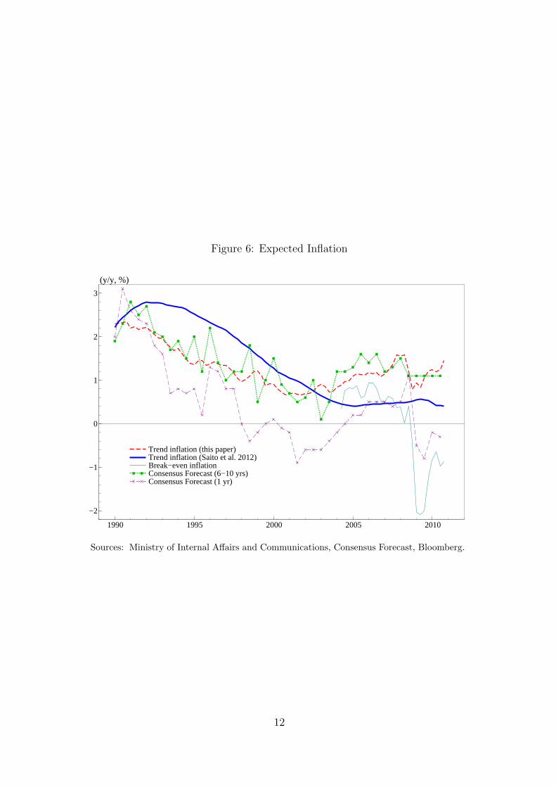
Figure 6: Expected Inflation
1990 1995 2000 2005 2010
−2
−1
0
1
2
3
(y/y, %)
Trend inflation (this paper) Trend inflation (Saito et al. 2012) Break−even inflation Consensus Forecast (6−10 yrs) Consensus Forecast (1 yr)
Sources: Ministry of Internal Affairs and Communications, Consensus Forecast, Bloomberg.
12

Figure 7: Granger Causality Tests
Long-runinflation
expectation
Short-runinflation
expectation
Actualinflation
1.09(0.30)
1.79(0.18)
3.69*(0.05)
0.66(0.42)
0.03 (0.86)
11.51** (0.00)-
����
������
@@
@@
@@
@@@I
�
��
��
��
���
@@@@
@@@@@R
Note: χ2 tests of linear restrictions on zero coefficients based on a tri-variate VAR model withconstant terms (sample period: 1990H1-2010H2). Figures in parentheses are q-values.Actual inflation is measured in terms of q/q of CPI (less food and energy). Long- andshort-run inflation expectations are “Trend inflation (this paper)” and “ConsensusForecast (1 yr)” in Figure 6.
have become negative since the Lehman shock (Figure 6). However, one should probablynot read too much into the negative break-even inflation rates due to the lack of marketliquidity in Treasury Inflation-Protected Securities (TIPS). The outstanding amount ofJapanese TIPS was mere USD84.5 billion at the end of March 2008, less than one fifth ofthe corresponding US value, and the Ministry of Finance has suspended the issuance ofinflation-indexed bonds since August 2008.
The other complication is related to short-run expected inflation, which occasionallytakes negative values since the 1990s. In their estimates of the Phillips curve, Fuhrer et al.(2011) argue that it is short-run expected inflation, rather than its long-run peer, that isrelevant for Japan’s inflation dynamics. However, the result does not accord with a simpleVAR estimation, which suggests that trend inflation causes actual inflation and short-runexpected inflation in a Granger sense, but not vice versa (Figure 7). Bernanke (2007) alsostresses the importance of long-run inflation expectations for price- and wage-setting.
3.1.2 Why have inflation expectations declined?
Turning to the question why expected inflation has declined over the past two decades orso, Saito et al. (2012) argue that, from a theoretical perspective, the reason is either thatthe central bank has lowered its target rate for inflation or that the public has becomemore suspicious about the achievability of the target rate once the nominal interest ratehas reached the zero floor.
13

The central bank’s communication strategy may also have mattered. Ito (a paneldiscussant) claims that the Bank of Japan’s (BoJ’s) projection for weak inflation mayhave had the effect of damping inflation expectations. Indeed, the BoJ, which began topublish its board members’ outlook for growth and inflation from 2000, often foresawweak price developments correctly. In contrast, the various long-run expected inflationrates mentioned above seem to have been more firmly anchored to positive values, afterthe BoJ announced its ‘understanding’ (now ‘goal’) of price stability in 2006.6 Table 4summarizes how the BoJ has communicated its thinking on price stability. This summaryreveals that (i) the BoJ has continuously defined price stability as a situation of neitherinflation nor deflation; (ii) the BoJ openly acknowledged as early as in 1997 the possibilityof a measurement bias, a year after the publication of the Boskin Report (Boskin et al.,1996); and (iii) the BoJ has improved its style of communication, for example, by puttinga numerical figure for the price stability goal.
As argued by Tobin (1972), Okun (1981) and Akerlof and Shiller (2009), public at-titudes (or ‘norm’) toward the price level may also have mattered in forming inflationexpectations. On that score, it is important to note that, in the 1990s, coupled with thevery strong yen, the public seems to have felt that prices in Japan were too expensivecompared to prices in other industrial countries. Or at least that is what the tone ofthe government and the media at the time, which tended to report that Japanese pricesshould be slashed, suggests (Table 5). In fact, that perception was warranted, as seenin the wide difference between domestic and foreign prices during the 1990s (Figure 17below). It was only after turn of the millennium that the media began to pay more atten-tion to the hazardous effects of deflation. The number of newspaper articles on deflationjumped in 2001, which may indicate that public attitudes toward the price level changeddiscontinuously at that time (Figure 8). The press coverage seems to have been affected bythe government’s “declaration of deflation” in 2001 and 2009, when its Monthly EconomicReport used the term “deflation,” as indicated in Table 5.
6As indicated by Table 4, the BoJ set a goal at 1 percent on February 14, 2012. Shirakawa (2012a)elaborates on its level by saying “[S]imply announcing out of the blue that the Bank aims to achieve 2percent inflation is not enough. Above all, this might raise unnecessary uncertainties for businesses andhouseholds. Furthermore, if the announcement was trusted and inflation expectations rose accordingly,it is financial markets that would respond most quickly. There would then be a risk of a premature risein long-term yields before actual prices and wages start to rise. Under such circumstances, the pricesof Japanese government securities, a large share of which is owned by financial institutions, would godown, thereby heightening the risk of undermining such institutions’ lending activities. Owing to theseconcerns, we judged that it was best to leave the CPI inflation rate at 1 percent for the time beingand exert efforts to achieve that goal. On top of this, the Bank will review “the price stability goal inthe medium to long term” once a year while analyzing the level of progress that has been made towardstrengthening the growth potential and the changes that have occurred in the general public’s perceptionof prices.”
14

Table 4: Bank of Japan’s Communication
1994-05-27: Principles for the Conduct and the Goal of Monetary Policy (Speech made by GovernorMieno) (authors’ translation)“One of main goals of monetary policy is delivering ‘sustainable growth without inflation’ in themedium- to long-run.” “The question is often posed on which price indicator, the Consumer PriceIndex or the Wholesale Price Index, the definition of price stability should be based. However, itis inappropriate to single out a price indicator, as the goal of monetary policy is the ‘stability ofprices’ not ‘stability of a price index.’”
1996-10-11: Financial Innovation, Financial Market Globalization, and Monetary Policy Management(Speech made by Governor Matsushita)“The Bank of Japan ... intends to manage monetary policy appropriately with the aim of main-taining price stability, preventing inflation or deflation of domestic prices.”
1997-06-27: A New Framework of Monetary Policy under the New Bank of Japan Law (Speech madeby Governor Matsushita)“It is, however, not easy to define price stability. There are diverse types of price indicators:for example, the Consumer Price Index, Wholesale Price Indexes, and the GDP deflator. Eachof these has its limitation, such as the range of items covered or the timing of release. Further,many studies have been conducted more recently on the possibility that these indicators offer asubstantially biased measurement of prices.”
2000-10-13: On Price Stability“[I]t is not deemed appropriate to define price stability by numerical values.” “Price stability,a situation neither inflationary nor deflationary, can be conceptually defined as an environmentwhere economic agents including households and firms can make decisions regarding such economicactivity as consumption and investment without being concerned about the fluctuation of thegeneral price level.”
2006-03-09: The Introduction of a New Framework for the Conduct of Monetary Policy“Price stability is a state where various economic agents including households and firms maymake decisions regarding such economic activities as consumption and investments without beingconcerned about the fluctuations in the general price level.” “Price stability is, conceptually, astate where the change in the price index without measurement bias is zero percent.”
2006-03-09: An Understanding of Medium- to Long-term Price Stability“It was agreed that, by making use of the rate of year-on-year change in the consumer price indexto describe the understanding, an approximate range between zero and two percent was generallyconsistent with the distribution of each Board member’s understanding of medium- to long-termprice stability. Most Board members’ median figures fell on both sides of one percent.”
2007-04-27: Outlook for Economic Activity and Prices“The ‘understanding’ expressed in terms of the year-on-year rate of change in the CPI, takes theform of a range approximately between 0 and 2 percent, with most Policy Board members’ medianfigures falling on one side or the other of 1 percent.”
2009-12-18 Clarification of the ‘Understanding of Medium- to Long-Term Price Stability’“In a positive range of 2 percent or lower, and the midpoints of most Policy Board members’‘understanding’ are around 1 percent.”
2012-02-14: The Price Stability Goal in the Medium to Long Term“The Bank judges that ‘the price stability goal in the medium to long term’ is in a positive rangeof 2 percent or lower in terms of the year-on-year rate of change in the consumer price index (CPI)and, more specifically, set a goal at 1 percent for the time being.”
15

Table 5: Government and Media Reports on Price Level
Government Reports1993 July: Annual Report on Japan’s Economy (FY1993)“While Japanese income per capita converted to US dollars is one of the highest in the world,living standards in reality as such are not. This is mainly because of the gap between internaland external prices. ... Consumers would be better off if prices in Japan declined, narrowing thisdomestic-foreign price difference.”
1999 June: Report of the Committee on Price Problems under Zero Inflation“Deflation is a situation where sub-par growth and a fall in prices take place simultaneously.” “Afall in prices does not necessarily incur recession.” “It would be appropriate for the authorities toaim at zero inflation. However, some margin needs to be taken into account, given the positivemeasurement bias in the consumer price index.”
2001 March: Monthly Economic Report“The Japanese economy is in a mild deflationary phase, if deflation is defined as ‘a continuingdecline in prices.’”
2001 December: Annual Report on Japan’s Economy and Public Finances (2000-2001)“[U]nder the current situation of the Japanese economy, even a mild deflation is believed to haveadverse effects on the economy.”
2009 November: Monthly Economic Report“Recent price developments show that the Japanese economy is in a mild deflationary phase.”
Op-Ed Articles in Major Newspapers1994-10-04: Can We Self-Praise Price Stability? (Nikkei Shimbun)“A 10% appreciation of the yen would increase households’ real purchasing power by 30 to 40thousands yens on average. The Price Report for FY1994, which the Economic Planning Agencypublished last week, stressed price stability amid the appreciation of the yen by presenting theabove estimation. The CPI increased by 1.2% in FY1993. ... However, the Report appears to singits own praises too much on price stability. In fact, consumer prices in Japan should have beenlowered.”
1998-07-27: Is Inflation Adjustment Really a Good Deal? (Asahi Shimbun)“Some commentators in the market as well as in academia have turned to inflation in order to liftthe economy. They claim that deliberately created inflation would sort out the problems of Japan’seconomy, where sales have declined and prices have fallen. This is so called ‘inflation adjustment.’... The costs of pursuing such a policy are much too large. It is difficult to imagine that this is aworthwhile policy.”
2001-03-17: Conquer Deflation, Once Admitted (Nikkei Shimbun)“Among major advanced economies, Japan is the only country where prices have continued todecline. The Government and the Bank of Japan should quickly come up with specific policies toconquer this deflation.”
2003-11-16: Don’t Forget the Homework of Conquering Deflation (Asahi Shimbun)“Deflation places a greater burden on firms and individuals who borrow money, as the amountthey have to pay back does not fall even when prices fall. This is the problem of deflation.”Note: Most of the quotes are the authors’ translation.
16

Figure 8: Press Coverage of Deflation
1990 1995 2000 2005 2010
2500
5000
7500
(No. of articles)
Note: The figure shows the number of hits for the search term “deflation” in articles ofmajor newspapers (Nikkei, Asahi, Mainichi, Yomiuri, Sankei). The figure for 2011 isthe annualized value of the number of hits for articles up to September that year.
3.2 The output gap
There is a consensus among researchers that the output gap has remained negative foralmost the entire period since the mid-1990s. Figure 9 shows various measures of theoutput gap. Both when employing a production function approach (BOJ) and a surveymeasure (Tankan), the results suggest that the output gap has remained negative sincethe early 1990s except for short intervals in the latter halves of the 1990s and the 2000s.The model-based measure by Saito et al. (2012) points to a broadly similar trend.
However, no consensus has emerged regarding why the output gap has remained neg-ative for such a long duration. As discussed below, there are various attempts to explainthe phenomenon. As these explanations are not mutually exclusive, it may well be thecase that the mechanisms they describe have worked simultaneously.
3.2.1 Why has the output gap remained negative for a long time?
The simplest answer to the question could be mere bad luck. Just “unfortunately,” Japanhas been hit by a series of large negative demand shocks. These include the demandshock resulting from the collapse of the asset price bubble in the early 1990s; the Japanesefinancial crisis and the Asian currency crisis in the latter half of the 1990s; the collapseof the US dotcom bubble in the early 2000s; and the global financial crisis in the latterhalf of the 2000s. Instead of sighing over these “unlucky” events, however, researchers aretrying to understand the forces underlying them. Since deterioration of the output gaphas been accompanied with a decline in the potential growth rate, researchers have beentrying to explain the link between two.
One strand of explanations of the negative output gap suggests that it is caused by a
17

Figure 9: Output Gaps
1985 1990 1995 2000 2005 2010−14
−12
−10
−8
−6
−4
−2
0
2
4
6
8
10
12
14(%)
BOJ Saito et al. (2012)
−40
−30
−20
−10
0
10
20
30
40
1985 1990 1995 2000 2005 2010
(%pt)
Tankan (rhs)
Note: “BOJ” refers to the output gap estimated by the Research and Statistics Department,Bank of Japan (Hara et al., 2006), while “Tankan” refers to the weighted averagesof the production capacity DI and employment conditions DI in the Tankan Corpo-rate Survey. The FY1990-2010 averages of capital and labor shares in the NationalAccounts are used as the weight. Finally, “Saito et al. (2012)” is the output gap esti-mated based on their DSGE model, where the output gap is defined as the deviationof real GDP from its potential level (Fueki et al., 2010). The shaded bars indicateperiods of recession.
18

Figure 10: Natural Rate of Interest
1980 1985 1990 1995 2000 2005 2010
−4
−3
−2
−1
0
1
2
3
4(%)
Japan United States
Note: Figures for the United States are originally from Williams (2009).
Source: Watanabe (2012).
decline in the natural rate of interest and the zero lower bound on the nominal interestrate. For instance, following the approach of Laubach and Williams (2003), Watanabe(2012) shows that, along with the potential growth rate, the natural interest rate in Japanhas declined to an extent that it has fallen into negative territory (Figure 10). In thatcase, once the central bank faced the zero floor, it was no longer able to lower the policyrate in tandem with the decline in the natural interest rate. This may have produced thenegative output gap, since the policy rate was too restrictive compared to the natural rate.Couching his argument in the Fisher equation, i = rn + πe, Watanabe (2012) suggeststhat instead of the negative inflation expectations πe, the reason why the economy hasfallen into a liquidity trap is the negative natural interest rate rn. Essentially, this line ofargument is same as Krugman’s (1998).
However, just like in the case of inflation expectations, whether the natural rate ofinterest, which is unobservable, has become negative is a matter of debate. Figure 11shows various measures of potential growth, which are assumed to be linked with thenatural rate of the interest rate. All of the measures of potential growth—be they basedon a production function approach (BOJ), estimates from a model (Saito et al., 2012), acorporate survey (Corporate) or the forecasts of economists (Consensus Forecast)—point
19

Figure 11: Potential Growth
1985 1990 1995 2000 2005 2010−2
0
2
4
(y/y, %)
BOJ Saito et al. (2012)
1985 1990 1995 2000 2005 2010−2
−1
0
1
2
3
4
5
Corporate (3 yrs) Consensus Forecast (6−10 yrs)
Note: “BOJ” refers to the potential growth rate estimated by the Research and StatisticsDepartment, Bank of Japan (Hara et al., 2006), while “Saito et al. (2012)” refers tothe potential growth rate estimated based on their DSGE model. “Corporate (3 yrs)”refers to the outlook for the 3 years ahead real demand growth rate for industry in theAnnual Survey of Corporate Behavior (Cabinet Office). Finally, “Consensus Forecast(6-10 yrs)” refers to the Consensus Forecast for the average real GDP growth rate forthe next 6 to 10 years.
to a decline in the potential growth rate, but none of them show a negative potentialgrowth rate except for a short interval around the Lehman crisis. Furthermore, in theiranalysis of historical decompositions of the inflation rate, Saito et al. (2012) show theeffects of the zero lower bound of the nominal interest rate on inflation are rather small,as long as these effects are captured by negative monetary policy shocks.7
Another strand of explanations sees a link between lower (but not necessarily nega-tive) potential growth and the deterioration in the output gap via growth expectations.Saito et al. (2012) argue that weaker growth expectations have squeezed demand morethan supply. The key question is whether permanent or transitory negative shocks onproductivity have lowered potential growth. In the case of permanent shocks, a “pre-
7As seen in footnote 5, the DSGE model of Saito et al. (2012) does not explicitly model the zero lowerbound and thus estimated monetary policy shocks are assumed to capture the effects of the zero lowerbound.
20

emptive” reaction of the demand side to a future decline in supply potential may reducedemand heavily and thus lead to deterioration in the output gap. On the other hand, inthe case of transitory shocks, consumption smoothing may lead to a limited reaction onthe demand side and thus improve the output gap. Saito et al. (2012) show, in line withthis kind of reasoning, a permanent negative shock to productivity drags down inflation,while a transitory shock lifts inflation (Figure 12).8
Moreover, they also explore the theoretical possibility that prices become weaker if,for some reasons (lack of innovative entrepreneurs, government regulation, etc.), the sup-ply side of the economy cannot fully respond to a change in the demand structure. Forinstance, it is widely assumed that population aging leads to changes in the demand struc-ture, such as greater demand for health care and less demand for, say, automobiles. If thequantity and price of health care services are heavily regulated and cannot accommodatethe growing demand of the elderly, then general prices may decline, as the elderly maysave their money instead of purchasing automobiles in the expectation that health careservices will be provided in the future. Another study that examines the impacts of pop-ulation aging on inflation through changes in the demand structure is that by Katagiri(2012) who uses a multi-sector DSGE model with search friction. Meanwhile, Kimuraet al. (2010), while not treating the output gap explicitly, argue that a decline in the nat-ural rate of interest may reduce private expenditure, because an increase in the presentdiscount value of government debt may reduce private expenditure.
Yet another strand of explanations focuses on the financial side. Given that Japan’sgrowing government debt has been financed by banks which have increased their purchasesof Japanese Government Bonds (JGBs) (Figure 13), the question naturally arises whetherthere is any relationship between the behavior of banks and the output gap. Aoki andSudo (2012) construct another DSGE model, in which the Value-at-Risk (VaR) constraintleads banks to accumulate large amount of JGBs instead of financing private investment(a crowding-out-like phenomenon).9 They show that this worsens the output gap and thusputs downward pressures on prices (upper panels of Figure 14). They also demonstrate
8Just like the FRB/EDO model, Saito et al. (2012) construct a two-sector model, in which bothpermanent and transitory shocks are embedded in production functions of both sectors such as:
Xct = [Ku,c
t ]α[(Am
t Zmt )Lc
t ]1−α
,
Xkt =
[Ku,k
t
]α [(Am
t Zmt )(Ak
tZkt )L
kt
]1−α,
where Xt is output, Kut is the effective capital input, and Lt is the labor input in consumption-goods-
producing sector c and investment-goods-producing sector k. Ant and Zn
t are technology shocks, with theformer stationary in levels and the latter stationary in growth rates:
lnAnt = lnAn
∗ + εa,nt , n ∈ m, k
lnZnt − lnZn
t−1 = (1− ρz,n) ln Γn∗ + ρz,n(lnZn
t−1 − lnZnt−2) + εz,nt ,
where superscript m indicates economy-wide and k the investment-goods-producing sector. An∗ and Γn
∗are the constant technology level and the constant growth rate, respectively. εa,nt and εz,nt correspond totransitory and permanent shocks. See Fueki et al. (2010) for more details.
9Following Adrian and Shin (2010), they model the VaR constraint as the non-negative return on
21

Figure 12: Effects of Temporary and Permanent Productivity Shocks
0 5 10 15 20
−0.02
0.00
0.02
Response of real GDP to a temporary productivity shock (%pt)
(quarters)
0 5 10 15 20
0.00
0.01
0.02
Response of infaltion to a temporary productivity shock (%pt)
(quarters)
0 5 10 15 20
−2.0
−1.5
−1.0
−0.5
0.0Response of real GDP to a permanent productivity shock (%pt)
(quarters)
0 5 10 15 20
−0.10
−0.05
0.00
Response of inflation to a permanent productivity shock (%pt)
(quarters)
Note: Reactions to a negative one standard error shock to economy-wide productivity. Thedotted lines show the 90% confidence interval.
Source: Saito et al. (2012).
22

Figure 13: Banks’ Portfolio
1980 1990 2000 2010
10
15
20(Share, %)
Government Bonds
1980 1990 2000 2010
55
60
65
70
(Share, %)
Loans
Source: Aoki and Sudo (2012).
that a decline in the potential growth rate due to a negative permanent productivity shocktightens the VaR constraint and thus puts downward pressure on inflation (lower panelsof Figure 14).10
3.3 Related issues
If, as suggested above, the lower natural rate of interest or lower potential growth isresponsible for the prolonged negative output gap, the next question that arises is whyJapan’s growth potential has declined. Including Hayashi and Prescott’s (2002) seminalstudy of Japan’s ‘lost decade,’ there is an extensive literature on this issue, which it isbeyond the scope of this paper to examine. At the conference, like Shirakawa (2012b),Watanabe (2012) and Ueda (concluding remarks) suggest that the malfunction of financialintermediaries after the collapse of the asset price bubble as well as the demographic trendsof population aging and decline (Figure 15) may have played a role. Recently, Nishimura
bank’s net portfolio at the time of the worst outcome:
rk,t+1kt(i) + rb,t+1bt(i)− rd,tdt(i) ≥ 0,
where kt(i), bt(i) and dt(i) are capital stock (which banks own through their loans), government bonds anddeposits on bank i’s balance sheet. rk,t+1 and rb,t+1 are the worst return on kt(i) and bt(i) respectively,which are assumed to follow certain stochastic processes. rd,t is the predetermined interest rate on bankdeposits. The constraint results in the spread
rk − rb =1− γrdγrd
(rb − rk),
where γ is the survival probability of the bank. The impulse responses to a shock to bank capital can beexpressed by a decline in γ.
10The impulse responses of inflation in Figure 14 dissipate more quickly than those in Figure 12. Thismay be primarily because Aoki and Sudo (2012) did not incorporate inflation indexation in their model.
23

Figure 14: Effects of the VaR Constraint
0 5 10 15 20
−0.06
−0.04
−0.02
0.00Response to a shock to banks’ net worth (%pt)
(quarters)
Output
0 5 10 15 20
−0.03
−0.02
−0.01
0.00
0.01Response to a shock to banks’ net worth (%pt)
(quarters)
Inflation
0 5 10 15 20
−0.05
−0.04
−0.03
−0.02
−0.01
0.00Response to a permanent productivity shock (%pt)
(quarters)
Output (with VaR) Output (w/o VaR)
0 5 10 15 20
−0.04
−0.02
0.00 Response to a permanent productivity shock (%pt)
(quarters)
Inflation (with VaR) Inflation (w/o VaR)
Note: Reactions to a negative one standard error shock to banks’ net worth and permanentproductivity.
Source: Aoki and Sudo (2012).
24

Figure 15: Asset Prices and Demography
1960 1970 1980 1990 2000 2010 2020
60
70
80
90
Working−age population
(Million)
Working−age population Forecast
1980 1985 1990 1995 2000 2005 2010
50
100
150
200(Index, CY2000=100)
Land pricesCommercial property Residential property
Sources: Japan Real Estate Institute, Ministry of Health, Labour and Welfare.
(2011) has highlighted the link between these two factors using an overlapping generationsmodel in which demographic aging and decline trigger a drop in asset prices and thus leadto a distortion in financial intermediation. On the other hand, Ikeda and Saito (2012)have constructed a DSGE model in which a decline in the working-age population lowersthe real interest rate and that effect is amplified by a fall in land prices in the presenceof collateral constraints.
Another separate issue is why the slope of the Phillips curve has become flatter, asseen in Figure 5. Again, an extensive literature has developed in the context of the GreatModeration. Potential explanations of the flattering of the Phillips curve in Japan thathave been advanced include, among others, that the impact of the global output gap onJapan’s inflation has increased as a result of globalization (Borio and Filardo, 2007), orthe strategic complementarity in firms’ price-setting behavior plays a role (Watanabe,2012).
25

Figure 16: Exchange Rates and Import Prices
1985 1990 1995 2000 2005 2010
50
75
100
125
150
(Index CY2005=100)
NEER REER
−25
0
25
−2.5
0.0
2.5
1985 1990 1995 2000 2005 2010
(y/y, %) (y/y, %)
Import price index (in yen) CPI less fresh food (rhs)
Sources: Bank for International Settlements, Bank of Japan, Ministry of Internal Affairs andCommunications.
3.4 Other Factors
In an open economy setting, external factors are added to a Phillips curve such as the onerepresented by equation (1). For instance, since Japan heavily relies on imports of naturalresources, commodity prices are frequently added to the equation. However, given thedevelopments in the energy components shown in Table 1, developments in commodityprices, including energy, cannot explain the chronic deflation in Japan. Import prices,which largely reflect developments in commodity prices, have shown a number of ups anddowns, which is in contrast with the prolonged and steady decline in consumer prices(lower panel of Figure 16). For this reason, below, we will focus on other external factors,namely the exchange rate and domestic-foreign price differences.
3.4.1 Does the appreciation of the yen matter?
Over the past few decades, the yen’s nominal effective exchange rate (NEER) has ap-preciated as a trend (upper panel of Figure 16). At the same time, although evidence isstill mixed, the pass-through of changes in the exchange rate may have declined, as, for
26

example Otani et al. (2003) suggest. If this is indeed the case, then, at least superficially,it might seem rather difficult to argue that the appreciation of the yen has played a sig-nificant role in deflation in Japan. However, Fukuda (a panel discussant) suggests thatif the equilibrium mark-up diminished along with the declining pass-through, this wouldlead to lower prices domestically.
There are other arguments that suggest that the appreciation of the yen matters.For instance, Watanabe (2012) demonstrates theoretically that, as argued by McKinnonand Ohno (2001), once expectations of yen appreciation are firmly embedded among thepublic, Japan may fall into a liquidity trap in the presence of the zero lower bound on thenominal interest rate. Heuristically, if uncovered interest rate parity holds, i.e., i = i∗+∆d,where i∗ is the short-term nominal interest rate in a foreign country and ∆d is the expectedrate of depreciation, i may be subject to the zero lower bound and the economy may hencefall into a liquidity trap, when ∆d < 0 (i.e., when the yen appreciates). Furthermore, aswill be discussed below, Iwasaki et al. (2012) show that the less flexible exchange rateregime of the Chinese renminbi has the effect of amplifying downward pressure of Chineseproductivity shocks on Japanese inflation.
3.4.2 Do domestic-foreign price differences matter?
As seen in Table 5, in the 1990s, wide differences between domestic and foreign prices werea matter of concern for both policy makers and the public. The 1990s were indeed a periodin which prices in Japan were considerably higher than those in other major advancedeconomies (upper panels of Figure 17). However, the difference declined substantiallyin the 2000s. Similar observations can be made with regard to GDP per capita (lowerpanels of Figure 17).11 As highlighted by Maeda (a panel discussant), Japan deregulatedin a wide range of areas during the late 1990s and early 2000s including zoning laws forlarge retailers, which may have contributed to slashing domestic-foreign price differencesby reducing margins and/or improving productivity in the distribution chain.12
Supply shocks in emerging economies may also matter. Although supply shocks, asSekine (2009) suggests, have affected inflation not only in Japan but also in other indus-trial economies, the impact may have been more pronounced in Japan as a result of theclose trade links with the dynamic emerging economies of Asia, particularly China. Usingindustrial panel data, Iwasaki et al. (2012), for instance, find that the impact of a highershare of imports from emerging economies, which can be regarded as a proxy of produc-tivity shocks in these economies, is greater in Japan than in the United States and Europe(Table 6). Furthermore, they construct a three-sector, three-country DSGE model (con-sisting of a tradable final goods, a tradable intermediate goods, and a non-tradable goods
11The positive correlation between price levels and real GDP per capita is often taken as evidence ofthe Balassa-Samuelson effect.
12An effect of narrower margins can be captured by a markup shock in the New Keynesian PhillipsCurve estimated by Saito et al. (2012). It might be possible to obtain more direct evidence for a changein margins using firm-level data, as demonstrated by Ariga et al. (1999). Unfortunately, there are nostudies that have pursued this avenue of research in recent years.
27

Figure 17: Deviation from Purchasing Power Parity (PPP)
1980 1990 2000 2010
1.0
1.5
(Domestic prices/US prices)
(Domestic prices/US prices × 100)
United Kingdom Japan Euro area
1980 1990 2000 2010
1
2
3
4(Domestic prices/Weighted average of trade partners’ prices)
United Kingdom Japan United States Euro area
0 2 4 60
20
40
60
80
100
120
140
160
180Japan (as of 1995)
(Real GDP per capita, USD 10,000)
0 2 4 60
20
40
60
80
100
120
140
160
180
Japan
(as of 2009)
(Real GDP per capita, USD 10,000)
(Domestic prices/US prices × 100)
Note: Figures in upper panels are domestic-foreign price differences calculated as P/P ∗e,where P is domestic prices, P ∗ is foreign prices and e is the market exchange rates.In the left-hand side, P ∗ is US prices and e is the bilateral exchange rates againstthe US dollar, whereas in the right-hand side P ∗ is prices of major trade partnersand e is the nominal effective exchange rates. In the left-hand side, P/P ∗ is obtainedfrom the PPP exchange rate in the IMF World Economic Outlook database and efrom Bloomberg. In the right-hand side, e is obtained from the BIS nominal effectiveexchange rates (narrow base comprising 27 economies) and P/P ∗ are calculated bythe authors using the above bilateral PPP exchange rate and the weights of the BISNEERs. Lower panels are scatter diagrams of OECD countries (less Luxembourg).Real GDP per capita is based on the PPP exchange rates.
Sources: Bank for International Settlements, International Monetary Fund, Bloomberg, PennWorld Table 7.0.
28

sector with the countries corresponding to Japan, China, and the United States) whichincorporates the features that (i) Japan heavily exports intermediate goods to China inexchange for final goods; (ii) Japan-China trade links are stronger than Japan-US andUS-China trade links; (iii) intermediate goods are less substitutable than final goods; and(iv) the Chinese renmenbi is fixed to the US dollar.13 Their impulse response analysis of arise in Chinese productivity in the tradable final goods sector shows that Japanese infla-tion falls more than US inflation (Figure 18). This is because, given the strong trade links,Japan imports more low-cost final goods from China than the United States. Despite anincrease in imports from China, Japan’s trade balance is less deteriorated than that ofthe United States, since more final goods production in China leads to higher demandfor Japanese intermediate goods. The model suggests that this results in an appreciationof the yen vis-a-vis the US dollar, which puts additional downward pressure on Japaneseinflation. This deflationary impact could be mitigated if China were to adopt a moreflexible exchange rate regime.
4 Conclusion
In November 2011, the Bank of Japan, together with the University of Tokyo, held aone-day conference to take stock of researches on the chronic deflation which has gripped
13The trade structure in the model is largely determined by aggregate intermediate goods T1,t(hJ2 ) and
final goods T2,t(jJ) for a final goods producer hJ
2 , and a household jJ (superscript J stands for Japan),where aggregation takes place such that:
T1,t(hJ2 ) =
[(µJ
J)1
ϕJ1 QJ
1,t(hJ2 )
1− 1
ϕJ1 + (µJ
U )1
ϕJ1 MU
1,t(hJ2 )
1− 1
ϕJ1 + (µJ
C)1
ϕJ1 MC
1,t(hJ2 )
1− 1
ϕJ1
] ϕJ1
ϕJ1−1
,
T2,t(jJ ) =
[(νJJ )
1
ϕJ2 QJ
2,t(jJ)
1− 1
ϕJ2 + (νJU )
1
ϕJ2 MU
2,t(jJ)
1− 1
ϕJ2 + (νJC)
1
ϕJ2 MC
2,t(jJ)
1− 1
ϕJ2
] ϕJ2
ϕJ2−1
.
Here, QJ1,t(h
J2 ) and QJ
2,t(jJ ) are intermediate goods and final goods made by domestic producers, and
M i1,t(h
J2 ) and M i
2,t(jJ ) are those imported from the United States (i = U) and China (i = C). Similar
equations are defined for the United States and China. Iwasaki et al. (2012) set the elasticities ofsubstitution such that ϕi
1 < ϕi2 (i ∈ J, U,C) to express (iii). Furthermore, they adjust shares µJ
i and νJito capture (i) and (ii). More specifically, they assume the following trade balances in a steady-state andadjust parameters to replicate them.
US China
Japan
1.5 7.0
1.5 7.0
1.0
1.0 -���
���
@@
@@@I@
@@@@R
�
��
���
The figures are in terms of percent of GDP. They are provided here for an illustrative purposes only anddo not exactly match those in their model. Thin lines represent trade flows in intermediate goods, whilethick lines represent those in final goods.
29

Table 6: Impact of Import Competition from Emerging Market Economies
Japan US EuropeImport share -4.689* -2.352** -3.531**
(2.524) (0.515) (0.964)Sample periods 1989-2007 1997-2006 1995-2008Number of observations 988 2,702 7,010Number of sectors 52 325 618
Note: Figures in parentheses are standard errors. * and ** denote significanceat the 5% and 1% confidence levels, respectively. Dependent variablesare inflation measured by the producer price index (domestic corporategoods price index in the case of Japan). Industrial panel regressions usingthe growth rates of manufacturing outputs in the EMEs multiplied bya sector’s (average) labor intensity as instrument variables. Fixed andtime effects are controlled for. Results of the United States and Europeare from Auer and Fischer (2010) and Auer et al. (2010).
Sources: Iwasaki et al. (2012), Auer and Fischer (2010), Auer et al. (2010).
Figure 18: Supply Shocks from China
0 5 10 15 20
−0.01
0.00
0.01
0.02
0.03Responses of inflation (%pt)
(quarters)
Japan United States China
0 5 10 15 20
−0.2
−0.1
0.0
0.1
0.2
0.3
Responses of trade balance (%pt)
(quarters)
Note: Reactions to a positive productivity shock in China’s tradable final goods sector.
Source: Iwasaki et al. (2012).
30

Japan since the latter half of the 1990s. The present paper represents an attempt tosynthesizes the studies presented at the conference by considering the various hypothesesput forward to explain this period of prolonged deflation. Specifically, causes that havebeen proposed include the zero-lower bound on the nominal interest rate; public attitudes(‘norm’) toward the price level; central bank communication; weaker growth expecta-tions coupled with declining potential growth or the lower natural rate of interest; riskaverse banking behaviors; deregulation in the distribution chain; and the rise of emergingeconomies.
In fact, some of these potential causes were already alluded to at the time of workshopsheld by the Bank of Japan in 2001. For instance, the idea that Japan had fallen into aliquidity trap was widely discussed in the literature at the time. This does not mean,however, that the conference in 2011 had little new to add. On the contrary, the studiesthat were presented provided important new insights that benefited from the accumulationof data over the past decade as well as advances in economics. The fact that Japan didnot experience a severe acceleration of deflation (i.e., deflationary spiral) despite the largenegative output gap seems to support the hypothesis that Japan has been stuck at adeflationary equilibrium due to a liquidity trap, the reason for which—such as negativeinflation expectations, a negative natural interest rate, or expectations of the appreciationof the yen—however, are not fully understood. At the same time, the accumulated dataover the years suggest that the fiscal multiplier does not appear to have increased as theorywould lead one to expect. This has led researchers to look for alternative explanationsas demonstrated by the papers submitted to the conference. Similarly, researchers atthe conference benefited from advances in DSGE modeling techniques, which lead to abetter understanding of inflation expectations, of the link between the output gap andthe potential growth rate (the decline in which had become clearer during the decade),and of issues related with globalization.
The conference leaves a long list of hypotheses. At this stage of investigation, it is stilldifficult to single out one specific or dominant explanation for Japan’s prolonged periodof deflation and it may well be the case that it is the result of a combination of factors.We hope that further researches will shed more light on the issue. At the same time, ashighlighted by Miyao et al. (2008), it may be necessary to revisit another issue associatedwith chronic deflation, namely its costs, which were not fully addressed by this conference.In any case, a better understanding of the causes of chronic deflation is important not onlyfor curing Japan’s ailing economy, but also for preventing other countries from sufferinga similar fate.
31

Appendix 1: Estimation of the Phillips Curve and
Trend Inflation
This appendix presents details of the procedures for estimating the Phillips curve withtime-varying parameters and trend inflation. It also touches upon the historical decom-position of inflation dynamics.
Time-Varying Parameter Phillips Curve
The New Keynesian model as the standard framework for monetary policy analysis typ-ically specifies inflation dynamics using the following equation, which is called a hybridNew Keynesian Phillips curve (NKPC):
πt = ρπt−1 + ζGapt + bEtπt+1 + ut, (3)
where πt is the rate of inflation in period t; Gapt is the output gap, which is used as aproxy variable for marginal costs; Etπt+1 is one-period ahead expected inflation, where Et
is an expectation operator; and ut represents shocks or other factors that are not capturedby the explanatory variables. These are assumed to include effects from changes in importcosts and mark-ups, etc.
Equation (3) assumes that trend inflation is zero or some constant value. Cogley andSbordone (2008) relax this assumption and derive the following equation.14
(πt − πt) = ρt(πt−1 − πt) + ζtGapt + b1tEt(πt+1 − πt)
+ b2tEt
∞∑j=2
φj−11t (πt+j − πt) + ut, (4)
Equation (4) differs from (3) in two respects: first, equation (4) includes additional ex-planatory variables such as trend inflation πt and higher-order inflation expectationsEt
∑∞j=2 φ
j−11t (πt+j − πt); second, as indicated by the subscripts on the parameters on
lagged inflation and the output gap, the parameters are not invariant over time. In fact,Cogley and Sbordone (2008) show that there is a relationship between each parameterand trend inflation such that higher trend inflation implies a lower weight on the currentoutput gap and a greater weight on expected future inflation.
Estimating the time-varying Phillips curve
Estimation of a time-varying parameter NKPC involves two steps. In the first step, areduced-form VAR is estimated. In the next step, the parameters of the NKPC are
14The original equation derived by Cogley and Sbordone (2008) includes additional terms such as theexpectations of the discount factor and real output growth. We omit these terms because preliminary esti-mation indicates that their contributions are negligible. In fact, Cogley and Sbordone (2008) themselves,using U.S. data, find that excluding these terms has little impact on the estimation results.
32

obtained by matching the conditional expectations generated from the VAR and theNKPC.
Step 1: Estimating the reduced-form VAR
To begin with, a reduced-form VAR with time-varying parameters and stochasticvolatility is estimated using the following specification:15
xt = X′
tΘt + ϵxt,
where xt is a vector of endogenous variables X′t = I ⊗ [1 x
′t−l]; xt−l represents lagged
values of xt, where the maximum lag is set to two; and Θt is a vector of time-varyingparameters.
Endogenous variables are the inflation rate πt measured in terms of CPI less fresh foodand adjusted to exclude the effects of changes in the consumption tax rate and subsidiesfor high school tuition, and the output gap Gapt estimated by the Research and StatisticsDepartment, Bank of Japan.16 The data sample covers the period 1980Q1-2010Q4 andthe data up to 1985Q4 are used as a training sample for initializing the prior. In orderto estimate trend inflation effectively, we extend Cogley and Sbordone’s approach byincluding inflation expectations from the survey (expected rate of inflation for six to tenyears ahead, published in the Consensus Forecasts).17
Time-varying parameter Θt and VAR innovations ϵxt follow a random walk processand a geometric random walk process respectively,
Θt = Θt−1 + vt,
ϵxt = V1/2t ξt,
Vt = B−1HtB−1,
lnhit = lnhit−1 + σiηit.
where Ht is a diagonal matrix with elements hit, B is a lower triangular matrix, and vt, ξt,and ηt follow a standard normal distribution. B and σi are estimated.
15The estimation is based on an MCMC algorithm using the hyper-parameter of Cogley and Sbordone(2008).
16As a proxy variable for marginal costs, Cogley and Sbordone (2008) use the labor share of nationalincome instead of the output gap.
17To be more precise, we add an observation equation with a measurement error term to the abovereduced-form VAR.
33

Step 2: Matching the expectation formation processes
Next, we will match the expectation formation process of the reduce-form VAR withthat of the NKPC. The reduced-form VAR can be rewritten as
zt = µt + Atzt−1 + ϵzt, (5)
where zt = (xt, xt−1, · · · , xt−p+1)′. Then, the conditional expectations of inflation mea-
sured by the deviations from trend inflation can be expressed as
E(πt|zt−1) = e′
πAtzt−1,
where ek is a selection vector picking up variable k, and zt = zt − (I − At)−1µt. The
conditional expectation of inflation derived from the time-varying parameter NKPC is
E(πt|zt−1) = ρe′
πzt−1 + ξe′
GapAtzt−1 + b1e′
πA2t zt−1 + b2e
′
π(I − φ1At)−1A3
t zt−1.
This implies
e′
πAt = ρe′
πI + ξe′
GapAt + b1e′
πA2t + b2e
′
π(I − φ1At)−1A3
t ≡ g(µt, At, ψ),
where ψ represents the parameters of the Calvo model (α, ρ, θ), where α is the fractionof sticky-price firms, ρ is the degree of indexation, and θ is the elasticity of substitutionamong differentiated goods. We obtain these parameter values by minimizing the squareof e
′πAt − g(µt, At, ψ) given µt and At of the reduced-form VAR (5).
Historical Decomposition of Inflation Dynamics
The historical decomposition of inflation in Table 3 is conducted by using the followingequation, which is obtained by solving equation (4) forward:18
πt = (1− ρt)πt + ρtπt−1 + Et
∞∑j=0
φj1tζtGapt+j + ut.
18Since estimates of b2t are de-minimis, Et
∑∞j=2 φ
j−11t (πt − pit) is ignored here.
34

Appendix 2: Conference Program
Price Developments in Japan and Their Backgrounds:Experiences Since the 1990s
4th Joint Conference by the Center for Advanced Research in Finance of the
University of Tokyo and the Research and Statistics Department of the Bank of Japan
(November 24, 2011, Bank of Japan)
9:00 Opening Remarks Eiji Maeda, Bank of Japan
9:05 Opening SessionBackgrounds of Price Developments in Japan: Facts and IssuesPresenter Kenji Nishizaki, Bank of Japan
9:50 Session 1Chairperson Ryuzo Miyao, Bank of Japan
Long-Lasting Deflation under the Zero Interest Rate EnvironmentPresenter Tsutomu Watanabe, Tokyo UniversityDiscussant Kenn Ariga, Kyoto University
Structural Problems and Price Dynamics in JapanPresenters Ichiro Fukunaga, Bank of Japan
Masashi Saito, Bank of JapanDiscussant Yasushi Iwamoto, Tokyo University
12:00 Lunch
13:30 Session 2Chairperson Yuzo Honda, Kansai University
Impacts of Supply Shocks from Emerging EconomiesPresenters Masahiro Kawai, Asian Development Bank
Naohisa Hirakata, Bank of JapanDiscussant Yoichi Matsubayashi, Kobe University
Asset Portfolio Choice of Banks and Inflation DynamicsPresenters Kosuke Aoki, Tokyo University
Nao Sudo, Bank of JapanDiscussant Yosuke Takeda, Sophia University
15:30 Coffee Break
35

15:45 Panel DiscussionModerator Kiyohiko G. Nishimura, Bank of JapanPanelists Takatoshi Ito, Tokyo University
Toshiki Jinushi, Kobe UniversityShin-ichi Fukuda, Tokyo UniversityEiji Maeda, Bank of Japan
17:45 Concluding RemarksKazuo Ueda, Tokyo University
18:00 Adjournment
36

References
Adrian, T. and H. S. Shin (2010): “Financial Intermediaries and Monetary Eco-nomics,” in Handbook of Monetary Economics, 1st edition, ed. by B. M. Friedman andM. Woodford, Elsevier, vol. 3, chap. 12, 601–650.
Akerlof, G. A. and R. J. Shiller (2009): Animal Spirits: How Human PsycologyDrives the Economy, and Why It Matters for Global Capitalism, Princeton UniversityPress.
Aoki, K. and N. Sudo (2012): “Asset Portfolio Choice of Banks and Inflation Dy-namics,” Paper presented at the conference on Price Developments in Japan and TheirBackgrounds: Experiences Since the 1990s, November 24, 2011, Bank of Japan, forth-coming in English as a Bank of Japan Working Paper (No. 12-J-4 in Japanese).
Ariga, K., Y. Ohkusa, and K. G. Nishimura (1999): “Determinants of Individual-Firm Markup in Japan: Market Concentration, Market Share, and FTC Regulations,”Journal of the Japanese and International Economies, 13, 424–450.
Auer, R. and A. M. Fischer (2010): “The Effect of Low-Wage Import Competitionon U.S. Inflationary Pressure,” Journal of Monetary Economics, 57, 491–503.
Auer, R. A., K. Degen, and A. M. Fischer (2010): “Globalization and Inflation inEurope,” CEPR Discussion Papers 8130, Centre for Economic Policy Research.
Benhabib, J., S. Schmitt-Grohe, and M. Uribe (2001): “The Perils of TaylorRules,” Journal of Economic Theory, 96, 40 – 69.
Bernanke, B. S. (2007): “Inflation Expectations and Inflation Forecasting,” Speechat the Monetary Economics Workshop of the National Bureau of Economic ResearchSummer Institute.
Borio, C. and A. Filardo (2007): “Globalisation and Inflation: New Cross-CountryEvidence on the Global Determinants of Domestic Inflation,” BIS Working Papers 227,Bank for International Settlements.
Boskin, M. J., E. R. Dulberger, R. J. Gordon, Z. Griliches, and D. Jor-genson (1996): “Toward a More Accurate Measure of the Cost of Living: The FinalReport of the Advisory Commission to Study the Consumer Price Index,” Social Secu-rity Online, History Home.
Bullard, J. (2010): “Seven Faces of “The Peril”,” Federal Reserve Bank of St. LouisReview of Economic Dynamics, 92, 339–352.
Chung, H. T., M. T. Kiley, and J.-P. Laforte (2010): “Documentation of theEstimated, Dynamic, Optimization-Based (EDO) Model of the U.S. Economy: 2010Version,” Finance and Economics Discussion Series 2010-29, Board of Governors ofthe Federal Reserve System.
37

Cogley, T. and A. M. Sbordone (2008): “Trend Inflation, Indexation, and InflationPersistence in the New Keynesian Phillips Curve,” American Economic Review, 98,2101–2126.
Edge, R. M., M. T. Kiley, and J.-P. Laforte (2007): “Documentation of theResearch and Statistics Division’s Estimated DSGE Model of the U.S. Economy: 2006Version,” Finance and Economics Discussion Series 2007-53, Board of Governors ofthe Federal Reserve System.
Fueki, T., I. Fukunaga, H. Ichiue, and T. Shirota (2010): “Measuring PotentialGrowth with an Estimated DSGE Model of Japan’s Economy,” Bank of Japan WorkingPaper Series, No. 10-E-13, Bank of Japan.
Fuhrer, J. C., G. P. Olivei, and G. M. B. Tootell (2011): “Inflation DynamicsWhen Inflation is Near Zero,” Working Papers 11-17, Federal Reserve Bank of Boston.
Hara, N., N. Hirakata, Y. Inomata, S. Ito, T. Kawamoto, T. Kurozumi,M. Minegishi, and I. Takagawa (2006): “The New Estimates of Output Gap andPotential Growth Rate,” Bank of Japan Review Series, 2006-E-3.
Hayashi, F. and E. C. Prescott (2002): “The 1990s in Japan: A Lost Decade,”Review of Economic Dynamics, 5, 206–235.
Ikeda, D. and M. Saito (2012): “The Effects of Demographic Changes on the RealInterest Rate in Japan,” Bank of Japan Working Paper Series, No. 12-E-3, Bank ofJapan.
Iwasaki, Y., M. Kawai, and N. Hirakata (2012): “Monetary Policy, ExchangeRate Regimes and Three-Way Trade,” Paper presented at the conference on PriceDevelopments in Japan and Their Backgrounds: Experiences Since the 1990s, November24, 2011, Bank of Japan, forthcoming in English as a Bank of Japan Working Paper(No. 12-J-7 in Japanese).
Katagiri, M. (2012): “Economic Consequences of Population Aging in Japan: Effectsthrough Changes in Demand Structure,” IMES Discussion Paper Series 12-E-03, In-stitute for Monetary and Economic Studies, Bank of Japan.
Kimura, T., T. Shimatani, K. Sakura, and T. Nishida (2010): “The Role ofMoney and Growth Expectations in Price Determination Mechanism,” Bank of JapanWorking Paper Series, 2010-E-11, Bank of Japan.
Krugman, P. R. (1998): “It’s Baaack: Japan’s Slump and the Return of the LiquidityTrap,” Brookings Papers on Economic Activity, 137–205.
Laubach, T. and J. C. Williams (2003): “Measuring the Natural Rate of Interest,”Review of Economics and Statistics, 85, 1063–1070.
38

McKinnon, R. and K. Ohno (2001): “The Foreign Exchange Origins of Japan’s Eco-nomic Slump and Low Interest Liquidity Trap,” World Economy, 24, 279–315.
Miyao, R., K. Nakamura, and T. Shirota (2008): “Costs of Price Fluctuations:Literature Survey and Empirical Assessment,” Bank of Japan Working Paper Series,No. 2008-J-2, Bank of Japan, in Japanese.
Nishimura, K. G. (2011): “Population Ageing, Macroeconomic Crisis and Policy Chal-lenges,” Speech at the 75th Anniversary Conference of Keynes’ General Theory, Uni-versity of Cambridge.
Okun, A. M. (1981): Prices and Quantities: A Macroeconomic Analysis, Basil Blackwell.
Otani, A., S. Shiratsuka, and T. Shirota (2003): “The Decline in the ExchangeRate Pass-Through: Evidence from Japanese Import Prices,” Monetary and EconomicStudies, 21, 53–81.
Saito, M., T. Fueki, I. Fukunaga, and S. Yoneyama (2012): “Structural Problemsand Price Dynamics in Japan,” Paper presented at the conference on Price Develop-ments in Japan and Their Backgrounds: Experiences Since the 1990s, November 24,2011, Bank of Japan Working Paper Series, No. 12-J-2, Bank of Japan, in Japanese.
Sekine, T. (2009): “Another Look at Global Disinflation,” Journal of the Japanese andInternational Economies, 23, 220–239.
Shirakawa, M. (2012a): “Japan’s Economy and Monetary Policy” Speech at a MeetingHeld by the Naigai Josei Chousa Kai (Research Institute of Japan) in Tokyo.
Shirakawa, M. (2012b): “Deleveraging and Growth: Is the Developed World FollowingJapan’s Long and Winding Road?” Lecture at the London School of Economics andPolitical Science (Co-hosted by the Asia Research Centre and STICERD, LSE).
Sudo, N. (2011): “Accounting for the Decline in the Velocity of Money in the JapaneseEconomy,” IMES Discussion Paper Series 11-E-16, Institute for Monetary and Eco-nomic Studies, Bank of Japan.
Tobin, J. (1972): “Inflation and Unemployment,” American Economic Review, 62, 1–18.
Watanabe, T. (2012): “Long-Lasting Deflation under the Zero Interest Rate Environ-ment,” Paper presented at the conference on Price Developments in Japan and TheirBackgrounds: Experiences Since the 1990s, November 24, 2011, Bank of Japan WorkingPaper Series, No. 12-J-3, Bank of Japan, in Japanese.
Williams, J. C. (2009): “Heeding Daedalus: Optimal Inflation and the Zero LowerBound,” Brookings Papers on Economic Activity, 1–37.
39