Circuit Breakers, Trading Collars, and Volatility Transmission Across Markets: Evidence from NYSE Rule 80A

Michael A. Goldstein* Babson College

Current version: April 7, 2015

* Donald P. Babson Professor of Finance, Babson College, Finance Department, 231 Forest Street, Babson Park, MA 02457-0310; Phone: (781) 239-4402; Fax: (781) 239-5004; E-mail: goldstein@babson.edu The author would like to thank Mark Ventimiglia, formerly of the International and Research Division of the New York Stock Exchange, for providing the data for this study and Alejandro Latorre, formerly of the Capital Markets Function of the Federal Reserve Bank of New York for excellent research assistance. Additional thanks go to Robert Van Ness (the editor), Joan Evans, James Mahoney, and participants at the Second Joint Central Bank Research Conference on Risk Measurement and Systematic Risk in Tokyo, Japan. Much of this analysis was completed when the author was the Visiting Economist at the New York Stock Exchange. The views expressed in this paper do not necessarily reflect those of the New York Stock Exchange. An early version of this paper was entitled “Circuit Breakers, Volatility, and the U.S. Equity Markets: Evidence from NYSE Rule 80A.”

Circuit Breakers, Trading Collars, and Volatility Transmission Across Markets: Evidence from NYSE Rule 80A

Abstract

The New York Stock Exchange’s Rule 80A attempted to de-link the futures and equity

markets by limiting index arbitrage trades in the same direction as the last trade to reduce stock

market volatility. Rule 80A leads to a small but statistically significant decline in intraday U.S.

equity market volatility. In addition, the results are asymmetric: volatility is dampened more in a

rising market than in a declining one. These results suggest that, to a limited basis, rule

restrictions on trading can sufficiently de-link the futures and equity markets enough to reduce the

transmission of volatility.

1

Circuit Breakers, Trading Collars, and Volatility Transmission Across Markets: Evidence from NYSE Rule 80A

1. Introduction

For almost thirty years, a consistent concern for regulators and practitioners alike has

been the possibility of the transmission of volatility from the derivatives markets (such as futures

market) to the primary market (such as the equity market), and for good reason. The October 19,

1987 Black Monday market crash was blamed on program trading and the selling of stock index

futures due to portfolio insurance, some of which was arbitraging the difference in prices between

the Chicago futures market and the equity markets in New York.1 For example, the Presidential

Task Force on Market Mechanisms (1988), commonly called the Brady Commission Report,

noted that “[s]elling pressure in the futures market was transmitted to the stock market by the

mechanism of index arbitrage” (p. v).2 Over two decades later, the joint report by the Securities

and Exchange Commission and the Commodity Futures Trading Commission (2010) notes that

the May 10, 2010 Flash Crash was also due to volatility transmission from the SP500 futures

market to the equity markets.

The October 1987 Market Crash and the May 2010 Flash Crash demonstrate the notable

effects of volatility transmission from the futures markets to the equity markets. Despite the

distance between Chicago and New York, the increase use of computerization of the markets and

their linkages has caused movements in the Chicago futures markets to impact prices in the New

York equity markets with increasing speed. Laughlin, Aguirre, and Grundfest (2014) examine

1 For example, in Lobb (2007), NYU Professor Richard Sylla noted on the twentieth anniversary of the 1987 Crash: “The internal reasons included innovations with index futures and portfolio insurance. I've seen accounts that maybe roughly half the trading on that day was a small number of institutions with portfolio insurance. Big guys were dumping their stock. Also, the futures market in Chicago was even lower than the stock market, and people tried to arbitrage that. The proper strategy was to buy futures in Chicago and sell in the New York cash market. It made it hard -- the portfolio insurance people were also trying to sell their stock at the same time.” 2 In addition, the Presidential Task Force on Market Mechanisms (1988) emphasized that these markets are linked and integrated: “[f]rom an economic viewpoint, what have been traditionally seen as separate markets — the markets for stocks, stock index futures, and stock options — are in fact one market” (p. vi).

2

information transmission from the Chicago futures markets to the New York equity markets, and

show that in April 2010 (immediately prior to the May 2010 Flash Crash) trades in the futures

markets in Chicago impacted equity prices in New York within 7.25 to 8 milliseconds later. They

also show that by August 2012 (after the Flash Crash), due to increasingly sophisticated

microwave towers that are increasingly better located, the data indicates that this transmission

time dropped to 4.2 to 5.2 milliseconds.3

Given the impact of the linkages across these markets, an interesting question is whether

rules and regulations could de-link the futures and equity markets in such a way to reduce

volatility on the equity market. In fact, there was a rule put in place just after the October 1987

market crash that did de-link index arbitrage trades between the futures and equity markets, but

was rescinded twenty years later, in October 2007 (SEC 2007), less than three years before the

May 2010 Flash Crash. That rule, New York Stock Exchange Rule 80A, is a “trading collar” rule

and was one of the two circuit breakers that were put in place after the October 1987 Market

Crash.4 When rescinding the rule in 2007, the New York Stock Exchange (“NYSE”) noted that

while the trading collar was invoked hundreds of times per year in the late 1990s, due to a rule

change in 1999, by the mid 2000’s NYSE Rule 80A was rarely invoked; see SEC (2007). The

time period while NYSE Rule 80A was in place is therefore bracketed by two major market

failures during which actions in the futures markets were clearly transmitted to the NYSE equity

markets.

3 In fact, Laughlin, Aguirre, and Grundfest (2014) suggest that future improvements could drop the time to about 4.03 milliseconds, approaching the theoretical minimum of 3.93 milliseconds that is limited by the speed of light. See Angel (2014) for a further discussion of the impact of regulation related to the intersection of physics and finance. 4 The other was NYSE Rule 80B, which, was a market-wide circuit breaker that stopped trading in all securities once the Dow Jones Industrial Average dropped by a significant amount. Thus far, it has only been executed once, almost exactly a decade after the October 1987 market crash. The 554 point DJIA drop on October 27, 1997 triggered the New York Stock Exchange (NYSE) to halt trading twice that day in accordance with NYSE Rule 80B; see Goldstein and Kavajecz [2004] for an examination of liquidity provision and magnet effects during this event. However, NYSE Rule 80A was also triggered twice that day, for the 263th and 264th time that year alone.

3

In this paper, I evaluate the effectiveness of NYSE Rule 80A in reducing volatility by

examining the rule’s effectiveness during the period when the rule was relatively binding. Unlike

other studies, I examine periods before and after the implementation of the rule, and, by using a

proprietary dataset provided by the NYSE, use a more precise and exact timing when the collar

was triggered to increase the ability to detect its effectiveness without having to estimate when

the collar was in effect. By examining a period where the rule was a fixed amount and not a

percentage, I am able to examine the effectiveness of de-linking rules where the trading collar

levels changed as a percentage of the previous day’s close.5 Overall, I find that the rule did have

some effect in reducing volatility when the trading collar is in effect. However, the effect is

asymmetric; volatility is dampened more in a rising market than in a declining one.

First implemented on August 1, 1990, NYSE Rule 80A was established to reduce excess

market volatility by adding frictions to the linkage between the cash and futures markets.

Implicitly, it was intended to prevent “the tail from wagging the dog” by preventing index

arbitrage traders from further pushing individual stock prices in either rising or declining markets.

During the time period studied in this paper, Rule 80A went into effect whenever the Dow Jones

Industrial Average (“DJIA”) moves either up or down by 50 or more points from its previous

day’s close. When in effect, Rule 80A restricted index arbitrage traders from making index

arbitrage trades in the equity market that would be destabilizing, i.e., trades that were part of an

index arbitrage strategy that would continue to push a falling market down or those that would

continue to push a rising market up.

Specifically, during the period studied, Rule 80A required that once the DJIA has

advanced (declined) by 50 points or more, all index arbitrage orders to buy (sell) any S&P

5 Since the collar level was binding but the DJIA base amount changes over the period (both up and down), the collar level expressed as a percentage changed. In that way, one can view this period as if there were a natural experiment in testing the effects under a variety of percentage collars. If NYSE Rule 80A does not affect volatility transmission at all, this will not matter, but if it does so but only on a percentage basis, it would not be clear where that cutoff would be. Since the percentages are changing (due to DJIA level changes) during this period, this will provide additional chance for the tests to find if the rule had an effect.

4

component stock must be entered as a “buy minus” (“sell plus”) order. In this way, an index

arbitrage order to sell a certain stock (e.g., IBM) could not be executed if the last trade was a sell,

but only if the last trade was a buy (and vice versa for buys). Therefore, once the DJIA had

declined by 50 points or more, an index arbitrage trade could not follow any sell order with

another sell order (or a buy order with another buy order) that was part of an index arbitrage trade

and thus cause a cascading set of orders to push the market in any particular direction. Instead,

for the index arbitrage order to be executed, it had to go in the opposite direction of the previous

order. In addition, there was a “sidecar” provision under which “program trading orders in

stocks in the Standard & Poor’s (‘‘S&P’’) 500 Stock Price Index [were] temporarily diverted into

separate electronic files for a five minute period if the primary S&P 500 futures contract

decline[d] by 12 points form [sic] its previous close. If the sidecar [was] triggered, … Rule

80A(b) also impose[d] limitations on the entry of certain types of stop orders or stop limit

orders.” (SEC 1999, p. 8424).6 Collectively, NYSE Rule 80A restricted those using an index

arbitrage strategy from buying NYSE stocks in a rising market or selling NYSE stocks in a falling

market. The rule stayed in effect for the remainder of the day unless the DJIA returns to within

25 points of the previous day’s close, at which point Rule 80A is lifted.7

The effectiveness of market-wide circuit breakers has been frequently debated. Most

studies focus on market-wide halts similar to the ones mandated by NYSE Rule 80B. However,

since NYSE Rule 80B has only been triggered on one occasion, examining the effectiveness of

6 There are relatively few papers that examine the effects of sidecar provisions on program trades and the stock and futures markets. One notable exception is Jordan, Lee, and Park (2014), who examine the program trading sidecar provisions on the Korean Stock Exchange and find that the spot market is adversely affected when the sidecar is in effect and that order imbalances are improved when the sidecar is not in effect. However, they find that sidecars do help during large market movements. 7 On December 15, 1998, the NYSE proposed dropping the sidecar provision and changing the collar from a fixed 50/25 point change in the Dow Jones Industrial Average to an amount that was 2%/1% of the level of the DJIA in the previous quarter; see SEC (1998). This change was approved on February 11, 1999; see SEC (1999). This change dropped significantly the number of times Rule 80A was executed. Aradhyula and Ergun (2004) and Ergun (2009) examine the 99 times NYSE Rule 80A was triggered from February 16, 1999 to August 31, 2001 under this different regime of the 2% rule, although they must estimate when the collar is in effect.

5

this type of circuit breaker on U.S. equity markets is difficult. Most studies rely upon theoretical

models to examine circuit breakers, although their conclusions differ. Greenwald and Stein

(1991), for example, develop a model that indicates that properly designed circuit breakers may

help the market achieve optimal outcomes by mitigating uncertainty via a reduction in

transactional risk. In contrast, Subrahmanyam (1994) argues that the existence of circuit breakers

may have the perverse effect of increasing price volatility prior to the triggering due to the

“magnet effect,” whereby, on volatile days, traders advance purchases or sales of stock in

anticipation of being locked out of the market by a circuit breaker. Ackert, Church, and

Jayaraman (2001) examine trading halts and circuit breakers using experimental markets, and

find that circuit breakers affect trading activity. Using proprietary NYSE order data, Goldstein

and Kavajecz (2004) recreate limit order books surrounding the one triggering of the NYSE 80B

market-wide circuit breaker on October 27, 1997, and find support for the magnet effect. In

addition, Goldstein and Kavajecz (2004) find that orders moved from the electronic limit order

book to the floor as traders valued liquidity.

Others empirically examine the effectiveness of circuit breakers on other markets. For

example, Lauterbach and Ben-Zion (1993) examine effects of trading halts on the Tel Aviv Stock

Exchange during the October 1987 crash, finding that the circuit breakers help reduce the next

day price declines but have little long-term effect. In addition, Bertero and Mayer (1990)

examine the effects of market structure, including circuit breakers, on stock market performance

on 23 markets around the world during the October 1987 crash.

Other papers examine the effect of price limits, which, like circuit breakers, are rule

based measures that disrupt or halt trading. Price limits are in some sense similar to the trading

collars contained in NYSE Rule 80A, in that price limits can be either wide or narrow, although

price limits halt trading once a certain boundary is hit, while the trading collar of NYSE Rule 80A

6

just inhibits trading. 8 Price limits are a feature of many stock markets around the world.9 Bildik

and Gulay (2006) examine price limits on the Instanbul Stock Exchange and find that “price

limits are ineffective in reducing volatility” (p.385). In contrast, Farag (2013) uses extended

EGARCH and PARCH time varying conditional variance models and finds that moving from

narrow to wide price limits alter volatility in an examination of three emerging markets. In

addition, Farag (2013) finds asymmetric effects, in that negative shocks have a greater impact on

conditional volatility than do positive shocks. Farag (2015) examines price limits and circuit

breakers on the Egyptian stock market and finds support for the magnitude effect. Kim, Liu, and

Yang (2013) examine periods on China’s stock markets before and after the imposition of price

limits, and suggest that price limits moderate transitory volatility, but do not find support for the

magnet effect.

A related literature to price limits is the study of individual stock trading halts. Unlike

the market-wide circuit breakers such as NYSE Rule 80A or NYSE Rule 80B, which affects

trading in all (NYSE Rule 80B) or S&P 500 component (NYSE Rule 80A) stocks, individual

stock trading halts affect only one security. Lee, Ready, and Seguin (1994) find that volume and

volatility is increased the day after NYSE individual stock trading halts. Corwin and Lipson

(2000) find that market and limit order submissions and cancelations increase during NYSE

individual stock trading halts, which may provide information. Christie, Corwin, and Harris

(2002) examine delayed openings and intraday trading halts for individual stocks on Nasdaq.

Kryzanowski and Nemiroff (2001) examine intraday trading halts on stocks that are interlisted on

both the Montreal and Toronto Stock Exchanges and find an increase in information asymmetry

before the halt and during the halt but not after the halt. Edelen and Gervais (2003) find a similar

result for NYSE individual stock trading halts. Jiang, McInish, and Upson (2009) find that

8 See Tooma (2005) for a review of regulations related to circuit breakers, trading halts, and price limits around the world, including NYSE Rules 80A and 80B. 9 In the United States, the Securities and Exchange Commission approved the Limit Up-Limit Down rule on May 31, 2012, to be effective April 8, 2013, for a one-year pilot; see SEC (2012a).

7

NYSE individual stock trading halts affect other, informationally-related stocks that continue to

trade, indicating a common liquidity response even to stocks that did not have the halt.

Previous work has examined Rule 80A empirically, but the results are inconsistent.

Santoni and Liu (1993) find mixed results in their study of the effects of Rule 80A on volatility

over the pre-May 1991 period. After adjusting for ARCH effects in the returns series, the authors

find that unconditional variances decline on days when Rule 80A is triggered. However, in their

analysis of minute-to-minute returns, they find that the decline in variance does not appear to be

associated with the triggering of Rule 80A, although they had only 23 observations in their

sample, and only 16 days in which Rule 80A was triggered but CME price limits were not.

Overdahl and McMillan (1997) study the effect of Rule 80A on trading in the cash and futures

markets. The authors find that index-arbitrage trading volume significantly declines during the

39 mid-day observations in their sample when Rule 80A is triggered (consistent with early work

on Rule 80A published by the NYSE (1991)), but prices in the cash and futures markets

nonetheless remain linked.10

Aradhyula and Ergun (2004) use five minute data to examine the effects of the 99 times

that Rule 80A was triggered from February 16, 1999 to August 31, 2001, during which the 2%

and 1% trading collar levels were used and when the sidecar rule was eliminated. As Ergun

(2009) notes, due to the five-minute interval, Aradhyula and Ergun (2004) must estimate when

the trading collar limits were breached. Using a polynomial specification and GARCH estimates,

Aradhyula and Ergun (2004) find that market volatility is higher during periods the collar is in

effect. They also find that in rising markets, the presence of Rule 80A does not affect market

volatility, but that market volatility is higher in declining markets. Ergun (2009) examines the

10 Kuserk, Locke and Sayers (1992) examine Rule 80A with respect to the pricing and microstructure of the S&P futures market. They examine the S&P futures market using data from January to October 1990. During most of this time, Rule 80A was only voluntary. While unable to find any effects of Rule 80A, Kuserk, Locke and Sayers (1992) frequently note in their paper that this may be due to the extremely small sample size.

8

same time period and also uses five minute returns to estimate volatility and the lead-lag relation

between the cash and futures market. Ergun (2009) concludes that “neither market leads the other

for more than 5 minutes”, although his tests may be unable to detect results due to the speed of

the markets due to the level of computerization by 2000 and the relative coarseness of a five-

minute interval.

This paper differs from previous work in a number of respects. Using minute by minute

data from 1988 to 1997, I examine the effectiveness of Rule 80A in reducing stock market

volatility to examine if volatility is dampened during times that NYSE Rule 80A is in effect.

While other papers mostly focus on the delinking of the markets, this paper focuses exclusively

on the issue of whether Rule 80A dampens volatility, as it was the stated reason as to why the rule

is in place. I first examine the intra-day patterns of stock market volatility, and then examine the

effects of Rule 80A during both up and down movements. Overall, I find that Rule 80A has a

small but statistically significant effect in reducing stock market volatility. The effect is

asymmetric, however, in that volatility is dampened more in a rising market than in a declining

market.

2. Circuit breakers on U.S. equity markets

Prior to the turbulence in the stock market in October 1987, trading restrictions in the

U.S. equity markets were available for individual stocks, but not for the market as a whole. For

example, when order flow for an individual stock was “one-sided” -- in the sense that there were

only sellers and no buyers -- individual specialists on the floor of the NYSE could delay the

opening of, or suspend trading in, individual stocks with the approval of a floor official.

However, prior to October 1988, there were no coordinated, market-wide procedures in place in

the event of a massive, market-wide decline in stock prices or one-sided order flow. The stock

market crash of 1987 prompted widespread concern among regulators, politicians and investors

9

that the existing ad hoc trading restrictions were not sufficient to ensure the integrity of the U.S.

equity markets. Several studies on the subject of institutional reform, most notably the

Presidential Task Force on Market Mechanisms (1988), suggest the adoption of exchange-

mandated and exchange-coordinated trading restrictions, commonly known as circuit breakers.

2.1 Chronology of circuit breakers on the NYSE

Table 1 provides an outline of major developments surrounding the adoption of formal

circuit breakers on the NYSE following the crash of 1987 through 2007. Rule 80A first went into

effect in early 1988 on a voluntary basis, whereby NYSE members were requested to refrain from

using the automated trading system known as SuperDOT on volatile days. Later in the year, Rule

80B, originally calling for a temporary halt following a 250- or 400-point drop in the DJIA, was

implemented. NYSE Rule 80B, the market-wide trading halt, has changed over the years and

now calls for a trading halt based on a percentage decline in the S&P 500.11

Rule 80A was officially adopted in August 1990 with two separate provisions. The first

provision entails a restriction on index arbitrage orders that might be destabilizing (buying if the

last order was a buy; selling if the last order was a sell) on S&P component stocks when the DJIA

moves 50 points in either direction from the previous day’s close. Should the DJIA return to

within 25 points of the previous day’s close, the restrictions are lifted. The second provision,

more commonly referred to as the “Sidecar Rule,” restricts program trading orders on the NYSE

from being entered into the SuperDOT system for five minutes when the nearby S&P futures

contract declines 12 points from the previous day’s settlement price. The orders are placed in a

separate file (sidecar file) and released simultaneously after the five-minute window expires. On

December 15, 1998, the NYSE proposed dropping the sidecar provision and changing the collar

11 Effective April 15, 1998, the Rule 80B trigger levels were set quarterly and calculated on the basis of a 10, 20 and 30 percent move in the average DJIA closing level of the previous month. As of February 4, 2013, the limits were changed to 7%, 13% and 20% move in the S&P 500; see SEC (2012b).

10

from a fixed 50/25 point change in the Dow Jones Industrial Average to an amount that was

2%/1% of the level of the DJIA in the previous quarter [SEC (1998)] and the change was

approved on February 11, 1999 [SEC (1999)]. On October 31, 2007, Rule 80A was rescinded

[SEC (2007)].

2.2 Motivation of Rule 80A

The original SEC releases concerning Rule 80A suggested that the rule was implemented

because “program trading may create excess volatility,” and Rule 80A was designed to “minimize

excess market volatility and promote stabilization of the market” by “isolat[ing] one of the

potential causes of market volatility, program trading.” 12 In response to the 1990 NYSE request

for permanent approval of Rule 80A, the SEC stated that the NYSE thought that the rule had been

“helpful in promoting market stability by minimizing excess volatility” and that the “50-point

level appears to be high enough that it is not triggered too frequently, yet low enough to act as a

meaningful check on excess market volatility which might be associated with index arbitrage

activity.” 13 Consistent with these statements, an NYSE official stated in Congressional

testimony, “The purpose of these Rule 80A provisions is to help decrease market volatility caused

by the entry of a large volume of orders by professional traders without restricting the trading of

individual investors… Rule 80A’s intent from the beginning has been to minimize excess market

volatility and promote stabilization of the market.”14 The motivation behind this paper is to test

whether the effects of Rule 80A on stock market volatility are consistent with the motivation

behind its initiation, and more generally whether rules and regulations can inhibit volatility

transmission between markets.

12 SEC release No. 34-27812, File No. SR-NYSE-90-11 (March 16, 1990), 55 FR 11284 (March 27, 1990). 13 SEC release No. 34-29308, File No. SR-NYSE-91-21 (June 14, 1991), 56 FR 28428 (June 20, 1991). 14 James L. Cochrane, Senior Vice President and Chief Economist of the NYSE, on “Trading Halts and Program Trading Restrictions,” presented to the Subcommittee on Securities, Committee on Banking, Housing and Urban Affairs, United States Senate, January 29, 1998.

11

3. Data and descriptive statistics

The data in this analysis are obtained from Bridge News Inc., DRI/McGraw-Hill Inc., and

the New York Stock Exchange. The primary data set, obtained from Bridge News, consists of

one observation per minute for three price series: the Dow Jones Industrial Average (DJIA), the

Standard & Poor’s 500 (S&P 500) cash index and the S&P 500 futures index, which trade on the

Chicago Mercantile Exchange (CME). In order to remove any effects of the change to the

calculation of the trading collar and the removal of the sidecar provision, I use a sample period

from prior to the establishment of the NYSE 80A rule through a time period during which the

rule was constant at 50 DJIA points and 25 DJIA points. Therefore, the sample period contains

all business days from March 1, 1988 through December 31, 1997.15 Due to the possibility of

non-synchronous price data at the opening of the NYSE, the first fifteen observations

(corresponding to the first 15 minutes of trading) are eliminated.16 The last ten minutes of trading

are also eliminated, as the NYSE rules restrict destabilizing market-on-close orders during this

time period.17 Finally, I obtain the daily closing prices for the nearby S&P 500 futures contract,

S&P 500 cash index, and the DJIA from DRI/McGraw-Hill.

I obtained from the NYSE the exact times that Rule 80A was in effect during the sample

period from the NYSE and the exact times that the sidecar rule was in effect during the sample

period from the CME.18 Overall, during our sample period, Rule 80A was triggered 549 times.

For the empirical analysis, three indicator variables are created to identify each minute when Rule

15 Neither the size of the point change in the DJIA or the S&P futures that triggers Rule 80A, nor the duration of its effects, was altered from its inception in August 1990 to the end of our sample in December 1997. Changes to a percentage classification occur after the sample period. 16 During this period, the NYSE required specialists to open each stock within the first fifteen minutes of trading or otherwise seek special authorization. See NYSE Rule 103A.10(B)(i). 17 The results presented in this paper are robust to alternate specifications of the business day. In addition to the 9:45am to 3:50pm business day results reported, the tests were also performed for the entire business day (from 9:30am to 4:00pm) and from 9:35am to 3:55pm. 18 I thank Mark Ventimiglia and the NYSE for providing this data.

12

80A is in effect. The first variable, 80A_min, is defined to be equal to zero when Rule 80A is not

in effect and to one when it is in effect. To allow for asymmetric effects of Rule 80A in rising

versus declining markets, two additional indicator variables are also created. The variable

80A_up is defined as equal to one when Rule 80A is in effect on the upside (due to an increase in

the DJIA) and zero, otherwise. Similarly, the variable 80A_down is defined as equal to one when

Rule 80A is in effect on the downside and zero, otherwise.

A forward-looking return series for each of the three price series is then derived. A

minute-by-minute return series is calculated as the natural log of the subsequent price over the

current price:

Return(t) = ln (price(t+1) / price(t)),

where price(t) represents the index or futures price at time t. A minute-by-minute volatility series

is calculated as the absolute value of the return series:19

Volatility(t) = | Return(t) |.

Summary statistics of the data are presented in Table 2. The total number of days per

year that Rule 80A was triggered exhibits a U-shaped pattern over the sample period. In 1990-91,

Rule 80A was triggered often (22 and 20 days, respectively), considering Rule 80A was only

adopted in August 1990. In 1992-93, Rule 80A was triggered infrequently (16 and 9 days,

respectively). The rate of triggering increased to 28 days per year in 1994 and 1995, and

increased to 101 and 219 in 1996 and 1997, respectively.

This U-shaped pattern can be traced to two effects. First, the U-shape occurs because

NYSE Rule 80A is defined by a nominal, and not a percentage, move in the DJIA. As a result,

for a fixed volatility in the DJIA, NYSE Rule 80A was more likely to be triggered in 1997 with

the DJIA at 7000 than in 1990 when the DJIA was at 2700. Second, the U-shaped pattern in

volatility over the period as noted in Table 2 also contributes to the U-shaped pattern in the

19 As an alternate measure of volatility, the square of the return series was also examined. The results and conclusions presented below are qualitatively similar using this alternative measure.

13

frequency of Rule 80A occurrences. During 1990-91, the volatility of the daily returns was

between 14 and 16 percent and subsequently fell to 8 percent in 1993 before rising to 16 percent

in 1997.

4. Results

This section presents the results of the tests of the impact of NYSE Rule 80A on stock market

volatility. I first present preliminary regression results describing the basic relation between

volatility and Rule 80A. Next, stock market volatility is compared before and after the

implementation of Rule 80A through a differences-of-differences approach. Finally, additional

conditioning variables are included in the regression in an attempt to control for additional cross-

sectional and time-series variables which help to forecast volatility.

4.1 Preliminary results

To examine the effects of NYSE Rule 80A on volatility, we first address a well-

documented characteristic of stock market returns known as volatility clustering; see, for

example, Lux and Marchsesi (2000), Jacobsen and Dannenburg (2003), Xue and Gencay (2012),

and Ning, Xu, and Wirjanto (2015). Future volatility tends to be higher than average after

periods of high volatility and lower than average after periods of low volatility. This

characterization leads us to partition the data based on the level of the DJIA, comparing each

minute’s DJIA level to the previous day’s closing DJIA. Forty-two fractiles are constructed, each

representing a five-point movement of the DJIA. Fractile 1 represents levels of the DJIA that

were between the previous day’s close and five points above the previous day’s close; fractile 2

represents DJIA levels that were between five and ten points above the previous day’s close, and

so on. Fractile 21, which represents levels 100 points above the previous day’s close and beyond,

ends the series. Similarly, on the down side, fractile 0 represents levels between the previous

day’s close and five points below; fractile -1 represents levels that were between five and ten

14

points below the previous day’s close, and so on. Fractile -20, which represents drops in the

DJIA of greater than 100 points, ends the series on the down side.

Each minute’s volatility estimate, defined in Section 3, is then assigned to its respective

fractile, based on the level of the DJIA at the beginning of the minute. Figure 1 shows the

distribution of the volatility estimates based on their fractiles. It is apparent from Figure 1 that

the distribution of volatility across fractiles follows somewhat of a parabolic “smile” pattern.

Another area to note is the slight discontinuity in the slope of the S&P future’s volatility at

fractile -10, which is around when the 80A rule becomes effective for the first time in a day.

To examine the effectiveness of Rule 80A, one choice would be to use GARCH-type

models, although these models assume a certain structural form to the variance over time. For

example, Ning, Xu, and Wirianto (2015) note that most ARCH models assume symmetric

volatility, which is not true for stock market data, and therefore employ a coupla approach.

Bauwens and Giot (2001, p 132) also note issues with using ARCH models on intraday data.

Ghalanos (2014) suggest “de-seasonalizing” the residuals and reviews the method in Engle and

Sokalska (2012), while Andersen and Bollerslev (1997), recommend a Flexible Fourier Form,

which was used by Aradhyula and Ergun (2004). In his study of Rule 80A during the 2% rule

period, Ergun (2009) fits a GARCH (1,1) on daily estimates, but then applies other

transformations, noting “… I let the data determine how much smoothing should be carried out

…” (p.1679). It is possible, however, that such smoothing may remove the effect being studied,

which may in part explain why Ergun (2009) finds little effect.20

20 Another issue with the use of GARCH is its tendency not to converge on this type of data. In this case, various attempts were made at estimating GARCH and other ARCH models via maximum likelihood on the unsmoothed data in this paper were deemed unreliable. When the equation was estimated using intraday data, the estimation procedure often did not converge (in over 30 percent of the cases) or yielded estimates where (b+c) > 1, which implies that volatility explodes over time instead of mean reverting (this occurred in about 20 percent of the cases). In the cases where the procedure converged and yielded economically feasible parameter estimates, the variance of the estimates over time was so great, even on consecutive days, as to make any inference from their use untenable. These issues could be due to the bid-ask bounce, or the difficulty of inclusion of overnight returns. I therefore do not employ these models in this study and instead employ a different approach that does not require smoothing or transformation.

15

To avoid some of the issues related to possible smoothing and to avoid strong

assumptions on the structural form of the variance, the minute-by-minute volatility estimates are

regressed on their respective fractiles. Due to the non-linearity apparent in Figure 1, the square of

the fractile as a variable is also included. Finally, since this study is examining the effect of Rule

80A on volatility, the regression includes a dummy variable indicating when the rule is in effect.

Specifically, I estimate:

Volatilityt = β0 + β1 Fractilet + β2 Fractilet2 + β3 80A_mint + ε,

where, at time t, Volatilityt is the absolute value of the price variation for either the DJIA, the

S&P 500 index or the S&P 500 futures, Fractilet is the fractile location at which that price

variation took place, Fractilet2 is the square of the fractile variable, and 80A_mint is the dummy

variable that is one when the rule is in effect and zero otherwise.21

All three variables are highly significant at the 0.01% level (Table 3). In particular, the

coefficient on Fractile is significant and negative, indicating that downward movements have

higher volatilities on average than upward movements. In addition, the coefficient on Fractile2 is

positive and significant, indicating that this variable is capturing the non-linear effects associated

with increasing volatility as the DJIA moves further away from its previous day’s close.

However, the coefficient on 80A_min is negative and significant, indicating that periods when the

Rule 80A was in effect had lower volatility than when it was not, controlling for other factors.

Overall, the regression suggests that NYSE Rule 80A does help reduce volatility.

The dummy variable 80A_min is then replaced with separate dummy variables for Rule

80A on the upside (80A_up) and on the downside (80A_down), resulting in the regression

Volatilityt = β0 + β1 Fractilet + β2 Fractilet2 + β3 80A_upt + β4 80A_downt+ ε,

21 We arrive at qualitatively similar conclusions if the discrete variable Fractilet and Fractilet2 are replace

by the continuous variables DayReturnt and DayReturnt2, representing the return and squared return,

respectively, from the previous day’s close to minute t.

16

This regression suggests that Rule 80A has an effect that is negative and statistically significant in

both directions. Interestingly, the Rule 80A has a much greater impact in lowering volatility in a

rising market than in a falling market, even though the unconditional volatility rises more sharply

in a falling market than in a rising market (from Figure 1).

Finally, I perform a simple test of the effects of Rule 80A by comparing the volatility of

returns before and after Rule 80A was officially implemented (Figure 2 and Table 4). Of

particular note is the volatility on days where the Dow moved 50 points before and after August

1990, which is the date that the NYSE made Rule 80A binding. The volatility when the Dow is

between –50 and +50 points from the previous close (i.e., when Rule 80A is generally not in

effect in either time period) is remarkably similar during these two periods. However, there is a

significant divergence between these data series outside of the bounds noted above (when Rule

80A is in effect in the latter period but not in the former period). The difference between the

volatilities during the pre- and post-August 1990 periods is statistically significant for both Rule

80A and non-Rule 80A times.

To examine whether Rule 80A has an effect on volatility, we compare whether the

decrease in volatility during the post-August 1990 period is larger during times that Rule 80A

was activated by examining the differences of differences.22 The difference of differences is

positive and significant, implying that there is a greater reduction in volatility during the post-

1990 period when Rule 80A was activated than when Rule 80A was not. The results from this

relatively simple test are consistent with the results of the parametric regression: there is some

evidence that stock market volatility when Rule 80A is in effect is lower than it would have been

if Rule 80A did not exist.

4.2 Additional independent variables

22 Using the differences in differences allows us to adjust for any difference in the base volatility across the two time periods.

17

In order to ensure that the results from Section 4.1 are not due to misspecifiations,

additional independent variables are added to the regression to capture other independent effects

on volatility that are not related to Rule 80A. First, as shown in Table 1, there is a clear pattern of

volatility over the years of our sample, so I include a series of dummy variables for each of the

years, DYEAR=1988 through DYEAR=1997, equal to one if the observation occurs within the

corresponding year and zero otherwise. Second, there is a clear day-of-the-week pattern in

volatilities, so a series of dummy variables, DDAY=Monday through DDAY=Friday, equal to one if the

observation occurs on the corresponding day and zero otherwise is also included. Third, there is a

clear and well-documented pattern of intraday volatilities in equity markets, with high volatility

in the morning, decreased volatility around noon, and subsequent increased volatility as the close

approaches. This time-of-day pattern is addressed with a series of 24 intraday dummies, from

DTime0[945,…,1000) through DTime0[1530,…,1545), equal to one if the time of the observation occurs within

the corresponding range and zero otherwise.

Table 5 shows the results of the regression

Volatilityt = β0 + β1 Fractilet + β2 Fractilet2 + β3 80A_upt + β4 80A_downt +

Σ βj DYEAR + Σ βj DDAY OF THE WEEK + Σ βj DTIME OF THE DAY + εt.

The results of this regression support the simpler specification from Section 4.1. With these

additional control variables, the regression continues to yield negative and significant coefficients

on the 80A_up and 80A_down dummy variables, suggesting that there is a small but statistically

significant decrease in minute-to-minute volatility when Rule 80A is in effect. The coefficient on

Fractile remains negative and significant and the coefficient on Fractile2 remains positive and

significant. In addition, F-tests (not reported) show that the coefficients on each set of dummy

variables (for the year, the day of the week, and the time of day) were significant in explaining

the volatility of minute-to-minute stock market returns.

5. Conclusions

18

This paper examines whether or not regulations on delinking, even temporarily, the cash

and futures markets can have an effect on volatility in the cash market. This study examines the

effects of NYSE Rule 80A, which went into effect in August 1990, using data both before and

after the rule went into effect, and by using a long time period during which the trigger amount of

the trading collar stayed constant. Using minute-by-minute data on the DJIA cash index and the

S&P cash index and futures price, I find that although overall minute-by-minute volatility is

higher as the DJIA moves further from its previous day’s close, NYSE Rule 80A does help

reduce volatility. The decrease in volatility is found in each of the three series examined: the

S&P 500 cash index, the S&P 500 futures index, and the level of the Dow Jones Industrial

Average.

Overall, the evidence suggests that rules that temporarily delink the cash and futures

market can have an effect on volatility. While these results are statistically significant, they are

relatively small in magnitude. The relatively small magnitude may be why Ergun (2009), which

study a later period when the rule was based on a 2% DJIA move, did not find notable effects,

perhaps because the 5-minute intervals were too coarse and the time period studied had many

fewer times that the rule was triggered. However, this study concurs with Aradhyula and Ergun

(2004) that the effects on volatility are asymmetric, and a finding in Ergun (2009) that the leading

nature of the futures market over the cash market is stronger during a down market.

Regulations and rules cannot prevent a market from falling (or rising). A different

question is whether there should be volatility spillovers from one market to another, and whether

rules can affect volatility even temporarily. Using a finer grid than previous work, this study

finds some evidence that rules put in place after the 1987 market crash were able to dampen

volatility transmission. Given that the May 2010 Flash Crash occurred after this rule was

rescinded in October 2007, regulators should consider carefully whether rules that affect linkages

across these markets are appropriate.

19

REFERENCES

Ackert, Lucy F., Bryan Church, and Narayanan Jayaraman, 2001, An experimental study of

circuit breakers: The effects of mandated market closures and temporary halts on market

behavior, Journal of Financial Markets 4, 185-208.

Angel, James J., 2014. When finance meets physics: Impact of the speed of light on financial

markets and their regulation, The Financial Review 49 (2), 271–281.

Andersen, Torben G., and Tim Bollerslev, 1997, Intraday periodicity and volatility persistence in

financial markets. Journal of Empirical Finance, Vol. 4, Number 2, 115–158.

Aradhyula, Satheesh V., and A. Tolga Ergun, 2004, Trading collar, intraday periodicity and stock

market volatility, Applied Financial Economics, Vol. 14, 909-913.

Bauwens, Luc, and Pierre Giot, 2001, Econometric Modelling of Stock Market Intraday Activity,

Springer Science & Business Media.

Bertero, Elisabetta, and Colin Mayer, 1990, Structure and performance: Global interdependence

of stock markets around the crash of October 1987, European Economic Review, Vol 34,

No. 4, 1155-1180.

Christie, William G., Shane A. Corwin, and Jeffrey H. Harris, 2002, Nasdaq Trading Halts: The

Impact of Market Mechanisms on Prices, Trading Activity, and Execution Costs, Journal

of Finance, Vol. 57, No. 3, 1443-1478.

20

Corwin, Shane A., and Marc L. Lipson, 2002, Order Flow and Liquidity around NYSE Trading

Halts, Journal of Finance, Vol. 55, No. 4, 1771-1801.

Edelen, Roger, and Simon Gervais, 2003, The Role of Trading Halts in Monitoring a Specialist

Market, Review of Financial Studies, Vol. 16, No. 1, 263-300.

Engle, Robert F., and Magdalena E. Sokalska, 2012, Forecasting intraday volatility in the us

equity market. multiplicative component garch. Journal of Financial Econometrics,

10(1):54–83, 2012. doi: 10.1093/jjfinec/nbr005.

Farag, Hisham, 2013, Price limit bands, asymmetric volatility and stock market anomalies:

Evidence from emerging markets, Global Finance Journal, Vol. 24, 85-97.

Farag, Hisham, 2015, The Influence of Price Limits on Overreaction in Emerging Markets:

Evidence from the Egyptian Stock Market, Quarterly Review of Economics and Finance,

forthcoming

Ghalanos, Alexios, 2014, Introduction to the rugarch package (Version 1.3-1), manuscript,

November 8, http://cran.r-

project.org/web/packages/rugarch/vignettes/Introduction_to_the_rugarch_package.pdf ,

sourced by web.

Goldstein, Michael A., and Kenneth A. Kavajecz, 2004, Trading strategies during circuit breakers

and extreme market movements, Journal of Financial Markets, Vol. 7, 301–333.

21

Jacobsen, Ben, and Dennis Dannenburg, 2003, Volatility clustering in monthly stock returns,

Journal of Empirical Finance, Vol. 10, 479 – 503.

Jiang, Christine, Thomas McInish, and James Upson, 2009, The Information Content of Trading

Halts, Journal of Financial Markets, Vol. 12, 703-726.

Jordan, Steven J., Woo-Biak Lee, and Jong Won Park, 2014, Program Trading and the link

between the spot and futures prices, Journal of Futures Markets, forthcoming.

Kim, Kenneth A., Haixiao Liu, and J. Jimmy Yang, 2013, Reconsidering Price Limit

Effectiveness, Journal of Financial Research, Vol. 36, No. 4, 493-517.

Kryzanowski, Lawrence, and Howard Nemiroff, 2001, Market Quote and Spread Component

Cost Behavior Around Trading Halts for Stocks Interlisted on the Montreal and Toronto

Stock Exchanges, Financial Review, Vol. 37, 115-138.

Kuserk, Gregory J., Peter R. Locke and Chera L. Sayers, 1992, The effects of amendments to rule

80A on liquidity, volatility, and price efficiency in the S&P 500 futures, Journal of

Futures Markets, Vol. 12, No. 4, 383-409.

Laughlin, G., A. Aguirre, and J. Grundfest, 2014. Information transmission between financial

markets in Chicago and New York, The Financial Review 49, 283–312.

Lauterbach, Beni and Uri Ben-Zion, 1993, Stock market crashes and the performance of circuit

breakers: Empirical evidence, Journal of Finance, Vol. 58, No. 5 (December), 1909-

1925.

22

Lux, Thomas, and Michele Marchesi, 2000, Volatility Clustering in Financial Markets: A

Microsimulation of Interacting Agents, International Journal of Theoretical and Applied

Finance, Vol. 3, No. 4 (2000) 675–702.

Lobb, Annelena, 2007, "Looking Back at Black Monday:A Discussion With Richard Sylla". The Wall

Street Journal Online (Dow Jones & Company). Retrieved 2007-10-15.

New York Stock Exchange, 1991, The rule 80A index arbitrage tick test: Report to the U.S.

Securities and Exchange Commission (May).

Ning, Cathy, Dinghai Xu , and Tony S. Wirjanto, 2015, Is volatility clustering of asset returns

asymmetric?, Journal of Banking and Finance, Vol. 52, 62–76.

Overdahl, James and Henry McMillan, 1998, Another day, another collar: An evaluation of the

effects of NYSE rule 80A on trading costs and intermarket arbitrage, Journal of Business,

71, 27-53.

Presidential Task Force on Market Mechanisms, 1998, The Report of the President Task Force on

Market Mechanisms (Brady Commission Report). Washington DC,: Government

Printing Office. Accessed at

http://archive.org/stream/reportofpresiden01unit/reportofpresiden01unit_djvu.txt .

Santoni, G.J. and Tung Liu, 1993, Circuit breakers and stock market volatility, Journal of Futures

Markets, Vol. 13, No. 3 (May), 261-277.

23

Securities and Exchange Commission, 1998, “Notice of Filing of Proposed Rule Change by the

New York Stock Exchange, Inc. Relating to Amendments to Rule 80A”, 63 Federal

Register 246, (December 23, 1998), 71176- 71179.

Securities and Exchange Commission, 1999, “Order Approving Proposed Rule Change by the

New York Stock Exchange, Inc. Relating to Amendments to Rule 80A”, 64 Federal

Register 33, (February 19, 1999), 8424-8426.

Securities and Exchange Commission, 2007, “Notice of Filing and Immediate Effectiveness of

Proposed Rule Change Relating to Rule 80A (Index Arbitrage Trading Restrictions)”, 72

Federal Register 214, (November 6, 2007), p. 62719-62721.

Securities and Exchange Commission, 2012a, “Order Approving, on a Pilot Basis, the National

Market System Plan To Address Extraordinary Market Volatility”, 77 Federal Register

109, (June 6, 2012), 33498-33522.

Securities and Exchange Commission, 2012b, “Notice of Filing of Amendments No. 1 and Order

Granting Accelerated Approval of Proposed Rule Changes as Modified by Amendments

No. 1, Relating to Trading Halts Due to Extraordinary Market Volatility”, 77 Federal

Register 109, (June 6, 2012), 33531- 33535.

Securities and Exchange Commission and the Commodity Futures Trading Commission, 2010,

Findings regarding the market events of May 6, 2010. Sourced at

http://www.sec.gov/news/studies/2010/marketeventsreport.pdf .

24

Subrahmanyam, Avanidhar, 1994, Circuit breakers and market volatility: A theoretical

perspective, Journal of Finance, Vol. 59, No. 1 (March), 237-254.

Securities and Exchange Commission and the Commodity Futures Trading Commission, 2010,

Findings regarding the market events of May 6, 2010. Sourced at

http://www.sec.gov/news/studies/2010/marketeventsreport.pdf .

Tooma, Eskandar A, 2005, Still in Search for Answers: A Critical Survey on the Circuit Breaker

Regulation, Investment Management and Financial Innovations, Vol. 2, 39-48

Xue, Yi, and Ramzan Gencay, 2012, Trading frequency and volatility clustering, Journal of

Banking & Finance, Vol. 36, 760–773

25

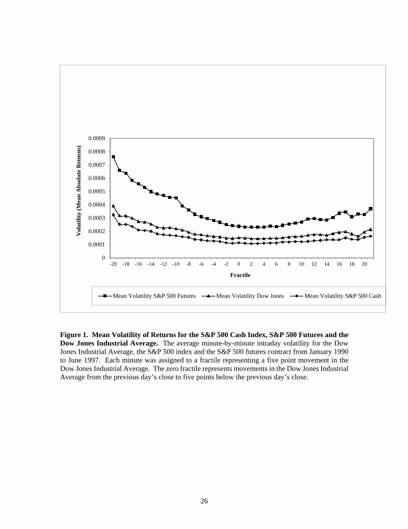
Figure 1. Mean Volatility of Returns for the S&P 500 Cash Index, S&P 500 Futures and the Dow Jones Industrial Average. The average minute-by-minute intraday volatility for the Dow Jones Industrial Average, the S&P 500 index and the S&P 500 futures contract from January 1990 to June 1997. Each minute was assigned to a fractile representing a five point movement in the Dow Jones Industrial Average. The zero fractile represents movements in the Dow Jones Industrial Average from the previous day’s close to five points below the previous day’s close.

0

0.0001

0.0002

0.0003

0.0004

0.0005

0.0006

0.0007

0.0008

0.0009

-20 -18 -16 -14 -12 -10 -8 -6 -4 -2 0 2 4 6 8 10 12 14 16 18 20

Vol

atili

ty (M

ean

Abs

olut

e R

etur

ns)

Fractile

Mean Volatility S&P 500 Futures Mean Volatility Dow Jones Mean Volatility S&P 500 Cash

26

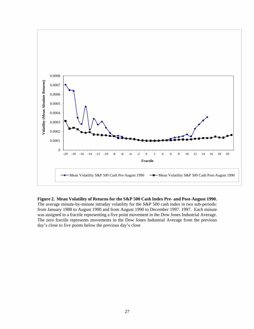
Figure 2. Mean Volatility of Returns for the S&P 500 Cash Index Pre- and Post-August 1990. The average minute-by-minute intraday volatility for the S&P 500 cash index in two sub-periods: from January 1988 to August 1990 and from August 1990 to December 1997. 1997. Each minute was assigned to a fractile representing a five point movement in the Dow Jones Industrial Average. The zero fractile represents movements in the Dow Jones Industrial Average from the previous day’s close to five points below the previous day’s close

0

0.0001

0.0002

0.0003

0.0004

0.0005

0.0006

0.0007

0.0008

-20 -18 -16 -14 -12 -10 -8 -6 -4 -2 0 2 4 6 8 10 12 14 16 18 20

Vol

atili

ty (M

ean

Abs

olut

e R

etur

ns)

Fractile

Mean Volatility S&P 500 Cash Pre-August 1990 Mean Volatility S&P 500 Cash Post-August 1990

27

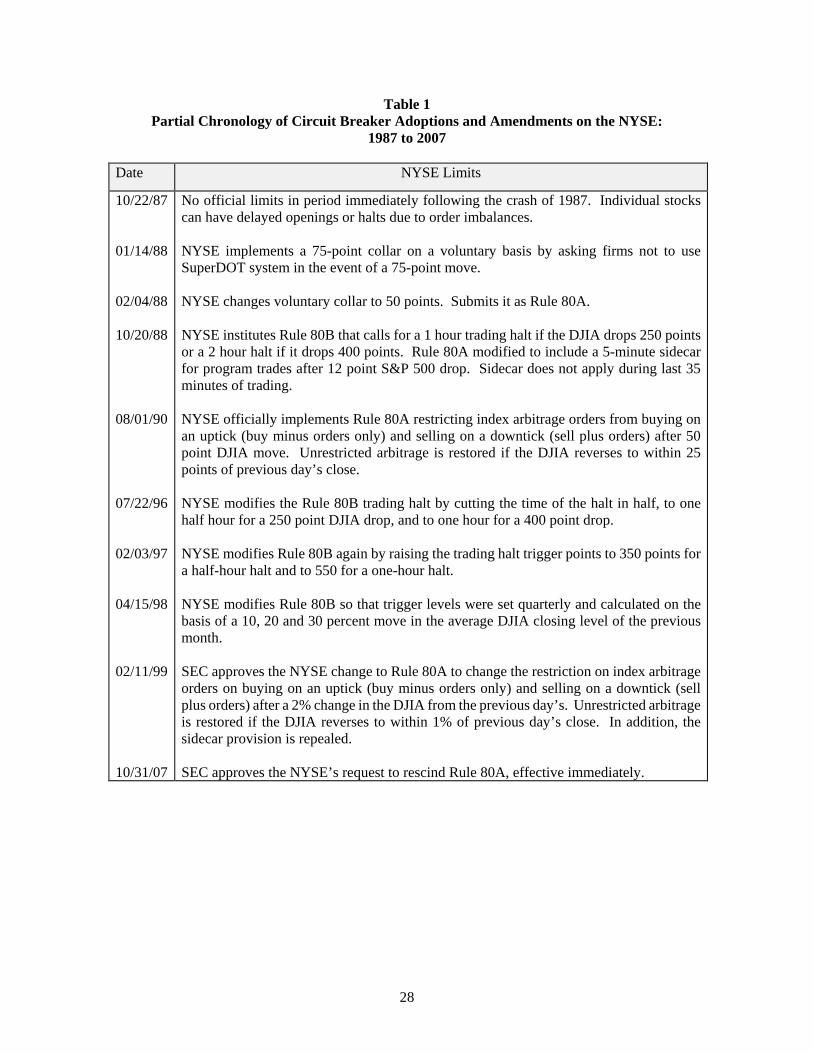
Table 1 Partial Chronology of Circuit Breaker Adoptions and Amendments on the NYSE:

1987 to 2007

Date NYSE Limits

10/22/87 01/14/88 02/04/88 10/20/88 08/01/90 07/22/96 02/03/97 04/15/98 02/11/99 10/31/07

No official limits in period immediately following the crash of 1987. Individual stocks can have delayed openings or halts due to order imbalances. NYSE implements a 75-point collar on a voluntary basis by asking firms not to use SuperDOT system in the event of a 75-point move. NYSE changes voluntary collar to 50 points. Submits it as Rule 80A. NYSE institutes Rule 80B that calls for a 1 hour trading halt if the DJIA drops 250 points or a 2 hour halt if it drops 400 points. Rule 80A modified to include a 5-minute sidecar for program trades after 12 point S&P 500 drop. Sidecar does not apply during last 35 minutes of trading. NYSE officially implements Rule 80A restricting index arbitrage orders from buying on an uptick (buy minus orders only) and selling on a downtick (sell plus orders) after 50 point DJIA move. Unrestricted arbitrage is restored if the DJIA reverses to within 25 points of previous day’s close. NYSE modifies the Rule 80B trading halt by cutting the time of the halt in half, to one half hour for a 250 point DJIA drop, and to one hour for a 400 point drop. NYSE modifies Rule 80B again by raising the trading halt trigger points to 350 points for a half-hour halt and to 550 for a one-hour halt. NYSE modifies Rule 80B so that trigger levels were set quarterly and calculated on the basis of a 10, 20 and 30 percent move in the average DJIA closing level of the previous month. SEC approves the NYSE change to Rule 80A to change the restriction on index arbitrage orders on buying on an uptick (buy minus orders only) and selling on a downtick (sell plus orders) after a 2% change in the DJIA from the previous day’s. Unrestricted arbitrage is restored if the DJIA reverses to within 1% of previous day’s close. In addition, the sidecar provision is repealed. SEC approves the NYSE’s request to rescind Rule 80A, effective immediately.

28

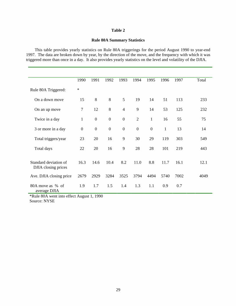
Table 2

Rule 80A Summary Statistics

This table provides yearly statistics on Rule 80A triggerings for the period August 1990 to year-end 1997. The data are broken down by year, by the direction of the move, and the frequency with which it was triggered more than once in a day. It also provides yearly statistics on the level and volatility of the DJIA.

Rule 80A Triggered:

1990

*

1991 1992 1993 1994 1995 1996 1997 Total

On a down move 15 8 8 5 19 14 51 113 233

On an up move 7 12 8 4 9 14 53 125 232

Twice in a day 1 0 0 0 2 1 16 55 75

3 or more in a day 0 0 0 0 0 0 1 13 14

Total triggers/year 23 20 16 9 30 29 119 303 549

Total days 22 20 16 9 28 28 101 219 443

Standard deviation of DJIA closing prices

16.3 14.6 10.4 8.2 11.0 8.8 11.7 16.1 12.1

Ave. DJIA closing price

2679 2929 3284 3525 3794 4494 5740 7002 4049

80A move as % of average DJIA

1.9 1.7 1.5 1.4 1.3 1.1 0.9 0.7

*Rule 80A went into effect August 1, 1990 Source: NYSE

29

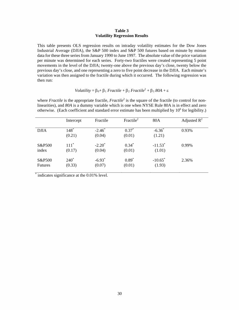
Table 3 Volatility Regression Results

This table presents OLS regression results on intraday volatility estimates for the Dow Jones Industrial Average (DJIA), the S&P 500 index and S&P 500 futures based on minute by minute data for these three series from January 1990 to June 1997. The absolute value of the price variation per minute was determined for each series. Forty-two fractiles were created representing 5 point movements in the level of the DJIA; twenty-one above the previous day’s close, twenty below the previous day’s close, and one representing a zero to five point decrease in the DJIA. Each minute’s variation was then assigned to the fractile during which it occurred. The following regression was then run:

Volatility = β0+ β1 Fractile + β2 Fractile2 + β3 80A + ε

where Fractile is the appropriate fractile, Fractile2 is the square of the fractile (to control for non-linearities), and 80A is a dummy variable which is one when NYSE Rule 80A is in effect and zero otherwise. (Each coefficient and standard error estimate has been multiplied by 106 for legibility.) Intercept Fractile Fractile2 80A Adjusted R2

DJIA 148* (0.21)

-2.46* (0.04)

0.37* (0.01)

-6.36* (1.21)

0.93%

S&P500 index

111* (0.17)

-2.20* (0.04)

0.34* (0.01)

-11.53* (1.01)

0.99%

S&P500 Futures

240* (0.33)

-6.93* (0.07)

0.89* (0.01)

-10.65* (1.93)

2.36%

* indicates significance at the 0.01% level.

30

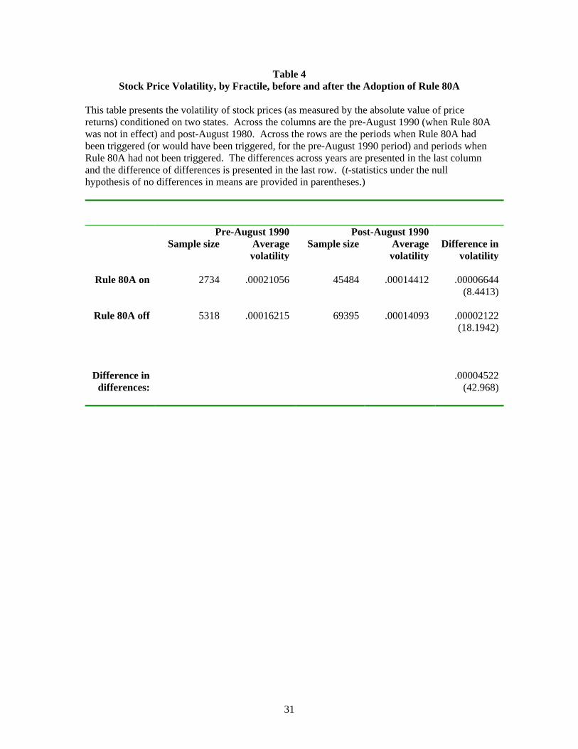
Table 4 Stock Price Volatility, by Fractile, before and after the Adoption of Rule 80A

This table presents the volatility of stock prices (as measured by the absolute value of price returns) conditioned on two states. Across the columns are the pre-August 1990 (when Rule 80A was not in effect) and post-August 1980. Across the rows are the periods when Rule 80A had been triggered (or would have been triggered, for the pre-August 1990 period) and periods when Rule 80A had not been triggered. The differences across years are presented in the last column and the difference of differences is presented in the last row. (t-statistics under the null hypothesis of no differences in means are provided in parentheses.)

Pre-August 1990 Post-August 1990 Sample size Average

volatility Sample size Average

volatility Difference in

volatility

Rule 80A on 2734 .00021056 45484 .00014412 .00006644 (8.4413)

Rule 80A off 5318 .00016215 69395 .00014093 .00002122

(18.1942)

Difference in differences:

.00004522 (42.968)

31

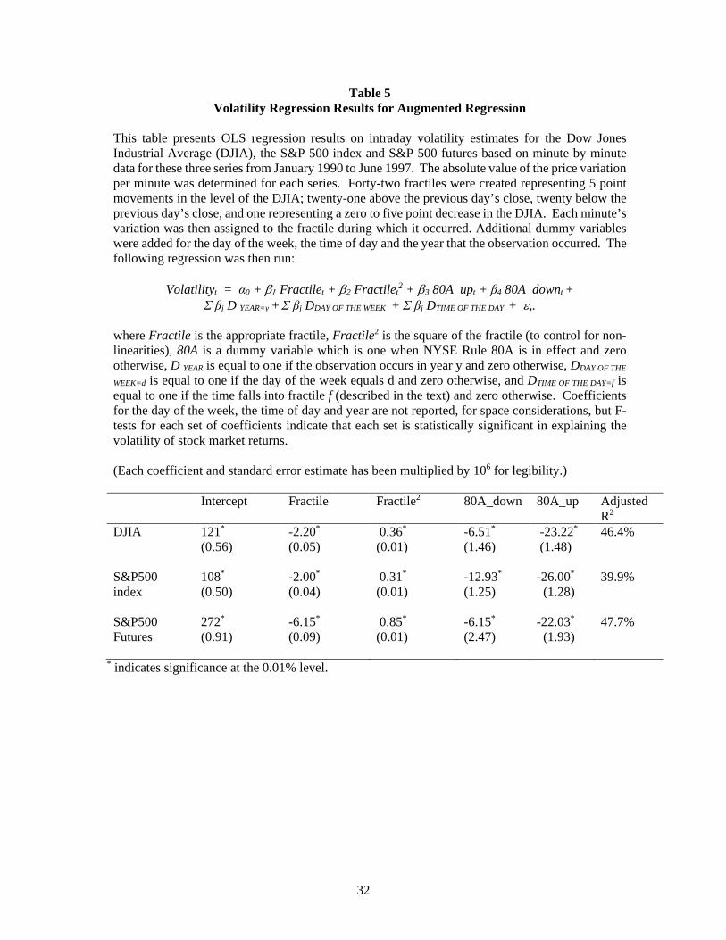
Table 5 Volatility Regression Results for Augmented Regression

This table presents OLS regression results on intraday volatility estimates for the Dow Jones Industrial Average (DJIA), the S&P 500 index and S&P 500 futures based on minute by minute data for these three series from January 1990 to June 1997. The absolute value of the price variation per minute was determined for each series. Forty-two fractiles were created representing 5 point movements in the level of the DJIA; twenty-one above the previous day’s close, twenty below the previous day’s close, and one representing a zero to five point decrease in the DJIA. Each minute’s variation was then assigned to the fractile during which it occurred. Additional dummy variables were added for the day of the week, the time of day and the year that the observation occurred. The following regression was then run:

Volatilityt = α0 + β1 Fractilet + β2 Fractilet2 + β3 80A_upt + β4 80A_downt +

Σ βj D YEAR=y + Σ βj DDAY OF THE WEEK + Σ βj DTIME OF THE DAY + ε,.

where Fractile is the appropriate fractile, Fractile2 is the square of the fractile (to control for non-linearities), 80A is a dummy variable which is one when NYSE Rule 80A is in effect and zero otherwise, D YEAR is equal to one if the observation occurs in year y and zero otherwise, DDAY OF THE

WEEK=d is equal to one if the day of the week equals d and zero otherwise, and DTIME OF THE DAY=f is equal to one if the time falls into fractile f (described in the text) and zero otherwise. Coefficients for the day of the week, the time of day and year are not reported, for space considerations, but F-tests for each set of coefficients indicate that each set is statistically significant in explaining the volatility of stock market returns. (Each coefficient and standard error estimate has been multiplied by 106 for legibility.) Intercept Fractile Fractile2 80A_down 80A_up Adjusted

R2

DJIA 121* (0.56)

-2.20* (0.05)

0.36* (0.01)

-6.51* (1.46)

-23.22* (1.48)

46.4%

S&P500 index

108* (0.50)

-2.00* (0.04)

0.31* (0.01)

-12.93* (1.25)

-26.00* (1.28)

39.9%

S&P500 Futures

272* (0.91)

-6.15* (0.09)

0.85* (0.01)

-6.15* (2.47)

-22.03* (1.93)

47.7%

* indicates significance at the 0.01% level.

32