Embed Size (px)
Citation preview

Citation: Kamjoo, Azadeh (2015) A Decision Support System for Integrated Design of Hybrid Renewable Energy System. Doctoral thesis, Northumbria University.
This version was downloaded from Northumbria Research Link: http://nrl.northumbria.ac.uk/27224/
Northumbria University has developed Northumbria Research Link (NRL) to enable users to access the University’s research output. Copyright © and moral rights for items on NRL are retained by the individual author(s) and/or other copyright owners. Single copies of full items can be reproduced, displayed or performed, and given to third parties in any format or medium for personal research or study, educational, or not-for-profit purposes without prior permission or charge, provided the authors, title and full bibliographic details are given, as well as a hyperlink and/or URL to the original metadata page. The content must not be changed in any way. Full items must not be sold commercially in any format or medium without formal permission of the copyright holder. The full policy is available online: http://nrl.northumbria.ac.uk/policies.html
A Decision Support System for
Integrated Design of Hybrid Renewable
Energy System
A KAMJOO
PhD
2015
A Decision Support System for
Integrated Design of Hybrid Renewable
Energy System
AZADEH KAMJOO
A thesis submitted in partial fulfilment
of the requirements of the
University of Northumbria at Newcastle
For the degree of
Doctor of Philosophy
Research undertaken in the Faculty of
Engineering and Environment
February 2015
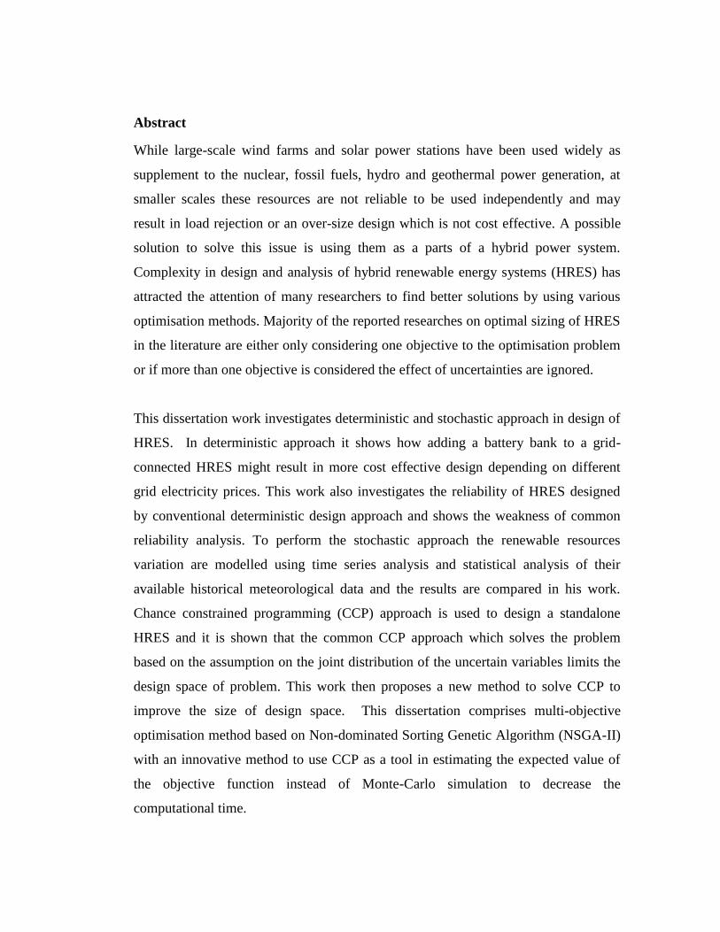
Abstract
While large-scale wind farms and solar power stations have been used widely as
supplement to the nuclear, fossil fuels, hydro and geothermal power generation, at
smaller scales these resources are not reliable to be used independently and may
result in load rejection or an over-size design which is not cost effective. A possible
solution to solve this issue is using them as a parts of a hybrid power system.
Complexity in design and analysis of hybrid renewable energy systems (HRES) has
attracted the attention of many researchers to find better solutions by using various
optimisation methods. Majority of the reported researches on optimal sizing of HRES
in the literature are either only considering one objective to the optimisation problem
or if more than one objective is considered the effect of uncertainties are ignored.
This dissertation work investigates deterministic and stochastic approach in design of
HRES. In deterministic approach it shows how adding a battery bank to a grid-
connected HRES might result in more cost effective design depending on different
grid electricity prices. This work also investigates the reliability of HRES designed
by conventional deterministic design approach and shows the weakness of common
reliability analysis. To perform the stochastic approach the renewable resources
variation are modelled using time series analysis and statistical analysis of their
available historical meteorological data and the results are compared in his work.
Chance constrained programming (CCP) approach is used to design a standalone
HRES and it is shown that the common CCP approach which solves the problem
based on the assumption on the joint distribution of the uncertain variables limits the
design space of problem. This work then proposes a new method to solve CCP to
improve the size of design space. This dissertation comprises multi-objective
optimisation method based on Non-dominated Sorting Genetic Algorithm (NSGA-II)
with an innovative method to use CCP as a tool in estimating the expected value of
the objective function instead of Monte-Carlo simulation to decrease the
computational time.

To my Father
I
Table of Contents Declaration ................................................................................................................ VII
Acknowledgement.................................................................................................... VIII
Nomenclature and Abbreviations ................................................................................ IX
1 Introduction ............................................................................................................ 1
1.1 Need for Renewable Energy ........................................................................... 2
1.2 Hybrid Renewable Energy Systems ............................................................... 2
1.3 Design Decision Support System ................................................................... 3
1.4 Optimal Sizing of HRES ................................................................................ 5
1.5 Optimisation Methods .................................................................................... 7
1.5.1 Particle swarm optimisation .................................................................... 7
1.5.2 Simulated annealing ................................................................................ 8
1.5.3 GA ........................................................................................................... 8
1.5.4 NSGA-II ................................................................................................ 16
1.5.5 Other optimisation methods reported in literature ................................ 19
1.6 Available Software Tools for Sizing HRES ................................................. 20
1.7 Deterministic and Stochastic Design Approaches ........................................ 23
1.7.1 Determinstic design approach and problem formulation ...................... 23
1.7.2 Stochastic design approach ................................................................... 25
1.8 Scope of thesis and contribution to the knowledge ...................................... 33
1.9 Structure of this thesis .................................................................................. 36
2 Modelling ............................................................................................................. 38
2.1 HRES components ....................................................................................... 39
2.1.1 Wind Turbines ....................................................................................... 39
2.1.2 Wind Turbine Model ............................................................................. 40
2.1.3 Photovoltaic Panels ............................................................................... 43
2.1.4 Photovoltaic(PV) Panel Model ............................................................. 45
2.1.5 Storage System ...................................................................................... 47
2.1.6 Battery bank Model ............................................................................... 47

II
2.1.7 Battery lifetime...................................................................................... 49
2.1.8 Economic Analysis................................................................................ 50
2.1.9 Income Modelling ................................................................................. 51
2.1.10 Cost Modelling ...................................................................................... 51
3 Optimal sizing of grid-connected hybrid wind-PV systems with battery bank ... 55
3.1 Introduction .................................................................................................. 56
3.2 Economic analysis ........................................................................................ 57
3.3 Problem formulation & design scenarios ..................................................... 58
3.4 Case study ..................................................................................................... 63
3.5 Results .......................................................................................................... 64
3.6 Summary ...................................................................................................... 71
4 Reliability of Deterministic Design Approach ..................................................... 72
4.1 Introduction .................................................................................................. 73
4.2 Problem formulation and design methodology ............................................ 74
4.3 Case study ..................................................................................................... 76
4.4 Results and Discussion ................................................................................. 78
4.5 Summary ...................................................................................................... 81
5 Stochastic design approach in optimal sizing of HRES ...................................... 82
5.1 Introduction .................................................................................................. 83
5.2 The wind speed and solar irradiance simulation model ............................... 85
5.2.1 Problem formulation and design methodology ..................................... 85
5.2.2 Case study ............................................................................................. 86
5.2.3 Results and Discussion .......................................................................... 88
5.2.4 On the Sensitivity Analysis ................................................................... 90
5.2.5 Summary ............................................................................................... 91
6 Chance Constrained Programming Using Non-Gaussian Joint Distribution
Function in Design of Standalone Hybrid Renewable Energy Systems ..................... 92
6.1 Introduction .................................................................................................. 93
6.2 Problem formulation and design methodology ............................................ 96
6.2.1 Common method used in previous studies-Using normal distribution . 98
III
6.2.2 The proposed method ............................................................................ 99
6.3 Case study ................................................................................................... 100
6.4 Validation with Monte Carlo simulation .................................................... 104
6.5 Summary .................................................................................................... 106
7 Multi-Objective Design under Uncertainties of Hybrid Renewable Energy
System Using NSGA-II and Chance Constrained Programming ............................. 114
7.1 Introduction ................................................................................................ 115
7.2 Problem formulation and design methodology .......................................... 118
7.3 Optimal Estimation of the Objective Functions Affected by Uncertainties
Using CCP ............................................................................................................. 120
7.4 Monte Carlo Simulation ............................................................................. 121
7.5 Case study ................................................................................................... 122
7.6 Results and discussion ................................................................................ 123
7.7 Summary .................................................................................................... 131
8 Summary and Conclusion .................................................................................. 133
8.1 Original contribution .................................................................................. 134
8.1.1 Design of grid-connected HRES considering a back-up storage ........ 134
8.1.2 Investigation on the reliability of deterministic design approach ....... 135
8.1.3 Modelling the variation of power coefficient of the wind turbine ...... 135
8.1.4 Modelling the uncertainties of renewable resources ........................... 135
8.1.5 Optimal design of HRES under uncertainties using CCP ................... 136
8.1.6 Multi objective optimal design of HRES under uncertainties ............ 136
8.2 Critical appraisal and future works............................................................. 137
List of Publications ................................................................................................... 138
References ................................................................................................................. 139
IV
List of Figures Figure 1-1 Concept diagram of HRES ........................................................................ 35
Figure 1-2 Summer and winter load profiles .............................................................. 36
Figure 2-1 Wind Turbine Configurations ................................................................... 40
Figure 2-2 Cp curves of different wind turbines in the range of kW1 to kW15 ....... 44
Figure 2-3 Principles of PV energy conversion ......................................................... 45
Figure 2-4 Battery’s lifetime vs. DOD ........................................................................ 50
Figure 3-1 Average Hourly Solar Irradiance: ............................................................. 61
Figure 3-2 Average Hourly Wind Speed .................................................................... 62
Figure 3-3 PV Area vs. HRES Performance and Cost ............................................... 64
Figure 3-4 share vs. Peak Hour Price Rate ................................................................ 65
Figure 3-5 comparison between two best solutions of three different Peak prices ..... 68
Figure 3-6 The produced power of each source for typical months ........................... 70
Figure 4-1 Average Hourly Solar Irradiance .............................................................. 76
Figure 4-2 Average Hourly Wind Speed .................................................................... 77
Figure 4-3 Typical Day with Power Shortage............................................................. 79
Figure 4-4 State of Charge of the Battery Bank .......................................................... 79
Figure 4-5 State of Charge of the Battery Bank after considering maximum blackout
hours in design ............................................................................................................ 80
Figure 5-1 Block diagram of applying time analysis on historical weather data ........ 84
Figure 5-2 An example of simulated wind speed........................................................ 87
Figure 5-3 An example of simulated solar irradiance ................................................. 87
Figure 5-4 Upper & lower DPSP for design candidates ............................................. 89
Figure 5-5 DPSP values of optimum solution ............................................................ 89
Figure 5-6 Distribution of DPSP values for optimum solution .................................. 90
Figure 5-7 Probability of blackout occurrence for each day of year........................... 90
Figure 6-1 Block diagram of proposed design method and validation process ........ 103
Figure 6-2 Contour plot of joint probability of WT and PV panel output powers for
Aug at 12:00 .............................................................................................................. 107

V
Figure 6-3 The total cost of optimum solutions of two methods for different
confidence levels ....................................................................................................... 108
Figure 6-4 The design spaces of two methods for α=0.8 .......................................... 108
Figure 6-5 Feasible design solutions & selected optimum solution of optimisation
problem Eq. 6.14- Using proposed method for α=0.8 .............................................. 109
Figure 6-6 Feasible design solutions & selected optimum solution of optimisation
problem Eq. 6.14- Using normal dist. for α=0.8 ....................................................... 109
Figure 6-7 Mean values of simulated and observed data of wind speed .................. 110
Figure 6-8 Error values of simulated and observed data of wind speed ................... 110
Figure 6-9 Mean values of simulated and observed data of solar irradiance ............ 111
Figure 6-10 Error values of simulated and observed data of solar irradiance .......... 111
Figure 6-11 Deficiency of power supply probability of optimum solution obtained
with Monte Carlo simulation .................................................................................... 112
Figure 6-12 Comparison between probability of blackout occurrences of two
optimum solutions for α=0.8 ..................................................................................... 112
Figure 6-13 Comparison between average daily power excess of two optimum
solutions for α=0.8 .................................................................................................... 113
Figure 7-1.NSGA-II with chance constrained programming .................................... 124
Figure 7-2 NSGA-II with Monte Carlo simulation ................................................... 125
Figure 7-3 Comparison of Pareto sets obtained with different optimisation methods
................................................................................................................................... 126
Figure 7-4 Monte-Carlo simulation results on optimum solution of NSGA-II with
chance constrained programming for reliability=0.8 ................................................ 129
Figure 7-5 Monte-Carlo simulation results on optimum solution of NSGA-II with
Monte Carlo simulation for reliability=0.8 ............................................................... 131

VI
List of Tables Table 1-1 Components design parameters .................................................................. 36
Table 3-1 The battery bank specification .................................................................... 63
Table 3-2 Grid electricity process in UK .................................................................... 63
Table 3-3 Optimum configuration of each price rate .................................................. 66
Table 4-1 Optimum solution based on common design method ................................ 77
Table 4-2 Optimum solution after adding constraint on maximum blackout hours ... 80
Table 5-1 Optimum Configuration.............................................................................. 88
Table 6-1 The comparison between results obtained using two design methods .... 102
Table 7-1 Monte Carlo simulation parameters.......................................................... 122
Table 7-2 Optimum solutions of two design methods for reliability=0.8 ................. 127

VII
Declaration
I declare that the work contained in this thesis has not been submitted for any other
award and that it is all my own work. I also confirm that this work fully
acknowledges opinions, Ideas and contribution from work of others.
Name: Azadeh Kamjoo
Signature:
Date:

VIII
Acknowledgement
I would like to sincerely thank Dr. Alireza Maheri for his guidance, encouragements,
trust and constructive advices during my research at Northumbria University.
I also deeply thank Prof. Ghanim Putrus, as my second supervisor for being very
supportive and patient throughout the research.
For this work, I also would like to thank Northumbria University and Synchron
Technology Ltd., for the financial support of the project.
Azadeh Kamjoo
Newcastle upon Tyne

IX
Nomenclature and Abbreviations
confidence level
t the time step (one hour in this study)
PV efficiency of the PV array and corresponding converters
Bat battery efficiency
Mean
standard deviation
air density (1.225 Kg/m3)
PVA PV panel area (m2)
WTA wind turbine rotor disk area (m2)
0C total constant cost including the cost of installation of the wind turbine
and PV panels ($)
BatC nominal battery bank capacity (Ah)
ICC the total cost of the system($)
MOC & present value of maintenance cost ($)
repC the present value of replacement cost ($)
BatUnitC , unit Cost of battery bank ($/Ah)
PVUnitC , unit Cost of PV panel ($/m2)
WTUnitC , unit cost of the wind turbine($/m2)
pC wind turbine power coefficient,
1F inverse of the joint cumulative distribution function
I horizontal solar irradiance in (W/m2)
BatI battery current (A)
dk annual real interest rate (%)
X
pL system life period (years)
BatN total number of batteries
repN number of replacements of the battery over the system life period
BatP battery bank available power (W)
PVP the PV array output power (W)
WTP wind turbine power (W)
NomPVP , PV panel nominal power (W)
SOC state of the charge of the battery
TC the total cost of the system ($)
BatV battery voltage (V)
Z inverse of the cumulative normal probability distribution
ARMA auto-regressive moving average
DOD depth of discharge
DPSP deficiency of power supply probability
GA genetic algorithm
HRES hybrid renewable energy systems
LPSP loss of power supply probability
MSE mean squared error
IINSGA non-dominated sorting genetic algorithm
PSO particle swarm optimisation
RSM response surface methodology
SA simulated annealing
TS Time Series

1
1 Introduction

2
1.1 Need for Renewable Energy
A great part of energy supply of the today world is provided from conventional
energy resources. These energy resources are finite and fast depleting and are
provided at a very high cost [1]. At the same time the energy demand around the
world is increasing exponentially and conventional energy resources would not be
able to supply it for long. In addition to high cost and the limitations in supply
resources of conventional energy resources, their negative impact on environment and
global warming have attracted the attention to other alternative power sources those
are environmental friendly, reliable and cost effective. Renewable resources appear to
be one of the most sustainable energy resources available. Wind energy, solar energy,
biomass, hydropower, ocean tidal and wave energy are examples of renewable energy
resources. Renewable energy sources can particularly be the best electricity provider
in small scale applications such as street lighting, household electricity and also
energy supply for remote places and islands [2-4]. Using renewable energy resources
can decrease the cost of transmission and transformational costs although common
drawback of using renewable resources is constant challenge with their unpredictable
nature which is completely dependent on climate changes and may result in load
rejection at some points [5]. A possible solution to solve this issue is using them as a
parts of a hybrid power system.
1.2 Hybrid Renewable Energy Systems
Hybrid renewable energy systems (HRES) combine two or more renewable energy
sources to generate power [6-8] such that each of them can cover the weakness of
another one in load demand coverage and the power generation system can provide
continuous power supply in various weather statuses and potentially improves the
system efficiency and reliability of power supply [9-11]. Obviously the combination
of different renewable resources needs to be adapted based on the conditions of each
specified location.

3
The hybrid power systems can be designed as the stand-alone or grid-connected
systems. Many parameters such as attainable power from grid, cost of providing
power from grid and individual meteorological characteristic of the desired site. The
grid-connected systems are designed in the way that they are able to cover their local
demand and depending on the grid capacity, the excess produced power can be sold
to the grid to be transferred to other places of demand. Additionally in case of power
shortage in the production of renewable resources the remaining required power can
be provided by grid thus these systems do not require a separate storage system to
maintain the reliability because the grid will perform as an infinite backup system.
On the other hand, stand-alone hybrid renewable systems are the most promising
solution to bring electricity to remote places. However since there is no grid
connection available for these systems they require to have a backup or auxiliary unit
such as battery banks or conventional diesel generators for assistance in maintaining
the reliability.
In both grid connected or stand-alone cases, investment costs of providing electricity
from renewable sources and reliability of the designed system are usually problems
with main importance in long term planning of energy systems and as a result
selecting the best renewable energy resource; optimal solution among different
possible combination of renewable energy sources is important. Depending on the
number of objectives a single-objective or multi-objective problem is defined to find
the optimal solution or a set of trade-off solutions in design of HRES for decision
making.
1.3 Design Decision Support System
As mentioned before hybrid renewable energy systems have been proved as a viable
solution to bring electricity to remote places where it is expensive or impossible to
extend the grid. Considering that the renewable power generators are reliant on the
climate conditions which makes them inherently intermittent, the fact that these
4
systems either need to be able to provide electricity without the support of grid
connection and maintain the certain reliability if stand-alone or the cost-effectiveness
of produced power for grid-connected systems, can sometimes result in overdesign of
these systems or the outcome may become less efficient economically. The goal of
providing electricity from combining renewable resources at a reasonable cost and
reliability, optimal design of HRES in terms of operation and combination of the
components is essential[12] . Complexity in design and analysis of hybrid renewable
energy systems has attracted the attention of many researchers to find better solutions
in the design of HRES, which mostly are focused on cost reduction and efficiency
improvement of these systems [13].
In the design process there are often more than one alternative for each design
component and there are many design possibilities to be considered and evaluated.
This is the main reason for optimisation process and providing quantitative
assessment of different design solution to support and facilitate the decision making
process [14-16]. Decision making problems can be categorized to two classes based
on the number of objective functions that are involved in the problem; single
objective and multi-objective. In a single objective problem the aim is to identify the
best solution corresponding to minimising or maximising a single objective function.
However many real world decision making processes involve more than one
objective function at the same time like minimising cost and maximising the
reliability. Clearly this category of problems does not have a single solution
achieving contradicting objectives. That is why multi-objective problems do not have
a single optimal solution but they have a set of compromised solutions between
different objective functions known as Pareto sets. Providing a set of solutions to an
optimisation problem introduces three major advantages [17] a wider set of solutions
are identified; selecting between different alternatives enquires the necessity of an
analyst to produce different solutions and the decision maker to evaluate the solutions
provided by the analyst and make decisions; models of a problem would be more
realistic by considering several objectives. However, multi objective problems can be

5
changed to a single objective problem by integrating multiple objectives in one or by
considering an objective as main objective and the rest as design constraints.
However in this approach the analyst makes most of the decisions by deciding the
weight that each of the multiple objectives would have in the integrated single
objective or by the level of compromise he defines for the design objectives as
constraints. This approach would take away the evaluation and deciding between
different alternatives from the decision maker. On the other hand the interaction
between different objectives yields to a set of design candidates known as Pareto-
optimal solutions. The main characteristic of Pareto set members is that they are not
dominated by other solutions, meaning that it is not possible to improve on one
objective without worsening another objective function.
In optimal design of HRES several objectives need to be optimised, most of them
contradicting (e.g. cost & reliability), therefore in design of HRES a multi-objective
optimisation approach should be followed. However selection among design
candidates is subjective and depends on decision maker’s judgement, which in turn
depends on his knowledge, background. A Design Decision Support System (DDSS)
is required to help decision makers to choose among different design alternatives.
This is achievable by taking into account all the technical & economic considerations
and providing the user with facilities like sorting, filtering, and visual figures to
compare and finally select the more suitable design.
1.4 Optimal Sizing of HRES
Designing a power generation plant is very important from economic, environmental
and quality of production point of view. Considering the worldwide increase in
energy demand, increasing the capacity of existing grid networks or adding new
micro grids has become a problem of interest in many aspects. The unavoidable
discontinuity in the generation of power production systems with a single renewable
resource has caused design of HRES more popular in the recent years. Despite of the

6
number of research reported in design of HRES, the majority of them are considering
a single objective. Garcia and Weisser [18] compared two models to determine the
optimal size of wind-diesel power system with hydrogen storage in a grid-connected
system. Both models are designed with considering either the cost or reliability as the
main objective. Design of HRES for remote place makes the system availability the
main objective rather than the cost. In this case finding the proper storage system is
also considered to maintain desired availability. Balamurugan et al. [19] optimised a
hybrid power system of wind, biomass, solar photovoltaic with battery bank storage
considering availability as the main objective. The hybrid energy system is sized
considering a suitable storage system to provide the power at periods when there is no
solar power available or during minimum wind speed periods.
As mentioned two important contradictory objective functions in optimal sizing of
HRES are usually cost and reliability and since these objectives are contradicting a
single optimal solution cannot be found with minimum cost and maximum reliability
and multi-objective optimisation should be performed to find the trade-off set; Pareto
set of the solutions. Many studies have been reported in multi-objective optimisation
of HRES considering different objection functions, using various optimisation
techniques. Katsigiannis [20] used a multi-objective algorithm to minimise the cost
of produced power of the system and total green house gas emission during the
system. Kaabeche, Belhamel and Ibtiouen [21] recommended an optimisation model
based on iterative technique to optimise the size of hybrid wind/photovoltaic system
combining with a battery bank minimising het deficiency of power supply and
levelised unit electricity cost. However, despite the claim of considering more than
one objective in design of HRES in mentioned studies, they are in fact single
objective, as either objectives are not contradicting or all-but-one are treated as
constraints.

7
1.5 Optimisation Methods
This section briefly explains some of the optimisation methods used in design of
HRES.
1.5.1 Particle swarm optimisation
Particle swarm optimisation (PSO) is a population-based stochastic optimisation
technique in evolutionary computation. This technique was developed in 1995 by
Kennedy and Eberhart and is based on movement of swarms, looking for food. Each
potential solution to the optimisation problem is called a particle and the co-ordinates
of each particle are defined by its velocity vector and its position. Initially each
particle is flown through the search space at a random velocity. Assuming that the
population have good knowledge about other particles and their own position, at each
iteration the particles examine the search area, modify their velocity and move
towards the best solution among them. Since all the particles in the population follow
the same approach at each iteration a group movement toward the optimum solution
is reached. The process continues until the constraint on the maximum iteration is
reached.
The implementation of PSO is based on simple equations and thus the process time is
short and efficient however since the movement of the particles in three directions
coordinates with the number of design variables, where there are more than three
design variables it would be more suitable to use another optimisation technique.
Mahor et al. [22] applied particle swarm optimisation to solve same problem
concluding that the proposed PSO method had better performance comparing to the
conventional optimisation techniques. Kaviani et al. [23] used a PSO to optimise a
hybrid photovoltaic-wind-fuel cell generation system minimising the annual cost of
the hybrid system providing desired reliability in maintain the load demand. More
samples in use of PSO can be addressed in [24-26].
8
1.5.2 Simulated annealing
The simulated annealing (SA) process is a general optimisation technique which was
first introduced by Kirkpatrick et al [27]. At each iteration of the SA process, a
candidate move is selected randomly and this move is evaluated. If the move leads to
a better solution which means the new solution has better fitness value then the move
is accepted otherwise it might be rejected with a probability that depends on the
difference between its fitness value and the best fitness value. The annealing process
based on decreasing the temperature allows wider search area by choosing faster
temperature decrement at the start of the iteration process and slower temperature
decrement to reach the local search in the next iterations. The cooling schedule
procedure is the main structure of the SA method. SA method has not been very
popular in the design of HRES. Giannakoudis et al. [28] performed an optimisation
method based on SA to design and operate a hybrid power generation system that
includes wind turbine, photo voltaic panels, , hydrogen storage tanks, a compressor, a
fuel cell and a diesel generator.[29-31] can be referred as they have also worked
based on SA.
1.5.3 GA
Genetic Algorithm (GA) is developed based on biological principles of genetics. GA
was first introduced by Holland [32] and has been widely used in solving
optimisation problems in variety of real world problems in different research areas.
Following the biological process, such as crossover, and mutation in the optimisation
process, GA is capable of solving complex real world problems [33]. The algorithm
starts by creating a “Population” of “chromosomes” which are randomly generated
and each can be possible solution to the optimisation problem. Each “Chromosome”
is measured against the value of the objective function and assigned a value of
“Fitness” and the least favourable chromosomes in terms of fitness would be
discarded. At each generation the chromosomes are sorted and some are selected as
the parents to “Crossover” and form offspring. The offspring might replace the
parents in case they have better characteristics; better fitness value. Another

9
important biological operator in genetic algorithm is “Mutation”. At each generation
a number of chromosomes undergo mutation in which essentially a random section of
chromosome is changed to generate a different chromosome. The process of
implementing crossover, mutation operators and selection on chromosomes are
iterated until the population is converged and the optimal solution is found or the
maximum number of generation is reached. The main advantage of the GA is that it
can easily jump out of a local optima and reach the global optima. Unlike PSO
method GA does not put any limit on the number of design variables however it
might be more challenging to implement the GA code.
Genetic algorithm may not always be the quickest way to find the optimum solution,
when it comes to complex problems with many constraints; it is a very effective
method to solve the problem. Overall advantages that GA has over other optimisation
methods have attracted many researchers to use GA in reported researched in design
of HRES [34-40]. Ould et al. [41] proposed a real multi-objective GA in optimal
sizing of a hybrid wind-solar-battery system with the objective of minimising the
yearly cost system and the loss of power supply probability. However the effect of
uncertainties in renewable resources is ignored in this research. Yang et al.
[42]proposed optimal sizing method based on GA technique using the Typical
Meteorological Year data. This proposed optimisation model calculates the system
optimum configuration which is able of achieving the desired LPSP with minimum
Annualized Cost of System.
The genetic algorithm follows below steps.
Generate initial population
As described the population consists of a number of members, chromosomes that
each have the possibility to be a solution to the optimisation problem. A chromosome
is made up by the design variables.

10
The initial population is generated randomly by selecting a random value for each
design variable between defined bounds using below equation.
).( lhl vvvv (1.1)
where v would be the random value of the design variable, a randomly generated
number between 0 and 1. lv , hv are the lower and higher bound of the design
variable respectively.
Crossover
Crossover is the main genetic operator in the genetic algorithm. This operator
operates on a pair of chromosomes, combines parts of the parent chromosomes
features to produce offspring. To perform this operator two individuals are randomly
selected from sampling pool. The number of individuals undergoing the crossover is
determined by crossover probability cp . A high crossover probability allows
exploration on more solution space which reduces the chance of convergence of the
algorithm to a local optimum. Although choosing a very high crossover probability
would increase the computation time in exploring unpromising regions of solution
space [43].
a)N-point crossover: This form of crossover is the simplest form of crossover.
According to it, based on the number of cut points the parents are divided to the
different segments those would be exchanged to form new individuals (children). The
number of cut point can be chosen randomly however it cannot exceed the number of
control variables.
b)Uniform crossover: in this method each gene of the child would be randomly
selected between the respective genes of the parents. The genes of both parents would
have equal chance to be selected as genes of the child.
11
c)Arithmetical crossover: This type of crossover is defined as a linear combination
of vectors and is very useful in real representation. Below equations represent the
arithmetical crossover:
211 )1(. ParentParentchild (1.2)
122 )1(. ParentParentchild (1.3)
where is a random number between 0 and 1.
d)Blend crossover: This type of crossover is the most common form of
recombination and is the general form of arithmetical crossover. It can be expressed
using below equations.
211 )1(. ParentParentchild (1.4)
212 ).1( ParentParentchild (1.5)
and is determined as:
u)21( (1.6)
where u is a random number generated for each gene with uniform distribution in the
interval of 0 and 1. Parameter is chosen as a once for all the genes and its value
changes between 0 and 1.
If is set as 0 the blend crossover would work as arithmetical crossover.
Mutation
Unlike crossover the mutation operator aims in producing new individual from only
one parent. By making spontaneous changes to the structure of chromosome the
mutation operator introduces new solution to the optimisation problem. A simple way
to implement the mutation operator would be to alter one or two genes in the
12
chromosome. Every gene in the structure of the parent chromosome has equal chance
to be mutated. This operator serves the GA by introducing new genes to the set of
solution that might have been lost through the selection process or have not been
presented in the initial population. Similar to crossover probability, mutation
probability defines the percentage of the population that would undergo the mutation.
However choosing a proper value for mutation rate is very important as if it is very
low many new genes that might be useful would not be introduced to the solutions
and if it is very high the offspring would lose their resemblance to their parents and
the algorithm would lose the ability of learning from the past of the search.
Selection
In Holland’s original GA [32] selection was referred to choosing parents to
recombination and in that method the parents where always been replaced by their
produced offspring despite of the possibility that offspring might be less fitter than
the parents. With this strategy might result in losing some fitter chromosomes [43].
Although the term Selection is also used to form new generation [44]. Generally
selection is implemented two times in genetic algorithms: selection for reproduction
and selection for next generation.
a)Selection for reproduction
This kind of selection is performed to choose the chromosomes within the current
population those would be taken to reproduction. There are three selection methods;
roulette wheel, rank based and tournament selection and all of them use the
chromosomes fitness values to perform the selection process. The selected
individuals would be added to a sampling pool.
Roulette-wheel selection
This selection method is a proportionate selection based on the fitness value. All the
individuals of the population would have the chance of being selected. This method is

13
emphasized to the fitter individuals in the population and the individuals with lower
fitness value would have slimmer chance to be selected. At the population with
popn chromosomes, each individual of ix with the fitness of )( ixfitness is assigned a
probability of selection which is calculated as:
popn
ii
i
xfitness
xfitnessi
1
)(
)()Pr( (1.7)
In this method the chance of an individual being selected is proportional to the value
of its probability of selection. The advantage of this method is that it does not discard
any of the chromosomes in the selection process and gives the chance however the
chromosomes with higher fitness value would occupy bigger segment in the wheel
and would have higher chance of being selected. This might cause the diversity of the
population to decrease and the algorithm to converge to a local optima point. A
sample procedure of implementing roulette-wheel selection is shown below:
While sampling pool is full
Number=Random number (0, 1)
For each member in population
If Number>Fitness (member) select member
End for
End
Rank-based selection
Rank-based selection is another form of proportionate selection. In this method the
rank of the chromosomes is used to calculate the selection probability. This method
gives higher chance to the individuals with lower fitness to be chosen and participate
in reproduction process which could help to prevent the algorithm from premature
convergence.
14
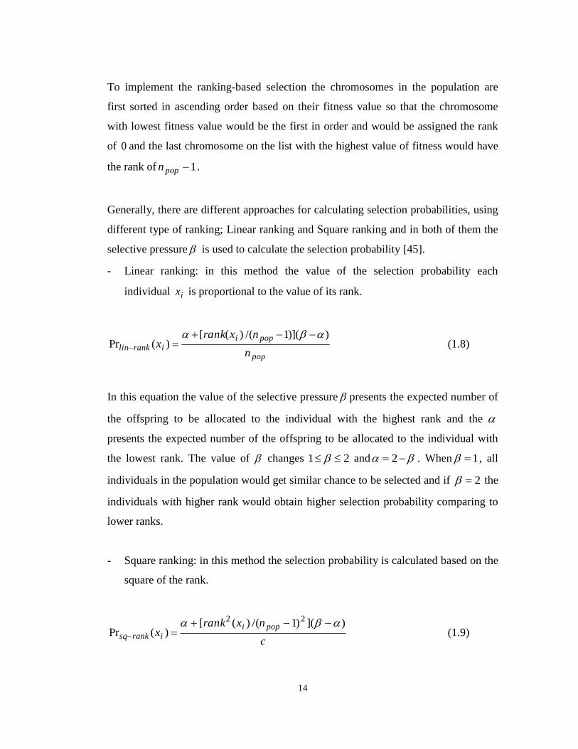
To implement the ranking-based selection the chromosomes in the population are
first sorted in ascending order based on their fitness value so that the chromosome
with lowest fitness value would be the first in order and would be assigned the rank
of 0 and the last chromosome on the list with the highest value of fitness would have
the rank of 1popn .
Generally, there are different approaches for calculating selection probabilities, using
different type of ranking; Linear ranking and Square ranking and in both of them the
selective pressure is used to calculate the selection probability [45].
- Linear ranking: in this method the value of the selection probability each
individual ix is proportional to the value of its rank.
pop
popiiranklin
n
nxrankx
))](1/()([)(Pr
(1.8)
In this equation the value of the selective pressure presents the expected number of
the offspring to be allocated to the individual with the highest rank and the
presents the expected number of the offspring to be allocated to the individual with
the lowest rank. The value of changes 21 and 2 . When 1 , all
individuals in the population would get similar chance to be selected and if 2 the
individuals with higher rank would obtain higher selection probability comparing to
lower ranks.
- Square ranking: in this method the selection probability is calculated based on the
square of the rank.
c
nxrankx
popiiranksq
)]()1/()([)(Pr
22 (1.9)
15
Similar to linear ranking the value of changes 21 however here the value
of is arbitrary choosing in the boundaries 0 . Normalization factor c is
calculated as:
poppoppoppop nnnnc )1(6/)12()( (1.10)
In both linear and square ranking methods, after calculating the selection probability
the sampling process to choose individuals is done using roulette-wheel selection.
Tournament selection
The selection in this method is based on the fitness function. A q number of
individuals of the population are selected randomly to form a tournament and among
them the individual with the highest fitness value would be selected as the winner of
the tournament and would be added to the sampling pool for reproduction. The size
of the tournament q can vary from 2 to the population size popn however the default
number would be 2. The larger the tournament size gets the more biased the selection
would become. The tournament selection is repeated until the sampling pool is full.
b)Selection for replacement
Selection for replacement is performed after implementing the genetic operators;
crossover and mutation on the individuals in the sampling pool that are selected for
reproduction process. There are different approaches for selecting the individuals to
form the new population. A method that keeps the elitism in the selection is done by
adding the offspring to the existing population to make sure the first m individuals
with high fitness values are not missed. The mn pop individuals can be chosen
randomly to keep the diversity in the next population.

16
1.5.4 NSGA-II
As the GA method has been proved to be a popular and effective method in solving
multi-objective optimisation problems, the non-dominated sorting genetic algorithm
(NSGA-II) [46] is a method of performing multi-objective evolutionary algorithms
(MOEA) in which the best individuals of the population would be given the
opportunity to be directly transferred to the next generation by an elite-preserving
operator. By doing this a good solution found in any generation is never removed
from the population unless a better solution is found.
The non-dominated sorting genetic algorithm (NSGA-II) improves the performance
of GA by reducing the computational complexity and introducing elitism. The elitism
favours the best individuals in the population so wherever the superior individuals are
produced the elitism ensures that they would remain within the next population.
Therefore a good individual would never be removed unless it is dominated by a
better solution. This technique improves the convergence of GA [46] in single
objective problem to the global optima and in multiple objective to the Pareto set. In a
single objective problem the best solution would be identified by the value of its
fitness which would be highest among the individuals. However since in multi-
objective problem there is more than one objective function, sometimes conflicting,
there would not be a single prominent solution as the optimum solution. In these
types of problems solutions can be classified based on their non-dominance rank
comparing to the other individuals in the population. There would be more than one
non-dominated solution in each non-dominant set. Although the presence of elitism
would improve the performance of multi-objective GA, the level of elitism should be
defined very carefully otherwise it may decrease the diversity in the solutions [47].
NSGA-II provides an effective method in considering elitism while it guaranties the
required diversity. It also proposes a better sorting algorithm in optimisation process.
The initial population is produced similar to usual GA, however before commencing
implementation of GA operators, Cross over and Mutation; the population individuals
are first sorted based on non-domination into different fronts.

17
Non-dominated sort
The individuals of population are sorted based on non-domination sort. If an
individual have objective function values not worse than the other and at least one of
its objective function values is better, it would be called the dominate individual.
With that definition, the first front members are non-dominant set in current
population and the second front members are dominated only by the first front
individuals and so on. A rank is assigned to the individuals based on the front they
belong, for instance the individuals in first front would be ranked as 1 and so on. The
sorting algorithm follows below steps [46]:
For each individual p in the main population P :
- Initialise pS . This set would contain the dominated individuals by p .
- Initialise 0pn which would be the number of the individuals dominating p .
- For each individual q in P
If p dominated q then qSS pp
Else if q dominated p then 1 pp nn
- If 0pn then p belongs to first front; pFF 11 and set the rank of p to
1.
Initialise the front counter to one; 1i .
While the thi front is not empty; following is carried out
- Q . This set is defined to sort the individuals for thi )1( front.
- For each individual p in front iF
For each individual q in front pS
o Decrement the domination count for individual q ; 1 qq nn
o If 0qn then none of the individuals in subsequent front dominates q . Set the
1 iqrank and qQQ
- Increase the front counter by one 1 ii .

18
- QFi .
Following the above algorithm; at each generation individuals are assigned to
different fronts based on their domination by other individuals.
Crowding distance
In addition to the fitness value each individual has another parameter called the
crowding distance. Crowding distance is a measure which is calculated for
individuals in the same front to show how close they are to each other. Larger
average value of crowding distance shows better diversity in the population. The
crowding distance is calculated following below algorithm:
For each front iF with the individual numbers of n
- Initialise the initial value of crowding distance to zero for all individuals. As an
example 0)( ji dF means the crowding distance of thj individual in front iF is
set to zero.
- For each objective function m
Sort the individuals in front iF based on the objective function m ; i.e.
), msort(FI i
Assign the infinite distance to the boundary individuals in iF . This means
these individuals are always selected.
For 2k to )1( n
minmax
).1().1()()(
mm
kkff
mkImkIdIdI
(1.11)
where mkI ).( is the value of the thm objective function of the thk individual in I .

19
Selection process
Once the individual are ranked and their crowding distance is calculated the selection
process is carried out to select the parent chromosomes for evolution process. To do
the selection a binary tournament selection is employed. In a binary tournament
selection process two randomly selected individuals are compared in terms of their
fitness and the individual with better fitness is selected as a parent. Tournament
selection is carried out until the pool size is filled where pool size is the number of
parents to be selected. Selection is based on rank and if individuals with same rank
are encountered, crowding distance is compared. A lower rank and higher crowding
distance is the selection criteria.
Recombination and Selection
After implementing the crossover and mutation operators on the selected parents, the
offspring are added to the current generation and the next generation individuals are
selected. As selection is performed on a population consisting previous and new
individuals, it is assured that all the best solutions are always contained. The process
of non-domination sorting, crowding distance calculation, and selection is continued
until the population individuals contain the first front individuals or when the
maximum number of generations is reached.
Katsigiannis [20] used NSGA-II to design a small stand-alone hybrid power system
that contained both renewable and conventional diesel generator with the objectives
of minimising the energy cost of the system and total greenhouse gas emission during
life time of the system.
1.5.5 Other optimisation methods reported in literature
There are several other optimisation methods reported in the literature in design of
HRES. Agustín and Dufo-López introduced an evolutionary algorithms for the
optimal design and determination of control strategy of a hybrid system consisting of
a wind-photovoltaic–diesel–batteries–hydrogen system [48]. Bernal-Agustín and
20
Dufo-López [49] put effort in analysing the main reported research strategies on
optimisation of hybrid systems consisting battery energy storage. The results showed
that the EA has the ability to maintain satisfactory results within low computational
time. Based on their previous researches, Bernal-Agustín et al.[50] applied the
MOEA to the multi-objective optimal design of stand-alone hybrid wind-
photovoltaic–wind–diesel system minimising the total pollutant emissions and the
total cost during its life time of the system. These authors later proposed a three-
objective optimisation method based on MOEA adding minimum amount of unmet
demand as the new objective to the previous problem [51] . Diaf et al. [52]analysed
the optimum configuration of a stand-alone hybrid wind-photovoltaic system that
provides the energy demand of a typical remote consumer with the minimum
levelised cost of energy. The search method was used to analyse different
combinations and running several simulations.
Montoya et al. [53] proposed a multi-objective MOEA to minimise voltage variations
and power losses in power networks. Ekren et al [54]used Response Surface
Methodology (RSM) which is a collection of statistical and mathematical methods
which relies on optimisation of response surface with design parameters. In the study
the output performance measure is a hybrid system cost and the design parameters are
PV size, wind turbine rotor swept area and the battery capacity.
1.6 Available Software Tools for Sizing HRES
In addition to the different optimisation techniques used in optimal sizing of HRES,
there are many software tools developed to use in this area such as iHOGA,
COMPOSE, HYBRID2, SOMES, Dymola/Modelica, TRNSYS, iGRHYSO,
RAPSIM …. Some of this software which is commercially available is explained
here.
21
HOMER
HOMER is one of the most famous and popular program which is developed by
National Renewable Energy Laboratory (NREL). HOMER is widely used in
prefeasibility studies and optimisation of hybrid systems. To start the design process,
the software requires inputs such as resources data, component type, storage
requirements, economical constraints and efficiency. Homer gives the option of
choosing the components among wind turbine, photovoltaic panels, hydro, batteries,
diesel, and fuel cells and is able to evaluate suitable options based on cost and
available resources [55]. This software is widely used in reported literature in optimal
design of hybrid renewable energy systems [56-62]. However it only allows single
objective optimisation to minimise the cost and multi-objective problems cannot be
formulated in HOMER and it does not consider the effect of DOD of the battery
which has a significant role in lifetime of the battery bank.
iHOGA
Improved Hybrid Optimisation by Genetic Algorithm (iHOGA) developed by
university of Zaragoza, Spain is able to perform the single or multi objective
optimisation with a low computational time using GA. The free version of the
software can only be used for training purposes and not for the project with the
limitations on the total average daily load and probability analysis.
COMPOSE
Compare Options for Sustainable Energy, COMPOSE is developed by Aalborg
university in Denmark and is a techno economical that can be used in to assess how
the energy systems can support intermittency while offering a realistic evaluation of
cost and benefits under uncertainty. The software is free to download however a three
day training is required [63]
22
HYBRID2
HYBRID2 is developed by Renewable Energy Research Laboratory (RERL) of the
University of Massachusetts with the support of NREL [64] HYBRID2 uses
statistical methods to analyse the inter step variations . It allows the user to run
simulations and do the economic evaluation. The software has limited parameters and
is not flexible however it has a library with variety of resource data files.
SOMES
This software has been developed by Utrecht University, Netherlands in 1987 and it
is able to simulate the average electricity production of renewable energy systems and
perform the optimisation to find the lowest electricity cost.
Dymola/Modelica
Fraunhofer Institute for Solar Energy used Dymola/Modelica to model the hybrid
systems consisting of wind turbine, PV panel, Fuel cells and batteries with the input
of weather data to evaluate the lifecycle cost and levelised cost of the produced
energy.
TRNSYS
Transient Energy System Simulation Program (TRNSYS) was initially developed in
1975 jointly by University of Wisconsin and University of Colorado for thermal
systems but over the years is has been upgraded to a hybrid simulator. Although
TRNSYS does not have optimisation tool it is a powerful simulation tool. The
software is not free to use.
iGRHYSO
Improved Grid-connected Renewable Hybrid Systems Optimisation (iGRHYSO) is
an optimisation tool for grid-connected systems and is able to consider the effect of
the temperature rise on PV panel output and also can analyse the output power of the
wind turbine.

23
RAPSIM
Remote Area Power Simulator (RAPSIM) was developed by University Energy
Research Institute, Australia in 1996. This software is a simulator for hybrid systems
consisting of wind turbine, PV panel, and diesel generator and battery bank. It is not
clear if there are any updated versions of the software developed in 1997.
It should be noted that most of these software are only simulators and are not able to
solve the optimisation problem and those which have the optimisation ability either
ignore the effect of uncertainties in resources (follow deterministic design approach)
or as COMPOSE software does; they only enable the user to specify uncertainty
ranges for example for wind production which is not a realistic design approach.
1.7 Deterministic and Stochastic Design Approaches
The performance of a HRES depends on proper design and sizing of its components.
Generally there are two design approaches in design of HRES: deterministic and
stochastic.
1.7.1 Determinstic design approach and problem formulation
In deterministic approach all the system parameters are deterministic values and their
variation through the time is assumed to be known and there are no uncertainties
involved. The system is designed based on the average values of meteorological data
and load demand for each step of the design period. To maintain the system reliability
a factor of safety is usually added to the average values or the system is designed
based on the worst case scenario, for example the system is designed based on the
month with minimum renewable resources and maximum load demand, or the battery
bank is sized based on two or three days of non-availability of renewable resources
called as days of autonomy.[21, 65]
As mentioned before, in a deterministic design approach all the input data are average
values and the system is designed based on worst case scenario. The renewable power
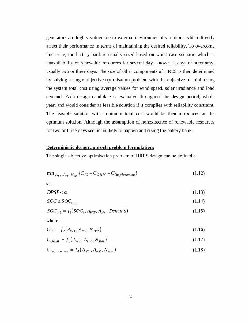
24
generators are highly vulnerable to external environmental variations which directly
affect their performance in terms of maintaining the desired reliability. To overcome
this issue, the battery bank is usually sized based on worst case scenario which is
unavailability of renewable resources for several days known as days of autonomy,
usually two or three days. The size of other components of HRES is then determined
by solving a single objective optimisation problem with the objective of minimising
the system total cost using average values for wind speed, solar irradiance and load
demand. Each design candidate is evaluated throughout the design period; whole
year; and would consider as feasible solution if it complies with reliability constraint.
The feasible solution with minimum total cost would be then introduced as the
optimum solution. Although the assumption of nonexistence of renewable resources
for two or three days seems unlikely to happen and sizing the battery bank.
Deterministic design approch problem formulation:
The single-objective optimisation problem of HRES design can be defined as:
}{min Re&,, placementMOICNAA CCCBatPVWT
(1.12)
s.t.
DPSP (1.13)
minSOCSOC (1.14)
DemandAASOCfSOC PVWTtt ,,,11 (1.15)
where
BatPVWTIC NAAfC ,,2 (1.16)
BatPVWTMO NAAfC ,,3& (1.17)
BatPVWTtreplacemen NAAfC ,,4 (1.18)

25
1.7.2 Stochastic design approach
In stochastic design approach, one or more than one design variables are involving
uncertainties, here the wind speed and solar irradiance as a result the power generated
by these resources are random values. Considering the uncertainties during the design
process can result in more reliable design output. However in this design method the
main challenge would be modelling the uncertainties in the most accurate way. The
first step in stochastic design approach is to find the best suited model for uncertain
variables
Modelling uncertainties:
Here two different approaches in modelling uncertainties are discussed.
a) Time series analysis, Auto Regressive Moving Average models
Time series analysis could be a viable method to model the uncertainties with
unknown variations. The special feature of time series analysis is the fact that
successive observations are not usually independent. Most time series are stochastic
and there would not be the possibility of exact prediction so the accuracy of future
values is conditioned by the knowledge of past values. Having sufficient historical
data on wind speed and solar radiation values in desired location, an Auto Regressive
Moving Average (ARMA) model can be fitted to the historical data of wind speed
and solar irradiance data to be used as the random generator in performance
evaluation of HRES design candidates.
The ARMA model is usually fitted to correlated time series data and is a way in
predicting the future value of time series. This model has two parts; autoregressive
(AR) and moving average (MA). The mathematical formulation of ARMA is:
qtqttptpttt ccyayayay ...... 112211 (1.19)

26
where p and q are ARMA model orders, paa ,...,1 are the autoregressive parameters,
qcc ,....1 are the moving average parameters and qtt ,..., are random variables with
mean value of zero and standard deviation of .
The ARMA model orders and parameters are estimated as follow:
Transformation of the historical data
Transformation of input data is performed if required in order to stabilize the variance
and make the data more normally distributed. To check the necessity the
transformation the skewness of the data set can be used as a measure of normality.
Skewness is a measure of asymmetry of the data around the sample mean and is
defined as the third standardised moment and is calculated as:
3
3)(
xEs (1.20)
where is the mean value of x , is the standard deviation of x , and )(tE represents
the expected value of quantity of t . The negative value of skewness means the data
are spread out more to the left of the mean and if the data are more spread out more to
the right of the mean the value of the skewness would be positive. The skewness of
the normal distribution is zero. There are various methods to transform the data set to
Gaussian form.
Power Transformation
Brown [66] introduced a method to transform the Weibull distribution into Gaussian
form as :
mttT UU )()( with nt ,...,2,1 (1.21)
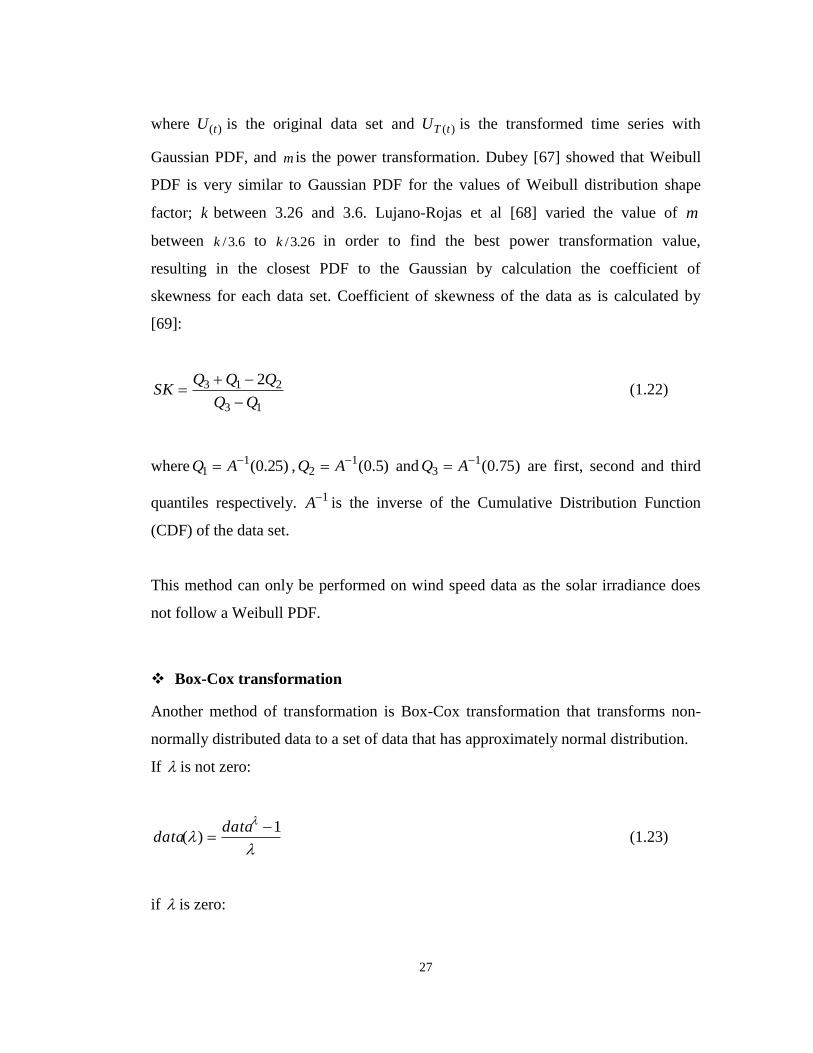
27
where )(tU is the original data set and )(tTU is the transformed time series with
Gaussian PDF, and m is the power transformation. Dubey [67] showed that Weibull
PDF is very similar to Gaussian PDF for the values of Weibull distribution shape
factor; k between 3.26 and 3.6. Lujano-Rojas et al [68] varied the value of m
between 6.3/k to 26.3/k in order to find the best power transformation value,
resulting in the closest PDF to the Gaussian by calculation the coefficient of
skewness for each data set. Coefficient of skewness of the data as is calculated by
[69]:
13
213 2
QQQSK
(1.22)
where )25.0(11
AQ , )5.0(12
AQ and )75.0(13
AQ are first, second and third
quantiles respectively. 1A is the inverse of the Cumulative Distribution Function
(CDF) of the data set.
This method can only be performed on wind speed data as the solar irradiance does
not follow a Weibull PDF.
Box-Cox transformation
Another method of transformation is Box-Cox transformation that transforms non-
normally distributed data to a set of data that has approximately normal distribution.
If is not zero:
1)(
datadata (1.23)
if is zero:
28
)log()( datadata (1.24)
To find the best form of transformation in this study, the results of performing Power
transformation and Box Cox transformation and the original data set of wind speed
are compared in terms of the value of skewness and the series with the closest value
to zero of skewness is chosen. For solar irradiance the result of Box cox
transformation is compared to the original data and the series with the absolute value
of skewness closer to zero is selected.
Dickey-Fuller test
To evaluate the stationarity of the data the Augmented Dickey Fuller test is used [70,
71]. This test checks whether a unit root is present in autoregressive model.
ttt yy 1 (1.25)
where ty is the variable of interest; is a coefficient and t is the error term. A unit
root is present if is 1. In case of the presence of unit root in the model the data
would be non-stationary and needs to transform to a stationary data set by performing
de-trending process. The non-stationary data can be transformed to stationary by.
Fitting a smooth curve to the existing trend.
Differentiate the curve until the remaining trend is negligible.
Order of ARMA model
The method for estimation of order of ARMA model was first introduced by Box
and Jerkins [72] which was based on judging the orders by visual appearance of
autocorrelation function (acf) and partial autocorrelation function (pacf) plots.
However, identifying the ARMA models orders by this method is very difficult and
requires a lot of experience even for simplest models.
29
Another method in ARMA model order identification is based on fitting a set of trial
candidate models and computing the goodness of fit of the models. The goodness of
fit of the models can be computed by Akaike Information Criterion (AIC) and Final
Prediction Error (FPE) [73]. The goodness of the fitted model is measured by
evaluation the models residuals.
N
nVAIC
21log (1.26)
Nn
Nn
VFPE
1
1 (1.27)
where V is the variance of model residuals N is the length of the time series and
qpn is the number of estimated parameters in ARMA model. The model with
lowest FPE and AIC value is then selected as the model of best fit.
Ljung-Box Test
If a good model is chosen and effectively describes the original data, it is expected
that the residuals to be random or uncorrelated because if the residuals are correlated
the prediction error would increase by time. Ljung-Box Test [74] is used to examine
the existence of correlation between the fitted ARMA model residuals[75]. If the
model is appropriate, then Q should be approximately distributed as 2 with
qpm degrees of freedom.
m
k
k
kN
rNNQ
1
2
)2( (1.28)

30
where N is the time series size, kr is the correlation if residuals at lag k . The null
hypothesis is rejected if Q is higher than chi-square distribution )(2 qpm .
Simulation and back-transformation
The data is simulated using fitted ARMA model and then back transformed to its
original scale [76].
Using this method an Auto Regressive Moving Average (ARMA) model is fitted to
the historical data of wind speed and solar irradiance data which can be used as the
random generator in performance evaluation of HRES design candidates.
The results obtained using this method is discussed in chapter 5.
b) Fitting the historical data to known distributions
One of common approaches is fitting the uncertainties to known distributions such as
Weibull or Beta distributions [77].
The performance of this method in modelling wind speed and solar irradiance are
compared to the output of performing time series analysis in chapter 6.
Stochastic design approch problem formulation:
Using either of discussed methods in modelling uncertainties in stochastic design of
HRES two approaches are followed in this work.
Stochastic design, approach 1 problem formulation
In this approach the wind speed and solar irradiance variations are modelled with
ARMA model. Using Monte-Carlo simulation the design candidates are evaluated in
terms of reliability and the optimum solution with minimum cost is obtained. The
optimisation problem is defined as:
31
}{ Re&,,
min placementMOICNAA
CCCimizeBatPVWT
(1.29)
s.t.
DPSPE (1.30)
minSOCSOC (1.31)
Demand,A,A,SOCfSOC PVWTt11t (1.32)
where
BatPVWTIC NAAfC ,,2 (1.33)
BatPVWTMO NAAfC ,,3& (1.34)
BatPVWTtreplacemen NAAfC ,,4 (1.35)
where DPSPE is the expected value of DPS .
The results obtained by using this method are discussed in chapter 5.
Stochastic design, approach 2 problem formulation
By replacing the expected value of the DPSP with the probability of deficiency in
generated power, the optimisation problem would change to an optimisation problem
with probabilistic constraint which can be solved by using chance-constrained
programming. Chance constrained programming is been used in various fields of
engineering where there is uncertainties involved.
In this approach the wind speed and solar irradiance variations are fit to known
distribution and chance constrained programming is used to obtain the optimum
solution. Here the generated power by wind turbine and PV panel are dependent
random variables following known distributions and the power of battery bank is
dependent random variable. Here the optimisation problem is defined as:
}{min Re&,, placementMOICNAA CCCBatPVWT
(1.36)
s.t.
32
)DemandPPr( tt (1.37)
tBattPVWTt PPPPt
(1.38)
minSOCSOC (1.39)
Demand,A,A,SOCfSOC PVWTt11t (1.40)
where
BatPVWT2IC N,A,AfC (1.41)
BatPVWT3M&O N,A,AfC (1.42)
BatPVWT4treplacemen N,A,AfC (1.43)
Chance constrained programming
Various optimisation problems in design and planning areas need to deal with
constraints involving random parameters, which are required to be satisfied within a
pre-defined probability. Mathematical formulation for designing reliability
constrained optimisation problems lead to chance constrained programming or
probabilistic programming. Chance Constrained Programming (CCP) was first
introduced by Charnes and Cooper [78] in 1959and later Miller and Wagner [79] and
Prekopa [80] introduced chance constrained programming for multivariate variables.
The main feature of CCP is that this method uses an effective way of modelling
uncertainty in optimisation problems in which the inequality constraints are satisfied
with a probability which is defined at the beginning of the process. The predefined
probability ensures a certain level of reliability [81]. Due to its high performance in
the solving the problems with high level of uncertainty, CCP is been widely used to
model reliability of technical and economic problems real time optimization [82]. The
general form of a chance constrained problem can be formulated as:
),(min xf (1.44)
s.t.
33
)0),(Pr( xG (1.45)
where ),( yf is the objective function which contains random variables,
y represents the vector of decision variables, represents the vector of k random
variables with given cumulative density functions that kjzzF jj,...,1),Pr()(
and krgr ,...,1, represents set of constraints involved with random variables. The
chance constrained method programming demands that the joint probability of k
individual constraints to be satisfied with a given probability level [83] of . There
might be some deterministic constraints in the problem which are shown with ip .
To solve the chance constrained problem if the ),( yg j can be expressed linearly in
the form of i
jijij kjyTyg ,....,1,),( it can be shown that each of
individual chance constraints can be re-written as:
ZVarEyT jjiji )()( (1.46)
)1
1(1
kZ
(1.47)
where ()E and ()Var are the expected value and variance of the random variable and
the standard normal cumulative density function is shown by () .
This method has been used for optimal sizing of HRES in the desired site and the
results are presented in chapter 6.
1.8 Scope of thesis and contribution to the knowledge
This thesis will focus on the different design approaches in optimal sizing of HRES.
Following a deterministic design approach:
an economic analysis on optimal sizing of a grid-connected HRES shows that
based on grid electricity price; considering a small storage, battery bank, to

34
supply the deficit of produced power in renewable resources may prove to be
more cost effective than conventional method of buying from grid.
it is shown that although the HRES components might be sized based on
worst case scenario, the system might not be able to perform satisfactory if
only the overall performance of the system is considered without a detailed
study on the time and period of blackout occurrence although its overall
reliability measure might meet the design constraint.
In order to maintain a high performance HRES which is cost effective, green, and
durable and with good output quality, instead of deterministic design approach which
is traditionally used in design of HRES, different stochastic design approaches are
proposed. The effect of uncertainties in the renewable resources during the design are
considered by
time series analysis which is performed on historical data of wind speed and
solar irradiance and fitted ARMA models to each hour of a typical day of
each month of the year is used to as the random data generator in Monte
Carlo simulation for a realistic design output.
through a case study it is shown that the choice of modelling method for the
wind speed and solar irradiance should be done by comparing the statistical
characteristic of different approaches; fitting an ARMA model to using the
known distributions; and it is completely dependent on the location of the
desired site.
through a comparison between common method of chance constrained
programming with the assumption of the random variables following a bi-
variant Gaussian distribution and the novel proposed method that solves the
chance constrained problem based on calculating the joint CDF of the
unknown joint distribution of the random variables, it is shown that the
common method is limiting the feasible region of solutions and results in a
more conservative and naturally less cost effective optimum solution.
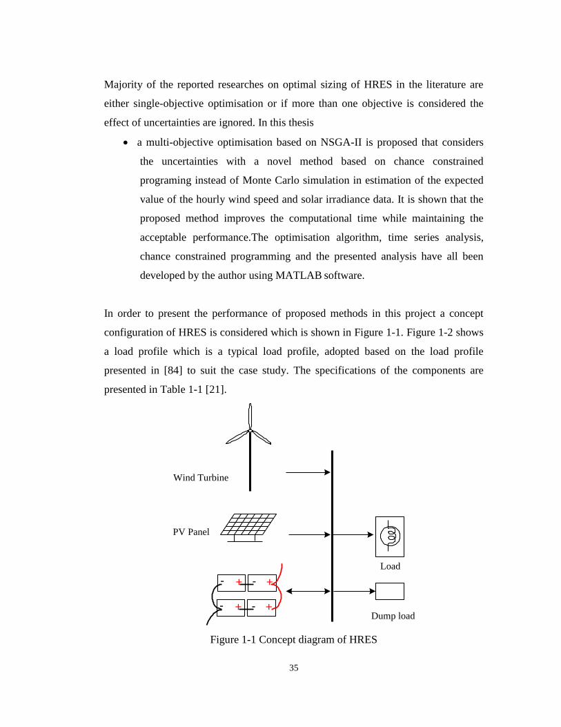
35
Majority of the reported researches on optimal sizing of HRES in the literature are
either single-objective optimisation or if more than one objective is considered the
effect of uncertainties are ignored. In this thesis
a multi-objective optimisation based on NSGA-II is proposed that considers
the uncertainties with a novel method based on chance constrained
programing instead of Monte Carlo simulation in estimation of the expected
value of the hourly wind speed and solar irradiance data. It is shown that the
proposed method improves the computational time while maintaining the
acceptable performance.The optimisation algorithm, time series analysis,
chance constrained programming and the presented analysis have all been
developed by the author using MATLAB software.
In order to present the performance of proposed methods in this project a concept
configuration of HRES is considered which is shown in Figure 1-1. Figure 1-2 shows
a load profile which is a typical load profile, adopted based on the load profile
presented in [84] to suit the case study. The specifications of the components are
presented in Table 1-1 [21].
PV Panel
Load
Wind Turbine
++ --
++ --Dump load
Figure 1-1 Concept diagram of HRES
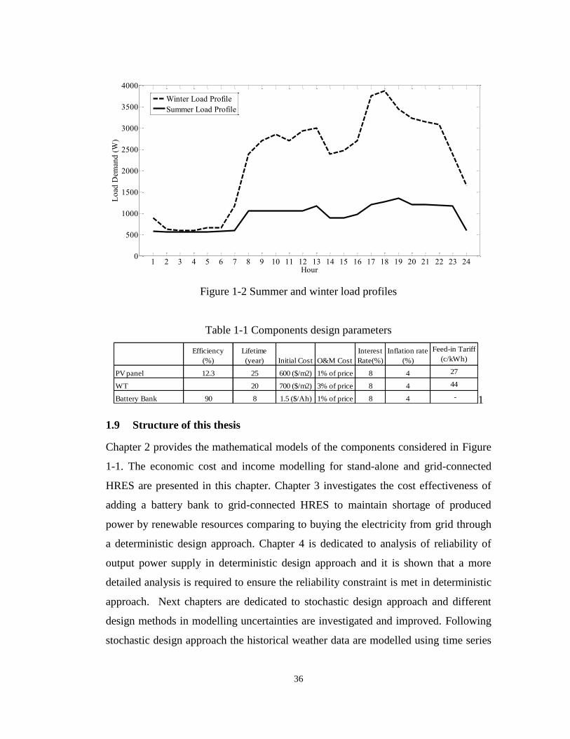
36
1 2 3 4 5 6 7 8 9 10 11 12 13 14 15 16 17 18 19 20 21 22 23 240
500
1000
1500
2000
2500
3000
3500
4000
Hour
Lo
ad D
eman
d (
W)
Winter Load Profile
Summer Load Profile
Figure 1-2 Summer and winter load profiles
Table 1-1 Components design parameters
Efficiency
(%)
Lifetime
(year) Initial Cost O&M Cost
Interest
Rate(%)
Inflation rate
(%)
Feed-in Tariff
(c/kWh)
PV panel 12.3 25 600 ($/m2) 1% of price 8 4 27
WT 20 700 ($/m2) 3% of price 8 4 44
Battery Bank 90 8 1.5 ($/Ah) 1% of price 8 4 - 1
1.9 Structure of this thesis
Chapter 2 provides the mathematical models of the components considered in Figure
1-1. The economic cost and income modelling for stand-alone and grid-connected
HRES are presented in this chapter. Chapter 3 investigates the cost effectiveness of
adding a battery bank to grid-connected HRES to maintain shortage of produced
power by renewable resources comparing to buying the electricity from grid through
a deterministic design approach. Chapter 4 is dedicated to analysis of reliability of
output power supply in deterministic design approach and it is shown that a more
detailed analysis is required to ensure the reliability constraint is met in deterministic
approach. Next chapters are dedicated to stochastic design approach and different
design methods in modelling uncertainties are investigated and improved. Following
stochastic design approach the historical weather data are modelled using time series

37
analysis and used to design a HRES for desired site. The methodology and results are
presented in Chapter 5. Chapter 6 compares the results of conventional approach in
solving chance constrained problems which is based on the assumption of
considering the Gaussian distribution to present the randomness of uncertain
variables with a proposed method which solves the chance constrained problem
considering the joint distribution of random variables as unknown. Chapter 7
performs a multi-objective optimisation based on NSGA-II with a novel method in
integrating the uncertainties in design based on chance constrained programming.
Chapter 8 concludes the thesis with several remarks of the finished project along with
future research directions.

38
2 Modelling
39
2.1 HRES components
The HRES design is crucially dependent on the performance of its individual
components. In order to analyse the overall system performance the individual
components need to be modelled first. Different mathematical models are proposed
by researchers to estimate the output power of wind turbine, photovoltaic panel and
batteries. The models implemented in this study are chosen with consideration of
giving a realistic estimation of the output of each system without being too
complicated with details.
2.1.1 Wind Turbines
Wind energy has been a popular alternative power source in recent years and many
researches have been done to demonstrate the potential of this renewable power
source around the world [85]. Although the power production from wind energy is
challenging due to its dependency to weather conditions studies show that wind is a
periodical phenomenon for large geographical areas [86]. However wind energy may
not be available everywhere because of low wind speed, it can be an attractive and
economically viable energy resource in many locations around the world. A wind
turbine converts available power in the wind into electricity. The capacity of wind
turbines varies from a few watts which can be used in residential and commercial
application to Megawatts in wind plants. Nowadays, wind turbines are categorized to
horizontal-axis wind turbines (HAWT) and vertical-axis wind turbines (VAWT). The
shaft and electrical generator are located on top of the tower of HAWT and the
turbine is pointed to the wind direction, where the main rotor of the VAWT is set
vertically and is not pointed to the wind. Although the VAWT have a simple
installation and control, since they cannot produce as much power of HAWT, they are
not as favourable as HAWT so the majority of installed HAWTs today are from the
HAWT type. Figure 2-1 presents a two configuration of wind turbine.
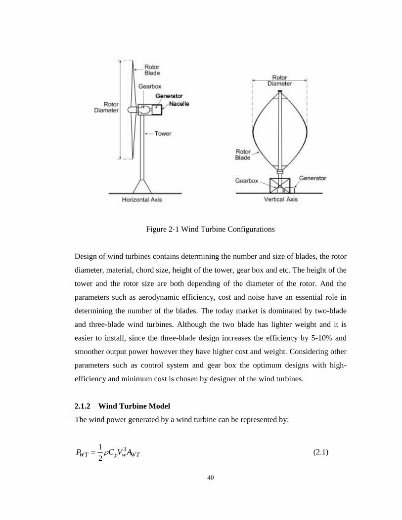
40
Figure 2-1 Wind Turbine Configurations
Design of wind turbines contains determining the number and size of blades, the rotor
diameter, material, chord size, height of the tower, gear box and etc. The height of the
tower and the rotor size are both depending of the diameter of the rotor. And the
parameters such as aerodynamic efficiency, cost and noise have an essential role in
determining the number of the blades. The today market is dominated by two-blade
and three-blade wind turbines. Although the two blade has lighter weight and it is
easier to install, since the three-blade design increases the efficiency by 5-10% and
smoother output power however they have higher cost and weight. Considering other
parameters such as control system and gear box the optimum designs with high-
efficiency and minimum cost is chosen by designer of the wind turbines.
2.1.2 Wind Turbine Model
The wind power generated by a wind turbine can be represented by:
WTwpWT AVCP 3
2
1 (2.1)
41
where WTP is the wind turbine output power in W , 3/225.1 mkg is the air
density, pC is the wind turbine power coefficient, WTA is the rotor disk area in 2m
and wV is the hourly average wind velocity in sm at the hub elevation.
The wind speed varies with the height and the wind data measurement equipment is
installed at different heights so it is crucial to calculate the wind speed at the wind
turbine hub. The wind speed wV at the hub height can be calculated as:
0
0
ln
ln
z
z
zz
VVref
hub
refw (2.2)
where hubz is the hub height; refV is the wind speed at the reference height refz and
0z is the surface roughness length in m . Wind speed at any given height of the tower
can be found if the surface roughness and wind measurements at different height are
available. The value of 0z in logarithmic law for open farm is assumed as 0.03.
The power coefficient depends on the wind turbine characteristics and varies with the
wind speed. In this study, the power curve of the different wind turbines are used to
calculate the corresponding Cp value to different wind speeds. Using the least square
method a mathematical model is fitted to the points to model the PC value variation
at different wind speeds as:
11
21 qq
qqP CvCvCvCC (2.3)
42
A least-square problem is a category of optimisation problem which does not include
constraints. The objective of this optimisation problem is to minimise the sums of
squares of the form iTi bxa [87]. The optimisation problem can be written as
21 )()(min i
ki
Ti bxaxf (2.4)
where nkA , Tia are the rows of A and the vectors nx is the optimisation
variables. The optimisation problem 2.4 can be solved by solving a set of linear
equations.
bAxAA TT )( (2.5)
And from 2.5 we would have
bAAAx TT 1)( (2.6)
Using least square curve fitting to extract the best fitted curve to the observed Cp vs.
wv for the WTn observed wind turbines and vn wind speeds that the Cp values are
known the elements of for a polynomial of the order of q Equation 2.6 can be written
as:
1)1( qCx (2.7)

43
)1()1(
0
0
)1(
011
011
qnnqn
n
q
n
n
q
n
qn
q
q
WTvWT
vv
vv
WT
vv
vv
vv
vv
A
(2.8)
11
1
,
,1
1,
1,1
vWTWT
vnWTn
vn
WTWTn
nnn
P
P
nP
P
c
c
c
c
B
(2.9)
Using the curve fitting tool in MATLAB software a polynomial is fitted to extract a
generic Cp equation to be used in the calculations.
Following described method on the data of different wind turbines in the range of
kW1 to kW15 ; Figure 2-2; applied to the case study used in this project the PC
variation is modelled by:
0.001027- 0.11-0.07874
0.01295- 0.9088 2.95e- 3.646e
2
34-35-56-7
ww
wwwwp
vv
vvevvC
(2.10)
2.1.3 Photovoltaic Panels
Solar energy is one of the most significant energy resources available to be used in
producing the increasing power demand of the world. Solar energy can be used in
solar thermal systems which convert the solar energy into required thermal energy

44
0 2 4 6 8 10 12 14 16 18 20 22 24
0.1
0.2
0.3
0.4
0.5
Wind Speed (m/s)
Cp
1kW
2.5kW
3kW
5kW
6kW
9kW
10kW
11kW
13kW
15kW
Fitted Curve
Figure 2-2 Cp curves of different wind turbines in the range of kW1 to kW15
form or they can be used in photovoltaic systems that convert the solar energy to
electricity. Among these two main uses of solar energy, converting to electricity is the
interest of this study. The efficiency of the photovoltaic panels has improved
significantly from 4% for first model which was developed in 1954 by Chaplin,
Fuller and Pearson to over 40% recently [88].
The semiconductors in structure of photovoltaic panels produce electricity by
absorbing the solar irradiation coming through them. Solar cells consist of large-area
semiconductor diode [89]. The p-n junction is created by adding impurity to the
semiconductor crystal. Since there are four electrons required to fit an atom to the
crystal structure if the impurities are phosphorus-atoms with five outer electrons, four
would be used to fit to the crystal structure and one would remain free. In this case
there would be a region with majority of free negative charge which is called n-
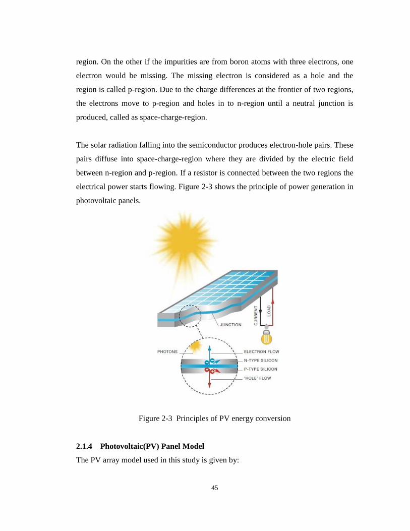
45
region. On the other if the impurities are from boron atoms with three electrons, one
electron would be missing. The missing electron is considered as a hole and the
region is called p-region. Due to the charge differences at the frontier of two regions,
the electrons move to p-region and holes in to n-region until a neutral junction is
produced, called as space-charge-region.
The solar radiation falling into the semiconductor produces electron-hole pairs. These
pairs diffuse into space-charge-region where they are divided by the electric field
between n-region and p-region. If a resistor is connected between the two regions the
electrical power starts flowing. Figure 2-3 shows the principle of power generation in
photovoltaic panels.
Figure 2-3 Principles of PV energy conversion
2.1.4 Photovoltaic(PV) Panel Model
The PV array model used in this study is given by:
46
PVPVPV IAP (2.11)
where PVP is the PV array output power inW , I is the horizontal solar irradiance in
2/ mW , PVA is the PV panel area in 2m and PV is the efficiency of the PV array and
is calculated as [11]. Although the total solar irradiation of depends on position of the
sun that varies from month to month, instead of estimating the amount of total solar
radiation with the deterministic method which use the direct normal and diffuse solar
radiations, in this study the historical data which is actually measured is used in
stochastic approaches to implement the factor of uncertainty in estimating the solar
power in the desired site.
The effect of the temperature on the efficiency of the PV panel is considered using:
)(1 rcrPV TT (2.12)
where r is the module reference efficiency, is the array efficiency temperature
coefficient, rT is the reference temperature for the cell efficiency and cT is the
monthly average cell temperature [90] and can be calculated as follows:
IU
TTL
ac
(2.13)
where aT is the instantaneous ambient temperature,
)( ,
,
NOCTa
NOCTT
LTNOCT
I
U
(2.14)

47
NOCT is normal operating cell temperature, CT NOCTa 20, and
2, /800 mWI NOCTT , for a wind speed of sm /1 .
2.1.5 Storage System
Energy storage system has an important role in maintaining energy balance in HRES
production and load demand. As it enables the system to store the excessed energy
when the production is high and demand is low for example during the day and use it
at times when there is deficit of supply. Different type of energy storages can be used
in HRES such as Compressed Air Energy Storage, Hydrogen Fuel cells and Batteries.
Among them batteries are more popular in HRES as they do not enquire any auxiliary
systems to be run in conjunction to them and they offer best technology for required
reliability and efficiency and cost in HRES.
Batteries are available in variety of types such as Lithium Ion (LiIon), Sodium
Sulphor (NaS), Nickel Cadmium (NiCd) and Lead Acid batteries. LiIon batteries
have the characteristic of high efficiency and lifespan at high depths of discharge
however they are currently too expensive. NaS batteries have temperature constraint
for their optimal use and NiCd batteries have high rate of self-discharge which make
them less ideal for use in HRES. So far Lead Acid batteries have been the most
popular type of storage in HRES [91, 92].
2.1.6 Battery bank Model
Common drawback of using renewable resources is their unpredictable nature which
is completely dependent on weather conditions and may result in load rejection at
some points. In standalone HRES, the balance between demand and generation is
obtained by an auxiliary power source such as a diesel generator or a battery bank.
The battery used in this study is a lead acid battery. The selection of an appropriate
size of a battery bank requires complete analysis on the charge and discharge process
of the battery which depends on the load profile and the output of wind turbine and
48
PV panels. The property of the battery related to the performance of HRES is the
state of charge ( SOC ) of the battery at each analysis time step. SOC is simulated
during the charging process as [93]:
Bat
CtBat
tt1tc
ΔtI )δ(1SOCSOC
(2.15)
where, )(t is the hourly self-discharge rate (an average value of 0.02% is used in this
study). t is the time step for calculating the SOC (in this study, t is equal to one
hour). Batc is the nominal battery bank capacity in Ahand C is the charge efficiency
factor. The battery current BatI can be calculated as:
Bat
tloadtWTtPV
tBatV
PPPI
(2.16)
where, BatV is the battery voltage.
During the discharge, SOC is calculated as [93]:
Bat
tBattt
c
tISOCSOC
)1( t1 (2.17)
in which
V
PPPI tWTtPVtload
tBat
(2.18)
Charge and discharge processes are subjected to the following constraints:
maxmin 1 DODSOC (2.19)
49
where maxDOD is the maximum depth of discharge of the battery.
maxmin SOCSOCSOC t (2.20)
and
t
cSOCtSOC
tSOCSOCcCI
tIbat
bat )1)()((
))(((,
min,0max)(min
maxmax
max, (2.21)
The constant c is considered 1 if battery is charging and 0 if the battery is
discharging.
2.1.7 Battery lifetime
Lifetime of the battery is limited by two independent factors, the battery’s float and
the life battery’s cycle life. The battery’s float life is the maximum duration that the
battery will last before being replaced even if it has not been used at all. Dispatch
strategy has direct effect on battery’s lifetime, and by each charge and discharge
cycle some depletion happens in battery. Ashari et al. [26] used equivalent full cycles
(EFC) for measuring battery’s lifetime taking in to account the depth of discharge in
each charge and discharge cycle.
DODcyclesofNoEFC DOD__ (2.22)
where EFC is the Equivalent Full Cycles, DOD is Depth of Discharge and
DODcyclesofNo __ is number of charge–discharge cycles at the given DOD .
An average avEFC is calculated and after all the equivalent cycles the battery needs to
be replaced.
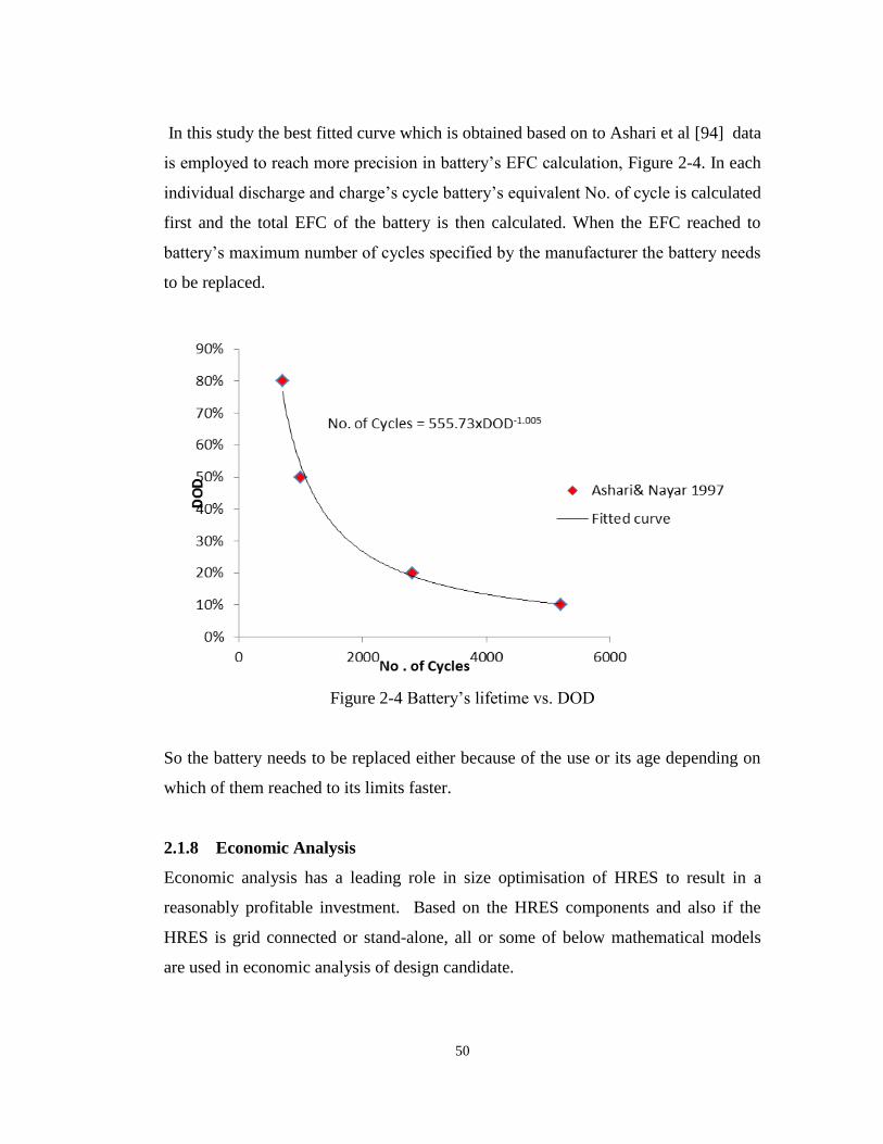
50
In this study the best fitted curve which is obtained based on to Ashari et al [94] data
is employed to reach more precision in battery’s EFC calculation, Figure 2-4. In each
individual discharge and charge’s cycle battery’s equivalent No. of cycle is calculated
first and the total EFC of the battery is then calculated. When the EFC reached to
battery’s maximum number of cycles specified by the manufacturer the battery needs
to be replaced.
Figure 2-4 Battery’s lifetime vs. DOD
So the battery needs to be replaced either because of the use or its age depending on
which of them reached to its limits faster.
2.1.8 Economic Analysis
Economic analysis has a leading role in size optimisation of HRES to result in a
reasonably profitable investment. Based on the HRES components and also if the
HRES is grid connected or stand-alone, all or some of below mathematical models
are used in economic analysis of design candidate.

51
2.1.9 Income Modelling
a) Income of feed-in tariff
In some countries based on the amount of the power HRES generates and used
domestically, the owner receives some income, called as feed-in tariff which is
calculated with:
)( ,, loadPVPVloadWTWTPFIT PFITPFITLI (2.23)
where WTFIT and PVFIT are feed-in tariff of wind turbine and PV panels respectively
. loadWTP , and loadPVP , are the wind turbine and PV panels’ production which is used
domestically.
b) Income of selling to grid
In case that the HRES is connected to the grid and there is the capacity in the grid to
buy the electricity from micro girds, the excess of generated power can be sold to the
grid and the income can be calculated by:
)( ,,,, excessPVexcessWTtgridsellPgridSellPPTLI
(2.24)
where gridsellT , is tariff of selling unit power to the grid. excessWTP , and excessPVP , are
excess power of wind turbine and PV panel which are calculated after load
satisfaction and charging the battery (if existed).
2.1.10 Cost Modelling
Economic analysis is an important factor to consider in size optimisation of HRES in
order to achieve a reasonably profitable investment. In this study the total cost of the
system TC (of the design candidates) is calculated as the economical measure taking
52
into account the initial capital cost ( ICC ), replacement cost ( treplacemenC ) and
present value of maintenance cost ( MOC & ). That is:
MOtreplacemenIC CCCTC & (2.25)
a) Initial Capital Cost
The initial capital cost consists of the cost of components and their installation cost.
0,,, )( CCcNCACAC BatUnitBatBatWTUnitWTPVUnitPVIC (2.26)
PVA and PVUnitC , are the total PV Area 2m and unit cost 2/$ m of the PV array,
respectively. WTA and WTUnitC , are the total rotor disk area and unit cost of the wind
turbine, respectively. BatN , Batc and BatUnitC , are the total number, nominal capacity
Ah and the unit cost Ah/$ of the battery bank, respectively. 0C is the total
installation constant cost including the cost of installation of the wind turbine and PV
panels and is considered to be 20% of the component cost of the wind turbine and
40% of the component cost of the PV system [21].
b) The Present Value of Replacement Cost
In this study the only component which needs to be replaced during life time of the
HRES is assumed to be the battery bank so this cost is only calculated when the
battery bank exists in the configuration.
The replacement cost of the battery bank can be calculated as [21]:
53
rep rep
iN
i
NN
dBatBattreplacemen
k
fCcNC
1
1
BatUnit,1
1 (2.27)
where BatN , Batc and BatUnitC , are the total number, nominal capacity and the unit
cost of the battery bank, respectively.
repN is the number of replacements over the system life span, f inflation rate; dk
annual real interest rate. The value of repN is calculated based on the number of
charge and discharge cycles; EFC .
c) The Present Value of Operation and maintenance Cost
The present value of operation and maintenance cost of the hybrid system is
expressed as[21]:
,
,1
11)
1(
0
0
)&(
)&(
,&
YC
k
f
fk
fC
C
MO
Y
ddMO
HRESMO
fk
fk
d
d
(2.28)
where Y is the system life span in years, 0)&( MOC is the operation and maintenance
cost in the first year.
0)&( MOC can be given as a fraction ( k ) of the initial capital cost ICC as:
ICMO kCC 0)&( (2.29)
The value of k is assumed to be 1% for the PV system, 3% for wind turbine and 1%
for battery bank [21].

54
d) The present value of buying electricity from grid
In grid-connected HRES, grid can provide the shortage of the power to satisfy the
demand the cost of maintaining the power shortage from grid can be calculated by:
)(
) (
,,
,,,,,
offpeakshortagegridoffpeakp
peakshortagegridpeakoffpeakshortagegridoffpeakpgridbuy PLCEL
PLCEPLCELC
)(
)(
b
a
(2.30)
pL system life period in years
)(a if there is no battery bank
)(b when there is battery bank
55
3 Optimal sizing of grid-
connected hybrid wind-
PV systems with battery
bank
56
3.1 Introduction
Conventionally a battery bank is used as the backup system in standalone Hybrid
Renewable Energy Systems (HRES) while in grid-connected systems the grid
performs as the backup during power shortage periods. For the latter, different prices
of electricity during peak and off-peak hours raises a question about the cost
effectiveness of using the grid as a backup. Adding a small storage system to
maintain the shortage of electricity produced by renewable resources at peak hours
may prove to be more cost effective backup. This chapter focuses on the design of an
optimised grid connected small-scale HRES, incorporating a battery bank to store
electricity during off-peak periods and uses this storage to support the HRES during
peak demands. This system is intended to be cost effective (taking into consideration
the Feed-In-Tariff) and make building self-sufficient with regard to energy use.
The performance of the proposed design method is evaluated based on a case study
for a typical household in UK.
Increase in energy demand has made the renewable resources more attractive.
Common drawback of using renewable resources is constant challenge with their
unpredictable nature which is completely dependent on climate changes and may
result in load rejection at some points. Conventionally the balance between demand
and HRES is obtained by grid in grid-connected systems and overproduction is sent
into the grid. In these systems, the grid performs as the storage system with infinite
capacity which makes the HRES reliable at any time. However different grid
electricity prices in peak and off-peak hours could become an economical challenge
in maintaining power shortage in peak hours from the grid. In this chapter a new
method in design of HRES is introduced by adding a small battery storage system to
cover the power shortage during peak hours.
Normally battery bank is used as a backup in standalone systems. Bernal-Agustín and
Dufo-López [48, 49] put their effort in analysing the main strategies in optimisation
of hybrid systems with battery bank as storage. Balamurugan et al. [19] proposed a
57
hybrid energy system consisting of biomass, wind, solar photovoltaic and battery to
deliver energy at optimum availability, considering proper energy storage to meet the
peak load demand during low or no solar radiation periods or during low wind
periods. Ould Bilal et al. [41] & Yang [93] & Kaabeche [21] proposed methods for
sizing a hybrid solar–wind-battery system with the aim of minimising cost system
with maximum reliability.
Recently some research has been carried out in which the hybrid system is grid-
connected but still includes a battery bank as storage. Castillo-Cagigal et al [95]
developed a prototype of a self-sufficient solar house equipped with grid connection,
PV generation, lead–acid batteries, controllable appliances and smart metering.
Mudler [96] proposed a method to determine the optimal storage size for grid-
connected dwelling with PV panels. Particularly increase in grid electricity prices for
example in peak hours will change the status of complete dependency on grid during
shortage times.
The presented study addresses the optimisation of a grid-connected HRES based on
wind and solar energy considering different grid electricity prices with a storage
system to cover the power shortages during peak hours.
3.2 Economic analysis
Economic analysis has a leading role in size optimisation of HRES to result in a
reasonably profitable investment. In this study the Return On Investment (ROI) of
the design candidates is calculated as the economical measure which is calculated
using:
100
TC
TCTIROI (3.1)
58
TI , the total income of the system takes into account the present value of feed-in tariff
income FITI and present value of selling excess electricity to the grid gridSellI , .
gridSellFIT IITI,
(3.2)
TC , the total cost of the system takes into account the initial capital cost ICC , the
present value of replacement cost repC and present value of maintenance
cost MOC & and present value of buying electricity from grid gridbuyC , .
gridbuyMOrepIC CCCCTC ,& (3.3)
3.3 Problem formulation & design scenarios
The objective is to find the optimum configuration of a grid-connected HRES with
maximum ROI while satisfying the load demand. The optimisation problem can be
formulated as:
100max
TC
TCTIROI
(3.4)
In this chapter the wind turbine/PV system sizing optimisation is performed
following a deterministic design approach. The averages hourly of weather data and
load profile are used as inputs of the design. The power from each resource is
calculated at each time step (every hour) based on the capacity of power generator.
The overall performance of each design candidate configuration is simulated during
the entire year.
In sizing of HRES components, two design scenarios are followed.

59
Scenario 1: Considering grid as the backup system in peak and off-peak hours and
selling excess of produced electricity to the grid. The total power of HRES is
calculated with below equation:
gridPVWT
PVWTHRESTotal PPP
PPP ,
)(
)(
b
a (3.5)
)(a if total power generated by wind turbine and PV is sufficient to cover the load
demand.
)(b if WTP and PVP is not sufficient to cover the load demand.
Scenario 2: Considering grid as the backup system in off-peak hours and battery bank
for peak hours.
The flow of excess power in this scenario is toward the battery bank if the battery is
not fully charged and in case that the battery is fully charged then the excess will be
sent to the grid.
To size the battery bank the amounts of excess energy and the peak hour power
shortage of each individual day is calculated and based on that data the battery bank
is sized. The battery is sized based on the worst day data using Equation 3.6.
BatBat
shortageBat
CDODV
tPN
max
(3.6)
where Load is maximum daily load )(Wh ; DS is the number of autonomy or storage
days in this study considered as 3days; BatV is the battery bank voltage in )(V ;
maxDOD is the maximum depth of discharge and Bat is the battery efficiency.
The performance of whole system is then simulated with equation:

60
Bat
gridPVWT
PVWT
HRESTotal
P
PPP
PP
P
,
_
)(
)(
)(
c
b
a
(3.7)
)(a if total power generated by wind turbine and PV is
sufficient to cover the load demand otherwise
)(b where WTP and PVP is not sufficient during off-peak hours
)(c where WTP and PVP is not sufficient during peak
hours and state of charge the battery :
minSOCSOC (3.8)
Feasible solutions of scenario 2 are compared with scenario 1 solutions and the most
satisfactory solution is then selected.
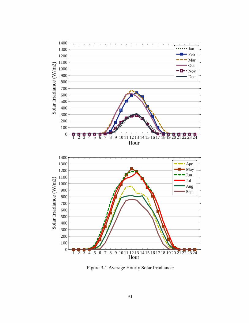
61
1 2 3 4 5 6 7 8 9 10 11 12 13 14 15 16 17 18 19 20 21 22 23 240
100
200
300
400
500
600
700
800
900
1000
1100
1200
1300
1400
Hour
So
lar
Irra
dia
nce
(W
/m2
)
Jan
Feb
Mar
Oct
Nov
Dec
1 2 3 4 5 6 7 8 9 10 11 12 13 14 15 16 17 18 19 20 21 22 23 240
100
200
300
400
500
600
700
800
900
1000
1100
1200
1300
1400
Hour
Sola
r Ir
radia
nce
(W
/m2)
Apr
May
Jun
Jul
Aug
Sep
Figure 3-1 Average Hourly Solar Irradiance:
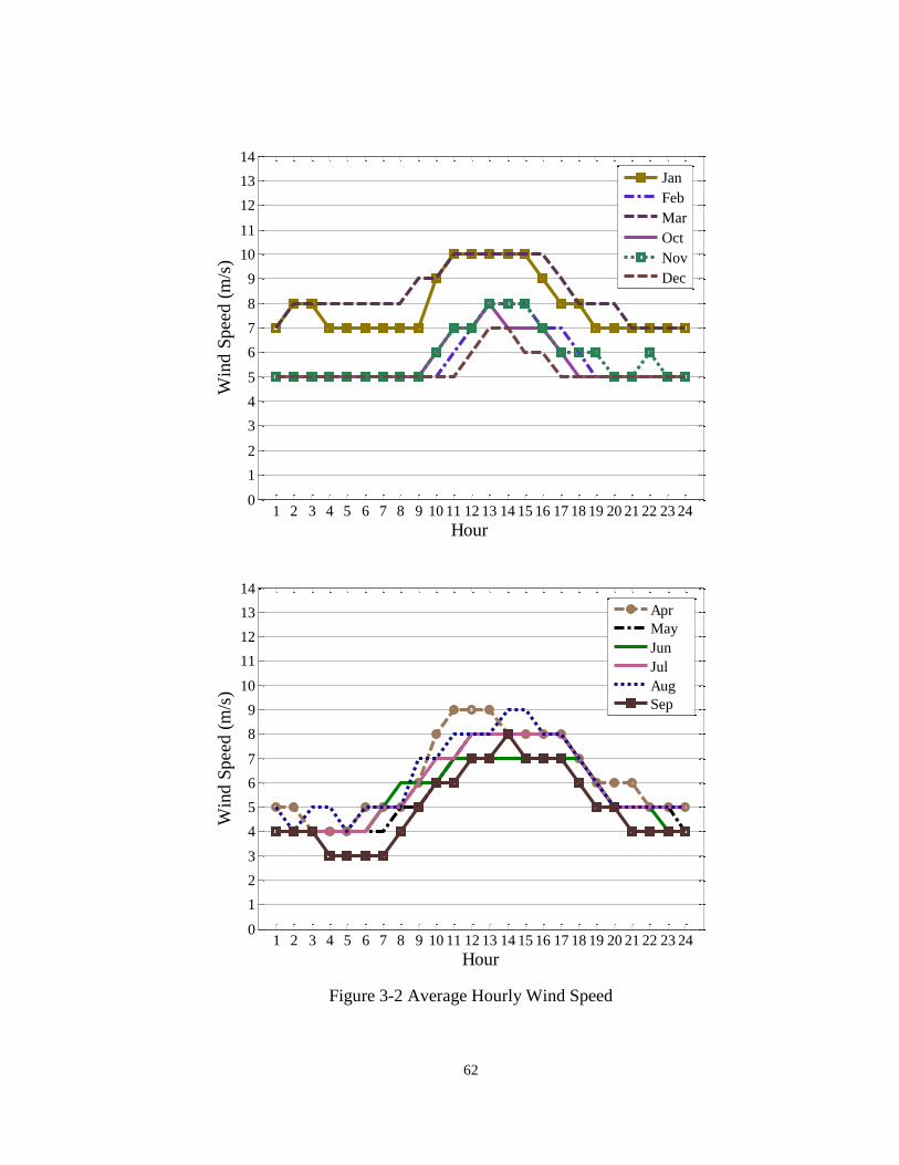
62
1 2 3 4 5 6 7 8 9 10 11 12 13 14 15 16 17 18 19 20 21 22 23 240
1
2
3
4
5
6
7
8
9
10
11
12
13
14
Hour
Win
d S
peed
(m
/s)
Jan
Feb
Mar
Oct
Nov
Dec
1 2 3 4 5 6 7 8 9 10 11 12 13 14 15 16 17 18 19 20 21 22 23 240
1
2
3
4
5
6
7
8
9
10
11
12
13
14
Hour
Win
d S
pee
d (
m/s
)
Apr
May
Jun
Jul
Aug
Sep
Figure 3-2 Average Hourly Wind Speed

63
3.4 Case study
The proposed methodology is used to design a grid-connected HRES for a household
in Kent; UK. Inputs of the design are typical summer and winter load profiles
presented in Figure 1-2 and hourly average of wind speed and solar irradiance data
for 12 months of the year which are presented in Figure 3-1 and Figure 3-2.
Technical and economical characteristics of the system components and grid prices
are given in Table 1-1 & Table 3-2.
As can be seen in Table 3-2 , the grid electricity has similar price during peak and
off-peak hours in the UK [97]. Therefore in this study the system is designed under
different assumptions for the peak hour’s price. Comparing the results comparison the
peak hour rate at which adding a storage system to cover the power shortage would
be more cost effective than buying the required electricity from grid will be obtained.
Table 3-1 The battery bank specification
Nomial Capacity
(Ah)
Nominal Voltage
(V)
DOD
(%)
Number of
Cycles
Battery
Bank40 24 90 535
Table 3-2 Grid electricity process in UK
GridOff-peak price
(c/kWh)
Peak price
(c/kWh)
First 900kWh 29 NA
Consumptions after
first 900kWh17 NA
Selling electricity to
grid (c/kWh)5 5
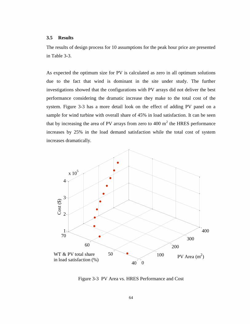
64
3.5 Results
The results of design process for 10 assumptions for the peak hour price are presented
in Table 3-3.
As expected the optimum size for PV is calculated as zero in all optimum solutions
due to the fact that wind is dominant in the site under study. The further
investigations showed that the configurations with PV arrays did not deliver the best
performance considering the dramatic increase they make to the total cost of the
system. Figure 3-3 has a more detail look on the effect of adding PV panel on a
sample for wind turbine with overall share of 45% in load satisfaction. It can be seen
that by increasing the area of PV arrays from zero to 400 m2 the HRES performance
increases by 25% in the load demand satisfaction while the total cost of system
increases dramatically.
0
100
200
300
400
40
50
60
701
2
3
4
x 105
PV Area (m2)
Cost
($)
WT & PV total share in load satisfaction (%)
Figure 3-3 PV Area vs. HRES Performance and Cost
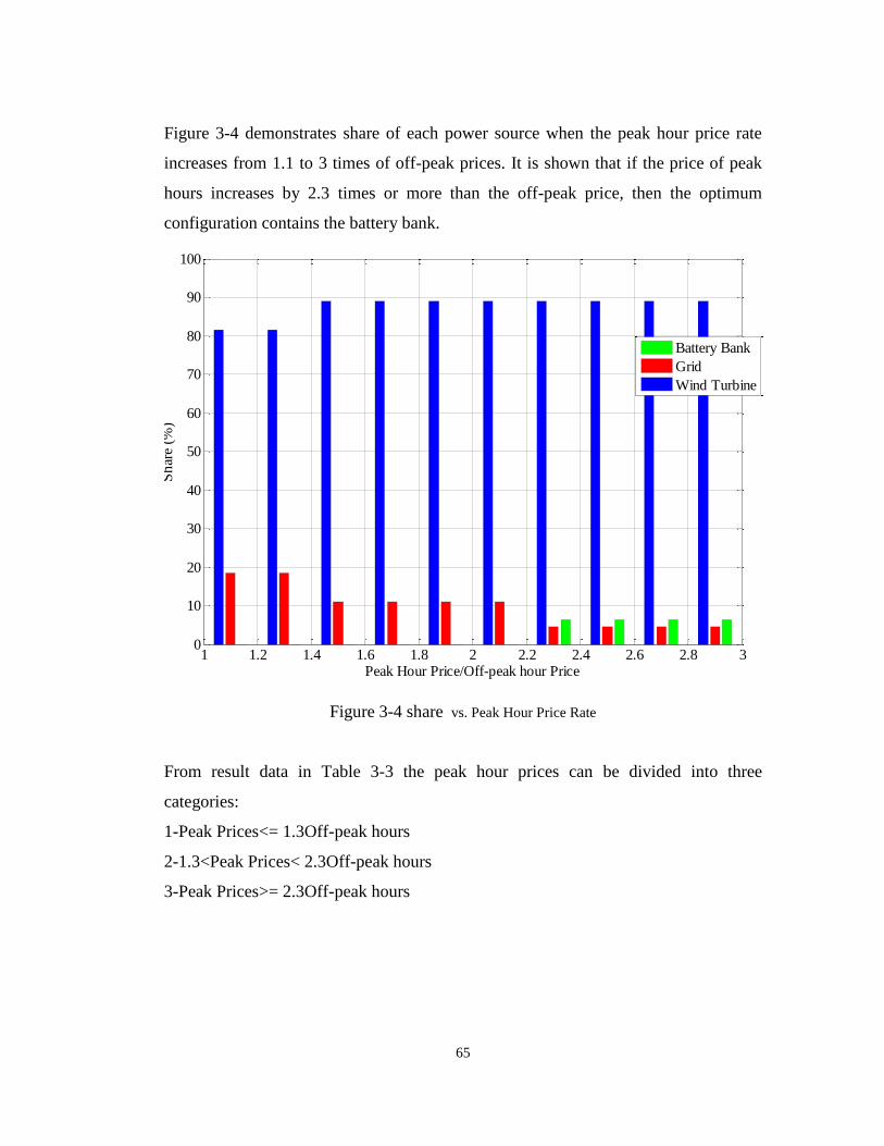
65
Figure 3-4 demonstrates share of each power source when the peak hour price rate
increases from 1.1 to 3 times of off-peak prices. It is shown that if the price of peak
hours increases by 2.3 times or more than the off-peak price, then the optimum
configuration contains the battery bank.
1 1.2 1.4 1.6 1.8 2 2.2 2.4 2.6 2.8 30
10
20
30
40
50
60
70
80
90
100
Peak Hour Price/Off-peak hour Price
Sh
are
(%)
Battery Bank
Grid
Wind Turbine
Figure 3-4 share vs. Peak Hour Price Rate
From result data in Table 3-3 the peak hour prices can be divided into three
categories:
1-Peak Prices<= 1.3Off-peak hours
2-1.3<Peak Prices< 2.3Off-peak hours
3-Peak Prices>= 2.3Off-peak hours
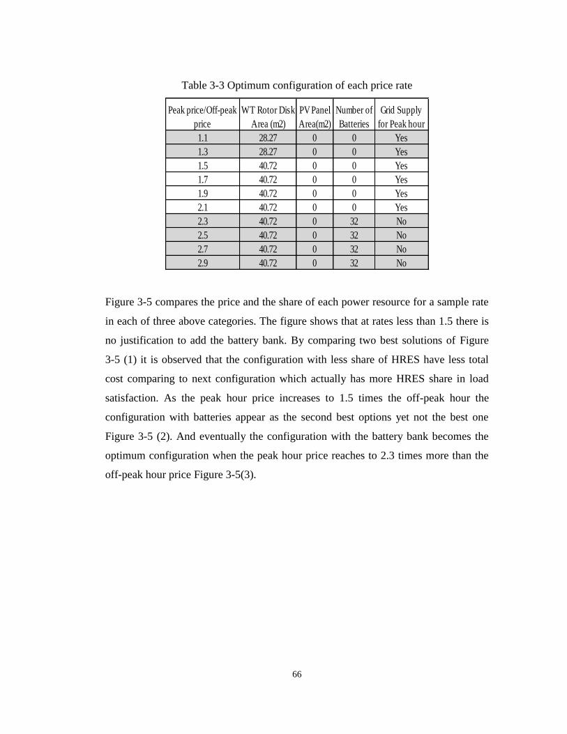
66
Table 3-3 Optimum configuration of each price rate
Peak price/Off-peak
price
WT Rotor Disk
Area (m2)
PV Panel
Area(m2)
Number of
Batteries
Grid Supply
for Peak hour
1.1 28.27 0 0 Yes
1.3 28.27 0 0 Yes
1.5 40.72 0 0 Yes
1.7 40.72 0 0 Yes
1.9 40.72 0 0 Yes
2.1 40.72 0 0 Yes
2.3 40.72 0 32 No
2.5 40.72 0 32 No
2.7 40.72 0 32 No
2.9 40.72 0 32 No
Figure 3-5 compares the price and the share of each power resource for a sample rate
in each of three above categories. The figure shows that at rates less than 1.5 there is
no justification to add the battery bank. By comparing two best solutions of Figure
3-5 (1) it is observed that the configuration with less share of HRES have less total
cost comparing to next configuration which actually has more HRES share in load
satisfaction. As the peak hour price increases to 1.5 times the off-peak hour the
configuration with batteries appear as the second best options yet not the best one
Figure 3-5 (2). And eventually the configuration with the battery bank becomes the
optimum configuration when the peak hour price reaches to 2.3 times more than the
off-peak hour price Figure 3-5(3).

67
5 5.25 5.5 5.75 6 6.25 6.5 6.75 7 7.25 7.5
x 104
0
10
20
30
40
50
60
70
80
90
100
Share
(%
)
Total Cost ($)
5 5.25 5.5 5.75 6 6.25 6.5 6.75 7 7.25 7.5
x 104
0
10
20
30
40
50
60
70
80
90
100
Retu
rn o
n I
nvestm
ent
(%)
Battery Share
Grid Share
Renewable Share
ROI
(1) Peak price=1.1 Off-peak
6.85 6.9 6.95 7 7.05 7.1 7.15 7.2 7.25
x 104
0
10
20
30
40
50
60
70
80
90
100
Share
(%
)
Total Cost ($)
6.85 6.9 6.95 7 7.05 7.1 7.15 7.2 7.25
x 104
0
10
20
30
40
50
60
70
80
90
100
Retu
rn o
n I
nvestm
ent
(%)
Battery Share
Grid Share
Renewable Share
ROI
(2) Peak price=1.9 Off-peak
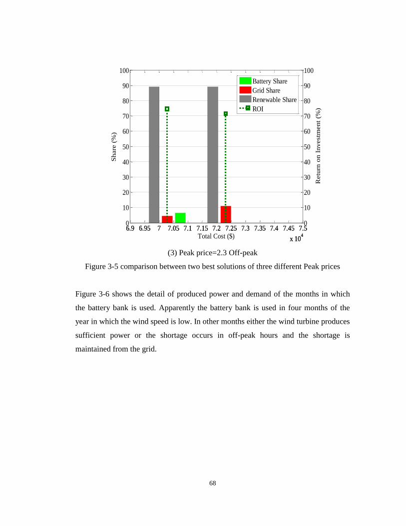
68
6.9 6.95 7 7.05 7.1 7.15 7.2 7.25 7.3 7.35 7.4 7.45 7.5
x 104
0
10
20
30
40
50
60
70
80
90
100
Sh
are
(%
)
Total Cost ($)
6.9 6.95 7 7.05 7.1 7.15 7.2 7.25 7.3 7.35 7.4 7.45 7.5
x 104
0
10
20
30
40
50
60
70
80
90
100
Retu
rn o
n I
nv
estm
en
t (%
)
Battery Share
Grid Share
Renewable Share
ROI
(3) Peak price=2.3 Off-peak
Figure 3-5 comparison between two best solutions of three different Peak prices
Figure 3-6 shows the detail of produced power and demand of the months in which
the battery bank is used. Apparently the battery bank is used in four months of the
year in which the wind speed is low. In other months either the wind turbine produces
sufficient power or the shortage occurs in off-peak hours and the shortage is
maintained from the grid.
69
Hour (February)
Pow
er (
W)
0 1 2 3 4 5 6 7 8 9 10 11 1213 14 15 16 17 18 19 20 21 22 23 240
500
1000
1500
2000
2500
3000
3500
4000
Demand
WT Power
Battery Power
Grid Power
Hour (October)
Pow
er (
W)
0 1 2 3 4 5 6 7 8 9 1011 12 13 1415 16 1718 19 20 2122 23 240
500
1000
1500
2000
2500
3000
3500
4000
Demand
WT Power
Battery Power
Grid Power

70
Hour (November)
Pow
er (
W)
0 1 2 3 4 5 6 7 8 9 1011 12 13 14 1516 17 18 19 2021 22 23 240
500
1000
1500
2000
2500
3000
3500
4000
Demand
WT Power
Battery Power
Grid Power
Hour (December)
Pow
er (
W)
0 1 2 3 4 5 6 7 8 9 10 11 1213 14 15 16 17 1819 20 21 22 23 240
500
1000
1500
2000
2500
3000
3500
4000
Demand
WT Power
Battery Power
Grid Power
Figure 3-6 The produced power of each source for typical months

71
3.6 Summary
New concepts in buying electricity from grid such as different prices at different
hours requires development of new design methods in grid-connected HRES those
conventionally rely on grid to obtain their required electricity during the shortage
hours. The method proposed in this study is based on investigating the possibility of
adding a small storage system to cover the electricity shortage during peak hours.
The proposed method takes into account adding battery bank to conventional grid-
connected HRES configuration as an option to overcome the consequences of
different electricity prices. The outcome of the design would be more profitable and
at the same time the owner would be less dependent on the grid. The system
configurations are evaluated in terms of power production and economical aspects.
The amount of electricity bought from the grid is added as an economic factor to the
design of the HRES

72
4 Reliability of
Deterministic Design
Approach
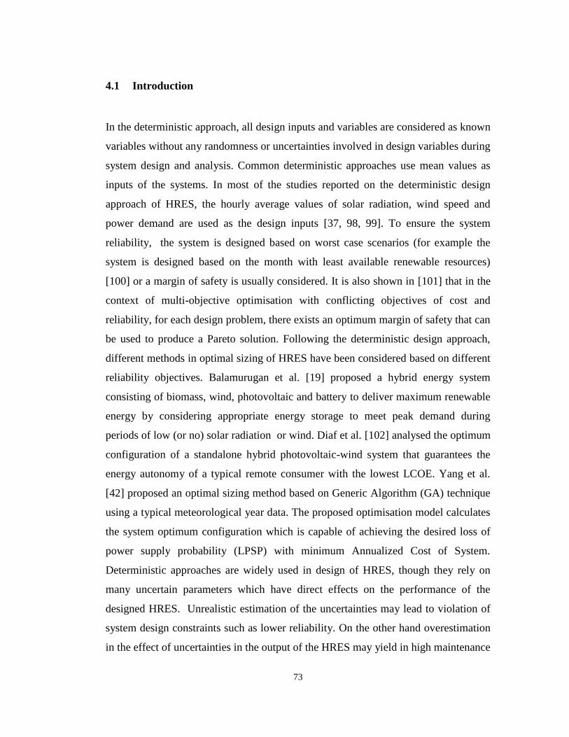
73
4.1 Introduction
In the deterministic approach, all design inputs and variables are considered as known
variables without any randomness or uncertainties involved in design variables during
system design and analysis. Common deterministic approaches use mean values as
inputs of the systems. In most of the studies reported on the deterministic design
approach of HRES, the hourly average values of solar radiation, wind speed and
power demand are used as the design inputs [37, 98, 99]. To ensure the system
reliability, the system is designed based on worst case scenarios (for example the
system is designed based on the month with least available renewable resources)
[100] or a margin of safety is usually considered. It is also shown in [101] that in the
context of multi-objective optimisation with conflicting objectives of cost and
reliability, for each design problem, there exists an optimum margin of safety that can
be used to produce a Pareto solution. Following the deterministic design approach,
different methods in optimal sizing of HRES have been considered based on different
reliability objectives. Balamurugan et al. [19] proposed a hybrid energy system
consisting of biomass, wind, photovoltaic and battery to deliver maximum renewable
energy by considering appropriate energy storage to meet peak demand during
periods of low (or no) solar radiation or wind. Diaf et al. [102] analysed the optimum
configuration of a standalone hybrid photovoltaic-wind system that guarantees the
energy autonomy of a typical remote consumer with the lowest LCOE. Yang et al.
[42] proposed an optimal sizing method based on Generic Algorithm (GA) technique
using a typical meteorological year data. The proposed optimisation model calculates
the system optimum configuration which is capable of achieving the desired loss of
power supply probability (LPSP) with minimum Annualized Cost of System.
Deterministic approaches are widely used in design of HRES, though they rely on
many uncertain parameters which have direct effects on the performance of the
designed HRES. Unrealistic estimation of the uncertainties may lead to violation of
system design constraints such as lower reliability. On the other hand overestimation
in the effect of uncertainties in the output of the HRES may yield in high maintenance

74
costs and [103] shows that calculated costs via a deterministic approach deviate from
the cost obtained by Monte Carlo simulation even without having uncertainty in cost
modelling. Normally obtaining a desired reliability level is considered during design
of a standalone HRES by sizing the battery bank based on worst case scenario which
is non-availability of renewable resources for several days called as days of
autonomy. Conventional reliability measurement methods take into account the
overall performance of the system and do not focus on the time and period of
blackout occurrence.
This chapter focuses on the reliability measures during the design of HRES and
shows the weakness of traditional design method of HRES in maintaining a
satisfactory power generation system even though the overall desired reliability
criteria is been satisfied. The concept block diagram of the designed system in this
study is presented in Figure 1-1. The power supply from wind turbine and PV panels
to the load, the battery bank and dump load follows the priority of first load; second
the battery bank and last the dump load. When the total output of wind turbine and
PV panels is more than load demand and the battery is not fully charged the excess
energy is used to charge the battery and in case that wind turbine and PV panel output
is not enough to cover the load demand the battery will maintain the power shortage.
4.2 Problem formulation and design methodology
The objective is to find the optimum configuration of a standalone HRES with
minimum total cost while satisfying the load demand at the desired reliability level.
The input data would be average hourly or monthly meteorological data of wind
speed and solar irradiance of the desired site along with the average hourly load
demand. Here DPSP , the deficiency of power supply probability is chosen as the
reliability assessment criterion and any configuration of hybrid system which satisfies
above constraint is considered as feasible solution.

75
Here the wind turbine/PV system sizing optimisation is performed following a
deterministic design approach based on exhaustive search. The averages hourly of
weather data and load profile are used as inputs of the design. The power from each
resource is calculated at each time step (every hour) based on the capacity of power
generator.
Conventionally the battery bank is sized prior to wind turbine and PV panels’ sizing.
The size of the battery bank is determined to meet the load demand during autonomy
days, two or three days a year [11]. Following equation estimates the battery bank
size with consideration of maximum depth of discharge, rated battery capacity and
battery life using Equation 3.6.
The performance of whole system is then simulated with :
BatPVWT
PVWTHRESTotal
PPP
PPP
,_
)(
)(
b
a (4.1)
)(a if total power generated by wind turbine and PV is sufficient to cover the load
demand otherwise
)(b where WTP and PVP is not sufficient
and state of charge the battery :
minSOCSOC (4.2)
The reliability of each design candidate can be measured with Equation 4.3 [104]:
8760
1
8760
1
iload
ii
iP
DPS
DPSP (4.3)
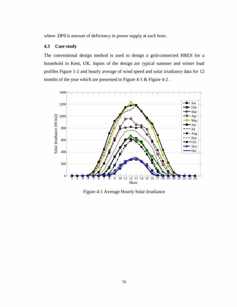
76
where DPS is amount of deficiency in power supply at each hour.
4.3 Case study
The conventional design method is used to design a grid-connected HRES for a
household in Kent, UK. Inputs of the design are typical summer and winter load
profiles Figure 1-2 and hourly average of wind speed and solar irradiance data for 12
months of the year which are presented in Figure 4-1 & Figure 4-2 .
1 2 3 4 5 6 7 8 9 10 11 12 13 14 15 16 17 18 19 20 21 22 23 240
200
400
600
800
1000
1200
1400
Hour
Sola
r Ir
radia
nce
(W
/m2)
Jan
Feb
Mar
Apr
May
Jun
Jul
Aug
Sep
Oct
Nov
Dec
Figure 4-1 Average Hourly Solar Irradiance

77
1 2 3 4 5 6 7 8 9 10 11 12 13 14 15 16 17 18 19 20 21 22 23 240
1
2
3
4
5
6
7
8
9
10
11
12
13
14
15
16
17
18
19
20
Hour
Win
d S
peed (
m/s
)
Jan
Feb
Mar
Apr
May
Jun
Jul
Aug
Sep
Oct
Nov
Dec
Figure 4-2 Average Hourly Wind Speed
Technical and economical characteristics of the system components are given in
Table 1-1.
The battery bank is sized based on three days of autonomy and the overall DPSPof
the system is considered to be less than %1desiredDPSP
Table 4-1 Optimum solution based on common design method
Optimum Solution
WT Rotor Disk
Area (m2)
PV Panel Area
(m2) Number of Batteries DPSP (%) Cost ($)
40.715 0 187 0.4658 124285
78
4.4 Results and Discussion
Through an optimisation method the optimum size of wind turbine and PV panel is
obtained. Table 4-1 presents the optimum sizes of wind turbine rotor disk area, PV
panel area, number of batteries and the overall DPSPof the system. As expected the
optimum size for PV is calculated as zero due to the fact that wind is dominant in the
site under study. Although the optimum solution has DPSPof 0.47% as a system
with high reliability, a more detailed look to the times of power supply deficiency
occurrences and their possible blackout duration shows that this configuration may
not be the most satisfactory solution to the user because majority of power shortages
are most likely to happen very close to each other during the evening in the winter
season.
Figure 4-3 shows a comparison with produced power of HRES and the demand of a
typical day in winter with the possibility of power shortage. The figure shows that the
blackout may actually continue for long hours in this day. From Figure 4-4 it is seen
that in some months when the wind speed is not high enough to produce enough
power to cover the load demand and charge the battery bank long blackouts may
happen even though the battery bank is sized to cover the maximum load level for
three days.
The case study introduced a problem on the common design methods in optimal
sizing of HRES based on a predefined reliability. As a preliminary solution to the
stated problem, adding a constant on the maximum duration of the blackouts is
proposed here. The state of charge (SOC) of the battery can be used as an indicator
for the blackout occurrence. The times when the battery bank is at its maximum depth
of discharge the blackouts are more likely to happen and can be counted as blackout
occurrences. The proposed solution is used to redesign the HRES for desired site in
the case study and new optimum sizes of the HRES components are presented in
Table 4-2.
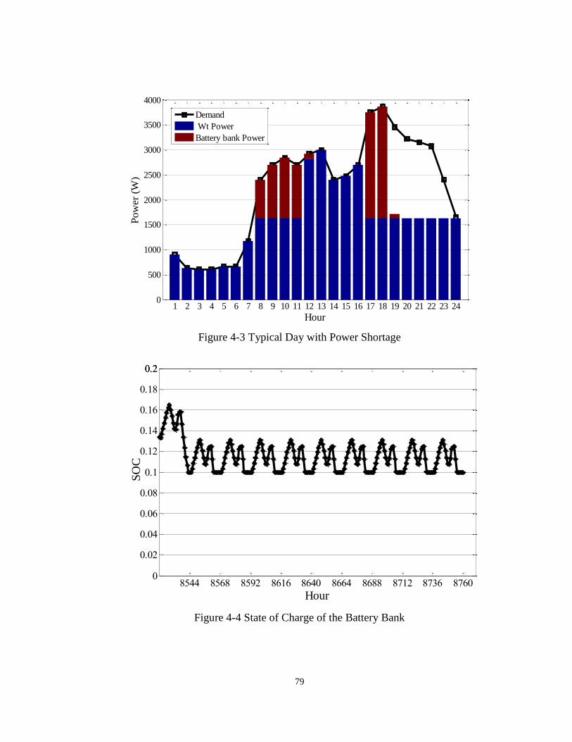
79
Hour
Pow
er
(W)
1 2 3 4 5 6 7 8 9 10 11 12 13 14 15 16 17 18 19 20 21 22 23 240
500
1000
1500
2000
2500
3000
3500
4000
Demand
Wt Power
Battery bank Power
Figure 4-3 Typical Day with Power Shortage
8544 8568 8592 8616 8640 8664 8688 8712 8736 87600
0.02
0.04
0.06
0.08
0.1
0.12
0.14
0.16
0.18
0.20.2
Hour
SO
C
Figure 4-4 State of Charge of the Battery Bank

80
Table 4-2 Optimum solution after adding constraint on maximum blackout hours
Optimum Solution
WT Rotor Disk
Area (m2)
PV Panel Area
(m2) Number of Batteries DPSP (%) Cost ($)
55.418 0 187 0 144045
0 730 1460 2190 2920 3650 4380 5110 5840 6570 7300 8030 87600.9
0.92
0.94
0.96
0.98
1
Hour
Sta
te o
f C
har
ge
of
the
Bat
tery
Ban
k (
SO
C)
8712 8718 8724 8730 8736 8742 8748 8754 8760
0.96
0.965
0.97
0.975
0.98
0.985
0.99
0.995
1
Hour
SO
C
Figure 4-5 State of Charge of the Battery Bank after considering maximum blackout
hours in design
Figure 4-5 shows the state of charge of the battery through the whole year in new
design. Since this value never reaches in the neighbourhood of the maximum depth of
discharge of the battery, the blackouts are very unlikely to happen in the designed
system.

81
4.5 Summary
Traditional reliability measurement criterions in design of HRES only consider the
overall performance of the HRES in design period (for example in a year) and ignore
the time and duration of blackouts occurrences in short times. That is why even
though the designed system has an overall high reliability measure; it may not be
satisfactory as majority of power shortages may happen during a short period.
This study shows that in addition to traditional reliability measurements during the
design a more precise design criterion should be considered in order to prevent design
failures.

82
5 Stochastic design
approach in optimal
sizing of HRES
83
5.1 Introduction
Considering uncertainties when designing the system, could improve the HRES
performance. For that, a realistic method is required to simulate the wind speed and
solar irradiance variations. Different approaches are used to model the renewable
sources behaviour. One of common approaches is fitting the uncertainties to known
distributions such as Weibull or Beta distributions [77]. However researches show
that, for some locations like UK using predefined distributions may not simulate the
weather data properly[105]. Erken [106] used different distributions to find the best
fitted distribution for each hourly meteorological data. Another method in
considering uncertainties is adding a random disturbance to average values of wind
speed and solar irradiance [107]. Lujano-Rojas [76] and Ji [108] used time series
analysis to model wind speed and solar irradiance variations accordingly. Time series
could be a viable solution to model the uncertainties with unknown distributions.
Different methods to integrate the uncertainties in renewable resources in the design
of HRES have been reported. Giannakoudis et al [107] considered adding a known
disturbance to the design inputs to maintain optimum mix of renewable resources.
Nandi and Himri [55, 109] fitted wind speed variation with Weibull distribution.
Lujano-Rojas el al [76] used time series theory to simulate the uncertainties in wind
speed in the design of small wind/battery systems. Usually, the Monte Carlo
simulation approach is used in solving probabilistic problems. Given a significantly
large sample size, this method can provide highly accurate results. However, the main
drawback is the computational burden associated with the large number of repeated
calculations [110]. In addition to the common ‘under uncertainties’ design methods,
the chance constrained programming approach is also a popular method in solving the
problems dealing with random parameters. This method was first introduced by
Charnes and Cooper [78] in 1959. Its main feature is that the resulting decision
ensures the probability of complying with constraints [83]. The chance constrained
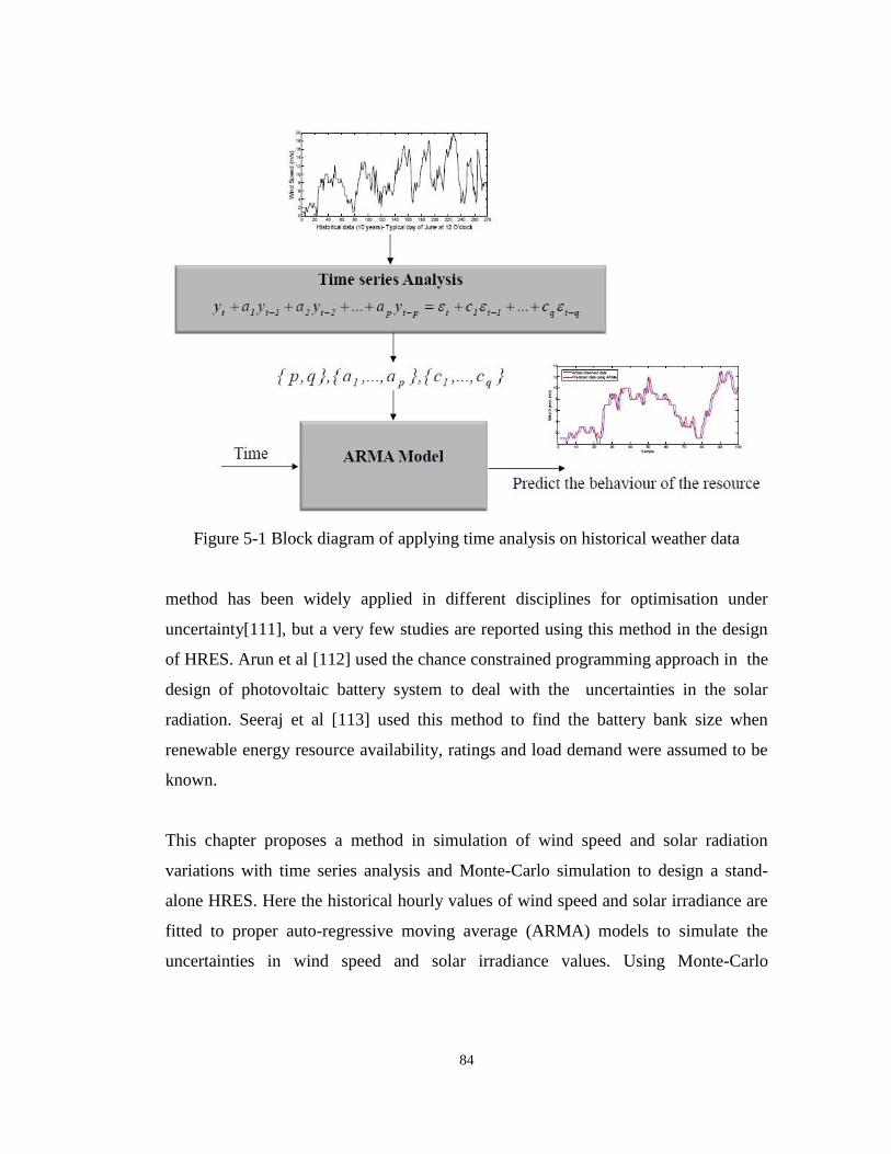
84
Figure 5-1 Block diagram of applying time analysis on historical weather data
method has been widely applied in different disciplines for optimisation under
uncertainty[111], but a very few studies are reported using this method in the design
of HRES. Arun et al [112] used the chance constrained programming approach in the
design of photovoltaic battery system to deal with the uncertainties in the solar
radiation. Seeraj et al [113] used this method to find the battery bank size when
renewable energy resource availability, ratings and load demand were assumed to be
known.
This chapter proposes a method in simulation of wind speed and solar radiation
variations with time series analysis and Monte-Carlo simulation to design a stand-
alone HRES. Here the historical hourly values of wind speed and solar irradiance are
fitted to proper auto-regressive moving average (ARMA) models to simulate the
uncertainties in wind speed and solar irradiance values. Using Monte-Carlo

85
simulation method, design candidates are evaluated based on reliability and the
system total cost. The latter is introduced as the optimum solution.
5.2 The wind speed and solar irradiance simulation model
In this chapter the uncertainties in wind speed and solar irradiance is simulated using
time series method. An ARMA model is fitted to historical meteorological data of
each hour of a typical day of each month of the year. Block diagram of applying time
analysis on historical weather data is presented in Figure 5-1. The output is used to
simulate the variability in wind speed and solar irradiance data of each particular hour
which will be used in Monte-Carlo simulation of design candidates.
5.2.1 Problem formulation and design methodology
The objective is to find the optimum configuration of a standalone HRES with
minimum total cost while satisfying the load demand at the desired reliability level.
The reliability is measures by calculation the deficiency of power supply probability
(DPSP).
The optimisation problem can be formulated as:
MOrepIC CCCTC &min (5.1)
while
desiredDPSPDPSP (5.2)
DPSP is the overall probability of deficiency in annual total power generated by the
hybrid system (Equation 4.3) and any configuration of hybrid system which satisfies
above constraint is considered as feasible solution.
The design variables are the rotor swept area of wind turbine and area of PV panel.
86
The wind turbine rotor area is varied in the range from 0 to 300 m2, PV panels’ area is
from 0 to 175 m2. The battery bank is sized using Equation 3.6.
The performance of whole system is then simulated as:
BatPVWT
PVWTHRESTotal
PPP
PPP
,_
)(
)(
b
a (5.3)
)(a if total power generated by wind turbine and PV is sufficient to cover the load
demand otherwise,
)(b the battery supplies the difference BatP as long as the state of charge the battery
is:
minSOCSOC (5.4)
Considering the uncertainties in renewable resources (modelled using times series
analysis), the reliability of each HRES design candidate is analysed using Monte-
Carlo simulation and the optimum solution with minimum total cost is selected
among design candidates that satisfy the reliability constraint using exhaustive
search.
5.2.2 Case study
The proposed method is used to design a stand-alone HRES for a household in Kent,
UK. The input data for the design are typical summer and winter load profiles which
are presented in Figure 1-2 in addition to historical hourly data of wind speed and
solar irradiance data for 12 months of the year. The ARMA parameters for wind
speed and solar irradiance of each individual hour is estimated based on historical
meteorological data for one typical day of each month. The output of ARMA
simulation is used as hourly wind speed and solar irradiance in Monte-Carlo
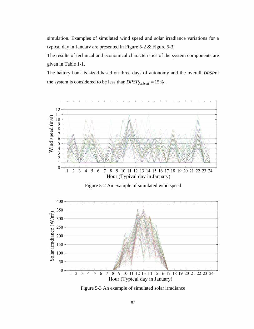
87
simulation. Examples of simulated wind speed and solar irradiance variations for a
typical day in January are presented in Figure 5-2 & Figure 5-3.
The results of technical and economical characteristics of the system components are
given in Table 1-1.
The battery bank is sized based on three days of autonomy and the overall DPSPof
the system is considered to be less than %15desiredDPSP .
1 2 3 4 5 6 7 8 9 10 11 12 13 14 15 16 17 18 19 20 21 22 23 240123456789
10111212
Hour (Typival day in January)
Win
d s
peed
(m
/s)
Figure 5-2 An example of simulated wind speed
1 2 3 4 5 6 7 8 9 10 11 12 13 14 15 16 17 18 19 20 21 22 23 240
50
100
150
200
250
300
350
400
Hour (Typical day in January)
So
lar
irra
dia
nce
(W
/m2)
Figure 5-3 An example of simulated solar irradiance

88
5.2.3 Results and Discussion
In order to investigate the performance of modelling uncertainties with method
explained in Section (5.2.1) in optimal design of HRES, an exhaustive search is
performed to solve the optimisation problem Equation (5.1) the mean value of DPSPs
obtained by performing 10,000 Monte-Carlo simulations on each design candidate is
considered as its overall DPSP and the optimum solution which satisfies the Figure
5-4 compares the upper and lower limits of DPSP values in different configurations
of HRES. The optimum configuration is marked in Figure 5-4 and Table 5-1.
Figure 5-5 & Figure 5-6 show the values and the distribution of DPSP values for the
optimum solution obtained using Monte-Carlo simulation.
The probability of blackout occurrence can be calculated using Monte-Carlo
simulation result. The hours, when the battery bank is at its minimum state of charge
or the overall available power of HRES is less than load demand, are counted as
blackout hours. The probability of blackout occurrence is then calculated with:
sSimulation
BlackoutsHourBlachout
N
nobability ,Pr (5.5)
Figure 5-7 represents the probability of blackout occurrence in each day of the year
for the optimum solution which is calculated with Equation 5.5. The figure clearly
shows that the blackouts have strong probability to happen in the last three months of
the year when renewable resources availability is not high enough to cover the load
demand and charge the battery bank.
Table 5-1 Optimum Configuration
WT Rotor Disk Area (m2) PV Panel Area (m
2) Number of Batteries DPSP (%)
92 150 187 15
Optimum Solution
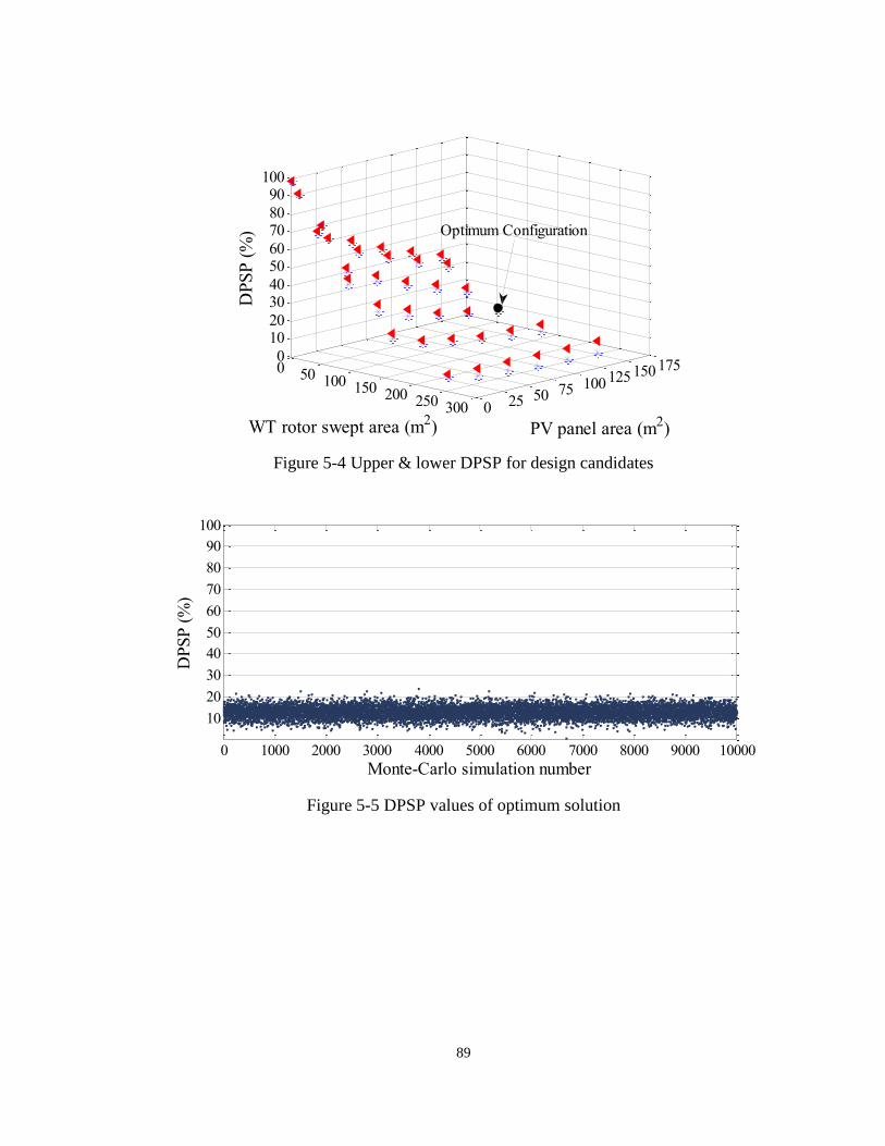
89
0 50 100 150 200 250 300 0 25 50 75 100 125 150 1750
1020
3040
5060
7080
90100
DP
SP
(%
)
PV panel area (m2)WT rotor swept area (m
2)
Optimum Configuration
Figure 5-4 Upper & lower DPSP for design candidates
0 1000 2000 3000 4000 5000 6000 7000 8000 9000 10000
10
20
30
40
50
60
70
80
90
100
Monte-Carlo simulation number
DP
SP
(%
)
Figure 5-5 DPSP values of optimum solution

90
0 5 10 15 20 25 30 35 40 45 50 55 60 65 70 75 80 85 90 95 1000
500
1000
1500
2000
2500
3000
3500
DPDP (%)
Fre
quen
cy
Figure 5-6 Distribution of DPSP values for optimum solution
0 30 60 90 120 150 180 210 240 270 300 330 3600
0.1
0.2
0.3
0.4
0.5
0.6
0.7
0.8
0.9
1
Day number
Bla
cko
ut
pro
bab
ilit
y
Figure 5-7 Probability of blackout occurrence for each day of year
5.2.4 On the Sensitivity Analysis
As the wind turbine and PV panel models presented in Equations 2.1 & 2.11 are
dependent on wind speed and solar irradiance data of desired site and the
unpredictable nature of renewable resources have been considered in stochastic
design approach , performing sensitivity analysis would not result in additional useful
information here.

91
5.2.5 Summary
The Hybrid Renewable Energy System (HRES) can be a reliable solution to bring
electricity to isolated areas where there is no access to the grid by considering
uncertainties in resources at the design stage. Appropriate modelling of wind speed
and solar irradiance variations, at the design stage, would give a more realistic picture
of the designed system performance. This study shows that ARMA models can be
used as a proper method in simulating the wind speed and solar irradiance data in
design of HRES.

92
6 Chance Constrained
Programming Using
Non-Gaussian Joint
Distribution Function in
Design of Standalone
Hybrid Renewable
Energy Systems
93
6.1 Introduction
Performance of a Hybrid Renewable Energy Systems (HRES) is highly affected by
changes in renewable resources and therefore interruptions of electricity supply may
happen in such systems. In this chapter, a method to determine the optimal size of
HRES components is proposed, considering uncertainties in renewable resources.
The method is based on chance-constrained programming (CCP) to handle the
uncertainties in power produced by renewable resources. The design variables are
wind turbine rotor swept area, PV panel area and number of batteries. The common
approach in solving problems with CCP is based on assuming the uncertainties to
follow Gaussian distribution. The analysis presented in this chapter shows that this
assumption may result in a conservative solution rather than an optimum. The
analysis is based on comparing the results of the common approach with those
obtained by using the proposed method. The performance of the proposed method in
design of HRES is validated by using the Monte Carlo simulation approach. To
obtain accurate results in Monte Carlo simulation, the wind speed and solar irradiance
variations are modelled with known distributions as well as using time series
analysis; and the best fit models are selected as the random generators in Monte Carlo
simulation.
Increasing energy demand and depletion of fossil fuel resources have made renewable
energy resources more attractive [114] and advances in technologies had led to
reduced cost, making renewable energy systems competitive with fossil fuels
especially in remote places where grid connection is not available [115].The power
generated from renewable resources is completely dependent on renewable
resources and therefore, largely unpredictable. There are many research works
reported on the assessment of global energy potentials resources [116] and on
investigating the vulnerability of renewable systems and improvement of their
performance. Kalogirou [117] investigated the effect of environmental pollutants and
dust that are transferred with the air on performance of PV panels. Greening [118]
performed an evaluation on the life cycle environmental sustainability of micro-wind
94
turbines in the UK , as compared with grid electricity and solar PV panels. As the
isolated operation (standalone operation) of these power units may not be effective in
terms of cost and reliability [119] unless properly optimised for those qualities. In
recent years there has been an increased interest in the use and optimisation of hybrid
renewable energy systems (HRES) as a viable solution to provide a reliable power
supply, particularly in rural areas with standalone systems [120]. Generally, a HRES
combines two or more energy sources to generate reliable power to satisfy the load
demand at all times and under various weather conditions. Conventionally, the
balance between demand and the system output in standalone systems is obtained by
using an auxiliary power source such as a diesel generator and/or storage such as
battery bank. To ensure an effective use of available renewable energy resources
(wind, sun,...), optimal design and sizing of HRES are essential. The aim is to
optimise the mix of renewable energy systems available to meet the load power
demand, minimise the combined intermittency in power generation, maximize their
contribution to the peak load (thus minimising power generation from the auxiliary
power source)and do this at a minimum cost [121]. That is, using optimal design to
achieve cost effective and reliable HRES. Generally two approaches are followed in
design of HRES; deterministic or stochastic.
In the deterministic approach, all design inputs and variables are considered as known
variables without any randomness involved during system design and analysis.
Common deterministic approaches use mean values as the systems’ inputs and most
of the work reported on the deterministic design approach of HRES implement the
hourly average of solar radiation, wind speed and power demand as the design inputs
[37, 98, 99]. To ensure the system reliability, the system is designed based on worst
case scenarios (for example the system is designed based on the month with least
available renewable resources) [100] or a margin of safety is usually considered.
Stochastic approaches attempt to solve the optimisation problem involving
uncertainties. They deal with uncertainties by using resource functions and chance
95
constraints to transform the stochastic optimisation to an equivalent deterministic
optimisation problem [122]. Chance constrained programming approach is a popular
method in solving the problems dealing with random parameters. The chance
constrained method has been widely applied in different disciplines for optimisation
under uncertainty[111], but a very few studies are reported using this method in the
design of HRES. Arun et al [112] used the chance constrained programming approach
in the design of photovoltaic battery system to deal with the uncertainties in the
solar radiation. Seeraj et al [113] used this method to find the battery bank size when
renewable energy resource availability, ratings and load demand were assumed to be
known. For simplicity the power produced by photovoltaic array and wind turbines
are assumed to follow a bivariate normal distribution with known mean and standard
deviation.
In this chapter, the chance constrained programming approach is used to design a
standalone hybrid wind turbine/PV and battery bank system. The design variables are
the rotor swept area of wind turbine, area of photovoltaic panel and the size of battery
bank. However, assuming normal distribution as the joint distribution of produced
power by wind turbine and PV panel may not result in a realistic output of the
system. Therefore, in this study the joint distribution of the wind turbine and PV
panel output power is considered to follow an unknown distribution and individual
cumulative distribution function (CDF) of the produced power by wind turbine and
PV panel. The CDF, corresponding to each hour of typical days of 12 months of the
year, is calculated based on the hourly historical data of wind speed and solar
irradiance. The design candidates are constrained in satisfying the load demand,
which is achieved when the overall probability of the load demand to be satisfied is
more than a certain value. The design candidates satisfying the reliability constraints
are evaluated by their total cost. The design candidate with minimum total cost is
defined as the optimum configuration. The reliability of the design output is validated
through Monte Carlo simulation. As the performance of Monte Carlo simulation is
directly dependent on the accuracy of its random data generator, two common

96
methods in modelling wind speed and solar irradiance variations are used to deal with
this. These methods are the time series analysis and fitting historical data to the
known distributions. They are performed on historical meteorological data of the
desired site and the statistical characteristic of their output is compared to the
observed data in order to ensure accurate modelling of wind speed and solar
irradiance variation in the Monte Carlo simulation. The performance of the proposed
design method is demonstrated in the design of an HRES for a household in Kent,
UK, as explained in section 6.3.
The concept block diagram of the designed system used in this study is shown in
Figure 1-1. The power generated from the wind turbine and PV panels follows the
supply priority of first load; second the battery bank and last the dump load. When
the total output of wind turbine and PV panels is more than load demand and the
battery is not fully charged the excess energy is used to charge the battery. When the
wind turbine and PV panel output is not enough to cover the load demand, the battery
will supply the difference.
The development of this chapter is presented as follows:
The components modelling and cost modelling are presented in chapter 2.
Problem formulation and design methodology are presented in section 6.2 and a case
study is described in section 6.3.
Validation with Monte Carlo simulation is described in section 6.4 and finally
conclusions are presented in section 6.5.
6.2 Problem formulation and design methodology
The methodology of finding the optimum size of a standalone wind
turbine/PV/Battery bank following a stochastic approach is discussed in this section.
The objective is to find the optimum configuration of a standalone HRES with

97
minimum total cost while satisfying the load demand at the desired reliability level.
The objective function can be formulated as:
treplacemenMOICNAA
CCCTCBatPVWT
&,,
min (6.1)
The energy balance of the system can be simulated with:
BatPVWT
PVWTHRES
PPP
PPP
,
)(
)(
b
a (6.2)
)(a if total power generated by wind turbine and PV is sufficient to cover the load
demand, otherwise
)(b when WTP + PVP is not sufficient to meet the demand and the battery supplied
the difference.
As mentioned before, ignoring the uncertainties in wind speed and solar irradiance
leads to unreliable supply system. The design of HRES under uncertainties can be
generally described as a nonlinear stochastic optimisation problem. Using the chance
constrained programming the optimisation problem of optimal sizing of HRES can be
defined as:
treplacemenMOICNAA CCCBatPVWT
&,,min (6.3)
s.t.
8760,...,2,1,)Pr( iDemandP ii (6.4)
minSOCSOC (6.5)
where
8760,...,2,1, iPPPPii BatiPVWTi (6.6)

98
Here the values of power generated by the wind turbine and PV system are dependent
random variables following known distributions and the power of battery bank is
dependent random variable. The historical hourly data of wind speed and solar
irradiance are used to estimate the joint cumulative distribution function (CDF) of the
power produced by the wind turbine and PV system at each time step (each hour) of
calculation. The load demand is assumed to be deterministic and known at each time
step and is the reliability of compliance of the constraint or confidence level given
as:
1001 DPSP (6.7)
where DPSP of each design candidate which is calculated as Equation 4.3.
The probabilistic constraint in Equation 6.4 can to be changed to a deterministic
constraint as follows:
))(Pr( 1t
CVSOCSOCDemandPP BatBat
tttPVWT tt (6.8)
1))(Pr( 1t
CVSOCSOCDemandPP BatBat
tttPVWT tt (6.9)
The number of batteries for a given wind turbine rotor area and PV panel area can be
obtained by solving Equation 6.9 which requires the calculation of joint CDF of WT
and PV panel output powers at each hour.
To solve Equarion 6.9, two approaches are followed: the common method used in
previous studies and a new method proposed in this chapter.
6.2.1 Common method used in previous studies-Using normal distribution
To solve Equation 6.9, tWTP and tPVP at each hour are assumed to follow normal
Gaussian distribution with mean values of tWTP ,
tPVP and standard deviations
tWTP , tPVP [113].
99
The sum of tWTP and
tPVP is assumed to have a new random variable tP with mean
value of tP and the variance
2
tP such that:
tWTtPVt PPP (6.10)
tWTtPVtWTtPVtWTtPVt PPPPPPP ,222 2 (6.11)
where tWTtPV PP , is coefficient of correlation between
tWTP and tPVP at each hour.
The deterministic equivalent of Equation 6.9 is expressed as:
Zt
cVSOCSOCDemand
tt PPBatBat
ttt
)( 1 (6.12)
where Z is the inverse of the cumulative normal probability distribution
corresponding to the required reliability of compliance of the constraint or confidence
level , .Equation 6.12 is used to obtain the minimum battery size for each
configuration of WT and PV panel and the configuration with minimum cost is
selected as the best design.
6.2.2 The proposed method
In the proposed method, it is assumed that WTP and PVP are independent random
variables following known distributions (Weibull and Beta distributions, accordingly)
and the joint cumulative distribution function of these is calculated as:
PVWTPVWT PPPP FFF ., (6.13)
Equation 6.9 can be re-written as:

100
)1()( 1,1
PVWT PPBatBat
ttt Ft
cVSOCSOCDemand (6.14)
Equation 6.14 is a deterministic constraint which can be satisfied by calculating the
inverse of the joint cumulative distribution function of wind turbine and PV panel
power, corresponding to the required reliability of compliance of the constraint .
The values of WT and PV panel output powers are used to obtain the minimum
battery size for each configuration of WT and PV panel and the configuration with
minimum cost is selected as the best design. The performance of the proposed
method is validated using Monte Carlo simulation.
The flowchart of the design and validation process is presented in Figure 6-1.
6.3 Case study
The chance constrained programming is used to design a standalone HRES for a
household in Kent, UK. The input data for the design are historical hourly data (2000-
2008) of wind speed and solar irradiance for 12 months of the year together with
typical summer and winter load profiles shown in Figure 1-2. The two methods
explained in section 6.2 are used to find the optimum solution for the desired location
and the results obtained with two methods are compared for five different confidence
levels from 0.1 to 0.5.
Details of technical and economical characteristics of the system components are
given in Table 1-1.
The system under study consists of a wind turbine, a PV panel and a battery bank.
The wind turbine rotor area is varied in the range from 0 to 154 m2, PV panels’ area is
from 0 to 260 m2 and minimum number of batteries required to meet the probabilistic
constraint is determined for each case. Upper limits of each renewable power
generation unit is calculated assuming that it is the only source of power. The number

101
of batteries is assumed to vary from 0 to 478. The maximum permitted number of
batteries in the study is calculated, using Equation 3.6, considering required storage
for one day of autonomy for a day with highest daily load demand; here typical
winter load demand is used.
Figure 6-2 shows a sample contour plot for different values obtained by calculating
the joint CDF of WTP and PVP for a typical day in August at 12.00 noon using the
method proposed in this chapter.
The optimum configurations and their total costs, obtained with the two methods
explained in section 6.2 for five different confidence levels from 0.1 to 0.5 are
presented in Table 6-1. As shown in this table, the results of the two methods are
close in lower reliability; lower ; but as the reliability increases the difference
between total costs of optimum solutions of the two methods becomes more
significant. Figure 6-3 compares the total cost of the optimum solutions of the two
methods for five values of .Figure 6-4 shows a three dimensional space formed by
the wind turbine rotor swept area, PV panel area and minimum battery capacity
required to meet the load, using the two design methods for value of 0.8. As can be
seen from the figure, using the method proposed in this chapter results in a bigger
design space as compared with using the normal Gaussian distribution, which leads to
a larger number of feasible optimum solutions. Figure 6-5 and Figure 6-6 show a 3D
view of feasible design options based on different number of batteries for each of the
two design methods explained in sections 4.1 and 4.2, for value of 0.8. As the
objective function in the defined optimisation problem of Equation 6.3 is the present
value of total cost, the optimum solution of each method is selected based on having
minimum total cost and is marked in Figure 6-5 and Figure 6-6.

102
Table 6-1 The comparison between results obtained using two design methods
WT Rotor Area (m2) PV Panel Area (m
2) Number of Batteries Total Cost ($) WT Rotor Area (m
2) PV Panel Area (m
2) Number of Batteries Total Cost ($)
0.5 50 113 0 61 174,413 116 0 61 178,091
0.6 40 128 0 61 195,103 134 0 61 202,919
0.7 30 149 0 61 222,688 154 17 61 245,237
0.8 20 154 69 61 292,193 154 139 61 354,801
0.9 10 154 234 61 440,887 154 260 421 598,285
Optimum Solutions Obtained Using Proposed MethodDPSP (%)α
Optimum Solutions Obtained Using Normal Distrobution
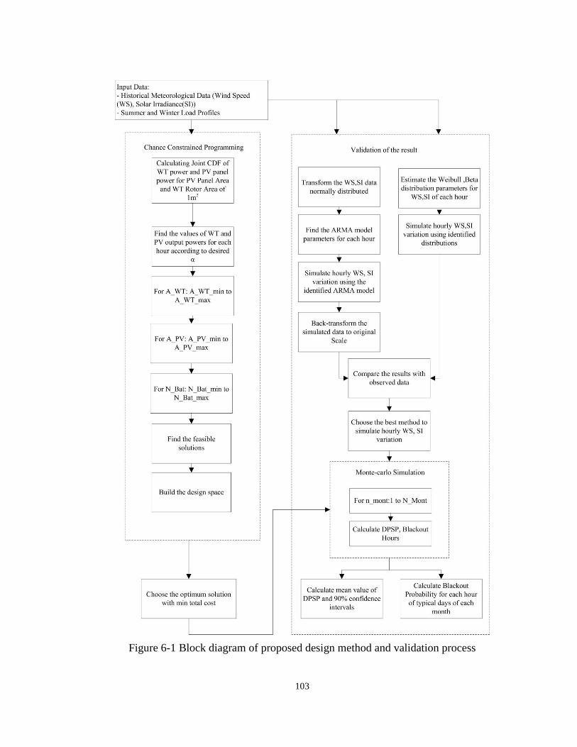
103
Figure 6-1 Block diagram of proposed design method and validation process
104
6.4 Validation with Monte Carlo simulation
Monte Carlo simulation is used to validate the reliability of the optimum solution
obtained with the proposed method as well as comparing the performance of the
optimum solutions marked in Figure 6-5 and Figure 6-6 as the optimum solution of
two discussed methods. The performance of the Monte Carlo simulation is dependent
on the accurate modelling of the uncertainties in the wind speed and solar irradiance.
Different approaches are used to model the renewable sources behaviour. One of the
common approaches is by fitting the uncertainties to known distributions such as
Weibull or Beta distributions [77]. However, research show that for some locations
(e.g. in the UK), using predefined distributions may not simulate the weather data
properly[105]. Erken [106] used different distributions to find the best fitted
distribution for each hourly meteorological data. Another method in considering
uncertainties is adding a random disturbance to average values of wind speed and
solar irradiance [107]. Lujano-Rojas [76] and Ji [108] used time series analysis to
model wind speed and solar irradiance variations, accordingly. To obtain the most
accurate model in wind speed and solar irradiance variations of the desired location,
two different methods are used for fitting the historical data to known distributions
and time series analysis using autoregressive moving average models (ARMA)
explained in chapter5. The results obtained by using ARMA simulation are compared
with the results obtained from fitting the historical data of wind speed to Weibull
distribution and solar irradiance to Beta distribution and then calculating the mean
squared error (MSE) of each method as:
h
iii YY
hMSE
1
2)ˆ(1
(6.15)
where iY is the mean value of vector of simulated values and iY is the mean value of
vector of observed values for hour no i . Calculated values of MSE for desired site
show that wind speed variation is best fitted to Weibull distribution than ARMA
105
model. The MSE of the simulation with Weibull distribution is 0.0007 which is
significantly lower than that for ARMA simulation which is 0.27. However for solar
radiation simulation, the ARMA model performs better than Beta distribution with
MSE of 6.94 as compared to 36.24. It can be seen that the values of MSE are
considerably bigger for solar radiation than for wind speed. It should be noted that the
values of solar radiation calculated are mostly in the range of 100 to 600 and wind
speed changes in the range between 2 to 5.5. Figure 6-7 & Figure 6-10 present the
result of comparison between the mean values of simulated data and observed values.
The Monte Carlo simulation is repeated as long as the statistical characteristics of the
modelled variation in wind speed and solar radiation are close enough to the actual
observed data. The reliability of optimum solution obtained using the proposed
method; marked in Figure 6-5 is then estimated as the mean of the results obtained
over the number of the simulation; 5000 times. Figure 6-11 compares the DPSP
values obtained at each run of simulation, its mean value and 90% confidence
intervals of the results. The overall DPSP of the optimum configuration which is
calculated as the mean value of DPSP values obtained from Monte Carlo simulation.
If we consider as 1001 DPSP and calculate based on the results from Monte
Carlo simulation; the results show that the optimum solution obtained by using the
method proposed in this chapter complies with the design constraint which requires
an overall load satisfaction with a probability of ; here = 0.8.
Monte-Carlo simulation is also used to compare the performance of optimum
solutions obtained using each of explained methods in terms of blackout occurrence
probability as well as the average excess power that is produced by the wind turbine
and PV panel in case of choosing either of these optimum solutions and the results
are presented in Figure 6-12 and Figure 6-13. The probability of blackout occurrence
for each hour for a typical day of each month is shown in Figure 6-12. This figure
shows that the probability of blackout occurrence in each hour of the optimum
solution obtained by proposed method is less that 18%. The Figure 6-12 also shows
that the probability of blackout for both optimum solutions is higher in the last three

106
months of the year. Also the value of this probability does not differ significantly
between two optimum solutions for each particular month. However the amount of
average daily excess power shown in Figure 6-13 proves that the proposed method
results in less conservative design option as compared to the output of common
method as there is less excess power produced by wind turbine and PV panel in the
output design of this method.
6.5 Summary
This chapter suggests the use of the chance constrained programming in the design of
HRES. To solve the chance constrained problem two methods are compared:
The common approach which solves the problem based on the assumption of
the uncertain variables following the normal Gaussian distribution
A new method is proposed in this chapter to solve the chance constrained
problem without initial assumption on the type of joint distribution of two
uncertain variables; wind speed and solar irradiance.
Analysis of comparing the results obtained in this study shows that by using the first
method some feasible configurations are ignored and the output configuration of the
design may not be the best configuration.
A case study, design of a standalone hybrid wind /PV /battery bank system is
presented for a farm in Kent, UK. The outcome of the design is validated based on
deficiency of power supply probability through performing Monte Carlo simulation.
Historical meteorological data of the desired location is used to find the best method
in modelling wind speed and solar irradiance variations. This is done by comparing
the statistical characteristics of fitting the variations to known distributions as well as
using time series analysis; ARMA models. It is shown that, for the desired location,
the Weibull distribution is the best fitted model for wind speed variation and that
ARMA model performs better in modelling solar radiation variations. However it
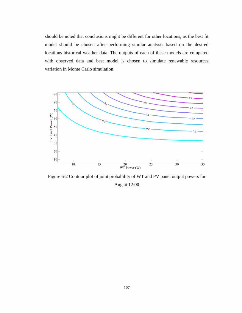
107
should be noted that conclusions might be different for other locations, as the best fit
model should be chosen after performing similar analysis based on the desired
locations historical weather data. The outputs of each of these models are compared
with observed data and best model is chosen to simulate renewable resources
variation in Monte Carlo simulation.
0.2
0.2
0.20.2
0.4
0.4
0.4
0.6
0.6
0.8
WT Power (W)
PV
Pan
el P
ow
er (
W)
10 15 20 25 30 35
10
20
30
40
50
60
70
80
90
Figure 6-2 Contour plot of joint probability of WT and PV panel output powers for
Aug at 12:00
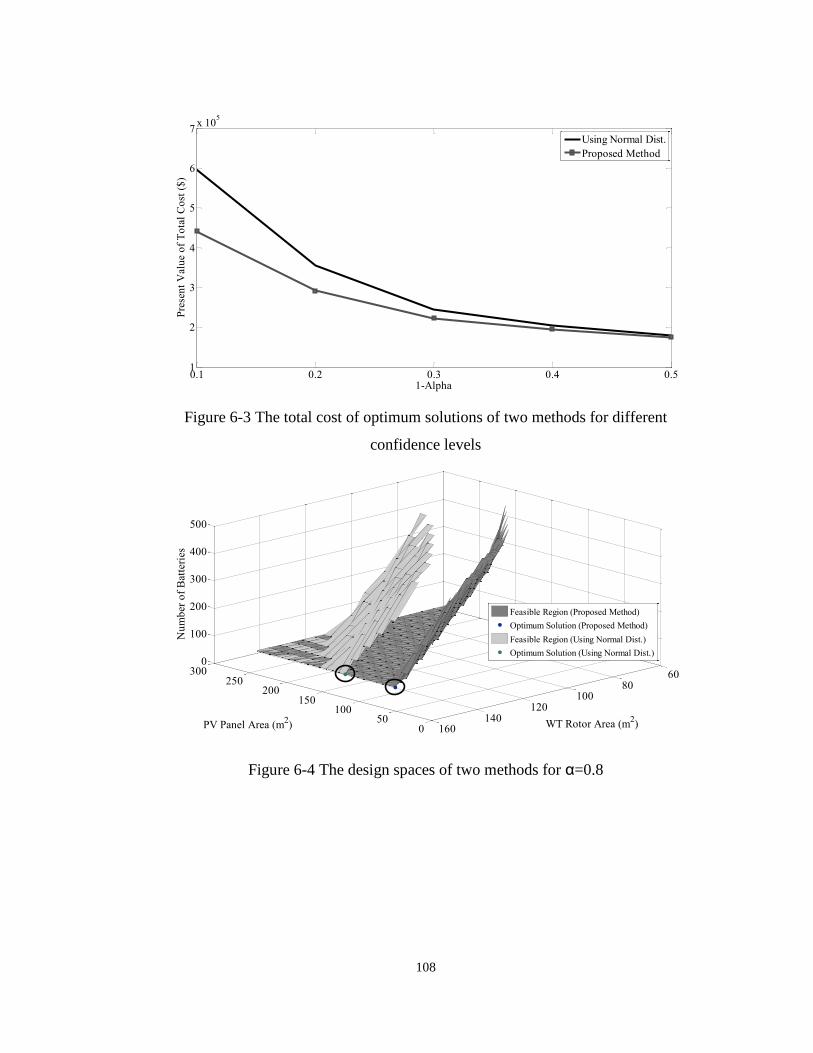
108
0.1 0.2 0.3 0.4 0.51
2
3
4
5
6
7x 10
5
1-Alpha
Pre
sen
t V
alu
e o
f T
ota
l C
ost
($
)
Using Normal Dist.
Proposed Method
Figure 6-3 The total cost of optimum solutions of two methods for different
confidence levels
050
100150
200250
300 6080
100120
140160
0
100
200
300
400
500
WT Rotor Area (m2)PV Panel Area (m
2)
Nu
mb
er o
f B
atte
ries
Feasible Region (Proposed Method)
Optimum Solution (Proposed Method)
Feasible Region (Using Normal Dist.)
Optimum Solution (Using Normal Dist.)
Figure 6-4 The design spaces of two methods for α=0.8
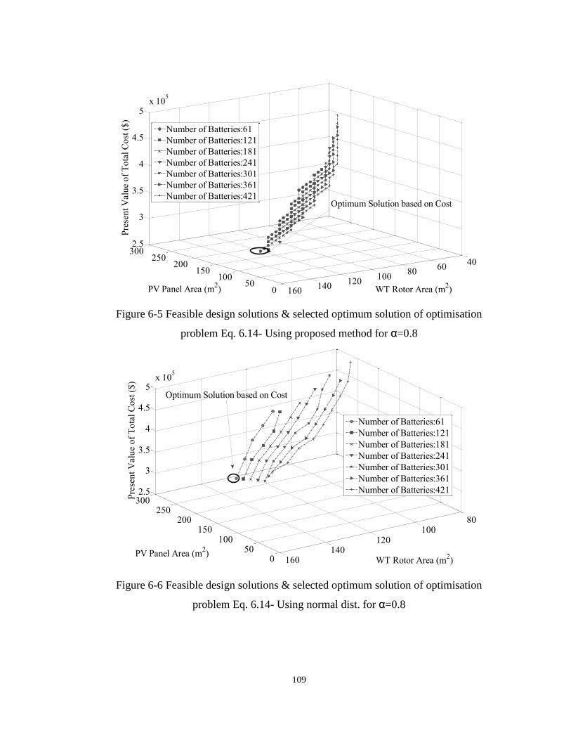
109
050
100150
200250
300
4060
80100
120140
160
2.5
3
3.5
4
4.5
5x 10
5
PV Panel Area (m2)
Pre
sen
t V
alu
e o
f T
ota
l C
ost
($
)Number of Batteries:61
Number of Batteries:121
Number of Batteries:181
Number of Batteries:241
Number of Batteries:301
Number of Batteries:361
Number of Batteries:421
WT Rotor Area (m2)PV Panel Area (m
2)
Optimum Solution based on Cost
Figure 6-5 Feasible design solutions & selected optimum solution of optimisation
problem Eq. 6.14- Using proposed method for α=0.8
050
100150
200250
300
80100
120140
160
2.5
3
3.5
4
4.5
5x 10
5
Pre
sen
t V
alu
e o
f T
ota
l C
ost
($
)
Number of Batteries:61
Number of Batteries:121
Number of Batteries:181
Number of Batteries:241
Number of Batteries:301
Number of Batteries:361
Number of Batteries:421
WT Rotor Area (m2)
PV Panel Area (m2)
Optimum Solution based on Cost
Figure 6-6 Feasible design solutions & selected optimum solution of optimisation
problem Eq. 6.14- Using normal dist. for α=0.8
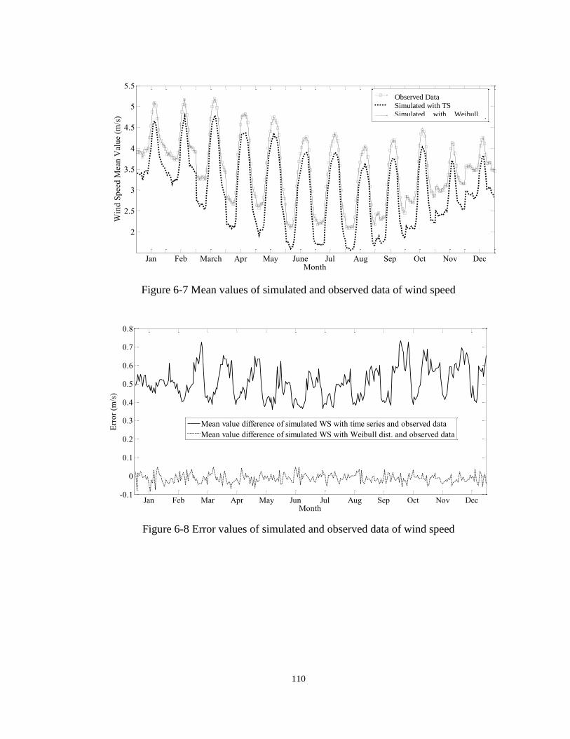
110
Jan Feb March Apr May June Jul Aug Sep Oct Nov Dec
2
2.5
3
3.5
4
4.5
5
5.5
Month
Win
d S
pee
d M
ean
Val
ue
(m/s
)
Onserved Data
Simulated with TS
Simulated with Weibull Dist.
Figure 6-7 Mean values of simulated and observed data of wind speed
Jan Feb Mar Apr May Jun Jul Aug Sep Oct Nov Dec-0.1
0
0.1
0.2
0.3
0.4
0.5
0.6
0.7
0.8
Month
Err
or
(m/s
)
Mean value difference of simulated WS with time series and observed data
Mean value difference of simulated WS with Weibull dist. and observed data
Figure 6-8 Error values of simulated and observed data of wind speed
Observed Data
Simulated with TS Simulated with Weibull
Dist
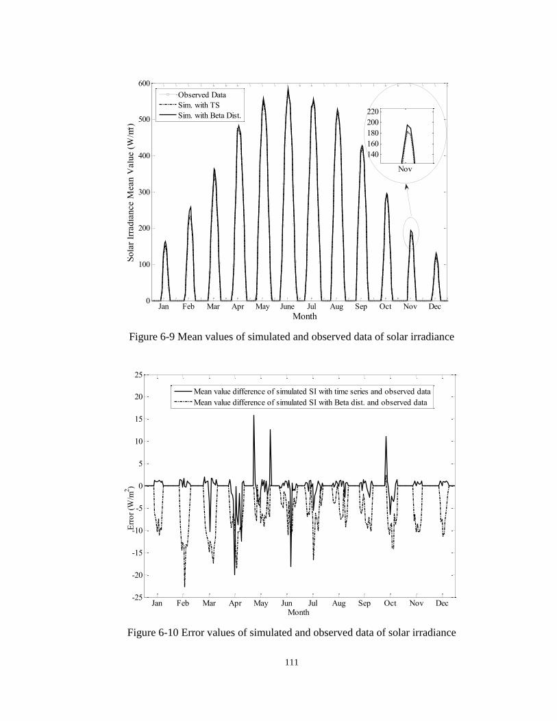
111
Jan Feb Mar Apr May June Jul Aug Sep Oct Nov Dec0
100
200
300
400
500
600
Month
Sola
r Ir
radia
nce M
ean V
alu
e (
W/m
2)
Observed Data
Sim. with TS
Sim. with Beta Dist.
Nov
140
160
180
200
220
Figure 6-9 Mean values of simulated and observed data of solar irradiance
Jan Feb Mar Apr May Jun Jul Aug Sep Oct Nov Dec-25
-20
-15
-10
-5
0
5
10
15
20
25
Month
Err
or
(W/m
2)
Mean value difference of simulated SI with time series and observed data
Mean value difference of simulated SI with Beta dist. and observed data
Figure 6-10 Error values of simulated and observed data of solar irradiance

112
0 500 1000 1500 2000 2500 3000 3500 4000 4500 5000
2
4
6
8
10
12
14
16
18
20
Simulation
DP
SP
(%
)
DPSP
90% Confidence Intervals
Mean Value of DPSP
Figure 6-11 Deficiency of power supply probability of optimum solution obtained
with Monte Carlo simulation
Jan Feb Mar Apr May Jun Jul Aug Sep Oct Nov Dec0
2
4
6
8
10
12
14
16
18
Month
Pro
bab
ilit
y o
f B
lack
ou
t (%
)
Probability of Blackout at each Hour of Typical Days-
Optimum solution (Using Normal Dist.)
Probability of Blackout at each Hour of Typical Days-
Optimum solution (Proposed Method)
Figure 6-12 Comparison between probability of blackout occurrences of two
optimum solutions for α=0.8
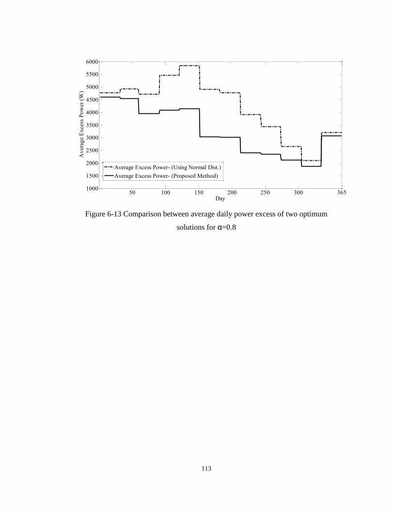
113
50 100 150 200 250 300 3651000
1500
2000
2500
3000
3500
4000
4500
5000
5500
6000
Day
Av
erag
e E
xce
ss P
ow
er (
W)
Average Excess Power- (Using Normal Dist.)
Average Excess Power- (Proposed Method)
Figure 6-13 Comparison between average daily power excess of two optimum
solutions for α=0.8

114
7 Multi-Objective Design
under Uncertainties of
Hybrid Renewable
Energy System Using
NSGA-II and Chance
Constrained
Programming

115
7.1 Introduction
The optimum design of Hybrid Renewable Energy Systems (HRES) depends on
different economic, environmental and performance related criteria which are often
conflicting objectives. The Non-dominated Sorting Genetic Algorithm (NSGA-II)
provides a decision support mechanism in solving multi-objective problems and
providing a set of non-dominated solutions where finding an absolute optimum
solution is not possible. The present study uses NSGA-II algorithm in the design of a
standalone HRES comprising wind turbine, PV panel and battery bank with the
(economic) objective of minimum system total cost and (performance) objective of
maximum reliability. To address the uncertainties in renewable resources (wind speed
and solar irradiance), an innovative method is proposed which is based on Chance
Constrained Programming (CCP). A case study is used to validate the proposed
method, where the results obtained are compared with the conventional method of
incorporating uncertainties using Monte Carlo simulation.
Decision making problems can be categorized in two classes based on the number of
objective functions that are involved in the problem; single objective and multi-
objective. In a single objective problem, the aim is to identify the best solution
corresponding to minimising or maximising a single objective function. However, in
real life, the decision making process usually involves more than one objective
function. Multi-objective problems do not have a single optimal solution but they
have a set of compromised solutions between different objective functions known as
Pareto set.
In optimal sizing of HRESs, there is normally more than one objective function to be
considered. Two important objective functions in the design of a HRES are cost and
reliability. Since these objectives are contradicting, a single optimal solution cannot
be found (with minimum cost and maximum reliability) and a multi-objective
optimisation is needed to find a trade-off; Pareto set solutions. Several studies have
116
been reported in multi-objective optimisation of HRES considering different
objection functions and using various optimisation techniques.
Genetic Algorithms (GA) proved to be popular in solving optimisation problems.
Ould [41] proposed a Pareto-based multi-objective GA for sizing a hybrid solar–
wind-battery system with the aim of minimising the annualized cost and minimising
the probability of loss of power supply. Montoya et al. [53] presented a hybrid
Pareto- based multi-objective meta-heuristic approach to minimise voltage deviations
and power losses in power networks, which can be extended to hybrid systems. Yang
et al. [42] proposed a GA based optimal sizing technique using typical meteorological
yearly data. The proposed optimisation model determines the system optimum
configuration which is able to provide the desired Loss of Power Supply Probability
(LPSP) with minimum Annualized Cost.
The Non-dominated Sorting Genetic Algorithm (NSGA-II) was proposed [46] to
perform multi-objective evolutionary algorithms (MOEA) in which an elite-
preserving operator gives the best individuals the opportunity to be directly
transferred to the next generation. By doing so, a ‘good’ solution which is found in
early generations is never removed from the population unless a better solution is
discovered. Katsigiannis [20] used the NSGA-II to design a small autonomous hybrid
power system that contained both renewable and conventional power sources with the
objectives of minimising the energy cost of the system and total greenhouse gas
emission during the system life time. However, the effects of uncertainties in
renewable energy generation were not considered in this study.
Different methods to include the uncertainties in renewable resources in the design of
HRES have been reported. Giannakoudis et al [107] considered adding a known
disturbance to the design inputs to maintain optimum mix of renewable resources.
Nandi et al.[55] assumed that wind speed variation follows the Weibull distribution.
Lujano-Rojas el al [76] used time series theory to simulate the uncertainties in wind
117
speed in the design of small wind/battery systems. Usually, the Monte Carlo
simulation approach is used in solving probabilistic problems. Given a significantly
large sample size, this method can provide highly accurate results. However, the main
drawback is the computational burden associated with the large number of repeated
calculations [110]. The Chance Constrained Programming (CCP) approach, first
introduced by Charnes and Cooper [78] in 1959, is now popular method in solving
problems that include random parameters. Its main feature is that it ensures the
probability of the resulting decision to comply with the specified constraints [83].
The CCP method has been widely applied in different disciplines for optimisation
under uncertainty[111], but very few studies are reported on using this method for the
design of HRES. Arun et al. [112] used the CCP approach in the design of a PV-
battery system to deal with the uncertainties in the solar radiation. Seeraj et al. [113]
used this method to find the battery bank size when renewable energy resource
availability, ratings and load demand were assumed to be known.
This chapter presents the results of a multi-optimisation NSGA-II based approach for
the design of a standalone HRES, shown in Figure 1-1, considering uncertainties in
the resources available. The approach employs the chance constrained programming
to deal with the effects of uncertainties in renewable resources instead of common
approach of using Monte Carlo simulation. It is shown in Chapter 6 that chance
constrained programming can result in optimum solution for a predefined reliability
in a single-objective optimisation problem in design of HRES, however in a multi-
objective optimisation problem where there is no predefined reliability,
conventionally Monte Carlo simulation is employed. This study proposes a novel
method in employing chance constrained programming in multi-objective problems
as a substitute of Monte Carlo simulation. The study proposes a method in which
chance constrained programing is used as a tool in estimating the expected value of
the objective function which is affected by the uncertainties, in other words instead of
finding the optimum solution for a predefined value of reliability, chance constrained
programing is used to estimate the expected value of the reliability of the design

118
candidates in a multi-objective optimisation problem. To evaluate the performance of
the proposed method, the results obtained are compared with those obtained by
employing the Monte Carlo simulation.
The outline of this chapter is as follows:
The components modelling and cost modelling are presented in chapter 2.
Problem formulation and design methodology are presented in section 7.2.
A case study is described in section 7.5. Results and discussion are described in
section 7.6 and finally conclusions are presented in section 7.7.
7.2 Problem formulation and design methodology
The proposed technique adopts the non-dominated sorting genetic algorithm (NSGA-
II) [46] in combination with the chance constrained programming (CCP) [78] to
effectively solve the multi-objective optimisation problem of design of a HRES under
uncertainties. The aim is to find the Pareto set solutions based on the desired
objective functions using NSGA-II. The NSGA-II provides a very efficient procedure
in keeping the elitism optimisation process as well as preserving the diversity which
assures a good convergence towards the Pareto-optimal front without losing the
solution diversity [47].
The following steps are implemented in the NSGA-II algorithm.
1: Initial population is generated based on defined decision variables and number of
populations.
2: Evaluation of each chromosome in terms of defined objective functions. The
adopted methods in evaluation the objective functions affected by uncertainties are
explained in sub-section (7.3) and (7.4).
3: Set the generation count
4: Prepare the mating pool
5: Perform crossover and mutation operators
6: Perform non-dominated sorting
119
7: Calculate the crowding distance
8: Perform the selection based on rank. If individuals with the same rank are
encountered, crowding distance is compared. A lower rank and higher crowding
distance is the selection criteria.
9: Increment the generation count and repeat steps 4 to 8 until the counter reaches the
maximum number of generation
The decision variables are the wind turbine rotor swept area ( WTA ), the PV panel area
( PVA ) and the number of batteries ( BatN ).
The optimisation problem can be defined as:
DPSPTCBatPVWT NAA ,min ,, (7.1)
s.t.
minSOCSOC (7.2)
where
treplacemenMOIC CCCTC & (7.3)
As Equation 7.1 shows, two objective functions have been considered associated with
both minimisation of the system total cost (TC ) and the deficiency of power supply
probability ( DPSP ); where DPS is the amount of power shortage at each hour and h
is the total hours under study.
The energy balance of the system can be modelled as:
BatPVWT
PVWTHRES
PPP
PPP
,
)(
)(
b
a (7.4)
)(a if total power generated by the wind turbine and PV is sufficient to cover the load
demand, otherwise
)(b WTP + PVP is not sufficient to meet the demand and the battery has to supply the
difference.
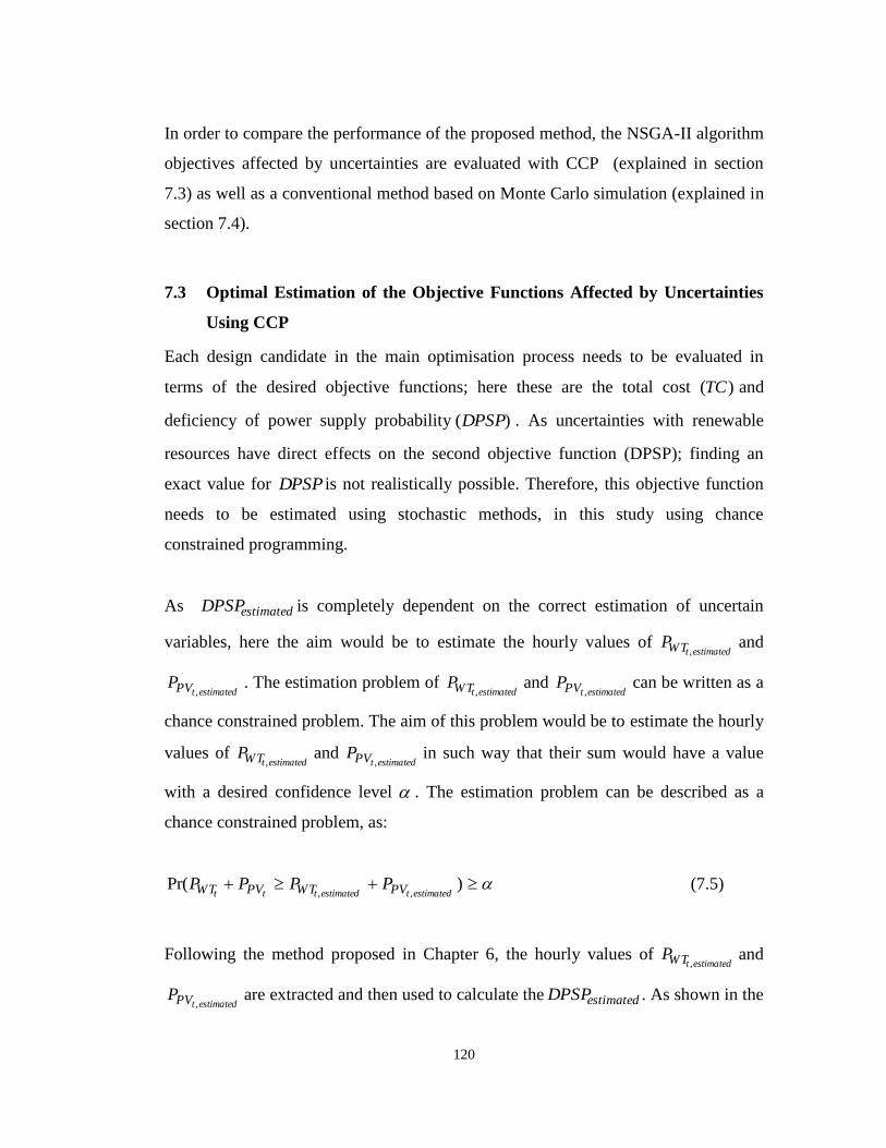
120
In order to compare the performance of the proposed method, the NSGA-II algorithm
objectives affected by uncertainties are evaluated with CCP (explained in section
7.3) as well as a conventional method based on Monte Carlo simulation (explained in
section 7.4).
7.3 Optimal Estimation of the Objective Functions Affected by Uncertainties
Using CCP
Each design candidate in the main optimisation process needs to be evaluated in
terms of the desired objective functions; here these are the total cost )(TC and
deficiency of power supply probability )(DPSP . As uncertainties with renewable
resources have direct effects on the second objective function (DPSP); finding an
exact value for DPSP is not realistically possible. Therefore, this objective function
needs to be estimated using stochastic methods, in this study using chance
constrained programming.
As estimatedDPSP is completely dependent on the correct estimation of uncertain
variables, here the aim would be to estimate the hourly values of estimatedtWTP
,and
estimatedtPVP,
. The estimation problem of estimatedtWTP
,and
estimatedtPVP,
can be written as a
chance constrained problem. The aim of this problem would be to estimate the hourly
values of estimatedtWTP
,and
estimatedtPVP,
in such way that their sum would have a value
with a desired confidence level . The estimation problem can be described as a
chance constrained problem, as:
)Pr(,, estimatedtestimatedttt PVWTPVWT PPPP (7.5)
Following the method proposed in Chapter 6, the hourly values of estimatedtWTP
,and
estimatedtPVP,
are extracted and then used to calculate the estimatedDPSP . As shown in the

121
case study , this method requires considerably shorter process time as compared with
the conventional Monte Carlo simulation.
7.4 Monte Carlo Simulation
Monte Carlo simulation is conventionally used to estimate the expected value of the
parameters with uncertainties. The performance of the Monte Carlo simulation is
dependent on the accurate modelling of uncertainties in the wind speed and solar
irradiance. Different approaches are used to model the renewable sources. One of the
common approaches is by fitting the uncertainties to known distributions such as
Weibull or Beta distributions [77]. However, research show that for some locations
(e.g. in the UK), using predefined distributions may not simulate the weather data
properly[105]. Erken [106] used different distributions to find the best fitted
distribution for each hourly meteorological data. Another method in considering
uncertainties is adding a random disturbance to the average values of wind speed and
solar irradiance [107]. Lujano-Rojas [76] and Ji [108] used a time series analysis to
model wind speed and solar irradiance variations. To obtain accurate modelling of
wind speed and solar irradiance variations, two methods are used to correlate
historical data to known distributions and time series analysis using autoregressive
moving average models (ARMA). Based on the location of the desired site, the
performance of different modelling methods should be investigated and the most
suitable model selected as the random data generator to model the uncertainties in
Monte Carlo simulation. Using these random data generators, the Monte Carlo
simulation is repeated enough for each configuration until the expected values of the
objective function; here DPSPE , is calculated with the confidence level of %90 and
variation value of less than %3. The confidence level in Monte Carlo simulation is
estimated using

122
Table 7-1 Monte Carlo simulation parameters
Confidence
Level (%)99.75 99 98 96 95.5 95 90 80 68
Confidence
Coefficient
(Zc)
3 2.58 2.33 2.05 2 1.96 1.645 1.28 1
NZUL c
),( (7.6)
Where the L and U are the lower and upper values of the estimation, and are the
mean value and standard deviation of the simulation results, cZ is the confidence
coefficient and N the number of the repeatation of the Monte Carlo simulation. The
relevant values of cZ to different confidence levels are presented in Table 7-1.
7.5 Case study
The proposed method is used to design a standalone HRES for a household in Kent,
UK. The input data for the design are historical hourly data (2000-2008) of wind
speed and solar irradiance for 12 months of the year together with typical summer
and winter load profiles shown in Figure 1-2. The load profile is a typical load profile
in the UK which is adopted from [84].
Details of technical and economical characteristics of the system components are
given in Table 1-1.
The system under study consists of a wind turbine, a PV panel and a battery bank.
The wind turbine rotor area is varied in the range from 0 to 154 m2 (in 10 steps), PV
panels area is from 0 to 260 m2 and minimum number of batteries required to meet
the probabilistic constraint is determined for each case. The number of batteries is
assumed to vary from 0 to 478. The maximum permitted number of batteries in this
study is calculated, using Equation 3.6, considering required storage for one day of
autonomy with highest daily load demand; here typical winter load demand is used.

123
The NSGA-II algorithm is performed for 250 iterations with a population number of
100, the mating pool size is considered as 0.5 of the population, crossover probability
pc = 0.9 and mutation probability of n1 ; where n is the number of variables; here 3.
To select the best model for wind speed and solar irradiance in Monte Carlo
simulation, the results of ARMA simulation are compared with those obtained from
fitting the historical data of wind speed to Weibull distribution and solar irradiance to
Beta distribution. Based on the results presented in Chapter 6 Weibull distribution
showed better performance in modelling wind speed variation and ARMA simulation
is used to model solar irradiance in the desired site.
7.6 Results and discussion
The system under study was designed based on the methodologies explained in
section 7.2 and results are presented in this section.
Figure 7-1-a and Figure 7-2-a present a comparison between the initial populations
and the final Pareto sets of performing NSGA-II in combination with CCP and
Monte Carlo simulation. It can be observed that the NSGA-II with CCP produces
more conservative results as compared to the other method, as it results in solutions
with higher total cost. However, it obtains better results in high reliabilities close to
100%; with lower total cost of the system.Figure 7-1-b and Figure 7-2-b show how
the output of each technique converges to its final Pareto set. As can be seen, in both
cases (using the CCP and Monte Carlo simulation), the outputs of the NSGA-II
converges to the final Pareto set at generation 150.
The final Pareto sets of performing optimisation process using proposed NSGA-II
algorithm on the site under study; in combination with CCP as well as Monte Carlo
simulation are compared in Figure 7-3. The Pareto sets obtained in both cases of
employing NSGA-II are well defined and solutions are spread over the reliability
axis. It should be noted that a solution with zero total cost is not feasible. Although
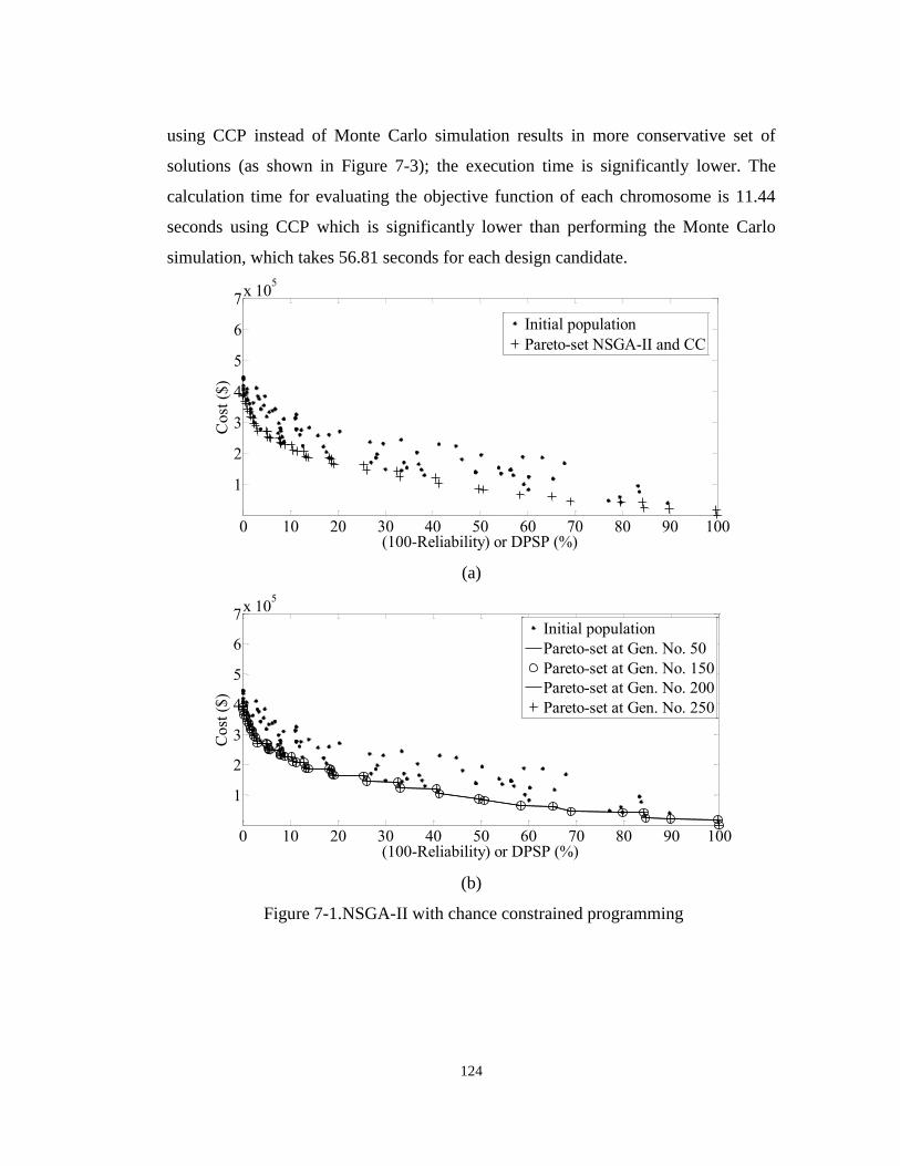
124
using CCP instead of Monte Carlo simulation results in more conservative set of
solutions (as shown in Figure 7-3); the execution time is significantly lower. The
calculation time for evaluating the objective function of each chromosome is 11.44
seconds using CCP which is significantly lower than performing the Monte Carlo
simulation, which takes 56.81 seconds for each design candidate.
0 10 20 30 40 50 60 70 80 90 100
1
2
3
4
5
6
7x 10
5
(100-Reliability) or DPSP (%)
Co
st (
$)
Initial population
Pareto-set NSGA-II and CC
(a)
0 10 20 30 40 50 60 70 80 90 100
1
2
3
4
5
6
7x 10
5
(100-Reliability) or DPSP (%)
Co
st (
$)
Initial population
Pareto-set at Gen. No. 50
Pareto-set at Gen. No. 150
Pareto-set at Gen. No. 200
Pareto-set at Gen. No. 250
(b)
Figure 7-1.NSGA-II with chance constrained programming

125
0 10 20 30 40 50 60 70 80 90 100
1
2
3
4
5
6
7x 10
5
(100-Reliability) or DPSP (%)
Cost
($)
Initial population
Pareto-set NSGA-II and Monte Carlo Sim.
(a)
0 10 20 30 40 50 60 70 80 90 100
1
2
3
4
5
6
7x 10
5
(100-Reliability) or DPSP (%)
Co
st (
$)
Initial population
Pareto-set at Gen. No. 50
Pareto-set at Gen. No. 150
Pareto-set at Gen. No. 200
Pareto-set at Gen. No. 250
(b)
Figure 7-2 NSGA-II with Monte Carlo simulation
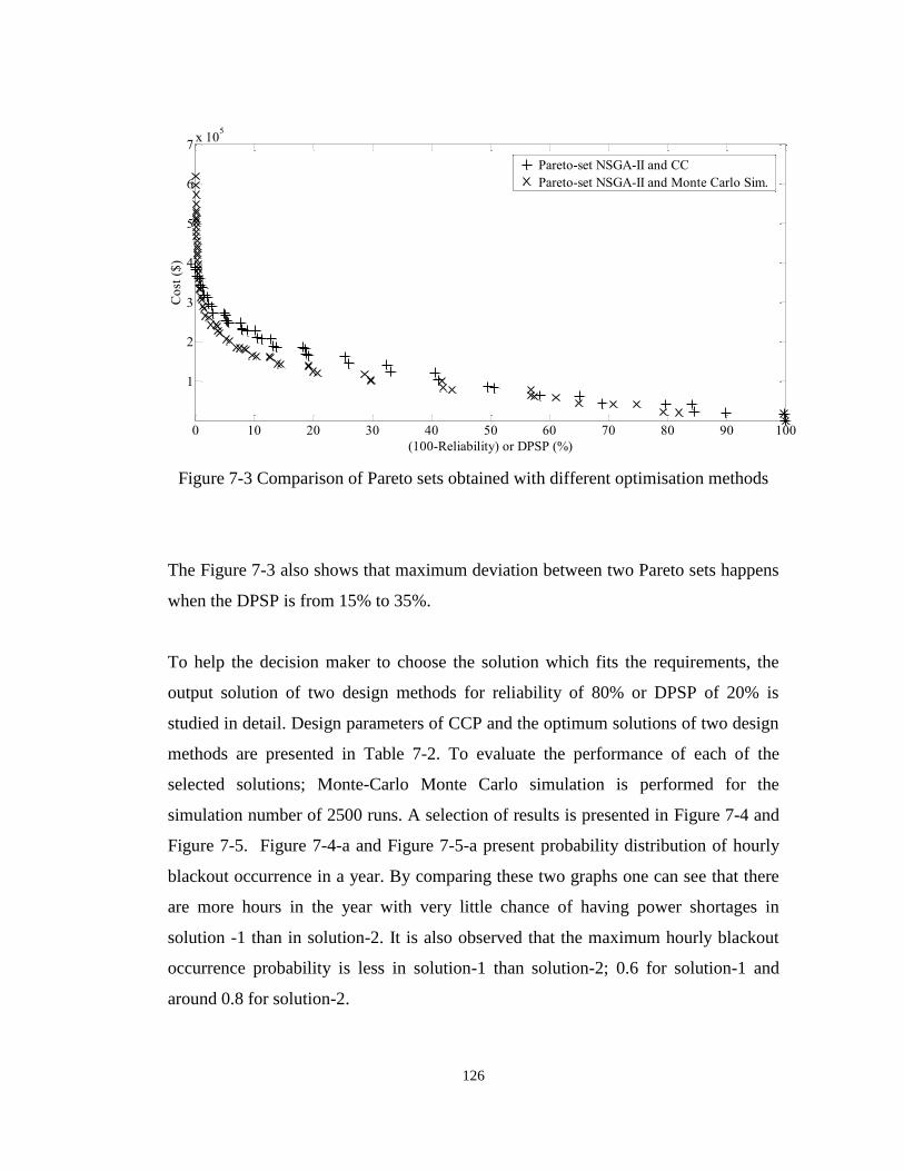
126
0 10 20 30 40 50 60 70 80 90 100
1
2
3
4
5
6
7x 10
5
(100-Reliability) or DPSP (%)
Co
st (
$)
Pareto-set NSGA-II and CC
Pareto-set NSGA-II and Monte Carlo Sim.
Figure 7-3 Comparison of Pareto sets obtained with different optimisation methods
The Figure 7-3 also shows that maximum deviation between two Pareto sets happens
when the DPSP is from 15% to 35%.
To help the decision maker to choose the solution which fits the requirements, the
output solution of two design methods for reliability of 80% or DPSP of 20% is
studied in detail. Design parameters of CCP and the optimum solutions of two design
methods are presented in Table 7-2. To evaluate the performance of each of the
selected solutions; Monte-Carlo Monte Carlo simulation is performed for the
simulation number of 2500 runs. A selection of results is presented in Figure 7-4 and
Figure 7-5. Figure 7-4-a and Figure 7-5-a present probability distribution of hourly
blackout occurrence in a year. By comparing these two graphs one can see that there
are more hours in the year with very little chance of having power shortages in
solution -1 than in solution-2. It is also observed that the maximum hourly blackout
occurrence probability is less in solution-1 than solution-2; 0.6 for solution-1 and
around 0.8 for solution-2.

127
Table 7-2 Optimum solutions of two design methods for reliability=0.8
WT Rotor Area (m2) PV Panel Area (m2) Number of Batteries WT Rotor Area (m2) PV Panel Area (m2) Number of Batteries
0.9 92 26 49 77 0 96
NSGA-II and MonteCarlo simulation (Solution-2)NSGA-II and chance constrained programming (Solution-1)
α
Figure 7-4-b and Figure 7-5-b present the average daily probability of blackout
occurrence throughout the year. Comparing these to figures shows that in solution-1
the last three months of the year have the highest probability of blackout occurrence
which is due higher load demand in winter (see Figure 1-2) as well as less renewable
resources available in these months. However, in solution-2 the second half of the
year has higher probability of power loss.
The day that has the largest probability of blackout occurrence in Figure 7-4-b and
Figure 7-5-b is selected and details of having blackout at each hour of that day is
presented in Figure 7-4-c and Figure 7-5-c.
Figure 7-4-d and Figure 7-5-d show the results of performing Monte Carlo simulation
for 2500 times on the hour with most probability of blackout and presents the
frequency and load satisfaction percentage for that hour.
128
0 0.1 0.2 0.3 0.4 0.5 0.6 0.7 0.8 0.9 11
1000
2000
3000
4000
5000
6000
7000
8000
Probability of blackout occurrence
Nu
mb
er o
f h
ou
rs
(a)
0 50 100 150 200 250 300 365
0.1
0.2
0.3
0.4
0.5
0.6
0.7
0.8
0.9
1
Day No.
Pro
bab
ilit
y o
f bla
ckout
occ
urr
ence
(b)
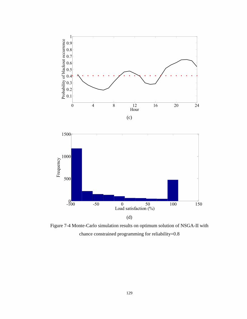
129
0 4 8 12 16 20 24
0.1
0.2
0.3
0.4
0.5
0.6
0.7
0.8
0.9
1
Hour
Pro
bab
ilit
y o
f b
lack
ou
t o
ccu
rren
ce
(c)
-100 -50 0 50 100 1500
500
1000
1500
Load satisfaction (%)
Fre
quen
cy
(d)
Figure 7-4 Monte-Carlo simulation results on optimum solution of NSGA-II with
chance constrained programming for reliability=0.8
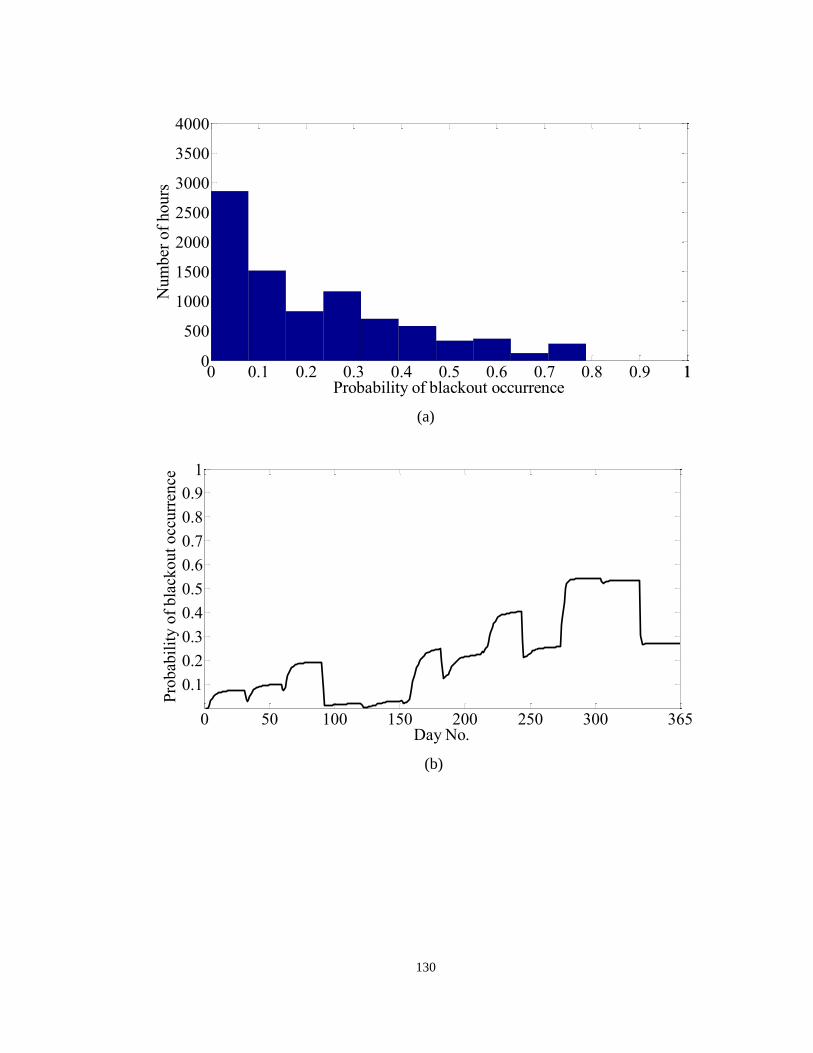
130
0 0.1 0.2 0.3 0.4 0.5 0.6 0.7 0.8 0.9 110
500
1000
1500
2000
2500
3000
3500
4000
Probability of blackout occurrence
Num
ber
of
hours
(a)
0 50 100 150 200 250 300 365
0.1
0.2
0.3
0.4
0.5
0.6
0.7
0.8
0.9
1
Day No.
Pro
bab
ilit
y o
f bla
ckout
occ
urr
ence
(b)

131
0 4 8 12 16 20 24
0.1
0.2
0.3
0.4
0.5
0.6
0.7
0.8
0.9
1
Hour
Pro
bab
ilit
y o
f b
lack
ou
t o
ccu
rren
ce
(c)
-100 -50 0 50 100 1500
500
1000
1500
Load satisfaction (%)
Fre
qu
ency
(d)
Figure 7-5 Monte-Carlo simulation results on optimum solution of NSGA-II with
Monte Carlo simulation for reliability=0.8
7.7 Summary
This chapter proposes a multi-objective optimisation algorithm for optimum
economic and reliability oriented design of hybrid renewable energy system. The
algorithm takes into account the uncertainties in renewable resources. The decision

132
variables are the wind turbine rotor swept area, the PV panel area and the number of
batteries. Two conflicting objectives which are total cost and system reliability are
considered. A novel method in using chance constrained programming is proposed in
this study to estimate the expected value of the objective function; the reliability of
design candidate; affected by uncertain values of wind speed and solar irradiance at
each jour under study. This reduces the evaluation time of the design candidate and
consequently the run time of the NSGA-II program.
The results obtained by using the proposed methods are compared with those
obtained using a conventional Monte Carlo simulation. The comparison shows that
the proposed method yields conservative results in lower reliability values and better
results in high reliability values.

133
8 Summary and
Conclusion
134
This dissertation work comprised a study on optimum design of hybrid renewable
energy systems including wind turbine, PV panels and battery bank. This dissertation
work involved investigating different design methods; deterministic and stochastic
optimization techniques; components modeling and formulating the uncertainties.
This chapter summarizes main contributions of the work as well as point directions
for further research in this area.
8.1 Original contribution
The thesis contributes to the following domains:
Design of grid-connected HRES considering a back-up storage
Investigation on the reliability of deterministic design approach
Modelling the variation of power coefficient of the wind turbine.
Modelling the uncertainties of renewable resources
Optimal design of HRES under uncertainties.
Multi objective optimal design of HRES under uncertainties
The obtained results are discussed in more detail throughout the following
subsections.
8.1.1 Design of grid-connected HRES considering a back-up storage
Conventional grid-connected HRES rely on grid to obtain the required amount of
electricity they require to satisfy the load demand in case of deficit in produced
power. However new concepts in buying electricity from grid at different prices at
different hours requires development of new design methods in grid-connected HRES
This study proposed an investigation on the possibility of adding a small storage
system to cover the electricity shortage during peak hours. Through a sample case
study it is shown that depending on the grid electricity price it might be economically

135
more profitable to consider adding a small storage to HRES to maintain the shortage
at the peak hours.
8.1.2 Investigation on the reliability of deterministic design approach
It is shown that by considering the overall values of traditional reliability criterions
during the design some valuable and essential reliability information might be
ignored and the outcome of the design may not be able to perform satisfactory. It is
shown that in order to prevent the design failures, additional detail performance
evaluations are required to be considered on top of the usual reliability measurements
during the design of the system.
8.1.3 Modelling the variation of power coefficient of the wind turbine
Since in this work the focus is on optimal sizing of HRES based on the penetration of
the renewable resources and specific type of components are not necessarily chosen,
to obtain a mathematical model independent of the type of the wind turbine the power
curve of the different wind turbines are used to calculate the corresponding Cp value
to different wind speeds and through an least square optimisation a best fitted
mathematical model is found to model the wind turbine power coefficient variations
at different wind speed values. This model is particularly created for use in case
studies reported in this thesis and the input data for the modelling is extracted from
wind turbines in response to the demand of the load used in the case study.
8.1.4 Modelling the uncertainties of renewable resources
The Hybrid Renewable Energy System (HRES) can be a reliable solution to bring
electricity to isolated areas where there is no access to the grid by considering
uncertainties in resources at the design stage. Appropriate modelling of wind speed
and solar irradiance variations, at the design stage, would give a more realistic picture
of the designed system performance and would result in more reliable HRES. The
precision in modelling uncertainties would reduce the economic effect of over design
of the system which might have been caused because of over estimation of the

136
uncertainties. Monte Carlo simulation is proven to perform well in design under
uncertainties however its performance is completely dependent n its random data
generator. To obtain the most accurate model in wind speed and solar irradiance
variations of the desired location, two different methods are used for fitting the
historical data to known distributions and time series analysis using autoregressive
moving average models (ARMA) The results obtained by using ARMA simulation
are compared with the results obtained from fitting the historical data of wind speed
to Weibull distribution and solar irradiance to Beta distribution. Comparing the
statistical characteristics of the generated data by mentioned methods it is shown that
the random data generator to model the uncertainties in Monte Carlo simulation
should be selected based on the location of the desired site.
8.1.5 Optimal design of HRES under uncertainties using CCP
Chance-constrained problems are performing well in solving optimisation problems
involving uncertainties. However they are conventionally solved based on an initial
assumption that is the uncertainties to follow Gaussian distribution. Though the
performed analysis in this work it is shown that this assumption may result in a
conservative solution rather than an optimum. This thesis proposes a analytical
method in solving chance constrained programming with unknown joint distribution
of the random variables. It also shows that by using the common approach the design
space would be smaller than the design space obtained by the proposed method and
therefore the outcome of the common method is more conservative. Though by using
proposed method can obtain a less conservative yet equally reliable HRES.
8.1.6 Multi objective optimal design of HRES under uncertainties
Many of the reported researched on optimal design of HRES in the literature are
either single objective or they are ignoring the resource uncertainties. In this work
two contradicting objectives; cost and reliability are selected and NSGA-II is used as
the base for performing the multi objective optimisation. The work also proposes a
novel method in employing chance constrained programming in multi-objective

137
problems as a substitute of Monte Carlo simulation in estimating the expected value
of the objective function which is affected by the uncertainties, in other words instead
of finding the optimum solution for a predefined value of reliability, chance
constrained programing is used to estimate the expected value of the reliability of the
design candidates in a multi-objective optimisation problem.
8.2 Critical appraisal and future works
The techniques and results, presented throughout this thesis, can be possibly
improved as the objectives of the following future research directions.
The economic and demand parameters are considered as deterministic values.
Considering the uncertainties in the economic aspect such as inflation and interest
rates can be done in future works. The unpredictable nature of the demand especially
for small sites can also be taken into account in future improvements.
Adding other renewable sources such as ground source can be considered in further
researches.
138
List of Publications
A. Kamjoo, A. Maheri, G. A. Putrus, and A. M. Dizqah, ”Optimal Sizing of
Grid-Connected Hybrid Wind-PV Systems with Battery Bank Storage,” in
World Renewable Energy Forum (WREF), 2012
Kamjoo, A., A. Maheri, and G. Putrus, ” Reliability Criteria in Optimal Sizing
of Stand-alone Hybrid Wind-PV-Battery bank System,” Environment
Friendly Energies and Applications (EFEA) Symposium, 2012
Kamjoo, A., A. Maheri, and G. Putrus, ”Wind Speed and Solar Irradiance
Variation Simulation Using ARMA Models in Design of Hybrid Wind-PV
Battery System,” Journal of Clean Energy Technologies, 2013.1: p. 14-17
Kamjoo, A., A. Maheri, and G.A. Putrus, ”Chance constrained programming
using non-Gaussian joint distribution function in design of standalone hybrid
renewable energy systems,” Energy, 2014. 66(0): p. 677-688
Kamjoo, A. Maheri, A. M. Dizqah, and G. A. Putrus, ”Multi-Objective
Design Under Uncertainties of Standalone Hybrid Renewable Energy System
Using NSGAII and Chance Constrained Programming,” Electrical Power and
Energy Systems,01/ 2016; 74; 187-194
A.M. Dizqah, A. Maheri, K. Busawon, and A. Kamjoo, ”Modeling and
Simulation of Standalone Solar Power Systems,” International Journal of
Computational Methods and Experimental Measurements 01/2014; 2(1):107-
125 / WIT Press Journals
A.M. Dizqah, A. Maheri, K. Busawon, A. Kamjoo, ”A Multivariable Optimal
Energy Management Strategy for the Standalone DC Microgrids,” IEEE
Transactions on Power Systems, ,PP(99):1-10,
DOI:10.1109/TPWRS.2014.2360434 (Open-Access)
139
References
[1] Santoyo-Castelazo E, Azapagic A. Sustainability assessment of energy systems: integrating
environmental, economic and social aspects. Journal of Cleaner Production. 2014;80:119-38.
[2] Koroneos C, Fokaidis P, Moussiopoulos N. Cyprus energy system and the use of renewable energy
sources. Energy. 2005;30(10):1889-901.
[3] Weisser D. Power sector reform in small island developing states: what role for renewable energy
technologies? Renewable and Sustainable Energy Reviews. 2004;8(2):101-27.
[4] Bahaj AS, Myers L. Analytical estimates of the energy yield potential from the Alderney Race
(Channel Islands) using marine current energy converters. Renewable Energy. 2004;29(12):1931-45.
[5] Chen F, Duic N, Manuel Alves L, Carvalho M. Renewislands-Renewable energy solutions for
islands. Renewable and Sustainable Energy Reviews. 2007;11(8):1888-902.
[6] Ahmad S, Kadir MZAA, Shafie S. Current perspective of the renewable energy development in
Malaysia. Renewable and Sustainable Energy Reviews. 2011;15(2):897-904.
[7] Dursun E, Kilic O. Comparative evaluation of different power management strategies of a stand-
alone PV/Wind/PEMFC hybrid power system. International Journal of Electrical Power & Energy
Systems. 2012;34(1):81-9.
[8] Fadaee M, Radzi MAM. Multi-objective optimization of a stand-alone hybrid renewable energy
system by using evolutionary algorithms: A review. Renewable and Sustainable Energy Reviews.
2012;16(5):3364-9.
[9] Shaahid SM, Elhadidy MA. Technical and economic assessment of grid-independent hybrid
photovoltaic-diesel-battery power systems for commercial loads in desert environments. Renewable
and Sustainable Energy Reviews. 2007;11(8):1794-810.
[10] Yang H, Wei Z, Chengzhi L. Optimal design and techno-economic analysis of a hybrid solar-
wind power generation system. Applied Energy. 2009;86(2):163-9.
[11] Deshmukh MK, Deshmukh SS. Modeling of hybrid renewable energy systems. Renewable and
Sustainable Energy Reviews. 2008;12(1):235-49.
[12] Mellit A, Benghanem M, Kalogirou SA. Modeling and simulation of a stand-alone photovoltaic
system using an adaptive artificial neural network: Proposition for a new sizing procedure. Renewable
Energy. 2007;32(2):285-313.
[13] Straatman PJT, van Sark WGJHM. A new hybrid ocean thermal energy conversion Offshore solar
pond (OTEC-OSP) design: A cost optimization approach. Solar Energy. 2008;82(6):520-7.
[14] Løken E. Use of multicriteria decision analysis methods for energy planning problems.
Renewable and Sustainable Energy Reviews. 2007;11(7):1584-95.
[15] Pohekar SD, Ramachandran M. Application of multi-criteria decision making to sustainable
energy planning—A review. Renewable and Sustainable Energy Reviews. 2004;8(4):365-81.
[16] Wang J-J, Jing Y-Y, Zhang C-F, Zhao J-H. Review on multi-criteria decision analysis aid in
sustainable energy decision-making. Renewable and Sustainable Energy Reviews. 2009;13(9):2263-
78.
[17] J.L. C. Multiobjective programming and planning. Academic Press, New York. 1978.
[18] Garcia RS, Weisser D. A wind-diesel system with hydrogen storage: Joint optimisation of design
and dispatch. Renewable Energy. 2006;31(14):2296-320.
[19] Balamurugana P AS, Jose TL. Optimal operation of biomass/wind/PV hybrid energy system for
rural areas. International Journal of Green Energy. 2009;6(1):104–16.
[20] Katsigiannis YA, Georgilakis PS, Karapidakis ES. Multiobjective genetic algorithm solution to
the optimum economic and environmental performance problem of small autonomous hybrid power
systems with renewables. Renewable Power Generation, IET. 2010;4(5):404-19.
[21] Kaabeche A, Belhamel M, Ibtiouen R. Sizing optimization of grid-independent hybrid
photovoltaic/wind power generation system. Energy. 2011;36(2):1214-22.
[22] Mahor A, Prasad V, Rangnekar S. Economic dispatch using particle swarm optimization: A
review. Renewable and Sustainable Energy Reviews. 2009;13(8):2134-41.
140
[23] Kashefi Kaviani A, Riahy GH, Kouhsari SM. Optimal design of a reliable hydrogen-based stand-
alone wind/PV generating system, considering component outages. Renewable Energy.
2009;34(11):2380-90.
[24] Avril S, Arnaud G, Florentin A, Vinard M. Multi-objective optimization of batteries and hydrogen
storage technologies for remote photovoltaic systems. Energy. 2010;35(12):5300-8.
[25] Hakimi SM, Tafreshi SMM, Kashefi A. Unit Sizing of a Stand-alone Hybrid Power System Using
Particle Swarm Optimization (PSO). Conference Unit Sizing of a Stand-alone Hybrid Power System
Using Particle Swarm Optimization (PSO). p. 3107-12.
[26] Lee TY. Wind-photovoltaic capacity coordination for a time-of-use rate industrial user. IET
Renewable Power Generation. 2009;3(2):152.
[27] Kirkpatrick S, Gelatt C, Vecchi M. Optimization by simulated annealing. Science. 1983;220:671-
80.
[28] Giannakoudis G, Papadopoulos AI, Seferlis P, Voutetakis S, Ferraris SPaGB. On the Systematic
Design and Optimization under Uncertainty of a Hybrid Power Generation System Using Renewable
Energy Sources and Hydrogen Storage. Computer Aided Chemical Engineering: Elsevier; 2010. p.
907-12.
[29] Ingber L. Simulated annealing: Practice versus theory. Mathematical and Computer Modelling.
1993;18(11):29-57.
[30] Sadegheih A. Optimal design methodologies under the carbon emission trading program using
MIP, GA, SA, and TS. Renewable and Sustainable Energy Reviews. 2011;15(1):504-13.
[31] Vasan A, Raju KS. Comparative analysis of Simulated Annealing, Simulated Quenching and
Genetic Algorithms for optimal reservoir operation. Applied Soft Computing. 2009;9(1):274-81.
[32] Holland John H. Adaptation In Natural And Artificial Systems. MIT Press. 1975.
[33] Erdinc O, Uzunoglu M. Optimum design of hybrid renewable energy systems: Overview of
different approaches. Renewable and Sustainable Energy Reviews. 2012;16(3):1412-25.
[34] Kalogirou SA. Optimization of solar systems using artificial neural-networks and genetic
algorithms. Applied Energy. 2004;77(4):383-405.
[35] Lagorse J, Paire D, Miraoui A. Hybrid stand-alone power supply using PEMFC, PV and battery -
Modelling and optimization. Conference Hybrid stand-alone power supply using PEMFC, PV and
battery - Modelling and optimization. p. 135-40.
[36] Logenthiran T, Srinivasan D, Khambadkone AM, Raj TS. Optimal sizing of an islanded microgrid
using Evolutionary Strategy. Conference Optimal sizing of an islanded microgrid using Evolutionary
Strategy. p. 12-7.
[37] Senjyu T, Hayashi D, Yona A, Urasaki N, Funabashi T. Optimal configuration of power
generating systems in isolated island with renewable energy. Renewable Energy. 2007;32(11):1917-
33.
[38] Spyrou ID, Anagnostopoulos JS. Design study of a stand-alone desalination system powered by
renewable energy sources and a pumped storage unit. Desalination. 2010;257(1–3):137-49.
[39] Thiaux Y, Seigneurbieux J, Multon B, Ben Ahmed H. Load profile impact on the gross energy
requirement of stand-alone photovoltaic systems. Renewable Energy. 2010;35(3):602-13.
[40] Zhao M. Optimisation of electrical system for offshore wind farms via genetic algorithm. IET
Renewable Power Generation. 2009;3(2):205.
[41] Ould Bilal B, Sambou V, Ndiaye PA, Kebe CMF, Ndongo M. Optimal design of a hybrid solar-
wind-battery system using the minimization of the annualized cost system and the minimization of the
loss of power supply probability (LPSP). Renewable Energy. 2010;35(10):2388-90.
[42] Yang H, Zhou W, Lu L, Fang Z. Optimal sizing method for stand-alone hybrid solar/wind system
with LPSP technology by using genetic algorithm. Solar Energy. 2008;82(4):354-67.
[43] M. G, R. C. Genetic Algorithms & Engineering Design. John Wiley& Sons Inc. 1997.
[44] Grefenstette J, Baker J. How genetic algorithms work: a critical look at implicit parallelism.
Proceeding of the third international conference on Genetic algorithms. 1989:20-7.
[45] Shopova EG, Vaklieva-Bancheva NG. BASIC-A genetic algorithm for engineering problems
solution. Computers & Chemical Engineering. 2006;30:1293-309.
[46] Deb K, Pratap A, Agarwal S, Meyarivan T. A fast and elitist multiobjective genetic algorithm:
NSGA-II. Evolutionary Computation, IEEE Transactions on. 2002;6(2):182-97.
141
[47] Pires DFo, Antunes CH, Martins AnG. NSGA-II with local search for a multi-objective reactive
power compensation problem. International Journal of Electrical Power & Energy Systems.
2012;43(1):313-24.
[48] Bernal-Agustin J, Dufo-Lopez R. Efficient design of hybrid renewable energy systems using
evolutionary algorithms. Energy Conversion and Management. 2009;50(3):479-89.
[49] Bernal-Agustin JL, Dufo-Lopez R. Simulation and optimization of stand-alone hybrid renewable
energy systems. Renewable and Sustainable Energy Reviews. 2009;13(8):2111-8.
[50] Bernal-Agustin JL, Dufo-Lopez R, Rivas-Ascaso DM. Design of isolated hybrid systems
minimizing costs and pollutant emissions. Renewable Energy. 2006;31(14):2227-44.
[51] Dufo-Lopez R, L. J, Bernal-Agustin. Multi-objective design of PV-wind-diesel-hydrogen-battery
systems. Renewable Energy. 2008;33(12):2559-72.
[52] Diaf S, Belhamel M, Haddadi M, Louche A. Technical and economic assessment of hybrid
photovoltaic/wind system with battery storage in Corsica island. Energy Policy. 2008;36(2):743-54.
[53] Montoya FG, Banos R, Gil C, Espin A, Alcayde A, Gomez J. Minimization of voltage deviation
and power losses in power networks using Pareto optimization methods. Engineering Applications of
Artificial Intelligence. 2010;23(5):695-703.
[54] Ekren O, Ekren BY. Size optimization of a PV/wind hybrid energy conversion system with
battery storage using response surface methodology. Applied Energy. 2008;85(11):1086-101.
[55] Nandi SK, Ghosh HR. Prospect of wind-PV-battery hybrid power system as an alternative to grid
extension in Bangladesh. Energy. 2010;35(7):3040-7.
[56] Tzamalis G, Zoulias EI, Stamatakis E, Varkaraki E, Lois E, Zannikos F. Techno-economic
analysis of an autonomous power system integrating hydrogen technology as energy storage medium.
Renewable Energy. 2011;36(1):118-24.
[57] Silva SB, de Oliveira MAG, Severino MM. Economic evaluation and optimization of a
photovoltaic–fuel cell–batteries hybrid system for use in the Brazilian Amazon. Energy Policy.
2010;38(11):6713-23.
[58] Prodromidis GN, Coutelieris FA. Simulation and optimization of a stand-alone power plant based
on renewable energy sources. International Journal of Hydrogen Energy. 2010;35(19):10599-603.
[59] Lau KY, Yousof MFM, Arshad SNM, Anwari M, Yatim AHM. Performance analysis of hybrid
photovoltaic/diesel energy system under Malaysian conditions. Energy. 2010;35(8):3245-55.
[60] Iqbal MT. A feasibility study of a zero energy home in Newfoundland. Renewable Energy.
2004;29(2):277-89.
[61] Haidar AMA, John PN, Shawal M. Optimal configuration assessment of renewable energy in
Malaysia. Renewable Energy. 2011;36(2):881-8.
[62] Bekele G, Palm B. Feasibility study for a standalone solar–wind-based hybrid energy system for
application in Ethiopia. Applied Energy. 2010;87(2):487-95.
[63] Connolly D, Lund H, Mathiesen BV, Leahy M. A review of computer tools for analysing the
integration of renewable energy into various energy systems. Applied Energy. 2010;87(4):1059-82.
[64] Zitzler E, Deb K, Thiele L. Comparison of multiobjective evolutionary algorithms: empirical
results. Evol Comput. 2000;8(2):173-95.
[65] Belfkira R, Zhang L, Barakat G. Optimal sizing study of hybrid wind/PV/diesel power generation
unit. Solar Energy. 2011;85(1):100-10.
[66] Brown BG, Katz RW, Murphy AH. Time Series Models to Simulate and Forecast Wind Speed
and Wind Power. Journal of Climate and Applied Meteorology. 1984;23(8):1184-95.
[67] Dubey SYD. Normal and weibull distributions. Naval Research Logistics Quarterly.
1967;14(1):69-79.
[68] Lujano-Rojas JM, Dufo-López R, Bernal-Agustín JL. Optimal sizing of small wind/battery
systems considering the DC bus voltage stability effect on energy capture, wind speed variability, and
load uncertainty. Applied Energy. 2012;93(0):404-12.
[69] Kim T-H, White H. On more robust estimation of skewness and kurtosis. Finance Research
Letters. 2004;1(1):56-73.
[70] Dickey DA, Fuller WA. Likelihood Ratio Statistics for Autoregressive Time Series with a Unit
Root. Econometrica. 1981;49:1057-72.
142
[71] Harris RID. Testing for unit roots using the augmented Dickey-Fuller test. Economics Letters.
1992;38:381-6.
[72] Box GEP, Jenkins G. Time Series Analysis, Forecasting and Control. Holden-Day, Incorporated.
1990:500.
[73] Akaike H. Fitting autoregressive models for prediction. Ann Inst
of Stat Math,. 1969;21:243-347.
[74] Ljung GM, Box GEP. On a Measure of a Lack of Fit in Time Series Models. Biometrika.
1978;65(2):297-303.
[75] Chatfield C. The Analysis of Time Series An Introduction. 6th ed: Chapman & Hall Texts in
Statistical Science, 2004.
[76] Lujano-Rojas JM, Dufo-López R, Bernal-AgustÃn JL. Optimal sizing of small wind/battery
systems considering the DC bus voltage stability effect on energy capture, wind speed variability, and
load uncertainty. Applied Energy. 2012;93(0):404-12.
[77] Karaki SH, Chedid RB, Ramadan R. Probabilistic Performance Assessment of Autonomous
Solar-Wind Energy Conversion Systems. IEEE Transactions on Energy Conversion. 1999;14(3).
[78] Charnes A, Cooper WW. Chance-constrained programming. Management Science. 1959;6:73-9.
[79] Miller BL, Wagner HM. CHANCE CONSTRAINED PROGRAMMING WITH JOINT
CONSTRAINTS. Operations Research. 1965;13(6):930.
[80] Pr´ekopa A. Logarithmic concave measures with application to stochastic programming. Acta
Scientiarum Mathematicarum,. 1971;32:301-16.
[81] Zhang H, Li P. Chance Constrained Programming for Optimal Power Flow Under Uncertainty.
IEEE Transactions on Power Systems. 2011;26(4):2417-24.
[82] Wendt M, Li P, Wozny G. Nonlinear Chance-Constrained Process Optimization under
Uncertainty. Industrial & Engineering Chemistry Research. 2002;41(15):3621-9.
[83] Li P, Arellano-Garcia H, Wozny Gn. Chance constrained programming approach to process
optimization under uncertainty. Computers & Chemical Engineering. 2008;32(1–2):25-45.
[84] Putrus GA, Suwanapingkarl P, Johnston D, Bentley EC, Narayana M. Impact of electric vehicles
on power distribution networks. Conference Impact of electric vehicles on power distribution
networks. p. 827-31.
[85] Hernández-Escobedo Q, Manzano-Agugliaro F, Zapata-Sierra A. The wind power of Mexico.
Renewable and Sustainable Energy Reviews. 2010;14(9):2830-40.
[86] Hernandez-Escobedo Q, Manzano-Agugliaro F, Gazquez-Parra JA, Zapata-Sierra A. Is the wind a
periodical phenomenon? The case of Mexico. Renewable and Sustainable Energy Reviews.
2011;15(1):721-8.
[87] Boyd S, Vandenberghe L. Convex Optimization. Canbridge University Press. 2004.
[88] Rohella RS, Panda SK, Das P. Perovskite Solar Cell - A Source of Renewable Green Power.
International Journal of Scientific and Research Publications. 2015;7(5).
[89] Krauter SCW. Solar electric power generation-photovoltaic energy systems: modeling of optical
and thermal performance, electrical yeild, energy balance, efect on reduction of greenhouse gas
emissions. Springer. 2006.
[90] Kolhe M, Agbossou K, Hamelin J, Bose T. Analytical model for predicting the performance of
photovoltaic array coupled with a wind turbine in a stand-alone renewable energy system based on
hydrogen. Renewable Energy. 2003;28(5):727-42.
[91] Beaudin M, Zareipour H, Schellenberglabe A, Rosehart W. Energy storage for mitigating the
variability of renewable electricity sources: An updated review. Energy for Sustainable Development.
2010;14(4):302-14.
[92] Divya KC, Østergaard J. Battery energy storage technology for power systems—An overview.
Electric Power Systems Research. 2009;79(4):511-20.
[93] Yang H, Lu L, Zhou W. A novel optimization sizing model for hybrid solar-wind power
generation system. Solar Energy. 2007;81(1):76-84.
[94] Ashari M, Nayar CV. An optimum dispatch strategy using set points for a photovoltaic (PV)-
diesel-battery hybrid power system. Solar Energy. 1999;66(1):1-9.
143
[95] Castillo-Cagigal M, Caamaño-MartÃn E, Matallanas E, Masa-Bote D, Gutiérrez A,
Monasterio-Huelin F, et al. PV self-consumption optimization with storage and Active DSM for the
residential sector. Solar Energy.85(9):2338-48.
[96] Mulder G, Ridder FD, Six D. Electricity storage for grid-connected household dwellings with PV
panels. Solar Energy.84(7):1284-93.
[97] Domestic Energy Prices including VAT; R77ECO.IH.AG.03/10.V16(SNO)
EDF Energy. 2014.
[98] Li C, Ge X, Zheng Y, Xu C, Ren Y, Song C, et al. Techno-economic feasibility study of
autonomous hybrid wind/PV/battery power system for a household in Urumqi, China. Energy.
2013;55(0):263-72.
[99] Rajkumar RK, Ramachandaramurthy VK, Yong BL, Chia DB. Techno-economical optimization
of hybrid pv/wind/battery system using Neuro-Fuzzy. Energy. 2011;36(8):5148-53.
[100] Celik AN. Optimisation and techno-economic analysis of autonomous photovoltaic-wind hybrid
energy systems in comparison to single photovoltaic and wind systems. Energy Conversion and
Management. 2002;43(18):2453-68.
[101] Maheri A. Multi-objective Design Optimisation of Standalone Hybrid Wind-PV-Diesel Systems
under
Uncertainties. Submitted to Renewable Energy (2012).
[102] Diaf S, Diaf D, Belhamel M, Haddadi M, Louche A. A methodology for optimal sizing of
autonomous hybrid PV/wind system. Energy Policy. 2007;35(11):5708-18.
[103] Maheri A. On the Reliability of Deterministic Methods for Optimal Design of Standalone Hybrid
Renewable Energy Systems. Submitted to Renewable Energy (2012).
[104] Prasad AR, Natarajan E. Optimization of integrated photovoltaic/wind power generation systems
with battery storage. Energy. 2006;31(12):1943-54.
[105] Dizqah AM, Maheri A, Busawon K. An assessment of solar irradiance stochastic model for the
UK Environment Friendly Energies and Applications (EFEA) Symposium. 2012:670-5.
[106] Ekren BY, Ekren O. Simulation based size optimization of a PV/wind hybrid energy conversion
system with battery storage under various load and auxiliary energy conditions. Applied Energy.
2009;86(9):1387-94.
[107] Giannakoudis G, Papadopoulos AI, Seferlis P, Voutetakis S. Optimum design and operation
under uncertainty of power systems using renewable energy sources and hydrogen storage.
International Journal of Hydrogen Energy. 2010;35(3):872-91.
[108] Ji W, Chee KC. Prediction of hourly solar radiation using a novel hybrid model of ARMA and
TDNN. Solar Energy. 2011;85(5):808-17.
[109] Himri Y, Boudghene Stambouli A, Draoui B, Himri S. Techno-economical study of hybrid
power system for a remote village in Algeria. Energy. 2008;33(7):1128-36.
[110] Hajian M, Glavic M, Rosehart WD, Zareipour H. A Chance-Constrained Optimization Approach
for Control of Transmission Voltages. Power Systems, IEEE Transactions on. 2012;27(3):1568-76.
[111] Uryasev S. Probabilistic Constrained Optimization: Methodology and Applications. Dordrecht:
Kluwer Academic Publishers. 2000.
[112] Arun P, Banerjee R, Bandyopadhyay S. Optimum sizing of photovoltaic battery systems
incorporating uncertainty through design space approach. Solar Energy. 2009;83(7):1013-25.
[113] Sreeraj ES, Chatterjee K, Bandyopadhyay S. Design of isolated renewable hybrid power
systems. Solar Energy. 2010;84(7):1124-36.
[114] Garcia HE, Mohanty A, Lin W-C, Cherry RS. Dynamic analysis of hybrid energy systems under
flexible operation and variable renewable generation -Part I: Dynamic performance analysis. Energy.
2013;52(0):1-16.
[115] Singh GK. Solar power generation by PV (photovoltaic) technology: A review. Energy.
2013;53(0):1-13.
[116] Mercure J-Fo, Salas P. An assessement of global energy resource economic potentials. Energy.
2012;46(1):322-36.
[117] Kalogirou SA, Agathokleous R, Panayiotou G. On-site PV characterization and the effect of
soiling on their performance. Energy. 2013;51(0):439-46.

144
[118] Greening B, Azapagic A. Environmental impacts of micro-wind turbines and their potential to
contribute to UK climate change targets. Energy. 2013;59(0):454-66.
[119] Ashok S. Optimised model for community-based hybrid energy system. Renewable Energy.
2007;32(7):1155-64.
[120] Kalantar M, Mousavi G SM. Dynamic behavior of a stand-alone hybrid power generation system
of wind turbine, microturbine, solar array and battery storage. Applied Energy. 2010;87(10):3051-64.
[121] Banos R, Manzano-Agugliaro F, Montoya FG, Gil C, Alcayde A, Gomez J. Optimization
methods applied to renewable and sustainable energy: A review. Renewable and Sustainable Energy
Reviews. 2011;15(4):1753-66.
[122] Charles V, Gupta P. Optimization of chance constraint programming with sum-of-fractional
objectives-An application to assembled printed circuit board problem. Applied Mathematical
Modelling. 2012(0).