NBER WORKING PAPER SERIES

CIVIL ASSET FORFEITURE, CRIME, AND POLICE INCENTIVES:EVIDENCE FROM THE COMPREHENSIVE CRIME CONTROL ACT OF 1984

Shawn KantorCarl Kitchens

Steven Pawlowski

Working Paper 23873http://www.nber.org/papers/w23873

NATIONAL BUREAU OF ECONOMIC RESEARCH1050 Massachusetts Avenue

Cambridge, MA 02138September 2017

We thank William Collins and Robert Margo for sharing their 1960s race riot data. Additionally, we thank Nicholas Duquette, Trevon Logan, and David Rasmussen, as well as seminar and conference participants at Florida State University and the Western Economic Association Annual Meetings, for valuable comments. All views expressed in this paper are the authors’ and do not represent those of any institution. Any errors are our own. The views expressed herein are those of the authors and do not necessarily reflect the views of the National Bureau of Economic Research.

At least one co-author has disclosed a financial relationship of potential relevance for this research. Further information is available online at http://www.nber.org/papers/w23873.ack

NBER working papers are circulated for discussion and comment purposes. They have not been peer-reviewed or been subject to the review by the NBER Board of Directors that accompanies official NBER publications.

© 2017 by Shawn Kantor, Carl Kitchens, and Steven Pawlowski. All rights reserved. Short sections of text, not to exceed two paragraphs, may be quoted without explicit permission provided that full credit, including © notice, is given to the source.

Civil Asset Forfeiture, Crime, and Police Incentives: Evidence from the Comprehensive CrimeControl Act of 1984Shawn Kantor, Carl Kitchens, and Steven PawlowskiNBER Working Paper No. 23873September 2017JEL No. K15,K42

ABSTRACT

The 1984 federal Comprehensive Crime Control Act (CCCA) included a provision that permitted local law enforcement agencies to share up to 80 percent of the proceeds derived from civil asset forfeitures obtained in joint operations with federal authorities. This procedure became known as “equitable sharing.” In this paper we investigate how this rule governing forfeited assets influenced crime and police incentives by taking advantage of pre-existing differences in state level civil asset forfeiture law and the timing of the CCCA. We find that after the CCCA was enacted crime fell about 17 percent in places where the federal law allowed police to retain more of their seized assets than state law previously allowed. Equitable sharing also led police agencies to reallocate their effort toward the policing of drug crimes. We estimate that drug arrests increased by about 37 percent in the years after the enactment of the CCCA, indicating that it was profitable for police agencies to reallocate their efforts. Such a reallocation of effort, however, brought an unintended cost in the form of increased roadway fatalities, seemingly from reduced enforcement of traffic laws.

Shawn KantorDepartment of EconomicsFlorida State UniversityTallahassee, FL 32306and NBERskantor@fsu.edu

Carl KitchensDepartment of EconomicsFlorida State University239 Bellamy BuildingTallahassee, FL 32306and NBERckitchens@fsu.edu

Steven Pawlowski205 Bellamy BuildingFlorida State UniversityTallahassee FL, 32306sap13e@my.fsu.edu

-2-

1. Introduction

Between 1960 and 1980 the crime rate in the United States rose to an all-time high, then

plummeted, but again rose to its near high by 1991. But that latter year marked a turning point as

crime rates have experienced a secular decline that has continued for a quarter century. (See

Figure 1). Popular explanations for this decline include an increase in the size of police forces,

mass incarceration, changes in drug policing, and legalized abortion (Levitt, 2004). At its peak in

the early 1980s, crime and expanding drug use were viewed as two of the most critical public

policy issues facing the nation, highlighted by Nancy Reagan’s “Just Say No” campaign (Aisch

and Parplapiano, 2017). In response to America’s expanding crime problem in the 1960s, several

major pieces of legislation were passed to fight what was seen as an epidemic. The Organized

Crime Control Act of 1970 (OCCA) was passed to combat racketeering and organized crime.

The law enforcement powers granted under the OCCA were expanded by the Comprehensive

Crime Control Act of 1984 (CCCA), which was a sweeping piece of crime-fighting legislation.

The federal government continued to expand police powers through the early 1990s with the

enactment of the Violent Crime Control and Law Enforcement Act of 1994 (VCCLEA).

Today there is a spirited debate regarding the reform of the criminal justice system. Yet, in

this policy debate, it is important to understand how prior policy experiments affected criminal

activities and law enforcement agencies’ actions. While the 1980s and 1990s ushered in a wave

of policy reforms, we restrict our attention in this paper to the impact of the CCCA. More

specifically, we focus on one important aspect of the CCCA – federal civil asset forfeiture

(henceforth, simply “forfeiture”) that expanded the government’s powers to seize assets from

people suspected of engaging in unlawful acts.

-3-

Figure 1: Crime Rates in the United States 1960-2015

Source: FBI Uniform Crime Statistics

The forfeiture rules of the CCCA permit local and state law enforcement agencies to

seize assets with the aid of federal agencies, such as the FBI, DEA, or U.S. Customs Agency.

Alternatively, through a process known as “adoption,” a local police agency can benefit from a

forfeiture even if a federal agency was not party to the action. Upon seizure local agencies send

the seized property to the federal government to be processed and the federal government, in

turn, returns to local authorities up to 80 percent of seized cash or the proceeds from the sale of

other assets.1 This particular aspect of the CCCA, known as “equitable sharing,” is important

because it suddenly allowed local police agencies to retain up to 80 percent of seized assets,

1 Between 1984 and 1989, the federal government permitted local law enforcement to request up to 90 percent of the proceeds from a forfeiture.

0

1000

2000

3000

4000

5000

6000

7000

1960 1965 1970 1975 1980 1985 1990 1995 2000 2005 2010 2015

Cri

me

Rat

e p

er 1

00

,00

0 R

esid

ents

Year

Crime Rate in the United States, 1960-2015

-4-

whereas before the new law most agencies kept nothing because of their own states’ more

restrictive laws.

Forfeiture has become a large source of revenue for police departments. Between fiscal

years 1984 and 1993, federal forfeitures increased from $27 million to $556 million (United

States Congress, 1999). In fiscal year 2014 over $4.5 billion in assets were seized by local law

enforcement agencies in the United States (Carpenter et al., 2015). Although the proceeds from

equitable sharing payments are a small fraction of total law enforcement spending, some police

departments are heavily reliant on forfeited funds, which can account for 20% of their annual

budgets (Handley, 2016; O’Harrow, Horwitz, and Rich, 2015).

At the time equitable sharing was introduced in 1984, the intent was to reduce crime by

depriving wrongdoers of the proceeds of their crimes while simultaneously increasing police

resources. When there was a call for reform to forfeiture laws in the late 1990s, experts were

quick to point out the benefits of the policy. Stefan Cassella, former Assistant Chief of the U.S.

Department of Justice’s Asset Forfeiture and Money Laundering Section, noted,

Asset forfeiture has become one of the most powerful and important tools that federal law enforcement can employ against all manner of criminals and criminal organizations - from drug dealers to terrorists to white collar criminals who prey on the vulnerable for financial gain (United States Congress, 1999).

Attorney General Richard Thornburgh also stated that,

It is truly satisfying to think that it is now possible for a drug dealer to serve time in a forfeiture-financed prison, after being arrested by agents driving a forfeiture-provided automobile, while working in a forfeiture-funded sting operation (United States Congress, 1999).

While forfeiture may strike at the financial incentives of crime, allowing police to keep

the majority of funds associated with suspected criminal activity may alter police incentives as

-5-

well. As local law enforcement agencies have expanded the use of forfeiture, the potential for

abuse has also increased. Given the expanded use, and perceived abuse, of forfeiture, in 2015

former Attorney General Eric Holder suspended federal forfeiture in the absence of criminal

charges or warrants. Subsequently, several states have made it more difficult to use forfeiture,

either by changing the standard of proof or by requiring a criminal conviction (Snead, 2016). As

states begin to reform their forfeiture laws, it is important to understand how such changes in law

enforcement policy might affect criminal outcomes and the incentives facing law enforcement

agencies.

Because the CCCA was implemented nationwide at the same time, many researchers

have focused on simple pre-post comparisons (e.g., Benson et. al., 1995), but this approach may

not account for secular changes in crime over time. Alternatively, other scholars have sought to

correlate the value of forfeitures with crime, police effort (arrests), or municipal budget

allocations (e.g., Kelley and Kole, 2016). The allocation of police resources and police budgets,

however, are all likely to be simultaneously determined with the level of forfeiture activity, or

suffer from reverse causality. In locations where law enforcement budgets are tight, forfeiture

may be an appealing stop gap. Understanding how police target specific crimes may also be

difficult. In locations where drug crime is prevalent, forfeiture rates (and values) may be higher

due to the composition of crime, even if law enforcement does not specifically target drug crime.

Even in panel regressions, which may mitigate time-invariant composition effects, time-varying

omitted variables, such as the local severity of an economic downturn, may simultaneously

influence police budgets, crime, and the magnitude of forfeitures, further complicating the

identification of the causal effects of forfeiture.

-6-

To address these empirical challenges we take advantage of pre-existing differences in

state laws that governed the percentage of a seizure that local law enforcement agencies could

keep prior to the passage of the CCCA. The pre-existing heterogeneity is significant, with states

permitting local police agencies to keep between 0 and 100 percent of seizures prior to the

passage of the CCCA. Using this variation across states we then compare how crime, arrests,

and police budgets and personnel size changed in the post-1984 period using the different pre-

existing seizure percentages to identify the causal effect of the forfeiture provisions. Our main

identifying assumption is that states with different pre-existing forfeiture laws faced similar

trends in outcomes prior to the CCCA legislation.

Unlike previous literature we are able to test whether or not forfeiture reduces crime. We

find that expanded forfeiture powers reduced crime in states where prior state law allowed local

police agencies to keep less than the more generous sharing percentage allowable in the new

federal statute. These declines are driven by decreases in property crime, such as larceny and

burglary, where the threat of a loss through forfeiture is more likely to influence a potential

thief’s decision to commit a crime in the first place. Therefore, at least for a period of time,

forfeiture served to achieve one of its primary objectives -- that is, to reduce crime. However, we

also find evidence that forfeiture distorted the incentives of police behavior, as suggested by

previous work (Benson et. al., 1995, Mast et. al., 2000). We show that there were sharp increases

in drug arrests after the passage of the CCCA, while arrest rates for other violent and non-violent

crimes remain unchanged. Thus, the notion that local law enforcement agencies “police for

profit” cannot be dismissed. Finally, we find limited evidence that police expenditures were non-

decreasing following the CCCA’s enactment. This finding provides suggestive evidence that

-7-

corresponds to the results of Baicker and Jacobson (2007) who show that seizures did not

completely crowd-out municipal police finding.

We view our paper as contributing to two main literatures. First, the paper provides evidence

documenting how a specific policy aimed at preventing crime contributed to the large declines

experienced from the late 1980s through the 1990s (see, e.g., Levitt, 1996; Levitt, 1999;

Donohue and Levitt, 2001; Levitt, 2004). Had the CCCA not enacted forfeiture, crime would

have been 17.3 percent higher in states that implicitly restricted civil asset forfeiture use.

Additionally, our paper directly contributes to the literature that studies the impacts of civil asset

forfeiture, both on police budgets and police incentives (Benson et. al., 1995; Boudreaux and

Pritchard, 1996; Mast et. al., 2000; Worrall, 2001, Baicker and Jacobson, 2007; Kelly and Kole,

2016).

2. Preliminaries

2.1 Institutional Background

Civil asset forfeiture in the United States has its origins in English maritime law under the

Navigation Acts. During colonial times property had to be shipped using English owned and

operated ships. Violators were punished by having their property seized by the Crown.

Importantly, charges were brought against the property, in rem, as the owner of the ships or

cargo were often difficult to find, or resided outside of the Crown’s jurisdiction. Following the

Revolutionary War forfeiture continued in the United States, whereby property smuggled to

avoid customs duties was subject to seizure to compensate for the lost customs revenue.

Forfeiture remained part of federal statues, although was rarely used aside from episodes during

the American Civil War and Prohibition (Schwarcz and Rothman, 1993).

-8-

Beginning in the 1970s there was expanded use of forfeiture under a variety of federal

statutes. Until 1978 forfeiture at the federal level focused primarily on contraband or derivative

contraband (i.e., illegal goods such as drugs) or ill-gotten gains from organized crime. For

example, under the Racketeer Influences and Corrupt Organizations Act (RICO) of 1970, federal

agents were granted the right to seize property acquired by criminal organizations through illicit

activity. However, as the law was originally written, it was possible for criminals to move assets

out of the country prior to the actual seizure, making it difficult for law enforcement to recover

funds. During the 1970s about 90 percent of forfeiture activity at the federal level was performed

by either the Drug Enforcement Agency or the U.S. Customs Service (GAO, 1981). In 1978,

under the Psychotropic Substance Act, federal law was amended to permit proceeds and assets to

be seized as well, however this law only affected federal agencies and not local authorities.

In 1984 the CCCA was enacted to address the growing crime problem in America. The

CCCA had several important provisions. First, the act included language commonly known as

the “Three Strikes” rule under the Armed Career Criminal Act, which increased minimum

sentences for repeat offenders from 10 years to 15 years. Second, the CCCA included the

Sentencing Reform Act that led to the creation of the United States Sentencing Commission,

which, in 1987, implemented standard sentencing guidelines for federal crimes (upheld by the

Supreme Court in 1989). The CCCA also reinstituted the federal death penalty, expanded the

authority of the Secret Service to combat growing electronic fraud, and stiffened penalties

against drug possession and trafficking. Most crucial for this study, the CCCA instituted the

equitable sharing rule that permitted local authorities to receive up to 80 percent (90 percent

between 1984 and 1989) of the proceeds from a forfeiture processed through the federal

government.

-9-

There were two methods that permitted state or local authorities to access seized money

or the proceeds from seized property. First, if a local law enforcement agency participated in a

federal sting or raid, they were entitled to a portion of the seizure that matched their contribution

to the overall effort. Second, and more controversially, local law enforcement could seize

property in stand-alone efforts and then allow the federal government to “adopt” the seized

assets. The local agency effectively transferred the ownership of the seizure to the federal

government, which could then process the seizure as if it were secured in a joint operation.

Adoption can be used so long as the property seized is related to any federal crime. Many drug

crimes are classified as both state and federal crimes, making it relatively straightforward for a

local agency to use the adoption clause.

Prior to the CCCA there was considerable variation in state law regarding forfeiture.

Figure 2 summarizes the percentage of a forfeiture that local authorities were able to keep given

the existing state statutes in 1984. Across the United States the percentage that local agencies

were able to retain under state law ranged from 0 to 100 percent, with the median amount being

0. In some instances states only allowed the seizure of vehicles or contraband and, depending on

the state, either the local law enforcement agency was able to keep the seized property or the

property was transferred to a general revenue fund. It is this variation across states that we will

exploit in our empirical investigation to identify the impact of expanded forfeiture powers on

crime, police effort (arrests), police budgets, and police strength.

After the enactment of the CCCA, it became possible for many local law enforcement

agencies to bypass their own state laws and seize property under federal law. For states such as

Texas, Florida, and Georgia, which previously allowed a large percentage of proceeds to remain

in the local jurisdiction, the federal law generated relatively few advantages compared to existing

-10-

state law. Meanwhile, in California, Illinois, and New York, which previously allowed local

agencies to keep nothing if they seized assets, the CCCA had the potential to dramatically

change both police and criminal incentives.

Figure 2: State Civil Asset Forfeiture Statutes Prior to CCCA

Source: See Appendix Table A1

2.2 Economic Intuition

In this section we briefly discuss some of the economic intuition to explain both how

criminals and police departments might respond to the expansion of forfeiture activity. First, one

may question how a policy aimed at drug enforcement might affect non-drug crimes. However,

there is a strong link between drug use and crime. For example, survey data from the Bureau of

Justice Statistics in 2004 suggest that approximately 18 percent of inmates committed a crime to

obtain money to purchase drugs (Mumola and Karberg, 2006). Similarly, drug use is much more

-11-

pervasive among the criminal population than the general population, with over 60 percent of

inmates regularly using drugs prior to arrest (Mumola and Karberg, 2006). Hence, policies aimed

at reducing the returns to drug activity may affect all crime, especially crimes that help

financially support a habit or those that are the result of erratic behavior stemming from drug

abuse.

Consider how forfeiture might change the incentives facing a prospective criminal.

Intuitively, one might expect that forfeiture decreases the expected benefits of crime, as greater

forfeiture risk generates a positive probability that ill-gotten gains from criminal activity will not

flow to the criminal, even in the absence of a criminal sentence. In a Becker (1968) model of

crime, a decrease in the expected benefits of crime should reduce criminal activity, even if there

is no change in police strength, policing effort, or sentencing. A more recent crime literature

suggests that the ultimate impact of a policy change is likely to be dynamic as criminals update

their beliefs based on their experience with the policy (see Chalfin and McCrary, 2017, for a

survey). If criminals initially overestimate the likelihood of having their property seized, any

initial drop in crime may rebound. Alternatively, if criminals initially underestimate the

probability of losing ill-gotten gains to seizure, crime in subsequent periods should decline

relatively more as criminals learn the true costs associated with the policy. In our empirical

design we will be able to explore the dynamic impacts of the policy by tracing out the time-

varying effects, which may speak to whether criminals initially over or underestimated the

impact that expanded forfeiture law would have on their net benefits from illegal activity.

Next consider how forfeiture might change incentives for police. Police chiefs are tasked

with allocating scarce resources across their agencies to maximize social welfare (reduce crime)

within their respective jurisdictions, subject to a budget constraint. In the simplest model a chief

-12-

must decide how to allocate scarce personnel resources between policing drug crimes and other

types of violent and non-violent crimes. Each type of crime has a different price per unit of

policing. Under standard assumptions (i.e., welfare is increasing in lower crime rates at a

decreasing rate), we can solve for the optimal level of policing of each activity, and define the

expenditures or budget allocations to fight different types of crimes. Intuitively, a police chief

equates the marginal benefit per dollar allocated to each type of crime. The change in forfeiture

laws can be thought of as a change in the price of policing drug crime (Benson et. al., 1995).

Given this effective reduction in price, police chiefs re-optimize and reallocate effort toward

drug crime, the relatively less expensive crime. To the extent that it is costless for police to make

this reallocation, the effect should be immediate; however, any frictions due to local budgeting

cycles or fixed costs associated with the creation of drug task forces may delay any immediate

changes in police effort.2 To the extent that budgets increase as revenues from seizures increase,

police may also invest in additional personnel, equipment, or long-term capital investments.

Finally, if local law enforcement agencies are able to raise revenues by seizing assets, local

governments may respond in future budget cycles by reducing appropriations. Baicker and

Jacobsen (2007) describe a model where local governments partially offset revenues from

seizures. Given the potential reduction in crime associated with seizures, there is an incentive for

the local government to only partially offset forfeiture revenue. Thus, police expenditures

should be non-decreasing following the expansion of forfeiture law.

3. Data and Empirical Strategy

2 As of 2013, 49 percent of police agencies had established a special drug task force based on data collected in the LEMAS survey (U.S. DOJ, 2015) https://www.bjs.gov/content/pub/pdf/lpd13ppp.pdf

-13-

3.1 Data Description

Before describing the empirical strategy, we briefly discuss the data sources that we use

to estimate the empirical model. Our data consist of three main sources. First, we collected and

coded state forfeiture laws covering the period 1970 to 1992. These data are similar to what are

reported in Worrall (2001), but cover the period prior to the enactment of the CCCA. Second, we

use multiple files maintained as a part of the FBI Uniform Crime Statistics, including the annual

county-level offenses reported, the annual city-level arrests, and the number of officers killed

and assaulted. Third, we use data from the U.S. Census Bureau to provide police expenditure

data and socioeconomic data.

State-level forfeiture provisions were collected from each individual state’s code. In

Appendix Table A1 we provide the relevant source for each state’s statute. For each state we

code the percentage of seized money that each local law enforcement agency was permitted to

keep prior to the CCCA’s enactment (these data were previously summarized in Figure 2). Out

of the 50 states, the codes in 38 states are precise enough to define an exact percentage that local

law enforcement was eligible to retain. In the remaining 12 states the state codes are unclear on

the exact amount local agencies could retain. Therefore, our empirical exercise will focus on the

38 states for which we have an exact definition.

To measure the prevalence of criminal activity, we rely on the FBI Uniform Crime

Report: County-Level Detailed Arrest and Offense Data for the period 1977-1992 (USDOJ,

1977a-1992a). This data series reports the number of reported incidents at the county level for

Index I crimes -- murder, rape, robbery, assault, burglary, larceny, and motor vehicle theft. We

use reported criminal activity instead of arrests as our measure of crime because arrests or

clearance rates may reflect police effort or the changing incentives associated with forfeiture.

-14-

One concern when using reported crimes is that reporting of crimes may change while the

underlying crime rate remains fixed. Levitt (1998) discusses the severity of reporting bias in the

context of expansions in the police force and determines that reporting biases tend to be small.

The UCR data also potentially underreport crime, as only the most serious offense is classified

and reported when multiple crimes are committed simultaneously. In Section 5 below we outline

a set of indirect tests to determine if actual crime or reported crime is changing.

As a measure of police effort, we compile the FBI Uniform Crime Report: Arrests

Summarized Yearly by Race, Sex, and Age (USDOJ, 1980a-1992a). These data are reported at the

city level and include the Index I crimes previously mentioned, as well as drug arrests, which

include both possession and trafficking. We use arrests as a measure of police effort because

police officers can directly decide whether or not to arrest an individual. Prior literature has

documented that police may change their effort level (arrest behavior) in response to changes in

financial incentives or oversight (Mas, 2006; Shi, 2009, Cunningham, 2016).

We draw police force employment and officer strength from the FBI’s Uniform Crime

Report: Police Employee (LEOKA) Data for the years 1977 to 1992 (USDOJ, 1977c-1992c).

These data report the number of officers and civilians employed at each agency in each year by

gender. We aggregate the agency-year data to the county-year level to correspond with the

offenses reported crime data.

To explore how municipal governments respond to changes in police revenues associated

with forfeiture, we assemble county-level financial data from the Census of Government

Finances between 1977 and 1992 (U.S. Department of Commerce, 1977-1992). These data

report total police expenditures at the county-year level. Based on the Census definitions, which

only report expenditures, regardless of the funding source, we cannot determine if local

-15-

governments substitute tax revenue with forfeiture revenue. However, we can test whether

overall expenditures are increasing or decreasing following the enactment of the CCCA.3

Finally, we also collect socioeconomic characteristics at the county level from the 1970 Census

of Population (Haines, 2010).

To construct each of our county-level panel datasets, we begin with the universe of 3,164

counties. For reported crime, officer employment, and budgets, the data span the years 1977 to

1992. We do not extend our analysis beyond 1992 because the Violent Crime Control and Law

Enforcement Act was passed in both houses of Congress in 1993 and ushered in a series of

changes to the policy environment beginning in 1994. To appear in the sample, we require that

each county report data for 15 out of the 16 years of our sample period. If a county was missing a

single year of data we impute the value.4 This restriction eliminates 474 counties, resulting in a

sample of 2,690 counties. We then merge these data with the 1970 Census variables. To help

ensure the quality of reporting, we require that the county population be greater than 50,000.

This restriction cuts the sample to 729 counties. Finally, we restrict our sample to the 38 states

that clearly report the percentage of seizures that local departments could retain prior to the

CCCA.5 The resulting sample consists of 591 counties, each with 16 observations. We repeat this

process for officer employment using the LEOKA data and the Census of Government data. Due

to missing observations in the LEOKA and Census of Government data these samples consist of

3 All expenditures are inflation adjusted using the CPI. 4 In places where only 15 years are reported, a linear interpolation is calculated using the observed data on either side of the missing observation. This process is used in order to include states, such as Florida, that did not report any crime data for an entire year. In Florida’s case, there was an administrative change in reporting that led to the data for 1988 to be lost. Of the 11,664 total observations in our sample (prior to restricting to 38 states), only 59 are generated using linear interpolation. 5 In the Appendix we also consider specifications where we assign the 12 missing states either an initial retention rate of 0 or 100 percent. This exercise bounds the estimate if we had data for these 12 missing states. The results do not qualitatively change when we perform these additional specifications.

-16-

586 and 565 out of the 591 counties in the Offenses Reported Sample, each observed for 16

years.

As noted, we use the agency-level (sub-county) data to examine arrest behavior so that

we can include data regarding drug arrests. The FBI first reported drug arrests in 1980, thus we

restrict the arrest panel to the period 1980 to 1992. As before, we begin by dropping observations

with more than a single missing observation, resulting in 662 agencies reporting. We then

impose the 50,000 population threshold, leaving 217 agencies. Of these, 187 appear in the 38

states that had detailed civil asset forfeiture statutes, resulting in 2,431 agency-year observations.

3.2 Empirical Strategy

Variation in state-level forfeiture law prior to the CCCA set the stage for local law

enforcement agencies in certain states to benefit more from changes in federal law than those in

other locations. Local law enforcement agencies in states such as Florida, Georgia, and Texas

were unlikely to benefit from the new federal law because their states already permitted them to

keep every dollar generated from a civil asset forfeiture. Local authorities in states such as North

Carolina, where the state law did not permit local authorities to retain any of the proceeds from

forfeiture, benefitted by being able to substitute federal law for state law. This heterogeneity in

the impact of the federal law allows us to construct a plausible control group.

Additionally, the timing of the federal CCCA was not related to the contemporaneous

local crime conditions. The CCCA was the culmination of efforts to reform the criminal justice

system dating back to the mid-1960s. Portions of the CCCA, especially those pertaining to

sentencing reform, were the outcome of a report filed by the National Commission on Reform of

Federal Criminal Laws in 1967 (President’s Commission on Law Enforcement, 1967). Other

-17-

portions of the law were drafted by the Criminal Division of the DOJ during the 1970s (Trott,

1985). The idea to expand forfeiture powers was a response to the ambiguity in RICO that

limited its use as a crime-fighting tool (United States Congress, 1981).6

Given the variation in pre-existing policy across states, we specify the following linear

relationship to estimate the evolution of a given outcome over time following the enactment of

the CCCA:

𝑌𝑖,𝑠,𝑡 = 𝛽0 + 𝛽1(1 − 𝐾𝑒𝑒𝑝𝑠,1984) × 1(𝑡 ≥ 1984) + 𝛾𝑡𝑋𝑖,1970 + 𝛿𝑋𝑖,𝑡 + 𝜃𝑖 + 𝜇𝑡 + 휀𝑖,𝑡 (1)

Estimating the specified relationship captures the reduced form differences in outcome 𝑌𝑖,𝑠,𝑡 by

pre-CCCA differences in state level forfeiture law. To be clear, other components of the CCCA

that interact with pre-existing differences in state forfeiture laws will also be captured by the

estimate. For example, if local law enforcement in states with stingy forfeiture retention rates

increase their policing efforts in response to changes in federal sentencing, another major aspect

of the CCCA, then our model would ascribe the change in arrests to changes in forfeiture laws

rather than federal sentencing reform.

In our empirical model 𝑌𝑖,𝑠,𝑡 measures the outcome of interest in county (or city) i, state s,

in year t. The outcomes include reported crime (and subcategories), arrests (and subcategories),

police budget, or police strength (measured by the number of sworn officers). 𝐾𝑒𝑒𝑝𝑠,1984

measures the maximum percentage of proceeds from a civil asset forfeiture that a local law

enforcement agency could retain under its state statute in 1984, prior to the CCCA. 𝑋𝑖,1970 is a

vector of county-level controls that account for differences in the population, measured in 1970,

that may influence the outcomes of interest. This vector includes education, unemployment rate,

6 Between 1970 and 1980, only 98 drug cases utilized RICO statutes to seize assets (GAO, 1981).

-18-

percent male, percent black, percent urban, and the proportion of the population aged 18-25. We

interact each 𝑋𝑖,1970 variable with year fixed effects to allow initial conditions to have a different

effect in different years. We also include the annual population (𝑋𝑖,𝑡). Finally, 𝜃𝑖 is a vector of

location fixed effects and 𝜇𝑡 is a vector of time fixed effects. In all of our specifications, we

cluster the standard errors at the county-level to permit arbitrary correlation within a location

over time.

Our empirical design implicitly assumes that locations with less generous state forfeiture

laws were more strongly impacted by the CCCA’s introduction than places with generous state

laws that already allowed police to keep most, if not all, of a seizure. Is this a reasonable

assumption to make? Florida was a relatively early and generous adopter of civil asset forfeiture,

which led local agencies to aggressively seize assets. For example, between 1980 and 1983, the

city of Ft. Lauderdale seized over $11 million in assets and established a drug task force.7

Meanwhile, in Arizona, where forfeiture law was significantly more restrictive, the city of

Phoenix seized 15 vehicles with a combined value of approximately $33,000 over a similar

timespan (Stellwagen and Wylie, 1985). Thus, anecdotally it appears as though states such as

Arizona had significantly more ground to make up in terms of forfeiture activity.

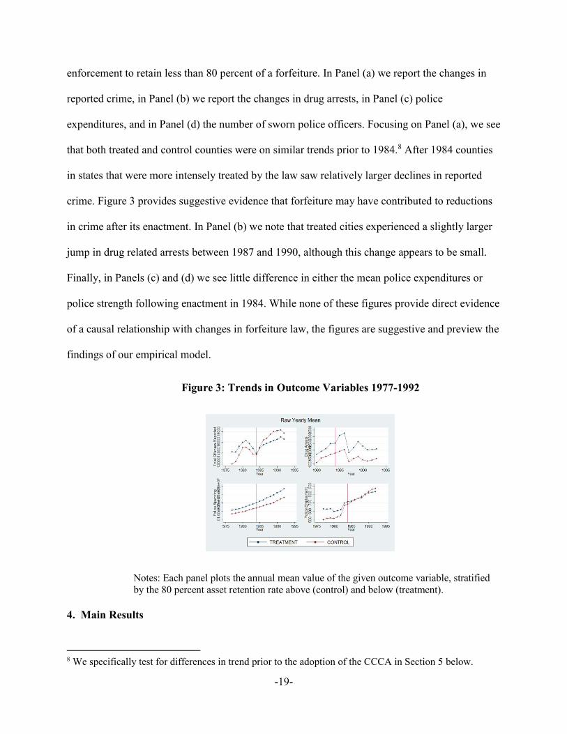
Before turning to the formal results, it is useful to inspect some of the trends in our main

outcome variables. In Figure 3 we report the mean dependent variable, stratified by control and

treatment based on the existing laws in 1983. Counties labeled as controls are located in states

that allowed law enforcement to retain more than 80 percent of the proceeds from forfeiture prior

to 1984, while counties labeled as treated are located in states that initially permitted law

7 Value of seizures inflated to 2016 dollars.

-19-

enforcement to retain less than 80 percent of a forfeiture. In Panel (a) we report the changes in

reported crime, in Panel (b) we report the changes in drug arrests, in Panel (c) police

expenditures, and in Panel (d) the number of sworn police officers. Focusing on Panel (a), we see

that both treated and control counties were on similar trends prior to 1984.8 After 1984 counties

in states that were more intensely treated by the law saw relatively larger declines in reported

crime. Figure 3 provides suggestive evidence that forfeiture may have contributed to reductions

in crime after its enactment. In Panel (b) we note that treated cities experienced a slightly larger

jump in drug related arrests between 1987 and 1990, although this change appears to be small.

Finally, in Panels (c) and (d) we see little difference in either the mean police expenditures or

police strength following enactment in 1984. While none of these figures provide direct evidence

of a causal relationship with changes in forfeiture law, the figures are suggestive and preview the

findings of our empirical model.

Figure 3: Trends in Outcome Variables 1977-1992

Notes: Each panel plots the annual mean value of the given outcome variable, stratified by the 80 percent asset retention rate above (control) and below (treatment).

4. Main Results

8 We specifically test for differences in trend prior to the adoption of the CCCA in Section 5 below.

-20-

4.1 Average Effect

We begin by presenting the results from estimation equation (1) using the reported crime

data. We present the results in Table 1, Panel A and report the coefficient from the

(1 − 𝐾𝑒𝑒𝑝𝑠,1984) × 1(𝑡 > 1984) interaction, with standard errors clustered at the county level

presented in parentheses. Panel A presents the unweighted results, although we will discuss the

impact of weighting by population later (Panel B). Each column of the table reports a different

level of crime data aggregation (i.e., total, violent, non-violent, and various sub-categories of

crimes). Following the intuition of the Becker (1968) model, we expect crime to fall as the

returns to such activity are reduced with the increased risk of forfeiture.

In Column (1) we report the impact of forfeiture on total reported crime. In states where

federal forfeiture was more generous than existing state law, we find that crime fell by an

average of 2,691 crimes. Evaluated at the mean number of crimes in the sample, increasing

police agencies’ ability to retain 80-90 percent of forfeited assets led to a 17.3 percent drop in

crime. Not surprisingly, the overall decrease in reported crime is associated with changes in non-

violent or property crime. In Columns (2) and (3), we report the estimates for violent and non-

violent crime separately. This finding is consistent with the notion that criminals are more likely

to respond to financial incentives when the crime is not an act of passion. In Columns (4) and (5)

we separately report the estimates for burglary and larceny which comprise over 90 percent of all

non-violent crimes (FBI, 2010). Within non-violent crime we estimate that about 58 percent of

the decline in total crime reported is driven by decreases in larceny. About 38 percent of the

reduction in non-violent crime is due to a decrease in burglary.

In Table 1, Panel B we report the estimates of forfeiture on the offenses reported, but

weight each observation by population. We do this to highlight the difference between the

-21-

impacts of forfeiture for the average citizen versus the average county. When we weight by

population, our estimates generally increase in absolute magnitude, however the relative

magnitude is slightly smaller (10.1 percent decrease in crime). The difference in magnitudes

suggests that the impact of expanded forfeiture powers are heterogeneous across counties (Solon,

Haider, and Wooldridge, 2015). We explore this and other sources of heterogeneity in Section 5

below.

Next, we consider police departments’ responses to the financial incentives of expanded

forfeiture opportunities. We expect that a profit-maximizing police chief would reallocate effort,

as measured by arrests, toward more profitable crimes. In Table 2 we report the reduced form

change in the number of total arrests, violent and non-violent crime arrests, as well as the change

in arrests for specific Index I crimes. Overall, we find that the total number of arrests in the

treatment states increased after 1984, however, the estimates are imprecise. If police respond to

financial incentives, we would expect the number of drug arrests to increase. While we estimate

a positive coefficient, it is imprecise over the entire post-1984 period. If police departments were

slow to respond to the financial incentives, then it is possible that the delay could push the entire

post-1984 estimate towards zero. In the next section we estimate the year-by-year effects of the

change in policy.

Finally, we consider whether local governments respond to increased forfeiture activity

by cutting budgets and by investing in additional police strength. Given the nature of Census

reporting, we are only able to measure total police expenditures, regardless of the funding

source. Thus, as long as local governments do not completely offset police budgets by the value

of seizures, we should estimate a non-decreasing relationship between expenditures and

forfeiture. In Table 3, Columns (1) and (3), we report the estimated relationship between

-22-

forfeiture and police expenditures. We estimate a positive relationship, however the magnitude is

generally small and not statistically significant at traditional levels. Broadly, our estimates

correspond to Baicker and Jacobsen (2007) who find that municipalities only partially reduce

appropriations in response to abnormally large seizures. We also report the estimated

relationship between the forfeiture and the size of the police force, measured by the number or

sworn officers. Should the police departments experience a budgetary bonanza, we might expect

that they respond by hiring additional officers. Our estimates, reported in Table 3, Columns (2)

and (4), do not support this notion, consistent with stable budgets. We do not find any evidence

of local law enforcement expanding faster in states more heavily influenced by the CCCA.

However, it is possible that our estimated decline in manpower could be the result of officers

diverted to new drug task forces, which were reported as separate agencies once they were

created. Unfortunately, data on the task forces’ manpower is ill-reported, so it is challenging to

empirically examine this conjecture. Alternatively, the reduction in officer numbers could be

driven by demand, as crime fell in the treated states relative to the controls.

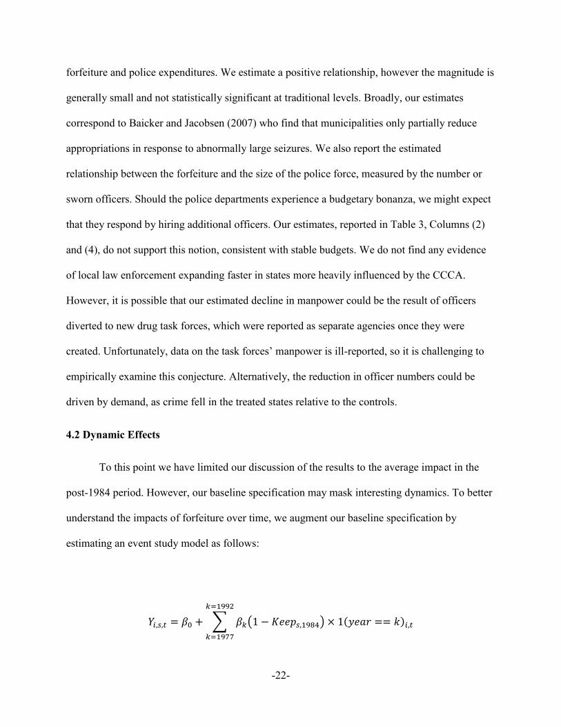
4.2 Dynamic Effects

To this point we have limited our discussion of the results to the average impact in the

post-1984 period. However, our baseline specification may mask interesting dynamics. To better

understand the impacts of forfeiture over time, we augment our baseline specification by

estimating an event study model as follows:

𝑌𝑖,𝑠,𝑡 = 𝛽0 + ∑ 𝛽𝑘(1 − 𝐾𝑒𝑒𝑝𝑠,1984) × 1(𝑦𝑒𝑎𝑟 == 𝑘)𝑖,𝑡

𝑘=1992

𝑘=1977

-23-

+𝛾𝑡𝑋𝑖,1970 + 𝛿𝑋𝑖,𝑡 + 𝜃𝑖 + 𝜇𝑡 + 휀𝑖,𝑡. (2)

This specification allows equitable sharing to have a different impact in each year of the sample

(relative to 1983). The event study specification also serves as a check on the validity of our

empirical strategy, as the CCCA should have no differential impact on outcomes in the years

prior to its enactment in 1984.

In Table 4 we report our year-by-year estimates for offenses reported (total crime, violent

crime, non-violent crime, burglary, and larceny). For brevity, we focus on total crime (Column

1) and non-violent crime (Column 3). First, note that the coefficients prior to the enactment of

the CCCA between 1977 and 1982. In each year we generally cannot reject that the coefficient is

zero.9 This result provides additional evidence that states with differing state forfeiture statutes

before 1984 were on similar trends just prior to the CCCA. After the change in forfeiture law, we

estimate a decrease in total and non-violent crimes through 1992, although the magnitude

declines beginning in the 1990s. The magnitudes are largest between 1986 and 1990. Why might

the reported crime rates initially dip and then return to the steady state? As noted earlier,

dynamic behavioral models of crime suggest that criminals update their information with

experience. If criminals believe that police will aggressively pursue forfeiture, then we should

estimate a large initial drop, especially after police departments have sufficient time to reallocate

their effort. If criminals learn over time that their priors overweight the probability of forfeiture,

then future decisions to commit a crime should account for these updated beliefs, perhaps

resulting in more crime later.

9 In 1977 there appear to be meaningful differences for all classes of crime except violent crime. However, in the years immediately before the enactment of equitable sharing, 1980-1982, there are no statistically significant differences for any crime outcome.

-24-

In Table 5 we report our time-varying estimates for the arrest outcomes. As before, we

report the estimates for total arrests, violent, non-violent, and drug crimes. Prior to the enactment

of the CCCA in 1984 we cannot reject that the estimate is zero. The lack of a statistically

significant difference in arrest outcomes in the pre-treatment period is reassuring and reinforces

the baseline empirical design that assumes states with different forfeiture policy prior to the

CCCA were on the same pre-trends. In the post-1984 period, we find little evidence that either

the total number or arrests, or arrests for violent and non-violent crimes changed. However, we

find that there is a large and statistically significant increase in the number of arrests for drug

crimes beginning in 1988. Between 1988 and 1992, the average increase in the number of drug

arrests is 732.9 per jurisdiction-year. Given that the average county had 1,951 drug arrests

annually, our estimates suggest that drug arrests increased by approximately 37.5 percent after

1988. The sizable increases in drug arrests suggest that police departments were responding to

the financial incentives that equitable sharing introduced. One open question is why the effect

took three to four years to appear. We believe that institutional frictions can help to explain the

delayed response. It took time for police departments to establish special drug task forces to take

advantage of the new federal law. Evidence of this policy lag can be seen in police surveys

themselves. The Law Enforcement Management and Administrative Statistics (LEMAS) survey

administered by the Bureau of Justice Statistics did not initially ask local law enforcement

agencies about the existence of special drug task forces. However, beginning in the 1990 version

of the survey, the agency began inquiring about such task forces and asset forfeitures. The

updated survey design provides anecdotal evidence that the widespread creation of such

specialized units was not immediate.

-25-

In Table 6 we report the year-by-year estimates using police expenditures and the number

of sworn officers as the outcomes of interest. Between 1978 and 1980, there is a difference in

expenditures, with less generous forfeiture states (i.e., the treatment states) providing lower rates

of funding. Yet in the years just prior to the enactment of the CCCA, spending across

jurisdictions in the different types of states was similar. For the post-1984 period, we find that

police expenditures are generally increasing over time, however, the estimates are imprecise. In

1984 and 1985, the coefficient is positive and statistically significant, with a magnitude

suggesting that police expenditures increased by 4.8 to 8.4 percent. While imprecise, this

evidence suggests that local governments were, at the very least, not taking away resources from

police faster than local law enforcement could seize revenue. Quickly, though, it seems that local

governments better understood the new source of revenue generated from seizures and budgets

adjusted accordingly.

In Table 6 Column (2) we report the year-by-year effect on sworn officer strength. Prior

to 1984, there were no significant differences between jurisdictions in different types of

forfeiture states. After the rollout of the CCCA, however, we estimate that police officer strength

declined by 32 to 97 officers, or between 4.5 and 13.9 percent relative to the mean, in states that

saw the largest incentive shock from the federal law. What might explain this relative decline in

officer strength? We partially attribute the decline to the formation of new gang and drug related

task forces. Overall, officer strength increased over time, as highlighted in Figure 3, however, the

formation of new drug task forces in existing jurisdictions could have siphoned officers from

existing units. As evidence of the siphoning effect, consider data from the 2007 Census of Law

-26-

Enforcement Gang Units. Of the 537 agencies in the Census, 89 had a gang unit as of 1992.10 Of

those 89, 73 were created between 1985 and 1992. The expansion of special units coincides with

the enactment of the CCCA and provides anecdotal evidence that our findings may be partially

explained by the changes in the composition of police units.

To recap, we find evidence that following the enactment of the federal equitable sharing

provision, reported crime, driven by non-violent property crimes, declined by approximately 17

percent, while drug arrests increased up to 37 percent, albeit after an initial delay following

enactment of the CCCA. Combined, these estimates suggest that civil asset forfeiture can be an

effective tool against certain types of crime, but may also incentivize police departments to

reallocate effort toward revenue-generating activities that may lead to its own unintended

consequences. We take up this idea in Section 5.6 below.

5. Robustness and Validity

To better understand our findings we conduct several robustness and validity exercises. We

begin by providing additional evidence that localities in each type of forfeiture state followed

similar trends prior to the enactment of the CCCA. There is also a potential concern that the time

period that we study is unique. The 1980s encompassed the crack epidemic in the United States,

so one might question whether the time fixed effects fully account for the intensity of the crack

boom across time and space? To address this concern, we estimate a set of placebo regressions

using crime data from Canada, which never adopted forfeiture statutes during our sample period,

but experienced similar trends in drug use.11

10 The 2007 Census of Law Enforcement Gang Units sampled police agencies with at least 100 sworn officers and at least 1 full time officer allocated to gangs. 11 The first civil asset forfeiture statute adopted in Canada was enacted in Ontario in 2001.

-27-

As noted above, the CCCA was a broad piece of crime-fighting legislation. Even though we

compare changes in outcomes between locations based on pre-existing differences in state

forfeiture law, these pre-existing laws might be correlated with other factors related to attitudes

toward crime or historic episodes, which were altered by the CCCA. Thus, we may not be

estimating the impact of forfeiture, but a composite effect of many provisions contained within

the CCCA. To address these concerns we consider specifications where we control for additional

variables related to a state’s position on crime prior to the federal law and historic measures of

racial tension. Next, in our presentation of our baseline results we highlighted the potential for

heterogeneity. Thus, we explore how our results differ according to county characteristics, such

as population and racial composition. Additionally, the quality of reported crime data is a

concern. To test whether crime or reported crime is changing in response to the CCCA, we

collect various measures of property value and test whether they respond to the enactment of

equitable sharing. Finally, we provide corroborating evidence that police may reallocate effort

toward more profitable drug enforcement by examining changes in traffic fatalities.

5.1 Parallel Trends

Our baseline strategy implicitly assumes that states with both generous and stingy pre-

existing forfeiture statutes followed similar time paths prior to the enactment of the CCCA.

Previously, we noted that the year-by-year coefficients were generally zero in pre-treatment

years. To further test the validity of the parallel trends assumption, we restrict the sample to the

period prior to the enactment of the CCCA and specify the following regression:

𝑌𝑖,𝑠,𝑡 = 𝛽0 + 𝛽1𝑇𝑟𝑒𝑎𝑡𝑖,𝑠 + 𝛽2𝑡 + 𝛽3𝑇𝑟𝑒𝑎𝑡𝑖,𝑠 × 𝑡 + 𝛾𝑡𝑋𝑖,1970 + 𝛿𝑋𝑖,𝑡 + 𝜇𝑡 + 휀𝑖,𝑡. (3)

-28-

In this regression we define 𝑇𝑟𝑒𝑎𝑡𝑖,𝑠 as any county in a state that permitted local law

enforcement to retain less than 80 percent of the proceeds from a forfeiture and 𝑡 is a linear time

trend. The coefficient 𝛽3 tests whether jurisdictions that eventually benefitted from the

enactment of forfeiture are on a different time trend than the control counties.

Our results from this exercise are reported in Table 7. In Panel A we report the estimates

of 𝛽3 for the outcomes related to reported offenses. In Panel B we report the outcomes related to

arrests. Across all outcomes we cannot reject that both types of counties/jurisdictions followed

the same time trends prior to CCCA enactment, lending additional support to our empirical

design.

5.2 Canadian Placebo

Our primary dataset encompasses a unique period in the United States. In terms of

macroeconomic conditions, the country exited a recession in the early 1980s, experienced

growth, and then entered another mild recession at the end of the Bush Administration. The

nation also suffered from a severe drug epidemic related to crack cocaine. Given these changes

one might question whether year fixed effects fully absorb these changes in macroeconomic

conditions. To mitigate concerns that our baseline estimates are the result of a spurious

correlation, we specify a set of placebo regressions using crime data from Canada. Canada is

uniquely suited to test the robustness of our main findings. Macro conditions throughout the

1980s and the experience with the drug epidemic were similar in Canada, yet Canada nor its

provinces had instituted a law enabling forfeiture during our sample period. Canada also collects

Uniform Crime Reports for a variety of criminal offenses from its police jurisdictions. If our

main findings are the result of the enactment of the CCCA and not the result of a spurious

-29-

correlation, we should not find any effect of the equitable sharing rule in the Canadian sample.

To operationalize this falsification experiment we randomly assign a placebo province-level

retention rate for seized property that matches the observed distribution in the United States. This

random assignment ensures that at least one province always begins with a retention rate of 100

percent, while the majority of provinces have rates set below 80 percent, which mimics the U.S.

case. We then substitute these rates into Equation (1) and estimate the equation. In total, we

specify 15 permutations of these placebo retention rates at the province level.

We present our 15 sets of estimates for total crime, violent crime, and non-violent crime

in Table 8. Each coefficient in the table is the estimate from a separate regression. Each row

refers to a specific permutation of the placebo retention rates, while each column refers to a

separate outcome using that permutation. As expected, almost all of our estimates are statistically

insignificant, and are distributed about zero. This finding lends credence that our baseline

specification is not the result of a spurious correlation, but instead captures the impact of the U.S.

policy change.

5.3 Changes in Attitude Toward Crime

The CCCA was a broad piece of legislation that expanded police powers, altered rules for

establishing bail, facilitated federal sentencing reform, and possibly changed local attitudes

toward crime. If the federal government, through the enactment of the CCCA, pressured states to

become tougher on crime, then our estimates may reflect the bundle of changes associated with

the CCCA that extend beyond forfeiture. To address this concern we add additional covariates to

our main regression to capture pre-existing differences across states in their enforcement and

attitudes toward crime. First, we include a measure of the per capita incarceration rate at the state

level in 1981, drawn from the DOJ’s Sourcebook of Criminal Justice Statistics, and interact it

-30-

with year fixed effects. By controlling for the pre-existing state-level incarceration rates, we

allow states that were initially tough or soft on crime to evolve differently over time. Second, as

the War on Drugs expanded, it may have altered the distribution of cases and effort across

federal and state/local agencies across the country. To address this concern, we measure the

share of federal defendants who originated from each state prior to the enactment of the CCCA

(again, drawing data from the DOJ’s Sourcebook of Criminal Justice Statistics). Our intent is to

proxy for the pre-existing intensity of federal prosecution in a given location, as locations with

initially high levels of federal prosecution may evolve differently than those where the federal

government was initially less active. Finally, during the 1960s and early 1970s, many

communities experienced race riots. The experiences in these communities during the 1960s

could have persistent effects with regards to the interaction with police forces and future policies

that altered police power. To control for this possible race riot channel, we add a control for the

number of race riots in each county during the 1960s, drawing on data from Carter (1986) and

Collins and Margo (2007).

In Table 9, we report estimates of Equation (1) using reported crime as the outcome of

interest. In column (1) we display our baseline estimates (replicated from Table 1), while

columns (2) - (4) report the additional estimates. When we include the initial incarceration rate

per capita, the share of federal cases originating in each state, or the intensity of race riots during

the 1960s, our estimates remain qualitatively similar. Indeed, each point estimate with the

additional controls lies within the confidence interval of the baseline estimates. Given the

similarity of the estimates after the inclusion of the additional controls, it is more likely that the

estimates are the result of equitable sharing and not changes in attitudes towards crime that may

have accompanied the CCCA.

-31-

5.4 Heterogeneity

To further investigate the impact of county population and the size of minority populations,

we augment Equation (1) by interacting either population or the percent black with the main

treatment variables. In Table 10 we report our estimates for the total level of reported crime,

violent crime, non-violent crime, burglary, and larceny. Our estimates suggest the presence of

heterogeneity based on population. For burglary and larceny, which account for approximately

90 percent of all crimes, we estimate that increases in population result in fewer crimes. Based

on our estimates an increase in population from the sample mean to a county population of

500,000 would result in an additional decrease of 813 burglaries (21 percent relative to the mean)

and 308 larcenies (3.6 percent relative to the mean).

Given the potential for police departments to discriminate against minorities, we might

expect larger declines in crime in places where minority groups are concentrated, especially if

minorities view the penalties as more likely or more severe (Mustard, 2001; Donohue and Levitt,

2001b; Antonovics and Knight, 2009; Price and Wolfers, 2010; Abrams et al., 2012; Rehavi and

Starr, 2014; Horrace and Rohlin, 2016). We generally estimate negative coefficients on the

interaction term between race and treatment, suggesting larger declines in burglaries in locations

with relatively larger minority populations. These estimates might be perceived as evidence of

potential discrimination in the use of forfeiture, yet in most instances the estimates lack statistical

precision, making such strong conclusions difficult to support empirically.

5.5 Property Values

Using reported crime as a proxy for the true crime conditions in a location could raise

concern. Changes in reporting may itself be a function of expanded forfeiture activity.

-32-

Individuals who were victimized may perceive that their property is at risk if they report a crime,

or the policy may generally generate ill will towards the police, especially in light of the

potential for the abuse of civil liberties. Therefore, it is not clear that our estimates reflect

changes in reporting or real changes in crime. To address this we replace the outcome in

Equation (1) with either the decennial Census’s median home value for the decades 1970-1990,

or use the state-level quarterly price index reported by the Federal Housing Financing Agency

(FHFA) for the period 1977-1992.12 This strategy relies on the existing literature that has

documented the relationship between property values and crime (Lynch and Rasmussen, 2004;

Collins and Margo, 2007; Tracey and Rockoff, 2008; Pope and Pope, 2012, Ajzenman, Galiani,

Seira, 2015; Cunningham, 2016). If reporting responds to forfeiture, while the actual level of

crime remains fixed, property values should not respond to the enactment of the law. Conversely,

if crime (and not just reporting) declines in response increased forfeiture activity, we should

estimate a positive relationship between forfeiture and property values.

Indeed, in Table 11 we report that both the median home values measured by the Census and

the FHFA price index both increase in places more strongly treated after the enactment of the

CCCA. In Column (2) we find that home values increase by 1.67 percent for a 10 percent

increase in assets retained by local law enforcement. Using the FHFA measure we estimate

slightly larger magnitudes. Combined, these different measures of property values suggest that

the actual level of crime was decreasing, rather than just changes in reporting behavior.

5.6 Reallocation of Police Effort

12 The FHFA also constructs a price index at the MSA level, however, only 39 MSAs began reporting on or before 1977 that fall within our 38 state sample. The results using the quarterly MSA data are qualitatively similar to our estimates at the state level.

-33-

Police departments have relatively few mechanisms to generate revenue. One key source of

revenue over time has been traffic citations. Indeed, traffic ticket revenues often fund portions of

police salaries and citations are sensitive to local fiscal conditions (Markowsky and Stratmann,

2009; Garrett and Wagner, 2009). If forfeiture becomes a new tool to generate revenue, with a

potentially higher marginal revenue than routine traffic stops, profit maximization suggests that

police departments would reallocate effort from traffic enforcement to policing drug crime. The

economics literature has found that drivers are responsive to changes in enforcement on roads

and highways. In Oregon, for example, following a severe budget cut in 2003, state highway

patrols were cut by 35 percent, resulting in a 10-20 percent increase in auto-related injuries and

fatalities (DeAngelo and Hansen, 2014). Similarly, there is evidence that increased traffic

monitoring during campaigns such as Click-it-or-Ticket also reduces motor vehicle fatalities

(Luca, 2015). Traffic citations also respond to budget shocks, which leads to increased road

safety (Makowsky and Stratmann, 2011).

To indirectly test whether police reallocated effort away from traffic enforcement to other

revenue-generating activities, we follow DeAngelo and Hansen (2014) and estimate a Poisson

regression as follows:

𝐸(𝑑𝑒𝑎𝑡ℎ𝑠𝑖𝑠𝑡) = exp[𝛽0 + 𝛽1(1 − 𝐾𝑒𝑒𝑝𝑠,1984) × 1(𝑡 ≥ 1984) + 𝛾𝑉𝑀𝑇𝑠𝑡 + 𝜃𝑖 + 𝜇𝑡] (4).

The dependent variable is either the number of people in fatal accidents or the number of

vehicular fatalities in a given county-year. The fatality and accident data are compiled from the

microdata reported by the National Highway Traffic Safety Administration’s (NHTSA) Fatality

Analysis Reporting System (FARS) Accident series for the period 1977-1992. Unlike DeAngelo

and Hansen (2014), who used state-level data, we do not explicitly scale for vehicle miles

traveled because they are not reported at the county level. Instead, we control for the annual

-34-

state-level VMT that we collected from yearly volumes of the Federal Highway Administration’s

“Highway Statistics” report. Controlling for VMT, rather than scaling by VMT does not force

the coefficient 𝛾 to be equal to 1. We also control for county fixed effects and year fixed effects.

In Table 12 we report the estimated deadly accident and fatality elasticities associated

with the enactment of the CCCA for two samples. The first sample consists of all counties in the

38 states for which we have coded forfeiture statutes. Our second sub-sample is constructed to

match the counties in our reported crime sample. Because we impose a population cutoff of

50,000 to appear in the crime samples, the accident and fatality sub-sample consists of counties

that are more populous and urbanized relative to the full sample of counties. In Column (1), we

report the elasticity for the number of people involved in a fatal crash, while in Column (2) we

report the elasticity with respect to fatalities using the full sample. In Columns (3) and (4) we

report the analogous estimates using the restricted (more urban) sample. Focusing on the

elasticity with respect to fatalities (Column (2)), we estimate that for a 10 percent increase in

forfeited assets retained, traffic fatalities increase by 2.8 percent. In the restricted sample, the

estimate is similar, a 10 percent increase in forfeited assets retained leads to a 2.3 percent

increase in fatalities. Provided that many states in our sample experienced an 80 percent increase

in local proceeds from forfeiture, we estimate that fatalities in the treated states increased by

18.4-22.7 percent relative to untreated states. These estimates are similar in magnitude to the

estimates reported in DeAngelo and Hansen (2014).

Given the mean number of fatalities in each sample, the estimates imply that treated

counties experience anywhere from 3.2-7.75 additional traffic fatalities per year. As of 2016, the

U.S. Department of Transportation (USDOT) assesses a value of a statistical life at $9.6 million.

Applying the USDOT’s valuation to our estimates suggests that there is a hidden cost of $30.7-

-35-

$74.4 million associated with the enforcement of the CCCA.13 This finding suggests that there

are potentially large externality costs associated with the implementation of civil asset forfeiture

that have not previously been documented in the literature. While this finding is not direct

evidence that police reduced their traffic patrols in response to the enactment of equitable

sharing, it is suggestive that such a reallocation occurred and has led to a significant unintended

consequence of the law.

6. Conclusions

Civil asset forfeiture was initially proposed as a means to “cut the head off the snake” and to

limit the gains that criminal organizations obtained through their illicit activities. Lawmakers

hoped that by reducing the financial returns from crime, crime would be reduced. The financial

incentives created within the forfeiture environment, however, have the potential to alter police

incentives. Indeed, these incentives are strong enough to have raised significant civil liberties

concerns. Recently, over concerns of abuse and the potential violation of habeas corpus, the

Department of Justice suspended federal civil asset forfeiture in the absence of a criminal charge

or warrant. Several states have also begun to reform their approach to forfeiture, either by

increasing the standard of proof or requiring that a forfeiture be accompanied by a criminal

conviction. Understanding the impacts of civil asset forfeiture is especially important as

legislators debate its reform. There is currently an open question regarding the distributional

impacts of forfeiture and whether specific groups have been targeted by police. Recent forfeiture

level data from Chicago indicate that forfeitures are overwhelmingly carried out in low income

and minority communities; and while forfeiture is intended to target kingpins, the median seizure

13 https://www.transportation.gov/sites/dot.gov/files/docs/2016%20Revised%20Value%20of%20a%20Statistical%20Life%20Guidance.pdf

-36-

has totaled just over $1,000 (often in cash), which has led some to challenge police practices

with regard to forfeiture.14 The recent spotlight that has been shining on forfeiture as a crime-

fighting tool makes it increasingly important to understand how the system affects the behavior

of participants in the criminal justice system and generates intended and unintended

consequences.

We estimate that between 1984 and 1992 changes in forfeiture opportunities contained in

the CCCA led to a 17 percent reduction in non-violent property crimes in places where police

could suddenly keep a larger share of their seizures. The bulk of this reduction is driven by

changes in burglary and larceny. Thus, reducing the financial incentives of crime through

equitable sharing seems to have achieved one of the primary objectives of forfeiture – that is, to

reduce crime. The altered financial incentives that police departments faced as a result of the

CCCA led them to reallocate effort toward fighting drug crimes, where the opportunity to seize

cash was greatest. We estimate that between 1989 and 1992, drug arrests increased by

approximately 37 percent in the treated states. We also find suggestive evidence that police were

reallocating effort away from traffic enforcement and toward drug crime. We estimate that

traffic fatalities increased by about 22 percent after the enactment of equitable sharing. While our

analysis reveals that civil asset forfeiture may help to achieve some of the policy goals that

proponents tout, it also raises new concerns about the unintended negative consequences of the

law, beyond the civil liberties concerns that opponents emphasize.

14 http://www.chicagotribune.com/news/opinion/commentary/ct-chicago-civil-asset-forfeiture-20170614-story.html

-37-

References

Abrams, D.., Bertrand, M. and Mullainathan, S. "Do Judges Vary in Their Treatment of Race?." The Journal of Legal Studies 41, no. 2 (2012): 347-383.

Aisch, Gregor and Alicia Parplpiano. “What do you Think is the Most Important Problem Facing this Country Today?.” New York Times. Feb. 27, 2017. Accessed August 17, 2017. https://www.nytimes.com/interactive/2017/02/27/us/politics/most-important-problem-gallup-polling question.html?hp&action=click&pgtype=Homepage&clickSource=g-artboard%20g-artboard-v3%20&module=b-lede-package-region&region=top-news&WT.nav=top-news

Ajzenman, Nicolas, Sebastian Galiani, and Enrique Seira. "On the distributive costs of drug-related homicides." The Journal of Law and Economics 58, no. 4 (2015): 779-803.

Antonovics, K., and Knight, B. "A new look at racial profiling: Evidence from the Boston Police Department." The Review of Economics and Statistics 91, no. 1 (2009): 163-177.

Baicker, K., and Jacobson, M.. "Finders keepers: Forfeiture laws, policing incentives, and local budgets." Journal of Public Economics 91.11 (2007): 2113-2136.

Becker, G. "Crime and Punishment: An Economic Approach." Journal of Political Economy 76, no. 2 (1968): 169-217.

Benson, B., Rasmussen, D. and Sollars, D. "Police bureaucracies, their incentives, and the war on drugs." Public Choice 83, no. 1 (1995): 21-45.

Boudreaux, D., and Pritchard, A. "Civil forfeiture and the war on drugs: Lessons from economics and history." San Diego L. Rev. 33 (1996): 79.

Carpenter, D. Knepper, L., Erickson, A., and McDonald, J. "Policing for profit: the abuse of civil asset forfeiture." Institute for Justice 2 (2015).

Carter, Gregg Lee. "The 1960s black riots revisited: city level explanations of their severity." Sociological Inquiry 56, no. 2 (1986): 210-228.

Chalfin, Aaron, and Justin McCrary. "Criminal deterrence: A review of the literature." Journal of

Economic Literature 55, no. 1 (2017): 5-48.

Collins, William J., and Robert A. Margo. "The economic aftermath of the 1960s riots in American cities: Evidence from property values." The Journal of Economic History 67, no. 4 (2007): 849-883.

Cunningham, Jamein P. "An evaluation of the Federal Legal Services Program: Evidence from crime rates and property values." Journal of Urban Economics 92 (2016): 76-90.

DeAngelo, Gregory, and Benjamin Hansen. "Life and death in the fast lane: Police enforcement and traffic fatalities." American Economic Journal: Economic Policy 6, no. 2 (2014): 231-257.

-38-

Donohue III, John J., and Steven D. Levitt. "The impact of legalized abortion on crime." The

Quarterly Journal of Economics 116, no. 2 (2001): 379-420.

Donohue, John J., and Steven D. Levitt. "The impact of race on policing and arrests." The

Journal of Law and Economics 44, no. 2 (2001): 367-394.

Garrett, Thomas A., and Gary A. Wagner. "Red ink in the rearview mirror: Local fiscal conditions and the issuance of traffic tickets." The Journal of Law and Economics 52, no. 1 (2009): 71-90.

Handley, Joel, and Freddy Martinez. “Inside the Chicago Police Department’s secret budget.” Chicago Reader. September 29, 2016. Accessed August 14, 2017. https://www.chicagoreader.com/chicago/police-department-civil-forfeiture-investigation/Content?oid=23728922

Haines, Michael R. "Historical, Demographic, Economic, and Social Data: The United States, 1790-2002 [Computer file]. ICPSR02896-v3. Inter-university Consortium for Political and Social Research." Ann Arbor, MI (2010).

Holcomb, Jefferson E., Tomislav V. Kovandzic, and Marian R. Williams. "Civil asset forfeiture, equitable sharing, and policing for profit in the United States." Journal of Criminal Justice 39, no. 3 (2011): 273-285.

Horrace, William C., and Shawn M. Rohlin. "How dark is dark? Bright lights, big city, racial profiling." Review of Economics and Statistics 98, no. 2 (2016): 226-232.

Kelly, Brian D., and Maureen Kole. "The effects of asset forfeiture on policing: a panel approach." Economic Inquiry 54, no. 1 (2016): 558-575.

Levitt, Steven D. "The effect of prison population size on crime rates: Evidence from prison overcrowding litigation." The quarterly journal of economics 111, no. 2 (1996): 319-351.

Levitt, Steven D. "The relationship between crime reporting and police: Implications for the use of Uniform Crime Reports." Journal of Quantitative Criminology 14, no. 1 (1998): 61-81.

Levitt, Steven D. "The limited role of changing age structure in explaining aggregate crime rates." Criminology 37, no. 3 (1999): 581-598.

Levitt, Steven D. "Understanding why crime fell in the 1990s: Four factors that explain the decline and six that do not." The Journal of Economic Perspectives 18, no. 1 (2004): 163-190.

Luca, Dara Lee. "Do traffic tickets reduce motor vehicle accidents? Evidence from a natural experiment." Journal of Policy Analysis and Management 34, no. 1 (2015): 85-106.

Lynch, Allen K., and David W. Rasmussen. "Proximity, neighborhood and the efficacy of exclusion." Urban Studies 41, no. 2 (2004): 285-298.

Makowsky, Michael D., and Thomas Stratmann. "Political economy at any speed: what determines traffic citations?." The American Economic Review 99, no. 1 (2009): 509-527.

-39-

Makowsky, Michael D., and Thomas Stratmann. "More tickets, fewer accidents: How cash-strapped towns make for safer roads." The Journal of Law and Economics 54, no. 4 (2011): 863-888.

Mas, Alexandre. "Pay, reference points, and police performance." The Quarterly Journal of

Economics 121, no. 3 (2006): 783-821.

Mast, Brent D., Bruce L. Benson, and David W. Rasmussen. "Entrepreneurial police and drug enforcement policy." Public Choice 104, no. 3-4 (2000): 285-308.

Mumola, Christopher J., and Jennifer C. Karberg. Drug use and dependence, state and federal

prisoners, 2004. Washington, DC: US Department of Justice, Office of Justice Programs, Bureau of Justice Statistics, 2006.

O’Harrow, Robert Jr., Sari Horwitz, and Steven Rich. "Attorney General Holder limits civil seizure process that split billions of dollars with local and state police." The Washington Post. January 16, 2015. Accessed August 14, 2017. https://www.washingtonpost.com/investigations/holder-ends-seized-asset-sharing-process-that-split-billions-with-local-state-police/2015/01/16/0e7ca058-99d4-11e4-bcfb-059ec7a93ddc_story.html?utm_term=.a8ac790b41d6.

Pope, Devin G., and Jaren C. Pope. "Crime and property values: Evidence from the 1990s crime drop." Regional Science and Urban Economics 42, no. 1 (2012): 177-188.

Price, Joseph, and Justin Wolfers. "Racial Discrimination Among NBA." The Quarterly Journal

of Economics (2010): 1859-1887.

Rehavi, M. Marit, and Sonja B. Starr. "Racial disparity in federal criminal sentences." Journal of

Political Economy 122, no. 6 (2014): 1320-1354.

Schwarcz, Steven L., and Alan E. Rothman. "Civil Foreiture: A Higher Form of Commerical Law." Fordham L. Rev. 62 (1993): 287.

Shi, Lan. "The limit of oversight in policing: Evidence from the 2001 Cincinnati riot." Journal of

Public Economics 93, no. 1 (2009): 99-113.

Snead, Jason. "An Overview of Recent State-Level Forfeiture Reforms." The Heritage Foundation. August 23, 2016. Accessed August 14, 2017. http://www.heritage.org/crime-and-justice/report/overview-recent-state-level-forfeiture-reforms.

Solon, Gary, Steven J. Haider, and Jeffrey M. Wooldridge. "What are we weighting for?." Journal of Human resources 50, no. 2 (2015): 301-316.

Stellwagen, Lindsey D., and Kimberly A. Wylie. Strategies for supplementing the police budget. US Department of Justice, National Institute of Justice, Office of Development, Testing and Dissemination, 1985.

Tracey, D. and Rockoff, J.E., 2008. Estimates of the impact of crime risk on property values from Megan's laws. The American Economic Review, 98(3), pp.1103-1127.

-40-

Trott, Stephen S. "Implementing criminal justice reform." Public Administration Review (1985): 795-800.

United States Comptroller General, and United States of America. "Asset Forfeiture: A Seldom Used Tool in Combatting Drug Trafficking." (1981).

United States. Congress. House. Committee on the Judiciary. Civil Asset Forfeiture Reform Act:

report together with dissenting views (to accompany H.R. 1658) (including cost estimate of the

Congressional Budget Office). United States Government Printing Office. Washington, D.C. 1999.

United States. Congress. Senate. Committee on the Judiciary. Subcommittee on Criminal Justice. Forfeiture of narcotics proceeds: hearings before the Subcommittee on Criminal Justice

of the Committee on the Judiciary, United States Senate, Ninety-sixth Congress, second session,

on forfeiture of profits of narcotics traffickers, July 23 and 24, 1980. United States Government Printing Office. Washington, D.C. 1981.

United States Department of Justice, Federal Bureau of Investigation. Uniform Crime Reporting Program Data [United States]: County-Level Detailed Arrest and Offense Data, 1977-1993. Ann Arbor, MI: Inter-university Consortium for Political and Social Research [producer and distributor], 1977-1992. c

United States Department of Justice. Federal Bureau of Investigation. Uniform Crime Reporting Program Data [United States]: Arrests by Age, Sex, and Race, 1977-1992. ICPSR23344-v1. Ann Arbor, MI: Inter-university Consortium for Political and Social Research [distributor], 2009-03-06. http://doi.org/10.3886/ICPSR23344.v1

United States Department of Commerce, Bureau of the Census. ANNUAL SURVEY OF GOVERNMENTS: FINANCE STATISTICS. Washington, DC: U.S. Dept. of Commerce, Bureau of the Census [producer], 1977-1992. Ann Arbor, MI: Inter-university Consortium for Political and Social Research [distributor], 1984. http://doi.org/10.3886/ICPSR08146.v1

Worrall, John L. "Addicted to the drug war: The role of civil asset forfeiture as a budgetary necessity in contemporary law enforcement." Journal of Criminal Justice 29, no. 3 (2001): 171-187.

Worrall, John L., and Tomislav V. Kovandzic. "Is policing for profit? Answers from asset forfeiture." Criminology & Public Policy 7, no. 2 (2008): 219-244.

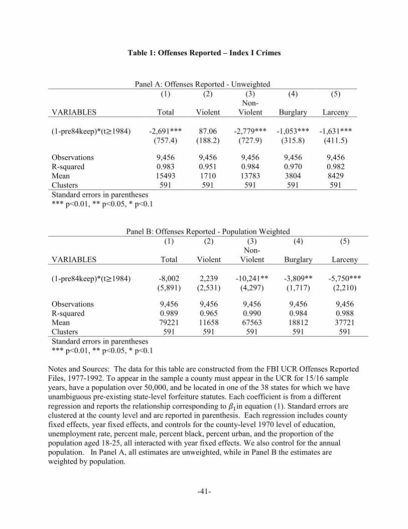
-41-

Table 1: Offenses Reported – Index I Crimes

Panel A: Offenses Reported - Unweighted (1) (2) (3) (4) (5)

VARIABLES Total Violent Non-

Violent Burglary Larceny

(1-pre84keep)*(t≥1984) -2,691*** 87.06 -2,779*** -1,053*** -1,631***(757.4) (188.2) (727.9) (315.8) (411.5)

Observations 9,456 9,456 9,456 9,456 9,456 R-squared 0.983 0.951 0.984 0.970 0.982 Mean 15493 1710 13783 3804 8429 Clusters 591 591 591 591 591 Standard errors in parentheses *** p<0.01, ** p<0.05, * p<0.1

Panel B: Offenses Reported - Population Weighted (1) (2) (3) (4) (5)

VARIABLES Total Violent Non-

Violent Burglary Larceny

(1-pre84keep)*(t≥1984) -8,002 2,239 -10,241** -3,809** -5,750***(5,891) (2,531) (4,297) (1,717) (2,210)

Observations 9,456 9,456 9,456 9,456 9,456 R-squared 0.989 0.965 0.990 0.984 0.988 Mean 79221 11658 67563 18812 37721 Clusters 591 591 591 591 591 Standard errors in parentheses *** p<0.01, ** p<0.05, * p<0.1

Notes and Sources: The data for this table are constructed from the FBI UCR Offenses Reported Files, 1977-1992. To appear in the sample a county must appear in the UCR for 15/16 sample years, have a population over 50,000, and be located in one of the 38 states for which we have unambiguous pre-existing state-level forfeiture statutes. Each coefficient is from a different regression and reports the relationship corresponding to 𝛽1in equation (1). Standard errors are clustered at the county level and are reported in parenthesis. Each regression includes county fixed effects, year fixed effects, and controls for the county-level 1970 level of education, unemployment rate, percent male, percent black, percent urban, and the proportion of the population aged 18-25, all interacted with year fixed effects. We also control for the annual population. In Panel A, all estimates are unweighted, while in Panel B the estimates are weighted by population.

-42-

Table 2: Arrests – Index I Crimes

Panel A: Arrests- Unweighted Estimates (1) (2) (3) (4) (5) (6) (7) (8) (9) (10)

VARIABLES Total ViolentNon-

Violent Drug Robbery Agg

Assault Oth

Assault Burglary Larceny Vehicular

(1-pre84keep)*( t≥1984) 598.2 -86.38 564.6 120.0 82.27 140.2** -255.4** 241.1 213.3 110.2 (705.8) (188.6) (655.7) (296.5) (121.5) (70.33) (112.2) (230.8) (376.3) (77.04)

Observations 2,431 2,431 2,431 2,431 2,431 2,431 2,371 2,431 2,431 2,431 R-squared 0.956 0.949 0.936 0.928 0.964 0.948 0.920 0.913 0.917 0.969 Mean 8170 2418 3801 1951 488.7 686.2 1275 865.5 2561 375.4 Clusters 187 187 187 187 187 187 187 187 187 187 Robust standard errors in parentheses *** p<0.01, ** p<0.05, * p<0.1

Panel B: Population Weighted Estimates (1) (2) (3) (4) (5) (6) (7) (8) (9) (10)

VARIABLES Total ViolentNon-

Violent Drug Robbery Agg

Assault Oth

Assault Burglary Larceny Vehicular

(1-pre84keep)*( t≥1984) 2,446 482.1 235.4 1,728 -292.2 1,035** 261.4 132.8 -545.9 648.6** (2,677) (422.8) (2,282) (1,377) (498.2) (453.3) (450.3) (690.7) (1,562) (316.8)

Observations 2,431 2,431 2,431 2,431 2,431 2,431 2,371 2,431 2,431 2,431 R-squared 0.987 0.984 0.978 0.983 0.994 0.986 0.948 0.978 0.966 0.991 Mean 66824 21329 24938 20557 6765 6620 8106 5858 15171 3909 Clusters 187 187 187 187 187 187 187 187 187 187 Robust standard errors in parentheses *** p<0.01, ** p<0.05, * p<0.1

-43-

Notes and Sources: The data for this table are constructed from the FBI UCR Arrests Files, 1980-1992. To appear in the sample a police jurisdiction must appear in the UCR for 12/13 sample years, have a population over 50,000, and be located in one of the 38 states for which we have unambiguous pre-existing state-level forfeiture statutes. Each coefficient is from a different regression and reports the relationship corresponding to 𝛽1in equation (1). Standard errors are clustered at the police jurisdiction level and are reported in parenthesis. Each regression includes police jurisdiction fixed effects, year fixed effects, and controls for the county-level 1970 level of education, unemployment rate, percent male, percent black, percent urban, and the proportion of the population aged 18-25, all interacted with year fixed effects. We also control for the annual population. In Panel A, all estimates are unweighted, while in Panel B the estimates are weighted by population.

-44-

Table 3: Police Expenditures and Sworn Officers

Police Expenditures and Sworn Officers Unweighted Weighted

(1) (2) (3) (4)

VARIABLES

Police Expenditures ($100,000)

Sworn Officers

Police Expenditures ($100,000)

Sworn Officers

(1-pre84keep)*( t ≥1984) 43.28 -82.50* 225.6 -366.2**(29.43) (47.26) (189.6) (162.0)

Observations 9,040 9,376 9,040 9,376 R-squared 0.936 0.982 0.974 0.994 Mean 196.2 698.5 1238 3491 Clusters 565 586 565 586 Standard errors in parentheses *** p<0.01, ** p<0.05, * p<0.1

Notes and Sources: Sworn Officer data is drawn from the FBI UCR LEOKA 1977-1992, while Police Expenditure data is from the Census of Government Finances, 1977-1992. To appear in the sample a county must appear in the UCR for 15/16 sample years, have a population over 50,000, and be located in one of the 38 states for which we have unambiguous pre-existing state-level forfeiture statutes. Each coefficient is from a different regression and reports the relationship corresponding to 𝛽1in equation (1). Standard errors are clustered at the county level and are reported in parenthesis. Each regression includes county fixed effects, year fixed effects, and controls for the county-level 1970 level of education, unemployment rate, percent male, percent black, percent urban, and the proportion of the population aged 18-25, all interacted with year fixed effects. We also control for the annual population. Columns (1) and (2) report the unweighted estimates, while Columns (3) and (4) report population weighted estimates.

-45-

Table 4: Offenses Reported: Dynamic Effect (Unweighted)

Offenses Reported- Dynamic Effects (1) (2) (3) (4) (5)

VARIABLES Total Violent Non-Violent Burglary Larceny

(1-pre84keep)*(t=1977) 1,190** -113.6 1,303*** 708.8*** 512.6** (502.9) (172.7) (432.3) (218.2) (254.0)

(1-pre84keep)*(t=1978) 893.7* -78.13 971.9** 675.0*** 210.0 (499.1) (149.1) (418.2) (202.5) (230.7)

(1-pre84keep)*(t=1979) 727.6 -46.21 773.8** 436.8** 261.4 (446.9) (118.1) (380.9) (169.6) (207.1)

(1-pre84keep)*(t=1980) 235.2 -169.4 404.6 304.6 159.0 (502.4) (143.3) (414.9) (218.0) (199.6)

(1-pre84keep)*(t=1981) -4.328 -28.26 23.93 -27.37 46.35 (425.6) (85.59) (377.4) (194.1) (253.2)

(1-pre84keep)*(t=1982) -17.78 -34.32 16.55 -75.74 91.12 (372.1) (67.28) (328.4) (153.6) (178.6)

(1-pre84keep)*(t=1983) 0 0 0 0 0

(1-pre84keep)*(t=1984) -1,500** -110.1 -1,390** -549.1** -633.7*(759.2) (120.3) (647.2) (227.5) (353.1)

(1-pre84keep)*(t=1985) -1,558*** -9.316 -1,549*** -546.1*** -879.1***(432.6) (74.61) (395.6) (157.9) (234.3)

(1-pre84keep)*(t=1986) -2,424*** -14.50 -2,409*** -942.2*** -1,343***(673.7) (118.8) (622.9) (241.4) (330.5)

(1-pre84keep)*(t=1987) -3,056*** 8.720 -3,065*** -1,137*** -1,809***(886.5) (119.1) (846.0) (312.1) (460.4)

(1-pre84keep)*(t=1988) -2,893*** 3.679 -2,897*** -1,078*** -1,760***(1,001) (144.8) (931.1) (342.3) (500.4)

(1-pre84keep)*(t=1989) -2,971*** 47.16 -3,018*** -1,058*** -1,858***(1,075) (192.1) (983.7) (351.8) (522.0)

(1-pre84keep)*(t=1990) -2,690*** -22.77 -2,667*** -836.8** -1,761***(970.1) (243.5) (871.4) (336.2) (483.6)

(1-pre84keep)*(t=1991) -1,930** 83.73 -2,014** -517.6* -1,542***(907.5) (281.4) (791.7) (312.9) (467.1)

(1-pre84keep)*(t=1992) -1,355* 194.1 -1,549** -234.3 -1,471***(743.9) (251.5) (708.4) (339.2) (413.7)

Observations 9,456 9,456 9,456 9,456 9,456 R-squared 0.983 0.951 0.984 0.970 0.982 Mean 15493 1710 13783 3804 8429 Clusters 591 591 591 591 591 Standard errors in parentheses *** p<0.01, ** p<0.05, * p<0.1

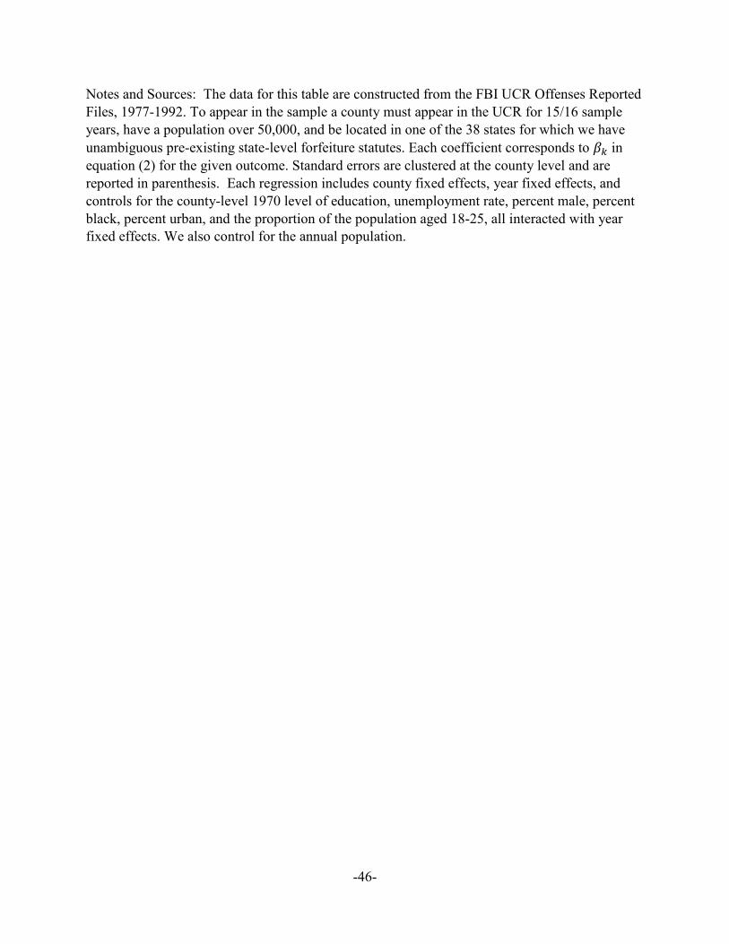
-46-

Notes and Sources: The data for this table are constructed from the FBI UCR Offenses Reported Files, 1977-1992. To appear in the sample a county must appear in the UCR for 15/16 sample years, have a population over 50,000, and be located in one of the 38 states for which we have unambiguous pre-existing state-level forfeiture statutes. Each coefficient corresponds to 𝛽𝑘 in equation (2) for the given outcome. Standard errors are clustered at the county level and are reported in parenthesis. Each regression includes county fixed effects, year fixed effects, and controls for the county-level 1970 level of education, unemployment rate, percent male, percent black, percent urban, and the proportion of the population aged 18-25, all interacted with year fixed effects. We also control for the annual population.

-47-

Table 5: Arrests: Dynamic Effects

Arrests - Dynamic Effects (1) (2) (3) (4)

VARIABLES Total Violent Non-

Violent Drug

(1-pre84keep)*(t=1980) 1,174 43.91 433.5 696.7 (1,733) (635.4) (749.1) (607.8)

(1-pre84keep)*(t=1981) 578.6 188.3 62.60 327.8 (744.8) (399.4) (248.3) (318.3)

(1-pre84keep)*(t=1982) -375.5 -254.9 -310.3 189.7 (559.7) (302.0) (246.7) (190.6)

(1-pre84keep)*(t=1983) 0 0 0 0

(1-pre84keep)*(t=1984) 133.6 -30.42 249.3 -85.26(415.1) (127.6) (197.8) (254.2)

(1-pre84keep)*(t=1985) -16.53 -108.9 48.63 43.77(662.1) (223.3) (373.9) (425.7)

(1-pre84keep)*(t=1986) -671.0 -231.9 -241.6 -197.5(959.3) (331.0) (405.3) (548.6)

(1-pre84keep)*(t=1987) 933.2 -38.85 547.4 424.7(1,707) (533.7) (986.0) (266.3)

(1-pre84keep)*(t=1988) 1,159 64.76 712.9 381.4**(1,496) (493.6) (952.4) (192.9)

(1-pre84keep)*(t=1989) 1,669 105.0 944.2 620.2***(1,580) (506.9) (1,008) (230.8)

(1-pre84keep)*(t=1990) 1,507 -359.2 1,070 795.9***(2,087) (853.3) (1,150) (290.6)

(1-pre84keep)*(t=1991) 1,992 17.78 1,065 909.8**(1,885) (511.9) (1,156) (361.1)

(1-pre84keep)*(t=1992) 1,875 -238.5 1,156 957.2**(1,934) (529.6) (1,185) (372.3)

Observations 2,431 2,431 2,431 2,431 R-squared 0.956 0.949 0.936 0.928 Mean 8170 2418 3801 1951 Clusters 187 187 187 187 Standard errors in parentheses *** p<0.01, ** p<0.05, * p<0.1

Notes and Sources: The data for this table are constructed from the FBI UCR Arrests Files, 1980-1992. To appear in the sample a police jurisdiction must appear in the UCR for 12/13 sample years, have a population over 50,000, and be located in one of the 38 states for which we have unambiguous pre-existing state-level forfeiture statutes. Each coefficient corresponds to 𝛽𝑘 in equation (2) for the given outcome. Standard errors are clustered at the police jurisdiction level and are reported in parenthesis. Each regression includes police jurisdiction fixed effects,

-48-

year fixed effects, and controls for the county-level 1970 level of education, unemployment rate, percent male, percent black, percent urban, and the proportion of the population aged 18-25, all interacted with year fixed effects. We also control for the annual population.

-49-

Table 6: Police Spending and Sworn Officers

Police Expenditures and Sworn Officers – Dynamic Effects (1) (2)

VARIABLES

Police Expenditures ($100,000) Sworn Officers

(1-pre84keep)*(t=1977) -39.07 49.06 (25.60) (48.13)

(1-pre84keep)*(t=1978) -38.05* 26.04 (20.16) (47.69)

(1-pre84keep)*(t=1979) -31.62* 42.76 (16.64) (44.37)

(1-pre84keep)*(t=1980) -25.06* 12.81 (13.26) (52.51)

(1-pre84keep)*(t=1981) -11.42 20.05 (8.074) (51.49)

(1-pre84keep)*(t=1982) -2.150 1.556 (4.065) (51.81)

(1-pre84keep)*(t=1983) 0 0

(1-pre84keep)*(t=1984) 9.530** 3.793 (4.346) (15.47)

(1-pre84keep)*(t=1985) 16.63* -32.75*(9.324) (18.94)

(1-pre84keep)*(t=1986) 20.09 -48.16**(12.30) (22.90)

(1-pre84keep)*(t=1987) 21.90 -57.94**(17.98) (26.46)

(1-pre84keep)*(t=1988) 13.01 -79.21***(18.16) (23.69)

(1-pre84keep)*(t=1989) 20.78 -74.16**(21.22) (29.44)

(1-pre84keep)*(t=1990) 22.43 -75.31**(26.71) (29.82)

(1-pre84keep)*(t=1991) 29.25 -87.23***(32.63) (30.14)

(1-pre84keep)*(t=1992) 46.53 -97.12***(38.18) (33.17)

Observations 9,040 9,376 R-squared 0.936 0.982 Mean 196.2 698.5 Clusters 565 586 Standard errors in parentheses *** p<0.01, ** p<0.05, * p<0.1

-50-

Notes and Sources: Sworn Officer data is drawn from the FBI UCR LEOKA 1977-1992, while Police Expenditure data is from the Census of Government Finances, 1977-1992. To appear in the sample a county must appear in the UCR for 15/16 sample years, have a population over 50,000, and be located in one of the 38 states for which we have unambiguous pre-existing state-level forfeiture statutes. Each coefficient corresponds to 𝛽𝑘 in equation (2) for the given outcome. Standard errors are clustered at the county level and are reported in parenthesis. Each regression includes county fixed effects, year fixed effects, and controls for the county-level 1970 level of education, unemployment rate, percent male, percent black, percent urban, and the proportion of the population aged 18-25, all interacted with year fixed effects. We also control for the annual population

-51-

Table 7: Pre-Trends

Panel A: Offenses Reported - Pre-Trends (1) (2) (3) (4) (5) (6) (7) (8) (9) (10)

VARIABLES Total ViolentNon-

Violent Burglary Larceny Vehicular Murder Rape Robbery Aslt

(Treat*TimeTrend) 93.25 14.01 79.24 6.176 78.37 -5.305 -0.348 -0.113 17.77 -3.646(194.8) (36.08) (160.5) (48.85) (85.62) (41.16) (0.605) (1.524) (22.77) (13.47)

Observations 4,137 4,137 4,137 4,137 4,137 4,137 4,137 4,137 4,137 4,137 R-squared 0.536 0.389 0.555 0.518 0.598 0.393 0.385 0.441 0.350 0.403 Mean 14607 1430 13177 4000 7891 1285 23.82 92.05 615 723.3 Clusters 591 591 591 591 591 591 591 591 591 591 Standard errors in parentheses *** p<0.01, ** p<0.05, * p<0.1

Panel B: Arrests- Pre-Trends (1) (2) (3) (4) (5) (6) (7) (8) (9) (10)

VARIABLES Total ViolentNon-

Violent Drug Robbery Agg

Assault Oth

Assault Burglary Larceny Vehicular

(Treat*TimeTrend) -124.4 -167.0 -104.3 147.0 -21.42 51.25 -192.9 -28.39 -59.29 -16.65(649.3) (240.8) (272.0) (239.7) (24.68) (39.30) (211.5) (66.85) (224.5) (20.32)

Observations 748 748 748 748 748 748 722 748 748 748 R-squared 0.708 0.691 0.694 0.703 0.726 0.708 0.412 0.696 0.641 0.667 Mean 8170 2418 3801 1951 488.7 686.2 1275 865.5 2561 375.4 Clusters 187 187 187 187 187 187 187 187 187 187 Standard errors in parentheses *** p<0.01, ** p<0.05, * p<0.1

Notes and Sources: The data for Panel A are constructed from the FBI UCR Offenses Reported Files, 1977-1983. The data for Panel B are constructed from the FBI UCR Arrests Files, 1980-1983. To appear in the sample a police jurisdiction must appear in the UCR

-52-

for 12/13 sample years, have a population over 50,000, and be located in one of the 38 states for which we have unambiguous pre-existing state-level forfeiture statutes. Each coefficient is from a different regression and reports the relationship corresponding to 𝛽3in equation (3). Standard errors are clustered at the police jurisdiction level and are reported in parenthesis. Each regression includes either county of police jurisdiction fixed effects, year fixed effects, and controls for the county-level 1970 level of education, unemployment rate, percent male, percent black, percent urban, and the proportion of the population aged 18-25, all interacted with year fixed effects. We also control for the annual population.

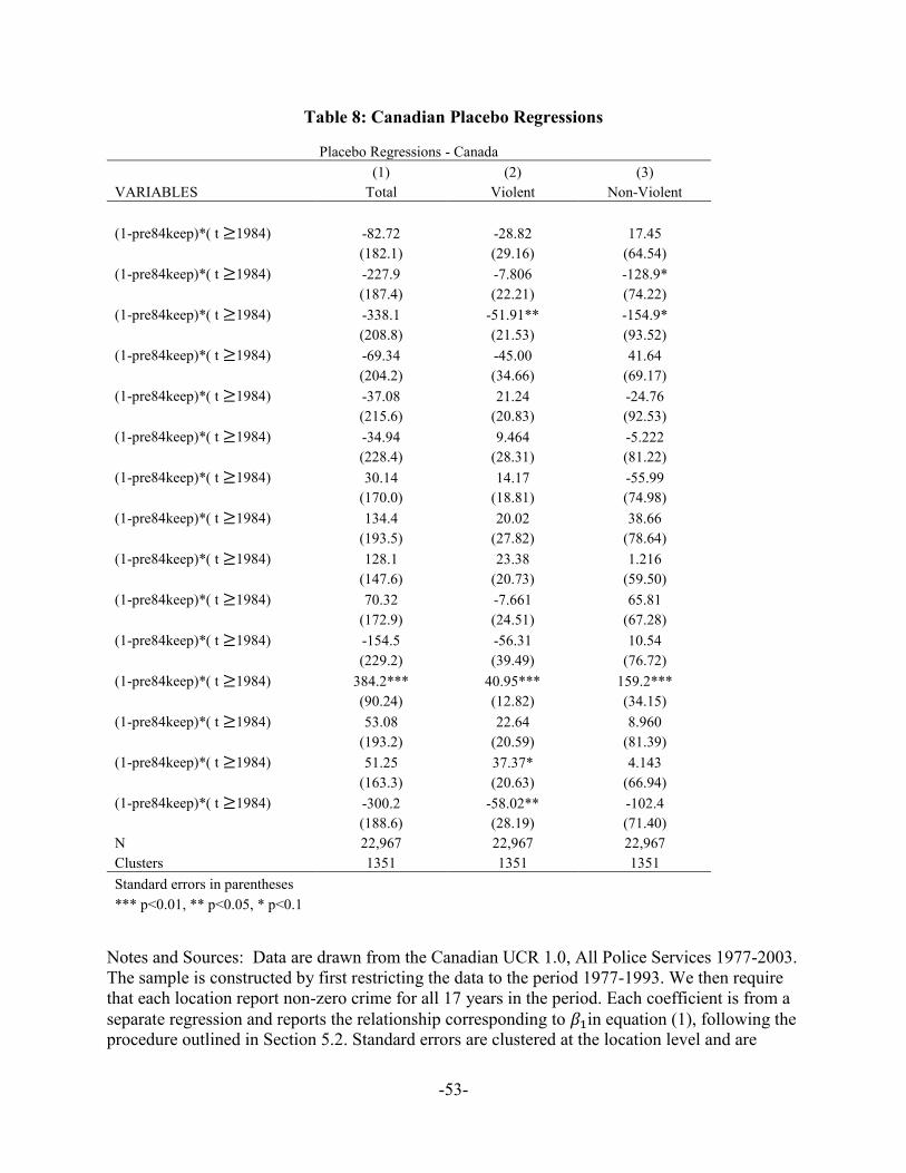
-53-

Table 8: Canadian Placebo Regressions

Placebo Regressions - Canada (1) (2) (3)

VARIABLES Total Violent Non-Violent

(1-pre84keep)*( t ≥1984) -82.72 -28.82 17.45 (182.1) (29.16) (64.54)

(1-pre84keep)*( t ≥1984) -227.9 -7.806 -128.9*(187.4) (22.21) (74.22)

(1-pre84keep)*( t ≥1984) -338.1 -51.91** -154.9*(208.8) (21.53) (93.52)

(1-pre84keep)*( t ≥1984) -69.34 -45.00 41.64(204.2) (34.66) (69.17)

(1-pre84keep)*( t ≥1984) -37.08 21.24 -24.76(215.6) (20.83) (92.53)

(1-pre84keep)*( t ≥1984) -34.94 9.464 -5.222(228.4) (28.31) (81.22)

(1-pre84keep)*( t ≥1984) 30.14 14.17 -55.99(170.0) (18.81) (74.98)

(1-pre84keep)*( t ≥1984) 134.4 20.02 38.66(193.5) (27.82) (78.64)

(1-pre84keep)*( t ≥1984) 128.1 23.38 1.216(147.6) (20.73) (59.50)

(1-pre84keep)*( t ≥1984) 70.32 -7.661 65.81(172.9) (24.51) (67.28)

(1-pre84keep)*( t ≥1984) -154.5 -56.31 10.54(229.2) (39.49) (76.72)

(1-pre84keep)*( t ≥1984) 384.2*** 40.95*** 159.2***(90.24) (12.82) (34.15)

(1-pre84keep)*( t ≥1984) 53.08 22.64 8.960 (193.2) (20.59) (81.39)

(1-pre84keep)*( t ≥1984) 51.25 37.37* 4.143 (163.3) (20.63) (66.94)

(1-pre84keep)*( t ≥1984) -300.2 -58.02** -102.4(188.6) (28.19) (71.40)

N 22,967 22,967 22,967Clusters 1351 1351 1351Standard errors in parentheses *** p<0.01, ** p<0.05, * p<0.1

Notes and Sources: Data are drawn from the Canadian UCR 1.0, All Police Services 1977-2003. The sample is constructed by first restricting the data to the period 1977-1993. We then require that each location report non-zero crime for all 17 years in the period. Each coefficient is from a separate regression and reports the relationship corresponding to 𝛽1in equation (1), following the procedure outlined in Section 5.2. Standard errors are clustered at the location level and are

-54-

reported in parenthesis. Specifically, we randomly assign pre-1984 forfeiture retention rates to Canadian provinces based on the pre-1984 distribution in the United States. We report the coefficients from 15 different permutations of this exercise.

-55-

Table 9: Offenses Reported – Additional Controls

Offenses Reported - Additional Controls OUTCOME (1) (2) (3) (4)Total Crime -2,691*** -2,820*** -2,386*** -2,760***

(757.4) (783.7) (726.9) (740.1)Violent 87.06 49.36 -252.2* 50.94

(188.2) (176.0) (140.4) (175.2) Non-Violent -2,779*** -2,869*** -2,134*** -2,811***

(727.9) (735.4) (676.2) (722.3)Burglary -1,053*** -1,121*** -469.8* -1,058***

(315.8) (320.9) (260.1) (317.1)Larceny -1,631*** -1,648*** -1,324*** -1,646***

(411.5) (407.0) (396.6) (409.5)Federal Defendant Control N Y N N State Incarceration Controls N N Y N 1960s Race Riot Controls N N N Y Observations 9,449 9,449 9,449 9,449 Clusters 591 591 591 591 Standard errors in parenthesis *** p<0.01, ** p<0.05, * p<0.1

Notes and Sources: See notes to Table 1. Column (1) reports the main results from Table 1, Panel A. Column (2) controls for the number of inmates at the state level, measured in 1981. Column (3) controls for the share of federal defendants originating in the state. Both the inmate and federal defendant data are drawn from the DOJ’s Sourcebook of Criminal Justice Statistics (1981). Column (4) controls for the number of race riots that took place in the county during the 1960’s drawing on data reported in Carter (1986) and Collins and Margo (2007). The three sets of additional control variables are interacted with the full set of year fixed effects.

-56-

Table 10: Offenses Reported – Heterogeneous Effects

Heterogeneous Effects by Population and Percent Black Population Percent Black

(1) (2) (3) (4) (5) (1) (2) (3) (4) (5)

VARIABLES Total ViolentNon-

Violent Burglary Larceny Total Violent Non-

Violent Burglary Larceny

(1-pre84keep)*(year>1984) -2,288* -948.8** -1,339 250.5 -1,103** -2,297*** -92.56 -2,204*** -596.5** -1,444***(1,366) (391.4) (994.9) (474.6) (457.8) (690.1) (142.3) (660.7) (263.0) (412.3)

(1-pre84keep)* Post84* Population -0.00101 0.00342** -0.00443 -0.00419** -0.00158(0.00510) (0.00138) (0.00373) (0.00176) (0.00163)

(1-pre84keep)* Post84*Percent Black -2,738 1,745 -4,483 -3,958* -1,281(5,288) (1,774) (4,733) (2,303) (2,866)

Observations 9,449 9,449 9,449 9,449 9,449 9,449 9,449 9,449 9,449 9,449 R-squared 0.984 0.960 0.985 0.977 0.983 0.984 0.951 0.984 0.970 0.983 Mean 15493 1710 13783 3804 8429 15493 1710 13783 3804 8429 Clusters 591 591 591 591 591 591 591 591 591 591 Robust standard errors in parentheses *** p<0.01, ** p<0.05, * p<0.1

Notes and Sources: See notes to Table 1.

-57-

Table 11: Housing Values

Census County Level Data FHFA State Level (1) (2) (3) (4)

VARIABLES Median House

Value Log(Median House

Value) HPI Log(HPI)

(1-Pre84Keep) *(year>1984) 9,289*** 0.0167** 13.72 0.0899* (817.9) (0.00794) (9.110) (0.0521)

Observations 7,995 7,993 2,583 2,583 R-squared 0.877 0.981 0.902 0.930 Mean 33547 10.15 128.6 4.807 Clusters 2666 2665 38 38 Standard errors in parentheses *** p<0.01, ** p<0.05, * p<0.1

Notes and Sources: Each coefficient corresponds to 𝛽1 in equation (1) for the given housing value outcome. The results reported in Columns (1) and (2) use county-level data drawn from the Census of Population in 1970, 1980, and 1990. Standard errors are reported in parenthesis and are clustered at the county level. Columns (3) and (4) utilize quarterly, state-level price indices, from 1977 to 1993 from the Federal Housing Financial Agency (https://www.fhfa.gov/DataTools/Downloads/Pages/House-Price-Index-Datasets.aspx#mpo). Standard errors are reported in parenthesis and are clustered at the state level. As in other specifications, we restrict the sample to the 38 states that report unambiguous forfeiture statutes. Each regression includes location fixed effects and year fixed effects.

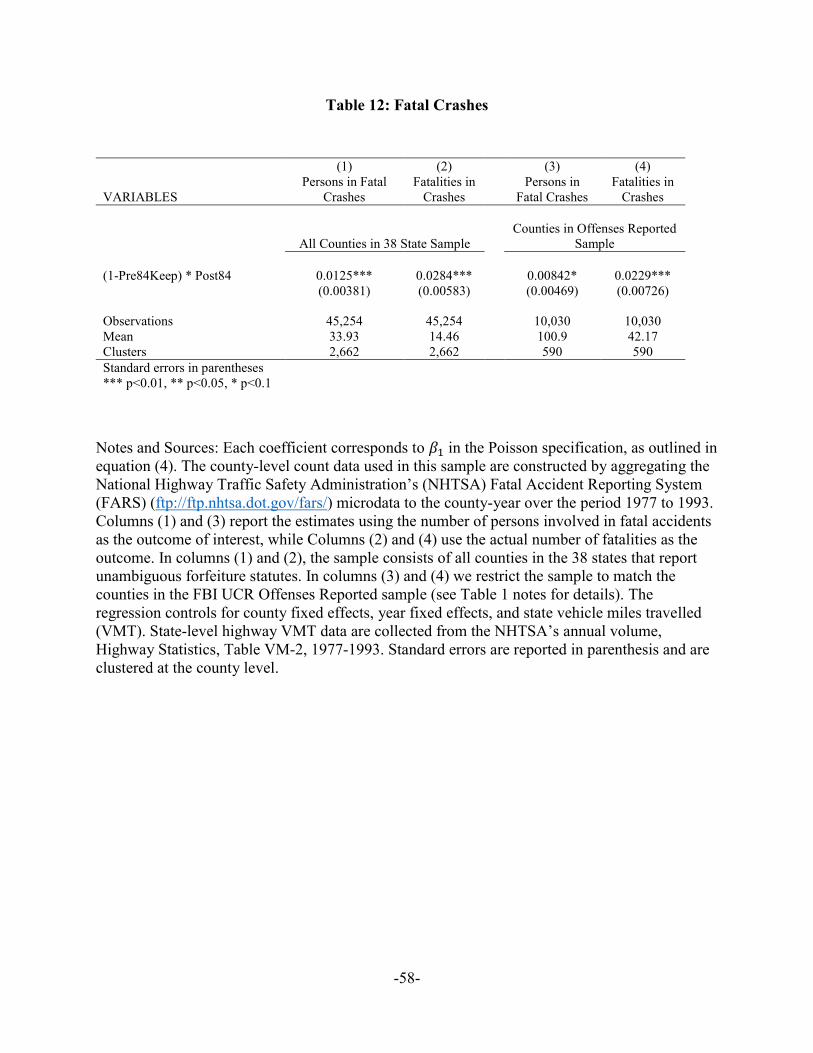
-58-

Table 12: Fatal Crashes

(1) (2) (3) (4)

VARIABLES Persons in Fatal

Crashes Fatalities in

Crashes Persons in

Fatal Crashes Fatalities in

Crashes

All Counties in 38 State Sample Counties in Offenses Reported

Sample

(1-Pre84Keep) * Post84 0.0125*** 0.0284*** 0.00842* 0.0229*** (0.00381) (0.00583) (0.00469) (0.00726)

Observations 45,254 45,254 10,030 10,030 Mean 33.93 14.46 100.9 42.17 Clusters 2,662 2,662 590 590 Standard errors in parentheses *** p<0.01, ** p<0.05, * p<0.1

Notes and Sources: Each coefficient corresponds to 𝛽1 in the Poisson specification, as outlined in equation (4). The county-level count data used in this sample are constructed by aggregating the National Highway Traffic Safety Administration’s (NHTSA) Fatal Accident Reporting System (FARS) (ftp://ftp.nhtsa.dot.gov/fars/) microdata to the county-year over the period 1977 to 1993. Columns (1) and (3) report the estimates using the number of persons involved in fatal accidents as the outcome of interest, while Columns (2) and (4) use the actual number of fatalities as the outcome. In columns (1) and (2), the sample consists of all counties in the 38 states that report unambiguous forfeiture statutes. In columns (3) and (4) we restrict the sample to match the counties in the FBI UCR Offenses Reported sample (see Table 1 notes for details). The regression controls for county fixed effects, year fixed effects, and state vehicle miles travelled (VMT). State-level highway VMT data are collected from the NHTSA’s annual volume, Highway Statistics, Table VM-2, 1977-1993. Standard errors are reported in parenthesis and are clustered at the county level.

-59-

Appendix Tables

Table A1: State Level Civil Forfeiture Sources

Pre-CCCA State Civil Forfeiture Statutes Sources State Link Alabama http://heinonline.org/HOL/Page?men_tab=srchresults&handle=hein.ssl/ssal0075&size=2&collection=ssl&id=205 Alaska http://heinonline.org/HOL/Page?men_tab=srchresults&handle=hein.ssl/ssak0051&size=2&collection=ssl&id=433 Arizona http://heinonline.org/HOL/Page?men_tab=srchresults&handle=hein.ssl/ssaz0050&size=2&collection=ssl&id=444 Arkansas http://heinonline.org/HOL/Page?men_tab=srchresults&handle=hein.ssl/ssar0089&size=2&collection=ssl&id=956 California http://heinonline.org/HOL/Page?men_tab=srchresults&handle=hein.ssl/ssca0108&size=2&collection=ssl&id=461 Colorado http://heinonline.org/HOL/Page?men_tab=srchresults&handle=hein.ssl/ssco0098&size=2&collection=ssl&id=534 Connecticut http://heinonline.org/HOL/Page?men_tab=srchresults&handle=hein.ssl/ssct0123&size=2&collection=ssl&id=332 Delaware http://heinonline.org/HOL/Page?men_tab=srchresults&handle=hein.ssl/ssde0025&size=2&collection=ssl&id=621 Florida http://heinonline.org/HOL/Page?men_tab=srchresults&handle=hein.ssl/ssfl0117&size=2&collection=ssl&id=35 Georgia http://heinonline.org/HOL/Page?men_tab=srchresults&handle=hein.ssl/ssga0090&size=2&collection=ssl&id=502 Hawaii http://heinonline.org/HOL/Page?men_tab=srchresults&handle=hein.ssl/sshi0027&size=2&collection=ssl&id=377 Idaho http://heinonline.org/HOL/Page?men_tab=srchresults&handle=hein.ssl/ssid0052&size=2&collection=ssl&id=693 Illinois http://heinonline.org/HOL/Page?men_tab=srchresults&handle=hein.ssl/ssil0107&size=2&collection=ssl&id=1306 Indiana http://heinonline.org/HOL/Page?men_tab=srchresults&handle=hein.ssl/ssin0119&size=2&collection=ssl&id=631 Iowa http://heinonline.org/HOL/Page?men_tab=srchresults&handle=hein.ssl/ssia0029&size=2&collection=ssl&id=273 Kansas http://heinonline.org/HOL/Page?men_tab=srchresults&handle=hein.ssl/ssks0042&size=2&collection=ssl&id=1189 Kentucky http://heinonline.org/HOL/Page?men_tab=srchresults&handle=hein.ssl/ssky0115&size=2&collection=ssl&id=160 Louisiana http://heinonline.org/HOL/Page?men_tab=srchresults&handle=hein.ssl/ssla0103&size=2&collection=ssl&id=104 Maine http://heinonline.org/HOL/Page?men_tab=srchresults&handle=hein.ssl/ssme0068&size=2&collection=ssl&id=946 Maryland http://heinonline.org/HOL/Page?men_tab=srchresults&handle=hein.ssl/ssmd0197&size=2&collection=ssl&id=2460 Massachusetts http://heinonline.org/HOL/Page?handle=hein.ssl/ssma0060&start_page=1&collection=ssl&id=705 Michigan http://heinonline.org/HOL/Page?men_tab=srchresults&handle=hein.ssl/ssmi0039&size=2&collection=ssl&id=778 Minnesota http://heinonline.org/HOL/Page?men_tab=srchresults&handle=hein.ssl/ssmn0072&size=2&collection=ssl&id=359 Mississippi http://heinonline.org/HOL/Page?men_tab=srchresults&handle=hein.ssl/ssms0108&size=2&collection=ssl&id=920

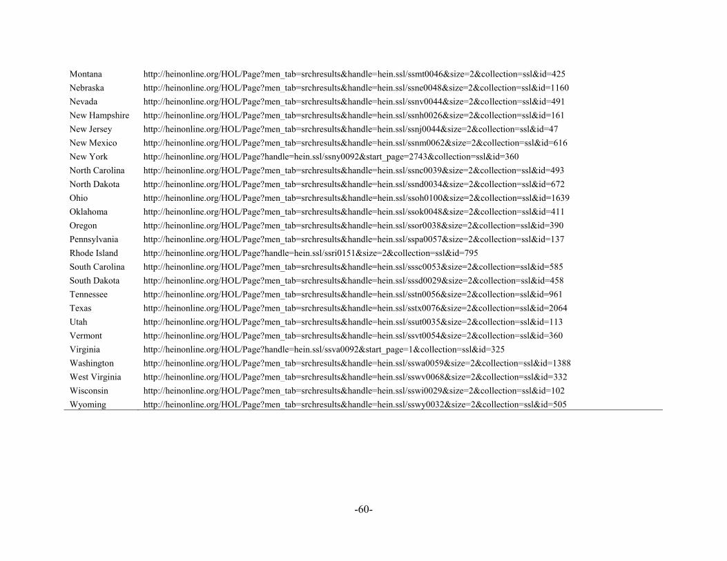
-60-

Montana http://heinonline.org/HOL/Page?men_tab=srchresults&handle=hein.ssl/ssmt0046&size=2&collection=ssl&id=425 Nebraska http://heinonline.org/HOL/Page?men_tab=srchresults&handle=hein.ssl/ssne0048&size=2&collection=ssl&id=1160 Nevada http://heinonline.org/HOL/Page?men_tab=srchresults&handle=hein.ssl/ssnv0044&size=2&collection=ssl&id=491 New Hampshire http://heinonline.org/HOL/Page?men_tab=srchresults&handle=hein.ssl/ssnh0026&size=2&collection=ssl&id=161 New Jersey http://heinonline.org/HOL/Page?men_tab=srchresults&handle=hein.ssl/ssnj0044&size=2&collection=ssl&id=47 New Mexico http://heinonline.org/HOL/Page?men_tab=srchresults&handle=hein.ssl/ssnm0062&size=2&collection=ssl&id=616 New York http://heinonline.org/HOL/Page?handle=hein.ssl/ssny0092&start_page=2743&collection=ssl&id=360 North Carolina http://heinonline.org/HOL/Page?men_tab=srchresults&handle=hein.ssl/ssnc0039&size=2&collection=ssl&id=493 North Dakota http://heinonline.org/HOL/Page?men_tab=srchresults&handle=hein.ssl/ssnd0034&size=2&collection=ssl&id=672 Ohio http://heinonline.org/HOL/Page?men_tab=srchresults&handle=hein.ssl/ssoh0100&size=2&collection=ssl&id=1639 Oklahoma http://heinonline.org/HOL/Page?men_tab=srchresults&handle=hein.ssl/ssok0048&size=2&collection=ssl&id=411 Oregon http://heinonline.org/HOL/Page?men_tab=srchresults&handle=hein.ssl/ssor0038&size=2&collection=ssl&id=390 Pennsylvania http://heinonline.org/HOL/Page?men_tab=srchresults&handle=hein.ssl/sspa0057&size=2&collection=ssl&id=137 Rhode Island http://heinonline.org/HOL/Page?handle=hein.ssl/ssri0151&size=2&collection=ssl&id=795 South Carolina http://heinonline.org/HOL/Page?men_tab=srchresults&handle=hein.ssl/sssc0053&size=2&collection=ssl&id=585 South Dakota http://heinonline.org/HOL/Page?men_tab=srchresults&handle=hein.ssl/sssd0029&size=2&collection=ssl&id=458 Tennessee http://heinonline.org/HOL/Page?men_tab=srchresults&handle=hein.ssl/sstn0056&size=2&collection=ssl&id=961 Texas http://heinonline.org/HOL/Page?men_tab=srchresults&handle=hein.ssl/sstx0076&size=2&collection=ssl&id=2064 Utah http://heinonline.org/HOL/Page?men_tab=srchresults&handle=hein.ssl/ssut0035&size=2&collection=ssl&id=113 Vermont http://heinonline.org/HOL/Page?men_tab=srchresults&handle=hein.ssl/ssvt0054&size=2&collection=ssl&id=360 Virginia http://heinonline.org/HOL/Page?handle=hein.ssl/ssva0092&start_page=1&collection=ssl&id=325 Washington http://heinonline.org/HOL/Page?men_tab=srchresults&handle=hein.ssl/sswa0059&size=2&collection=ssl&id=1388 West Virginia http://heinonline.org/HOL/Page?men_tab=srchresults&handle=hein.ssl/sswv0068&size=2&collection=ssl&id=332 Wisconsin http://heinonline.org/HOL/Page?men_tab=srchresults&handle=hein.ssl/sswi0029&size=2&collection=ssl&id=102 Wyoming http://heinonline.org/HOL/Page?men_tab=srchresults&handle=hein.ssl/sswy0032&size=2&collection=ssl&id=505

-61-

Table A2: Summary Statistics of 𝑿𝒊,𝟏𝟗𝟕𝟎 Characteristics

Summary Statistics of 1970 Census Characteristics (1) (2) (3) (3)-(2)

Variable Whole Sample Control County

Treated County Difference

Population Share Aged 18-25 47.50 47.49 47.52 -0.0308Education - Less than High School 23.19 22.94 24.45 -1.5054Education - High School Graduate 15.68 15.99 14.09 1.9065Education - Some College 5.10 5.03 5.41 -0.3728Education - College Graduate 5.09 5.10 5.09 0.0053Unemployment Rate 1.58 1.62 1.42 0.1996Poverty Rate 0.68 0.63 0.94 -0.3105Percent Male 49.05 49.04 49.11 -0.0694Percent Black 8.69 7.78 13.32 -5.5350Percent Urban 36.96 36.56 38.99 -2.4271Bold Indicates Statistically Significant Difference at the 5 percent level.

Notes and Sources: This table reports the mean for each of the 1970 Census of Population variables that are used as covariates in Equation (1). Column (1) reports the mean for all 591 counties in the sample, while Columns (2) and (3) report the means in Control and Treatment counties respectively. Column (4) reports the difference in means between the treatment and control counties, differences shown in bold typeface indicate a statistically significant difference at the 5 percent level.

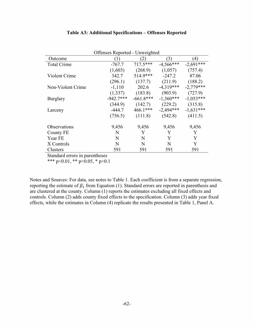
-62-

Table A3: Additional Specifications – Offenses Reported

Offenses Reported - Unweighted Outcome (1) (2) (3) (4)Total Crime -767.7 717.5*** -4,566*** -2,691***

(1,603) (268.9) (1,057) (757.4) Violent Crime 342.7 514.9*** -247.2 87.06

(296.1) (137.7) (211.9) (188.2) Non-Violent Crime -1,110 202.6 -4,319*** -2,779***

(1,337) (183.8) (903.9) (727.9)Burglary -942.7*** -661.8*** -1,360*** -1,053***

(344.9) (142.7) (229.2) (315.8) Larceny -444.7 466.1*** -2,494*** -1,631***

(756.5) (111.8) (542.8) (411.5)

Observations 9,456 9,456 9,456 9,456 County FE N Y Y Y Year FE N N Y Y X Controls N N N Y Clusters 591 591 591 591 Standard errors in parentheses *** p<0.01, ** p<0.05, * p<0.1

Notes and Sources: For data, see notes to Table 1. Each coefficient is from a separate regression, reporting the estimate of 𝛽1 from Equation (1). Standard errors are reported in parenthesis and are clustered at the county. Column (1) reports the estimates excluding all fixed effects and controls. Column (2) adds county fixed effects to the specification. Column (3) adds year fixed effects, while the estimates in Column (4) replicate the results presented in Table 1, Panel A.

-63-

Table A4: Additional Specifications – Arrests

Arrests - Unweighted OUTCOME (1) (2) (3) (4)Total Arrests 811.7 -1,346*** -426.8 598.2

(1,238) (244.0) (395.5) (705.8) Violent Arrests 550.2 -227.9*** -416.9*** -86.38

(407.4) (86.86) (136.0) (188.6)Non-Violent Arrests -636.6* -1,496*** -520.1 564.6

(378.3) (351.6) (467.8) (655.7)Drug 898.0* 378.2* 510.2** 120.0

(542.2) (219.4) (243.0) (296.5)Robbery 32.96 -220.9*** -161.6* 82.27

(97.67) (82.49) (91.72) (121.5)Agg. Assault 208.2 26.64 78.22 140.2**

(141.3) (42.08) (50.59) (70.33)Other Assault 302.2 3.375 -224.0** -255.4**

(226.9) (60.38) (94.71) (112.2)Burglary -259.1*** -586.7*** -225.1 241.1

(78.42) (157.2) (188.6) (230.8)Larceny -464.8* -880.1*** -294.3 213.3

(262.2) (180.4) (260.3) (376.3)Vehicular 87.29 -29.56 -0.717 110.2

(69.13) (35.44) (51.36) (77.04)

Observations 2,431 2,431 2,431 2,431 County FE N Y Y Y Year FE N N Y Y X Controls N N N Y Clusters 187 187 187 187 Robust standard errors in parentheses *** p<0.01, ** p<0.05, * p<0.1

Notes and Sources: For data, see notes to Table 2. Each coefficient is from a separate regression, reporting the estimate of 𝛽1 from Equation (1). Standard errors are reported in parenthesis and are clustered at the county. Column (1) reports the estimates excluding all fixed effects and controls. Column (2) adds county fixed effects to the specification. Column (3) adds year fixed effects, while the estimates in Column (4) replicate the results presented in Table 2, Panel A.

-64-

Table A5: Offenses Reported-Assign Ambiguous States

Offenses Reported - Assign Ambiguous States Outcome (1) (2) (3) Total Crime -2,691*** -2,709*** -1,225***

(757.4) (715.3) (444.3)Violent Crime 87.06 1.369 246.8

(188.2) (166.6) (153.5) Non-Violent Crime -2,779*** -2,710*** -1,472***

(727.9) (691.2) (421.4)Burglary -1,053*** -1,039*** -655.2***

(315.8) (290.8) (211.9)Larceny -1,631*** -1,544*** -834.8***

(411.5) (397.2) (246.2)Observations 9,456 11,664 11,664Ambig. State Rate N/A 0 100 Clusters 591 729 729 Standard errors in parentheses *** p<0.01, ** p<0.05, * p<0.1

Notes and Sources: For data, see notes to Table 1. Each coefficient is from a separate regression, reporting the estimate of 𝛽1 from Equation (1). Standard errors are reported in parenthesis and are clustered at the county. Column (1) replicates the main results from Table 1, Panel A. Column (2) assumes that the retention rate for seized assets is 0 percent in the states with missing forfeiture data. Column (3) assumes that the retention rate for seized assets is 100 percent in the states with missing forfeiture data.

-65-

Table A6: Arrests – Assign Ambiguous States

Arrests - Assign Ambiguous States Outcome (1) (2) (3) Total 598.2 223.3 -753.5**

(705.8) (601.0) (346.0)Violent -86.38 -38.04 -298.9***

(188.6) (117.6) (106.4)Non-Violent 564.6 181.9 -599.9*

(655.7) (519.3) (324.0)Drug 120.0 79.51 145.2

(296.5) (112.3) (172.0)Robbery 82.27 -13.09 -142.1**

(121.5) (82.72) (65.48)Agg. Assault 140.2** 43.51 -16.72

(70.33) (40.68) (36.33)Assault -255.4** -76.78 -133.2

(112.2) (51.18) (85.05)Burglary 241.1 53.99 -237.2**

(230.8) (169.2) (119.1)Larceny 213.3 47.71 -353.3**

(376.3) (295.5) (178.0)Vehicular 110.2 80.17 -9.317

(77.04) (65.25) (39.62)Observations 2,431 2,990 2,990Ambig. State Rate N/A 0 100 Clusters 187 230 230 Standard errors in parentheses *** p<0.01, ** p<0.05, * p<0.1

Notes and Sources: For data, see notes to Table 2. Each coefficient is from a separate regression, reporting the estimate of 𝛽1 from Equation (1). Standard errors are reported in parenthesis and are clustered at the county. Column (1) replicates the main results from Table 2, Panel A. Column (2) assumes that the retention rate for seized assets is 0 percent in the states with missing forfeiture data. Column (3) assumes that the retention rate for seized assets is 100 percent in the states with missing forfeiture data.