Class 1: Getting started with R

You must read this document while sitting at the computer with Rstudioopen. You will learn by typing in code from these chapters. You can learnfurther by playing with the code.

Computing is central to modern statistics at all levels, from basic to advanced.If you already know how to program, great. If not, consider this a start.

We do our computing in the open-source package R, a command-based statisticalsoftware environment that you can download and operate on your own computer,using Rstudio, a free graphical user interface for R.

Downloading and setting up R and Rstudio

Go to the home of R, http://www.r-project.org/ and click on the “download R”link. This will take you to a list of mirror sites. Choose any of these. Now click onthe link under “Download and Install R” at the top of the page for your operatingsystem (Linux, Mac, or Windows) and download the binaries corresponding to yoursystem. Follow all the instructions. Default settings should be fine.

Go to the home of Rstudio, http://www.rstudio.com, click on “Download RStu-dio,” click on “Download RStudio Desktop,” and click on the installer for yourplatform (Windows, Mac, etc.) Then a download will occur.

When the download is done, click on the RStudio icon to start an R session.To check that R is working, go to the Console window within RStudio. There

should be a “>” prompt. Type 2+5 and hit Enter. You should get [1] 7. From nowon, when we say “type” , we mean type (or copy-and-paste) into the Rconsole and hit Enter.

You will also want to install some R packages, in particular, foreign (whichallows you to read in files formatted for various other statistics packages, includingStata), knitr (which allows you to process certain R documentation), and arm

(which has convenient functions for fitting and displaying some regression models).You can do this from Rstudio by clicking on the Tools tab and then on Installpackages and then entering the names of the packages and clicking Install. Whenyou want to use a package, you load it during your R session as needed, for exampleby typing library("foreign") or library("arm").

Try a few things, typing these one line at a time and looking at the results onthe console:

1/3

sqrt(2)

curve(x^2 + 5, from=-2, to=2)

These will return, respectively, 0.3333333, 1.414214, and a new graphics windowplotting the curve y = x2 + 5.

Finally, quit your R session by closing the Rstudio window.

Calling functions and getting help

Open R and play around, using the assignment function (“<-”). To start, type thefollowing lines into your script.R file and copy-and-paste them into the R window:

1

GETTING STARTED WITH R 2

a <- 3

print(a)

b <- 10

print(b)

a + b

a*b

exp(a)

10^a

log(b)

log10(b)

a^b

round(3.435, 0)

round(3.435, 1)

round(3.435, 2)

R is based on functions, which include mathematical operations (exp(), log(),sqrt(), and so forth) and lots of other routines (print(), round(), . . . ).

The function c() combines things together into a vector. For example, typec(4,10,-1,2.4) in the R console or copy-and-paste the following:

x <- c(4,10,-1,2.4)

print(x)

The function seq() creates an equally-spaced sequence of numbers; for example,seq(4,54,10) returns the sequence from 4, 14, 24, 34, 44, 54. The seq() functionworks with non-integers as well: try seq(0,1,0.1) or seq(2,-5,-0.4). For inte-gers, a:b is shorthand for seq(a,b,1) if b> a, or seq(b,a,-1) if b< a. Let’s trya few more commands:

c(1, 3, 5)

1:5

c(1:5, 1, 3, 5)

c(1:5, 10:20)

seq(2, 10, 2)

seq(1,9,2)

You can get help on any function using “?” in R. For example, type ?seq. Thisshould open an internet browser window with a help file for seq(). R help filestypically have more information than you’ll know what to do with, but if you scrollto the bottom of the page you’ll find some examples that you can cut and pasteinto your console.

Whenever you are trying out a new function, we recommend using “?” to viewthe help file and running the examples at the bottom to see what happens.

Sampling and random numbers

Here’s how to get a random number, uniformly distributed between 0 and 100:

runif(1, 0, 100)

And now 50 more random numbers:

runif(50, 0, 100)

Suppose we want to pick one of three colors with equal probability:

color <- c("blue", "red", "green")

sample(color, 1)

Suppose we want to sample with unequal probabilities:

GETTING STARTED WITH R 3

color <- c("blue", "red", "green")

p <- c(0.5, 0.3, 0.2)

sample(color, 1, prob=p)

Or we can do it all in one line, which is more compact but less readable:

sample(c("blue","red","green"), 1, prob=c(0.5,0.3,0.2))

Data types

Numeric data. In R, numbers are stored as numeric data. This includes many ofthe examples above as well as special constants such as pi.

Big and small numbers. R recognizes scientific notation. A million can be typedin as 1000000 or 1e6, but not as 1,000,000. (R is particular about certain things.Capitalization matters, “,” doesn’t belong in numbers, and spaces usually aren’timportant.) Scientific notation also works for small numbers: 1e-6 is 0.000001 and4.3e-6 is 0.0000043.

Infinity. Type (or copy-and-paste) these into R, one line at a time, and see whathappens:

1/0

-1/0

exp(1000)

exp(-1000)

1/Inf

Inf + Inf

-Inf - Inf

0/0

Inf - Inf

Those last two operations return NaN (Not a Number); type ?Inf for more on thetopic. In general we try to avoid working with infinity but it is convenient to haveInf for those times when we accidentally divide by 0 or perform some other illegalmathematical operation.

Missing data. In R, NA is a special keyword that represents missing data. For moreinformation, type ?NA. Try these commands in R:

NA

2 + NA

NA - NA

NA / NA

NA * NA

c(NA, NA, NA)

c(1, NA, 3)

10 * c(1, NA, 3)

NA / 0

NA + Inf

is.na(NA)

is.na(c(1, NA, 3))

The is.na() function tests whether or not the argument is NA. The last line operateson each element of the vector and returns a vector with three values that indicatewhether the corresponding input is NA.

Character strings. Let’s sample a random color and a random number and putthem together:

GETTING STARTED WITH R 4

color <- sample(c("blue","red","green"), 1, prob=c(0.5,0.3,0.2))

number <- runif(1, 0, 100)

paste(color, number)

Here’s something prettier:

paste(color, round(number,0))

TRUE, FALSE, and ifelse

Try typing these:

2 + 3 == 4

2 + 3 == 5

1 < 2

2 < 1

In R, the expressions ==, <, > are comparisons and return a logical value, TRUEor FALSE as appropriate. Other comparisons include <= (less than or equal), >=(greater than or equal), and != (not equal).

Comparisons can be used in combination with the ifelse() function. The firstargument takes a logical statement, the second argument is an expression to beevaluated if the statement is true, and the third argument is evaluated if the state-ment is false. Suppose we want to pick a random number between 0 and 100 andthen choose the color red if the number is below 30 or blue otherwise:

number <- runif(1, 0, 100)

color <- ifelse(number<30, "red", "blue")

Loops

A key aspect of computer programming is looping—that is, setting up a series ofcommands to be performed over and over. Start by trying out the simplest possibleloop:

for (i in 1:10){

print("hello")

}

Or:

for (i in 1:10){

print(i)

}

Or:

for (i in 1:10){

print(paste("hello", i))

}

The curly braces define what is repeated in the loop.Here’s a loop of random colors:

for (i in 1:10){

number <- runif(1, 0, 100)

color <- ifelse(number<30, "red", "blue")

print(color)

}

Class 2: Reading, writing, and looking at data in R

Your working directory

Choose a working directory on your computer where you will do your R work.Suppose your working directory is c:/myfiles/stat/. Then you should put allyour data files in this directory, and all the files and graphs you save in R willappear here too. To set your working directory in Rstudio, click on the Sessiontab and then on Set Working Directory and then on Choose Directory and thennavigate from there.

Rstudio has several subwindows: a text editor, the R console, a graphics window,and a help window. It’s generally best to type your commands into the Rstudiotext editor and then copy and paste into the R console. When your session is over,you can save the contents of the text editor into a plain-text file with a name suchas todays work.R that you can save in your working directory.

Now go to the R console and type getwd(). This shows your current R workingdirectory. Change your working directory by typing setwd("c:/myfiles/stat/"),or whatever you would like to use.

Then type getwd() in the R console. This should return your working directory(for example, c:/myfiles/stat/).

Reading data

Let’s read some data into R. The file heads.csv has data from a coin flippingexperiment done in a previous class. Each student flipped a coin 10 times and wehave a count of the number of students who saw exactly 0, 1, 2, . . . , 10 heads. The fileis located at the website http://www.stat.columbia.edu/~gelman/bda.course/.Start by going to this location, downloading the file, and saving it as heads.csv inyour working directory (for example, c:/myfiles/stat/).

Now read the file into R:

heads <- read.csv("heads.csv")

R can also read the file directly from the web rather than saving it to your computerfirst. For example:

heads <- read.csv("http://www.stat.columbia.edu/~gelman/bda.course/heads.csv")

Typing the name of any object in R displays the object itself. So type heads andlook at what comes out.

Now for a longer file: download nycData.csv from http://www.stat.columbia.

edu/~gelman/bda.course/, save it in your working directory, and read it in:

nyc <- read.csv("nycData.csv")

This data is a subset of U.S. census data from New York City zip codes. If you nowtype nyc from the console, the file will scroll off the screen: it’s too big! Instead,let’s just look at the first 5 rows:

nyc[1:5, ]

We’ll talk in a bit about what to do with these data, but first we’ll consider someother issues involving data input.

What if you have tabular data separated by spaces and tabs, rather than columns?For example, mile.txt from http://www.stat.columbia.edu/~gelman/bda.course/.You just use the read.table() function:

5

READING, WRITING, AND LOOKING AT DATA IN R 6

mile <- read.table("mile.txt", header=TRUE)

mile[1:5, ]

The header=TRUE argument is appropriate here because the first line of the filemile.txt is a “header,” that is, a list of column names. If the file had just datawith no header, we would simply call read.table("mile.txt") with no headerargument.

Writing data

You can save data into a file using write instead of read. For example, to writethe R object heads into a comma-separated file output1.csv, we would typewrite.csv(heads,"output1.csv"). To write it into a space-separated file out-put2.txt, it’s just write.table(heads,"output2.txt").

Examining data

At this point, we should have three variables in our R environment, heads, nyc,and miles. We can see what we have in our session by clicking on the Environmenttab in the Rstudio window.

Data frames, vectors, and subscripting. Most of the functions used to read data re-turn a data structure called a data frame. You can see this by typing class(heads).Each column of a data frame is a vector. We can access the first column of headsby typing heads[,1]. Data frames are indexed using two vectors inside “[” and“]”; the two vectors are separated by a comma. The first vector indicates whichrows you are interested in and the second vector indicates what columns you areinterested in. For example, heads[6,1] shows the number of heads observed andheads[6,2] shows the number of students that observed that number of heads.Leaving it blank is shorthand for including all. Try:

heads[6,]

heads[1:3,]

heads[,1]

heads[,1:2]

heads[,]

To find the number of columns in a data frame, use the function length(). To findthe number of rows, use nrow(). We can also find the names of the columns byusing names(). Try these:

length(heads)

nrow(heads)

names(heads)

length(nyc)

nrow(nyc)

names(nyc)

We can also index a column within a data frame by using $. The call to names(nyc)

showed the names of the 7 columns in the data set. We can access the zip codesby typing nyc$zipcode or the population of each of the zip codes by typingnyc$pop.total. As we mentioned before, these columns are vectors. We can in-dex these vectors like any other vectors. Try:

nyc$zipcode[1:5]

nyc$pop.total[1:5]

Class 3: Making graphs in R

Graphing data

Scatterplots. A scatterplot shows the relation between two variables. The dataframe called mile contains the world record times in the mile run since 1900 asthree columns, year, min, and sec. For convenience we create the following derivedquantities in R:

year <- mile$year

record <- mile$min + mile$sec/60

Figure 3.1 plots the world record time (in minutes) against time. We can createscatterplots in R using plot. Here is the basic graph:

plot(year, record, main="World record times in the mile run")

And here is a slightly prettier version:

par(mar=c(3,3,3,1), mgp=c(2,.5,0), tck=-.01)

plot(year, record, main="World record times in the mile run", bty="l")

The par function sets graphical parameters, in this case reducing the blank borderaround the graph, placing the labels closer to the axes, and reducing the size of thetick marks, compared to the default settings in R. In addition, in the call to plot,we have set the box type to l, which makes an “L-shaped” box for the graph ratherthan fully enclosing it.

We want to focus on the basics, so for the rest of this chapter we will show simpleplot calls that won’t make such pretty graphs. But we though it woud be helpfulto show one example of a pretty graph, hence the code just shown above.

Fitting a line to data. We can fit a regression line predicting world record timefrom the date (parameterized as years since 1900) as follows:

●●●

●●

●●● ●●●●●●

●●●

● ●●●●● ●

● ●●●●● ●

●●

1920 1940 1960 1980 2000

3.7

3.9

4.1

World record times in the mile run

year

reco

rd

●●

●

●●

●● ● ●●

●

●●●

●●

●

● ●●●

●● ●● ●●●●

●●

●●

1920 1940 1960 1980 2000

3.7

3.8

3.9

4.0

4.1

4.2

World record times in the mile run

year

reco

rd

Figure 3.1 World record times (in minutes) in the mile run since 1900. The left plot wasmade with the basic function call, plot(year, record, main="World record times in

the mile run"). The right plot was made with more formatting: par(mar=c(3,3,3,1),

mgp=c(2,.5,0), tck=-.01); plot(year, record, main="World record times in the

mile run", bty="l").

7

MAKING GRAPHS IN R 8

1920 1940 1960 1980 2000

3.7

3.8

3.9

4.0

4.1

4.2

Fitted line predicting world recordin mile run over time

YearW

orld

rec

ord

time

(in m

inut

es)

Figure 3.2 Fitted line predicting world record in the mile run given year (data shown inFigure 3.1), plotted using the code, curve(4.33 - 0.00655*(x-1900), from=min(year),

to=max(year)).

years_since_1900 <- year - 1900

fit <- lm(record ~ years_since_1900)

We then load in the arm package so that we can display the fit:

library("arm")

display(fit)

Here is the result:

lm(formula = record ~ years_since_1900)

coef.est coef.se

(Intercept) 4.33 0.01

years_since_1900 -0.01 0.00

---

n = 33, k = 2

residual sd = 0.02, R-Squared = 0.98

You’ll learn later how to interpret all these results. All that you need to know nowis that the estimated coefficients are 4.33 and −0.01; that is, the fitted regressionline is y = 4.33 − 0.01(year − 1900). It will help to have more significant digits onthis slope, so we type display(fit,digits=5) to get this:

lm(formula = record ~ years_since_1900)

coef.est coef.se

(Intercept) 4.33414 0.01018

years_since_1900 -0.00655 0.00017

---

n = 33, k = 2

residual sd = 0.02244, R-Squared = 0.98

The best-fit line is y = 4.33 − 0.00655(year − 1900).We can add the straight line to the scatterplot by adding the following line after

the call to plot:

curve(4.33 - 0.00655*(x-1900), add=TRUE)

The first argument is the equation of the line as a function of x. The second argu-ment, add=TRUE, tells R to draw the line onto the existing scatterplot.

And we can graph this line by itself using the following R code:

curve(4.33 - 0.00655*(x-1900), from=min(year), to=max(year))

The from and to arguments specify the range of values of x over which the curveis plotted. The result is displayed in Figure 3.2a,

MAKING GRAPHS IN R 9

●●

●●

●

●●

●●●

−4 −2 0 2 4

−4

−2

02

4

Row 1 Column 1

x

y

●

●●● ●

●

●●

●

●

−4 −2 0 2 4

−4

−2

02

4

Row 1 Column 2

x

y

●●●

●

● ●

● ●

●●

−4 −2 0 2 4

−4

−2

02

4

Row 1 Column 3

x

y

●

●

●●●

●

●

●

●●

−4 −2 0 2 4

−4

−2

02

4

Row 1 Column 4

x

y

●●

●

●●

●●

●●

●

−4 −2 0 2 4

−4

−2

02

4

Row 2 Column 1

x

y

●● ●

●

●

●

●●

●

●

−4 −2 0 2 4

−4

−2

02

4

Row 2 Column 2

x

y ●

●●

●

●

●

●

●

●

●

−4 −2 0 2 4

−4

−2

02

4

Row 2 Column 3

xy

●●

●

●

●

●

●

●

●●

−4 −2 0 2 4

−4

−2

02

4

Row 2 Column 4

x

y

●●

●

●●

●

●●

●

●

−4 −2 0 2 4

−4

−2

02

4

Row 3 Column 1

x

y ●

●

●●●

●●

●

●

●

−4 −2 0 2 4

−4

−2

02

4

Row 3 Column 2

x

y ●

●

●●

●

●●

●

●●

−4 −2 0 2 4

−4

−2

02

4Row 3 Column 3

x

y ●

●●

●●●

● ●

●

●

−4 −2 0 2 4−

4−

20

24

Row 3 Column 4

x

y

●●

●●

●

●

●

●

●

●

−4 −2 0 2 4

−4

−2

02

4

Row 4 Column 1

x

y

●●

● ●

●●

●

●●

●

−4 −2 0 2 4

−4

−2

02

4

Row 4 Column 2

x

y

●

●

●● ●

●● ●●

●

−4 −2 0 2 4

−4

−2

02

4

Row 4 Column 3

x

y

●

●

●

●

●●

● ● ●●

−4 −2 0 2 4

−4

−2

02

4

Row 4 Column 4

x

y

● ●

●

● ●●

●

● ●●

−4 −2 0 2 4

−4

−2

02

4

Row 5 Column 1

x

y ●

●

●

●

●

● ●●

●

●

−4 −2 0 2 4

−4

−2

02

4

Row 5 Column 2

x

y

●●

●●●

●

●●

● ●

−4 −2 0 2 4

−4

−2

02

4

Row 5 Column 3

x

y

●

●

●●

●

●●

●● ●

−4 −2 0 2 4

−4

−2

02

4

Row 5 Column 4

x

y

Figure 3.3 Example of a grid of graphs of random numbers produced in R. Each graphplots 10 pairs of numbers randomly sampled from the 2-dimensional normal distribution,and the display has been formatted to make 20 plots visible on a single page with commonscales on the x and y-axes and customized plot titles.

MAKING GRAPHS IN R 10

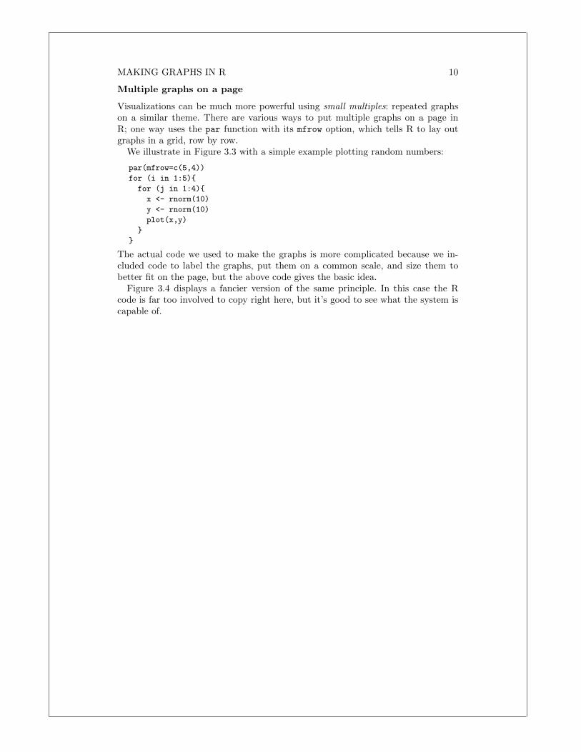
Multiple graphs on a page

Visualizations can be much more powerful using small multiples: repeated graphson a similar theme. There are various ways to put multiple graphs on a page inR; one way uses the par function with its mfrow option, which tells R to lay outgraphs in a grid, row by row.

We illustrate in Figure 3.3 with a simple example plotting random numbers:

par(mfrow=c(5,4))

for (i in 1:5){

for (j in 1:4){

x <- rnorm(10)

y <- rnorm(10)

plot(x,y)

}

}

The actual code we used to make the graphs is more complicated because we in-cluded code to label the graphs, put them on a common scale, and size them tobetter fit on the page, but the above code gives the basic idea.

Figure 3.4 displays a fancier version of the same principle. In this case the Rcode is far too involved to copy right here, but it’s good to see what the system iscapable of.

MAKING GRAPHS IN R 11

Figure 3.4 Example of a grid of graphs produced in R: estimates of public support forfederal funding for school vouchers, as a function of income, race/ethnicity/religion, andstate.

Class 4: Working with messy data in R

Reading in survey data, one question at a time

Data on the heights, weights, and incomes of a random sample of Americans areavailable from the Work, Family, and Well-Being survey conducted by CatherineRoss in 1990. We downloaded the data file, 06666-0001-Data.txt, and the code-book 06666-0001-Codebook.txt from the Inter-university Consortium for Politicaland Social Research. Information on the survey is athttp://dx.doi.org/10.3886/ICPSR06666 and can be downloaded if you createan account with the ICPSR.

We saved the files under the names wfw90.dat and wfwcodebook.txt in thedirectory http://www.stat.columbia.edu/~gelman/bda.course/.

Figure 4.1 shows the first ten lines of the data, and Figure 4.2 shows the relevantportion of the codebook. Our first step is to save the data file wfwcodebook.txt

in our working directory. We then want to extract the responses to the questionsof interest. To do this we first create a simple function, to read columns of data,making use of R’s function read.fwf (read in fixed width format).

Copy the following into the R console and then you will be able to use our functionfor reading one variable at a time from the survey. The following code is a bit trickyso you’re not expected to understand it; you can just copy it in and use it.

read.columns <- function (filename, columns) {

start <- min(columns)

length <- max(columns) - start + 1

if (start == 1)

return(read.fwf(filename, widths = length))

else

return(read.fwf(filename, widths = c(start - 1, length))[,2])

}

Now we extract the data that we are interested in.

height_feet <- read.columns("wfw90.dat", 144)

height_inches <- read.columns("wfw90.dat", 145:146)

weight <- read.columns("wfw90.dat", 147:149)

income_exact <- read.columns("wfw90.dat", 203:208)

income_approx <- read.columns("wfw90.dat", 209:210)

sex <- read.columns("wfw90.dat", 219)

100022 31659123 121222113121432 22 2 3 411179797979797 1 4 503100100...100081 486 2122 111222141122221222 2 1 997979797979797 1 4 01 25 25...100091 1371123 1232122111113111314 1 0 30100...100101 15684222 133122121113232 22 1 0 10 40...100111 25371122 122222111111421222 2 2 4 6979797979797 1 2 853 30 95...100202 2389013 1111221412 22 314 2 0 100100...100281 7884021 2232132422 42 22 2 0 80 60...100351 15684221 233223242112212 32 2 0 75100...100571 88341221 243233321113452 12 2 0 90 98...100641 15684223 122112211113432 22 2 0 100 75...

Figure 4.1 First ten lines of the file wfw90.dat, which has data from the Work, Family,and Well-Being survey.

12

WORKING WITH MESSY DATA IN R 13

HEIGHT 144-146 F3.0 Q.46 HEIGHT IN INCHES

WEIGHT 147-149 F3.0 Q.47 WEIGHT

. . .

EARN1 203-208 F6.0 Q.61 PERSONAL INCOME - EXACT AMOUNT

EARN2 209-210 F2.0 Q.61 PERSONAL INCOME - APPROXIMATION

SEX 219 F1.0 Q.63 GENDER OF RESPONDENT

. . .

HEIGHT

46. What is your height without shoes on?

__________ ft. __________in.

WEIGHT

47. What is your weight without clothing?

__________ lbs.

. . .

61a. During 1989, what was your personal income from your own wages,

salary, or other sources, before taxes?

EARN1

$ __________--> (SKIP TO Q-62a)

DON’T KNOW . . . 98

REFUSED . . . . 99

Figure 4.2 Selected rows of the file wfwcodebook.txt, which first identifies the columns inthe data corresponding to each survey question and then gives the question wordings.

The data did not come in a convenient comma-separated or tab-separated format,so we used the function read.columns to read the coded responses, one questionat a time.

Cleaning data within R

We now must put the data together in a useful form, doing the following for eachvariable of interest:

1. Look at the data

2. Identify errors or missing data

3. Transform or combine raw data into summaries of interest.

We start with height, typing: table(height_feet, height_inches). Here isthe result:

height.feet 0 1 2 3 4 5 6 7 8 9 10 11 98 99

4 0 0 0 0 0 0 0 0 0 1 3 17 0 0

5 66 56 144 173 250 155 247 127 174 105 145 90 0 0

6 129 59 46 20 8 5 1 0 0 0 1 0 0 0

7 0 0 0 0 0 0 0 1 0 0 0 0 0 0

9 0 0 0 0 0 0 0 0 0 0 0 0 2 6

Most of the data look fine, but there are some people with 9 feet and 98 or 99inches (missing data codes) and one person who is 7 feet 7 inches tall (probably adata error). We recode these problem cases as missing:

height_inches[height_inches>11] <- NA

height_feet[height_feet>=7] <- NA

And then we define a combined height variable:

height <- 12*height_feet + height_inches

We do the same thing for sex:

WORKING WITH MESSY DATA IN R 14

table(sex)

which simply yields:

sex

1 2

749 1282

No problems. But we prefer to have a more descriptive name, so we define a newvariable, female:

female <- sex - 1

This indicator variable equals 0 for men and one for women.Next, we type table(weight) and get the following:

weight

80 85 87 89 90 92 93 95 96 98 99 100 102 103 104 105 106 107 108 110

1 1 1 1 1 1 1 2 2 3 1 12 5 4 3 16 1 5 7 46

111 112 113 114 115 116 117 118 119 120 121 122 123 124 125 126 127 128 129 130

4 15 5 5 42 5 4 21 4 72 4 14 20 11 61 11 3 25 8 106

131 132 133 134 135 136 137 138 139 140 141 142 143 144 145 146 147 148 149 150

4 16 9 5 85 9 10 15 4 94 1 12 2 4 74 2 7 8 5 121

151 152 153 154 155 156 157 158 159 160 161 162 163 164 165 166 167 168 169 170

2 4 8 7 49 3 6 14 1 88 1 8 4 9 65 2 2 8 2 81

171 172 173 174 175 176 178 180 181 182 183 184 185 186 187 188 189 190 192 193

2 10 4 2 58 5 4 78 3 4 2 4 62 1 5 1 3 46 1 3

194 195 196 197 198 199 200 201 202 203 205 206 207 208 209 210 211 212 214 215

4 26 3 2 3 2 57 1 2 2 11 2 3 2 3 36 1 2 3 10

217 218 219 220 221 222 223 225 228 230 231 235 237 240 241 244 248 250 255 256

1 1 1 21 2 1 1 13 2 17 1 3 1 13 1 1 1 10 3 1

260 265 268 270 275 280 295 312 342 998 999

2 3 1 3 1 3 1 1 1 6 36

Everything looks fine until the end. 998 and 999 must be missing data, which weduly code as such:

weight[weight>500] <- NA

Coding the income responses is more complicated. The variable income_exact

contains exact responses for income (in dollars per year) for those who answered thequestion. Typing table(is.na(income_exact)) reveals that 1380 people answeredthe question (that is, is.na(income_exact) is FALSE for these respondents), and651 did not answer (is.na was TRUE). These nonrespondents were asked the second,discrete income question, income_approx, which gives incomes in round numbers(in thousands of dollars per year) for people who were willing to answer in this way.A careful look at the codebook reveals that an income_approx code of 1 corre-sponds to people who did not supply an exact income value but did say it was morethan $100,000. We code these people as having incomes of 150,000. (This is approxi-mately the average income of the over-100,000 group from the exact income data, ascalculated by mean(income_exact[income_exact>100000],na.rm=TRUE), whichyields the value 166,600.) The income_approx codes also appears to have severalvalues indicating ambiguity or missingness, which we code as NA.

We create a combined income variable as follows:

income_approx[income_approx>=90] <- NA

income_approx[income_approx==1] <- 150

income <- ifelse(is.na(income_exact), 1000*income_approx, income_exact)

The new income variable still has 237 missing values (out of 2031 respondents intotal) and is imperfect in various ways, but we have to make some choices whenworking with real data.

WORKING WITH MESSY DATA IN R 15

Looking at the data

If you stare at the table of responses to the weight question you can see more.People usually round their weight to the nearest 5 or 10 pounds, and so we see alot of weights reported as 100, 105, 110, and so forth, but not so many in between.Beyond this, people appear to like round numbers: 57 people report weights of 200pounds, compared to only 46 and 36 people reporting 190 and 210, respectively.

Similarly, if we go back to reported heights we see some evidence that the reportednumbers do not correspond exactly to physical heights: 129 people report heightsof exactly 6 feet, compared to 90 people at 5 feet 11 inches and 59 people at 6 feet1 inch. Who are these people? Let’s look at the breakdown of height and sex:

table(female, height)

Here’s the result:

height

female 57 58 59 60 61 62 63 64 65 66 67 68 69 70 71 72 73 74

0 0 0 0 3 2 4 3 14 13 47 43 81 77 119 82 125 56 44

1 1 3 17 63 54 140 170 236 142 200 84 93 28 26 8 4 3 2

height

female 75 76 77 78 82

0 19 8 5 1 1

1 1 0 0 0 0

The extra 6-footers (72 inches tall) are just about all men. But there appear to betoo many women of exactly 5 feet tall and an excess of both men and women whoreport being exactly 5 feet 6 inches.

Class 5: Some programming in R

Working with vectors

In R, a vector is a list of items. These items can include numerics, characters, orlogicals. A single value is actually represented as a vector with one element. Hereare some vectors:

• (1, 2, 3, 4, 5)

• (3, 4, 1, 1, 1)

• (“A”, “B”, “C”)

Here’s the R code to create these:

x <- 1:5

y <- c(3, 4, 1, 1, 1)

z <- c("A", "B", "C")

And here’s a random vector of 5 random numbers between 0 and 100:

u <- runif(5, 0, 100)

Mathematical operations on vectors are done componentwise. Take a look:

x

y

x + y

1000*x + u

There are scalar operations on vectors:

1 + x

2 * x

x / 3

x^4

We can summarize vectors in various ways, including the sum and the average(called the “mean” in statistics jargon):

sum(x)

mean(x)

We can also compute weighted averages if we know the weights. We illustrate witha vector of 3 elements:

x <- c(100, 200, 600)

w1 <- c(1/3, 1/3, 1/3)

w2 <- c(0.5, 0.2, 0.3)

In the above code, the vector of weights w1 has the effect of counting each of thethree items equally; vector w2 counts the first item more. Here are the weightedaverages:

sum(w1*x)

sum(w2*x)

Or suppose we want to weight in proportion to population:

N <- c(310e6, 112e6, 34e6)

sum(N*x)/sum(N)

Or, equivalently,

16

SOME PROGRAMMING IN R 17

N <- c(310e6, 112e6, 34e6)

w <- N/sum(N)

sum(w*x)

The cumsum() function does the cumulative sum. Try this:

a <- c(1, 1, 1, 1, 1)

cumsum(a)

a <- c(2, 4, 6, 8, 10)

cumsum(a)

Subscripting

Vectors can be indexed by using brackets, “[ ]”. Within the brackets we can putin a vector of elements we are interested in either as a vector of numbers or a logicalvector. When using a vector of numbers, the vector can be arbitrary length, butwhen indexing using a logical vector, the length of the vector must match the lengthof the vector you are indexing. Try these:

a <- c("A", "B", "C", "D", "E", "F", "G", "H", "I", "J")

a[1]

a[2]

a[4:6]

a[c(1,3,5)]

a[c(8,1:3,2)]

a[c(FALSE, FALSE, FALSE, TRUE, TRUE, TRUE, FALSE, FALSE, FALSE, FALSE)]

As we have seen in some of the previous examples, we can perform mathematicaloperations on vectors. These vectors have to be the same length, however. If thevectors are not the same length, we can subset the vectors so they are compatible.Try these:

x <- c(1, 1, 1, 2, 2)

y <- c(2, 4, 6)

x[1:3] + y

x[3:5] * y

y[3]^x[4]

x + y

The last line runs but produces a warning. These warnings should not be ignoredsince it isn’t guaranteed that R would carry out the operation as you intended.

Writing your own functions

You can write your own function. Most of the functions we will be writing willtake in one or more vectors and return a vector. Below is an example of a simplefunction that triples the value provided:

triple <- function(x) {

return(3*x)

}

For example, to call this function, type triple(c(1,2,3,5)). This function has oneargument, x. The body of the function is within the curly braces and the argumentsof the function are available for use within the braces. In our example function, wemultiply x by 3 and we return it back to the user. If we wanted to have more thanone argument, we could do something like this:

new_function <- function(x,y,a,b) {

return(a*x+b*y)

}

SOME PROGRAMMING IN R 18

−2 −1 0 1 2 3 4 5

−10

010

20

x15

+ 1

0 *

x −

2 *

x^2

Figure 5.1 The parabola y = 15+10x−2x2, plotted in R using curve(15 + 10*x - 2*x^2,

from=-2, to=5). The maximum is at x = 2.5.

Optimization

Finding the peak of a parabola. Figure 5.1 shows the parabola y = 15 + 10x−2x2.As you can see, the peak is at x = 2.5. How can we find this solution systematically(and without using calculus, which would be cheating)? Finding the maximum ofa function is called an optimization problem. Here’s how we do it in R.

1. Graph the function, in this case, curve(15+10*x-2*x^2,from= ,to= ), whereare numbers. Play around with the “from” and “to” arguments until the max-

imum appears.

2. Write it as a function in R:

parabola <- function(x) {

return(15 + 10*x - 2*x^2)

}

3. Call optimize(). We can find the maximum of a function in R through theoptimize() function which takes the function to optimize as the first argument,the interval to optimize over as the second argument, and an optional argumentindicating whether or not you are searching for the function’s maximum. Forthe example above, suppose we are interested in maximizing over the range fromx = −100 to x = 100. Then we can call:

optimize(parabola, interval=c(-100, 100), maximum=TRUE)

This returns two values, x and f(x). The value labeled maximum is the x at whichthe function is optimized and the objective is its corresponding f(x) value.

4. Check the solution on the graph to see that it makes sense.

Restaurant pricing. Suppose you own a small restaurant and are trying to decidehow much to charge for dinner. For simplicity, suppose that dinner will have a singleprice, and that your marginal cost per dinner is $11. From a marketing survey, youhave estimated that, if you charge $x for dinner, the average number of customersper night you will get is 5000/x2. How much should you charge, if your goal is tomaximize expected net profit?

Your exepected net profit is the expected number of customers times net profitper customer; that is, (5000/x2)·(x−11). To get a sense of where this is maximized,we can first make a graph:

SOME PROGRAMMING IN R 19

net_profit <- function(x){

return((5000/x^2)*(x-11))

}

curve(net_profit(x), from=10, to=100, xlab="Price of dinner",

ylab="Net profit per night")

From a visual inspection of this curve, the peak appears to be around x = 20. Thereare two ways we can more precisely determine where net profit is maximized.

First, the brute-force approach. The optimum is clearly somewhere between 10and 100, so let’s just compute the net profit at a grid of points in this range:

x <- seq(10, 100, .1)

y <- net_profit(x)

The maximum value of net profit is then simply max(y), which equals 113.6, andwe can find the value of x where profit is maximized:

x[y==max(y)]

It turns out to be 22. (The value 22 is x[121], that is, the 122th element of x.)Above, we are subscripting the vector x with a logical vector y==max(y), which isa vector of 900 FALSE’s and one TRUE at the maximum.

We can also use the optimize() function:

optimize(net_profit, interval=c(10,100), maximum=TRUE)

The argument interval gives the range over which the optimization is computed,and we set maximum=TRUE to maximize (rather than minimize) the net profit.