Classical and Bayesian Inference in Neuroimaging: Applications

NeuroImage 16, 484–512 (2002)doi:10.1006/nimg.2002.1091, available online at http://www.idealibrary.com on

Classical and Bayesian Inference in Neuroimaging: ApplicationsK. J. Friston, D. E. Glaser, R. N. A. Henson, S. Kiebel, C. Phillips, and J. Ashburner

The Wellcome Department of Cognitive Neurology and The Institute of Cognitive Neuroscience, University College London,Queen Square, London WC1N 3BG United Kingdom

Received January 11, 2001

In Friston et al. ((2002) Neuroimage 16: 465–483) weintroduced empirical Bayes as a potentially usefulway to estimate and make inferences about effects inhierarchical models. In this paper we present a seriesof models that exemplify the diversity of problems thatcan be addressed within this framework. In hierarchi-cal linear observation models, both classical and em-pirical Bayesian approaches can be framed in terms ofcovariance component estimation (e.g., variance par-titioning). To illustrate the use of the expectation–maximization (EM) algorithm in covariance compo-nent estimation we focus first on two importantproblems in fMRI: nonsphericity induced by (i) serialor temporal correlations among errors and (ii) vari-ance components caused by the hierarchical nature ofmultisubject studies. In hierarchical observation mod-els, variance components at higher levels can be usedas constraints on the parameter estimates of lowerlevels. This enables the use of parametric empiricalBayesian (PEB) estimators, as distinct from classicalmaximum likelihood (ML) estimates. We develop thisdistinction to address: (i) The difference between re-sponse estimates based on ML and the conditionalmeans from a Bayesian approach and the implicationsfor estimates of intersubject variability. (ii) The rela-tionship between fixed- and random-effect analyses.(iii) The specificity and sensitivity of Bayesian infer-ence and, finally, (iv) the relative importance of thenumber of scans and subjects. The forgoing is con-cerned with within- and between-subject variability inmultisubject hierarchical fMRI studies. In the secondhalf of this paper we turn to Bayesian inference at thefirst (within-voxel) level, using PET data to show howpriors can be derived from the (between-voxel) distri-bution of activations over the brain. This applicationuses exactly the same ideas and formalism but, in thisinstance, the second level is provided by observationsover voxels as opposed to subjects. The ensuing poste-rior probability maps (PPMs) have enhanced anatom-ical precision and greater face validity, in relation tounderlying anatomy. Furthermore, in comparison toconventional SPMs they are not confounded by themultiple comparison problem that, in a classical con-text, dictates high thresholds and low sensitivity. We

4841053-8119/02 $35.00© 2002 Elsevier Science (USA)All rights reserved.

conclude with some general comments on Bayesianapproaches to image analysis and on some unresolvedissues. © 2002 Elsevier Science (USA)

Key Words: fMRI; PET; serial correlations; randomeffects; the EM algorithm; Bayesian inference; hierar-chical models.

INTRODUCTION

In Friston et al. (2002) we reviewed empirical Bayes-ian approaches that might find a role in neuroimaging.Empirical Bayes enables the joint estimation of anobservation model’s parameters (e.g., activations) andits hyperparameters that specify the observation’svariance components (e.g., within- and between sub-ject-variability). The estimation procedures generallyconform to EM, which, considering just the hyperpa-rameters in linear observation models, is formallyidentical to restricted maximum likelihood (ReML). Ifthere is only one variance component these iterativeschemes simplify to conventional, noniterative sum ofsquares variance estimates. However, there are manysituations when a number of hyperparameters have tobe estimated. For example, when the correlationsamong errors are unknown but can be parameterizedwith a small number of hyperparameters (c.f. serialcorrelations in fMRI time-series). Another importantexample, in fMRI, is the multisubject design in whichthe hierarchical nature of the observation induces dif-ferent variance components at each level. The aims ofthe first sections in this paper are to illustrate howvariance component estimation, with EM, can proceedin both single-level and hierarchical contexts. Second,we wanted to show how the variance components insupraordinate levels can be used to give Bayesian es-timators of effects at lower levels. In particular, theexamples emphasize that although the mechanismsinducing non-sphericity can be very different, the vari-ance component estimation problems they represent,and the analytic approaches called for, are identical.

The fMRI examples are presented in two sections. Inthe first we deal with the issue of variance componentestimation using serial correlations in single-subject

fMRI studies. In the second section we use a multisub-ject fMRI study to address intersubject variability byadding a second level to the observation model pre-sented in the first section. Endowing the model with asecond level affords the opportunity to use empiricalBayes. This enables a quantitative comparison of clas-sical and conditional single-subject response estimates.The notation and terms used in this paper follow Fris-ton et al. (2002).

1. VARIANCE COMPONENT ESTIMATIONIN fMRI: A SINGLE-LEVEL MODEL

In this section we review serial correlations in fMRIand use simulated data to compare ReML estimates,obtained with EM, to estimates of correlations basedsimply on the model residuals. The importance of mod-elling temporal correlations, for classical inferencebased on the T statistic, is discussed in terms of cor-recting for nonsphericity in fMRI time-series. This sec-tion concludes with a quantitative assessment of serialcorrelations within and between subjects.

1.1 Serial Correlations in fMRI

In this section we restrict ourselves to a single-levelmodel and focus on the covariance component estima-tion offered by the EM algorithm. We have elected touse an important covariance estimation problem toillustrate one of the potential uses of the scheme de-scribed in Friston et al. (2002). Namely serial correla-tions in fMRI embodied in the error covariance matrixfor the first (and only) level of this observation modelC�

(1) (as in the previous paper the superscript signifiesthe hierarchical level in question). Serial correlationshave a long history in the analysis of fMRI time-seriesand are still the subject of current work: fMRI time-series can be viewed as a linear admixture of signaland noise. Signal corresponds to neuronally mediatedhemodynamic changes that can be modeled as a [non-]linear convolution of some underlying neuronal or syn-aptic process, responding to changes in experimentalfactors, by a hemodynamic response functions (HRF).Noise has many contributions that render it rathercomplicated in relation to other neurophysiologicalmeasurements. These include neuronal and nonneuro-nal sources. Neuronal noise refers to neurogenic signalnot modeled by the explanatory variables and has thesame frequency structure as the signal itself. Nonneu-ronal components have both white (e.g., R.F. noise) andcolored components (e.g., pulsatile motion of the braincaused by cardiac cycles and local modulation of thestatic magnetic field B0 by respiratory movement).These effects are typically low frequency or wide-band(e.g., aliased cardiac-locked pulsatile motion) and in-duce long range correlations in the errors over time.Currently there are two approaches to serial correla-

tions of this sort: (i) The data are filtered with a spec-ified filter to impose a known correlation structure onthe errors and are then entered into a generalized leastsquares scheme as described in Worsley and Friston(1995). (ii) The correlations are estimated, in somefashion, and these estimates are used to give minimumvariance or Gauss-Markov estimators (see Eq. (15) inFriston et al., 2002) (e.g., Purdon and Weisskoff, 1998).These are equivalent to ordinary least squares (OLS)estimators based on pre-whitened data (Bullmore etal., 1996). The second approach, in principle, is moreefficient but depends upon an accurate estimation ofthe serial correlations and inversion of the estimatedcorrelation matrix. The first approach eschews thisinversion and, more importantly, bias in the estimateof the standard error that ensues from a mismatchbetween the true and estimated correlations. However,it does so at the expense of efficiency (see Friston et al.,2000, for details). It would be nice to be estimate theserial correlations directly from the data and use theGauss–Markov estimators but there is a fundamentalproblem. In order to estimate correlations among theerrors C(�)�, in terms of some hyperparameters �, oneneeds both the residuals of the model r and the covari-ance of the parameter estimates that produced thoseresiduals. These combine to give the required errorcovariance (c.f. Eq. (A.4) in Friston et al., 2002).

C�� rr T � XC��yX T (1)

XC��yXT represents the conditional covariance of the

parameter estimates C��y “projected” onto the measure-ment space, by the design matrix X. The problem isthat the covariance of the parameter estimates is itselfa function of the error covariance. This circular prob-lem is solved by the recursive parameter reestimationimplicit in the EM algorithm. It is worth noting thatestimators of serial correlations based solely on theresiduals (produced by any estimator) will be biased.This bias results from ignoring the second term in (1),which accounts for the component of error covariancedue to the inherent variability of the parameter esti-mates themselves. It is likely that any valid recursivescheme for estimating serial correlations in fMRI time-series will conform to EM (or ReML) even if the con-nection is not made explicit. See Worsley et al. (2002)for a clever noniterative approach to AR(p) models.

In summary, the covariance estimation afforded byEM can be harnessed to estimate serial correlations infMRI time series that coincidentally provide the mostefficient (i.e., Gauss-Markov) estimators of the effectone is interested in. In this section we apply the EMalgorithm described in Friston et al. (2002) to simu-lated fMRI data sequences and take the opportunity toestablish the connections among some commonly em-ployed inference procedures based upon the T statistic.

485CLASSICAL AND BAYESIAN INFERENCE IN NEUROIMAGING

This section concludes with an application of EM toempirical data to demonstrate quantitatively the rela-tive variability in serial correlations over voxels andsubjects.

1.2 Estimating Serial Correlations

For each fMRI session we have a single-level obser-vation model that is specified by the design matrix X(1)

and constraints on the observation’s covariance struc-ture Qi

(1), in this case serial correlations among theerrors.

y � X �1�� 1� � � �1�

Q 1�1� � I (2)

Q 2�1� � KK T, kij � �e j�i i � j

0 i � j

y is the measured response with errors �(1) � N{0, C�(1)}.

I is the identity matrix.1 Here Q1(1) and Q2

(1) representcovariance components of C�

(1) that model a white noiseand an autoregressive AR(1) process with an AR coef-ficient of 1/e � 0.3679. Notice that this is a very simplemodel of autocorrelations; by fixing the AR coefficientthere are just two hyperparameters that allow for dif-ferent mixtures of an AR(1) process and white noise(c.f. the 3 hyperparameters needed for a full AR(1) pluswhite noise model). The AR(1) component is modeledas an exponential decay of correlations over nonzerolag.

These bases were chosen given the popularity of ARplus white noise models in fMRI (Purdon and Weiss-koff, 1998). Clearly this basis set can be extended inany fashion using Taylor expansions to model devia-tions of the AR coefficient from 1/e or indeed model anyother form of serial correlations. Nonstationary auto-correlations are modeled by using non-Toeplitz formsfor the bases that allow the elements in the diagonalsof Qi

(1) to vary over observations. This might be useful,for example, in the analysis of event-related potentials,where the temporal frequency structure of errors maychange with peristimulus time.

In the examples below the covariance constraintswere scaled to a maximum of one. This means that thesecond hyperparameter can be interpreted directly asthe covariance between one scan and the next. Thebasis set enters, along with the data, into the EMalgorithm to provide ML estimates of the parameters�(1) and ReML estimates of the hyperparameters �(1).

An example, based on simulated data, is shown inFig. 1. In this example the design matrix comprised a

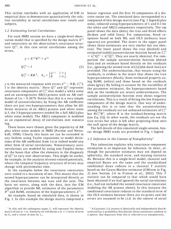
boxcar regressor and the first 16 components of a dis-crete cosine set. The simulated data corresponded to acompound of this design matrix (see Fig. 1 legend) plusnoise, coloured using hyperparameters of 1 and 0.5 forthe white and AR(1) components respectively. The toppanel shows the data (dots), the true and fitted effects(broken and solid lines). For comparison, fitted re-sponses based on both ML and OLS (ordinary leastsquares) are provided. The insert in the upper panelshows these estimators are very similar but not iden-tical. The lower panel shows the true (dashed) andestimated (solid) autocorrelation function based on C�

(1)

� �1(1)Q1

(1) � �2(1)Q2

(1). They are nearly identical. For com-parison the sample autocorrelation function (dottedline) and an estimate based directly on the residuals[i.e., ignoring the second term of (1)] (dot-dash line) areprovided. The underestimation, that ensues using theresiduals, is evident in the insert that shows the truehyperparameters (black), those estimated properly us-ing ReML (white) and those based on the residualsalone (grey). By failing to account for the variability ofthe parameter estimates, the hyperparameters basedonly on the residuals are severe underestimates. Thesample autocorrelation function even shows negativecorrelations. This is a result of fitting the low frequencycomponents of the design matrix. One way of under-standing this is to note that the autocorrelationsamong the residuals are not unbiased estimators of C�

(1)

but RC�(1)RT, where R is the residual-forming matrix

(see Eq. (5)). In other words, the residuals are not thetrue errors but what is left after projecting them ontothe null space of the design matrix.

The full details of this simulated single-session, box-car design fMRI study are provided in Fig. 1 legend.

1.3 Inference in the Context of Nonsphericity2

This subsection explains why covariance componentestimation is so important for inference. In short, al-though the parameter estimates may not depend onsphericity, the standard error, and ensuing statisticsdo. Because this is a single-level model, classical andempirical Bayes are the same and the standardizedconditional mean reduces to a classical T statisticbased on the Gauss-Markov estimator (GM/scm in Fig.2) (see Section 2.6 in Friston et al., 2002). This Tstatistic can be compared to that which would havebeen obtained if we had ignored the serial correlations(i.e., had not included the second covariance constraintmodeling the AR process above). In this instance theconditional covariance reduces to the standard error ofthe OLS estimate because there are no priors and theerrors are assumed to be i.i.d. In the context of serial

1 In this and the subsequent paper Im will represent the identitymatrix of size m � m. Similarly we will denote a m � 1 vector of zerosby 0m and a vector of ones by 1m.

2 A Gaussian i.i.d. process is identically and independently distrib-uted and has a probability distribution whose isocontours conform toa sphere. Any departure from this is referred to as nonsphericity.

486 FRISTON ET AL.

correlation’s the OLS standard error is biased, leadingto an underestimate and an inflated T value (i.i.d. inFig. 2). The difference between the two T values is dueto a departure from i.i.d. assumptions that is not ac-commodated by the OLS scheme. This departure is

referred to as nonsphericity in analysis of variance andusually calls for some nonsphericity correction.

The impact of serial correlations on inference wasnoted early in the fMRI analysis literature (Friston etal., 1994) and led to the generalized least squares

FIG. 1. Top panel: True response (an activation plus random low frequency components) and that based on the OLS and ML estimatorsfor a simulated fMRI experiment. The insert shows the similarity between the OLS and ML predictions. Lower panel: True (dashed) andestimated (solid) autocorrelation functions. The sample autocorrelation function of the residuals (dotted line) and the best fit in terms of thecovariance constraints (dot-dashed) are also shown. The insert shows the true covariance hyperparameters (black), those obtained just usingthe residuals (grey) and those estimated by the EM algorithm (white). Note, in relation to the EM estimates, those based directly on theresiduals severely underestimate the actual correlations. The simulated data comprised 128 observations with an interscan interval of 2 s.The activations were modeled with a box-car (duty cycle 64 s) convolved with a canonical hemodynamic response function and scaled to a peakheight of 2. The constant terms and low frequency components were simulated with a linear combination of the first 16 components of adiscrete cosine set, each scaled by a random unit Gaussian variate. Serially correlated noise was formed by filtering unit Gaussian noise witha convolution kernel based on covariance hyperparameters of 1.0 [uncorrelated or white component] and 0.5 [AR(1) component].


(GLS) scheme described in Worsley and Friston (1995).In this scheme one starts with any observation modelthat is premultiplied by some weighting or convolutionmatrix S to give

Sy � SX �1�� 1� � S� �1� (3)

The GLS parameter estimates and their covariance are

�LS � Ly

Cov��LS � LC ��1�L T (4)

L � �X �1�TVX �1�� 1X �1�V,

where V � STS represents the correlations induced byS. These estimators minimize the generalized leastsquare index (y � X(1)�LS)TV(y � X(1)�LS). This family ofestimators are unbiased but not necessarily ML esti-mates. The Gauss–Markov estimator is the minimumvariance and ML estimator that obtains when V �C�

(1)�1. From Eq. (3) it can be seen that this special caseis the same as whitening the data with a decorrelatingconvolution matrix and then using an OLS estimator.Usually one would use the ML estimator. However,there are some situations where a GLS estimator ismore practical. For example, when using the samedesign matrix and filtering for every voxel, the ensuingestimators are GLS if the serial correlations at each

voxel are slightly different precluding an exact MLestimate at any single voxel.3

The T statistic corresponding to the GLS estimator isdistributed with v degrees of freedom where (Worsleyand Friston, 1995)

T �c T�LS

�c TCov��LSc

v �tr�RSC �

�1�S 2

tr�RSC ��1�SRSC �

�1�S(5)

R � 1 X �1�L.

The effective degrees of freedom are based on an ap-proximation due to Satterthwaite (1941). This formu-lation is formally identical to the nonsphericity correc-tion elaborated by Box (1954), which is commonlyknown as the Geisser–Greenhouse correction in classi-cal analysis of variance, ANOVA (Geisser and Green-house, 1958). Note that in Fig. 2 the T statistic basedon the GLS estimator (WF) is slightly bigger than thestandardized conditional mean, but has a null distri-bution with fewer degrees of freedom.

The key point here is that EM can be employed togive ReML estimates of correlations among the errorsthat enter into (5) to enable classical inference, prop-erly adjusted for nonsphericity, about any GLS estima-tor. The inference is exact, to the extent that the Sat-terthwaite approximation holds, and is the basis of theGeisser–Greenhouse correction in ANOVA and v theeffective degrees of freedom in Worsley and Friston(1995). The ensuing T statistic for the simulated fMRIdata, for S � 1 (i.e., no temporal filtering), is shown inFig. 2.

EM finds a special role in enabling inferences aboutGLS estimators in statistical parametric mapping.When the relative values of hyperparameters can beassumed to be stationary over voxels, ReML estimatescan be obtained using the sample covariance of thedata over voxels, in a single EM (see Eq. (A.7) in

3 As discussed in Friston et al. (2000) the GLS scheme was origi-nally introduced to ensure robust estimates of variance in the face ofunknown serial correlations. In that paper, the hyperparameter wasestimated using the filtered residuals

� �tr�SRyyTR TS T

tr�SRQ �1�R TS T�

y TR TS TSRy

tr�RSQ �1�S

This estimate is generally more robust to misspecification of the formof serial correlations Q(1) if a suitable form for S is adopted. One mildbut obvious misspecification is when the same correlation structureis assumed for every voxel. When S � C�

�1/2 this is the ReML esti-mator (see footnote 3 in Friston et al., 2002). In Friston et al. (2000)the residual forming matrix R is related to the current notation bySR � RS.

FIG. 2. T statistics based on the simulated data of Fig. 1. Thesecorresponding to; (i) the standardized ordinary least square estima-tor under i.i.d. assumptions about the error terms (i.i.d.). The stan-dardized conditional mean which is equivalent to the standardizedGauss–Markov estimator obtained using the correlation structureestimated by the EM algorithm (GM/scm) and (iii) the standardizedgeneralized least squares estimator of Worsley and Friston (1995)using the same correlation estimate (WF). All are valid apart fromthe naive i.i.d. scheme that ignores serial correlations or non-sphe-ricity among the errors. The degrees of freedom (d.f.) are provided foreach statistic and were calculated according to (5).

488 FRISTON ET AL.

Friston et al., 2002). After renormalization, the ensu-ing estimate of the nonsphericity Q(1) � ¥ �kQk

(1) speci-fies the serial correlations in terms of a single basis.Voxel-specific hyperparameters can now be estimatedin a non-iterative fashion in the usual way, becausethere is only one hyperparameter to estimate (see foot-note 3 of Friston et al., 2002, and this paper). This isvery convenient from a computational perspective.This device is not limited to serial correlations in fMRIbut can be applied in any context where nonsphericityis an issue. We will pursue this in a subsequent paperdealing with nonsphericity correction in multistageanalyses of fMRI data.

1.4 Application to Empirical Data

In this subsection we address the variability of serialcorrelations over voxels within subject and over sub-jects within the same voxel. Here we are concernedonly with the form of the correlations (see Section2.3 for a discussion of between-subject error varianceper se).

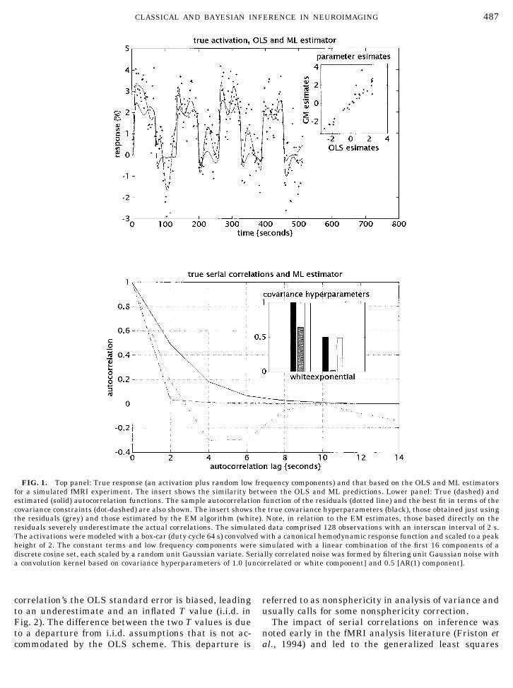
Using the model specification in (2) serial correla-tions were estimated using EM in 12 randomly selectedvoxels from the same slice from a single subject. Theresults are shown in Fig. 3 (left panel) and show thatthe correlations from one scan to the next can varybetween about 0.1 and 0.4. The data sequences andexperimental paradigm are described in the figure leg-end. Briefly these data came from an event-related

study of visual word processing in which new and oldwords (i.e., encoded during a prescanning session) werepresented in a random order with a stimulus onsetasynchrony (SOA) of about 4 s. These data will be usedagain in the next section. Although the serial correla-tions within subject vary somewhat there is an evengreater variability from subject to subject at the samevoxel. The right hand panel of Fig. 3 shows the auto-correlation functions estimated separately for 12 sub-jects at a single voxel. In this instance, the correlationsbetween one scan and the next range from about �0.1to 0.3 with a greater dispersion relative to the within-subject autocorrelations.

1.5 Summary

These results are provided to illustrate one potentialapplication of covariance component estimation, not toprovide an exhaustive characterization of serial corre-lations. This sort of application may be importantwhen it comes to making assumptions about models forserial correlations at different voxels or among sub-jects. We have chosen to focus on a covariance estima-tion problem that requires an iterative parameter re-estimation procedure in which the hyperparameterscontrolling the covariances depend on the variance ofthe parameter estimates and vice versa. There areother important applications of covariance componentestimation we could have considered (although not allrequire an iterative scheme). One example is the esti-mation of condition-specific error variances in PET andfMRI. In conventional SPM analyses one generally as-sumes that the error variance expressed in one condi-tion is the same as that in another. This represents asphericity assumption over conditions and allows oneto pool several conditions when estimating the errorvariance. Assumptions of this sort, and related sphe-ricity assumptions in multi-subject studies, can be eas-ily addressed in unbalanced designs, or even in thecontext of missing data, using EM.

2. VARIANCE COMPONENT ESTIMATIONIN fMRI: TWO-LEVEL MODELS

In this section we augment the model of the previoussection with a second level. This engenders a number ofimportant issues, including (i) the distinction betweenfixed- and random-effect inferences about the subjects’responses, (ii) the opportunity to make Bayesian infer-ences about single-subject responses and (iii) the role ofvariance component estimation in power analyses ofclassical inference at the second level. As in previoussections we start with model specification, proceed tosimulated data and conclude with an empirical exam-ple. In this section the second level represents obser-vations over subjects. Analyses of simulated data areused to illustrate the distinction between fixed- and

FIG. 3. Estimates of serial correlations expressed as autocorre-lation functions based on empirical data. Left panel: Estimates from12 randomly selected voxels from a single subject. Right panel:Estimates from the same voxel over 12 different subjects. The voxelwas in the cingulate gyrus and came from same slice reported inSection 2. The empirical data are described in Henson et al. (2000).They comprised 300 vol, acquired with EPI at two Tesla and a TR of3 s. The experimental design was stochastic and event-related look-ing for differential response evoked by new relative to old (studiedprior to the scanning session) words. Either a new or old word waspresented visually with a mean stimulus onset asynchrony (SOA) of4 s (SOA varied randomly between 2.5 and 5.5 s). Subjects wererequired to make an old vs new judgment for each word. The designmatrix for these data comprised two regressors (early and late) foreach of the four trial types (old vs new and correct vs incorrect) andthe first 16 components of a discrete cosine set (as in the simula-tions).


random-effect inferences by looking at how their re-spective T values depend on the variance componentsand design factors. The empirical analyses are used toassess, quantitatively, the sensitivity and specificity ofBayesian inference at the first level and classical in-ference at the second. The fMRI data are the same asused in section 1 and comprise event-related time-series from 12 subjects. We chose a data set that wouldbe difficult to analyze rigorously using software avail-able routinely. These data not only evidence serialcorrelations but also the number of trial-specific eventsvaried from subject to subject, giving an unbalanceddesign.

2.1 Model Specification

The observation model here comprises two levelswith the opportunity for subject-specific differences inerror variance and serial correlations at the first leveland parameter-specific variance at the second. Theestimation model here is simply an extension of thatused in the previous section to estimate serial correla-tions. Here it embodies a second level that accommo-dates observations over subjects.

level one y � X �1�� 1� � � �1�

�y1

···ys� � �

X 1�1� · · · 0···

· · ····

0 · · · X s�1��

� 1�1�

···� s

�1�� 1�

Q 1�1� � �

It · · · 0···

· · ····

0 · · · 0� , . . . , Q s

�1� � �0 · · · 0···

· · ····

0 · · · It�

Q s�1�1� � �

KK T · · · 0···

· · ····

0 · · · 0� , . . . ,

Q 2s�1� � �

0 · · · 0···

· · ····

0 · · · KK T�

(6)

level two � �1� � X �2�� 2� � � �2�

X �2� � 1s � Ip

Q 1�2� � Is � �

1 · · · 0···

· · ····

0 · · · 0� , . . . ,

Q p�2� � Is � �

0 · · · 0···

· · ····

0 · · · 1�

for s subjects each scanned on t occasions and p param-eters. The Kronecker tensor product A V B simplyreplaces the element of A with AijB. An example ofthese design matrices and covariance constraints wereshown, respectively, in Figs. 1 and 3 of Friston et al.(2002). Note that there are 2s error covariance con-straints, one set for the white noise components andone for AR(1) components. Similarly, there are asmany prior covariance constraints as there are param-eters at the second level.

2.2 Simulations

In the simulations we used 128 scans for each of 12subjects. The design matrix comprised three effects,modeling an event-related hemodynamic response tofrequent but sporadic trials (in fact the instances ofcorrectly identified “old” words from the empirical ex-ample below) and a constant term. Activations weremodeled with two regressors, constructed by convolv-ing a series of delta functions with a canonical hemo-dynamic response function (HRF)4 and the same func-tion delayed by 3 s. The delta functions indexed theoccurrence of each event. These regressors modelevent-related responses with two temporal compo-nents, which we will refer to as “early” and “late” (c.f.Henson et al., 2000). Each subject-specific design ma-trix therefore constituted three columns giving a totalof 36 parameters at the first level and three at thesecond. The HRF basis functions were scaled so that aparameter estimate of one corresponds to a peak re-sponse of unity. After division by the grand mean, andmultiplication by 100, the units of the response vari-able and parameter estimates were rendered adimen-sional and correspond to percent whole brain meanover all scans. The simulated data were generatedusing (6) with unit Gaussian noise coloured using atemporal, convolution matrix (¥ �k

(1)Qk(1))1/2 with first-

level hyperparameters �j(1) � 0.5 and �0.1 for each

subject’s white and AR(1) error covariance compo-nents, respectively. The second level parameters andhyperparameters were �(2) � [0.5, 0, 0]T, �(2) � [0.02,0.006, 0]T. These model substantial early responseswith an expected value of 0.5% and a standard devia-tion over subjects of 0.14% (i.e., square root of 0.02).The late component was trivial with zero expectationand a standard deviation of 0.077%. The third or con-stant terms were discounted with zero mean and vari-ance. These values were chosen because they are typ-ical of real data (see below).

Figures 4 and 5 show the results after entering thesimulated data into the EM algorithm to estimate

4 The canonical HRF was the same as that employed by SPM. Itcomprises a mixture of two gamma variates modeling peak andundershoot components and is based on a principal component anal-ysis of empirically determined hemodynamic responses, over voxels,as described in Friston et al. (1998).

490 FRISTON ET AL.

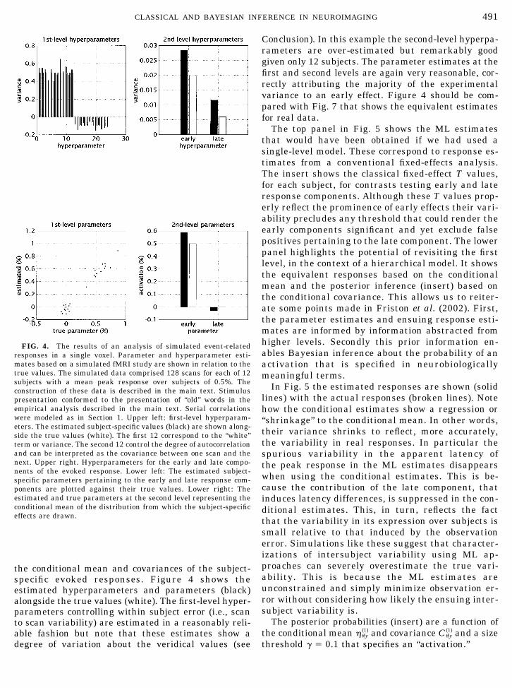
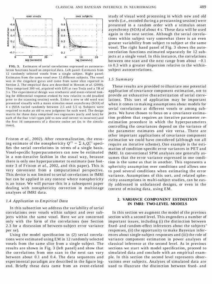
the conditional mean and covariances of the subject-specific evoked responses. Figure 4 shows theestimated hyperparameters and parameters (black)alongside the true values (white). The first-level hyper-parameters controlling within subject error (i.e., scanto scan variability) are estimated in a reasonably reli-able fashion but note that these estimates show adegree of variation about the veridical values (see

Conclusion). In this example the second-level hyperpa-rameters are over-estimated but remarkably goodgiven only 12 subjects. The parameter estimates at thefirst and second levels are again very reasonable, cor-rectly attributing the majority of the experimentalvariance to an early effect. Figure 4 should be com-pared with Fig. 7 that shows the equivalent estimatesfor real data.

The top panel in Fig. 5 shows the ML estimatesthat would have been obtained if we had used asingle-level model. These correspond to response es-timates from a conventional fixed-effects analysis.The insert shows the classical fixed-effect T values,for each subject, for contrasts testing early and lateresponse components. Although these T values prop-erly reflect the prominence of early effects their vari-ability precludes any threshold that could render theearly components significant and yet exclude falsepositives pertaining to the late component. The lowerpanel highlights the potential of revisiting the firstlevel, in the context of a hierarchical model. It showsthe equivalent responses based on the conditionalmean and the posterior inference (insert) based onthe conditional covariance. This allows us to reiter-ate some points made in Friston et al. (2002). First,the parameter estimates and ensuing response esti-mates are informed by information abstracted fromhigher levels. Secondly this prior information en-ables Bayesian inference about the probability of anactivation that is specified in neurobiologicallymeaningful terms.

In Fig. 5 the estimated responses are shown (solidlines) with the actual responses (broken lines). Notehow the conditional estimates show a regression or“shrinkage” to the conditional mean. In other words,their variance shrinks to reflect, more accurately,the variability in real responses. In particular thespurious variability in the apparent latency ofthe peak response in the ML estimates disappearswhen using the conditional estimates. This is be-cause the contribution of the late component, thatinduces latency differences, is suppressed in the con-ditional estimates. This, in turn, reflects the factthat the variability in its expression over subjects issmall relative to that induced by the observationerror. Simulations like these suggest that character-izations of intersubject variability using ML ap-proaches can severely overestimate the true vari-ability. This is because the ML estimates areunconstrained and simply minimize observation er-ror without considering how likely the ensuing inter-subject variability is.

The posterior probabilities (insert) are a function ofthe conditional mean ��y

(1) and covariance C��y(1) and a size

threshold � 0.1 that specifies an “activation.”

FIG. 4. The results of an analysis of simulated event-relatedresponses in a single voxel. Parameter and hyperparameter esti-mates based on a simulated fMRI study are shown in relation to thetrue values. The simulated data comprised 128 scans for each of 12subjects with a mean peak response over subjects of 0.5%. Theconstruction of these data is described in the main text. Stimuluspresentation conformed to the presentation of “old” words in theempirical analysis described in the main text. Serial correlationswere modeled as in Section 1. Upper left: first-level hyperparam-eters. The estimated subject-specific values (black) are shown along-side the true values (white). The first 12 correspond to the “white”term or variance. The second 12 control the degree of autocorrelationand can be interpreted as the covariance between one scan and thenext. Upper right. Hyperparameters for the early and late compo-nents of the evoked response. Lower left: The estimated subject-specific parameters pertaining to the early and late response com-ponents are plotted against their true values. Lower right: Theestimated and true parameters at the second level representing theconditional mean of the distribution from which the subject-specificeffects are drawn.


1 � c jT� ��y

�1�

�c jTC ��y

�1�cj� (7)

The contrast weight vectors were cearly � [1, 0, 0]T andclate � [0, 1, 0]T. As expected, the probability of the early

response component being greater than was uni-formly high for all 12 subjects, whereas the equivalentprobability for the late component was negligible. Notethat, in contradistinction to the classical inference,there is now a clear indication that each subject ex-pressed an early response but no late response.

FIG. 5. Response estimates and inferences about the estimates described in the legend of Fig. 4: Upper panel: True (dotted) and ML(solid) estimates of event-related responses to a stimulus over 12 subjects. The units of activation are adimensional and correspond to percentof whole brain mean. The insert shows the corresponding subject-specific T values for contrasts testing for early and late responses. Lowerpanel: The equivalent estimates based on the conditional means. It can be seen that the conditional estimates are much “tighter” and reflectbetter the intersubject variability in responses. The insert shows the posterior probability that the activation was greater than 0.1%. Becausethe responses were modeled with early and late components (basis functions corresponding to canonical hemodynamic response functions,separated by 3 s) separate posterior probabilities could be computed for each. The simulated data comprised only early responses as reflectedin the posterior probabilities.

492 FRISTON ET AL.

2.3 Classical Fixed- and Random-Effect Analyses

In this subsection we focus on the importance ofcovariance component estimation from a classical per-spective, in particular the differences in classical infer-ence using fixed (single-level) and random (two-level)effect analyses. In this two-level model the variancepartitioning is

E�yy T � C ��1�

error

� X �1�C ��2�X �1�T

2nd-level random effects

� X �1�X �2�� 2�� 2�TX �2�TX �1�T

fixed effects

(8)

The first term on the right is simply observation error.The second term corresponds to variance in the re-sponse variable due to between-subject variability inthe parameters that is projected down to the observa-tion space by the first-level design matrix. The finalterm corresponds to the sum of squares due the fixedeffects at the second level (i.e., the mean effects oversubjects) projected down by the design matrices at bothlevels. Observation error corresponds to within-subjecterror, second-level random effects correspond to be-tween-subject error and the fixed effects to the vari-ance attributable to activations per se.

What implications does this variance partitioninghave for the classical inference? Recall from equation(9) in Friston et al. (2002) that the T statistic can beexpressed in terms of error variances at all levels spec-ified. For this two-level model the random effects Tstatistic is

T �2� � c TM �2�y/�c TM �2�C �̃M �2�Tc(9)

C �̃ � C ��1� � X �1�C �

�2�X �1�T,

where M(2) is the ML projector as defined in (7) inFriston et al. (2002). The second expression is the com-bined error in the observation that contributes to thestandard error of the contrast. It comprises within-subject error and between-subject error projected bythe first-level design matrix onto the observation space(i.e., random effects). Their relative contributions tothe standard error of the T statistic can be understoodin terms of the difference between random and fixed-effect inference in classical analyses:

Pretend that we had only specified our model to thefirst level. To test for the mean activation we wouldhave to augment c to average over subjects givingc(1)T � cTX(2)� (� denotes pseudoinverse). Here the sec-ond-level design matrix enters, not as a constraint onthe parameter expectations but directly into the con-trast at the first level. The corresponding fixed effects Tstatistic is

T �1� � c TX �2��M �1�y/�c TX �2��M �1�C �̃M �1�TX �2��Tc(10)

C �̃ � C ��1�.

For balanced designs with equal variances, X(2)�M(1) �M(2). In this case the only difference between the two Tstatistics is the contribution of the random effectsX(1)C�

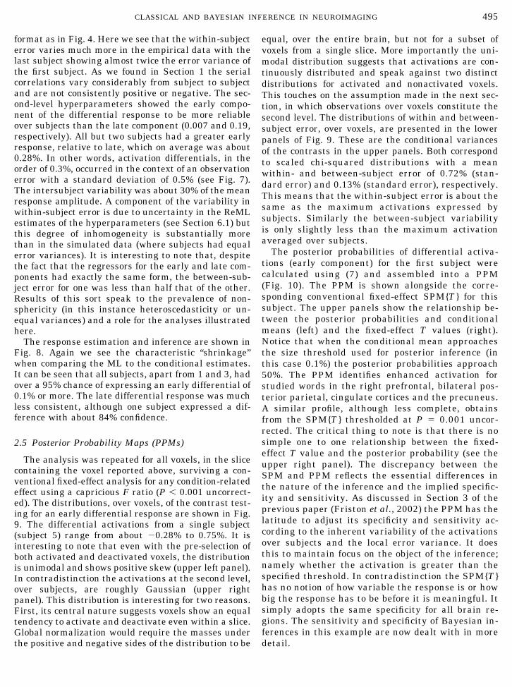
(2)X(1)T to the standard error. This contribution willbe large when (i) the second-level error is big or (ii)when the first-level design matrix amplifies its projec-tion onto the observation space, i.e., many observationsat the first level, relative to the second. This accountsfor the well-known fact that the distinction betweenthe fixed and random-effect T statistics is greater whenthe within-subject error is small relative to between-subject error and when there are many repeated mea-sures per subject. This is why random effect analysesare more critical in fMRI than in PET. In fMRI thescan to scan variability is much smaller than in PETand typically there are many more scans per session infMRI.

These points are illustrated in Fig. 6 where the Tstatistics were computed according to (9) and (10) us-ing the estimated parameters and hyperparametersfrom the simulation. In the upper panel the first-leveldesign matrix was decimated to reduce the number ofscans per subject. It can be seen that at around 16scans the fixed (broken line) and random-effect (solidline) T statistics converge, whereas there is a substan-tial difference by 32 scans. In the lower panel the errorcovariance was scaled while keeping the design matri-ces constant. In this illustration, as the error covari-ance falls to zero the fixed-effect T statistic tends toinfinity whereas the random-effect T statistic properlyreflects the intrinsic between-subject variability.

In summary, covariance component estimation iscritical for inference in hierarchical models becausemixtures of variance components are required to com-pute the standard error of contrasts. In random-effectanalyses intersubject differences are treated as a vari-ance component, rendering the inference about acontrast of effects relative to that contrast’s inherentvariability. In fixed-effect analyses this variancecomponent is discounted and the inference is in rela-tion to the precision with which the effect can be mea-sured.

2.4 Empirical Analyses

Here the analysis is repeated using real data and theresults compared to those obtained using simulateddata. We focus first on the parameter and hyperparam-eter estimates and how these are used to form posteriorprobability maps or PPMs. We then use the covariancecomponent estimates to quantify the specificity andsensitivity of Bayesian inference at the first level, andclassical inference at the second. The empirical data


are described in Henson et al. (2000). Briefly, theycomprised 128� scans in 12 subjects. Only the first 128scans were used below. The experimental design wasstochastic and event-related, looking for differentialresponses evoked by new relative to old (studied priorto the scanning session) words. Either a new or oldword was presented every 4 s or so (SOA varied be-tween 2.5 and 5.5 s). In this design one is interestedonly in the differences between evoked responses to thetwo stimulus types. This is because the efficiency of thedesign to detect the effect of stimuli per se is negligiblewith such a short SOA. Subjects were required to makean old vs. new judgment for each word. Drift (the first

8 components of a discrete cosine set) and the effects ofincorrect trials were treated as confounds and wereremoved using linear regression.5 The first-level sub-ject-specific design matrix partitions comprised fourregressors with early and late effects for both old andnew words.

The analyses proceeded in exactly the same way asfor the simulated data. The only difference was thatthe contrast tested for differences between the twoword types (i.e., c � [1, 0, �1, 0]T for an old minus newearly effect). The hyperparameter and parameter esti-mates, for a voxel in the cingulate gyrus (BA 31; �3,�33, 39 mm), are shown in Fig. 7, adopting the same

5 Strictly speaking the projection matrix implementing this adjust-ment should also be applied to the covariance constraints but thiswould (i) render the constraints singular and (ii) ruin their sparsitystructure. We therefore omitted this and ensured, in simulations,that the adjustment had a negligible effect on the hyperparameterestimates.

FIG. 6. Comparison of fixed and random-effect T values. Upperpanel: The relationship between the T values based on a single-level(FFX—broken line) and two-level hierarchical model (RFX—solidline) as a function of the number of scans for each subject’s session.Lower panel: Equivalent relationship as a function of relative with-in-subject error (the dashed vertical line corresponds to the errorestimated empirically). In the limit of high within-subject error, orvariability in its estimate due to a small number of scans the two Tstatistics converge. These results used the hyperparameter esti-mates from the analysis of the simulated data described in thelegend of Fig. 4.

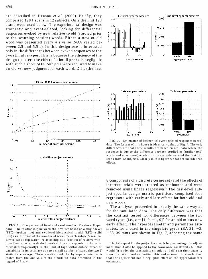
FIG. 7. Estimation of differential event-related responses in realdata. The format of this figure is identical to that of Fig. 4. The onlydifferences are that these results are based on real data where theresponse is due to the difference between studied or familiar (old)words and novel (new) words. In this example we used the first 128scans from 12 subjects. Clearly in this figure we cannot include trueeffects.

494 FRISTON ET AL.

format as in Fig. 4. Here we see that the within-subjecterror varies much more in the empirical data with thelast subject showing almost twice the error variance ofthe first subject. As we found in Section 1 the serialcorrelations vary considerably from subject to subjectand are not consistently positive or negative. The sec-ond-level hyperparameters showed the early compo-nent of the differential response to be more reliableover subjects than the late component (0.007 and 0.19,respectively). All but two subjects had a greater earlyresponse, relative to late, which on average was about0.28%. In other words, activation differentials, in theorder of 0.3%, occurred in the context of an observationerror with a standard deviation of 0.5% (see Fig. 7).The intersubject variability was about 30% of the meanresponse amplitude. A component of the variability inwithin-subject error is due to uncertainty in the ReMLestimates of the hyperparameters (see Section 6.1) butthis degree of inhomogeneity is substantially morethan in the simulated data (where subjects had equalerror variances). It is interesting to note that, despitethe fact that the regressors for the early and late com-ponents had exactly the same form, the between-sub-ject error for one was less than half that of the other.Results of this sort speak to the prevalence of non-sphericity (in this instance heteroscedasticity or un-equal variances) and a role for the analyses illustratedhere.

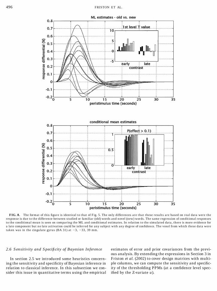
The response estimation and inference are shown inFig. 8. Again we see the characteristic “shrinkage”when comparing the ML to the conditional estimates.It can be seen that all subjects, apart from 1 and 3, hadover a 95% chance of expressing an early differential of0.1% or more. The late differential response was muchless consistent, although one subject expressed a dif-ference with about 84% confidence.

2.5 Posterior Probability Maps (PPMs)

The analysis was repeated for all voxels, in the slicecontaining the voxel reported above, surviving a con-ventional fixed-effect analysis for any condition-relatedeffect using a capricious F ratio (P � 0.001 uncorrect-ed). The distributions, over voxels, of the contrast test-ing for an early differential response are shown in Fig.9. The differential activations from a single subject(subject 5) range from about �0.28% to 0.75%. It isinteresting to note that even with the pre-selection ofboth activated and deactivated voxels, the distributionis unimodal and shows positive skew (upper left panel).In contradistinction the activations at the second level,over subjects, are roughly Gaussian (upper rightpanel). This distribution is interesting for two reasons.First, its central nature suggests voxels show an equaltendency to activate and deactivate even within a slice.Global normalization would require the masses underthe positive and negative sides of the distribution to be

equal, over the entire brain, but not for a subset ofvoxels from a single slice. More importantly the uni-modal distribution suggests that activations are con-tinuously distributed and speak against two distinctdistributions for activated and nonactivated voxels.This touches on the assumption made in the next sec-tion, in which observations over voxels constitute thesecond level. The distributions of within and between-subject error, over voxels, are presented in the lowerpanels of Fig. 9. These are the conditional variancesof the contrasts in the upper panels. Both correspondto scaled chi-squared distributions with a meanwithin- and between-subject error of 0.72% (stan-dard error) and 0.13% (standard error), respectively.This means that the within-subject error is about thesame as the maximum activations expressed bysubjects. Similarly the between-subject variabilityis only slightly less than the maximum activationaveraged over subjects.

The posterior probabilities of differential activa-tions (early component) for the first subject werecalculated using (7) and assembled into a PPM(Fig. 10). The PPM is shown alongside the corre-sponding conventional fixed-effect SPM{T} for thissubject. The upper panels show the relationship be-tween the posterior probabilities and conditionalmeans (left) and the fixed-effect T values (right).Notice that when the conditional mean approachesthe size threshold used for posterior inference (inthis case 0.1%) the posterior probabilities approach50%. The PPM identifies enhanced activation forstudied words in the right prefrontal, bilateral pos-terior parietal, cingulate cortices and the precuneus.A similar profile, although less complete, obtainsfrom the SPM{T} thresholded at P � 0.001 uncor-rected. The critical thing to note is that there is nosimple one to one relationship between the fixed-effect T value and the posterior probability (see theupper right panel). The discrepancy between theSPM and PPM reflects the essential differences inthe nature of the inference and the implied specific-ity and sensitivity. As discussed in Section 3 of theprevious paper (Friston et al., 2002) the PPM has thelatitude to adjust its specificity and sensitivity ac-cording to the inherent variability of the activationsover subjects and the local error variance. It doesthis to maintain focus on the object of the inference;namely whether the activation is greater than thespecified threshold. In contradistinction the SPM{T}has no notion of how variable the response is or howbig the response has to be before it is meaningful. Itsimply adopts the same specificity for all brain re-gions. The sensitivity and specificity of Bayesian in-ferences in this example are now dealt with in moredetail.


2.6 Sensitivity and Specificity of Bayesian Inference

In section 2.5 we introduced some heuristics concern-ing the sensitivity and specificity of Bayesian inference inrelation to classical inference. In this subsection we con-sider this issue in quantitative terms using the empirical

estimates of error and prior covariances from the previ-ous analysis. By extending the expressions in Section 3 inFriston et al. (2002) to cover design matrices with multi-ple columns, we can compute the sensitivity and specific-ity of the thresholding PPMs (at a confidence level spec-ified by the Z-variate u).

FIG. 8. The format of this figure is identical to that of Fig. 5. The only differences are that these results are based on real data were theresponse is due to the difference between studied or familiar (old) words and novel (new) words. The same regression of conditional responsesto the conditional mean is seen on comparing the ML and conditional estimates. In relation to the simulated data, there is more evidence fora late component but no late activation could be inferred for any subject with any degree of confidence. The voxel from which these data weretaken was in the cingulate gyrus (BA 31) at �3, �33, 39 mm.

496 FRISTON ET AL.

� � 1 �w�

� � 1 �w c TC��yX TC �

�1XA

�c TC�c� (11)

w � � u�c TC��yc

�c TC�c

Here the contrast weights c were chosen to test forearly activation differentials in the first subject, at thecingulate voxel reported above. Superscripts have beendropped from (11) because these expressions hold forany level considered. Here we are dealing with Bayes-ian inference at the first level. Both sensitivity andspecificity are functions of the size threshold speci-fied, whereas only sensitivity is a function of A, thetrue effect. Figure 11 shows the sensitivity or power �(solid line) and false positive rate � � 1 � specificity(broken line) as functions of the size threshold. Theseresults are for 90% confidence, given a true activationof 0.5% (vertical line). As one might expect both powerand false positive rate increase as the threshold isreduced. The lower panel shows the same relationshipbut on a semilog scale. It can be seen that false positiverate approaches very small levels as the threshold ap-proaches the true activation. In the example shown, avoxel would be correctly declared as activating by 0.1%or more on about 50% of occasions while retainingconsiderable specificity (� � 10�4). Conversely we canexamine sensitivity and specificity as functions of thetrue activation for a fixed size threshold. Figure 12shows the results for a threshold that maintains a lowfalse positive rate of � � 10�4 (vertical line). Specificityis not a function of the true activation but sensitivityincreases dramatically with activations above 0.4%.

Finally, we demonstrate the dependence on errorvariance. This is interesting because different errorvariances in different brain regions imply that Bayes-ian inference has a self-adjusting sensitivity and spec-ificity depending on the local noise. Figure 13 showspower and false positive rate as functions of relativeerror variance, modeled by scaling the error covariancebetween 0 and 4 while holding the true activation andthreshold fixed. For relatively large errors, sensitivityand false positive rate fall in tandem with increasingerror. However, the critical thing to note is that theproportional difference between the power and falsepositive rate in the semilog plot (lower panel) decreaseswith relative error variance. This means that thepower, relative to false positive rate falls more slowlywith increasing error. In other words, the balance be-tween specificity and sensitivity is implicitly adjusteddepending on the reliability of the measured response.

2.7 Sensitivity and Specificity of Classical Inference

In this final subsection we turn to inference atthe final level using the ML estimator and the Tstatistic. The aim here is to demonstrate how thecovariance component estimation can be useful froma purely classical perspective. We do this by usingthe variance partitioning to evaluate how the sensi-tivity of a classical second-level inference depends onthe relative number of subjects and scans. We cre-ated a series of synthetic balanced designs in which

FIG. 9. Results from an analyses over multiple voxels selected onthe basis of a conventional SPM analysis (F test for all event-relatedresponses, P � 0.001, uncorrected) at z � 39 mm. Upper left panel:Distribution of a contrast of conditional mean responses, here the dif-ferential peak response evoked by old words relative to new, in terms ofthe early component. This distribution is for subject 5. The noncentralnature and skew of this distribution suggests that regional responses inthis part of the brain tend to be greater for “old” relative to “new” words.However, relative deactivations are nearly as prevalent. A reasonabledifferential activation, in this context would be about 0.2%. Upper rightpanel: Equivalent contrast at the second level reflecting conditionalresponses averaged over subjects. Lower left panel: Distribution ofwithin-subject error over the same voxels. This corresponds to theconditional variance of this subject-specific contrast. The average stan-dard deviation of this error is 0.72%. Therefore responses of about 0.3%are occurring in the context of errors that are over twice their magni-tude. Lower panel: Between-subject error over the same voxels. Thisrepresents the variability in responses over subjects. It can be seen thatthe average standard deviation (0.13%) is a little less than the magni-tude of the larger responses themselves. These results are interestingbecause they frame, quantitatively the size of responses in relation tothe within-session noise and their variability over subjects.


FIG. 10. Posterior probability map (PPM) and SPM{T} pertaining to first-level effects. The posterior probability of an early differentialresponse in subject 5 was computed for the voxels described in the legend of Fig. 9. Upper panels: Posterior probability that the differentialeffects were greater than 0.1% expressed as a function of the conditional means (left) and fixed-effect T values (right). Lower panels (left).Posterior probability map (PPM) (above) and thresholded (below) to show regions that evidenced a differential peak response of 0.1% or morewith 90% confidence, or more. Lower panels (right). Equivalent SPM{T} based on the single-level model, fixed-effects T values. The thresholdadopted here (lower right panel) was 0.001 uncorrected. It can be seen that this particular subject shows quite an extensive differentialresponse involving cingulate, right prefrontal, and bilateral parietal cortices that is similar to, but more complete than, the activation profileinferred on the basis of the SPM{T} (even with this liberal threshold).

498 FRISTON ET AL.

subject-specific responses were modeled by the samedesign matrix (that of the first subject). Differentnumbers of scans per subject and numbers of sub-jects were modeled by decimating the first- and sec-ond-level design matrices, respectively. These designmatrices and the covariance hyperparameters, forthe voxel of the previous subsection, were enteredinto (9) to give the standard error of the second-levelML contrast testing for an early activation differen-tial. The sensitivity of the corresponding T test issimply

� � 1 T�w A

�c TM �2�C �̃M �2�Tc� , (12)

where w is some T value threshold and A is the trueactivation, here set to 0.001 and 0.5% respectively. Theresults are shown in Fig. 14. As might be anticipatedthere is a trade-off between the number of subjects andnumber of scans per subject. The minimum number ofsubjects, required to attain 90% sensitivity for voxelssuch as the one chosen, appears to be about 8 and thisrequires about 100 scans per subject. Scanning 16 sub-jects with about 24 scans each can approximate thesame sensitivity. This power analysis is presented asan illustration of how covariance component estima-tion can be used in a classical power analysis. Thequantitative conclusions pertain to, and only to thevoxel reported.

FIG. 12. As for Fig. 11 but holding the threshold constant atabout 0.14% (such that the specificity was at least 1 � 10�4) andvarying the true activation. In this case the specificity is constant butsensitivity increases as the true activation exceeds the specifiedthreshold.

FIG. 11. Specificity and sensitivity of first-level inferences as afunction of activation threshold: Upper panel: The probability ofdeclaring a voxel “activated” to degree u or more, with 90% confi-dence in the context of no activation (broken curve) and with a trueactivation of 0.5% (solid curve and vertical dashed line). These prob-abilities are based on the hyperparameters from the analysis ofsection 2.4. In this instance the posterior probabilities pertain to theactivations in the cingulate gyrus voxel described in the legend ofFig. 7, in the first subject. Lower panel: The same as in the upperpanel but plotted on a semilog scale. A 50% sensitivity is achievedwith an activation threshold of about 0.1% whilst retaining a highspecificity.


2.8 Summary

The examples presented above allow us to reprise anumber of important points made in the previous pa-per (Friston et al., 2002). In conclusion the main pointsare:

● There are many instances when an iterative pa-rameter re-estimation scheme is required (e.g., dealingwith serial correlations or missing data). Theseschemes are generally variants of an EM algorithm.

● Even before considering the central role of covari-ance component estimation in hierarchical or empiricalBayes models it is an important aspect of model esti-mation in its own right, particularly in estimating non-sphericity among observation errors. Parameter esti-

mates can either be obtained directly from an EMalgorithm, in which case they correspond to the ML orGauss–Markov estimates, or the hyperparameterscan be used to determine the error correlations whichreenter a generalized least square scheme, as a non-sphericity correction.

● Hierarchical models enable a collective improve-ment in response estimates by using conditional, asopposed to maximum-likelihood, estimators. This im-provement ensues from the constraints derived fromhigher levels that enter as priors at lower levels.

● The sensitivity and specificity of Bayesian infer-ence differs from that of classical approaches. In par-ticular, Bayesian inference maintains a high specificitywhile adjusting its sensitivity according to the prevail-

FIG. 14. Sensitivity of second-level inferences. Upper panel: Sen-sitivity or the probability of declaring a voxel (in the cingulate gyrus)significant at P � 0.001 based on the second-level T statistic. Thesensitivity is shown in image format (white � 1 and black � 0) as afunction of the number of subjects and scans per subject. Lowerpanel: The same data but plotted graphically as a function of scannumber. Here the activation was assumed to be 0.5%. Note thetrade-off between the number of scans and subjects, lending a hy-perbolic-like form to the sensitivity function.

FIG. 13. As for Figs. 11 and 12 but holding the threshold andtrue activation constant (at 0.14% and 0.5% respectively) and vary-ing the relative amount of error variance. As might be expected,increasing the error variance reduces the probability of declaring avoxel to be activated irrespective of the true activation. Critically, itdoes so in proportion at high levels of error. However, at very lowlevels of within-subject error the specificity falls, relative to sensi-tivity to a lower limit that is determined by the between-subjectvariability and the threshold chosen.

500 FRISTON ET AL.

ing error variance and inherent variability of the re-sponse. Specificity can be ensured by making an infer-ence about an “unlikely” (i.e., reasonably large) effect.This is precluded in classical inferences because theinference is about the data, not the activation.

In the next section we revisit two-level models butconsider hierarchical observations over voxels as op-posed to subjects.

3. SPATIOTEMPORAL MODELSWITH EMPIRICAL BAYES

3.1 Introduction

There has been a growing interest in spatiotemporalBayes models for imaging data-sequences as exempli-fied by some recent and engaging proposals. For exam-ple Descombes et al. (1998) have explored the use ofspatiotemporal Markov field models to characterize ac-tivations in fMRI, while Everitt and Bullmore (1999)have looked at mixture models to assign conditionalactivation probabilities. The compelling work ofHartvig and Jensen (2000) combines both these ap-proaches. The dynamics of fMRI time-series has beenaddressed by Højen-Sørensen et al. (2000) who useHidden Markov Models to making inferences aboutwhich state the brain is in.

These proposals are exciting and will probably be afocus of research for many years. However, the purposeof this paper is not to propose a new model but to showthat existing models can be treated in a Bayesian fash-ion. To enable this we have to make one assumption,about the distribution of activations, in addition tothose made in conventional analyses. Namely that re-gionally specific responses have an expectation of zero,over the whole brain (this is true by definition, other-wise they would not be regionally specific) and aGaussian distribution (this can be motivated using theempirical results of the previous section).6 With thisassumption conventional models (e.g., anatomically in-formed basis functions AIBF; Kiebel et al., 2000; Phil-lips et al., 2000) can be simply extended to facilitateinference through empirical Bayes.

In this section we focus on priors that derive frommaking multiple observations over voxels and howthese observations can be harnessed in an empiricalBayesian framework to make more informed infer-ences about any single voxel. In Bayesian inference theposterior probability of an effect is proportional to itslikelihood and prior probability. If the latter is knownthis allows a full Bayes treatment. If the priors are notknow then they can be [hyper]parameterized in termsof some hyperparameters that are estimated from the

data using empirical Bayes. The basic idea, here, isthat the prior probability of a particular voxel activat-ing can be estimated from the distribution of estimatedactivations over all remaining voxels. This rests upon ahierarchical observation model where the first level isexactly the same as in a conventional voxel-based gen-eral linear model and the second level comprises obser-vations over voxels. The ensuing variance can be par-titioned into within- and between-voxel componentsthat are estimated, jointly with voxel-specific activa-tions per se, using the EM algorithm described in Fris-ton et al. (2002).

This section revisits Bayesian inference in a practi-cal sense and illustrates the latitude afforded by beingable to incorporate prior knowledge into estimationand inference schemes. We have chosen PET data toillustrate some key points because the benefits aremore apparent given PETs relatively poor spatial res-olution and the smaller number of scans. In what fol-lows we present a spatiotemporal model and discusshow prior information of different sorts can be incor-porated. The underlying form and motivation for themodel is described in this section. In the next section,simulated PET data is subject to Bayesian analysis toshow the advantages, in relation to known underlyingactivations. The final section applies exactly the sameprocedures to real PET data. This data is the verbalfluency data set used in many of our previous theoret-ical publications and is the SPM training PET data,available from http://www.fil.ion.ucl.ac.uk/spm. Weconclude with a general discussion of empirical Bayesin neuroimaging.

3.2 Spatio-Temporal Hierarchical Models

As in the previous sections we start with model spec-ification and develop the implied constraints underwhich its parameters are estimated. In this examplewe treat each voxel as a replication of the same obser-vation at the first level

level one y � X �1�� 1� � � �1�

�y1

···ys� � P�

X 1�1� · · · 0···

· · ····

0 · · · X s�1��

� 1�1�

···� s

�1�� 1�

Q 1�1� � PP T

(13)level two � �1� � X �2�� 2� � � �2�

X �2� � 0s

Q 1�2� � GDG T

At the first level, all the voxel time-series are stackedon top of each other to create a large response vector y

6 This assumption differs from those made by the approachesmentioned in the first paragraph, in which a separate distribution isassumed for activated and nonactivated voxels.


with t � s elements (t scans for each of s voxels). Thedesign matrix X(1) is a leading block diagonal matrixwith the voxel-specific design matrix (in this case thesame design matrix for each voxel) along the leadingdiagonal. Vectorizing the response variable in this wayessentially converts a s-variate multivariate probleminto a univariate model with repeated measures over svoxels. The explanatory variables are pre-multipliedby P, which models the spatial blurring due to the pointspread function psf and is given by

P � psf � It (14)

where V is the Kronecker tensor product and psfij is thevalue of the point spread function at the distance be-tween voxels i and j. Because we are dealing with PET,temporal autocorrelations are not considered.7 By mod-eling spatial correlations in this fashion, parameterestimation effects an implicit least squares de-convo-lution. This is because the spatial correlations, inducedby the point spread function, are embodied in the ex-planatory variables (i.e., the forward model from thepoint of view of source estimation) and not in the pa-rameter estimates. This is only possible because of thespatiotemporal form adopted in (13). The constraintsQ(1) on the error variance are scaled by a hyperparam-eter to give the error covariances at the first level�1Q

(1) � C�(1). These correspond here to stationary error

terms over voxels whose spatial correlation structureconforms to the point spread function. Although this isappropriate for the simulated data in the next section,this basis set should obviously be extended to allow forvoxel-specific variations in error variance (see the Sec-tion 4). The parameters �(1) are a large vector with pparameters for each of the s voxels. For simplicity wehave used only one regressor in the design matrices inthe examples below.

At the second level the voxel-specific parameter �(2)

estimates are modeled as zero mean variates with aspatially structured covariance. The first-level param-eters are assigned an expectation of zero because weare only interested in regionally specific effects.8 Thismeans that the average of any effect over voxels is zeroand presupposes that global effects have been removedfrom the data before estimation (i.e., global normaliza-tion). Adopting a second level allows one to model thespatial dependencies of the signal in nearby voxels anduse the variability of responses, over voxels, as priorson the estimate of any particular voxel’s response.

The second-level spatial dependencies among the re-sponses are based on spatial priors that are con-structed according to the following arguments. First, inthe absence of any information about the relative tis-sue composition of each voxel (e.g., grey matter, whitematter, CSF etc) we know that hemodynamic signalsevidence spatial correlations. These short-range corre-lations are due to the mediation of increases in rCBFby diffusive signals and the local architecture of cere-bral vasculature. Optical imaging experiments suggestan intrinsic smoothness of between 2 and 5 mm. Wecan build this information into the model by specifyingthese intrinsic correlations in terms of a covarianceconstraint at the second level. Here modeled by D, aGaussian correlation matrix of 4 mm full width at halfmaximum (FWHM). Second, we can impose neuroana-tomical constraints by modulating these stationarycorrelations using grey matter priors G. These priorsenter as a leading diagonal matrix whose elementsreflect the probability that the corresponding voxel isa grey matter voxel (Ashburner and Friston, 1997).Alternatively, these priors can be construed as theproportion of the voxel that is grey matter and, conse-quently, capable of engendering a measurable re-sponse. It follows that, in the absence of any functionalinformation, the prior covariance of the signal has theform Q1

(2) � GDGT. An intuitive way to motive this formfor the spatial priors is to think about biophysical sig-nals that induce blood flow as being smoothed anddispersed by some intrinsic convolution matrix D1/2.The hemodynamic response, induced in a voxel, will beproportional to the interaction between, or product of,the amount of dispersed signal and the proportion ofthat voxel that can respond (i.e., the grey matter prob-ability). The resulting convolution with GD1/2 of i.i.d.sources would give a signal with covariance propor-tional to GDGT. We could of course incorporate the factthat grey matter is the most likely origin of theseflow-inducing signals to give Q1

(2) � GD1/2GGTD1/2TGT

but the simpler form in (13) is sufficient for currentpurposes. Before proceeding to estimation we have toconsider the size of the matrices in (13). If we wanted toinclude a hundred thousand voxels, they would be pro-hibitively large. In order to make the estimation com-putationally tractable these matrices have to be re-duced. This is not a generic aspect of the Bayesianapproach but something one has to consider in spa-tiotemporal models with large numbers of scans andvoxels.

3.3 Model Reduction and “Hard” Priors

In this subsection we suggest a form of model reduc-tion that uses the priors to motivate a suitable basisset, onto which the data at various levels can be pro-jected. This effectively reduces the problem of dealingwith s voxels to dealing with a much smaller number of

7 If we wanted to incorporate some known temporal convolution wewould simply multiply the design matrix by Is V hrf where hrf is atemporal convolution matrix for each time-series, for example, ahemodynamic response function.

8 More generally X(2) � 1s V Ip giving a second level design matrixwith s � p rows and p columns where each column is associated witha second level parameter.

502 FRISTON ET AL.

m spatial modes. To do this we borrow a device devel-oped previously for the inverse problem in EEG sourceestimation (Phillips et al., 2002) using AIBF (anatom-ically informed basis functions) (Kiebel et al., 2000).Namely, use the spatial basis set that preserves themost information about sources, that conform to theprior covariance, after projection into the subspace inwhich they are estimated.9 These bases are simply theeigenvectors U of the prior covariance matrix with thelargest m eigenvalues

Q 1�2�U � US (15)

where S is a m � m leading diagonal matrix of eigen-values.

The basic idea behind anatomically informed basisfunctions (AIBF) is to establish a small number ofspatial patterns or modes that can be linearly mixed toapproximate the profile of voxel-specific responses. Be-cause the number of modes or AIBF is much smallerthan the number of voxels, iterative schemes like EMcan be used with relative computational ease. The ba-sis set is chosen to maximize the amount of information(entropy) in the responses, under the prior distribu-tion, after the responses are projected onto this basis(i.e., expressed in terms of the coefficients of the basisset). Under Gaussian assumptions, these basis func-tions are the eigenvectors of the prior covariance ma-trix with the largest eigenvalues. The use of AIBF canbe construed as setting the prior variances of activa-tion patterns conforming to the “unused” minor eigen-vectors to zero. This precludes the estimates from lyingin the subspace spanned by these minor modes, be-cause the resulting priors enforce zero response withinfinite precision. One could simply modify the priorcovariance matrix and proceed in voxel space. How-ever, using AIBF is mathematically the same, but ismuch more efficient and represents a useful way to im-plement “hard” priors.10 An example of a hard constraintwould be setting the prior variance of hemodynamic re-sponses to be zero in brain ventricles or white matter.These are the sorts of constraints embodied in AIBFs.

The eigenvectors or AIBF now enter into (13) to givea reduced form that is computationally tractable

level one

�UT � It�y � �U T � It�X �1�UU T� �1�

� �U T � It�� 1�

giving yu � X u�1�� u

�1� � � u�1�

where X u�1� � �U T � It�X �1�U

� u�1� � U T� �1�

Q u�1� � �U T � It�PP T�U T � It�

T

level two

U T� �1� � U TX �2�� 2� � U T� �2�

giving � u�1� � X u

�2�� 2� � � u�2�

where X u�2� � U TX �2� � 0u

Q u�2� � U TGDG TU � S. (16)

Note that when using these spatial bases the covari-ance constraints at the second level reduce to theleading diagonal matrix of eigenvalues in (15). Inthis form we are solving, not for voxel-specific esti-mates, but mode-specific estimates of the conditionalmeans and covariances. From these we can recon-struct the relevant statistics in voxel space as shownbelow. In the simulations below and in the empiricalexample of the subsequent section we used 64 spatialmodes. The expressions in (16) have been written outin full to show the relationship between the reducedand non-reduced forms. In practice the operationsinvolving Kronecker tensor products can be imple-mented in a simpler and computationally more effi-cient fashion.

4. SPATIOTEMPORAL MODELS:A SIMULATION STUDY

The aim of these simulations is to compare andcontrast Bayesian and classical inference at the firstlevel to highlight the potential usefulness of theformer. We simulated data according to (13) using anactivation, centred in the left dorsolateral prefrontalcortex, of 16 mm Gaussian width, modulated by thegrey matter priors described above (see Fig. 15). Themodulated activation was scaled to a peak height of0.5. The error process at the first level was Gaussian,with unit variance, convolved with a Gaussian pointspread function ( psf ) of 8 mm FWHM. The activa-tion, encoded by the level-one design matrix, was asimple alternating baseline-activation sequence of16 scans. The simulated data, design matrices andconstraints according to (16) were entered into theEM algorithm to provide estimates of the conditionalmean � ��y

(i) and covariances C ��y(i) at each level. The

conditional probability that the activation exceededa size threshold � 0.1 was computed for each voxelj at the first level with

9 Note that this device can only be used if the constraints on thepriors comprise just a single matrix.

10 “Hard” (as opposed to “soft”) constraints are priors that arespecified with infinite precision or zero variance.


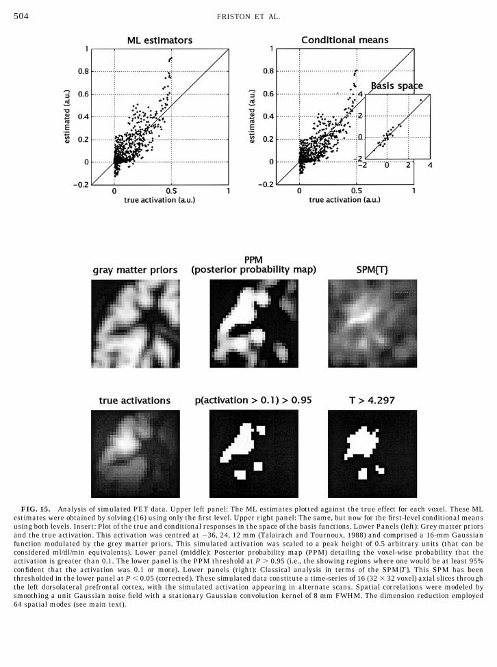
FIG. 15. Analysis of simulated PET data. Upper left panel: The ML estimates plotted against the true effect for each voxel. These MLestimates were obtained by solving (16) using only the first level. Upper right panel: The same, but now for the first-level conditional meansusing both levels. Insert: Plot of the true and conditional responses in the space of the basis functions. Lower Panels (left): Grey matter priorsand the true activation. This activation was centred at �36, 24, 12 mm (Talairach and Tournoux, 1988) and comprised a 16-mm Gaussianfunction modulated by the grey matter priors. This simulated activation was scaled to a peak height of 0.5 arbitrary units (that can beconsidered ml/dl/min equivalents). Lower panel (middle): Posterior probability map (PPM) detailing the voxel-wise probability that theactivation is greater than 0.1. The lower panel is the PPM threshold at P 0.95 (i.e., the showing regions where one would be at least 95%confident that the activation was 0.1 or more). Lower panels (right): Classical analysis in terms of the SPM{T}. This SPM has beenthresholded in the lower panel at P � 0.05 (corrected). These simulated data constitute a time-series of 16 (32 � 32 voxel) axial slices throughthe left dorsolateral prefrontal cortex, with the simulated activation appearing in alternate scans. Spatial correlations were modeled bysmoothing a unit Gaussian noise field with a stationary Gaussian convolution kernel of 8 mm FWHM. The dimension reduction employed64 spatial modes (see main text).

504 FRISTON ET AL.

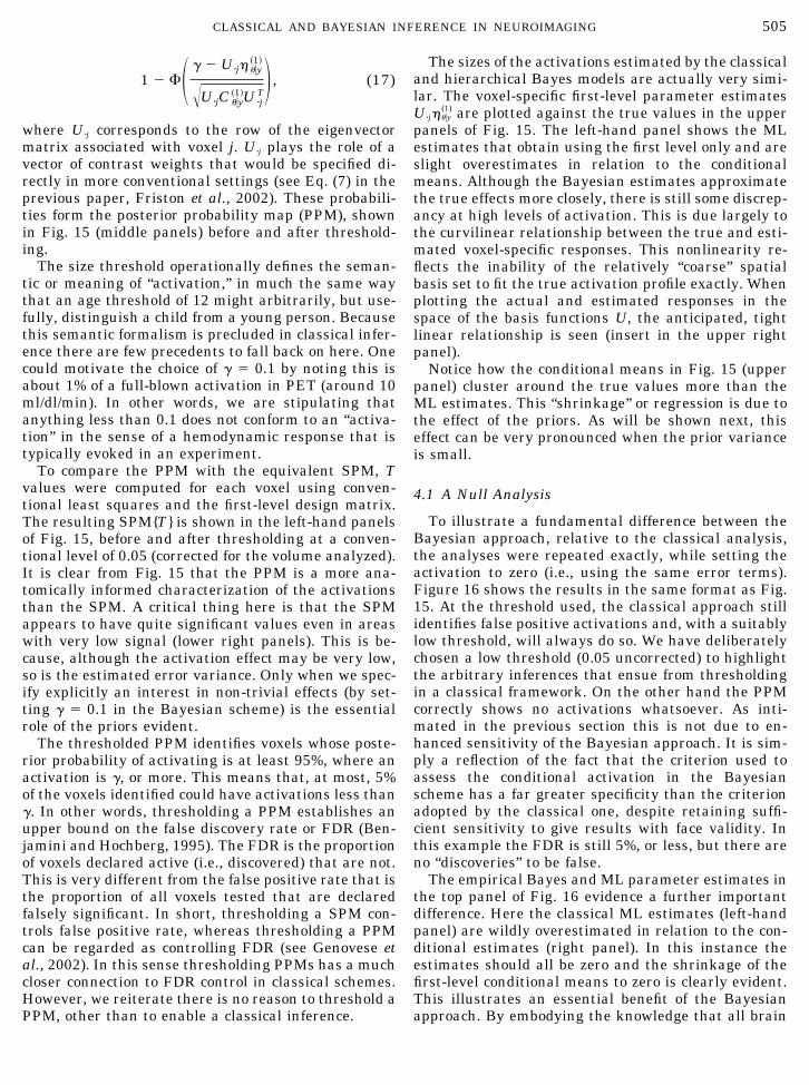
1 � U �j� ��y�1�

�U �jC ��y�1�U �j

T� , (17)

where U �j corresponds to the row of the eigenvectormatrix associated with voxel j. U �j plays the role of avector of contrast weights that would be specified di-rectly in more conventional settings (see Eq. (7) in theprevious paper, Friston et al., 2002). These probabili-ties form the posterior probability map (PPM), shownin Fig. 15 (middle panels) before and after threshold-ing.

The size threshold operationally defines the seman-tic or meaning of “activation,” in much the same waythat an age threshold of 12 might arbitrarily, but use-fully, distinguish a child from a young person. Becausethis semantic formalism is precluded in classical infer-ence there are few precedents to fall back on here. Onecould motivate the choice of � 0.1 by noting this isabout 1% of a full-blown activation in PET (around 10ml/dl/min). In other words, we are stipulating thatanything less than 0.1 does not conform to an “activa-tion” in the sense of a hemodynamic response that istypically evoked in an experiment.

To compare the PPM with the equivalent SPM, Tvalues were computed for each voxel using conven-tional least squares and the first-level design matrix.The resulting SPM{T} is shown in the left-hand panelsof Fig. 15, before and after thresholding at a conven-tional level of 0.05 (corrected for the volume analyzed).It is clear from Fig. 15 that the PPM is a more ana-tomically informed characterization of the activationsthan the SPM. A critical thing here is that the SPMappears to have quite significant values even in areaswith very low signal (lower right panels). This is be-cause, although the activation effect may be very low,so is the estimated error variance. Only when we spec-ify explicitly an interest in non-trivial effects (by set-ting � 0.1 in the Bayesian scheme) is the essentialrole of the priors evident.

The thresholded PPM identifies voxels whose poste-rior probability of activating is at least 95%, where anactivation is , or more. This means that, at most, 5%of the voxels identified could have activations less than. In other words, thresholding a PPM establishes anupper bound on the false discovery rate or FDR (Ben-jamini and Hochberg, 1995). The FDR is the proportionof voxels declared active (i.e., discovered) that are not.This is very different from the false positive rate that isthe proportion of all voxels tested that are declaredfalsely significant. In short, thresholding a SPM con-trols false positive rate, whereas thresholding a PPMcan be regarded as controlling FDR (see Genovese etal., 2002). In this sense thresholding PPMs has a muchcloser connection to FDR control in classical schemes.However, we reiterate there is no reason to threshold aPPM, other than to enable a classical inference.

The sizes of the activations estimated by the classicaland hierarchical Bayes models are actually very simi-lar. The voxel-specific first-level parameter estimatesU �j��y

(1) are plotted against the true values in the upperpanels of Fig. 15. The left-hand panel shows the MLestimates that obtain using the first level only and areslight overestimates in relation to the conditionalmeans. Although the Bayesian estimates approximatethe true effects more closely, there is still some discrep-ancy at high levels of activation. This is due largely tothe curvilinear relationship between the true and esti-mated voxel-specific responses. This nonlinearity re-flects the inability of the relatively “coarse” spatialbasis set to fit the true activation profile exactly. Whenplotting the actual and estimated responses in thespace of the basis functions U, the anticipated, tightlinear relationship is seen (insert in the upper rightpanel).

Notice how the conditional means in Fig. 15 (upperpanel) cluster around the true values more than theML estimates. This “shrinkage” or regression is due tothe effect of the priors. As will be shown next, thiseffect can be very pronounced when the prior varianceis small.

4.1 A Null Analysis

To illustrate a fundamental difference between theBayesian approach, relative to the classical analysis,the analyses were repeated exactly, while setting theactivation to zero (i.e., using the same error terms).Figure 16 shows the results in the same format as Fig.15. At the threshold used, the classical approach stillidentifies false positive activations and, with a suitablylow threshold, will always do so. We have deliberatelychosen a low threshold (0.05 uncorrected) to highlightthe arbitrary inferences that ensue from thresholdingin a classical framework. On the other hand the PPMcorrectly shows no activations whatsoever. As inti-mated in the previous section this is not due to en-hanced sensitivity of the Bayesian approach. It is sim-ply a reflection of the fact that the criterion used toassess the conditional activation in the Bayesianscheme has a far greater specificity than the criterionadopted by the classical one, despite retaining suffi-cient sensitivity to give results with face validity. Inthis example the FDR is still 5%, or less, but there areno “discoveries” to be false.

The empirical Bayes and ML parameter estimates inthe top panel of Fig. 16 evidence a further importantdifference. Here the classical ML estimates (left-handpanel) are wildly overestimated in relation to the con-ditional estimates (right panel). In this instance theestimates should all be zero and the shrinkage of thefirst-level conditional means to zero is clearly evident.This illustrates an essential benefit of the Bayesianapproach. By embodying the knowledge that all brain


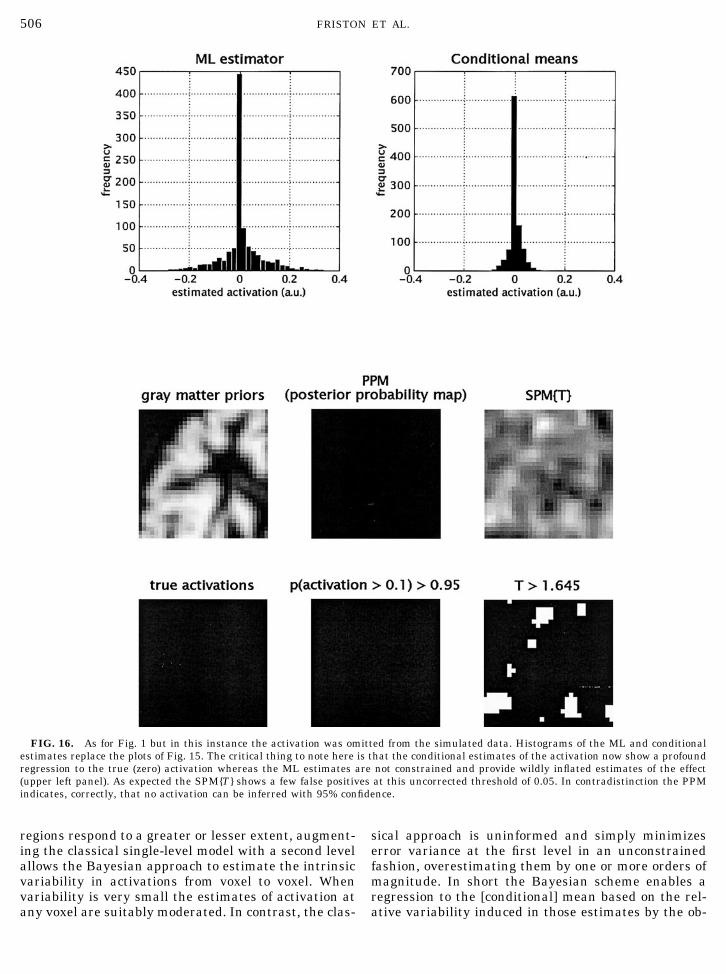
regions respond to a greater or lesser extent, augment-ing the classical single-level model with a second levelallows the Bayesian approach to estimate the intrinsicvariability in activations from voxel to voxel. Whenvariability is very small the estimates of activation atany voxel are suitably moderated. In contrast, the clas-

sical approach is uninformed and simply minimizeserror variance at the first level in an unconstrainedfashion, overestimating them by one or more orders ofmagnitude. In short the Bayesian scheme enables aregression to the [conditional] mean based on the rel-ative variability induced in those estimates by the ob-

FIG. 16. As for Fig. 1 but in this instance the activation was omitted from the simulated data. Histograms of the ML and conditionalestimates replace the plots of Fig. 15. The critical thing to note here is that the conditional estimates of the activation now show a profoundregression to the true (zero) activation whereas the ML estimates are not constrained and provide wildly inflated estimates of the effect(upper left panel). As expected the SPM{T} shows a few false positives at this uncorrected threshold of 0.05. In contradistinction the PPMindicates, correctly, that no activation can be inferred with 95% confidence.

506 FRISTON ET AL.

servation error and the intrinsic variability over vox-els. This is the strength of Bayesian estimators.

5. SPATIOTEMPORAL MODELS:AN EMPIRICAL EXAMPLE

5.1 Analysis of Real Data

In this section we apply the same model to PET datato demonstrate the role of spatial priors in an empiricalsetting. These data are described in the legend to Fig.17. Briefly they came from 5 subjects each scanned 12times while performing a verbal fluency task (ortho-graphic word generation) alternating with a wordshadowing (word repetition) baseline. The modeladopted was exactly the same as above (i.e., Eq. (16))with one exception. In the simulations the error vari-ance was the same for all voxels. However, in the realbrain, error variance may change from brain structureto brain structure. This is accommodated easily byexpanding the constraints on the error covariances tocover the nonstationariness of error variance antici-pated. Here we adopt a very simple model and assumethat error variance has two components, one that isstationary (as used above) and one that conforms to thesame spatial profile as the hemodynamic signal itself,where, prior to reduction

Q 1�1� � PP T

(18)Q 2

�1� � P�Q 1�2� � It�P T.

As in the simulations the intrinsic correlation matrix Dwas Gaussian with 4 mm FWHM. The point spreadfunction was Gaussian with 16 mm FWHM, corre-sponding to the smoothing kernel applied to the dataafter spatial normalization. The motivation forsmoothing the data, and then incorporating thesmoothing kernel in the estimation model, is that onecan reduce variations in spatial correlations from scanto scan and subject to subject. Furthermore, this allowsone to accommodate variation in gyral and functionalanatomy among subjects that is smaller than thesmoothing kernel. By smoothing the data and thenapplying the same anatomical constraints we effec-tively estimate what would have been observed if everysubject had exactly the same neuroanatomy, namelythat of the standard space used in anatomical normal-ization and to derive the priors. Subject-specific effects,linear time effects, global effects, and the constantterm were all treated as nuisance variables and wereremoved from the data (and design matrix) prior toestimation.11 As above, each partition of the block di-

agonal first level design matrix was a single column ofalternating �1 s and �1 s depending on whether thescan was an activation scan or baseline. The adjusteddata were entered into the EM algorithm as above.

The results of the analysis are presented in Fig. 17using a similar format to Figs. 15 and 16. In thisinstance we show the ML estimators (upper panel) thatobtain from a voxel by voxel estimation, i.e., withoutusing spatial basis functions or incorporating the pointspread function into the estimation model. We omittedthese components to show (i) the impoverished spatialresolution (lower panels) and (ii) partial volume effectthat ensues (upper panel). The PPM and SPM arepleasingly congruent particularly in light of the realis-tic threshold used for the SPM{T} (0.05 corrected).However, the enhanced spatial information availablein the PPM, relative to the SPM is immediately obvi-ous. The slice shown is at 12 mm above the ACPC line.The regions showing an activation of 0.1 ml/dl/min(Equivalents), or more, comprise Broca’s area (BA 44)and contiguous premotor cortex (BA 6), an activationdeep in the anterior frontal operculum and a subcorti-cal activation centred on the mediodorsal nucleus ofthe thalamus. This anatomical precision could not besupported using the conventional SPM (right handpanels in Fig. 17). Equally interesting are the condi-tional means and ML estimates in the upper panel.The critical thing to note here is that, due to smoothingor partial volume effects, the ML estimates (dots) aretoo small. Because the conditional means (line) areinformed about the spatial configuration of sources,subtending signals observed after convolution, they areapproximately twice as large. This suggests (as wealready knew) that conventional analyses can substan-tially underestimate true effects, especially when theyare focal.

5.2 Summary

In this section we have illustrated how Bayesianestimates can supervene over classical ML estimatesby harnessing constraints at higher levels. We haveused spatial constraints in this example and intro-duced spatiotemporal models to this end. The keypoints include:

● The notion that observations over voxels representrepeated measures of the same neuronal response.This motivates a two-level hierarchical observationmodel and enables Bayesian inference at the first[voxel] level. The first-level conditional estimates aregenerally better than conventional ML estimates be-

11 This is not necessary because we could have simply includedthese effects in the first-level design. However, given the computa-tional load of spatiotemporal models, it is sometimes easier to treat

nuisance variables and confounds as fixed effects and remove thembefore applying the EM algorithm. Note that when this is done thecovariance constraints are assumed to hold for the adjusted data, asopposed to the original data.


FIG. 17. Analysis of real PET data. The layout of this figure corresponds to Figs. 15 and 16 but in this instance the true activation isunknown (the lower right panel simply shows the structural image on which the priors were based). These data came from a PET study ofpaced FAS orthographic verbal fluency in which five subjects were asked to produce words beginning with a heard letter (word generation)or simply repeat the letter (word shadowing). These two conditions alternated for 12 scans. In this analysis we treated all 60 scans as if theycame from the same subject because we wanted to illustrate second-level constraints in terms of spatial realizations over voxels. The datawere smoothed with a 16-mm FWHM Gaussian kernel, which ameliorates differences in functional anatomy among subjects. The resultsshown are for a 32 � 64 (2 � 2 � 2 mm) voxel slice through the left hemisphere at z � 12 mm. The SPM{T} is based on a conventionalvoxel-wise approach that benefits from neither the dimension reduction (hard constraints afforded by the grey matter priors) or the Bayesianestimation (soft constraints). Consequently the classical analysis has markedly poorer anatomical resolution and is subject to partial volume

508 FRISTON ET AL.

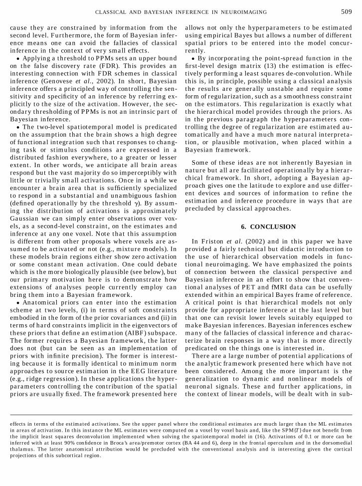
cause they are constrained by information from thesecond level. Furthermore, the form of Bayesian infer-ence means one can avoid the fallacies of classicalinference in the context of very small effects.

● Applying a threshold to PPMs sets an upper boundon the false discovery rate (FDR). This provides aninteresting connection with FDR schemes in classicalinference (Genovese et al., 2002). In short, Bayesianinference offers a principled way of controlling the sen-sitivity and specificity of an inference by referring ex-plicitly to the size of the activation. However, the sec-ondary thresholding of PPMs is not an intrinsic part ofBayesian inference.

● The two-level spatiotemporal model is predicatedon the assumption that the brain shows a high degreeof functional integration such that responses to chang-ing task or stimulus conditions are expressed in adistributed fashion everywhere, to a greater or lesserextent. In other words, we anticipate all brain areasrespond but the vast majority do so imperceptibly withlittle or trivially small activations. Once in a while weencounter a brain area that is sufficiently specializedto respond in a substantial and unambiguous fashion(defined operationally by the threshold ). By assum-ing the distribution of activations is approximatelyGaussian we can simply enter observations over vox-els, as a second-level constraint, on the estimates andinference at any one voxel. Note that this assumptionis different from other proposals where voxels are as-sumed to be activated or not (e.g., mixture models). Inthese models brain regions either show zero activationor some constant mean activation. One could debatewhich is the more biologically plausible (see below), butour primary motivation here is to demonstrate howextensions of analyses people currently employ canbring them into a Bayesian framework.

● Anatomical priors can enter into the estimationscheme at two levels, (i) in terms of soft constraintsembodied in the form of the prior covariances and (ii) interms of hard constraints implicit in the eigenvectors ofthese priors that define an estimation (AIBF) subspace.The former requires a Bayesian framework, the latterdoes not (but can be seen as an implementation ofpriors with infinite precision). The former is interest-ing because it is formally identical to minimum normapproaches to source estimation in the EEG literature(e.g., ridge regression). In these applications the hyper-parameters controlling the contribution of the spatialpriors are usually fixed. The framework presented here

allows not only the hyperparameters to be estimatedusing empirical Bayes but allows a number of differentspatial priors to be entered into the model concur-rently.

● By incorporating the point-spread function in thefirst-level design matrix (13) the estimation is effec-tively performing a least squares de-convolution. Whilethis is, in principle, possible using a classical analysisthe results are generally unstable and require someform of regularization, such as a smoothness constrainton the estimators. This regularization is exactly whatthe hierarchical model provides through the priors. Asin the previous paragraph the hyperparameters con-trolling the degree of regularization are estimated au-tomatically and have a much more natural interpreta-tion, or plausible motivation, when placed within aBayesian framework.

Some of these ideas are not inherently Bayesian innature but all are facilitated operationally by a hierar-chical framework. In short, adopting a Bayesian ap-proach gives one the latitude to explore and use differ-ent devices and sources of information to refine theestimation and inference procedure in ways that areprecluded by classical approaches.

6. CONCLUSION

In Friston et al. (2002) and in this paper we haveprovided a fairly technical but didactic introduction tothe use of hierarchical observation models in func-tional neuroimaging. We have emphasized the pointsof connection between the classical perspective andBayesian inference in an effort to show that conven-tional analyses of PET and fMRI data can be usefullyextended within an empirical Bayes frame of reference.A critical point is that hierarchical models not onlyprovide for appropriate inference at the last level butthat one can revisit lower levels suitably equipped tomake Bayesian inferences. Bayesian inferences eschewmany of the fallacies of classical inference and charac-terize brain responses in a way that is more directlypredicated on the things one is interested in.

There are a large number of potential applications ofthe analytic framework presented here which have notbeen considered. Among the more important is thegeneralization to dynamic and nonlinear models ofneuronal signals. These and further applications, inthe context of linear models, will be dealt with in sub-

effects in terms of the estimated activations. See the upper panel where the conditional estimates are much larger than the ML estimatesin areas of activation. In this instance the ML estimates were computed on a voxel by voxel basis and, like the SPM{T} due not benefit fromthe implicit least squares deconvolution implemented when solving the spatiotemporal model in (16). Activations of 0.1 or more can beinferred with at least 90% confidence in Broca’s area/premotor cortex (BA 44 and 6), deep in the frontal operculum and in the dorsomedialthalamus. The latter anatomical attribution would be precluded with the conventional analysis and is interesting given the corticalprojections of this subcortical region.


sequent papers (e.g., Friston, 2002). The examples inthis paper are used to illustrate ideas and serve as“proof of concept.” In particular, conclusions regardingsensitivity and specificity pertain only to the specificdata considered.

The drawbacks of empirical Bayes estimation andinference procedures are theoretical and practical.Practical difficulties are related simply to computa-tional load and time of processing (see software imple-mentation note below). The theoretical difficulties in-clude the overconfidence problem.

6.1 The Overconfidence Problem

In PEB methods the hyperparameters pertaining tothe covariance components are estimated by maximumlikelihood and are then used to compute the posteriormeans and covariance of the parameters. From a fullyBayesian perspective the PEB approach effectivelysubstitutes the conditional posterior density, p(��y, �)with � � �̂ for the correct posterior density given by

p��y� � � p��y, ��p��y�d�. (19)

Thus the PEB approximation fails to take account ofthe uncertainty about the hyperparameters that entersthrough p(��y). It is well known that the posterior meanconditional on the ReML estimate �̂ is approximatelyequal to the true posterior mean. However, the corre-sponding conditional posterior covariance is too small(Kass and Steffrey, 1989). This results in over confi-dence when making inferences using PEB methodol-ogy. In other words, although the empirical posteriorresponse estimates are good approximations, infer-ences about them may be slightly capricious. Kass andSteffrey (1989) provide a solution to this problem forconditionally independent hierarchical models, where

Cov��y� � E�Cov��y, �̂ � Cov�E��y, �̂

C��y � ��y

�Cov��y

��yT

�,

(20)

where the expectation and covariance are with respectto the posterior distribution of �. This provides for afirst order approximation to the second term in the firstline of (20), using the delta method (i.e., a first-orderTaylor expansion) and the posterior covariance of thehyperparameters (the second line of 20). This is, inprinciple, feasible but requires the specification of botha likelihood function, of its sufficient statistics, and aprior density function for the hyperparameters. Effec-tively this means replacing the ML estimate of thehyperparameters with its conditional mean and aug-

menting the conditional posterior covariance with thesecond term above. The choice of these likelihood func-tions and priors can sometimes be quite arbitrary andmotivated by mathematical convenience (e.g., conju-gate priors). While providing the basis for interestingextensions of PEB for neuroimaging we have chosen toavoid this issue by treating the hyperparameters asfixed effects and eschewing the need to specify a like-lihood. Consequently we adhere to an empirical frame-work, which assumes that the second term in (20) issufficiently small to be ignored. An interesting possi-bility is to use a PEB estimator of the hyperparametersthemselves. This would lead to a truly recursive algo-rithm but this is beyond the scope of these papers.

6.2 Priors

A general issue in Bayesian models of spatiotempo-ral responses is the face validity of the model adopted.For example, in this paper we have assumed that theprior distribution of responses, over voxels, is Gauss-ian. The ensuing hierarchical model uses the between-voxel variability as a prior variance on the response ofany single voxel. Other models could be used, for ex-ample mixture models (Everitt and Bullmore, 1999).Mixture models assume that data are generated by asmall number of “causes,” each parameterized by adifferent activation level. Inference can be based on theposterior probability that a voxel belongs a particularcomponent of the mixture, where each component ischaracterized by its estimated activation. In Penny andFriston (2002) we show how mixtures of general linearmodels can be estimated using EM. Whether a mixturemodel is more or less appropriate than the hierarchicalmodel presented in this paper is an outstanding ques-tion. Indeed knowing which model is best would im-plicitly resolve some fundamental questions aboutfunctional brain architectures. Mixture models can beseen as taking functional segregation to its extreme.Functional segregation posits that a particular cogni-tive or sensorimotor function is served by functionalitythat is anatomical segregated in one part of the brain.This implies that the segregated area will respond toexperimental challenge and that remaining areas willnot. The empirical Bayes model considered above al-lows for functional specialization assuming thatevoked responses are distributed but are expressedmuch more in specialized areas. This is consistent withperspectives offered by cognitive neuroscience (e.g.,parallel distributed processing). Conversely, the hier-archical model represents an extreme of functional in-tegration, in which regional specialization is onlyquantitative. A simple refinement of the model in thispaper could involve super-Gaussian priors that modela small number of highly responsive voxels and a largenumber of relatively unresponsive voxels. By hyperpa-rameterizing non-Gaussian priors of this sort the de-

510 FRISTON ET AL.

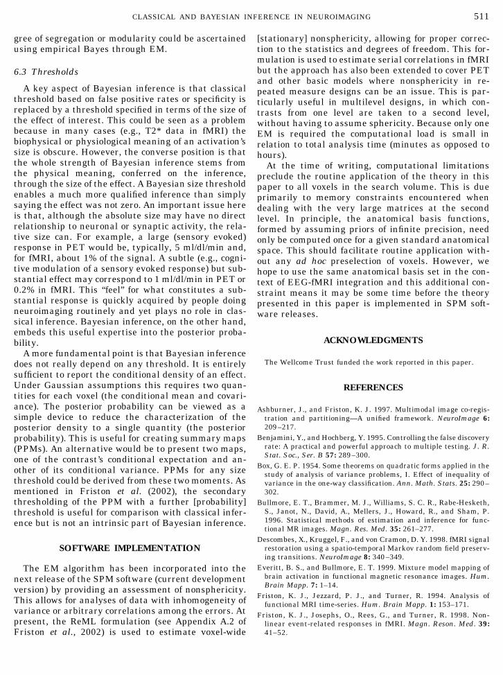
gree of segregation or modularity could be ascertainedusing empirical Bayes through EM.

6.3 Thresholds

A key aspect of Bayesian inference is that classicalthreshold based on false positive rates or specificity isreplaced by a threshold specified in terms of the size ofthe effect of interest. This could be seen as a problembecause in many cases (e.g., T2* data in fMRI) thebiophysical or physiological meaning of an activation’ssize is obscure. However, the converse position is thatthe whole strength of Bayesian inference stems fromthe physical meaning, conferred on the inference,through the size of the effect. A Bayesian size thresholdenables a much more qualified inference than simplysaying the effect was not zero. An important issue hereis that, although the absolute size may have no directrelationship to neuronal or synaptic activity, the rela-tive size can. For example, a large (sensory evoked)response in PET would be, typically, 5 ml/dl/min and,for fMRI, about 1% of the signal. A subtle (e.g., cogni-tive modulation of a sensory evoked response) but sub-stantial effect may correspond to 1 ml/dl/min in PET or0.2% in fMRI. This “feel” for what constitutes a sub-stantial response is quickly acquired by people doingneuroimaging routinely and yet plays no role in clas-sical inference. Bayesian inference, on the other hand,embeds this useful expertise into the posterior proba-bility.

A more fundamental point is that Bayesian inferencedoes not really depend on any threshold. It is entirelysufficient to report the conditional density of an effect.Under Gaussian assumptions this requires two quan-tities for each voxel (the conditional mean and covari-ance). The posterior probability can be viewed as asimple device to reduce the characterization of theposterior density to a single quantity (the posteriorprobability). This is useful for creating summary maps(PPMs). An alternative would be to present two maps,one of the contrast’s conditional expectation and an-other of its conditional variance. PPMs for any sizethreshold could be derived from these two moments. Asmentioned in Friston et al. (2002), the secondarythresholding of the PPM with a further [probability]threshold is useful for comparison with classical infer-ence but is not an intrinsic part of Bayesian inference.

SOFTWARE IMPLEMENTATION

The EM algorithm has been incorporated into thenext release of the SPM software (current developmentversion) by providing an assessment of nonsphericity.This allows for analyses of data with inhomogeneity ofvariance or arbitrary correlations among the errors. Atpresent, the ReML formulation (see Appendix A.2 ofFriston et al., 2002) is used to estimate voxel-wide

[stationary] nonsphericity, allowing for proper correc-tion to the statistics and degrees of freedom. This for-mulation is used to estimate serial correlations in fMRIbut the approach has also been extended to cover PETand other basic models where nonsphericity in re-peated measure designs can be an issue. This is par-ticularly useful in multilevel designs, in which con-trasts from one level are taken to a second level,without having to assume sphericity. Because only oneEM is required the computational load is small inrelation to total analysis time (minutes as opposed tohours).

At the time of writing, computational limitationspreclude the routine application of the theory in thispaper to all voxels in the search volume. This is dueprimarily to memory constraints encountered whendealing with the very large matrices at the secondlevel. In principle, the anatomical basis functions,formed by assuming priors of infinite precision, needonly be computed once for a given standard anatomicalspace. This should facilitate routine application with-out any ad hoc preselection of voxels. However, wehope to use the same anatomical basis set in the con-text of EEG-fMRI integration and this additional con-straint means it may be some time before the theorypresented in this paper is implemented in SPM soft-ware releases.

ACKNOWLEDGMENTS

The Wellcome Trust funded the work reported in this paper.

REFERENCES

Ashburner, J., and Friston, K. J. 1997. Multimodal image co-regis-tration and partitioning—A unified framework. NeuroImage 6:209–217.

Benjamini, Y., and Hochberg, Y. 1995. Controlling the false discoveryrate: A practical and powerful approach to multiple testing. J. R.Stat. Soc., Ser. B 57: 289–300.

Box, G. E. P. 1954. Some theorems on quadratic forms applied in thestudy of analysis of variance problems, I. Effect of inequality ofvariance in the one-way classification. Ann. Math. Stats. 25: 290–302.

Bullmore, E. T., Brammer, M. J., Williams, S. C. R., Rabe-Hesketh,S., Janot, N., David, A., Mellers, J., Howard, R., and Sham, P.1996. Statistical methods of estimation and inference for func-tional MR images. Magn. Res. Med. 35: 261–277.

Descombes, X., Kruggel, F., and von Cramon, D. Y. 1998. fMRI signalrestoration using a spatio-temporal Markov random field preserv-ing transitions. NeuroImage 8: 340–349.

Everitt, B. S., and Bullmore, E. T. 1999. Mixture model mapping ofbrain activation in functional magnetic resonance images. Hum.Brain Mapp. 7: 1–14.

Friston, K. J., Jezzard, P. J., and Turner, R. 1994. Analysis offunctional MRI time-series. Hum. Brain Mapp. 1: 153–171.

Friston, K. J., Josephs, O., Rees, G., and Turner, R. 1998. Non-linear event-related responses in fMRI. Magn. Reson. Med. 39:41–52.


Friston, K. J., Josephs, O., Zarahn, E., Holmes, A. P., Rouquette, S.,and Poline, J.-B. 2000. To smooth or not to smooth? Bias andefficiency in fMRI time-series analysis. NeuroImage 12: 196–208.

Friston, K. J., Penny, W., Phillips, C., Kiebel, S., Hinton, G., andAshburner, J. 2002. Classical and Bayesian inference in neuro-imaging: Theory. NeuroImage 16: 465–483.

Friston, K. J. 2002. Bayesian estimation of dynamical systems: Anapplication to fMRI. NeuroImage 16: 513–530.

Genovese, C. R., Lazar, N. A., and Nichols, T. E. 2002. Thresholdingof statistical maps in functional neuroimaging using the falsediscovery rate. NeuroImage, submitted.

Geisser, S., and Greenhouse, S. W. 1958. An extension of Box’sresults on the use of the F distribution in multivariate analysis.Ann. Math. Stats. 29: 885–891.

Hartvig, N. V., and Jensen, J. L. 2000. Spatial mixture modelling offMRI data. Hum. Brain Mapp., in press.

Henson, R. N. A., Rugg, M. D., Shallice, T., and Dolan, R. J. 2000.Confidence in recognition memory for words: Dissociating rightprefrontal roles in episodic retrieval. J. Cogn. Neurosci., in press.

Højen-Sørensen, P., Hansen, L. K., and Rasmussen, C. E. 2000.Bayesian modelling of fMRI time-series. In Advances in NeuralInformation Processing Systems (S. A. Solla, T. K. Leen, and K. R.Muller, Eds.), Vol. 12, pp. 754–760. MIT Press.

Kass, R. E., and Steffey, D. 1989. Approximate Bayesian inference inconditionally independent hierarchical models (parametric empir-ical Bayes models). J. Am. Stat. Assoc. 407: 717–726.

Kiebel, S., Goebel, R., and Friston, K. J. 2000. Anatomically informedbasis functions. NeuroImage 11: 656–667.

Penny, W., and Friston, K. J. 2002. Mixtures of general linear modelsfor neuroimaging. Submitted.

Phillips, C., Rugg, M. D., and Friston, K. J. 1999. Informed spatial basisfunctions in minimum norm solutions for the electromagnetic sourcelocalisation problem. Biomedizinische technik. 2: 87–90.

Purdon, P. L., and Weisskoff, R. 1998. Effect of temporal autocorre-lations due to physiological noise stimulus paradigm on voxel-levelfalse positive rates in fMRI. Hum. Brain Mapp. 6: 239–249.

Satterthwaite, E. F. 1941. Synthesis of variance. Psychometrika 6:309–316.

Talairach, J., and Tournoux, P. 1988. A Co-planar Stereotaxic Atlasof a Human Brain. Thieme, Stuttgart.

Worsley, K. J., and Friston, K. J. 1995. Analysis of fMRI time-seriesrevisited—Again. NeuroImage 2: 173–181.

Worsley, K. J., Liao, C., Aston, J., Petre, V., Duncan, G. H., andEvans, A. C. 2002. A general statistical analysis for fMRI data.NeuroImage 15: 1–15.

512 FRISTON ET AL.

Documents

Classical and Bayesian Inference in Neuroimaging: Applications