Classification and Prediction. What is classification? What is prediction? Issues regarding classification and prediction Classification by decision

Classification and Prediction


What is classification? What is prediction? Issues regarding classification and prediction Classification by decision tree induction Bayesian Classification Classification based on concepts from

association rule mining Other Classification Methods Prediction Classification accuracy Summary

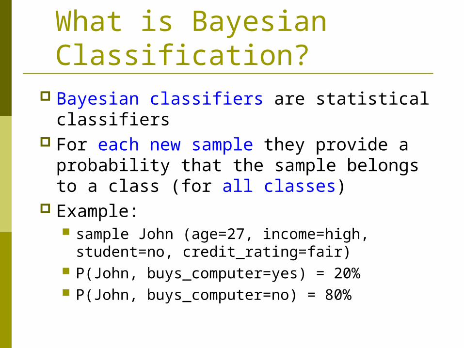
What is Bayesian Classification?

Bayesian classifiers are statistical classifiers

For each new sample they provide a probability that the sample belongs to a class (for all classes)

Example: sample John (age=27, income=high,

student=no, credit_rating=fair) P(John, buys_computer=yes) = 20% P(John, buys_computer=no) = 80%

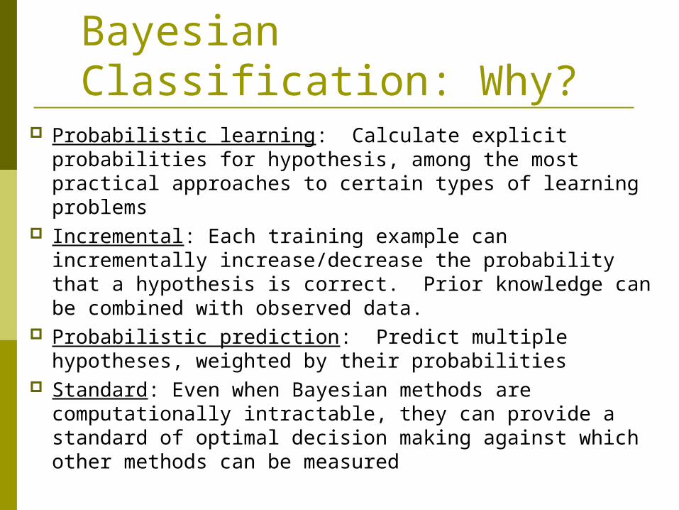
Bayesian Classification: Why?

Probabilistic learning: Calculate explicit probabilities for hypothesis, among the most practical approaches to certain types of learning problems

Incremental: Each training example can incrementally increase/decrease the probability that a hypothesis is correct. Prior knowledge can be combined with observed data.

Probabilistic prediction: Predict multiple hypotheses, weighted by their probabilities

Standard: Even when Bayesian methods are computationally intractable, they can provide a standard of optimal decision making against which other methods can be measured

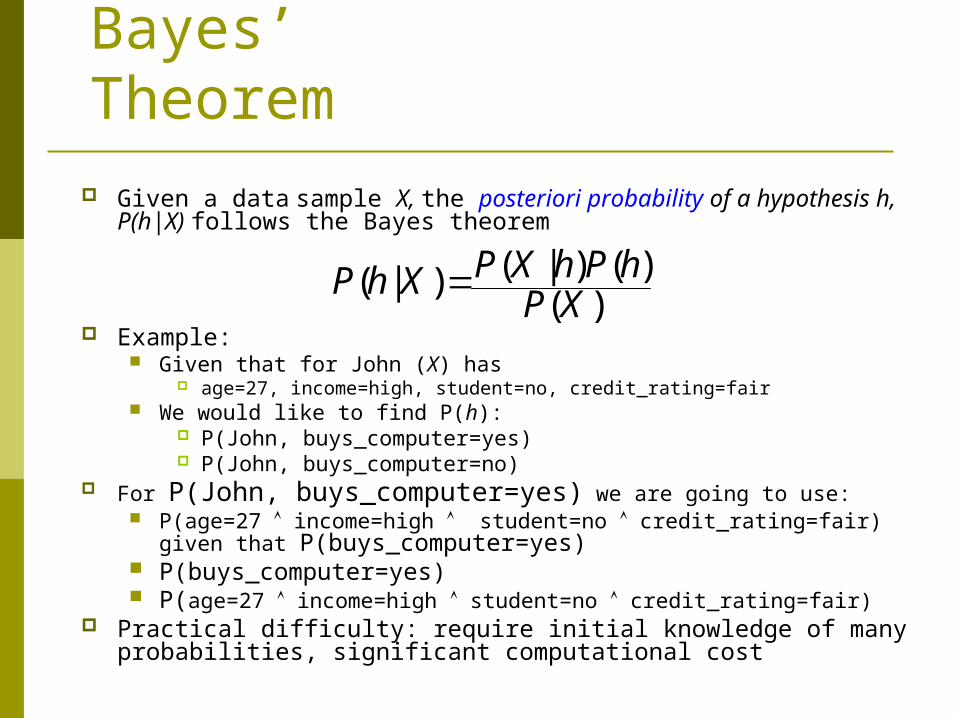
Bayes’ Theorem

Given a data sample X, the posteriori probability of a hypothesis h, P(h|X) follows the Bayes theorem

Example: Given that for John (X) has

age=27, income=high, student=no, credit_rating=fair We would like to find P(h):

P(John, buys_computer=yes) P(John, buys_computer=no)

For P(John, buys_computer=yes) we are going to use: P(age=27 income=high student=no credit_rating=fair) given

that P(buys_computer=yes) P(buys_computer=yes) P(age=27 income=high student=no credit_rating=fair)

Practical difficulty: require initial knowledge of many probabilities, significant computational cost

)()()|()|(

XPhPhXPXhP

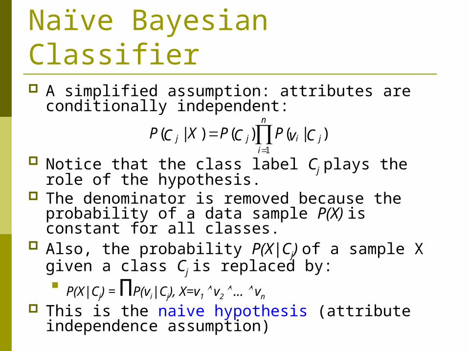
Naïve Bayesian Classifier A simplified assumption: attributes are

conditionally independent:

Notice that the class label Cj plays the role of the hypothesis.

The denominator is removed because the probability of a data sample P(X) is constant for all classes.

Also, the probability P(X|Cj) of a sample X given a class Cj is replaced by: P(X|Cj) = ΠP(vi|Cj), X=v1 v2 ... vn

This is the naive hypothesis (attribute independence assumption)

n

ijijj CvPCPXCP

1

)|()()|(

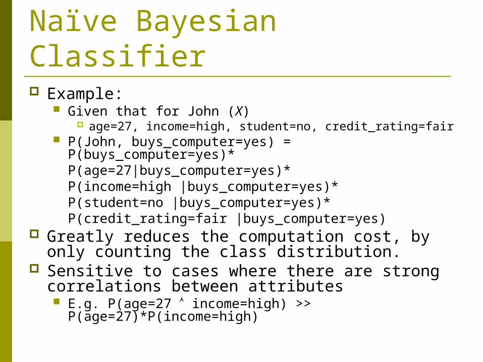
Naïve Bayesian Classifier Example:

Given that for John (X) age=27, income=high, student=no, credit_rating=fair

P(John, buys_computer=yes) = P(buys_computer=yes)*P(age=27|buys_computer=yes)*P(income=high |buys_computer=yes)*P(student=no |buys_computer=yes)*P(credit_rating=fair |buys_computer=yes)

Greatly reduces the computation cost, by only counting the class distribution.

Sensitive to cases where there are strong correlations between attributes E.g. P(age=27 income=high) >>

P(age=27)*P(income=high)

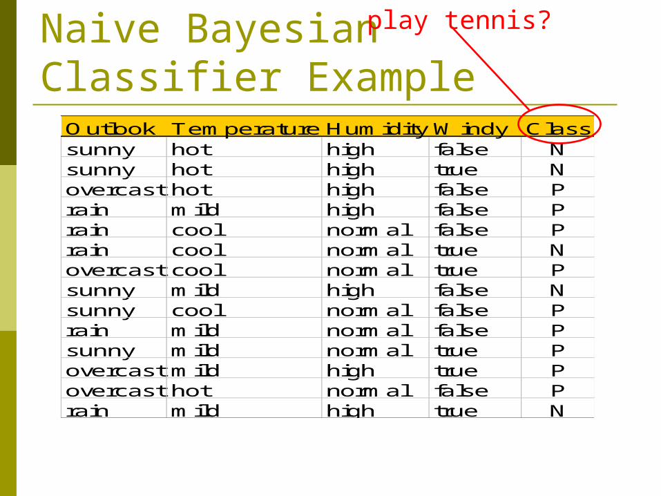
Naive Bayesian Classifier ExampleOutlook Temperature Humidity Windy Classsunny hot high false Nsunny hot high true Novercast hot high false Prain mild high false Prain cool normal false Prain cool normal true Novercast cool normal true Psunny mild high false Nsunny cool normal false Prain mild normal false Psunny mild normal true Povercast mild high true Povercast hot normal false Prain mild high true N

play tennis?

Naive Bayesian Classifier Example

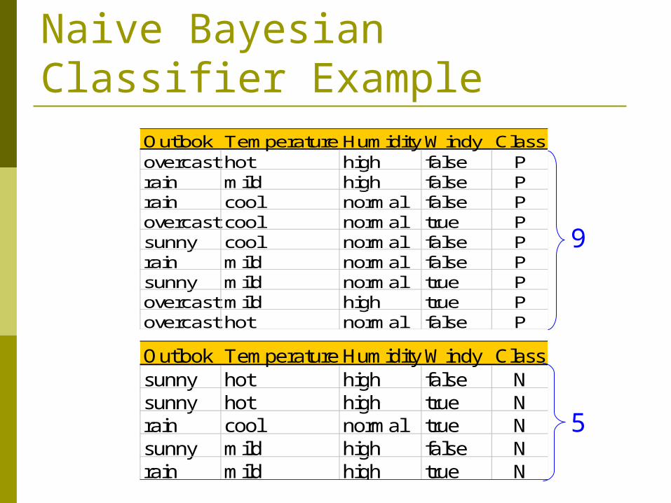
Outlook Temperature HumidityWindy Classsunny hot high false Nsunny hot high true Nrain cool normal true Nsunny mild high false Nrain mild high true N

Outlook Temperature HumidityWindy Classovercast hot high false Prain mild high false Prain cool normal false Povercast cool normal true Psunny cool normal false Prain mild normal false Psunny mild normal true Povercast mild high true Povercast hot normal false P

9

5

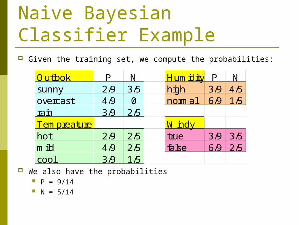
Naive Bayesian Classifier Example Given the training set, we compute the probabilities:

We also have the probabilities P = 9/14 N = 5/14

Outlook P N Humidity P Nsunny 2/9 3/5 high 3/9 4/5overcast 4/9 0 normal 6/9 1/5rain 3/9 2/5Tempreature Windyhot 2/9 2/5 true 3/9 3/5mild 4/9 2/5 false 6/9 2/5cool 3/9 1/5


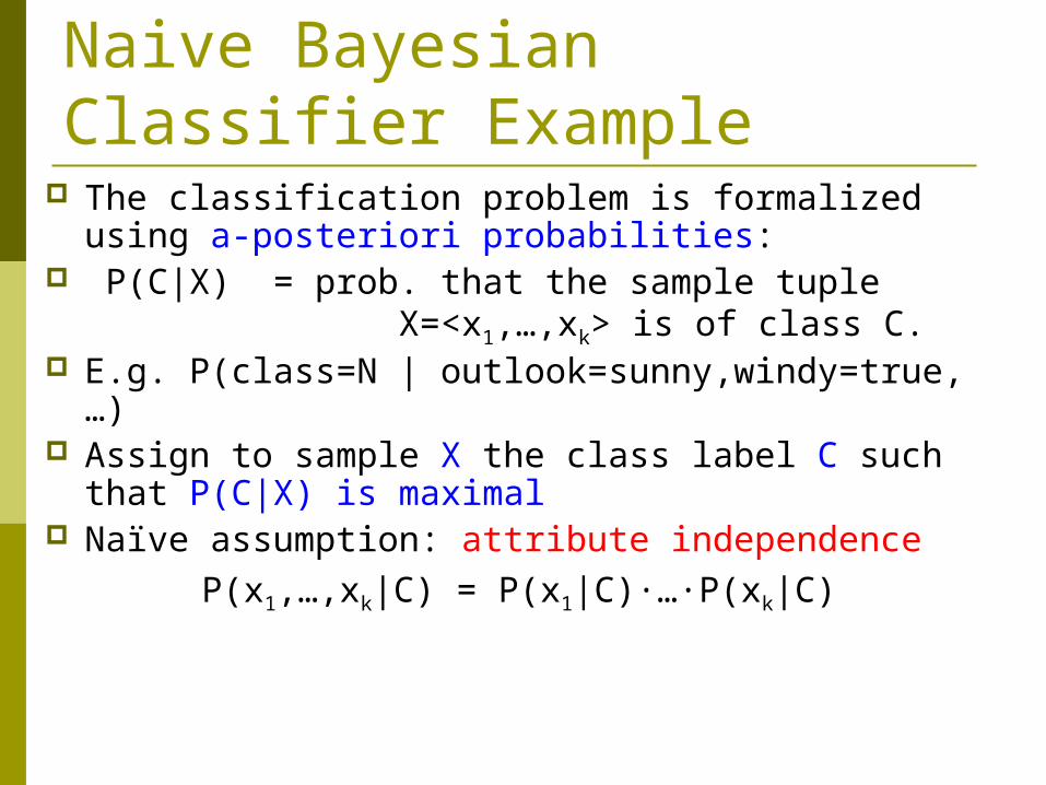
The classification problem is formalized using a-posteriori probabilities:

P(C|X) = prob. that the sample tuple X=<x1,…,xk> is of class C.

E.g. P(class=N | outlook=sunny,windy=true,…) Assign to sample X the class label C such that P(C|

X) is maximal Naïve assumption: attribute independence

P(x1,…,xk|C) = P(x1|C)·…·P(xk|C)

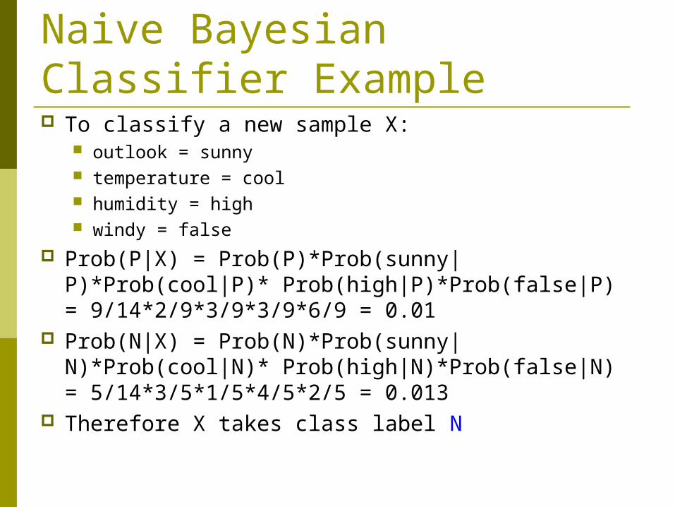
Naive Bayesian Classifier Example To classify a new sample X:

outlook = sunny temperature = cool humidity = high windy = false

Prob(P|X) = Prob(P)*Prob(sunny|P)*Prob(cool|P)* Prob(high|P)*Prob(false|P) = 9/14*2/9*3/9*3/9*6/9 = 0.01

Prob(N|X) = Prob(N)*Prob(sunny|N)*Prob(cool|N)* Prob(high|N)*Prob(false|N) = 5/14*3/5*1/5*4/5*2/5 = 0.013

Therefore X takes class label N

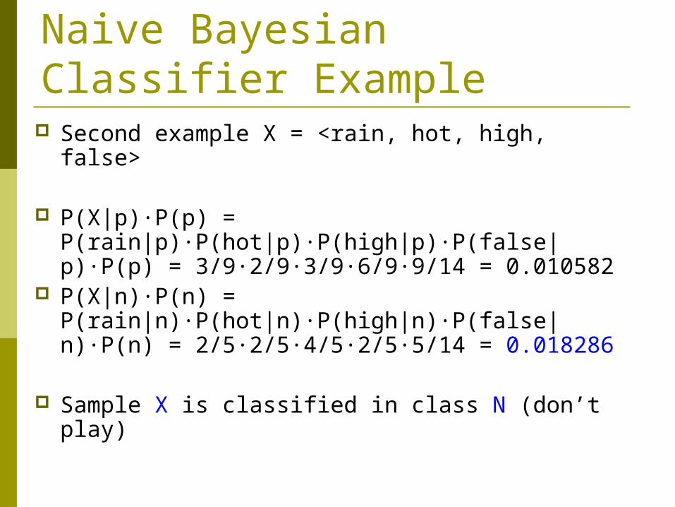
Second example X = <rain, hot, high, false>

P(X|p)·P(p) = P(rain|p)·P(hot|p)·P(high|p)·P(false|p)·P(p) = 3/9·2/9·3/9·6/9·9/14 = 0.010582

P(X|n)·P(n) = P(rain|n)·P(hot|n)·P(high|n)·P(false|n)·P(n) = 2/5·2/5·4/5·2/5·5/14 = 0.018286

Sample X is classified in class N (don’t play)


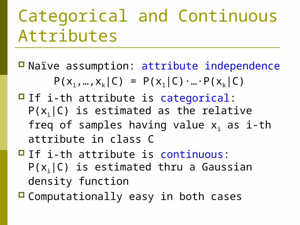
Categorical and Continuous Attributes

Naïve assumption: attribute independenceP(x1,…,xk|C) = P(x1|C)·…·P(xk|C)

If i-th attribute is categorical:P(xi|C) is estimated as the relative freq of samples having value xi as i-th attribute in class C

If i-th attribute is continuous:P(xi|C) is estimated thru a Gaussian density function

Computationally easy in both cases

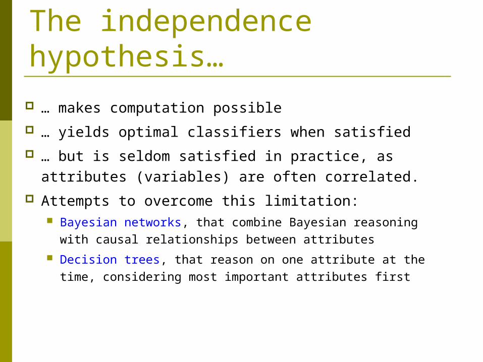
The independence hypothesis…

… makes computation possible

… yields optimal classifiers when satisfied

… but is seldom satisfied in practice, as attributes (variables) are often correlated.

Attempts to overcome this limitation: Bayesian networks, that combine Bayesian reasoning

with causal relationships between attributes

Decision trees, that reason on one attribute at the time, considering most important attributes first

Bayesian Belief Networks (I) A directed acyclic graph which models

dependencies between variables (values) If an arc is drawn from node Y to node Z,

then Z depends on Y Z is a child (descendant) of Y Y is a parent (ancestor) of Z

Each variable is conditionally independent of its nondescendants given its parents

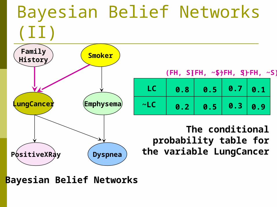
Bayesian Belief Networks (II)

FamilyHistory

LungCancer

PositiveXRay

Smoker

Emphysema

Dyspnea

LC

~LC

(FH, S) (FH, ~S)(~FH, S) (~FH, ~S)

0.8

0.2

0.5

0.5

0.7

0.3

0.1

0.9

Bayesian Belief Networks

The conditional probability table for the variable LungCancer

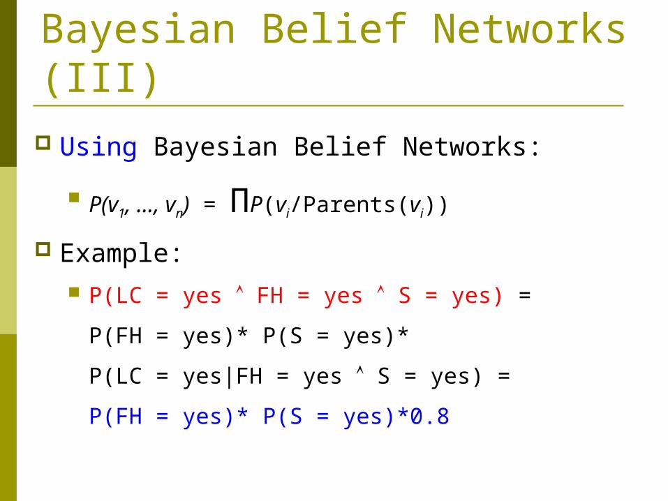
Bayesian Belief Networks (III) Using Bayesian Belief Networks:

P(v1, ..., vn) = ΠP(vi/Parents(vi))

Example: P(LC = yes FH = yes S = yes) =

P(FH = yes)* P(S = yes)*

P(LC = yes|FH = yes S = yes) =

P(FH = yes)* P(S = yes)*0.8

Bayesian Belief Networks (IV) Bayesian belief network allows a subset of the

variables conditionally independent

A graphical model of causal relationships

Several cases of learning Bayesian belief networks Given both network structure and all the variables: easy

Given network structure but only some variables

When the network structure is not known in advance

Classification and Prediction What is classification? What is prediction? Issues regarding classification and prediction Classification by decision tree induction Bayesian Classification Classification based on concepts from


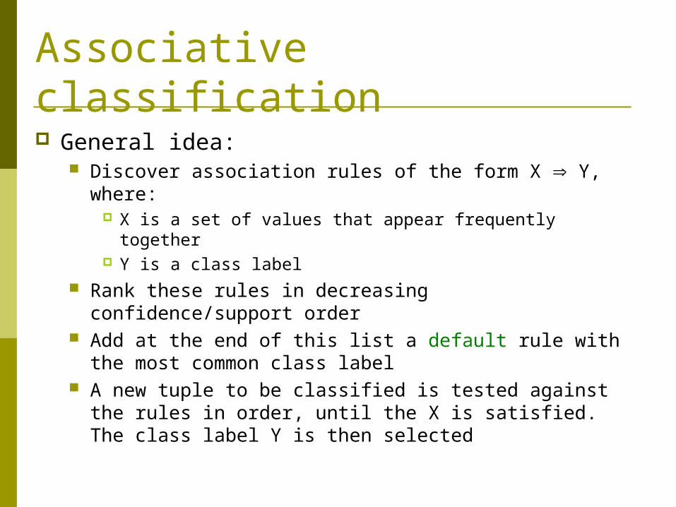
Associative classification General idea:

Discover association rules of the form X Y, where: X is a set of values that appear frequently together Y is a class label

Rank these rules in decreasing confidence/support order Add at the end of this list a default rule with the most

common class label A new tuple to be classified is tested against the rules in

order, until the X is satisfied. The class label Y is then selected

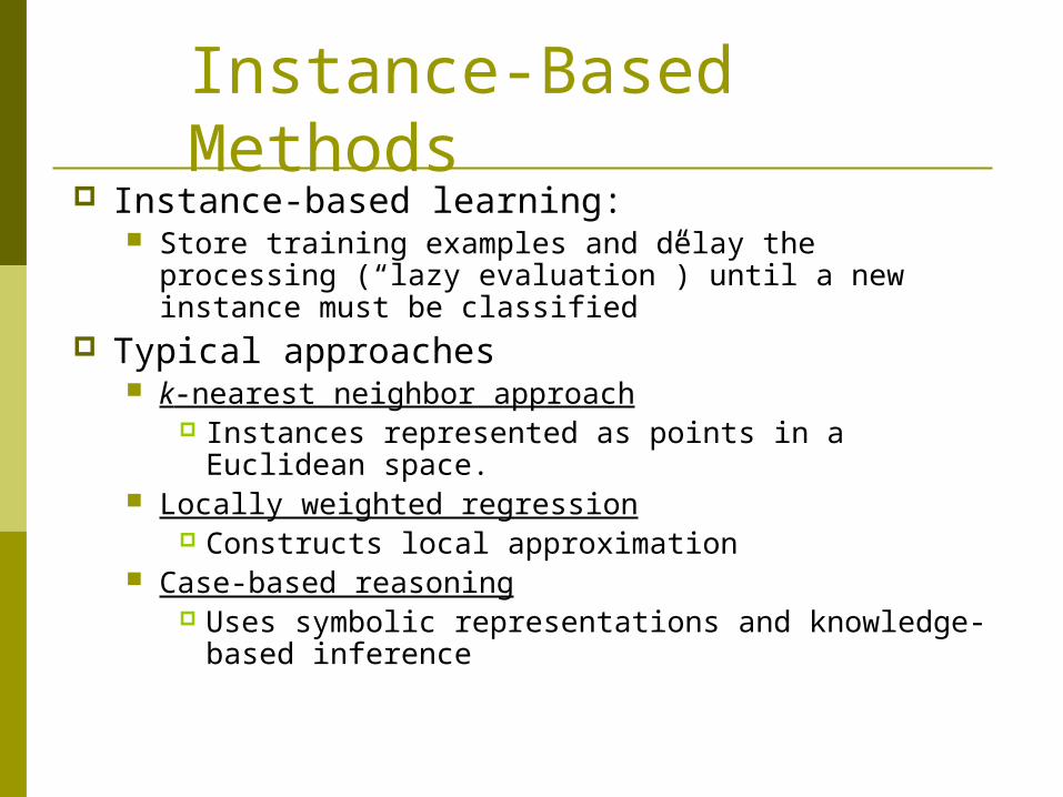
Instance-Based Methods

Instance-based learning: Store training examples and delay the processing

(“lazy evaluation”) until a new instance must be classified

Typical approaches k-nearest neighbor approach

Instances represented as points in a Euclidean space.

Locally weighted regression Constructs local approximation

Case-based reasoning Uses symbolic representations and knowledge-

based inference

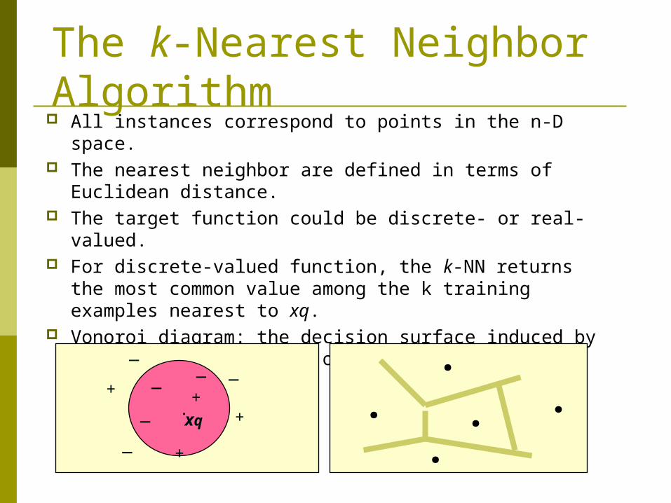
The k-Nearest Neighbor Algorithm

All instances correspond to points in the n-D space. The nearest neighbor are defined in terms of Euclidean

distance. The target function could be discrete- or real- valued. For discrete-valued function, the k-NN returns the most

common value among the k training examples nearest to xq.

Vonoroi diagram: the decision surface induced by 1-NN for a typical set of training examples.

.

_+

_ xq

+

_ _+

_

_

+

.

..

. .

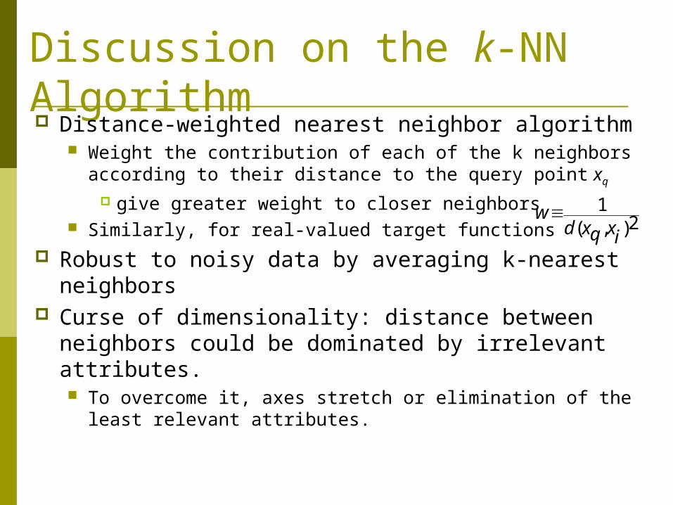
Discussion on the k-NN Algorithm Distance-weighted nearest neighbor algorithm

Weight the contribution of each of the k neighbors according to their distance to the query point xq

give greater weight to closer neighbors Similarly, for real-valued target functions

Robust to noisy data by averaging k-nearest neighbors

Curse of dimensionality: distance between neighbors could be dominated by irrelevant attributes. To overcome it, axes stretch or elimination of the least

relevant attributes.

wd xq xi

12( , )




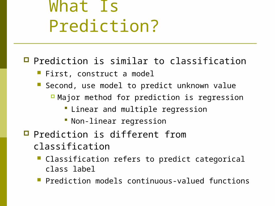
What Is Prediction?

Prediction is similar to classification First, construct a model Second, use model to predict unknown value

Major method for prediction is regression Linear and multiple regression Non-linear regression

Prediction is different from classification Classification refers to predict categorical class label Prediction models continuous-valued functions

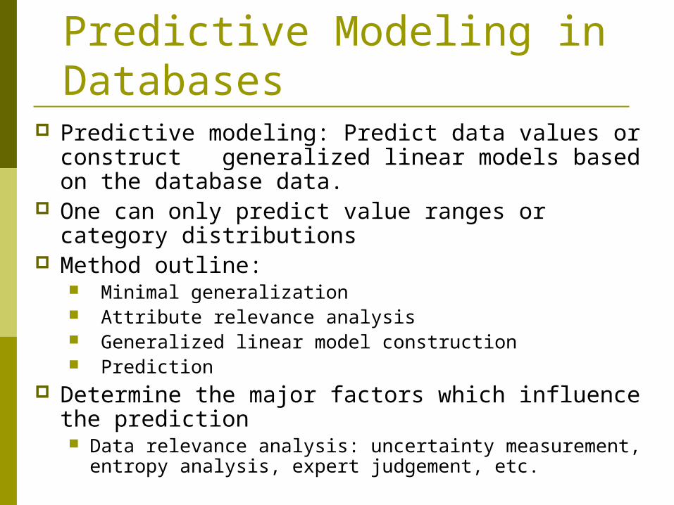
Predictive modeling: Predict data values or construct generalized linear models based on the database data.

One can only predict value ranges or category distributions

Method outline: Minimal generalization Attribute relevance analysis Generalized linear model construction Prediction

Determine the major factors which influence the prediction Data relevance analysis: uncertainty measurement,

entropy analysis, expert judgement, etc.

Predictive Modeling in Databases

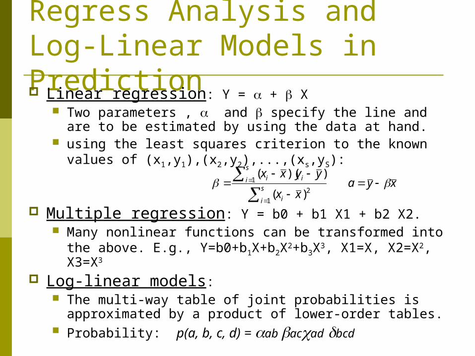
Regress Analysis and Log-Linear Models in Prediction Linear regression: Y = + X

Two parameters , and specify the line and are to be estimated by using the data at hand.

using the least squares criterion to the known values of (x1,y1),(x2,y2),...,(xs,yS):

Multiple regression: Y = b0 + b1 X1 + b2 X2. Many nonlinear functions can be transformed into the

above. E.g., Y=b0+b1X+b2X2+b3X3, X1=X, X2=X2, X3=X3

Log-linear models: The multi-way table of joint probabilities is approximated

by a product of lower-order tables. Probability: p(a, b, c, d) = ab acad bcd

s

i i

s

i ii

xx

yyxx

1

2

1

)(

))(( xya

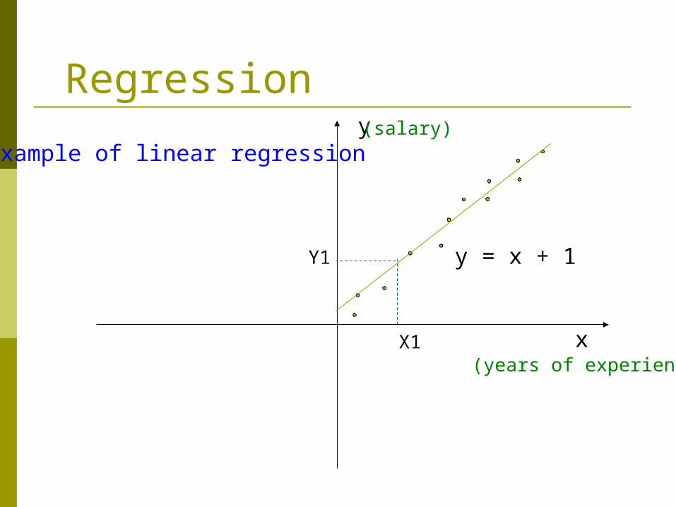
Regression

x

y

y = x + 1

X1

Y1

(salary)

(years of experience)

Example of linear regression




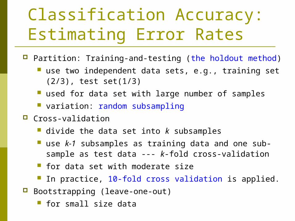
Classification Accuracy: Estimating Error Rates

Partition: Training-and-testing (the holdout method) use two independent data sets, e.g., training set (2/3),

test set(1/3) used for data set with large number of samples variation: random subsampling

Cross-validation divide the data set into k subsamples use k-1 subsamples as training data and one sub-sample

as test data --- k-fold cross-validation for data set with moderate size In practice, 10-fold cross validation is applied.

Bootstrapping (leave-one-out) for small size data

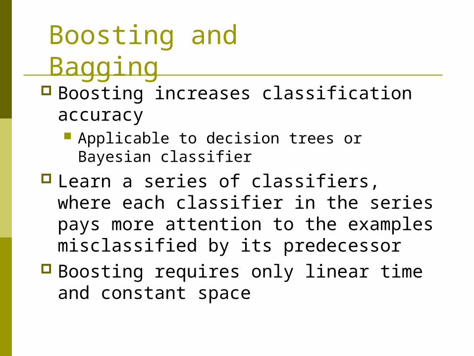
Boosting and Bagging

Boosting increases classification accuracy Applicable to decision trees or Bayesian

classifier Learn a series of classifiers, where each

classifier in the series pays more attention to the examples misclassified by its predecessor

Boosting requires only linear time and constant space

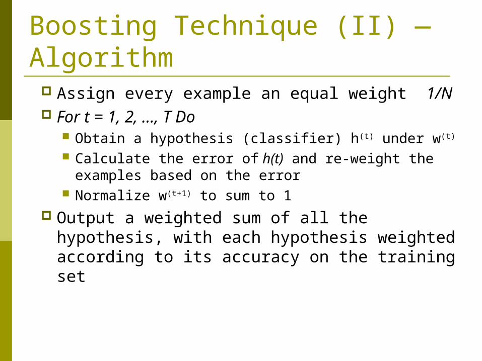
Boosting Technique (II) — Algorithm

Assign every example an equal weight 1/N For t = 1, 2, …, T Do

Obtain a hypothesis (classifier) h(t) under w(t)

Calculate the error of h(t) and re-weight the examples based on the error

Normalize w(t+1) to sum to 1 Output a weighted sum of all the

hypothesis, with each hypothesis weighted according to its accuracy on the training set

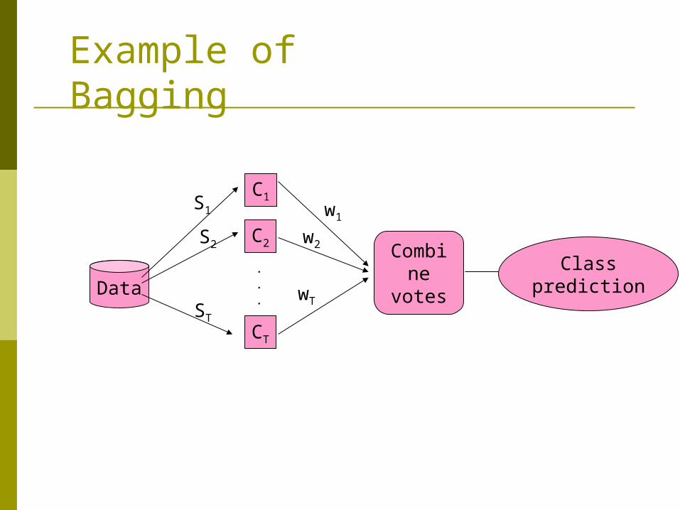
Example of Bagging

Data

C1

C2

CT

.

.

.

S1

S2

ST

w1

w2

wT

Combinevotes

Classprediction

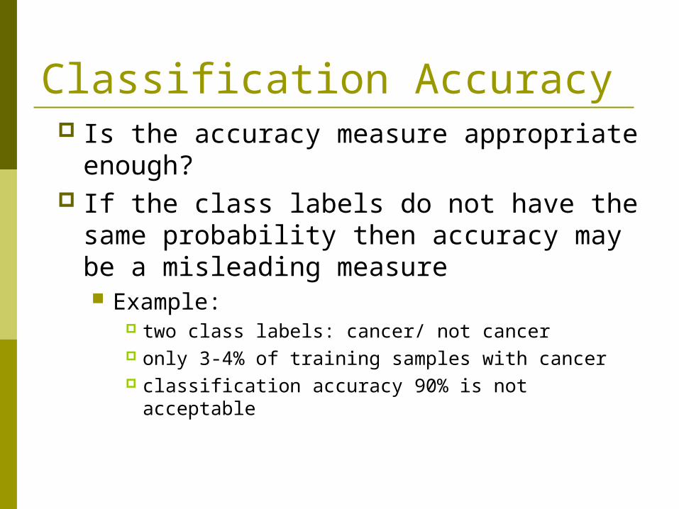
Classification Accuracy Is the accuracy measure appropriate

enough? If the class labels do not have the same

probability then accuracy may be a misleading measure Example:

two class labels: cancer/ not cancer only 3-4% of training samples with cancer classification accuracy 90% is not acceptable

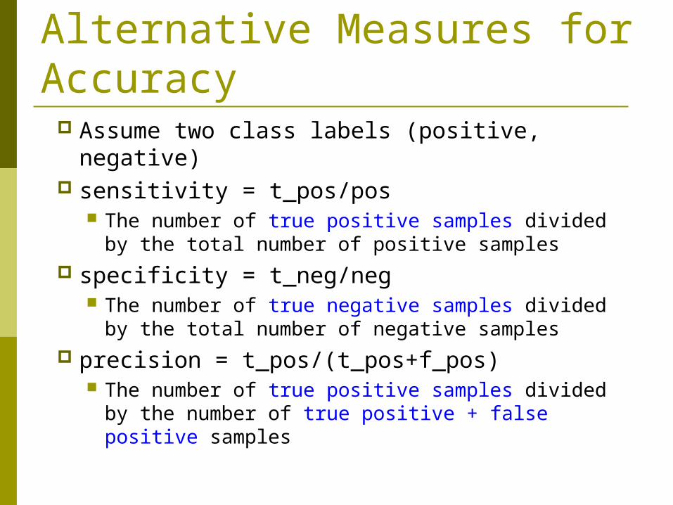
Alternative Measures for Accuracy

Assume two class labels (positive, negative) sensitivity = t_pos/pos

The number of true positive samples divided by the total number of positive samples

specificity = t_neg/neg The number of true negative samples divided by

the total number of negative samples precision = t_pos/(t_pos+f_pos)

The number of true positive samples divided by the number of true positive + false positive samples

Cases with samples belonging to more than one classes

In some cases a sample may belong to more than one class (overlapping classes)

In this case accuracy cannot be used to rate the classifier

The classifier instead of a class label returns a probability class distribution

Class prediction is considered correct if it agrees with first or second classifier’s guess

Documents

Classification and Prediction. What is classification? What is prediction? Issues regarding classification and prediction Classification by decision