Embed Size (px)
Citation preview
Discussion Papers
Statistics NorwayResearch department
No. 722 •December 2012
Edwin Leuven and Marte Rønning
Classroom grade composition and pupil achievement

Discussion Papers No. 722, December 2012 Statistics Norway, Research Department
Edwin Leuven and Marte Rønning
Classroom grade composition and pupil achievement
Abstract: This paper exploits discontinuous grade mixing rules in Norwegian junior high schools to estimate how classroom grade composition affects pupil achievement. Pupils in mixed grade classrooms are found to outperform pupils in single grade classrooms. This finding is driven by pupils benefiting from sharing the classroom with more mature peers from higher grades. The presence of lower grade peers is detrimental for achievement. Pupils can therefore benefit from de-tracking by grade, but the effects depend crucially on how the classroom is balanced in terms of lower and higher grades. These results reconcile the contradictory findings in the literature.
Keywords: educational production, combination classes, class size, peer effects
JEL classification: I2
Acknowledgements: We thank Adam Booij, Eric Bettinger, Julie Cullen, Monique De Haan, Pascaline Dupas, Tarjei Havnes, Magne Mogstad, Hessel Oosterbeek, Holger Sieg, David Sims and seminar participants for generous comments. A special thanks to Maria Fitzpatrick for providing us with descriptive statistics from SASS 2007. The usual disclaimer applies.
Address: Marte Rønning, Statistics Norway, Research Department. E-mail: [email protected]
Edwin Leuven, Department of Economics, University of Oslo. Also affiliated with the CEPR, CESifo, IZA and Statistics Norway. E-mail: [email protected]

Discussion Papers comprise research papers intended for international journals or books. A preprint of a Discussion Paper may be longer and more elaborate than a standard journal article, as it may include intermediate calculations and background material etc.
© Statistics Norway Abstracts with downloadable Discussion Papers in PDF are available on the Internet: http://www.ssb.no http://ideas.repec.org/s/ssb/dispap.html For printed Discussion Papers contact: Statistics Norway Telephone: +47 62 88 55 00 E-mail: [email protected] ISSN 0809-733X Print: Statistics Norway

3
Sammendrag
I denne artikkelen studerer vi betydningen av aldersblandede klasser på elevprestasjoner (målt som
eksamenskarakteren i 10. klasse) i ungdomsskolen. For å ta hensyn til at en klasses
alderssammensetning ikke er tilfeldig benytter vi Opplæringsloven paragraf 8.3 (som eksiterte til og
med skoleåret 2002/03) som legger sterke føringer på hvordan aldersblandede klasser skal settes
sammen.
Funnene viser at elever (som i løpet av ungdomsskolen) har vært i aldersblandede klasser presterer i
gjennomsnitt bedre enn elever som aldri har vært i aldersblandede klasser. Denne effekten er
sammensatt av en positiv effekt av å dele klasserom med eldre elever, og en negativ effekt av å dele
klasserom med yngre elever. Den positive effekten oppveier imidlertid den negative, noe som
forklarer hvorfor gjennomsnittseffekten er positiv. Elever kan altså tjene på å være i aldersblandede
klasser, men det er viktig å være klar over at effekten også avhenger av når man er blir eksponert for
eldre eller yngre elever.
1 Introduction
What are the consequences of classroom grade composition for pupil achievement? Many
children around the world find themselves in classrooms that group pupils from different
ages and/or grades. These combination classes are not only common in many poor
developing countries but are also often found in industrialized countries (Little, 2004).1 In
2007, about 28 percent of schools in the United States report "using multi-age grouping
to organize most classes or most pupils".2 Similarly, in 2001 about 25 percent of primary
school pupils were in mixed grade classrooms in Ontario (Fradette and Lataille-Démoré,
2003). The incidence of combination classes is also high in many European countries
(Mulryan-Kyne, 2005). In France, for example, 37 percent of primary school pupils are in
mixed grade classrooms.3
Although combination classes are sometimes advocated from an educational point
of view, they typically arise because of economic constraints. When confronted with an
increase or drop in enrollment, schools often group pupils from different grade levels to
avoid an extra (costly) classroom. This explains why combination classes are also common
in regular sized schools in cities, even though they are typically associated with small
schools in rural areas. Thirty-two percent of American public schools located in cities
report using multi-age grouping, compared to 26 percent in rural areas.
There are several ways in which combination classes can affect pupil achievement.
Classrooms constitute natural peer groups and grouping pupils from different grades in a
single classroom changes the peer group relative to a single grade classroom. This may
lead to direct negative or positive spillovers due to the presence of more or less able peers
since a pupil’s grade is positively correlated with her age and length of schooling, and
therefore with cognitive development and achievement (f.e. Bedard and Dhuey 2006;
Fredriksson and Öckert 2005; Leuven et al. 2010). In addition, peers from higher grades1Multi-grade and multi-age can correspond to different educational practices when age and grade do
not coincide. In most industrialized countries there is a close correspondence between age and grade, inwhich case the distinction bears little practical meaning.
2Based on the NCES Schools and Staffing Survey (SASS), a large sample survey of America’s elementaryand secondary schools.
3Personal communication with Ministère d’Éducation Nationale.
4
can serve as role models in terms of non-academic behavior, which can feed back to school
achievement. Finally, classrooms’ grade composition can also significantly affect teacher
inputs and teaching methods.
There is surprisingly little solid causal evidence about the impact of combination
classes on pupil achievement. Veenman (1995) surveyed 56 studies and concluded that
pupils in mixed grade classrooms do typically no worse and sometimes better than pupils
in classrooms that track pupils by grade. This conclusion was subsequently challenged by
Mason and Burns (1997) who argued that existing studies failed to address sorting of both
pupils and teachers into combination classes. This critique illustrates that any analysis of
the effectiveness of combination classes needs to address the same identification problems
as standard peer effects studies.
The lack of consensus about the effectiveness of combination classes reflects the
difficulty of giving quantitative measure to peer effects highlighted by Manski (1993).
To mitigate omitted variable bias most empirical peer-effects studies follow fixed-effect
type approaches that rely on within school or grade variation in peer characteristics (f.e.
Black et al. 2010; Hoxby 2000; Lavy et al. 2008; Ammermueller and Pischke 2009). This
strategy is compromised if pupils are not randomly allocated to peers and teachers (as in
Rothstein, 2010). Although an analysis at the grade rather than the classroom level may
partially address this issue, it can also lead to bias because peer group characteristics
are then subject to measurement error (Ammermueller and Pischke, 2009; Sojourner,
2008). A practical limitation of many fixed-effect type studies is that, by their nature,
they often have little variation in peer group composition. An alternative approach is to
rely on experiments which randomly allocate pupils to classes (Boozer and Cacciola, 2001;
Duflo et al., 2008). Social experiments are however rare and have their own limitations
(Heckman and Smith, 1995), and quasi-experiments are an interesting alternative (f.e.
Angrist and Lang 2004).
Some recent studies have addressed the endogeneity of combination classes. Sims
(2008) uses an instrumental variable approach and finds that a higher fraction of students
in combination classes negatively affects performance for 2nd and 3rd graders. Thomas
5

(2011) follows a fixed-effects and selection-on-observables approach to estimate the impact
of combination classes on 1st-graders and finds positive effects. Although these papers
do an arguably better job at correcting for selection bias than previous studies, their
contradictory findings remain a puzzle.
This paper sets out to estimate how classroom grade composition affects pupil achieve-
ment, and presents a number of significant contributions to the literature. First, we
use a novel identification approach that exploits institutional features in Norway that
significantly change the grade composition of classrooms. Norwegian junior high schools
are bound by national regulation that uses enrollment by grade level to determine class-
room grade composition. These rules determine predicted grade mixing which we use
as instruments for actual grade mixing. Second, the institutional features allows us to
both instrument for grade composition and class size. The third contribution of this study
is that we can separate the average effect of grade mixing into that of sharing the class
room with lower grades vs. higher grades.
To briefly summarize our results, we find that a one year exposure to a classroom that
combines two grade levels increases exam performance by about 9 percent of a standard
deviation. Further analysis shows that this effect is driven by pupils benefiting from
sharing the classroom with more mature peers from higher grades, whereas the presence
of a lower grade is detrimental to achievement. By the time they matriculate from junior
high school, most pupils in mixed grade classrooms in Norway have spend time with both
higher and lower grades. The average effect is therefore the sum of these positive and
negative effects. Since the positive effect of sharing the classroom with a higher grade
is somewhat larger in size that the negative effect of sharing the classroom with a lower
grade, the average effect is small and positive. This illustrates that, depending on the
type of exposure, average effects of grade mixing can be negative, positive or close to zero.
We argue below that these results go a long way toward explaining the contradictory
findings in the literature.
In what follows we start by describing the institutional context and our data sources.
After outlining our empirical approach in Section 4, we present our estimation results in
6

Section 5 and discuss how classroom age composition affects pupil achievement on the
short and longer term. Section 6 concludes.
2 Institutional settings and data
2.1 Institutions
Compulsory education in Norway consists of six years of primary school and three years
of junior high school education. Schools at the primary and secondary level are essentially
public — private schools amount for less than 3% of total enrollment — and there are no
school fees. Schools are governed at the local school district level and have catchment
areas, implying that parental school choice between schools for given residence is not
allowed.4
Children start primary school the year they turn seven.5 One defining feature of the
Norwegian schooling system is that early/late starting and grade retention are extremely
rare. In the current context this is important since we are interested in the effects of
classroom age composition on school achievement. Grade retention is strongly related to
maturity (e.g. Cahan and Cohen (1989)), and if schools practice grade retention then this
would introduce an extra endogenous margin of classrooms ability composition. As shown
in Bedard and Dhuey (2006) and Strøm (2004) however, there is no grade retention in
Norway. As a consequence nearly everybody starts junior high school the year they turn
fourteen.
Our analysis focuses on comprehensive schools that manage both a primary and junior
high school level (i.e. offer education from grade 1 to 9). More than half of the schools
in Norway are comprehensive, most of which are located outside the four major cities.6
Since these schools are relatively small, it is common practice to combine multiple grades
in a single classroom. All junior high schools in Norway — including the comprehensive4In specific cases parents can apply for exemptions to this rule, but this is very uncommon.5Of the pupils in our data about two percent did not start primary school they year they turned 7,
but one year earlier or later. School entry was lowered to age six as of 1997 when Norway increasedcompulsory schooling to 10 years. The official school starting age for the cohorts in our data was seven,and they had nine years of compulsory education.
6From the largest to the smallest these are: Oslo, Bergen, Trondheim and Stavanger. The last onehaving about 110,000 inhabitants at the time of our data.
7

schools — follow the same national curriculum, and all junior high school teachers are
required to have completed teacher college. This has the important advantage that none
of our results will be driven by differences in teacher education or curriculum.
2.2 Data
We use administrative enrollment data (provided by Statistics Norway) on all pupils
who graduated from junior high school in the school years 2001/02 and 2002/03. We
merge this data set with the school database GSI (“Grunnskolens Informasjonssystem”)
which, in addition to information on actual grade mixing, also contains information
on number of pupils and classes per grade at the start of the school year. Norwegian
administrative registers also provide us with information on the pupils’ birth date and
gender, socioeconomic characteristics such as mother’s and father’s education; whether
parents cohabit; and whether the pupil has a non-western migrant background.
As measures of pupil performance we use test-score data from both teacher set and
graded tests in the final year, and centralized exit exams (from Statistics Norway). At the
end of the final year in junior high, all pupils in Norway are required to take an exit exam.
Although the curriculum includes many subjects, a written exit exam is only undertaken
in one of three subjects: mathematics, Norwegian and English. The exams are centrally
assigned and it is not known in advance what the exam topic will be, and are therefore
beyond the control of schools, teachers and pupils. In the analysis we pool these three
subjects and standardize them with zero mean and standard deviation one. The teacher
tests as well as the exam scores are used to construct pupils’ junior high school exit test
scores which are important for secondary school choice. For students, both the exam and
teachers scores are therefore important because they are used for tracking decisions.
The correlation between the teacher score and the exam score is 0.8. Although both the
exam and teacher tests are supposed to measure learning of the same content (the junior
high school curriculum), there are some differences that can affect their comparability.
The exit exams are identical across schools and externally graded, which means that
there are no comparability issues across schools. The teacher grades in these subjects on
8
the other hand are based on tests set by students’ teachers. It is therefore less clear to
what extent these can be compared across schools. One advantage of the teacher tests
scores is that they are based on multiple evaluations, and are therefore probably less noisy
measures of achievement than the exam scores which are based on a single test. One
caveat regarding comparability arises if teachers engage in relative grading. This will
not only make the teacher test scores less comparable, but can also be a source of bias if
relative grading is affected by classrooms’ grade composition. Contrasting results based
on teacher tests and exam test can therefore tell us something about the importance of
relative grading. We will discuss these issues in more detail in the context of our results
below.
Grade mixing mostly occurs outside the major cities in comprehensive schools.7 We
therefore restrict our population of interest to these comprehensive schools outside the
four largest cities. Since classroom information is recorded at the grade level and pupils
are not necessarily randomly allocated to classrooms within a grade, we further restrict
our sample to schools that have one 7th grade class room when pupils start junior high
school. We drop 9 schools with missing information on predicted class size and schools
where information on grade mixing is lacking, and 90 pupils with missing information on
the exam score are also dropped.
Our analysis data set consists of 9,647 pupils and 388 schools. This amounts to about
10 percent of the pupil population and 1 out of 3 schools in Norway. In total 173 schools,
about 1 out 6 of all junior high schools, combine grades in at least one school year. Figure
A1 in the Appendix shows the location of the municipalities that have junior high schools
combining grades, as well as the comparison group of municipalities with small schools
that do not combine grades. The population of schools that we study not only represents
an important fraction of the overall school population in Norway, but also provides good
regional coverage.
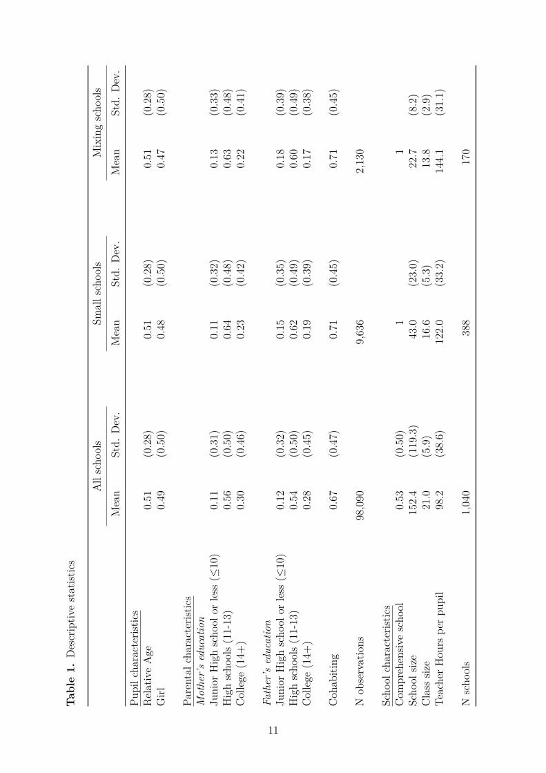
Table 1 reports descriptive statistics for the pupils in small schools, and compares
it to the total population of junior high school pupils. Relative age — which equals 07This means that it is not possible to do the analysis in schools that did not teach at the primary level.
9
for the youngest pupil (born December 31st) and 1 for the relatively oldest one (born
January 1st) — is on average 0.5. This implies that pupils in their final year of junior high
school in Norway are on average 16.5 years old. Differences with respect to individual
and parental characteristics are mostly small: Compared to the whole population, parents
of pupils in small schools are somewhat less educated, the mother and father are also
slightly more often cohabiting.
By construction larger differences are observed regarding the schools pupils are enrolled
in. First, schools are on average 3.5 times larger in the whole population compared to the
comprehensive schools outside the major cities that offer both primary and junior high
school education. Class size in these schools is also smaller, and teacher hours per pupil,
a common related measure for resource use, is larger. The table reports averages over
pupils’ time in junior high school.
When comparing the schools that mix grades to the reference population of small
schools we observe some differences with respect to parental background, but these tend to
be small and we cannot reject the null hypothesis that there are no difference (p=0.318).
Again, and — as we will show below — by virtue of the institutional rules, the mixing
schools are smaller with smaller classes.
3 Maximum class size rules
Junior high schools in Norway were subject to maximum class size rules (e.g. Leuven et al.,
2008). What makes these rules unique is that they sometimes interact in a systematic
fashion with classrooms’ grade composition. Section 8.3 of the Norwegian Education Act
(Opplæringsloven) stated the following:
1. A class in junior high school cannot have more than
(a) 30 pupils when there is one cohort in the class
(b) 24 pupils when there are two cohorts in the class
(c) 18 pupils when there are three cohorts in the class
10
Tab
le1.
Descriptiv
estatist
ics
Allscho
ols
Smalls
choo
lsMixingscho
ols
Mean
Std.
Dev.
Mean
Std.
Dev.
Mean
Std.
Dev.
Pupilc
haracterist
ics
RelativeAge
0.51
(0.28)
0.51
(0.28)
0.51
(0.28)
Girl
0.49
(0.50)
0.48
(0.50)
0.47
(0.50)
Parental
characteris
tics
Mother’seducation
Junior
Highscho
olor
less
(≤10)
0.11
(0.31)
0.11
(0.32)
0.13
(0.33)
Highscho
ols(11-13)
0.56
(0.50)
0.64
(0.48)
0.63
(0.48)
College
(14+
)0.30
(0.46)
0.23
(0.42)
0.22
(0.41)
Father’s
education
Junior
Highscho
olor
less
(≤10)
0.12
(0.32)
0.15
(0.35)
0.18
(0.39)
Highscho
ols(11-13)
0.54
(0.50)
0.62
(0.49)
0.60
(0.49)
College
(14+
)0.28
(0.45)
0.19
(0.39)
0.17
(0.38)
Coh
abiting
0.67
(0.47)
0.71
(0.45)
0.71
(0.45)
Nob
servations
98,090
9,636
2,130
Scho
olcharacteris
tics
Com
prehensiv
escho
ol0.53
(0.50)
11
Scho
olsiz
e152.4
(119.3)
43.0
(23.0)
22.7
(8.2)
Class
size
21.0
(5.9)
16.6
(5.3)
13.8
(2.9)
TeacherHou
rspe
rpu
pil
98.2
(38.6)
122.0
(33.2)
144.1
(31.1)
Nscho
ols
1,040
388
170
11

3 2 or 1
0
.2
.4
.6
.8
1Fr
actio
n w
ith 3
gra
des
in c
lass
room
10 18 50 100School size (Nr. of pupils in 7th-9th grade)
(a) Predicted
No grade mixing
Mix 2 grades
Mix 3 grades
0
.2
.4
.6
.8
1
Frac
tion
10 18 50 100School size (Nr. of pupils in 7th-9th grade)
(b) Actual, 7th grade
Figure 1. Classroom grade composition by school size
2. When there are multiple cohorts in a class, they need to be adjacent if possible
3. The school cannot simultaneously have mixed age and age-homogeneous classes
within the same grade level, or parallel mixed age classes
Schools are supposed to follow the Education Act. Rule 1(a) requires schools to open
an extra classroom if enrollment in a single grade classroom would exceed 30. This rule is
similar to the familiar Maimonides rule, exploited first by Angrist and Lavy (1999), and
for Norway by Leuven et al. (2008).
Where these rules are different is that they affect not only class size, but also class
grade composition. A school with no more than 18 pupils is therefore supposed to have a
single classroom with 3 cohorts. If enrollment is greater than 18, a school will need to
have two classrooms where one class will combine two grades as long as the combined
enrollment does not exceed 24. After this point, schools will are supposed to have only
single grade classrooms. Figure 1a illustrates this predicted grade mixing as a function of
school size. The decision whether to combine 3 grades in a classroom or not, depends
only on their combined enrollment not exceeding 18. Figure 1a therefore applies in the
same way for 7th, 8th and 9th grade.
Figure 1b shows the contemporaneous relationship between school size and multiple
grade classrooms that we observe in our data for 7th grade. The x-axis in Figure 1b is
on a logarithmic scale to improve the readability of the graph. The vertical line at 18
pupils marks the threshold above which schools are no longer supposed to combine all
12
three grades. There is a close relation between actual grade mixing and the grade mixing
rule. The propensity to combine three grades drops sharply by about 0.5 after school size
18. Where to the left of the first threshold schools essentially mixes all three grades, for
schools larger than 18 pupils the picture is somewhat more complicated and schools tend
to mix two adjacent grades. At first schools are bound by rules regarding the combination
of two adjacent grades, and for schools larger than 50 pupils there is no longer any grade
mixing taking place.
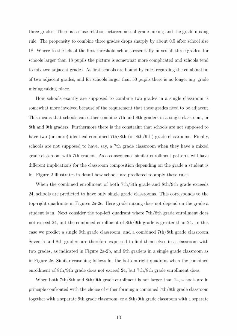
How schools exactly are supposed to combine two grades in a single classroom is
somewhat more involved because of the requirement that these grades need to be adjacent.
This means that schools can either combine 7th and 8th graders in a single classroom, or
8th and 9th graders. Furthermore there is the constraint that schools are not supposed to
have two (or more) identical combined 7th/8th (or 8th/9th) grade classrooms. Finally,
schools are not supposed to have, say, a 7th grade classroom when they have a mixed
grade classroom with 7th graders. As a consequence similar enrollment patterns will have
different implications for the classroom composition depending on the grade a student is
in. Figure 2 illustrates in detail how schools are predicted to apply these rules.
When the combined enrollment of both 7th/8th grade and 8th/9th grade exceeds
24, schools are predicted to have only single grade classrooms. This corresponds to the
top-right quadrants in Figures 2a-2c. Here grade mixing does not depend on the grade a
student is in. Next consider the top-left quadrant where 7th/8th grade enrollment does
not exceed 24, but the combined enrollment of 8th/9th grade is greater than 24. In this
case we predict a single 9th grade classroom, and a combined 7th/8th grade classroom.
Seventh and 8th graders are therefore expected to find themselves in a classroom with
two grades, as indicated in Figure 2a-2b, and 9th graders in a single grade classroom as
in Figure 2c. Similar reasoning follows for the bottom-right quadrant when the combined
enrollment of 8th/9th grade does not exceed 24, but 7th/8th grade enrollment does.
When both 7th/8th and 8th/9th grade enrollment is not larger than 24, schools are in
principle confronted with the choice of either forming a combined 7th/8th grade classroom
together with a separate 9th grade classroom, or a 8th/9th grade classroom with a separate
13

12
1
2 1
1024
40N
r of p
upils
in 8
th +
9th
gra
de
10 24 40Nr of pupils in 7th + 8th grade
(a) For 7th graders
22
2
2 1
1024
40N
r of p
upils
in 8
th +
9th
gra
de10 24 40
Nr of pupils in 7th + 8th grade
(b) For 8th graders
21
2
1 1
1024
40N
r of p
upils
in 8
th +
9th
gra
de
10 24 40Nr of pupils in 7th + 8th grade
(c) For 9th graders
Figure 2. Predicted grade mixing by grade level when school size > 18
7th grade classroom. We predict that schools try to keep the combined classroom as
small as possible, and therefore choose for a separate 7th grade classroom (rather than a
9th grade classroom) if there are more 7th than 9th graders. This means that above the
diagonal in the bottom-left quadrant – where there are as many 7th as 9th graders – we
predict to see a combined 7th/8th grade classroom and below the diagonal a combined
8th/9th grade classroom.
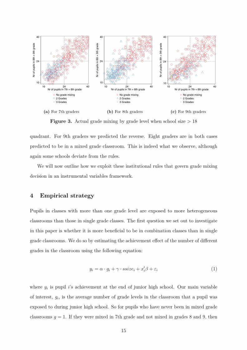
Figure 3 shows actual grade mixing as a function of the relevant cohort sizes, and
how schools go from a double to a single grade classrooms. Most schools find themselves
in either the top-right or bottom-left quadrant. In the top-right quadrant the rules
stipulate that grades are not to be combined which is indeed what we observe in the data,
with a few exceptions these are all regular single grade classrooms. In the bottom-left
quadrant schools are predicted to combine two grades. Again, schools do not always
follows the rules, but as predicted we see that 7th graders are more likely to be in a
mixed classroom above the diagonal when 9th grade enrollment is larger than 7th grade
enrollment. Similarly we see 9th graders more often in a combined classroom below the
diagonal. Lastly, and consistent with the rest, 8th graders are typically in a mixed grade
classroom when enrollment puts a school in the bottom-left quadrant.
In the top-left and bottom-right quadrants we predicted different grade mixing depend-
ing on the grade students are in. Seventh graders are predicted to be in a mixed grade
classroom in the top-left quadrant and in a single grade classroom in the bottom-right
14
10
24
40N
r of p
upils
in 8
th +
9th
gra
de
10 24 40Nr of pupils in 7th + 8th grade
No grade mixing2 Grades3 Grades
(a) For 7th graders
10
24
40
Nr o
f pup
ils in
8th
+ 9
th g
rade
10 24 40Nr of pupils in 7th + 8th grade
No grade mixing2 Grades3 Grades
(b) For 8th graders
10
24
40
Nr o
f pup
ils in
8th
+ 9
th g
rade
10 24 40Nr of pupils in 7th + 8th grade
No grade mixing2 Grades3 Grades
(c) For 9th graders
Figure 3. Actual grade mixing by grade level when school size > 18
quadrant. For 9th graders we predicted the reverse. Eight graders are in both cases
predicted to be in a mixed grade classroom. This is indeed what we observe, although
again some schools deviate from the rules.
We will now outline how we exploit these institutional rules that govern grade mixing
decision in an instrumental variables framework.
4 Empirical strategy
Pupils in classes with more than one grade level are exposed to more heterogeneous
classrooms than those in single grade classes. The first question we set out to investigate
in this paper is whether it is more beneficial to be in combination classes than in single
grade classrooms. We do so by estimating the achievement effect of the number of different
grades in the classroom using the following equation:
yi = α · gi + γ · ssizei + x′iβ + εi (1)
where yi is pupil i’s achievement at the end of junior high school. Our main variable
of interest, gi, is the average number of grade levels in the classroom that a pupil was
exposed to during junior high school. So for pupils who have never been in mixed grade
classrooms g = 1. If they were mixed in 7th grade and not mixed in grades 8 and 9, then
15
g = (2 + 1 + 1)/3 = 4/3, etc. Given the policy that we study — which acts on the raw
number of grades in the classroom as illustrated by the graphs above — this is a natural
parametrization. Since the policy changes the raw number of grades, estimating the effect
of the raw number of grades therefore delivers policy relevant average effects. We also
add school and family control variables in xi, which include parental education, whether
parents are living together, pupils gender and relative age.8
As documented above, grade mixing is governed by the rules set by the Ministry of
Education, but endogeneity is potentially an issue, especially close to the thresholds where
schools more often deviate from the rules. One example of endogenous grade mixing arises
when school’s grade mixing in year t depends on the (perceived) success of grade mixing
in year t− 1, rather than the rule.
We follow an instrumental variable approach in the spirit of Angrist and Lavy (1999),
and use the predicted grade mixing documented in Figures 1a and 2 to construct instru-
ments for actual grade mixing to take any remaining endogeneity into account. More in
particular, using the enrollment of 7th, 8th and 9th graders in a given school year we
can determine the predicted grade mixing according to the rules. For each student i we
calculate the predicted grade mixing separately for each grade level j when she was in
junior high school. Predicted grade mixing for student i in grade j, E[gij], is defined in
Table 2 where njit is the number of j-th graders in student i’s school in year t.
In our 2SLS estimation we use six predicted grade mixing dummies, one for each grade
and value of E[gij ], leaving out the reference group of no grade mixing. The first stage for
average grade mixing in junior high school thus becomes
gi =9∑
j=7
3∑n=2
δjn1[E[gij ]=n] + δs · ssizei + x′iδx + ui (2)
We control throughout for school size (ssizei), the combined enrollment of 7th, 8th and
9th grade, when the pupil started junior high school. School size can be thought of as a8Relative age = (1 - day of birth) / 364, so that the relatively oldest pupil has age 1 and the youngest
age 0. We also estimated specifications where we instrument actual age using relative age as in Bedardand Dhuey 2006; Black et al. 2010. This does not affect our results. We report estimation results fromreduced form models with respect to age for simplicity.
16
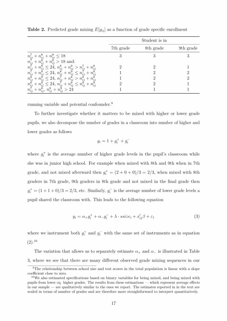
Table 2. Predicted grade mixing E[gij] as a function of grade specific enrollment
Student is in7th grade 8th grade 9th grade
n7ij + n8
ij + n9ij ≤ 18 3 3 3
n7ij + n8
ij + n9ij > 18 and:
n7ij + n8
ij ≤ 24, n8ij + n9
ij > n7ij + n8
ij 2 2 1n7
ij + n8ij ≤ 24, n8
ij + n9ij ≤ n7
ij + n8ij 1 2 2
n8ij + n9
ij ≤ 24, n7ij + n8
ij > n8ij + n9
ij 1 2 2n8
ij + n9ij ≤ 24, n7
ij + n8ij ≤ n8
ij + n9ij 2 2 1
n7ij + n8
ij, n8ij + n9
ij > 24 1 1 1
running variable and potential confounder.9
To further investigate whether it matters to be mixed with higher or lower grade
pupils, we also decompose the number of grades in a classroom into number of higher and
lower grades as follows
gi = 1 + g+i + g−i
where g+i is the average number of higher grade levels in the pupil’s classroom while
she was in junior high school. For example when mixed with 8th and 9th when in 7th
grade, and not mixed afterward then g+i = (2 + 0 + 0)/3 = 2/3, when mixed with 8th
graders in 7th grade, 9th graders in 8th grade and not mixed in the final grade then
g+i = (1 + 1 + 0)/3 = 2/3, etc. Similarly, g−i is the average number of lower grade levels a
pupil shared the classroom with. This leads to the following equation
yi = α+g+i + α−g
−i + λ · ssizei + x′ijβ + ε1 (3)
where we instrument both g+i and g−i with the same set of instruments as in equation
(2).10
The variation that allows us to separately estimate α+ and α− is illustrated in Table
3, where we see that there are many different observed grade mixing sequences in our9The relationship between school size and test scores in the total population is linear with a slope
coefficient close to zero.10We also estimated specifications based on binary variables for being mixed, and being mixed with
pupils from lower cq. higher grades. The results from these estimations — which represent average effectsin our sample — are qualitatively similar to the ones we report. The estimates reported in in the text arescaled in terms of number of grades and are therefore more straightforward to interpret quantitatively.
17
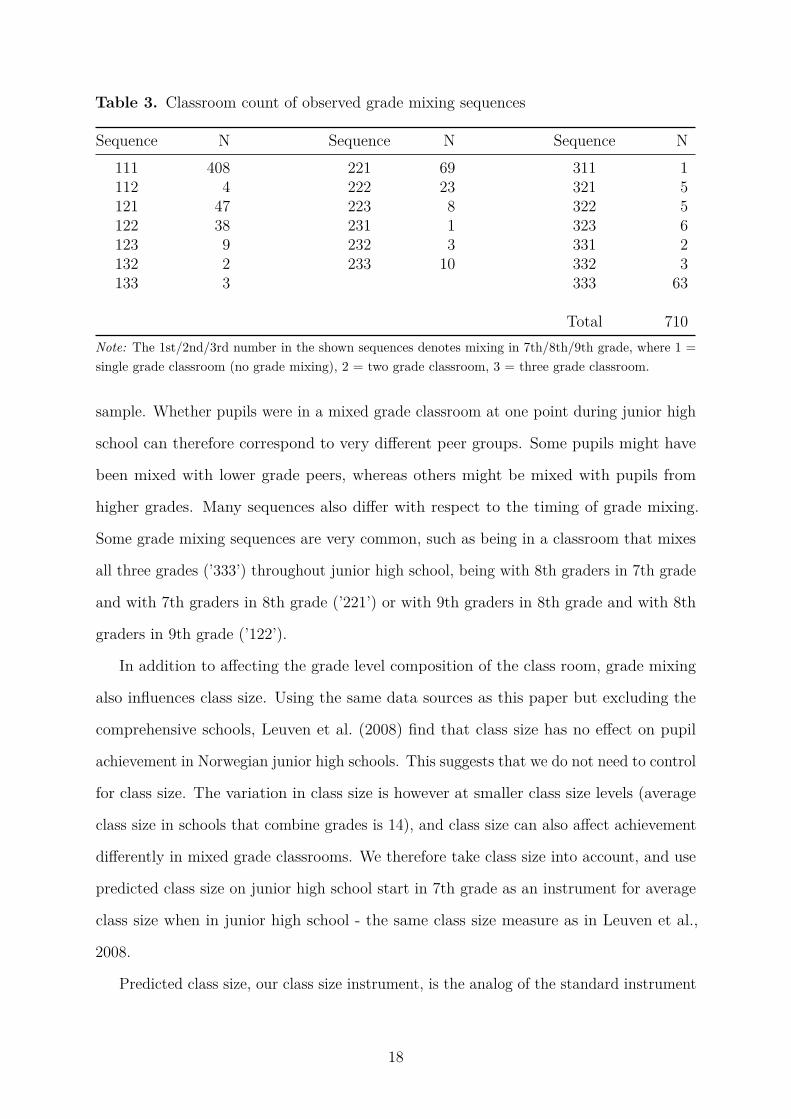
Table 3. Classroom count of observed grade mixing sequences
Sequence N Sequence N Sequence N111 408 221 69 311 1112 4 222 23 321 5121 47 223 8 322 5122 38 231 1 323 6123 9 232 3 331 2132 2 233 10 332 3133 3 333 63
Total 710Note: The 1st/2nd/3rd number in the shown sequences denotes mixing in 7th/8th/9th grade, where 1 =single grade classroom (no grade mixing), 2 = two grade classroom, 3 = three grade classroom.
sample. Whether pupils were in a mixed grade classroom at one point during junior high
school can therefore correspond to very different peer groups. Some pupils might have
been mixed with lower grade peers, whereas others might be mixed with pupils from
higher grades. Many sequences also differ with respect to the timing of grade mixing.
Some grade mixing sequences are very common, such as being in a classroom that mixes
all three grades (’333’) throughout junior high school, being with 8th graders in 7th grade
and with 7th graders in 8th grade (’221’) or with 9th graders in 8th grade and with 8th
graders in 9th grade (’122’).
In addition to affecting the grade level composition of the class room, grade mixing
also influences class size. Using the same data sources as this paper but excluding the
comprehensive schools, Leuven et al. (2008) find that class size has no effect on pupil
achievement in Norwegian junior high schools. This suggests that we do not need to control
for class size. The variation in class size is however at smaller class size levels (average
class size in schools that combine grades is 14), and class size can also affect achievement
differently in mixed grade classrooms. We therefore take class size into account, and use
predicted class size on junior high school start in 7th grade as an instrument for average
class size when in junior high school - the same class size measure as in Leuven et al.,
2008.
Predicted class size, our class size instrument, is the analog of the standard instrument
18
that is used in the class size literature and is defined as follows
E[csizei] = n7i7 + (n8
i7 + n9i7) · 1[E[gi7]=3] + 0.5n8
i7 · 1[E[gi7]=2] (4)
Equation (4) implies that the expected class size on junior high school start is n7i7 in
a single grade class, and n7i7 + n8
i7 + n9i7 in a three grade class. When two grades are
predicted to be combined this can either be 7th and 8th grade or 8th and 9th grade. In
the first case the expected class size is n7i7 + n8
i7, and in the second case n7i7. We assume
that these events have equal probability (0.5) which gives the expected class size in (4).
The class size effect is therefore identified through an interaction between the predicted
grade mixing rules and adjacent cohort sizes.
Since we are instrumenting class size we will estimate an additional first-stage for class
size and augment the first stage (2), and the first-stages for g+i and g−i with (4). Our
results below confirm our earlier findings for larger schools in Leuven et al. (2008), namely
that there is no evidence of significant class size effects in Norwegian lower secondary
schools. Our effect estimates of grade composition therefore do not change when we do
not control for class size.
With a single discontinuity it would not be possible to separately estimate grade
mixing and class size effects. The rules generate however many discontinuities. We can
separate the grade mixing and class size effects because — for a given drop in class size
— these discontinuities differ in the way they affect classrooms’ grade composition. The
grade mixing and class size effects are therefore identified by pooling the discontinuities
and relying on homogeneity of the class size effect across discontinuities. In our setup this
is essentially achieved by the separable specification (which one can also think of as a first
order Taylor expansion of the underlying structural function).
The first stages we report below show that in practice the grade mixing and class size
effects are well identified in the data. The class size instrument almost exclusively loads
on class size, and the mixing instruments almost exclusively on grade mixing. That our
specification is reasonable is supported by our results which are extremely robust: The
estimated grade mixing effects are essentially unchanged (i) with and without controlling
19

for class size, and (ii) with and without instrumenting for class size. Moreover, the
coefficient on class size is insignificant and extremely small. Including fixed effects does
not change this result. It is hard to think of a scenario where class size is an important
omitted variable that biases our grade mixing estimates, but that gives us zero class size
effects and unchanged grade mixing effects in the wide range of specifications that we
report.
Because we exploit the rules documented above as instrumental variables, we investigate
their validity in two ways. First we check whether parents and/or schools position
themselves in non-random ways around the points where schools are supposed to change the
classroom grade composition. A second concern is that there are alternative confounding
changes of related school inputs. We discuss each in turn.
4.1 Sorting
We can distinguish between two main sources of sorting. The first is supply side sorting
which arises when school or local education authorities manipulate enrollment relative to
the discontinuities. The main reason for doing so is typically related to funding. In some
countries, for example in Sweden, local education authorities are known to sometimes
redraw school catchment areas in such a way as to avoid opening a new classroom when
maximum class-size rules would dictate this. This is however not an issue here since
catchment areas are fixed in Norway.
The second potential source of sorting comes from the demand side. When parents
prefer mixing or non-mixing classrooms they might decide to enroll their children in a
different school. If for example more advantaged families sort in different ways than
disadvantaged families, the underlying pupil population at both sides of the discontinuities
are no longer comparable. The implicit exclusion restriction in the IV design then breaks
down and we would no longer recover reliable estimates. A striking example of sorting
was reported in Urquiola and Verhoogen (2009) for Chile. In an earlier class-size study
(Leuven et al., 2008) we did not find any similar evidence for Norway. When it comes to
institutional sorting this is as expected since catchment areas are fixed.
20
0
.01
.02
.03D
ensi
ty
0 50 100 150Nr. of 7th-9th graders at start of Jr. High School
Note: Discontinuity estimate (log difference in height): 0.16 (0.19)
(a) Pooled 7th, 8th & 9th grade enrollment
0
.01
.02
.03
.04
Den
sity
0 20 40 60 80Nr. of 7th & 8th graders at start of Jr. High School
Note: Discontinuity estimate (log difference in height): 0.38 (0.24)
(b) Pooled 7th & 8th grade
0
.01
.02
.03
.04
.05
Den
sity
0 20 40 60 80 100Nr. of 8th & 9th graders at start of Jr. High School
Note: Discontinuity estimate (log difference in height): -0.05 (0.25)
(c) Pooled 8th & 9th grade enrollment
Figure 4. Density checks21
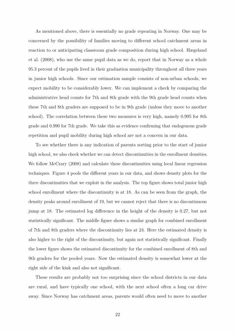
As mentioned above, there is essentially no grade repeating in Norway. One may be
concerned by the possibility of families moving to different school catchment areas in
reaction to or anticipating classroom grade composition during high school. Hægeland
et al. (2008), who use the same pupil data as we do, report that in Norway as a whole
95.3 percent of the pupils lived in their graduation municipality throughout all three years
in junior high schools. Since our estimation sample consists of non-urban schools, we
expect mobility to be considerably lower. We can implement a check by comparing the
administrative head counts for 7th and 8th grade with the 9th grade head counts when
these 7th and 8th graders are supposed to be in 9th grade (unless they move to another
school). The correlation between these two measures is very high, namely 0.995 for 8th
grade and 0.990 for 7th grade. We take this as evidence confirming that endogenous grade
repetition and pupil mobility during high school are not a concern in our data.
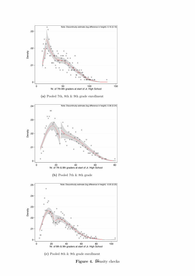
To see whether there is any indication of parents sorting prior to the start of junior
high school, we also check whether we can detect discontinuities in the enrollment densities.
We follow McCrary (2008) and calculate these discontinuities using local linear regression
techniques. Figure 4 pools the different years in our data, and shows density plots for the
three discontinuities that we exploit in the analysis. The top figure shows total junior high
school enrollment where the discontinuity is at 18. As can be seen from the graph, the
density peaks around enrollment of 19, but we cannot reject that there is no discontinuous
jump at 18. The estimated log difference in the height of the density is 0.27, but not
statistically significant. The middle figure shows a similar graph for combined enrollment
of 7th and 8th graders where the discontinuity lies at 24. Here the estimated density is
also higher to the right of the discontinuity, but again not statistically significant. Finally
the lower figure shows the estimated discontinuity for the combined enrollment of 8th and
9th graders for the pooled years. Now the estimated density is somewhat lower at the
right side of the kink and also not significant.
These results are probably not too surprising since the school districts in our data
are rural, and have typically one school, with the next school often a long car drive
away. Since Norway has catchment areas, parents would often need to move to another
22

municipality in order to enroll their child in another school. They would need to find
new employment or face a long commute, and the economic and social cost of sorting is
therefore probably very high.
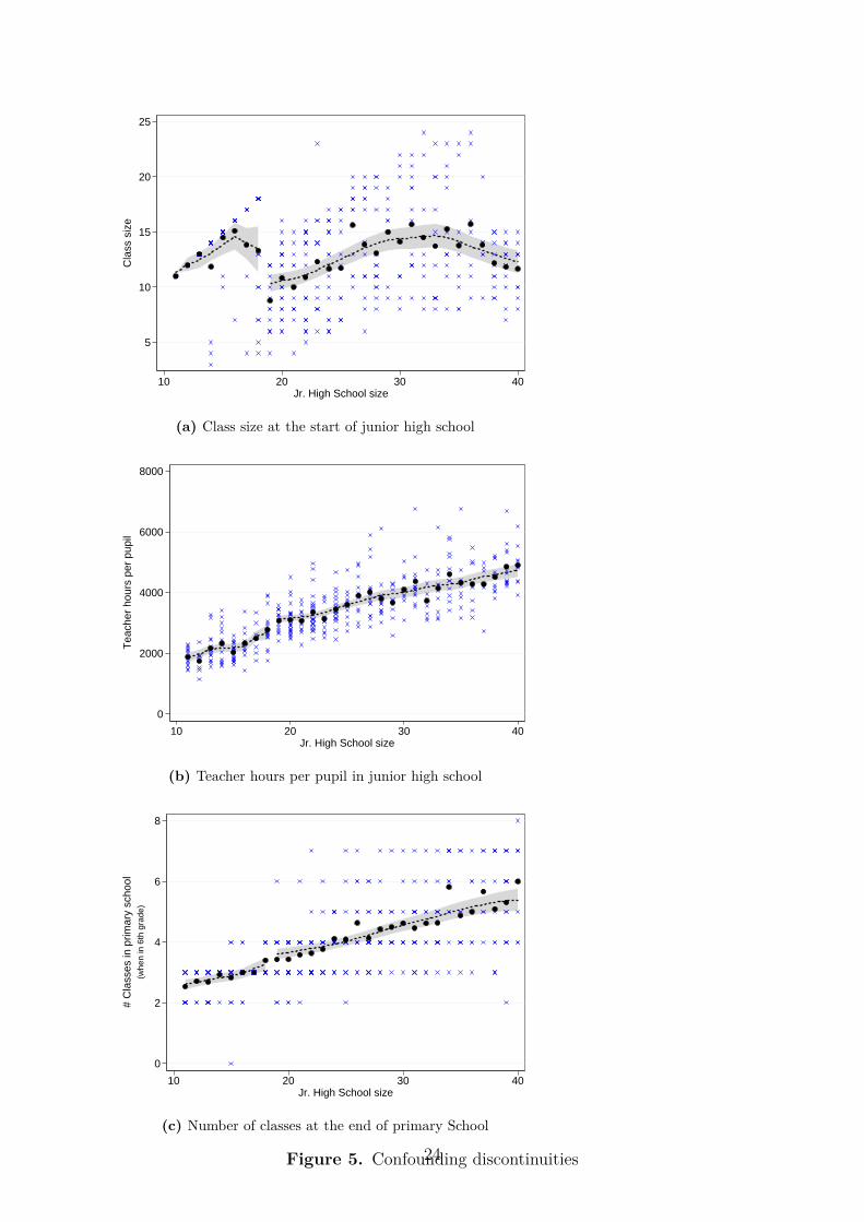
4.2 Confounding discontinuities
Class size/pupil-teacher ratio Although we do not find any evidence of sorting, we
know that class size discontinuously changes when combining grades. The reason is of
course that, keeping enrollment fixed, combining grades involves less classrooms and
therefore mechanically larger classes. This is illustrated in Figure 5a which plots the data
points corresponding to the schools in our sample and a smoothed regression line and
bootstrapped confidence interval at both sides of the discontinuity. Since we are interested
in estimating the causal effect of changing the classroom grade composition, we need to
keep the pupil-teacher ratio constant. This implies that we need to control for class size
in our specifications.
From our administrative data we know the ratio of teacher hours per pupil at the
junior high school level. Figure 5b shows that the drop in class-size does not seem to
be accompanied by a drop in teacher hours per pupil. This suggests that when schools
combine grades and have larger classes, input in terms of teacher time remains constant.
This would remove the need to control for class size in order to estimate the ceteris paribus
effect of changing classroom grade composition. The results of Leuven et al. (2008) also
suggest that there is no need to control for class size — although for a different reason —
since they did not find evidence that class size affects achievement in Norwegian junior
high schools and can rule out small effects.
The population of schools in the current paper is however different and also the variation
in class-size is at smaller class size levels than in Leuven et al. (2008). Furthermore, we are
also not certain that teacher hours are indeed balanced in the classrooms that we compare
because, our data does not allow us to link teachers to classrooms. To address these
concerns we control for class-size when estimating how grade mixing affects achievement.
As discussed above, when we control for class-size, it is instrumented with predicted
23
5
10
15
20
25C
lass
siz
e
10 20 30 40Jr. High School size
(a) Class size at the start of junior high school
0
2000
4000
6000
8000
Tea
cher
hou
rs p
er p
upil
10 20 30 40Jr. High School size
(b) Teacher hours per pupil in junior high school
0
2
4
6
8
10 20 30 40Jr. High School size
(whe
n in
6th
gra
de)
# C
lass
es in
prim
ary
scho
ol
(c) Number of classes at the end of primary School
Figure 5. Confounding discontinuities24
class-size at the start of junior high school as in Angrist and Lavy (1999). It turns out that
the estimated effects of grade composition are insensitive to whether or not we control for
class size. Moreover, we do not find evidence of class size effects. This is consistent with
the balancing of teacher hours shown in Figure 5b.
Finally, one may be concerned that there is an independent effect of the number of
teachers present in the classroom conditional on teacher hours per pupil. Although we
cannot rule this out, previous research from the Tennessee STAR experiment did not find
that having a teaching aide in the classroom improved student outcomes (f.e. Krueger,
1999).
Classroom composition in primary school In primary school, pupils from different grades
can also be combined in a single classroom. These rules are however different from those in
junior high school (both in terms of thresholds, but also in that they rely on different and
more cohorts simultaneously). One might nevertheless be concerned that grade mixing in
junior high school correlates with grade mixing in primary school. Since combining grades
changes the number of classes we verify whether we observe a discontinuous change in the
number of classes when the pupil was in 6th grade (the final grade of primary school).
Figure 5c shows that there is no evidence of such a confounding discontinuity.11
5 The effect of class room grade composition on achievement
This section presents the outcomes of our analysis. We start out by considering average
effects of classroom grade composition on exam scores at the end of junior high school.
After these overall results we present separate effect estimates for boys and girls.
5.1 Exam scores
The results from estimating equation (1) by OLS are shown in the first two columns of
Table 5. The first column is a simple regression of standardized exam scores on average
classroom grade composition during junior high school. This shows that pupils who have11An analysis of grade mixing in primary is not possible because we cannot reconstruct the complete
grade mixing histories for our cohorts, and there are no test scores available at the primary level.
25
been in classes with one more grade level in their class during junior high school perform
approximately 6 percent of a standard deviation better on the exam. The second column
adds class size, school size, and our family background characteristics. The effect of
number of grades increases somewhat to an effect size of 7 percent and remains significant
at the 10 percent level.
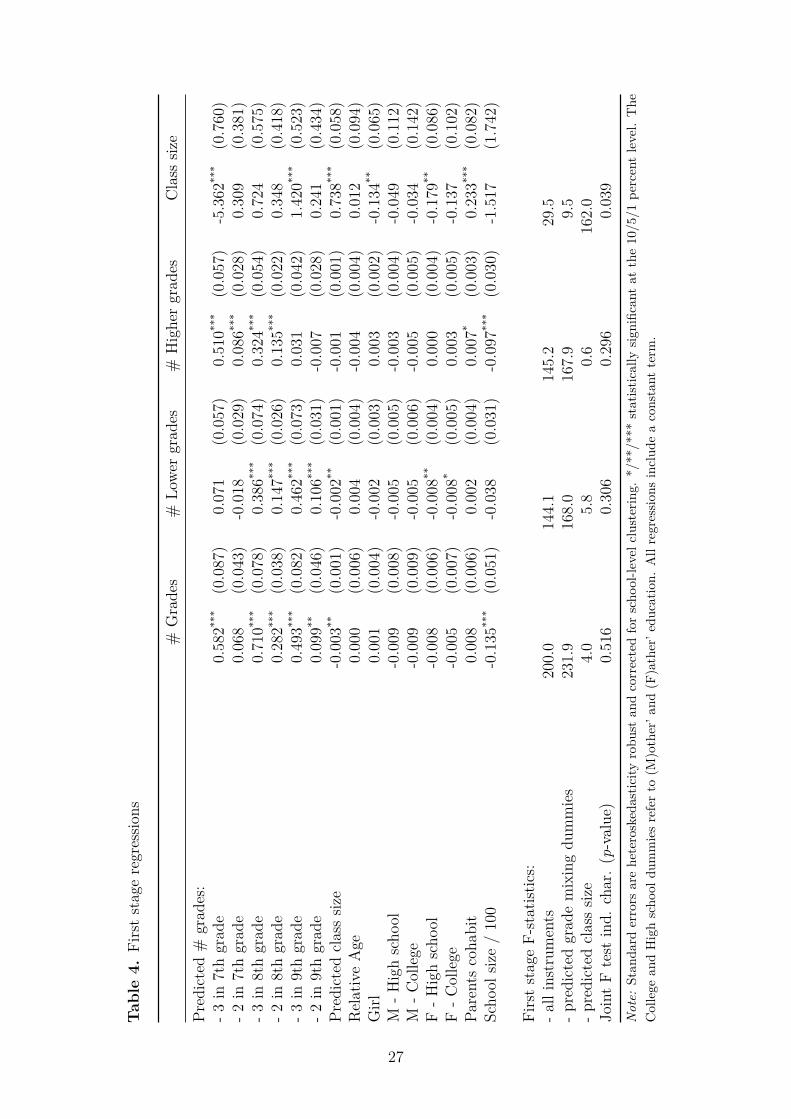
The second to fourth column in Table 5 present the estimates after instrumenting
number of grade levels in the classroom using 2SLS for various class-size specifications.
Table 4 reports the first-stage results. When we test the joint significance of our instru-
ments, the predicted grade level dummies, we obtain an F-statistic equal to 232. The
third column reports a statistically significant 2SLS estimate of 0.092 of the number of
grades in a class room on achievement without controlling for class size. This is somewhat
higher than the comparable OLS estimate in the first column. The second 2SLS estimate
assumes that class size is exogenous. The point estimate is 0.095 and therefore essentially
unchanged compared to the specification without class-size. This result does not change
when we also instrument class size in the final column.
The estimated effect of class size is very small and positive, 0.002, insignificant yet
precisely estimated. The results in Table 5 show that not only are there no confounding
effects of class size on the number of grade levels in class, but also confirm the earlier
finding of Leuven et al. (2008) that class size effects in Norwegian junior high schools are
negligible.
Turning to the control variables we see that the oldest pupils in the cohort, born in
January, score about 16 percent of a standard deviation higher than the youngest in the
cohort born in December. Girls also score significantly higher than boys, and exam scores
are also better for children of higher educated and cohabiting parents. Finally, we see
that there is no statistically significant relation between the running variable, school size,
and exam scores (dropping school size from our regressions does not affect the results).
These results might be surprising, in the sense that the heterogeneity of the classroom
increases when combining grades. The results of Duflo et al. (2008) for Kenya for example
suggest that this should have deteriorated pupils’ achievement. To gain more insight into
26
Tab
le4.
Firststageregressio
ns
#Grades
#Lo
wergrad
es#
Highergrad
esClass
size
Predicted#
grad
es:
-3in
7thgrad
e0.582**
*(0.087)
0.071
(0.057)
0.510**
*(0.057)
-5.362
***
(0.760)
-2in
7thgrad
e0.068
(0.043)
-0.018
(0.029)
0.086**
*(0.028)
0.309
(0.381)
-3in
8thgrad
e0.710**
*(0.078)
0.386**
*(0.074)
0.324**
*(0.054)
0.724
(0.575)
-2in
8thgrad
e0.282**
*(0.038)
0.147**
*(0.026)
0.135**
*(0.022)
0.348
(0.418)
-3in
9thgrad
e0.493**
*(0.082)
0.462**
*(0.073)
0.031
(0.042)
1.420**
*(0.523)
-2in
9thgrad
e0.099**
(0.046)
0.106**
*(0.031)
-0.007
(0.028)
0.241
(0.434)
Predictedclasssiz
e-0.003
**(0.001)
-0.002
**(0.001)
-0.001
(0.001)
0.738**
*(0.058)
RelativeAge
0.000
(0.006)
0.004
(0.004)
-0.004
(0.004)
0.012
(0.094)
Girl
0.001
(0.004)
-0.002
(0.003)
0.003
(0.002)
-0.134
**(0.065)
M-H
ighscho
ol-0.009
(0.008)
-0.005
(0.005)
-0.003
(0.004)
-0.049
(0.112)
M-C
ollege
-0.009
(0.009)
-0.005
(0.006)
-0.005
(0.005)
-0.034
(0.142)
F-H
ighscho
ol-0.008
(0.006)
-0.008
**(0.004)
0.000
(0.004)
-0.179
**(0.086)
F-C
ollege
-0.005
(0.007)
-0.008
*(0.005)
0.003
(0.005)
-0.137
(0.102)
Parentscoha
bit
0.008
(0.006)
0.002
(0.004)
0.007*
(0.003)
0.233**
*(0.082)
Scho
olsiz
e/100
-0.135
***
(0.051)
-0.038
(0.031)
-0.097
***
(0.030)
-1.517
(1.742)
FirststageF-statist
ics:
-allinstruments
200.0
144.1
145.2
29.5
-predicted
grad
emixingdu
mmies
231.9
168.0
167.9
9.5
-predicted
classsiz
e4.0
5.8
0.6
162.0
JointFtest
ind.
char.(p-value)
0.516
0.306
0.296
0.039
Not
e:Stan
dard
errors
arehe
terosked
astic
ityrobu
stan
dcorrectedforscho
ol-le
velc
lustering.
*/**
/***
statist
ically
significan
tat
the10
/5/1
percentlevel.The
College
andHighscho
oldu
mmiesreferto
(M)other’a
nd(F
)ather’e
ducatio
n.Allregressio
nsinclud
eaconstant
term
.
27
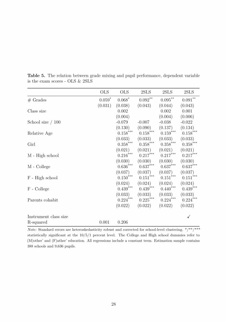
Table 5. The relation between grade mixing and pupil performance, dependent variableis the exam scores - OLS & 2SLS
OLS OLS 2SLS 2SLS 2SLS# Grades 0.059* 0.068* 0.092** 0.095** 0.091**
(0.031) (0.038) (0.043) (0.044) (0.043)Class size 0.002 0.002 0.001
(0.004) (0.004) (0.006)School size / 100 -0.079 -0.007 -0.038 -0.022
(0.130) (0.090) (0.137) (0.134)Relative Age 0.158*** 0.158*** 0.159*** 0.158***
(0.033) (0.033) (0.033) (0.033)Girl 0.358*** 0.358*** 0.358*** 0.358***
(0.021) (0.021) (0.021) (0.021)M - High school 0.216*** 0.217*** 0.217*** 0.217***
(0.030) (0.030) (0.030) (0.030)M - College 0.636*** 0.637*** 0.637*** 0.637***
(0.037) (0.037) (0.037) (0.037)F - High school 0.150*** 0.151*** 0.151*** 0.151***
(0.024) (0.024) (0.024) (0.024)F - College 0.439*** 0.439*** 0.440*** 0.439***
(0.033) (0.033) (0.033) (0.033)Parents cohabit 0.224*** 0.225*** 0.224*** 0.224***
(0.022) (0.022) (0.022) (0.022)
Instrument class size XR-squared 0.001 0.206Note: Standard errors are heteroskedasticity robust and corrected for school-level clustering. */**/***statistically significant at the 10/5/1 percent level. The College and High school dummies refer to(M)other’ and (F)ather’ education. All regressions include a constant term. Estimation sample contains388 schools and 9,636 pupils.
28
what is driving this result, Table 6 reports estimation results using equation (3). The top
panel of the table present estimates for exam scores and the second panel presents the
results for the teacher set and graded tests. For both outcomes we present OLS and 2SLS
estimates of the effects of g− and g+ , and also the effect of class size. To take away any
remaining concerns about omitted variables, such as endogenous sorting to schools we
also report estimation results from specifications that include school fixed effects.
In the first OLS specification the point estimate of the effect of exposure to the number
of lower grades (g− in equation 3) on exam scores is -0.11. This suggests that sharing
the classroom with a lower grade is detrimental for the exam scores, the point estimate
however lacks statistical significance at conventional levels. Pupils in classes where a
higher grade level is added score significantly higher on the exam. Adding school fixed
effects to the equation does not significantly change the estimates but comes at the cost
of a substantial loss in the precision of the estimates.
When we instrument both grade composition variables the point estimates increase.
For the number of lower grades we now obtain a point estimate of about -0.22 which is
close to being significant at the ten percent level. The point estimate for the number
of higher grades in the class room is 0.42 and significant at the 1 percent level. Recall
from Table 3 that if pupils are mixed, then they typically spend time with both lower and
higher grades. This explains the effects in Table 5: grade mixing is on average beneficial
because pupils benefit more from being with higher grades than they loose from being
with lower ones. The final column reports the 2SLS estimates from the specification
with school fixed effects. The effect for the number of lower grades drops but remains
negative even though it is no longer statistically significant. The effect for the number of
higher grader increases. We cannot reject equality of the 2SLS estimates with and without
fixed effects: when we bootstrap these estimates to perform a Wald test we obtain a test
statistic of 0.69 with a p-value of 0.708.
The second panel of Table 6 adds estimates for the teacher set and graded test scores.
These results confirm the conclusion based on the exam scores, namely that students
benefit from sharing the classroom with higher grades, and are harmed if the other
29
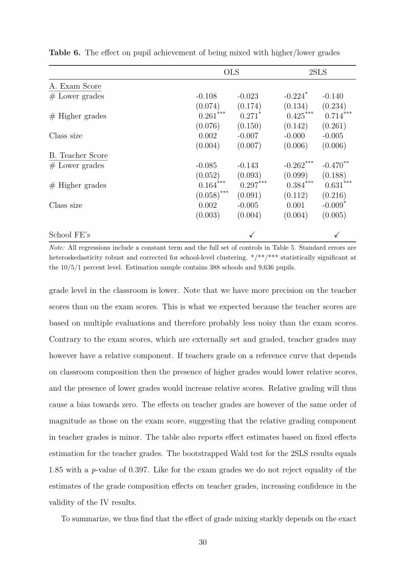
Table 6. The effect on pupil achievement of being mixed with higher/lower grades
OLS 2SLSA. Exam Score# Lower grades -0.108 -0.023 -0.224* -0.140
(0.074) (0.174) (0.134) (0.234)# Higher grades 0.261*** 0.271* 0.425*** 0.714***
(0.076) (0.150) (0.142) (0.261)Class size 0.002 -0.007 -0.000 -0.005
(0.004) (0.007) (0.006) (0.006)B. Teacher Score# Lower grades -0.085 -0.143 -0.262*** -0.470**
(0.052) (0.093) (0.099) (0.188)# Higher grades 0.164*** 0.297*** 0.384*** 0.631***
(0.058)*** (0.091) (0.112) (0.216)Class size 0.002 -0.005 0.001 -0.009*
(0.003) (0.004) (0.004) (0.005)
School FE’s X X
Note: All regressions include a constant term and the full set of controls in Table 5. Standard errors areheteroskedasticity robust and corrected for school-level clustering. */**/*** statistically significant atthe 10/5/1 percent level. Estimation sample contains 388 schools and 9,636 pupils.
grade level in the classroom is lower. Note that we have more precision on the teacher
scores than on the exam scores. This is what we expected because the teacher scores are
based on multiple evaluations and therefore probably less noisy than the exam scores.
Contrary to the exam scores, which are externally set and graded, teacher grades may
however have a relative component. If teachers grade on a reference curve that depends
on classroom composition then the presence of higher grades would lower relative scores,
and the presence of lower grades would increase relative scores. Relative grading will thus
cause a bias towards zero. The effects on teacher grades are however of the same order of
magnitude as those on the exam score, suggesting that the relative grading component
in teacher grades is minor. The table also reports effect estimates based on fixed effects
estimation for the teacher grades. The bootstrapped Wald test for the 2SLS results equals
1.85 with a p-value of 0.397. Like for the exam grades we do not reject equality of the
estimates of the grade composition effects on teacher grades, increasing confidence in the
validity of the IV results.
To summarize, we thus find that the effect of grade mixing starkly depends on the exact
30

grade composition of the classroom. In our study students benefit on average from grade
mixing. It is however important to point out that this not only depends on the positive
effects outweighing the negative ones, but also on the specific grade mixing sequences
students are exposed to. Interestingly, once we allow for this possibility we can reconcile
some of the apparently contradictory findings in the literature. A recent example is Sims
(2008), who finds a negative effect of the fraction of students in mixed-grade classrooms
on the (average) achievement of 2nd and 3rd graders. His instrument — the number
of classrooms that are saved by combining the current grade with lower grade pupils —
suggests that the complier group consists of schools who combine 2nd or 3rd graders with
pupils from lower grades to economize on the number of classrooms. In this case the
estimate will be the local average treatment effect of being mixed with lower grade pupils
which we expect to be negative. The positive effect of Thomas (2011) on the other hand
can be explained because it is the effect for first graders of sharing the classroom with
higher grade pupils, namely from 2nd grader.
5.2 Gender differences
Girls and boys experience different school outcomes. For example, not only do girls
outperform boys in reading in all countries in the PISA study, but in most countries this
gap is increasing (OECD, 2010). Boys score higher in mathematics, but there is no gender
gap in science performance. In nearly all OECD countries upper secondary graduation
rates for young women exceed those for young men (OECD, 2012). This relative good
performance of girls in compulsory schooling is also reflected by increased enrollment rates
of women in colleges with in some countries the gender gap even reversing in favor of
women (f.e. Goldin et al., 2006).
Although gender differences in educational performance are well documented, much
less is known about what underlies these differences. There is a growing literature
that documents systematic gender differences in risk preferences, social preferences, and
competitive preferences (Croson and Gneezy, 2009). On average, women are found to
be more risk averse, socially malleable and averse to competition. There is also a large
31

psychological literature that documents gender differences in social behavior (Eagly and
Wood, 1991). This suggests that peer groups may influence boys an girls differently.
There are studies that have compared peer effects for boys and girls in other contexts.
Lavy et al. (2009) find that in English secondary schools girls benefit more from better
peers than boys. Using data from Trinidad, Jackson (2010) also finds that the benefits of
attending schools with better performing pupils are larger for girls than for boys. Duflo
et al. (2008) also find larger effects of tracking on math performance for girls than for boys
in Kenya. Lavy and Schlosser (2011) on the other hand find that the classroom’s gender
composition affects boys and girls similarly in Israel, while Black et al. (2010) find positive
effects for girls and negative effects for boys in Norwegian lower secondary schools.
To investigate heterogeneity in the effect of a classroom’ grade composition, we therefore
perform our estimations separately by gender. The first two columns of Table 7 show
the effects of classroom grade composition first for girls and then for boys. We find in
the first column large and significant effects for girls’ exam scores. The positive effects
again dominate the negative ones. The point estimates go in the same direction for boys,
although the point estimate on the negative effect for lower grades is close to zero, and
the positive effect for higher grades is not significant. When we test for equality of the
effects across gender we can, however, not reject the null hypothesis that they are equal
(p=0.22).
The last two columns show the results for the teacher test scores. Here we have positive
and statistically significant effects of higher grades for both girls and boys. The estimates
are also of the same order of magnitude. We again find negative effects, this time for both
genders even though we lack precision for boys. We again do not reject equality of the
effects across gender (p=0.43).
One interesting aspect of the results for teacher test scores is their size relative to
those for the centralized exams. For girls the estimated effects are smaller, whereas for
boys they are larger. Although the average results above gave no indication that relative
grading mattered, the results for girls are consistent with this explanation. The results
for boys are however more difficult to reconcile with relative grading because there we see
32
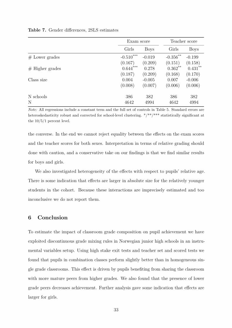
Table 7. Gender differences, 2SLS estimates
Exam score Teacher scoreGirls Boys Girls Boys
# Lower grades -0.510*** -0.019 -0.356** -0.199(0.167) (0.209) (0.151) (0.158)
# Higher grades 0.644*** 0.278 0.362** 0.431**
(0.187) (0.209) (0.168) (0.170)Class size 0.004 -0.005 0.007 -0.006
(0.008) (0.007) (0.006) (0.006)
N schools 386 382 386 382N 4642 4994 4642 4994Note: All regressions include a constant term and the full set of controls in Table 5. Standard errors areheteroskedasticity robust and corrected for school-level clustering. */**/*** statistically significant atthe 10/5/1 percent level.
the converse. In the end we cannot reject equality between the effects on the exam scores
and the teacher scores for both sexes. Interpretation in terms of relative grading should
done with caution, and a conservative take on our findings is that we find similar results
for boys and girls.
We also investigated heterogeneity of the effects with respect to pupils’ relative age.
There is some indication that effects are larger in absolute size for the relatively younger
students in the cohort. Because these interactions are imprecisely estimated and too
inconclusive we do not report them.
6 Conclusion
To estimate the impact of classroom grade composition on pupil achievement we have
exploited discontinuous grade mixing rules in Norwegian junior high schools in an instru-
mental variables setup. Using high stake exit tests and teacher set and scored tests we
found that pupils in combination classes perform slightly better than in homogeneous sin-
gle grade classrooms. This effect is driven by pupils benefiting from sharing the classroom
with more mature peers from higher grades. We also found that the presence of lower
grade peers decreases achievement. Further analysis gave some indication that effects are
larger for girls.
33
Our results contribute to two strands of work. The first literature to which we
contribute studies the nature and consequences of peer effects. A classroom becomes
more heterogeneous when two or more grades are mixed. This opens the scope for
direct negative or positive spillovers due to the presence of more or less able peers. Our
results are consistent with such externalities. The second, and main, contribution of our
paper concerns combination classes which, as we documented in the introduction, are an
important mode of classroom organization around the world. We know however little
about how time in such classes affects pupils’s learning outcomes. Our results show that
pupils can on average benefit from them, but we also find that this depends crucially on
how the classroom is balanced in terms of lower and higher grades. We take this also as
a cautionary tale. Pupils can be worse off if negative effects of lower grades cannot be
countered with positive effects channeled by the presence of higher grades.
References
Ammermueller, A. and Pischke, J.-S. (2009). Peer effects in european primary schools:
Evidence from the progress in international reading literacy study. Journal of Labor
Economics, 27(3):315–348.
Angrist, J. D. and Lang, K. (2004). Does school integration generate peer effects? evidence
from boston’s metco program. American Economic Review, 94(5):1613–1634.
Angrist, J. D. and Lavy, V. (1999). Using Maimonides’ Rule to Estimate The Effect of
Class Size on Scholastic Achievement. Quarterly journal of economics, 114(2):533–575.
Bedard, K. and Dhuey, E. (2006). The persistence of early childhood maturity: Interna-
tional evidence of long-run age effects. Quarterly Journal of Economics, 121(4):1437–
1472.
Black, S. E., Devereux, P. J., and Salvanes, K. G. (2010). Under pressure? the effect of
peers on outcomes of young adults. Working Paper No. 16004, NBER.
Boozer, M. A. and Cacciola, S. E. (2001). Inside the’black box’of project STAR: Estimation
34
of peer effects using experimental data. Working paper, Economic Growth Center, Yale
University.
Cahan, S. and Cohen, N. (1989). Age versus schooling effects on intelligence development.
Child Development, 60(5):1239–1249.
Croson, R. and Gneezy, U. (2009). Gender differences in preferences. Journal of Economic
Literature, 47(2):448–474.
Duflo, E., Dupas, P., and Kremer, M. (2008). Peer effects, teacher incentives, and the
impact of tracking: Evidence from a randomized evaluation in Kenya. Working Paper
No. 14475, NBER.
Eagly, A. and Wood, W. (1991). Explaining sex differences in social behavior: A meta-
analytic perspective. Personality and Social Psychology Bulletin, 17(3):306–315.
Fradette, A. and Lataille-Démoré, D. (2003). Les classes à niveaux multiples: point
mort ou tremplin pour l’innovation pédagogique. Revue des Sciences de l’Éducation,
29(3):589–607.
Fredriksson, P. and Öckert, B. (2005). Is early learning really more productive? the effect
of school starting age on school and labor market performance.
Goldin, C., Katz, L. F., and Kuziemko, I. (2006).
Hægeland, T., Raaum, O., and Salvanes, K. G. (2008). Pennies from heaven? using
exogeneous tax variation to identify effects of school resources on pupil achievements.
Discussion Paper 3561, Institute for the Study of Labor (IZA).
Heckman, J. J. and Smith, J. A. (1995). Assessing the case for social experiments. The
Journal of Economic Perspectives, 9(2):85–110.
Hoxby, C. M. (2000). Peer effects in the classroom: Learning from gender and race
variation. Working Paper No. 7867, NBER.
35
Jackson, C. (2010). Do students benefit from attending better schools?: Evidence from
rule-based student assignments in trinidad and tobago. The Economic Journal, 120(549).
Krueger, A. (1999). Experimental estimates of education production functions. The
Quarterly Journal of Economics, 114(2):497–532.
Lavy, V., Paserman, M. D., and Schlosser, A. (2008). Inside the black box of ability peer
effects: Evidence from variation in low achievers in the classroom. Working Paper No.
14415, NBER.
Lavy, V. and Schlosser, A. (2011). Mechanisms and impacts of gender peer effects at
school. American Economic Journal: Applied Economics, 3(2):1–33.
Lavy, V., Silva, O., and Weinhardt, F. (2009). The good, the bad and the average:
Evidence on the scale and nature of ability peer effects in schools. Working Paper No.
16500, NBER.
Leuven, E., Lindahl, M., Oosterbeek, H., and Webbink, H. D. (2010). Expanding schooling
opportunities for 4-year-olds. Economics of Education Review, 29:319–328.
Leuven, E., Oosterbeek, H., and Rønning, M. (2008). Quasi-experimental estimates of
the effect of class size on achievement in norway. Scandinavian Journal of Economics,
110(4):663–693.
Little, A. W. (2004). Learning and teaching in multigrade settings. Paper prepared for
the UNESCO 2005 EFA Monitoring Report.
Manski, C. F. (1993). Identification of endogenous social effects: The reflection problem.
The Review of Economic Studies, 60(3):531–542.
Mason, D. A. and Burns, R. B. (1997). Reassessing the effects of combination classes.
Educational Research and Evaluation.
McCrary, J. (2008). Manipulation of the running variable in the regression discontinuity
design: A density test. Journal of Econometrics, 142(2):698–714.
36
Mulryan-Kyne, C. (2005). The grouping practices of teachers in small two-teacher primary
schools in the Republic of Ireland. Journal of Research in Rural Education, 20(17):20–17.
OECD (2010). PISA 2009 Results: Learning Trends. Paris.
OECD (2012). Education At A Glance 2012. Paris.
Rothstein, J. (2010). Teacher quality in educational production: Tracking, decay, and
student achievement. Quarterly Journal of Economics, 125(1):175–214.
Sims, D. (2008). A strategic response to class size reduction: Combination classes
and student achievement in California. Journal of Policy Analysis and Management,
27(3):457–478.
Sojourner, A. (2008). Inference on peer effects with missing peer data: Evidence from
project STAR. Unpublished manuscript, Department of Economics, Northwestern
University.
Strøm, B. (2004). Student achievement and birthday effects. Unpublished manuscript,
Norwegian University of Science and Technology.
Thomas, J. L. (2011). Combination classes and educational achievement. Unpublished
working paper, Department of Economics, UC San Diego.
Urquiola, M. and Verhoogen, E. (2009). Class-size caps, sorting, and the regression-
discontinuity design. American Economic Review, 99(1):179–215.
Veenman, S. (1995). Cognitive and noncognitive effects of multigrade and multi-age
classes: A best-evidence synthesis. Review of Educational Research, 65(4):319–381.
37
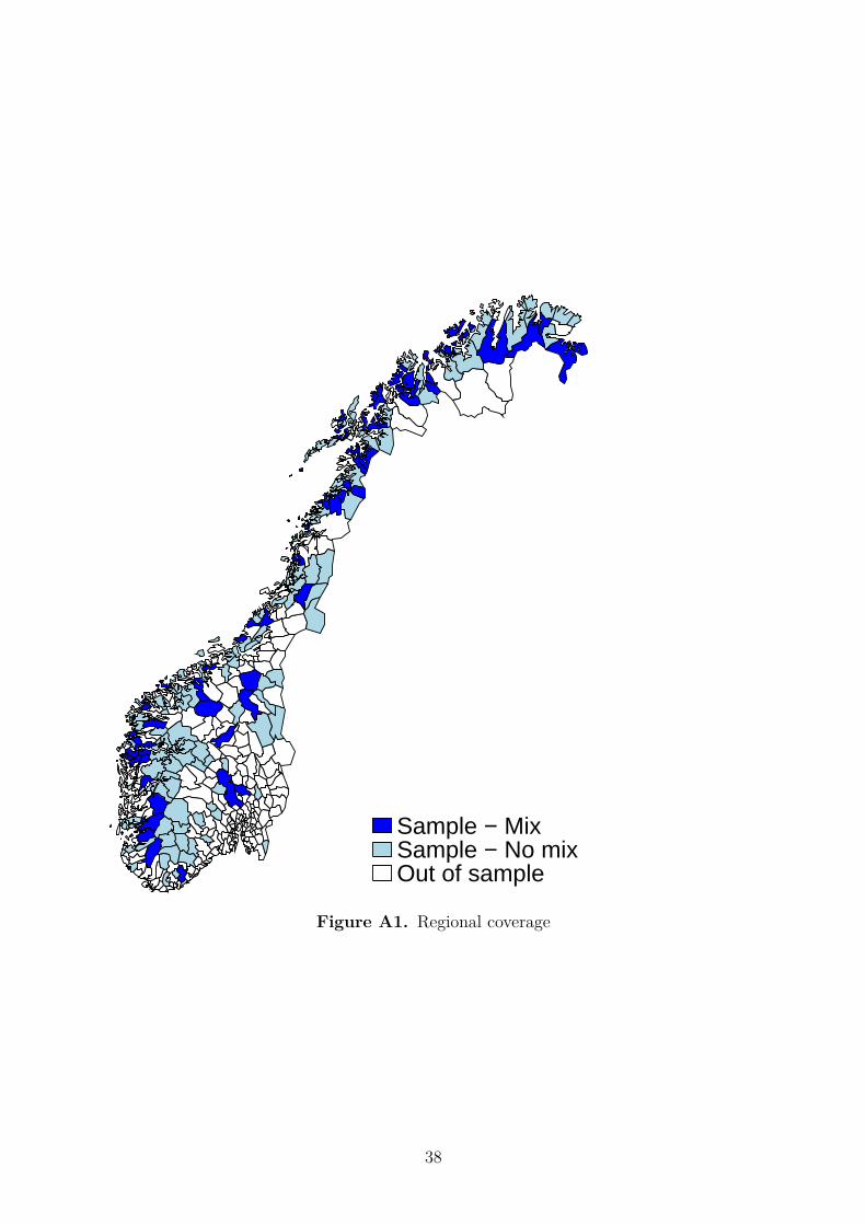
Sample − MixSample − No mixOut of sample
Figure A1. Regional coverage
38

From:Statistics Norway
Postal address:PO Box 8131 DeptNO-0033 Oslo
Offi ce address:Kongens gate 6, OsloOterveien 23, Kongsvinger
E-mail: [email protected]: www.ssb.noTelephone: + 47 62 88 50 00
ISSN 0809-733X
B Return to:Statistisk sentralbyråNO-2225 Kongsvinger
Desig
n: Siri B
oq
uist