Atmospheric CO2 increased from 280to 300 parts per million in 1880 to 335 to340 ppm in 1980 (1, 2), mainly due toburning of fossil fuels. Deforestation andchanges in biosphere growth may also

SCIENCE

Greenhouse Effect

The effective radiating temperature ofthe earth, Te, is determined by the needfor infrared emission from the planet tobalance absorbed solar radiation:

'rrR2(1 - A)So = 41TR2cT, (1)or

Te = [So(1 -A)/4or] " (2)where R is the radius of the earth, A thealbedo of the earth, S0 the flux of solarradiation, and a the Stefan-Boltzmannconstant. For A - 0.3 and So = 1367watts per square meter, this yieldsTe - 255 K.The mean surface temperature is

T-- 288 K. The excess, Ts - Te, is thegreenhouse effect of gases and clouds,which cause the mean radiating level tobe above the surface. An estimate of thegreenhouse warming is

The major difficulty in accepting thistheory has been the absence of observedwarming coincident with the historicCO2 increase. In fact, the temperature irthe Northern Hemisphere decreased by

Summary. The global temperature rose by 0.20C between the middle 1960's and1980, yielding a warming of 0.4°C in the past century. This temperature increase isconsistent with the calculated greenhouse effect due to measured increases ofatmospheric carbon dioxide. Variations of volcanic aerosols and possibly solarluminosity appear to be primary causes of observed fluctuations about the mean trendof increasing temperature. It is shown that the anthropogenic carbon dioxide warmingshould emerge from the noise level of natural climate variability by the end of thecentury, and there is a high probability of warming in the 1980's. Potential effects onclimate in the 21st century include the creation of drought-prone regions in NorthAmerica and central Asia as part of a shifting of climatic zones, erosion of the WestAntarctic ice sheet with a consequent worldwide rise in sea level, and opening of thefabled Northwest Passage.

have contributed, but their net effect isprobably limited in magnitude (2, 3). TheCO2 abundance is expected to reach 600ppm in the next century, even if growthof fossil fuel use is slow (4).Carbon dioxide absorbs in the atmo-

spheric "window" from 7 to 14 micro-meters which transmits thermal radiationemitted by the earth's surface and loweratmosphere. Increased atmospheric CO2tends to close this window and cause

outgoing radiation to emerge from high-er, colder levels, thus warming the sur-face and lower atmosphere by the so-

called greenhouse mechanism (5). Themost sophisticated models suggest a

mean warming of 2° to 3.5°C for doublingof the CO2 concentration from 300 to 600ppm (6-8).SCIENCE, VOL. 213, 28 AUGUST 1981

about 0.5°C between 1940 and 1970 (9), a

time of rapid CO2 buildup. In addition,recent claims that climate models over-

estimate the impact of radiative pertur-bations by an order of magnitude (10, 11)have raised the issue of whether thegreenhouse effect is well understood.We first describe the greenhouse

mechanism and use a simple model tocompare potential radiative perturba-tions of climate. We construct the trendof observed global temperature for thepast century and compare this with glob-al climate model computations, provid-ing a check on the ability of the model tosimulate known climate change. Finally,we compute the CO2 warming expectedin the coming century and discuss itspotential implications.

Ts7 Te + rH (3)where H is the flux-weighted mean alti-tude of the emission to space and r is themean temperature gradient (lapse rate)between the surface and H. The earth'stroposphere is sufficiently opaque in theinfrared that the purely radiative verticaltemperature gradient is convectively un-

stable, giving rise to atmospheric mo-

tions that contribute to vertical transportof heat and result in r 50 to 6°C perkilometer. The mean lapse rate is lessthan the dry adiabatic value because oflatent heat release by condensation as

moist air rises and cools and because theatmospheric motions that transport heatvertically include large-scale atmospher-ic dynamics as well as local convection.The value ofH is -5 km at midlatitudes(where r 6.5°C km-') and -6 km inthe global mean (r 5.5°C km-1).The surface temperature resulting

from flt greenhouse effect is analogousto thE1tfrof water in a leaky bucketwith cmnSWA inflow rate. If the holes inthe bucket are reduced slightly in size,the water depth and water pressure will

The authors are atmospheric physicists at theNASA Institute for Space Studies, Goddard SpaceFlight Center, New York 10025. D. Johnson contrib-uted to the carbon dioxide research as a participantin the Summer Institute on Planets and Climate atthe Goddard Institute for Space Studies and Colum-bia University.

0036-8075/81/0828-0957$01.00/0 Copyright 1981 AAAS

28 August 1981, Volume 213, Number 4511

Climate Impact of IncreasingAtmospheric Carbon Dioxide

J. Hansen, D. Johnson, A. Lacis, S. Lebedeff

P. Lee, D. Rind, G. Russell

957

on

July

5, 2

012

ww

w.s

cien

cem

ag.o

rgD

ownl

oade

d fr

om

increase until the flow rate out of theholes again equals the inflow rate. Anal-ogously, if the atmospheric infraredopacity increases, the temperature of thesurface and atmosphere will increase un-til the emission of radiation from theplanet again equals the absorbed solarenergy.The greenhouse theory can be tested

by examination of several planets, whichprovide an ensemble of experimentsover a wide range of conditions. Theatmospheric composition of Mars,Earth, and Venus lead to mean radiatinglevels of about 1, 6, and 70 km, and lapserates of F 50o, 5.50, and 7°C km-,respectively. Observed surface tempera-tures of these planets confirm the exis-tence and order of magnitude of thepredicted greenhouse effect (Eq. 3). Datanow being collected by spacecraft atVenus and Mars (12) will permit moreprecise analyses of radiative and dynam-ical mechanisms that affect greenhousewarming.

One-Dimensional Model

A one-dimensional radiative-convec-tive (1-D RC) model (5, 13), which com-putes temperature as a function of alti-tude, can simulate planetary tempera-tures more realistically than the zero-dimensional model of Eq. 1. Thesensitivity of surface temperature in 1-DRC models to changes in CO2 is similarto the sensitivity of mean surface tem-perature in global three-dimensionalmodels (6-8). This agreement does notvalidate the models; it only suggests thatone-dimensional models can simulate theeffect of certain basic mechanisms andfeedbacks. But the agreement does per-mit useful studies of global mean tem-perature change with a simple one-di-mensional model.The l-D RC model uses a time-march-

ing procedure to compute the verticaltemperature profile from the net radia-tive and convective energy fluxes:

T(h, t + At) =

T(h, t) +/dFr + dFc (4)

cpp dhi dh)

where cp is the heat capacity at constantpressure, p the density of air, h thealtitude, and dF/dh and dFIdh the netradiative and convective flux diver-gences. To compute dF/dh the radiativetransfer equation is integrated over allfrequencies, using the temperature pro-ifie of the previous time step and anassumed atmospheric composition. The

958

term dFI/dh is the energy transport need-ed to prevent the temperature gradientfrom exceeding a preassigned limit, usu-ally 6.5°C km-'. This limit parameterizeseffects of vertical mixing and large-scaledynamics.The radiative calculations are made by

a method that groups absorption coeffi-cients by strength for efficiency (14).Pressure- and temperature-dependentabsorption coefficients are from line-by-line calculations for H20, C02, 03, N20,and CH4 (15), including continuum H20absorption (16). Climatological cloudcover (50 percent) and aerosol properties(17) are used, with appropriate fractionsof low (0.3), middle (0.1), and high (0.1)clouds. Wavelength dependences ofcloud and aerosol properties are ob-tained from Mie scattering theory (14).Multiple scattering and overlap of gas-eous absorption bands are included. Ourcomputations include the weak CO2bands at 8 to 12 ,um, but the strong 15-,um CO2 band, which closes one side ofthe 7- to 20-Rm H20 window, causes- 90 percent of the CO2 warming.

Model Sensitivity

We examine the main processesknown to influence climate model sensi-tivity by inserting them individually intothe model, as summarized in Table 1.Model 1 has fixed absolute humidity, a

fixed lapse rate of 6.5°C km-l in theconvective region, fixed cloud altitude,and no snow/ice albedo feedback or veg-etation albedo feedback. The increase ofequilibrium surface temperature for dou-bled atmospheric CO2 is ATs- 1.2°C.This case is of special interest because itis the purely radiative-convective result,with no feedback effects.Model 2 has fixed relative humidity,

but is otherwise the same as model 1.The resulting AT, for doubled CO2 is

- 1.9°C. Thus the increasing water vaporwith higher temperature provides a feed-back factor of -1.6. Fixed relative hu-midity is clearly more realistic than fixedabsolute humidity, as indicated by physi-cal arguments (13) and three-dimensionalmodel results (7, 8). Therefore, we usefixed relative humidity in the succeedingexperiments and compare models 3 to 6with model 2.Model 3 has a moist adiabatic lapse

rate in the convective region rather thana fixed lapse rate. This causes the equi-librium surface temperature to be lesssensitive to radiative perturbations, andAT, - 1.4°C for doubled CO2. The rea-son is that the lapse rate decreases as

moisture is added to the air, reducing thetemperature difference between the topof the convective region and the ground(rH in Eq. 3).The general circulation of the earth's

atmosphere is driven by solar heating ofthe tropical ocean, and resulting evapo-ration and vertical transport of energy.The lapse rate is nearly moist adiabaticat low latitudes and should remain soafter a climate perturbation. Thus use ofa moist adiabatic lapse rate is appropri-ate for the tropics. But more stable lapserates at high latitudes make the surfacetemperature much more sensitive to per-turbations of surface heating (7, 8), andhence model 3 would underestimate thesensitivity there. -

Model 4 has the clouds at fixed tem-perature levels, and thus they move to ahigher altitude as the temperature in-creases (18). This yields AT, - 2.8°C fordoubled C02, compared to 1.9°C forfixed cloud altitude. The sensitivity in-creases because the outgoing thermalradiation from cloudy regions is definedby the fixed cloud temperature, requiringgreater adjustment by the ground andlower atmosphere for outgoing radiationto balance absorbed solar radiation.

Study of Venus suggests that someclouds occur at a fixed temperature. TheVenus cloud tops, which are the primaryradiator to space, are at H - 70 km,where T - Te. Analysis of the processesthat determine the location of theseclouds and the variety of clouds in thebelts, zones, and polar regions on Jupitershould be informative. Available evi-dence suggests that the level of someterrestrial clouds depends on tempera-ture while others occur at a fixed alti-tude. For example, tropical cirrus cloudsmoved to a higher altitude in the experi-ment of Hansen et al. (8) with doubledC02, but low clouds did not noticeablychange altitude.Models 5 and 6 illustrate snow/ice and

vegetation albedo feedbacks (19, 20).Both feedbacks increase model sensitiv-ity, since increased temperature de-creases ground albedo and increases ab-sorption of solar radiation.Snow, sea ice, and land ice (ice sheets

and glaciers) are all included in snow/icealbedo feedback. Snow and sea ice re-spond rapidly to temperature change,while continental ice sheets require thou-sands of years to respond. Thus a partialsnow/ice albedo feedback is appropriatefor time scales of 10 to 100 years. Thevegetation albedo feedback was obtainedby comparing today's global vegetationpatterns with reconstruction of the Wis-consin ice age (20). Uncertainties in the

SCIENCE, VOL. 213

on

July

5, 2

012

ww

w.s

cien

cem

ag.o

rgD

ownl

oade

d fr

om

reconstruction, the time scale of vegeta-tion response, and man's potential im-pact on vegetation prevent reliable as-sessment of this feedback, but its esti-mated magnitude emphasizes the need tomonitor global vegetation and surfacealbedo.Model 4 has our estimate of appropri-

ate model sensitivity. The fixed 6.5°Ckm-' lapse rate is a compromise be-tween expected lower sensitivity at lowlatitudes and greater sensitivity at highlatitudes. Both cloud temperature andsnow/ice albedo feedback should bepartly effective, so for simplicity one isincluded.The sensitivity of the climate model

we use is thus ATs - 2.8°C for doubledC02, similar to the sensitivity of three-dimensional climate models (6-8). Theestimated uncertainty is a factor of 2.This sensitivity (i) refers to perturbationsabout today's climate and (ii) does notinclude feedback mechanisms effectiveonly on long time scales, such as changesof ice sheets or ocean chemistry.

Model Time Dependence

The time dependence of the earth'ssurface temperature depends on the heatcapacity of the climate system. Heatcapacity of land areas can be neglected,since ground is a good insulator. Howev-er, the upper 100 m of the ocean israpidly mixed, so its heat capacity mustbe accounted for. The ocean beneath themixed layer may also affect surface tem-perature, if the thermal response time ofthe mixed layer is comparable to the timefor exchange of heat with deeper layers.The great heat capacity of the ocean

and ready exchange of continental andmarine air imply that the global climateresponse to perturbations is determinedby the response of the ocean areas.However, this response is affected byhorizontal atmospheric heat fluxes fromand to the continents. Ready exchangeof energy between the ocean surface andatmosphere "fixes" the air temperature,and the ocean in effect removes from theatmosphere any net heat obtained fromthe continents. Thus the horizontal fluxdue to a climate perturbation's heating(or cooling) of the continents adds to thevertical heat flux into (or out of) theocean surface. The net flux into theocean surface is therefore larger than itwould be for a 100 percent ocean-cov-ered planet by the ratio of global area toocean area, totaling -5.7 W m-2 fordoubled CO2 rather than -4W m2. In aclimate model that employs only a

28 AUGUST 1981

Table 1. Equilibrium surface temperature increase due to doubled CO2 (from 300 to 600 ppm) inl-D RC models. Model I has no feedbacks affecting the atmosphere's radiative properties.Feedback factorf specifies the effect of each added process on model sensitivity to doubledC02; F is the equilibrium thermal flux into the ground if T. is held fixed (infinite heat capacity)when CO2 is doubled. Abbreviations: FRH, fixed relative humidity; FAH, fixed absolutehumidity; 6.5LR, 6.5°C km-' limiting lapse rate; MALR, moist adiabatic limiting lapse rate;FCA, fixed cloud altitude, FCT, fixed cloud temperature; SAF, snow/ice albedo feedback; andVAF, vegetation albedo feedback. Models 5 and 6 are based onfvalues from Wang and Stone(19) and Cess (20), respectively, and AT, of model 2.

AT, FModel Description (OC) f (W m-2)

1 FAH, 6.5LR, FCA 1.22 1 4.02 FRH, 6.5LR, FCA 1.94 1.6 3.93 Same as 2, except MALR replaces 6.5LR 1.37 0.7 4.04 Same as 2, except FCT replaces FCA 2.78 1.4 3.95 Same as 2, except SAF included 2.5-2.8 1.3-1.46 Same as 2, except VAF included -3.5 -1.8

mixed-layer ocean, it is equivalent to usethe flux -4 W m-2 with the area-weight-ed mean land-ocean heat capacity.The thermal response time of the

ocean mixed layer would be -3 years ifit were not for feedback effects in theclimate system. For example, assumethat the solar flux absorbed by a planetchanges suddenly from Fo orT04 toF1 = Fo + AF ocT,4, with AF << Fo.The rate of change of heat in the climatesystem is

d(cT)ldt = aT14 - aT4 (5)

where c is heat capacity per unit area.Since T1 - To << To, the solution is

T - T, = (To - TI)e-t/tthr (6)where

tthr = c/4aT,3 (7)

Thus the planet approaches a new equi-librium temperature exponentially withe-folding time tthr. If the heat capacity isprovided by 70 m of water (100 m forocean areas) and the effective tempera-ture is 255 K, tthr is 2.8 years.

This estimate does not account forclimate feedback effects, which can beanalyzed with the 1-D RC model. Table 1shows that the initial rate of heat storagein the ocean is independent offeedbacks.Thus the time needed to reach equilibri-um for model 4 is larger by the factor-2.8°C/1.2°C than for model 1, whichexcludes feedbacks. The e-folding timefor adjustment of mixed-layer tempera-ture is therefore -6 years for our bestestimate of model sensitivity to doubledCO2. This increase in thermal responsetime is readily understandable, becausefeedbacks come into play only graduallyafter some warming occurs.

It would take --50 years to warm upthe thermocline and mixed layer if theywere rapidly mixed, or 250 years for theentire ocean. Turnover of the deep

ocean, driven by formation of cold bot-tom water in the North Atlantic andAntarctic oceans with slow upwelling atlow latitudes, is thought to require 500 to1000 years (21), suggesting that the deepocean does not greatly influence surfacetemperature sensitivity. However, theremay be sufficient heat exchange betweenthe mixed layer and thermocline to delayfull impact of a climate perturbation by afew decades (6, 22, 23). The primarymechanism of exchange is nearly hori-zontal movement of water along surfacesof constant density (21).Delay of CO2 warming by the ocean

can be illustrated with a "box diffusion"model (24), in which heat is stirred in-stantly through the mixed layer and dif-fused into the thermocline with diffusioncoefficient k. Observed oceanic penetra-tion by inert chemical tracers suggeststhat k is of order 1 square centimeter persecond (2, 3, 24).The warming calculated with the one-

dimensional model for the CO2 increasefrom 1880 to 1980 (25) is 0.5°C if oceanheat capacity is neglected (Fig. 1). Theheat capacity of just the mixed layerreduces this to O.4°C, a direct effect ofthe mixed layer's 6-year thermal re-sponse time. Diffusion into the thermo-cline further reduces the warming to0.25°C for k = 1 cm2 sec-', an indirecteffect of the mixed layer's 6-year e-folding time, which permits substantialexchange with the thermocline.The mixed-layer model and thermo-

cline model bracket the likely CO2warming. The thermocline model is pref-erable for small climate perturbationsthat do not affect ocean mixing. Howev-er, one effect of warming the ocean sur-face will be increased vertical stability,which could reduce ocean warming andmake the surface temperature responsemore like that of the mixed-layer case.Lack of knowledge of ocean processes

959

on

July

5, 2

012

ww

w.s

cien

cem

ag.o

rgD

ownl

oade

d fr

om

1.0 -

0.8

0.6

00LI- 0.4

0.2

0 -1880 1900 1920 1940

Date

primarily introduces uncertainties aboutthe time dependence of the global CO2warming. The full impact of the warmingmay be delayed several decades, butsince man-made increases in atmospher-ic CO2 are expected to persist for centu-ries (1, 2, 6), the warming will eventuallyoccur.

Radiative Climate Perturbations

Identification of the CO2 warming inobserved climate depends on the magni-tude of climate variability due to otherfactors. Most suspected causes of globalclimate change are radiative perturba-tions, which can be compared to identifythose capable of counteracting or rein-forcing the CO2 warming.

1960 1980 2000

-1.3 -1.4

C02 Strat, Tropo. Low High(300 ppm - aerosols aerosols clouds clouds

600 ppm) H2804 Soot (+2% of (+2% of

(|&ru+0.2) (&rT+0.02) globe) globe)

Solar Tropo. Land Middle Iluminosity aerosols albedo clouds (0.2

CH4(1.6 ppm

-3.2 ppm)

N20 CCI2F2 &

28 ppm CCI3F

(+1%) H2804 (+0.05) (+2% of -0.56 ppm)(0-2 ppb(Aru+0. 1) globe) each)

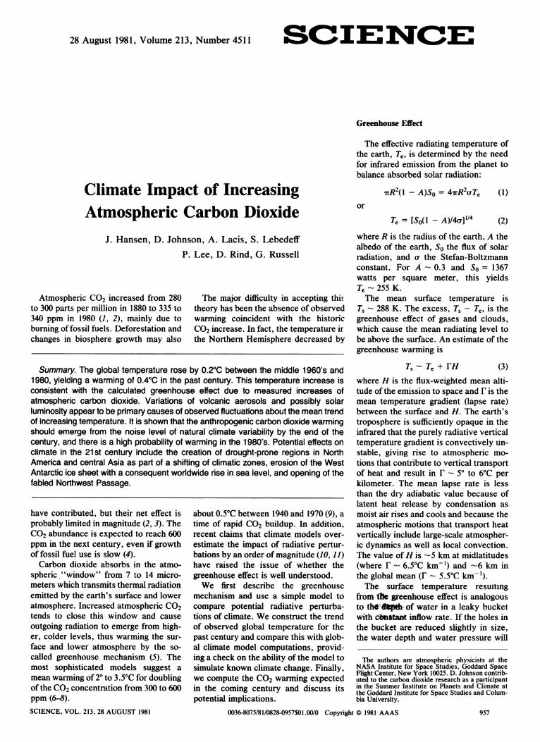
Fig. 2. Surface temperature effect of various global radiative perturbations, based on the l-DRC model 4 (Table 1). Aerosols have the physical properties specified by (17). Dependence ofAT on aerosol size, composition, altitude, and optical thickness is illustrated by (26). The AT forstratospheric aerosols is representative of a very large volcanic eruption.

960

Fig. 1. Dependence ofCO2 warming onocean heat capacity.Heat is rapidly mixedin the upper 100 m ofthe ocean and dif-fused to 1000 m withdiffusion coefficient k.The CO2 abundance,from (25), is 293 ppmin 1880, 335 ppm in1980, and 373 ppm in2000. Climate modelequilibrium sensitiv-ity is 2.8°C for dou-bled CO2.

A 1 percent increase of solar luminos-ity would warm the earth 1.6°C at equi-librium (Fig. 2) on the basis of model 4,which we employ for all radiative pertur-bations to provide a uniform compari-son. Since the effect is linear for smallchanges of solar luminosity, a change of0.3 percent would modify the equilibri-um global mean temperature by 0.5°C,which is as large as the equilibriumwarming for the cumulative increase ofatmospheric CO2 from 1880 to 1980. So-lar luminosity variations of a few tenthsof 1 percent could not be reliably mea-sured with the techniques available dur-ing the past century, and thus are apossible cause of part of the climatevariability in that period.Atmospheric aerosol effects depend

on aerosol composition, size, altitude,

and global distribution (26). Based onmodel calculations, stratospheric aero-sols that persist for 1 to 3 years afterlarge volcanic eruptions can cause sub-stantial cooling of surface air (Fig. 2).The cooling depends on the assumptionthat the particles do not exceed a fewtenths of a micrometer in size, so they donot cause greenhouse warming by block-ing terrestrial radiation, but this condi-tion is probably ensured by rapid gravita-tional settling of larger particles. Tempo-ral variability of stratospheric aerosolsdue to volcanic eruptions appears tohave been responsible for a large part ofthe observed climate change during thepast century (27-30), as shown below.The impact of tropospheric aerosols

on climate is uncertain in sense andmagnitude due to their range of composi-tion, including absorbing material suchas carbon and high-albedo material suchas sulfuric acid, and their heterogeneousspatial distribution. Although man-madetropospheric aerosols are obvious neartheir source, aerosol opacity does notappear to have increased much in remoteregions (31). Since the climate impact ofanthropogenic aerosols is also reducedby the opposing effects of absorbing andhigh-albedo materials, it is possible thatthey have not had a primary effect onglobal temperature. However, globalmonitoring of aerosol properties is need-ed for conclusive analysis.Ground albedo alterations associated

with changing patterns of vegetationcoverage have been suggested as a causeof global climate variations on timescales of decades to centuries (32). Aglobal surface albedo change of 0.015,equivalent to a change of 0.05 over landareas, would affect global temperatureby 1.3°C. Since this is a 25 percentchange in mean continental ground albe-do, it seems unlikely that ground albedovariations have been the primary causeof recent global temperature trends.However, global monitoring of groundalbedo is needed to permit definitiveassessment of its role in climate variabili-ty.High and low clouds have opposite

effects on surface temperature (Fig. 2),high clouds having a greenhouse effectwhile low clouds cool the surface (14,33). However, the nature and causes ofvariability of cloud cover, optical thick-ness, and altitude distribution are notwell known, nor is it known how tomodel reliably cloud feedbacks that mayoccur in response to climate perturba-tions. Progress may be made after accu-rate cloud climatology is obtained fromglobal observations, including seasonaland interannual cloud variations. In the

SCIENCE, VOL. 213

4

3

00

_- 24

0

Potential radiative perturbations of climate

Warming 0 Cooling

-1.9

on

July

5, 2

012

ww

w.s

cien

cem

ag.o

rgD

ownl

oade

d fr

om

meantime, some limits are implicitlyplaced on global cloud feedback by em-pirical tests of the climate system's sen-sitivity to radiative perturbations, as dis-cussed below.Trace gases that absorb in the infrared

can warm the earth if their abundanceincreases (5, 34). The abundance ofchlorofluorocarbons (Freons) increasedfrom a negligible amount a few decadesago to 0.3 part per billion for CC12F2 and0.2 ppb for CC13F (35), with an equilibri-um greenhouse warming of - 0.06°C.Recent measurement of a 0.2 percent peryear increase of N20 suggests a cumula-tive increase to date of 17 ppb (36), withan equilibrium warming of - 0.03°C.Tentative indications of a 2 percent peryear increase in CH4 imply an equilibri-um warming < 0.1°(C for the CH4 in-crease to date (37). No major trend of 03abundance has been observed, althoughit has been argued that continued in-crease of Freons will reduce 03 amounts(38). The net impact of measured tracegases has thus been an equilibriumwarming of 0.1°C or slightly larger. Thisdoes not greatly alter analyses of tem-perature change over the past century,but trace gases will significantly enhancefuture greenhouse warming if recentgrowth rates are maintained.We conclude that study of global cli-

mate change on time scales of decadesand centuries must consider variabilityof stratospheric aerosols and solar lumi-nosity, in addition to CO2 and tracegases. Tropospheric aerosols and groundalbedo are potentially significant, butrequire better observations. Cloud vari-ability will continue to cause uncertaintyuntil accurate monitoring of global cloudproperties provides a basis for realisticmodeling of cloud feedback effects; how-ever, global feedback is implicitlychecked by comparison of climate modelsensitivity to empirical climate varia-tions, as done below.

Observed Temperature Trends

Data archives (39) contain surface airtemperatures of several hundred stationsfor the last century. Problems in obtain-ing a global temperature history are dueto the uneven station distribution (40),with the Southern Hemisphere andocean areas poorly represented, and thesmaller number of stations for earliertimes.

dynamical transports (41), but largeenough that most boxes contained one ormore stations. The results shown wereobtained with 40 equal-area boxes ineach hemisphere, but the conclusionsare not sensitive to the exact spacing.Temperature trends for stations within abox were combined successively:

T,n(t) (n* - l)T1,n + Tn - Tn + TI,n

(8)to obtain a single trend for each box,where the bar indicates a mean for theyears in which there are records for bothTn and the cumulative T1,n and n*(t) isthe number of stations in Tj,m(t). Trendsfor boxes in a latitude zone were com-bined with each box weighted equally,and the global trend was obtained byarea-weighting the trends for all latitudezones. A meaningful result begins in the1880's, since thereafter continuous rec-ords exist for at least two widely separat-ed longitudes in seven of the eight lati-tude zones (continuous Antarctic tem-peratures begin in the 1950's). Resultsare least reliable for 1880 to 1900; by1900, continuous records exist for morethan half of the 80 boxes.The temperature trends in Fig. 3 are

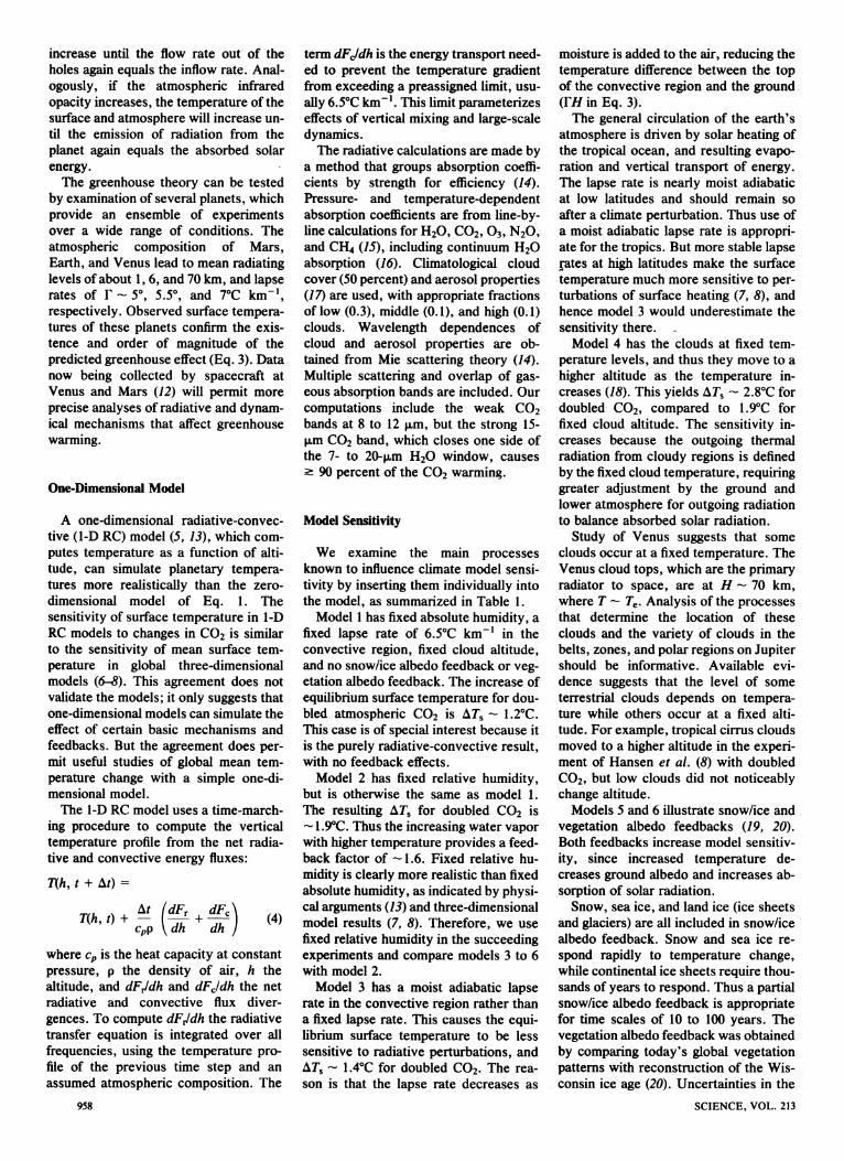
smoothed with a 5-year running mean tomake the trends readily visible. Part ofthe noise in the unsmoothed data resultsfrom unpredictable weather fluctuations,which affect even 1-year means (42).

Obseri

0.4

0.2

0

o -0.2-

-0.4 f

Fig. 3. Observed surface airtemperature trends for threelatitude bands and the entireglobe. Temperature scales forlow latitudes and global meanare on the right.

0.2

-0.2

We combined these temperature rec-ords with a method designed to extractmean temperature trends. The globe wasdivided by grids with a spacing not largerthan the correlation distance for primary28 AUGUST 1981

None of our conclusions depends on thenature of the smoothing.Northern latitudes warmed - 0.8UC

between the 1880's and 1940, thencooled - 0.5C between 1940 and 1970,m agreement with other analyses (9, 43).Low latitudes warmed - 0.3°C between1880 and 1930, with little change thereaf-ter. Southern latitudes warmed - 0.4°Cin the past century; results agree with aprior analysis for the late 1950's to mid-dle 1970's (44). The global mean tem-perature increased - 0.5°C between1885 and 1940, with slight cooling there-after.A remarkable conclusion from Fig. 3 is

that the global temperature is almost ashigh today as it was in 1940. The com-mon misconception that the world iscooling is based on Northern Hemi-sphere experience to 1970.Another conclusion is that global sur-

face air temperature rose - 0.4OC in thepast century, roughly consistent withcalculated CO2 warming. The time his-tory of the warming obviously does notfollow the course of the CO2 increase(Fig. 1), indicating that other factorsmiust affect global mean temperature.

Model Verification

Natural radiative perturbations of theearth's climate, such as those due toaerosols produced by large volcanic

ved temperature (5-year running mean)

0.2

owlatituides 0

-0.2

0outhern latitudes

zX~(3.608-900S)0..JX J\\ Al 0.2

Date

961

on

July

5, 2

012

ww

w.s

cien

cem

ag.o

rgD

ownl

oade

d fr

om

AS=O.1 A Ft* -2.4 Net-+2.5 AS*0.1

t II1 Atmos.

-0.3 + Surface

Ts = 287.5

(a) Imrmediate response

AFtu-3.8 Net*+3.9

t t+0.4 -0.8 -30 Atmos.

-0.3 -3.1 8 + 1. Surface

;0 .73 ,,7g, 7i .2Ts = 287.5

(b) A few months later

AS-0.l AF' -0.1 NetO0

t t+1.9 -1.4 +1.5 Atmos.--U-\--- - -1-T- E

-1.8 0 +171 Surface1+I6i6 17.Ts = 290.3

(c) Many years later

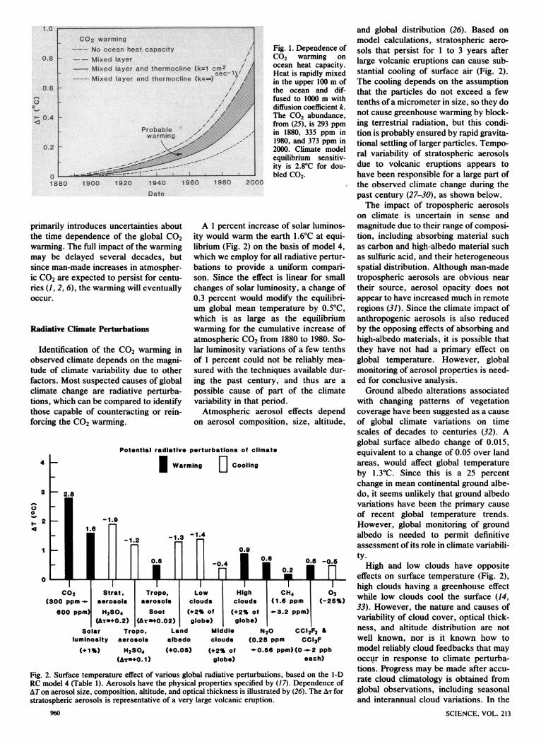
Fig. 4. Change of fluxes (watts per square meter) in the 1-D RC model when atmospheric CO2 is doubled (from 300 to 600 ppm). Symbols: AS,change in solar radiation absorbed by the atmosphere and surface; AF t , change in outward thermal radiation at top of the atmosphere. The wavyline represents convective flux; other fluxes are radiative.

eruptions, permit a valuable test of tnod-el sensitivity. Previous study of the best-documented large volcanic eruption,Mount Agung in 1963, showed that tropi-cal tropospheric and stratospheric tem-perature changes computed with a one-

dimensional climate model were of thesame sign and order of magnitude as

observed changes (45). It was assumedthat horizontal heat exchange with high-er latitudes was not altered by the radia-tive perturbation.We reexamined the Mount Agung case

for comparison with the present globaltemperature record, using our modelwith sensitivity - 2.8°C. The model,with a maximum global mean aerosolincrease in the optical depth AT = 0.12(45), yields a maximum global cooling of0.2°C when only the mixed-layer heatcapacity is included and 0.1C when heatexchange with the deeper ocean is in-

cluded with k = 1 cm2 sec-1. Observa-tions suggest a cooling of this magnitudewith the expected time lag of 1 to 2years. Noise or unexplained variabilityin the observations prevents more defini-tive conclusions, but similar cooling isindicated by statistical studies of tem-perature trends following other large vol-canic eruptions (46).A primary lesson from the Mount

Agung test is the damping of temperaturechange by the mixed layer's heat capaci-ty, without which the cooling wouldhave exceeded 1.1C (Fig. 2). The effectcan be understood from the time con-

stant of the perturbation and thermalresponse time of the mixed layer:AT {1 - exp[(- 1 year)/(6 years)]} x

1.1°C 0.17C, for the case k = 0. Thislarge reduction of the clitnate responseoccurs for a perturbation that (unlikeC02) is present for a time shorter thanthe thermal response time of the ocean

surface.Phenomena that alter the regional radi-

ation balance provide another modeltest. Idso (11) found a consistent "em-pirical response function" for severalsuch phenomena, which was 0.17C per

962

watt per square meter in midcontinentand was half as large on the coast. Thisresponse must depend on the rate ofmixing of marine and continental air,since the phenomena occur on timescales less than the thermal relaxationtime of the ocean surface. Thus, as onetest of horizontal atmospheric trans-ports, we read from our three-dimen-sional climate model (8) the quantities(solar insolation and temperature) thatform Idso's empirical response functionfor seasonal change of insolation. Re-sults ranged from 0.2°C W' m2 in mid-continent, and about half that on thecoast, to a value an order of magnitudesmaller over the ocean, in agreementwith the empirical response (11).To relate these empirical tests to the

CO2 greenhouse effect, we illustrate theflux changes in the I-D RC model whenCO2 is doubled. For simplicity we con-sider an instantaneous doubling of C02,and hence the time dependence of theresponse does not represent the transientresponse to a steady change in CO2. Theimmediate response to the doubling in-cludes (Fig. 4a): (i) reduced emission tospace (- 2.4W m-2), because added CO2absorption raises the mean altitude ofemission to a higher, colder level; (ii)increased flux from atmosphere toground (+ 1.1 W m2); and (iii) increasedstratospheric cooling but decreased tro-pospheric cooling. The radiative warm-ing of the troposphere decreases theconvective" flux (latent. and sensible

heat) from the ground by 3.5 W m72 as aconsequence of the requirement to con-serve energy. There is a small increase inabsorption of near-infrared radiation, theatmosphere gaining energy (+ 0.4 Wmf2) and the ground losing energy (- 0.3W m72). The net effect is thus an energygain for the planet (+ 2.5 W m-2) withheating of the ground (+ 4.3 W m-2) andcooling of the (upper) atmosphere (- 1.8W m72). These flux changes are indepen-dent offeedbacks and are not sensitive tothe critical lapse rate.A few months after the CO2 doubling

(Fig. 4b) the stratospheric temperaturehas cooled by - 5°C. Neither the oceannor the troposphere, which is convec-tively coupled to the surface, have re-sponded yet. The planet radiates 3.8 Wm72 less energy to space than in thecomparison case with 300 ppm CO2,because of the cooler stratosphere andgreater altitude of emission from thetroposphere. The energy gained by theearth at this time is being used to warmthe ocean.

Years later (Fig. 4c) the surface tem-perature has increased 2.8C. Almosthalf the increase (1.2°C) is the direct CO2greenhouse effect. The remainder is dueto feedbacks, of which 1.0°C is the well-established H20 greenhouse effect.The greenhouse process represented

in Fig. 4 is simply the "leaky bucket"phenomenon. The increased infraredopacity causes an immediate decrease ofthermal radiation from the planet, thusforcing the temperature to rise until ener-gy balance is restored. Temporal varia-tions of the fluxes and temperatures aredue to the response times of the atmo-sphere and surface.

Surface warming of - 3°C for doubledCO2 is the status after energy balancehas been restored. This contrasts withthe Agung case and the cases consideredby Idso (11), which are all nonequilibri-um situations.The test of the greenhouse theory pro-

vided by the extremes of equilibriumclimates on the planets and short-termradiative perturbations is reassuring, butinadequate. A crucial intermediate test isclimate change on time scales from a fewyears to a century.

Model versus Observations for the

Past Century

Simulations of global temperaturechange should begin with the knownforcings: variations of CO2 and volcanicaerosols. Solar luminosity variations,which constitute another likely mecha-

SCIENCE, VOL. 213

on

July

5, 2

012

ww

w.s

cien

cem

ag.o

rgD

ownl

oade

d fr

om

nism, are unknown, but there arehypotheses consistent with observation-al constraints that variations not exceeda few tenths of 1 percent.We developed an empirical equation

that fits the heat flux into the earth'ssurface calculated with the l-D RC cli-mate model (model 4):

F(t) = 0.018Ap/(l + 0.0022Ap)06-17AT - 1.5(AT)2 + 220AS/5O-1.5AT + 0.033 (Al)2 - 1.04 X

10ApAT + 0.29ATAT (9)

where F(t) is in watts per square meter, pis the amount of CO2 in parts per millionabove an "equilibrium" value (293ppm), AS is the difference between solarluminosity and an equilibrium value So,AT iS the optical depth of stratosphericaerosols above a background amount,and AT is the difference between currentsurface temperature and the equilibriumvalue for Ap = AS = AT = 0. Equation9 fits the one-dimensional model resultsto better than 1 percent for 0 s Ap< 1200 ppm, 0.98 c AS/SO c 1.02, andAT s 0.5. For the mixed-layer oceanmodel T,(t) follows from dTI/dt = F(t)lco, where co is the heat capacity of theocean mixed layer per unit area. If thetrue mixed-layer depth is used to obtainco, F(t) must be multiplied by 1/0.7, theratio of global area to ocean area. Diffu-sion of heat into the deeper ocean canthen also be included by means of thediffusion equation with T. as its upperboundary condition.The CO2 abundance increased from

293 ppm in 1880 to 335 ppm in 1980 (25),based on recent accurate observations,earlier less accurate observations, andcarbon cycle modeling. The error for1880 probably does not exceed 10 ppm(1, 2).

Volcanic aerosol radiative forcing canbe obtained from Lamb's (27) dust veilindex (DVI), which is based mainly onatmospheric transmission measurementsafter 1880. We convert DVI to opticaldepth by taking Mount Agung (DVI =800) to have the maximum AT = 0.12.The aerosol optical depth histories ofMitchell (47) and Pollack et al. (29), thelatter based solely on transmission mea-surements, are similar to Lamb's. Weuse aerosol microphysical propertiesfrom (45). The error in volcanic aerosolradiative forcing probably does not ex-ceed a factor of 2.

Solar variability is highly conjectural,so we first study CO2 and volcanic aero-sol forcings and then add solar varia-tions. We examine the hypothesis ofHoyt (48) that the ratio, r, of umbra topenumbra areas in sunspots is pro-28 AUGUST 1981

portional to solar luminosity: AS/So = fir - ro). Hoyt's rationale is thatthe penumbra, with a weaker magneticfield than the umbra, is destroyed morereadily by an increase of convective fluxfrom below. We take f = 0.03, whichimplies a peak-to-peak amplitude of

- 0.4 percent for AS/S0 in the past cen-tury, or an amplitude of - 0.2 percentfor the mean trend line. Taking So as themean for 1880 to 1976 yields ro= 0.2.The resulting AS/S0 has no observationalcorroboration, but serves as an exampleof solar variability of a plausible magni-tude.

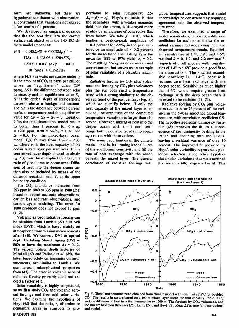
Radiative forcing by CO2 plus volca-noes and forcing by CO2 plus volcanoesplus the sun both yield a temperaturetrend with a strong similarity to the ob-served trend of the past century (Fig. 5),which we quantify below. If only theheat capacity of the mixed layer is in-cluded, the amplitude of the computedtemperature variations is larger than ob-served. However, mixing of heat into thedeeper ocean with k = 1 cm2 sec-1brings both calculated trends into roughagreement with observations.The main uncertainties in the climate

model-that is, its "tuning knobs"-are(i) the equilibrium sensitivity and (ii) therate of heat exchange with the oceanbeneath the mixed layer. The generalcorrelation of radiative forcings with

Ocean model: mixed layer only

0.2

0

-0.2

0

0

00

-0.2

-0.4

-0.6 I1 880 1920 1960

global temperatures suggests that modeluncertainties be constrained by requiringagreement with the observed tempera-ture trend.

Therefore, we examined a range ofmodel sensitivities, choosing a diffusioncoefficient for each to minimize the re-sidual yariance between computed andobserved temperature trends. Equilibri-um sensitivities of 1.4°, 2.80, and 5.6°Crequired k = 0, 1.2, and 2.2 cm2 sec-',respectively. All models with sensitiv-ities of 1.4° to 5.6°C provide a good fit tothe observations. The smallest accept-able sensitivity is - 1.4°C, because itrequires zero heat exchange with thedeeper ocean. Sensitivities much higherthan 5.60C would require greater heatexchange with the deep ocean than isbelieved to be realistic (21, 22).

Radiative forcing by CO2 plus volca-noes accounts for 75 percent of the vari-ance in the 5-year smoothed global tem-perature, with correlation coefficient 0.9.The hypothesized solar luminosity varia-tion (48) improves the fit, as a conse-quence of the luminosity peaking in the1930's and declining into the 1970's,leaving a residual variance of only 10percent. The improved fit provided byHoyt's solar variability represents a pos-teriori selection, since other hypothe-sized solar variations that we examined[for instance (49)] degrade the fit. This

Mixed layer and thermocilne(k= 1 cm2 eec-1)

1900 1940 1980Date

Fig. 5. Global temperature trend obtained from climate model with sensitivity 2.8°C for doubledCO2. The results in (a) are based on a 100-m mixed-layer ocean for heat capacity; those in (b)include diffusion of heat into the thermocline to 1000 m. The forcings by C02, volcanoes, andthe sun are based on Broecker (25), Lamb (27), and Hoyt (48). Mean ATis zero for observationsand model.

963

on

July

5, 2

012

ww

w.s

cien

cem

ag.o

rgD

ownl

oade

d fr

om

Table 2. Energy supplied and CO2 released by fuels.

Energy C02 Airborne C02 Potential

supplied release CO2 added airbomnFuel in 1980* per unit

added in through virginFuel in 1980* perunit 1980* 1980 virst

(1019J) (%) (oil = 1) (%) (ppm) (ppm) (ppm)

Oil 12 40 1 50 0.7 11 70Coal 7 24 5/4 35 0.5 26 1000Gas 5 16 3/4 15 0.2 5 50Oil shale, tar sands, 0 0 7/4 0 0 0 100heavy oil

Nuclear, solar, wood, 6 20 0 0 0 0 0hydroelectric

Total 30 100 100 1.4 42 1220

*Based on late 1970's. tReservoir estimates assume that half the coal above 3000 feet can be recoveredand that oil recovery rates will increase from 25 to 30 percent to 40 percent. Estimate for unconventionalfossil fuels may be low if techniques are developed for economic extraction of "synthetic oil" from depositsthat are deep or of marginal energy content. It is assumed that the airborne fraction of released CO2 is fixed.

evidence is too weak to support anyspecific solar variability.The general agreement between mod-

eled and observed temperature trendsstrongly suggests that CO2 and volcanicaerosols are responsible for much of theglobal temperature variation in the pastcentury. Key consequences are: (i) em-pirical evidence that much of the globalclimate variability on time scales of de-cades to centuries is deterministic and(ii) improved confidence in the ability ofmodels to predict future CO2 climateeffects.

Projections into the 21st Century

Prediction of the climate effect of CO2requires projections of the amount ofatmospheric C02, which we specify by(i) the energy growth rate and (ii) thefossil fuel proportion of energy use. Weneglect other possible variables, such as

changes in the amount of biomass or thefraction of released CO2 talken up by theocean.Energy growth has been 4 to 5 percent

per year in the past century, but increas-ing costs will constrain future growth (1,4). Thus we consider fast growth (- 3percent per year, specifically 4 percentper year in 1980 to 2020, 3 percent per

year in 2020 to 2060, and 2 percent peryear in 2060 to 2100), slow growth (halfof fast growth), and no growth as repre-sentative energy growth rates.

Fossil fuel use will be limited by avail-able resources (Table 2). Full use of oiland gas will increase CO2 abundance by< 50 percent of the preindustrial amount.Oil and gas depletion are near the 25percent level, at which use of a resource

normally begins to be limited by supplyand demand forces (4). But coal, only 2 to3 percent depleted, will not be so con-

strained for several decades.

964

The key fuel choice is between coaland alternatives that do not increaseatmospheric CO2. We examine a synfueloption in which coal-derived syntheticfuels replace oil and gas as the latter are

depleted, and a nuclear/renewable re-

sources option in which the replacementfuels do not increase C02. We also ex-

amine a coal phaseout scenario: after a

specific date coal and synfuel use are

held constant for 20 years and thenphased out linearly over 20 years.

Projected global warming for fastgrowth is 3° to 4.5°C at the end of thenext century, depending on the propor-

tion of depleted oil and gas replaced bysynfuels (Fig. 6). Slow growth, with de-pleted oil and gas replaced equally bysynfuels and nonfossil fuels, reduces thewarming to - 2.5°C. The warming isonly slightly more than 1°C for either (i)no energy growth, with depleted oil andgas replaced by nonfossil fuels, or (ii)slow energy growth, with coal and syn-fuels phased out beginning in 2000.

Other climate forcings may counteractor reinforce CO2 warming. A decrease ofsolar luminosity from 1980 to 2100 by 0.6percent per century, large compared tomeasured variations, would decrease thewarming 0.7°C. Thus CO2 growth as

large as in the slow-growth scenariowould overwhelm the effect of likelysolar variability. The same is true ofother radiative perturbations; for in-stance, volcanic aerosols may slow therise in temperature, but even an opticalthickness of 0.1 maintained for 120 yearswould reduce the warming by less than1.00C.When should the CO2 warming rise

out of the noise level of natural climatevariability? An estimate can be obtainedby comparing the predicted warming tothe standard deviation, a, of the ob-served global temperature trend of thepast century (50). The standard devi-

ation, which increases from 0.1°C for 10-year intervals to 0.20C for the full centu-ry, is the total variability of global tem-perature; it thus includes variations dueto any known radiative forcing, othervariations of the true global temperaturedue to unidentified causes, and noise dueto imperfect measurement of the globaltemperature. Thus if To is the current 5-year smoothed global temperature, the 5-year smoothed global temperature in 10years should be in the range To ± 0.1°Cwith probability - 70 percent, judgingonly from variability in the past century.The predicted CO2 warming rises out

of the la noise level in the 1980's and the2a level in the 1990's (Fig. 7). This isindependent of the climate model's equi-librium sensitivity for the range of likelyvalues, 1.4° to 5.6°C. Furthermore, itdoes not depend on the scenario foratmospheric CO2 growth, because theamounts of CO2 do not differ substantial-ly until after year 2000. Volcanic erup-tions of the size of Krakatoa or Agungmay slow the warming, but barring anunusual coincidence of eruptions, thedelay will not exceed several years.Nominal confidence in the CO2 theory

will reach - 85 percent when the tem-perature rises through the lr level and- 98 percent when it exceeds 2u. How-ever, a portion of a may be accountedfor in the future from accurate knowl-edge of some radiative forcings and moreprecise knowledge of global tempera-ture. We conclude that CO2 warmingshould rise above the noise level of natu-ral climate variability in this century.

Potential Consequences of

Global Warming

Practical implications of CO2 warmingcan only be crudely estimated, based onclimate models and study of past cli-mate. Models do not yet accurately sim-ulate many parts of the climate system,especially the ocean, clouds, polar seaice, and ice sheets. Evidence from pastclimate is also limited, since the fewrecent warm periods were not as ex-treme as the warming projected to ac-company full use of fossil fuels, and theclimate forcings and rate of climatechange may have been different. Howev-er, if checked against our understandingof the physical processes and used withcaution, the models and data on pastclimate provide useful indications of pos-sible future climate effects (51).

Paleoclimatic evidence suggests thatsurface warming at high latitudes will betwo to five times the global mean warm-ing (52-55). Climate models predict the

SCIENCE, VOL. 213

on

July

5, 2

012

ww

w.s

cien

cem

ag.o

rgD

ownl

oade

d fr

om

larger sensitivity at high latitudes andtrace it to snow/ice albedo feedback andgreater atmospheric stability, whichmagnifies the warming of near-surfacelayers (6-8). Since these mechanismswill operate even with the expected ra-pidity of CO2 warming, it can be antici-pated that average high-latitude warmingwill be a few times greater than theglobal mean effect.

Climate models indicate that large re-gional climate variations will accompanyglobal warming. Such shifting of climaticpatterns has great practical significance,because the precipitation patterns deter-mine the locations of deserts, fertile ar-eas, and marginal lands. A major region-al change in the doubled CO2 experimentwith our three-dimensional model (6, 8)was the creation of hot, dry conditions inmuch of the western two-thirds of theUnited States and Canada and in largeparts of central Asia. The hot, dry sum-mer of 1980 may be typical of the UnitedStates in the next century if the modelresults are correct. However, the modelshows that many other places, especiallycoastal areas, are wetter with doubledCO2.

Reconstructions of regional climatepatterns in the altithermal (53, 54) showsome similarity to these model results.The United States was drier than todayduring that warm period, but most re-gions were wetter than at present. Forexample, the climate in much of NorthAfrica and the Middle East was morefavorable for agriculture 8000 to 4000years ago, at the time civilizationdawned in that region.

Beneficial effects of CO2 warming willinclude increased length of the growingseason. It is not obvious whether theworld will be more or less able to feed itspopulation. Major modifications of re-gional climate patterns will require ef-forts to readjust land use and crop char-acteristics and may cause large-scale hu-man dislocations. Improved global cli-mate models, reconstructions of pastclimate, and detailed analyses are need-ed before one can predict whether thenet long-term impact will be beneficial ordetrimental.

Melting of the world's ice sheets isanother possible effect of CO2 warming.If they melted entirely, sea level wouldrise - 70 m. However, their natural re-sponse time is thousands of years, and itis not certain whether CO2 warming willcause the ice sheets to shrink or grow.For example, if the ocean warms but theair above the ice sheets remains belowfreezing, the effect could be increasedsnowfall, net ice sheet growth, and thuslowering of sea level.28 AUGUST 1981

Danger of rapid sea level rise is posedby the West Antarctic ice sheet, which,unlike the land-based Greenland andEast Antarctic ice sheets, is groundedbelow sea level, making it vulnerable torapid disintegration and melting in caseof general warming (55). The summertemperature in its vicinity is about -5°C.If this temperature rises - 5°C, deglacia-tion could be rapid, requiring a centuryor less and causing a sea level rise of 5 to6 m (55). If the West Antarctic ice sheetmelts on such a time scale, it will tempo-rarily overwhelm any sea level changedue to growth or decay of land-based ice

4

Fig. 6. Projectionsof global tempera-ture. The diffusioncoefficient beneaththe ocean mixedlayer is 1.2 cm2sec', as requiredfor best fit of themodel and observa-tions for the period1880 to 1978. Esti-mated global meanwarming in earlierwarm periods is in-dicated on the right.

3

I--0

0

1950

0.8

0.6 F

sheets. A sea level rise of 5 m wouldflood 25 percent of Louisiana and Flori-da, 10 percent of New Jersey, and manyother lowlands throughout the world.

Climate models (7, 8) indicate that- 2°C global warming is needed to cause- 5°C warming at the West Antarctic icesheet. A 2°C global warming is exceededin the 21st century in all the CO2 scenari-os we considered, except no growth andcoal phaseout.

Floating polar sea ice responds rapidlyto climate change. The 5° to 10°C warm-ing expected at high northern latitudesfor doubled CO2 should open the North-

02)

T 'a.Yco

Xt-

. ,E

i -

2000 2050 2100Date

C02 warming versus noise level of natural

Model sensitivity--- AT = 5.60C

AT = 2.80CAAT = 1.40C0.4 _

00

.40.2

0

-0.2

1 - 19aty C& -apiitA~~

A ..~~~~~---2a of natural variability,

lco of natural variability NNb

-~~~~~~~~ .... .I ..l

Observed *-..--temperature

1950 1960 1970 1980 1990 2000 2010 2020Date

Fig. 7. Comparison of projected C02 warming to standard deviation (o) of observed globaltemperature and to 2r. The standard deviation was computed for the observed globaltemperatures in Fig. 3. Carbon dioxide change is from the slow-growth scenario. The effect ofother trace gases is not included.

1

climate varlabilitv

on

July

5, 2

012

ww

w.s

cien

cem

ag.o

rgD

ownl

oade

d fr

om

west and Northeast passages along theborders of the American and Eurasiancontinents. Preliminary experimentswith sea ice models (56) suggest that allthe sea ice may melt in summer, but partof it would refreeze in winter. Even apartially ice-free Arctic will modifyneighboring continental climates.

Discussion

The global warming projected for thenext century is of almost unprecedentedmagnitude. On the basis of our modelcalculations, we estimate it to be- 2.5°C for a scenario with slow energygrowth and a mixture of nonfossil andfossil fuels. This would exceed the tem-perature during the altithermal (6000years ago) and the previous (Eemian)interglacial period 125,000 years ago(53), and would approach the warmth ofthe Mesozoic, the age of dinosaurs.Many caveats must accompany the

projected climate effects. First, the in-crease of atmospheric CO2 depends onthe assumed energy growth rate, theproportion of energy derived from fossilfuels, and the assumption that about 50percent of anthropogenic CO2 emissionswill remain airborne. Second, the pre-dicted global warming for a given CO2increase is based on rudimentary abili-ties to model a complex climate systemwith many nonlinear processes. Tests ofmodel sensitivity, ranging from the equi-librium climates on the planets to pertur-bations of the earth's climate, are en-couraging, but more tests are needed.Third, only crude estimates exist forregional climate effects.More observations and theoretical

work are needed to permit firm identifi-cation of the CO2 warming and reliableprediction of larger climate effects far-ther in the future. It is necessary tomonitor primary global radiative forc-ings: solar luminosity, cloud properties,aerosol properties, ground albedo, andtrace gases. Exciting capabilities arewithin reach. For example, the NASASolar Maximum Mission is monitoringsolar output with a relative accuracy of- 0.01 percent (57). Studies of certaincomponents of the climate system areneeded, especially heat storage andtransport by the oceans and ice sheetdynamics. These studies will requireglobal monitoring and local measure-ments of processes, guided by theoreti-cal studies. Climate models must be de-veloped to reliably simulate regional cli-mate, including the transient response

(58) to gradually increasing CO2 amount.Political and economic forces affecting

energy use and fuel choice make it un-likely that the CO2 issue will have amajor impact on energy policies untilconvincing observations of the globalwarming are in hand. In light of historicalevidence that it takes several decades tocomplete a major change in fuel use, thismakes large climate change almost inev-itable. However, the degree of warmingwill depend strongly on the energygrowth rate and choice of fuels for thenext century. Thus, CO2 effects on cli-mate may make full exploitation of coalresources undesirable. An appropriatestrategy may be to encourage energyconservation and develop alternative en-ergy sources, while using fossil fuels asnecessary during the next few decades.The climate change induced by anthro-

pogenic release of CO2 is likely to be themost fascinating global geophysical ex-periment that man will ever conduct.The scientific task is to help determinethe nature of future climatic effects asearly as possible. The required efforts inglobal observations and climate analysisare challenging, but the benefits fromimproved understanding of climate willsurely warrant the work invested.

References and Notes

1. National Academy of Sciences, Energy andClimate (Washington, D.C., 1977).

2. U. Siegenthaler and H. Oeschger, Science 199,388 (1978).

3. W. S. Broecker, T. Takahashi, H. J. Simpson,T.-H. Peng, ibid. 206, 409 (1979).

4. R. M. Rotty and G. Marland, Oak Ridge Assoc.Univ. Rep. IEA-80-9(M) (1980).

5. W. C. Wang, Y. L. Yung, A. A. Lacis, T. Mo, J.E. Hansen, Science 194, 685 (1976).

6. National Academy of Sciences, Carbon Dioxideand Climate: A Scientific Assessment (Washing-ton, D.C., 1979). This report relies heavily onsimulations made with two three-dimensionalclimate models (7, 8) that include realistic globalgeography, seasonal insolation variations, and a70-m mixed-layer ocean with heat capacity butno horizontal transport of heat.

7. S. Manabe and R. J. Stouffer, Nature (London)282, 491 (1979); J. Geophys. Res. 85, 5529(1980).

8. J. Hansen, A. Lacis, D. Rind, G. Russell, P.Stone, in preparation. Results of an initial CO2experiment with this model are summarized in(6).

9. National Academy of Sciences, UnderstandingClimate Change (Washington, D.C., 1975).

10. R. E. Newell and T. G. Dopplick, J. Appl.Meteorol. 18, 822 (1979).

11. S. B. Idso, Science 207, 1462 (1980); ibid. 210, 7(1980).

12. J. Geophys. Res. 82 (No. 28) (1977); ibid. 85(No. A13) (1980).

13. S. Manabe and R. T. Wetherald, J. Atmos. Sci.24, 241 (1967).

14. A. Lacis, W. Wang, J. Hansen, NASA Weatherand Climate Science Review (NASA GoddardSpace Flight Center, Greenbelt, Md., 1979).

15. R. A. McClatchey et al., U.S. Air Force Cam-bridge Res. Lab. Tech. Rep. TR-73-0096 (1973).

16. R. E. Roberts, J. E. A. Selby, L. M. Biberman,Appl. Opt. 15, 2085 (1976).

17. 0. B. Toon and J. B. Pollack, J. Appl. Meteorol.12, 225 (1976)._

18. R. D. Cess, J. Quant. Spectrosc. Radiat. Trans-fer 14, 861 (1974).

19. W. C. Wang and P. H. Stone, J. Atmos. Sci. 37,545 (1980).

20. R. D. Cess, ibid. 35, 1765 (1978).21. G. Garrett, Dyn. Atmos. Oceans 3, 239 (1979);

P. Muller, ibid., p. 267.22. S. L. Thompson and S. H. Schneider, J.

Geophys. Res. 84, 2401 (1979).23. M. I. Hoffert, A. J. Callegari, C. T. Hsieh, ibid.

85, 6667 (1980).24. H. Oeschger, U. Siegenthaler, U. Schotterer, A.

Gugelmann, Tellus 27, 168 (1975).25. W. S. Broecker, Science 189, 460 (1975).26. J. Hansen, A. Lacis, P. Lee, W. Wang, Ann.

N.Y. Acad. Sci. 338, 575 (1980).27. H. H. Lamb, Philos. Trans. R. Soc. London

Ser. A 255, 425 (1970).28. S. H. Schneider and C. Mass, Science 190, 741

(1975).29. J. B. Pollack, 0. B. Toon, C. Sagan, A. Sum-

mers, B. Baldwin, W. Van Camp, J. Geophys.Res. 81, 1971 (1976).

30. A. Robock, J. Atmos. Sci. 35, 1111 (1978);Science 206, 1402 (1979).

31. W. Cobb, J. Atmos. Sci. 30, 101 (1973); R.Roosen, R. Angione, C. Klemcke, Bull. Am.Meteorol. Soc. 54, 307 (1979).

32. C. Sagan, 0. B. Toon, J. B. Pollack, Science206, 1363 (1979).

33. S. Manabe and R. F. Strickler, J. Atmos. Sci.21, 361 (1964).

34. V. Ramanathan, Science 190, 50 (1975).35. B. G. Mendonca, Geophys. Monit. Clim.

Change 7 (1979).36. R. Weiss, J. Geophys. Res., in press.37. R. A. Rasmusson and M. A. K. Khalil, Atmos.

Environ. 15, 883 (1981).38. F. S. Rowland and M. J. Molina, Rev. Geophys.

Space Phys. 13, 1 (1975).39. R. L. Jenne, Data Sets for Meteorologial Re-

search (NCAR-TN/IA-I 11, National Center forAtmospheric Research, Boulder, Colo., 1975);Monthly Climate Data for the World (NationalOceanic and Atmospheric Administration,Asheville, N.C.).

40. T. P. Barnett, Mon. Weather Rev. 106, 1353(1978).

41. S. K. Kao and J. F. Sagendorf, Tellus 22, 172(1970).

42. R. A. Madden, Mon. Weather Rev. 105, 9(1977).

43. W. A. R. Brinkman, Quart. Res. (N. Y.) 6, 335(1976); I. I. Borzenkova, K. Ya. Vinnikov, L. P.Spirina, D. I. Stekhnovskiy, Meteorol. Gidrol.7, 27 (1976); P. D. Jones and T. M. L. Wigley,Clim. Monit. 9, 43 (1980).

44. P. E. Damon and S. M. Kunen, Science 193, 447(1976).

45. J. E. Hansen, W.-C. Wang, A. A. Lacis, ibid.199, 1065 (1978).

46. R. Oliver, J. Appl. Meteorol. 15, 933 (1976); C.Mass and S. Schneider, J. Atmos. Sci. 34, 1995(1977).

47. J. M. Mitchell, in Global Effects ofEnvironmen-tal Pollution, S. F. Singer, Ed. (Reidel, Dor-drecht, Netherlands, 1970), p. 139.

48. D. V. Hoyt, Clim. Change 2, 79 (1979); Nature(London) 282, 388 (1979).

49. K. Ya. Kondratyev and G. A. Nikolsky, Q. J.R. Meteorol. Soc. 96, 509 (1970).

50. R. A. Madden and V. Ramanathan [Science 209,763 (1980)] make a similar comparison for the60'N latitude belt. It is generally more difficultto extract the signal due to a global perturbationfrom a geographically limited area.

51. W. W. Kellogg and R. Schware, ClimateChange and Society (Westview, Boulder, Colo.,1978).

52. CLIMAP Project Members, Science 191, 1131(1976).

53. H. H. Lamb, Climate: Present, Past and Future(Methuen, London, 1977), vol. 2.

54. W. W. Kellogg, in Climate Change, J. Gribbin,Ed. (Cambridge Univ. Press, Cambridge, 1977),p. 205; Annu. Rev. Earth Planet. Sci. 7, 63(1979).

55. J. J. Mercer, Nature (London) 271, 321 (1978);T. Hughes, Rev. Geophys. Space Phys. 15, 1(1977).

56. C. L. Parkinson and W. W. Kellogg, Clim.Change 2, 149 (1979).

57. R. C. Willson, S. Gulkis, M. Janssen, H. S.Hudson, G. A. Chapman, Science 211, 700(1981).

58. S. H. Schneider and S. L. Thompson, J.Geophys. Res., in press.

59. We thank J. Charney, R. Dickinson, W. Donn,D. Hoyt, H. Landsberg, M. McElroy, L. Orn-stein, P. Stone, N. Untersteiner, and R. Weissfor helpful comments; I. Shifrin for severaltypings of the manuscript; and L. DelValle fordrafting the figures.

SCIENCE, VOL. 213966

on

July

5, 2

012

ww

w.s

cien

cem

ag.o

rgD

ownl

oade

d fr

om