Climate Impact on Phytoplankton Blooms in Shallow Lakes Data-Based Model Approaches and Model-Guided Data Analyses Veronika Huber PhD Thesis _________________________________________________ Department of Ecology and Ecosystem Modelling University of Potsdam 2009

Institut für Biochemie und Biologie Arbeitsgruppe für Ökologie und Ökosystemmodellierung

_____________________________________________________

Climate impact on phytoplankton blooms in shallow lakes Data-based model approaches and model-guided data analyses

Kumulative Dissertation

zur Erlangung des akademischen Grades „doctor rerum naturalium“

(Dr. rer. nat.) in der Wissenschaftsdisziplin „Ökologie“

eingereicht an der Mathematisch-Naturwissenschaftlichen Fakultät

der Universität Potsdam

von Veronika Emilie Charlotte Huber

Potsdam, den 20. November 2009

Published online at the Institutional Repository of the University of Potsdam: URL http://opus.kobv.de/ubp/volltexte/2010/4234/ URN urn:nbn:de:kobv:517-opus-42346 http://nbn-resolving.org/urn:nbn:de:kobv:517-opus-42346

iii

Dem Baron auf den Bäumen

iv

v

Contents Summary 1 General introduction 5 0.1 Concepts and motivation ..................................................................... 5 0.2 Data basis, objectives and outline of thesis......................................... 8 Chapter 1 15 Phytoplankton response to climate warming modified by trophic state 1.1 Abstract ................................................................................................ 16 1.2 Introduction.......................................................................................... 17 1.3 Methods................................................................................................ 19 1.4 Results.................................................................................................. 29 1.5 Discussion ............................................................................................ 36 1.6 Conclusions .......................................................................................... 41 1.7 Acknowledgements............................................................................... 42 1.8 Appendix .............................................................................................. 43 Chapter 2 47 Periodically forced food chain dynamics: model predictions and experimental validation 2.1 Abstract ................................................................................................ 48 2.2 Introduction.......................................................................................... 49 2.3 Methods................................................................................................ 54 2.4 Results.................................................................................................. 57 2.5 Discussion ............................................................................................ 60 2.6 Acknowledgements............................................................................... 64 2.7 Appendix A........................................................................................... 65 2.8 Appendix B........................................................................................... 66

vi

Chapter 3 79 To bloom or not to bloom: contrasting development of cyanobacteria during the European heat waves of 2003 and 2006 in a shallow lake 3.1 Abstract................................................................................................. 80 3.2 Introduction .......................................................................................... 81 3.3 Methods ................................................................................................ 82 3.4 Results .................................................................................................. 87 3.5 Discussion ............................................................................................. 93 3.6 Conclusions........................................................................................... 97 3.7 Acknowledgements ............................................................................... 98 Chapter 4 99 A matter of timing: heat wave impact on crustacean zooplankton 4.1 Abstract................................................................................................. 100 4.2 Introduction .......................................................................................... 101 4.3 Methods ................................................................................................ 103 4.4 Results .................................................................................................. 107 4.5 Discussion ............................................................................................. 112 4.6 Conclusions........................................................................................... 119 4.7 Acknowledgements ............................................................................... 120 General discussion 121 5.1 Modelling phytoplankton spring phenology......................................... 121 5.2 Phenology shifts and mismatch of species interactions....................... 123 5.3 Seasonal warming patterns.................................................................. 125 5.4 Climate change and eutrophication ..................................................... 126 5.5 Conclusions........................................................................................... 128 References 131 Declaration on contributions to manuscripts 147 Zusammenfassung 149 General acknowledgements 151

Summary

1

Summary

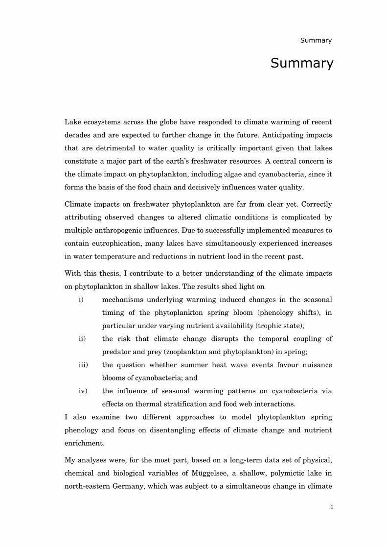
Lake ecosystems across the globe have responded to climate warming of recent

decades and are expected to further change in the future. Anticipating impacts

that are detrimental to water quality is critically important given that lakes

constitute a major part of the earth’s freshwater resources. A central concern is

the climate impact on phytoplankton, including algae and cyanobacteria, since it

forms the basis of the food chain and decisively influences water quality.

Climate impacts on freshwater phytoplankton are far from clear yet. Correctly

attributing observed changes to altered climatic conditions is complicated by

multiple anthropogenic influences. Due to successfully implemented measures to

contain eutrophication, many lakes have simultaneously experienced increases

in water temperature and reductions in nutrient load in the recent past.

With this thesis, I contribute to a better understanding of the climate impacts

on phytoplankton in shallow lakes. The results shed light on

i) mechanisms underlying warming induced changes in the seasonal

timing of the phytoplankton spring bloom (phenology shifts), in

particular under varying nutrient availability (trophic state);

ii) the risk that climate change disrupts the temporal coupling of

predator and prey (zooplankton and phytoplankton) in spring;

iii) the question whether summer heat wave events favour nuisance

blooms of cyanobacteria; and

iv) the influence of seasonal warming patterns on cyanobacteria via

effects on thermal stratification and food web interactions.

I also examine two different approaches to model phytoplankton spring

phenology and focus on disentangling effects of climate change and nutrient

enrichment.

My analyses were, for the most part, based on a long-term data set of physical,

chemical and biological variables of Müggelsee, a shallow, polymictic lake in

north-eastern Germany, which was subject to a simultaneous change in climate

Summary

2

and trophic state during the past three decades. To analyse the data, I

constructed a dynamic simulation model, implemented a genetic algorithm to

parameterize models, and applied statistical techniques of classification tree and

time-series analysis.

Results achieved with the dynamic simulation model indicated that the

mechanisms driving phytoplankton spring phenology in shallow lakes depend on

the trophic state. They also suggested that nutrient enrichment amplifies the

temporal advancement of the phytoplankton spring bloom, triggered by high

winter and spring temperatures. Also, warming decoupled the phytoplankton

from the zooplankton spring peak only under high nutrient supply. However, in

contrast to observations of other studies, this temporal predator-prey mismatch

did not cause the subsequent decline of the predator.

A novel approach to model phenology, which allows generating analytical

prediction, was parameterized based on experimental data. It proved useful to

assess the timings of population peaks of an artificially forced zooplankton-

phytoplankton system. Mimicking climate warming by lengthening the growing

period advanced algal blooms and consequently also peaks in zooplankton

abundance.

Investigating the reasons for the contrasting development of cyanobacteria

during two recent summer heat wave events, I found that anomalously hot

weather did not always promote cyanobacteria in the nutrient-rich lake studied.

The seasonal timing and duration of heat waves determined whether critical

thresholds of thermal stratification, decisive for cyanobacterial bloom formation,

were crossed.

In addition, the temporal patterns of heat wave events influenced the summer

abundance of some zooplankton species, which as predators may serve as a

buffer by suppressing phytoplankton bloom formation. Inter-annual differences

in water temperature during specific temporal windows explained most of the

contrasting responses of two zooplankton subgroups (cyclopoid copepods and

bosminids) to recent heat wave events.

In conclusion, this thesis adds to the growing body of evidence that lake

ecosystems have strongly responded to climatic changes of recent decades. It

Summary

3

reaches beyond many previous studies of climate impacts on lakes by focussing

on underlying mechanisms and explicitly considering multiple environmental

changes. Key findings show that while nutrients remain the primary agents that

determine the magnitude of phytoplankton blooms future climate change may

counteract successfully implemented measures to fight lake eutrophication, e.g.,

by favouring cyanobacteria. They also indicate that climate impacts are more

severe in nutrient-rich than in nutrient-poor lakes. Hence, to develop lake

management plans for the future, limnologists need to seek a comprehensive,

mechanistic understanding of overlapping effects of the multi-faceted human

footprint on aquatic ecosystems.

4

General introduction

5

General introduction

0.1 Concepts and motivation

Climate change impact on lake ecosystems—Aquatic and terrestrial ecosystems

across the globe have strongly responded to climate change of the recent past

(Parmesan and Yohe 2003; IPCC 2007). Lakes are considered especially suitable

indicators of ongoing climate change due to integration of changes occurring in

the entire catchment area and the prevalence of temperature driven processes

(Williamson et al. 2009). Climate induced changes have been recorded regarding

lake physics, chemistry and biology all over the world (Adrian et al. 2009;

Blenckner et al. 2007). A better mechanistic understanding of the observed

changes is crucial to anticipate the effects of expected further warming on lakes.

Detecting change that is detrimental to water quality is critically important

given that lakes constitute a major part of earth’s freshwater resources (Gleick

1996).

Phytoplankton blooms and multiple anthropogenic influences on lake

ecosystems—Phytoplankton is the principal primary producer in most lakes

forming the basis of the food chain (Wetzel 2001). Given suitable conditions

these microscopic organisms grow extremely rapidly building up considerable

biomass in a comparatively short time (‘blooms’) (e.g., Sommer and Lengfellner

2008). Certain phytoplankton species (cyanobacteria) float up to the water

surface developing green scums that can be observed as macroscopic phenomena

(Ibelings et al. 2003; Huisman et al. 2005). In addition, some of these species

produce toxins that may pose a threat to human health (Chorus 1999).

Due to their important role for water quality, phytoplankton blooms and the

underlying mechanisms have long been subjects of scientific interest (e.g., Lund

1950). Supply of large amounts of phosphorus (and to a lesser extent nitrogen)

to the water has been established as a major driving force of phytoplankton

blooms (Schindler 1974; Vollenweider and Kerekes 1982). This knowledge

allowed for effective lake management successfully containing eutrophication of

General introduction

6

lakes through reduction of nutrient inputs to freshwater bodies (Schindler

2006).

Climate impacts recorded in recent years have brought renewed interest in the

mechanisms underlying phytoplankton blooms. Meteorological variability has

been shown to affect the timing and magnitude of phytoplankton blooms in lakes

(see following paragraphs). Some of these studies concluded that ongoing and

future climate warming might counteract successfully achieved lake restoration

efforts of the past (Schindler 2006). However, the effects of climate change on

phytoplankton blooms are far from clear yet, with impacts varying depending on

ecosystem type, species involved and prevailing food web interactions (Straile

and Adrian 2000; Wiltshire et al. 2008; Adrian et al. 2009).

Numerous lakes have experienced climate change as well as a reduction in

nutrient loading (re-oligotrophication) at the same time (Jeppesen et al. 2005;

Köhler et al. 2005). Yet, up to now only few attempts have been made to

disentangle the effects of these simultaneous environmental changes (but see

Elliott et al. 2006; Feuchtmayr et al. 2009; Law et al. 2009). The results of this

thesis contribute to closing this important research gap. Accurately attributing

observed changes to climatic influences is crucial for the development of

effective lake management plans in the future.

Plankton spring phenology—The seasonal plankton growth pattern in temperate

lakes with moderately to high nutrient supply (eutrophic lakes) is marked by a

bloom of phytoplankton in spring (Sommer et al. 1986). Typically it is followed

by a population increase of zooplankton, which ultimately graze down the

phytoplankton producing a period of high water transparency in late

spring/early summer (the so-called ‘clear-water phase’). A synchronous

advancement in the phenology (timing) of these events concurrent with

increasing winter and spring water temperatures has been demonstrated for a

large number of lakes in the northern hemisphere (Gerten and Adrian 2000;

Straile 2002; Adrian et al. 2009). There have been, however, also studies

suggesting that the spring dynamics of phytoplankton and zooplankton species

are not necessarily accelerated in parallel (Winder and Schindler 2004a; de

Senerpont Domis et al. 2007a). This poses the risk of a mismatch in timing of

General introduction

7

prey availability and zooplankton reproduction, with potential detrimental

effects cascading up the food chain.

To anticipate phenology shifts under future climate warming and to assess the

threat of predator-prey mismatch, a mechanistic understanding of the spring

dynamics of plankton is required. Early studies investigating climate impacts on

plankton phenology have been purely observational. Important mechanistic

insights are beginning to emerge based on controlled experiments in laboratory

microcosms (e.g., Nicklisch et al. 2008) as well as mesocosms, which have the

advantage of better simulating natural conditions (e.g., Berger et al. 2007;

Sommer et al. 2007). Modelling the effect of climate warming on phytoplankton

spring blooms in lakes and reservoirs is another important approach to gain a

better mechanistic understanding of the processes involved (e.g., Tirok and

Gaedke 2007, Peeters et al. 2007a). However, few of these modelling studies

have dealt with shallow lakes so far, where mechanisms underlying the

phytoplankton spring dynamics are known to differ substantially from deep

lakes (see however Scheffer et al. 2001; Elliott et al. 2006). The modelling

approaches used in this thesis shed some light on these mechanisms and offer

promising avenues for phenology projections under future climate warming yet

to be undertaken.

Summer heat wave impact on phytoplankton—What we consider extreme

summer heat today could become average conditions by the end of this century

in many regions of the globe (Schär et al. 2004; Battisti and Naylor 2009). The

impact of past heat wave events on lakes therefore provide us with the

opportunity to study how these aquatic ecosystems could evolve under future

climate change. Central Europe has experienced extreme summer heat in recent

years, most prominently in 2003, which has strongly affected freshwater

ecosystems (Jankowski et al. 2006; Daufresne et al. 2007; Wilhelm and Adrian

2007, 2008).

The seasonal succession of plankton in lakes has been shown to be influenced

not only by the magnitude of temperature changes but also by their timing

within the season (Adrian and Straile 2000; Gerten and Adrian 2002, Wagner

and Benndorf 2007). This is to be expected for species with complex life-cycles,

General introduction

8

whose stages are known to be differentially sensitive to temperature (Moore et

al. 1996; Chen and Folt 2002). It might also stem from interactions between

temperature and other environmental factors (Giebelhausen and Lampert 2001),

in particular food availability and predation, which are of varying importance in

the course of the year (Sommer et al. 1986). The strong temperature anomalies

occurring during heat waves make these extreme events particularly suitable

opportunities to study the effects of different temporal patterns of warming on

lakes.

Due to their preference for high water temperatures and stable thermal

stratification, as generally prevailing under heat wave conditions, cyanobacteria

are often considered to be favoured by summer hot spells (Paerl and Huisman

2008). Heat waves have been recorded to increase the risk of cyanobacteria

bloom formation in some lakes (Jöhnk et al. 2008). However, whether this is a

general trend to be expected remains controversial; e.g., Wagner and Adrian

(2009) have recently demonstrated that the response of cyanobacteria to

prolonged and intensified stratification in a shallow lake is strongly species-

specific and depends on whether critical thresholds of nutrient (phosphorus and

nitrogen) concentrations have been passed. Despite the generally assumed

resistance of cyanobacteria to grazing, a few studies have also suggested that

food web interactions, susceptible to be strongly affected by heat waves as well,

can become decisive for bloom triggering (Vanni et al. 1990; Sarnelle 2007).

Taking the detailed seasonal pattern of meteorological forcing and potential food

web interactions into account, this thesis allows to narrowing down specific

circumstances under which future global warming is likely to favour

cyanobacteria blooms in shallow lakes.

0.2 Data basis, objectives and outline of thesis

Data basis—This thesis focuses on two types of phytoplankton blooms that are

typically observed in nutrient-rich, temperate lakes during the course of the

season (Sommer et al. 1986): diatom spring blooms and cyanobacteria summer

blooms (Fig. 0.1). While I concentrated on issues of bloom timing (phenology) in

spring (chapter 1 and 2), I was mainly interested in the magnitudes of blooms in

summer (chapter 3). The climate impact on summer zooplankton populations

General introduction

9

were also investigated (chapter 4), because food web interactions were revealed

as potential drivers of phytoplankton bloom formation.

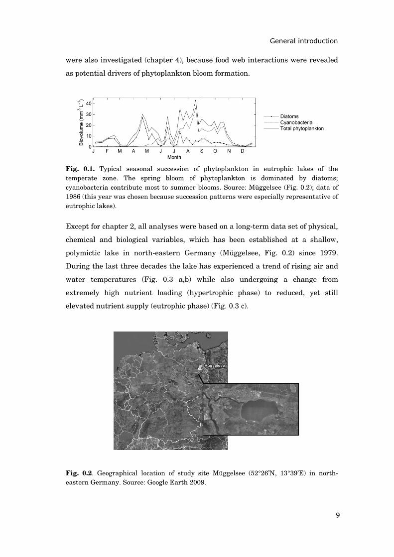
Fig. 0.1. Typical seasonal succession of phytoplankton in eutrophic lakes of the temperate zone. The spring bloom of phytoplankton is dominated by diatoms; cyanobacteria contribute most to summer blooms. Source: Müggelsee (Fig. 0.2); data of 1986 (this year was chosen because succession patterns were especially representative of eutrophic lakes).

Except for chapter 2, all analyses were based on a long-term data set of physical,

chemical and biological variables, which has been established at a shallow,

polymictic lake in north-eastern Germany (Müggelsee, Fig. 0.2) since 1979.

During the last three decades the lake has experienced a trend of rising air and

water temperatures (Fig. 0.3 a,b) while also undergoing a change from

extremely high nutrient loading (hypertrophic phase) to reduced, yet still

elevated nutrient supply (eutrophic phase) (Fig. 0.3 c).

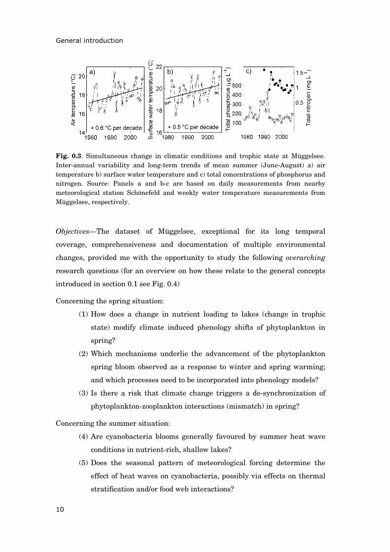
Fig. 0.2. Geographical location of study site Müggelsee (52°26’N, 13°39’E) in north-eastern Germany. Source: Google Earth 2009.

General introduction

10

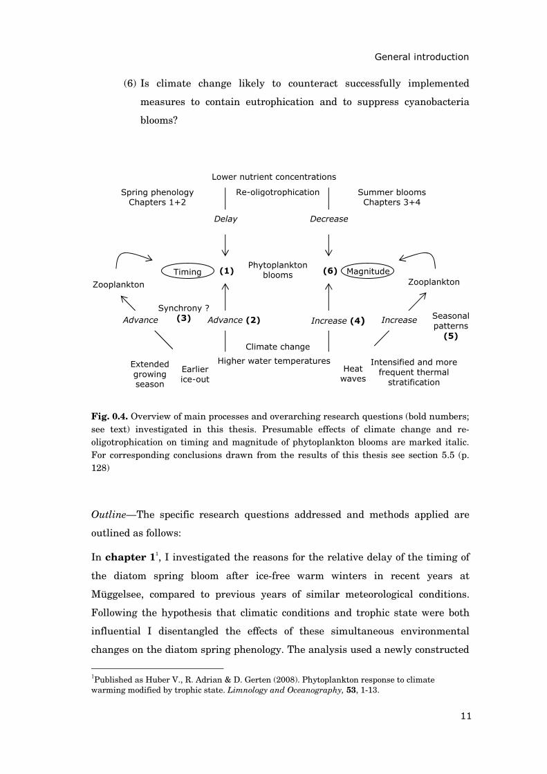
Fig. 0.3. Simultaneous change in climatic conditions and trophic state at Müggelsee. Inter-annual variability and long-term trends of mean summer (June-August) a) air temperature b) surface water temperature and c) total concentrations of phosphorus and nitrogen. Source: Panels a and b-c are based on daily measurements from nearby meteorological station Schönefeld and weekly water temperature measurements from Müggelsee, respectively.

Objectives—The dataset of Müggelsee, exceptional for its long temporal

coverage, comprehensiveness and documentation of multiple environmental

changes, provided me with the opportunity to study the following overarching

research questions (for an overview on how these relate to the general concepts

introduced in section 0.1 see Fig. 0.4)

Concerning the spring situation:

(1) How does a change in nutrient loading to lakes (change in trophic

state) modify climate induced phenology shifts of phytoplankton in

spring?

(2) Which mechanisms underlie the advancement of the phytoplankton

spring bloom observed as a response to winter and spring warming;

and which processes need to be incorporated into phenology models?

(3) Is there a risk that climate change triggers a de-synchronization of

phytoplankton-zooplankton interactions (mismatch) in spring?

Concerning the summer situation:

(4) Are cyanobacteria blooms generally favoured by summer heat wave

conditions in nutrient-rich, shallow lakes?

(5) Does the seasonal pattern of meteorological forcing determine the

effect of heat waves on cyanobacteria, possibly via effects on thermal

stratification and/or food web interactions?

a) b) c)

General introduction

11

(6) Is climate change likely to counteract successfully implemented

measures to contain eutrophication and to suppress cyanobacteria

blooms?

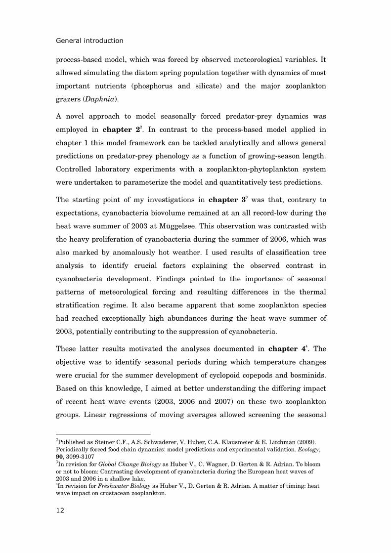
Fig. 0.4. Overview of main processes and overarching research questions (bold numbers; see text) investigated in this thesis. Presumable effects of climate change and re-oligotrophication on timing and magnitude of phytoplankton blooms are marked italic. For corresponding conclusions drawn from the results of this thesis see section 5.5 (p. 128)

Outline—The specific research questions addressed and methods applied are

outlined as follows:

In chapter 11, I investigated the reasons for the relative delay of the timing of

the diatom spring bloom after ice-free warm winters in recent years at

Müggelsee, compared to previous years of similar meteorological conditions.

Following the hypothesis that climatic conditions and trophic state were both

influential I disentangled the effects of these simultaneous environmental

changes on the diatom spring phenology. The analysis used a newly constructed

1Published as Huber V., R. Adrian & D. Gerten (2008). Phytoplankton response to climate warming modified by trophic state. Limnology and Oceanography, 53, 1-13.

Phytoplankton blooms

Climate change

Re-oligotrophicationSpring phenology Chapters 1+2

Summer blooms Chapters 3+4

Lower nutrient concentrations

Higher water temperatures

Timing Magnitude

Zooplankton Zooplankton

Intensified and more frequent thermal

stratification

Earlier ice-out

Advance Advance (2)

(1)

Delay

Increase (4)

(6)

Decrease

Synchrony ? (3)

Extended growing season

Heat waves

Increase Seasonal patterns

(5)

General introduction

12

process-based model, which was forced by observed meteorological variables. It

allowed simulating the diatom spring population together with dynamics of most

important nutrients (phosphorus and silicate) and the major zooplankton

grazers (Daphnia).

A novel approach to model seasonally forced predator-prey dynamics was

employed in chapter 22. In contrast to the process-based model applied in

chapter 1 this model framework can be tackled analytically and allows general

predictions on predator-prey phenology as a function of growing-season length.

Controlled laboratory experiments with a zooplankton-phytoplankton system

were undertaken to parameterize the model and quantitatively test predictions.

The starting point of my investigations in chapter 33 was that, contrary to

expectations, cyanobacteria biovolume remained at an all record-low during the

heat wave summer of 2003 at Müggelsee. This observation was contrasted with

the heavy proliferation of cyanobacteria during the summer of 2006, which was

also marked by anomalously hot weather. I used results of classification tree

analysis to identify crucial factors explaining the observed contrast in

cyanobacteria development. Findings pointed to the importance of seasonal

patterns of meteorological forcing and resulting differences in the thermal

stratification regime. It also became apparent that some zooplankton species

had reached exceptionally high abundances during the heat wave summer of

2003, potentially contributing to the suppression of cyanobacteria.

These latter results motivated the analyses documented in chapter 44. The

objective was to identify seasonal periods during which temperature changes

were crucial for the summer development of cyclopoid copepods and bosminids.

Based on this knowledge, I aimed at better understanding the differing impact

of recent heat wave events (2003, 2006 and 2007) on these two zooplankton

groups. Linear regressions of moving averages allowed screening the seasonal

2Published as Steiner C.F., A.S. Schwaderer, V. Huber, C.A. Klausmeier & E. Litchman (2009). Periodically forced food chain dynamics: model predictions and experimental validation. Ecology, 90, 3099-3107 3In revision for Global Change Biology as Huber V., C. Wagner, D. Gerten & R. Adrian. To bloom or not to bloom: Contrasting development of cyanobacteria during the European heat waves of 2003 and 2006 in a shallow lake. 4In revision for Freshwater Biology as Huber V., D. Gerten & R. Adrian. A matter of timing: heat wave impact on crustacean zooplankton.

General introduction

13

dynamics of zooplankton, water temperature and other environmental factors

for periods of highest correlations.

In the general discussion and concluding section, I discuss how the main results

of this thesis contribute to answering the overarching research questions raised

here, and how some of the analyses could be carried on to further improve the

proposed answers to these questions.

14

Chapter 1

Phytoplankton response to climate warming

modified by trophic state

______________________________

Published as Huber V., R. Adrian and D. Gerten (2008) Phytoplankton response

to climate warming modified by trophic state. Limnology and Oceanography,

53(1): 1-13.

Copyright 2008 by the American Society of Limnology and Oceanography, Inc.

1.1 Abstract

16

1.1 Abstract

We investigated the combined effect of reduced phosphorus supply and warmer

winter and spring conditions on the diatom spring bloom of a shallow lake.

Simulations with a simple dynamic model indicated that reduced ice cover and

increasing water temperatures resulted in a more intense and earlier bloom

independently of phosphorus concentrations. However, whereas the collapse of

the bloom was caused by silicate limitation under high phosphorus supply, it

was caused by Daphnia grazing under reduced phosphorus supply. This switch

from a bottom-up to a top-down driven collapse of the diatom spring bloom

explains why, despite similarly mild winters, the bloom was observed earlier

under high than under reduced phosphorus supply in the lake studied. Thus, an

assessment of possible changes in nutrient loading is crucial when anticipating

how phytoplankton could evolve under future climate warming.

Chapter 1

17

1.2 Introduction

Increasing anthropogenic pressure requires a better understanding of how

ecosystems react to multiple environmental stressors. During the last decades

many freshwater systems were subject to both a changing climate and changes

in trophic state due to reduced nutrient supply (Jeppesen et al. 2005). Yet, most

analyses of long-term data of these systems focused either on the effect of

climate change or on the effect of changes in trophic state. Few studies have

tried to disentangle the combined effect of rising temperatures and changing

nutrient supply on freshwater ecosystems (e.g., Horn 2003; Elliott et al. 2006).

Abiotic factors, influenced by climatic conditions and trophic state, are the

primary drivers of phytoplankton succession in spring (Sommer et al. 1986). In

lakes of the temperate zone, the phytoplankton spring bloom is predominantly

initiated by increasing light availability (Sommer 1994), which is directly

determined by solar radiation and day length and also indirectly depends on

specific lake features such as water transparency and depth. In deep lakes,

phytoplankton starts growing once strong mixing ceases and phytoplankton is

no longer constantly transported out of the euphotic zone (Peeters et al. 2007a).

In many shallow lakes, the phytoplankton spring bloom is initiated once the ice-

cover melts, inducing a change in the underwater regime of light and turbulence

(Adrian et al. 1999; Weyhenmeyer et al. 1999).

With the exception of very nutrient-rich lakes where grazer-resistant algae

dominate early in the year, the phytoplankton spring bloom then collapses

leading to a biomass minimum in late spring/early summer called the clear

water phase (Sommer et al. 1986). The collapse of the phytoplankton spring

bloom is attributed to different environmental factors. First, many studies have

shown that zooplankton grazing rates (mainly by Daphnia) often exceed algal

production rates in early summer, thus producing the clear water phase

(Lampert et al. 1986). Second, nutrient limitation (potentially combined with

increasing sinking losses) can induce a collapse of the phytoplankton bloom

before grazing becomes important (Lund 1950; Smayda 1971). And third, a

sharp increase in sinking losses due to the onset of stratification can also cause

1.2 Introduction

18

the collapse of the algal bloom if stable summer stratification develops in

moderately deep lakes (Winder and Schindler 2004b).

In lakes across the northern hemisphere, climate warming has induced forward

shifts in the timing of the phytoplankton spring maximum and the clear water

phase (Gerten and Adrian 2000; Straile 2002). On the one hand, these phenology

shifts have been attributed to a direct effect of increased water temperatures on

zooplankton grazers (Straile and Adrian 2000) and to a lesser extent to a direct

effect of increased water temperatures on phytoplankton growth (Adrian et al.

1999). On the other hand, warming more indirectly affects the phytoplankton

spring bloom through its effect on ice cover and the lake mixing regime (Adrian

et al. 1999; Winder and Schindler 2004b; Peeters et al. 2007a). Furthermore, it is

a classical result from eutrophication studies that in many lakes annual (or

seasonal) phytoplankton biomass is correlated to annual (seasonal) phosphorus

loading (Vollenweider and Kerekes 1982; Jeppesen et al. 2005). In addition to

the effect of nutrient availability on phytoplankton productivity, trophic state is

also known to affect the phytoplankton succession patterns, including the timing

of the phytoplankton spring bloom (Sommer 1994).

Disentangling the effect of climate and nutrients on phytoplankton growth has

proved challenging in the past. In a study of the effect of re-oligotrophication on

the phytoplankton growth in a drinking water reservoir, Horn (2003) found that

phytoplankton biomass did not decrease despite falling nutrient concentrations

and hypothesized that this was because of a change in spring overturn duration

dependent on weather conditions. In a modelling study, Elliott et al. (2006)

showed that the phytoplankton spring peak always occurred earlier under

higher temperatures, but it was species-specific as to whether increasing

nutrient concentrations delayed the peak or advanced it further. When Scheffer

et al. (2001) stated that the probability of a clear water phase increases with the

temperature of a lake, a controversy arose as to whether they had sufficiently

accounted for changes in the trophic state (and management regimes) of the

lakes studied (Jeppesen et al. 2003; Scheffer et al. 2003;Van Donk et al. 2003).

The shallow lake studied here, Müggelsee, provides an opportunity to gain a

better understanding of the combined effect of climate warming and changes in

Chapter 1

19

trophic state on the phytoplankton spring development. The lake experienced a

reduction of more than 50% in both total phosphorus and total nitrogen loading

from a hypertrophic period, 1979–1990, to a eutrophic period, 1997–2003

(Köhler et al. 2005). In spring, phytoplankton is dominated by diatoms in this

lake, and phosphorus and silicate are the potentially limiting factors, whereas

nitrogen limitation most likely only plays a role in the summer (Köhler et al.

2000; Köhler et al. 2005). Climate-induced changes of physical lake features and

resulting phenology shifts in the plankton community are well documented for

this lake (Adrian et al. 1999; Straile and Adrian 2000). In particular, a forward

shift of the phytoplankton spring bloom of about 1 month was found

concurrently with earlier ice break-up dates from 1979–1987 to 1988–2003

(Gerten and Adrian 2000; Adrian et al. 2006). However, although ice break-up

dates were generally a good predictor of the timing of the phytoplankton spring

bloom, the bloom occurred relatively late in recent mild years with early ice-out.

In this study, we asked whether the climate signal detected in the

phytoplankton time series was altered by decreasing phosphorus loading to the

lake. Specifically, we investigated whether the relative delay of the

phytoplankton spring bloom in recent years could be attributed to the observed

change in trophic state. Based on long-term data (1979–2005) of physical,

chemical, and biological variables, we constructed a deterministic model that

simulates the dynamics of diatom biovolume, the potentially limiting nutrients

(silicate and phosphorus), and Daphnia grazing in winter and spring. Using this

model, we performed simulation experiments to explore how increased water

temperatures and reduced ice cover affected the timing and intensity of the

diatom spring bloom under conditions of high and reduced phosphorus loading

(hypertrophic and eutrophic phase). These model simulations suggested a switch

in bloom collapse mechanisms, rendering the phytoplankton response to climate

warming strongly dependent on trophic state.

1.3 Methods

Study site—Müggelsee is a shallow, polymictic lake situated in the southeast of

Berlin (52°26’N, 13°39’E). It spans an area of 7.3 km2 with a mean depth of 4.9

m and a maximum depth of 7.9 m. The lake is moderately flushed by the river

1.3 Methods

20

Spree with a retention time of approximately 6–8 weeks (Köhler et al. 2005). The

climate at this lake is governed by maritime and continental influences. Winter

climate shows a high degree of inter-annual variability, with the monthly mean

air temperature in January, the coldest month, varying within the approximate

range of -7°C to +5°C (Adrian and Hintze 2000). Ice-cover duration varied

between 0 days and 125 days in 1979–2005 with an average ice cover of 43 ± 33

SD days. Additional information on physical and limnological characteristics of

Müggelsee is documented in Driescher

et al. (1993).

Data basis—From 1979 to 2005, water samples for nutrient and plankton

analysis were taken weekly during the growing season and biweekly during

winter. A detailed description of the sampling methodologies and sample

processing is given in Gerten and Adrian (2000). Time-series of aggregated

biovolume of total phytoplankton and aggregated biovolume of diatoms

(Bacillariophyceae) were used in this study. For model development, we focussed

on diatoms because these constituted about 81 % of total phytoplankton

biovolume in Müggelsee during the spring peak (Fig. 1.1A). As grazers, only

daphnids (mainly Daphnia galeata, Daphnia hyalina, Daphnia cucullata, and

their hybrids) were considered in the model, however, other zooplankton groups

(ciliates, cyclopoid, and calanoid copepods) were accounted for in a

supplementary screening of factors that potentially influence the phenology of

diatoms. Long-term records of physical factors (water temperature, ice cover,

global radiation, light extinction) and weekly measurements of nutrients (total

phosphorus concentration [TP] and dissolved silicate concentration [DSi]) were

used as forcing variables in the model or for the purpose of parameter

estimation (cf. Table 1.1). Water temperatures were hourly means (8 - 9 h)

recorded daily near the lake surface at 0.3 m depth (from September 2002

onwards at 1–2 m depth during winter and at 0.5 m during spring and summer).

Ice cover was assessed daily categorizing whether the lake was fully (>80 % of

the lake surface) or partially covered with ice. Long-term records of mean daily

global radiation were provided by Deutscher Wetterdienst for the station in

Potsdam (52°04’N, 13°06’E) for 1979–2002; from 2003–2005 records from a

Chapter 1

21

measurement station at the shore of Müggelsee were used. Incident

photosynthetically available radiation (PAR) was considered to be 43% of global

radiation. This was based on the assumption that on average 7% of global

radiation are reflected at the water surface (estimated from measurements at

Müggelsee in spring 2002, 2004, 2005, n=262) and that 46% of global radiation

are photosynthetically available (Köhler et al. 2000). Light extinction coefficients

were estimated based on light measurement in the water column (0-5 m) during

1993 – 2003 and transmittance through ice was assessed using measurements

in the winter of 1995/1996.

Definition of phenology events—Ice-out date was defined as the week (or day of

the year for model analysis) when the lake was free of all ice in spring. The

timing of the diatom spring bloom was defined as the week (day of the year)

when maximal biovolume of diatoms was observed after ice-out in spring. In

years when several local maxima were observed (occurring in 6 out of 27 years)

the timing of the highest peak was considered. The maximal biovolume was

considered as the magnitude of the bloom. Also, we defined the end of the bloom

as the week (day of the year) when minimal diatom biovolume was observed

after the spring peak. This coincided with the clear water phase (defined as time

of highest Secchi depth in late spring) during most years. We defined the

intensity of the bloom as the mean biovolume from the beginning of the year

until the end of the bloom. The timing of the Daphnia spring peak was defined

as the first, clearly distinguishable maximum in spring (with densities >= 68 ind

L-1).

Model core—The spring diatom phenology model used here builds upon a

phytoplankton growth model for a closed system proposed by Diehl et al. (2005)

and modified according to an approach used by Klausmeier et al. (2004). It is a

point-like model based on the assumption that the whole water column is well-

mixed and phytoplankton is homogenously distributed in the water column,

which is realistic for shallow, polymictic Müggelsee in spring. Our model is

constructed in order to simulate diatom dynamics in winter and spring only (Jan

– mid-Jun). The core of the model consists of four differential equations (Eqs. 1-

4) describing changes in diatom biovolume and the dynamics of the potentially

1.3 Methods

22

limiting nutrients phosphorus and silicate (definitions and units of state

variables, parameters, and forcing variables are summarized in Table 1.1).

ADcTFzvSiQIT

dtdA

DD ⎟⎟⎠

⎞⎜⎜⎝

⎛⎟⎠⎞

⎜⎝⎛ +−= )(),,,(μ (1)

QSiQITPH

PTFdtdQ

PA ),,,()(max μρ −

+= (2)

( ) APH

PTFQAPPrdtdP

PAtotP +

−−−= )(maxρ (3)

( ) ),,,( SiQITAQAQSiSrdtdSi

SiSitotSi μ−−−= (4)

Biovolume concentration of diatoms A (mm3 L-1) increases through temperature,

light, and nutrient dependent growth (integrating all internal processes such as

primary production, respiration, exudation, and lysis) and decreases through

sedimentation and temperature dependent Daphnia grazing. Sedimentation loss

rate was calculated as the ratio of sinking velocity v (m day-1) to mixing depth z

(m). For simplicity, we assumed that filtration rates are independent of prey

density (type I functional response) so that Daphnia grazing loss rate is the

product of clearance rate cD (L ind-1 day-1) and Daphnia density D (ind L-1).

The temperature dependence of grazing and other Daphnia related process rates

(see below) were described by the Q10-rule:

10( ) 2refT TC

DF T−⎛ ⎞

⎜ ⎟⎜ ⎟°⎝ ⎠= (5)

where T (°C) is the seasonally changing water temperature and Tref (°C) is the

reference temperature. This is an experimentally backed approach (Norberg and

DeAngelis 1997), commonly used in minimal models of phytoplankton-

zooplankton interaction (Scheffer et al. 2001; Peeters et al. 2007a). The algal

growth rate, which is dependent on water temperature, light intensity I (W m-2),

silicate concentration Si (mg L-1), and phosphorus cell quota Q (μg P mm-3), was

calculated as

( ))(),(min),()(),,,( 321max QLSiLITLTFSiQIT Aμμ = (6)

where µmax (day-1) is the maximum specific growth rate, L1, L2, and L3 are

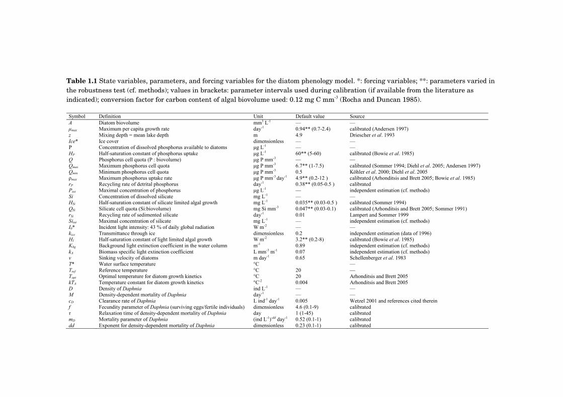
Table 1.1 State variables, parameters, and forcing variables for the diatom phenology model. *: forcing variables; **: parameters varied in the robustness test (cf. methods); values in brackets: parameter intervals used during calibration (if available from the literature as indicated); conversion factor for carbon content of algal biovolume used: 0.12 mg C mm-3 (Rocha and Duncan 1985). Symbol Definition Unit Default value Source A Diatom biovolume mm3 L-1 — — μmax Maximum per capita growth rate day-1 0.94** (0.7-2.4) calibrated (Andersen 1997) z Mixing depth = mean lake depth m 4.9 Driescher et al. 1993 Ice* Ice cover dimensionless — — P Concentration of dissolved phosphorus available to diatoms μg L-1 — — HP Half-saturation constant of phosphorus uptake μg L-1 60** (5-60) calibrated (Bowie et al. 1985) Q Phosphorus cell quota (P : biovolume) μg P mm-3 — — Qmax Maximum phosphorus cell quota μg P mm-3 6.7** (1-7.5) calibrated (Sommer 1994; Diehl et al. 2005; Andersen 1997) Qmin Minimum phosphorus cell quota μg P mm-3 0.5 Köhler et al. 2000; Diehl et al. 2005 ρmax Maximum phosphorus uptake rate μg P mm-3 day-1 4.9** (0.2-12 ) calibrated (Arhonditsis and Brett 2005; Bowie et al. 1985) rP Recycling rate of detrital phosphorus day-1 0.38** (0.05-0.5 ) calibrated Ptot Maximal concentration of phosphorus μg L-1 — independent estimation (cf. methods) Si Concentration of dissolved silicate mg L-1 — — HSi Half-saturation constant of silicate limited algal growth mg L-1 0.035** (0.03-0.5 ) calibrated (Sommer 1994) QSi Silicate cell quota (Si:biovolume) mg Si mm-3 0.047** (0.03-0.1) calibrated (Arhonditsis and Brett 2005; Sommer 1991) rSi Recycling rate of sedimented silicate day-1 0.01 Lampert and Sommer 1999 Sitot Maximal concentration of silicate mg L-1 — independent estimation (cf. methods) I0* Incident light intensity: 43 % of daily global radiation W m-2 — — kice Transmittance through ice dimensionless 0.2 independent estimation (data of 1996) HI Half-saturation constant of light limited algal growth W m-2 3.2** (0.2-8) calibrated (Bowie et al. 1985) Kbg Background light extinction coefficient in the water column m-1 0.89 independent estimation (cf. methods) kA Biomass specific light extinction coefficient L mm-3 m-1 0.07 independent estimation (cf. methods) v Sinking velocity of diatoms m day-1 0.65 Schellenberger et al. 1983 T* Water surface temperature °C — Tref Reference temperature °C 20 — Topt Optimal temperature for diatom growth kinetics °C 20 Arhonditsis and Brett 2005 kTA Temperature constant for diatom growth kinetics °C-2 0.004 Arhonditsis and Brett 2005 D Density of Daphnia ind L-1 — — M Density-dependent mortality of Daphnia day-1 — — cD Clearance rate of Daphnia L ind-1 day-1 0.005 Wetzel 2001 and references cited therein f Fecundity parameter of Daphnia (surviving eggs/fertile individuals) dimensionless 4.6 (0.1-9) calibrated τ Relaxation time of density-dependent mortality of Daphnia day 1 (1-45) calibrated mD Mortality parameter of Daphnia (ind L-1)-dd day-1 0.52 (0.1-1) calibrated dd Exponent for density-dependent mortality of Daphnia dimensionless 0.23 (0.1-1) calibrated

1.3 Methods

24

limitation functions described below and FA(T) is the temperature function used

for diatom growth constants and process rates. For the latter we adopted the

optimum curve suggested by Arhonditsis and Brett (2005)

( )( )2exp)( optAA TTkTTF −−= (7)

where kTA (°C -2) describes the strength of the temperature effect and Topt (°C) is

the optimal temperature for diatom growth processes. Co-limitation of several

resources was accounted for by using Liebig’s minimum function for phosphorus

and silicate that are considered strictly essential resources (Tilman 1982). Light

was assumed to be an interactive essential resource (Rhee and Gotham 1981;

Post et al. 1985), and, therefore, a multiplicative approach was adopted.

Extinction was calculated according to the Lambert-Beer law including self-

shading of algae. Based on this, mean underwater light intensity I (W m-2) was

determined by integrating over mixing depth:

( ) ( )( )zAkK

zAkKIdssAkKI

zI

Abg

Abgoz

Abg )()(exp1

)(exp1

00 +

+−−=+−= ∫ (8)

where Kbg (m-1) is the background extinction coefficient, and kA (L mm-3 m-1) the

diatom biovolume specific extinction coefficient. The incident light I0 (W m-2) was

reduced to kiceI0 when the lake was at least partially ice-covered. Light limitation

of diatom growth was modelled using a Monod-approach:

IHTFIITL

IA +=

)(),(1 (9)

where HI (W m-2) is the half-saturation constant for light-limited growth, which

is assumed to change with temperature. This temperature dependency of HI

assures that strongly light-limited growth is temperature independent (the

initial slope of the hyperbolic curve is constant), as suggested by empirical

studies of the interaction of light and temperature on algal growth (Post et al.

1985). We checked that this affected the growth in colder and warmer years

similarly and, thus, was not an important control for the differences between

colder and warmer years. Since silicate is not stored by phytoplankton, we

assumed a constant silicate cell quota QSi (mg Si mm-3) and also modelled the

diatom growth dependency on silicate availability with a Monod-equation

(Sommer 1994):

Chapter 1

25

SiHSiSiL

Si +=)(2 (10)

where HSi (mg L-1) is the half-saturation constant for silicate-limited growth. In

contrast, growth dependency on a variable phosphorus cell quota (Q) was

accounted for by using a Droop-model approach (Droop 1983), modified as

suggested by Wernicke and Nicklisch (1986):

( ) ⎟⎟⎠

⎞⎜⎜⎝

⎛⎟⎟⎠

⎞⎜⎜⎝

⎛⎟⎟⎠

⎞⎜⎜⎝

⎛−−−= 12lnexp1)(

min3 Q

QQL (11)

Here, growth is increasingly limited by phosphorus shortage (L3(Q) approaches

0) when the cell quota Q approaches the minimum cell quota Qmin, while

phosphorus limitation decreases as Q increases (L3(Q) approaches 1). The

phosphorus cell quota increases through phosphorus uptake and decreases

through algal growth (Eq. 2). To model the relationship between dissolved

phosphorus available to diatoms P (μg L-1) and uptake rate, we applied

Michaelis-Menten kinetics, where ρmax (μg P mm-3 day-1) is the maximal

phosphorus uptake rate and HP (μg L-1) the half-saturation constant for

phosphorus uptake (Eqs. 2 and 3).

Phenomenological approach to nutrient dynamics—The concentration of

dissolved phosphorus available to diatoms increases through recycling of detrital

phosphorus with a recycling rate of rP (day-1) and decreases through phosphorus

uptake (Eq. 3). Instead of explicitly considering the processes that lead to the

recycling of nutrients such as the remineralization of phosphorus trapped in

sedimented algae and the cycling of phosphorus through grazing, we chose a

phenomenological approach and considered a closed system with a maximal

phosphorus concentration of Ptot (μg L-1). We neglected all phosphorus potentially

stored in grazers, so that the pool of recyclable phosphorus could be calculated

as the phosphorus, which was neither dissolved in the water column nor

included in algae (Ptot - P - QA). To estimate the maximal phosphorus

concentration potentially available to diatoms (Ptot), we used an empirical

relationship based on diatom and phosphorus data measured during winter and

spring 1979-2005. In fact, the annual mean diatom biovolume between the

beginning of the year and the end of the bloom (Abloom) and the annual mean total

1.3 Methods

26

phosphorus concentration during the same period (TPbloom) showed a significant

linear relationship:

Abloom = 0.14 TPbloom -7.37 (n=27, R2=0.64, p<0.001) (12)

We then assumed that a fixed amount of phosphorus (given by the interception

of the regression line with x-axis TP*=52 μg L-1) was locked in other

compartments (such as bacteria, other phytoplankton species, zooplankton, and

phosphorus bound to iron or calcite) and not available to diatoms. Thus, we

calculated the maximal phosphorus concentration (Ptot) available to diatoms each

year as the difference between TPbloom and TP*.

In a similar approach, dissolved silicate was assumed to increase through the

recycling of sedimented silicate with a recycling rate of rSi (day-1) and to decrease

through growth of diatoms with a fixed silicate cell quota QSi (Eq. 4). The pool of

recyclable silicate was calculated analogous to the pool of recyclable phosphate

(Sitot - Si - QSiA), with the difference that the maximal silicate concentration (Sitot)

in the model was estimated as the maximal concentration of DSi observed in

Müggelsee for each year.

The Daphnia sub-model—Several studies have found that the development of

Daphnia biomass in spring is driven primarily by temperature and relatively

independent of food availability (Straile and Adrian 2000; Gerten and Adrian

2000; Benndorf et al. 2001). When food becomes limiting in late spring and early

summer other algal groups besides diatoms (mainly Cryptophyceae and

Chlorophyceae) contribute to Daphnia food in Müggelsee. We, therefore, did not

couple Daphnia to simulated diatom biovolume and included possible food

limitation of Daphnia later in the season only implicitly through density-

dependent mortality. (In fact, the phenomenological approach presented here

resulted in a better model performance than a classical predator-prey approach,

with Daphnia coupled to diatoms.) Density-dependent mortality M (day-1) was

simulated using a general formulation adopted from Tirok and Gaedke (2007):

( )MDmdt

dM ddD −=

τ1

(13)

where mD ((ind L-1)-dd day-1) and dd (dimensionless) modulate the strength of the

density-dependent mortality and τ (day) corresponds to a relaxation time.

Chapter 1

27

Reproduction was calculated as a function of temperature dependent egg

development time dev(T) (day) based on the empirical relationship given by

Bottrell et al. (1976):

( )( )2)ln(3414.0)ln(2193.03956.3exp)( TTTdev −+= (14)

Using a fecundity parameter f (dimensionless), which roughly combines the

proportion of reproductively active individuals in the population with the

number of eggs per individual, the rate of change in Daphnia population density

D (ind L-1) was then calculated following Eq. 15:

DMTFTdev

fdtdD

D ⎟⎟⎠

⎞⎜⎜⎝

⎛−= )(

)( (15)

where FD(T) corresponds to the Q10 rule (Eq. 5).

Model initialization—Since our model did not allow simulating the whole

annual cycle, it had to be initiated each year. Initial values for diatom biovolume

concentration A0 were the mean of the last observation in the previous year and

the first observation in the current year. The phosphorus cell quota Q was

initially set to the maximal cell quota Qmax. The initial concentration of dissolved

phosphorus available to diatoms P0 (dissolved silicate Si0) was calculated as the

difference between the maximal phosphorus (silicate) concentration Ptot (Stot) and

phosphorus (silicate) initially stored in diatoms A0Qmax (A0QSi). Initial values for

Daphnia densities D0 corresponded to first observations of each year, and

density-dependent mortality M was set to the steady state condition mDD0dd.

Parameter calibration, model validation, and robustness against changes in

parameters—Part of the parameter values were independently estimated from

the data or directly taken from the literature (as indicated in Table 1.1). The

other parameters (four parameters of the Daphnia sub-model and eight

parameters of the core model describing the algal-nutrient dynamics) were

calibrated, if possible based on biologically plausible intervals as documented in

the literature (cf. Table 1.1). For this purpose, we split the data set into two sub-

periods: 1979-1992 for calibration and 1993-2005 for validation. We used a

genetic algorithm (adopted from Tietjen and Huth 2006) to efficiently search the

parameter space and to find the parameter set that optimizes the fit between

1.3 Methods

28

the model and the data (for details on the calibration procedure see Appendix).

For model validation we assessed model performance as measured by Willmott’s

(1982) index of agreement (IoA). It describes the modelling quality with respect

to the variance and the mean ( )O of the observations. IoA = 0 indicates complete

disagreement between predicted (Pi) and observed values (Oi), while IoA = 1

indicates complete agreement:

( )∑

∑

=

=

−+−

−−= n

iii

n

iii

OOOP

OPIoA

1

2

1

2)(1 (16)

The index was calculated for the calibration (1979-1992) and the validation

period (1993-2005) separately. The data used were (a) the observed and

predicted diatom biovolume and Daphnia abundance (IoAb) and b) the observed

and predicted timing of the diatom and Daphnia spring peak (IoAt). In the

former case, we used all weekly measurements until the end of the simulation

period (mid-Jun) summing over all years considered (O is not the seasonal but

the long-term mean). We thereby assessed the ability of the model to reproduce

the observed seasonal dynamics during winter and spring. In the latter case,

calculations were based on yearly estimations of the timing of the peak.

The robustness of the model was tested by varying the calibrated parameters of

the diatom model (Table 1.1) by +/- 20% as suggested by Omlin et al. (2001) for

moderately inaccurate parameters. Timing and intensity of the simulated

diatom blooms were then calculated for all of these parameter combinations (n=

1944; three parameter values were excluded that lay outside the biologically

plausible interval) and the resulting distributions depicted with boxplots (Fig.

1.2 A, B).

Control run and simulation experiments—In order to assess how climate

warming affected diatom spring phenology under different trophic states, we ran

a number of simulation experiments. The validated model, which was forced by

current environmental factors (ice cover, water temperature, global radiation,

maximal phosphorus, and silicate availability) served as a control (abbreviated

‘C’). Scenarios consisted of setting one or several of these environmental forcing

Chapter 1

29

factors to data of extreme years while using current data for the remaining

factors.

The effect of missing ice cover and increased water temperatures (warming

scenario abbreviated ‘W’) was assessed by running the model for every year on

climate data from 1990, but keeping current data of global radiation and

nutrient availability. The winter and spring (Jan-May) of 1990 was

exceptionally warm with average water temperatures being 1.6 °C higher than

the long-term mean of 1979-2005.

Hypertrophic conditions (abbreviated ‘HYP’) were simulated by calculating the

upper limit of phosphorus concentrations available (Ptot) based on the maximum

of the observed mean total phosphorus concentrations in spring (TPbloom = 135 μg

L-1 in 1988, see Fig. 1.1A). Likewise, eutrophic conditions (abbreviated ‘EU’)

were simulated based on the minimum of observed mean total phosphorus

concentrations in spring (TPbloom = 62 μg L-1 in 2001, see Fig. 1.1A). Maximum

and minimum of mean total phosphorus concentrations observed in the time-

series were assumed to represent two different trophic states according to

Köhler et al. (2005). These authors classified a hypertrophic (1979-1990),

transient (1991-1996) and eutrophic phase (1997-2003) at Müggelsee based on

data of external and internal nutrient loading.

We also investigated the effect of silicate and the effect of Daphnia grazing on

diatom spring phenology. Silicate limitation was turned off (abbreviated ‘NSi’)

by fixing the silicate limitation factor at 1. Daphnia grazing was turned off

(abbreviated ‘ND’) by setting the Daphnia grazing constant to 0. Results of

simulation experiments were depicted with boxplots showing the inter-annual

variability (1979-2005) of the intensity (Fig. 1.3) and timing (Fig. 1.4) of the

diatom spring bloom under different scenarios. All model simulations and

statistical tests were performed using Matlab 6.5 and 7.0 (MathWorks, Inc.).

1.4 Results

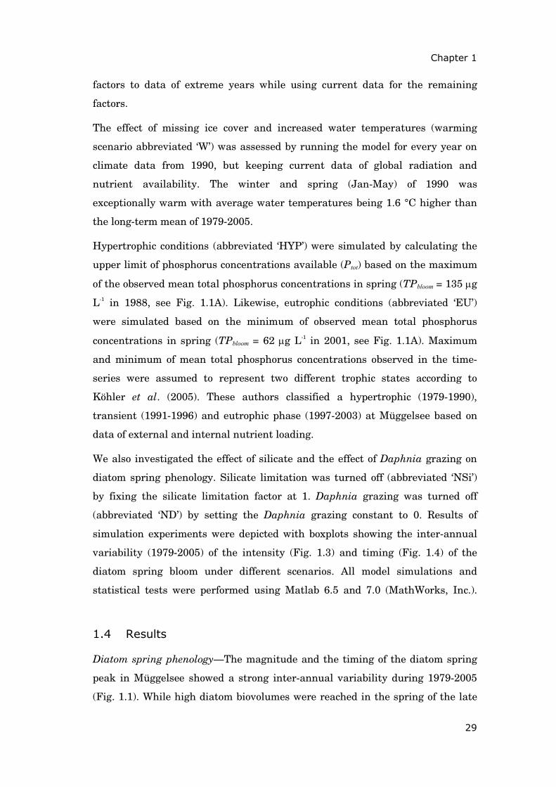
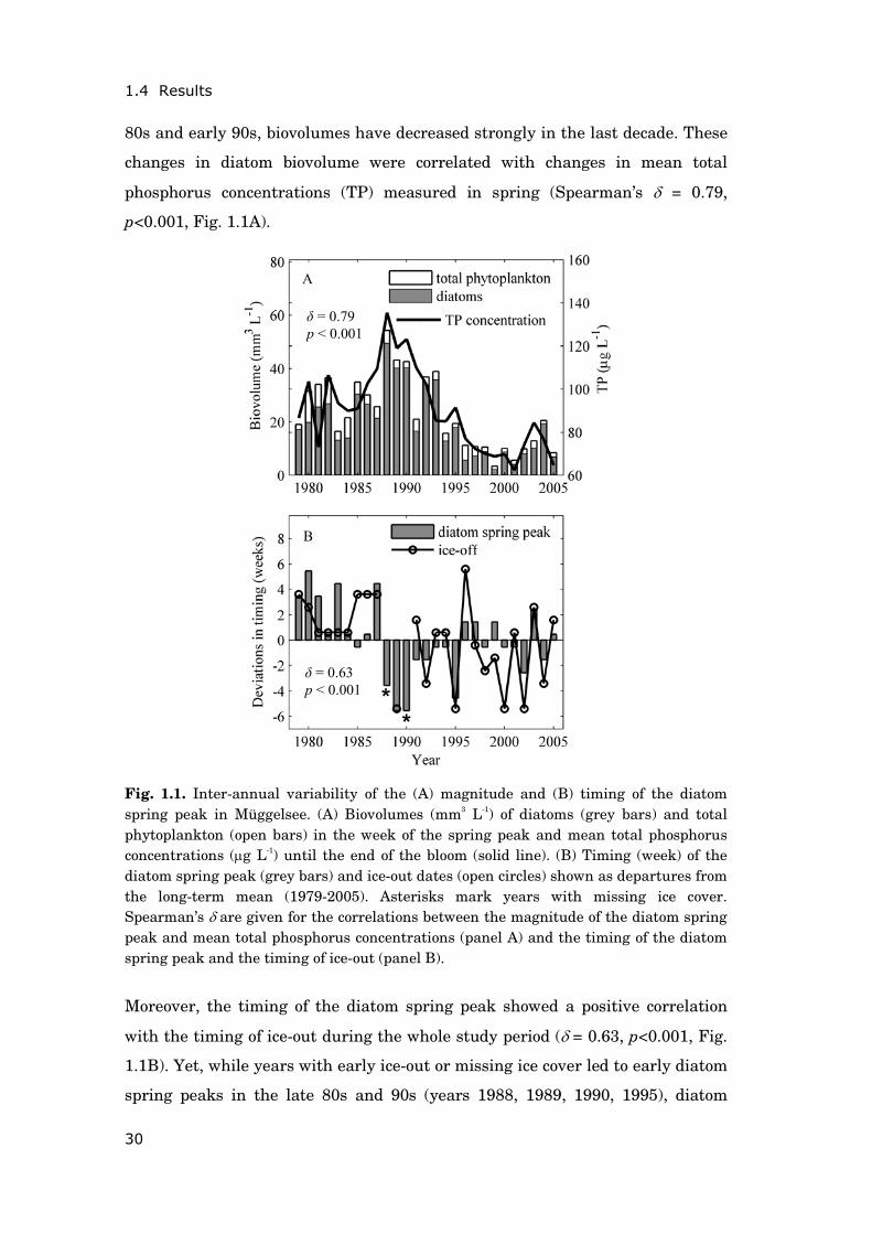
Diatom spring phenology—The magnitude and the timing of the diatom spring

peak in Müggelsee showed a strong inter-annual variability during 1979-2005

(Fig. 1.1). While high diatom biovolumes were reached in the spring of the late

1.4 Results

30

80s and early 90s, biovolumes have decreased strongly in the last decade. These

changes in diatom biovolume were correlated with changes in mean total

phosphorus concentrations (TP) measured in spring (Spearman’s δ = 0.79,

p<0.001, Fig. 1.1A).

Fig. 1.1. Inter-annual variability of the (A) magnitude and (B) timing of the diatom spring peak in Müggelsee. (A) Biovolumes (mm3 L-1) of diatoms (grey bars) and total phytoplankton (open bars) in the week of the spring peak and mean total phosphorus concentrations (μg L-1) until the end of the bloom (solid line). (B) Timing (week) of the diatom spring peak (grey bars) and ice-out dates (open circles) shown as departures from the long-term mean (1979-2005). Asterisks mark years with missing ice cover. Spearman’s δ are given for the correlations between the magnitude of the diatom spring peak and mean total phosphorus concentrations (panel A) and the timing of the diatom spring peak and the timing of ice-out (panel B).

Moreover, the timing of the diatom spring peak showed a positive correlation

with the timing of ice-out during the whole study period (δ = 0.63, p<0.001, Fig.

1.1B). Yet, while years with early ice-out or missing ice cover led to early diatom

spring peaks in the late 80s and 90s (years 1988, 1989, 1990, 1995), diatom

**

δ = 0.63 p < 0.001

A

δ = 0.79 p < 0.001

B

Chapter 1

31

spring peaks occurred relatively late despite early ice-out in recent years (2000

and 2002). Correlation analysis did not reveal any significant relationship

between the timing of ice-out and the magnitude of the diatom spring peak (δ =

0.05, p>0.1) nor between the mean total phosphorus concentrations in spring

and the timing of the diatom spring peak (δ = -0.22, p>0.1). We applied the

diatom phenology model to investigate these relationships further.

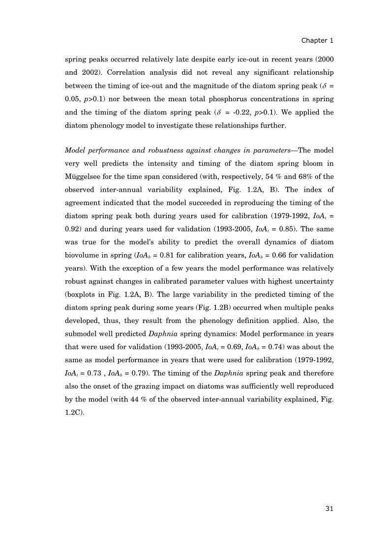
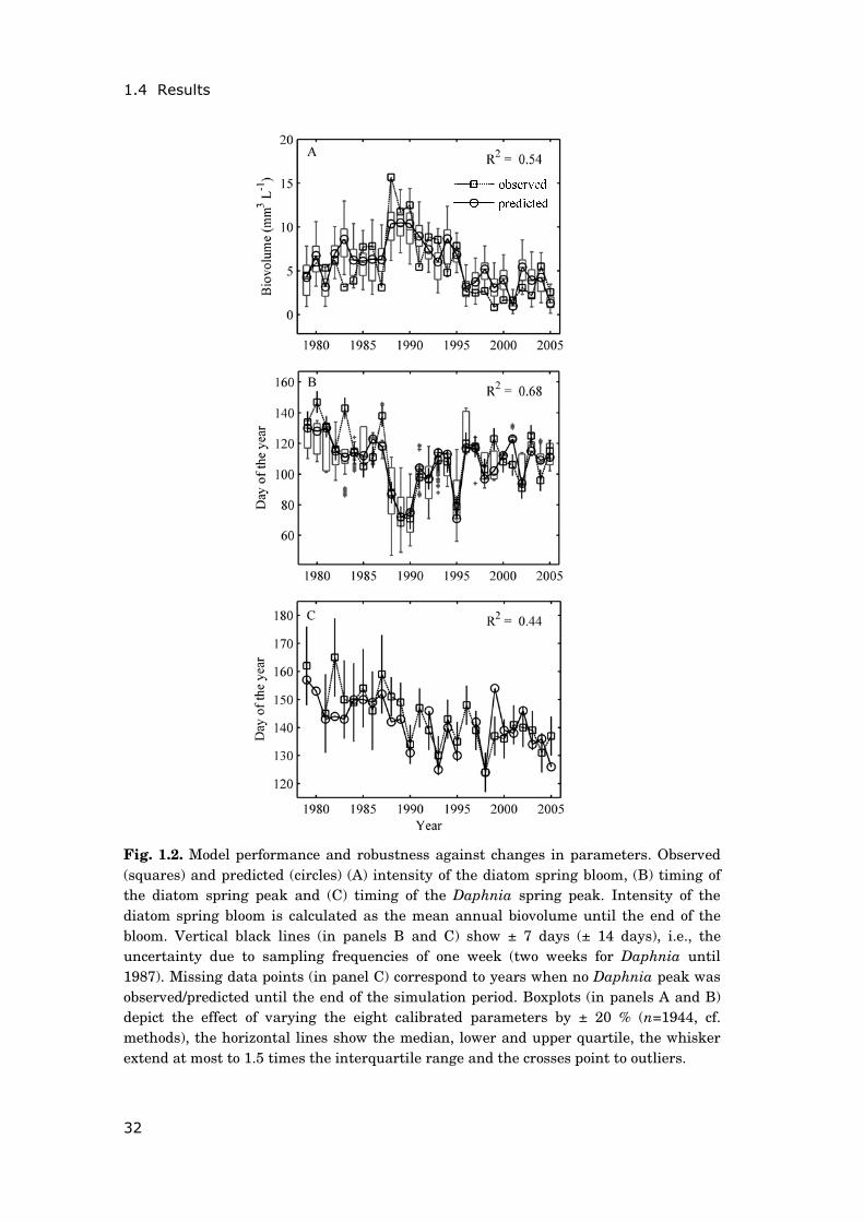
Model performance and robustness against changes in parameters—The model

very well predicts the intensity and timing of the diatom spring bloom in

Müggelsee for the time span considered (with, respectively, 54 % and 68% of the

observed inter-annual variability explained, Fig. 1.2A, B). The index of

agreement indicated that the model succeeded in reproducing the timing of the

diatom spring peak both during years used for calibration (1979-1992, IoAt =

0.92) and during years used for validation (1993-2005, IoAt = 0.85). The same

was true for the model’s ability to predict the overall dynamics of diatom

biovolume in spring (IoAb = 0.81 for calibration years, IoAb = 0.66 for validation

years). With the exception of a few years the model performance was relatively

robust against changes in calibrated parameter values with highest uncertainty

(boxplots in Fig. 1.2A, B). The large variability in the predicted timing of the

diatom spring peak during some years (Fig. 1.2B) occurred when multiple peaks

developed, thus, they result from the phenology definition applied. Also, the

submodel well predicted Daphnia spring dynamics: Model performance in years

that were used for validation (1993-2005, IoAt = 0.69, IoAb = 0.74) was about the

same as model performance in years that were used for calibration (1979-1992,

IoAt = 0.73 , IoAb = 0.79). The timing of the Daphnia spring peak and therefore

also the onset of the grazing impact on diatoms was sufficiently well reproduced

by the model (with 44 % of the observed inter-annual variability explained, Fig.

1.2C).

1.4 Results

32

Fig. 1.2. Model performance and robustness against changes in parameters. Observed (squares) and predicted (circles) (A) intensity of the diatom spring bloom, (B) timing of the diatom spring peak and (C) timing of the Daphnia spring peak. Intensity of the diatom spring bloom is calculated as the mean annual biovolume until the end of the bloom. Vertical black lines (in panels B and C) show ± 7 days (± 14 days), i.e., the uncertainty due to sampling frequencies of one week (two weeks for Daphnia until 1987). Missing data points (in panel C) correspond to years when no Daphnia peak was observed/predicted until the end of the simulation period. Boxplots (in panels A and B) depict the effect of varying the eight calibrated parameters by ± 20 % (n=1944, cf. methods), the horizontal lines show the median, lower and upper quartile, the whisker extend at most to 1.5 times the interquartile range and the crosses point to outliers.

Chapter 1

33

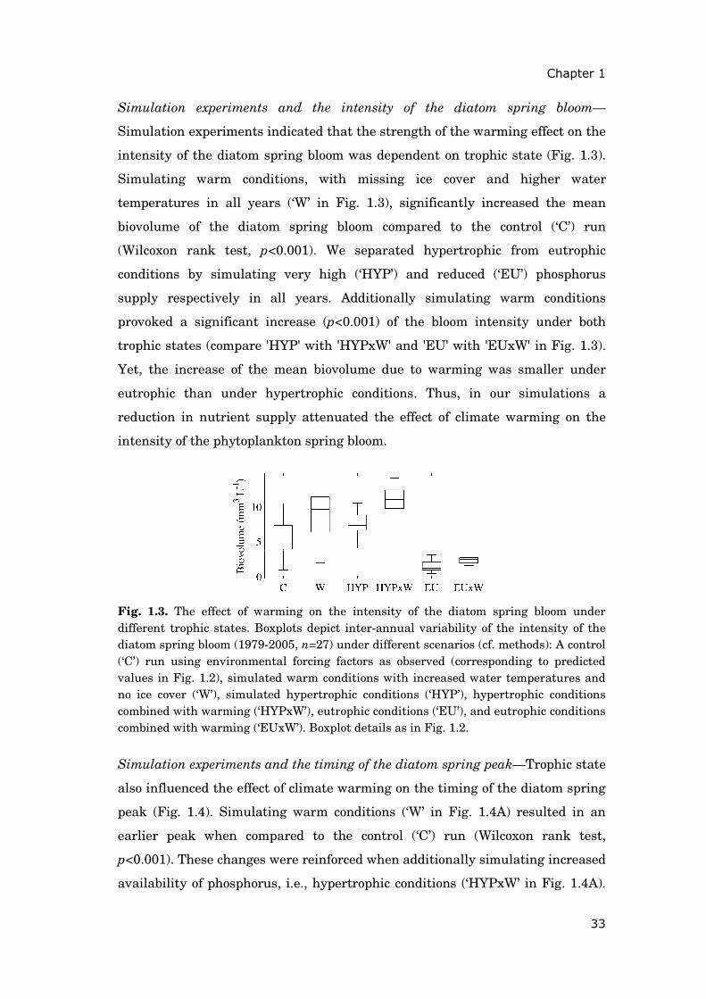
Simulation experiments and the intensity of the diatom spring bloom—

Simulation experiments indicated that the strength of the warming effect on the

intensity of the diatom spring bloom was dependent on trophic state (Fig. 1.3).

Simulating warm conditions, with missing ice cover and higher water

temperatures in all years (‘W’ in Fig. 1.3), significantly increased the mean

biovolume of the diatom spring bloom compared to the control (‘C’) run

(Wilcoxon rank test, p<0.001). We separated hypertrophic from eutrophic

conditions by simulating very high (‘HYP’) and reduced (‘EU’) phosphorus

supply respectively in all years. Additionally simulating warm conditions

provoked a significant increase (p<0.001) of the bloom intensity under both

trophic states (compare 'HYP' with 'HYPxW' and 'EU' with 'EUxW' in Fig. 1.3).

Yet, the increase of the mean biovolume due to warming was smaller under

eutrophic than under hypertrophic conditions. Thus, in our simulations a

reduction in nutrient supply attenuated the effect of climate warming on the

intensity of the phytoplankton spring bloom.

Fig. 1.3. The effect of warming on the intensity of the diatom spring bloom under different trophic states. Boxplots depict inter-annual variability of the intensity of the diatom spring bloom (1979-2005, n=27) under different scenarios (cf. methods): A control (‘C’) run using environmental forcing factors as observed (corresponding to predicted values in Fig. 1.2), simulated warm conditions with increased water temperatures and no ice cover (‘W’), simulated hypertrophic conditions (‘HYP’), hypertrophic conditions combined with warming (‘HYPxW’), eutrophic conditions (‘EU’), and eutrophic conditions combined with warming (‘EUxW’). Boxplot details as in Fig. 1.2.

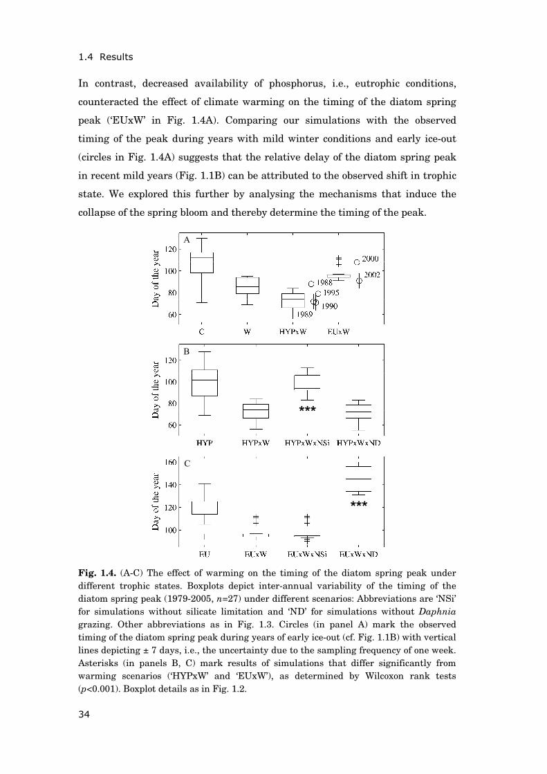
Simulation experiments and the timing of the diatom spring peak—Trophic state

also influenced the effect of climate warming on the timing of the diatom spring

peak (Fig. 1.4). Simulating warm conditions (‘W’ in Fig. 1.4A) resulted in an

earlier peak when compared to the control (‘C’) run (Wilcoxon rank test,

p<0.001). These changes were reinforced when additionally simulating increased

availability of phosphorus, i.e., hypertrophic conditions (‘HYPxW’ in Fig. 1.4A).

1.4 Results

34

In contrast, decreased availability of phosphorus, i.e., eutrophic conditions,

counteracted the effect of climate warming on the timing of the diatom spring

peak (‘EUxW’ in Fig. 1.4A). Comparing our simulations with the observed

timing of the peak during years with mild winter conditions and early ice-out

(circles in Fig. 1.4A) suggests that the relative delay of the diatom spring peak

in recent mild years (Fig. 1.1B) can be attributed to the observed shift in trophic

state. We explored this further by analysing the mechanisms that induce the

collapse of the spring bloom and thereby determine the timing of the peak.

Fig. 1.4. (A-C) The effect of warming on the timing of the diatom spring peak under different trophic states. Boxplots depict inter-annual variability of the timing of the diatom spring peak (1979-2005, n=27) under different scenarios: Abbreviations are ‘NSi’ for simulations without silicate limitation and ‘ND’ for simulations without Daphnia grazing. Other abbreviations as in Fig. 1.3. Circles (in panel A) mark the observed timing of the diatom spring peak during years of early ice-out (cf. Fig. 1.1B) with vertical lines depicting ± 7 days, i.e., the uncertainty due to the sampling frequency of one week. Asterisks (in panels B, C) mark results of simulations that differ significantly from warming scenarios (‘HYPxW’ and ‘EUxW’), as determined by Wilcoxon rank tests (p<0.001). Boxplot details as in Fig. 1.2.

***

***

A

B

C

Chapter 1

35

Bloom collapse mechanisms under different trophic states—Analysing the role of

silicate limitation and Daphnia grazing showed that the mechanisms, which

underlie diatom spring phenology, differ under hypertrophic and eutrophic

conditions (Fig. 1.4B, C). While under hypertrophic conditions (Fig. 1.4B)

neglecting silicate limitation strongly decelerated the warming-induced forward

shift of the peak (‘HYPxW’ vs. ‘HYPxWxNSi’, p<0.001), the effect of warming

persisted when silicate limitation was neglected under eutrophic conditions (Fig.

1.4C, ‘EUxW’ vs. ‘EUxWxNSi’, p>0.1). By contrast, neglecting Daphnia grazing

had hardly any effect on the timing of the peak under simulated hypertrophic

conditions (Fig. 1.4B, ‘HYPxW’ vs. ‘HYPxWxND’, p>0.1), whereas the effect of

warming was annulled and the peak delayed significantly under eutrophic

conditions (Fig. 1.4C, ‘EUxW’ vs. ‘EUxWxND’, p<0.001). Hence, while the

collapse of the bloom was caused by silicate limitation under very high

phosphorus supply (hypertrophic conditions), it was caused by Daphnia grazing

under reduced phosphorus supply (eutrophic conditions).

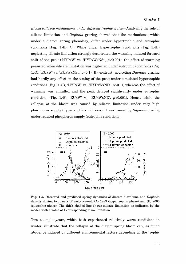
Fig. 1.5. Observed and predicted spring dynamics of diatom biovolume and Daphnia density during two years of early ice-out: (A) 1989 (hypertrophic phase) and (B) 2000 (eutrophic phase). The thick shaded line shows silicate limitation as indicated by the model, with a value of 1 corresponding to no limitation.

Two example years, which both experienced relatively warm conditions in

winter, illustrate that the collapse of the diatom spring bloom can, as found

above, be induced by different environmental factors depending on the trophic

A) 1989 B) 2000

1.5 Discussion

36

state (Fig. 1.5). The model indicates that the diatom spring bloom was

terminated through silicate limitation in 1989 (i.e., in the hypertrophic phase)

as suggested by our simulation experiments (Fig. 1.4B). In contrast, the diatom

spring bloom in 2000 (i.e., in the eutrophic phase) did not collapse until Daphnia

densities became important, again in accordance with our simulation results

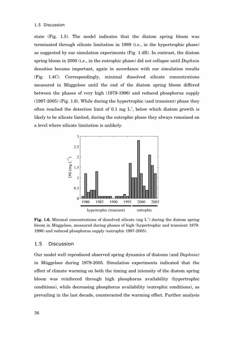
(Fig. 1.4C). Correspondingly, minimal dissolved silicate concentrations

measured in Müggelsee until the end of the diatom spring bloom differed

between the phases of very high (1979-1996) and reduced phosphorus supply

(1997-2005) (Fig. 1.6). While during the hypertrophic (and transient) phase they

often reached the detection limit of 0.1 mg L-1, below which diatom growth is

likely to be silicate limited, during the eutrophic phase they always remained on

a level where silicate limitation is unlikely.

Fig. 1.6. Minimal concentrations of dissolved silicate (mg L-1) during the diatom spring bloom in Müggelsee, measured during phases of high (hypertrophic and transient 1979-1996) and reduced phosphorus supply (eutrophic 1997-2005).

1.5 Discussion

Our model well reproduced observed spring dynamics of diatoms (and Daphnia)

in Müggelsee during 1979-2005. Simulation experiments indicated that the

effect of climate warming on both the timing and intensity of the diatom spring

bloom was reinforced through high phosphorus availability (hypertrophic

conditions), while decreasing phosphorus availability (eutrophic conditions), as

prevailing in the last decade, counteracted the warming effect. Further analysis

hypertrophic (transient) eutrophic

Chapter 1

37

suggested that the collapse of the bloom was caused by silicate limitation during

hypertrophic conditions. In contrast, silicate concentrations did not reach the

limitation threshold during eutrophic conditions such that the bloom was

terminated by Daphnia grazing. This switch in bloom collapse mechanisms

explains why the phytoplankton response to mild winter and spring conditions

differed between the periods of very high and reduced phosphorus loading in the

lake studied here.

Plausibility of bloom collapse mechanisms—Diatom biovolume in Müggelsee is

dominated by small centric species in spring (<30 μm), which belong to the

preferred food size range of Daphnia. In fact, the mean yearly contribution of

centric diatom species to total diatom biovolume until the clear water phase was

65 ± 18 SD % (n=27) in our study period. In addition, larger diatoms such as

Asterionella formosa and Fragilaria crotonensis, also present in Müggelsee, have

been found to be suppressed by Daphnia in other freshwater lakes (Vanni and

Temte 1990). The role of silicate limitation during the diatom spring bloom is

well documented in marine systems (Allen et al. 1998), but has also been shown

to be important in freshwater systems (Lund 1950). Thus, both of our

explanations for the collapse of the diatom bloom are plausible.

The bloom collapse mechanisms proposed here might also contribute to a better

understanding of the effects of climate warming on phytoplankton phenology

described in other studies. Interestingly, in a simulation study by Elliott et al.

(2006), increasing the nutrient (phosphorus and nitrogen) load enhanced the

warming-induced forward shift of the spring peak of the diatom species

Asterionella sp., whereas the timing of the spring peak of the two non-diatom

species Chlorella sp. and Plagioselmis sp. was delayed under increased nutrient

load. This finding is in accordance with our results assuming that in Eliott et

al.’s (2006) simulations increasing phosphorus and nitrogen availability resulted

in higher growth rates of Asterionella sp. and subsequently in an earlier collapse

of the peak caused by silicate limitation. In contrast, Chlorella sp. and

Plagioselmis sp., which were not limited by an additional nutrient, peaked later

in that study because they could fully exploit the larger resource base.

1.5 Discussion

38

Potential food web consequences of a switch in bloom collapse mechanisms—A

bloom collapse induced by silicate limitation, as suggested for mild years during

the hypertrophic phase of Müggelsee (Fig. 1.4B), decouples diatoms from

Daphnia (Fig. 1.5). We wondered whether this decoupling of predator and prey

had any consequences for the growth success of Daphnia. In fact, Winder and

Schindler (2004a) have shown that a climate-induced decoupling of the

phytoplankton bloom from the onset of Daphnia growth in spring can produce a

mismatch situation causing a decline in Daphnia abundance. However, in a

supplementary analysis, we did not find any relationship between the number of

weeks elapsed between the phytoplankton peak and the Daphnia maximum in

spring (as an indicator of the potential mismatch) and Daphnia densities in late

spring and summer (not shown). Moreover, when Daphnia started growing in

spring, the diatom biovolume always stayed above 0.2 mg C L-1 (approximately

1.7 mm3 L-1), which is regarded as the food limitation threshold for Daphnia

(Lampert 1978). Considering that besides diatoms other phytoplankton species

contribute to Daphnia food, it is not surprising that although the phytoplankton

spring peak is decoupled from Daphnia growth in some years, we do not find any

evidence for a mismatch situation between phytoplankton and Daphnia in this

nutrient-rich lake.

Phenomenological approach to phosphorus limitation—A strong correlation

between phytoplankton biomass and total phosphorus concentrations as found

in spring for Müggelsee (Eq. 12) does not necessarily indicate that algal growth

rates are indeed limited by phosphorus (Sommer 1994). Yet, we chose the

phenomenological approach presented here, based on the assumption that

decreasing concentrations of total phosphorus reflect decreasing concentrations

of phosphorus available for algal growth. In fact, previous studies have pointed

to increasingly phosphorus limited phytoplankton spring growth in Müggelsee

(Köhler et al. 2000; Köhler et al. 2005). Such a limitation is plausible, as

concentrations of soluble reactive phosphorus fell below the limitation threshold

of 10 μg L-1 during the phytoplankton spring bloom in all years (Köhler et al.

2005).

Chapter 1

39

When estimating the maximal phosphorus available for diatom growth, we

assumed that a constant amount (TP*=52 μg L-1) is locked in other

compartments (such as bacteria, other phytoplankton species, zooplankton, and

phosphorus bound to iron or calcite) each year (cf. methods). This is a strong

assumption because, intuitively, the amount of phosphorus locked in other

compartments should decrease as total phosphorus concentrations decrease in

the lake. We, therefore, performed two additional regressions (cf. Eq. 12) of

mean spring diatom biovolume (Abloom) on mean spring total phosphorus

concentrations (TPbloom) for the periods 1979-1993 (high TP concentrations) and

1994-2005 (reduced TP concentrations). The estimation of the phosphorus locked

in other compartments was clearly not lower under reduced total phosphorus

concentrations (TP*=56 μg L-1, p<0.001, R2=0.54) than under high total

phosphorus concentrations (TP*=47 μg L-1, p<0.01, R2=0.41). This supports our

assumption that, during the study period, a relatively equal amount of

phosphorus was not available to diatoms independently of trophic state.

Interestingly, a large amount of particulate phosphorus in Müggelsee and its

inflow is bound to iron and not available to phytoplankton growth (Kirchner

1997). Better understanding the phosphorus limitation of phytoplankton in

Müggelsee definitively requires further research, however, the main conclusions

of this study are independent of the exact mechanisms which determine the

intensity of algal biovolume under different trophic states.

Other model simplifications—Model development poses the challenge to find a

balance between including the key processes while keeping the model as simple

as possible. This process necessarily leads to the exclusion of mechanisms that

are known to be important in other systems. For instance, we are aware of the

fact that grazing by copepods and ciliates can be an important loss factor for

phytoplankton early in the year (Huber and Gaedke 2006; Tirok and Gaedke

2006; Peeters et al. 2007a). Yet, a model that included the effect of winter

grazers (based on observed densities and clearance rates from the literature) as

additional forcing factors negligibly improved the fit of the model (not shown).

We also ignored that the maximal uptake rate of phosphorus ρmax can be

dependent on cell quota (Morel 1987). The reason for this was that the

1.5 Discussion

40

regulation of nutrient uptake rates is poorly understood yet (Klausmeier et al.

2004) and modelling the negative feedback of internal nutrient stores on uptake

rates has hardly affected the system behaviour in similar models (Klausmeier et

al. 2004, Diehl unpubl.). Also, studies of phytoplankton physiology have clearly

demonstrated that it is not only the average light availability but day length

that influences phytoplankton growth rates (Nicklisch and Kohl 1989).

Accounting for the latter mechanism would certainly be one of the many steps to

render the model more realistic.

The importance of considering changes in trophic state besides climate

warming—Previous studies on the phytoplankton response to climate warming

in Müggelsee did not find any effect of nutrients (Adrian et al. 1999; Gerten and

Adrian 2000). This might be explained by the shorter time-series used in these

studies ending in the late 90s, when the nutrient effect might not have been

apparent yet. Another explanation could be that, as found here, simple

correlation analysis is not the right tool to detect more subtle relationships as

those between the trophic state and the timing of the phytoplankton spring

bloom. Our results are clearly in accordance with other observational and

modelling studies, showing that the effect of climate warming on the

phytoplankton spring bloom can be counteracted by decreasing nutrient

concentrations (Eliott et al. 2006; Jeppesen et al. 2005). These authors explain

their findings by the well-known positive effect of increasing temperatures and

the negative effect of decreasing nutrient concentrations on phytoplankton

growth (Wernicke and Nicklisch 1986). Here, we show that decreasing

phosphorus concentrations do not only imply a gradual shift of increasingly

phosphorus-limited algal growth, but a qualitative switch from a bottom-up

driven (by silicate limitation) to a top-down controlled (by Daphnia grazing)

collapse of the phytoplankton spring bloom.

The interaction between climate warming and a change in nutrient loading can

be expected to occur in other aquatic ecosystems of different trophic state (such

as meso- or oligotrophic lakes) and of different types (such as deep lakes or

marine systems). The mechanisms underlying this interaction might differ

between the ecosystems. However, there are some indications that the switch in

Chapter 1

41

bloom collapse mechanisms that we propose here for the shallow, heavily loaded

lake might also be relevant for other systems. Schelske and Stoermer (1971)

first postulated a relationship between eutrophication and the increasing

occurrence of silicate limitation of diatom growth for the deep, oligotrophic Lake

Michigan. This relationship has also been described for marine systems, such as

the heavily loaded, mesohaline part of Chesapeake Bay and for coastal waters of

the North Sea (Conley et al. 1993). Thus, it is conceivable that a switch from an

algal bloom collapse induced or at least accelerated by silicate limitation to a

collapse induced by some other factor (such as grazing or sedimentation) takes

place in the course of a load reduction in these systems as well. Simultaneous

climate warming should then amplify the changes brought about by a shift in

trophic state just as it has been found in this study.

1.6 Conclusions

In conclusion, other studies have pointed to the risk of falsely attributing

observed changes in aquatic ecosystems to climate warming (Jeppesen et al.

2003; Van Donk et al. 2003; Jeppesen et al. 2005). Here, we emphasize the

necessity of gaining a better understanding of the mechanisms that underlie

phenology shifts and other climate-induced changes in aquatic ecosystems. For

instance, it has become increasingly clear that the mechanisms determining the

phytoplankton response to climate warming differ strongly between shallow and

deep lakes (Adrian et al. 1999; Peeters et al. 2007a). Our results show that it is

equally important to consider the trophic state of a lake when investigating the

mechanisms underlying the effect of global warming on phytoplankton bloom

formation. In view of future climate warming, further studies are needed to

determine how climatic conditions influence the external and internal nutrient

loading of lakes (e.g., Malmaeus et al. 2006). Moreover, other anthropogenic

interventions (such as land use and management changes), which influence the

nutrient supply to lakes and rivers, have to be taken into account in order to

establish more realistic scenarios of freshwater ecosystems under anticipated

climate change.

1.7 Acknowledgements

42

1.7 Acknowledgements

We thank Sebastian Diehl for his helpful comments during the model

construction process and on the method section of the manuscript, Ursula

Gaedke for advising us on many model related questions, Andreas Nicklisch and

Jan Köhler for their advice on phytoplankton dynamics in Müggelsee and all

scientists and technicians involved in the collection and compilation of the long-

term data set. We are also grateful to Don Scavia and one anonymous referee for

giving valuable comments on the first version of the manuscript. The German

Research Foundation (DFG) supported Veronika Huber within the program

AQUASHIFT (SPP 1162).

Chapter 1

1.8 Appendix

Genetic algorithm—A genetic algorithm is a computational search technique

inspired by evolutionary biology that allows approximating solutions to

optimization problems. Here, the aim is to find a parameter set that optimizes

the fit between the (sub-) model and the data. The genetic algorithm comprises

four major building blocks: the initialization of parameter sets (the creation of

the initial ‘population’), the selection of the best parameter sets based on model

performance (selection based on ‘fitness’), the recombination of the selected

parameter sets (‘crossover’), and randomly altering parameter values

(‘mutation’). In this study, the sequence of selection, crossover, and mutation

was repeated for 1000 generations. After the last generation, one final selection

procedure was run and the parameter set with the best performance (the

highest fitness) provided the default parameter values (cf. Table 1.1) for the

subsequent model analysis.

We separately calibrated, first, the Daphnia sub-model and, second, the diatom

core model. In the following, we describe the design of the genetic algorithm for

the diatom core model and then mention a few changes specific to the Daphnia

sub-model.

Creation of an initial population—The genetic algorithm was initialized by

creating a suit of 36 parameter sets, which proved to be sufficient for our

calibration problem. Each parameter set consisted of 8 calibration parameters

that were drawn randomly from the biologically plausible intervals given in

Table 1.1.

Selection based on fitness—The differential equations (Eqs. 1-4) were solved for

each of the 36 parameter sets created during the initialization process (using the

solution for Daphnia density from Eqs. 13-15 as a forcing variable). For each

solution, the fit between the model and the data was assessed by calculating the

weighted mean absolute deviation between predicted (pBi) and observed (oBi)

diatom biovolumes (modified from Willmott 1982)

1.8 Appendix

44

y

n

k k

n

iiii

b nn

oBoBpB

MAD

y

k

∑∑

=

=

−

= 1

1

(A1)

where ny is the number of years in the calibration period, and nk are the different

numbers of observations during each year. The algorithm also calculated the

mean absolute deviation between predicted (pTi) and observed (oTi) timing of the

diatom spring peak.

y

n

kkk

t n

oTpTMAD

y

∑=

−= 1 (A2)

The performance of a parameter set (the fitness F of an individual) was defined

as

b

B

t

T

MADw

MADwF += (A3)

where wT and wB are weighting factors that we chose to set to 1 and 5

respectively. The choice of the weighting factor required several trial runs of the

calibration algorithm, examining the distributions of MADt and MADb, and

adjusting the weighting factors until a satisfactory, qualitative fit of the model

to the data was reached. Once the performance of each parameter set was

evaluated, a total of 6 parameter sets were selected: the two sets that produced

the highest fitness, and four other parameter sets randomly with a probability

proportional to their fitness F.

Crossover—A new suit of parameter sets was constructed by keeping the 6

parameter sets chosen in the selection procedure and by recombining all possible

pairs of these parameter sets (producing 30 new additional parameter sets). The

recombination imitates the chromosomal crossover with each parameter set

representing a string of genes. It consisted of cutting the parameter string of two

sets at a random position and creating two new sets by combining the

corresponding parts of the parameter strings.

Mutation—Random changes were imposed on all new parameter sets except for

the parameter set that produced the best model performance. Each parameter

Chapter 1

45

‘mutated’ with a probability of 0.4 by adding (deducting) a value drawn

randomly from the mutation range, which is half of the corresponding biological

plausible parameter interval. If the new parameter value lay outside the given

parameter interval, the parameter was set to the maximal (minimal) allowed

value.

Calibrating the Daphnia sub-model—Since the Daphnia sub-model required the

calibration of fewer parameters, it was sufficient to run the genetic algorithm

with a suit of 16 parameter sets, choosing 4 during each selection procedure. The

fitness function consisted of the sum of the indices of agreement IoAt and IoAb (as

described in the method section of the manuscript) and of the reciprocals of

MADt and MADb.

46

Chapter 2

Periodically forced food chain dynamics: model predictions and experimental validation

______________________________

Published as Steiner C.F., A.S. Schwaderer, V. Huber, C.A. Klausmeier and E. Litchman (2009) Periodically forced food chain dynamics: model predictions and

experimental validation. Ecology, 90, 3099-3107.

2.1 Abstract

48

2.1 Abstract

Despite the recognition of the importance of seasonal forcing in nature,

remarkably few studies have theoretically explored periodically forced

community dynamics. Here we employ a novel approach called “successional

state dynamics” (SSD) to model a seasonally forced predator-prey system. We

first generated analytical predictions of the effects of altered seasonality on

species persistence and the timing of community state transitions. We then

parameterized the model using a zooplankton-phytoplankton system and tested

quantitative predictions using controlled experiments. In the majority of cases,

timing of zooplankton and algal population peaks matched model predictions.

Decreases in growing period length delayed algal blooms, consequently delaying

peaks in zooplankton abundance. Predictions of increased probability of

predator extinction at low growing period lengths were also upheld

experimentally. Our results highlight the utility of the SSD modeling approach

as a framework for predicting the effects of altered seasonality on the structure

and dynamics of multitrophic communities.

Chapter 2

49

2.2 Introduction

Approaches to modeling consumer-resource interactions have frequently relied

on the assumption that systems are at equilibrium and that parameters

governing species vital rates are fixed through time. While such approaches

have proven powerful in identifying key ecological mechanisms and processes,

most ecologists recognize that many natural systems experience temporally

varying environmental conditions that can buffet populations, enhance

background mortality rates, and drive population trajectories far from steady-

state conditions. Hence, perceived patterns of community structure may actually

be in flux as populations are frequently within transitory phases due to external

forcing (Hastings 2001, 2004; Jäger et al. 2008). The overriding influence of

temporal heterogeneity on community dynamics is most readily apparent in

temperate and high latitude systems in which seasonal variation imposes

periods of active somatic and population growth followed by periods of depressed

metabolic activity, dormancy and increased mortality. Predicting the long-term

consequences of such periodic forcing on the dynamics and structure of

communities is a challenge to ecologists and may prove especially vital in the

near future as large-scale climate change threatens to alter the strength and

timing of seasonality in many natural systems (Walther et al. 2002; Parmesan

and Yohe 2003).

Despite the recognition of the importance of temporal variability and seasonal

forcing in nature, remarkably few studies have theoretically explored how

periodic mortality events alter community dynamics within spatially

homogeneous, closed systems (though see Scheffer et al. 1997; Ives et al. 2000).

One obstacle towards theoretical advancement is the lack of analytical

techniques for exploring the effects of large perturbations with long period

lengths. Recently, Klausmeier (unpublished manuscript) outlined a general

methodology for theoretically examining the effects of seasonal mortality events

on community dynamics, based on earlier work (Litchman and Klausmeier

2001). Called “successional state dynamics” (SSD), the model framework treats

compositional succession of a community as a path taken through different

community equilibria during an active growing period which is periodically reset

2.2 Introduction

50

to a near empty state during a period of intensified mortality (e.g., the winter

season).

Here we employ the SSD approach to model the dynamics of a periodically

forced food chain composed of a single top predator and a single prey. We

generate quantitative predictions of the effects of growing season length on the

timing of key state transitions of the system using a simple planktonic system

as a model basis. We then test these predictions using controlled laboratory

experiments. Planktonic communities are excellent model systems for

examining the impacts of seasonal forcing on community dynamics as they are

known to exhibit repeatable patterns of seasonal succession in nature (Sommer

et al. 1986; Sommer 1989). Moreover, alterations in seasonality and growing

season length are believed to have strong effects on zooplankton-algal dynamics

and the timing of key events such as spring algal blooms, peaks in zooplankton

abundance, and the clear water phase (Straile and Adrian 2000; Straile 2002;

Mooij et al. 2005; Berger et al. 2007; Huber et al. 2008). Hence, model

development and experimental validation using simplified modules of these

systems are important first steps towards understanding natural variation in

seasonal patterns.

Model predictions—In-depth analysis of the effects of periodic forcing on

community dynamics using the SSD approach will be presented in a future

paper (Klausmeier unpublished manuscript). Here we outline the salient

features and predictions of the SSD food chain model. The SSD approach models

seasonal succession as a path through possible community equilibria (or

“states”) of the non-forced system. In a system composed of a single zooplankton

predator (Z) and its phytoplankton prey (P), there are three possible community

states: prey present and predator absent, predator and prey both present, and

the empty state (both predator and prey absent). Given these possible states,

there are only two nontrivial successional trajectories the system may take

following winter mortality: 1) the empty state to prey present and 2) the empty

state to prey present to a state with both predator and prey present. The SSD

model assumes that changes in log transformed predator and prey densities

approach a linear form over time (Fig. 2.1A).

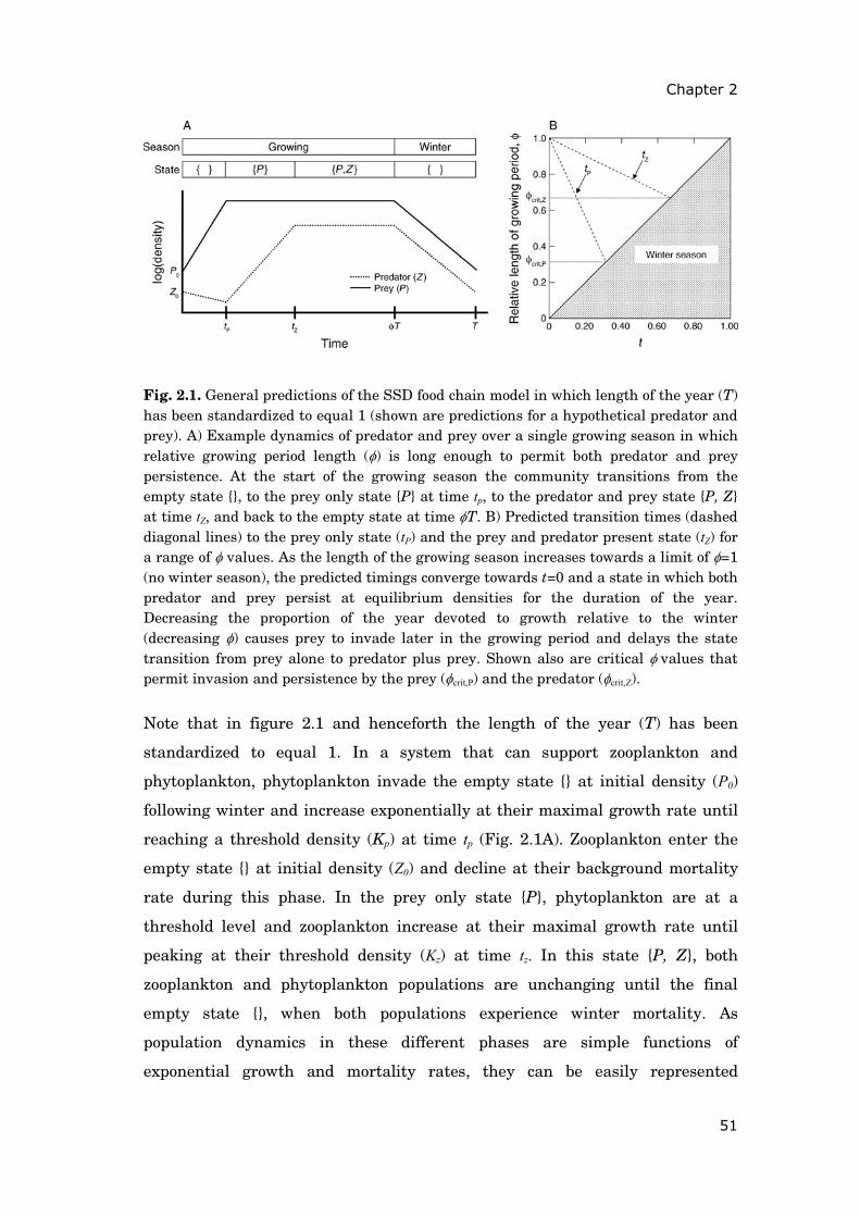
Chapter 2

51

Fig. 2.1. General predictions of the SSD food chain model in which length of the year (T) has been standardized to equal 1 (shown are predictions for a hypothetical predator and prey). A) Example dynamics of predator and prey over a single growing season in which relative growing period length (φ) is long enough to permit both predator and prey persistence. At the start of the growing season the community transitions from the empty state {}, to the prey only state {P} at time tp, to the predator and prey state {P, Z} at time tZ, and back to the empty state at time φT. B) Predicted transition times (dashed diagonal lines) to the prey only state (tP) and the prey and predator present state (tZ) for a range of φ values. As the length of the growing season increases towards a limit of φ=1 (no winter season), the predicted timings converge towards t=0 and a state in which both predator and prey persist at equilibrium densities for the duration of the year. Decreasing the proportion of the year devoted to growth relative to the winter (decreasing φ) causes prey to invade later in the growing period and delays the state transition from prey alone to predator plus prey. Shown also are critical φ values that permit invasion and persistence by the prey (φcrit,P) and the predator (φcrit,Z).

Note that in figure 2.1 and henceforth the length of the year (T) has been

standardized to equal 1. In a system that can support zooplankton and

phytoplankton, phytoplankton invade the empty state {} at initial density (P0)

following winter and increase exponentially at their maximal growth rate until

reaching a threshold density (Kp) at time tp (Fig. 2.1A). Zooplankton enter the

empty state {} at initial density (Z0) and decline at their background mortality

rate during this phase. In the prey only state {P}, phytoplankton are at a

threshold level and zooplankton increase at their maximal growth rate until

peaking at their threshold density (Kz) at time tz. In this state {P, Z}, both

zooplankton and phytoplankton populations are unchanging until the final

empty state {}, when both populations experience winter mortality. As

population dynamics in these different phases are simple functions of

exponential growth and mortality rates, they can be easily represented

2.2 Introduction

52

mathematically. The long term population growth rate of phytoplankton (ΛP)

averaged over a period is:

(1)

where λP,{},growing is its growth rate when invading the empty state early in the

growing season, tp is the proportion of the year required for phytoplankton to

reach equilibrium when invading (after which net growth rate equals zero), and

λP,{},winter is its mortality rate during the winter season weighted by the proportion

of the year that is winter (1-φ). For the invading predator (Z), long term growth

averaged over a period is:

(2)

where λZ,{},winter is the predator’s winter mortality rate, λZ,{},growing is its growth rate

when invading the empty state (which is assumed to be negative and equal to its

background mortality) and λZ,{P},growing is its exponential growth rate following

successful prey invasion (at time tp) which proceeds until the predator reaches

an equilibrium density at time tz.

Model predictions of the effects of relative length of the growing period (φ) on the

timing of state transitions can be easily ascertained by assuming that the

system has settled to a stable seasonal trajectory, setting equations 1 and 2 to

zero and solving for tp and tz (Klausmeier unpublished manuscript). Doing so

produces the following relationships:

(3)

(4)

Furthermore, critical φ values that permit successful invasion of predator and

prey can also be determined. The minimum φ permitting invasion and

persistence by the prey (φcrit,P) is found by setting φcrit,P=φ=tp and solving equation

3. Similarly, the minimum φ permitting predator invasion (φcrit,Z) is found by

{ } { } )1(λλ winter,P,growing,P, φ−+=Λ PP t

{ } { } { } )1(λ)(λλ winter,Z,growing,PZ,growing,Z, φ−+−+=Λ PZPZ ttt

{ } { } { }

{ } growing,PZ,

winter,Z,growing,PZ,growing,Z,

λ

)1(λλλ φ−−+−=

PPZ

ttt

{ }

{ } growing,P,

winter,P,

λ)1(λ φ−−

=Pt

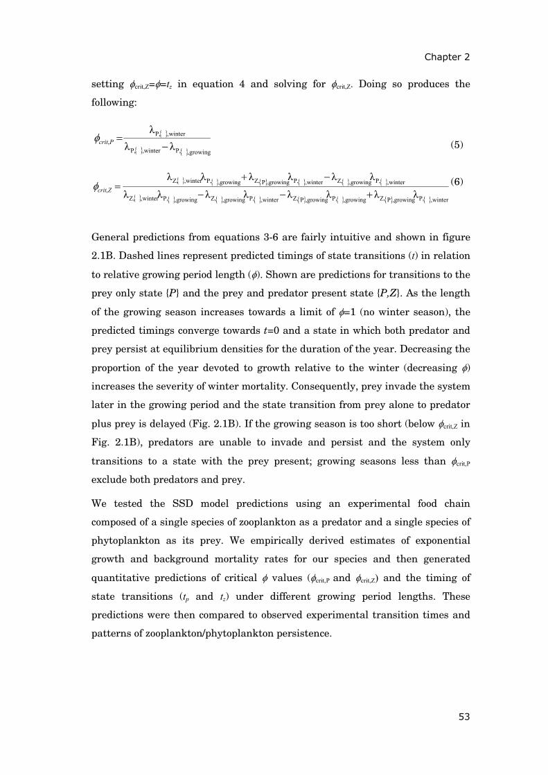
Chapter 2

53

setting φcrit,Z=φ=tz in equation 4 and solving for φcrit,Z. Doing so produces the

following:

(5)

(6)

General predictions from equations 3-6 are fairly intuitive and shown in figure

2.1B. Dashed lines represent predicted timings of state transitions (t) in relation

to relative growing period length (φ). Shown are predictions for transitions to the

prey only state {P} and the prey and predator present state {P,Z}. As the length

of the growing season increases towards a limit of φ=1 (no winter season), the

predicted timings converge towards t=0 and a state in which both predator and

prey persist at equilibrium densities for the duration of the year. Decreasing the

proportion of the year devoted to growth relative to the winter (decreasing φ)

increases the severity of winter mortality. Consequently, prey invade the system

later in the growing period and the state transition from prey alone to predator

plus prey is delayed (Fig. 2.1B). If the growing season is too short (below φcrit,Z in

Fig. 2.1B), predators are unable to invade and persist and the system only

transitions to a state with the prey present; growing seasons less than φcrit,P

exclude both predators and prey.

We tested the SSD model predictions using an experimental food chain

composed of a single species of zooplankton as a predator and a single species of

phytoplankton as its prey. We empirically derived estimates of exponential

growth and background mortality rates for our species and then generated

quantitative predictions of critical φ values (φcrit,P and φcrit,Z) and the timing of

state transitions (tp and tz) under different growing period lengths. These

predictions were then compared to observed experimental transition times and

patterns of zooplankton/phytoplankton persistence.

{ }

{ } { } growing,P,winter,P,

winter,P,, λλ

λ−

=Pcritφ

{ } { } { } { } { } { }

{ } { } { } { } { } { } { } { } winter,P,growing,PZ,growing,P,growing,PZ,winter,P,growing,Z,growing,P,winter,Z,

winter,P,growing,Z,winter,P,growing,PZ,growing,P,winter,Z,, λλλλλλλλ

λλλλλλ

+−−

−+=Zcritφ

2.3 Methods

54

2.3 Methods

Experimental system—Experiments were conducted using a laboratory-based

system consisting of the rotifer Brachionus calyciflorus as a predator and the

flagellated green alga Chlamydomonas reinhardtii as its prey (all species are

hereafter referred to by genus). We obtained Brachionus cultures from Florida

Aqua Farms (Dade City, FL, USA), while Chlamydomonas was a wild type

strain (#CC-2935) obtained from the Chlamydomonas Genetics Center (Duke

University, Durham, NC, USA). Brachionus cultures were fed the same

Chlamydomonas strain used in the experiment and all stock cultures were

maintained using the same medium and environmental conditions as in the

experiment. Experimental vessels consisted of 1000mL flasks loosely capped

with aluminum foil and filled with 800mL of COMBO medium; medium was

prepared as in Kilham et al. (1998) except that phosphorus was added at a

lowered concentration of 490 μg/L to minimize formation of non-motile algal

cells (Harris 1989). All flasks were housed and randomly ordered in a single

environmental chamber at 25oC under 24 hour light; flasks were rotated on the

chamber shelves daily. During the experiment, flasks were manually mixed and

had 10% of their volume removed and replaced with fresh medium once daily

(removed medium served as a zooplankton and phytoplankton sample). Both

Brachionus and Chlamydomonas are motile and found in the water column;

manual mixing helped ensure that nutrients and organisms remained relatively

homogenous in their distributions. Brachionus were enumerated using a

dissecting scope while Chlamydomonas were counted using a CASY particle

counter. As Brachionus males do not actively feed and were rare, population

densities of Brachionus were based only on counts of females. All experimental

materials were autoclave-sterilized prior to use.

We tested the capacity of our model to predict the timing of state transitions for

different relative growing period lengths. Experimentally, the proportion of the

year devoted to the growing period (φ) versus winter can be easily manipulated

by periodically imposing different levels of winter mortality via a single, large-

scale mortality event. For example, an imposed mortality event of 90% of the

community would correspond to a longer winter period compared to a mortality

event with 50% removal. We employed five relative growing period treatments:

Chapter 2

55

φ = 0.65, 0.70, 0.75, 0.80, and 0.85, with each treatment replicated four times.

Our previous pilot experiments and model simulations showed that Brachionus

and Chlamydomonas could persist at these φ levels and that the φ=0.65

treatment was close to the critical φ (φcrit,Z) for Brachionus, allowing us to test the

effects of decreased φ on the probability of predator extinction. To

experimentally impose winter mortality, a percentage of the community was

removed by volume from each flask, added to a new flask and then brought to

800mL total with fresh, sterile medium. Percentage of volume D removed for

each treatment was calculated using { } 100)')1(λexp( winter, ⋅−= TD φ , where

λ{},winter is the winter mortality rate for both predator and prey arbitrarily set to -1

day-1, and T’ is the absolute length of the full period (growing season plus

winter). T’ can be easily calculated from max' tT =φ where tmax is the time the

organisms where allowed to grow between mortality events (set to 14 days for all

treatments). A fourteen day growing length was chosen based on preliminary

experiments which showed that Brachionus densities peaked and equilibrated

by day 14.

At the start of the experiment, 20 cells/mL of Chlamydomonas were added to all

experimental flasks. Algae were allowed to reproduce for seven days at which

time Brachionus individuals were haphazardly isolated from stock cultures and

added at a density of 0.125 individuals/mL. Zooplankton were allowed to

reproduce for 14 days, reaching a peak in density; we refer to this initial growth

period as “year 0”. On day 14, the first winter mortality event was imposed and

communities were allowed to numerically respond for 14 days; we refer to this

growth period as “year 1”. A second winter mortality was then imposed and

communities were again allowed to respond for another 14 days (“year 2”) at

which time the experiment was terminated.

Quantitative predictions and data analysis—To generate quantitative

predictions of the timing of state transitions for our treatments, we

parameterized our model using data from year 1 of the experiment. Estimates of

species growth rates, background mortality rates (λ’s), initial densities (P0 and

Z0) and threshold densities (Kp and Kz) were obtained by fitting the log-linear

2.3 Methods

56

SSD model structure (as in Fig. 2.1A) simultaneously to ln transformed

Brachionus and Chlamydomonas densities using a genetic algorithm (Haupt

and Haupt 1998). Unlike conventional parametric model fitting, we employed a

rule-based approach to obtain the SSD model fits. Fitting the SSD model

structure translates to parameterizing rules that are used to numerically project

the community forward in time as in Fig. 2.1A (Klausmeier unpublished

manuscript). These rules dictate λ’s based on the state of the system and

determine how state transitions occur in the system. Specifically, populations

grow or shrink exponentially at rates determined by the current state of the

system (i.e., which species are at their threshold abundances). Transitions take

place when a population is projected to reach its threshold abundance or when

winter occurs. The procedure consisted of repeating the following steps: 1) time

increments to all potential state transitions are calculated; 2) the temporally

closest transition is chosen to occur; and 3) population densities and the state of

the system are updated accordingly (Klausmeier unpublished manuscript).

While conventional gradient search methods are not appropriate for this type of

rule-based model parameterization, other optimization techniques such as

genetic algorithms can easily handle these problems. For details on the genetic

algorithm procedure used see Appendix B. Models were fit to data from each

treatment replicate separately. After obtaining λ estimates for each replicate

from the model fits, critical φ values (φcrit,P and φcrit,Z) were calculated by solving

equations 5 and 6 for all possible combinations of λ’s (n = 20 for φcrit,P, and n = 203

for φcrit,Z). Similarly, we calculated transition times (tp and tz) based on all

combinations of λ’s (equations 3 and 4) for all treatment level φ values (φ = 0.65,

0.7, 0.75, 0.8, and 0.85). Predictions for mean critical φ values and transition

times were determined by calculating the mean (and standard deviations) of the

resultant distributions.

Model predictions generated from our year 1 model fits were compared to

observed transition times from year 2 of the experiment. To estimate transition

times in year 2, we again fit the SSD log-linear model to ln transformed year 2

data for each replicate separately using the genetic algorithm (as for year 1).

This yielded estimates for initial densities (P0 and Z0), threshold densities (Kp

and Kz) and vital rates (λ’s) for each replicate. Instead of calculating transition

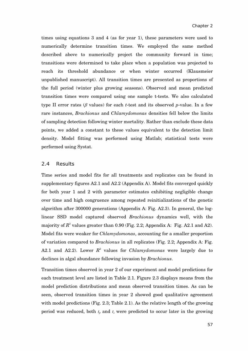
Chapter 2

57

times using equations 3 and 4 (as for year 1), these parameters were used to

numerically determine transition times. We employed the same method

described above to numerically project the community forward in time;

transitions were determined to take place when a population was projected to

reach its threshold abundance or when winter occurred (Klausmeier

unpublished manuscript). All transition times are presented as proportions of

the full period (winter plus growing seasons). Observed and mean predicted

transition times were compared using one sample t-tests. We also calculated

type II error rates (β values) for each t-test and its observed p-value. In a few

rare instances, Brachionus and Chlamydomonas densities fell below the limits

of sampling detection following winter mortality. Rather than exclude these data

points, we added a constant to these values equivalent to the detection limit

density. Model fitting was performed using Matlab; statistical tests were

performed using Systat.

2.4 Results

Time series and model fits for all treatments and replicates can be found in

supplementary figures A2.1 and A2.2 (Appendix A). Model fits converged quickly

for both year 1 and 2 with parameter estimates exhibiting negligible change

over time and high congruence among repeated reinitializations of the genetic

algorithm after 300000 generations (Appendix A: Fig. A2.3). In general, the log-

linear SSD model captured observed Brachionus dynamics well, with the

majority of R2 values greater than 0.90 (Fig. 2.2; Appendix A: Fig. A2.1 and A2).

Model fits were weaker for Chlamydomonas, accounting for a smaller proportion

of variation compared to Brachionus in all replicates (Fig. 2.2; Appendix A: Fig.

A2.1 and A2.2). Lower R2 values for Chlamydomonas were largely due to

declines in algal abundance following invasion by Brachionus.

Transition times observed in year 2 of our experiment and model predictions for

each treatment level are listed in Table 2.1. Figure 2.3 displays means from the

model prediction distributions and mean observed transition times. As can be

seen, observed transition times in year 2 showed good qualitative agreement

with model predictions (Fig. 2.3; Table 2.1). As the relative length of the growing

period was reduced, both tp and tz were predicted to occur later in the growing

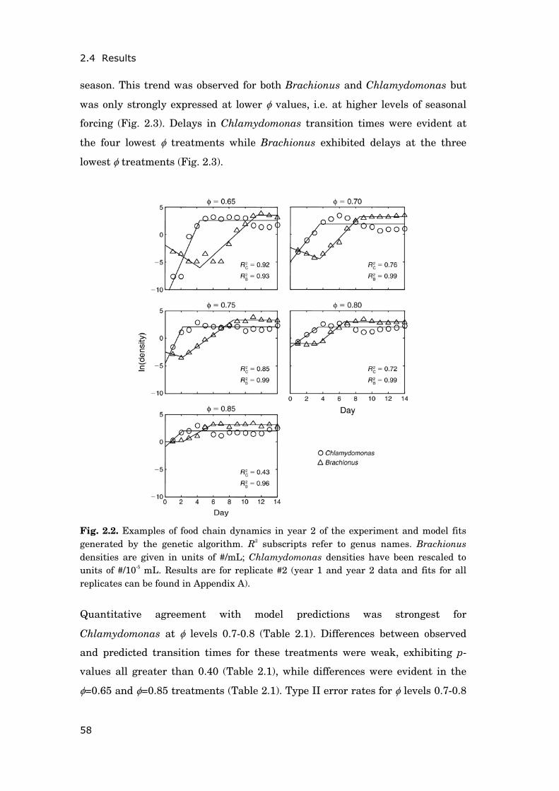
2.4 Results

58

season. This trend was observed for both Brachionus and Chlamydomonas but

was only strongly expressed at lower φ values, i.e. at higher levels of seasonal

forcing (Fig. 2.3). Delays in Chlamydomonas transition times were evident at

the four lowest φ treatments while Brachionus exhibited delays at the three

lowest φ treatments (Fig. 2.3).

Fig. 2.2. Examples of food chain dynamics in year 2 of the experiment and model fits generated by the genetic algorithm. R2 subscripts refer to genus names. Brachionus densities are given in units of #/mL; Chlamydomonas densities have been rescaled to units of #/10-5 mL. Results are for replicate #2 (year 1 and year 2 data and fits for all replicates can be found in Appendix A).

Quantitative agreement with model predictions was strongest for

Chlamydomonas at φ levels 0.7-0.8 (Table 2.1). Differences between observed

and predicted transition times for these treatments were weak, exhibiting p-

values all greater than 0.40 (Table 2.1), while differences were evident in the

φ=0.65 and φ=0.85 treatments (Table 2.1). Type II error rates for φ levels 0.7-0.8

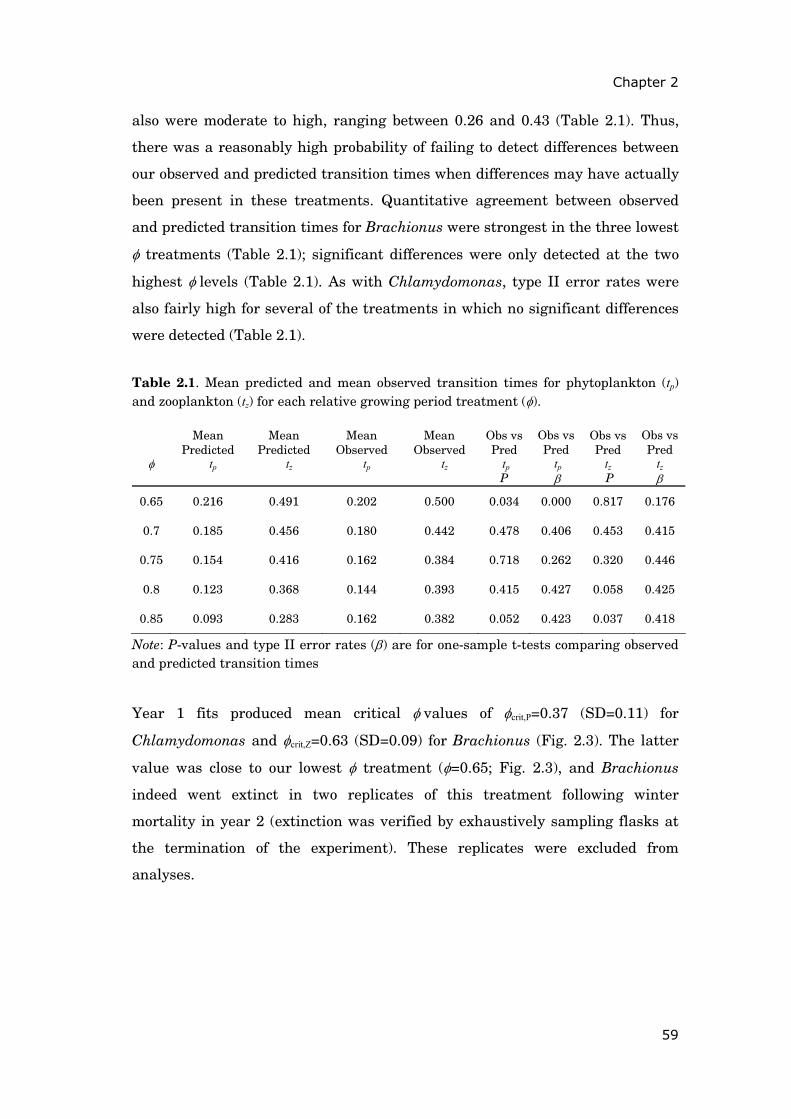
Chapter 2

59

also were moderate to high, ranging between 0.26 and 0.43 (Table 2.1). Thus,

there was a reasonably high probability of failing to detect differences between

our observed and predicted transition times when differences may have actually

been present in these treatments. Quantitative agreement between observed

and predicted transition times for Brachionus were strongest in the three lowest

φ treatments (Table 2.1); significant differences were only detected at the two

highest φ levels (Table 2.1). As with Chlamydomonas, type II error rates were

also fairly high for several of the treatments in which no significant differences

were detected (Table 2.1).

Table 2.1. Mean predicted and mean observed transition times for phytoplankton (tp) and zooplankton (tz) for each relative growing period treatment (φ).

φ

Mean Predicted

tp

Mean Predicted

tz

Mean Observed

tp

Mean Observed

tz

Obs vs Pred

tp P

Obs vs Pred

tp β

Obs vs Pred

tz P

Obs vs Pred

tz β

0.65 0.216 0.491 0.202 0.500 0.034 0.000 0.817 0.176

0.7 0.185 0.456 0.180 0.442 0.478 0.406 0.453 0.415

0.75 0.154 0.416 0.162 0.384 0.718 0.262 0.320 0.446

0.8 0.123 0.368 0.144 0.393 0.415 0.427 0.058 0.425

0.85 0.093 0.283 0.162 0.382 0.052 0.423 0.037 0.418

Note: P-values and type II error rates (β) are for one-sample t-tests comparing observed and predicted transition times

Year 1 fits produced mean critical φ values of φcrit,P=0.37 (SD=0.11) for

Chlamydomonas and φcrit,Z=0.63 (SD=0.09) for Brachionus (Fig. 2.3). The latter

value was close to our lowest φ treatment (φ=0.65; Fig. 2.3), and Brachionus

indeed went extinct in two replicates of this treatment following winter

mortality in year 2 (extinction was verified by exhaustively sampling flasks at

the termination of the experiment). These replicates were excluded from

analyses.

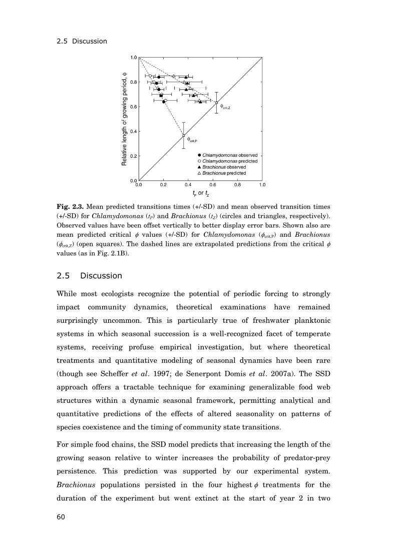
2.5 Discussion

60

Fig. 2.3. Mean predicted transitions times (+/-SD) and mean observed transition times (+/-SD) for Chlamydomonas (tP) and Brachionus (tZ) (circles and triangles, respectively). Observed values have been offset vertically to better display error bars. Shown also are mean predicted critical φ values (+/-SD) for Chlamydomonas (φcrit,P) and Brachionus (φcrit,Z) (open squares). The dashed lines are extrapolated predictions from the critical φ values (as in Fig. 2.1B).

2.5 Discussion

While most ecologists recognize the potential of periodic forcing to strongly

impact community dynamics, theoretical examinations have remained

surprisingly uncommon. This is particularly true of freshwater planktonic

systems in which seasonal succession is a well-recognized facet of temperate

systems, receiving profuse empirical investigation, but where theoretical

treatments and quantitative modeling of seasonal dynamics have been rare

(though see Scheffer et al. 1997; de Senerpont Domis et al. 2007a). The SSD

approach offers a tractable technique for examining generalizable food web

structures within a dynamic seasonal framework, permitting analytical and

quantitative predictions of the effects of altered seasonality on patterns of

species coexistence and the timing of community state transitions.

For simple food chains, the SSD model predicts that increasing the length of the

growing season relative to winter increases the probability of predator-prey

persistence. This prediction was supported by our experimental system.

Brachionus populations persisted in the four highest φ treatments for the

duration of the experiment but went extinct at the start of year 2 in two

Chapter 2

61

replicates of the φ=0.65 treatment – the treatment with the shortest relative

growing period and most severe winter mortality. This treatment level was very

close to the critical φ for Brachionus predicted by our model (φcrit,Z=0.63) below

which extinction is expected.

In addition to facilitating predator/prey persistence, increasing growing period

length relative to winter was predicted to hasten invasion by both predator and

prey during the active growing season. Thus, transition times (tp and tz) were

expected to occur earlier in the year with increasing levels of φ. This prediction

is consistent with long-term patterns of zooplankton-algal dynamics in natural

systems in which warming trends have advanced seasonal community

development (e.g., Straile 2002). Our experiment provided further evidence of

shifts in successional dynamics with altered seasonality; both Chlamydomonas

and Brachionus exhibited accelerated transitions times with increasing φ,

although effects of extended growing seasons on zooplankton-algal peaks were

more strongly expressed in the lower φ treatments. For both Chlamydomonas

and Brachionus, observed transition times tended to occur later than predicted

at the two highest period lengths (φ=0.80 and 0.85).

Deviations between observed and predicted timings could be due to several

factors. First, a key assumption when generating our model predictions was that

the system had settled onto a stable seasonal trajectory. This assumes that

species’ initial densities at the start of the growing season are unchanging from

year to year. However, it was possible that two rounds of winter mortality were

insufficient to attain stability in our experimental system. When comparing

Chlamydomonas initial densities obtained from our model fits for each replicate,

we found no differences between years (Appendix A: Fig. A2.4). However,

Brachionus showed evidence of lower initial densities in year 2 compared to year

1 with differences being strongest in the three highest φ treatments (Appendix

A: Fig. A2.4). Low densities early in the growing period should translate into

delayed peaks in abundance later in the growing period potentially explaining tz

values higher than predicted.

Another assumption of our model was that species’ vital rates (λ) were constant

across φ treatments and across years. This assumption was not upheld in our

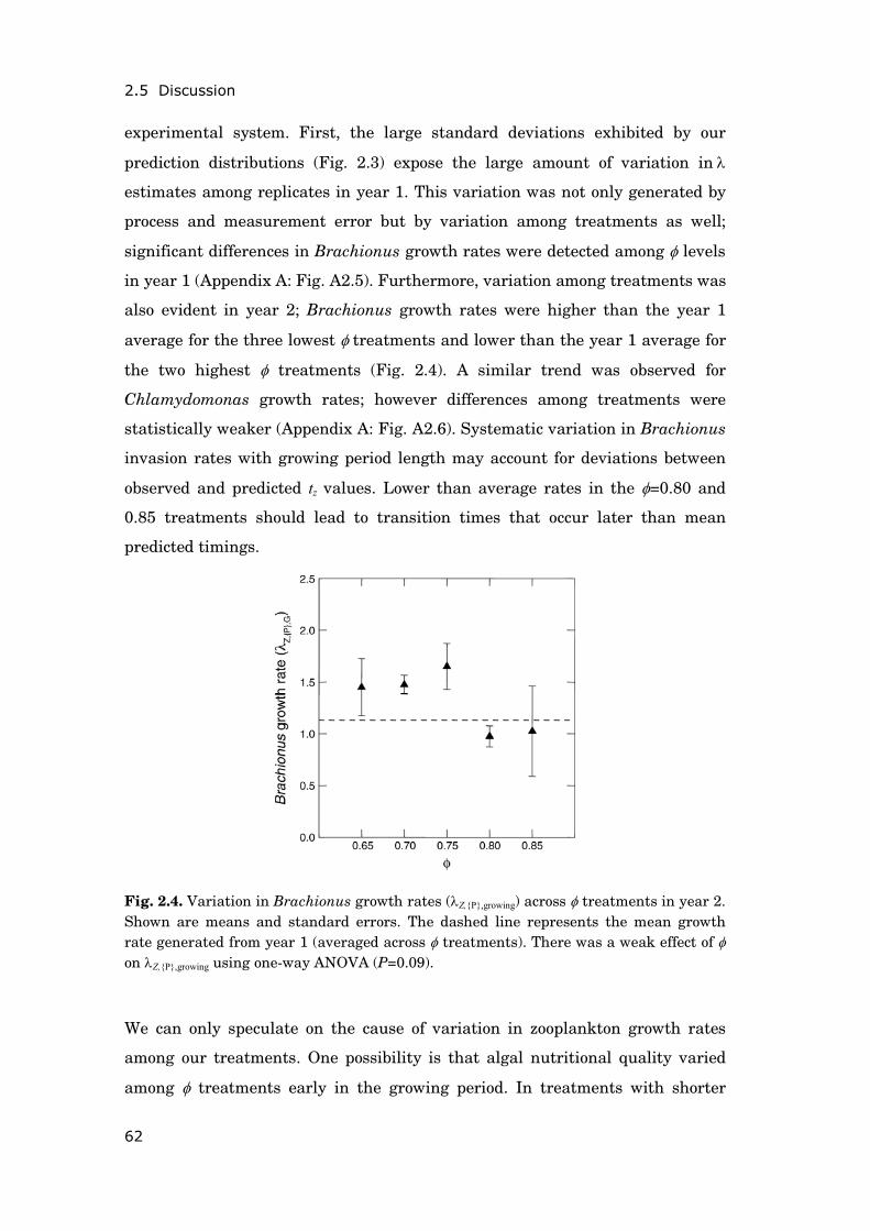
2.5 Discussion

62

experimental system. First, the large standard deviations exhibited by our

prediction distributions (Fig. 2.3) expose the large amount of variation in λ

estimates among replicates in year 1. This variation was not only generated by

process and measurement error but by variation among treatments as well;

significant differences in Brachionus growth rates were detected among φ levels

in year 1 (Appendix A: Fig. A2.5). Furthermore, variation among treatments was

also evident in year 2; Brachionus growth rates were higher than the year 1

average for the three lowest φ treatments and lower than the year 1 average for

the two highest φ treatments (Fig. 2.4). A similar trend was observed for

Chlamydomonas growth rates; however differences among treatments were

statistically weaker (Appendix A: Fig. A2.6). Systematic variation in Brachionus

invasion rates with growing period length may account for deviations between

observed and predicted tz values. Lower than average rates in the φ=0.80 and

0.85 treatments should lead to transition times that occur later than mean

predicted timings.

Fig. 2.4. Variation in Brachionus growth rates (λZ,{P},growing) across φ treatments in year 2. Shown are means and standard errors. The dashed line represents the mean growth rate generated from year 1 (averaged across φ treatments). There was a weak effect of φ on λZ,{P},growing using one-way ANOVA (P=0.09).

We can only speculate on the cause of variation in zooplankton growth rates

among our treatments. One possibility is that algal nutritional quality varied

among φ treatments early in the growing period. In treatments with shorter

Chapter 2

63

growing periods, Chlamydomonas populations started at much lower densities

at the initiation of the growing season and thus experienced exponential growth

for longer periods of time. For example, algal densities, on average, increased up

to four orders of magnitude in the φ=0.65 treatment and less than two orders of

magnitude in the φ=0.85 treatment in year 2 (Fig. 2.2). Algal populations that

experience nutrient saturated conditions and exponential growth for longer

periods of time should exhibit higher cellular nutrient content (i.e., lower

carbon:phosphorus and carbon:nitrogen content) and thus could be of greater

nutritional quality for zooplankton. Moreover, Chlamydomonas cells grown

under nutrient saturated conditions are known to be more easily digested by

zooplankton compared to nutrient-limited cells (van Donk et al. 1997), further

increasing the probability that algal populations in low φ treatments were of

better quality for Brachionus. Whether covariation between zooplankton

maximal growth rates and growing season length is a peculiarity of our model

system or a generalizable feature of natural planktonic systems is an open

question. While our highly simplified system may have amplified such effects, it

is not inconceivable that this phenomenon could occur in natural systems,

delaying expected zooplankton population peaks. If of sufficient magnitude, our

model could be easily altered to allow for changes in zooplankton growth rates

with changing φ in order to increase quantitative predictive power.

Finally, it is important to note the inherent mismatch between the time scales

employed in our model and experiment. The dominant forcing period in natural

aquatic ecosystems is one year. In contrast, the SSD approach assumes the

limit of infinite period forcing in which species dynamics approach log-linear (as

in Fig. 2.1A) and which maintains analytical tractability (Klausmeier

unpublished manuscript). Numerical results show that this approximation is

reasonable for systems forced at the annual scale (Klausmeier unpublished

manuscript). Our laboratory system was forced with an effective period of 16.5–

21.5 days; longer periods would have required larger winter dilutions, which

would have resulted in less than one rotifer per flask in our 800 mL

experimental volumes. Thus, the time scales of our mathematical and laboratory

models varied in opposite directions from the natural systems they were

intended to mimic, potentially generating discrepancies between our predictions

2.6 Conclusions

64

and empirical results. As φ decreased in our experiments, the assumptions of the

SSD model were better met, which may account for the stronger match between

observed and predicted transition times and the better fits seen in supplemental

figures A2.1 and A2.2 (Appendix A).

2.6 Conclusions

The growing reality of climate change has necessitated more in-depth

examination of the role of seasonal forcing and altered seasonality on the

structure and dynamics of natural communities (Walther et al. 2002; Parmesan

and Yohe 2003; Menzel et al. 2006; Berger et al. 2007; Cleland et al. 2007; Huber

et al. 2008). As increases in average mean temperatures may increase the

number of ice-free days temperate lakes experience, the effective length of the

growing season is also predicted to increase. How such alterations impact the

timing of spring algal blooms and zooplankton population peaks is a vital

question facing aquatic ecologists. Our model provides a simple but tractable

framework for exploring the dynamic consequences of variation in large-scale

seasonal events. We show both theoretically and empirically that the probability

of zooplankton population persistence increases with increasing growing period.

Furthermore, the timing of zooplankton and algal population blooms depends

greatly on the relative length of the growing season with the timing of

algal/zooplankton population peaks occurring progressively earlier in the year

with increasing growing period. Such advances in the seasonal timing of

plankton population peaks have been detected in many long-term data sets (e.g.,

Winder and Schindler 2004a, 2004b; Huber et al. 2008). Our model framework

could help to better understand the mechanisms underlying such phenological

changes. Given the low number of parameters required by the approach, the

successional state dynamics framework can be easily altered to address

alternative food web structures while retaining analytical tractability. Moreover,

the model’s minimal parameter requirement has the advantage of being

relatively easy to parameterize empirically and generate quantitative

predictions. Thus, compared to more complex, process-based numerical models,

the SSD framework could be a more promising approach for generating

projections of plankton phenology under future climate warming.

Chapter 2

65

2.7 Acknowledgements

Author contributions: CFS, VH and CAK wrote the paper; CFS and VH analyzed

the data ; AS, CAK, CFS and EL designed the experiment; AS and CFS

performed the experiment; CAK and EL developed the SSD model; VH wrote the

genetic algorithm. We thank D. Shumway, P. Woodruff and A. Morgan for

laboratory assistance; M. Evans, J. Mellard, and K. Yoshiyama for valuable

comments on the manuscript; and G. Fussmann and S. Ellner for helpful advice

on model fitting. This research was supported by National Science Foundation

grant DEB-0610532 and a grant from the James S. McDonnell Foundation to

CAK and EL. VH was supported by the German Research Foundation (DFG

SPP 1162) and the German Academic Exchange Service (DAAD). This is

contribution number 1495 of the Kellogg Biological Station.

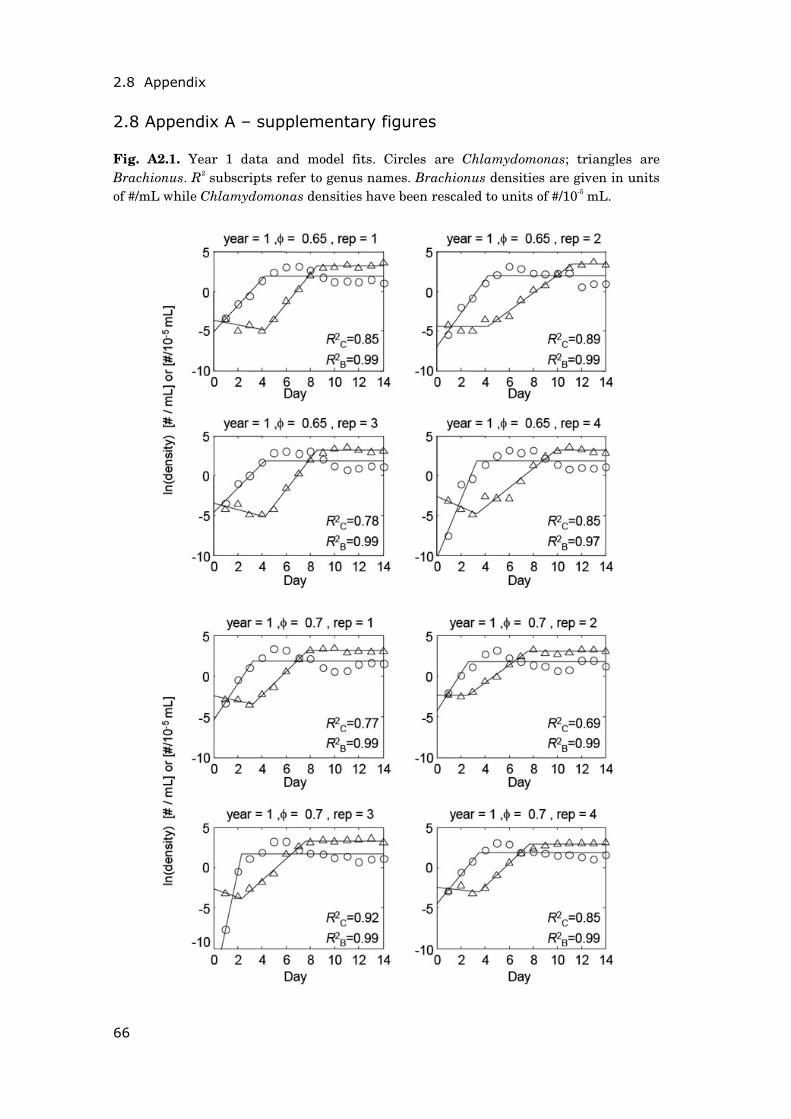
2.8 Appendix

66

2.8 Appendix A – supplementary figures

Fig. A2.1. Year 1 data and model fits. Circles are Chlamydomonas; triangles are Brachionus. R2 subscripts refer to genus names. Brachionus densities are given in units of #/mL while Chlamydomonas densities have been rescaled to units of #/10-5 mL.

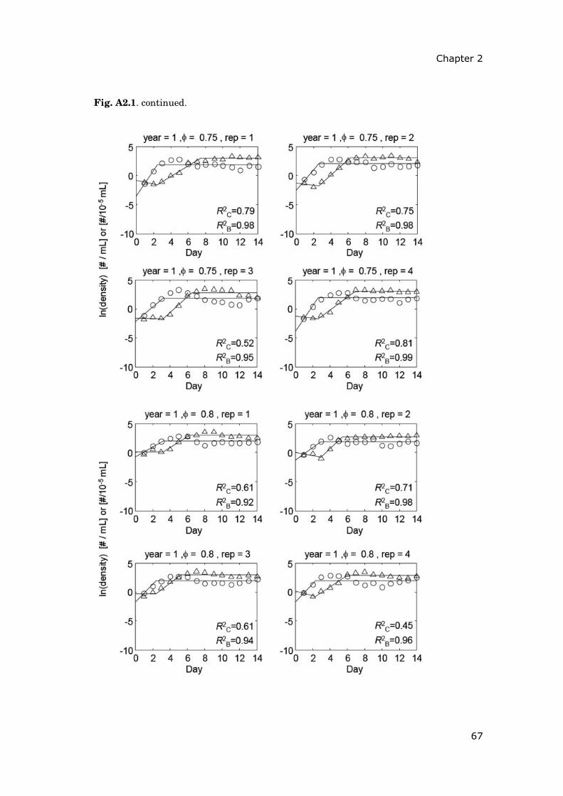
Chapter 2

67

Fig. A2.1. continued.

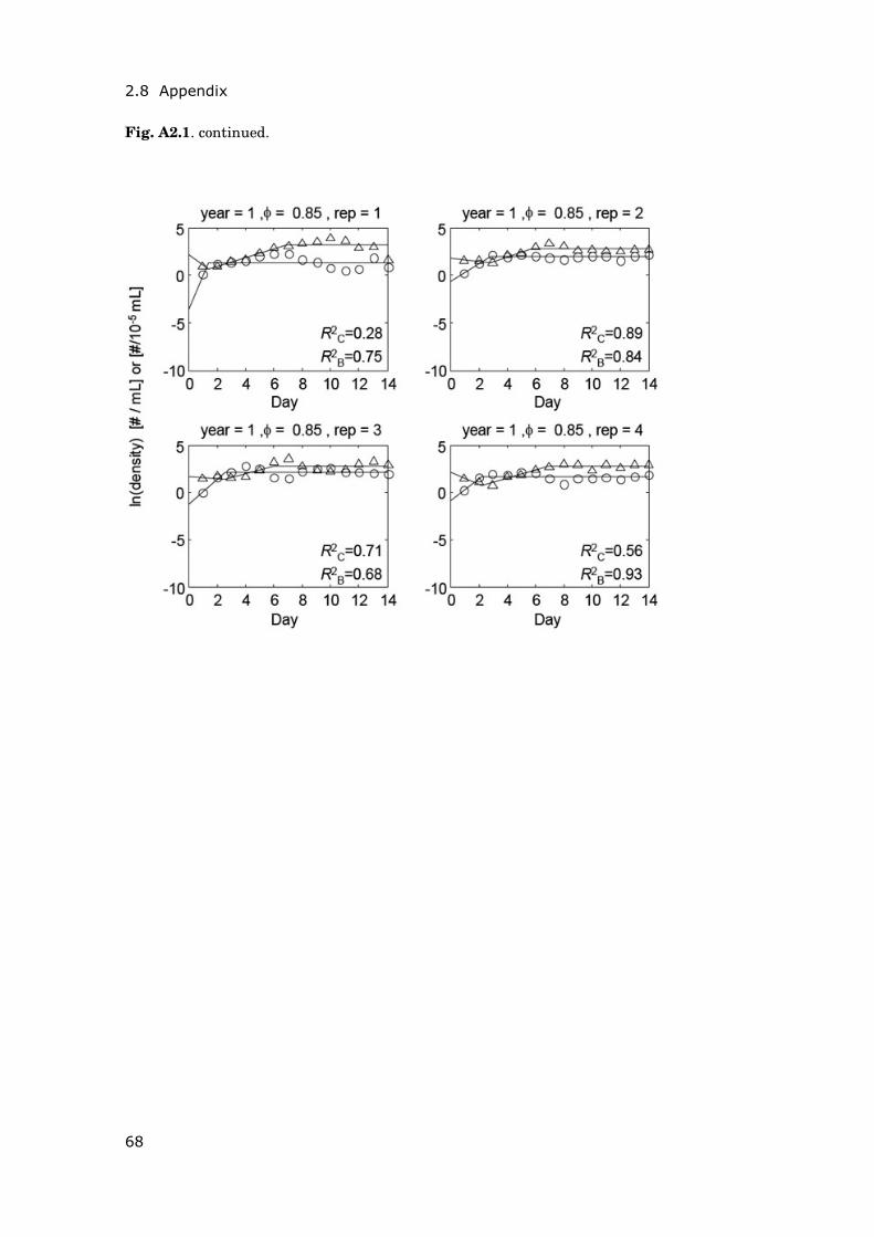
2.8 Appendix

68

Fig. A2.1. continued.

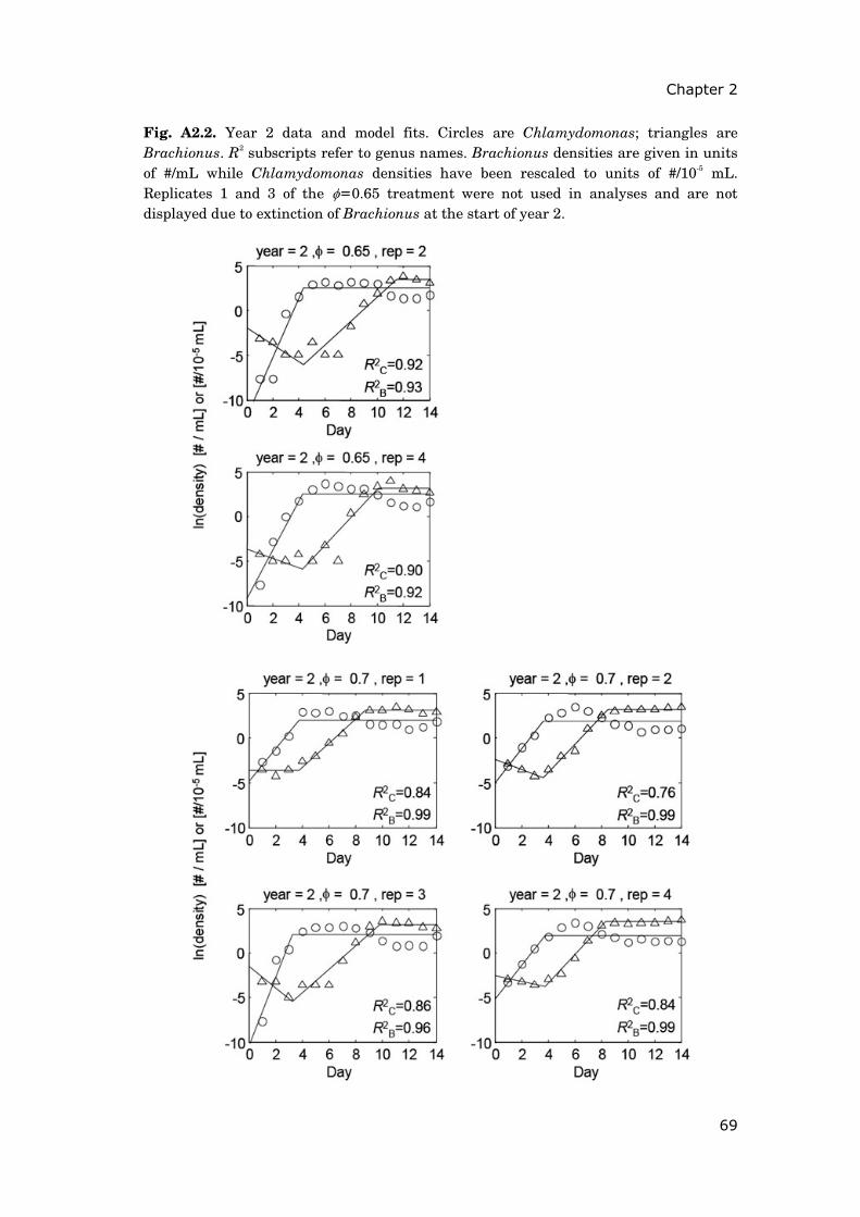
Chapter 2

69

Fig. A2.2. Year 2 data and model fits. Circles are Chlamydomonas; triangles are Brachionus. R2 subscripts refer to genus names. Brachionus densities are given in units of #/mL while Chlamydomonas densities have been rescaled to units of #/10-5 mL. Replicates 1 and 3 of the φ=0.65 treatment were not used in analyses and are not displayed due to extinction of Brachionus at the start of year 2.

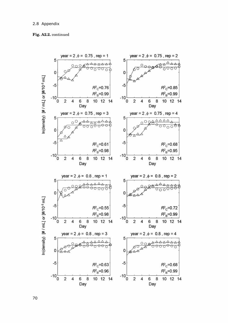
2.8 Appendix

70

Fig. A2.2. continued

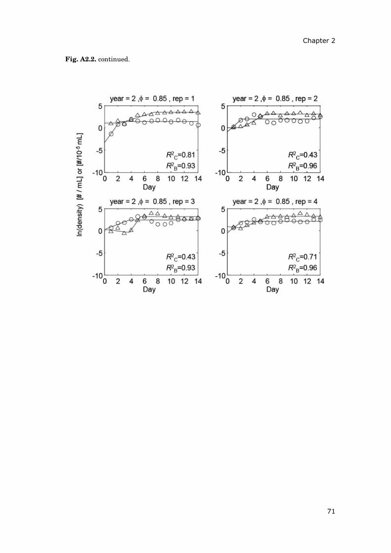
Chapter 2

71

Fig. A2.2. continued.

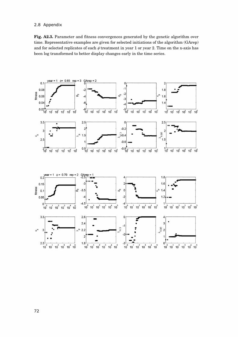
2.8 Appendix

72

Fig. A2.3. Parameter and fitness convergences generated by the genetic algorithm over time. Representative examples are given for selected initiations of the algorithm (GArep) and for selected replicates of each φ treatment in year 1 or year 2. Time on the x-axis has been log transformed to better display changes early in the time series.

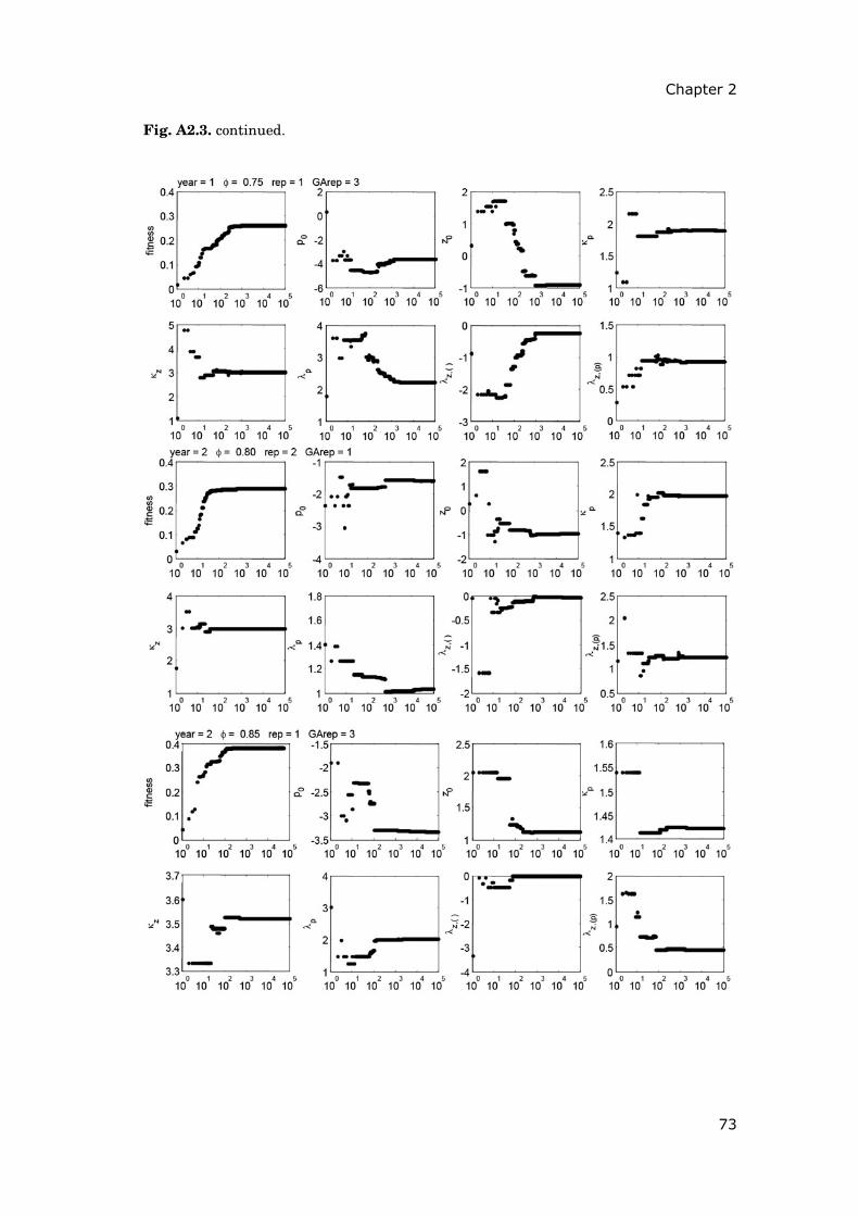
Chapter 2

73

Fig. A2.3. continued.

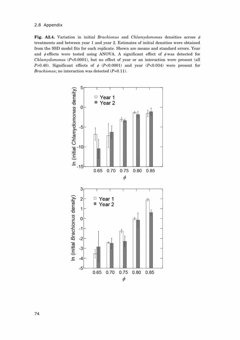
2.8 Appendix

74

Fig. A2.4. Variation in initial Brachionus and Chlamydomonas densities across φ treatments and between year 1 and year 2. Estimates of initial densities were obtained from the SSD model fits for each replicate. Shown are means and standard errors. Year and φ effects were tested using ANOVA. A significant effect of φ was detected for Chlamydomonas (P<0.0001), but no effect of year or an interaction were present (all P>0.40). Significant effects of φ (P<0.0001) and year (P<0.034) were present for Brachionus; no interaction was detected (P=0.11).

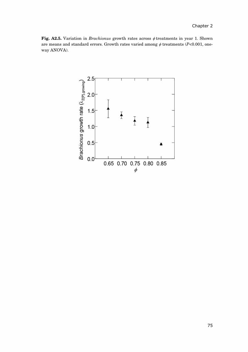
Chapter 2

75

Fig. A2.5. Variation in Brachionus growth rates across φ treatments in year 1. Shown are means and standard errors. Growth rates varied among φ treatments (P<0.001, one-way ANOVA).

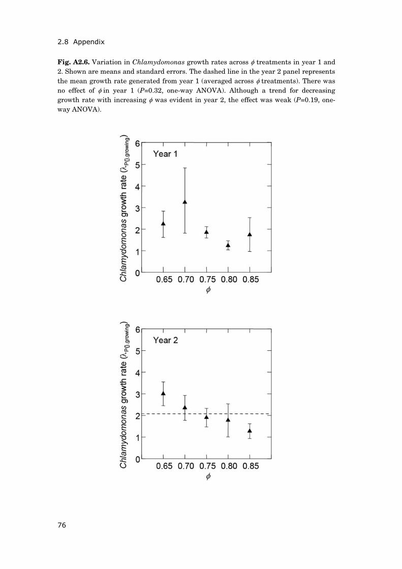
2.8 Appendix

76

Fig. A2.6. Variation in Chlamydomonas growth rates across φ treatments in year 1 and 2. Shown are means and standard errors. The dashed line in the year 2 panel represents the mean growth rate generated from year 1 (averaged across φ treatments). There was no effect of φ in year 1 (P=0.32, one-way ANOVA). Although a trend for decreasing growth rate with increasing φ was evident in year 2, the effect was weak (P=0.19, one-way ANOVA).

Chapter 2

77

2.9 Appendix B – description of the genetic algorithm

The genetic algorithm was based on a procedure used by Tietjen and Huth

(2006) and Huber et al. (2008). For a more general introduction to genetic

algorithms see Haupt and Haupt (1998). It was initialized by creating a suite of

64 parameter sets. Each set consisted of 7 parameters (the growth rates

λP,{},growing, λZ,{},growing, λZ,{P},growing, the density thresholds Kp, Kz, and the initial

densities P0, Z0). The parameters were drawn randomly from intervals defined

by visually inspecting the data. The genetic algorithm was run for each replicate

of the five period length treatments (φ = 0.65, 0.7, 0.75, 0.8 and 0.85) separately.

Once initiated, each generation of the genetic algorithm was composed of the

following steps:

a) Selection of the best parameter set: For each parameter set the

trajectories of the SSD model (Fig. 2.1A) were established by numerically

determining timing and densities at transitions tp and tz (for details see

Klausmeier unpublished manuscript). After interpolation of trajectories,

fitness F of each parameter set was evaluated by assessing the inverse of

the sum of squared differences in observed and predicted densities

( )∑ −= 2

1predictedobserved

F . Then, a total of 8 parameter sets were

selected: the two sets that produced the highest fitness and six other

parameter sets chosen randomly with a probability proportional to their

fitness.

b) Crossover: A new suite of parameter sets was constructed by recombining

all possible pairs of the selected parameter sets. The recombination

consisted of cutting the parameter string of two sets at a random position

and creating two new sets by combining the corresponding parts of the

parameter strings.

c) Mutation: After recombination, random changes were imposed on

parameters with a mutation rate of 0.1 (except for the parameter set that

had produced the best performance). The magnitude of mutation, added

to the current parameter value, was drawn from a normal distribution

N(0,σm) where σm was 1 for thresholds and initial densities and 0.5 for

growth rates. If growth rates underwent a sign change during the

2.8 Appendix

78

mutation procedure, the magnitude of mutation was alternatively drawn

from a uniform distribution between zero and the current parameter

value.

These steps were repeated for 300 000 generations. Last, the parameter set with

the highest fitness in the final selection procedure provided the default

parameter estimates. We applied several test runs of the genetic algorithm to

make sure that the chosen number of generations was sufficient for convergence.

The convergence criterion applied was that the parameter estimates for three

independent initializations of the genetic algorithm did not differ more than by

0.1 in the first decimal place. Example plots showing that parameters converged

quickly to their default values can be found in Appendix A.

Chapter 3

To bloom or not to bloom: contrasting development of cyanobacteria

during the European heat waves of 2003 and 2006 in a shallow lake

_____________________________________

In revision for Global Change Biology as Huber V., C. Wagner, D. Gerten and R. Adrian. To bloom or not to bloom: contrasting development of cyanobacteria

during the European heat waves of 2003 and 2006 in a shallow lake.

3.1 Abstract

80

3.1 Abstract

Heat wave events might give us a glance of the climate to come and therefore

allow investigating how ecosystems could evolve in the future. In nutrient-rich

freshwater systems, harmful blooms of cyanobacteria are considered to be

promoted under heat wave conditions, posing a threat to water quality. Here the

effects of the Central European summer heat waves in 2003 and 2006 on

cyanobacteria of a eutrophic, shallow lake were evaluated. While a bloom of

cyanobacteria developed in 2006 according to expectations, cyanobacteria

surprisingly remained at a record-low during the entire summer of 2003. Results

of classification tree analysis based on a long-term (1993-2007) data set of

physical, chemical and biological variables suggested that differences in air

temperature and wind speed and related differences in the timing, intensity and

duration of thermal stratification were the main reasons for the contrasting

development of cyanobacteria. In addition to seasonal patterns of heat wave

conditions, which were less favourable for blooms in 2003 than in 2006,

differences in grazer (daphnid) abundance might have also contributed to the

suppression of a cyanobacteria bloom in 2003. Our findings point to the

importance of local weather patterns and caution against conclusions on climate

change as a catalyst of cyanobacteria blooms that are drawn from single extreme

events and that consider meteorological conditions averaged over large temporal

scales only.

Chapter 3

81

3.2 Introduction

Central Europe has recently experienced several extreme heat waves, most

prominently the summer heat wave of 2003. Mean air temperature in the

summer of that year exceeded the long-term average by around 3°C over a large

area (Schär et al. 2004). Similarly, mean air temperatures in July 2006 locally

were up to 5°C higher than on average (Struzewska and Kaminski 2008).

Assessing the impacts of such extreme weather conditions on ecosystems is

important, especially because summer heat waves are expected to occur more

frequently under future climate warming (Meehl and Tebaldi 2004; Schär and

Jendritzky 2004). Aquatic ecosystems have been shown to be strongly affected

by the summer heat wave of 2003 (Jankowski et al. 2006; Daufresne et al. 2007;

Wilhelm and Adrian 2007); in particular, the occurrence of harmful

cyanobacteria blooms was promoted in some nutrient-rich water bodies (Paerl

and Huisman 2008; Jöhnk et al. 2008).

Cyanobacteria pose a threat to water quality in many aquatic ecosystems

(Huisman et al. 2005). Therefore, the factors that induce blooms of harmful

cyanobacteria have been the subject of intensive research in the past decades. It

is well established knowledge that nutrient enrichment of water bodies

(eutrophication) enhances the risk of cyanobacteria blooms (Huisman and Hulot

2005). Considering that cyanobacteria species can differ quite substantially in

functional attributes (e.g., nitrogen fixing, buoyancy), generalization of processes

promoting blooms is difficult (Hyenstrand et al. 1998; Dokulil and Teubner

2000). However, high concentrations of total phosphorus and total nitrogen

(Downing et al. 2001) and also low supply ratios of nitrogen to phosphorus

(Smith 1983) have been shown to correlate with high biomass of cyanobacteria

in many systems.

More recently, scientists have turned their attention to the question of climate

change as a potential catalyst for the extension and intensification of

cyanobacteria blooms (de Senerpont Domis et al. 2007b; Paerl and Huisman

2008). Besides possible indirect effects such as climate-induced nutrient

enrichment, cyanobacteria are thought to be directly favoured by rising water

temperatures, as their high temperature optima for growth (e.g., around 28 °C

3.3 Methods

82

for the cyanobacteria species Microcystis sp.) give them a competitive advantage

over other algae in warm water (Butterwick et al. 2005; Jöhnk et al. 2008). In

eutrophic water bodies, buoyant cyanobacteria species are also known to benefit

from intensified and prolonged thermal stratification that often co-occurs with

high water temperatures (Huisman et al. 2005). When the stability of the water

column is high, their buoyancy enables them to float to the surface and out-

compete other algae for light (Huisman et al. 2004).

Cyanobacteria blooms have been observed in the nutrient-rich shallow lake

studied here (Müggelsee) during most summers since the start of a monitoring

program in 1979. The lake, located in north-eastern Germany, was under the

influence of the European summer heat waves of 2003 and 2006. Despite

similarly favourable physical conditions (high water temperatures and relatively

strong thermal stratification) at times of anomalously hot weather

cyanobacteria bloomed strongly in the summer of 2006, but remained at a record

low during all of 2003.

Recently, Wagner and Adrian (2009) used classification tree analysis to identify

the main environmental factors that determine the contribution of

cyanobacteria to total phytoplankton biovolume in Müggelsee. They showed that

while high total phosphorus concentration was the best indicator of elevated

cyanobacteria contribution, intensified and prolonged thermal stratification also

promoted cyanobacterial dominance in this polymictic lake. Here, we used the

critical thresholds of environmental factors determined by Wagner and Adrian

(2009) to investigate the reasons for the surprisingly contrasting development of

cyanobacteria during the heat wave summers of 2003 and 2006. Classification

tree analysis was also applied to characterize meteorological conditions that

favour thermal stratification in the lake.

3.3 Methods

Study sites and data basis—Müggelsee (52°26’ N, 13°39’ E) is a polymictic,

shallow lake (mean depth 4.9 m, maximum depth 7.9 m) with a surface area of

7.3 km2. An ongoing sampling program has collected data on plankton, physical

and chemical variables, with biweekly sampling in winter and weekly sampling

Chapter 3

83

in summer, beginning in 1979 (Driescher et al. 1993). Since the start of this

sampling program the lake has experienced an increase in water temperature

(around 0.5 °C per decade in summer) and quasi-simultaneously a decrease in

nutrient loading (Köhler et al. 2005; Huber et al. 2008). To restrict confounding

effects of a change in trophic state (Köhler et al. 2005) and also due to missing

data for total nitrogen prior to 1993, analyses were restricted to 1993-2007, the

eutrophic phase of the lake. Intermittent thermal stratification during summer

is common in this shallow lake (exposed to prevailing south-westerly winds),

with consequent effects on water temperature, oxygen, internal nutrient load,

and phytoplankton development (Wilhelm and Adrian 2008).

Weekly profile measurements (0-5 m depth at 0.5 m intervals) of water

temperature (°C) were used to calculate the Schmidt stability index (g cm cm-2)

according to Soranno (1997), which assesses the intensity of thermal

stratification of the water column:

zAzsASz

sssi Δ−−= ∑

=

−max

0

10 *)*)(( ρρ (1)

where A0 the surface area of the lake, As lake area at depth s; ps density

calculated from water temperature at depth s, ρ* mean density; z* depth where

mean density occurs, zmax maximum depth, and Δz depth interval of 1 m.

We considered the lake to be thermally stratified when the difference in water

temperature between the surface and at 5 m depth was > 1°C (Wilhelm and

Adrian 2008; Wagner and Adrian 2009). High frequency data (available from an

automatic measurement station on the lake since 2003) revealed that the weekly

data of water temperature used here is a good indicator of the timing and

duration of thermal stratification events that last longer than 1 week (Wagner

and Adrian 2009). Only one of six thermal stratification events > 1 week

observed between 2003 and 2006 was misclassified in duration (Wagner and

Adrian 2009). All nutrient concentrations (total nitrogen (TN, mg L-1), total

phosphorus (TP, μg L-1), and soluble reactive phosphorus (SRP, μg L-1)) and

plankton abundance used in this study (see below) were determined from

volumetrically weighted mixed samples in the absence of thermal stratification,

while only the upper 3.5 m of the water column, corresponding to the average

3.3 Methods

84

epilimnetic depth, were taken into account when the lake was stratified

(Wilhelm and Adrian 2008).

Algal biovolumes (mm3 L-1) were determined using standard limnological

techniques, based on microscope counts and individually measured cell volumes

(Driescher et al. 1993). However, data on individual cell and filament volumes

(μm3 ind-1) were not accessible prior to 1999. Data resolved to phytoplankton

species level was summed to yield time-series of total phytoplankton,

cyanobacteria, cryptophytes, and the cyanobacteria genus Anabaena, which was

dominant during the summer of 2006. Since individual body size of zooplankton

was not directly measured we used the available abundance data (ind. L-1) to

construct time-series of the main zooplankton groups, daphnids and cyclopoid

copepods. Given that grazing pressure on phytoplankton is closely linked to

zooplankton body size (Sterner 1989; Adrian and Frost 1992) we cannot exclude

that the lack of individual body-size measurements introduced a certain bias.

However, daphnid and cyclopoid copepod species composition was similar in the

heat wave summers of 2003 and 2006 (dominating species were Daphnia

cucullata, and Mesocyclops sp. and Thermocyclops sp., respectively, in both

years). This similarity made us confident that differences in abundance also

translated into differences in grazing pressure, at least in these two years.

Mean weekly measurements of meteorological variables were provided by the

nearby weather station Schöneiche (~ 4 km to the northeast of Müggelsee) for

1993-2006. In addition to Müggelsee, data of mean cyanobacteria biovolume

during the summers of 2003 and 2006 in eight other mesotrophic to

hypertrophic lakes of north-eastern Germany was available from the German

national lake phytoplankton data base compiled by Mischke (2008; LAWA-

project O9.08; unpublished data). Summer was defined as the period from June

to August.

Classification tree analysis—Classification tree analysis is a nonparametric,

recursive data-mining technique that produces a collection of rules, involving

thresholds of key predictor variables, to best explain variability in a categorical

response variable (for further details see Wagner and Adrian 2009; Breiman et

al. 1993). When applying this method to cyanobacteria data, Wagner and Adrian

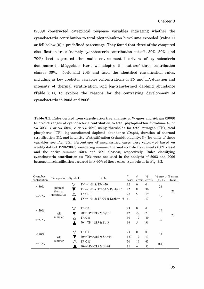
Chapter 3

85

(2009) constructed categorical response variables indicating whether the

cyanobacteria contribution to total phytoplankton biovolume exceeded (value 1)

or fell below (0) a predefined percentage. They found that three of the computed

classification trees (namely cyanobacteria contribution cut-offs 30%, 50%, and

70%) best separated the main environmental drivers of cyanobacteria

dominance in Müggelsee. Here, we adopted the authors’ three contribution

classes 30%, 50%, and 70% and used the identified classification rules,

including as key predictor variables concentrations of TN and TP, duration and

intensity of thermal stratification, and log-transformed daphnid abundance

(Table 3.1), to explore the reasons for the contrasting development of

cyanobacteria in 2003 and 2006.

Table 3.1. Rules derived from classification tree analysis of Wagner and Adrian (2009) to predict ranges of cyanobacteria contribution to total phytoplankton biovolume (< or >= 30%, < or >= 50%, < or >= 70%) using thresholds for total nitrogen (TN), total phosphorus (TP), log-transformed daphnid abundance (Daph), duration of thermal stratification (Sd), and intensity of stratification (Schmidt stability, Si) (for units of these variables see Fig. 3.2). Percentages of misclassified cases were calculated based on weekly data of 1993-2007, considering summer thermal stratification events (30% class) and the entire summer (50% and 70% classes), respectively. Rules classifying cyanobacteria contribution >= 70% were not used in the analysis of 2003 and 2006 because misclassification occurred in > 60% of these cases. Symbols as in Fig. 3.3.

Cyanobact. contribution Time period Symbol Rule #

cases # errors

% errors

% errors (< / >)

% errorstotal

TN<=1.01 & TP<=70 12 0 0 < 30%

TN<=1.01 & TP>70 & Daph>1.6 22 8 36 24

TN>1.01 27 5 19 >=30%

Summer thermal

stratification TN<=1.01 & TP>70 & Daph<=1.6 6 1 17

18 21

TP<70 23 0 0

< 50% 70<=TP<=215 & Sd<=3 127 29 23

19

TP>215 30 12 40 >=50%

All summer

70<=TP<=215 & Sd>3 16 5 31 37

23

TP<70 23 0 0

< 70% 70<=TP<=215 & Si<=44 127 17 13

11

TP>215 30 19 63 >=70%

All summer

70<=TP<=215 & Si>44 11 6 55 (61)

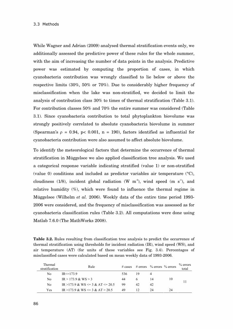
3.3 Methods

86

While Wagner and Adrian (2009) analysed thermal stratification events only, we

additionally assessed the predictive power of these rules for the whole summer,

with the aim of increasing the number of data points in the analysis. Predictive

power was estimated by computing the proportion of cases, in which

cyanobacteria contribution was wrongly classified to lie below or above the

respective limits (30%, 50% or 70%). Due to considerably higher frequency of

misclassification when the lake was non-stratified, we decided to limit the

analysis of contribution class 30% to times of thermal stratification (Table 3.1).

For contribution classes 50% and 70% the entire summer was considered (Table

3.1). Since cyanobacteria contribution to total phytoplankton biovolume was

strongly positively correlated to absolute cyanobacteria biovolume in summer

(Spearman’s ρ = 0.94, p< 0.001, n = 190), factors identified as influential for

cyanobacteria contribution were also assumed to affect absolute biovolume.

To identify the meteorological factors that determine the occurrence of thermal

stratification in Müggelsee we also applied classification tree analysis. We used

a categorical response variable indicating stratified (value 1) or non-stratified

(value 0) conditions and included as predictor variables air temperature (°C),

cloudiness (1/8), incident global radiation (W m-2), wind speed (m s-1), and

relative humidity (%), which were found to influence the thermal regime in

Müggelsee (Wilhelm et al. 2006). Weekly data of the entire time period 1993-

2006 were considered, and the frequency of misclassification was assessed as for

cyanobacteria classification rules (Table 3.2). All computations were done using

Matlab 7.6.0 (The MathWorks 2008).

Table 3.2. Rules resulting from classification tree analysis to predict the occurrence of thermal stratification using thresholds for incident radiation (IR), wind speed (WS), and air temperature (AT) (for units of these variables see Fig. 3.4). Percentages of misclassified cases were calculated based on mean weekly data of 1993-2006.

Thermal stratification Rule # cases # errors % errors % errors % errors

total No IR<=173.9 536 19 4 No IR > 173.9 & WS > 3 44 6 14 No IR >173.9 & WS <= 3 & AT <= 20.5 99 42 42

10

Yes IR >173.9 & WS <= 3 & AT > 20.5 49 12 24 24

11

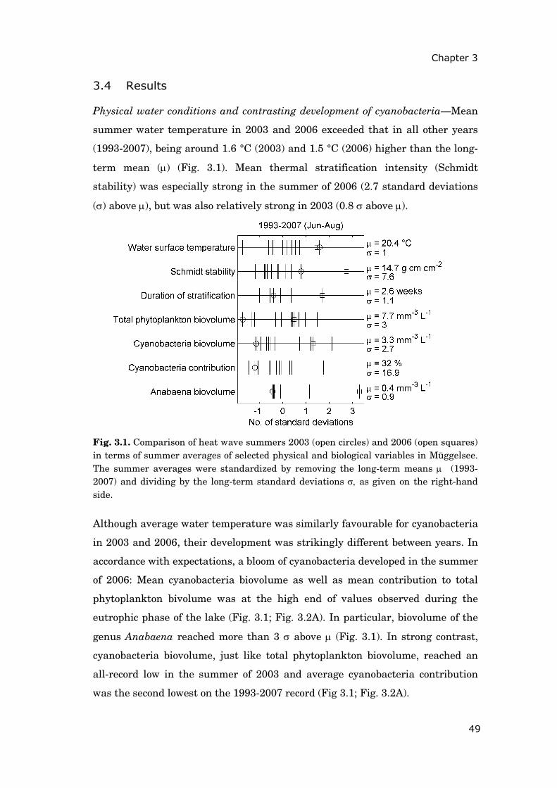
Chapter 3

49

3.4 Results

Physical water conditions and contrasting development of cyanobacteria—Mean

summer water temperature in 2003 and 2006 exceeded that in all other years

(1993-2007), being around 1.6 °C (2003) and 1.5 °C (2006) higher than the long-

term mean (μ) (Fig. 3.1). Mean thermal stratification intensity (Schmidt

stability) was especially strong in the summer of 2006 (2.7 standard deviations

(σ) above μ), but was also relatively strong in 2003 (0.8 σ above μ).

Fig. 3.1. Comparison of heat wave summers 2003 (open circles) and 2006 (open squares) in terms of summer averages of selected physical and biological variables in Müggelsee. The summer averages were standardized by removing the long-term means μ (1993-2007) and dividing by the long-term standard deviations σ, as given on the right-hand side.

Although average water temperature was similarly favourable for cyanobacteria

in 2003 and 2006, their development was strikingly different between years. In

accordance with expectations, a bloom of cyanobacteria developed in the summer

of 2006: Mean cyanobacteria biovolume as well as mean contribution to total

phytoplankton bivolume was at the high end of values observed during the

eutrophic phase of the lake (Fig. 3.1; Fig. 3.2A). In particular, biovolume of the

genus Anabaena reached more than 3 σ above μ (Fig. 3.1). In strong contrast,

cyanobacteria biovolume, just like total phytoplankton biovolume, reached an

all-record low in the summer of 2003 and average cyanobacteria contribution

was the second lowest on the 1993-2007 record (Fig 3.1; Fig. 3.2A).

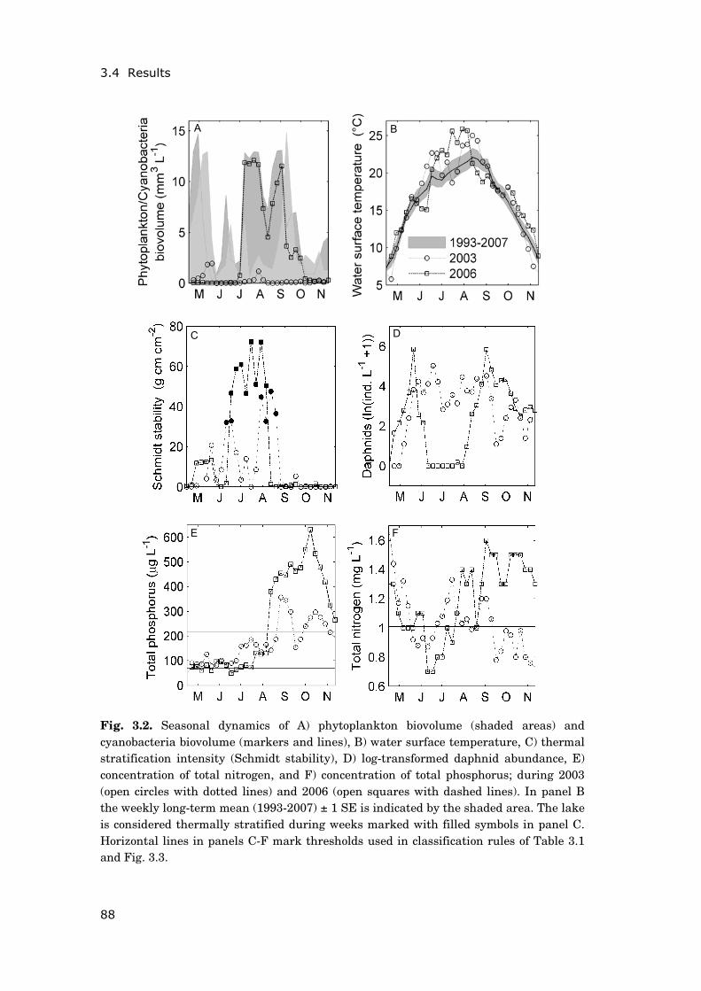
3.4 Results

88

Fig. 3.2. Seasonal dynamics of A) phytoplankton biovolume (shaded areas) and cyanobacteria biovolume (markers and lines), B) water surface temperature, C) thermal stratification intensity (Schmidt stability), D) log-transformed daphnid abundance, E) concentration of total nitrogen, and F) concentration of total phosphorus; during 2003 (open circles with dotted lines) and 2006 (open squares with dashed lines). In panel B the weekly long-term mean (1993-2007) ± 1 SE is indicated by the shaded area. The lake is considered thermally stratified during weeks marked with filled symbols in panel C. Horizontal lines in panels C-F mark thresholds used in classification rules of Table 3.1 and Fig. 3.3.

A B

C D

E F

Chapter 3

89

Seasonal patterns of water temperature and thermal stratification—As a first

step to better understand the striking contrast in cyanobacteria development,

we considered the seasonal patterns of water temperature and thermal

stratification. While the water temperature was continuously above the long-

term average from mid-June to mid-August in 2006, two separated periods of

relatively warm water were observed in June and August of 2003 (Fig. 3.2B).

The mixing regime of the lake followed the same pattern: an 8-week period of

continuous thermal stratification in 2006, and by contrast two shorter

stratification periods (of 2 and 4 weeks) in 2003 (Fig. 3.2C). Due to the

intermittent mixing event in July of 2003 the mean duration of stratification

was around average in this summer, despite a relatively strong intensity of

stratification (Fig. 3.1). As follows, we investigated whether this mixing event

was a sufficient explanation for the surprisingly low biovolume of cyanobacteria

in 2003 or whether other environmental factors were also influential.

Rule-based predictions of cyanobacteria contribution to total phytoplankton

biovolume—Mean frequencies of misclassification of cyanobacteria contribution

to total phytoplankton biovolume (calculated based on 1993-2007) were ~21%,

~23% and ~11% for contribution classes 30%, 50%, and 70%, respectively (Table

3.1). These values gave us confidence that the selected classification rules

derived from Wagner and Adrian (2009) provide insight into the environmental

factors that caused the outstanding difference in cyanobacteria development in

2003 and 2006.

Classification rules suggested that for much of the summer 2003 the insufficient

duration of thermal stratification (<= 3 weeks) was the determinant factor that

kept cyanobacteria contribution below 50% (Fig. 3.3C). Except for one week in

early July, observed cyanobacteria contribution indeed remained below 50%

during this time. The duration of stratification reached the critical threshold of 4

weeks, allowing for cyanobacteria dominance according to the classification

rules, only once in August 2003. By contrast, in 2006 missing or insufficiently

long stratification (<= 3 weeks) was predicted to prevent the dominance of

cyanobacteria early in the summer only (Fig. 3.3D). During all of July 2006,

3.4 Results

90

cyanobacteria contribution was correctly classified to lie above 50% due to an

extended period of stratification (> 3 weeks).

Comparing 2003 and 2006 in terms of intensity of thermal stratification gave a

similar picture: while insufficiently strong stratification (Schmidt stability <= 44

g cm cm-2) prevented a pronounced dominance (>= 70%) of cyanobacteria once in

early summer of 2006 only, the intensity of stratification fell below the critical

threshold several times during the summer of 2003 (Fig. 3.2C; Fig. 3.3E,F). In

all of these cases, predictions well matched observations. Thus, it appears from

this analysis that differences in thermal stratification pattern were indeed at

least one of the reasons why cyanobacteria contribution to total phytoplankton

biovolume stayed low in 2003 while it reached high values in 2006.

After the breakdown of thermal stratification in August of both years (Fig.

3.2C), high TP concentrations (> 215 μg L-1; Fig. 3.2E) apparently favoured

cyanobacteria dominance. However, while in 2006 cyanobacteria contribution

exceeded 50% during much of this period (Fig. 3.3D), it stayed extremely low in

2003 despite high TP concentrations (Fig. 3.3C). Very unfavourable TP

concentrations, below the lower critical threshold (< 70 μg L-1), occurred in early

summer of 2006 (Fig. 3.2E; Fig. 3.3B,D,F), but were never prevailing in 2003.

During the two weeks that preceded that breakdown of thermal stratification in

August 2003 (Fig. 3.2C) cyanobacteria contribution was predicted to lie below

30% because concentrations of TN and log-transformed daphnid abundance had

crossed their critical thresholds (<= 1.1 mg L-1 and >1.6 ind. L-1, respectively)

(Fig. 3.2D,F and Fig. 3.3A). In contrast, cyanobacteria contribution was

classified to be above 30% for six of the eight weeks of stratification in 2006, due

to low daphnid abundance (<=1.6 ind. L-1) and high TN concentrations (> 1.1 mg

L-1) (Fig. 3.3B). In accordance with these predictions, cyanobacteria contribution

was observed below and above 30%, respectively (Fig. 3.3A,B).

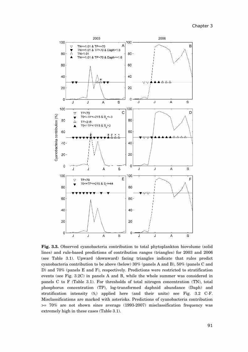
Chapter 3

91

Fig. 3.3. Observed cyanobacteria contribution to total phytoplankton biovolume (solid lines) and rule-based predictions of contribution ranges (triangles) for 2003 and 2006 (see Table 3.1). Upward (downward) facing triangles indicate that rules predict cyanobacteria contribution to be above (below) 30% (panels A and B), 50% (panels C and D) and 70% (panels E and F), respectively. Predictions were restricted to stratification events (see Fig. 3.2C) in panels A and B, while the whole summer was considered in panels C to F (Table 3.1). For thresholds of total nitrogen concentration (TN), total phosphorus concentration (TP), log-transformed daphnid abundance (Daph) and stratification intensity (Si) applied here (and their units) see Fig. 3.2 C-F. Misclassifications are marked with asterisks. Predictions of cyanobacteria contribution >= 70% are not shown since average (1993-2007) misclassification frequency was extremely high in these cases (Table 3.1).

2003 2006

A B

C D

E F

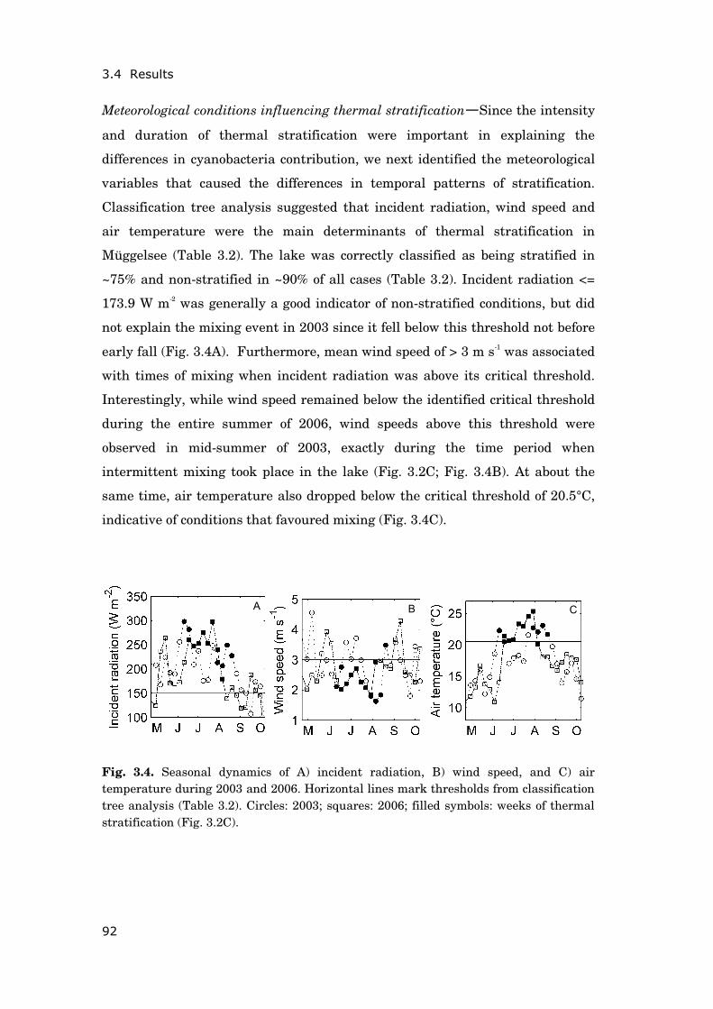
3.4 Results

92

Meteorological conditions influencing thermal stratification—Since the intensity

and duration of thermal stratification were important in explaining the

differences in cyanobacteria contribution, we next identified the meteorological

variables that caused the differences in temporal patterns of stratification.

Classification tree analysis suggested that incident radiation, wind speed and

air temperature were the main determinants of thermal stratification in

Müggelsee (Table 3.2). The lake was correctly classified as being stratified in

~75% and non-stratified in ~90% of all cases (Table 3.2). Incident radiation <=

173.9 W m-2 was generally a good indicator of non-stratified conditions, but did

not explain the mixing event in 2003 since it fell below this threshold not before

early fall (Fig. 3.4A). Furthermore, mean wind speed of > 3 m s-1 was associated

with times of mixing when incident radiation was above its critical threshold.

Interestingly, while wind speed remained below the identified critical threshold

during the entire summer of 2006, wind speeds above this threshold were

observed in mid-summer of 2003, exactly during the time period when

intermittent mixing took place in the lake (Fig. 3.2C; Fig. 3.4B). At about the

same time, air temperature also dropped below the critical threshold of 20.5°C,

indicative of conditions that favoured mixing (Fig. 3.4C).

Fig. 3.4. Seasonal dynamics of A) incident radiation, B) wind speed, and C) air temperature during 2003 and 2006. Horizontal lines mark thresholds from classification tree analysis (Table 3.2). Circles: 2003; squares: 2006; filled symbols: weeks of thermal stratification (Fig. 3.2C).

A B C

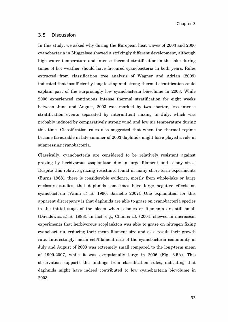
Chapter 3

93

3.5 Discussion

In this study, we asked why during the European heat waves of 2003 and 2006

cyanobacteria in Müggelsee showed a strikingly different development, although

high water temperature and intense thermal stratification in the lake during

times of hot weather should have favoured cyanobacteria in both years. Rules

extracted from classification tree analysis of Wagner and Adrian (2009)

indicated that insufficiently long-lasting and strong thermal stratification could

explain part of the surprisingly low cyanobacteria biovolume in 2003. While

2006 experienced continuous intense thermal stratification for eight weeks

between June and August, 2003 was marked by two shorter, less intense

stratification events separated by intermittent mixing in July, which was

probably induced by comparatively strong wind and low air temperature during

this time. Classification rules also suggested that when the thermal regime

became favourable in late summer of 2003 daphnids might have played a role in

suppressing cyanobacteria.

Classically, cyanobacteria are considered to be relatively resistant against

grazing by herbivorous zooplankton due to large filament and colony sizes.

Despite this relative grazing resistance found in many short-term experiments

(Burns 1968), there is considerable evidence, mostly from whole-lake or large

enclosure studies, that daphnids sometimes have large negative effects on

cyanobacteria (Vanni et al. 1990; Sarnelle 2007). One explanation for this

apparent discrepancy is that daphnids are able to graze on cyanobacteria species

in the initial stage of the bloom when colonies or filaments are still small

(Davidowicz et al. 1988). In fact, e.g., Chan et al. (2004) showed in microcosm

experiments that herbivorous zooplankton was able to graze on nitrogen fixing

cyanobacteria, reducing their mean filament size and as a result their growth

rate. Interestingly, mean cell/filament size of the cyanobacteria community in

July and August of 2003 was extremely small compared to the long-term mean

of 1999-2007, while it was exceptionally large in 2006 (Fig. 3.5A). This

observation supports the findings from classification rules, indicating that

daphnids might have indeed contributed to low cyanobacteria biovolume in

2003.

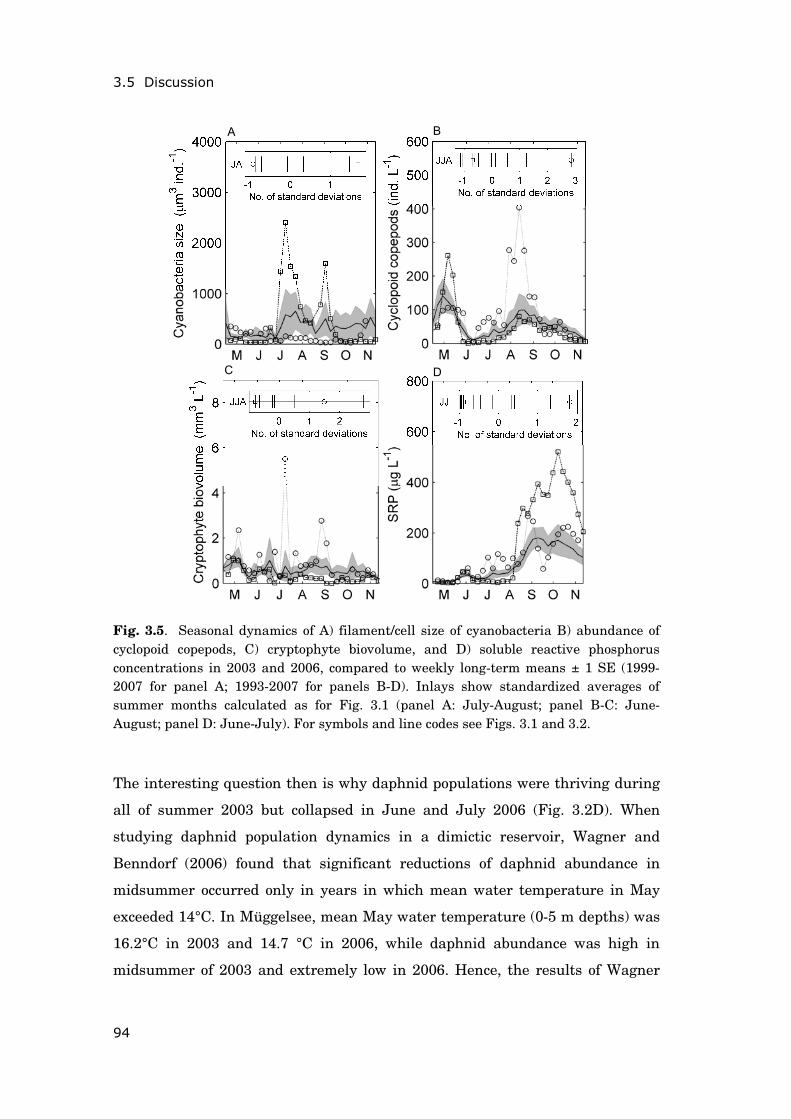
3.5 Discussion

94

Fig. 3.5. Seasonal dynamics of A) filament/cell size of cyanobacteria B) abundance of cyclopoid copepods, C) cryptophyte biovolume, and D) soluble reactive phosphorus concentrations in 2003 and 2006, compared to weekly long-term means ± 1 SE (1999-2007 for panel A; 1993-2007 for panels B-D). Inlays show standardized averages of summer months calculated as for Fig. 3.1 (panel A: July-August; panel B-C: June-August; panel D: June-July). For symbols and line codes see Figs. 3.1 and 3.2.

The interesting question then is why daphnid populations were thriving during

all of summer 2003 but collapsed in June and July 2006 (Fig. 3.2D). When

studying daphnid population dynamics in a dimictic reservoir, Wagner and

Benndorf (2006) found that significant reductions of daphnid abundance in

midsummer occurred only in years in which mean water temperature in May

exceeded 14°C. In Müggelsee, mean May water temperature (0-5 m depths) was

16.2°C in 2003 and 14.7 °C in 2006, while daphnid abundance was high in

midsummer of 2003 and extremely low in 2006. Hence, the results of Wagner

A B

C D

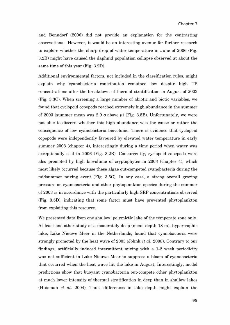
Chapter 3

95

and Benndorf (2006) did not provide an explanation for the contrasting

observations. However, it would be an interesting avenue for further research

to explore whether the sharp drop of water temperature in June of 2006 (Fig.

3.2B) might have caused the daphnid population collapse observed at about the

same time of this year (Fig. 3.2D).

Additional environmental factors, not included in the classification rules, might

explain why cyanobacteria contribution remained low despite high TP

concentrations after the breakdown of thermal stratification in August of 2003

(Fig. 3.3C). When screening a large number of abiotic and biotic variables, we

found that cyclopoid copepods reached extremely high abundance in the summer

of 2003 (summer mean was 2.9 σ above μ) (Fig. 3.5B). Unfortunately, we were

not able to discern whether this high abundance was the cause or rather the

consequence of low cyanobacteria biovolume. There is evidence that cyclopoid

copepods were independently favoured by elevated water temperature in early

summer 2003 (chapter 4), interestingly during a time period when water was

exceptionally cool in 2006 (Fig. 3.2B). Concurrently, cyclopoid copepods were

also promoted by high biovolume of cryptophytes in 2003 (chapter 4), which

most likely occurred because these algae out-competed cyanobacteria during the

midsummer mixing event (Fig. 3.5C). In any case, a strong overall grazing

pressure on cyanobacteria and other phytoplankton species during the summer

of 2003 is in accordance with the particularly high SRP concentrations observed

(Fig. 3.5D), indicating that some factor must have prevented phytoplankton

from exploiting this resource.

We presented data from one shallow, polymictic lake of the temperate zone only.

At least one other study of a moderately deep (mean depth 18 m), hypertrophic

lake, Lake Nieuwe Meer in the Netherlands, found that cyanobacteria were

strongly promoted by the heat wave of 2003 (Jöhnk et al. 2008). Contrary to our

findings, artificially induced intermittent mixing with a 1-2 week periodicity

was not sufficient in Lake Nieuwe Meer to suppress a bloom of cyanobacteria

that occurred when the heat wave hit the lake in August. Interestingly, model

predictions show that buoyant cyanobacteria out-compete other phytoplankton

at much lower intensity of thermal stratification in deep than in shallow lakes

(Huisman et al. 2004). Thus, differences in lake depth might explain the

3.5 Discussion

96

contrasting observations. In addition, the different trophic states of the two

lakes might play a role. Jöhnk et al. (2008) report extremely high mean summer

concentrations of TP and TN in Lake Nieuwe Meer in the range of ~400 μgL-1

and ~3.6 mg L-1, respectively. These concentrations largely exceed the thresholds

of 215 μgL-1 TP and ~1 mg L-1 TN found by Wagner and Adrian (2009), above

which cyanobacteria contribution to total phytoplankton biovolume tend to be

high in Müggelsee, independent of the thermal regime and daphnid abundance

(Table 3.1).

Fig. 3.6. Comparison of cyanobacteria summer biovolume in 2003 and 2006 in Müggelsee and eight geographically relatively close mesotrophic to hypertrophic lakes in north-eastern Germany. Asterisks mark data from polymictic lakes. Note different scales on y-axes. Map source: Google Earth 2009.

A survey of eight lakes of different depths and trophic states, which are

relatively close to our lake, revealed that the observation of low cyanobacteria

biovolume in 2003 and high biovolume in 2006 could neither be generalized to

geographically more neighbouring lakes (Fig. 3.6). In six of the nine lakes,

summer biovolume of cyanobacteria in 2003 exceeded the 2006 magnitude, in

contrast to the observation in Müggelsee. As for Lake Nieuwe Meer, differences

in lake depth and trophic state might be decisive, but differences in local

100 km

*

*

*

*

*

*

Chapter 3

97

weather patterns could have also been influential. Presumably, the thermal

stratification regime remained more favourable for cyanobacteria in some of

these lakes throughout the summer of 2003, because the meteorological

conditions that induced intermittent mixing in mid-summer 2003 in Müggelsee

(Fig. 3.4) did not extend to the entire region or did not impact the thermal

regimes of these lakes similarly, e.g., due to less wind-exposed sites or more

stable thermal regimes (the latter especially applicable to dimictic Arendsee,

Carwitzer See and Plöner See; Fig. 3.6). Overall, the comparisons with other

lakes re-emphasize the complexity of processes involved in the formation of

cyanobacteria blooms, making it a challenging task to project their evolution

under future climate warming.

3.6 Conclusions

Many studies have pointed to the increasing risk of cyanobacterial blooms with

climate warming. There are a number of studies indicating that many of the

lake features that are thought to change in the future, indeed, favour

cyanobacteria (Paerl and Huisman 2008). However, here we show that heat

waves do not necessarily promote cyanobacteria blooms, even not in the same

lake and when similarly high water temperatures occur. Our findings point to

the importance of seasonal weather patterns that critically determine the

thermal regime of shallow, polymictic lakes and thereby the occurrence of

cyanobacteria blooms. Albeit of secondary importance, our study also suggests

that zooplankton, which is known to be strongly sensitive to temperature and

therefore likely to be affected by heat wave events (Blenckner et al. 2007), can at

least contribute to the suppression of cyanobacteria blooms. Our results caution

against conclusions on climate change as a catalyst of cyanobacteria blooms that

are drawn from single extreme events and that consider summer averages of

meteorological conditions only. Anticipating the effects of climate change on

cyanobacteria requires a still better understanding of the complexity underlying

cyanobacteria bloom formation in lakes of different depth and trophic state.

3.7 Acknowledgements

98

3.7 Acknowledgements

We thank all scientists and technicians who have been involved in the collection

and compilation of the long-term data set of Müggelsee. We are especially

grateful to Thomas Hintze and Helgard Täuscher who helped during the

preparation of the raw data. We also acknowledge Ute Mischke who provided

data on cyanobacteria in neighbouring lakes. Katrin Tirok and three anonymous

reviewers gave extremely useful advice on earlier versions of the manuscript.

The German Research Foundation (DFG) supported Veronika Huber within the

priority program AQUASHIFT (SPP 1162).

Chapter 4

A matter of timing: heat wave impact on crustacean zooplankton

In revision for Freshwater Biology as Huber V., D. Gerten and R. Adrian. A

matter of timing: heat wave impact on crustacean zooplankton.

4.1 Abstract

100

4.1 Abstract

1. Climate change has affected zooplankton phenology and abundance in

many freshwater ecosystems. The strong temperature anomalies that

characterize summer heat waves make these events particularly suitable

to study the effects of different seasonal warming patterns on

zooplankton. Since heat waves are expected to occur more frequently

under further ongoing climate change they also allow us to investigate

how freshwater systems may be affected in the future.

2. Using a long-term data set (1991-2007) from a shallow, eutrophic lake in

Germany, we identify time periods in spring and summer during which

cyclopoid copepods and bosminids are particularly sensitive to changes in

water temperature. Based on this knowledge, we consider why summer

populations responded differently to recent heat wave events that

occurred at different times in the season.

3. Linear regressions of moving averages suggested that water

temperatures shortly before and shortly after the clear-water phase were

crucial for summer development of bosminids and cyclopoid copepods,

respectively. Algal food availability (diatoms and cryptophytes) in the

first weeks after the clear-water phase also strongly influenced the

summer populations of the two zooplankton groups.

4. Inter-annual differences in water temperature during the critical time

periods at least partly explained the contrasting responses of cyclopoid

copepods and bosminids to heat wave events.

5. Our findings indicate that the zooplankton response to climate warming,

particularly to heat wave events, is critically dependent on the temporal

patterns of elevated water temperatures. Beyond that, we show that

zooplankton populations react to periods of warming in relation to events

in the plankton annual cycle (such as the clear-water phase in eutrophic

lakes) rather than to warming at a fixed time in the season.

Chapter 4

101

4.2 Introduction

Due to their sensitivity to temperature, zooplankton species are particularly

prone to climate-induced changes in their physical environment (e.g., Moore et

al. 1996), and changes in their phenology and abundance have been attributed

to altered climatic conditions in a variety of freshwater ecosystems (Blenckner et

al. 2007). Most prominently, spring dynamics of cladoceran species in temperate

lakes are strongly driven by water temperature (Gerten and Adrian 2000;

Straile and Adrian 2000; Schalau et al. 2008). By contrast, far fewer studies

have investigated the impact of climate variability on zooplankton in the

summer (but see Adrian et al. 2006). Moreover, understanding of the impact of

extreme events such as summer heat waves on freshwater ecosystems is just

beginning to emerge (Jankowski et al. 2006; Daufresne et al. 2007).

The response of crustacean zooplankton to temperature change does not only

depend on the magnitude of change but also on its seasonal timing (Adrian et al.

2006). This is because crustacean life-cycle events such as emergence from

resting stages, egg development and the early pre-adult growth are particularly,

and differentially, sensitive to temperature and day length (Vijverberg 1980;

Cáceres 1998; Gyllström and Hansson 2004). Also, direct temperature effects are

more likely to be manifested in population dynamics when no other factors, such

as food availability or predation, limit growth (Moore et al. 1996; Giebelhausen

and Lampert 2001).

Food limitation of crustacean zooplankton in eutrophic lakes of the temperate

zone is most prominent during the clear-water phase (CWP) (Sommer et al.

1986). This stage of low phytoplankton concentrations and high water

transparency usually occurs in May/June, but its precise timing depends on

winter and spring meteorological conditions across the Northern hemisphere, as

synchronized by the North Atlantic Oscillation (Straile 2002; Blenckner et al.

2007).

Several summer heat waves have occurred over Central Europe in recent years,

most prominently in 2003. The strong temperature anomalies prevailing during

heat waves make these extreme events particularly suitable to study the effects

of the seasonal patterns of warming on lakes. The assessment of their impacts is

4.2 Introduction

102

also important because heat waves are expected to occur more frequently under

future climate warming (Meehl and Tebaldi 2004; Schär and Jendritzky 2004).

Heat wave conditions can be expected to favour rather than inhibit thermophilic

species in many lakes of the temperate zone because water temperatures – even

during these extreme events – so far remain below thresholds (~ 25 °C) that are

considered detrimental (Moore et al. 1996; Chen and Folt 2002).

Investigating the temperature impact on crustacean population dynamics may

be complicated by delayed responses. While cladoceran populations are thought

to respond within days to temperature changes, effects may propagate through

the different life-cycle stages of copepods until they manifest themselves (Gerten

and Adrian 2002; Adrian et al. 2006). Cyclopoid copepods encompass a number

of pre-adult stages (nauplii and copepodids) – a development that can last up to

several weeks. These life-cycle effects have been proposed to explain why the

impact of meteorological conditions in the spring can be transferred to later in

the season (Gerten and Adrian 2002; Seebens et al. 2007). Other studies that

found lagged responses to temperature changes identified indirect predator-prey

effects and attributed the delay to food web interactions (Wagner and Benndorf

2006).

The objective of this study, which is based on a long-term data set (1991-2007) of

physical and biological variables in a shallow lake (Müggelsee, Germany), was to

identify seasonal periods during which water temperature changes are crucial

for the summer development of cyclopoid copepods and bosminids – two

prominent groups of the crustacean zooplankton. With this, we aimed at better

understanding the observed differing impact of recent heat wave events (2003,

2006 and 2007) on these two zooplankton groups. In fact, although previous

studies have indicated that high water temperatures are accompanied by high

biomass of cyclopoid copepods (Blenckner et al. 2007; Wagner and Adrian in

prep.) and bosminids (Straile and Adrian 2000), hot spells did not always favour

these groups in Müggelsee. Our hypothesis was that the heat wave impact on

cyclopoid copepods and bosminids is determined by the specific seasonal timing

of the event. Linear regressions of moving averages were used to screen the

seasonal dynamics of zooplankton, water temperature and other environmental

Chapter 4

103

factors (phytoplankton and other crustacean subgroups) for periods of highest

correlations while accounting for their specific temporal patterning.

4.3 Methods

Study site and data—Müggelsee (52°26’ N, 13°39’ E) is a polymictic shallow lake

(mean depth 4.9 m, maximum depth 7.9 m) with a surface area of 7.3 km2. Since

1980 an ongoing sampling program has collected data on plankton, physical and

chemical variables (with a weekly data resolution except for biweekly sampling

during winter months). Standard limnological techniques were used that are

described in Driescher et al. (1993) and Gerten and Adrian (2000). Mean near-

surface water temperatures in the summer have shown an increasing trend

rising by ~ 0.5 °C per decade since 1980 in the studied lake (Adrian et al. 2006).

In parallel, the lake has undergone a change in trophic state from hypertrophic

in the 1980s to eutrophic in more recent years (Köhler et al. 2005; Huber et al.

2008). To limit the confounding effects of this trophic shift the analysis was

based on the eutrophic period (1991-2007) if not otherwise stated.

Weekly water temperature measurements (°C) were averaged between the

surface and the mean depth of the lake (~5 m) to yield a time-series of mean

water column temperature (T). As a measure of light availability in the water

column we used the light index (dimensionless) combining day length and water

transparency (Sommer 1993) m

s zDDzLI 12max

= , where zs is the Secchi depth (m),

D the day length (h), Dmax is 24 hours, and zm the mixing depth; zm was set to the

mean depth of the lake, which has proven to be a good approximation for the

polymictic lake considered here (Wilhelm and Adrian 2008). Zooplankton

abundances were converted into biomass (mg FW L-1) using species-specific

individual body weights (Bottrell et al. 1976) and measured biovolume (mm3 L-1)

of phytoplankton was considered. A conversion factor of 0.12 mg C mm-3 (Rocha

and Duncan 1985) was used to calculate the carbon content of phytoplankton

biovolume. Variables taken into account and abbreviations used are listed in

Table 4.1a. If not otherwise indicated mean summer biomass (MSB) was the

June-August average.

4.3 Methods

104

Table 4.1. a) Variable abbreviations and b) parameters that define temporal integration periods used in regression analysis.

Statistical analysis—To assess whether specific seasonal warming patterns

influenced summer populations of cyclopoid copepods and bosminids we

calculated linear regressions of moving averages (cf. fixed-period regression

method; Livingstone 1999). For this purpose all variables were log-transformed.

Regression models applied are summarized in Table 4.2.

In a first step, we assumed that mean summer biomass of cyclopoid copepods

and bosminids respectively ( MSBZ ) was influenced by T integrated over some

fixed period between spring (April) and the end of summer (August).

Specifically, T was averaged according to

∑+−=

=W

NWiiNW X

NX

1,

1 (1)

where Xi is the integration variable in week i, and N and W define the length

and location of the integration period (cf. Table 4.1b and 4.2). Pearson

correlation coefficients between MSBZ and T averaged according to Eq. 1 were

calculated and depicted as a function of WC, the week on which the averaging is

centred.

The CWP is known to strongly influence the structure of plankton communities

in the summer (Sommer et al. 1986). Therefore, in a second step, we assumed

Symbol Explanation CRUST Total crustacean zooplankton BOSM Bosminids CALCOP Calanoid copepods (adults and copepodids) CYCCOP Cyclopoid copepods (adults and copepodids) DAPH Daphnids PHYTO Total phytoplankton CHLORO Chlorophytes CRYPTO Chryptophytes CYANO Cyanobacteria DIATO Diatoms LI Light index

a)

T Water column temperature W Upper bound of integration period (calendar week; 17<=W<=35) N Length of integration period (weeks; 2<=N<=5) WCWP Timing of clear-water phase (calendar week) M Upper bound of integration period with respect to WCWP (week; -4<=M<=16)

b)

Wc Centre of integration period

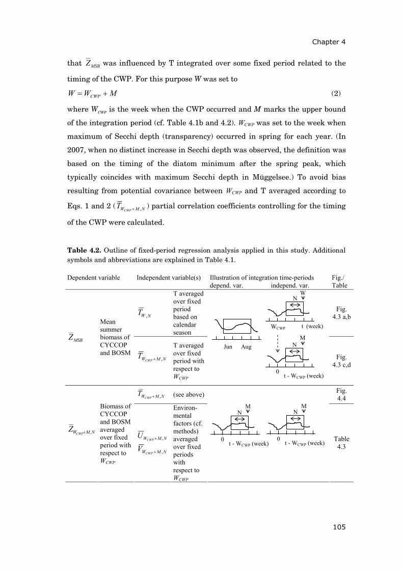
Chapter 4

105

that MSBZ was influenced by T integrated over some fixed period related to the

timing of the CWP. For this purpose W was set to

MWW CWP += (2)

where WCWP is the week when the CWP occurred and M marks the upper bound

of the integration period (cf. Table 4.1b and 4.2). WCWP was set to the week when

maximum of Secchi depth (transparency) occurred in spring for each year. (In

2007, when no distinct increase in Secchi depth was observed, the definition was

based on the timing of the diatom minimum after the spring peak, which

typically coincides with maximum Secchi depth in Müggelsee.) To avoid bias

resulting from potential covariance between WCWP and T averaged according to

Eqs. 1 and 2 ( NMWCWPT ,+ ) partial correlation coefficients controlling for the timing

of the CWP were calculated.

Table 4.2. Outline of fixed-period regression analysis applied in this study. Additional symbols and abbreviations are explained in Table 4.1. Dependent variable Independent variable(s) Illustration of integration time-periods depend. var. independ. var.

Fig./ Table

NWT ,

T averaged over fixed period based on calendar season

Fig. 4.3 a,b

MSBZ

Mean summer biomass of CYCCOP and BOSM

NMWCWPT ,+

T averaged over fixed period with respect to WCWP

Fig. 4.3 c,d

NMWCWPT ,+ (see above) Fig.

4.4

NMWCWPZ ,+

Biomass of CYCCOP and BOSM averaged over fixed period with respect to WCWP

NMWCWPU ,+

NMWCWPV ,+

Environ-mental factors (cf. methods) averaged over fixed periods with respect to WCWP

Table

4.3

t - WCWP (week)

t (week) WCWP

0

N M

N W

t - WCWP (week) 0

N M

Aug Jun

t - WCWP (week) 0

N M

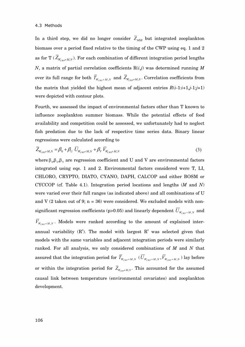
4.3 Methods

106

In a third step, we did no longer consider MSBZ but integrated zooplankton

biomass over a period fixed relative to the timing of the CWP using eq. 1 and 2

as for T ( NMWCWPZ ,+ ). For each combination of different integration period lengths

N, a matrix of partial correlation coefficients R(i,j) was determined running M

over its full range for both NMWCWPT ,+ and NMWCWP

Z ,+ . Correlation coefficients from

the matrix that yielded the highest mean of adjacent entries R(i-1:i+1,j-1:j+1)

were depicted with contour plots.

Fourth, we assessed the impact of environmental factors other than T known to

influence zooplankton summer biomass. While the potential effects of food

availability and competition could be assessed, we unfortunately had to neglect

fish predation due to the lack of respective time series data. Binary linear

regressions were calculated according to

NMWVNMWUNMW CWPCWPCWPVUZ ,,0, +++ ++= βββ (3)

where β0,βU,βV are regression coefficient and U and V are environmental factors

integrated using eqs. 1 and 2. Environmental factors considered were T, LI,

CHLORO, CRYPTO, DIATO, CYANO, DAPH, CALCOP and either BOSM or

CYCCOP (cf. Table 4.1). Integration period locations and lengths (M and N)

were varied over their full ranges (as indicated above) and all combinations of U

and V (2 taken out of 9; n = 36) were considered. We excluded models with non-

significant regression coefficients (p>0.05) and linearly dependent NMWCWPU ,+ and

NMWCWPV ,+ . Models were ranked according to the amount of explained inter-

annual variability (R2). The model with largest R2 was selected given that

models with the same variables and adjacent integration periods were similarly

ranked. For all analysis, we only considered combinations of M and N that

assured that the integration period for NMWCWPT ,+ ( NMWCWP

U ,+ , NMWCWPV ,+ ) lay before

or within the integration period for NMWCWPZ ,+ . This accounted for the assumed

causal link between temperature (environmental covariates) and zooplankton

development.

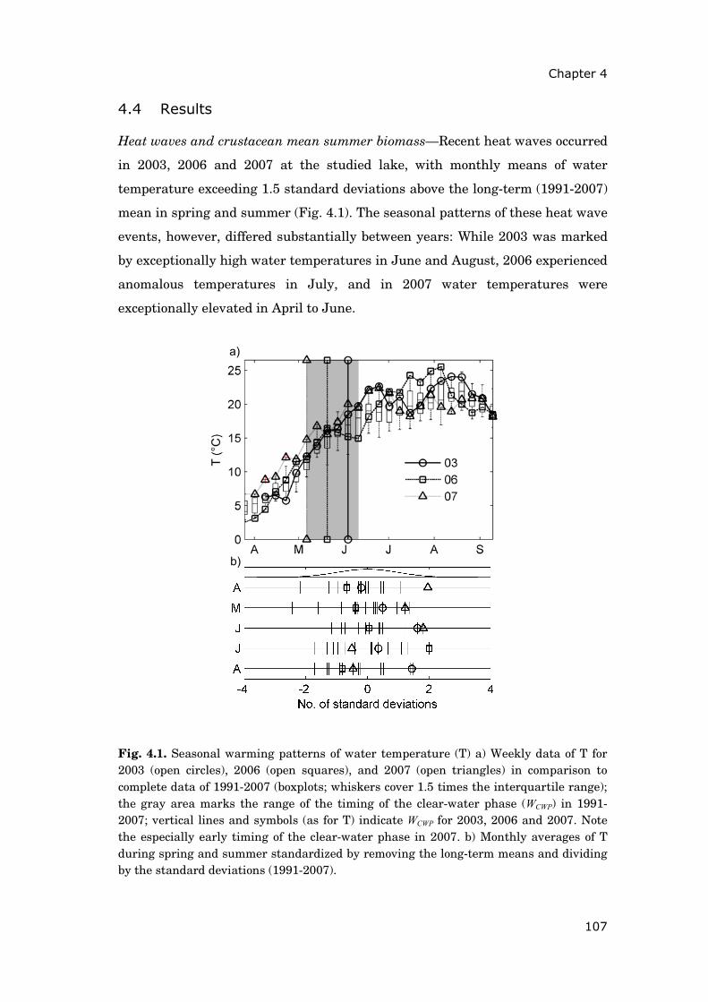
Chapter 4

107

4.4 Results

Heat waves and crustacean mean summer biomass—Recent heat waves occurred

in 2003, 2006 and 2007 at the studied lake, with monthly means of water

temperature exceeding 1.5 standard deviations above the long-term (1991-2007)

mean in spring and summer (Fig. 4.1). The seasonal patterns of these heat wave

events, however, differed substantially between years: While 2003 was marked

by exceptionally high water temperatures in June and August, 2006 experienced

anomalous temperatures in July, and in 2007 water temperatures were

exceptionally elevated in April to June.

Fig. 4.1. Seasonal warming patterns of water temperature (T) a) Weekly data of T for 2003 (open circles), 2006 (open squares), and 2007 (open triangles) in comparison to complete data of 1991-2007 (boxplots; whiskers cover 1.5 times the interquartile range); the gray area marks the range of the timing of the clear-water phase (WCWP) in 1991-2007; vertical lines and symbols (as for T) indicate WCWP for 2003, 2006 and 2007. Note the especially early timing of the clear-water phase in 2007. b) Monthly averages of T during spring and summer standardized by removing the long-term means and dividing by the standard deviations (1991-2007).

a)

b)

4.4 Results

108

Despite heat waves of similar average strength, mean summer biomass of total

crustacean zooplankton was exceptionally high in 2003 only (Fig. 4.2). It did not

show any outstanding development during the summer of 2006 and 2007. By

contrast, in 2003 a magnitude was reached that was last observed during the

hypertrophic phase of the lake, which was characterized by high phytoplankton

biovolume. The exceptional development of crustaceans in 2003 was largely due

to cyclopoid copepods and bosminids, which attained mean summer biomasses

( MSBZ ) that lay 2.8 and 2.2 standard deviations above their long-term means,

respectively (Fig. 4.2).

Fig. 4.2. Inter-annual variability of crustacean summer biomass during the hypertrophic (1980-1990) and eutrophic period (1991-2007) in Müggelsee: a) Deviations of crustacean mean summer biomass and phytoplankton mean summer biovolume from their long-term means (1980-2007); b) Mean summer biomass of main crustacean subgroups standardized by removing the long-term means and dividing by the standard deviations of the eutrophic period. Note the exceptionally high biomass of cyclopoid copepods and bosminids in 2003. Abbreviations as listed in Table 4.1.

a)

hypertrophic eutrophic

2003

b) 2003

Chapter 4

109

Next, we aimed to identify crucial time periods of elevated temperatures in the

long-term data (1991-2007) to examine our hypothesis that the heat wave

impact on cyclopoid copepods and bosminids was dependent on the temporal

patterning of its occurrence.

Temporal correlations between MSBZ and T—Interestingly, the crucial time

periods identified by correlation analysis (Table 4.2) were not fixed relative to

the calendar season but rather fixed relative to the timing of the CWP.

Correlation coefficients between water temperature integrated over a fixed

period between April and August ( NWT , ) and mean summer biomass ( MSBZ ) of

cyclopoid copepods and bosminids were relatively low (Fig. 4.3a,b). Marginally

significant (p<0.05) correlations were only found for cyclopoid copepods (Fig.

4.3a). In contrast, integrating T over a fixed period relative to the timing of the

CWP ( NMWCWPT ,+ ) resulted in significant (p<0.01) partial correlation coefficients

for both crustacean subgroups (Fig. 4.3c,d). Correlation coefficients suggested

that crucial time periods of elevated water temperature lay shortly after and

before the CWP for cyclopoid copepods and bosminids respectively.

Temporal correlations between NMWCWPZ ,+ and NMWCWP

T ,+ —When accounting for

the seasonal dynamics of crustaceans with respect to the timing of the CWP (i.e.

basing correlation analysis on NMWCWPZ ,+ ; Table 4.2), instead of considering mean

summer biomass, similar crucial time periods were identified. Mean start-up

population biomasses of cyclopoid copepods ( 5,7+CWPWZ ) and bosminids ( 3,6+CWPWZ ),

developing after the food bottleneck of the CWP, were most strongly correlated

with mean water temperature shortly after ( 2,3+CWPWT ) and before ( 2,2−CWPWT ) the

CWP, respectively (Fig. 4.4a,b; Fig. 4.5 gray areas I). These start-up populations

determined the success of cyclopoid copepods and bosminids throughout the

summer, as suggested by positive correlations with mean summer biomass (r =

0.62, p<0.01 for cyclopoid copepods and r = 0.78, p<0.001 for bosminids).

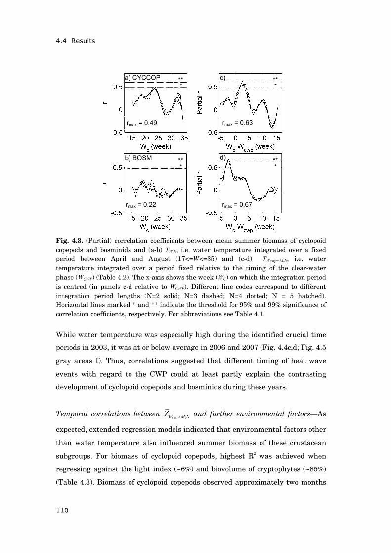
4.4 Results

110

Fig. 4.3. (Partial) correlation coefficients between mean summer biomass of cyclopoid copepods and bosminids and (a-b) TW,N, i.e. water temperature integrated over a fixed period between April and August (17<=W<=35) and (c-d) TWcwp+M,N, i.e. water temperature integrated over a period fixed relative to the timing of the clear-water phase (WCWP) (Table 4.2). The x-axis shows the week (WC) on which the integration period is centred (in panels c-d relative to WCWP). Different line codes correspond to different integration period lengths (N=2 solid; N=3 dashed; N=4 dotted; N = 5 hatched). Horizontal lines marked * and ** indicate the threshold for 95% and 99% significance of correlation coefficients, respectively. For abbreviations see Table 4.1.

While water temperature was especially high during the identified crucial time

periods in 2003, it was at or below average in 2006 and 2007 (Fig. 4.4c,d; Fig. 4.5

gray areas I). Thus, correlations suggested that different timing of heat wave

events with regard to the CWP could at least partly explain the contrasting

development of cyclopoid copepods and bosminids during these years.

Temporal correlations between NMWCWPZ ,+ and further environmental factors—As

expected, extended regression models indicated that environmental factors other

than water temperature also influenced summer biomass of these crustacean

subgroups. For biomass of cyclopoid copepods, highest R2 was achieved when

regressing against the light index (~6%) and biovolume of cryptophytes (~85%)

(Table 4.3). Biomass of cyclopoid copepods observed approximately two months

a) CYCCOP

rmax = 0.49 rmax = 0.63

b) BOSM

rmax = 0.22 rmax = 0.67

* c)

d)

**

* **

* **

* **

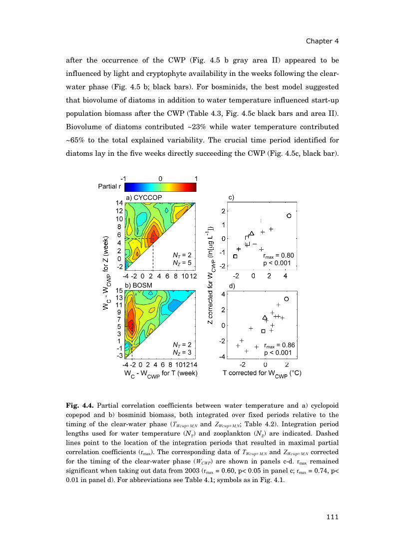
Chapter 4

111

after the occurrence of the CWP (Fig. 4.5 b gray area II) appeared to be

influenced by light and cryptophyte availability in the weeks following the clear-

water phase (Fig. 4.5 b; black bars). For bosminids, the best model suggested

that biovolume of diatoms in addition to water temperature influenced start-up

population biomass after the CWP (Table 4.3, Fig. 4.5c black bars and area II).

Biovolume of diatoms contributed ~23% while water temperature contributed

~65% to the total explained variability. The crucial time period identified for

diatoms lay in the five weeks directly succeeding the CWP (Fig. 4.5c, black bar).

Fig. 4.4. Partial correlation coefficients between water temperature and a) cyclopoid copepod and b) bosminid biomass, both integrated over fixed periods relative to the timing of the clear-water phase (TWcwp+M,N and ZWcwp+M,N; Table 4.2). Integration period lengths used for water temperature (NT) and zooplankton (NZ) are indicated. Dashed lines point to the location of the integration periods that resulted in maximal partial correlation coefficients (rmax). The corresponding data of TWcwp+M,N and ZWcwp+M,N corrected for the timing of the clear-water phase (WCWP) are shown in panels c-d. rmax remained significant when taking out data from 2003 (rmax = 0.60, p< 0.05 in panel c; rmax = 0.74, p< 0.01 in panel d). For abbreviations see Table 4.1; symbols as in Fig. 4.1.

NT = 2 NZ = 5

NT = 2 NZ = 3

rmax = 0.80 p < 0.001

rmax = 0.86 p < 0.001

c)

d) b) BOSM

a) CYCCOP

Partial r

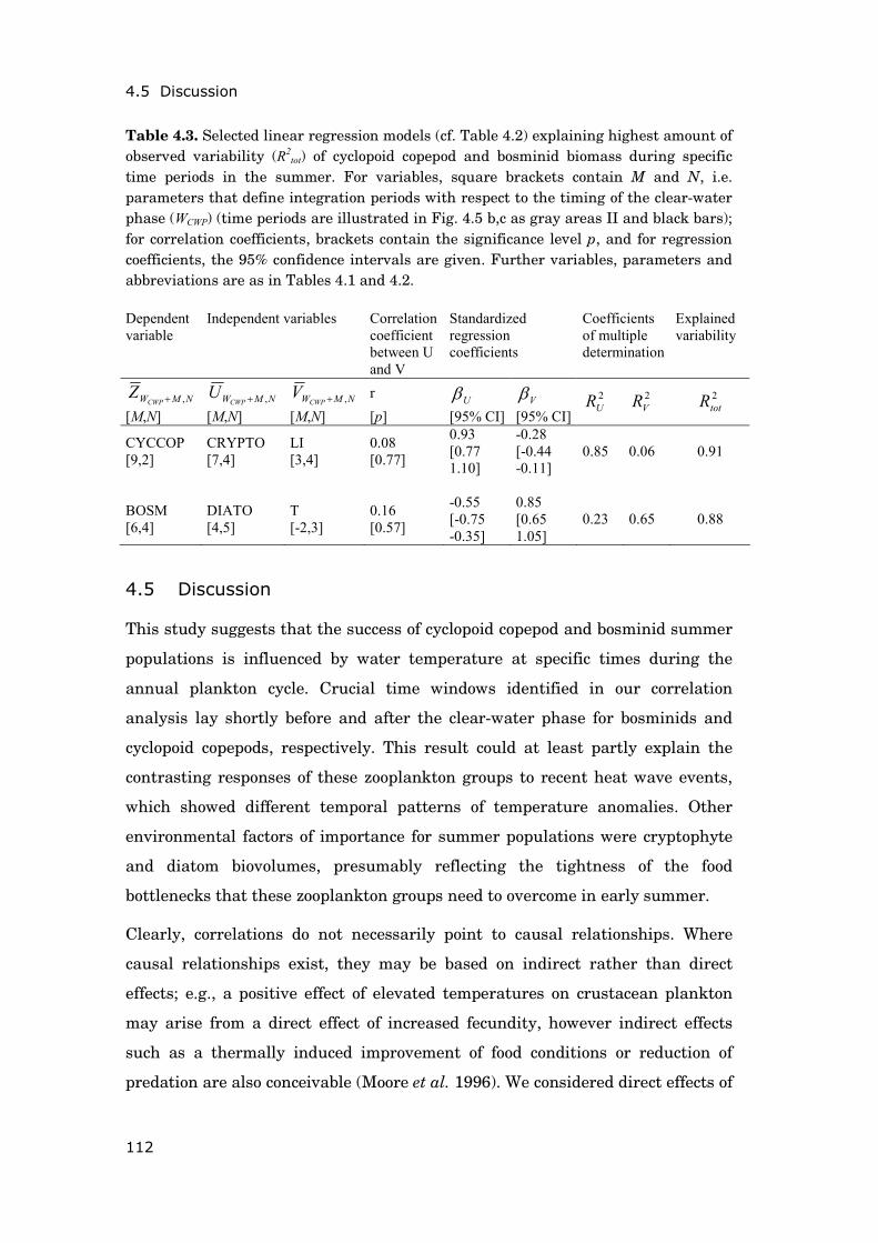
4.5 Discussion

112

Table 4.3. Selected linear regression models (cf. Table 4.2) explaining highest amount of observed variability (R2

tot) of cyclopoid copepod and bosminid biomass during specific time periods in the summer. For variables, square brackets contain M and N, i.e. parameters that define integration periods with respect to the timing of the clear-water phase (WCWP) (time periods are illustrated in Fig. 4.5 b,c as gray areas II and black bars); for correlation coefficients, brackets contain the significance level p, and for regression coefficients, the 95% confidence intervals are given. Further variables, parameters and abbreviations are as in Tables 4.1 and 4.2. Dependent variable

Independent variables Correlation coefficient between U and V

Standardized regression coefficients

Coefficients of multiple determination

Explained variability

NMWCWPZ ,+

[M,N] NMWCWP

U ,+

[M,N] NMWCWP

V ,+ [M,N]

r

[p] Uβ

[95% CI]Vβ

[95% CI]2

UR 2VR 2

totR

CYCCOP [9,2]

CRYPTO [7,4]

LI [3,4]

0.08 [0.77]

0.93 [0.77 1.10]

-0.28 [-0.44 -0.11]

0.85 0.06 0.91

BOSM [6,4]

DIATO [4,5]

T [-2,3]

0.16 [0.57]

-0.55 [-0.75 -0.35]

0.85 [0.65 1.05]

0.23 0.65 0.88

4.5 Discussion

This study suggests that the success of cyclopoid copepod and bosminid summer

populations is influenced by water temperature at specific times during the

annual plankton cycle. Crucial time windows identified in our correlation

analysis lay shortly before and after the clear-water phase for bosminids and

cyclopoid copepods, respectively. This result could at least partly explain the

contrasting responses of these zooplankton groups to recent heat wave events,

which showed different temporal patterns of temperature anomalies. Other

environmental factors of importance for summer populations were cryptophyte

and diatom biovolumes, presumably reflecting the tightness of the food

bottlenecks that these zooplankton groups need to overcome in early summer.

Clearly, correlations do not necessarily point to causal relationships. Where

causal relationships exist, they may be based on indirect rather than direct

effects; e.g., a positive effect of elevated temperatures on crustacean plankton

may arise from a direct effect of increased fecundity, however indirect effects

such as a thermally induced improvement of food conditions or reduction of

predation are also conceivable (Moore et al. 1996). We considered direct effects of

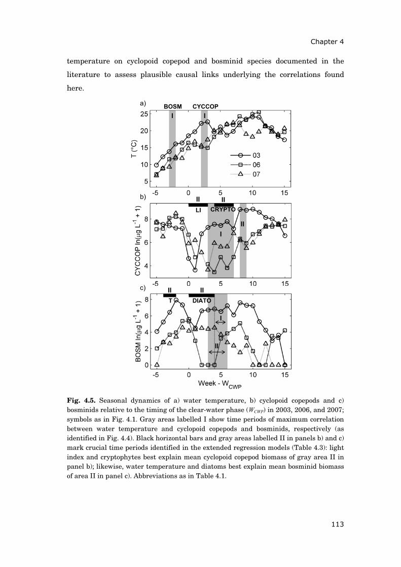
Chapter 4

113

temperature on cyclopoid copepod and bosminid species documented in the

literature to assess plausible causal links underlying the correlations found

here.

Fig. 4.5. Seasonal dynamics of a) water temperature, b) cyclopoid copepods and c) bosminids relative to the timing of the clear-water phase (WCWP) in 2003, 2006, and 2007; symbols as in Fig. 4.1. Gray areas labelled I show time periods of maximum correlation between water temperature and cyclopoid copepods and bosminids, respectively (as identified in Fig. 4.4). Black horizontal bars and gray areas labelled II in panels b) and c) mark crucial time periods identified in the extended regression models (Table 4.3): light index and cryptophytes best explain mean cyclopoid copepod biomass of gray area II in panel b); likewise, water temperature and diatoms best explain mean bosminid biomass of area II in panel c). Abbreviations as in Table 4.1.

BOSM CYCCOP

DIATOT

I

III

CRYPTOLI

a)

b)

c)

II

II II

II II

I I

4.5 Discussion

114

Potential mechanisms for the effect of water temperature on cyclopoid copepods—

A large number of laboratory studies have documented that increasing

temperatures accelerate the development times of eggs and larval stages

(nauplii and copepodids) of cyclopoid copepods (e.g., Vijverberg 1980; Maier

1989). The rate of emergence from diapause has also been shown to rise with

higher temperatures (Maier 1990). The question is a) how are these known

effects of temperature on demographic rates translated to elevated population

abundance and b) why is the timing shortly after the CWP crucial for this

putative process. Unfortunately, detailed data on eggs and larval stages of

cyclopoid copepods and emergence patterns are missing for the studied lake.

Nonetheless, we can deduce possible mechanisms from the literature and

supportive own investigations as follows:

The species that dominate cyclopoid copepod summer abundance in our lake

(Thermocyclops sp., Mesocyclops sp. and Acanthocyclops sp.) overwinter as late

copepodid stages in the sediment. Individuals are usually detected in the

pelagial zone for the first time in spring or early summer – in most cases before

the occurrence of the CWP (Gerten and Adrian 2002). The time when water

temperature surpasses 5-8°C (which usually takes place in April in Müggelsee)

has been shown to be a good predictor of the start of the pelagial phase of T.

oithonoides (Adrian et al. 2006). Interestingly, Hairston et al. (2000) have

suggested that cyclopoid copepods in contrast to cladocerans emerge from

resting stages at various times during the year. The species they investigated

(Mesocyclops edax and Acanthocyclops vernalis) showed patterns of emergence

with two peak times, in spring and in summer. We hypothesize that water

temperatures in the time period identified in this study (2-3 weeks after the

CWP; gray area I in Fig. 4.5a) could strongly influence the success of the

summer emergence from diapause, which presumably is initiated after the

CWP. The range of water temperature during this period encompasses between

below 15 °C to well above 20 °C in the three heat wave years (Fig. 4.5a). Maier

(1990) found different emergence rates of cyclopoid copepods (Mesocyclops

leuckarti and Thermocyclops crassus) for this temperature range: While at 20 °C

half of the individuals had emerged after a maximum of only 4 days, at 15°C it

took up to 25 days for 50% to leave diapause. A pulsed emergence of resting

Chapter 4

115

individuals during conditions that are favourable could increase survival

probabilities and ultimately translate to higher summer abundance of

copepodids and adults.

Besides temperature, light is discussed as an important cue for the termination

of diapause (e.g., Gyllström and Hansson 2004). It is conceivable that the period

of high water transparency during the CWP, allowing elevated light intensities

to reach the sediment of the lake, therefore plays a role in activating the

diapausing copepodids. Yet, our extended regression models contained a

negative coefficient for the light index suggesting a detrimental effect of high

light intensity shortly after the CWP on cyclopoid copepod abundance later in

the summer (Table 4.3; Fig. 4.5b). Since variability in water transparency is

mainly determined by phytoplankton abundance and composition in the lake

studied (Huber et al. 2008) we assume that this regression result does not reflect

a direct effect of light but rather an effect of food quantity and quality on

vulnerable stages of cyclopoid copepod development.

Nauplii are generally considered the bottleneck of cyclopoid copepod

development because they are particularly sensitive to poor food conditions

(Hopp and Maier 2005). Preferred food consists of small phytoplankton such as

cryptophytes and chlorophytes (Hansen and Santer 1995). In eutrophic lakes

such as Müggelsee these small algae are often the first to develop after the CWP

before they are replaced by larger algal species, which are less apt for nauplii

(Sommer et al. 1986). It has been suggested that faster development through the

vulnerable naupliar stage might reduce mortality (Seebens et al. 2007). This

phenomenon could represent another mechanism contributing to the positive

correlations between water temperature and summer biomass of cyclopoid

copepods found in this study. Naupliar development times have been shown to

strongly differ within the temperature range identified as crucial here: e.g.,

while M. leuckarti required ~26 days at 15°C to develop from the first naupliar

stage to the first copepodid stage, the time was approximately halved at 20°C

(Maier, 1989).

Additional evidence for the importance of nauplii food conditions stems from the

extended regression model (Table 4.3). Cryptophyte biomass was identified as a

4.5 Discussion

116

variable with surprisingly high explanatory force. Compatibly, the time-lag

between the centres of integration period for cryptophytes and cyclopoid

copepods was three weeks (Fig. 4.5b black bar and area II) which falls within

the range of naupliar development times identified by Maier (1989). Mean

cryptophyte biomass varied between 0.01 and 0.18 mg C L-1 in the identified

integration period. Since these values fall below typical food limitation

thresholds for cyclopoid copepod nauplii (such as 0.2 mg C L-1 for M. leuckarti

determined by Hansen and Santer 1995) cryptophyte availability might indeed

largely determine inter-annual differences in nauplii survival.

Potential mechanisms for the effect of water temperature on bosminids—Similar

to copepods, laboratory and field studies have shown that demographic rates

and emergence of bosminids directly depend on temperature (Allan 1977;

Vijverberg 1980; Vandekerkhove et al. 2005). These findings have been drawn

on to explain why elevated spring temperature commonly coincide with an

earlier growth onset and sometimes also an increased spring abundance of

bosminids in some lakes (Gerten and Adrian 2000; Straile and Adrian 2000).

However, considering the lagged response of bosminids to water temperature

found here (centres of integration periods with respect to the CWP (WC - WCWP)

were –2.5 weeks for water temperature and +5 weeks for bosminid biomass;

thus they lie > 7 weeks apart; Fig. 4.4 and 4.5) we assume that the correlations

observed most likely stem from indirect temperature effects possibly mediated

by changes in (i) food availability, (ii) competition among zooplankton or (iii)

predation pressure.

(i) The extended regression model included diatoms as the second most

important variable after water temperature to explain bosminids biomass

shortly after the CWP. At the same time, water temperature and diatoms as

included in the model were independent (Table 4.3), a finding that excludes any

indirect temperature effect mediated by diatoms. Bosminids are known to prefer

small phytoplankton for prey (DeMott and Kerfoot 1982) whereas the summer

diatom assemblage in Müggelsee consists of rather large species. Thus, the

negative effect of high diatom densities shortly after the CWP, as suggested by

the model, probably reflects unfavourable food conditions for bosminids under

Chapter 4

117

situations of high diatom abundance. (In fact, during the identified crucial time

period (weeks 0-4 after the CWP; cf. Table 4.3 and black bar DIATO in Fig. 4.5c)

average diatom biomass and the average contribution of cryptophytes and

chlorophytes to total phytoplankton biomass are negatively correlated r = -0.65,

p<0.01.)

(ii) Some studies have suggested that small bodied zooplankton such as

bosminids gain competitive advantage over larger bodied zooplankton at higher

temperatures (Moore et al. 1996). Thus, temperature driven changes in

competition among zooplankton might have contributed to the correlations

between spring water temperature and bosminid summer start-up populations.

Yet, all of the extended regression models that included negative coefficients for

daphnids, calanoid copepods or cyclopoid copepods (suggesting competition)

yielded lower explanatory power than the selected model (not shown).

(iii) Indirect temperature effects mediated by changes in predation have also

been documented for several cladoceran species, most prominently for fish

predation on daphnids (Moore et al. 1996; Wagner and Benndorf 2006). Due to

their smaller size bosminids are considered less vulnerable to fish predation

than daphnids (Hanazato and Yasuno 1989). However, accounting for the

possible effects of temperature driven changes in invertebrate predation on

bosminids would certainly be interesting to pursue in the future and could yield

a more direct explanation for the correlations with water temperature found

here.

Delayed responses of cladocerans and copepods to warming—

Parthenogenetically reproducing cladocerans have often been observed to

respond with shorter time-lags to warming than sexually reproducing copepods

undergoing more complex life cycles (Straile and Adrian 2000; Gerten and

Adrian 2002; Seebens et al. 2007) . By contrast, our results suggested that

copepods were influenced more promptly by periods of exceptionally elevated

water temperatures than bosminids. As discussed above it is most likely that

indirect effects of temperature on bosminids dominated over direct effects

explaining why we found longer time-lags than expected. Response time of

copepods on the other hand was probably determined by direct temperature

4.5 Discussion

118

effects here. In a recent study Wagner (2009) showed a direct effect of higher

water temperatures especially on thermophilic cyclopoid copepod species

abundances during extended periods of thermal stratification in Müggelsee.

Accounting for the clear-water phase to normalize phenology shifts—Normalizing

seasonal trajectories of variables by the timing of the CWP resulted in

significantly higher correlations than taking the more conventional approach of

sticking to the calendar season. The CWP has been shown to structure

crustacean seasonal dynamics, representing a period of extremely low food

availability for many species (Sommer et al. 1986). Slight changes in its timing

are often accompanied by synchronous phenology shifts of crustacean

populations. Therefore, by correcting for the timing of the CWP these phenology

shifts no longer blur strong links to typical patterns of plankton succession.

Accounting for important events in the annual cycle of lake ecosystems rather

than relating strictly to the calendar seasons has been successfully applied in

various other analyses of plankton time-series (Tirok and Gaedke, 2006;

Shatwell et al. 2008; Wagner and Adrian, 2009).

In our study, this change in perspective (Fig. 4.6) provided some explanation for

the contrasting responses of cyclopoid copepods and bosminid summer

populations to recent heat wave events. As an illustrative example, considering

the calendar season only (Fig. 4.3a; Fig. 4.6a) one might have expected a positive

effect of elevated water temperatures in June of 2003 and 2007 on the summer

abundance of cyclopoid copepods in both years. Accounting for the timing of the

CWP (Fig. 4.3c; Fig. 4.6b) yielded a considerably better explanation for the

differences in abundance observed (Fig. 4.2): while in 2003 water temperatures

were high shortly after the CWP, the period identified as crucial for cyclopoid

copepods, no such anomalies were observed in 2007. The temporal patterns of

warming with respect to the timing of the CWP (Fig. 4.6b) differed strongly

between 2003 and 2007 mainly because the CWP occurred exceptionally early in

2007 (Fig. 4.6a). This in turn can be related to an extremely warm spring (Fig.

4.1; Fig. 4.6a) that – as has been shown for Müggelsee and many freshwater

systems (Gerten and Adrian, 2000; Straile, 2002) – generally results in a

seasonal forward shift of the CWP.

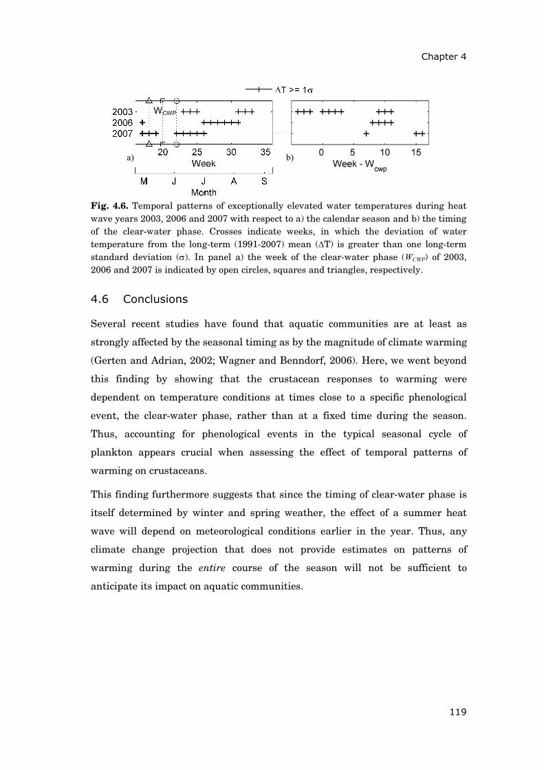
Chapter 4

119

Fig. 4.6. Temporal patterns of exceptionally elevated water temperatures during heat wave years 2003, 2006 and 2007 with respect to a) the calendar season and b) the timing of the clear-water phase. Crosses indicate weeks, in which the deviation of water temperature from the long-term (1991-2007) mean (ΔT) is greater than one long-term standard deviation (σ). In panel a) the week of the clear-water phase (WCWP) of 2003, 2006 and 2007 is indicated by open circles, squares and triangles, respectively.

4.6 Conclusions

Several recent studies have found that aquatic communities are at least as

strongly affected by the seasonal timing as by the magnitude of climate warming

(Gerten and Adrian, 2002; Wagner and Benndorf, 2006). Here, we went beyond

this finding by showing that the crustacean responses to warming were

dependent on temperature conditions at times close to a specific phenological

event, the clear-water phase, rather than at a fixed time during the season.

Thus, accounting for phenological events in the typical seasonal cycle of

plankton appears crucial when assessing the effect of temporal patterns of

warming on crustaceans.

This finding furthermore suggests that since the timing of clear-water phase is

itself determined by winter and spring weather, the effect of a summer heat

wave will depend on meteorological conditions earlier in the year. Thus, any

climate change projection that does not provide estimates on patterns of

warming during the entire course of the season will not be sufficient to

anticipate its impact on aquatic communities.

WCWP

a) b)

4.7 Acknowledgements

120

4.7 Acknowledgements

We thank all scientists and technicians who have been involved in the collection

and compilation of the long-term data set of Müggelsee. The study profited from

continuous discussions with Carola Wagner. The German Research Foundation

(DFG) supported Veronika Huber within the priority program AQUASHIFT

(Ad91/12-1).

General discussion

121

General discussion

The results presented in this thesis add to the growing body of evidence that

aquatic ecosystems have strongly responded to climatic changes of recent

decades. Given that past temperature rise has been small in comparison to

increases projected for the future (IPCC 2007) aquatic ecosystems will certainly

continue to be affected. What do the main findings of this thesis contribute to

better anticipate the changes in plankton growth patterns to be expected? How

could some of the analyses be carried on to further improve the required

understanding?

5.1 Modelling phytoplankton spring phenology Models presented in chapters 1 and 2 both indicated that an earlier onset of the

growing period due to climate change advances the spring phenology of

phytoplankton, in accordance with a large number of previous, mostly

observational studies (e.g., Weyhenmeyer et al. 1999; Gerten and Adrian 2000;

Adrian et al. 2006). The modeling approaches allowed gaining some insights into

the mechanisms that drive the observed forward shifts, albeit they suggested

differing mechanisms.

The detailed process-based model applied in chapter 1 indicated that high

winter and spring temperatures induced an earlier onset of diatom growth

because early ice-off provided sufficient light to reach the water column. Silicate

limitation then triggered the seasonal advancement of the bloom collapse

because silicate concentration was earlier drawn to its limitation threshold (a

mechanism also proposed recently by Meis et al. 2009). The bloom collapse also

occurred earlier in years in which it was caused by grazing because Daphnia

generally advanced their onset of growth similarly to diatoms after a warm

winter and spring.

The general and more simplified model approach applied in chapter 2 on the

other hand predicted an advancement of spring phenology through increased

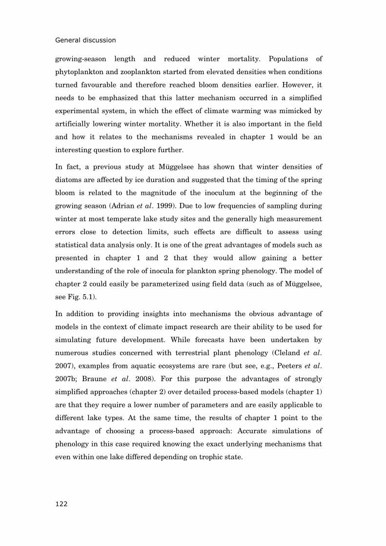
General discussion

122

growing-season length and reduced winter mortality. Populations of

phytoplankton and zooplankton started from elevated densities when conditions

turned favourable and therefore reached bloom densities earlier. However, it

needs to be emphasized that this latter mechanism occurred in a simplified

experimental system, in which the effect of climate warming was mimicked by

artificially lowering winter mortality. Whether it is also important in the field

and how it relates to the mechanisms revealed in chapter 1 would be an

interesting question to explore further.

In fact, a previous study at Müggelsee has shown that winter densities of

diatoms are affected by ice duration and suggested that the timing of the spring

bloom is related to the magnitude of the inoculum at the beginning of the

growing season (Adrian et al. 1999). Due to low frequencies of sampling during

winter at most temperate lake study sites and the generally high measurement

errors close to detection limits, such effects are difficult to assess using

statistical data analysis only. It is one of the great advantages of models such as

presented in chapter 1 and 2 that they would allow gaining a better

understanding of the role of inocula for plankton spring phenology. The model of

chapter 2 could easily be parameterized using field data (such as of Müggelsee,

see Fig. 5.1).

In addition to providing insights into mechanisms the obvious advantage of

models in the context of climate impact research are their ability to be used for

simulating future development. While forecasts have been undertaken by

numerous studies concerned with terrestrial plant phenology (Cleland et al.

2007), examples from aquatic ecosystems are rare (but see, e.g., Peeters et al.

2007b; Braune et al. 2008). For this purpose the advantages of strongly

simplified approaches (chapter 2) over detailed process-based models (chapter 1)

are that they require a lower number of parameters and are easily applicable to

different lake types. At the same time, the results of chapter 1 point to the

advantage of choosing a process-based approach: Accurate simulations of

phenology in this case required knowing the exact underlying mechanisms that

even within one lake differed depending on trophic state.

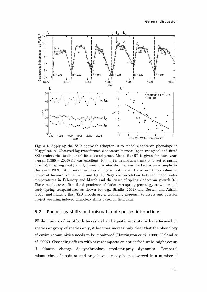
General discussion

123

Fig. 5.1. Applying the SSD approach (chapter 2) to model cladoceran phenology in Müggelsee. A) Observed log-transformed cladoceran biomass (open triangles) and fitted SSD trajectories (solid lines) for selected years. Model fit (R2) is given for each year; overall (1980 – 2006) fit was excellent: R2 = 0.79. Transition times t0 (onset of spring growth), tz (spring peak) and tφ (onset of winter decline) are marked as an example for the year 1989. B) Inter-annual variability in estimated transition times (showing temporal forward shifts in t0 and tz). C) Negative correlation between mean water temperatures in February and March and the onset of spring cladoceran growth (t0). These results re-confirm the dependence of cladoceran spring phenology on winter and early spring temperatures as shown by, e.g., Straile (2002) and Gerten and Adrian (2000) and indicate that SSD models are a promising approach to assess and possibly project warming induced phenology shifts based on field data.

5.2 Phenology shifts and mismatch of species interactions

While many studies of both terrestrial and aquatic ecosystems have focused on

species or group of species only, it becomes increasingly clear that the phenology

of entire communities needs to be monitored (Harrington et al. 1999; Cleland et

al. 2007). Cascading effects with severe impacts on entire food webs might occur,

if climate change de-synchronizes predator-prey dynamics. Temporal

mismatches of predator and prey have already been observed in a number of

Spearman‘s r = - 0.69 p < 0.001

t0

tz

tΦ

B C

tz tΦ A t0

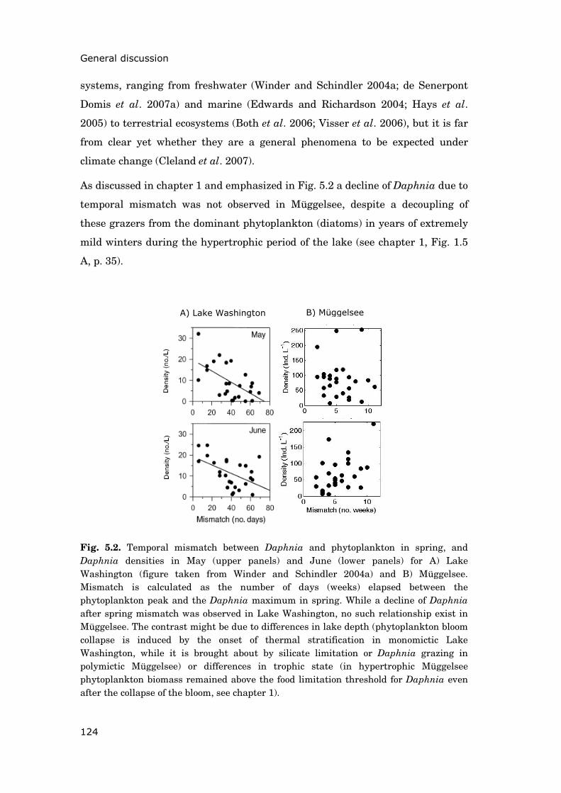
General discussion

124

systems, ranging from freshwater (Winder and Schindler 2004a; de Senerpont

Domis et al. 2007a) and marine (Edwards and Richardson 2004; Hays et al.

2005) to terrestrial ecosystems (Both et al. 2006; Visser et al. 2006), but it is far

from clear yet whether they are a general phenomena to be expected under

climate change (Cleland et al. 2007).

As discussed in chapter 1 and emphasized in Fig. 5.2 a decline of Daphnia due to

temporal mismatch was not observed in Müggelsee, despite a decoupling of

these grazers from the dominant phytoplankton (diatoms) in years of extremely

mild winters during the hypertrophic period of the lake (see chapter 1, Fig. 1.5

A, p. 35).

Fig. 5.2. Temporal mismatch between Daphnia and phytoplankton in spring, and Daphnia densities in May (upper panels) and June (lower panels) for A) Lake Washington (figure taken from Winder and Schindler 2004a) and B) Müggelsee. Mismatch is calculated as the number of days (weeks) elapsed between the phytoplankton peak and the Daphnia maximum in spring. While a decline of Daphnia after spring mismatch was observed in Lake Washington, no such relationship exist in Müggelsee. The contrast might be due to differences in lake depth (phytoplankton bloom collapse is induced by the onset of thermal stratification in monomictic Lake Washington, while it is brought about by silicate limitation or Daphnia grazing in polymictic Müggelsee) or differences in trophic state (in hypertrophic Müggelsee phytoplankton biomass remained above the food limitation threshold for Daphnia even after the collapse of the bloom, see chapter 1).

A) Lake Washington B) Müggelsee

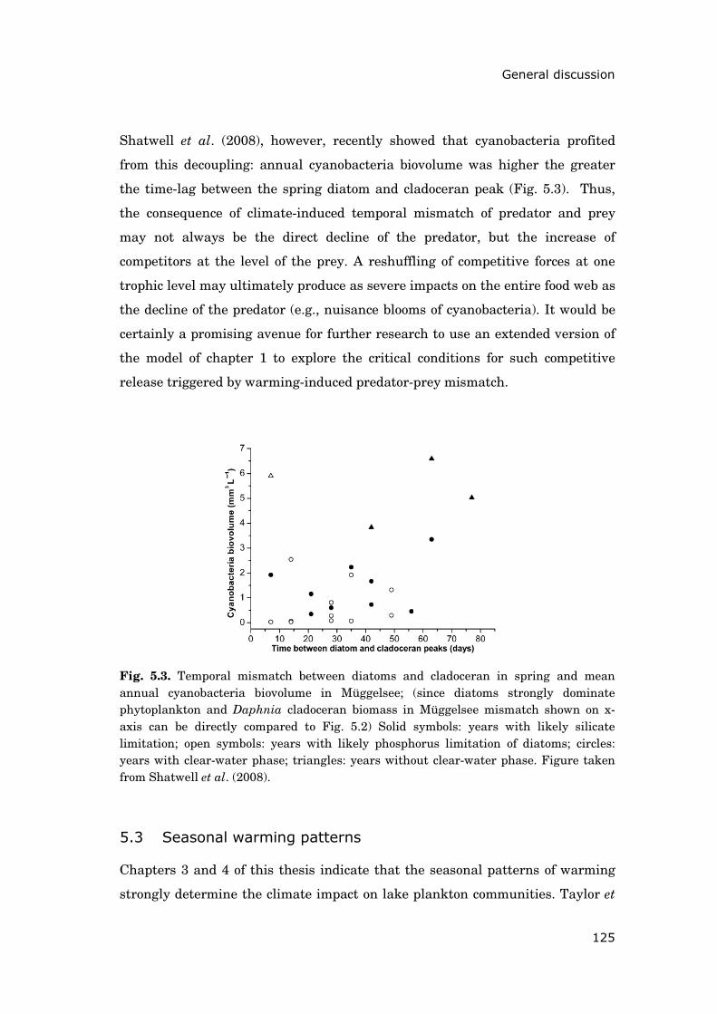
General discussion

125

Shatwell et al. (2008), however, recently showed that cyanobacteria profited

from this decoupling: annual cyanobacteria biovolume was higher the greater

the time-lag between the spring diatom and cladoceran peak (Fig. 5.3). Thus,

the consequence of climate-induced temporal mismatch of predator and prey

may not always be the direct decline of the predator, but the increase of

competitors at the level of the prey. A reshuffling of competitive forces at one

trophic level may ultimately produce as severe impacts on the entire food web as

the decline of the predator (e.g., nuisance blooms of cyanobacteria). It would be

certainly a promising avenue for further research to use an extended version of

the model of chapter 1 to explore the critical conditions for such competitive

release triggered by warming-induced predator-prey mismatch.

Fig. 5.3. Temporal mismatch between diatoms and cladoceran in spring and mean annual cyanobacteria biovolume in Müggelsee; (since diatoms strongly dominate phytoplankton and Daphnia cladoceran biomass in Müggelsee mismatch shown on x-axis can be directly compared to Fig. 5.2) Solid symbols: years with likely silicate limitation; open symbols: years with likely phosphorus limitation of diatoms; circles: years with clear-water phase; triangles: years without clear-water phase. Figure taken from Shatwell et al. (2008).

5.3 Seasonal warming patterns

Chapters 3 and 4 of this thesis indicate that the seasonal patterns of warming

strongly determine the climate impact on lake plankton communities. Taylor et

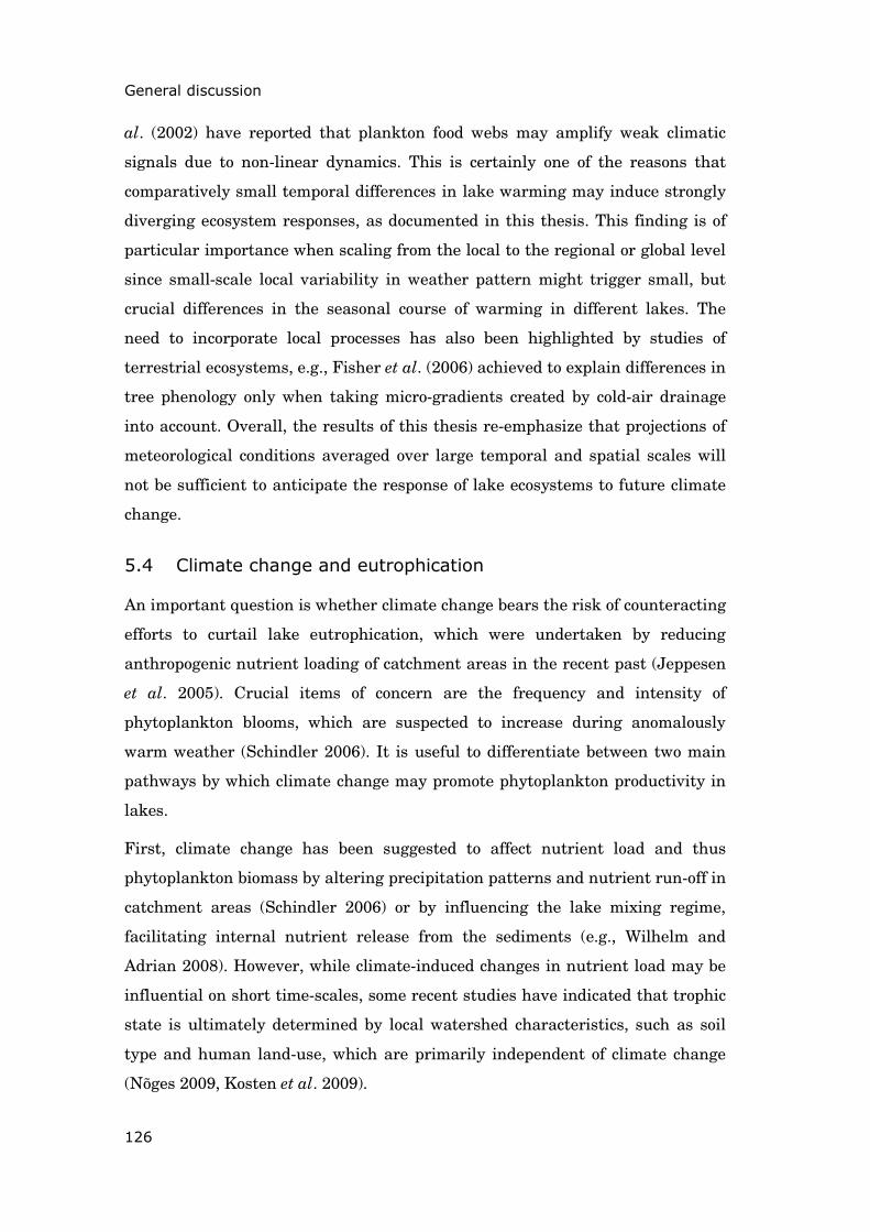
General discussion

126

al. (2002) have reported that plankton food webs may amplify weak climatic

signals due to non-linear dynamics. This is certainly one of the reasons that

comparatively small temporal differences in lake warming may induce strongly

diverging ecosystem responses, as documented in this thesis. This finding is of

particular importance when scaling from the local to the regional or global level

since small-scale local variability in weather pattern might trigger small, but

crucial differences in the seasonal course of warming in different lakes. The

need to incorporate local processes has also been highlighted by studies of

terrestrial ecosystems, e.g., Fisher et al. (2006) achieved to explain differences in

tree phenology only when taking micro-gradients created by cold-air drainage

into account. Overall, the results of this thesis re-emphasize that projections of

meteorological conditions averaged over large temporal and spatial scales will

not be sufficient to anticipate the response of lake ecosystems to future climate

change.

5.4 Climate change and eutrophication

An important question is whether climate change bears the risk of counteracting

efforts to curtail lake eutrophication, which were undertaken by reducing

anthropogenic nutrient loading of catchment areas in the recent past (Jeppesen

et al. 2005). Crucial items of concern are the frequency and intensity of

phytoplankton blooms, which are suspected to increase during anomalously

warm weather (Schindler 2006). It is useful to differentiate between two main

pathways by which climate change may promote phytoplankton productivity in

lakes.

First, climate change has been suggested to affect nutrient load and thus

phytoplankton biomass by altering precipitation patterns and nutrient run-off in

catchment areas (Schindler 2006) or by influencing the lake mixing regime,

facilitating internal nutrient release from the sediments (e.g., Wilhelm and

Adrian 2008). However, while climate-induced changes in nutrient load may be

influential on short time-scales, some recent studies have indicated that trophic

state is ultimately determined by local watershed characteristics, such as soil

type and human land-use, which are primarily independent of climate change

(Nõges 2009, Kosten et al. 2009).

General discussion

127

Second, climate-induced change in water temperature, incident radiation, ice

cover, and thermal stratification exert direct effects on phytoplankton growth

and may thereby impact on the magnitude of phytoplankton blooms. For

example, a recent study on re-oligotrophication of Lake Geneva suggested an

increase in primary production and phytoplankton biomass despite falling

nutrient concentrations due to higher availability of light and strengthened

thermal stratification (Tadonleke et al. 2009). However, other studies have

found that warming may exacerbate some symptoms of eutrophication such as

de-oxygenation and reduced fish biomass (Feuchtmayr et al. 2009) or may

influence the temporal organization and vertical positioning of the

phytoplankton community (Winder and Hunter 2009), but did not affect total

phytoplankton biomass. Sommer and Lengfellner (2008) have even reported that

in their mesocosm experiments temperature elevation decreased phytoplankton

peak biomass in spring. They speculated that in warmer mesocosms higher

grazer activity lowered accumulation of phytoplankton biomass during the

spring bloom.

In the light of these findings, which conclusions can be drawn from the results of

this thesis? In chapter 1, I modelled trophic state independently of climate

change by imposing a maximum amount of available phosphorus regardless of

meteorological conditions. Making the phosphorus recycling rate (see chapter 1,

eq. 3) dependent on temperature would be an interesting extension to the model,

allowing for better differentiating between direct climate impacts on

phytoplankton via water temperature and ice-cover and more indirect effects via

potentially accelerated phosphorus recycling. In the simulation experiments

applied, climatic conditions (water temperature and ice cover) only slightly

modified the magnitude of the diatom spring bloom, which was predetermined

by the lake’s trophic state (phosphorus availability) (see chapter 1, Fig. 1.3, p.

33). Thus, with the mentioned caveats, the findings of chapter 1 suggest that,

regarding the magnitude of the phytoplankton blooms in spring, climate change

is unlikely to fully counteract successfully implemented nutrient reduction

measures of recent decades.

In contrast, results of chapter 3 suggest that extreme meteorological conditions

in the summer can principally work against past containment of eutrophication

General discussion

128

by favouring cyanobacteria, which profit from intensified thermal stratification.

However, whether increased cyanobacteria dominance during heat waves will

remain an exception or will become a general rule in the future, will not only

depend on the frequency of heat waves but also on their seasonal timing and

duration, and food web interactions, as I have also shown in chapter 3. Yet, it is

important to note that these conclusions apply only to moderately eutrophic,

polymictic lakes: Wagner and Adrian (2009) found that under hypertrophic

conditions, characterized by extremely high total phosphorus concentrations,

dominance of cyanobacteria is promoted independently of the thermal regime.

Overall, the findings of this thesis suggest that nutrients remain the primary

agents determining the magnitude of phytoplankton blooms, but that future

climate change may exacerbate symptoms of eutrophication, such as the

occurrence of cyanobacteria blooms. My results also indicate that the impacts of

climate change (concerning timing and magnitude of phytoplankton blooms) in

nutrient-rich lakes are more severe than in nutrient-poor lakes. Consequently,

lake management that aims at containing eutrophication by reducing the

anthropogenic supply of phosphorus and nitrogen to watersheds remains

essential and might under future global warming prove even more important

than in the past.

5.5 Conclusions

This thesis contributes to a better mechanistic understanding of the climate

impacts on the timing and magnitude of phytoplankton blooms in shallow lakes.

Key conclusions regarding the overarching research questions (see section 0.2,

Fig. 0.4, p. 11) are:

(1) Trophic state determines the mechanisms that drive phytoplankton

spring phenology in shallow lakes. Eutrophication amplifies the temporal

advancement of the phytoplankton spring bloom triggered by climate

warming.

(2) Future climate change is likely to further advance phytoplankton spring

blooming in the season. However, accurately projecting spring phenology

of phytoplankton may prove more demanding than of terrestrial plants,

General discussion

129

since in addition to meteorological conditions food web interactions and

especially nutrient availability and will need to be accounted for.

(3) The risk of decoupling the phytoplankton from the zooplankton spring

peak due to de-synchronized phenology shifts is more elevated in

nutrient-rich than in nutrient-poor shallow lakes. The consequence of

predator-prey mismatch in nutrient-rich systems is not necessarily a

decline of the predator.

(4) Summer heat waves do not generally promote cyanobacteria in eutrophic,

polymictic lakes. Their seasonal timing and duration determine whether

critical thresholds of thermal stratification, decisive for cyanobacteria

bloom formation, are crossed.

(5) The temporal patterns of heat wave events critically influence the

summer abundance of some zooplankton species, which may serve as a

buffer by suppressing phytoplankton bloom formation.

(6) Nutrients are the primary drivers of phytoplankton bloom magnitudes.

However, future climate warming has the potential to exacerbate some

symptoms of eutrophication, such as the occurrence of cyanobacteria

blooms.

130

References

131

References

Adrian R. & Frost T.M. (1992). Comparative feeding ecology of Tropocyclops-

prasinus-mexicanus (Copepoda, Cyclopoida). Journal of Plankton

Research, 14, 1369-1382.

Adrian R., Walz N., Hintze T., Hoeg S. & Rusche R. (1999). Effects of ice

duration on plankton succession during spring in a shallow polymictic

lake. Freshwater Biology, 41, 621-632.

Adrian R. & Hintze T. (2000). Effects of winter air temperature on the ice

phenology of the Müggelsee (Berlin, Germany). Verh. Internat. Verein.

Limnol., 27, 2808-2811.

Adrian R., Wilhelm S. & Gerten D. (2006). Life-history traits of lake plankton

species may govern their phenological response to climate warming.

Global Change Biology, 12, 652-661.

Adrian R., O’Reilly C.M., Zagarese H., et al. (2009) Lakes as sentinels of climate

change. Limnology and Oceanography, 54, in press.

Allan J.D. (1977). Analysis of seasonal dynamics of a mixed population of

Daphnia, and associated cladoceran community. Freshwater Biology, 7,

505-512.

Allen J.I., Howland R.M.H., Bloomer N. & Uncles R.J. (1998). Simulating the

spring phytoplankton bloom in the Humber plume, UK. Marine Pollution

Bulletin, 37, 295-305.

Andersen T. (1997). Pelagic nutrient cycles: herbivores as sources and sinks.

Springer Verlag, Heidelberg.

Arhonditsis G.B. & Brett M.T. (2005). Eutrophication model for Lake

Washington (USA) Part I. Model description and sensitivity analysis.

Ecological Modelling, 187, 140-178.

Battisti D.S. & Naylor R.L. (2009). Historical Warnings of Future Food

Insecurity with Unprecedented Seasonal Heat. Science, 323, 240-244.

Benndorf J., Kranich J., Mehner T. & Wagner A. (2001). Temperature impact on

the midsummer decline of Daphnia galeata: an analysis of long-term data

References

132

from the biomanipulated Bautzen Reservoir (Germany). Freshwater

Biology, 46, 199-211.

Berger S.A., Diehl S., Stibor H., Trommer G., Ruhenstroth M., Wild A., Weigert

A., Jäger C.G. & Striebel M. (2007). Water temperature and mixing

depth affect timing and magnitude of events during spring succession of

the plankton. Oecologia, 150, 643-654.

Blenckner T., Adrian R., Livingstone D.M., Jennings E., Weyhenmeyer G.A.,

George D.G., Jankowski T., Jarvinen M., Aonghusa C.N., Noges T.,

Straile D. & Teubner K. (2007). Large-scale climatic signatures in lakes

across Europe: a meta-analysis. Global Change Biology, 13, 1314-1326.

Both C., Bouwhuis S., Lessells C.M. & Visser M.E. (2006). Climate change and

population declines in a long-distance migratory bird. Nature, 441, 81-83.

Bottrell H.H., Duncan A., Gliwicz Z.M., Grygierek E., Herzig A.,

Hillbrichtilkowska A., Kurasawa H., Larsson P. & Weglenska T. (1976).

Review of some problems in zooplankton production studies. Norwegian

Journal of Zoology, 24, 419-456.

Bowie, G.L., W.B. Mills, D.B. Porcella, C.L. Campbell, J.R. Pagenkopf, G.L.

Rupp, K.M. Johnson, P.W.H. Chan, and S.A. Gherini. 1985. Rates,

constants, and kinetics formulations in surface water quality modelling.

EPA/600/3-85/040, 2nd ed., U.S. Environmental Protection Agency.

Braune E., Richter O., Sondgerath D. & Suhling F. (2008). Voltinism flexibility

of a riverine dragonfly along thermal gradients. Global Change Biology,

14, 470-482.

Breiman L., Friedman J., Stone C.J. & Olshen R.A. (1993). Classification and

regression trees. Chapman & Hall, Boca Raton.

Burns C.W. (1968). Relationship between body size of filter-feeding cladocera

and maximum size of particle ingested. Limnology and Oceanography,

13, 675-678.

Butterwick C., Heaney S.I. & Talling J.F. (2005). Diversity in the influence of

temperature on the growth rates of freshwater algae, and its ecological

relevance. Freshwater Biology, 50, 291-300.

Caceres C.E. (1998). Interspecific variation in the abundance, production, and

emergence of Daphnia diapausing eggs. Ecology, 79, 1699-1710.

References

133

Chan F., Pace M.L., Howarth R.W. & Marino R.M. (2004). Bloom formation in

heterocystic nitrogen-fixing cyanobacteria: The dependence on colony size

and zooplankton grazing. Limnology and Oceanography, 49, 2171-2178.

Chen C.Y. & Folt C.L. (2002). Ecophysiological responses to warming events by

two sympatric zooplankton species. Journal of Plankton Research, 24,

579-589.

Chorus I. & Bartram J. (1999). Toxic Cyanobacteria in Water: A Guide to their

Public Health Consequences, Monitoring and Management. Spon,

London.

Cleland E.E., Chuine I., Menzel A., Mooney H.A. & Schwartz M.D. (2007).

Shifting plant phenology in response to global change. Trends in Ecology

& Evolution, 22, 357-365.

Conley D.J., Schelske C.L. & Stoermer E.F. (1993). Modification of the

biogeochemical cycle of silica with eutrophication. Marine Ecology-

Progress Series, 101, 179-192.

Daufresne M., Bady P. & Fruget J.F. (2007). Impacts of global changes and

extreme hydroclimatic events on macroinvertebrate community

structures in the French Rhone River. Oecologia, 151, 544-559.

Davidowicz P.Z., Gliwicz M. & Gulati R.D. (1988). Can Daphnia prevent a blue-

green algae bloom in hypertrophic lakes? Limnologica, 19, 21-26.

De Senerpont Domis L.N.D., Mooij W.M. & Huisman J. (2007a). Climate-

induced shifts in an experimental phytoplankton community: a

mechanistic approach. Hydrobiologia, 584, 403-413.

De Senerpont Domis L.N.D., Mooij W.M., Hulsmann S., van Nes E.H. & Scheffer

M. (2007b). Can overwintering versus diapausing strategy in Daphnia

determine match-mismatch events in zooplankton-algae interactions?

Oecologia, 150, 682-698.

Demott W.R. & Kerfoot W.C. (1982). Competition among cladocerans – nature of

interaction between Bosmina and Daphnia. Ecology, 63, 1949-1966.

Diehl S., Berger S. & Wöhrl R. (2005). Flexible nutrient stoichiometry mediates

environmental influences, on phytoplankton and its resources. Ecology,

86, 2931-2945.

Dokulil M.T. & Teubner K. (2000). Cyanobacterial dominance in lakes.

References

134

Hydrobiologia, 438, 1-12.

Downing J.A., Watson S.B. & McCauley E. (2001). Predicting Cyanobacteria

dominance in lakes. Canadian Journal of Fisheries and Aquatic Sciences,

58, 1905-1908.

Driescher E., Behrendt H., Schellenberger G. & Stellmacher R. (1993). Lake

Müggelsee and ist environment – natural conditions and anthropogenic

impacts. Internationale Revue der Gesamten Hydrobiologie, 78, 327-343.

Droop M.R. (1983). 25 years of algal growth kinetics – a personal view. Botanica

Marina, 26, 99-112.

Edwards M. & Richardson A.J. (2004). Impact of climate change on marine

pelagic phenology and trophic mismatch. Nature, 430, 881-884.

Elliott J.A., Jones I.D. & Thackeray S.J. (2006). Testing the sensitivity of

phytoplankton communities to changes in water temperature and

nutrient load, in a temperate lake. Hydrobiologia, 559, 401-411.

Feuchtmayr H., Moran R., Hatton K., Connor L., Heyes T., Moss B., Harvey I. &

Atkinson D. (2009). Global warming and eutrophication: effects on water

chemistry and autotrophic communities in experimental hypertrophic

shallow lake mesocosms. Journal of Applied Ecology, 46, 713-723.

Fisher J.I., Mustard J.F. & Vadeboncoeur M.A. (2006). Green leaf phenology at

Landsat resolution: Scaling from the field to the satellite. Remote Sensing

of Environment, 100, 265-279.

Gerten D. & Adrian R. (2000). Climate-driven changes in spring plankton

dynamics and the sensitivity of shallow polymictic lakes to the North

Atlantic Oscillation. Limnology and Oceanography, 45, 1058-1066.

Gerten D. & Adrian R. (2002). Species-specific changes in the phenology and

peak abundance of freshwater copepods in response to warm summers.

Freshwater Biology, 47, 2163-2173.

Giebelhausen B. & Lampert W. (2001). Temperature reaction norms of Daphnia

magna: the effect of food concentration. Freshwater Biology, 46, 281-289.

Gleick P.H. (1996). Water resources. In: Encyclopedia of Climate and Weather,

(ed.) Schneider S.H., Oxford University Press, New York.

Gyllstrom M. & Hansson L.A. (2004). Dormancy in freshwater zooplankton:

Induction, termination and the importance of benthic-pelagic coupling.

References

135

Aquatic Sciences, 66, 274-295.

Hairston N.G., Hansen A.M. & Schaffner W.R. (2000). The effect of diapause

emergence on the seasonal dynamics of a zooplankton assemblage.

Freshwater Biology, 45, 133-145.

Hanazato T. & Yasuno M. (1989). Zooplankton community structure driven by

vertebrate and invertebrate predators. Oecologia, 81, 450-458.

Hansen A.M. & Santer B. (1995). The influence of food resources on the

development, survival and reproduction of the 2 cyclopoid copepods

Cyclops vicinus and Mesocyclops leuckarti. Journal of Plankton Research,

17, 631-646.

Harrington R., Woiwod I. & Sparks T. (1999). Climate change and trophic

interactions. Trends in Ecology & Evolution, 14, 146-150.

Harris E. (1989). The Chlamydomonas sourcebook: a comprehensive guide to

biology and laboratory use. Academic Press, New York.

Hastings A. (2001). Transient dynamics and persistence of ecological systems.

Ecology Letters, 4, 215-220.

Hastings A. (2004). Transients: the key to long-term ecological understanding?

Trends in Ecology & Evolution, 19, 39-45.

Haupt R.L. & Haupt S.E. (1998). Practical genetic algorithms. Wiley, New York.

Hays G.C., Richardson A.J. & Robinson C. (2005). Climate change and marine

plankton. Trends in Ecology & Evolution, 20, 337-344.

Hopp U. & Maier G. (2005). Survival and development of five species of

cyclopoid copepods in relation to food supply: experiments with algal food

in a flow-through system. Freshwater Biology, 50, 1454-1463.

Horn H. (2003). The relative importance of climate and nutrients in controlling

phytoplankton growth in Saidenbach Reservoir. Hydrobiologia, 504, 159-

166.

Huber V., Adrian R. & Gerten D. (2008). Phytoplankton response to climate

warming modified by trophic state. Limnology and Oceanography, 53, 1-

13.

Huber V. & Gaedke U. (2006). The role of predation for seasonal variability

patterns among phytoplankton and ciliates. Oikos, 114, 265-276.

Huisman J., Sharples J., Stroom J.M., Visser P.M., Kardinaal W.E.A.,

References

136

Verspagen J.M.H. & Sommeijer B. (2004). Changes in turbulent mixing

shift competition for light between phytoplankton species. Ecology, 85,

2960-2970.

Huisman J. & Hulot F.D. (2005). Population dynamics of harmful cyanobacteria.

In: Harmful Cyanobacteria, (eds.) Huisman J., Matthijs P.M. & Visser

P.M., Springer, Heidelberg.

Huisman J., Matthijs P.M. & Visser P.M. (eds.) (2005). Harmful Cyanobacteria.

Springer, Heidelberg.

Hyenstrand P., Blomquist P. & Pettersson A. (1998). Factors determining

cyanobacterial success in aquatic systems - a literature review. Archiv

Fuer Hydrobiologie Special Issues for Advancement of Limnology, 51, 41-

62.

Ibelings B.W., Vonk M., Los H.F.J., van der Molen D.T. & Mooij W.M. (2003).

Fuzzy modeling of cyanobacterial surface waterblooms: Validation with

NOAA-AVHRR satellite images. Ecological Applications, 13, 1456-1472.

IPCC (2007). Climate Change 2007: Impacts, Adaptation and Vulnerability.

Contribution of Working Group II to the Fourth Assessment Report of the

Intergovernmental Panel on Climate Change, (eds.) Parry M.L., Canziani

O.F., Palutikof J.P., van der Linden P.J. & Hanson C.E., Cambridge

University Press, Cambridge.

Ives A.R., Gross K. & Jansen V.A.A. (2000). Periodic mortality events in

predator-prey systems. Ecology, 81, 3330-3340.

Jäger C.G., Diehl S., Matauschek C., Klausmeier C.A. & Stibor H. (2008).

Transient dynamics of pelagic producer grazer systems in a gradient of

nutrients and mixing depths. Ecology, 89, 1272-1286.

Jankowski T., Livingstone D.M., Buhrer H., Forster R. & Niederhauser P.

(2006). Consequences of the 2003 European heat wave for lake

temperature profiles, thermal stability, and hypolimnetic oxygen

depletion: Implications for a warmer world. Limnology and

Oceanography, 51, 815-819.

Jeppesen E., Sondergaard M. & Jensen J.P. (2003). Climatic warming and

regime shifts in lake food webs - some comments. Limnology and

Oceanography, 48, 1346-1349.

References

137

Jeppesen E., Sondergaard M., Jensen J.P., Havens K.E., Anneville O., Carvalho

L., Coveney M.F., Deneke R., Dokulil M.T., Foy B., Gerdeaux D.,

Hampton S.E., Hilt S., Kangur K., Kohler J., Lammens E., Lauridsen

T.L., Manca M., Miracle M.R., Moss B., Noges P., Persson G., Phillips G.,

Portielje R., Schelske C.L., Straile D., Tatrai I., Willen E. & Winder M.

(2005). Lake responses to reduced nutrient loading - an analysis of

contemporary long-term data from 35 case studies. Freshwater Biology

50, 1747-1771.

Johnk K.D., Huisman J., Sharples J., Sommeijer B., Visser P.M. & Stroom J.M.

(2008). Summer heatwaves promote blooms of harmful cyanobacteria.

Global Change Biology, 14, 495-512.

Kilham S.S., Kreeger D.A., Lynn S.G., Goulden C.E. & Herrera L. (1998).

COMBO: a defined freshwater culture medium for algae and

zooplankton. Hydrobiologia, 377, 147-159.

Kirchner A. (1997). Untersuchung der Bindungsformen und der Mobilität von

Phosphor im Sediment des Grossen Müggelsees. Diploma thesis,

University of Braunschweig/Wolfenbüttel.

Klausmeier C.A., Litchman E. & Levin S.A. (2004). Phytoplankton growth and

stoichiometry under multiple nutrient limitation. Limnology and

Oceanography, 49, 1463-1470.

Köhler J., Behrendt H. & Hoeg S. (2000). Long-term response of phytoplankton

to reduced nutrient load in the flushed Lake Müggelsee (Spree system,

Germany). Archiv für Hydrobiologie, 148, 209-229.

Köhler J., Hilt S., Adrian R., Nicklisch A., Kozerski H.P. & Walz N. (2005).

Long-term response of a shallow, moderately flushed lake to reduced

external phosphorus and nitrogen loading. Freshwater Biology, 50, 1639-

1650.

Kosten S., Huszar V.L.M., Mazzeo N., Scheffer M., Sternberg L.D.L. & Jeppesen

E. (2009). Lake and watershed characteristics rather than climate

influence nutrient limitation in shallow lakes. Ecological Applications,

19, 1791-1804.

Lampert W., Fleckner W., Rai H. & Taylor B.E. (1986). Phytoplankton control by

grazing zooplankton – a study on the spring clear-water phase.

References

138

Limnology and Oceanography, 31, 478-490.

Lampert W. & Sommer U. (1999). Limnoökologie. Thieme, Stuttgart.

Law T., Zhang W.T., Zhao J.Y. & Arhonditsis G.B. (2009). Structural changes in

lake functioning induced from nutrient loading and climate variability.

Ecological Modelling, 220, 979-997.

Litchman E. & Klausmeier C.A. (2001). Competition of phytoplankton under

fluctuating light. American Naturalist, 157, 170-187.

Livingstone D.M. (1999). Ice break-up on southern Lake Baikal and its

relationship to local and regional air temperatures in Siberia and to the

North Atlantic Oscillation. Limnology and Oceanography, 44, 1486-1497.

Lund J.W.G. (1950). Studies on Asterionella formosa Hass. 2. Nutrient depletion

and the spring maximum. Journal of Ecology, 38, 15-35.

Maier G. (1989). The effect of temperature on the development times of eggs,

naupliar and copepodite stages of 5 species of cyclopoid copepods.

Hydrobiologia, 184, 79-88.

Maier G. (1990). Spatial distribution of resting stages, rate of emergence from

diapause and times to adulthood and to the appearance of the 1st clutch in

3 species of cyclopoid copepods. Hydrobiologia, 206, 11-18.

Malmaeus J.M., Blenckner T., Markensten H. & Persson I. (2006). Lake

phosphorus dynamics and climate warming: A mechanistic model

approach. Ecological Modelling, 190, 1-14.

Meehl G.A. & Tebaldi C. (2004). More intense, more frequent, and longer lasting

heat waves in the 21st century. Science, 305, 994-997.

Meis S., Thackeray S.J. & Jones I.D. (2009). Effects of recent climate change on

phytoplankton phenology in a temperate lake. Freshwater Biology, 54,

1888-1898.

Menzel A., Sparks T.H., Estrella N., Koch E., Aasa A., Ahas R., Alm-Kubler K.,

Bissolli P., Braslavska O., Briede A., Chmielewski F.M., Crepinsek Z.,

Curnel Y., Dahl A., Defila C., Donnelly A., Filella Y., Jatcza K., Mage F.,

Mestre A., Nordli O., Penuelas J., Pirinen P., Remisova V., Scheifinger

H., Striz M., Susnik A., Van Vliet A.J.H., Wielgolaski F.E., Zach S. &

Zust A. (2006). European phenological response to climate change

matches the warming pattern. Global Change Biology, 12, 1969-1976.

References

139

Mooij W.M., Hulsmann S., Domis L.N.D., Nolet B.A., Bodelier P.L.E., Boers

P.C.M., Pires L.M.D., Gons H.J., Ibelings B.W., Noordhuis R., Portielje

R., Wolfstein K. & Lammens E. (2005). The impact of climate change on

lakes in the Netherlands: a review. Aquatic Ecology, 39, 381-400.

Moore M.V., Folt C.L. & Stemberger R.S. (1996). Consequences of elevated

temperatures for zooplankton assemblages in temperate lakes. Archiv für

Hydrobiologie, 135, 289-319.

Morel F.M.M. (1987). Kinetics of nutrient uptake and growth in phytoplankton.

Journal of Phycology, 23, 137-150.

Nicklisch A. & Kohl J.-G. (1989). The influence of light on primary production of

two planktic blue-green algae. Arch. Hydrobiol., Beih. Ergebn. Limnol.

33,451-455.

Nicklisch A., Shatwell T. & Köhler J. (2008). Analysis and modelling of the

interactive effects of temperature and light on phytoplankton growth and

relevance for the spring bloom. Journal of Plankton Research, 30, 75-91.

Nõges T. (2009) Relationships between morphometry, geographic location and

water quality parameters of European lakes. Hydrobiologia, 633,33-43.

Norberg J. & DeAngelis D. (1997). Temperature effects on stocks and stability of

a phytoplankton-zooplankton model and the dependence on light and

nutrients. Ecological Modelling, 95, 75-86.

Omlin M., Brun R. & Reichert P. (2001). Biogeochemical model of Lake Zurich:

sensitivity, identifiability and uncertainty analysis. Ecological Modelling,

141, 105-123.

Paerl H.W. & Huisman J. (2008). Climate - Blooms like it hot. Science, 320, 57-

58.

Parmesan C. & Yohe G. (2003). A globally coherent fingerprint of climate change

impacts across natural systems. Nature, 421, 37-42.

Peeters F., Straile D., Lorke A. & Ollinger D. (2007a). Turbulent mixing and

phytoplankton spring bloom development in a deep lake. Limnology and

Oceanography, 52, 286-298.

Peeters F., Straile D., Lorke A. & Livingstone D.M. (2007b). Earlier onset of the

spring phytoplankton bloom in lakes of the temperate zone in a warmer

climate. Global Change Biology, 13, 1898-1909.

References

140

Post A.F., Dewit R. & Mur L.R. (1985). Interactions between temperature and

light-intensity on growth and photosynthesis of the cyanobacterium

Oscillatoria agardhii. Journal of Plankton Research, 7, 487-495.

Rhee G.Y. & Gotham I.J. (1981). The effect of environmental factors on

phytoplankton growth: light and the interactions of light with nitrate

limitation. Limnology and Oceanography, 26, 649-659.

Rocha O. & Duncan A. (1985). The relationship between cell carbon and cell-

volume in freshwater algal species used in zooplanctonic studies. Journal

of Plankton Research, 7, 279-294.

Sarnelle O. (2007). Initial conditions mediate the interaction between Daphnia

and bloom-forming cyanobacteria. Limnology and Oceanography, 52,

2120-2127.

Schalau K., Rinke K., Straile D. & Peeters F. (2008). Temperature is the key

factor explaining interannual variability of Daphnia development in

spring: a modelling study. Oecologia, 157, 531-543.

Schär C. & Jendritzky G. (2004). Climate change: Hot news from summer 2003.

Nature, 432, 559-560.

Schär C., Vidale P., Luthi D., Frei C., Haberli C., Liniger M. & Appenzeller C.

(2004). The role of increasing temperature variability in European

summer heatwaves. Nature, 427, 332-336.

Scheffer M., Rinaldi S., Kuznetsov Y.A. & vanNes E.H. (1997). Seasonal

dynamics of Daphnia and algae explained as a periodically forced

predator-prey system. Oikos, 80, 519-532.

Scheffer M., Straile D., van Nes E.H. & Hosper H. (2001). Climatic warming

causes regime shifts in lake food webs. Limnology and Oceanography, 46,

1780-1783.

Scheffer M., Straile D., van Nes E.H. & Hosper H. (2003). Climatic effects on

regime shifts in lakes: A reply. Limnology and Oceanography, 48, 1353-

1356

Schellenberger G.H., Behrendt H., Kozerski H.-P., & Mohaupt V. (1983). Ein

mathematisches Ökosystemmodell für eutrophe Flachgewässer. Acta

Hydrophysica, 28, 109-172..

Schelske C.L. & Stoermer E.F. (1971). Eutrophication, Silica Depletion, and

References

141

Predicted Changes in Algal Quality in Lake Michigan. Science, 173, 423-

424.

Schindler D.W. (1974). Eutrophication and recovery in experimental lakes –

implications for lake management. Science, 184, 897-899.

Schindler D.W. (2006). Recent advances in the understanding and management

of eutrophication. Limnology and Oceanography, 51, 356-363.

Seebens H., Straile D., Hoegg R., Stich H.B. & Einsle U. (2007). Population

dynamics of a freshwater calanoid copepod: Complex responses to

changes in trophic status and climate variability. Limnology and

Oceanography, 52, 2364-2372.

Shatwell T., Köhler J. & Nicklisch A. (2008). Warming promotes cold-adapted

phytoplankton in temperate lakes and opens a loophole for Oscillatoriales

in spring. Global Change Biology, 14, 2194-2200.

Smayda T.J. (1971). Normal and accelerated sinking of phytoplankton in the

sea. Marine Geology, 11, 105-&.

Smith V.H. (1983). Low nitrogen to phosphorus ratios favor dominance of blue-

green-algae in lake phytoplankton. Science, 221, 669-671.

Sommer U. (1989). Plankton ecology: succession in plankton communities.

Springer Verlag, New York.

Sommer U. (1991). A comparison of the Droop and the Monod models of nutrient

limited growth applied to natural populations of phytoplankton.

Functional Ecology, 5, 535-544.

Sommer U. (1993). Phytoplankton competition in Plusssee – a field-test of the

resource-ratio hypothesis. Limnology and Oceanography, 38, 838-845.

Sommer U. (1994). Planktologie. Springer Verlag, Heidelberg.

Sommer U., Gliwicz Z.M., Lampert W. & Duncan A. (1986). The PEG-model of

seasonal succession of planktonic events in fresh waters. Archiv für

Hydrobiologie, 106, 433-471.

Sommer U., Aberle N., Engel A., Hansen T., Lengfellner K., Sandow M., Wohlers

J., Zollner E. & Riebesell U. (2007). An indoor mesocosm system to study

the effect of climate change on the late winter and spring succession of

Baltic Sea phyto- and zooplankton. Oecologia, 150, 655-667.

Sommer U. & Lengfellner K. (2008). Climate change and the timing, magnitude,

References

142

and composition of the phytoplankton spring bloom. Global Change

Biology, 14, 1199-1208.

Soranno P.A. (1997). Factors affecting the timing of surface scums and

epilimnetic blooms of blue-green algae in a eutrophic lake. Canadian

Journal of Fisheries and Aquatic Sciences, 54, 1965-1975.

Sterner R.W. (1989) The role of grazers in phytoplankton succession. In:

Plankton ecology. eucession in plankton communities, (ed.) Sommer U.,

Springer, Heidelberg.

Straile D. (2002). North Atlantic Oscillation synchronizes food-web interactions

in central European lakes. Proceedings of the Royal Society B-Biological

Sciences, 269, 391-395.

Straile D. & Adrian R. (2000). The North Atlantic Oscillation and plankton

dynamics in two European lakes - two variations on a general theme.

Global Change Biology, 6, 663-670.

Struzewska J. & Kaminski J.W. (2008). Formation and transport of

photooxidants over Europe during the July 2006 heat wave - observations

and GEM-AQ model simulations. Atmospheric Chemistry and Physics, 8,

721-736.

Tadonleke R.D., Lazzarotto J., Anneville O. & Druart J.C. (2009).

Phytoplankton productivity increased in Lake Geneva despite

phosphorus loading reduction. Journal of Plankton Research, 31, 1179-

1194.

Taylor A.H., Allen J.I. & Clark P.A. (2002). Extraction of a weak climatic signal

by an ecosystem. Nature, 416, 629-632.

Tietjen B. & Huth A. (2006). Modelling dynamics of managed tropical

rainforests - An aggregated approach. Ecological Modelling, 199: 421-

432.

Tilman D. (1982). Resource Competition and Community Structure. Princeton

University Press, Princeton and Oxford.

Tirok K. & Gaedke U. (2006). Spring weather determines the relative

importance of ciliates, rotifers and crustaceans for the initiation of the

clear-water phase in a large, deep lake. Journal of Plankton Research,

28, 361-373.

References

143

Tirok K. & Gaedke U. (2007). The effect of irradiance, vertical mixing and

temperature on spring phytoplankton dynamics under climate change:

long-term observations and model analysis. Oecologia, 150, 625-642.

Van Donk E., Lurling M., Hessen D.O. & Lokhorst G.M. (1997). Altered cell wall

morphology in nutrient-deficient phytoplankton and its impact on

grazers. Limnology and Oceanography 42: 357-364.

Van Donk E., Santamaria L. & Mooij W.M. (2003). Climate warming causes

regime shifts in lake food webs: A reassessment. Limnology and

Oceanography, 48, 1350-1353.

Vandekerkhove J., Declerck S., Brendonck L., Conde-Porcuna J.M., Jeppesen E.

& De Meester L. (2005). Hatching of cladoceran resting eggs:

temperature and photoperiod. Freshwater Biology, 50, 96-104.

VanDonk E., Lurling M., Hessen D.O. & Lokhorst G.M. (1997). Altered cell wall

morphology in nutrient-deficient phytoplankton and its impact on

grazers. Limnology and Oceanography, 42, 357-364.

Vanni M.J., Luecke C., Kitchell J.F., Allen Y., Temte J. & Magnuson J.J. (1990).

Effects on lower trophic levels of massive fish mortality. Nature, 344,

333-335.

Vanni M.J. & Temte J. (1990). Seasonal patterns of grazing and nutrient

limitation of phytoplankton in a eutrophic lake. Limnology and

Oceanography, 35, 697-709.

Vijverberg J. (1980). Effect of temperature in laboratory studies on development

and growth of Cladocera and Copepoda from Tjeukemeer, The

Netherlands. Freshwater Biology, 10, 317-340.

Visser M.E., Holleman L.J.M. & Gienapp P. (2006). Shifts in caterpillar biomass

phenology due to climate change and its impact on the breeding biology of

an insectivorous bird. Oecologia, 147, 164-172.

Vollenweider R.A. & Kerekes J. (1982). Eutrophication of waters – monitoring,

assessment and control. OECD, Paris.

Wagner A. & Benndorf J. (2007). Climate-driven warming during spring

destabilises a Daphnia population: a mechanistic food web approach.

Oecologia, 151, 351-364.

References

144

Wagner C. (2009). Lake ecosystem responses to climate warming. Dissertation

thesis, Free University Berlin.

Wagner C, Adrian R (2009) Cyanobacteria dominance: Quantifying the effect of

climate change. Limnology and Oceanography, 54, 2460-2468.

Walther G.R., Post E., Convey P., Menzel A., Parmesan C., Beebee T.J.C.,

Fromentin J.M., Hoegh-Guldberg O. & Bairlein F. (2002). Ecological

responses to recent climate change. Nature, 416, 389-395.

Wernicke P. & Nicklisch A. (1986). Light/dark cycle and temperature - their

impact on phosphate-limited growth of Oscillatoria redekei VAN GOOR in

semicontinuous culture. Internationale Revue der gesamten

Hydrobiologie, 71, 297-313.

Wetzel R.G. (2001). Limnology - Lake and River Ecosystems. Academic Press,

San Diego.

Weyhenmeyer G.A., Blenckner T. & Pettersson K. (1999). Changes of the

plankton spring outburst related to the North Atlantic Oscillation.

Limnology and Oceanography, 44, 1788-1792.

Wilhelm S., Hintze T., Livingstone D.M, & Adrian R. (2006). Long-term

response of daily epilimnetic temperature extrema to climate forcing.

Canadian Journal of Fisheries and Aquatic Sciences, 63, 2467-2477.

Wilhelm S. & Adrian R. (2007). Long-term response of Dreissena polymorpha

larvae to physical and biological forcing in a shallow lake. Oecologia, 151,

104-114.

Wilhelm S. & Adrian R. (2008). Impact of summer warming on the thermal

characteristics of a polymictic lake and consequences for oxygen,

nutrients and phytoplankton. Freshwater Biology, 53, 226-237.

Williamson C.E., Saros J.E. & Schindler D.W. (2009). Sentinels of Change.

Science, 323, 887-888.

Willmott C.J. (1982). Some comments on the evaluation of model performance.

Bulletin of the American Meteorological Society, 63, 1309-1313.

Wiltshire K.H., Malzahn A.M., Wirtz K., Greve W., Janisch S., Mangelsdorf P.,

Manly B.F.J. & Boersma M. (2008). Resilience of North Sea

phytoplankton spring bloom dynamics: An analysis of long-term data at

Helgoland Roads. Limnology and Oceanography, 53, 1294-1302.

References

145

Winder M. & Hunter D.A. (2008). Temporal organization of phytoplankton

communities linked to physical forcing. Oecologia, 156, 179-192.

Winder M. & Schindler D.E. (2004a). Climate change uncouples trophic

interactions in an aquatic ecosystem. Ecology, 85, 2100-2106.

Winder M. & Schindler D.E. (2004b). Climatic effects on the phenology of lake

processes. Global Change Biology, 10, 1844-1856.

146

Declaration on contributions to manuscripts

147

Declaration on contributions to

manuscripts

This thesis comprises four independent studies that are either published or have

been submitted to international scientific journals. All of the studies were

undertaken together with co-authors. Author contributions were as follows:

Chapter 1: Dieter Gerten suggested the initial research question. Ideas for

addressing the question were mine. Construction of the model, analysis of the

results and writing of the manuscript were also entirely done by myself. Dieter

Gerten and Rita Adrian gave advice on methodological issues and made

suggestions for manuscript improvement.

Chapter 2 (see chapter acknowledgement section; p. 65): My co-authors

developed the model approach, designed and performed the experiment. I was

involved in analysing the data and writing the manuscript. My part in analysing

the data was developing a concept of how to parameterize the model, and

programming and implementing the genetic algorithm. I also constructed part of

the figures (namely Fig. 2.2, p.58, and Figs. A2.1—3, p.66—73) or suggested

ideas for visualisation (namely Fig. 2.3, p. 60). While the first author

Christopher F. Steiner wrote most of the manuscript, I contributed substantially

to the method section, the discussion and the appendix on the genetic algorithm.

Chapter 3: I independently decided to work on the research question and to use

the methods (classification tree analysis) of Wagner and Adrian (2009) to

address it. Data analyses were partly based on results of Wagner and Adrian

(2009), but were exclusively undertaken by myself. Writing of the manuscripts

profited from continuous discussions with Carola Wagner, Rita Adrian and

Dieter Gerten.

Chapter 4: Research questions addressed and methods used were my own idea.

Rita Adrian and Dieter Gerten gave advice on data analysis and writing of the

manuscripts, but left the implementation entirely to me.

148

Zusammenfassung

149

Zusammenfassung

Weltweit haben Seeökosysteme auf den Klimawandel der letzten Jahrzehnte

reagiert. Beobachtete Veränderungen eindeutig dem Klimawandel zuzuordnen,

wird jedoch häufig dadurch erschwert, dass Seen gleichzeitig vielfachen

anthropogenen Einflüssen ausgesetzt sind. Mit dieser Arbeit trage ich zu einem

besseren Verständnis des Klimaeinflusses auf Algen bei, die am Anfang der

Nahrungskette stehen und maßgeblich die Wasserqualität eines Sees

beeinflussen können.

Zum größten Teil stützt sich die Arbeit auf eine dreißigjährige Datenreihe eines

unregelmäßig geschichteten Flachsees im Nordosten von Deutschland

(Müggelsee), in dem sowohl steigende Wassertemperaturen als auch sinkende

Nährstoffeinträge zu verzeichnen waren. Bei der Datenanalyse nutzte ich ein

neu erstelltes dynamisches Simulationsmodell, genetische Algorithmen zur

Parametrisierung von Modellen, und statistische Methoden der Klassifizierung

und Zeitreihenanalyse.

Ergebnisse dieser Arbeit zeigen, dass nicht nur klimatische Faktoren sondern

auch die Nährstoffverfügbarkeit im See den Zeitpunkt der Algenfrühjahrsblüte

(Phänologie) beeinflussen. Durch eine Veränderung der Mechanismen, die zum

Kollaps der Blüte führen, trat diese trotz ähnlich milder Winterbedingungen bei

hoher Nährstoffverfügbarkeit früher auf als bei niedriger. Ein neuentwickelter

Ansatz zur Modellierung von Phänologie erwies sich als geeignet, um

vorherzusagen, wann Algen und ihre Räuber in einem künstlich periodisch

angetriebenen Laborsystem ihre Populationshöhepunkte erreichten. Eine

Verlängerung der Wachstumsperiode führte dazu, dass diese früher auftraten.

Die Untersuchung, warum sich Blaualgen im betrachteten See während

jüngster Hitzewellenereignisse überraschend unterschiedlich entwickelt hatten,

ergab, dass ungewöhnlich warmes Wetter nicht wie häufig vermutet generell

förderlich für ihre Entwicklung ist. Der Zeitpunkt und die Dauer der

Hitzewellen waren entscheidend dafür, ob für Blaualgen kritische

Schwellenwerte der thermischen Schichtung im See überschritten wurden.

Zusammenfassung

150

Zudem zeigte sich, dass saisonale Erwärmungsmuster einen bedeutenden

Einfluss auf Räuber nahmen, die das Auftreten von Algenblüten verhindern

können.

Diese Arbeit reiht sich in eine wachsende Anzahl von Studien ein, die zeigen,

dass Seeökosysteme bereits stark auf die Klimaveränderungen der letzen

Jahrzehnte reagiert haben. Mit ihrem Fokus auf Mechanismen und der

expliziten Berücksichtigung simultaner anthropogener Einflüsse geht diese

Arbeit gleichzeitig über viele bisherige Studien hinaus, die sich auf reine

Beobachtung und die Betrachtung klimatischer Faktoren beschränkten.

Kernergebnisse deuten daraufhin, dass Klimafolgen in nährstoffreichen Seen

stärker ausfallen als in nährstoffarmen Seen. Nur mit einem umfassenden,

mechanistischen Verständnis des vielfältigen anthropogenen Einflusses wird

eine hohe Wasserqualität in Seen auch in Zukunft aufrechtzuerhalten sein.

General acknowledgements

151

General acknowledgements

The present thesis was carried out at the Leibniz-Institute for Freshwater

Ecology and Inland Fisheries (IGB) in Berlin, with the exception of chapter 2,

which for the largest part evolved at W.K. Kellogg Biological Station (KBS) of

Michigan State University.

I am grateful to the German Research Foundation who supported the thesis

within the priority program AQUASHIFT “The effect of climate variability on

aquatic ecosystems” (SPP 1162). The German Academic Exchange Service

provided funds for the research undertaken at KBS.

Most people who scientifically contributed to the accomplishment of this thesis

are gratefully acknowledged at the end of each chapter.

I am particularly thankful to Rita Adrian and Dieter Gerten who supervised

most of the research that has been incorporated into this thesis. Rita Adrian

besides giving good scientific advice taught me to look beyond the Müggelsee

horizon by for example initiating fruitful discussion on Thomas Kuhn’s

paradigm shifts. Comments by Dieter Gerten were always straight to the point

and helped structuring the work when I risked not seeing the woods for the

trees.

Ursula Gaedke inspired my interest for limnology. I am grateful for her

continuous support and advice.

The “Adrian Working Group” Carola Wagner and Susann Wilhelm are

acknowledged for valuable comments on work in progress. I am grateful to

them, and to Nadine Bauer and Friederike Gabel, for sharing times of long office

hours, sometimes frustration, but also excitement and laughter.

Elena Litchman and Christopher Klausmeier are gratefully acknowledged for

hosting me in their lab and integrating me into their research activities.

General acknowledgements

152

My time at IGB would not have been half as nice without Sheku Kamara and

Alaa Osman, who made me grasp — more than anything else — the privilege of

being part of an international scientific community.

Many thanks also go to John Schellnhuber and my colleagues in the Director’s

Office at the Potsdam Institute for Climate Impact Research for their

understanding and encouragement during times of double challenge.

Nicht zuletzt möchte ich mich bei den Menschen bedanken, die mich auf

meinem Lebensweg bis zu diesem Punkt begleitet und im entscheidenden

Moment angeleitet und inspiriert haben. Ein ganz besonderer Dank gilt meinen

Eltern und meiner Schwester für ihre Unterstützung und Ermutigung in allen

Lebenslagen, in guten wie in schlechten Zeiten. Auch bei Robert möchte ich

mich herzlich bedanken für seinen Humor, seine Neugier und sein Verständnis.