Available online at www.sciencedirect.com

s 71 (2008) 237–248www.elsevier.com/locate/jmarsys

Journal of Marine System

Climate–ocean variability and Pacific hake: A geostatisticalmodeling approach

V.N. Agostini a,⁎, A.N. Hendrix b, A.B. Hollowed c, C.D. Wilson c,S.D. Pierce d, R.C. Francis a

a School of Aquatic and Fishery Science, University of Washington, Box 355020, Seattle WA 98149, USAb R2 Resource Consultants, Inc., 15250 NE 95th Street, Redmond, WA 98052, USA

c National Marine Fisheries Service-AFSC, Sand Point Way, Seattle, WA 98143, USAd Oregon State University-COAS, 104 COAS Admin Bldg, Corvallis, OR 97331, USA

Received 15 June 2006; received in revised form 18 December 2006; accepted 23 January 2007Available online 13 November 2007

Abstract

Climate forcing of the California Current has been known to impact the distribution and abundance of a number of local fishpopulations, but the mechanisms involved remain poorly understood. Climate metrics such as the Pacific Decadal Oscillation(PDO) and the El Niño Southern Oscillation (ENSO) are usually used to represent climate processes and direct links are madebetween climate forcing and production variability. This involves aggregation of impacts across large spatial scales and range ofspecies. However, fluctuations in productivity are often the result of changes in physical habitat. In order to fully understand therelationship between climate and productivity, habitat changes should be addressed. In this study we use a geostatistical approachto quantify adult Pacific hake habitat during different climate regimes. Several authors have suggested that the distribution andintensity of the sub-surface poleward flow (the undercurrent) plays a key role in defining adult hake habitat along the west coast ofNorth America. Here we build a model designed to predict hake habitat distribution in space based on sub-surface poleward flowdistribution and bottom depth. Our results show that hake habitat expands in 1998 El Niño year compared to 1995. Given theimportant predatory role that hake plays in the CC, the amount and distribution of adult hake habitat has large implications for thePacific Northwest food web and could thus serve as an ecosystem indicator representing important physical–biologicalinteractions. Spatially based ecosystem indicators such as the one we develop here address two important yet neglected areas in the‘Ecosystem Indicators debate’: the importance of developing metrics explicitly representing spatial and environmental processesshaping ecosystem structure. Without these, our power to fully describe ecosystems will be limited.© 2007 Published by Elsevier B.V.

Keywords: Climate; Ecosystems; Merluccius productus; Habitat; Spatial distribution; USA; California Current

⁎ Corresponding author. Present address: Pew Institute for Ocean Science, Rosenstiel School of Marine and Atmospheric Science, University ofMiami, 4600 Rickenbacker way, Miami, FL 33133, USA. Tel.: +1 305 421 4165; fax: +1 305 421 4077.

E-mail addresses: vagostini@rsmas.miami.edu (V.N. Agostini), nhendrix@r2usa.com (A.N. Hendrix), Anne.hollowed@noaa.gov(A.B. Hollowed), Chris.Wilson@noaa.gov (C.D. Wilson), spierces@coas.oregonstate.edu (S.D. Pierce), bfrancis@u.washington.edu (R.C. Francis).

0924-7963/$ - see front matter © 2007 Published by Elsevier B.V.doi:10.1016/j.jmarsys.2007.01.010

238 V.N. Agostini et al. / Journal of Marine Systems 71 (2008) 237–248

1. Introduction

The production variability of a number of CaliforniaCurrent (CC) fish species has been related to climateforcing (Ware and McFarlane, 1995; MacCall, 1996).Habitat variability is often invoked as the potential linkbetween the two (Ware and McFarlane, 1995; MacCall,1996; Benson et al., 2002), but the mechanismsinvolved remain poorly understood (Beamish et al.,2000). The use of climate metrics (i.e. Pacific DecadalOscillation, El Niño Southern Oscillation) to representpotential environmental forcing on fish populations andecosystems (e.g., Hare and Mantua, 2000) usuallyinvolves the aggregation of impacts across large spatialscales and range of species. Direct links are madebetween climate forcing and production variability.However, fluctuations in productivity are often theresult of changes in physical habitat and food avail-ability. In order to gain a complete understanding of thelink between climate and production variability habitatchanges should be addressed.

Habitat in terrestrial systems has long been inter-preted as vegetation, sometimes with underlying gra-dients of moisture or soil chemistry (Rice, 2001). Thisdefinition seems to have been transferred to marineenvironments where classic definitions of marine habitat(e.g. rocky intertidal, kelp forests, coral reefs) usuallyinvolve vegetation or substrate types, which are all staticfeatures. While this is appropriate for benthic commu-nities, it is not appropriate for organisms or animals thatspend part of or their entire life-cycle in the pelagiczone. For these species habitat is often a dynamic entity,its boundaries changing according to time/spacechanges of the physical oceanographic variables defin-ing it.

Understanding how pelagic habitats are distributed inspace and how their characteristics vary will contributeto our understanding of ecosystem processes and thesustainability of fish populations (Kracker, 1999). Late-ly, researchers have placed more emphasis on recogniz-ing the importance of spatial patterns in ecologicalprocesses (Petitgas, 1993; Horne and Schneider, 1995;Petitgas, 1998). Recent discussions regarding the long-term sustainability of ocean resources have focused onthe need to understand the spatial distribution as well asthe size of fish populations (Kracker, 1999). Quantifyingthese patterns has been recognized as an essentialcomponent of our research efforts to understand howharvest pressure and climate change impact the sustain-ability of fish stocks (Wiebe et al., 1996).

Individual fish often position themselves in responseto a combination of features of the marine environment

(Maravelias et al., 1996) and in relation to other fish.Their distribution is not random, either in space or time,but rather organized in structures (schools, aggrega-tions). Geostatistics is a branch of applied statistics thatfocuses on detecting, modeling and estimating spatialpatterns (Rossi et al., 1992). This type of modelingapproach assumes spatial dependence (the value at onelocation is conditioned by the values at neighboring lo-cations) instead of spatial independence (values at onelocation are independent of values at neighboring loca-tions). Spatial dependence is very important in ecology,“the scientific study of the relationships between or-ganisms and their environments” (McNaughton andWolf, 1973), yet traditional statistics typically fail totake spatial dependence into account (Rossi et al.,1992). During the last decade a number of studies haveapplied geostatistical techniques, which were initiallydeveloped for terrestrial applications, to marine systems(Petitgas, 2001). Their focus has been on a number offishery problems, ranging from estimating abundancesfrom survey data (Simard et al., 1992; Conan et al.,1994; Barange and Hampton, 1997; Fletcher andSummer, 1999; Barange et al., 2005) to quantifyingrelationships between environmental variables and fishdistributions (Maravelias et al., 1996).

Pacific hake (Merluccius productus) is a commerciallyand ecologically important species in the CC System. Itaccounts for 61% of the pelagic biomass in the CaliforniaCurrent system (Ware andMcFarlane, 1995) affording it akey position as both predator and prey in the coastal foodweb (Livingston and Bailey, 1985). Although distinctpopulations of Pacific hake also exist in the Strait ofGeorgia (McFarlane and Beamish, 1985), Puget Sound(Pedersen, 1985) and inlets of thewest coast ofVancouverIsland (McFarlane and Beamish, 1985), the offshorepopulation is of greatest economic importance, as itcontributes large biomass for fisheries in both Canadianand United States (US) waters (Francis et al., 1989; Smithet al., 1990; Helser et al., 2004). Pacific hake spawn offthe coast of California in the winter and migrate north tofeed off the coast of Washington and British Columbia inthe summer (Fig. 1). A great deal of controversy revolvesaround this fishery. The largest and most valuable fishmigrate farther north (McFarlane and Beamish, 1985) anddramatic variability in the interannual distribution ofbiomass (Fig. 2) and therefore yield of hake betweenCanada and the US exists.

Several authors have suggested that Pacific hakedistribution may be related to poleward flow, withstronger flow aiding the migration of hake, and weakerflow impeding it (Smith et al., 1990; Dorn, 1995; Bensonet al., 2002; Agostini et al., 2006). Agostini et al. (2006)

239V.N. Agostini et al. / Journal of Marine Systems 71 (2008) 237–248

discuss the variability of sub-surface poleward flow (theundercurrent) in the CC as well as the links with climateand hake abundance and distribution. By using acousticdata they examine sub-surface flow characteristics in1995 and 1998 and their relationship with hakeabundance and distribution. Their results show that thedistribution and intensity of the undercurrent plays a keyrole in defining adult hake habitat along the west coast ofNorth America; for example, habitat expands possibly asa result of changes in location and intensity of thepoleward undercurrent in El Niño years. Here we test thishypothesis, and use a geostatistical approach to quantifyadult Pacific hake habitat during different climateregimes. We model changes in amount and distributionof hake adult habitat as defined by the polewardundercurrent and examine the possibility of using theundercurrent as a predictive index of adult hake habitatabundance. Finally we discuss the potential role of hakehabitat as a CC ecosystem indicator.

Fig. 1. Schematic representations of Pacific hake m

2. Methods

2.1. Study area

Data on hake abundance and distribution along thewest coast of North America have been collectedstarting in 1977 by the National Marine Fishery Services(NMFS) and starting in 1992 in collaboration with theDepartment of Fisheries and Oceans Canada (DFO).Summer echo-integration trawl surveys have beenconducted on a triennial basis along the continentalshelf from California to the northern limit of hakeaggregations in British Columbia. Details of thetriennial surveys are available in Wilson et al. (2000).Surveys run from July 1 to September 1 off the westcoast of North America. Transects are on average 52 kmlong and 18 km apart, generally running mid-shelf tomid-slope between the 50 and 1500 m isobaths. Ouranalysis focused on a sub-section of the survey area

igrations in the California Current system.

Fig. 2. Acoustic backscatter signal representative of hake abundance during 1998 (warm year) and 2001 (cold year). Data from the National MarineFisheries Service-Alaska Fisheries Science Center (NMFS-AFSC).

240 V.N. Agostini et al. / Journal of Marine Systems 71 (2008) 237–248

(38°–43°N). In order to capture conditions duringdifferent climate regimes, we analyzed survey datafrom 1995 (a neutral year) and 1998 (an El Niño year).

2.2. Biological data

Abundance and distribution of adult hake werederived from acoustic data collected using a SimradEK500 quantitative echosounding system (Simrad Inc.,Lynwood Wash.) split-beam transducers (38 and120 kHz; Simrad Inc.) mounted on the bottom of thevessel hull, 9 m below the surface (Wilson et al., 2000).Data collected with the 38 kHz transducer were used inthis study. Standard target strength–length relationshipswere used to convert acoustic backscatter to fish density.The target strength relationship used was TS=20logL-68, where L represents fish length measured incentimeters. For detailed methods on data processingsee Wilson and Guttormsen (1997) and Wilson et al.(2000). Fish values (numbers of fish) at each location i,j, represent an average of measurements taken at thatlocation over 48 10 m depth bins (0–480 m).

2.3. Physical data

Distribution and intensity of alongshore (north/south)flow were derived from an RD instrument 153.6 kHznarrow-band, hull mounted shipboard acoustic Doppler

current profiler (ADCP). A vertical bin width of 8 m wasused, pulse length of 8m, and an ensemble averaging timeof 2.5 min. The depth range of good data (goodpingsN30%) was typically 22–362 m. The ADCP wasslaved to the Simrad EK500 to avoid interference. Pre-survey tests confirmed no interference between the twoinstruments when the ADCP was in water-pulse mode.When the ADCP bottom-track feature was enabled,however, an artificial signal was detected on the EK500.For this reason, bottom trackingwas never enabled duringthe survey. GPS P-code navigation was used for positionand gyrocompass for heading, to determine absolutevelocities. Tidal currents remain in the processed ADCPvelocities. These are expected to be small (b0.05 m/s)offshore of the shelf break (Erofeeva et al., 2003). Fordetailed ADCP processing methods, see Pierce et al.(2000). The flow value at each location i, j represents flowvalues averaged over the 120–330 m depth bins, depthsreported as typical of the California undercurrent(Agostini et al., 2006; Pierce et al., 2000).

2.4. Modeling approach

2.4.1. Structural analysisThe goal of the structural analysis is to evaluate

which physical variables are associated with hakehabitat. The focus therefore is on the regression betweenhake abundance and physical variables that define

241V.N. Agostini et al. / Journal of Marine Systems 71 (2008) 237–248

habitat. There is spatial correlation among the observa-tions, however, that must be incorporated into thestructural analysis. We describe how particular habitatvariables are related to hake abundance at a particularlocation (station) by means of models that assumespatial dependence (geostatistical analysis). We incor-porated models that assume spatial independence assubsets of models that assumed spatial dependence.

The regression models are based on a hierarchicalgeneralized linear modeling framework in which theerrors from the regression are assumed to be spatiallycorrelated (Diggle et al., 1998). The data are modeled asa function of predictor variables, associated coefficients,and error. The error is further modeled by a correlationfunction and a set of coefficients that define the degreeof spatial correlation. We present the modeling frame-work first in its entirety and then describe the two levelsof the hierarchy.

Assume the hake abundance Yi (number of hake atlocation, xi=1, …N), is a function of habitat quality atthat location xi, and by the hake in surrounding locationsxj=1,…,i−1,…N, j≠ i.

Yi ¼ Ai þ S xið Þ þ ei ð1Þwhere μi is a mean effect (see habitat discussion below),xi the observation location, S(xi) is a stationaryGaussian process with expected value E[S(x)] =0 andcov S xið Þ; S xj

� �� � ¼ r2q xi � xj� �

(σ2 = variance; ρ =correlation coefficient) and e are mutually independentGaussian random variables with mean=0, and var-iance= τ2 (Diggle et al., 1998).

2.4.2. HabitatIn biological terms, μi is the effect of habitat, and can

be modeled as a function of covariates (e.g., μi=β0+β1*C1, where Ci is a covariate measured at location xi).Current (average alongshore current velocity over120 m–330 m sub-surface layer) and depth (bottomdepth) were hypothesized to affect habitat using severalcompeting mechanisms. Habitat quality was hypothe-sized to be affected by:

• depth only• current only• depth and current• depth and current, an interaction term• depth and a unimodal effect of current (intermediatelevels of current produce higher habitat quality thanminimum or maximum levels).

The working hypotheses were evaluated to determinewhich hypothesis was the most likely given the data.

Akaike's Information Criterion (AIC) was used to rankeach of the models. The AIC statistic, estimated with theaddition of each new parameter to the model, accountsfor degrees of freedom used and the goodness of fit suchthat more parsimonious models have a lower AIC(Chambers and Hasties, 1992).

2.4.3. The spatial processThe spatial process, S(xi), is due to a self organization

process such as the aggregation of schooling fish. Thepresence of a strong S(xi) process will result in fishabundance appearing “clumped” spatially. Spatial auto-correlation affects the regression by effectively reducingthe degrees of freedom for the regression (Cressie,1993). In spatially correlated observations, the distancebetween samples is informative about the level of abun-dance at another location (i.e., measures of abundance atshort distances are more like the current observationthan measures of abundance that are far away). The levelof autocorrelation therefore provides useful informationon the nature of the spatial structure and will depend onthe distance or lag between two samples.

2.4.4. Variogram estimationThe analysis of spatial structure involved two steps.

The first step was to use an empirical variogram todescribe the spatial structure of the abundance measure-ments. This allowed us to quantify the spatial depen-dency and partition it along the various distance classes.The empirical variogram represents the semi-variancebetween data points as a function of the spatial distance(lag) between them. The experimental variogram wascalculated using:

g⁎ hð Þ ¼ 12n hð Þ

Xn hð Þ

i

f xið Þ � f xi þ hð Þ½ �2 ð2Þ

Where γ⁎(h) represents the empirical variogram fordistance h, n(h) is the number of points separated by lagh, and f (xi) is the value at data point xi (Petitgas, 1998).All the grid samples in the sub-section of the samplingarea were included in the variogram calculation.Variogram behavior was assumed to be the same in alldirections, thus the results presented correspond toomnidirectional variograms.

2.4.5. Variogram model fittingThe spatial autocorrelation, S(x), can be modeled

with a covariance function, or with a semi-variancefunction. We choose to model it with semi-variance asthis is the common approach in geostatistics (Cressie,1993); therefore, we used an exponential variogram to

Fig. 3. Fits of model (a) without spatial autocorrelations predictionsand (b) with spatial autocorrelation. Units: log number of fish.

Table 1Model formulations

Models without autocorrelation term AICnacβ0+

nacβ1depth 7092nacβ0+

nacβ1current 7153nacβ0+

nacβ1current+nacβ2depth 7056

nacβ0+nacβ1current+

nacβ2depth+nacβ3current⁎depth 7186

nacβ0+nacβ1current

2+nacβ2current+nacβ3depth 7057

Models without autocorrelation term AIC

β0+β1depth+S(x) 6016β0+β1current+S(x) 6018β0+β1current+β2depth+S(x) 6017β0+β1current+β2depth+β3current⁎depth+S(x) 6019β0+β1current

2+β2current+β3depth+S(x) 6014

Value in bold indicates model chosen based on AIC value. Please notethat differences in AICN=7 indicates strong support for the lowervalued model. The model covariates are: depth=bottom depth andcurrent=sub-surface alongshore flow velocity (120–330 m). Theinclusion of a spatial process in the error component is represented byS(x).

242 V.N. Agostini et al. / Journal of Marine Systems 71 (2008) 237–248

model the spatial autocorrelation in observations. In theinitial stages of model development, a spherical vario-gram was also fitted to the data; however, the expo-nential variogram shape appeared to be more closely fitthe residual spatial variation. The exponential variogramcan be described by the equation

g x� xVð Þ ¼ s2 þ r2 1� exp � x� xVð Þ/

� �� ð3Þ

where τ2 is the variability at scales smaller than thedistance between samples and variability due tomeasurement error (the nugget effect), ϕ is the distanceover which samples are spatially autocorrelated (range),and σ2 is the background variability that occurs at dis-tances greater than the range (sill).

We then estimated linear regression and variogrammodel parameters simultaneously using the geoRpackage (Ribiero and Diggle, 2001) in the R software(http://www.r-project.org/).

2.4.6. Model selection and validationThe AIC statistic was used to rank models with

spatial autocorrelation as well as models lacking spatialautocorrelation. Furthermore, to evaluate the fit betweenmodel and observations for the model with the lowestAIC, we applied a cross-validation method to a sub-setof the data. This method has been used for optimalchoices of variogram models (Petitgas and Poulard,1989; Simard et al., 1992). The procedure consists ofdeleting one datum and using the remaining data topredict the deleted value using the chosen model.

3. Results

Geostatistical regression models, which includedexplicit spatial autocorrelation, were superior to stan-dard statistical regression for explaining trends in hakeabundance. In general, models with autocorrelation fitthe data substantially better than models withoutautocorrelation as indicated by AIC values (Table 1).Differences in AIC values of 7 or more are considered tobe strong support for a lower AIC model (Burnham andAnderson, 2002), and the average decrease in AIC in themodels with autocorrelation was approximately 900 U.This disparity in model fit is evident in the observed topredicted plots under the best fit model with auto-correlation and the same model without the spatialautocorrelation component (Fig. 3).

Within the regression models with autocorrelation,the best fitting model (AIC=6014) was:

y ¼ b0 þ b1current2 þ b2currentþ b3depthþ S xð Þ; ð4Þ

where y=number of fish, depth=bottom depth, andcurrent=sub-surface alongshore flow velocity (120–330 m). This model was 2 AIC units lower than any ofthe other models, which suggested moderate supportover the other models (Burnham and Anderson, 2002).

The model described in Eq. (4) has a spatial processerror component S(x) that was modeled by anexponential variogram consisting of a nugget, sill, and

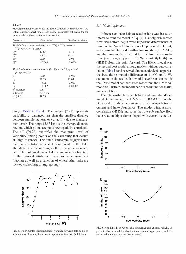
Table 2Model parameter estimates for the model structure with the lowest AICvalue (autocorrelated model) and model parameter estimates for thesame model without spatial autocorrelation

Parameter Mean value Standard deviation

Model without autocorrelation term: nacβ0+nacβ1current

2+nacβ2current+

nacβ3depthβ0nac 12.68 0.49β1nac −5.73 13.5β2nac 2.90 2.92β3nac −0.006 0.0004

Model with autocorrelation term β0+β1current2+β2current+

β3depth+S(x)β0 8.20 0.992β1 20.28 12.04β2 −3.75 3.009β3 −0.0025 0.00087τ2 (nugget) 2.81ϕ (range) 3.67 kmσ2 (sill) 39.28

243V.N. Agostini et al. / Journal of Marine Systems 71 (2008) 237–248

range (Table 2, Fig. 4). The nugget (2.81) representsvariability at distances less than the smallest distancebetween sample stations or variability due to measure-ment error. The range (2.67 km) is the average distancebeyond which points are no longer spatially correlated.The sill (39.28) quantifies the maximum level ofvariability among points or the variability that occursat large distances. The fitted variogram suggests thatthere is a substantial spatial component to the hakeabundance after accounting for the effects of current anddepth. In biological terms, hake abundance is a functionof the physical attributes present in the environment(habitat) as well as a function of where other hake arelocated (schooling or aggregating).

Fig. 4. Experimental variogram (semi-variance between data points asa function of distance) fitted to an exponential function (solid line).

3.1. Model inference

Inference on hake habitat relationships was based oninference from the model in Eq. (4). Namely, sub-surfaceflow and bottom depth were important determinants ofhake habitat. We refer to the model represented in Eq. (4)as the hake habitat model with autocorrelation (HHMAC),and the same model structural form without autocorrela-tion (i.e., y= β0 + β1current

2+β2current+β3depth) as(HMM) from this point forward. The HMM model wasthe second best model among models without autocorre-lation (Table 1) and received almost equivalent support asthe best fitting model (difference of 1 AIC unit). Wecomment on the results that would have been obtained ifthe HMMmodel had been used rather than the HMMACmodel to illustrate the importance of accounting for spatialautocorrelation.

The relationship between habitat and hake abundanceare different under the HMM and HMMAC models.Both models indicate curvi-linear relationships betweencurrent and hake abundance. The model without auto-correlation (HMM) indicates that the sub-surface flowhake relationship is dome-shaped with current velocities

Fig. 5. Relationship between hake abundance and current velocity aspredicted by the model without autocorrelation (upper panel) and themodel with autocorrelation (lower panel).

Fig. 6. Predicted hake habitat given bottom depth and undercurrent velocities. Light grey represents less suitable habitat (number of fishb1100), darkgrey represents more suitable habitat (number of fishN1100). Pie charts represent overall habitat distribution for 1995 and 1998.

244 V.N. Agostini et al. / Journal of Marine Systems 71 (2008) 237–248

near zero leading to higher amount of favorable hakehabitat (Fig. 5a). The best formulation for the model withautocorrelation (HMMAC) shows the opposite trend,with high and low flow velocities leading to higheramount of favorable hake habitat (Fig. 5b). The directionof the velocity did not appear to be important in theHMMAC model, however (Fig. 5b). In addition, theeffect of depth is diminished (smaller absolute value ofcoefficient) in the HMMAC model (Table 2). Tosummarize, high quality hake habitat would have beenexpected at low current velocities under the HMMmodel, whereas high quality hake habitat would beexpected at greater velocities in the HMMAC model.

Predicted hake habitat in 1995 was calculated byimplementing the mean effect component of Eq. (4)using model coefficients from the HMMAC model andcovariate values (depth and current velocity) fromsampling stations in 1995 (Fig. 6). In addition, pre-dictions of hake habitat under the physical conditions in1998 were also made (Fig. 6). The fit of the auto-correlation model to 1998 data is inferior to the fit to the1995 data (Fig. 7). More variability was explained byfitting a mean term to the observed 1998 data (residual

sums of squares of mean estimate=3549) than wasexplained by the 1995 model (residual sums of squaresestimate=5630). The pattern in Fig. 7 is similar toFig. 3a, suggesting that the spatial covariance structurewas different between 1998 and 1995. In particular, thespatial aggregations in 1998 may have been tighter, thusthe sill was probably higher and range shorter in 1998than 1995.

We defined hake habitat as favorable at locationwhere fish densities were higher than 1100 individualsand less favorable at locations where fish densities wereless than 1100 individuals, based on a break in thehistogram. Amount of favorable hake habitat was lowerin 1995 (16% of area considered in modeled) comparedto 1998 (51% of area considered in model) (Fig. 6).

4. Discussion

We use a Geostatistical approach to uncover potentialrelationships between hake and its environment. Thisapproach allows us to account for dependence betweendata points, a process we considered important in ouranalysis. Biologists have traditionally relied on methods

245V.N. Agostini et al. / Journal of Marine Systems 71 (2008) 237–248

developed for independent data, even though indepen-dence is an unrealistic assumption (Legendre, 1993).The simplifying assumption that datum from one pointin space is not influenced by another datum in the studyat another point in space rarely holds true (Carroll andPearson, 2000). The presence of an organism at aspecific site is induced by a number of major forces suchas ocean currents, winds and climate. It is also inducedby the presence of another organism at a neighboringsite. Conducting tests based on independence could leadto false identification of existing relationships.

Our results indicate that hake distribution is related topoleward flow (a dynamic variable) and bottom depth (astatic variable). This relationship was identified byincorporating a polynomial model (the mean effectcomponent) as well as a spatial autocorrelation com-ponent in our model. Including both of these compo-nents allowed us to identify and quantify importantrelationships. It is interesting to note that our resultsshow that the shape of the relationship between hakedistribution and poleward flow would have beendifferent if an autocorrelation component had not beenincluded. Identifying dynamic relationships such as theone between hake distribution and poleward flow ischallenging and tools effective at capturing dynamicrelationships as well as multiple processes are necessary.

Spatial approaches such as the one we used hereallow us to effectively explore mechanisms that mayexplain the distribution of fish populations. Such anunderstanding could not have been possible by simplyusing general linear models. An understanding of theprocess driving these distributions is essential in ourevaluation of the sustainability of fish stocks. Thus farfishery science has tended to evaluate managementperformance with indicators based on non-spatialpopulation dynamics models (Pauly et al., 2003),

Fig. 7. Fits of model with spatial autocorrelations predictions to 1998data. Units: log number of fish.

ignoring inherent spatial variability of a stock's distri-bution (Booth, 2000). For stocks such as Pacific hakewhere the biology of the fish has a spatial component,efforts should be made to incorporate spatial structure inindicators.

We have become increasingly aware of the distribu-tion patterns of many species, yet what drives thesedistributions is often poorly understood, makingprediction a difficult task (Verity et al., 2002). We toohad difficulty applying our model when attempting topredict habitat quantity in 1998; however, there wereseveral important differences between 1995 and 1998that may have affected predictions of abundance in1998. We applied the coefficients from the model fit to1995 data to predict habitat quality in 1998; however,our 1998 model fit (Fig. 7) clearly points out the needfor further refinement. Using a sub-set of the dataprobably introduced some measurement and processerror. The range of habitat considered in the model webuilt is located at the southern most edge of the adulthake distribution (38–43°N). This area is occupied by amixture of juveniles and adults. It is difficult todiscriminate acoustic signal of smaller sizes (juveniles)from signal for other organisms (e.g. euphasiids).Measurement error is introduced here, as smaller sizesmight not be fully reported. This could be one of theexplanations for the inferior fit of the model to the 1998data compared to the 1995 data, as in 1998 thepopulation reportedly shifted north (Wilson et al.,2000; Helser et al., 2002) and fewer adults wereobserved in southern areas. As can be seen in Fig. 7the model does not do well with predicting ‘0 values’(process error). Because of the shift north in thepopulation described above, the 1998 data set had ahigher number of locations with 0 fish. As a result, the1998 model predictions were not as accurate as the 1995model predictions. A model based on data from asection of the hake habitat located farther north (e.g.43°–48°N), where the majority of the populationsampled is older (fish size is bigger thus more accuratelysampled) and the area consistently occupied in both1995 and 1998, could have been more informative. Theinaccuracy of 1998 model predictions also suggests thatthe spatial autocorrelation function for the 1998 datamay be different than the autocorrelation function fit tothe 1995 data. These results also suggest that a uniquemodel should be fitted for El Niño years, as theHMMAC model was not robust to the two year types.

The three dimensional nature of the data setpresented another challenge. Our model representshake habitat in two dimensions (latitude and longitude);thus the three dimensional data had to be collapsed to

246 V.N. Agostini et al. / Journal of Marine Systems 71 (2008) 237–248

two dimensions. There are a number of ways the under-current could have been represented in the model; wechose an average of current values in the 130–220 mdepth bins and measured the flow relative to the pole-ward direction (i.e., current could have a negativevalue). This choice might have affected our results byfocusing on an aspect of the current that may not havebeen the most relevant to fish distribution. The reso-lution of the acoustic data set used in this study allowedus to examine hake habitat over a wide geographic rangeat fine detail. Although powerful, this also presentedsome challenges. The data set we used for this analysiswas very large (information on flow characteristics andhake spanning 15° of latitude, ∼300,000 grid points/year). Because of the large nature of the data set (thusthe computational power necessary to build a modelbased on data from the entire hake distribution range),we used a sub-set of the data in our analysis as outlinedabove in the methods section. This allowed us to testapproaches and methods that could in the future beapplied to the entire data set and additional years.

The main aim of this study was to develop aquantitative measure of hake habitat. Our goal was todevelop a metric that would quantify importantphysical–biological linkages in the California CurrentEcosystem. Given the relationship between hakedistribution and the physical structure of the CCdescribed by a number of authors (Smith et al., 1990;Dorn, 1995; Benson et al., 2002; Agostini et al., 2006)and the importance of hake in the CC food web (Field,2004) hake habitat was explored as a suitable metric.Our results indicate that climate forcing affects thespatial structure of hake habitat. Hake habitat in ourstudy area expands during a warm year El Niño year(1998) and contracts during a cold year (1995) (Fig. 6).Agostini et al. (2006) suggest that this may be due tochanges in the intensity and location of the polewardcurrent. Our study supports this hypothesis, and point tothe importance of accounting for physical processes inthe study of fish distribution.

In this study we apply a spatial approach to outlinehake habitat areas, and examine how climate forcingmay affect these areas. This addresses both spatial andenvironmental processes of the CC system, facilitatingthe inclusion of broader ecosystem considerations andobjectives in single species assessments and manage-ment plans. While detailed single species assessmentsstill form the core of management advice in most cases,they are increasingly embedded in an ecosystem con-text, at least qualitatively (Mace, 2001). However, anumber of important classes of ecosystem interactionsare currently not being routinely evaluated (Sissenwinse

and Murawski, 2004). Amongst these are relationshipsbetween biological and physical components of ecosys-tems. The stability of biological communities is affectedby the interaction between life history, environmentalvariation and fishing strategies (Sissenwinse andMurawski, 2004). Accounting for interactions betweenbiological and physical components of the ecosystemsuch as the one we examine here will not only help usevaluate important ecosystem interactions, but it willalso help determine appropriate spatial scales of datacollection, science and management presently missingfrom conventional single species management (Hilborn,2004).

The desire to represent key ecosystem interactionshas lead to the recent focus on ecosystem indices. Anumber of symposia and working groups have beenconvened on this topic (e.g.: “Ecosystem Considerationsin Fishery Management”, Anchorage 1998; “Respon-sible Fishing in the Marine Environment”, Reykjavik2001; IOC-SCOR working group 119, “QuantitativeIndicators for Fisheries Management”, Paris 2004;“Advancing Scientific Advice for an Ecosystem Ap-proach to Fisheries”, Dublin 2004). Most of the indicesdeveloped to date represent trophic interactions, whilework on indices representing interactions betweenspecies and the physical environment is lagging behind.Climate forcing of ecosystems has mostly beendescribed by large scale indices such as PDO andENSO. Climate impacts are aggregated across largespatial scales and range of species and direct links aremade between climate forcing and production varia-bility. However, changes in ecosystem structure areoften the result of changes in physical habitat with verydistinct spatial structure. In order to fully describeecosystems, spatially explicit indices directly represent-ing physical–biological linkages should also bedeveloped.

The focus of this study on pelagic habitat of a keytrophic species addresses this issue. A quantitativemeasure of hake habitat such as the one we develop herecould potentially serve as an ecosystem indicator. Hakeis one of the major predators in the northern CC system.The amount and distribution of adult hake habitat haslarge implications for the Pacific Northwest food web.For example Field (2004) found that during warm yearswhen hake are more abundant in northern CC waters(north of Cape Mendocino), there is an increase inpredation (particularly on pandalid shrimp and smallflatfish) and competition (for euphausiids, forage fishand other prey of resident groundfish). The absence orpresence of hake in Pacific Northwest waters is likelyrelated to habitat suitability along its range of

247V.N. Agostini et al. / Journal of Marine Systems 71 (2008) 237–248

distribution. Changes in the amount of adult hakehabitat could serve as an indicator of changes in thestructure/energy flow of the northern CC ecosystem, aschanges in hake distribution could imply changes in theproductivity of other commercially and ecologicallyimportant species. Metrics able to detect these types ofchanges could be good ecosystem indicators, as they arerelated to both the physical and biological structure ofthe ecosystem. Examples of potential ecosystemindicators are: % of hake habitat distributed north ofLatitude X, % of hake habitat distributed offshore oflongitude X, % of overall habitat defined as suitablehake habitat, favorable/unfavorable habitat, (favorablehabitat)t+1− (favorable habitat)t.

Spatial structure and environmental processes arediscussed as essential to the development EcosystemBased Fishery Management (EBFM). However, as wedevelop approaches to implement EBFM, habitat issues arenot receiving the attention they warrant. Most of the workon habitat focuses on benthos, with knowledge of pelagichabitat lagging behind. Studies such as this one will help toincrease the awareness of pelagic habitat and contribute tothe development of effective EBFM strategies.

Acknowledgments

We thankMike Guttormsen for help with acoustic dataprocessing; Elizabeth Babcock, Jodie Little, and WarrenWooster for helpful discussion and review of thismanuscript; John Mickett for help with programmingand Amity Femia for help with graphics. This study wassupported by the JISAO/Climate Impacts Group (Uni-versity of Washington) under NOAA CooperativeAgreement NAI17RJ123, contribution # XXX. S.D.Pierce was partially supported by National Oceanic andAtmospheric Administration (Grant AB133F05SE4205).

References

Agostini, V.N., Francis, R.C., Hollowed, A.B., Pierce, S., Wilson, C.,Hendrix, A.N., 2006. The relationship between hake (Merlucciusproductus) distribution and poleward sub-surface flow in theCalifornia current system. Canadian Journal of Fishery andAquatic Sciences 63, 2648–2659.

Barange, M., Hampton, I., 1997. Spatial structure of co-occurringanchovy and sardine populations from acoustic data: implicationsfor survey design. Fisheries Oceanography 6, 94–108.

Barange, M., Coetzee, J.C., Twatwa, N.M., 2005. Strategies of spaceoccupation by anchovy and sardine in the southern Bengulea: therole of stock size and intra-species competition. ICEAS Journal ofMarine Science 62, 645–654.

Beamish, R.J., McFarlane, G.A., King, J.R., 2000. Fisheriesclimatology: understanding decadal scale processes that naturallyregulate British Columbia fish populations. In: Harrison, P.J.,

Parsons, T.R. (Eds.), Fisheries Oceanography: An IntegrativeApproach to Fisheries Ecology and Management. BlackwellScience, Oxford, pp. 94–145.

Benson, A.J., McFarlane, G.A., Allen, S.E., Dower, J.F., 2002.Changes in Pacific hake (Merluccius productus) migration patternsand juvenile growth related to the 1989 regime shift. CanadianJournal of Fishery and Aquatic Sciences 59, 1969–1979.

Booth, A.J., 2000. Incorporating the spatial component of fisheriesdata into stock assessment models. ICES Journal of MarineScience 57, 858–865.

Burnham, K.P., Anderson, D.R., 2002. Model Selection and Multi-model Inference: A Practical Information—Theoretic Approach,2nd Edition. Springer-Verlag, New York, New York, USA.

Carroll, S., Pearson, D., 2000. Detecting and modeling spatial andtemporal dependence in conservation biology. ConservationBiology 14 (6), 1893–1897.

Chambers, J.M., Hasties, T.J., 1992. StatisticalModels in S.Wadsowrthand Brooks Cole Advanced Books, Pacific Grove, California.

Conan, G.Y., Maynou, F., Stloyarenko, D., Mayer, L., 1994. Mappingand assessment of fisheries resources with coastal and depthconstraints, the case study of snow crab in the Bay of Islands Fjord(Newfoundland). ICES C.M. 1994/B+D+G+H: 4. InternationalCouncil for the Exploration of the Sea, Charlottenlund, Denmark.

Cressie, N.A.C., 1993. Statistics for Spatial Data. John Wiley andSons, Inc., New York, New York, USA.

Diggle, P.J., Tawn, J.A., Moyeed, R.A., 1998. Model-based geosta-tistics. Applied Statistics 47 (3), 299–350.

Dorn, M.W., 1995. The effects of age composition and oceanographicconditions on the annual migration of Pacific Whiting,Merlucciusproductus. CalCOFI Reports 36, 97–105.

Erofeeva, S.Y., Egbert, G.D., Kosro, P.M., 2003. Tidal currents on thecentral Oregon shelf: models, data, and assimilation. Journal ofGeophysical Research 108, 3148.

Field, J.C., 2004. Application of ecosystem-based fishery managementapproaches in the Northern California Current. PhD Dissertation.University of Washington.

Fletcher, W.J., Summer, N.R., 1999. Spatial distribution of sardine(Sardinops sagax) eggs and larvae: an application of geostatisticsand resampling survey data. Canadian Journal of Fisheries andAquatic Sciences 56, 907–914.

Francis, R.C., Adlerstein, S.A., Hollowed, A.B., 1989. Importance ofenvironmental fluctuations in the management of Pacific hake. In:Beamish, R.J., McFarlane, G.A. (Eds.), Effects of OceanVariability on Recruitment and an Evaluation of ParametersUsed in Stock Assessment Models. Special Publication of theCanadian Journal of Fisheries and Aquatic Sciences, 108.

Hare, S.R., Mantua, N.J., 2000. Empirical evidence for North Pacificregime shifts in 1977 and in 1989. Progress in Oceanography 47(103), 145.

Helser, T.E., Methot, R.E., and Fleischer, G.W., 2002. Stock assessmentof Pacific hake in U.S. and Canadian Waters in 2003. NorthwestFisheries Science Center, National Marine Fisheries Service.

Helser, T.E., Methot, R.E. and Fleischer, G.W., 2004. Stock assessmentof Pacific hake in U.S. and Canadian Waters in 2003. NorthwestFisheries Science Center, National Marine Fisheries Service.

Hilborn, R., 2004. Ecosystem-based fisheries management: the carrotor the stick? Marine Ecology, Progress Series 274, 269–303.

Horne, J.K., Schneider, D.C., 1995. Spatial variance in ecology. Oikos74, 1–9.

Kracker, L., 1999. The geography of fish: the use of remote sensingand spatial analysis tools in fisheries research. ProfessionalGeographer 51 (3), 440–450.

248 V.N. Agostini et al. / Journal of Marine Systems 71 (2008) 237–248

Legendre, P., 1993. Spatial autocorrelation: trouble or new paradigm?Ecology 74, 1659–1673.

Livingston, P.A., Bailey, K.M., 1985. Trophic role of the Pacificwhiting, Merluccius productus. Marine Fisheries Review 47 (2),16–22.

MacCall, A.D., 1996. Patterns of low-frequency variability in fishpopulations of the California current. CalCOFI Report 37,100–110.

Mace, P.M., 2001. A new role for MSY in single-species andecosystem approaches to fisheries stock assessment and manage-ment. Fish and Fisheries 2, 2–32.

Maravelias, C.D., Reid, D.G., Simmonds, E.J., Haralabous, J., 1996.Spatial analysis and mapping of acoustic survey data in thepresence of high local variability: geostatistical application toNorth Sea herring (Clupea harengus). Canadian Journal ofFisheries and Aquatic Sciences 53, 1497–1505.

McFarlane, G.A., Beamish, R.J., 1985. Biology and fishery of PacificWhiting, Merluccius productus, in the Strait of Georgia. MarineEcology, Progress Series 47, 23–34.

McNaughton, S.J., Wolf, L.L., 1973. General Ecology. Holt, Rinehartand Winston, New York, New York, USA.

Pauly, D., Watson, R., Christensen, V., 2003. Ecological geography asa framework for transition toward responsible fishing. In: Sinclair,M., Valdimarsson, G. (Eds.), Responsible Fisheries in the MarineEcosystem. FAO, Rome, pp. 87–101.

Pedersen, M., 1985. Puget Sound Pacific Whiting, Merlucciusproductus, resource and industry: an overview. Marine FisheriesReview 47, 35–38.

Petitgas, P., 1993. Geostatistics for stock assessment: a review and anacoustic application. ICES Journal of Marine Sciences 50, 285–298.

Petitgas, P., 1998. Biomass-dependent dynamics of fish spatialdistributions characterized by geostatistical aggregation curves.ICES Journal of Marine Sciences 55, 443–453.

Petitgas, P., 2001. Geostatistics in fishery survey design and stockassessment: models, variances and applications. Fish and Fisheries2, 231–249.

Petitgas, P., Poulard, J.C., 1989. Applying stationary geostatistics tofisheries: a study on hake in the Bay of Biscay. ICES C.M./G:62.International Council for the Exploration of the Sea, Charlotten-lund, Denmark.

Pierce, S.D., Smith, R.L., Kosro, P.M., Barth, J.A., Wilson, C.D.,2000. Continuity of the poleward undercurrent along the easternboundary of the mid-latitude north Pacific. Deep Sea Research. (II)47, 811–829.

Ribiero,Diggle, P.J., 2001.Apackage for geostatistical analysis. R-NEWS1 (2), 15–18 ISSN 1609–3631, WWW Page, http://cran.R-project.org/doc/Rnews.

Rice, J., 2001. Implications of variability on many time scales forscientific advice on sustainable management of living marineresources. Progress in Oceanography 49, 189–209.

Rossi, R.E., Mulla, D.J., Journel, A.G., Franz, E.H., 1992.Geostatistical tools for modeling and interpreting ecologicalspatial dependence. Ecological Monographs 62 (2), 277–314.

Simard, Y., Legendre, P., Lavoie, G., Marcotte, D., 1992. Mapping,estimating biomass, and optimizing sampling programs forsptailly autocorrelated data: case study of the northern shrimp(Pandalus borealis). Canadian Journal of Fisheries and AquaticSciences 49, 32–45.

Sissenwinse, M.P., Murawski, S., 2004. Moving beyond intelligenttinkering: advancing an ecosystem approach to fisheries. MarineEcology, Progress Series 274, 291–295.

Smith, B.D., McFarlane, G.A., Saunders, M.W., 1990. Variations inPacific hake (Merluccius productus) summer lenght-at-age nearsouthern Vancouver Island and its relationship to fishing andoceanography. Canadian Journal of Fisheries and Aquatic Sciences47, 2195–2211.

Verity, P.G., Smetacek, V., Smayda, R.J., 2002. Status, trends and thefuture of marine pelagic ecosystem. Environmental Conservation29, 207–237.

Ware, D.M., McFarlane, G.A., 1995. Climate-induced changes inPacific hake abundance and pelagic community interactions in theVancouver island upwelling system. In: Beamish, R.J. (Ed.),Climate Change and Northern Fish Populations. Special Publica-tion of the Canadian Journal of Fisheries and Aquatic Sciences,121, pp. 509–521.

Wiebe, P.H., Beardsley, R.C., Mountain, D.G., Bucklin, A., 1996.Global ocean ecosystem dynamics: initial program in NorthwestAtlantic. Sea Technology 37 (8), 67–76.

Wilson, C.D., Guttormsen, M.A., 1997. Echo integration trawl surveyof Pacific hake, Merluccius productus, off the Pacific coast of theUnited States and Canada during July–August 1998. NOAATech.Memo. NMFS AFSC-74, Seattle Wash.

Wilson, C.D., Guttorsmen, M.A., Cooke, K., Saunders, M.W., Kieser,R., 2000. Echo integration-trawl survey of Pacific hake,Merluciusproductus, off the Pacific Coast of the United States and Canadaduring July–August, 1998. NOAA Technical Memorandum.NMFS-AFSC-118.