Clustering and Dimensionality Reduction

Brendan and Yifang April 21 2015

Pre-knowledge• We define a set A, and we find the element that

minimizes the error

• We can think of as a sample of

• Where is the point in C closest to X.

Clustering methods

• K-means clustering• Hierarchical clustering• Agglomerative clustering• Divisive clustering• Level set clustering•Modal clustering

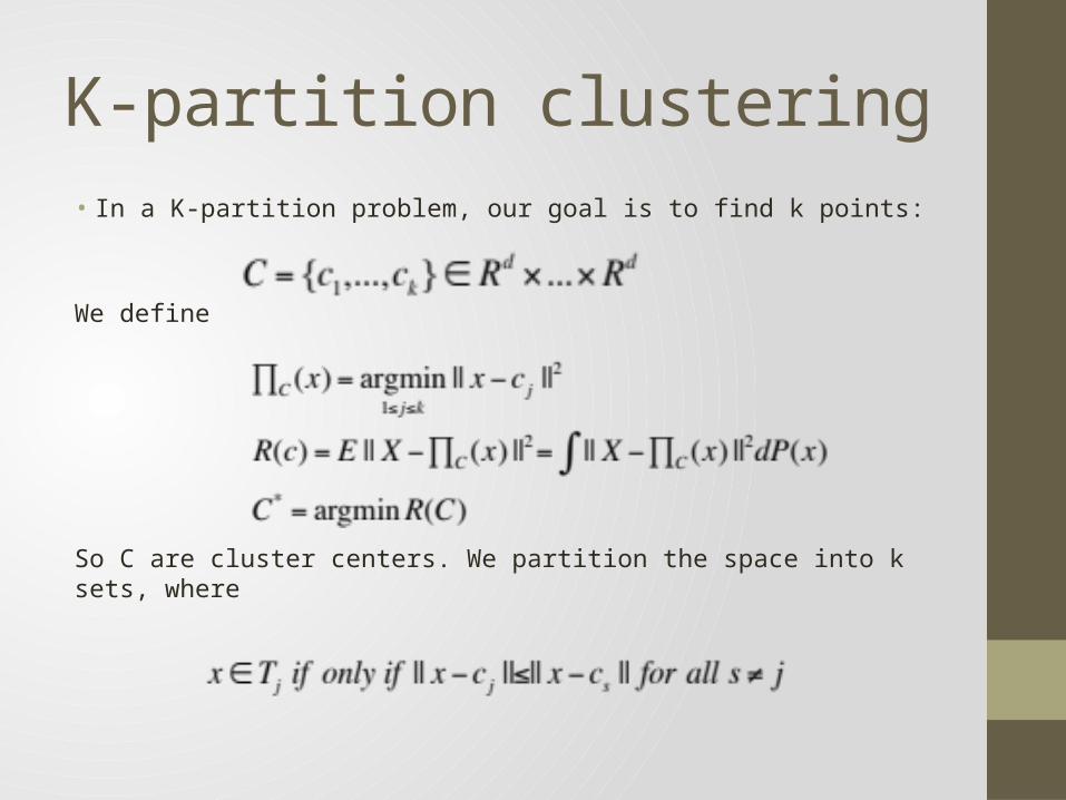
K-partition clustering • In a K-partition problem, our goal is to find k points:

We define

So C are cluster centers. We partition the space into k sets, where

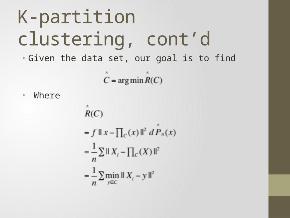
K-partition clustering, cont’d• Given the data set, our goal is to find

• Where

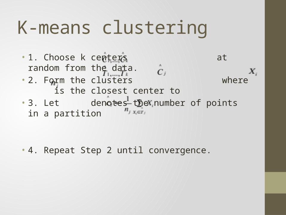
K-means clustering• 1. Choose k centers at random from the data.• 2. Form the clusters where is the closest center to • 3. Let denotes the number of points in a partition

• 4. Repeat Step 2 until convergence.

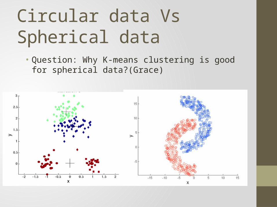
Circular data Vs Spherical data

• Question: Why K-means clustering is good for spherical data?(Grace)

• Question: What is relationship between K-means and Naïve Bayes?

• Answer: They have the followings in common: • 1. Both of them estimate a probability density function.• 2. Assign the closest category/label to the target point (Naïve

Bayes), assign the closest centroid to the target point (K-means)• They are different in these aspects:• 1. Naïve bayes is supervised algorithm, K-means is an

unsupervised method.• 2. K-means is optimization task, and it is an iterative process, but

Naïve bayes is not. • 3. K-means is like to a multiple runs of Naïve Bayes, and in each

run, the labels are adaptively adjusted.

• Question: Why K-means does not work well for Figure 35.6? Why spectral clustering helps with it? (Grace)

• Answer: Special clustering maps data points in Rd to data points in Rk. Circle-shaped data points in Rd will be spherical-shape in Rk. But special clustering involves matrix decomposition, is rather time-consuming.

Agglomerative clustering• Requires pairwise distance among clusters. • There are three commonly employed distance.• Single linkage• Complete linkage (Max Linkage)• Average linkage

1. Start with each point in a separate cluster2. Merge the two closest clusters.3. Go back to step 1

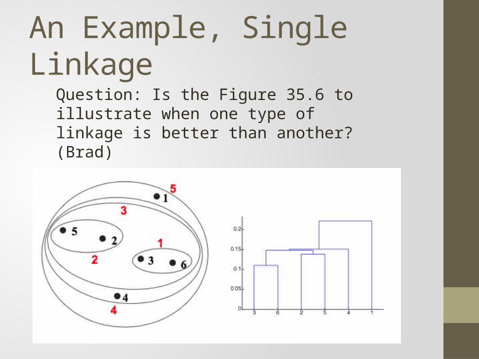
An Example, Single LinkageQuestion: Is the Figure 35.6 to illustrate when one type of linkage is better than another? (Brad)

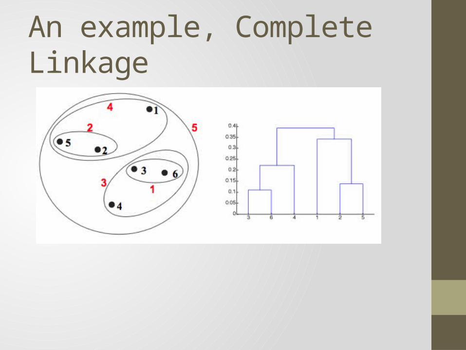
An example, Complete Linkage

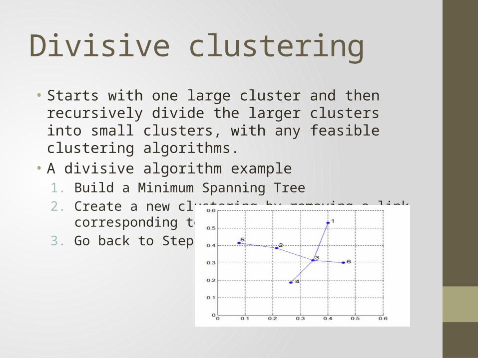
Divisive clustering• Starts with one large cluster and then recursively divide the

larger clusters into small clusters, with any feasible clustering algorithms.

• A divisive algorithm example1. Build a Minimum Spanning Tree 2. Create a new clustering by removing a link corresponding to

the largest distance3. Go back to Step 2

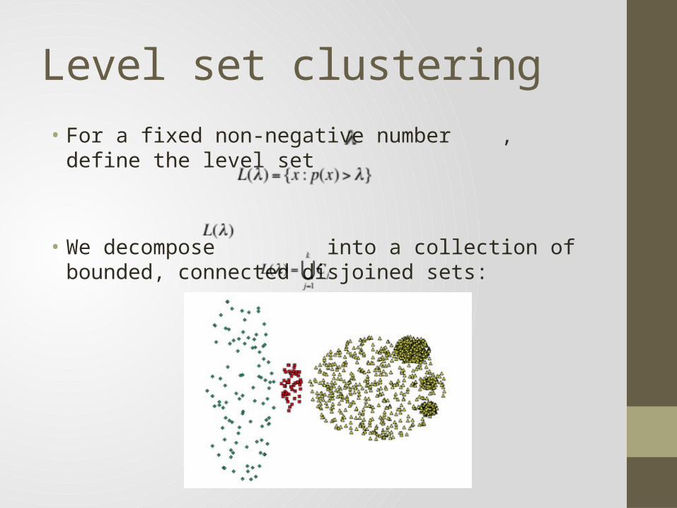
Level set clustering• For a fixed non-negative number , define the level set

• We decompose into a collection of bounded, connected disjoined sets:

Level Set Clustering, Cont’d• Estimate density distribution function: Using KDE

• Decide : fix a small number

• Decide :•

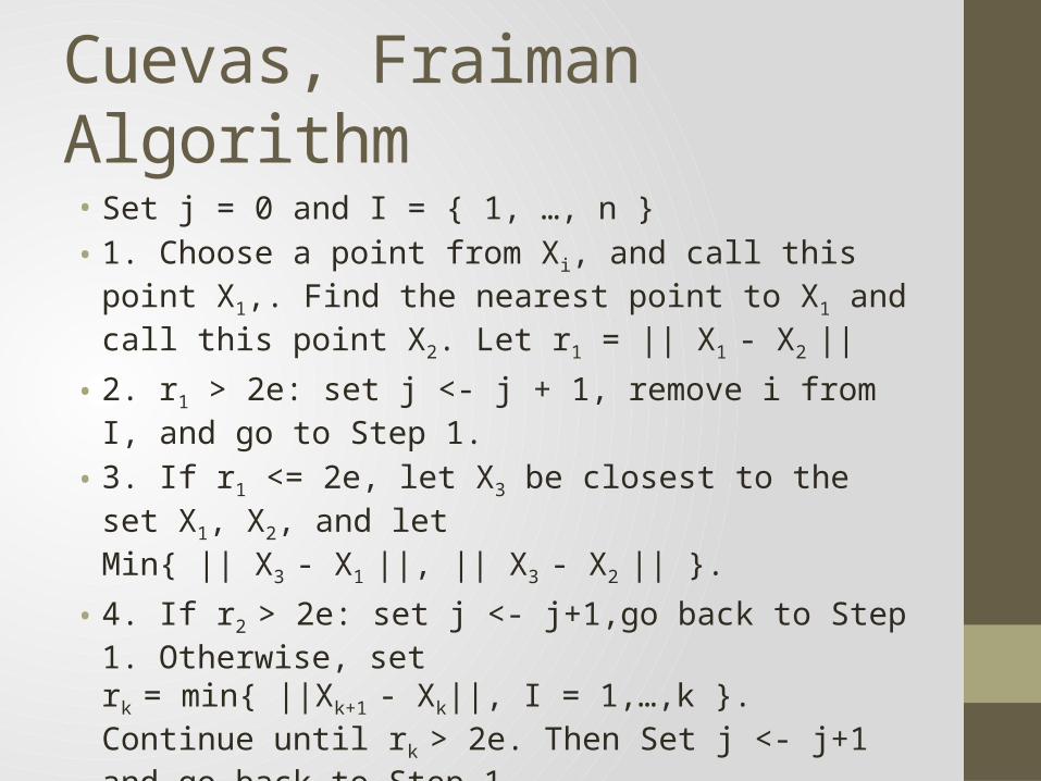
Cuevas, Fraiman Algorithm• Set j = 0 and I = { 1, …, n }• 1. Choose a point from Xi, and call this point X1,. Find the

nearest point to X1 and call this point X2. Let r1 = || X1 - X2 ||

• 2. r1 > 2e: set j <- j + 1, remove i from I, and go to Step 1.

• 3. If r1 <= 2e, let X3 be closest to the set X1, X2, and let Min{ || X3 - X1 ||, || X3 - X2 || }.

• 4. If r2 > 2e: set j <- j+1,go back to Step 1. Otherwise, set rk = min{ ||Xk+1 - Xk||, I = 1,…,k }. Continue until rk > 2e. Then Set j <- j+1 and go back to Step 1.

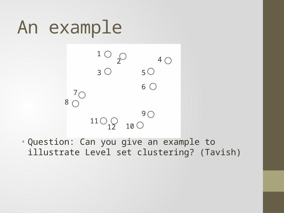
An example

• Question: Can you give an example to illustrate Level set clustering? (Tavish)

21

5

4

3

78

12

9

10

6

11

Modal Clustering

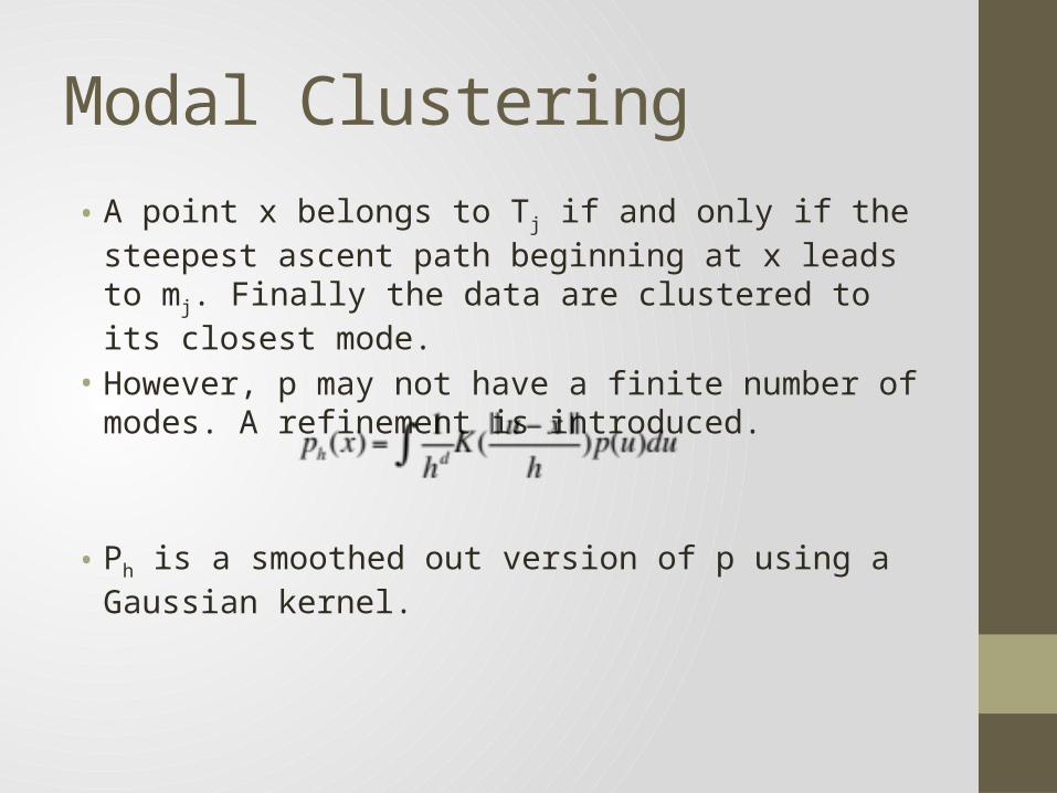
• A point x belongs to Tj if and only if the steepest ascent path beginning at x leads to mj. Finally the data are clustered to its closest mode.

• However, p may not have a finite number of modes. A refinement is introduced.

• Ph is a smoothed out version of p using a Gaussian kernel.

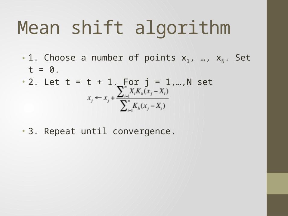
Mean shift algorithm

• 1. Choose a number of points x1, …, xN. Set t = 0.• 2. Let t = t + 1. For j = 1,…,N set

• 3. Repeat until convergence.

• Question: Can you point out the differences and similarities between different clustering algorithms?(Tavish)

• Can you compare the pros and cons of the clustering algorithms, and what are suitable situations for each of them?(Sicong)

• What is the relationship between the clustering algorithms? What assumptions do they have?(Yuankai)

• Answer: • K-means• Pros: • 1. Simple, very intuitive. Applicable to almost any scenario, any

dataset. • 2. Fast algorithm

• Cons: • 1. does not work for density-varying data

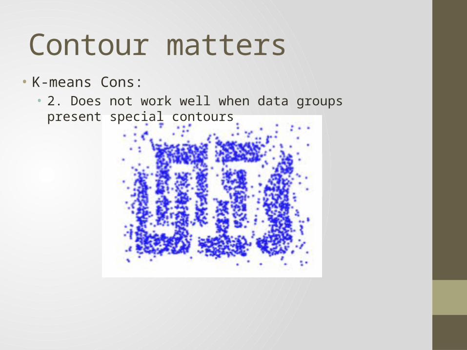
Contour matters• K-means Cons: • 2. Does not work well when data groups present special contours

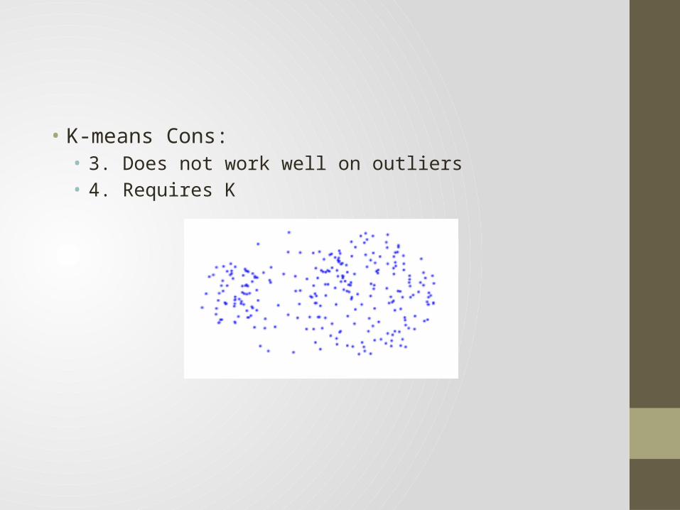
• K-means Cons: • 3. Does not work well on outliers• 4. Requires K

• Hierarchical clustering• Pros: • 1. Its clustering result has the clusters at any level granularity. Any

number of clusters could be achieved by cutting the dendrogram at a corresponding level.

• 2. It provides a dendrogram, which could be visualized hierarchical tree.

• 3. Does not requires a specified K.• Cons:• 1. Slower than K-means• 2. Hard to decide where to cut off the dendrogram

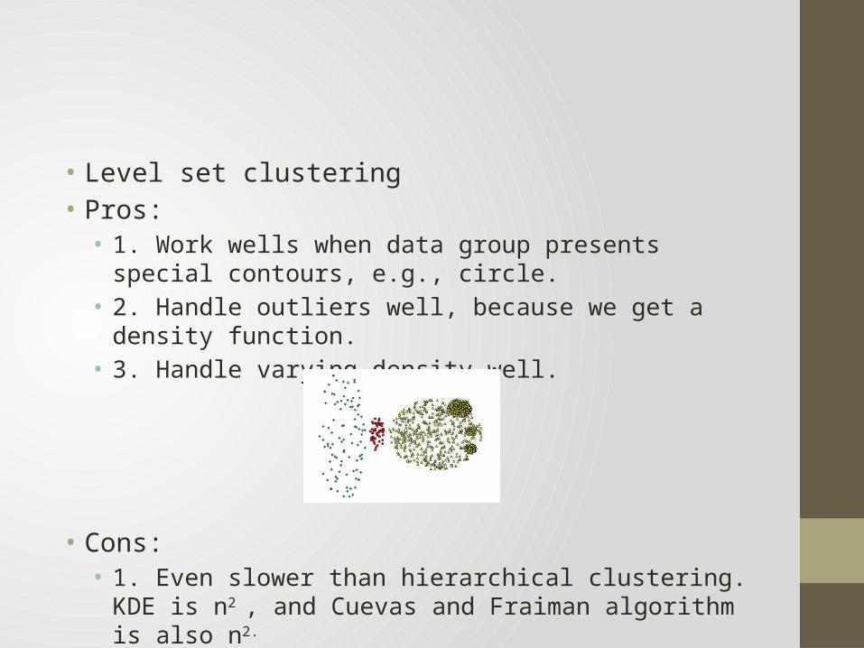
• Level set clustering• Pros: • 1. Work wells when data group presents special contours, e.g.,

circle.• 2. Handle outliers well, because we get a density function.• 3. Handle varying density well.

• Cons:• 1. Even slower than hierarchical clustering. KDE is n2 , and Cuevas

and Fraiman algorithm is also n2.

• Question: Does K-means clustering guarantee convergence? (Jiyun)

• Answer: Yes. Its time complexity upper bound is O(n4)

• Question: In Cuevas-fraiman algorithm, does the choice of the start vertex matter? (Jiyun)

• Answer: The choice of start vertex does no matter.

• Question: Does not the choice of Xj in Mean shit algorithm matter?

• Answer: No. The Xj converges to the modes in the iterative process. The initial value does not matter.

Dimension Reduction

Motivation• Recall: Our overall goal is to find low-dimensional structure• Want to find a representation expressible with dimensions• Should minimize some quantization of the associated projection

error, ie

• In clustering, we found sets of points such that similar points are grouped together

• In dimension reduction, we focus more on the space (ie can we transform the space such that a projection preserves data properties while shedding excess dimensionality)

Question – Dimension Reduction BenefitsDimensionality reduction aims at reducing the number of random variables in the data before processing. However, this seems counterintuitive as it can reduce distinct features in the data set leading to poor results in succeeding steps. So, how does it help? - Tavish• Implicit assumption is that our data contains more features

than are useful/necessary (ie highly correlated or purely noise)• Common in big data• Common when data is naively recorded

• Reducing the number of dimensions produces a more compact representation and helps with the curse of dimensionality

• Some methods (ie manifold-based) avoid loss

Principal Component Analysis (PCA)• Simple dimension reduction technique• Intuition: project the data onto a -dimensional linear subspace

Question – Linear SubspaceIn Principal Component Analysis, it projects the data onto linear subspaces. Could you explain a bit about what is a linear subspace? - Yuankai• A linear subspace is a vector space subset of a higher

dimensional vector subspace

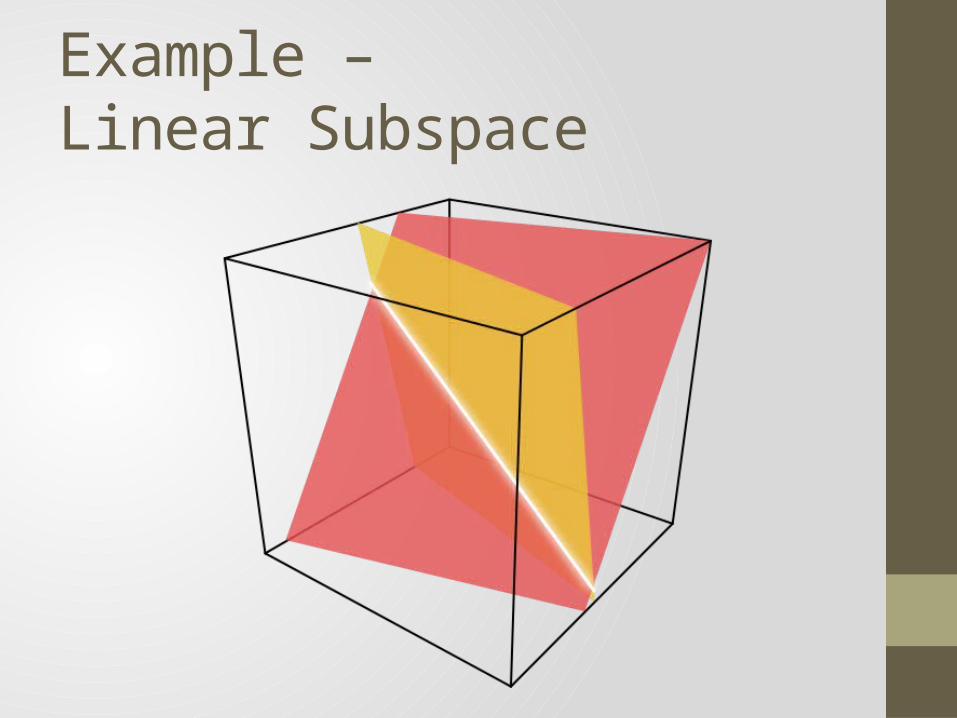
Example – Linear Subspace

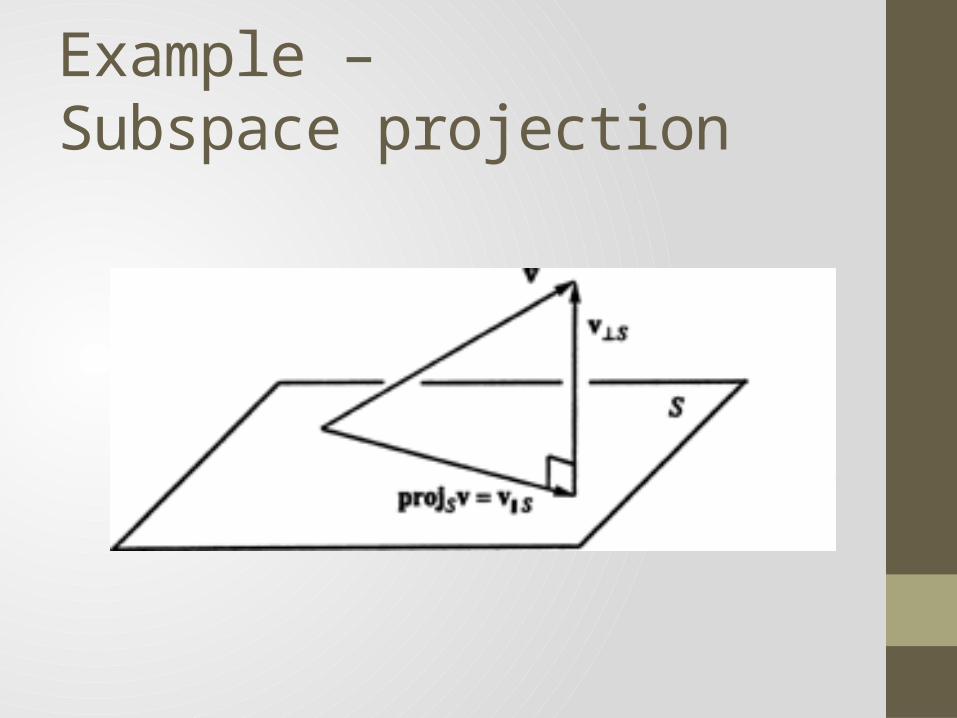
Example – Subspace projection

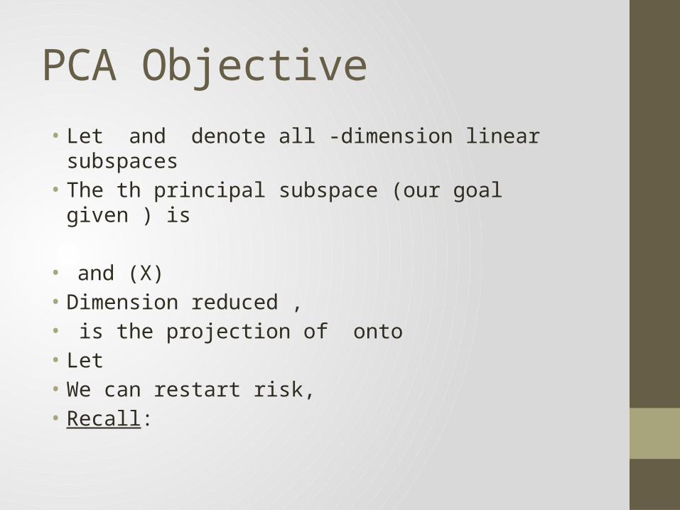
PCA Objective• Let and denote all -dimension linear subspaces• The th principal subspace (our goal given ) is

• and (X)• Dimension reduced , • is the projection of onto • Let • We can restart risk, • Recall:

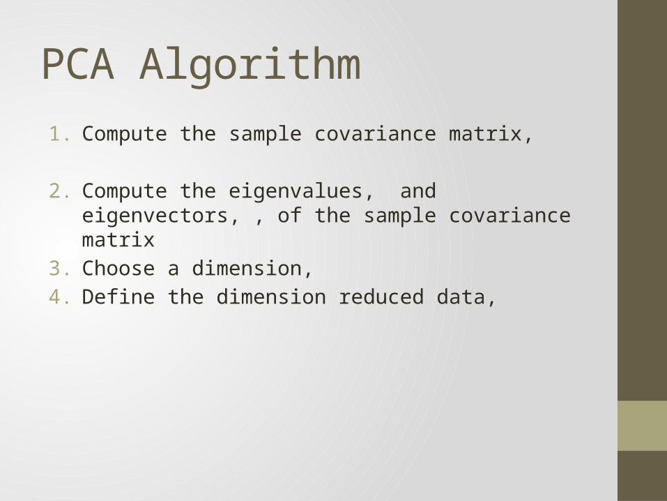
PCA Algorithm

1. Compute the sample covariance matrix,

2. Compute the eigenvalues, and eigenvectors, , of the sample covariance matrix

3. Choose a dimension, 4. Define the dimension reduced data,

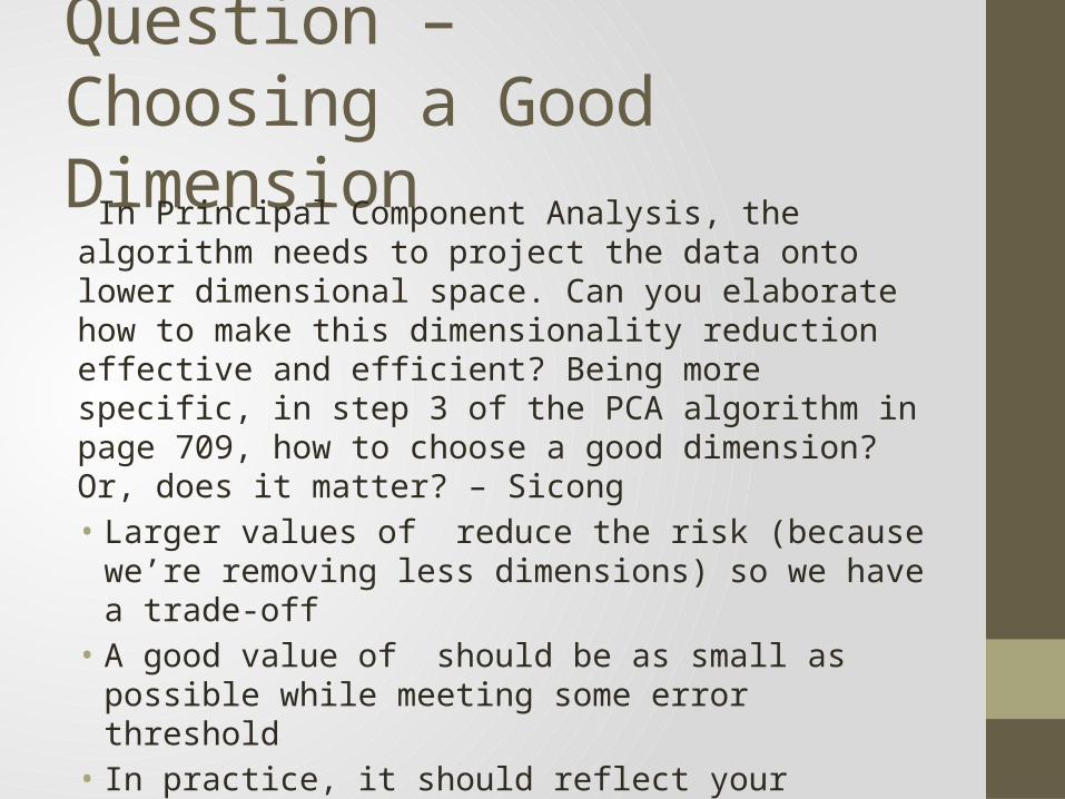
Question – Choosing a Good Dimension In Principal Component Analysis, the algorithm needs to project the data onto lower dimensional space. Can you elaborate how to make this dimensionality reduction effective and efficient? Being more specific, in step 3 of the PCA algorithm in page 709, how to choose a good dimension? Or, does it matter? – Sicong• Larger values of reduce the risk (because we’re removing less

dimensions) so we have a trade-off• A good value of should be as small as possible while meeting

some error threshold• In practice, it should reflect your computational limitations

PCA – Choosing • Book recommends fixing some and choosing

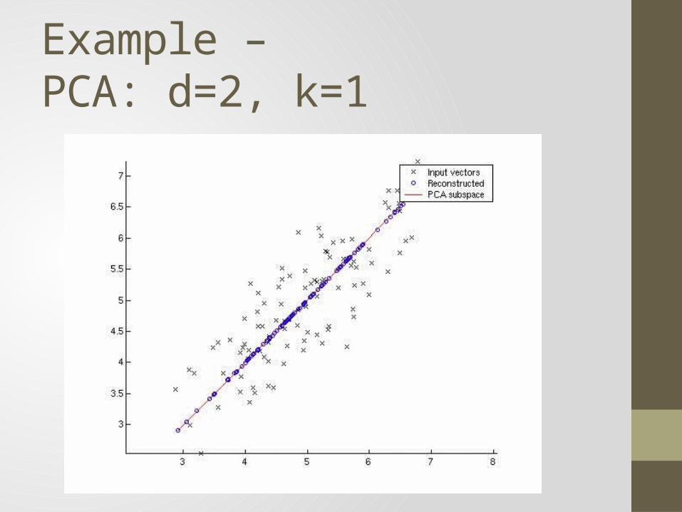
Example – PCA: d=2, k=1

Multidimensional Scaling• Instead of mean distance, we can instead try to preserve

pairwise distance• Given a mapping of points, ,• We can define a pairwise distance loss function• Let,

• This gives us an alternative to risk• We call the objective of finding the map to minimize ,

“Multidimensional scaling”• Insight: You can find by constructing a span out of the first

principal components

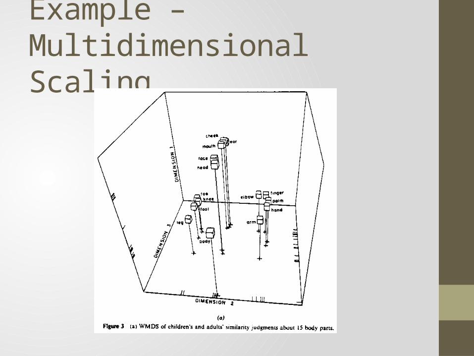
Example –Multidimensional Scaling

Kernel PCA• Suppose our data representation is less naïve, i.e. we’re given

a “feature map”,

• We’d still like to be able to perform PCA in the new feature space using pairwise distance

• Recall the covariance matrix in PCA was,

• In the feature space this becomes,

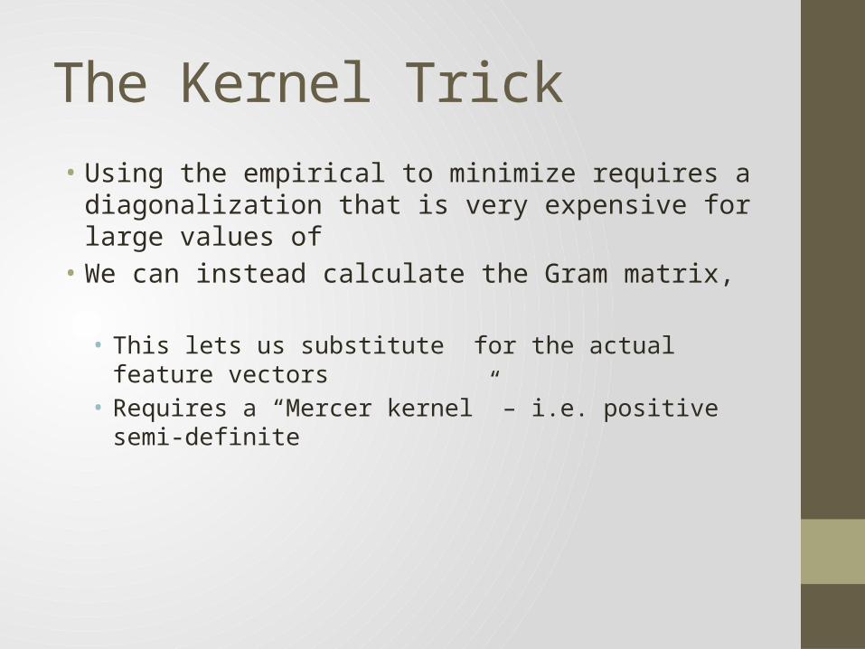
The Kernel Trick• Using the empirical to minimize requires a diagonalization that

is very expensive for large values of • We can instead calculate the Gram matrix,

• This lets us substitute for the actual feature vectors• Requires a “Mercer kernel” – i.e. positive semi-definite

Kernel PCA Algorithm

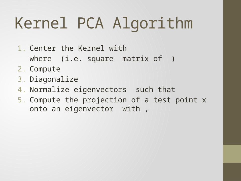
1. Center the Kernel with where (i.e. square matrix of )

2. Compute 3. Diagonalize 4. Normalize eigenvectors such that 5. Compute the projection of a test point x onto an eigenvector

with ,

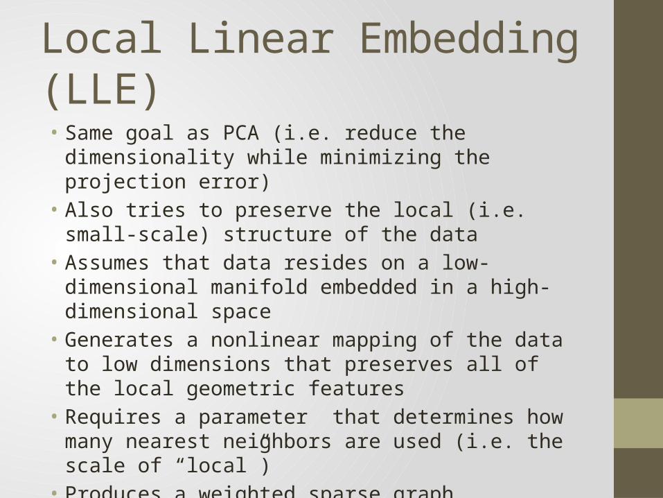
Local Linear Embedding (LLE)• Same goal as PCA (i.e. reduce the dimensionality while

minimizing the projection error)• Also tries to preserve the local (i.e. small-scale) structure of

the data• Assumes that data resides on a low-dimensional manifold

embedded in a high-dimensional space• Generates a nonlinear mapping of the data to low dimensions

that preserves all of the local geometric features• Requires a parameter that determines how many nearest

neighbors are used (i.e. the scale of “local”)• Produces a weighted sparse graph representation of the data

Question - Manifolds

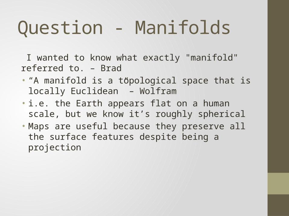
I wanted to know what exactly "manifold" referred to. – Brad• “A manifold is a topological space that is locally Euclidean” –

Wolfram• i.e. the Earth appears flat on a human scale, but we know it’s

roughly spherical• Maps are useful because they preserve all the surface features

despite being a projection

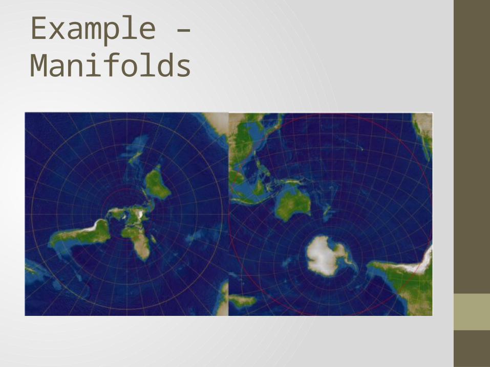
Example – Manifolds

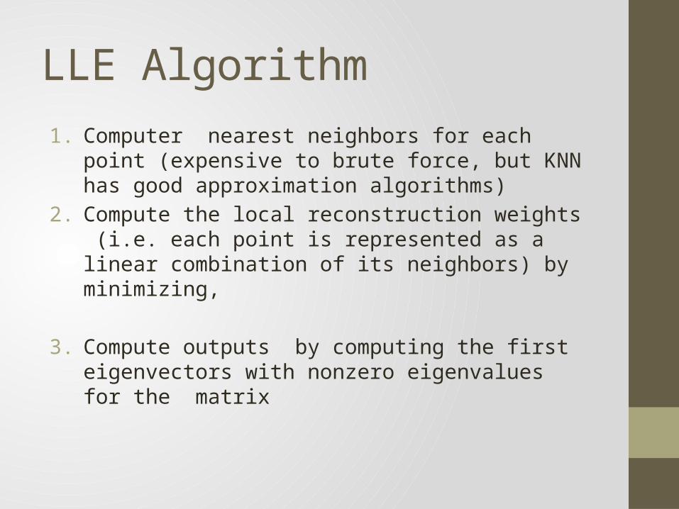
LLE Algorithm

1. Computer nearest neighbors for each point (expensive to brute force, but KNN has good approximation algorithms)

2. Compute the local reconstruction weights (i.e. each point is represented as a linear combination of its neighbors) by minimizing,

3. Compute outputs by computing the first eigenvectors with nonzero eigenvalues for the matrix

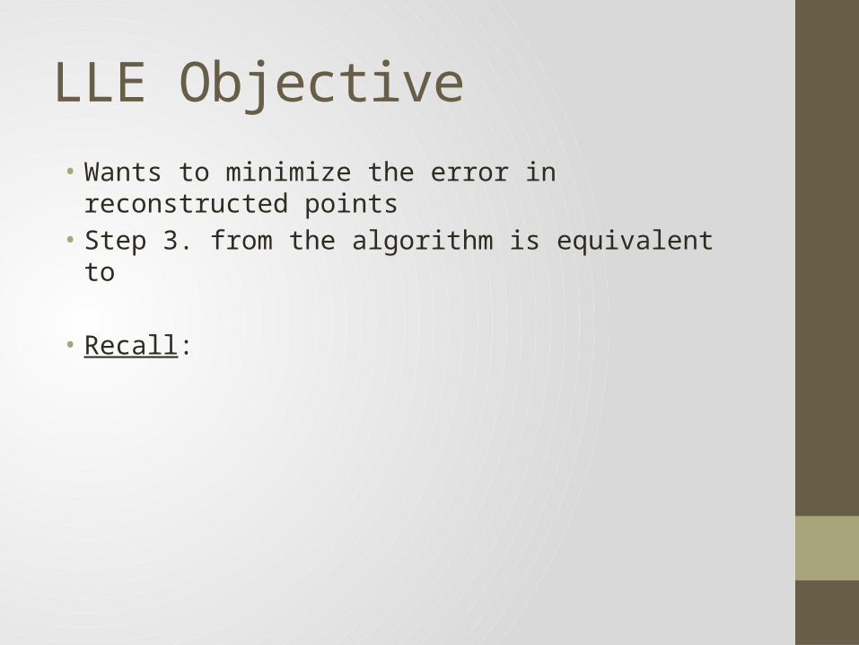
LLE Objective• Wants to minimize the error in reconstructed points• Step 3. from the algorithm is equivalent to

• Recall:

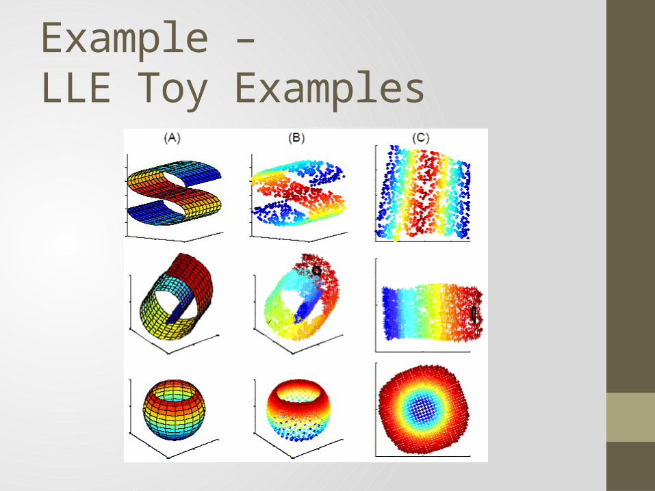
Example – LLE Toy Examples

Isomap• Similar to LLE in its preservation of the original structure • Provides a “manifold” representation of the higher

dimensional data• Assesses object similarity differently (distance, as a metric, is

computed using graph path length)• Constructs the low-dimensional mapping differently (uses

metric multi-dimensional scaling)

Isomap Algorithm

1. Compute KNN for each point and record a nearest neighbor graph, with vertices

2. Compute the graph distances using Dijkstra’s algorithms3. Embed the points into low dimensions using metric

multidimensional scaling

Laplacian Eigenmaps• Another similar manifold method• Analogous to Kernel PCA ?• Given kernel generated weights, , the graph Laplacian is given

by,

Where and • Calculate the first eigenvectors of , • They give an embedding,

• Intuition: eigenvector minimizes the weighted graph norm

Estimating the Manifold Dimension• Recall: These manifold methods all assume an embedded low-

dimensional manifold• We haven’t addressed how to find it if it isn’t given• It can be estimated from the provided data

• Consider a small ball, around some point on the manifold• Assume density is approximately constant on • The number of data points that fall in the ball is,

• Let be the smallest d-dimensional Euclidean ball around x containing j points

Estimating the Manifold Dimension Cont. • Given a sample • An estimate of the dimension is given by,

• Using KNN instead,

Principal Curves and Manifolds • We can, more generally, replace our linear subspaces with

non-linear ones• This non-parametric generalization of the principal

components is called “principal manifolds”• More formally, if we let be a set of functions from to , the

principal manifold is the functionthat minimizes,

Principal Curves and Manifolds Cont.• For computability, should be governed by some kernel (i.e.

quadratic functions, Gaussian, ect.)• should be expressible in the form,

• i.e. for Gaussian,

• Define a latent set of variables, where,

• Then the minimizer is given by

Random Projection• Making a random projection is often good enough• Key insight: when points in d dimensions are projected

randomly down onto dimensions, pairwise point distance is well preserved

• More formally let, , for some

• Then for a random projection ,

Question – Making a Random ProjectionSection 35.10 points out that the power of random projection is very surprising (for instance, the Johnson-Lindenstrauss Lemma). Can you talk more in detail about how to make random projection in class? – Sicong• Algorithm itself is very simple

1. Pick a -dimensional subspace at random2. Project all points onto the subspace normally 3. Calculate the maximum divergence in pairwise distances4. Repeat until maximum divergence is acceptable

• Computing the maximum divergence takes • Must be repeated ~ times in expectation• Takes in total

Question – Distance RandomizationWhy it important that the factor by which the distance between pairs of points changes during a random projection is limited? I can see how it's a good thing, but what is the significance of the randomness? – Brad• Randomness makes the projection trivial (algorithmically and

computationally - ) to compute• For some applications, preserving pairwise distance is

sufficient, i.e. multidimensional scaling