Embed Size (px)
Citation preview
10/3/2011
1
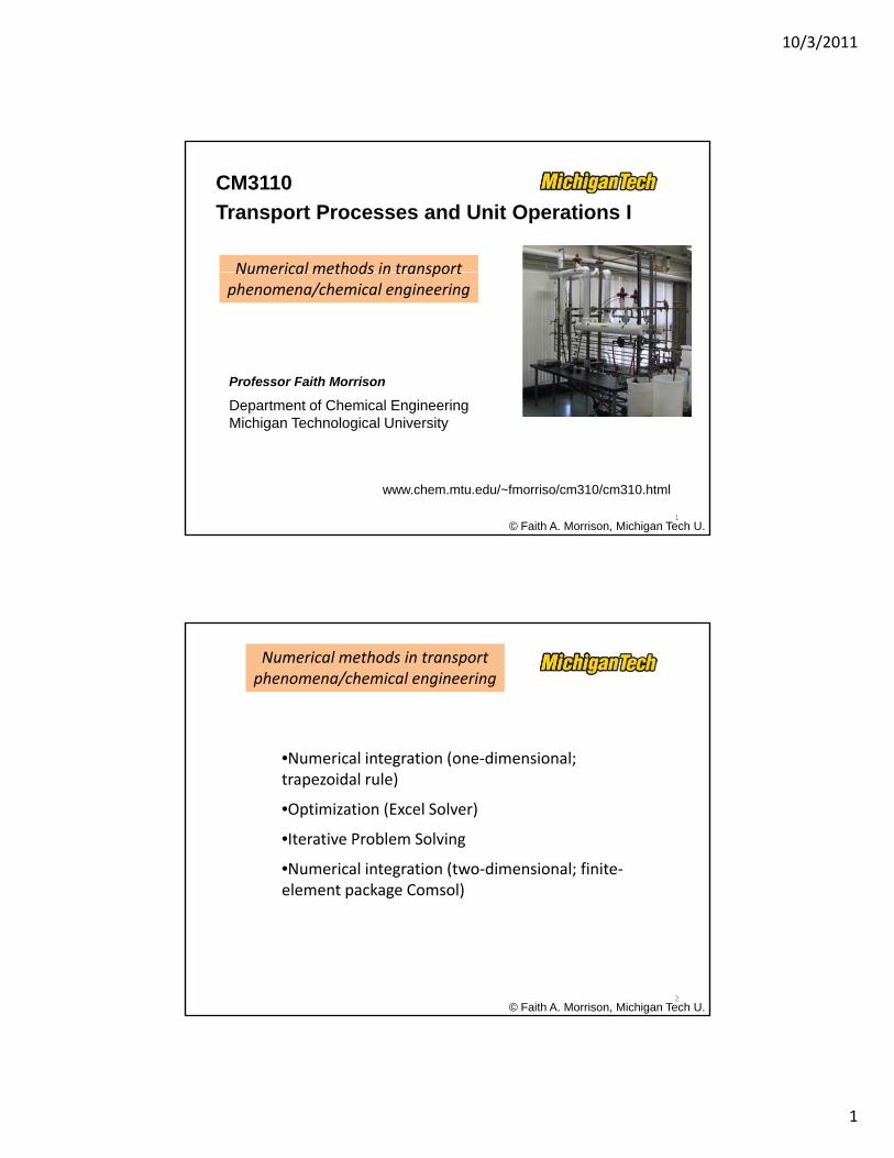
CM3110
Transport Processes and Unit Operations I
Numerical methods in transport
Professor Faith Morrison
Department of Chemical Engineering
Numerical methods in transport phenomena/chemical engineering
© Faith A. Morrison, Michigan Tech U.
Department of Chemical EngineeringMichigan Technological University
www.chem.mtu.edu/~fmorriso/cm310/cm310.html
1
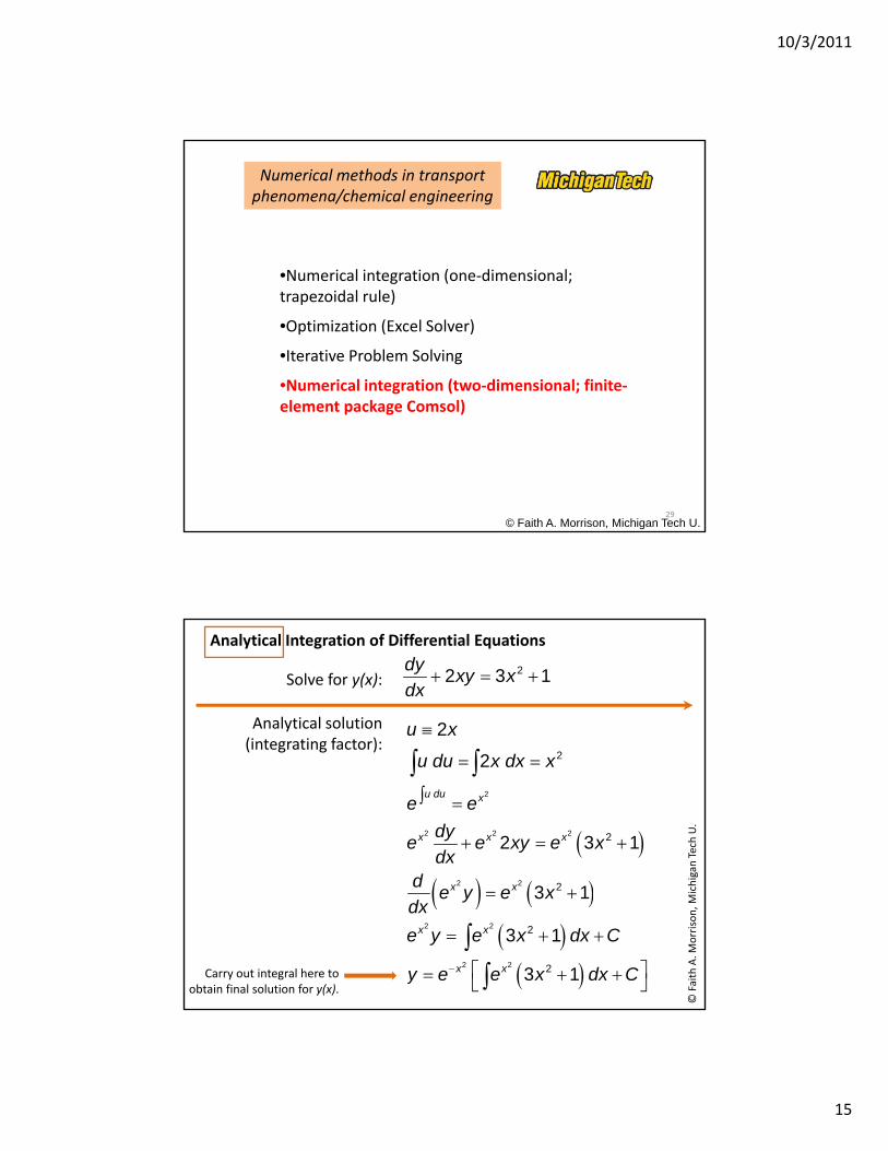
Numerical methods in transport phenomena/chemical engineering
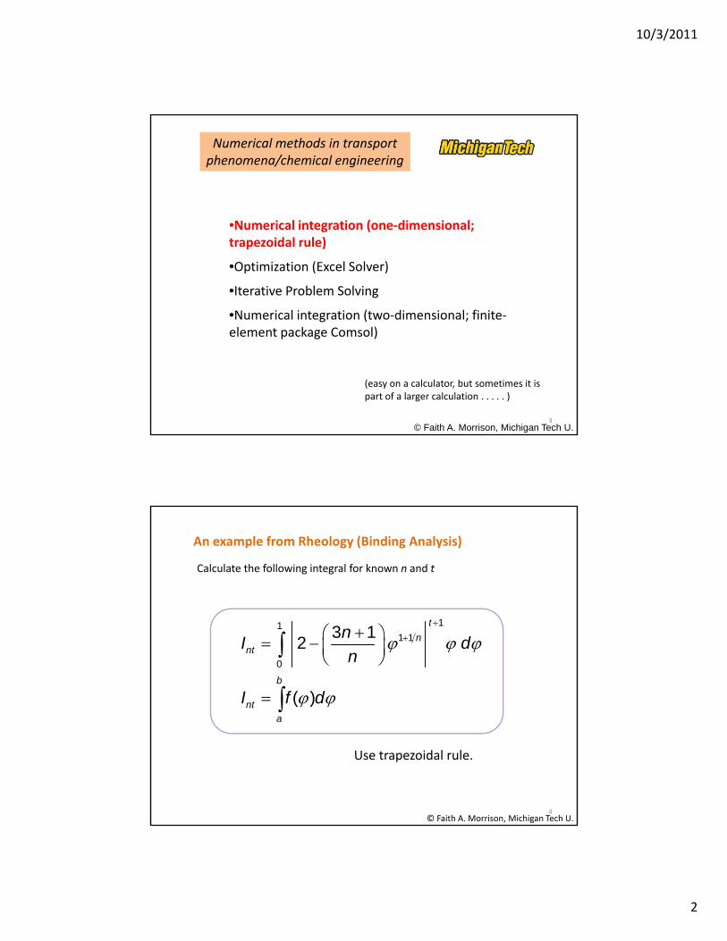
N i l i i ( di i l•Numerical integration (one‐dimensional; trapezoidal rule)
•Optimization (Excel Solver)
•Iterative Problem Solving
•Numerical integration (two‐dimensional; finite‐l k C l)
© Faith A. Morrison, Michigan Tech U.2
element package Comsol)
10/3/2011
2
Numerical methods in transport phenomena/chemical engineering
N i l i t ti ( di i l•Numerical integration (one‐dimensional; trapezoidal rule)
•Optimization (Excel Solver)
•Iterative Problem Solving
•Numerical integration (two‐dimensional; finite‐l k C l)
© Faith A. Morrison, Michigan Tech U.3
element package Comsol)
(easy on a calculator, but sometimes it is part of a larger calculation . . . . . )
An example from Rheology (Binding Analysis)
Calculate the following integral for known n and t
111 1
0
3 12
( )
t
nnt
b
nt
a
nI d
n
I f d
4
a
© Faith A. Morrison, Michigan Tech U.
Use trapezoidal rule.
10/3/2011
3
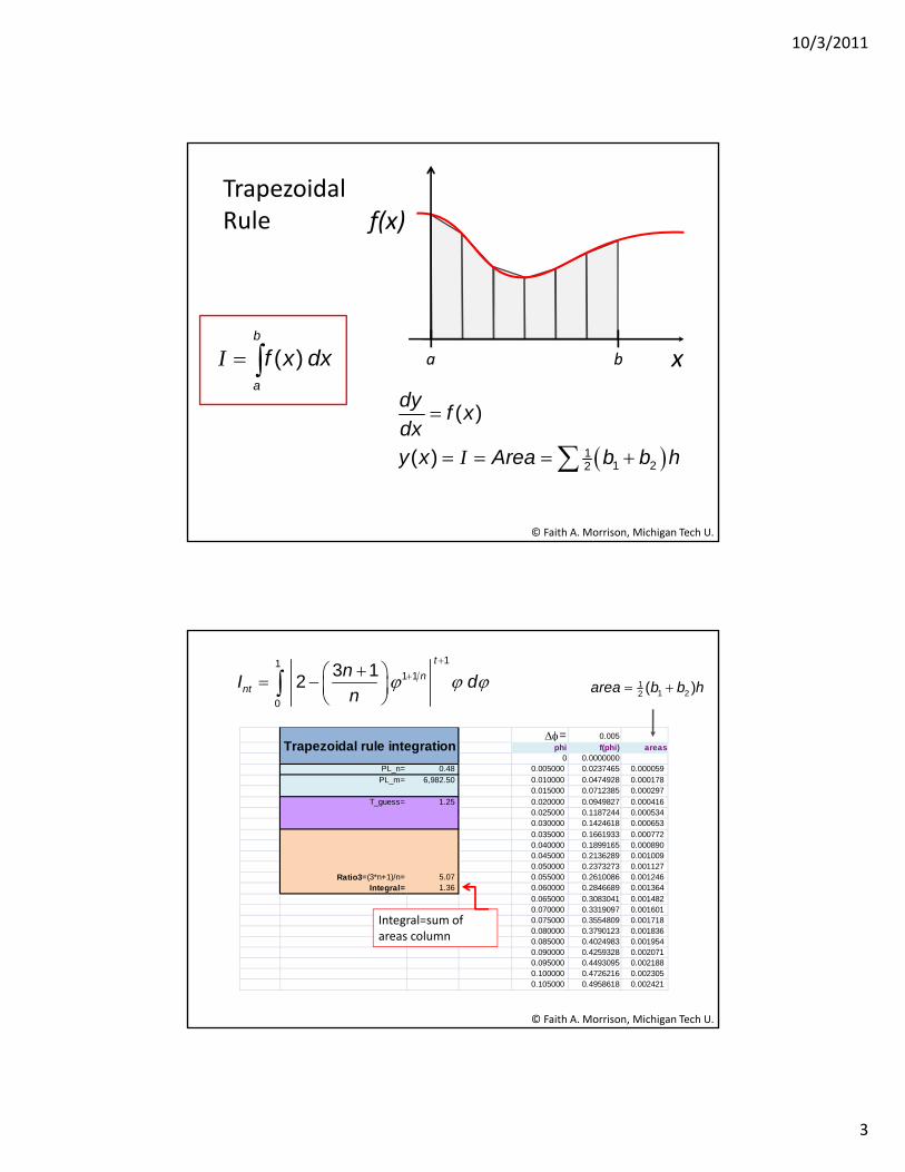
Trapezoidal Rule f(x)
a b
( )dy
f
x( )b
a
f x dx I
© Faith A. Morrison, Michigan Tech U.
11 22
( )
( )
yf x
dxy x Area b b h
I
= 0.005
phi f(phi) areas0 0.0000000
Trapezoidal rule integration
111 1
0
3 12
t
nnt
nI d
n
11 22 ( )area b b h
PL_n= 0.48 0.005000 0.0237465 0.000059 PL_m= 6,982.50 0.010000 0.0474928 0.000178
0.015000 0.0712385 0.000297 T_guess= 1.25 0.020000 0.0949827 0.000416
0.025000 0.1187244 0.000534 0.030000 0.1424618 0.000653 0.035000 0.1661933 0.000772 0.040000 0.1899165 0.000890 0.045000 0.2136289 0.001009 0.050000 0.2373273 0.001127
Ratio3=(3*n+1)/n= 5.07 0.055000 0.2610086 0.001246 Integral= 1.36 0.060000 0.2846689 0.001364
© Faith A. Morrison, Michigan Tech U.
0.065000 0.3083041 0.001482 0.070000 0.3319097 0.001601 0.075000 0.3554809 0.001718 0.080000 0.3790123 0.001836 0.085000 0.4024983 0.001954 0.090000 0.4259328 0.002071 0.095000 0.4493095 0.002188 0.100000 0.4726216 0.002305 0.105000 0.4958618 0.002421
Integral=sum of areas column
10/3/2011
4
Numerical methods in transport phenomena/chemical engineering
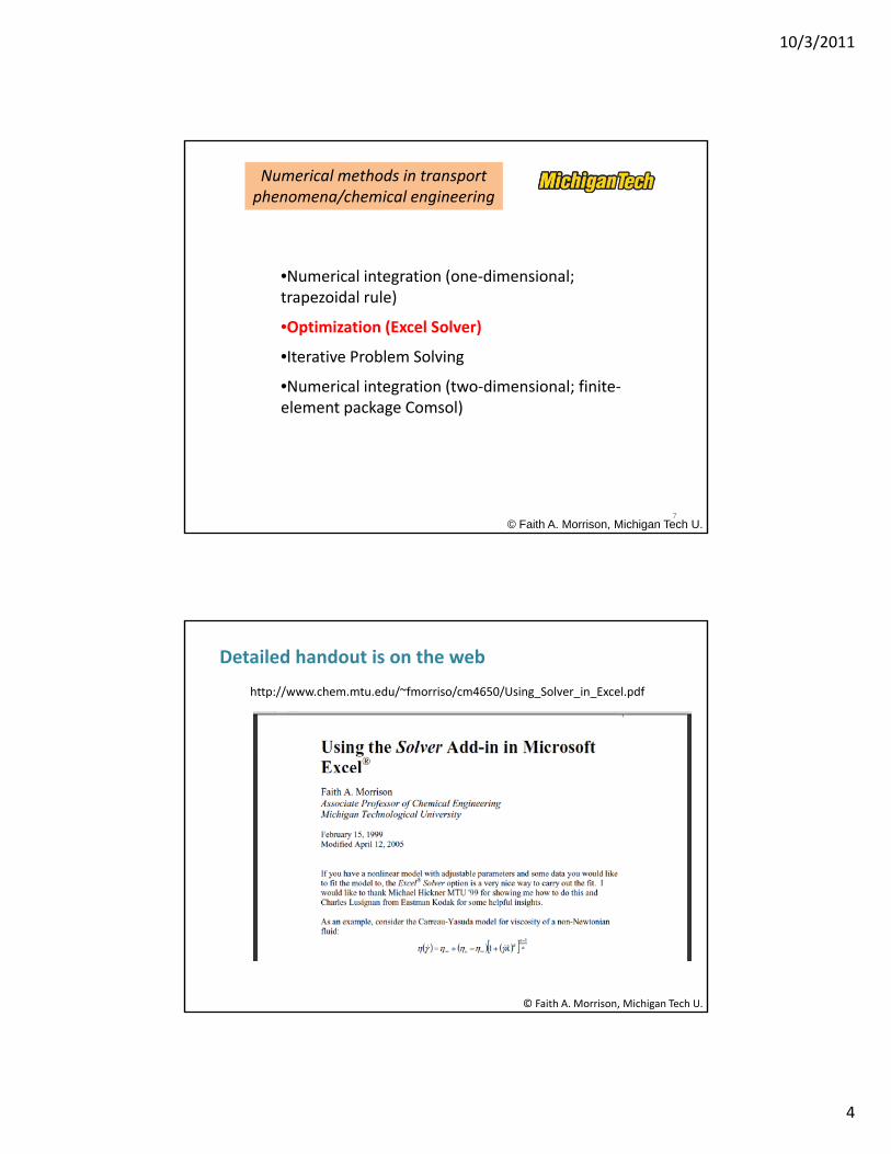
N i l i i ( di i l•Numerical integration (one‐dimensional; trapezoidal rule)
•Optimization (Excel Solver)
•Iterative Problem Solving
•Numerical integration (two‐dimensional; finite‐l k C l)
© Faith A. Morrison, Michigan Tech U.7
element package Comsol)
http://www.chem.mtu.edu/~fmorriso/cm4650/Using_Solver_in_Excel.pdf
Detailed handout is on the web
© Faith A. Morrison, Michigan Tech U.
10/3/2011
5
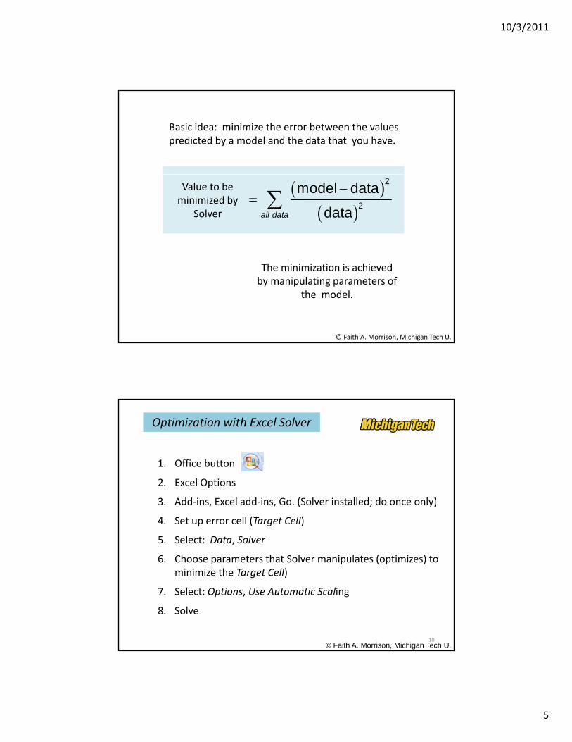
Basic idea: minimize the error between the values predicted by a model and the data that you have.
2
2
model data
dataall data
Value to be minimized by
Solver
© Faith A. Morrison, Michigan Tech U.
The minimization is achieved by manipulating parameters of
the model.
Optimization with Excel Solver
1. Office button
2 Excel Options2. Excel Options
3. Add‐ins, Excel add‐ins, Go. (Solver installed; do once only)
4. Set up error cell (Target Cell)
5. Select: Data, Solver
6. Choose parameters that Solver manipulates (optimizes) to
© Faith A. Morrison, Michigan Tech U.10
minimize the Target Cell)
7. Select: Options, Use Automatic Scaling
8. Solve
10/3/2011
6
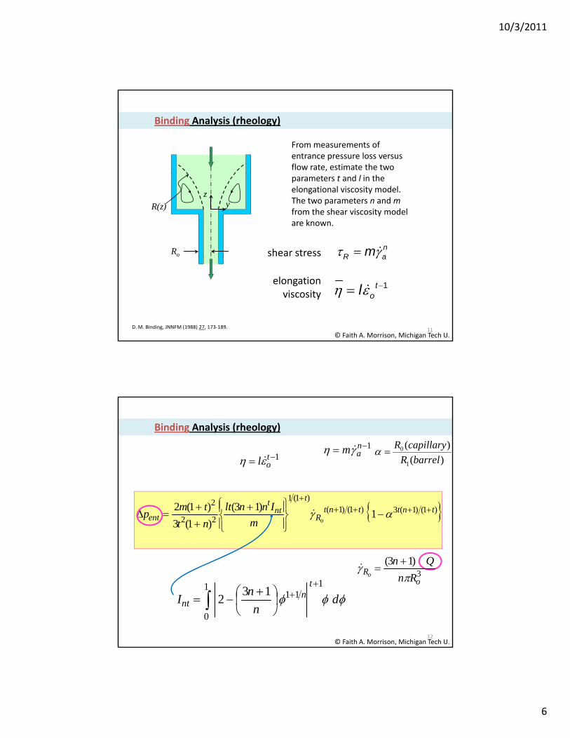
Binding Analysis (rheology)
From measurements of entrance pressure loss versus flow rate, estimate the two
Ro
y z
R(z)
nR am
parameters t and l in the elongational viscosity model. The two parameters n and mfrom the shear viscosity model are known.
shear stress
11
R a
D. M. Binding, JNNFM (1988) 27, 173‐189.
© Faith A. Morrison, Michigan Tech U.
elongation viscosity
1tol
Binding Analysis (rheology)
1 nam
1 tol )(
)(
1
0
barrelR
capillaryR
)1()1(3)1()1()1(1
22
2
1)13(
)1(3
)1(2 tnttntR
t
ntt
ent om
Innlt
nt
tmp
)13( Qn
12
1
0
11113
2 dn
nI
tn
nt
3)13(
oR
Rn
Qno
© Faith A. Morrison, Michigan Tech U.
10/3/2011
7
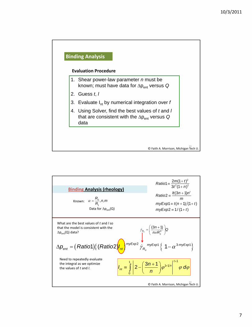
Binding Analysis
Evaluation Procedure
1. Shear power-law parameter n must be known; must have data for pent versus Q
2. Guess t, l
3. Evaluate Int by numerical integration over f
4. Using Solver, find the best values of t and l
13© Faith A. Morrison, Michigan Tech U.
that are consistent with the pent versus Qdata
Binding Analysis (rheology)
2
2 2
2 (1 )1
3 (1 )
(3 1)2
1 ( 1) (1 )
2 1/ (1 )
t
m tRatio
t n
lt n nRatio
mmyExp t n t
myExp t
0
1
, ,R
n mR
Known:
Data for pent(Q)
3
(3 1)oR
o
nQ
n R
2 1 3 11 ( 2) 1o
myExp myExp myExpent nt Rp Ratio Ratio I
What are the best values of t and l so that the model is consistent with the pent(Q) data?
14
111 1
0
3 12
t
nnt
nI d
n
© Faith A. Morrison, Michigan Tech U.
oe t t
Need to repeatedly evaluate the integral as we optimize the values of t and l.
10/3/2011
8
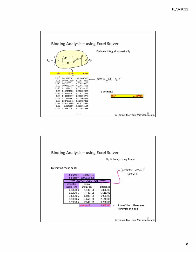
Binding Analysis – using Excel Solver
Evaluate integral numerically
1 1
11132 d
nI
tn
0
112 dn
I nnt
hbbarea )(2
121
phi f(phi) areas0 0
0.005 0.023746502 5.93663E-050.01 0.047492829 0.000178098
0.015 0.071238512 0.0002968280.02 0.094982739 0.000415553
0 025 0 118724352 0 000534268
15© Faith A. Morrison, Michigan Tech U.
. . .
Summing:
Int= 1.36055
0.025 0.118724352 0.0005342680.03 0.142461832 0.000652965
0.035 0.166193303 0.0007716380.04 0.189916517 0.000890275
0.045 0.213628861 0.0010088630.05 0.237327345 0.001127391
0.055 0.261008606 0.001245840.06 0.2846689 0.001364194
0.065 0.308304107 0.001482433
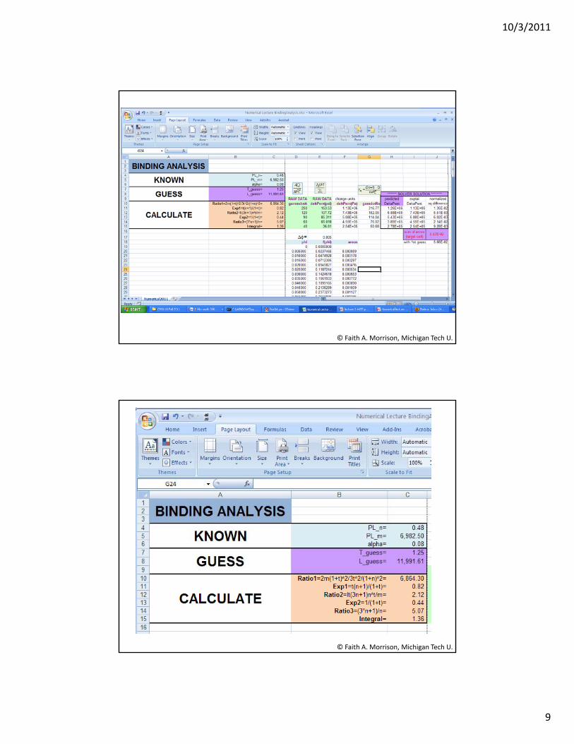
Binding Analysis – using Excel Solver
Optimize t, l using Solver
t_guess= 1.2477157l_guess= 11991.60895
predicted exptalDeltaPent DeltaPent difference
1.26E+06 1.13E+06 1.35E-026 88E+05 7 43E+05 5 51E-03
******* SOLVER SOLUTION ********
2
2
actual
actualpredicted By varying these cells:
16
6.88E 05 7.43E 05 5.51E 035.43E+05 5.88E+05 6.02E-033.89E+05 4.55E+05 2.14E-022.78E+05 2.54E+05 9.28E-03
target cell 5.57E-02
© Faith A. Morrison, Michigan Tech U.
Sum of the differences:Minimize this cell
10/3/2011
9
© Faith A. Morrison, Michigan Tech U.
© Faith A. Morrison, Michigan Tech U.
10/3/2011
10
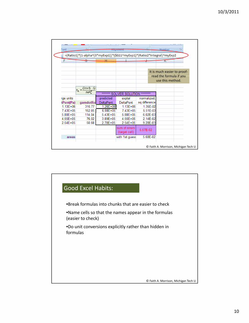
It is much easier to proof‐read the formula if youread the formula if you
use this method.
© Faith A. Morrison, Michigan Tech U.
Good Excel Habits:
•Break formulas into chunks that are easier to check
•Name cells so that the names appear in the formulas (easier to check)
•Do unit conversions explicitly rather than hidden in formulas
© Faith A. Morrison, Michigan Tech U.
10/3/2011
11
Numerical methods in transport phenomena/chemical engineering
N i l i i ( di i l•Numerical integration (one‐dimensional; trapezoidal rule)
•Optimization (Excel Solver)
•Iterative Problem Solving
•Numerical integration (two‐dimensional; finite‐l k C l)
© Faith A. Morrison, Michigan Tech U.21
element package Comsol)
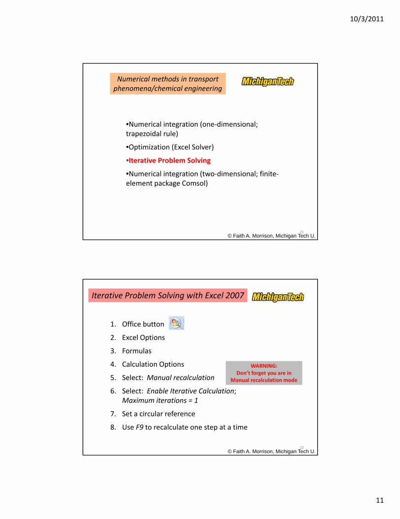
Iterative Problem Solving with Excel 2007
1. Office button
2 Excel Options2. Excel Options
3. Formulas
4. Calculation Options
5. Select: Manual recalculation
6. Select: Enable Iterative Calculation;
WARNING: Don’t forget you are in
Manual recalculation mode
© Faith A. Morrison, Michigan Tech U.22
Maximum iterations = 1
7. Set a circular reference
8. Use F9 to recalculate one step at a time
10/3/2011
12
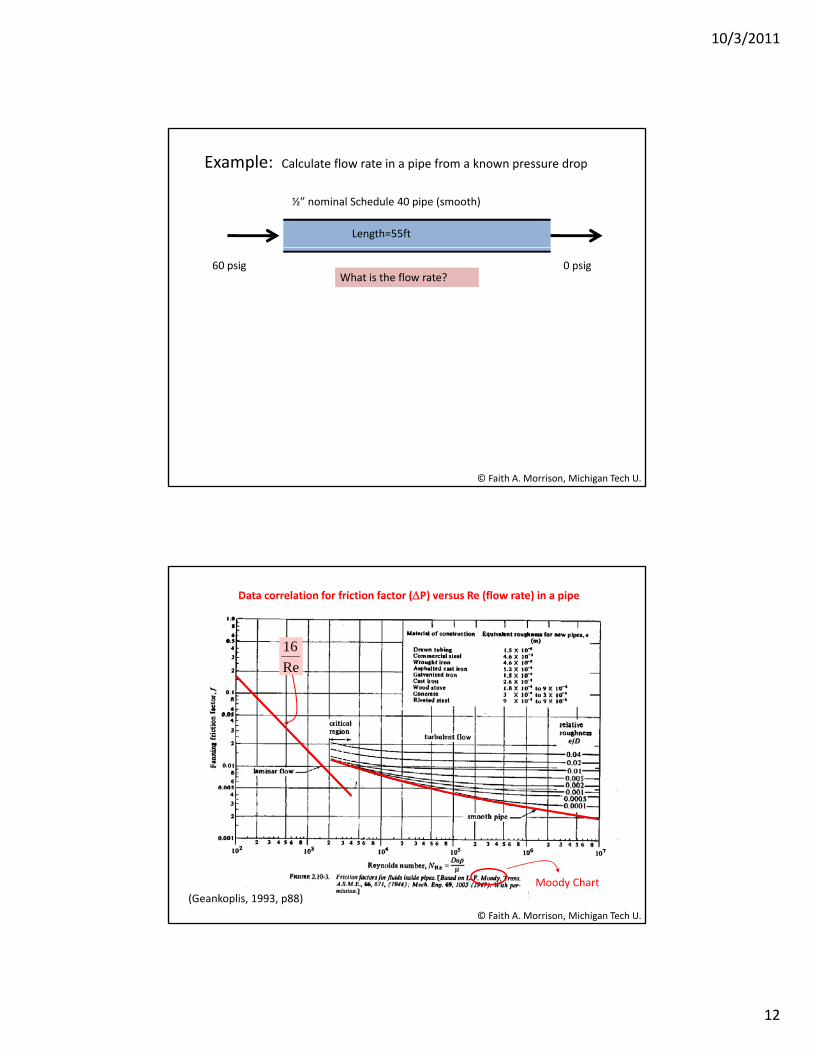
Example: Calculate flow rate in a pipe from a known pressure drop
Length=55ft
½” nominal Schedule 40 pipe (smooth)
60 psig 0 psigWhat is the flow rate?
© Faith A. Morrison, Michigan Tech U.
Data correlation for friction factor (P) versus Re (flow rate) in a pipe
Re
16
(Geankoplis, 1993, p88)
© Faith A. Morrison, Michigan Tech U.
Moody Chart
10/3/2011
13
Reynolds Number
Dv velocityaveragev
densityFlow rate
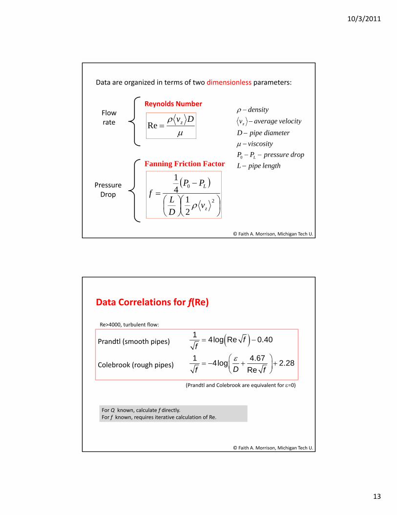
Data are organized in terms of two dimensionless parameters:
Fanning Friction Factor
DvzRe
lengthpipeL
droppressurePP
viscosity
diameterpipeD
velocityaveragev
L
z
0
rate
1
© Faith A. Morrison, Michigan Tech U.
Pressure Drop
2
0
21
41
z
L
vDL
PPf
Data Correlations for f(Re)
1Re>4000, turbulent flow:
14log Re 0.40
1 4.674log 2.28
Re
ff
Df f
Prandtl (smooth pipes)
Colebrook (rough pipes)
(Prandtl and Colebrook are equivalent for =0)
© Faith A. Morrison, Michigan Tech U.
For Q known, calculate f directly.For f known, requires iterative calculation of Re.
10/3/2011
14
density= 62.25 lbm/ft3 circular cells
viscosity= 6.01E‐04 lbm/ft.s
D= 0.622 in
D= 0.052 ft
L= 55 ftgiven
Implemented in Excel
DeltaP= 60 psi
DeltaP= 588 lbf/ft^2
Step1 Flow rate (guess)= 4.60 gpm
Flow rate= 0.0102 ft^3/s
velocity= 4.8559 ft/s
2 Re= 26,092
guess f= 0.00607
RHS Prandtl 12 83 error
© Faith A. Morrison, Michigan Tech U.
RHS Prandtl= 12.83 error=
3 new_f= 0.00607 0.000%
4 velocity_second= 4.86 ft/s
Q_new= 0.0102 ft^3/s
5 Q_new= 4.60 gpm
Alternative (but more complex) correlation; no iteration on f required (F. A. Morrison, 2011)
Flow in smooth pipes: (all Reynolds numbers)
0.165
7.0
31700.0076
16ReRe3170
1Re
f
© Faith A. Morrison, Michigan Tech U.
(would still need to iterate on Q if used in our problem)
10/3/2011
15
Numerical methods in transport phenomena/chemical engineering
N i l i i ( di i l•Numerical integration (one‐dimensional; trapezoidal rule)
•Optimization (Excel Solver)
•Iterative Problem Solving
•Numerical integration (two‐dimensional; finite‐l t k C l)
© Faith A. Morrison, Michigan Tech U.29
element package Comsol)
Analytical Integration of Differential Equations
22 3 1dy
xy xdx
Solve for y(x):
2u x
Analytical solution (integrating factor):
igan
Tech U.
2
2 2 2
2
2
2
2 3 1
u du x
x x x
u du x dx x
e e
dye e xy e x
dxd
(integrating factor):
© Faith A. M
orrison, M
ich
2 2
2 2
2 2
2
2
2
3 1
3 1
3 1
x x
x x
x x
de y e x
dx
e y e x dx C
y e e x dx C
Carry out integral here to
obtain final solution for y(x).
10/3/2011
16
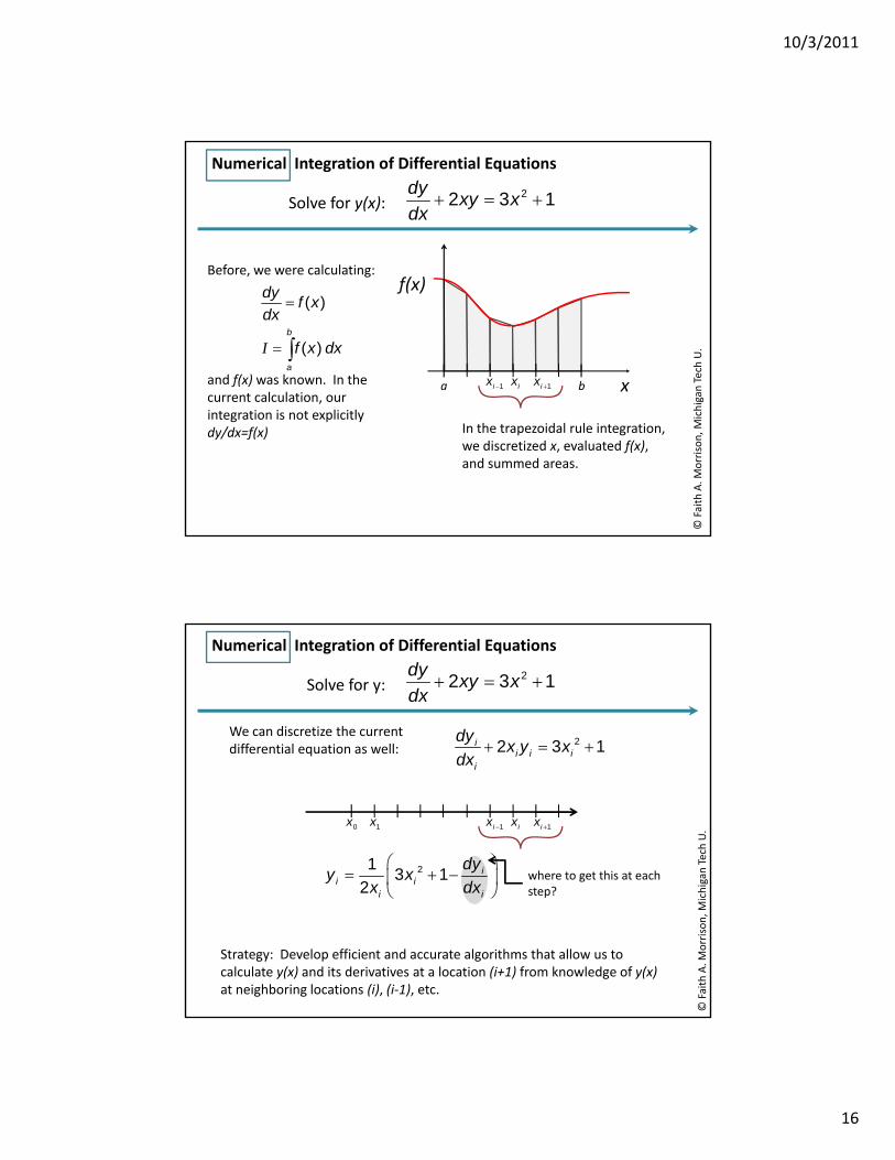
Numerical Integration of Differential Equations
22 3 1dy
xy xdx
Solve for y(x):
Before we were calculating:
igan
Tech U.
Before, we were calculating:
( )
( )b
a
dyf x
dx
f x dx
I
and f(x) was known. In the current calculation, our
a b
f(x)
xix 1ix 1ix
© Faith A. M
orrison, M
ich
integration is not explicitly dy/dx=f(x) In the trapezoidal rule integration,
we discretized x, evaluated f(x), and summed areas.
Numerical Integration of Differential Equations
22 3 1dy
xy xdx
Solve for y:
We can discretize the current differential equation as well:
22 3 1ii i i
dyx y x
d
igan
Tech U.
q i i ii
ydx
ix 1ix 1ix 0x 1x
213 1
2i
i i
dyy x
x dx
where to get this at each
?
© Faith A. M
orrison, M
ich
Strategy: Develop efficient and accurate algorithms that allow us to calculate y(x) and its derivatives at a location (i+1) from knowledge of y(x) at neighboring locations (i), (i‐1), etc.
2 i ix dx step?
10/3/2011
17
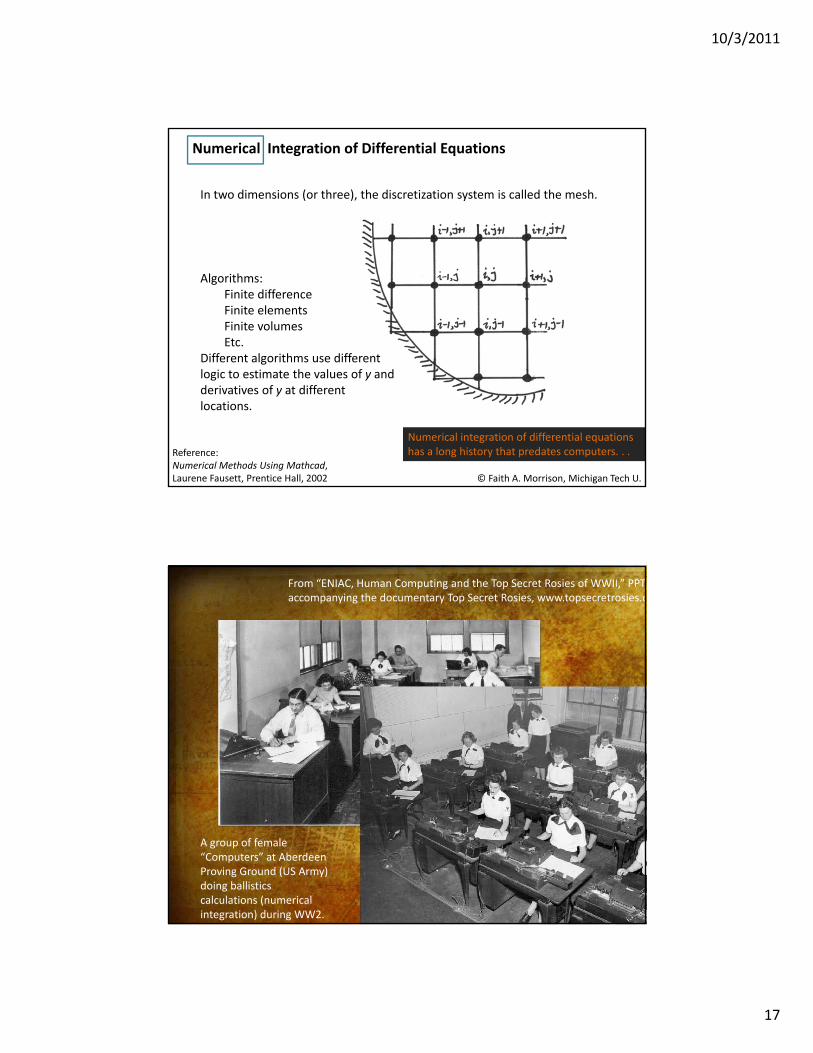
Numerical Integration of Differential Equations
In two dimensions (or three), the discretization system is called the mesh.
Algorithms:Finite differenceFinite elementsFinite volumesEtc.
Different algorithms use different
© Faith A. Morrison, Michigan Tech U.
logic to estimate the values of y and derivatives of y at different locations.
Reference: Numerical Methods Using Mathcad, Laurene Fausett, Prentice Hall, 2002
Numerical integration of differential equations has a long history that predates computers. . .
From “ENIAC, Human Computing and the Top Secret Rosies of WWII,” PPT accompanying the documentary Top Secret Rosies, www.topsecretrosies.c
© Faith A. Morrison, Michigan Tech U.
A group of female “Computers” at Aberdeen Proving Ground (US Army) doing ballisticscalculations (numerical integration) during WW2.
10/3/2011
18
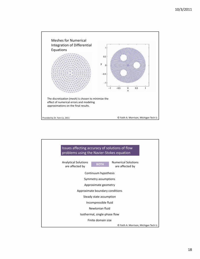
Meshes for Numerical Integration of Differential Equations
© Faith A. Morrison, Michigan Tech U.Provided by Dr. Tom Co, 2011
The discretization (mesh) is chosen to minimize the effect of numerical errors and modeling approximations on the final results.
Issues affecting accuracy of solutions of flow problems using the Navier‐Stokes equation
Analytical Solutions are affected by
Numerical Solutions are affected by
BOTH
Continuum hypothesis
Symmetry assumptions
Approximate geometry
Approximate boundary conditions
Steady state assumption
© Faith A. Morrison, Michigan Tech U.
y p
Incompressible fluid
Newtonian fluid
Isothermal, single‐phase flow
Finite domain size
10/3/2011
19
Issues affecting accuracy of solutions of flow problems using the Navier‐Stokes equation
Analytical Solutions are affected by
Numerical Solutions are affected by
Neglect inconvenient terms
Linearization and other approximate analytical solution
methods
Final solution series truncation
Discretization of flow domain
Derivative approximations
Round‐off error
Interpolation error in final engineering quantities
© Faith A. Morrison, Michigan Tech U.
errorg g q
Numerical instability induced by accumulation of error
Inappropriate implementation of commercial code
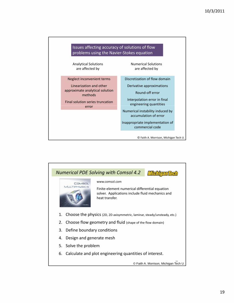
Numerical PDE Solving with Comsol 4.2
www.comsol.com
Finite‐element numerical differential equation solver. Applications include fluid mechanics and h t t f
1. Choose the physics (2D, 2D axisymmetric, laminar, steady/unsteady, etc.)
2. Choose flow geometry and fluid (shape of the flow domain)
3. Define boundary conditions
heat transfer.
© Faith A. Morrison, Michigan Tech U.38
y
4. Design and generate mesh
5. Solve the problem
6. Calculate and plot engineering quantities of interest.
10/3/2011
20
Comsol Multiphysics 4.2 0Launch the program
© Faith A. Morrison, Michigan Tech U.
Comsol Multiphysics 4.2 0Launch the program
© Faith A. Morrison, Michigan Tech U.

10/3/2011
21
Comsol Multiphysics 4.2 0Launch the program
© Faith A. Morrison, Michigan Tech U.
Comsol Multiphysics 4.2 1Choose the physics
© Faith A. Morrison, Michigan Tech U.
10/3/2011
22
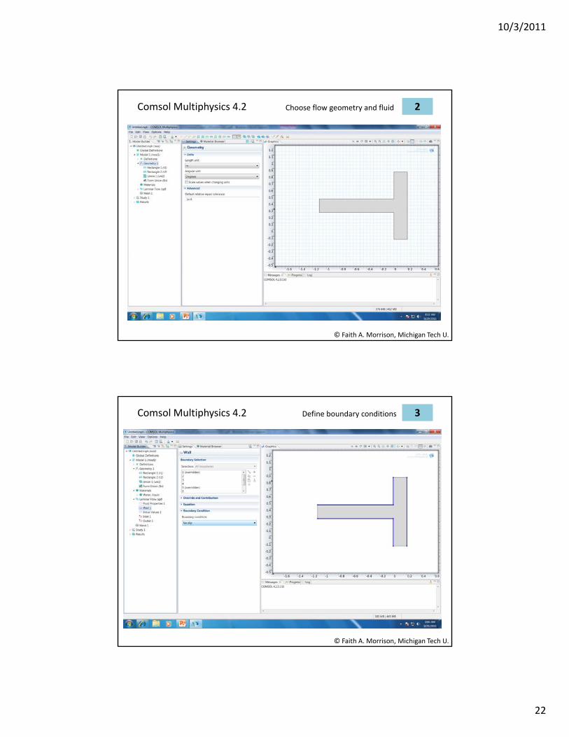
Comsol Multiphysics 4.2 2Choose flow geometry and fluid
© Faith A. Morrison, Michigan Tech U.
Comsol Multiphysics 4.2 3Define boundary conditions
© Faith A. Morrison, Michigan Tech U.
10/3/2011
23
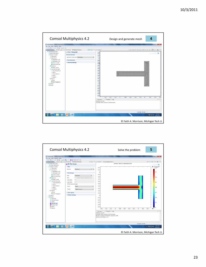
Comsol Multiphysics 4.2 4Design and generate mesh
© Faith A. Morrison, Michigan Tech U.
Comsol Multiphysics 4.2 5Solve the problem
© Faith A. Morrison, Michigan Tech U.
10/3/2011
24
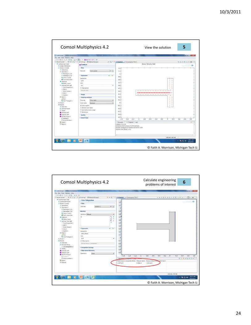
Comsol Multiphysics 4.2 5View the solution
© Faith A. Morrison, Michigan Tech U.
Comsol Multiphysics 4.2 6Calculate engineering problems of interest
© Faith A. Morrison, Michigan Tech U.
10/3/2011
25
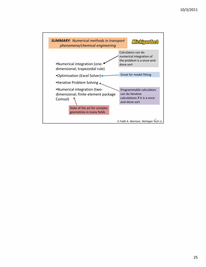
SUMMARY: Numerical methods in transport phenomena/chemical engineering
N i l i i (
Calculators can do numerical integration of the problem is a once‐and‐
•Numerical integration (one‐dimensional; trapezoidal rule)
•Optimization (Excel Solver)
•Iterative Problem Solving
•Numerical integration (two‐di i l fi i l k
done sort
Programmable calculators d it ti
Great for model fitting
© Faith A. Morrison, Michigan Tech U.49
dimensional; finite‐element package Comsol)
can do iterative calculations if it is a once‐and‐done sort
State of the art for complex geometries in many fields