CME 345: MODEL REDUCTION - web.stanford.edu€¦ · CME 345: MODEL REDUCTION - Balanced Truncation Reachability and Observability Systems Considered Consider the following stable

CME 345: MODEL REDUCTION - Balanced Truncation

CME 345: MODEL REDUCTIONBalanced Truncation

Charbel Farhat & David AmsallemStanford University

[email protected]

These slides are based on the recommended textbook: A.C. Antoulas, “Approximation ofLarge-Scale Dynamical Systems,” Advances in Design and Control, SIAM,

ISBN-0-89871-529-6

1 / 42


Outline

1 Reachability and Observability

2 Balancing

3 Balanced Truncation Method

4 Error Analysis

5 Stability Analysis

6 Computational Complexity

7 Comparison with the POD Method

8 Application

9 Balanced POD Method

2 / 42


Reachability and Observability

Systems Considered

Consider the following stable LTI high-dimensional system

d

dtw(t) = Aw(t) + Bu(t)

y(t) = Cw(t)

w(0) = w0

w ∈ RN : State variablesu ∈ Rp: Input variables, typically p � Ny ∈ Rq: Output variables, typically q � N

Recall that the solution w(t) of the above linear ODE can bewritten as

w(t) = φ(t,u; t0,w0) = eA(t−t0)w(t0)+

∫ t

t0

eA(t−τ)Bu(τ)dτ, ∀t ≥ t0

3 / 42



Reachability, Controllability and Observability

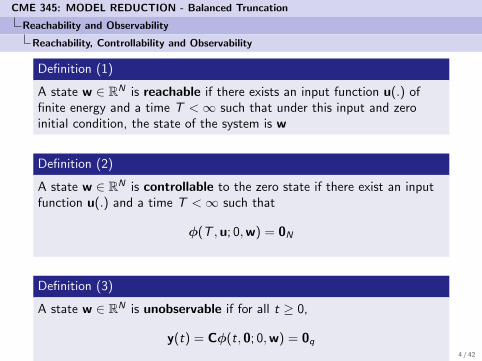
Definition (1)

A state w ∈ RN is reachable if there exists an input function u(.) offinite energy and a time T <∞ such that under this input and zeroinitial condition, the state of the system is w

Definition (2)

A state w ∈ RN is controllable to the zero state if there exist an inputfunction u(.) and a time T <∞ such that

φ(T ,u; 0,w) = 0N

Definition (3)

A state w ∈ RN is unobservable if for all t ≥ 0,

y(t) = Cφ(t, 0; 0,w) = 0q

4 / 42



Completely Controllable Dynamical System

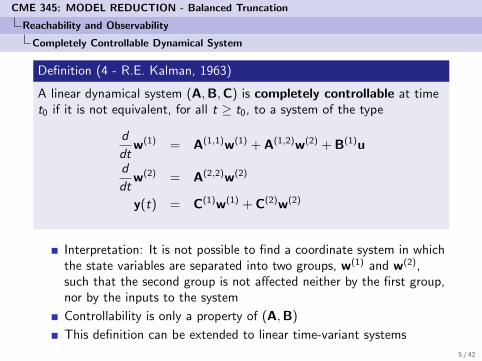
Definition (4 - R.E. Kalman, 1963)

A linear dynamical system (A,B,C) is completely controllable at timet0 if it is not equivalent, for all t ≥ t0, to a system of the type

d

dtw(1) = A(1,1)w(1) + A(1,2)w(2) + B(1)u

d

dtw(2) = A(2,2)w(2)

y(t) = C(1)w(1) + C(2)w(2)

Interpretation: It is not possible to find a coordinate system in whichthe state variables are separated into two groups, w(1) and w(2),such that the second group is not affected neither by the first group,nor by the inputs to the system

Controllability is only a property of (A,B)

This definition can be extended to linear time-variant systems

5 / 42



Completely Observable Dynamical System

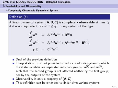
Definition (5)

A linear dynamical system (A,B,C) is completely observable at time t0if it is not equivalent, for all t ≤ t0, to any system of the type

d

dtw(1) = A(1,1)w(1) + B(1)u

d

dtw(2) = A(2,1)w(1) + A(2,2)w(2) + B(2)u

y(t) = C(1)w(1)

Dual of the previous definitionInterpretation: It is not possible to find a coordinate system in whichthe state variables are separated into two groups, w(1) and w(2),such that the second group is not affected neither by the first group,nor by the outputs of the systemObservability is only a property of (A,C)This definition can be extended to linear time-variant systems

6 / 42



Example: Simple RLC Circuit

_

+

u1

y1

w1

w2

R = 1 R = 1

L

C

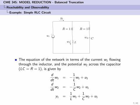
The equation of the network in terms of the current w1 flowingthrough the inductor, and the potential w2 across the capacitor(LC = R = 1), is given by

d

dtw1 = −1

Lw1 + u1

d

dtw2 = − 1

Cw2 + u1

y1 =1

Lw1 +

1

Cw2 + u1

7 / 42



Example: Simple RLC Circuit

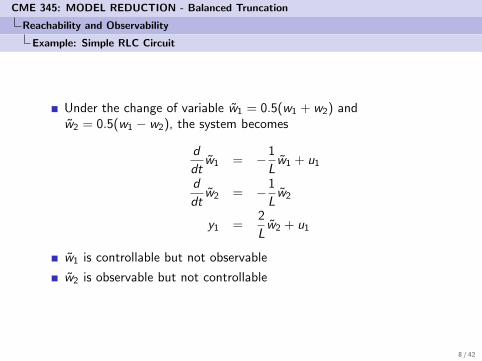
Under the change of variable w1 = 0.5(w1 + w2) andw2 = 0.5(w1 − w2), the system becomes

d

dtw1 = −1

Lw1 + u1

d

dtw2 = −1

Lw2

y1 =2

Lw2 + u1

w1 is controllable but not observable

w2 is observable but not controllable

8 / 42



Canonical Structure Theorem

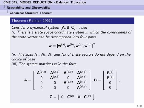
Theorem (Kalman 1961)

Consider a dynamical system (A,B,C). Then(i) There is a state space coordinate system in which the components ofthe state vector can be decomposed into four parts

w = [w(a),w(b),w(c),w(d)]T

(ii) The sizes Na, Nb, Nc and Nd of these vectors do not depend on thechoice of basis(iii) The system matrices take the form

A =

A(a,a) A(a,b) A(a,c) A(a,d)

0 A(b,b) 0 A(b,d)

0 0 A(c,c) A(c,d)

0 0 0 A(d,d)

,B =

B(a)

B(b)

00

,C =

[0 C(b) 0 C(d)

]9 / 42



Canonical Structure Theorem

The four parts of w can be interpreted as follows

Part (a) is completely controllable but unobservablePart (b) is completely controllable and completely observablePart (c) is uncontrollable and unobservablePart (d) is uncontrollable and completely observable

This theorem can be extended to linear time-variant systems

10 / 42



Reachable and Controllable Subspaces

Definition (6)

The reachable subspace Wreach ⊂ RN of a system (A,B,C) is the setcontaining all of the reachable states of the system.

R(A,B) = [B,AB, · · · ,AN−1B, · · · ]

is the reachability matrix of the system.

Definition (7)

The controllable subspace Wcontr ⊂ RN of a system (A,B,C) is the setcontaining all of the controllable states of the system

11 / 42



Reachable and Controllable Subspaces

Theorem

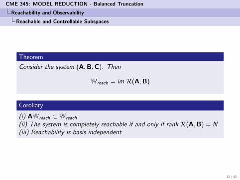
Consider the system (A,B,C). Then

Wreach = im R(A,B)

Corollary

(i) AWreach ⊂Wreach

(ii) The system is completely reachable if and only if rank R(A,B) = N(iii) Reachability is basis independent

12 / 42



Reachability and Observability Gramians

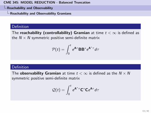
Definition

The reachability (controllability) Gramian at time t <∞ is defined asthe N × N symmetric positive semi-definite matrix

P(t) =

∫ t

0

eAτBB∗eA∗τdτ

Definition

The observability Gramian at time t <∞ is defined as the N × Nsymmetric positive semi-definite matrix

Q(t) =

∫ t

0

eA∗τC∗CeAτdτ

13 / 42



Reachability and Observability Gramians

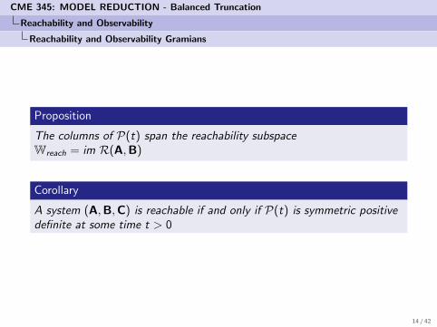
Proposition

The columns of P(t) span the reachability subspaceWreach = im R(A,B)

Corollary

A system (A,B,C) is reachable if and only if P(t) is symmetric positivedefinite at some time t > 0

14 / 42



Equivalence Between Reachability and Controllability

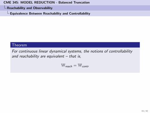
Theorem

For continuous linear dynamical systems, the notions of controllabilityand reachability are equivalent – that is,

Wreach = Wcontr

15 / 42



Unobservability Subspace

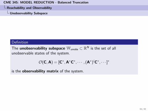
Definition

The unobservability subspace Wunobs ⊂ RN is the set of allunobservable states of the system.

O(C,A) = [C∗,A∗C∗, · · · , (A∗)iC∗, · · · ]∗

is the observability matrix of the system.

16 / 42



Unobservability Subspace

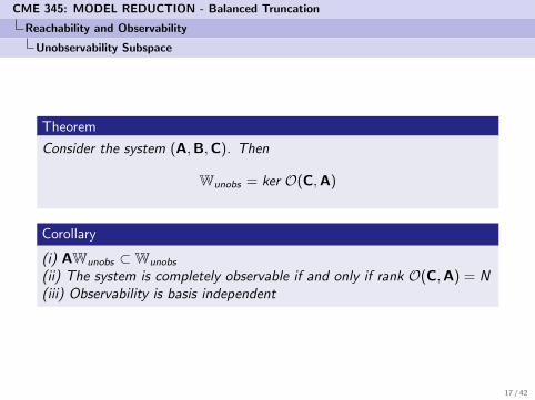
Theorem

Consider the system (A,B,C). Then

Wunobs = ker O(C,A)

Corollary

(i) AWunobs ⊂Wunobs

(ii) The system is completely observable if and only if rank O(C,A) = N(iii) Observability is basis independent

17 / 42



Infinite Gramians

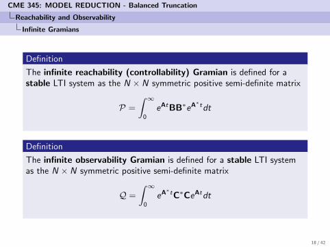
Definition

The infinite reachability (controllability) Gramian is defined for astable LTI system as the N × N symmetric positive semi-definite matrix

P =

∫ ∞0

eAtBB∗eA∗tdt

Definition

The infinite observability Gramian is defined for a stable LTI systemas the N × N symmetric positive semi-definite matrix

Q =

∫ ∞0

eA∗tC∗CeAtdt

18 / 42



Infinite Gramians

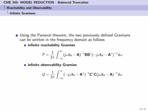
Using the Parseval theorem, the two previously defined Gramianscan be written in the frequency domain as follows

infinite reachability Gramian

P =1

2π

∫ ∞−∞

(jωIN − A)−1BB∗(−jωIN − A∗)−1dω

infinite observability Gramian

Q =1

2π

∫ ∞−∞

(−jωIN − A∗)−1C∗C(jωIN − A)−1dω

19 / 42



Infinite Gramians

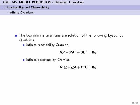
The two infinite Gramians are solution of the following Lyapunovequations

infinite reachability Gramian

AP + PA∗ + BB∗ = 0N

infinite observability Gramian

A∗Q+QA + C∗C = 0N

20 / 42



Energetic Interpretation

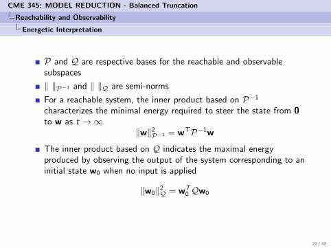
P and Q are respective bases for the reachable and observablesubspaces

‖ ‖P−1 and ‖ ‖Q are semi-norms

For a reachable system, the inner product based on P−1characterizes the minimal energy required to steer the state from 0to w as t →∞

‖w‖2P−1 = wTP−1w

The inner product based on Q indicates the maximal energyproduced by observing the output of the system corresponding to aninitial state w0 when no input is applied

‖w0‖2Q = wT0 Qw0

21 / 42


Balancing

Model Order Reduction Based on Balancing

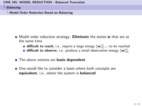
Model order reduction strategy: Eliminate the states w that are atthe same time

difficult to reach, i.e., require a large energy ‖w‖2P−1 to be reacheddifficult to observe, i.e., produce a small observation energy ‖w‖2Q

The above notions are basis dependent

One would like to consider a basis where both concepts areequivalent, i.e., where the system is balanced

22 / 42


Balancing

The Effect of Basis Change on the Gramians

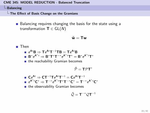
Balancing requires changing the basis for the state using atransformation T ∈ GL(N)

w = Tw

Then

eAtB⇒ TeAtT−1TB = TeAtBB∗eA∗t ⇒ B∗T∗T−∗eA∗tT∗ = B∗eA∗tT∗

the reachability Gramian becomes

P = TPT∗

CeAt ⇒ CT−1TeAtT−1 = CeAtT−1

eA∗tC∗ ⇒ T−∗eA∗tT∗T−∗C∗ = T−∗eA∗tC∗

the observability Gramian becomes

Q = T−∗QT−1

23 / 42


Balancing

Balancing Transformation

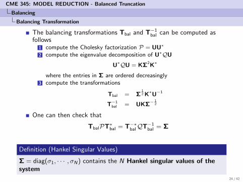
The balancing transformations Tbal and T−1bal can be computed asfollows

1 compute the Cholesky factorization P = UU∗

2 compute the eigenvalue decomposition of U∗QU

U∗QU = KΣ2K∗

where the entries in Σ are ordered decreasingly3 compute the transformations

Tbal = Σ12 K∗U−1

T−1bal = UKΣ−

12

One can then check that

TbalPT∗bal = T−∗balQT−1bal = Σ

Definition (Hankel Singular Values)

Σ = diag(σ1, · · · , σN) contains the N Hankel singular values of thesystem

24 / 42


Balancing

Variational Interpretation

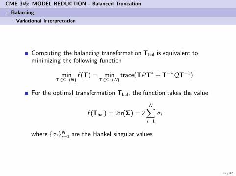
Computing the balancing transformation Tbal is equivalent tominimizing the following function

minT∈GL(N)

f (T) = minT∈GL(N)

trace(TPT∗ + T−∗QT−1)

For the optimal transformation Tbal, the function takes the value

f (Tbal) = 2tr(Σ) = 2N∑i=1

σi

where {σi}Ni=1 are the Hankel singular values

25 / 42


Balanced Truncation Method

Block Partitioning of the System

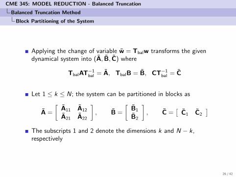
Applying the change of variable w = Tbalw transforms the givendynamical system into (A, B, C) where

TbalAT−1bal = A, TbalB = B, CT−1bal = C

Let 1 ≤ k ≤ N; the system can be partitioned in blocks as

A =

[A11 A12

A21 A22

], B =

[B1

B2

], C =

[C1 C2

]The subscripts 1 and 2 denote the dimensions k and N − k,respectively

26 / 42


Balanced Truncation Method

Block Partitioning of the System

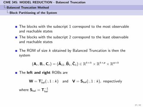
The blocks with the subscript 1 correspond to the most observableand reachable states

The blocks with the subscript 2 correspond to the least observableand reachable states

The ROM of size k obtained by Balanced Truncation is then thesystem

(Ar ,Br ,Cr ) = (A11, B1, C1) ∈ Rk×k × Rk×p × Rq×k

The left and right ROBs are

W = T∗bal(:, 1 : k) and V = Sbal(:, 1 : k), respectively

where Sbal = T−1bal

27 / 42


Error Analysis

Error Criterion

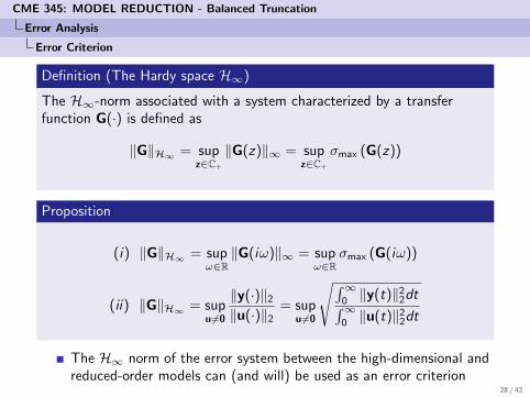
Definition (The Hardy space H∞)

The H∞-norm associated with a system characterized by a transferfunction G(·) is defined as

‖G‖H∞ = supz∈C+

‖G(z)‖∞ = supz∈C+

σmax (G(z))

Proposition

(i) ‖G‖H∞ = supω∈R‖G(iω)‖∞ = sup

ω∈Rσmax (G(iω))

(ii) ‖G‖H∞ = supu6=0

‖y(·)‖2‖u(·)‖2

= supu6=0

√∫∞0‖y(t)‖22dt∫∞

0‖u(t)‖22dt

The H∞ norm of the error system between the high-dimensional andreduced-order models can (and will) be used as an error criterion

28 / 42


Error Analysis

Theorem

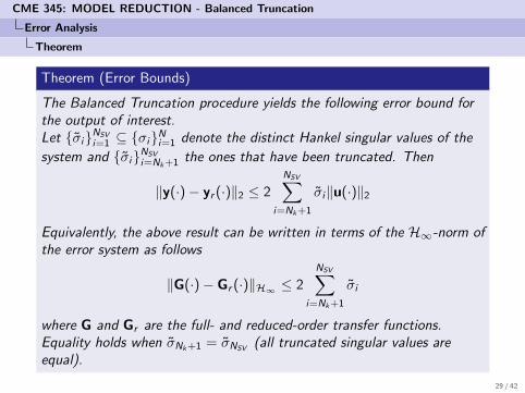
Theorem (Error Bounds)

The Balanced Truncation procedure yields the following error bound forthe output of interest.Let {σi}NSV

i=1 ⊆ {σi}Ni=1 denote the distinct Hankel singular values of the

system and {σi}NSV

i=Nk+1 the ones that have been truncated. Then

‖y(·)− yr (·)‖2 ≤ 2

NSV∑i=Nk+1

σi‖u(·)‖2

Equivalently, the above result can be written in terms of the H∞-norm ofthe error system as follows

‖G(·)− Gr (·)‖H∞ ≤ 2

NSV∑i=Nk+1

σi

where G and Gr are the full- and reduced-order transfer functions.Equality holds when σNk+1 = σNSV

(all truncated singular values areequal).

29 / 42


Error Analysis

Theorem

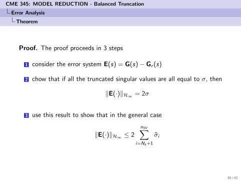
Proof. The proof proceeds in 3 steps

1 consider the error system E(s) = G(s)− Gr (s)

2 chow that if all the truncated singular values are all equal to σ, then

‖E(·)‖H∞ = 2σ

3 use this result to show that in the general case

‖E(·)‖H∞ ≤ 2

nSV∑i=Nk+1

σi

30 / 42


Stability Analysis

Theorem

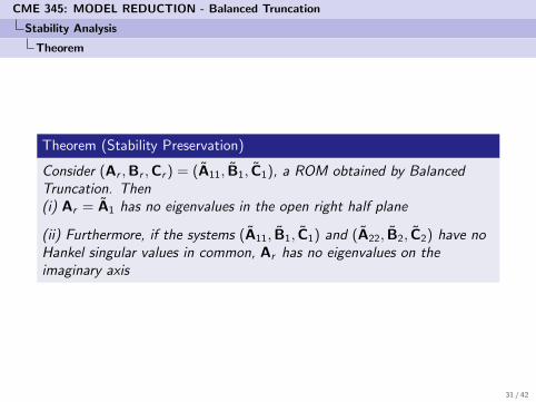
Theorem (Stability Preservation)

Consider (Ar ,Br ,Cr ) = (A11, B1, C1), a ROM obtained by BalancedTruncation. Then(i) Ar = A1 has no eigenvalues in the open right half plane

(ii) Furthermore, if the systems (A11, B1, C1) and (A22, B2, C2) have noHankel singular values in common, Ar has no eigenvalues on theimaginary axis

31 / 42


Computational Complexity

Numerical Methods

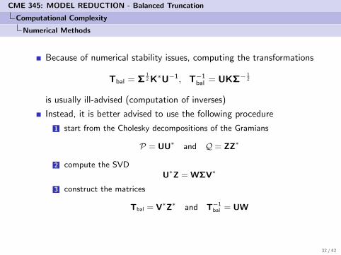
Because of numerical stability issues, computing the transformations

Tbal = Σ12 K∗U−1, T−1bal = UKΣ−

12

is usually ill-advised (computation of inverses)

Instead, it is better advised to use the following procedure

1 start from the Cholesky decompositions of the Gramians

P = UU∗ and Q = ZZ∗

2 compute the SVDU∗Z = WΣV∗

3 construct the matrices

Tbal = V∗Z∗ and T−1bal = UW

32 / 42


Computational Complexity

Cost and Limitations

Balanced Truncation leads to ROMs with quality and stabilityguarantees; however

the computation of the Gramians is expensive as it requires thesolution of a Lyapunov equation (O(N3) operations)

for this reason, Balanced Truncation is in general impractical forlarge systems of size N & 105

33 / 42


Comparison with the POD Method

POD

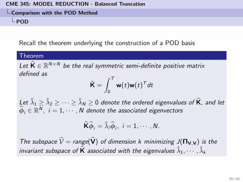
Recall the theorem underlying the construction of a POD basis

Theorem

Let K ∈ RN×N be the real symmetric semi-definite positive matrixdefined as

K =

∫ T0

w(t)w(t)Tdt

Let λ1 ≥ λ2 ≥ · · · ≥ λN ≥ 0 denote the ordered eigenvalues of K, and letφi ∈ RN , i = 1, · · · ,N denote the associated eigenvectors

Kφi = λi φi , i = 1, · · · ,N.

The subspace V = range(V) of dimension k minimizing J(ΠV,V) is the

invariant subspace of K associated with the eigenvalues λ1, · · · , λk

34 / 42


Comparison with the POD Method

POD for an Impulse Response

The response of an LTI system to a single impulse input with a zeroinitial condition is

w(t) = eAtB

Consequently, the reachability Gramian is

K =

∫ T0

w(t)w(t)Tdt =

∫ T0

eAtBBT eAT tdt = P

Unlike the Balanced Truncation method, the POD method does nottake into account the observability Gramian to determine the ROM,and therefore every observable state may be truncated

35 / 42


Application

CD Player System

The goal is to model the position of the lens controlled by a swingarm

2-inputs/2-outputs system

36 / 42


Application

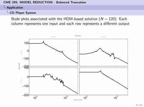
CD Player System

Bode plots associated with the HDM-based solution (N = 120): Eachcolumn represents one input and each row represents a different output

−200

−100

0

100

From: In(1)

To: O

ut(

1)

100

105

−200

−100

0

100

To: O

ut(

2)

From: In(2)

100

105

Bode Diagram

Frequency (rad/sec)

Magnitude (

dB

)

37 / 42


Application

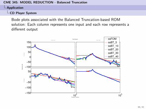
CD Player System

Bode plots associated with the Balanced Truncation-based ROMsolution: Each column represents one input and each row represents adifferent output

−100

−50

0

50

100

150From: In(1)

To: O

ut(

1)

105

−150

−100

−50

0

50

To: O

ut(

2)

From: In(2)

105

Bode Diagram

Frequency (rad/sec)

Magnitude (

dB

)

ssFOM

ssBT_5

ssBT_10

ssBT_20

ssBT_30

ssBT_40

38 / 42


Balanced POD Method

The Balanced POD Method

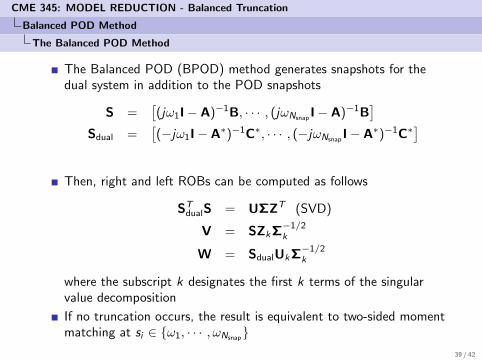
The Balanced POD (BPOD) method generates snapshots for thedual system in addition to the POD snapshots

S =[(jω1I− A)−1B, · · · , (jωNsnap I− A)−1B

]Sdual =

[(−jω1I− A∗)−1C∗, · · · , (−jωNsnap I− A∗)−1C∗

]Then, right and left ROBs can be computed as follows

STdualS = UΣZT (SVD)

V = SZkΣ−1/2k

W = SdualUkΣ−1/2k

where the subscript k designates the first k terms of the singularvalue decomposition

If no truncation occurs, the result is equivalent to two-sided momentmatching at si ∈ {ω1, · · · , ωNsnap}

39 / 42


Balanced POD Method

Balanced Truncation and POD in the Time Domain

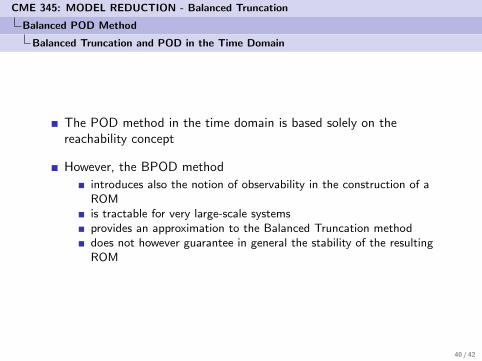
The POD method in the time domain is based solely on thereachability concept

However, the BPOD method

introduces also the notion of observability in the construction of aROMis tractable for very large-scale systemsprovides an approximation to the Balanced Truncation methoddoes not however guarantee in general the stability of the resultingROM

40 / 42


Balanced POD Method

Application

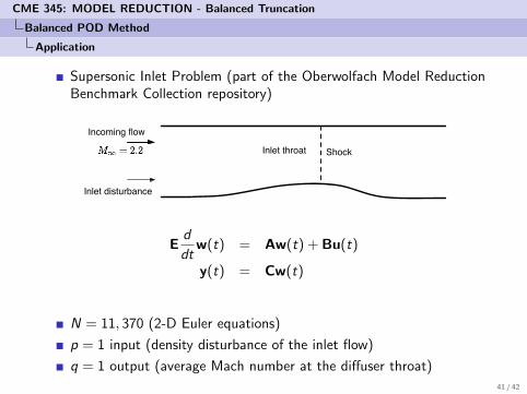
Supersonic Inlet Problem (part of the Oberwolfach Model ReductionBenchmark Collection repository)

Shock

Incoming flow

Inlet disturbance

Inlet throat

Ed

dtw(t) = Aw(t) + Bu(t)

y(t) = Cw(t)

N = 11, 370 (2-D Euler equations)

p = 1 input (density disturbance of the inlet flow)

q = 1 output (average Mach number at the diffuser throat)

41 / 42


Balanced POD Method

Application

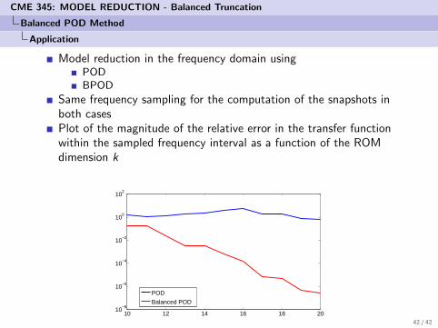
Model reduction in the frequency domain usingPODBPOD

Same frequency sampling for the computation of the snapshots inboth casesPlot of the magnitude of the relative error in the transfer functionwithin the sampled frequency interval as a function of the ROMdimension k

10 12 14 16 18 2010

−8

10−6

10−4

10−2

100

102

POD

Balanced POD

42 / 42

Documents

CME 345: MODEL REDUCTION - web.stanford.edu€¦ · CME 345: MODEL REDUCTION - Balanced Truncation Reachability and Observability Systems Considered Consider the following stable