Embed Size (px)
Citation preview
Coastal Inundation Mapping for Tasmania - Stage 2
Version 1
For the Department of Premier and Cabinet
26th September 2012
Dr Michael Lacey1, Dr John Hunter2 and Dr Richard Mount1
1 Blue Wren Group, School of Geography and Environmental Studies, University of Tasmania 2 Antarctic Climate and Ecosystems Cooperative Research Centre, University of Tasmania
Blue Wren Group, SGES, UTAS
Coastal Inundation Mapping Stage 2 V1 26/09/2012 Page 2 of 38
Citation
M.J. Lacey, J.R. Hunter and R.E. Mount (2012) Coastal Inundation Mapping for Tasmania - Stage 2. Report to the
Department of Premier and Cabinet by the Blue Wren Group, School of Geography and Environmental Studies,
University of Tasmania and the Antarctic Climate and Ecosystems Cooperative Research Centre
Blue Wren Group
Purpose: “To drive continuous improvement in the provision of
high quality environmental data and information that is
understandable and directly relevant to management
purposes.”
Acknowledgements
Special thanks go to Kathy McInnes, CSIRO for contributing the storm tide modelling for Tasmania.
Thanks also to
- Alice Palmer and Caroline Burbury, Research Office Commercialisation Unit, UTAS - Tessa Jakszewicz, ACE CRC,UTAS - James Chittleborough, NTC, BoM - ESRI Australia for assistance with ArcGIS software

Blue Wren Group, SGES, UTAS
Coastal Inundation Mapping Stage 2 V1 26/09/2012 Page 3 of 38
Summary
This report was prepared for the project “Coastal Inundation Stage 2” for the Tasmanian
Department of Premier and Cabinet and accompanies a set of GIS datasets produced in that
project. The project was concerned with mapping of a set of sea level rise scenarios around the
Tasmanian coast. This report is of a technical nature and is primarily intended to document the
methods used in the project. The sea level rise allowances used in this project have been supplied
by the Tasmanian Government to create coastal inundation area maps to support the development
of a coastal policy, and a coastal inundation planning code. The sea level rise allowances were
based on a regional sea-level projections and the A1FI emission scenario.
Outputs include:
a) A polygon shapefile map showing extents of expected permanent inundation associated
with 0.2, 0.4 and 0.8 metre sea level rise (coinciding with sea level rise scenarios above
2010 levels for years 2050, 2075 and 2100). These are mapped using the best available
digital elevation model (DEM), this being the Climate Futures LiDAR DEM or the
Tasmanian 25 metre DEM.
b) Maps of the inundation extents associated with a specified range of Annual Exceedance
Probabilities (AEP)s of 0.005%, 0.05%, 0.5%, 1%, 2% and 5 % for each of years 2010,
2050, 2075 and 2100, with one polygon dataset per specified year. These are mapped
using the best available DEM, this being the Climate Futures LiDAR DEM or the
Tasmanian 25 metre DEM.
c) An updated version of the Tasmanian height references layer, produced in part C of the
stage one project with inclusion of sea level rise heights in 0.1 metre increments to 1.2
metre at the 50% confidence level and the AEP heights specified in (b).
d) Documentation of methods, an example maps for communication purposes and metadata
on the datasets.

Blue Wren Group, SGES, UTAS
Coastal Inundation Mapping Stage 2 V1 26/09/2012 Page 4 of 38
Table of Contents Citation 2
Blue Wren Group 2
Acknowledgements 2
SUMMARY 3
TABLE OF CONTENTS 4
DEFINITIONS 5
INTRODUCTION 6
PROJECT AIM AND PURPOSE 6
INPUT DATASETS 7
LiDAR DEM 7
Tasmanian 25m DEM 8
Tidal range data 8
Storm Tide AEP data 9
Tasmanian Sea-Level Rise Allowances 9
MAPPING OF HIGH TIDES AND SLR 10
Geoprocessing implementation – “High Tides and SLR” 10 SLR polygon generation and processing for non-LiDAR areas ............................................................................. 11 Dataset combination ........................................................................................................................................... 11
Output Dataset – “High Tides and SLR” 11
Discussion – “High Tides and SLR” 12
STORM TIDE EVENT PLUS SLR 13
Geoprocessing implementation – “Storm Tide Event plus SLR” 13
Output Datasets – “Storm Tide Annual Exceedance probabilities” 14
Discussion – “Storm Tide Event plus SLR” 16
COASTAL INUNDATION HEIGHT REFERENCE DATASET 17
Output Dataset – Coastal Inundation Height Reference 19
Discussion – Coastal Inundation Height Reference 20
REFERENCES 21
APPENDIX 1. DRAFT METADATA 22
Coastal High Water plus Sea Level Rise Inundation Modelling metadata – Tasmania, Version 2 22
Storm Tide plus Sea Level Rise Inundation Modelling metadata – Tasmania, Version 2 26
Coastal Inundation Height Reference metadata – Tasmania, Version 3.2 30
APPENDIX 2. CSIRO STORM TIDE MODELLING 34

Blue Wren Group, SGES, UTAS
Coastal Inundation Mapping Stage 2 V1 26/09/2012 Page 5 of 38
Definitions
A1FI The IPCC’s “high emission” scenario
ACE CRC Antarctic Climate & Ecosystems Cooperative Research Centre
AEP Annual Exceedance Probability
AHD Australian Height Datum is the current official standard Australian height
reference (ICSM, 2006). For Tasmania it is based on mean sea level at Burnie
and Hobart tide gauges in 1972. For a number of reasons including suboptimal
location of some tide gauges, limited period of the reference sea level
determination and non-inclusion of sea level topography AHD is an
approximation of mean sea level only.
CSIRO Commonwealth Scientific and Industrial Research Organisation
DEM Digital elevation model, a surface representing the surface heights of the land
DPaC Department of Premier and Cabinet
GIS Geographic Information System
IPCC Intergovernmental Panel on Climate Change
ISHW Indian springs high water. Defined as Mean Sea Level plus the amplitudes of
the tidal constituents: M2 + S2 + O1 + K1.
ISLW Indian springs low water. Defined as Mean Sea Level minus the amplitudes of
the tidal constituents: M2 + S2 + O1 + K1.
LiDAR Light detection and ranging (like “radar”, or radio detection and ranging, but
using laser light pulses instead of radio pulses)
MHW The average of all high waters over a period of time (ICSM, 2007). For
inundation modelling, the high water used was the “NTC High Water” (see
below).
MSL Mean Sea Level For a tidal station Mean Sea Level is the mean over a period of
time of the hourly heights at that station (ICSM, 2007).
NTC National Tidal Centre, Bureau of Meteorology
NTC High Water The standard tidal range grid modelled by the National Tidal Centre (NTC)
used to model the approximate high water mark, which in most cases also
represents the historically mapped coastline well. The NTC tidal range is the
height in metres between Mean Sea Level and Indian Spring Low Water
multiplied by two to give an estimate of the complete tidal range. It is twice the
sum of the amplitudes of the four main tidal constituents, M2, S2, O1 and K1.
For Part a) inundation modelling, the high water used was the NTC modelled
high water, which is at a height of half the NTC tide range above Mean Sea
Level.
SLR Sea level rise
Storm Tide A combination of the tidal component plus any raised sea level due to wind set
up or reduced air pressure. It is what is measured at tide gauges during a storm
event.
UTAS University of Tasmania

Blue Wren Group, SGES, UTAS
Coastal Inundation Mapping Stage 2 V1 26/09/2012 Page 6 of 38
Introduction This report was prepared for the project “Coastal Inundation Stage 2” for the Tasmanian
Department of Premier and Cabinet (DPaC) and accompanies a set of GIS datasets produced in
that project. The project was concerned with mapping of a set of sea level rise scenarios around
the Tasmanian coast. This report is of a technical nature and is primarily intended to document
the methods used in the project. The sea level rise allowances used in this project have been
supplied by the Tasmanian Government to create coastal inundation area maps to support the
development of a coastal policy, and a coastal inundation planning code. The sea level rise
allowances were based on regional sea-level projections and the A1FI emission scenario.
Project aim and purpose This project follows on from the coastal inundation stage one project, also known as the
Tasmanian Coastal Inundation Mapping Project, Mount et al. (2010) and Mount et al. (2011)
which consisted of the following components:
Part A. Mapping of locations potentially affected by sea level rise at 0.2 metre increments up to
1.2 metre plus 1.6 and 2.0 metre above a base tidal height.
Part B. Mapping of locations potentially affected by flooding associated with storm-tide
exceedance events at exceedance probabilities of 25%, 50% and 75% averaged for the
periods 2010-2050 and 2010-2100, with and without sea level rise.
Part C. Provided coastal reference heights in a 1 kilometre grid covering the entire Tasmanian
coastline. This presented the height data from parts A and B and instead of mapping the
heights onto the ground it could be used as a “look up” or “reference” map to identify key
hazard threshold heights within specific (1 km square) areas. Reference sea level rise
inundation heights were in most regions based on the modelled NTC tidal heights and were
calculated at 5%, 50% and 95% confidence levels based on error estimates. Storm tide
calculations were provided for LiDAR areas only.
The purpose of the current project was to conduct additional mapping of tidal inundation in areas
not covered by the Climate Futures LiDAR DEM and to map storm tide as annual exceedance
probabilities (AEPs) for specified years (2010, 2050, 2075 and 2100).
Specified components for the current project were:
- To provide a polygon shapefile map showing extents of expected permanent inundation
associated with 0.2, 0.4 and 0.8 metre sea level rise (coinciding with sea level rise
scenarios above 2010 levels for years 2050, 2075 and 2100). These were to be mapped
using the best available DEM, this being the Climate Futures LiDAR DEM or the
Tasmanian 25 metre DEM.
- To map the inundation extents associated a specified range of AEPs (0.005%, 0.05%,
0.5%, 1%, 2% and 5 %) for each of years 2010, 2050, 2075 and 2100, with one polygon
shapefile per specified year. These were to be mapped using the best available DEM, this
being the Climate Futures LiDAR DEM or the Tasmanian 25 metre DEM.
- Add to the Tasmanian height references layer, produced in part C of the stage one project,
sea level rise heights in 0.1 metre increments to 1.2 metre at the 50% confidence level and
the AEP heights specified in (b).
- Provide documentation of methods, an example map for communication purposes and
metadata on the datasets.

Blue Wren Group, SGES, UTAS
Coastal Inundation Mapping Stage 2 V1 26/09/2012 Page 7 of 38
Input Datasets Following is a brief description of the input datasets used in the mapping. A number of issues are
highlighted and the approaches taken to address those issues are presented.
LiDAR DEM The Climate Futures LiDAR dataset as supplied via the Information & Land Services Division
(ILS) of the Department of Primary Industries, Parks, Water and Environment (DPIPWE). The
dataset was collected by Digital Mapping Australia (DiMAP) for the Antarctic Climate &
Ecosystems Cooperative Research Centre (ACE CRC) under the Climate Futures for Tasmania
project. DEM tiles are 1 km x 1 km in size with 50 metre fringe, giving a 100 m overlap of tiles.
The individual grid cells are 1 m x 1 m and have stated horizontal and vertical accuracies of +/-
25 cm.
Preliminary assessment of the LiDAR dataset has revealed a number of limitations which
constrained the reliability of the dataset for use in inundation mapping. The principal limitation
was height discrepancies in a number of areas particularly where there were no nearby survey
control points. Affected areas included large parts of Port Sorell, Pittwater and the Tasman
Peninsula. Inundation mapping using the LiDAR DEM in these areas resulted in significant over
or under estimation of inundation heights. In these areas the Tasmanian 25 metre DEM was
substituted as the elevation reference. Figure 1 shows the extent of the Climate Futures LiDAR
DEM. Areas considered unreliable (blue) were excluded from the inundation mapping.
There is some reason to believe that heights of some individual survey control points used in
production of the LiDAR DEM were incorrect or the registered position was displaced from their
correct position in relation to the LiDAR. Examples of this include wetlands in part of the upper
Derwent and in the region of Knights Road, Connellys Marsh.
Thick vegetation that obscures the ground surface can also produce false LiDAR heights with an
upward bias from the true ground surface. The height difference produced may be small but has
the potential to be sufficient to have an effect on inundation modelling outcomes in some areas.
Figure 1. Extent of the Climate Futures LiDAR DEM showing areas considered reliable (red) and unreliable (blue)
for inundation mapping. The unreliable areas were excluded from the inundation mapping.

Blue Wren Group, SGES, UTAS
Coastal Inundation Mapping Stage 2 V1 26/09/2012 Page 8 of 38
Tasmanian 25m DEM
The Tasmanian 2nd
Edition 25 metre DEM (Information & Land Services Division, DPIPWE)
was used to fill in areas not covered by the LiDAR DEM or where the LiDAR DEM was
considered unreliable. The 25 metre DEM has a floating point dataset and has been produced
from 1:25,000 Series maps, primarily by interpolation between 10 metre contours. This
interpolation method lends itself to errors in areas where contours are widely spaced such as low
lying coastal areas. However this DEM is currently the best available alternative to the LiDAR
DEM over coastal areas and can at least provide an indication of areas potentially subject to
inundation due to sea level rise.
Tidal range data
Over the majority of the mapped area, the standard National Tidal Centre (NTC) modelled tidal
range grid was used to determine the approximate high water mark. This was supplemented by
additional published tidal height data for the Tamar Valley and Macquarie Harbour (Mount et al
2011).
The NTC tidal range data which is accessible via the Bureau of Meteorology (BOM) web site
(www.bom.gov.au/oceanography/tides/index_range.shtml) was obtained from the National Tidal
Centre in the form of a five minute resolution grid of points including coverage of Tasmanian
coastal waters (ftp.bom.gov.au/anon/home/ntc/james/model/range_m_aus5min.zip).
The NTC tidal range is the height in metres between Mean Sea Level and Indian Spring Low
Water multiplied by two to give an estimate of the complete tidal range. It includes the four main
tidal constituents, M2, S2, O1 and K1, and was calculated as:
Tidal range = (M2 + S2 + O1 + K1) amplitude * 2
For inundation mapping purposes it was assumed that the midpoint in the NTC tidal range
represents mean sea level (MSL) and that this height is also at zero metres AHD. Regional
variations in tidal dynamics may mean that the midpoint in the range is not always MSL. Also
MSL, although intended as the base datum of AHD, is only approximate due to errors in methods
used to derive AHD. Sea level rise in the time since AHD was derived has also added an amount
to MSL which will vary by region.
For the purposes of the current mapping, half the NTC tidal range was considered to represent an
approximation of the difference between MSL and high tidal height, and when added to MSL the
total height should approximate, though tend to be higher than, the height of the mapped coastal
high water mark. In this report this height is referred to as “NTC High Water”.
The Average Recurrence Interval (ARI; same as return period) for Burnie, George Town and
Hobart for both tidal predictions (i.e. tide only) and observations (tide + surge) for a level equal
to "Indian Springs High Water" (ISHW, defined as Mean Sea Level plus the amplitudes of the
tidal constituents: M2 + S2 + O1 + K1) were extracted and are presented in Table 1 below. The
results are based on periods of approximately 30 years.
There is a lot of variation in the ARI, even around Tasmania and the inclusion of surges (i.e.
within the observational data) has a significant effect. The main difference between the north
(Burnie and George Town) and the south (Hobart) is that the main semidiurnal tide is much larger
in the north, which reduces the influence of the other tidal constituents (including those not
contributing to ISHW). Therefore, in the north, the ISHW is a better measure of the maximum
possible tide whereas in the south, all the other constituents (not included in the definition of
ISHW) make the highest tide significantly larger than ISHW. In the north, therefore, ISHW is
exceeded much less often than in the south.
Blue Wren Group, SGES, UTAS
Coastal Inundation Mapping Stage 2 V1 26/09/2012 Page 9 of 38
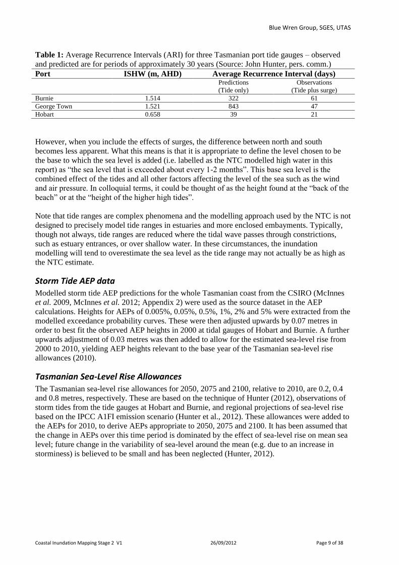
Table 1: Average Recurrence Intervals (ARI) for three Tasmanian port tide gauges – observed
and predicted are for periods of approximately 30 years (Source: John Hunter, pers. comm.)
Port ISHW (m, AHD) Average Recurrence Interval (days) Predictions
(Tide only)
Observations
(Tide plus surge)
Burnie 1.514 322 61
George Town 1.521 843 47
Hobart 0.658 39 21
However, when you include the effects of surges, the difference between north and south
becomes less apparent. What this means is that it is appropriate to define the level chosen to be
the base to which the sea level is added (i.e. labelled as the NTC modelled high water in this
report) as “the sea level that is exceeded about every 1-2 months”. This base sea level is the
combined effect of the tides and all other factors affecting the level of the sea such as the wind
and air pressure. In colloquial terms, it could be thought of as the height found at the “back of the
beach” or at the “height of the higher high tides”.
Note that tide ranges are complex phenomena and the modelling approach used by the NTC is not
designed to precisely model tide ranges in estuaries and more enclosed embayments. Typically,
though not always, tide ranges are reduced where the tidal wave passes through constrictions,
such as estuary entrances, or over shallow water. In these circumstances, the inundation
modelling will tend to overestimate the sea level as the tide range may not actually be as high as
the NTC estimate.
Storm Tide AEP data Modelled storm tide AEP predictions for the whole Tasmanian coast from the CSIRO (McInnes
et al. 2009, McInnes et al. 2012; Appendix 2) were used as the source dataset in the AEP
calculations. Heights for AEPs of 0.005%, 0.05%, 0.5%, 1%, 2% and 5% were extracted from the
modelled exceedance probability curves. These were then adjusted upwards by 0.07 metres in
order to best fit the observed AEP heights in 2000 at tidal gauges of Hobart and Burnie. A further
upwards adjustment of 0.03 metres was then added to allow for the estimated sea-level rise from
2000 to 2010, yielding AEP heights relevant to the base year of the Tasmanian sea-level rise
allowances (2010).
Tasmanian Sea-Level Rise Allowances
The Tasmanian sea-level rise allowances for 2050, 2075 and 2100, relative to 2010, are 0.2, 0.4
and 0.8 metres, respectively. These are based on the technique of Hunter (2012), observations of
storm tides from the tide gauges at Hobart and Burnie, and regional projections of sea-level rise
based on the IPCC A1FI emission scenario (Hunter et al., 2012). These allowances were added to
the AEPs for 2010, to derive AEPs appropriate to 2050, 2075 and 2100. It has been assumed that
the change in AEPs over this time period is dominated by the effect of sea-level rise on mean sea
level; future change in the variability of sea-level around the mean (e.g. due to an increase in
storminess) is believed to be small and has been neglected (Hunter, 2012).

Blue Wren Group, SGES, UTAS
Coastal Inundation Mapping Stage 2 V1 26/09/2012 Page 10 of 38
Mapping of High Tides and SLR The “High Tides and SLR” component of this mapping, used the “bathtub” inundation method
(Eastman, 1993). The “bathtub” or “still water” method is essentially a simplified representation
of reality generated with electronic mapping systems (GIS). The method assumes a calm still sea
surface. The sea level components (including sea level rise levels and the tidal range) were
combined with a digital elevation model (DEM) to calculate a spatial grid over the area of interest
showing the locations likely to be inundated given the model settings and constraints. The
positions of possible future, or “indicative”, shorelines were extracted from the grid model. Given
that the mapped coastline is usually at the high water mark and that most human activities are
landwards of the high water mark, this was considered a useful base height to which to add the
sea level rise estimates. The resultant “indicative” shorelines can be considered as new positions
for the “back of the beach” in the simple virtual reality of the model.
The previous mapping presented in Mount et al. (2011) followed a probability based approach in
which error probability levels were also calculated based on the error probabilities propagated
from the input datasets. This approach produced output datasets representing 5%, 50% and 95%
likelihoods that a new shore position was at or above the mapped height based on error inputs.
Algorithms used in this mapping approach have been documented in Mount et al. (2011). The
current mapping is required at the 50% probability level only, meaning that a much simpler
additive mapping approach could be applied. Consequently reference to the 50% probability level
has been omitted and is assumed.
Inputs to this mapping can be summarised as follows:
- The Climate Futures LiDAR DEM or where that was not available the Tasmanian 25 metre
DEM was substituted,
- The Mean Sea Level (MSL) is assumed to equal 0 m Australian Height Datum (AHD),
- Tide estimates (in metres AHD), based on the NTC High Water Mark (see Definitions
section) for the majority of the mapped area or published tidal data for Tamar River and
Macquarie Harbour, and
- A series of sea level rise heights, these being 0.2, 0.4 and 0.8 metres.
The primary outputs were a series polygon datasets representing the most likely position of the
shoreline with 0.2, 0.4 or 0.8 metre sea level rise allowance relative to 2010. Datasets were
combined into a single polygon shapefile.
Geoprocessing implementation – “High Tides and SLR” Existing SLR polygon datasets produced in the stage one project (Table 2) were used as the data
inputs for the LiDAR areas. Methods that were used to produce these datasets are documented in
Mount et al. (2011). New mapping was required for parts of the coast not covered by the Climate
Futures LiDAR DEM. In those regions mapping was based on the Tasmanian 25 metre DEM as
detailed below. For the 25 metre DEM areas the combined tidal inundation and sea level rise was
rounded-up to the nearest whole metre. Mapped outputs for LiDAR and non-LiDAR areas were
then combined into the final dataset. Geoprocessing was conducted using ArcGIS 10.0.

Blue Wren Group, SGES, UTAS
Coastal Inundation Mapping Stage 2 V1 26/09/2012 Page 11 of 38
Table 2: Datasets used from the stage one project
Dataset from stage one project Description NTC_TR_20SLR_50pct.shp Polygon mapping of expected tidal inundation with 20, 40 and
80 cm sea level rise in LiDAR areas excluding southern
Tamar. NTC_TR_40SLR_50pct.shp
NTC_TR_80SLR_50pct.shp
TamarSouth_MHW_20SLR_50pct.shp Polygon mapping of expected tidal inundation with 20, 40 and
80 cm sea level rise in the southern part of the Tamar Valley,
east of MGA 50200 metres. TamarSouth_MHW_40SLR_50pct.shp
TamarSouth_MHW_80SLR_50pct.shp
SLR polygon generation and processing for non-LiDAR areas
Modelled tidal range data was available as points around the whole Tasmanian coast. The
modelled points were all on the seaward side of the coastline and usually did not extend to the
coast, especially in the vicinity of bays and estuaries. A spline interpolation with barriers was
used to create the tidal range surface extending across the land. In Macquarie Harbour the tidal
height as published by Koehnken L. (1996) was used.
Sea level rise increments to the specified heights were added to the tidal heights. For the 25 metre
DEM areas only, the combined tidal inundation and sea level rise was then rounded-up to the
nearest whole metre. Tidal surfaces with SLR were subtracted from the 25m DEM and cells of
the resultant surface with a value less than zero were designated as inundated. Outputs were
converted to polygon shapefiles which showed areas expected to be inundated under the modelled
scenarios. The polygon shapefiles were clipped to a polygon version of the coastline.
Dataset combination
LiDAR based and non-LiDAR based datasets were combined into a single state-wide dataset.
A polygon mask, identifying location of reliable LiDAR areas, was used to clip out those areas
from the LiDAR based polygon outputs and to erase the same areas from the 25 metre DEM
based outputs. LiDAR and 25 m DEM based datasets were then merged to produce the combined
shapefile.
Output Dataset – “High Tides and SLR”
The output is a single combined polygon dataset representing the areas of permanent (tidal)
inundation that can be expected for the years 2050, 2075 and 2100. Concentric polygon areas
represent regions expected to be inundated by sea level rise of 0.2, 0.4 and 0.8 metre respectively
above 2010 levels. The Climate Futures LiDAR DEM has been used as the height reference
where it was available and considered to be reliable. The Tasmanian 25 metre DEM was used in
all other areas. The sea level reference was the NTC modelled high water except is the Tamar
Valley and Macquarie Harbour where alternative published mean high tide heights were used.
The output dataset name is “TidalInundationModel_V2” and is provided in file geodatabase
(.gdb) format with the dataset having the same name as the geodatabase in which it is enclosed.
The dataset is projected in GDA 94 MGA Zone 55. Attributes are listed in Table 3. Attribution
has been included to allow selection of inundation polygons associated with each of the target
years and also to distinguish between polygons that are contiguous or non-contiguous with the
coast. Table 4 list queries in ArcGIS that can be used to select contiguous or non-contiguous
inundation polygon extents.

Blue Wren Group, SGES, UTAS
Coastal Inundation Mapping Stage 2 V1 26/09/2012 Page 12 of 38
Table 3: Attribute fields for TidalInundationModel_V2.shp
Field Name Data type Details TR2050 Text “0.2 m” indicates projected inundation level in 2050.
TR2075 Text “0.4 m” indicates projected inundation level in 2075.
TR2100 Text “0.8 m” indicates projected inundation level in 2100.
IC2050 Integer (1 = contiguous with coast; 0 = not contiguous with coast) at 0.2 m inundation.
IC2075 Integer (1 = contiguous with coast; 0 = not contiguous with coast) at 0.4 m inundation.
IC2100 Integer (1 = contiguous with coast; 0 = not contiguous with coast) at 0.8 m inundation.
SL_Ref Text NTC_HW (= NTC modelled high water)
NTC_HW Extr (= NTC modelled high water extrapolated in Tamar and on
southern side of Robbins Island)
MHT (= Mean high tide in Launceston area)
MHT Mac Hb (= mean high tide Macquarie Harbour)
SLR Text Sea level rise level (in metres) in which the polygon appears “inundated”.
DEM_Ref Text CFL (= Climate Futures LiDAR)
DEM25 (= State 25 m DEM)
Note: Inundation heights in the 25 m DEM areas have been rounded up to
the nearest whole metre.
Shape_Length Floating point Polygon perimeter in metres.
Shape_Area Floating point Polygon area in square metres.
Table 4: ArcGIS queries for selection of inundation extents that are contiguous or not
contiguous with the coast from the tidal inundation dataset
To select Query Polygons contiguous with the coast that are expected to be inundated in 2050. "TR2050" = '0.2 m' AND "IC2050" = 1
Polygons not contiguous but potentially inundation in 2050 under some
circumstances.
"TR2050" = '0.2 m' AND "IC2050" = 0
Polygons contiguous with the coast that are expected to be inundated in 2075. "TR2075" = '0.4 m' AND "IC2075" = 1
Polygons not contiguous but potentially inundation in 2075 under some
circumstances.
"TR2075" = '0.4 m' AND "IC2075" = 0
Polygons contiguous with the coast that are expected to be inundated in 2100. "TR2100" = '0.8 m' AND "IC2100" = 1
Polygons not contiguous but potentially inundation in 2100 under some
circumstances.
"TR2100" = '0.8 m' AND "IC2100" = 0
Discussion – “High Tides and SLR”
It should be noted that not all variables relevant to the accurate modelling and prediction of new
shoreline positions are currently available for all the locations of interest around the coast, that is,
there are limitations on the available data inputs at the Tasmanian scale. For example,
- The high resolution Climate Futures LiDAR DEM currently only covers about a third of the
more highly populated coastlines and is known to have inaccurate heights in some areas.
- The lower resolution 25 metre DEM may give an indication only of potential coastline
positions with sea level rise.
- The tide range data for Tasmania is limited to either direct observations at the main tide
gauges or, for other locations along the shore, to modelled estimates from the National Tidal
Centre, Bureau of Meteorology. The tides in more enclosed bays and estuaries or around
islands can be substantially different to those shown in the available data.
- Also, there is no consideration of the complex interactions between erosion, coastal recession
and inundation. The “bathtub” or “still water” method is essentially a passive model and
assumes a calm sea surface. It is useful because it is a simple, fast method that indicates
locations with the potential for inundation and can, if used judiciously and with other lines of
evidence, assist with prioritising further activity.

Blue Wren Group, SGES, UTAS
Coastal Inundation Mapping Stage 2 V1 26/09/2012 Page 13 of 38
Storm Tide Event plus SLR In the absence of sea-level rise, future flooding events from the sea depend on the tides, storm
surges and waves. While the tides are predictable, future storm surges and waves may only be
described in a statistical sense. For example, the time and height of high water at a given location
is known at any future time from our knowledge of past tides and of the motions of the Sun and
the Moon. However, future storm surges are generally quantified by the average time between
events when a certain level is exceeded (the "return period" or "average recurrence interval"), or
by the probability that a certain level is exceeded once or more during a given period (e.g. the
"Annual exceedance probability" or AEP). Similar statistics may be applied to the occurrence of
waves, although the effects of waves are not specifically included in the projections provided
here. For the present work, tides and storm surges ("storm tides") around the Tasmanian coastline
were derived from numerical modelling by Kathleen McInnes of CSIRO (see Appendix 2). From
these results were derived heights for AEPs of 0.005%, 0.05%, 0.5%, 1%, 2% and 5%. As
described in the Section “Storm Tide AEP Data”, the modelled AEP heights were adjusted to best
fit observations from Hobart and Burnie, and to relate to the year 2010, the base year for the
Tasmanian sea-level rise allowances.
Under climate change, flooding events from the sea will become more frequent, mainly due to the
effect of sea-level rise. Future sea level has been estimated by numerous modelling groups around
the world and is regularly collated and summarised by the Intergovernmental Panel on Climate
Change (IPCC) in their Assessment Reports. These estimates are, however, accompanied by
significant uncertainty (both due to uncertainty in the science and uncertainty in future emissions
of greenhouse gases). The sea-level rise allowances used in this project have been supplied by the
Tasmanian Government to create coastal inundation area maps to support the development of a
coastal policy, and a coastal inundation planning code. These allowances are based on the
technique of Hunter (2012), observations of storm tides from the tide gauges at Hobart and
Burnie, and regional projections of sea-level rise based on the IPCC A1FI emission scenario
(Hunter et al., 2012).
The Tasmanian sea-level rise allowances (0.2, 0.4 and 0.8 metres for 2050, 2075 and 2100,
relative to 2010, respectively) were then added to the modelled heights for 2010 for AEPs of
0.005%, 0.05%, 0.5%, 1%, 2% and 5%, to yield the 24 data sets of heights used for the
inundation mapping.
Geoprocessing implementation – “Storm Tide Event plus SLR”
Twenty four “Storm Tide plus SLR” height datasets representing the heights for each of the 6
AEPs (0.005%, 0.05%, 0.5%, 1%, 2% and 5%) and each of the four years (2010, 2050, 2075 and
2100) were geographically mapped. Each of the 24 AEP height datasets represented calculated
storm tide plus sea level rise exceedance heights for sea level rise scenarios as specified by the
Tasmanian Government to create coastal inundation area maps to support the development of a
coastal policy, and a coastal inundation planning code.
GIS processing was conducted using ArcGIS 10.0 with the majority of processing being scripted
using Python 2.6.5. The main geoprocessing steps are summarised as follows.
A spline with barriers interpolation method was used to calculate a series of height surfaces, from
a set of AEP datasets for the year 2000. Sea level rise heights of 0.03, 0.23, 0.43 and 0.83 metre
were added to the height surfaces to calculate AEP height surfaces for the years 2010, 2050, 2075
and 2100 respectively. LiDAR areas were processed as sixteen mosaicked regions and the 25

Blue Wren Group, SGES, UTAS
Coastal Inundation Mapping Stage 2 V1 26/09/2012 Page 14 of 38
metre DEM was processed as a single state-wide region. For the 25 metre DEM areas only, the
combined AEP inundation and sea level rise was rounded-up to the nearest whole metre. AEP
height surfaces were subtracted from the LiDAR and 25m DEM surfaces and cells of the resultant
surface with a value less than zero were designated as inundated. Outputs were converted to
polygon shapefiles which showed areas expected to be inundated under the modelled scenarios.
This polygonisation step used the “no_simplify” option. The polygon layers were then clipped to
a polygon version of the coastline. For each target year a union step was used to combine the
AEP level polygon datasets into single polygon dataset for each region. A series of erase steps
were then used to remove overlapping areas before merging the sixteen LiDAR mapped regions
into a combined shapefile for each target year. A polygon mask, identifying location of reliable
LiDAR areas, was used to clip out those areas from the LiDAR based polygon outputs and to
erase the same areas from the 25 metre DEM based outputs. LiDAR and 25 m DEM datasets
were then merged to produce combined state-wide polygon shapefiles for each target year.
Datasets were converted to geodatabase format to reduce file size and to speed up screen refresh
times.
Output Datasets – “Storm Tide Annual Exceedance probabilities” AEP datasets are listed in Table 5 and are provided in file geodatabase format with the dataset
having the same name as the geodatabase in which it is enclosed. All of the datasets are projected
in GDA 94 MGA Zone 55. Attributes of the datasets are listed in Table 6. Figure 2 illustrates how
inundation extents are represented in each dataset as concentric polygons for each AEP level.
Table 5: Storm Tide AEP Datasets
Dataset Name File geodatabase Target
Year
Projected sea level
rise (m) StormTide_AEP_2010_V2 Storm_Tide_AEP_2010_V2.gdb 2010 0
StormTide_AEP_2050_V2 Storm_Tide_AEP_2050_V2.gdb 2050 0.2
StormTide_AEP_2075_V2 Storm_Tide_AEP_2075_V2.gdb 2075 0.4
StormTide_AEP_2100_V2 Storm_Tide_AEP_2100_V2.gdb 2100 0.8
Table 6: Attributes of the Storm Tide AEP Datasets
Field Name Data type Details AEP5pct Text “5%” indicates inundation at 5% AEP level.
AEP2pct Text “2%” indicates inundation at 2% AEP level.
AEP1pct Text “1%” indicates inundation at 1% AEP level.
AEP_5pct Text “0.5%” indicates inundation at 0.5% AEP level.
AEP_05pct Text “0.05%” indicates inundation at 0.05% AEP level.
AEP_005pct Text “0.005%” indicates inundation at 0.005% AEP level.
IC5pct Integer (1 = contiguous with coast; 0 = not contiguous with coast) at 5% AEP level.
IC2pct Integer (1 = contiguous with coast; 0 = not contiguous with coast) at 2% AEP level.
IC1pct Integer (1 = contiguous with coast; 0 = not contiguous with coast) at 1% AEP level.
IC_5pct Integer (1 = contiguous with coast; 0 = not contiguous with coast) at 0.5% AEP level.
IC_05pct Integer (1 = contiguous with coast; 0 = not contiguous with coast) at 0.05% AEP level.
IC_005pct Integer (1 = contiguous with coast; 0 = not contiguous with coast) at 0.005% AEP level.
AEP_Level Text First AEP level in which the polygon appears “inundated”.
SLR Text Sea level rise for target year (2010, 0.0 m; 2050, 0.2 m; 2075, 0.4 m; 2100, 0.8
m).
DEM_Ref Text CFL (= Climate Futures LiDAR)
DEM25 (= State 25 m DEM)
Note: Inundation heights in the 25 m DEM areas have been rounded up to
the nearest whole metre.
Shape_Length Floating point Polygon perimeter in metres.
Shape_Area Floating point Polygon area in square metres.

Blue Wren Group, SGES, UTAS
Coastal Inundation Mapping Stage 2 V1 26/09/2012 Page 15 of 38
Figure 2. Example of the AEP inundation polygon mapping, illustrating how inundation extents are represented in
each dataset as concentric polygons for each AEP level. Olive green lines on this map are roads, grey area is un-
inundated land and white is seaward of the coast.
Attribution has been included to allow selection of inundation polygons associated with each of
the target years and also to distinguish between polygons that are contiguous or non-contiguous
with the coast. Table 7 lists queries in ArcGIS that can be used to select contiguous or non-
contiguous inundation polygon extents for the AEP datasets.
Table 7: ArcGIS queries for selection of inundation extents that are contiguous or not
contiguous with the coast from the AEP datasets
To select Query Polygons contiguous with the coast that are expected to be inundated
at 5% AEP level.
"AEP5pct" = '5%' AND "IC5pct" = 1
Polygons not contiguous but potentially inundation at 5% AEP level
under some circumstances.
"AEP5pct" = '5%' AND "IC5pct" = 0
Polygons contiguous with the coast that are expected to be inundated
at 2% AEP level.
"AEP2pct" = '2%' AND "IC2pct" = 1
Polygons not contiguous but potentially inundation at 2% AEP level
under some circumstances.
"AEP2pct" = '2%' AND "IC2pct" = 0
Polygons contiguous with the coast that are expected to be inundated
at 1% AEP level.
"AEP1pct" = '1%' AND "IC1pct" = 1
Polygons not contiguous but potentially inundation at 1% AEP level
under some circumstances.
"AEP1pct" = '1%' AND "IC1pct" = 0
Polygons contiguous with the coast that are expected to be inundated
at 0.5% AEP level.
"AEP_5pct" = '0.5%' AND "IC_5pct" = 1
Polygons not contiguous but potentially inundation at 0. 5% AEP level
under some circumstances.
"AEP_5pct" = '0.5%' AND "IC_5pct" = 0
Polygons contiguous with the coast that are expected to be inundated
at 0.05% AEP level.
"AEP_05pct" = '0.05%' AND "IC_05pct" = 1
Polygons not contiguous but potentially inundation at 0.05% AEP
level under some circumstances.
"AEP_05pct" = '0.05%' AND "IC_05pct" = 0
Polygons contiguous with the coast that are expected to be inundated
at 0.005% AEP level.
"AEP_005pct" = '0.005%' AND "IC_005pct" = 1
Polygons not contiguous but potentially inundation at 0.005% AEP
level under some circumstances.
"AEP_005pct" = '0.005%' AND "IC_005pct" = 0

Blue Wren Group, SGES, UTAS
Coastal Inundation Mapping Stage 2 V1 26/09/2012 Page 16 of 38
Discussion – “Storm Tide Event plus SLR” The areas covered by the Storm Tide AEP polygon mapping show a range of AEP percentages.
Individual polygons have the attribute “AEP_Level” which specifies the mapped AEP percentage
to which the polygon relates. The precise landward extent (i.e. edge or boundary) of the polygon
represents the specified AEP for the prescribed year and the area within the remainder of the
polygon has a higher exceedance probability.
For example, for a polygon with “AEP_Level” of 0.05% in the dataset
StormTide_AEP_2100_V1_2:
- Anything lying at ground level at the landward edge (or boundary) of the polygon (“flood
plain”) has an AEP of 0.05% of being flooded by a storm tide once or more during 2100,
- Any land seaward of this line (i.e. lying inside this flooding zone) has a higher probability
of being flooded, and
- Any land landward of this line (i.e. lying outside this flooding zone) has a lower
probability of being flooded.
A number of caveats accompany these results:
- These storm-tide coastal flooding zones include the effects of tides, storm surges and sea-
level rise only. They do not include the effects of wave set-up or wave run-up. Additional
allowances (“freeboard”) may therefore need to be made for effects associated with
waves.
- The projections of sea-level rise used in these calculations involve considerable
uncertainty, arising from an imperfect understanding both of the science and of the
world's future emissions.
- These results relate to the increase in the probability of extreme events caused by a rise in
mean sea level; they do not make any projections of changes in storm tides.
Blue Wren Group, SGES, UTAS
Coastal Inundation Mapping Stage 2 V1 26/09/2012 Page 17 of 38
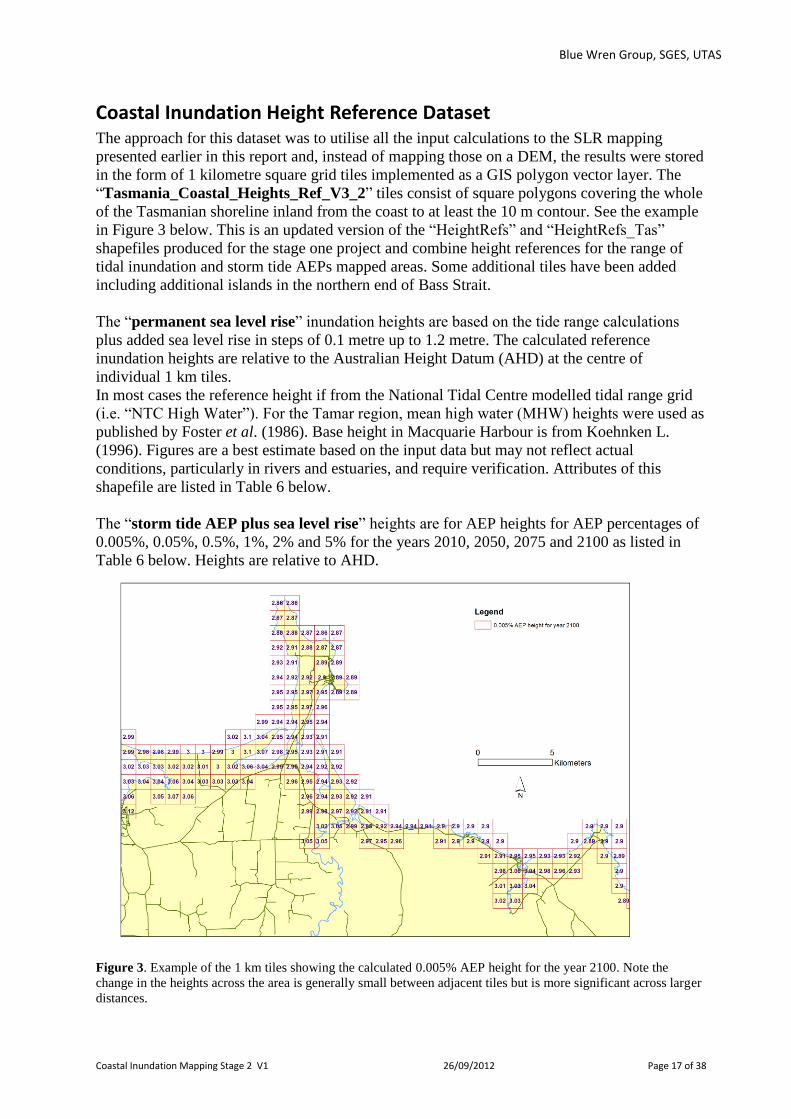
Coastal Inundation Height Reference Dataset The approach for this dataset was to utilise all the input calculations to the SLR mapping
presented earlier in this report and, instead of mapping those on a DEM, the results were stored
in the form of 1 kilometre square grid tiles implemented as a GIS polygon vector layer. The
“Tasmania_Coastal_Heights_Ref_V3_2” tiles consist of square polygons covering the whole
of the Tasmanian shoreline inland from the coast to at least the 10 m contour. See the example
in Figure 3 below. This is an updated version of the “HeightRefs” and “HeightRefs_Tas”
shapefiles produced for the stage one project and combine height references for the range of
tidal inundation and storm tide AEPs mapped areas. Some additional tiles have been added
including additional islands in the northern end of Bass Strait.
The “permanent sea level rise” inundation heights are based on the tide range calculations
plus added sea level rise in steps of 0.1 metre up to 1.2 metre. The calculated reference
inundation heights are relative to the Australian Height Datum (AHD) at the centre of
individual 1 km tiles.
In most cases the reference height if from the National Tidal Centre modelled tidal range grid
(i.e. “NTC High Water”). For the Tamar region, mean high water (MHW) heights were used as
published by Foster et al. (1986). Base height in Macquarie Harbour is from Koehnken L.
(1996). Figures are a best estimate based on the input data but may not reflect actual
conditions, particularly in rivers and estuaries, and require verification. Attributes of this
shapefile are listed in Table 6 below.
The “storm tide AEP plus sea level rise” heights are for AEP heights for AEP percentages of
0.005%, 0.05%, 0.5%, 1%, 2% and 5% for the years 2010, 2050, 2075 and 2100 as listed in
Table 6 below. Heights are relative to AHD.
Figure 3. Example of the 1 km tiles showing the calculated 0.005% AEP height for the year 2100. Note the
change in the heights across the area is generally small between adjacent tiles but is more significant across larger
distances.

Blue Wren Group, SGES, UTAS
Coastal Inundation Mapping Stage 2 V1 26/09/2012 Page 18 of 38
This dataset also includes the following attributes:
HAT (Highest Astronomical Tide). This is the highest tide that may be expected under
normal meteorological conditions. Data was obtained from NTC in the form of a 5 minute grid
of points (ftp.bom.gov.au/anon/home/ntc/james/model/ntc5_1.2.lathat.zip). A spline-with-
barriers interpolation was used to interpolate this data to the Tasmanian coast. This data was
not interpolated into estuaries or rivers or otherwise inland of the coast and has been provided
as an additional reference to tidal heights.
Local Storm Surge, Wave Setup and Wave Runup. Attributes have been included for these
factors. The concept of “local” storm surge depends on scale and is somewhat arbitrary. The
storm-tide modelling of McInnes et al. (2012) (used to estimate the heights for each AEP) had
a resolution of about 100 metres; all surges of a scale larger than this are therefore included in
the AEP heights and only surges of scale around 100 metres or less are not included (we have
no information on such small-scale surges). Also, wave setup and wave runup was not included
in the storm tide modelling. Therefore, no data was available on these factors and they have
been designated “unknown”.

Blue Wren Group, SGES, UTAS
Coastal Inundation Mapping Stage 2 V1 26/09/2012 Page 19 of 38
Output Dataset – Coastal Inundation Height Reference The dataset “TasHeightsRefV3_2” is provided in ESRI personal geodatabase
“Tasmania_Coastal_Heights_Ref_V3_2.mdb”. Attributes are listed in Table 6. The dataset
is projected in GDA 94 MGA Zone 55 and heights are in metres AHD.
Table 8: Attribute of Height Reference layer V3.2
Field Name Details LL_Pos_EN Tile lower left eastings and northings in kilometres, (eg. e473_n5448).
Easting Tile centre easting in metres (MGA zone 55)
Northing Tile centre northing in metres (MGA zone 55)
Base_Ht Interpolated reference high water mark height at the centre of tile. In most cases this will be based on NTC tide range. See note 1.
Base_Ht_Ref Source of height reference used in tile (NTC TR, NTC tide range; MHT Mac Hb, mean high tide for
Macquarie Harbour; MHT Tamar, mean high tide Tamar).
TR_0SLR Modelled inundation height for tile with 0 sea level rise at 50% probability level.
TR_10SLR Modelled inundation height for tile with 10 cm sea level rise at 50% probability level.
TR_20SLR Modelled inundation height for tile with 20 cm sea level rise at 50% probability level.
TR_30SLR Modelled inundation height for tile with 30 cm sea level rise at 50% probability level.
TR_40SLR Modelled inundation height for tile with 40 cm sea level rise at 50% probability level.
TR_50SLR Modelled inundation height for tile with 50 cm sea level rise at 50% probability level.
TR_60SLR Modelled inundation height for tile with 60 cm sea level rise at 50% probability level.
TR_70SLR Modelled inundation height for tile with 70 cm sea level rise at 50% probability level.
TR_80SLR Modelled inundation height for tile with 80 cm sea level rise at 50% probability level.
TR_90SLR Modelled inundation height for tile with 90 cm sea level rise at 50% probability level.
TR_100SLR Modelled inundation height for tile with 100 cm sea level rise at 50% probability level.
TR_110SLR Modelled inundation height for tile with 110 cm sea level rise at 50% probability level.
TR_120SLR Modelled inundation height for tile with 120 cm sea level rise at 50% probability level.
HAT Modelled Highest Astronomic Tide from NTC. This data is included for reference and has not been
used in tide height calculations. “-999” = No data. See Note 2.
Local_Storm_Surge Local storm surge if known.
Wave_Setup Wave setup if known.
Wave_Runup Wave runup if known.
AEP_005pct2010 Modelled 0.005% Annual Exceedance Probability height for 2010.
AEP_05pct2010 Modelled 0.05% Annual Exceedance Probability height for 2010.
AEP_5pct2010 Modelled 0.5% Annual Exceedance Probability height for 2010.
AEP1pct2010 Modelled 1% Annual Exceedance Probability height for 2010.
AEP2pct2010 Modelled 2% Annual Exceedance Probability height for 2010.
AEP5pct2010 Modelled 5% Annual Exceedance Probability height for 2010.
AEP_005pct2050 Modelled 0.005% Annual Exceedance Probability height for 2050.
AEP_05pct2050 Modelled 0.05% Annual Exceedance Probability height for 2050.
AEP_5pct2050 Modelled 0.5% Annual Exceedance Probability height for 2050.
AEP1pct2050 Modelled 1% Annual Exceedance Probability height for 2050.
AEP2pct2050 Modelled 2% Annual Exceedance Probability height for 2050.
AEP5pct2050 Modelled 5% Annual Exceedance Probability height for 2050.
AEP_005pct2075 Modelled 0.005% Annual Exceedance Probability height for 2075.
AEP_05pct2075 Modelled 0.05% Annual Exceedance Probability height for 2075.
AEP_5pct2075 Modelled 0.5% Annual Exceedance Probability height for 2075.
AEP1pct2075 Modelled 1% Annual Exceedance Probability height for 2075.
AEP2pct2075 Modelled 2% Annual Exceedance Probability height for 2075.
AEP5pct2075 Modelled 5% Annual Exceedance Probability height for 2075.
AEP_005pct2100 Modelled 0.005% Annual Exceedance Probability height for 2100.
AEP_05pct2100 Modelled 0.05% Annual Exceedance Probability height for 2100.
AEP_5pct2100 Modelled 0.5% Annual Exceedance Probability height for 2100.
AEP1pct2100 Modelled 1% Annual Exceedance Probability height for 2100.
AEP2pct2100 Modelled 2% Annual Exceedance Probability height for 2100.
AEP5pct2100 Modelled 5% Annual Exceedance Probability height for 2100.
Shape_Length Tile perimeter length in metres
Shape_Area Tile area in square metres
Note 1
In most cases the reference height if from the National Tidal Centre modelled tidal range grid (i.e. “NTC High Water”). For the
Tamar region, mean high tide (MHT) heights were used as published by Foster et al. (1986). Base height in Macquarie
Harbour is from Koehnken L. (1996). Figures are a best estimate based on the input data but may not reflect actual conditions,
particularly in rivers and estuaries, and require verification.
Note 2
Modelled HAT (Highest Astronomic Tide) has been included for reference and has not been used in tide height calculations.
Interpolated values for rivers and estuaries are approximate and should only be used in those areas with caution. Values for
locations inland from the open coast have been designated “no_data” and have been given a value of “-999”.

Blue Wren Group, SGES, UTAS
Coastal Inundation Mapping Stage 2 V1 26/09/2012 Page 20 of 38
Discussion – Coastal Inundation Height Reference The “Coastal Inundation Height Reference” tiles can be used to identify the heights of the water
surfaces calculated according to the methods used for this project in “High Tides and SLR” and “Storm
Tide Event plus SLR” sections of this report.
The data set is intended as a way of looking up threshold or trigger heights for parcels of land that fall
either partly or entirely with any particular tile. For example,
- if a parcel of land does fall partly or entirely within the boundaries of a particular tile o AND
- if a particular height was designated by an appropriate authority to require (i.e. trigger) further
action, o AND
- the parcel of land was found to be entirely or partially below that reference height o THEN
- the required action would be triggered.
Important note: As these reference heights have NOT been mapped onto the ground, this data set does
NOT show mapped areas of land that are likely to be subject to inundation.
The Coastal Inundation Height Reference”, has some limitations that should be acknowledged:
- The tide range data for Tasmania is limited to either direct observations at the main tide
gauges or, for other locations along the shore, to modelled estimates from the National
Tidal Centre, Bureau of Meteorology. The tides in more enclosed bays and estuaries or
around islands can be substantially different to those shown in the available data. The
Height Reference tiles may cover places with tidal ranges different to those used to
calculate the tile heights. If this is the case, then the calculated heights may not reflect
actual heights experienced at the shore.
- A single Height Reference tile may cover places with different tidal ranges and the
calculated heights may not reflect actual heights experienced at the shore in one or more of
those places.
- The IPCC projections of sea-level rise used in these calculations involve considerable
uncertainty, arising from imperfect understanding both of the science and of the world's
future emissions.
- These results relate to the increase in the probability of extreme events caused by a rise in
mean sea level; they do not include any projections based on changes in storm tides.

Blue Wren Group, SGES, UTAS
Coastal Inundation Mapping Stage 2 V1 26/09/2012 Page 21 of 38
References
Eastman, J.R., Kyem, P.A.K, Toledano, J., & Jin, W. (1993) GIS and decision making. Explorations in
Geographic Information Systems Technology, Vol. 4. Geneva: United Nations Institute for Training
and Research (UNITAR).
DCC (2009) Climate Change Risks to Australia’s Coast: A First Pass National Assessment. Canberra, Department
of Climate Change.
Foster, D.N., Nittim, R. and Walker, J. (1986) Tamar River Siltation Study; WRL Technical Report No. 85/07.
Hunter, J. (2012) A simple technique for estimating an allowance for uncertain sea-level rise, Climatic Change,
113, 239-252, DOI:10.1007/s10584-011-0332-1.
(http://staff.acecrc.org.au/~johunter/hunter_2012_author _created_version_merged.pdf)
Hunter, J.R., Church, J.A., White, N.J. and Zhang, X,, (2012). Towards a global regionally-varying allowance for
sea-level rise , Ocean Engineering (submitted).
IPCC (2001) Climate Change 2001 The Scientific Basis. Contribution of Working Group I to the Third
Assessment Report of the Intergovernmental Panel on Climate Change. Cambridge, United Kingdom
and New York, NY, USA: Cambridge University Press.
IPCC (2007) Climate Change 2007: The Physical Science Basis. Contribution of Working Group I to the Fourth
Assessment Report of the Intergovernmental Panel on Climate Change. Cambridge, United Kingdom
and New York, NY, USA: Cambridge University Press.
Koehnken L. (1996) Macquarie Harbour – King River Study. Technical Report, DELM
McAlister, T., Patterson, D., Teakle, I., Barry, M. and Jempson M. (2009) Hydrodynamic Modelling of the Tamar
Estuary, Report prepared for Launceston City Council by WBM.
McInnes K.L.. (2009) Evaluation of storm tide surfaces associated with 1 in 100 year return periods
McInnes, K.L., Macadam, I., Hubbert, G.D., and O’Grady, J.G., 2009a: A Modelling Approach for Estimating the
Frequency of Sea Level Extremes and the Impact of Climate Change in Southeast Australia. Natural
Hazards DOI 10.1007/s11069-009-9383-2.
McInnes, K.L., O’Grady, J.G., Hemer, M., Macadam, I., Abbs, D.J., White, C.J., Bennett, J.C., Corney, S.P.,
Holz, G.K., Grose, M.R., Gaynor, S.M. and Bindoff, N.L. (2012), Climate Futures for Tasmania:
extreme tide and sea level events technical report, Antarctic Climate and Ecosystems Cooperative
Research Centre, Hobart, Tasmania.
Mount, R.E., Lacey, M.J. and Hunter, J.R. (2010) Tasmanian Coastal Inundation Mapping Project Report Version
1.2, Tasmanian Planning Commission [Consultants Report]
Mount, R.E., Lacey, M.J. and Hunter, J.R. (2011) Tasmanian Coastal Inundation Mapping Project Report Version
2.0, Tasmanian Planning Commission [Consultants Report]
ICSM, GDA technical Manual Version 2.3 (2006) <http://www.icsm.gov.au/gda/gdatm/gdav2.3.pdf>

Blue Wren Group, SGES, UTAS
Coastal Inundation Mapping Stage 2 V1 26/09/2012 Page 22 of 38
Appendix 1. Draft Metadata
Coastal High Water plus Sea Level Rise Inundation Modelling metadata – Tasmania, Version 2
Draft metadata prepared by Dr Michael Lacey, School of Geography and Environmental
Studies, University of Tasmania 21st September 2012.
General Properties
File Identifier
Hierarchy Level series
Hierarchy Level Name series
Standard Name ANZLIC Metadata Profile: An Australian/New Zealand Profile of AS/NZS ISO 19115:2005, Geographic information - Metadata
Standard Version 1.1
Date Stamp 2012-09-21
Resource Title Coastal High Water plus Sea Level Rise Inundation Model – Tas., Version 2
Other Resource Details M.J. Lacey, J.R. Hunter and R.E. Mount (2012) Coastal Inundation Mapping for Tasmania – Stage 2 Version 1. Report to the Department of Premier and Cabinet by the Blue Wren Group, School of Geography and Environmental Studies, University of Tasmania and the Antarctic Climate and Ecosystems Cooperative Research Centre
Key Dates and Languages
Date of creation 2012-09
Date of publication 2012-09
Metadata Language eng
Metadata Character Set utf8
Dataset Languages eng
Dataset Character Set utf8
Abstract A digital dataset that represents modelled potential inundation effects of a set of combined sea level rise and high tide scenarios for coastal areas of Tasmania and adjoining land regions within the extent of the Climate Futures LiDAR DEM or alternatively the Tasmanian 25 metre DEM where the LiDAR DEM was not available. Sea level rise scenarios include 0.2, 0.4 and 0.8 metres above 2010 level. At each sea level rise scenario high water modelling is based on modelled tide range data provided by the National Tidal Centre. Some extrapolation of input data was required to extend tide data into the Tamar Estuary and coastal and estuarine areas at the eastern end of Boullanger Bay and into Robbins Passage and Duck Bay.
Purpose This dataset was prepared to assist in the identification of regions that may be subject to the effects of sea level rise such as coastal flooding.
Metadata Contact Information
Name of Individual Name withheld
Organisation Name
Position Name
Role author
Voice
Facsimile
Email Address
Address
Australia

Blue Wren Group, SGES, UTAS
Coastal Inundation Mapping Stage 2 V1 26/09/2012 Page 23 of 38
Resource Contacts
Name of Individual
Organisation Name
Position Name
Role pointOfContact
Voice
Facsimile
Email Address
Address
Australia
Lineage Statement Inputs: Digital Elevation Models LIDAR information as supplied via the Information & Land Services Division (ILS) of the Department of Primary Industries, Parks, Water and Environment (DPIPWE) or the Land Information System Tasmania (LIST), May 2008. Tasmanian 25 metre DEM (second edition) as supplied via the Information & Land Services Division (ILS) of the Department of Primary Industries, Parks, Water and Environment (DPIPWE) or the Land Information System Tasmania (LIST) SLR The sea level rise allowances are based on regional sea-level projections and the A1FI emission scenario. The allowances used in this dataset have been supplied by the Tasmanian Government to create coastal inundation area maps to support the development of a coastal policy, and a coastal inundation planning code. Tidal Range The standard tidal range modelled data was obtained from the National Tidal Centre (NTC) in the form of a five minute resolution grid of points extending from longitude 111º to 116º East and from latitude 9º to 45º South. This model represents tidal amplitudes in metres between Mean Sea Level and Indian Spring Low Water multiplied by two to give an estimate of the complete tidal range. It includes the four main tidal constituents, M2, S2, O1 and K1, and was calculated as: Tidal amplitude = (M2 + S2 + O1 + K1) amplitudes * 2 The NTC tide range grid needed to be extrapolated to extend into Boullanger Bay, Robbins Passage and Duck Bay. Additional points were first interpolated midway between the NTC grid points and extrapolated toward the coast to produce a 2.5 minute grid of points using the following criteria: • Outside the coastal area, points were interpolated from the existing points to produce a smooth surface. • Known tidal heights for Stack Island, Montague River and Duck Bay were included. • Mean High Water was estimated for the remaining region from the height of the lower edge of saltmarsh. • The height of one of the NTC tidal range points off the western end of Robbins Island was adjusted up to match newly calculated heights for eastern Boullanger Bay. A mean high water grid surface was then produced by spline interpolation from the 2.5 minute point grid. The NTC tide range grid also needed to be extrapolated to extend into the Tamar Estuary. Mean high water (MHW) heights for nine locations along the Tamar were sourced from Foster et al. (1986). An equation relating MHW at tide stations around Tasmania to the NTC tide range was derived and used to calculate comparable tide range heights for the nine Tamar locations. Calculated tide heights were then extrapolated across the region. For the Tamar Valley east of 502000 metres MGA Zone 55 the MHW height was used. For Macquarie Harbour MHW height was used as published by Koehnken (1996).

Blue Wren Group, SGES, UTAS
Coastal Inundation Mapping Stage 2 V1 26/09/2012 Page 24 of 38
Inundation Modelling Method: Inundation modelling used the “bathtub” inundation method (Eastman, 1993). This is the identical used for the Australian Coastal Vulnerability Assessment project (DCC, 2009). In this approach, sea level components (including sea level rise estimates and tidal range) together with their associated error estimates are combined with a digital elevation model (DEM) to calculate a spatial grid over the area of interest showing the locations likely to be inundated given the model settings and constraints. Inundation heights in the 25 m DEM areas have been rounded up to the nearest whole metre. The inundation method was implemented in ESRI ArcGIS 9.3 and ArcGIS 10.0 using the Python scripting environment. The output is a single combined polygon dataset representing the areas of permanent (tidal) inundation that can be expected for the years 2050, 2075 and 2100. Concentric polygon areas represent regions expected to be inundated by sea level rise of 0.2, 0.4 and 0.8 metre respectively above 2010 levels. The dataset name is “TidalInundationModel_V2” and is provided in file geodatabase (.gdb) format with the dataset having the same name as the geodatabase in which it is enclosed. Attributes:
Attribute Details
TR2050 “0.2 m” indicates projected inundation level in 2050.
TR2075 “0.4 m” indicates projected inundation level in 2075.
TR2100 “0.8 m” indicates projected inundation level in 2100.
IC2050 (1 = contiguous with coast; 0 = not contiguous with coast) at 0.2 m inundation.
IC2075 (1 = contiguous with coast; 0 = not contiguous with coast) at 0.4 m inundation.
IC2100 (1 = contiguous with coast; 0 = not contiguous with coast) at 0.8 m inundation.
SL_Ref NTC_HW (= NTC modelled high water) NTC_HW Extr (= NTC modelled high water extrapolated in Tamar and on southern side of Robbins Island) MHT (= Mean high tide in Launceston area) MHT Mac Hb (= mean high tide Macquarie Harbour)
SLR Sea level rise level (in metres) in which the polygon appears “inundated”.
DEM_Ref CFL (= Climate Futures LiDAR) DEM25 (= State 25 m DEM) Note: Inundation heights in the 25 m DEM areas have been rounded up to the nearest whole metre.
Shape_Length Polygon perimeter in metres.
Shape_Area Polygon area in square metres.
Inundated areas contiguous or non-contiguous with the coast in each year can be selected using a combination of two attributes. For example query "TR2050" = '0.2 m' AND "IC2050" = 1 will select polygons contiguous with the coast that are expected to be inundated in 2050. References: Eastman, J. R., P. A. K. Kyem, J. Toledano and W. Jin (1993). GIS and decision making. Explorations in Geographic Information Systems Technology, Vol. 4. Geneva, United Nations Institute for Training and Research (UNITAR). DCC (2009) Climate Change Risks to Australia’s Coast: A First Pass National Assessment. Canberra, Department of Climate Change. Foster, D.N., R., Nittim and J. Walker, (1986). Tamar River Siltation Study; WRL Technical Report No. 85/07. Koehnken L. (1996) Macquarie Harbour – King River Study. Technical Report, DELM

Blue Wren Group, SGES, UTAS
Coastal Inundation Mapping Stage 2 V1 26/09/2012 Page 25 of 38
Jurisdictions
Tasmania
Search Words
CLIMATE-AND-WEATHER-Climate-change
CLIMATE-AND-WEATHER-Extreme-weather-events
HAZARDS-Flood
HAZARDS-Severe-local-storms
MARINE
Themes and Categories
Topic Category elevation
Topic Category geoscientificInformation
Topic Category environment
Status and Maintenance
Status completed
Maintenance and Update Frequency
notPlanned
Date of Next Update
Reference system
Reference System GDA94
Spatial Representation Type
Spatial Representation Type vector
Metadata Security Restrictions
Classification
Authority
Use Limitations
Dataset Security Restrictions
Classification
Authority
Use Limitations
Extent - Geographic Bounding Box
North Bounding Latitude -40
South Bounding Latitude -44
West Bounding Longitude 144
East Bounding Longitude 149
Additional Extents - Geographic
Identifier TAS
Distribution Information
Distributor 1
Distributor 1 Contact
Name of Individual Name withheld
Organisation Name
Position Name
Role distributor
Voice
Facsimile
Email Address
Address
Australia

Blue Wren Group, SGES, UTAS
Coastal Inundation Mapping Stage 2 V1 26/09/2012 Page 26 of 38
Storm Tide plus Sea Level Rise Inundation Modelling metadata – Tasmania, Version 2
Draft metadata prepared by Dr Michael Lacey, School of Geography and Environmental
Studies, University of Tasmania 21st September 2012.
General Properties
File Identifier
Hierarchy Level series
Hierarchy Level Name series
Standard Name ANZLIC Metadata Profile: An Australian/New Zealand Profile of AS/NZS ISO 19115:2005, Geographic information - Metadata
Standard Version 1.1
Date Stamp 2012-09-21
Resource Title Storm Tide plus Sea Level Rise Inundation Model – Tas., Version 2
Other Resource Details M.J. Lacey, J.R. Hunter and R.E. Mount (2012) Coastal Inundation Mapping for Tasmania – Stage 2 Version 1. Report to the Department of Premier and Cabinet by the Blue Wren Group, School of Geography and Environmental Studies, University of Tasmania and the Antarctic Climate and Ecosystems Cooperative Research Centre
Key Dates and Languages
Date of creation 2012-09
Date of publication 2012-09
Metadata Language eng
Metadata Character Set utf8
Dataset Languages eng
Dataset Character Set utf8
Abstract A series of digital datasets that represent modelled potential inundation effects of combined sea level rise and storm tide scenarios for coastal areas of Tasmania and adjoining land regions covered by the Climate Futures LiDAR or alternatively the Tasmanian 25 metre DEM where the LiDAR DEM was not available. The boundaries of these flooding zones indicate specific annual exceedance probabilities (AEP) of 0.005%, 0.05%, 0.5%, 1%, 2% or 5% for years 2010, 2050, 2075 or 2100 with sea level rise allowances based on the technique of Hunter (2012), observations of storm tides from the tide gauges at Hobart and Burnie, and regional projections of sea-level rise based on the IPCC A1FI emission scenario (Hunter et al., 2012). The allowances used in this dataset have been supplied by the Tasmanian Government to create coastal inundation area maps to support the development of a coastal policy, and a coastal inundation planning code.
Purpose This dataset was prepared to assist in the identification of regions that may be subject to the effects of sea level rise such as coastal flooding.
Metadata Contact Information
Name of Individual Name withheld
Organisation Name
Position Name
Role author
Voice
Facsimile
Email Address
Address

Blue Wren Group, SGES, UTAS
Coastal Inundation Mapping Stage 2 V1 26/09/2012 Page 27 of 38
Australia
Resource Contacts
Name of Individual
Organisation Name
Position Name
Role pointOfContact
Voice
Facsimile
Email Address
Address
Australia
Lineage Statement Inputs: Digital Elevation Model LIDAR information as supplied via the Information & Land Services Division (ILS) of the Department of Primary Industries, Parks, Water and Environment (DPIPWE) or the Land Information System Tasmania (LIST), May 2008. Tasmanian 25 metre DEM (second edition) as supplied via the Information & Land Services Division (ILS) of the Department of Primary Industries, Parks, Water and Environment (DPIPWE) or the Land Information System Tasmania (LIST) “Storm Tide plus SLR” height datasets Data prepared by John Hunter, ACE CRC, UTAS with the assistance of information on tides and storm surges ("storm tides") around the Tasmanian coastline derived from numerical modelling by Kathleen McInnes of CSIRO. The boundaries of these flooding zones indicate specific annual exceedance probabilities (AEP) of 0.005%, 0.05%, 0.5%, 1%, 2% or 5% for years 2010, 2050, 2075 or 2100 with sea-level rise allowances based on the technique of Hunter (2012), observations of storm tides from the tide gauges at Hobart and Burnie, and regional projections of sea-level rise based on the IPCC A1FI emission scenario (Hunter et al., 2012). Twenty four Storm-Tide plus-SLR height datasets representing the specified percentage AEPs for the specified time periods were geographically mapped. GIS processing was conducted using ESRI ArcGIS 10.0 with the majority of processing being scripted using Python 2.6.5. The main geoprocessing steps are summarised as follows. A spline with barriers interpolation method was used to calculate a series of height surfaces, from a set of AEP datasets for the year 2000. Sea level rise heights of 0.03, 0.23, 0.43 and 0.83 metre were added to the height surfaces to calculate AEP height surfaces for the years 2010, 2050, 2075 and 2100 respectively. LiDAR areas were processed as sixteen mosaicked regions and the 25 metre DEM was processed as a single state-wide region. For the 25 metre DEM areas only, the combined AEP inundation and sea level rise was rounded-up to the nearest whole metre. AEP height surfaces were subtracted from the LiDAR and 25m DEM surfaces and cells of the resultant surface with a value less than zero were designated as inundated. Outputs were converted to polygon shapefiles which showed areas expected to be inundated under the modelled scenarios. This polygonisation step used the “no_simplify” option. The polygon layers were then clipped to a polygon version of the coastline. For each target year a union step was used to combine the AEP level polygon datasets into single polygon dataset for each region. A series of erase steps were then used to remove overlapping areas before merging the sixteen LiDAR mapped regions into a combined shapefile for each target year. A polygon mask, identifying location of reliable LiDAR areas, was used to clip out those areas from the LiDAR based polygon outputs and to erase the same areas from the 25 metre DEM based outputs. LiDAR and 25 m DEM datasets were then merged to produce combined state-wide polygon shapefiles for each target year. Datasets were converted to geodatabase format to reduce file size and to speed up screen refresh times.

Blue Wren Group, SGES, UTAS
Coastal Inundation Mapping Stage 2 V1 26/09/2012 Page 28 of 38
AEP datasets are listed in Table 1 and are provided in file geodatabase (.gdb) format with the dataset having the same name as the geodatabase in which it is enclosed. All of the datasets are projected in GDA 94 MGA Zone 55. Attributes of the datasets are listed in Table 2.
Table 1: Storm Tide AEP Datasets
Dataset Name Target Year Projected sea level rise (m) StormTide_AEP_2010_V2 2010 0 StormTide_AEP_2050_V2 2050 0.2 StormTide_AEP_2075_V2 2075 0.4 StormTide_AEP_2100_V2 2100 0.8
Table 2: Attributes of the Storm Tide AEP Datasets
Field Name Details AEP5pct “5%” indicates inundation at 5% AEP level.
AEP2pct “2%” indicates inundation at 2% AEP level.
AEP1pct “1%” indicates inundation at 1% AEP level.
AEP_5pct “0.5%” indicates inundation at 0.5% AEP level.
AEP_05pct “0.05%” indicates inundation at 0.05% AEP level.
AEP_005pct “0.005%” indicates inundation at 0.005% AEP level.
IC5pct (1 = contiguous with coast; 0 = not contiguous with coast) at 5% AEP level.
IC2pct (1 = contiguous with coast; 0 = not contiguous with coast) at 2% AEP level.
IC1pct (1 = contiguous with coast; 0 = not contiguous with coast) at 1% AEP level.
IC_5pct (1 = contiguous with coast; 0 = not contiguous with coast) at 0.5% AEP level.
IC_05pct (1 = contiguous with coast; 0 = not contiguous with coast) at 0.05% AEP level.
IC_005pct (1 = contiguous with coast; 0 = not contiguous with coast) at 0.005% AEP level.
AEP_Level First AEP level in which the polygon appears “inundated”.
SLR Sea level rise for target year (2010, 0.0 m; 2050, 0.2 m; 2075, 0.4 m; 2100, 0.8 m).
DEM_Ref CFL (= Climate Futures LiDAR) DEM25 (= State 25 m DEM) Note: Inundation heights in the 25 m DEM areas have been rounded up to the nearest whole metre.
Shape_Length Polygon perimeter in metres.
Shape_Area Polygon area in square metres.
Inundated areas contiguous or non-contiguous with the coast in each year can be selected using a combination of two attributes. For example query "AEP5pct" = '5%' AND "IC5pct" = 1 will select polygons contiguous with the coast that are expected to be inundated at 5% AEP level. References: Hunter, J., 2012. A simple technique for estimating an allowance for uncertain sea-level rise, Climatic Change, 113, 239-252, DOI: 10.1007/s10584-011-0332-1. (http://staff.acecrc.org.au/~johunter/hunter_2012_author_created_version_merged.pdf) Hunter, J.R., Church, J.A., White, N.J. and Zhang, X,, 2012. Towards a global regionally-varying allowance for sea-level rise , Ocean Engineering (submitted).
Jurisdictions
Tasmania
Search Words
CLIMATE-AND-WEATHER-Climate-change
CLIMATE-AND-WEATHER-Extreme-weather-events
HAZARDS-Flood
HAZARDS-Severe-local-storms

Blue Wren Group, SGES, UTAS
Coastal Inundation Mapping Stage 2 V1 26/09/2012 Page 29 of 38
MARINE
Themes and Categories
Topic Category elevation
Topic Category geoscientificInformation
Topic Category environment
Status and Maintenance
Status completed
Maintenance and Update Frequency
notPlanned
Date of Next Update
Reference system
Reference System GDA94
Spatial Representation Type
Spatial Representation Type vector
Metadata Security Restrictions
Classification
Authority
Use Limitations
Dataset Security Restrictions
Classification
Authority
Use Limitations
Extent - Geographic Bounding Box
North Bounding Latitude -40
South Bounding Latitude -44
West Bounding Longitude 144
East Bounding Longitude 149
Additional Extents - Geographic
Identifier TAS
Distribution Information
Distributor 1
Distributor 1 Contact
Name of Individual Name withheld
Organisation Name
Position Name
Role distributor
Voice
Facsimile
Email Address
Address
Australia

Blue Wren Group, SGES, UTAS
Coastal Inundation Mapping Stage 2 V1 26/09/2012 Page 30 of 38
Coastal Inundation Height Reference metadata – Tasmania Version 3.2
Draft metadata prepared by Dr Michael Lacey, School of Geography and Environmental
Studies, University of Tasmania 17th August 2012.
General Properties
File Identifier
Hierarchy Level series
Hierarchy Level Name series
Standard Name ANZLIC Metadata Profile: An Australian/New Zealand Profile of AS/NZS ISO 19115:2005, Geographic information - Metadata
Standard Version 1.1
Date Stamp 2012-08-17
Resource Title Coastal Inundation Height Reference (Tas), Version 3.2
Other Resource Details M.J. Lacey and J. Hunter (2012) Coastal Inundation Mapping for Tasmania – Stage 2 Version 1. Report to the Department of Premier and Cabinet by the Blue Wren Group, School of Geography and Environmental Studies, University of Tasmania and the Antarctic Climate and Ecosystems Cooperative Research Centre
Key Dates and Languages
Date of creation 2012-08
Date of publication 2012-08
Metadata Language eng
Metadata Character Set utf8
Dataset Languages eng
Dataset Character Set utf8
Abstract A digital dataset representing 1 km square polygon tiles covering the entire Tasmanian shoreline (up to the 10 metre contour) where each tile is attributed with modelled potential inundation heights for a number of tidal, combined sea level rise and high tide or storm tide scenarios. The purpose of the data set is to provide a reference for “looking up” potential inundation heights around the Tasmanian coast. The reason the heights vary around the coast is that the height of the high water mark varies with the tidal range around the coast from approximately 1 to 3+ metres. The sea level rise reference heights include modelled high tide in 0.1metre increments to 1.2 metre. At each sea level rise scenario high calculated water heights are based on modelled tide range data provided by the National Tidal Centre except for the Tamar Valley and Macquarie Harbour where published mean high water (MHW) heights were used. Data also includes modelled storm tide inundation heights associated with specific annual exceedance probabilities (AEP) of 0.005%, 0.05%, 0.5%, 1%, 2% or 5% for years 2010, 2050, 2075 or 2100 with sea level rise allowances based on regional sea-level projections and the A1FI emission scenario. Note that the calculated heights are the most likely based on the calculation inputs, though this is NOT necessarily the most likely position of the sea level in the future. Some extrapolation was required to extend tide data into areas inland from the open coast including estuarine areas.
Purpose This dataset was prepared to assist in the identification of regions that may be subject to the effects of sea level rise such as coastal flooding by providing a reference for “looking up” potential inundation heights around the Tasmanian coast.
Metadata Contact Information
Name of Individual Name withheld
Organisation Name

Blue Wren Group, SGES, UTAS
Coastal Inundation Mapping Stage 2 V1 26/09/2012 Page 31 of 38
Position Name
Role author
Voice
Facsimile
Email Address
Address
Australia
Resource Contacts
Name of Individual
Organisation Name
Position Name
Role pointOfContact
Voice
Facsimile
Email Address
Address
Australia
Lineage Statement Inputs: SLR The sea level rise allowances are based on regional sea-level projections and the A1FI emission scenario. The allowances used in this dataset have been supplied by the Tasmanian Government to create coastal inundation area maps to support the development of a coastal policy, and a coastal inundation planning code. Tidal Range The standard tidal range modelled data was obtained from the National Tidal Centre (NTC) in the form of a five minute resolution grid of points extending from longitude 111º to 116º East and from latitude 9º to 45º South. This model represents tidal amplitudes in metres between Mean Sea Level and Indian Spring Low Water multiplied by two to give an estimate of the complete tidal range. It includes the four main tidal constituents, M2, S2, O1 and K1, and was calculated as: Tidal amplitude = (M2 + S2 + O1 + K1) amplitudes * 2 Tidal heights were interpolated across the Tasmanian land surface using the spline with barriers method. For the Tamar region, mean high water (MHW) heights were used instead of NTC high water and were based on MHW heights for nine locations along the Tamar sourced from Foster et al. (1986) and were extrapolated across the region. The tide range grid was also extrapolated into Macquarie harbour using the base heights reported in Koehnken (1996). A spline with barriers interpolation method was used to calculate a series of height surfaces, from a set of AEP datasets for the year 2000. Sea level rise heights of 0.03, 0.23, 0.43 and 0.83 metre were added to the height surfaces to calculate AEP height surfaces for the years 2010, 2050, 2075 and 2100 respectively. In most cases heights were extracted from the inundation surfaces at the tile centre points. AEP heights in tiles that intersect the coast are the average of input data points at 100 metre spacing along the coast that fall within that tile. The dataset “TasHeightsRefV3_2” is provided in ESRI personal geodatabase “Tasmania_Coastal_Heights_Ref_V3_2.mdb”. Attributes are
listed in Table 1. The dataset is projected in GDA 94 MGA Zone 55 and

Blue Wren Group, SGES, UTAS
Coastal Inundation Mapping Stage 2 V1 26/09/2012 Page 32 of 38
heights are in metres AHD. Table 1: Attributes of TasHeightsRefV3_2
Attribute Details LL_Pos_EN Tile lower left eastings and northings in kilometres, (eg. e473_n5448).
Easting Tile centre easting in metres (MGA zone 55)
Northing Tile centre northing in metres (MGA zone 55)
Base_Ht Interpolated reference high water mark height at the centre of tile. In most cases this will be based on NTC tide range except where otherwise stated in this metadata.
Base_Ht_Ref Source of height reference used in tile (NTC TR, NTC tide range; MHT Mac Hb, mean high tide for Macquarie Harbour; MHT Tamar, mean high tide Tamar).
TR_0SLR Modelled inundation height for tile with 0 sea level rise at 50% probability level.
TR_10SLR Modelled inundation height for tile with 10 cm sea level rise at 50% probability level.
TR_20SLR Modelled inundation height for tile with 20 cm sea level rise at 50% probability level.
TR_30SLR Modelled inundation height for tile with 30 cm sea level rise at 50% probability level.
TR_40SLR Modelled inundation height for tile with 40 cm sea level rise at 50% probability level.
TR_50SLR Modelled inundation height for tile with 50 cm sea level rise at 50% probability level.
TR_60SLR Modelled inundation height for tile with 60 cm sea level rise at 50% probability level.
TR_70SLR Modelled inundation height for tile with 70 cm sea level rise at 50% probability level.
TR_80SLR Modelled inundation height for tile with 80 cm sea level rise at 50% probability level.
TR_90SLR Modelled inundation height for tile with 90 cm sea level rise at 50% probability level.
TR_100SLR Modelled inundation height for tile with 100 cm sea level rise at 50% probability level.
TR_110SLR Modelled inundation height for tile with 110 cm sea level rise at 50% probability level.
TR_120SLR Modelled inundation height for tile with 120 cm sea level rise at 50% probability level.
HAT Modelled Highest Astronomic Tide from NTC. Interpolated values for rivers and estuaries are approximate and should only be used in those areas with caution. Values for locations inland from the open coast have been designated “no_data” and have been given a value of “-999”.
Local_Storm_Surge Local storm surge if known.
Wave_Setup Wave setup if known.
Wave_Runup Wave runup if known.
AEP_005pct2010 Modelled 0.005% Annual Exceedance Probability height for 2010.
AEP_05pct2010 Modelled 0.05% Annual Exceedance Probability height for 2010.
AEP_5pct2010 Modelled 0.5% Annual Exceedance Probability height for 2010.
AEP1pct2010 Modelled 1% Annual Exceedance Probability height for 2010.
AEP2pct2010 Modelled 2% Annual Exceedance Probability height for 2010.
AEP5pct2010 Modelled 5% Annual Exceedance Probability height for 2010.
AEP_005pct2050 Modelled 0.005% Annual Exceedance Probability height for 2050.
AEP_05pct2050 Modelled 0.05% Annual Exceedance Probability height for 2050.
AEP_5pct2050 Modelled 0.5% Annual Exceedance Probability height for 2050.
AEP1pct2050 Modelled 1% Annual Exceedance Probability height for 2050.
AEP2pct2050 Modelled 2% Annual Exceedance Probability height for 2050.
AEP_005pct2075 Modelled 0.005% Annual Exceedance Probability height for 2075.
AEP_05pct2075 Modelled 0.05% Annual Exceedance Probability height for 2075.
AEP_5pct2075 Modelled 0.5% Annual Exceedance Probability height for 2075.
AEP1pct2075 Modelled 1% Annual Exceedance Probability height for 2075.
AEP2pct2075 Modelled 2% Annual Exceedance Probability height for 2075.
AEP5pct2075 Modelled 5% Annual Exceedance Probability height for 2075.
AEP_005pct2100 Modelled 0.005% Annual Exceedance Probability height for 2100.
AEP_05pct2100 Modelled 0.05% Annual Exceedance Probability height for 2100.
AEP_5pct2100 Modelled 0.5% Annual Exceedance Probability height for 2100.
AEP1pct2100 Modelled 1% Annual Exceedance Probability height for 2100.
AEP2pct2100 Modelled 2% Annual Exceedance Probability height for 2100.
AEP5pct2100 Modelled 5% Annual Exceedance Probability height for 2100.
Shape_Length Tile perimeter length in metres
Shape_Area Tile area in square metres
References: Eastman, J. R., P. A. K. Kyem, J. Toledano and W. Jin (1993). GIS and decision making. Explorations in Geographic Information Systems Technology, Vol. 4. Geneva, United Nations Institute for Training and Research (UNITAR). Foster, D.N., R., Nittim and J. Walker, (1986). Tamar River Siltation Study; WRL Technical Report No. 85/07. Koehnken L. (1996) Macquarie Harbour – King River Study. Technical Report, DELM
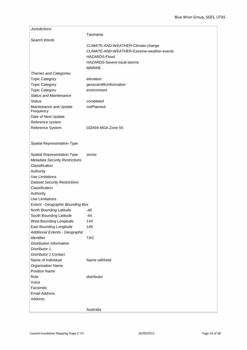
Blue Wren Group, SGES, UTAS
Coastal Inundation Mapping Stage 2 V1 26/09/2012 Page 33 of 38
Jurisdictions
Tasmania
Search Words
CLIMATE-AND-WEATHER-Climate-change
CLIMATE-AND-WEATHER-Extreme-weather-events
HAZARDS-Flood
HAZARDS-Severe-local-storms
MARINE
Themes and Categories
Topic Category elevation
Topic Category geoscientificInformation
Topic Category environment
Status and Maintenance
Status completed
Maintenance and Update Frequency
notPlanned
Date of Next Update
Reference system
Reference System GDA94 MGA Zone 55
Spatial Representation Type
Spatial Representation Type vector
Metadata Security Restrictions
Classification
Authority
Use Limitations
Dataset Security Restrictions
Classification
Authority
Use Limitations
Extent - Geographic Bounding Box
North Bounding Latitude -40
South Bounding Latitude -44
West Bounding Longitude 144
East Bounding Longitude 149
Additional Extents - Geographic
Identifier TAS
Distribution Information
Distributor 1
Distributor 1 Contact
Name of Individual Name withheld
Organisation Name
Position Name
Role distributor
Voice
Facsimile
Email Address
Address
Australia

Blue Wren Group, SGES, UTAS
Coastal Inundation Mapping Stage 2 V1 26/09/2012 Page 34 of 38
Appendix 2. CSIRO Storm Tide Modelling Evaluation of storm tide surfaces associated with 1 in 100 year return periods Author: Kathy McInnes, 2009 Extreme sea levels are comprised primarily of positive astronomical tides in conjunction with a storm surge caused by the severe winds and falling pressure associated with a severe weather event. The approach to evaluating return periods of the combination of the tide and the surge, the so-called ‘storm tide’ employed both hydrodynamic and extreme value statistical modelling techniques. The two components were modelled separately and combined using well established joint probability methods based upon Pugh and Vassie, (1980) and Tawn and Vassie (1989). The methodology for each is described below.
Storm surge Hydrodynamic modelling in this study was undertaken using the depth integrated storm surge model GCOM2D (Hubbert and McInnes, 1999). Storm surge event probabilities were estimated by simulating a population of storm surge events identified from a selection of suitably long tide gauge records. The pre-selection of extreme events in the observational records was to circumvent the need to continuously simulate sea level data over the entire length of the record but rather to simulate only the extreme events that would ultimately contribute to the estimation of storm surge return periods, thereby minimising computational requirements. This approach assumes that the scale of the meteorological disturbance is of sufficiently large spatial scale to produce a sea level response that will be captured on the tide gauge network that has been used. As discussed in McInnes et al. (2009) this is a reasonable assumption for the mid-latitude regions of Australia. It would not be a suitable approach for the tropical regions of Australia where the main driver of storm surges are the small scale and relatively short-lived tropical cyclones whose impact may not be recorded by the relatively sparse tide gauge network. For these regions, a method such as described in McInnes et al., (2003) would be more suitable. Prior to the event selection, hourly sea level data from the selected tide gauges were filtered using the method of Godin (1972) to obtain a time series of hourly sea level residuals, which closely represent the component of sea level variability due to meteorological forcing. Records of the maximum residual value occurring in each day were then derived for the tide gauges. A summary of the tide gauge records used to select extreme events is given in Table 1. These gauges were used to identify storm surges, owing to their length, completeness and distribution along the southern Australian coastline. Data gaps in these records were filled with data from alternative tide gauge records, which were selected on the basis of a high correlation with the key record being treated. Linear regression relationships were established between the key record and each of the alternative records and these were used to scale the data being used to fill data gaps prior to insertion into the key record. Hence systematic differences between the key record and alternative records were accounted for.
Table 1: Summary of the tide gauge records used for event selection in each state.
Station name State Approximate No. of years
Start date
End date
Threshold cm
Brisbane QLD 20 1986 2005 21
Gold Coast QLD 20 1986 2005 18
Coffs Harbour NSW 20 1986 2005 19
Sydney NSW 20 1986 2005 19
Batemans Bay NSW 20 1986 2005 22
Lakes Entrance VIC 37 1966 2003 14
Point Lonsdale VIC 37 1966 2003 20
Portland VIC 37 1966 2003 15
Georgetown TAS 37 1966 2003 19
Hobart TAS 37 1966 2003 22
Adelaide SA 37 1966 2003 40
Esperance WA 37 1967 2004 25
Freemantle WA 37 1967 2004 28
Port Hedland WA 37 1967 2004 16

Blue Wren Group, SGES, UTAS
Coastal Inundation Mapping Stage 2 V1 26/09/2012 Page 35 of 38
A population of independent storm surge events suitable for extreme event analysis was identified from the complete key time series of residuals on a state-by-state basis. An event was defined as an episode
during which daily maximum residual values exceeded a threshold, , above a background level. The
value of that was used in each case was selected conservatively to yield a population of events that included all of the extreme events in the time series without being overly conservative such that multiple independent events were represented as single events. The selection of the threshold required knowledge of the typical meteorological drivers of extreme sea levels in the different regions and their associated time scales. These are described in McInnes and Hubbert (2001), McInnes et al., (2001) and McInnes and Hubbert, (2003) for the south and east coasts. The population also included many events that were not extreme. These had no impact on the results of the subsequent extreme value analysis since they were not used. For each state, events identified in different key time series used for that state that overlapped in time were regarded as a single event, the assumption being that they were the result of a single weather system propagating through the region. For each state indicated in Table 1, the population of selected events was modelled with GCOM2D with atmospheric forcing only. The 10 m winds and mean sea level pressures required to force the hydrodynamic model were obtained from the US National Center for Environmental Prediction (NCEP)
reanalyses (Kalnay et al., 1996). Wind fields were available on a 1.875°1.875° global grid and mean
sea level pressure fields were available on a 2.5°2.5° global grid every 6 hours from 1958 onwards. The NCEP data were interpolated spatially to each of the GCOM2D grids. Modelling was carried out over a 5 km grid shown in Figure 1 for all states except Victoria for which modelling was also carried out at 1 km resolution as described in McInnes et al., (2009). At the termination of the simulation of each storm surge event, the maximum sea level attained at each model gridpoint throughout the simulation, hereafter referred to as the “storm surge height”, and was stored for later analysis.
Figure 1: Region over which hydrodynamic modelling was undertaken on a 5 km resolution grid. Since the population of storm surge events identified in the tide gauge records represents an interval of time that is shorter than the return period for which extreme sea level heights are being sought, extreme value statistical techniques were used to extrapolate from the data set to estimate probabilities for extreme storm surge heights with longer average recurrence intervals. Experimentation with different approaches (see McInnes et al., 2009) yielded the r-largest Generalized Extreme Value distribution (GEV) (see Coles, 2001), in which the highest 2 events to occur each year are fitted to the distribution, as being the most suitable method for use in this study.
Astronomical Tides Astronomical tide constituents are available at the locations of tide gauges around Australia. However for the purposes of developing continuous surfaces of tide height, hydrodynamical modelling was used to generate tidal information on a grid comparable to that used for the storm surge modelling. The three-dimensional counterpart to GCOM2D (GCOM3D) was used for this purpose. GCOM3D (Hubbert 1993, 1999) calculates water currents in both the horizontal and vertical planes. This is important for representing tides accurately because seabed friction affects the vertical gradient of tidal currents and hence the phase and amplitude of tides at the coast.

Blue Wren Group, SGES, UTAS
Coastal Inundation Mapping Stage 2 V1 26/09/2012 Page 36 of 38
Model simulations were carried out for several months using tidal heights from a global tidal model (Le Provost et al., 1995) as deep water boundary conditions. The time series of tide heights were then subjected to analysis at each model grid point to obtain an improved set of tidal phases and amplitudes. An iterative approach was adopted that involved running the model over several tidal cycles, calculating the root mean square errors of phase and amplitude of the modelled constituents at locations where tide gauge data existed and adjusting the boundary conditions until the RMS errors were minimised. Frequency histograms for the tidal heights were then developed for the location of each grid point of the storm surge domain by running a tide model (Foreman, 1977) over a full astronomical (18.6 year) cycle using the derived tidal constituents.
Estimation of storm tide return periods The common approach for combining the tidal distributions with those of storm surges is to assume independence between the tide and surge distributions. This is a reasonable assumption in cases where water depths are very much greater than the tidal range. Along much of the coastline under consideration in southern Australia this is a reasonable assumption. The approach, commonly referred to as the “joint probability” method (Pugh and Vassie, 1980), allows the convolution of the two probability distributions for tide and surge height (see also Tawn and Vassie, 1989). Formally this is written as
dtPPtP TS
)()()( (1)
where PS and PT represent the probability distributions for surge and tide respectively. The convolution of two probability distributions is equivalent to the probability distribution of the sum of the two independent random variables. An equivalent (and in some respects simpler) approach to convolving the tide and surge distributions is to employ a Monte-Carlo approach to randomly sample a population of tide and surge values that are summed to develop a storm tide probability distribution. A practical advantage of combining the two distributions in this way rather than undertaking a more formal mathematical convolution of the two probability or frequency distributions is that the interval widths of the two distributions do not need to be identical. Total sea levels were estimated using the Monte-Carlo approach in which 200 sets of 1000 storm tides were sampled to enable the evaluation of both average storm tide height and 95% confidence limits. The sea level totals were ranked from largest to smallest and the return levels were calculated using R = N / r where R is the return level, N is the number of random samples and r is the rank of the event. The methodology used in this study is illustrated schematically in Figure 2 for the Victorian coast. This illustrates the spatial pattern of the estimated 1 in 100 year storm surge height over this region with the largest surges occurring within Western Port Bay. Also shown is the 99
th percentile tide height from the
tide frequency histogram indicating that the highest tides occur in central Bass Strait. The 1 in 100 year storm tide surface reflects how the contributions from the tides and surge combine to produce the highest storm tides on the coastline between Western Port Bay and Wilson’s Promontory. On the other hand, in Port Phillip Bay, where the magnitude of the 1 in 100 year storm surge is similar to that on the adjacent Bass Strait coastline, the combination with tides (which are considerably attenuated within Port Phillip Bay) yields lower 1 in 100 year storm tides compared to the adjacent Bass Strait coastline. The storm tide values as represented in Figure 2 for the Victorian coastline, were then interpolated to a series of latitude and longitude coordinates which represent the Smartline, that has been generated for the National Coastal Vulnerability Assessment, which comprises a line of points around the coastline of Australia to which a range of coastal characteristics and attributes such as 1 in 100 year storm tide height can be assigned..

Blue Wren Group, SGES, UTAS
Coastal Inundation Mapping Stage 2 V1 26/09/2012 Page 37 of 38
Predic tion of tides over 18.6 years
to develop tide height frequencies
Evaluation of high resolution tide
constituents from modelled tides
Simulation of several tidal cyc les
with hydrodynamic model
Combine
surge and tides
using the joint probability
methodExtreme value statistical analysis to
evaluate storm surge probabilities
Simulation of storm surges with
hydrodynamic model
Selection of storm surge events
from tide gauge records
25 km 25 km 25 km25 km
100 km
1 in 100 year storm surge
100 km
1 in 100 year storm tide
100 km
99th percentile tide height
(metres)
(metres)
(metres) Figure 2: Schematic diagram illustrating the methodology used to evaluate storm tide return periods. The illustrations present examples of the spatial variation of the 1 in 100 year storm surge and storm tide surfaces and the 99
th percentile tide height.
References
Foreman, G. G.: Manual for Tidal Heights Analysis and Prediction, Pacific Marine Science Report 77-
10, Institute of Ocean Sciences, Victoria, Canada, 98pp., 1977. Godin, G.: The Analysis of Tides. University of Toronto Press, Toronto, Canada, 1972. Hubbert, G. D., and McInnes, K. L.: A storm surge inundation model for coastal planning and impact
studies, J. Coastal Res., 15, 168-185, 1999. Hubbert, G.D. 1993: Modelling continental shelf flows along the New South Wales coast with a fully
three dimensional ocean model. Proc. 11th Australasian Coastal and Ocean Engineering Conference, Townsville, Australia.
Hubbert, G.D. 1993: Oil spill trajectory modelling with a fully three dimensional ocean model. Proc. 11th Australasian Coastal and Ocean Engineering Conference, Townsville, Australia.
Hunter, J., 2010: Estimating Sea-Level Extremes Under Conditions of Uncertain Sea-Level Rise, Climatic Change, 99:331-350, DOI:10.1007/s10584-009-9671-6.
(http://staff.acecrc.org.au/~johunter/climatic_change_2009_distributable_version.pdf) IPCC, 2007: Climate change 2007: the physical science basis. In: Contribution of working group I to the fourth assessment report of the intergovernmental panel on climate change, Cambridge University Press, Cambridge. Kalnay, E., Kanamitsu, M., Kistler, R., Collins, W., Deaven, D., Gandin, L., Iredell, M., Saha, S., White,
G., Woollen, J., Zhu, Y., Leetmaa, A., Reynolds, B., Chelliah, M., Ebisuzaki, W., Higgins, W., Janowiak, J., Mo, K. C., Ropelewski, C., Wang, J., Jenne, R., and Joseph, D.: The NCEP/NCAR 40-year reanalysis project, B. Am. Meteorol. Soc., 77, 437–471, 1996.
Le Provost, C. Bennet, A.F. and Cartwright D.E. 1995: Ocean tides for and from TOPEX/POSEIDON. Science 267; 639-642.

Blue Wren Group, SGES, UTAS
Coastal Inundation Mapping Stage 2 V1 26/09/2012 Page 38 of 38
McInnes, K.L., Macadam, I., Hubbert, G.D. and O’Grady, J.G. 2009: A Modelling Approach for Estimating the Frequency of Sea Level Extremes and the Impact of Climate Change in Southeast Australia. Natural Hazards DOI 10.1007/s11069-009-9383-2
McInnes, K.L. and Hubbert, G.D. 2003: A numerical modeling study of storm surges in Bass Strait. Aust. Met. Mag. 52. 143-156.
McInnes, K.L., K.J.E. Walsh, G. D. Hubbert and T. Beer, 2003: Impact of Sea-level Rise and Storm Surges on a Coastal Community. Nat. Haz. 30(2) 187-207.
McInnes, K.L., D.J. Abbs, G. D. Hubbert and S. E. Oliver, 2002: A Numerical Modelling Study of Coastal Flooding. Meteorol. Atmos. Phys. 80, 217-233.
McInnes, K.L. and Hubbert, G.D. 2001: The impact of eastern Australian cut-off lows on coastal sea levels. Meteorological Applications, 8, 229-243.
Pugh, D. T., and Vassie, J. M.: Applications of the joint probability method for extreme sea level computations, P. I. Civil Eng. Part 2, 69, 959-975, 1980.
Tawn, J. A., and Vassie, J. M.: Extreme sea levels: the joint probabilities method revisited and revised, P. I. Civil Eng. Part 2, 87, 429-442, 1989.