Coastal jet adjustment near Point Conception, CA with

KU ScholarWorks | http://kuscholarworks.ku.edu

Coastal jet adjustment near

Point Conception, CA with

opposing wind in the bight

by David Rahn, Thomas Parish and David Leon

KU ScholarWorks is a service provided by the KU Libraries’ Office of Scholarly Communication & Copyright.

This is the published version of the article, made available with the permission of the publisher. The original published version can be found at the link below.

Rahn, David A. et al. (2014). Coastal jet adjustment near Point Conception, CA with opposing wind in the bight. Monthly Weather Review 142:1344-1360

Published version: http://dx.doi.org/10.1175/MWR-D-13-00177.1

Terms of Use: http://www2.ku.edu/~scholar/docs/license.shtml

Please share your stories about how Open Access to this article benefits you.

2013

Coastal Jet Adjustment near Point Conception, California, with OpposingWind in the Bight

DAVID A. RAHN

Atmospheric Science Program, Department of Geography, University of Kansas, Lawrence, Kansas

THOMAS R. PARISH AND DAVID LEON

Department of Atmospheric Science, University of Wyoming, Laramie, Wyoming

(Manuscript received 29 May 2013, in final form 29 October 2013)

ABSTRACT

Typical spring and summer conditions offshore of California consist of strong northerly low-level wind

contained within the cool, well-mixedmarine boundary layer (MBL) that is separated from the warm and dry

free troposphere by a sharp temperature inversion. This system is often represented by two layers constrained

by a lateral boundary. Aircraft measurements near Point Conception, California, on 3 June 2012 during the

PrecisionAtmosphericMBLExperiment (PreAMBLE) captured small-scale features associatedwith northerly

flow approaching the point with the added complexity of encountering opposing wind in the Santa Barbara

Channel. An extremely sharp cloud edge extends south-southwest of Point Conception and the flight strategy

consisted of a spoke pattern to map the features across the cloud edge. Lidar and in situ measurements reveal

a nearly vertical jump in theMBL from500 to 100m close to the coast and a sharp edge at least 70kmaway from

the coast. In this case, it is hypothesized that it is not solely hydraulic features responsible for the jump, but the

opposing flow in the Santa Barbara Channel is a major factor modifying the flow. Just southeast of Point

Conception are three distinct layers: a shallow, cold layer near the surface with northwesterly winds associated

with an abrupt decrease in MBL height from the north that thins eastward into the Santa Barbara Channel;

a cool middle layer with easterly wind whose top slopes upward to the east; and the warm and dry free tro-

posphere above.

1. Introduction

Strong wind near the surface along the Californian

coast is common in the spring and is ultimately set up by

the contrast in pressure between the thermal low over

the southwest United States and the anticyclone over the

cool Pacific Ocean. Associated with the subtropical

branch of the Hadley circulation is downward motion

that maintains a strong subsidence inversion that caps

the marine boundary layer (MBL). During the spring

and summer a general wind speed maximum extends

along the California coast from CapeMendocino to past

Point Conception with a local maximum in the lee of

Point Conception. Transient synoptic systems may also

contribute to particularly strong wind events along the

Southern California shoreline. Localized maxima of

wind speed are embedded within the broader low-level

jet and occur along the coastline near changes in the

orientation of the topography such as points and capes.

The alongshore variability of the wind and other im-

portant parameters is described in depth by Dorman

et al. (2000), Kora�cin and Dorman (2001), and Kora�cin

et al. (2004).

The Froude number (Fr) is an important diagnostic

variable for coastal flow. It is the ratio of the flow speed

to the fastest possible gravity wave in the layer, which is

proportional to MBL height and strength of the in-

version. Typically, if the wind is strong within a shallow

MBL, local variation along the coast is often attributed

to mechanical forcing (e.g., Edwards et al. 2001; Haack

et al. 2001). Strictly speaking in the ideal case, Fr of unity

is transcritical. The calculation and meaning of Fr is

imprecise in the real atmosphere because of departures

from shallow-water theory. The ideal case is a homoge-

neous, single-layer fluid, while the real atmosphere is

Corresponding author address: David A. Rahn, Atmospheric

Science Program, Department of Geography, University of Kansas,

1475 Jayhawk Blvd., 201 Lindley Hall, Lawrence, KS 66045-7613.

E-mail: [email protected]

1344 MONTHLY WEATHER REV IEW VOLUME 142

DOI: 10.1175/MWR-D-13-00177.1

� 2014 American Meteorological Society

mailto:[email protected]

variably stratified. However, it is the relative numbers

that are important (Burk and Thompson 2004). For ex-

ample, Rogerson (1999) showed that an expansion fan

occurs if the approaching marine layer flow has Fr be-

tween 0.5 and 1. Mechanical features manifest as a com-

pression bulge upwind of a cape as the flow slows and the

MBL deepens, while an expansion fan occurs downwind

of a cape as the flow speeds up and the MBL thins. These

features are tied to the topography and are on the order

of 10 km (Kora�cin and Dorman 2001). Features that

resemble compression bulges and expansion fans have

been observed by aircraft from Cape Blanco to Point Sur

(Winant et al. 1988;Rogers et al. 1998;Dorman et al. 1999)

and Point Conception using surface stations (Dorman and

Winant 2000) and a numerical model (Skyllingstad et al.

2001). In addition, many modeling studies investigate

mechanical features (e.g., Samelson 1992; Burk and

Thompson 1996; Rogers et al. 1998; Burk et al. 1999;

Rogerson 1999; Tjernstr€om and Grisogono 2000).

Dorman and Kora�cin (2008) provide a particularly

detailed analysis of the conditions near Point Concep-

tion, California, using surface observations, soundings,

radar profilers, and high-resolution numerical simula-

tions. They conclude that the synoptic setting is what

fundamentally drives the northerly flow, and thatmarine

layer hydraulic dynamics force the responses of a slow-

ing and deepening of the layer upwind and a quickening

and thinning of the layer downwind of the point. Al-

ternate explanations that may force these features such

as a diurnal thermal low or leeside flow down the Santa

Ynez Mountains were deemed unacceptable.

Important details of this system are often missed be-

cause of the small-scale nature and difficultly in observing

these features at a sufficiently high spatial resolution

offshore near the top of the MBL. To address this issue,

a field project called the Precision Atmospheric MBL

Experiment (PreAMBLE) was designed to study such

details of the lower atmosphere in the vicinity of the ex-

treme bend near Point Conception. Few aircraft obser-

vations have been obtained offshore of Point Conception,

but previous campaigns include Edinger and Wurtele

(1972) and Rogers et al. (1998). Another case of a coastal

jet on 19 May 2012 during PreAMBLE has been exam-

ined by Rahn et al. (2013), which had a transition of

the northerly coastal flow around Point Conception un-

der relatively stagnant conditions in the Santa Barbara

Channel. The classic features described by the literature

were present in the 19 May 2012 case, but other features

such as the dilution of the temperature inversion as the

MBL thins and off-continent flow above the MBL were

highlighted with in situ and lidar data. In addition to the

coastal jet, a prominent cyclonic circulation (the Catalina

eddy) may develop in the California Bight, which is most

frequent from late spring through early fall and has

a regular diurnal cycle (Mass and Albright 1989).

The Catalina eddy and northerly flow around Point

Conception are commonly treated separately. This

work examines a case when there are strong winds

transitioning around the point at the same time there is

an opposing wind associated with a cyclonic circulation

in the California Bight. Measurement systems and

techniques are introduced in section 2. Results from the

observations are shown in section 3 and are synthesized

into a conceptual model at the end of that section. The

main conclusions are briefly summarized in section 4.

2. Data

PreAMBLE used the University of Wyoming King

Air (UWKA) as the primary observational platform and

was based out of the Naval Air Station at Point Mugu,

California, from 15 May to 17 June 2012. The vertical

structure offshore is observed in situ by the UWKA as

the aircraft ascends and descends. By flying on an iso-

baric surface and measuring the height, the UWKA can

precisely map the horizontal pressure gradient force

(PGF). Since the slope of the isobaric surface is related

to the PGF, this is a critical component in diagnosing the

forcing of atmospheric motion. Early work employed

radar altimeters to obtain the height measurements

(e.g., Rodi and Parish 1988), but more recently differ-

ential GPS processing is used because it provides a more

accurate measurement (Parish et al. 2007). The gentle

slope of an isobaric surface requires that the height

needs to be known to within a fraction of a meter. For

example, a 10m s21 geostrophic wind at 438N is associ-

ated with an isobaric height change of 10 cm every

kilometer. Precise measurements are critical. The air-

craft autopilot deviates off of the exact isobaric surface,

but any deviation is corrected with the hypsometric

equation that also requires an accurate static pressure

measurement. This technique has been proven in pre-

vious cases (e.g., Rahn and Parish 2007) and details can

be found in Parish et al. (2007) and Parish and Leon

(2013). An additional concern in applying this method is

that any pressure change over time during the flightmust

be known since it would alter the slope. Simply flying

reciprocal legs alleviates this problem since repeating

the same leg in the opposite direction reveals any time

tendency that can be corrected given the measured rate

of change of height with time.

Part of the instrument payload on the UWKA dur-

ing PreAMBLE was the Wyoming Cloud lidar (WCL),

which was configured with upward- and downward-

looking beams. The WCL is a 355-nm lidar designed for

retrieval of cloud and aerosol properties. The returned

MARCH 2014 RAHN ET AL . 1345

signal for the upward-looking lidar is sampled at 3.75-m

intervals, while the signal for the downward-looking li-

dar is sampled at 1.5-m intervals. Additional details of

the WCL can be found in Wang et al. (2009) and Wang

et al. (2012). The lidar data are combined with inertial

navigation system/GPS data from the UWKA to pro-

duce time-height images of the (uncalibrated) attenu-

ated backscatter. The WCL is well suited to determine

cloud boundaries, but because the lidar signal is rapidly

attenuated in cloud, the lidars are unable to penetrate

deeply into the cloud layer. Lidar data have been col-

lected in the past during Coastal Waves 1996 (Rogers

et al. 1998); however, an important advancement is the

depolarization ratio, which assisted in the interpretation

of the transition region.

3. Results

a. Overview

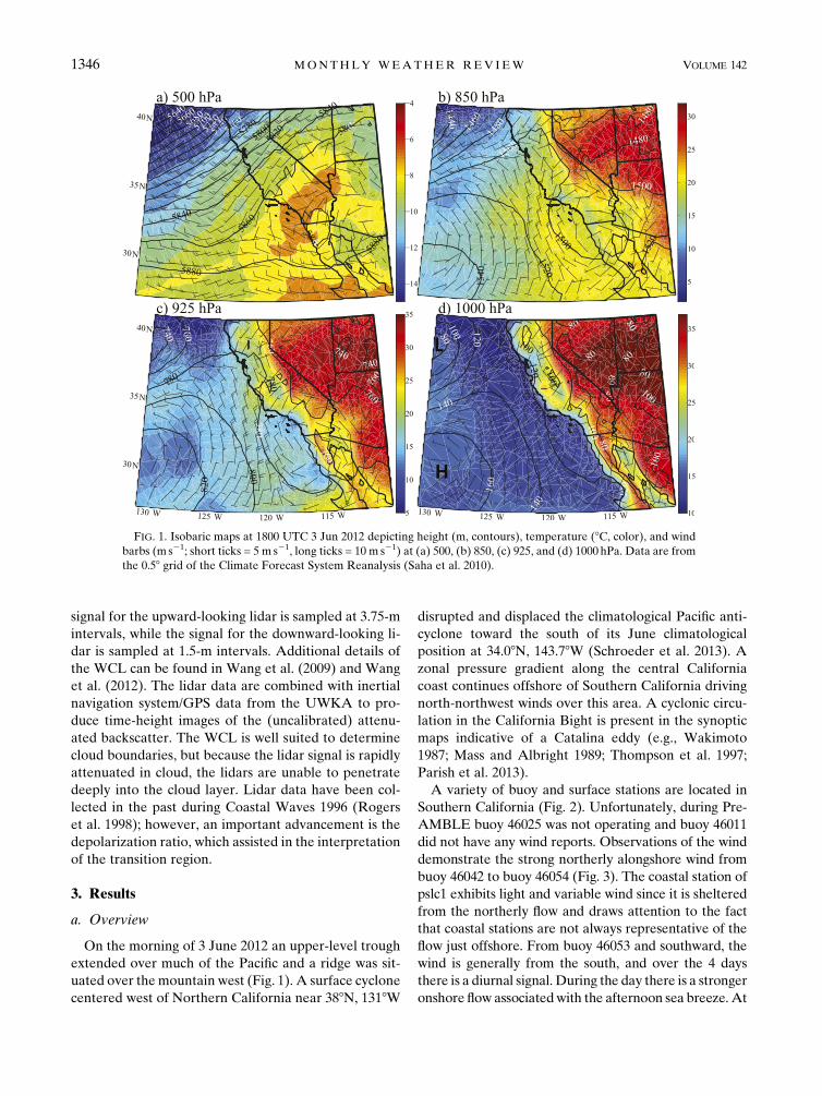
On the morning of 3 June 2012 an upper-level trough

extended over much of the Pacific and a ridge was sit-

uated over themountain west (Fig. 1). A surface cyclone

centered west of Northern California near 388N, 1318W

disrupted and displaced the climatological Pacific anti-

cyclone toward the south of its June climatological

position at 34.08N, 143.78W (Schroeder et al. 2013). A

zonal pressure gradient along the central California

coast continues offshore of Southern California driving

north-northwest winds over this area. A cyclonic circu-

lation in the California Bight is present in the synoptic

maps indicative of a Catalina eddy (e.g., Wakimoto

1987; Mass and Albright 1989; Thompson et al. 1997;

Parish et al. 2013).

A variety of buoy and surface stations are located in

Southern California (Fig. 2). Unfortunately, during Pre-

AMBLE buoy 46025 was not operating and buoy 46011

did not have any wind reports. Observations of the wind

demonstrate the strong northerly alongshore wind from

buoy 46042 to buoy 46054 (Fig. 3). The coastal station of

pslc1 exhibits light and variable wind since it is sheltered

from the northerly flow and draws attention to the fact

that coastal stations are not always representative of the

flow just offshore. From buoy 46053 and southward, the

wind is generally from the south, and over the 4 days

there is a diurnal signal. During the day there is a stronger

onshore flow associatedwith the afternoon sea breeze. At

FIG. 1. Isobaric maps at 1800 UTC 3 Jun 2012 depicting height (m, contours), temperature (8C, color), and wind

barbs (m s21; short ticks = 5 m s21, long ticks = 10 m s21) at (a) 500, (b) 850, (c) 925, and (d) 1000 hPa. Data are from

the 0.58 grid of the Climate Forecast System Reanalysis (Saha et al. 2010).


the offshore buoys 46069 and 46047 the wind was con-

sistently from the northwest, and at 46086 the wind was

westerly from 0000 UTC 1 June to 1200 UTC 2 June and

light and variable afterward (not shown).

Observations of mean sea level pressure along the coast

are shown in Fig. 4. To eliminate the influence of pressure

tides on the 10-h evolution, the average diurnal cycle of

surface pressure is removed. The surface pressure along

the coast reveals that from 1200 to 2200 UTC there is an

alongshore pressure gradient pointed toward the south

from buoy 46042 to pslc1. At 1200 UTC there is also

an alongshore pressure gradient pointed to the south un-

til icac1, but the pressure increases at iiwc1. Over the

morning and into the afternoon, the pressure gradient

from iiwc1 to ntbc1 reverses such that there is an along-

shore pressure gradient pointed to the north. In the af-

ternoon when the flight took place, there are opposing

alongshore pressure gradients with a local pressure max-

imum at ptgc1 that is ;1hPa greater than the nearby

stations of pslc1 and ntbc1.

Preflight conditions suggested the development of

a sharp cloud boundary throughout the morning as ini-

tially inferred from an animation of satellite imagery.

Morning cyclonic circulation in the Southern California

Bight was common during the field campaign, but varied

in extent and intensity and often dissipated before the

late afternoon when a majority of the flights took place.

The flight strategy for thismissionwas tomap the isobaric

surface along the cloud edge by flying a spoke pattern

emanating from a point halfway between Point Concep-

tion and San Miguel Island on the western edge of the

Santa Barbara Channel (Fig. 5). This pattern was flown

along an isobaric surface in one direction startingwith the

first leg in set A followed by additional isobaric legs far-

ther south with a sounding at the end of the final pattern

leg at E. After the sounding, the pattern was repeated in

reverse. While airborne, air traffic control allowed the

flight plan to be modified toward the end by terminating

the return leg of set B early and allocating that flight time

FIG. 2. Locations of buoy and coastal surface stations.

FIG. 3. Surface wind vectors (m s21, scale at top right) at buoy

and surface stations along the California coast that are indicated at

the top left of each time series.


to instead fly above the clouds and use the downward-

pointing lidar to continuously detect the MBL top as it

abruptly dropped in height along set A. During the ferry

through the Santa Barbara Channel to and from the

center of the spoke pattern, the aircraft performed a se-

ries of ascents and descents culminating in a sawtooth

pattern to obtain the vertical structure. Measurements

from the individual isobaric legs are discussed first and

then after examining the aircraft soundings, a broader

conceptual model is proposed that synthesizes the avail-

able data.

b. Isobaric legs

Measurement of the height change with distance

along an isobaric surface enables the PGF to be de-

termined directly from in situ observations. To correctly

calculate the PGF, any changes of the height of the

isobaric surface over time (referred to as the height

tendency) must be taken into account since it can skew

the data toward stronger or weaker PGF than reality

(Rodi and Parish 1988). Height tendency is typically

attributed to synoptic-scale features and can be applied

to the entire flight. To alleviate this problem, the spoke

pattern was not only repeated flying in the opposite

direction to get an isobaric tendency, but the aircraft

passed over the same point at the center of the spoke

pattern at the end of every leg. Isobaric heights fell at an

average rate of 0.0007m s21. This cannot be neglected

because it corresponds to a height fall of 7.5m over a 3-h

period. Flight time for this mission was 3.7 h. The fol-

lowing analysis takes the height tendency into account

by correcting the isobaric height by 0.0007m s21 times

the number of seconds from the beginning of the first

leg of the set.

Beginning with the reciprocal set of legs closest to the

coast (set A), it is not surprising that a large gradient in

the isobaric surface (Fig. 6) exists close to the terrain

based on the standard conceptual model of an expansion

fan (e.g., Winant et al. 1988; Dorman and Kora�cin 2008)

and other flights during PreAMBLE (Rahn et al. 2013).

In the north the isobaric surface rises, which implies

a deeper MBL. Concurrently, the wind speed decreases,

FIG. 4. Surface pressure (hPa) on 3 Jun 2012 every 2 h along the

coast with the average diurnal cycle removed. Distance (km) is

calculated by following the coastline and locations of the obser-

vations are indicated on the bottom.

FIG. 5. (left) Topographic elevation (m) and flight track on 3 Jun 2012. Location of soundings along the flight track

are indicated by colors and labeled with S and the sounding number. (right) Visible satellite image at 2100UTC 3 Jun

2012 with the flight tracks overlaid.


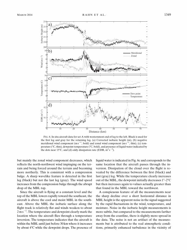
but mainly the zonal wind component decreases, which

reflects the north-northwest wind impinging on the ter-

rain and being forced around the terrain and becoming

more northerly. This is consistent with a compression

bulge. A sharp wavelike feature is detected in the first

leg (black) but not the last leg (gray). The wind speed

increases from the compression bulge through the abrupt

drop of the MBL top.

Since the aircraft is flying at a constant level and the

top of theMBL lowers rapidly toward the southeast, the

aircraft is above the cool and moist MBL in the south-

east. Above the MBL the isobaric surface along the

flight track is relatively flat and winds weaken to about

2m s21. The temperature and dewpoint clearly mark the

location where the aircraft flies through a temperature

inversion. The temperature indicates that the aircraft is

within theMBL until just before 30kmwhere it increases

by about 48C while the dewpoint drops. The presence of

liquid water is indicated in Fig. 6c and corresponds to the

same location that the aircraft passes through the in-

version. Dissipation of the cloud over the flight is re-

vealed by the difference between the first (black) and

last (gray) leg. While the temperature clearly increases

out of theMBL, the dewpoint initially decreases 18–28Cbut then increases again to values actually greater than

that found in the MBL toward the northwest.

A conspicuous feature of all the measurements near

the sharp decline over a short horizontal distance in

MBL height is the apparent noise in the signal suggested

by the rapid fluctuations in the wind, temperature, and

moisture. Noise in the isobaric height measurements is

more subtle, but compared to the measurements farther

away from the coastline, there is slightly more spread in

the data. The noise is not an artifact of the measure-

ments but is attributed to the real atmospheric condi-

tions, primarily enhanced turbulence in the vicinity of

FIG. 6. In situ aircraft data for set A with westernmost end of leg to the left. Black is used for

the first leg and gray for the returning leg. (a) Corrected isobaric height (m), (b) negative

meridional wind component (m s21, bold) and zonal wind component (m s21, thin), (c) tem-

perature (8C, thin), dewpoint temperature (8C, bold), and presence of liquid water indicated by

the dots near 158C, and (d) eddy dissipation rate (EDR, m2 s23).


the sharp MBL height drop and large wind shear. The

eddy dissipation rate (EDR) is a measure of turbulence

using the method developed by MacCready (1964) with

higher values corresponding to more turbulence. There

is a spike in turbulence as the aircraft crosses the tem-

perature inversion and encounters large changes in wind

speed and direction. Thus, the greater EDR values are

likely enhanced by the mechanical generation of tur-

bulence by wind shear. Toward the southeast, the tur-

bulence decreases but there are noticeable spikes such

as at 60 km in the second (gray) leg. Soundings shown

later also indicate a large vertical wind shear near this

flight level that contributes to the mechanical pro-

duction of turbulence.

In each of the isobaric legs of the spoke pattern there

is a continuous transition from north to south. For brev-

ity, only sets A, C, and E are shown. Observations from

set C (Fig. 7) depict many of the same features although

the transition from west to east is less pronounced. A

small jump in the isobaric height is present at ;15km in

both legs with the second leg exhibiting a slightly more

prominent jump. An increase of temperature near 18km

is associated with the cloud edge. Enhanced turbulence

is again evident in the fluctuations of all the variables,

but measurements of EDR indicate a slightly lower

value than set A. Once again, the dewpoint temperature

increases toward the east after the aircraft passes

through the temperature inversion. Another difference

with the previous legs is that toward the extreme east

end of the leg the wind is from the east.

Set E comprises the southernmost isobaric legs di-

rected along a northeast–southwest axis and theUWKA

reaches the sharp cloud edge at the western end of the

leg (Fig. 8). The isobaric height is linear with little indi-

cation of any sort of jump. Bothwind components decrease

linearly toward the northeast. Winds are ;10ms21 from

the north-northwest along the western portion of the leg.

At the eastern end of the leg, wind directions have

switched to easterly at ;2ms21. Geostrophic wind per-

pendicular to the flight track (roughly northwest) is

13m s21, so the wind is subgeostrophic and should ac-

celerate toward the east, but the acceleration of the

flow is against an easterly wind. After passing through

a weak increase of temperature, the dewpoint increases

FIG. 7. As in Fig. 6, but for set C.


to values above that found in the MBL to the southwest.

Turbulence is slightly elevated, but a region of reduced

turbulence is found near a distance of 20km that is also

reflected in the temperature and windmeasurements that

show less variance.

c. Synthesis of isobaric measurements

There are several important features that the isobaric

legs illustrate. In set A the locally deeper MBL and

slower flow that is deflected around the cape is consis-

tent with a compression bulge northwest of the point.

Set A also contains the most pronounced changes in-

cluding a 4-m drop in the isobaric height over a hori-

zontal distance of just ;15 km. For perspective, the

geostrophic wind associated with that height gradient

is 33m s21. According to the Bernoulli equation, when

the MBL decreases in height, the wind speed increases.

This is exactly the case here where the wind increases

from 6m s21 in the northwest to 8m s21 as the MBL

depth decreases. Part of the motivation for flying the

spoke pattern was to directly measure the isobaric

heights, which enables a spatial depiction of the height

field. Figure 9 illustrates the isobaric heights from the

first entire spoke pattern that are corrected for time

tendencies and interpolated between the legs. Isobaric

height clearly drops from the northwest into the Santa

Barbara Channel. A relatively flat isobaric surface exists

near the center of the spoke pattern since the aircraft

exited the northern MBL, which has much greater hor-

izontal variability in the western region.

Measurements of the isobaric height indicate a con-

centrated zonal gradient of isobaric height that is con-

sistent with the sharp cloud edge. As seen in the

individual sets of legs (Figs. 6–8), the largest isobaric

height gradient is encountered during set A. To the

south the height gradient is weaker, but is still associated

with the cloud edge. In sets C and E, the features are

similar to set A, although not as well defined. Isobaric

height contours indicate a compression bulge just north-

west of the point since there are locally high heights,

which also appear to be detached from the high heights

farther toward the south. The localized nature of the high

FIG. 8. As in Fig. 6, but for set E.


heights north of the cape is consistent with the idea that

mechanical features such as a compression bulge do not

extend far from the topography and are on the order of

10km or so (Kora�cin and Dorman 2001). While me-

chanical features play the greatest role near the coast,

observations suggest that other features may be respon-

sible for the sharp cloud edge that extends much farther

to the south. Furthermore, the large jump in the isobaric

height as detected in set A is unlikely to be so sharp from

mechanical effects alone, and other factors may be con-

tributing, such as an interaction with the opposingwind in

the Santa Barbara Channel.

d. Vertical structure

A lidar can readily identify features of the lower

atmosphere, especially the top of the MBL and any

cloud-free layers. Because clouds northwest of Point

Conception quickly attenuated the lidar signal during

the low-level isobaric legs, an additional flight leg along

the same flight track as set A but above the MBL at

about 700m was flown to obtain a continuous mea-

surement of the MBL height from the downward beam

of the WCL (Fig. 10). From the farthest point to the

northwest the MBL depth increased to a maximum near

2325:00 UTC before slightly decreasing in height. At

2323:30 UTC the cloud ended abruptly, consistent with

the satellite imagery. The abrupt drop of theMBL height

is much sharper than the transition that occurred on

19 May 2012 under relatively quiescent conditions in the

California Bight (Rahn et al. 2013). On 19May the MBL

height dropped 200m over 20 km. The reflectivity for the

3 June case indicates a sudden drop from 400 to 100m

over just tens of meters. Figure 10 also indicates that a

low layer of high reflectivity remains below ;100m and

extends well to the southeast. There is a weaker bound-

ary in the cloud-free region to the southeast that slopes

down from500mat the far southeastern end of the domain

to 300m just before the sharp change of MBL depth. Be-

tween the nearly vertical drop of the cloud-capped MBL

to the northwest and the cloud-free boundary to the

southeast there is apparently a gap between the two

layers. The EDR indicates enhanced turbulence at

this location.

Additional lidar data from set B are used to highlight

the vertical structure. A lidar image from set B is shown

in Fig. 11 and is similar to the previous lidar image with

a few exceptions. The sharp change ofMBL height is not

continuously detected because the flight level is at ap-

proximately 200m and the beam is quickly attenuated

by droplets when flying in the cloud. Nevertheless, this

illustrates the layers in the southeastern portion more

clearly. The downward-pointing lidar detects a shallow

layer with a top near 100m, consistent with that seen in

the previous image. The upward-pointing lidar detects

a deep layer in the Santa Barbara Channel that increases

from;400m at the 2124UTC/45 kmmark and increases

to;600m at the eastern edge. A thin cloud exists at the

top of the upper layer in the far southeast, which is

present in the satellite image as well.

Three distinct layers are detected by the lidar in the

southeast. Properties of these three layers are obtained

by in situ measurements from the UWKA. On the ferry

out and back from the center of the spoke pattern, the

UWKA conducted a series of vertical ascents and de-

scents. The final descent from the outbound ferry is

depicted by the green line in the satellite image and is

just east of the lidar image. The temperature profile

above 500m reveals the classic subsidence inversion

where the temperature increases and dewpoint decreases.

The capping temperature inversion is not concentrated

in a narrow region but is fairly deep (500–800m). Below

the subsidence inversion at 500m the temperature pro-

file follows a dry adiabatic lapse rate indicating a well-

mixed layer. Just below the subsidence inversion the

dewpoint indicates saturation, consistent with the lidar

and satellite observations of a thin cloud. Below 300m

the temperature no longer follows the dry adiabatic lapse

rate and becomes a few degrees cooler than the air

above, representing another cooler, stable layer below.

Perhaps the most compelling evidence of the exis-

tence of three distinct layers is the wind profile. Wind

direction is from the northwest in both the upper layer

and lower layer. In the upper layer the wind speed ap-

proaches 10m s21. In situ measurements in the lowest

FIG. 9. Isobaric height (m) contours for the first spoke pattern

flown. Flight tracks overlaid as black dashed contours and topog-

raphy is shown using the same color scale as in Fig. 5.


layer (;150m) indicate a wind speed of ;6m s21, but

the maximum wind is likely slightly above 6m s21 since

the trend is increasing with lower height, which must

again decrease near the surface because of friction. The

change of wind direction is abrupt, though the wind

speed follows a slightly smoother transition. The most

striking feature of the wind profile is seen in the middle

layer where the wind is easterly, opposing the north-

westerly wind originating from the north of Point

Conception. The middle layer is well mixed since the

vertical profile of temperature follows a dry adiabatic

lapse rate. Wind measurements also reflect a well-

mixed middle layer since both wind speed and direction

are uniform. This layer is thought to be part of the re-

sidual circulation associated with the Catalina eddy.

This sounding is taken around buoy 46054 (Fig. 2),

which had persistent northwest wind. This really high-

lights the importance of obtaining a vertical profile that

can capture a flow moving in the opposite direction just

above the surface.

Sounding 8 was taken closer to the abrupt drop in the

MBL height near Point Conception (Fig. 5). The wind

and temperature profiles also reveal three distinct layers

(Fig. 12). The temperature profile is not as well defined

as that in Fig. 11, which may be attributed to the greater

vertical mixing associated with the larger turbulence

indicated by theEDR in the isobaric legs. Thewind speed

and direction clearly demark the transition between the

westerly flow below, southeasterly flow in themiddle, and

northwesterly flow above. The middle layer is only 100m

thick as opposed to the 250-m-thick middle layer seen in

Fig. 12, which is consistent with the lidar image that de-

tects a thicker middle layer in the east that thins toward

the west. It is also interesting to note that the wind is

actually from the southeast in the middle layer, while

sounding 11 indicated easterly wind in the middle layer.

To extend the analysis of the layers in the Santa

Barbara Channel, the sawtooth pattern flown by the

aircraft using soundings 1 through 5 is used to construct

a cross section of potential temperature and wind

(Fig. 13). The flight track is represented by the thick

dashed line and the height of the layers is marked by a

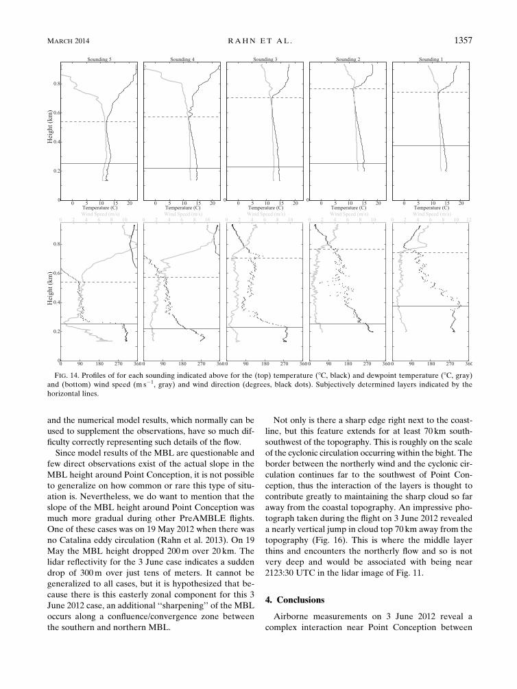
black dot. The layer heights are subjectively determined

from the individual soundings shown in Fig. 14 using

information from the temperature, dewpoint, and wind.

Some heights are not as well defined as others, but the

divisions are thought to be fairly representative of the

layers. For instance, in sounding 2 there is a discontinuity

FIG. 10. Lidar returns of (a) reflectivity (dB) and (b) depolarization (dB) over set A.West is to the left. Aircraft elevation is about 750m as

indicated by the black line near this height.


in the adiabatic profile of the temperature around 250m

and a small jump in the wind speed as well.

The meridional wind in Fig. 13 is strongest in the west

at upper levels where there is strong northwesterly flow.

In the middle layer the meridional component is light

from the south. In the lowest layer the meridional wind

is light from the north. The isentropes slope up from

west to east above 600m, consistent with the slope of the

topmost temperature inversion. Stability is near neutral

below that temperature inversion and the subtle tem-

perature changes are not as easily seen in the inter-

polated cross section then they are in the individual

profiles. However, the zonal wind displays clear differ-

ences. In the lowest layer (below ;200m) the zonal

wind is westerly and either shifts to easterly in the

middle layer or is light. There is a 4–6m s21 zonal wind

above 600m, which is easterly for soundings 1–3 and

westerly for soundings 4 and 5.

e. Numerical modeling

While this study is primarily based off of observations,

numerical models typically provide additional infor-

mation to assist in the analysis. Numerical simulations

ranging in their complexity are often used as the basis

for describing the coastal flow (Samelson 1992; Burk

and Thompson 1996; Rogers et al. 1998; Burk et al.

1999; Rogerson 1999; Tjernstr€om and Grisogono 2000;

Skyllingstad et al. 2001). Products from operational

models were used during the field campaign to support

the forecasting and guide the flight plan for the fol-

lowing day. Characteristics of the circulation in the

California bight predicted by operational models were

often diverse. For the 3 June 2012 case, the Weather

Research and Forecasting Model (WRF; Skamarock

et al. 2008) was run after the field campaign in hopes of

supplementing the observational data.

FIG. 11. (a) Visible satellite image with location of lidar image in red, sounding in green, and location of picture in Fig. 16 given by the green

circle; (b) profile of temperature (8C, red) and dewpoint temperature (8C, blue); (c) profile of wind speed (ms21, red) andwind direction (degrees,

black); and (d) lidar reflectivity (dB) with west to the left and the aircraft elevation was;0.2km as represented by the black line at that height.


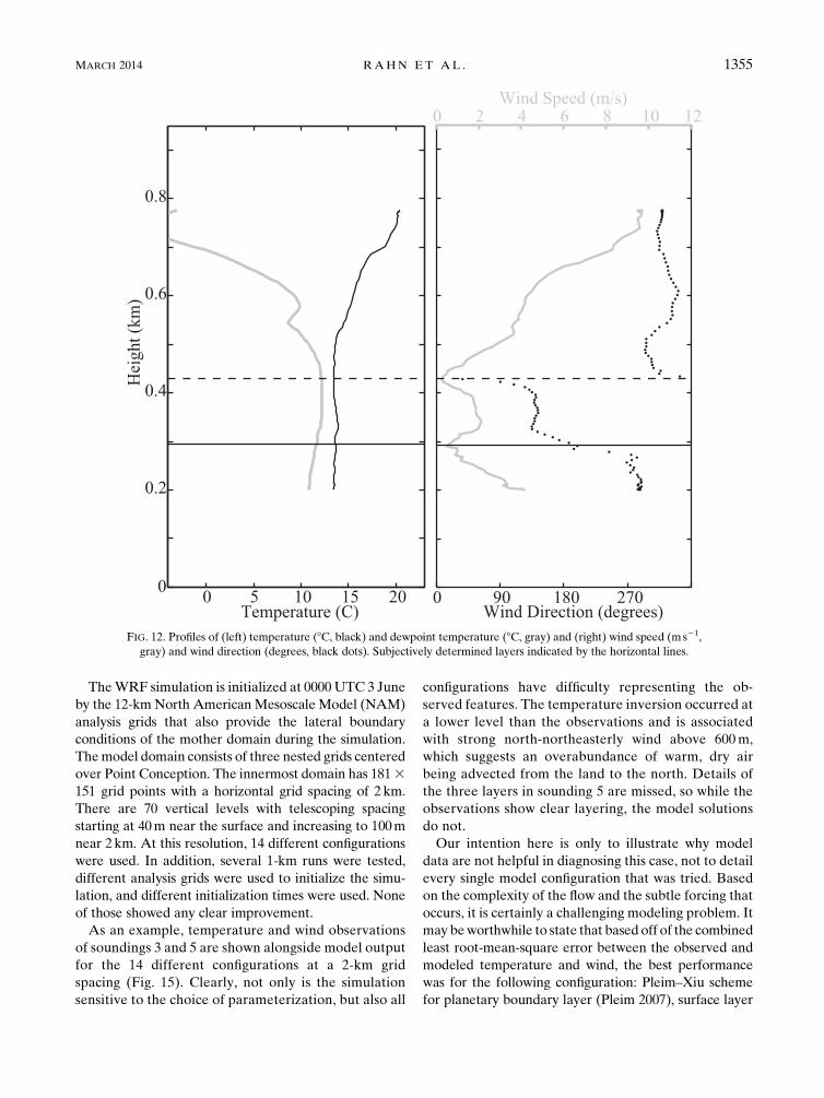
TheWRF simulation is initialized at 0000UTC 3 June

by the 12-km North American Mesoscale Model (NAM)

analysis grids that also provide the lateral boundary

conditions of the mother domain during the simulation.

Themodel domain consists of three nested grids centered

over Point Conception. The innermost domain has 1813151 grid points with a horizontal grid spacing of 2 km.

There are 70 vertical levels with telescoping spacing

starting at 40m near the surface and increasing to 100m

near 2km. At this resolution, 14 different configurations

were used. In addition, several 1-km runs were tested,

different analysis grids were used to initialize the simu-

lation, and different initialization times were used. None

of those showed any clear improvement.

As an example, temperature and wind observations

of soundings 3 and 5 are shown alongside model output

for the 14 different configurations at a 2-km grid

spacing (Fig. 15). Clearly, not only is the simulation

sensitive to the choice of parameterization, but also all

configurations have difficulty representing the ob-

served features. The temperature inversion occurred at

a lower level than the observations and is associated

with strong north-northeasterly wind above 600m,

which suggests an overabundance of warm, dry air

being advected from the land to the north. Details of

the three layers in sounding 5 are missed, so while the

observations show clear layering, the model solutions

do not.

Our intention here is only to illustrate why model

data are not helpful in diagnosing this case, not to detail

every single model configuration that was tried. Based

on the complexity of the flow and the subtle forcing that

occurs, it is certainly a challenging modeling problem. It

may beworthwhile to state that based off of the combined

least root-mean-square error between the observed and

modeled temperature and wind, the best performance

was for the following configuration: Pleim–Xiu scheme

for planetary boundary layer (Pleim 2007), surface layer

FIG. 12. Profiles of (left) temperature (8C, black) and dewpoint temperature (8C, gray) and (right) wind speed (ms21,

gray) and wind direction (degrees, black dots). Subjectively determined layers indicated by the horizontal lines.


(Pleim 2006), and land surface (Xiu and Pleim 2001;

Pleim and Xiu 2003), combined with the Goddard long-

wave radiation (Chou and Suarez 2000), the Dudhia

shortwave radiation (Dudhia 1989), and Thompson

microphysics (Thompson et al. 2008). Even the best

configuration out of 14 had difficulties, indicating that

although the models may give apparently reasonable

results, without comparing the model output to mea-

surements the actual atmosphere may be quite differ-

ent than simulations depict.

f. Conceptual model

From the above measurements the following con-

ceptual model is proposed. North of Point Conception,

a classic MBL structure exists consisting of a single well-

mixed layer capped by a strong temperature inversion at

cloud top, and will be referred to as the ‘‘northern

MBL.’’ In the northern MBL the flow impinges on the

terrain near Point Conception, slows, and deepens,

which forms a compression bulge (Figs. 6 and 10). As the

flow continues south and transitions around the point, an

expansion fan can develop. Although the characteristic

thinning of the northern MBL is present, classic ex-

pansion fan development is likely modified by other

factors. A purely mechanical flow transition near the

point is convoluted since in the Santa Barbara Channel

there is anMBL (referred to as the ‘‘southernMBL’’) of

comparable height to the northern MBL. The southern

MBL is capped by a clear temperature inversion and the

flow in the California Bight (away from Point Concep-

tion) exhibits a cyclonic circulation evident in the buoy

data, animations of the satellite imagery, and even the

coarse reanalysis.

As the northwesterly flow in the northernMBL rounds

Point Conception, the MBL depth decreases abruptly

(Fig. 10) and the wind near a height of 200m increases

from 7 to 10m s21 (Fig. 6), which is the general expansion

fan response. However, the flow also encounters the

southern MBL that is associated with the circulation of

the Catalina eddy, which has been moving westward in

the Santa Barbara Channel throughout the morning. At

a flight level just above 200m, the aircraft flies from the

northern MBL into the southern MBL and the temper-

ature increases from 108 to 138C along the isobaric flight

level. The difference between the northern and southern

MBL temperature is reflected in sea surface tempera-

ture. At 2200 UTC 3 June 2012, measurements at buoy

46053 near Santa Barbara indicate an air temperature of

14.48C and a water temperature of 15.18C. Buoy mea-

surements just north of Point Conception at 46011 near

Santa Maria indicate an air temperature of 11.08C and

water temperature of 10.68C. The difference in temper-

ature is likely due to greater coastal upwelling north of

Point Conception that is associated with the strong

equatorwardwinds. The air coming from the northwest is

colder than that to the south and the cooler, lower-level

flow is from the northwest and the flow in the slightly

warmer layer above is from the east. Given that in-

formation, the northwesterly flow is slightly cooler and

denser so it must move underneath the layer with east-

erly flow that is slightly warmer and less dense.

Not only does sounding 5 (Fig. 11) show the layer of

easterly wind but also in sounding 8 (Fig. 12), which is

closer to the sharp cloud edge near Point Conception,

there is southeasterly wind in a layer from 300 to 400m.

The lidar images (Figs. 10 and 11) also indicate that 300–

400m is where the southern and northern MBL meet.

There is no doubt that there has to be at least some in-

fluence of the southern MBL which is moving westward

and impinging on the northwesterly flowmoving around

Point Conception. The middle layer that has easterly

flow in the Santa Barbara Channelmust slow and change

direction as it encounters the northwesterly flow. It is

clear from the sounding in Fig. 11 that an easterly wind

layer is present from about 280 to 580m. The isobaric legs

were flown near 220m, just below themiddle layer, so the

change of the wind in the 300-m thick layer just above the

aircraft is not clearly reflected in those low-level legs.

There is some indication of this in set E (Fig. 8) when the

wind becomes easterly at the end of the leg.However, it is

reasonable to infer that there is a region of enhanced

confluence or convergence near the cloud edge. A com-

plete description of the flow including quantifying the

amount of convergence and confluence at several isobaric

levels is challenging to explain completely because the

measurements can only cover so much during the flight

FIG. 13. Cross section of the sawtooth flight pattern conducted

in the Santa Barbara Channel, which is constructed from sound-

ings 1–5. Flight track indicated by the bold dashed line. The po-

tential temperature (K, black lines) and meridional wind (m s21,

color scale) are interpolated between soundings. The zonal wind

vectors (m s21, magenta vectors with scale at bottom right) are

plotted along the flight track every 12 s.


and the numerical model results, which normally can be

used to supplement the observations, have so much dif-

ficulty correctly representing such details of the flow.

Since model results of the MBL are questionable and

few direct observations exist of the actual slope in the

MBL height around Point Conception, it is not possible

to generalize on how common or rare this type of situ-

ation is. Nevertheless, we do want to mention that the

slope of the MBL height around Point Conception was

much more gradual during other PreAMBLE flights.

One of these cases was on 19 May 2012 when there was

no Catalina eddy circulation (Rahn et al. 2013). On 19

May the MBL height dropped 200m over 20 km. The

lidar reflectivity for the 3 June case indicates a sudden

drop of 300m over just tens of meters. It cannot be

generalized to all cases, but it is hypothesized that be-

cause there is this easterly zonal component for this 3

June 2012 case, an additional ‘‘sharpening’’ of the MBL

occurs along a confluence/convergence zone between

the southern and northern MBL.

Not only is there a sharp edge right next to the coast-

line, but this feature extends for at least 70km south-

southwest of the topography. This is roughly on the scale

of the cyclonic circulation occurring within the bight. The

border between the northerly wind and the cyclonic cir-

culation continues far to the southwest of Point Con-

ception, thus the interaction of the layers is thought to

contribute greatly to maintaining the sharp cloud so far

away from the coastal topography. An impressive pho-

tograph taken during the flight on 3 June 2012 revealed

a nearly vertical jump in cloud top 70 km away from the

topography (Fig. 16). This is where the middle layer

thins and encounters the northerly flow and so is not

very deep and would be associated with being near

2123:30 UTC in the lidar image of Fig. 11.

4. Conclusions

Airborne measurements on 3 June 2012 reveal a

complex interaction near Point Conception between

FIG. 14. Profiles of for each sounding indicated above for the (top) temperature (8C, black) and dewpoint temperature (8C, gray)and (bottom) wind speed (m s21, gray) and wind direction (degrees, black dots). Subjectively determined layers indicated by the

horizontal lines.


FIG. 15. (top) Comparison of observed temperature (8C, bold black) and dewpoint temperature (8C, bold gray) to

14 different WRF configurations (thin dashed). (bottom) Wind vectors of the observed (bold black) and modeled

(thin gray) wind of the 14 differentWRF configurations. Every tenth wind observation is shown, and only every other

model grid point is used starting from the second level.


two distinct MBLs that originate from north and south

of Point Conception. It is hypothesized that this case

differs from the classic depiction of a coastal jet whose

forcing is interpreted by solely mechanical features

within a two-layer shallow-water system (e.g., Dorman

and Kora�cin 2008). The major difference is that the

northerly flow in the MBL encounters an opposing wind

and a slightly warmer MBL associated with a cyclonic

circulation in the California Bight. Thus, even if there is

the classic thinning of the MBL and increase of wind

speed, the flow must be also modified to some extent by

the conditions in the Santa Barbara channel that the

term expansion fan should not be used in this case since

it connotes an unperturbed mechanical response to only

a change in the orientation of the coastline and no other

external factors. Instead, the suite of observations sug-

gests that just south of Point Conception there is a three-

layer system. The three layers are identified using profiles

of the temperature, dewpoint temperature, and wind.

The lowest layer is the northern MBL that has north-

westerly flow and is the coldest with a virtual potential

temperature of 286.8K increasing to 290.3K. The middle

layer is the southern MBL that has easterly flow and is

cool with a constant virtual potential temperature of

290.3K in the entire layer. The top layer is the warm and

dry free troposphere that is separated from the middle

layer by a marked subsidence inversion.

A sharp cloud edge extends south-southwest near the

level where the northern MBL and the southern MBL

meet and is associated with the interface between the

cyclonic circulation and the northerly wind. Evidence

for this comes from the in situ measurements combined

with the lidar imagery that suggest opposing flow be-

tween 280 and 580m, which is near the cloud level. At

2000–2200 UTC buoy measurements indicate that the

cyclonic circulation farther south in the California Bight

has strengthened so that the pressure gradient both to the

north and to the south is pointing toward Vandenberg.

Study of the complex situation of the 3 June 2012 case

here has been limited to just observations. Various nu-

merical simulations with different grid spacing (down

to 1 km) and parameterizations were conducted. The

model solutions yielded mixed results since it is difficult

to capture such complex interactions occurring on a

relatively small scale. One other major issue is the tim-

ing, because the simulations tend to dissipate the east-

erly flow much sooner than reality. As a result, direct

comparison with observations taken on 3 June 2012

show too many differences to confidently use the model

as an additional source of data at this time. Correctly

simulating the 3 June 2012 case is likely a hard test for

most of the current numerical models.

Acknowledgments. This research was supported in

part by the National Science Foundation through Grant

AGS-1034862. The authors wish to thank pilots Ahmad

Bandini and BrettWadsworth, and scientists Jeff French

and Larry Oolman for help with the PreAMBLE field

study and UWKA measurements. Comments from the

three anonymous reviewers are greatly appreciated.

REFERENCES

Burk, S. D., andW. T. Thompson, 1996: The summertime low-level

jet and marine boundary layer structure along the California

coast. Mon. Wea. Rev., 124, 668–686.

——, and——, 2004:Mesoscale eddy formation and shock features

associated with a coastally trapped disturbance. Mon. Wea.

Rev., 132, 2204–2223.

——, T. Haack, andR.M. Samelson, 1999:Mesoscale simulation of

supercritical, subcritical, and transcritical flow along coastal

topography. J. Atmos. Sci., 56, 2780–2795.Chou, M.-D., and M. J. Suarez, 2000: A solar radiation parame-

terization for atmospheric studies. Vol. 11, NASATech.Memo.

104606, NASA Goddard Space Flight Center, Greenbelt, MD,

40 pp.

Dorman, C. E., and C. D. Winant, 2000: The structure and vari-

ability of the marine atmosphere around the Santa Barbara

Channel. Mon. Wea. Rev., 128, 261–282.——, and D. Kora�cin, 2008: Response of the summer marine layer

flow to an extreme California coastal bend. Mon. Wea. Rev.,

136, 2894–2992.

——, D. P. Rogers, W. Nuss, and W. T. Thompson, 1999: Adjust-

ment of the summer marine boundary layer around Point Sur,

California. Mon. Wea. Rev., 127, 2143–2159.

——, T. Holt, D. P. Rogers, and K. Edwards, 2000: Large-scale

structure of the June–July 1996 marine boundary layer along

California and Oregon. Mon. Wea. Rev., 128, 1632–1652.

Dudhia, J., 1989: Numerical study of convection observed during

the winter monsoon experiment using a mesoscale two-

dimensional model. J. Atmos. Sci., 46, 3077–3107.

Edinger, J. G., and M. G. Wurtele, 1972: Interpretation of some

phenomena observed in southern California stratus. Mon.

Wea. Rev., 100, 389–398.

Edwards, K. A., A. M. Rogerson, C. D. Winant, and D. P. Rogers,

2001: Adjustment of the marine atmospheric boundary layer

to a coastal cape. J. Atmos. Sci., 58, 1511–1528.

FIG. 16. Photo taken from the green circle in Fig. 11a.


Haack, T., S. D. Burk, C. Dorman, and D. Rodgers, 2001: Super-

critical flow interaction within the Cape Blanco–Cape Men-

docino orographic complex. Mon. Wea. Rev., 129, 688–708.

Kora�cin, D., and C. E. Dorman, 2001: Marine atmospheric boundary

divergence and clouds along California in June 1996.Mon. Wea.

Rev., 129, 2040–2056.

——,——, andE. P.Deaver, 2004: Coastal perturbations ofmarine-

layer winds, wind stress, and wind stress curl along California

and Baja California in June 1999. J. Phys. Oceanogr., 34,

1152–1172.

MacCready, P. B., Jr., 1964: Standardization of gustiness values

from aircraft. J. Appl. Meteor., 3, 439–449.

Mass, C. F., and M. D. Albright, 1989: Origin of the Catalina eddy.

Mon. Wea. Rev., 117, 2406–2436.

Parish, T. R., and D. Leon, 2013: Measurement of cloud pertur-

bation pressures using an instrumented aircraft. J. Atmos.

Oceanic Technol., 30, 215–229.

——, M. D. Burkhart, and A. R. Rodi, 2007: Determination of the

horizontal pressure gradient force using Global Positioning

System on board an instrumented aircraft. J. Atmos. Oceanic

Technol., 24, 521–528.

——, D. A. Rahn, and D. Leon, 2013: Airborne observations of

a Catalina eddy. Mon. Wea. Rev., 141, 3300–3313.

Pleim, J. E., 2006: A simple, efficient solution of flux–profile re-

lationships in the atmospheric surface layer. J. Appl. Meteor.

Climatol., 45, 341–347.

——, 2007: A combined local and nonlocal closure model for the

atmospheric boundary layer. Part I: Model description and

testing. J. Appl. Meteor. Climatol., 46, 1383–1395.

——, andA. Xiu, 2003: Development of a land-surface model. Part

II: Data assimilation. J. Appl. Meteor., 42, 1811–1822.

Rahn, D. A., and T. R. Parish, 2007: Diagnosis of the forcing and

structure of the coastal jet near Cape Mendocino using in situ

observations and numerical simulations. J. Appl. Meteor.

Climatol., 46, 1455–1468.

——, ——, and D. Leon, 2013: Coastal jet adjustment near Point

Conception, California, with calm conditions in the bight.

Mon. Wea. Rev., 141, 3827–3839.

Rodi, A. R., and T. R. Parish, 1988: Aircraft measurement of me-

soscale pressure gradients and ageostrophic winds. J. Atmos.

Oceanic Technol., 5, 91–101.Rogers, D. P., and Coauthors, 1998: Highlights of Coastal Waves

1996. Bull. Amer. Meteor. Soc., 79, 1307–1326.

Rogerson, A. M., 1999: Transcritical flows in the coastal ma-

rine atmospheric boundary layer. J. Atmos. Sci., 56, 2761–

2779.

Saha, S., andCoauthors, 2010: TheNCEPClimate Forecast System

Reanalysis. Bull. Amer. Meteor. Soc., 91, 1015–1057.

Samelson, R. M., 1992: Supercritical marine-layer flow along

a smoothly varying coastline. J. Atmos. Sci., 49, 1571–1584.

Schroeder, I. D., B. A. Black, W. J. Sydeman, S. J. Bograd, E. L.

Hazen, J. A. Santora, and B. K. Wells, 2013: The North

Pacific high and wintertime preconditioning of California cur-

rent productivity. Geophys. Res. Lett., 40, 541–546, doi:10.1002/

grl.50100.

Skamarock, W. C., J. B. Klemp, J. Dudhia, D. O. Gill, D. M.

Barker,W.Wang, and J. G. Powers, 2008: A description of the

Advanced Research WRF version 3. NCAR Tech. Note

NCAR/TN-4751STR, 113 pp.

Skyllingstad, E. D., P. Barbour, and C. E. Dorman, 2001: The dy-

namics of northwest summer winds over the Santa Barbara

Channel. Mon. Wea. Rev., 129, 1042–1061.Thompson, G., P. R. Field, R. M. Rasmussen, and W. D. Hall, 2008:

Explicit forecasts of winter precipitation using an improved bulk

microphysics scheme. Part II: Implementation of a new snow

parameterization. Mon. Wea. Rev., 136, 5095–5115.Thompson,W. T., S. D. Burk, and J. Rosenthal, 1997: Investigation

of the Catalina eddy. Mon. Wea. Rev., 125, 1135–1146.

Tjernstr€om, M., and B. Grisogono, 2000: Simulations of super-

critical flow around points and capes in a coastal atmosphere.

J. Atmos. Sci., 57, 108–135.

Wakimoto, R. M., 1987: The Catalina eddy and its effect on

pollution over southern California. Mon. Wea. Rev., 115,837–855.

Wang, Z., P. Wechsler, W. Kuestner, J. French, A. Rodi, B. Glover,

M. Burkhart, and D. Lukens, 2009: Wyoming cloud lidar: In-

strument description and applications. Opt. Express, 17, 13576–13587.

——, and Coauthors, 2012: Single aircraft integration of remote

sensing and in situ sampling for the study of cloud micro-

physics and dynamics. Bull. Amer. Meteor. Soc., 93, 653–668.

Winant, C. D., C. E. Dorman, C. A. Friehe, and R. C. Beardsley,

1988: The marine boundary layer off northern California: An

example of supercritical channel flow. J. Atmos. Sci., 45, 3588–3605.

Xiu, A., and J. E. Pleim, 2001: Development of a land surface

model. Part I: Application in a mesoscale meteorological

model. J. Appl. Meteor., 40, 192–209.


Documents

Coastal jet adjustment near Point Conception, CA with