COEXIST - WUR

The research leading to these results has received funding from the European Community’s Seventh Framework Programme (FP7/2007-2013) under grant agreement no 245178. This publication reflects the views only of the author, and the European Union cannot be held responsible for any use which may be made of the information contained therein

COEXIST

Interaction in coastal waters: A roadmap to sustainable integration of aquaculture and fisheries

Project number: 245178

Start date of the project (duration): April 1st, 2010 (36 months)

Deliverable D1.1

Maps of Europe showing coastal areas (marine ecosystems) with specific characteristics based on physical characteristics and suitability for different

activities

Organisation name of lead contractor: IMARES Authors: Narangerel Davaasuren, Thomas Brunel, Bas Bolman, Robbert Jak, Sonia Corso Due date of deliverable: M9 Actual submission date: M36

Project co-funded by the European Commission within the Seventh Framework Programme (2007-2013)

Dissemination level

PU Public X

PP Restricted to other programme participants (including the Commission Services)

RE Restricted to a group specified by the consortium (including the Commission Services)

CO Confidential, only members of the consortium (including the Commission Services)

All rights reserved

This document may not be copied, reproduced or modified in whole or in part for any purpose without the written permission from the COEXIST Consortium. In addition to such written permission to copy, reproduce or modify this document in whole or part, an acknowledgement of the authors of the document and all applicable portions of the copyright must be clearly referenced.

COEXIST 245178 – Deliverable D1.1 Page 2 of 46

List of reviewers Issue Date Implemented by

v.1 01/02/2013 Narangerel Davaasuren

v.2 14/02/2013 Waldo Broeksma

v.3 18/02/2013 Gianna Fabi

v.4 28/02/2013 Kjell Maroni

v.5 04/03/2013 Jorge Ramos

Final 22/03/2013 Narangerel Davaasuren


TABLE OF CONTENTS

TABLE OF CONTENTS ............................................................................................... 3

1. Introduction ............................................................................................................. 4

2. Data and Methodology ........................................................................................... 6

2.1. Data ............................................................................................................................................... 6

2.2. Software ..................................................................................................................................... 11

2.3. Projection .................................................................................................................................. 11

2.4. Methodology ............................................................................................................................. 11

3. Results .................................................................................................................... 13

4. Conclusion and recommendations ..................................................................... 30

References .................................................................................................................... 33

Annex I: Chlorophyll image MODIS TERRA satellite ............................................. 38

Annex II: Ocean salinity SMOS satellite ................................................................... 39

Annex III: The suitability model- Model Builder ArcGIS ........................................ 40

Annex IV: Example of python script for Coregonus lavaretus ............................... 41

List of Figures

Figure 1 - EUSea Map bathymetry dataset ................................................................................. 7 Figure 2 - Suitability mapping model ....................................................................................... 12 Figure 3 - Suitability of areas for cultivation of Coregonus lavaretus. ......................................... 13 Figure 4 - Suitability of areas for cultivation of Crassostrea angulate. ........................................ 15 Figure 5 - Suitability of areas for cultivation of Crassostrea gigas. ............................................. 15 Figure 6 - Suitability of areas for cultivation of Dicentrarchus labrax. ........................................ 16 Figure 7 - Suitability of areas for cultivation of Diplodus sargus. ................................................ 17 Figure 8 - Suitability of areas for cultivation of Gadus morhua. ................................................. 18 Figure 9 - Suitability of areas for cultivation of Mytilus edulis. ................................................... 19 Figure 10 - Suitability of areas for cultivation of Mytilus galloprovincialis. ................................. 20 Figure 11 - Suitability of areas for cultivation of Oncorhynchus mykiss. ...................................... 21 Figure 12 - Suitability of areas for cultivation of Ostrea edulis. .................................................. 22 Figure 13 - Suitability of areas for cultivation of Pecten maximus. ............................................. 23 Figure 14 - Suitability of areas for cultivation of Venerupis decussate. ....................................... 24 Figure 15 - Suitability of areas for cultivation of Salmo salar. .................................................... 25 Figure 16 - Suitability of areas for cultivation of Salmo salar using SMOS ocean salinity data....... 26 Figure 17 - Suitability of areas for cultivation of Solea senegalensis. .......................................... 27 Figure 18 - Suitability of areas for cultivation of Sparus aurata. ................................................ 28 Figure 19 - Suitability of areas for cultivation of Venerupis corrugata. ....................................... 29

List of Tables

Table 1 - Factors for sustained productivity ......................................................................................................... 8

Table 2 - Optimum minimum and maximum limits for species cultivation ................................................. 10


1. Introduction

Coastal areas are subject to an increase in competing activities and protection (Natura 2000 (EC, 2007), Marine Strategy Directive (EC, 2008)) and are a source of potential conflict for allocation of space. The maintenance and/or the development of coastal fisheries and aquaculture are highly dependent on the availability and accessibility of appropriate sites. This is the case for all types of development, consolidation, decline or expansion of activities. In the same trend other activities have similar or competing claims. These activities include not only fisheries and aquaculture, but also tourism, wind farms, transport, Marine Protected Areas (MPAs) etc. There is good reason to believe that the competition for such sites will increase, emphasizing the need for improved management tools supporting policies for space allocation along the entire European coastline (COEXIST 2010). COEXIST is a project that uses a broad multidisciplinary approach to evaluate interactions between competing activities and protection in the coastal area, focusing on fisheries and aquaculture in particular. The ultimate goal of the project is to provide a roadmap towards better integration, sustainability and synergies among different activities in the coastal zone (COEXIST 2010). COEXIST consists of thirteen European countries, coordinated by the Norwegian Institute of Marine Research and is funded by the European Commission Seventh Framework Programme (COEXIST 2011). The project has been divided into a number of work packages. Work package 1, entitled “Base line: identification of interactions, conflicts and management tools in coastal waters (marine ecosystem approach)” aims to describe activities occurring in the coastal zones of six Case Studies, both at a generic and at an ecosystem specific level, targeting the interactions between aquaculture and fisheries. The work package is subdivided into 4 deliverables. This report focuses on “Suitability mapping for aquaculture” (Deliverable 1.4). The six Case Studies of the project are dealing with marine areas in the Hardangerfjord of Norway, the Atlantic Coast of Ireland and France, the Algarve coast of Portugal, the Adriatic Sea of Italy, the coastal North Sea of the Netherlands, Germany, Denmark and the Baltic Sea of Finland. The objective of suitability mapping for aquaculture is to produce map(s) of Europe showing which coastal areas (marine ecosystems) are, based on physical characteristics, suitable for different aquaculture activities. The suitability maps presented in this report show the suitability of areas for selected species, in three categories:

- Highly suitable for the species of interest for aquaculture or - Moderately suitable and or - Not suitable.

The suitability of areas is defined on the basis of maximum and minimum values specifically set for each species to define the range of conditions it can tolerate (outer limits). These are set for conditions that are required/necessary and advisable/recommended for reproduction and growth. The limit values for the parameters are retrieved from literature review as well as reliable websites for each of the 16 species. By applying these limits to geographical datasets on the physical characteristics of the European seas maps showing areas with suitable conditions for aquaculture of given species are produced. The tolerance/optimum limits defined are based on the following parameters:


Water salinity (in milligrams of dissolved solid (salt) in one liter of water (mg/L)

Temperature (surface water temperature, in degrees Celsius oC)

Water depth (in meters)

Sediment (sediment type mentioned in EUSea Map, including description of the substrates- sand, mud, mixed sediments, rocky surface, etc.)

Wind (in meters per second)

Water currents (including tides, in meters per second)

Wave heights (in meters)

Chlorophyll-a (in milligrams per liter mg/L)

Dissolved oxygen (in milligrams per liter mg/L). 15 species which are presently cultivated in European seas were selected for suitability mapping:

1. Coregonus lavaretus - European whitefish 2. Crassostrea angulata - Portuguese oyster and Crassostrea gigas- Japanese Oyster

Crassostrea gigas and Crassostrea angulata are often considered as one specie (see in species description). However, studies by Batista et al, 2008, Lionel et al, 1999, Drinkwaard, 1999 pointed out that “mitochondrial data showed clear genetic differences between the two taxa”. It is assumed, that Wadden Sea is invaded by Crassostrea gigas, however the exact situation is unknown. For the aquaculture purposes (besides seed production) the roughness of the model will easily over rule species differences, and producing similar maps. To acknowledge regional terminology, it was decided to develop two separate suitability maps.

3. Dicentrarchus labrax - European seabass 4. Diplodus sargus - White seabream 5. Gadus morhua - Atlantic cod 6. Mytilus edulis - Blue mussel 7. Mytilus galloprovincialis - Mediterranean mussel 8. Oncorhynchus mykiss - Rainbow trout 9. Ostrea edulis - European flat oyster 10. Pecten maximus - Great/king scallop 11. Venerupis decussata - Grooved carpet shell 12. Salmo salar - Atlantic salmon 13. Solea senegalensis - Senegalese sole 14. Sparus aurata - Gilt-head sea bream 15. Venerupis corrugata - Pullet carpet shell.

The suitability maps were prepared by using Model Builder tool of ArcGIS 10.1.


2. Data and Methodology

2.1. Data

Physical and chemical data of the water column The physical and chemical parameters of the water column were taken from the Global Ocean Observation Database (GOODBase). It is a global aggregated dataset describing physical and chemical parameters of ocean surface and subsurface. GOODBase is developed by the Joint Environmental Data Analysis Center (JEDAC), under cooperation of Scripps Institution of Oceanography (SIO) and NOAA's National Oceanographic Data Center (NODC). The dataset is a combination of in-situ and satellite measurements on water salinity (minimum and maximum limits), water temperature, water depth, wind, wave height, chlorophyll content and content of dissolved oxygen. The Global Ocean Observation Database can be found at National Oceanic and Atmospheric Administration (NOAA) website: http://www.nodc.noaa.gov/General/getdata.html. Seabed habitat The seabed habitat data are attained from “Mapping European seabed habitats (EUSea Map)”, Joint Nature Conservation Committee database. The dataset describes seabed habitats classified by sediment type. The data can be downloaded at: http://jncc.defra.gov.uk/page-5020. Bathymetry dataset The bathymetry of the European Seas is derived from EUSea Map portal of the Joint Nature Conservation Committee database. The raster dataset contains sea depths in meters for most European seas, and covers all case study areas of COEXIST: Hardangerfjord Norway, the Atlantic Coast of Ireland and France, the Algarve coast of Portugal, the Adriatic Sea of Italy, the Coastal North Sea of the Netherlands, Germany, Denmark and Baltic Sea of Finland. The dataset is compiled from an aggregation of in-situ and single beam echo-sounder measurements, constructed bathymetry by Digital Terrain Model (DTM), hydrographic surveys and the GEBCO global data set for the world's oceans. The resolution of European Seas bathymetry dataset is about 200 meters. The boundaries of European seas included in dataset shown in Figure 1.

http://www.nodc.noaa.gov/General/getdata.html

http://jncc.defra.gov.uk/page-5020


Figure 1 - EUSea Map bathymetry dataset

(Reference: http://jncc.defra.gov.uk/page-5020) Satellite data on chlorophyll and ocean salinity In addition, satellite data on chlorophyll concentrations of the ocean surface measured by MODIS TERRA satellite (USA) were used in the study. The data selected is the monthly average of the chlorophyll concentrations for the European sea during spring 2012. The chlorophyll data can be downloaded from Ocean Color (NOAA) website http://oceancolor.gsfc.nasa.gov/. The applicability of the ocean salinity measured by SMOS (ESA) satellite is tested by applying the suitability mapping for Salmo salar – the Atlantic salmon. The SMOS satellite measures salinity of the ocean surface, expressed in parts per million (ppm), which is the concentration of salt (in percentage) in the ocean water. The overview of the satellite images are in Annex I and II. Parameters for the optimum cultivation range The maximum and minimum limits which a species can tolerate are combined with required/necessary and advisable/recommended limits for its reproduction and growth. The limits were retrieved from several information sources including scientific literature, FishBase, World Register of Marine Species (WoRMS), European Environment Agency, the Integrated Taxonomic Information System (ITIS), the Encyclopedia of Life (EOL) and Food and Agriculture Organization of the United Nations (FAO) database of Fisheries and Aquaculture Department. In some cases, collected information had to be summarized, using sources mentioned above.

http://jncc.defra.gov.uk/page-5020

http://oceancolor.gsfc.nasa.gov/


Selected limits refer to the optimal range (inner limits) and the tolerable range (outer limits). These limits then define the locations where suitable ranges of environmental conditions for cultivation are present. Finally, a ranking (weighting) of the selected parameters is made on the basis of expert judgment (supported by literature information) to assign the highest rank (weight) to the most critical parameters. The reference sources used to retrieve information on optimum cultivation range for the species are:

1. http://www.fishbase.org; 2. http://www.marinespeciess.org; 3. http://www.eea.europa.eu; 4. http://eol.org; 5. http://www.europe-aliens.org; 6. http://www.itis.gov; 7. http://www.fao.org/fishery/.

In addition, the factors for sustained productivity are identified for each species and used in the modelling tool, to rank (weight) each parameter. The identified factors are described in Table 1 (Factors for sustained productivity).

Table 1 - Factors for sustained productivity

Species Factors for sustained productivity

Coregonus lavaretus Lives mainly in low salinity waters, originates from freshwater lakes. Extremely sensitive to water pollution. It prefers cold water and has a high oxygen demand.

Crassostrea angulata, Crassostrea gigas

The Oysters are invasive species, dating back to 16th century, first arriving to Portugal – the Crassostrea angulata, then in middle of 1960s- beginning of 1970s to other European coasts. Oyster culture is influenced by temperature and salinity, water circulation, the presence and condition of substrate, productivity of appropriate algal food, presence of predators and disease, and protection from ice or storms that might damage culture facilities. The reproduction rate is very high, as each individual may release as much as 100 million eggs.

Dicentrarchus labrax The European seabass is eurythermic (5-28 °C) and euryhaline (3‰ to full strength sea water); thus it is able to frequent coastal inshore waters, and occurs in estuaries and brackish water lagoons. Sometimes it ventures upstream into freshwater.

Diplodus sargus Coastal, schooling species inhabiting rocky bottoms interspread with sand, down to depths of 150 m, but especially abundant in the surf zone.

Gadus morhua Cod may tolerate summer temperatures over 20 °C and winter temperatures around zero and may tolerate very low salinities (<10‰) up to high salinities (28-35‰).

http://www.fishbase.org/

http://www.marinespecies.org/

http://www.eea.europa.eu/

http://eol.org/

http://www.europe-aliens.org/

http://www.itis.gov/

http://www.fao.org/fishery/


Species Factors for sustained productivity

Mytilus edulis, Mytilus galloprovincialis

The two species are well distinct species, however, some similarities on high tolerance are present, although they do not thrive in salinities of less than 15‰ and their growth rate is reduced below 18‰ of the maximum. Both species are well acclimated for a 5-20 °C temperature range, with an upper sustained thermal tolerance limit of about 29 °C for adults. Typically occur in intertidal habitats, shallow habitat is preferred. The species rear on suspended cultures (long-lines) on sandy /muddy bottoms or, on artificial hard substrates placed on the seabed (Adriatic Sea).

Oncorhynchus mykiss Well-oxygenated rivers and streams, the optimum water temperature is below 21 °C. As a result, temperature and food availability influence growth and maturation.

Ostrea edulis In Europe optimal temperature for spawning varies among areas ranging from 12-13°C in Spain and 25°C in Norwegian fjords. In FAO database the spawning temperature is reported between 14 to 16 °C. Appropriate larval growth and survival rates are obtained in salinities as low as 20‰, although they can survive at salinities as low as 15‰.

Pecten maximus Lives on sand and gravel bottoms but it can be found in mud as well, from the extreme low tide down to a depth of 250 m (highest depth found in literature is 1846 m).

Venerupis decussata This species lives into sand-muddy and muddy bottoms. Being a bivalve, it has neither tentacles nor eyes.

Salmo salar Grows best in water with temperature in range 6-16 °C, and salinities close to oceanic levels (33-34‰). Water flows need to be sufficient to eliminate waste and ensure availability of well oxygenated water (approximately 8 ppm).

Solea senegalensis This species has a very wide spawning period. Temperature range from 13 to 22 °C is one of most important factors determining growth.

Sparus aurata Very sensitive to low temperatures (lower lethal limit is 4 °C). Venerupis corrugata Sand mud and silt mud, very sensitive to decrease in salinity from rain

and freshwater mix.

The selected parameters for this study and Optimum minimum and maximum limits for species cultivation are listed in Table 2.


Table 2 - Optimum minimum and maximum limits for species cultivation

Scientific name

Common name

Case study area

Water salinity ‰

Temperature (degrees

oC)

Depth (meters) Wind

m/sec

Wave height

m

Chlorophyll mg/l

Dissolved oxygen mg/l Sediment type

Min Max Min Max Min Max Min Max Min Max

Coregonus lavaretus

European whitefish Baltic Sea 5.7 8.9 9 18 10 50 7.3 1.5 5 10 5 10 Except fine

sediments

Crassostrea angulata and Crassostrea gigas

Portuguese oyster, Japanese Oyster

Algarve Coast, Atlantic France; Algarve Coast; North Sea Coast

5 30 9 20 7 50 10 0.0 5 17 5 7 Mixed sediments

Dicentrarchus labrax

European seabass Algarve Coast 3 38 9 17 12 100 10 0.0 4 8 2.5 5.7 Various kind

Diplodus sargus White seabream Algarve Coast 28 38 14 25 10 150 10 0.0 5 17 2.5 5.7 Hard substrate,

sand

Gadus morhua Atlantic cod Hardangerfjord 28 35 5 18 10 150 10 1.4 1.0 2.1 5 25 Except mud

Mytilus edulis Blue mussel Hardangerfjord; Atlantic Ireland; Atlantic France; Algarve Coast; North Sea

15 30 5 20 2.5 50 10 5 0.5 10 5 10 Small grain

Mytilus galloprovincialis

Mediterranean mussel

Algarve Coast; Adriatic Sea

20 30 17 20 2.5 50 10 5 0.5 10

5 10 sandy /muddy bottoms, or, artificial hard substrates

Oncorhynchus mykiss

Rainbow trout Baltic Sea 0.0 26 9 14 10 50 8.1 1.9 3.6 7.5 5 13 Mixed sediments

Ostrea edulis European flat oyster Hardangerfjord; Algarve Coast; North Sea Coast, Adriatic Sea

20 35 6 25 3 80 8.1 0.0 3.6 7.5 5 7 Mixed sediments

Pecten maximus Great/king scallop Atlantic France 25 30 5 17 5 50 5 0.0 2.5 20 2.5 7 Mixed sediments

Venerupis decussata

Grooved carpet shell

Algarve Coast 15 35 10 26 0.5 40 0.0 0.0 2.5 20 2.5 5 Sand mud and silt

mud

Salmo salar Atlantic salmon Hardangerfjord 30 34 7 20 10 150 7.8 5 2.5 20 0.77 10 Not suspended

Solea senegalensis Senegalese sole Algarve Coast 33 35 13 22 12 65 6.8 0.7 6 14 5 25 Mixed sediments

Sparus aurata Gilt-head sea bream Algarve Coast 15 35 18 26 10 150 7 0.6 0.6 2.4 6 25 Mixed sediments

Venerupis corrugata

Pullet carpet shell Algarve Coast 20 38 8 25 0.0 40 0.0 0.0 6 15 1.5 25 Sand mud and silt

mud

Reference: as selected from various information sources (see text).


2.2. Software

The maps are produced with ArcGIS 10.1. The data manipulation includes image processing options on file projecting, area selection, re-classification and contrast manipulation, and is completed by using Erdas IMAGINE 2010 and BEAM programs. The suitability modeling for each species is finalized with the Model Builder tool of ArcGIS. Additional parameters and/or modification of parameters values can easily be added.

2.3. Projection

The projection used in the project is the European Spatial Reference (ETRS89) system. It is recommended by European Environmental Agency (EEA) as the most suitable coordinate system for marine data storing, viewing and analysis.

2.4. Methodology

The methodology to produce suitability maps is based on existing methods and tools described in fishery and aquaculture related scientific and practical work and articles. The production of maps showing suitability of areas for aquaculture species involves the following steps:

1. Data preparation. Conversion of GIS/polygon data to image (raster) format, projecting the converted GIS data as well as satellite data on chlorophyll and bathymetry to ETRS89 projection.

2. Selection of optimum limits for each species from Global Ocean Observation Database using “Reclassify” tool. The files on optimum limits were produced for each species, containing information on salinity limits (min and maximum), water temperature, water depth, wind, wave’s height, chlorophyll content and dissolved oxygen. The same procedure was applied for chlorophyll satellite data and raster files on seabed habitats and bathymetry.

3. Suitability modeling. The modeling used operations on “Raster calculation” tool of ArcGIS. Each parameter was ranked using information from table 1 on “Factors for sustained productivity”.

The final suitability is expressed as: Aquaculture suitable area (for species) = ((Optimum limit ranked highest…+ (Optimum limit ranked lowest + optimum limits n...)) * (Main limiting factor). The final results are maps for each species showing highly suitable, moderately suitable and not suitable areas for cultivation. The overview of the derived model is presented in Figure 2, and detailed view in Annex III with python script in Annex IV of this report.


Figure 2 - Suitability mapping model (Reference: Davaasuren Narangerel, 2012 for COEXIST project).


3. Results

Coregonus lavaretus- European whitefish

Coregonus lavaretus originated from Lake Bourget (France) and Geneva (Switzerland, France) (Wheeler, A., 1992). The main factors for sustained productivity include low salinity (maximum up to 8 mg/per litre), cool temperatures (above freezing point) from 9oC to 18oC and, as indicated in scientific literature, it is extremely sensitive to water pollution. The species demands well oxygenated waters. It prefers habitats without fine mud and

mixed mud sediments. Factors for sustained productivity include salinity, temperature and oxygen. The suitability model is presented in Annex II. The final suitability map (Figure 3) shows areas which are:

Highly suitable, Moderately suitable and Not suitable. The suitability model is expressed as: (sut_salinity*factor10+suit_temperature*factor10+suit_oxygen*factor5+suit_chlorophyll+suit_wind+suit_tides+suit_chlorophyll_satellite)*suit_depth Where: suit- is suitability parameter per each optimum minimum and maximum limit.

Figure 3 - Suitability of areas for cultivation of Coregonus lavaretus.


Crassostrea angulate - Portuguese oyster and Crassostrea gigas - Japanese Oyster The Portuguese oyster is native to the southwest Iberian Peninsula and it is closely related to Pacific oyster. It is an exotic species. Oyster culture is affected by temperature and salinity, water circulation, the presence and condition of substrate, productivity of appropriate algal food, presence of predators and diseases, and protection from ice or storms that might damage culture facilities

(FAO, 2012). The species is sensitive to changes in salinity, temperature and requires well oxygenated waters. The Japanese Oyster is a species which spread over Japan, Korea, Siberia, Australia, United States and Canada. In European seas was mainly found in southern Portugal and in the Mediterranean. The species is hermaphrodite and growth of small oysters starts in shallow areas (FAO, 2012). Crassostrea gigas and Crassostrea angulata are often considered as one species. They can be distinguished only genetically, and perhaps the reproduction differs in different areas. The current situation related with invasion of oyster species in the Wadden Sea is not really well known and it is assumed, that the invasion is dominated by Crassostrea gigas. To acknowledge regional differences in the use of terminology of species names and illustrate the distribution of the two species it was decided to develop two separate suitability maps (Figure 4 and Figure 5). The factors for sustained productivity include salinity, oxygen, temperature and chlorophyll and are constrained by bathymetry (depth), resulting from a preference for shallow mixed and hard substrate habitat. The suitability model for Portuguese oyster included sediment requirements from native habitat (EUNIS codes), the A1: Littoral rock and other hard substrata, A3: Sub littoral rock and other hard substrata. Littoral zone, lower intertidal to sub tidal. The model expressed as: (sut_salinity*factor10+suit_temperature*factor10+suit_oxygen*factor5+suit_wind+suit_chlorophyll + suit_tides + suit_chlorophyll_satellite + (Baltic_sediments*factor3) +(Baltic_biogenic*factor3) + (Celtic_sediments* factor 3)+(Celtic_biogenic*factor3)+ (Mediterranean_sediments * factor2)+ Mediterranean_biogenic*factor2)+ (Bay_biscay_sediments)+Aegean_sediments)+(Adriatic_sediments)* suit_depth Where: suit- is suitability parameter per each optimum minimum and maximum limit. The suitability model for Japanese Oyster includes description of native (A1 and A3) and invaded habitat, such as littoral zone (~3 m depth) on hard substrates in areas with low to moderate wave exposure, depth up to 40m. The model for Japanese Oyster is expressed as: (sut_salinity*factor10+suit_temperature*factor10+suit_oxygen*factor5+suit_wind+suit_chlorophyll + suit_tides + suit_chlorophyll_satellite)* suit_depth+ + Baltic_sediments + Celtic_sediments + Mediterranean_sediments + Bay_biscay_sediments+ +Aegean_sediments +Adriatic_sediments. Where: suit- is suitability parameter per each optimum minimum and maximum limit.


Figure 4 - Suitability of areas for cultivation of Crassostrea angulate.

Figure 5 - Suitability of areas for cultivation of Crassostrea gigas.


Dicentrarchus labrax - European seabass The European seabass inhabits coastal waters down to about 100 m deep. The European seabass is eurythermic (5-28°C) and euryhaline (3‰ to full strength sea water); thus they are able to frequent coastal inshore waters, and do occur in estuaries and brackish water lagoons. The seabed habitat includes various kinds

of bottoms (FAO, 2012). The currents and waves play a significant role in development of skeleton and performance of swimming function (Divanach and Papandroulakis, et al, 1997). The fish is not particularly sensitive to changes in temperature, although optimal temperature for reproduction is from 9°C to 17°C. There is only one breeding season per year, which takes place in winter in the Mediterranean population (December to March), and up to June in Atlantic populations. The factors for sustained productivity include temperature, oxygen and salinity, and are constrained by bathymetry (depth) with a maximum depth of up to 100 meters (Figure 6). The suitability model is expressed as: (sut_salinity*factor5+suit_temperature*factor10+suit_oxygen*factor5+suit_wind+suit_chlorphyll + suit_tides + suit_chlorophyll_satellite)* suit_depth Where: suit- is suitability parameter per each optimum minimum and maximum limit.

Figure 6 - Suitability of areas for cultivation of Dicentrarchus labrax.


Diplodus sargus - White seabream Habitats include the Atlantic coast, from the Bay of Biscay to Cape Verde. The fish prefers warm temperatures southwards towards Angola and South Africa and extending to Madagascar, but also including island ranges of Madeira, the Canaries, Cape Verde, Ascension and St. Helena Islands. It is also present in the Mediterranean (common) and Black Sea (very rare; Tortonese and

Cautis, 1967). Benthopelagic (demersal behaviour). Coastal, schooling species inhabiting rocky bottoms interspread with sand, down to depths of 150 m, but especially abundant in the surf zone. The species is particularly sensitive to changes in temperature. Preference for hard substrate habitat. The factors for sustained productivity include temperature, chlorophyll and oxygen and are constrained by bathymetry (depth) to a maximum up to 150 meters (Figure 7). The suitability model is expressed as: (sut_salinity*factor5+suit_temperature*factor10+suit_oxygen*factor5+suit_wind+suit_chrolophyll + suit_tides + suit_chrolophyll_satellite*factor5)* suit_depth Where: suit- is suitability parameter per each optimum minimum and maximum limit.

Figure 7 - Suitability of areas for cultivation of Diplodus sargus.


Gadus morhua - Atlantic cod

The fish is found from Cape Hatteras to Ungava Bay along the North American coast, including the east and west coasts of Greenland. The European marine habitat ranges from the Bay of Biscay to the Barents Sea, including the region around Bear Island (FAO, 2012). Atlantic cod may tolerate summer temperatures over 20°C and winter temperatures around zero, but growth is reduced

near low and high temperature extremes. Even though cod in some areas, like the Gulf of Bothnia, is able to tolerate very low salinities (<10‰) most cod stocks habitat is found at much higher salinities (28-35‰). A significant reduction in growth rate is found in cod subjected to chronic hypoxia below 56% oxygen saturation. Temperature is an important factor in species reproduction and growth. The factors for sustained productivity include salinity and oxygen, where the main limitation is temperature (Figure 8). However, comparing the different sources of information, it become clear, that there are some divergent temperature figures, on what is expectable and in fact occur. There is no cod at all along the Portuguese coast, and does not seem suitable to rear this species there and in addition, rearing this species below the Bay of Biscay and in other Southern European areas including the Mediterranean probably is not possible. Therefore for regional studies it is advisable to analyse regional peculiarities on temperature variations. The suitability model is expressed as: (sut_salinity+ suit_depth+suit_oxygen +suit_wind+suit_chlorophyll + suit_tides + suit_chlorophyll_satellite)* suit_temperature Where: suit- is suitability parameter per each optimum minimum and maximum limit.

Figure 8 - Suitability of areas for cultivation of Gadus morhua.


Mytilus edulis - Blue mussel

Mytilus edulis is highly tolerant to a wide range of environmental conditions, the species can survive in waters with a salinity as low as 4‰, although it does not thrive in salinities of less than 15‰ and growth rate is reduced in salinities below 18‰. The optimum temperature for growth and reproduction ranges from 5°C to 20°C. The mussel typically prefers intertidal habitats and can stand

freezing conditions for several months. The factors for sustained productivity include salinity, temperature, oxygen, chlorophyll and sediments and constrained by water depth related with a preference for mud, fine sediments and other bottoms to attach to (Figure 9). The suitability model is expressed as: (sut_salinity*factor10+suit_temperature*factor5+suit_oxygen +suit_wind+suit_chrolophyll + suit_tides + suit_chrolophyll_satellite)* suit_depth Where: suit- is suitability parameter per each optimum minimum and maximum limit.

Figure 9 - Suitability of areas for cultivation of Mytilus edulis.


Mytilus galloprovincialis - Mediterranean mussel

The special features of Mytilus galloprovincialis is its preference for coasts with hard substrates. Mytylus galloprovincialis, like Mytilus edulis, is a photophilous species. In the Mediterranean Sea it can be found only up to 20-25 m depth. In the Adriatic Sea high densities can be found down to around 10 m afterwards they tend to strongly decrease (Bombace et al, 2000, Fiorentini L., 1990).

Availability of suitable surfaces for attachment is important. The size of the shell does not depend on the depth it is the same in shallower and deeper waters. The typical size of the shell can be found 10-11 cm and the species is particularly sensitive to cold temperatures. The factors for sustained productivity include temperature and water depth up to 40 meters and constrained by chlorophyll and oxygen (Figure 10). The suitability model is expressed as: (sut_salinity*factor10+suit_temperature*factor10+suit_oxygen*factor5+suit_wind+suit_chlorophyll*factor5 + suit_tides + suit_chlorophyll_satellite*factor5 + (Baltic_sediments*factor2) + (Celtic_sediments* factor 2) + (Mediterranean_sediments * factor2)+ +(Bay_biscay_sediments*factor2)+ (Aegonian_sediments*factor2)+(Adriatic_sediments*factor2)* suit_depth Where: suit- is suitability parameter per each optimum minimum and maximum limit.

Figure 10 - Suitability of areas for cultivation of Mytilus galloprovincialis.


Oncorhynchus mykiss - Rainbow trout

The species requires well oxygenated waters, survival limits are within the temperature range of 0°C to 27°C, but spawning and growth occurs in a narrower range (9-14 °C). The optimum water temperature for rainbow trout culture is below 21°C. The species is sensitive to temperature and food availability, influencing both growth and maturation.

The factors for sustained productivity include oxygen, temperature and chlorophyll, constrained by water depths of up to 50 meters on mixed sediments (Figure 11). The suitability model is expressed as: sut_salinity+suit_temperature*factor10+suit_oxygen+suit_wind+suit_chlorophyll*factor5 + suit_tides + suit_chlorophyll_satellite*factor5 +suit_depth Where: suit- is suitability parameter per each optimum minimum and maximum limit.

Figure 11 - Suitability of areas for cultivation of Oncorhynchus mykiss.

(Picture taken from Marine department Inland Fisheries and Wildlife, USA, 2010)


Ostrea edulis - European flat oyster

The habitat stretches from a wide territory around Spain in temperatures from 12-13°C to cold waters in Norwegian fjords. A temperature of 25°C is required for spawning as reported in FAO for Norwegian fjords. However at lower latitudes spawning occurs at lower temperatures. The optimum salinity for species growth is 20‰, although the species can survive at salinities as low as 15‰. The optimum temperature for reproduction and growth ranges

from 10 to 25°C. The main habitat is from the lower shore to about 80 m. The factors for sustained productivity include salinity, temperature and chlorophyll, constrained by a water depth up to 80 meters and a habitat preference for mixed sediments (Figure 12). The suitability model is expressed as: (sut_salinity+suit_temperature*factor10+suit_oxygen*factor5+suit_wind+suit_chlorophyll*factor5 + suit_tides + suit_chlorophyll_satellite*factor5)* suit_depth Where: suit- is suitability parameter per each optimum minimum and maximum limit.

Figure 12 - Suitability of areas for cultivation of Ostrea edulis.


Pecten maximus - Great/king scallop

Habitat of Pecten maximus includes sand and gravel bottoms, but they can also be found in mud. It occurs from the extreme low tide mark down to 250 m (in literature up to 1846 m.). For optimum growth and reproduction shallow depth habitat is preferred and the species belongs to present-day communities of the boreal-temperate region around the British Isles (FAO, 2012).

The factors for sustained productivity include water depth, temperature and chlorophyll, constrained by shallow habitats up to 50 meters on mixed sediments (Figure 13). The suitability model is expressed as: (sut_salinity+suit_temperature+suit_oxygen+suit_wind+suit_chlorophyll + suit_tides + suit_chlorophyll_satellite)* suit_depth Where: suit- is suitability parameter per each optimum minimum and maximum limit.

Figure 13 - Suitability of areas for cultivation of Pecten maximus.


Venerupis decussate- Grooved carpet shell

From Southern and Western England to the Iberian Peninsula and into the Mediterranean. South to western Morocco and Senegal, West Africa (Poppe and Goto, 1991). The grooved carpet shell lives burrowed in sand mud and silt mud. Filter-feeding (FAO, 2012). The factors for sustained productivity include temperature, waves and chlorophyll and are constrained by shallow habitats up to 50

meters deep on mud gravel or clay (Figure 14). The suitability model is expressed as: (sut_salinity+suit_temperature*factor5+suit_oxygen+suit_wind+suit_chlorophyll*factor10 + suit_tides + suit_chlorophyll_satellite*factor10)* suit_depth Where: suit- is suitability parameter per each optimum minimum and maximum limit.

Figure 14 - Suitability of areas for cultivation of Venerupis decussate.


Salmo salar - Atlantic salmon The main habitat is deep sea and deep water feeding grounds to grow and mature. The optimum growth is at water temperature in the range 6-16 °C, and salinities close to oceanic levels (33-34‰). Water flows need to be sufficient to eliminate waste and to supply well oxygenated water (approximately 8 ppm).

The factors for sustained productivity include temperature, salinity, oxygen and constrained by temperature (Figure 15). According to the literature review, the possibility of rearing this species in southern Portugal (Algarve) is very limited and cultivation is moderately possible in the North and eventually Central Portugal (Whitehead, et al, 1984). The fact, that current suitability map shows the probability of rearing the species in the southern Portugal is related with divergent temperature figures across the information sources. The suitability model is expressed as: (sut_salinity+ suit_depth+suit_oxygen+suit_wind+suit_chlorophyll + suit_tides + suit_chlorophyll_satellite)* suit_temperature Where: suit- is suitability parameter per each optimum minimum and maximum limit.

Figure 15 - Suitability of areas for cultivation of Salmo salar.


To test the data from the SMOS satellite, the salinity data is used in the suitability model for Salmo salar, because this species requires marine waters in full salinity. The sea surface temperature data acquired by the SMOS satellite provides global coverage every 10 days. The SMOS satellite was launched in November 2009 by the European Space Agency (ESA), with the main goal to provide global maps of ocean surface salinity, measured with an accuracy of 0.1 on the Practical Salinity Scale and spatial resolution of 200 x 200 km. The salinity data from SMOS satellite is taken as main limiting factor and the suitability model tested with SMOS data is expressed as: (sut_salinity+ suit_temperature+ suit_depth+suit_oxygen+suit_wind+suit_chlorophyll + suit_tides + suit_chlorophyll_satellite)* smos_salinity- (Figure 16). The obtained results from this modified model were encouraging, and using SMOS data added more details to the suitability map than relying on the Global Ocean Observation Database (GOODBase) alone. More highly suitable area is identified in e.g. the Baltic Sea, off the coast of Portugal and in parts of the Mediterranean Sea. The results from the suitability model using SMOS data are shown in Figure 16. The SMOS data is presented in Annex II.

Figure 16 - Suitability of areas for cultivation of Salmo salar using SMOS ocean salinity data.


Solea senegalensis - Senegalese sole

This is a tropical species, currently starting to migrate and being cultivated in Europe. The water temperature is the single and only important environmental factor influencing the growth rate of this fish species (Imsland and Jonassen, 2001). The aquaculture of Solea senegalensis is complicated because the species is from the tropics, with a peculiar feeding behaviour

(Imsland, et.al, 2003). So far artificial aquaculture systems for feeding and growing have not been successful. Albeit those availability problems exist regarding the special farming techniques required for Solea senegalensis, several studies have concluded on the attractiveness and large potential of Senegalese sole for marine aquaculture in the future. The main factor for sustained productivity is temperature. The final suitability map (Figure 17) shows areas with an optimal temperature for cultivating Solea senegalensis.

Figure 17 - Suitability of areas for cultivation of Solea senegalensis.


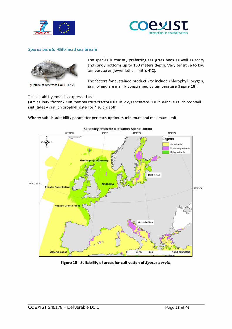
Sparus aurata -Gilt-head sea bream

The species is coastal, preferring sea grass beds as well as rocky and sandy bottoms up to 150 meters depth. Very sensitive to low temperatures (lower lethal limit is 4°C). The factors for sustained productivity include chlorophyll, oxygen, salinity and are mainly constrained by temperature (Figure 18).

The suitability model is expressed as: (sut_salinity*factor5+suit_temperature*factor10+suit_oxygen*factor5+suit_wind+suit_chlorophyll + suit_tides + suit_chlorophyll_satellite)* suit_depth Where: suit- is suitability parameter per each optimum minimum and maximum limit.

Figure 18 - Suitability of areas for cultivation of Sparus aurata.


Venerupis corrugata - Pullet carpet shell

The shell’s habitat is mainly on mixed sandy sediments starting from shallow zone of the lower shore to the shallow sub littoral. The species it’s a burrowing species and does not byssus. The distribution ranges from northern Norway to the Mediterranean and north-west Africa (Venerupis pullastra, Marine Species Identification Portal, 2012). This species is highly sensitive to a

decrease in water salinity from fresh water and rain. The factors for sustained productivity include temperature, chlorophyll and oxygen and are constrained by salinity (Figure 19). The suitability model is expressed as: (sut_salinity*factor10+suit_temperature*factor10+suit_oxygen*factor5+suit_wind+suit_chlorophyll + suit_tides + suit_chlorophyll_satellite)* suit_depth Where: suit- is suitability parameter per each optimum minimum and maximum limit.

Figure 19 - Suitability of areas for cultivation of Venerupis corrugata.


4. Conclusion and recommendations

The presented suitability maps show three levels of suitability: highly, moderately and not suitable. Highly suitable areas are areas where cultivation of a given species is possible, because the main environmental conditions are within the optimum range (between the minimum and maximum limits). In moderately suitable areas some factors are not within the species’ optimum levels, but only within its tolerable range. In these areas, a modification of environmental conditions, e.g. to provide higher chlorophyll concentration, increase water temperature and/or to ensure a sufficient supply of oxygen is needed. However, to select the applicable intervention instrument a more detailed analysis of limiting factors and natural conditions is required. The selection of optimum limits shows that many species, like Coregonus lavaretus, Crassostrea gigas, Ostrea edulis, Mytilus edulis, Mytilus galloprovincialis, Oncorhynchus mykiss, Salmo salar, Solea senegalensis, Sparus aurata, Pecten maximus,Crassostrea angulata and Gadus morhua are very sensitive to changes in the water temperature required for their optimal growth and reproduction. For instance, Solea senegalensis is a tropical species and therefore cultivation in European sites will be only possible in areas warm enough for the species to reproduce. The areas along the coast of the Aegean Sea, some areas in Mediterranean Sea and Bay of Biscay will be moderately suitable. However, as mentioned in the scientific literature, the cultivation of the Solea senegalensis in European waters has not been successful so far, because of the special feeding pattern and behaviour of the species, which is very difficult to reconstruct in non-native and artificial environments. Apart from the water temperature, salinity is proven to be another critical factor to consider in cultivating Coregonus lavaretus, Venerupis decussata, Venerupis corrugata and Gadus morhua. Coregonus lavaretus is a fresh water species and require waters with very low salinity, which can be found only in the Baltic Sea. In contrast, Venerupis decussata, Venerupis corrugata and Gadus morhua require high salinity marine waters to thrive. One of the main limiting critical factors is found to be in water depth, as the majority of the selected species prefer coastal and shallow waters as their habitat. The seabed sediment and substrate is important for Mytilus edulis, Mytilus galloprovincialis, Crassostrea angulata and Crassostrea gigas with a preference for mixed sediments. In addition to mixed sediments, some of the species require availability of hard substrate to form banks or reefs. The suitability modelling is not limited to produce suitability mapping only for European Seas. In future it is possible to extend the modelling with modification and adding more parameters and data into the constructed model. Current maps do not fully include the Northern part of the Norway, because of the boundary limits of the EUSea Map seabed habitat and bathymetry dataset (Figure 1). The choice to use selected datasets was based on the intension to have uniform datasets across all regions with certified and accepted accuracy and confidence levels, as well as from well-known and open sources. One special case in the suitability maps is specie of the Japanese Oyster. It is a native species in coastal areas of Japan and have been introduced in North Sea area more than once, including the Dutch Eastern Scheldt in since 1964 (Drinkwaard, 1999). The successful escape of the Japanese


Oyster to the wild from caged environment occurred in the Netherlands during 1975 and 1976. This was contrary to the expectations that it would not be capable of reproducing under the natural conditions in Dutch waters (Drinkwaard, 1999), where the specie was cultivated initially. After its initial escape the Japanese Oyster was allowed to establish itself thoroughly. This has left us with no feasible methods to eradicate the species, should we still want to. Hence as the suitability modelling is only considering only the optimum minimum and maximum limits for optimal growth of a species only from their based on its native environment. As a result the actual suitability maps for Japanese Oyster and as well as seabass within show that the North Sea are presented as moderately suitable, when where actually it both species is are widely spread and not uncommon. The GES 2 element of Marine Strategy Framework Directive stated to avoid new introductions of invasive species, and considering the case of Japanese Oyster it was introduced before the directive. The same is for Gadus morhua, Pecten maximum and Mytilus edulis in the Mediterranean Sea. We could state that it is a case in point that the presented suitability maps have limitations. Some of these limitations may stem from the quality of the data sets on physical and biological start as used to produce the maps. Other limitations come from insufficient knowledge on the true value of the requirements that each species places on its environment, e.g. for Crassostrea gigas the data that the literature review has brought to light still reflects a situation where the North Sea is only moderately suitable for this species, where we now know from observing its successful invasion that it can be very successful here. A success that may in part be due to the absence of its natural predators. The literature review revealed that existing scientific studies on optimum limits are not always complete and in some cases are even missing. In many cases the information on temperature, salinity and oxygen diverged across the different information sources. It is recommended to gain more knowledge on physical and biological requirements for cultivating these selected species, to be able to refine and to obtain more precise view. In addition, instead of using absolute values to represent optimum / tolerance limits, use could be made of modelled probability distributions. The main conclusion of the study is that suitability mapping is a useful tool in spatial planning and decision-making, showing the potential of culturing species at first glance. Further research is recommended to aid in defining parameters for suitability, including information on seasonal variation, and also to refine the ranges of optimal conditions for the culture of species, such as the sixteen that are presented in this study. This recommendation is largely based on our finding from the literature study which revealed that many limits are derived from experiments conducted in scientific conditions, which cannot truly represent natural nor aquaculture conditions. The resolution of data set used in suitability mapping is important in presenting the level of details to be shown in suitability maps. For general overview like it was in current project the resolution of 200 meters produced sufficient level of details to demonstrate the potential of culturing species at first glance. It is also advised not to use very high resolution data in such global overview maps, as it will cost storage space and computation time. To produce suitability maps for localised areas, it is recommended to use high resolution, e.g. better than 20 meters datasets, to be able to see the required particulars. For suitability modelling in the coastal zones high resolution data is required, to fetch local variations. One of such examples can be seen on suitability maps for the Blue mussel along the southern coast of Norway. The current


suitability maps show the low suitability, while experience from the industry have shown good growth conditions in these areas, although local variations might influence the suitability heavily. The adjustment of modelling parameters for coastal zones is recommended, to be able to match the modelling with industry experiences. Considering the preservation of the natural environment and taking into account the possible invasive character of a non-native species (e.g. the Japanese Oyster), it is recommended that non-native species are critically reviewed before attempting to aquaculture them in a new environment. Selecting a location where the natural conditions are at best, moderately suitable, and requiring human intervention to complete the reproductive cycle or even basic survival is the safest option. For aquaculture of species inside their native range it is recommended to choose highly suitable areas, and for artificial, caged cultivation, moderately suitable areas are expected to be commercially and economically feasible.


References

1. Alfaro, A. C. and A. G. Jeffs, 2003, "Variability in mussel settlement on suspended ropes

placed at Ahipara Bay, Northland, New Zealand." Aquaculture 216(1–4): 115-126. 2. G. P. Arnold and M. Greer Walker, “Vertical movements of cod (Gadus morhua L.) in the

open sea and the hydrostatic function of the swim bladder”. ICES J. Mar. Sci. (1992) 49(3): 357-372 doi:10.

3. M. Albentosa and J. Moyano, 2007, “Differences in the digestive biochemistry between the intertidal clam, Ruditapes decussatus, and the sub tidal clam, Venerupis pullastra”. Aquaculture International (2009) 17:273–282.

4. Batista, Frederico M., et al, 2008, “Comparative study of shell shape and muscle scar pigmentation in the closely related cupped oysters Crassostrea angulata, C. gigas and their reciprocal hybrids”. Aquatic Living Resources 21.1 (2008): 31-38.

5. Bell, J. D., 1983, “Effects of Depth and Marine Reserve Fishing Restrictions on the Structure of a Rocky Reef Fish Assemblage in the North-Western Mediterranean Sea.” Journal of Applied Ecology 20(2): 357-369.

5. Björn Björnsson, Agnar Steinarsson, and Matthías Oddgeirsson, 2001, “Optimal temperature for growth and feed conversion of immature cod (Gadus morhua L.)”. ICES J. Mar. Sci. (2001) 58(1): 29-38 doi:10.1006/jmsc.2000.0986 .

6. Burrows MT, Harvey R, Robb L, 2008, “Wave exposure indices from digital coastlines and the prediction of rocky shore community structure”. Marine Ecology Progress. Series, 353:1–12.

7. Burt, K., D. Hamoutene, et al, 2012, "Environmental conditions and occurrence of hypoxia within production cages of Atlantic salmon on the south coast of Newfoundland." Aquaculture Research 43(4): 607-620.

8. Bombace et al, 2000, “Artificial reefs in the Adriatic Sea”. Pages 31-63 in Jensen A.C., K.J. Collins, Lockwood A.P.M. (eds.) “Artificial reefs in European Seas” Kluwer Academic Publishers.

9. Cheng, W., C.-H. Li, et al, 2004, "Effect of dissolved oxygen on the immune response of Haliotis diversicolor supertexta and its susceptibility to Vibrio parahaemolyticus." Aquaculture 232(1–4): 103-115.

10. Comeau, L. A., R. Sonier, et al, 2010, "A novel approach to measuring chlorophyll uptake by cultivated oysters." Aquaculture Engineering 43(2): 71-77.

11. Christophersen, G. and Ø. Strand, 2003, "Effect of reduced salinity on the great scallop (Pecten maximus) spat at two rearing temperatures." Aquaculture 215(1–4): 79-92.

12. Chelsey E. Lumb and Timothy B. Johnson, 2012, “Retrospective growth analysis of lake whitefish (Coregonus clupeaformis) in Lakes Erie and Ontario”, 1954–2003. Advanced Limnology, 63, p. 429–454. Biology and Management of Coregonid Fishes – 2008.

13. Dag Klaveness, 1990, “Size Structure and Potential Food Value of the Plankton Community to Ostrea edulis L. in a Traditional Norwegian “Osterspoll”, Aquaculture, 66 (1990) 231-247 231, Elsevier Science Publishers B.V., Amsterdam - Printed in the Netherlands.

14. Desoutter, M.,In J.C. Quero, J.C. Hureau, C. Karrer, A. Post and L. Saldanha (eds.), 1990,“Check-list of the fishes of the eastern tropical Atlantic (CLOFETA)”. JNICT, Lisbon; SEI, Paris; and UNESCO, Paris. Vol. 2.


15. Divanach, P., N. Papandroulakis, et al, 1997, "Effect of water currents on the development of skeletal deformities in sea bass (Dicentrarchus labrax L.) with functional swimbladder during post larval and nursery phase." Aquaculture 156(1–2): 145-155.

16. T Dempster, P Sanchez-Jerez, JT Bayle-Sempere, F Giménez-Casalduero, C Valle, 2011, “Attraction of wild fish to sea-cage fish farms in the south-western Mediterranean Sea: spatial and short-term temporal variability”. Marine Ecology Progress Series 242, 237-252, 2011.

17. Denis Lionel, Elizabeth Alliot and Daniel Grzebyk, 1999, Clearance rate responses of Mediterranean mussels, Mytilus galloprovincialis, to variations in the flow, water temperature, food quality and quantity. Aquatic Living Resources, 12, pp. 279-288 doi: 10.1016/S0990-7440(00)86639-5.

18. Dadswell, M. J., A. D. Spares, et al,2010, "The North Atlantic subpolar gyre and the marine migration of Atlantic salmon Salmo salar: the ‘Merry-Go-Round’ hypothesis." Journal of Fish Biology 77(3): 435-467.

19. Diederich S,2006, “High survival and growth rates of introduced Pacific oysters may cause restrictions on habitat use by native mussels in the Wadden Sea”. Journal of Experimental Marine Biology and Ecology 328(2):211-227.

20. Effects of temperature and salinity on comparative embryo development and mortality of Atlantic cod (Gadus morhua L.) and haddock (Melanogrammus aeglefinus (L.)),Conseil permanent international pour l'exploration, 1976, 36(3): 220-228.

21. Fabi G. and Fiorentini L., 1990. “Shellfish culture associated with artificial reefs”. FAO Fish. Rep.428: 99-107).

22. R. R. C. Edwards, D. M. Finlayson and J. H. Steele, Jr. 1972, “An Experimental Study of the oxygen consumption, growth, and metabolism of the Cod (Gadus Morhua L.),”, Vol. 8, pp. 299-309; North-Holland Publishing Company.

23. FAO, 2012, Fisheries and Aquaculture Department, http://www.fao.org/fi/website/MultiQueryAction.do?

24. FAO, 2005-2012, Cultured Aquatic Species Information Programme. Oncorhynchus mykiss. Cultured Aquatic Species Information Programme . Text by Cowx, I. G. In: FAO Fisheries and Aquaculture Department [online]. Rome. Updated 15 June 2005. http://www.fao.org/fishery/culturedspecies/Oncorhynchus_mykiss/en.

25. Fisheries Research Report NO. 130, 2001, Environmental requirements and tolerances of Rainbow trout (Oncorhynchus mykiss) and Brown trout (Salmo trutta) with special reference to Western Australia: A review. Brett Molony, Fisheries Research Division WA Marine Research Laboratories PO Box 20 North Beach Western Australia 6920.

26. Fredriksson, D. W., M. R. Swift, et al, 2003, “Fish cage and mooring system dynamics using physical and numerical models with field measurements.” Aquaculture Engineering 27(2): 117-146..1093/icesjms/49.3.357.

27. Fotel, F. L., N. J. Jensen, et al, 1999, "In situ and laboratory growth by a population of blue mussel larvae (Mytilus edulis L.) from a Danish embayment, Knebel Vig." Journal of Experimental Marine Biology and Ecology 233(2): 213-230.

28. Filgueira, R., J. Grant, et al, 2010, "A simulation model of carrying capacity for mussel culture in a Norwegian fjord: Role of induced upwelling." Aquaculture 308(1–2): 20-27.

29. Guerreiro, I., H. Peres, et al, 2012, "Effect of temperature and dietary protein/lipid ratio on growth performance and nutrient utilization of juvenile Senegalese sole (Solea senegalensis)." Aquaculture Nutrition 18(1): 98-106.

http://www.fao.org/fi/website/MultiQueryAction.do

http://www.fao.org/fishery/culturedspecies/Oncorhynchus_mykiss/en


30. Glamuzina, B., J. Jug-Dujaković, et al, 1989, "Preliminary studies on reproduction and larval rearing of common dentex, Dentex dentex (Linnaeus 1758)." Aquaculture 77(1): 75-84.

31. Hanson, J. M., W. C. Mackay, et al, 1988, "The effects of water depth and density on the growth of a unionid clam*." Freshwater Biology 19(3): 345-355.

32. Han, K., S. Lee, et al, 2008, "The effect of temperature on the energy budget of the Manila clam." Aquaculture International 16(2): 143-152.

33. Heral M., 1989, “Traditional oyster culture in France”. Pages 342-387 in G. Barnabé, J.F. Solbé and L. Laird, editors. Aquaculture Volume 1. Ellis Horwood London, pp 342-387.

34. Imsland, A.K. and Jonassen, T.M. 2001, “Regulation of growth in turbot (Scophthalmus maximus Rafinesque) and Atlantic halibut (Hippoglossus hippoglossus L.): aspects of environment genotype interactions”. Rev. Fish Biol. Fisheries. 11, 71–90.

35. Imsland, A.K., Foss, A., Conceição, L.E.C., Dinis, M.T., Delbare, D., Schram, E., Kamstra, A., Rema, P., White, P., 2003, “A review of the culture potential of Solea solea and S. senegalensis”. Rev. Fish Biol. Fish. 13, 379–407.

36. J.Y. Jouvenel, D.A. Pollard,2001, “Some effects of marine reserve protection on the population structure of two spear fishing target-fish species, Dicentrarchus labrax (Moronidae) and Sparus aurata (Sparidae), in shallow inshore waters, along a rocky coast in the north-western Mediterranean Sea”. Aquatic Conservation: Marine and Freshwater Ecosystems, 11 (2001), pp. 1–9.

37. Kautsky, N.,1982, "Growth and size structure in a Baltic Mytilus edulis population." Marine Biology 68(2): 117-133.

38. Kythera Natural History Museum, Germany - http://www.kytherafamily.net/index.php?nav=87-102&cid=170&did=579&pageflip=2.

39. Lambert, Y. and J.-D. Dutil, 2001, "Food intake and growth of adult Atlantic cod (Gadus morhua L.) reared under different conditions of stocking density, feeding frequency and size-grading." Aquaculture 192(2–4).

40. Lambert, Y., J.-D. Dutil, et al, 1994, "Effects of Intermediate and Low Salinity Conditions on Growth Rate and Food Conversion of Atlantic Cod (Gadus morhua)." Canadian Journal of Fisheries and Aquatic Sciences 51(7): 1569-1576.

41. Laurence, G. C., and A. C. Rogers, 1976,” Effects of temperature and salinity on comparative embryo development and mortality of Atlantic cod (Gadus morhua L.) and haddock (Melanogrammus aeglefinus L.)”. Journal du Conseil, Conseil International pour l’Exploration de la Mer 36:220–228.

42. Laing, I., 2000, "Effect of temperature and ration on growth and condition of king scallop (Pecten maximus) spat." Aquaculture 183(3–4): 325-334.

43. Lam, K. and B. Morton, 2003, "Mitochondrial DNA and morphological identification of a new species of Crassostrea (Bivalvia: Ostreidae) cultured for centuries in the Pearl River Delta, Hong Kong, China." Aquaculture 228(1–4): 1-13.

44. Lundsgaard-Hansen, B., B. Matthews, et al, 2013, "Adaptive plasticity and genetic divergence in feeding efficiency during parallel adaptive radiation of whitefish (Coregonus spp.)." Journal of Evolutionary Biology 26(3): 483-498.

45. The Marine Species Identification Portal, 2012, ETI Bioinformatics, the Netherlands. http://species-identification.org/index.php.

46. John Merriner, 2004, “Anadromous Fishes of the Potomac estuary”, Pub157, 2004, Sailing Directions (Enroute) - Korea and China (10th Edition) by N.I.M.A. (Jan 1, 2004)

47. Maine Department of Inland Fisheries and Wildlife, 2010, http://www.maine.gov/ifw/contactus.htm.

http://www.kytherafamily.net/index.php?nav=87-102&cid=170&did=579&pageflip=2

http://www.maine.gov/ifw/contactus.htm


48. MacDonald and Thompson, 1986, “Influence of temperature and food availability on the ecological energetics of the giant scallop Placopecten magellanicus”. III Physiological ecology, the gametogenic cycle and scope for growth, Mar. Biol., 93 (1986), pp. 37–48.

49. MartÍNez-Llorens, S., A. N. A. T. Vidal, et al,2009, "Optimum dietary soybean meal level for maximizing growth and nutrient utilization of on-growing gilthead sea bream (Sparus aurata)." Aquaculture Nutrition 15(3): 320-328.

50. Murre Techniek B.V., 2012, http://www.murre.nl/nederlands/nieuws.asp. 51. Norton-Griffith, M., 1967, "Some ecological aspects of the feeding behaviour of the

oystercatcher haematopus ostralegus on the edible mussel mytilus edulis." Ibis 109(3): 412-424.

52. Nicolas, D., F. Le Loc'h, et al, 2007, "Relationships between benthic macro fauna and habitat suitability for juvenile common sole (Solea solea, L.) in the Vilaine estuary (Bay of Biscay, France) nursery ground." Estuarine, Coastal and Shelf Science 73(3–4): 639-650.

53. Papoutsoglou, S. E., N. Karakatsouli, et al, 2006, "Effects of rearing density on growth, brain neurotransmitters and liver fatty acid composition of juvenile white sea bream Diplodus sargus L." Aquaculture Research 37(1): 87-95.

54. Pogoda, B., B. H. Buck, et al,2011, "Growth performance and condition of oysters (Crassostrea gigas and Ostrea edulis) farmed in an offshore environment (North Sea, Germany)." Aquaculture 319(3–4): 484-492. Jouvenel and Pollard, 2001.

55. Poppe, G. T. and Goto, Y, 1991, “European seashells". Vol 1 (Polyplacophora, Caudofoveata, Solenogastra, Gastropoda)”.Verlag Christa Hemmen.

56. Roberts, C. M. and N. V. C. Polunin, 1991, "Are marine reserves effective in management of reef fisheries?". Reviews in Fish Biology and Fisheries 1(1): 65-91.

57. Rhody, N. R., N. A. Nassif, et al, 2010, "Effects of salinity on growth and survival of common snook Centropomus undecimalis (Bloch, 1792) larvae." Aquaculture Research 41(9): e357-e360.

58. SÁ, R., P. PousÃO-Ferreira, et al, 2008, "Dietary protein requirement of white sea bream (Diplodus sargus) juveniles." Aquaculture nutrition. 14(4): 309-317.

59. L. Sofronios E Papoutsoglou, Nafsika Karakatsouli, Gianluka Pizzonia, Christina Dalla, Alexia Polissidis and Zeta Papadopoulou-Daifoti, 2006, “Effects of rearing density on growth, brain neurotransmitters and liver fatty acid composition of juvenile white sea bream Diplodus sargus”. Aquaculture Research, 2006.

60. Schurmann, H. and J. F. Steffensen, 1992, "Lethal oxygen levels at different temperatures and the preferred temperature during hypoxia of the Atlantic cod, Gadus morhua L." Journal of Fish Biology 41(6): 927-934.

61. S2494 - Coregonus lavaretus – Whitefish, 2006, European Community Directive on the Conservation of Natural Habitats and of Wild Fauna and Flora. http://jncc.defra.gov.uk/pdf/Article17/FCS2007-S2494-Final.pdf.

62. Thorarinsdóttir, G. G., 1991, "The Iceland scallop, Chlamys islandica (O.F. Müller) in Breidafjördur, west Iceland. I. Spat collection and growth during the first year." Aquaculture 97(1): 13-23.

63. Vinagre, C., T. Ferreira, et al, 2009, "Latitudinal gradients in growth and spawning of sea bass, Dicentrarchus labrax, and their relationship with temperature and photoperiod." Estuarine, Coastal and Shelf Science 81(3): 375-380.

64. Vinagre, C., V. Fonseca, et al,2008, "Habitat specific growth rates and condition indices for the sympatric soles Solea solea (Linnaeus, 1758) and Solea senegalensis Kaup 1858, in the

http://www.murre.nl/nederlands/nieuws.asp

http://jncc.defra.gov.uk/pdf/Article17/FCS2007-S2494-Final.pdf


Tagus estuary, Portugal, based on otolith daily increments and RNA-DNA ratio." Journal of Applied Ichthyology 24(2): 163-169.

65. Vielma, J., T. Mäkinen, et al, 2000, "Influence of dietary soy and phytase levels on performance and body composition of large rainbow trout (Oncorhynchus mykiss) and algal availability of phosphorus load." Aquaculture 183(3–4): 349-362.

66. Widdows, J., P. Fieth, et al, 1979, "Relationships between sextons, available food and feeding activity in the common mussel Mytilus edulis." Marine Biology 50(3): 195-207.

67. Wheeler, A., 1992, “A list of the common and scientific names of fishes of the British Isles”. J. Fish Biol. 41(1):1-37.

68. Whitefish, Nature gate, http://www.luontoportti.com/suomi/en/kalat/whitefish. 69. Wolff WJ, Reise K.,2002, “Oyster imports as a vector for the introduction of alien species into

northern and western European coastal waters”. In: Leppäkoski E, Gollasch S, Olenin S (eds) Invasive aquatic species of Europe: Distribution, Impact and Management Kluwer, Dordrecht, the Netherlands, pp. 193-205.

70. Whitehead, PJP; Bauchot, ML; Hureau, JC; Nielsen, J.; Tortonese, E., (Eds), 1984,”Fishes of the north-eastern Atlantic and the Mediterranean”, Vols. 1, 2 and 3. UNESCO, Paris, ISBN 92- 3-002215-2

http://www.luontoportti.com/suomi/en/kalat/whitefish


Annex I: Chlorophyll image MODIS TERRA satellite

Satellite image from MODIS TERRA satellite (USA) presenting seasonal changes in chlorophyll during spring 2012.


Annex II: Ocean salinity SMOS satellite

Salinity data measured by SMOS satellite on July 12, 2012: The low salinity areas also include areas not measured, because of satellite resolution in 200 km and absence of data for validation.


Annex III: The suitability model- Model Builder ArcGIS


Annex IV: Example of python script for Coregonus lavaretus

# --------------------------------------------------------------------------- # coregonus_script.py # Created on: 2013-02-25 15:06:50.00000 # (generated by ArcGIS/ModelBuilder) # Description: # The suitability maps presenting areas which are: # - Highly suitable for aquaculture of Coregonus lavaretus # - Moderately suitable and # - Not suitable # # --------------------------------------------------------------------------- # Import arcpy module import arcpy # Check out any necessary licenses arcpy.CheckOutExtension("spatial") # Set Geoprocessing environments arcpy.env.snapRaster = "" arcpy.env.extent = "-40.2714490671601 21.728054596105 81.9356394184109 76.999999572" arcpy.env.cellSize = "G:\\Co_exist\\Model suitability\\Data\\north_sea1.tif" # Local variables: west_mediterrain1_tif = "G:\\Co_exist\\Model suitability\\Data\\west_mediterrain1.tif" north_sea1_tif = "G:\\Co_exist\\Model suitability\\Data\\north_sea1.tif" celtic1_tif = "G:\\Co_exist\\Model suitability\\Data\\celtic1.tif" bay_biscay1_tif = "G:\\Co_exist\\Model suitability\\Data\\bay_biscay1.tif" baltic_tif = "G:\\Co_exist\\Model suitability\\Data\\baltic.tif" aegean-Lev1_tif = "G:\\Co_exist\\Model suitability\\Data\\aegean-Lev1.tif" adriatic_med1_tif = "G:\\Co_exist\\Model suitability\\Data\\adriatic.med1.tif" Coregonus_lavaretus = "G:\\Co_exist\\Model suitability\\Coregonus lavaretus" chr_eu_20121 = "chr_eu_20121" seabed_habitat_baltic_shp = "G:\\Co_exist\\Model suitability\\Data\\seabed_habitat_baltic.shp" seabed_habitat_celtic_north_sea_shp = "G:\\Co_exist\\Model suitability\\Data\\seabed_habitat_celtic_north_sea.shp" seabed_habitat_west_med_shp = "G:\\Co_exist\\Model suitability\\Data\\seabed_habitat_west_med.shp" ocean_data_nasa = "ocean_data_nasa" eu_seas__2_ = "eu_seas" cor_sal2 = "G:\\Co_exist\\Model suitability\\Coregonus lavaretus_suit\\cor_sal2" cor_balt = "G:\\Co_exist\\Model suitability\\Coregonus lavaretus\\cor_balt"


cor_north = "G:\\Co_exist\\Model suitability\\Coregonus lavaretus\\cor_north" cor_celtic = "G:\\Co_exist\\Model suitability\\Coregonus lavaretus\\cor_celtic" cor_biscay = "G:\\Co_exist\\Model suitability\\Coregonus lavaretus\\cor_biscay" cor_med = "G:\\Co_exist\\Model suitability\\Coregonus lavaretus\\cor_med" cor_aeg = "G:\\Co_exist\\Model suitability\\Coregonus lavaretus\\cor_aeg" cor_adr = "G:\\Co_exist\\Model suitability\\Coregonus lavaretus\\cor_adr" cor_temp2 = "G:\\Co_exist\\Model suitability\\Coregonus lavaretus_suit\\cor_temp2" cor_wind2 = "G:\\Co_exist\\Model suitability\\Coregonus lavaretus_suit\\cor_wind2" cor_chr2 = "G:\\Co_exist\\Model suitability\\Coregonus lavaretus_suit\\cor_chr2" cor_tides2 = "G:\\Co_exist\\Model suitability\\Coregonus lavaretus_suit\\cor_tides2" cor_oxygen2 = "G:\\Co_exist\\Model suitability\\Coregonus lavaretus_suit\\cor_oxygen2" cor_chr_sat1 = "G:\\Co_exist\\Model suitability\\Coregonus lavaretus\\cor_chr_sat1" balt_sed = "G:\\Co_exist\\Model suitability\\Coregonus lavaretus_suit\\balt_sed" balt_sal = "G:\\Co_exist\\Model suitability\\Coregonus lavaretus_suit\\balt_sal" balt_bio = "G:\\Co_exist\\Model suitability\\Coregonus lavaretus_suit\\balt_bio" celt_sed = "G:\\Co_exist\\Model suitability\\Coregonus lavaretus_suit\\celt_sed" celt_bio = "G:\\Co_exist\\Model suitability\\Coregonus lavaretus_suit\\celt_bio" med_sed = "G:\\Co_exist\\Model suitability\\Coregonus lavaretus_suit\\med_sed" med_bio = "G:\\Co_exist\\Model suitability\\Coregonus lavaretus_suit\\med_bio" balt_sed1 = "G:\\Co_exist\\Model suitability\\Coregonus lavaretus_suit\\balt_sed1" balt_sal1 = "G:\\Co_exist\\Model suitability\\Coregonus lavaretus_suit\\balt_sal1" balt_bio1 = "G:\\Co_exist\\Model suitability\\Coregonus lavaretus_suit\\balt_bio1" celt_sed1 = "G:\\Co_exist\\Model suitability\\Coregonus lavaretus_suit\\celt_sed1" celt_bio1 = "G:\\Co_exist\\Model suitability\\Coregonus lavaretus_suit\\celt_bio1" med_sed1 = "G:\\Co_exist\\Model suitability\\Coregonus lavaretus_suit\\med_sed1" med_bio1 = "G:\\Co_exist\\Model suitability\\Coregonus lavaretus_suit\\med_bio1" sal_suit3 = "G:\\Co_exist\\Model suitability\\Coregonus lavaretus_suit\\sal_suit3" temp_suit3 = "G:\\Co_exist\\Model suitability\\Coregonus lavaretus_suit\\temp_suit3" wind_suit3 = "G:\\Co_exist\\Model suitability\\Coregonus lavaretus_suit\\wind_suit3" chr_suit3 = "G:\\Co_exist\\Model suitability\\Coregonus lavaretus_suit\\chr_suit3" tides_suit3 = "G:\\Co_exist\\Model suitability\\Coregonus lavaretus_suit\\tides_suit3" oxygen_suit3 = "G:\\Co_exist\\Model suitability\\Coregonus lavaretus_suit\\oxygen_suit3" suitable1 = "G:\\Co_exist\\Model suitability\\Coregonus lavaretus_suit\\suitable1" corcr_st1sub1 = "G:\\Co_exist\\Model suitability\\Coregonus lavaretus_suit\\corcr_st1sub1" balt_sed3 = "G:\\Co_exist\\Model suitability\\Coregonus lavaretus_suit\\balt_sed3" balt_sal3 = "G:\\Co_exist\\Model suitability\\Coregonus lavaretus_suit\\balt_sal3" balt_bio3 = "G:\\Co_exist\\Model suitability\\Coregonus lavaretus_suit\\balt_bio3" celt_sed3 = "G:\\Co_exist\\Model suitability\\Coregonus lavaretus_suit\\celt_sed3" celt_bio3 = "G:\\Co_exist\\Model suitability\\Coregonus lavaretus_suit\\celt_bio3" med_sed3 = "G:\\Co_exist\\Model suitability\\Coregonus lavaretus_suit\\med_sed3" med_bio3 = "G:\\Co_exist\\Model suitability\\Coregonus lavaretus_suit\\med_bio3" suit_class = "G:\\Co_exist\\Model suitability\\Coregonus lavaretus\\suit_class" # Process: Polygon to Raster (7) arcpy.PolygonToRaster_conversion(seabed_habitat_baltic_shp, "substrate", balt_sed, "CELL_CENTER", "NONE", north_sea1_tif) # Process: Reclassify (14)


arcpy.gp.Reclassify_sa(balt_sed, "SUBSTRATE", "'Mud to sandy mud' 0;'Sand to muddy sand' 1;'Coarse sediment' 2;'Mixed sediment' 3;Till 4;'Rock or other hard substrata' 5;' ' 6", balt_sed1, "NODATA") # Process: Extract by Mask (3) arcpy.gp.ExtractByMask_sa(balt_sed1, eu_seas__2_, balt_sed3) # Process: Polygon to Raster (8) arcpy.PolygonToRaster_conversion(seabed_habitat_baltic_shp, "Salinity", balt_sal, "CELL_CENTER", "NONE", north_sea1_tif) # Process: Reclassify (15) arcpy.gp.Reclassify_sa(balt_sal, "SALINITY", "Oligohaline 1;'Mesohaline I' 0;'Mesohaline II' 0;'Mesohaline III' 0;Polyhaline 0;'Fully marine' 0;Mesohaline 0", balt_sal1, "NODATA") # Process: Extract by Mask (4) arcpy.gp.ExtractByMask_sa(balt_sal1, eu_seas__2_, balt_sal3) # Process: Polygon to Raster (9) arcpy.PolygonToRaster_conversion(seabed_habitat_baltic_shp, "BioZgroup", balt_bio, "CELL_CENTER", "NONE", north_sea1_tif) # Process: Reclassify (16) arcpy.gp.Reclassify_sa(balt_bio, "BIOZGROUP", "Shallow 1;'Shallow photic' 1;'Shallow aphotic' 1;Shelf 0", balt_bio1, "NODATA") # Process: Extract by Mask (5) arcpy.gp.ExtractByMask_sa(balt_bio1, eu_seas__2_, balt_bio3) # Process: Polygon to Raster (10) arcpy.PolygonToRaster_conversion(seabed_habitat_celtic_north_sea_shp, "substrate", celt_sed, "CELL_CENTER", "NONE", north_sea1_tif) # Process: Reclassify (17) arcpy.gp.Reclassify_sa(celt_sed, "SUBSTRATE", "Seabed 0;'Mud to sandy mud' 0;'Sand to muddy sand' 0;'Coarse sediment' 1;'Mixed sediment' 1;Till 1;'Rock or other hard substrata' 1", celt_sed1, "NODATA") # Process: Extract by Mask (6) arcpy.gp.ExtractByMask_sa(celt_sed1, eu_seas__2_, celt_sed3) # Process: Polygon to Raster (11) arcpy.PolygonToRaster_conversion(seabed_habitat_celtic_north_sea_shp, "BioZgroup", celt_bio, "CELL_CENTER", "NONE", north_sea1_tif) # Process: Reclassify (18) arcpy.gp.Reclassify_sa(celt_bio, "BIOZGROUP", "Shallow 1;'Shallow photic' 1;'Shallow aphotic' 1;Shelf 1;Bathyal 0;Abyssal 0", celt_bio1, "NODATA")


# Process: Extract by Mask (7) arcpy.gp.ExtractByMask_sa(celt_bio1, eu_seas__2_, celt_bio3) # Process: Polygon to Raster (12) arcpy.PolygonToRaster_conversion(seabed_habitat_west_med_shp, "substrate", med_sed, "CELL_CENTER", "NONE", north_sea1_tif) # Process: Reclassify (19) arcpy.gp.Reclassify_sa(med_sed, "SUBSTRATE", "'Rock or other hard substrata' 1;'Coarse and mixed sediment' 1;Sand 0;'Sandy mud' 0;'Muddy sand' 0;Mud 0;'Posidonia oceanica' 0;'Cymodocea nodosa' 0", med_sed1, "NODATA") # Process: Extract by Mask (8) arcpy.gp.ExtractByMask_sa(med_sed1, eu_seas__2_, med_sed3) # Process: Polygon to Raster (13) arcpy.PolygonToRaster_conversion(seabed_habitat_west_med_shp, "BioZgroup", med_bio, "CELL_CENTER", "NONE", north_sea1_tif) # Process: Reclassify (20) arcpy.gp.Reclassify_sa(med_bio, "BIOZGROUP", "'Shallow photic' 1;Shallow 1;'Shallow aphotic' 1;Shelf 1;Bathyal 0;Abyssal 0", med_bio1, "NODATA") # Process: Extract by Mask (9) arcpy.gp.ExtractByMask_sa(med_bio1, eu_seas__2_, med_bio3) # Process: Polygon to Raster arcpy.PolygonToRaster_conversion(ocean_data_nasa, "SALINITY_M", cor_sal2, "CELL_CENTER", "NONE", north_sea1_tif) # Process: Reclassify arcpy.gp.Reclassify_sa(cor_sal2, "Value", sal_suit3, "NODATA") # Process: Polygon to Raster (2) arcpy.PolygonToRaster_conversion(ocean_data_nasa, "SST_MIN_MO", cor_temp2, "CELL_CENTER", "NONE", north_sea1_tif) # Process: Reclassify (9) arcpy.gp.Reclassify_sa(cor_temp2, "Value", temp_suit3, "NODATA") # Process: Polygon to Raster (6) arcpy.PolygonToRaster_conversion(ocean_data_nasa, "O2DISS_WOA", cor_oxygen2, "CELL_CENTER", "NONE", north_sea1_tif) # Process: Reclassify (22) arcpy.gp.Reclassify_sa(cor_oxygen2, "Value", oxygen_suit3, "NODATA")


# Process: Polygon to Raster (4) arcpy.PolygonToRaster_conversion(ocean_data_nasa, "CHLORA_S_4", cor_chr2, "CELL_CENTER", "NONE", north_sea1_tif) # Process: Reclassify (11) arcpy.gp.Reclassify_sa(cor_chr2, "Value", chr_suit3, "NODATA") # Process: Polygon to Raster (3) arcpy.PolygonToRaster_conversion(ocean_data_nasa, "WINDSPEED_", cor_wind2, "CELL_CENTER", "NONE", north_sea1_tif) # Process: Reclassify (10) arcpy.gp.Reclassify_sa(cor_wind2, "Value", wind_suit3, "DATA") # Process: Polygon to Raster (5) arcpy.PolygonToRaster_conversion(ocean_data_nasa, "TIDES_AVG_", cor_tides2, "CELL_CENTER", "NONE", north_sea1_tif) # Process: Reclassify (12) arcpy.gp.Reclassify_sa(cor_tides2, "Value", tides_suit3, "NODATA") # Process: Reclassify (13) arcpy.gp.Reclassify_sa(chr_eu_20121, "VALUE", ", cor_chr_sat1, "NODATA") # Process: Extract by Mask arcpy.gp.ExtractByMask_sa(cor_chr_sat1, eu_seas__2_, corcr_st1sub1) # Process: Reclassify (2) arcpy.gp.Reclassify_sa(baltic_tif, "VALUE", "-25 0 0;0 100 1", cor_balt, "NODATA") # Process: Reclassify (3) arcpy.gp.Reclassify_sa(north_sea1_tif, "Value", "-1531 -1014 0;-1014 -708 0;-708 -475 0;-475 -320 0;-320 -190 0;-190 -100 0;-100 0 1;0 33 0;33 780 0", cor_north, "NODATA") # Process: Reclassify (4) arcpy.gp.Reclassify_sa(celtic1_tif, "Value", cor_celtic, "NODATA") # Process: Reclassify (5) arcpy.gp.Reclassify_sa(bay_biscay1_tif, "Value", cor_biscay, "NODATA") # Process: Reclassify (6) arcpy.gp.Reclassify_sa(west_mediterrain1_tif, "Value", cor_med, "NODATA") # Process: Reclassify (7) arcpy.gp.Reclassify_sa(aegean-Lev1_tif, "Value", cor_aeg, "NODATA") # Process: Reclassify (8) arcpy.gp.Reclassify_sa(adriatic_med1_tif, cor_adr, "NODATA")


# Process: Mosaic To New Raster arcpy.MosaicToNewRaster_management("'G:\\Co_exist\\Model suitability\\Coregonus lavaretus\\cor_balt';'G:\\Co_exist\\Model suitability\\Coregonus lavaretus\\cor_north';'G:\\Co_exist\\Model suitability\\Coregonus lavaretus\\cor_celtic';'G:\\Co_exist\\Model suitability\\Coregonus lavaretus\\cor_biscay';'G:\\Co_exist\\Model suitability\\Coregonus lavaretus\\cor_med';'G:\\Co_exist\\Model suitability\\Coregonus lavaretus\\cor_aeg';'G:\\Co_exist\\Model suitability\\Coregonus lavaretus\\cor_adr'", Coregonus_lavaretus, "cor_depth.tif", "GEOGCS['GCS_ETRS_1989',DATUM['D_ETRS_1989',SPHEROID['GRS_1980',6378137.0,298.257222101]],PRIMEM['Greenwich',0.0],UNIT['Degree',0.0174532925199433]]", "8_BIT_UNSIGNED", "", "1", "LAST", "FIRST") # Process: Raster Calculator arcpy.gp.RasterCalculator_sa("(\"%sal_suit3%\" * 10 + \"%temp_suit3%\" * 10 + \"%oxygen_suit3%\" * 5 + \"%chr_suit3%\" + \"%wind_suit3%\" + \"%tides_suit3%\" + \"%corcr_st1sub1%\") * \"%cor_depth.tif%\" ", suitable1) # Process: Reclassify (21) arcpy.gp.Reclassify_sa(suitable1, "VALUE", "0 1 1;1 4 1;4 7 2;7 8 2;8 10 2;11 14 3;14 16 3;16 18 3;18 21 3", suit_class, "DATA")

Documents

COEXIST - WUR