Coherent Probes of Strong Field AtomicDynamics

A Thesis Presented

by

Uvo Christoph Holscher

to

The Graduate School

in Partial Fulfillment of the Requirements

for the Degree of

Master of Arts

in

Physics

Stony Brook University

August 2008

Stony Brook University

The Graduate School

Uvo Christoph Holscher

We, the Thesis committee for the above candidate for the Master of Artsdegree, hereby recommend acceptance of the Thesis.

Thomas C. Weinacht, Thesis Advisor

Assistant Professor, Department of Physics and Astronomy

Thomas H. Bergeman, Chairperson of Defense

Adjunct Professor, Department of Physics and Astronomy

Axel K. Drees

Professor, Department of Physics and Astronomy

Harold J. Metcalf

Professor, Department of Physics and Astronomy

This Thesis is accepted by the Graduate School.

Lawrence Martin

Dean of the Graduate School

ii

Abstract of the Thesis

Coherent Probes of Strong Field AtomicDynamics

by

Uvo Christoph Holscher

Master of Arts

in

Physics

Stony Brook University

2008

The work presented in this thesis studies the effect of ultrafast electromagnet-ically induced transparency (EIT) in a time domain picture. We demonstratethat ultrafast EIT is not only a version of CW laser EIT experiments scaledin time and field strength but shows a new dynamic. Time dependent Rabifrequencies of the light fields in conjunction with a short interaction time causea suppression of absorption at the transition frequency and a redistribution oflight among the spectrum.

A second experiment in the thesis discusses excitation mechanisms likeadiabatic rapid passage (ARP) for a four level system. We demonstrate astrong chirp dependence of the excitation paths and explain the behavior inthe dressed states picture. The preparation of the system leads to a collectiveemission of excited atoms called superfluorescence. We study the phenomenonand measure its characteristics.

iii

To Julia and my Family

Contents

List of Figures . . . . . . . . . . . . . . . . . . . . . . . . . . . . viii

List of Tables . . . . . . . . . . . . . . . . . . . . . . . . . . . . . ix

Acknowledgements . . . . . . . . . . . . . . . . . . . . . . . . . . x

1 Introduction . . . . . . . . . . . . . . . . . . . . . . . . . . . . . . 1

2 Experimental Setup . . . . . . . . . . . . . . . . . . . . . . . . . . 42.1 Pulse Generation . . . . . . . . . . . . . . . . . . . . . . . . . 42.2 Pulse Shaping . . . . . . . . . . . . . . . . . . . . . . . . . . . 62.3 Pulse Characterization . . . . . . . . . . . . . . . . . . . . . . 8

3 Configuration and Calibration of the GRENOUILLE . . . . . . . 93.1 Chirped Pulses . . . . . . . . . . . . . . . . . . . . . . . . . . 93.2 Pulse Characterization Background . . . . . . . . . . . . . . . 123.3 Design of the GRENOUILLE . . . . . . . . . . . . . . . . . . 143.4 Calibration of the GRENOUILLE . . . . . . . . . . . . . . . . 17

4 Theoretical Background . . . . . . . . . . . . . . . . . . . . . . . 254.1 Two-Level-Atoms . . . . . . . . . . . . . . . . . . . . . . . . . 254.2 Dressed States . . . . . . . . . . . . . . . . . . . . . . . . . . . 29

5 Electromagnetically Induced Transparency in Rubidium . . . . . 355.1 Properties of Rubidium . . . . . . . . . . . . . . . . . . . . . . 365.2 Electromagnetically Induced Transparency . . . . . . . . . . . 385.3 Simulations for EIT in Rubidium . . . . . . . . . . . . . . . . 465.4 EIT Setup . . . . . . . . . . . . . . . . . . . . . . . . . . . . . 525.5 Pulse Applicator Program . . . . . . . . . . . . . . . . . . . . 555.6 Measurements . . . . . . . . . . . . . . . . . . . . . . . . . . . 625.7 Time Domain Picture of Ultrafast EIT . . . . . . . . . . . . . 67

v

6 Broadband Excitation in Rubidium . . . . . . . . . . . . . . . . . 726.1 Excitation Mechanisms . . . . . . . . . . . . . . . . . . . . . . 746.2 Superfluorescence . . . . . . . . . . . . . . . . . . . . . . . . . 81

7 Future Work . . . . . . . . . . . . . . . . . . . . . . . . . . . . . 867.1 Future Work on EIT . . . . . . . . . . . . . . . . . . . . . . . 867.2 Future Work on Broadband Excitation . . . . . . . . . . . . . 88

8 Conclusions . . . . . . . . . . . . . . . . . . . . . . . . . . . . . . 89

Bibliography . . . . . . . . . . . . . . . . . . . . . . . . . . . . . 91

Index . . . . . . . . . . . . . . . . . . . . . . . . . . . . . . . . . 96

vi

List of Figures

2.1 Scheme of a Pulse Shaper . . . . . . . . . . . . . . . . . . . . 6

3.1 Influences of Linear Phase on a Gaussian Pulse . . . . . . . . 113.2 Influences of Quadratic Phase on a Gaussian Pulse . . . . . . 123.3 FROG Scheme . . . . . . . . . . . . . . . . . . . . . . . . . . 133.4 Side and Top View of a GRENOUILLE Setup . . . . . . . . . 153.5 Indices of Refraction for BBO and KDP . . . . . . . . . . . . 183.6 GRENOUILLE Trace of Short Pulse . . . . . . . . . . . . . . 193.7 GRENOUILLE Pulse Duration Calibration . . . . . . . . . . . 203.8 Pulse with Flat Phase . . . . . . . . . . . . . . . . . . . . . . 213.9 Pulse with Quadratic Phase . . . . . . . . . . . . . . . . . . . 223.10 GRENOUILLE Wavelength Calibration . . . . . . . . . . . . . 23

4.1 Rabi Oscillations . . . . . . . . . . . . . . . . . . . . . . . . . 284.2 Dressed State Spectrum . . . . . . . . . . . . . . . . . . . . . 304.3 Eigenenergies of Dressed States . . . . . . . . . . . . . . . . . 34

5.1 Rubidium Energy Diagram . . . . . . . . . . . . . . . . . . . . 365.2 Rubidium Density Diagram . . . . . . . . . . . . . . . . . . . 385.3 EIT Level Systems . . . . . . . . . . . . . . . . . . . . . . . . 395.4 EIT Absorption . . . . . . . . . . . . . . . . . . . . . . . . . . 405.5 EIT Index of Refraction . . . . . . . . . . . . . . . . . . . . . 415.6 EIT Level Splitting Diagram . . . . . . . . . . . . . . . . . . . 435.7 EIT Simulation in Time . . . . . . . . . . . . . . . . . . . . . 485.8 EIT Simulation Ground State . . . . . . . . . . . . . . . . . . 505.9 EIT Simulation Ground State 2 . . . . . . . . . . . . . . . . . 515.10 EIT Setup . . . . . . . . . . . . . . . . . . . . . . . . . . . . . 535.11 Pulse Applicator Window . . . . . . . . . . . . . . . . . . . . 565.12 Pulse Applicator Arrays . . . . . . . . . . . . . . . . . . . . . 575.13 Pulse Applicator Output . . . . . . . . . . . . . . . . . . . . . 585.14 AOM Resolution FWHM . . . . . . . . . . . . . . . . . . . . . 595.15 AOM Intensity . . . . . . . . . . . . . . . . . . . . . . . . . . 60

vii

5.16 Pulse Applicator Time Delay Calibration . . . . . . . . . . . . 615.17 EIT Group Velocity . . . . . . . . . . . . . . . . . . . . . . . . 635.18 EIT Time Delay Scan . . . . . . . . . . . . . . . . . . . . . . . 645.19 EIT Time Delay Scan Spectra . . . . . . . . . . . . . . . . . . 665.20 EIT Phase Evolution . . . . . . . . . . . . . . . . . . . . . . . 68

6.1 Superfluorescence at 795 nm and 780 nm . . . . . . . . . . . . 736.2 Superfluorescence at 420 nm . . . . . . . . . . . . . . . . . . . 746.3 Superfluorescence Scan at 780 nm . . . . . . . . . . . . . . . . 756.4 Superfluorescence Scan at 795 nm . . . . . . . . . . . . . . . . 766.5 Superfluorescence Scan at 420 nm . . . . . . . . . . . . . . . . 776.6 Eigenenergies of Dressed States . . . . . . . . . . . . . . . . . 806.7 Superfluorescence Intensity vs. Density . . . . . . . . . . . . . 83

viii

List of Tables

5.1 Transition Data of Rb . . . . . . . . . . . . . . . . . . . . . . 37

ix

Acknowledgements

I am very glad to have a long list of persons I need to thank for their supportand help during the last year.

First of all I owe great a debt of gratitude to Tom my advisor, theoretician,partner for discussion, helping hand and much more. I will never forget thesemoments when he was standing on the blackboard - a kind of enthusiasm inhis eyes - and pointing out the quintessence of your measurement. I will neverforget these moments when he came into the lab at 11pm and was helpingto the take the right data. I will never forget these moments when he wasfinding the right words to squeeze out at least one positive aspect of everyfailed experiment. Thank you Tom for having gone through all the ups anddowns of research with me, for your extraordinary class on quantum electronicsand all your support, encouragement and expertise during my work.

Steve was a great help for me to get my hands dirty on the experiments inthe first days. He has introduced me to all the secrets of ultrafast lasers whichyou cannot find in books and articles but have to learn by doing. We havespend some of these famous long nights in the lab trying our best to get thesodium to lase. We have spend hours and hours on the blackboard discussingback and forth many topics we both work on.

I also owe my warmest thanks to the other group members who have alwayshelped out with words and deeds. Sarah has been there for advice on everysingle part of the laser. Coco has helped me a lot with my LabVIEW code andthe spectrometers. Dominik and Marija have fixed the laser with me duringlong days of disassembling and assembling the amplifier. And finally Seth hasdebugged the software to automate the data runs. Not to forget Marty whosedecades of experience have solved so many problems.

Furthermore I need to acknowledge many others who have not been in thelab but have their share in my work as well. My girlfriend Julia has beenthere for me with her never ending love and her great support throughout thewhole time. She has helped me overcoming many ups and downs in life. I amparticularly thankful for her appreciation of me spending a year abroad and

leaving her in Germany. My parents and my sister have been always thereto talk to and have brought my home a little closer to Stony Brook. Thankyour for those wonderful hours in Skype. I have always been astonished whentalking to my grandparents how much interest they have shown in my progressand I really appreciate their support. Furthermore I like to acknowledge myroommate Simon. We have spent some great time here in the US and willcontinue so.

There are some persons and institutions in Germany who have made possi-ble my studies abroad. First of all I want to thank Prof. Assaad and the Julius-Maximilian-Universitat Wurzburg for their support of the exchange programand their connections to Stony Brook. The DAAD has helped me to overcomethe financial burdens of my studies.

Here in Stony Brook I have experienced great support from Laszlo, Patand Sara. Thank your for all your work around research and classes. I alsowant to acknowledge the AMO group for being such a friendly community andgiving so much inspiration.

Chapter 1

Introduction

The development of ultrafast lasers opened a new magnificent field for physicsand chemistry. Research groups throughout the whole world in the atomic,molecular and optical community are carrying out experiments to explorethe regime of ultrafast and intense light-matter interaction. Since significantprogress with broadband Ti:Sapphire lasers in the 1990s [39, 40] the manifoldapplications of short light pulses have introduced a whole new field of studies.With Ahmed H. Zewail’s Nobel prize for femtosecond spectroscopy chemistryin 1999 ultrafast phenomena gained public interest.

Laser pulses in the femtosecond regime provide an excellent tool for timeresolved experiments in a huge field of applications. Their extremely shortdurations establish the possibility of monitoring atomic and molecular dy-namics and chemical reactions. Many processes like vibrational evolution of amolecule and changes in molecule structure take place on time scales of 100sof femtoseconds or a few picoseconds and can be optimally explored by shortfemtosecond laser pulses. Other processes such as spectral collisional broad-ening are of comparable time scale or even much longer like in the case ofspontaneous emission.

Optical laser amplifiers are able to produce field strengths on the orderof several 108V/m which is orders of magnitude higher than in usual CWapplications. For many experiments ultrafast lasers provide the potential toexceed the limits of the weak field regime which is described by perturbationtheory. High field strengths have opened the possibilities to absorb multiplephotons, drive non-linear interactions and strongly influence energy levels ofatoms and molecules.

1

The shorter the laser pulses the stronger arose the need for elaborate timemeasuring and shaping techniques. Many different devices have been devel-oped [2, 24, 38, 47] to use autocorrelation of the pulse to determine its field andphase in time. Pulse shapers [14] increased the variety of possible experimentswith ultrafast pulses even more.

A new way of influence arises from coherent processes [45]. Controllinginterference between different excitation paths with the phase of the light fieldyields new means to prepare systems. Selective use of absorption and stimu-lated emission leads to a powerful tool to tailor the interaction of light fieldand matter.

Various experiments reveal new characteristics when carried over from theweak field to strong field regime as assumptions and approximations do nothold true any more. New dynamics like non-resonant absorption in multipho-ton processes, splittings and shifts in quantum mechanical states and non-linear responses occur.

The aim of my work presented in this thesis is the understanding of twoexperiments influenced by strong field atomic dynamics:

Electromagnetically induced transparency (EIT) has only been studied sofar in the weak field regime. We concentrate on a time domain perspectiveand explore the dynamics arising from a time dependent amplitude of fieldsand Rabi frequencies. Additionally ultrashort pulses allow to study EIT witha dephasing time much longer than the excitation.

Superfluorescence is a coherent, collective response of an excited systemof atoms. Our measurements reveal insight into the mechanisms of coherentstrong field multiphoton absorption leading to highly populated states. Theexcited system develops a macroscopic dipole moment and induces strong las-ing.

Chapter 2 about the Experimental Setup introduces the reader to generaldevices used in experiments in this thesis. Pulse generation with its differentstages, pulse shaping and characterization are discussed in basic terms. Thesection on characterization leads over to chapter 3 about the GRENOUILLE.Configuration and calibration of this time measurement device have been car-ried out in the beginning of the work in the group.

Chapter 4 on the Theoretical Background discusses in detail the theoreticalfundamentals for EIT and strong field excitation mechanisms. It focuses ontwo-level atoms and the dressed state picture presenting the basis for a three-level picture of EIT.

The main work of my thesis is discussed in chapter 5 about EIT in ru-bidium. Starting from the properties of rubidium and EIT in the weak field

2

regime we approach the case of EIT in the strong field regime. The setup ofthe experiment is discussed with an section on the Pulse Applicator Program.A simulation for EIT as three-level system gives insight into the dynamics ofthe population in the system. We present our results and analyze them.

Chapter 6 on broadband excitation in Rb presents further experimentscarried out on rubidium. We observe strong coherent light at three differenttransitions at 420 nm, 780 nm and 795 nm to the ground state. The underlyingdynamics are explained in the interaction picture. The last two chapters 7 and8 give a perspective on Future Work and conclude the thesis.

3

Chapter 2

Experimental Setup

This chapter describes the various parts of the experimental apparatus. Thesetup can be divided into several functional groups which comprise the gener-ation of pulses, the shaping of pulses, the characterization of pulses and therubidium cell.

2.1 Pulse Generation

The generation of the pulses is based on a Ti:Sapphire laser system emittingpulses with durations down to 30 fs and with an average energy of 1 mJ. Abroad bandwidth of the gain medium in combination with mode locking ofmany frequencies is key to obtain the desired ultra short pulses. The setupis made up of two components: The oscillator produces the pulses and sendsthem to the amplifier which increases the energy of single pulses by a factorof approximately 106.

To obtain the required broadband lasing the oscillator uses a Ti:Sapphirecrystal which is known for its tunability and its broad emission spectrum.Pumped with a 532 nm green c©Verdi5 laser the crystal lases around 780 nmwith 50 nm bandwidth. The central frequency of the oscillator can be tunedwithin a range of more than 10 nm. The resulting pulses with the repetitionrate of 85 kHz are short and weak in energy.

Mode locking of the frequencies implies a fixed phase relationship betweenall modes of the broad spectrum. To obtain this a dispersion control setupof two prisms is introduced into the beam path. They compensate for alldispersive effects in the cavity such that the phase relation between differentfrequencies stays constant. In conjunction with the phase control a self focusingeffect in the crystal (Kerr effect) suppresses the constant wave (CW) modes

4

in favor of the mode locked (ML) operation. Due to the higher intensities inpulses the self focusing effect is much stronger in ML than in CW.

Two mirrors of the cavity are curved and guide the beam in its spatialmode. In addition to the radii of the mirrors the extra focusing effect of theML operation of the crystal is taken into account. This results in a perfectlymatched cavity for ML. In contrast in the CW operation the mirrors will betoo far apart and hence the quality factor is smaller and favors a stable MLoperation.

A Pockels cell with a 1 kHz repetition rate picks out pulses from the oscil-lator output and sends them to the amplifier.

To decrease the peak intensity of the light in the amplifying crystal thepulses are stretched in time before they enter the gain setup. A stretcher in-creases the temporal width of the pulse. The process is a dispersion controlwhich introduces a temporal phase into the pulses. This causes the time du-ration of the pulse to prolong and hence the peak intensity to decrease. Acombination of dispersive gratings, curved mirrors and a retro reflector allowsus to create a chirp (see chapter 3.1 about chirped pulses ) without having aspread in k-vectors for different frequencies. After the amplification a similarcompressor, reversing the effect, removes the chirp and brings the pulses totheir original temporal width.

The gain setup is a multi pass amplifier pumped by a pulsed c©QuantronixYLF laser. It increases the pulse energy of a single pulse up to 1 mJ within 12amplification passes through the crystal. The seed pulses from the oscillatortravel through a ring cavity with a slightly displaced path for every pass.This leads to a fan of beams which all intersect in the active region of theamplification crystal. The last pass in this ring cavity falls onto a pick upmirror and is sent to the compressor.

In every pass the seed travels through a crystal region with high inversionand hence is multiplied in its energy. The spectral response of this process isnot flat and power dependent so that the spectrum’s shape slightly changes.A pellicle in the ring cavity can partly compensate as it acts as band filter.Good alignment of the multi pass and proper spatial and temporal overlap ofpump and seed beam are critical for operation.

After the complete amplification the resultant pulse has almost a Gaussianshape in time with a FWHM of 30 fs and a flat spectral phase. It can bedirected to following various setups like pulse measurements, experiments orpulse shaper. A more detailed description of the amplifier is given by Kapteynand Murnane [5, 6].

5

2.2 Pulse Shaping

An acousto-optical modulator (AOM) is used for shaping the pulses. Onegeneral problem in ultrafast optics is that no electrical or mechanical physicaleffects is fast enough to measure or change the pulses in the time domain.Therefore the principle of the pulse shaping is based on manipulation of thepulse in the frequency domain. A good introduction to the setup and theory isgiven by Warren et al. [14]. Short pulses are hence mapped to the frequencydomain, where they can be handled and manipulated much easier.

P AOM150 MHz, from digital waveform board

Grating 1

Grating 2

Curved Mirror 1

Curved Mirror 2

Fold Mirror 1

Fold Mirror 2

830g/mm

Figure 2.1: Scheme of a Pulse Shaper Setup. The beam is decom-posed by the first grating and mapped onto the acousto-optical modulatorwhere it is shaped. The diffracted beam is recomposed in opposite way.

The beam in the shaper is steered onto a grating (830 grooves/mm) whichdecomposes the pulse into its frequencies. A following curved mirror collimatesthe dispersed beam and focuses it into the AOM which is placed exactly inthe Fourier plane of the setup. The acousto-optical modulator is a crystal inwhich an acoustic wave is induced at one side by a high frequency signal. The

6

wave runs through the crystal and alternates the local index of refraction. Bythe time the laser pulse arrives the crystal, the wave has created a patternof regions of higher and lower index of refraction which diffract the incomingbeam. This process can be described as Bragg diffraction at an object whichis in motion. Detailed calculation on the process can by found in Boyd [8].

The velocity of the acoustic wave is so slow in comparison to the shortpulse that the propagation during the passage of the light is neglectable. Nev-ertheless energy and momentum conservation have to hold true. Hence thediffracted beam will change its frequency, amplitude, k-vector and phase.

Working with acoustic waves around 150 MHz the light frequency is onlychanged by a small amount which does not play any role in the broadbandregime. The amplitude of the diffracted light is to first order proportional tothe amplitude of the acoustic wave. This will allow us to tailor the intensityof every single frequency by varying the acoustic wave’s amplitude in time.

The phase Φ(t) of a sinusoidal signal is the non constant part of the tem-poral derivative of the argument of a function

f(t) = sin(ωt · t) (2.2.1)

ωt = ω0 + Φ(t) (2.2.2)

In the AOM every frequency is diffracted by a specific part of the acousticwave in the crystal. The phase of a diffracted frequency is proportional tothe phase of the corresponding part of the acoustic wave. Hence a spectralphase of the pulse can be tailored by the phase of the high frequency signal.The detailed mechanism is discussed with the introduction of a linear phase inchapter 5.5 about the Pulse Applicator. The influence of phases on the pulsesis treated in chapter 3.1.

The limits of the process are mainly given by technical constraints. Thecrystal’s diffraction efficiency is optimal for the carrier frequency of 150 MHzand falls off for higher and lower frequencies. Additionally the optical diffrac-tion limit of the setup restricts the minimal bandwidth for a shaped pulse.Results are shown in chapter 5.5. Conservation of momentum determines thatbeams with different phase acquired slightly diverge. The effect is called spacetime coupling. Overall efficiencies up to 36% have been recorded. Changes inthe phase can be put on reliable up to a linear phase of 20 ps and quadraticchirp rates of about 0.02 ps2.

It is hard to imagine how of a complex amplitude and phase shaping will in-fluence the temporal shape of the electric field. The mathematical descriptionis the Fourier transformation of the pulse into the frequency domain, followingmanipulation of the frequencies and inverse Fourier transformation.

7

The signal for the acoustic wave is created by an arbitrary waveform gen-erator and can be modulated in amplitude and phase by various computerprograms. From this implementation arises a broad variety of shaping tech-niques like chirp scans, π-phase-scans and genetic algorithms.

2.3 Pulse Characterization

Pulse characterization is the process of retrieving the electric field and thephase of the pulse in time and frequency. This task is done by a FROG [47]and a GRENOUILLE [2]. Detailed information on the principles of pulsemeasurement is given in the following chapter Configuration and Calibrationof the GRENOUILLE 3.

The GRENOUILLE usually is used for fast monitoring of the pulse at-tributes. Its temporal resolution is not as high as the FROG but it revealsenough information to roughly decide on the pulse quality. The main advan-tage is that its alignment is very simple and the signal processing happens inreal time. For reasons mentioned later and missing reconstruction software thephase cannot be retrieved by the GRENOUILLE.

The FROG is used for more precise measurements of phase and electricfield. Up to a certain pulse complexity its results are robust and reliable. Thealignment process is crucial and the data taking time consuming. It is mainlyused to characterize pulses tailored in the pulse shaper.

8

Chapter 3

Configuration and Calibration of the

GRENOUILLE

The characterization of intensity and phase of an ultra short laser pulse isa challenge. Since 1993 a multitude of technologies to measure fs-pulseshave been introduced like the FROG [47], SPIDER [38], MIIPS [24] andGRENOUILLE [2]. As mentioned earlier, conventional techniques are notable to resolve temporal structures in the fs-regime. The only measure whichis available on the same timescale is the pulse itself, hence all characterizationmethods are based on nonlinear optics.

The first two sections of this chapter introduce to the mathematical back-ground of chirped pulses and the general way an autocorrelation measurementis carried out. In the following the exact mechanism of the GRENOUILLEis explained in detail. The last section reports on the calibration of theGRENOUILLE device.

3.1 Chirped Pulses

It is convenient to describe the electric field of a pulse in such a way thatthe wave is formed by an envelope which jackets the oscillations. The advan-tages of this formalism are obviously its easy mathematical description andthe separation of average amplitude and instantaneous frequency.

Short light pulses are superpositions of many different frequencies. For afew cycles (in the fs-regime) these frequencies add constructively and formthe pulse whereas for most of the time the frequencies add destructively. Thismechanism to generate short pulses is called phase matching.

For optimal short pulse durations the overall spectral phase has to be con-stant. This means that all different frequencies will add up perfectly in the

9

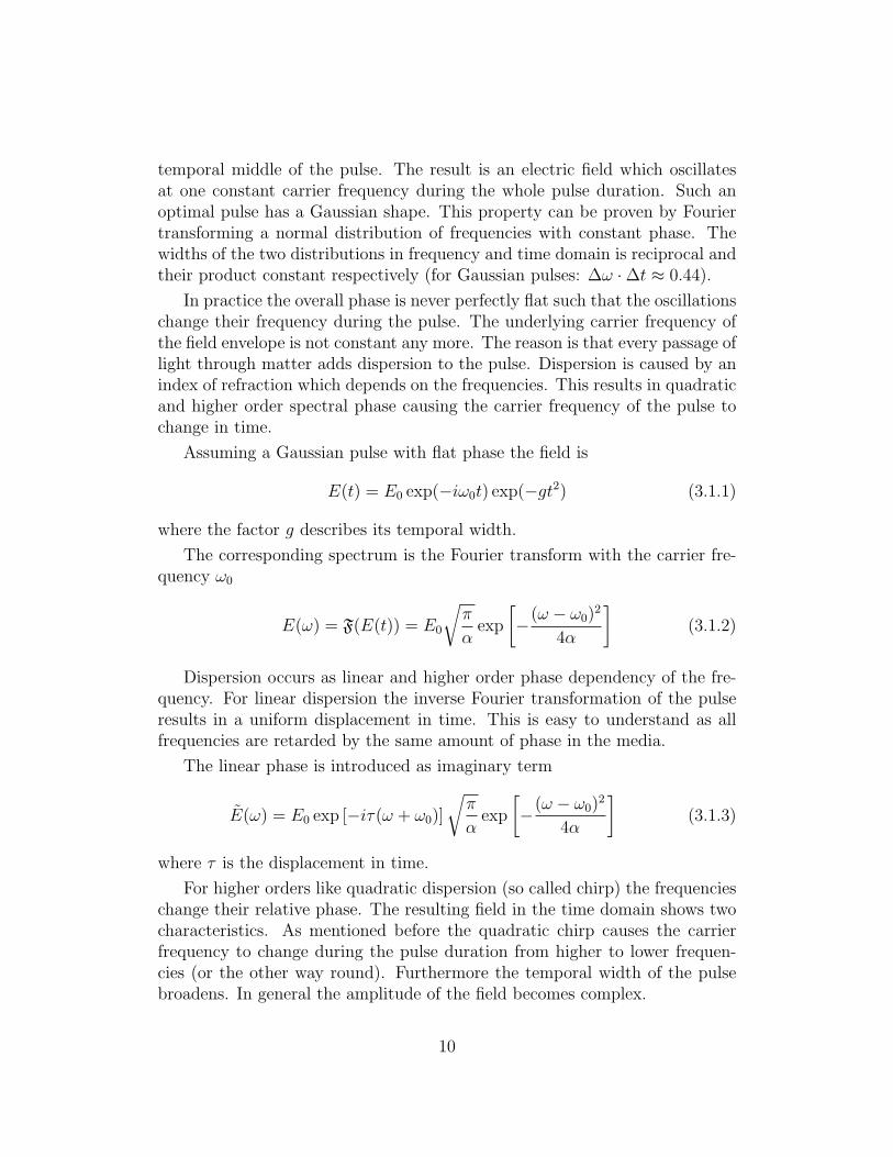
temporal middle of the pulse. The result is an electric field which oscillatesat one constant carrier frequency during the whole pulse duration. Such anoptimal pulse has a Gaussian shape. This property can be proven by Fouriertransforming a normal distribution of frequencies with constant phase. Thewidths of the two distributions in frequency and time domain is reciprocal andtheir product constant respectively (for Gaussian pulses: ∆ω ·∆t ≈ 0.44).

In practice the overall phase is never perfectly flat such that the oscillationschange their frequency during the pulse. The underlying carrier frequency ofthe field envelope is not constant any more. The reason is that every passage oflight through matter adds dispersion to the pulse. Dispersion is caused by anindex of refraction which depends on the frequencies. This results in quadraticand higher order spectral phase causing the carrier frequency of the pulse tochange in time.

Assuming a Gaussian pulse with flat phase the field is

E(t) = E0 exp(−iω0t) exp(−gt2) (3.1.1)

where the factor g describes its temporal width.

The corresponding spectrum is the Fourier transform with the carrier fre-quency ω0

E(ω) = F(E(t)) = E0

√π

αexp

[−(ω − ω0)2

4α

](3.1.2)

Dispersion occurs as linear and higher order phase dependency of the fre-quency. For linear dispersion the inverse Fourier transformation of the pulseresults in a uniform displacement in time. This is easy to understand as allfrequencies are retarded by the same amount of phase in the media.

The linear phase is introduced as imaginary term

E(ω) = E0 exp [−iτ(ω + ω0)]

√π

αexp

[−(ω − ω0)2

4α

](3.1.3)

where τ is the displacement in time.

For higher orders like quadratic dispersion (so called chirp) the frequencieschange their relative phase. The resulting field in the time domain shows twocharacteristics. As mentioned before the quadratic chirp causes the carrierfrequency to change during the pulse duration from higher to lower frequen-cies (or the other way round). Furthermore the temporal width of the pulsebroadens. In general the amplitude of the field becomes complex.

10

(a) (b)

Figure 3.1: Influences of Linear Phase on a Gaussian Pulse. Theoriginal Gaussian pulse (a) is centered at t = t0 whereas the pulse withlinear phase (b) is shifted in time and is centered at t = t0 + τ .

The quadratic phase is introduced similarly

E(ω) = E0 exp[−iβ(ω + ω0)2

]√π

αexp

[−(ω + ω0)2

4α

](3.1.4)

where β is called the spectral chirp rate.

The inverse Fourier transform gives the resulting field

E(t) = E ′0 exp[−i(ω0t+ bt2)

]exp(−at2) (3.1.5a)

E ′0 = E0

√1

1 + i4αβ(3.1.5b)

a =α

1 + 16α2β2(3.1.5c)

b = − 4α2β

1 + 16α2β2(3.1.5d)

The parameter α describes the width of the spectrum (comp. 3.1.4) andthe parameter β is a measure of quadratic change in spatial phase leading toa non constant carrier frequency. Depending on the sign of the chirp rate βthe frequency sweep starts at higher or lower frequencies. The pulse durationas a function of β is

∆t′ =√

1 + 16α2β2 ∆t (3.1.6)

11

(a) (b)

Figure 3.2: Influences of Quadratic Phase on a Gaussian Pulse.The original Gaussian pulse (a) is has the shortest time duration. Aquadratic chirp broadens the pulse (b) in the time domain and causesthe carrier frequency to change during the pulse.

3.2 Pulse Characterization Background

The characterization of an ultra short laser pulse is a challenge. As mentionedearlier, conventional techniques are not able to resolve temporal structures inthe fs -regime. The only measure which is available on this timescale is thepulse itself, hence all characterization methods are based on nonlinear optics.

Autocorrelation is the process of ”comparing” a signal with some processedcopy of itself. In most cases the processing is a simple shift in time so that theautocorrelation function A(τ) could be defined as

A(τ) =

∫f(t) · f(t+ τ)dt (3.2.1)

The Wiener-Khinchin theorem relates the autocorrelation to the power spec-tral density ρ(ω) via Fourier transformation:

A(τ) = F(ρ(ω)) (3.2.2)

In an experimental apparatus this equation could be satisfied by splitting abeam in a beam splitter, shifting one beam in time by a variable path lengthand creating a second harmonic signal in a nonlinear optic (compare figure3.3).

12

Spectrometer

SHG crystal

translation stage

Figure 3.3: Schematic Drawing of FROG Setup. The light is splitby a beam splitter and travels different path lengths due to the transla-tion stage. In the crystal the recombined beams produces a SHG signalmeasured by a spectrometer.

Nonlinear responses like second harmonic generation (SHG) are propor-tional to the intensity of the mixed signal which is the sum of the two mergedbeams I ∝ |Ea + Eb|2 = |Ea|2 + |Eb|2 + 2 |Ea · Eb|. When the coopera-tive signal (|Ea · Eb|) can be separated its intensity will be proportional to|E(t) · E(t− τ)| which is the needed quantity.

The signal is measured with a spectrometer. Scanning the parametersdelay time τ and frequency ω results in a two dimensional (τ, ω) trace whichcontains all information about intensity and phase of the pulse. The resultingdata reads:

S(ω, τ) ∝∣∣∣∣∫ E(t)E(t− τ)eiωtdt

∣∣∣∣2 (3.2.3)

Several different mathematical algorithms can retrieve the pulse by iter-ation of Fourier transformations between time and frequency domains. Themathematical discussion is very complex and can be found in [47].

13

Many different technical realizations have been build. The first and maybebest known is the FROG1 [47]. Further modified approaches follow the ”nam-ing convention” and are called GRENOUILLE2 [2], SPIDER3 [38] and MIIPS4

[24].The configuration and calibration of the GRENOUILLE is described in

chapter 3.

3.3 Design of the GRENOUILLE

The GRENOUILLE [2] is one possible experimental apparatus to measure thefield and phase of an ultrafast laser pulse. Its name is the French name for frogand stands for ”Grating-Eliminated No-nonsense Observation of UltrafastIncident Laser Light E-fields”.

The goal of this particular realization is to record the autocorrelation (com-pare equation 3.2.1) trace with a CCD5 camera in one shot. Its setup can bedivided into two functional groups, one which resolves the time and one whichresolves the frequency. In the FROG approach, time is resolved by a vari-able path length and the frequency is measured with a spectrometer. TheGRENOUILLE performs both tasks in a nonlinear crystal, the time resolu-tion in the horizontal plane (top view) and the spectral analysis in the verticalplane (side view). A key feature is the thick second harmonic generation (SHG)crystal (3).

Figure 3.4 shows a sketch of both views allowing to demonstrate the pur-pose of every single element. Before the beam enters the apparatus the beamis enlarged to a diameter of about one centimeter.

Following the top view path illustrates the time resolution mechanism. Thebroadened beam passes through the cylindrical lens (1) without change. Thislens becomes important in the frequency resolution path. Subsequent the beamenters the Fresnel biprism (2) with an apex angle of 170. It is creating twocrossing beams coming to complete overlap in the thick SHG crystal (3) in thehorizontal plane. The beams could be regarded as plane waves at this pointso that they meet each other at a fixed angle in the crystal. This leads to asituation in which the path length difference of two crossing parts of the beams

1Frequency Resolved Optical Gating2GRating-Eliminated No-nonsense Observation of Ultrafast Incident Laser Light E-fields3Spectral Phase Interferometry for Direct Electric field Reconstruction4Multiphoton Intrapulse Interference Phase Scan5charge-coupled device, electronic light sensor

14

x

f/2(1) (2) (3) (4) (6)(5)

(5)

both 50mm10mm

100mm

w

f(1) (2) (3) (4) (6)

150mm 100mm

(a): top

(b): side

Figure 3.4: Side and Top View of a GRENOUILLE Setup. Thefigure part (a) with the top view shows the time resolution beam path, thefigure part (b) the frequency resolution beam path. The elements are thefollowing: (1) cylindrical lens, (2) Fresnel biprism, (3) thick SHG crystal,(4) imaging lens with focii f/2 for top view and f for side view, (5) slitand (6) CCD camera

only depends on their horizontal position in the crystal. Along the middle ofthe crystal the difference is zero and scales linear towards the edges.

Therefore the width of the beam in the crystal (about 4 mm) in conjunctionwith the biprism apex angle determines the possible path differences betweenthe two beams. Knowing the speed of light in the crystal (index of refractiongiven in figure 3.5) one can derive the maximum time delay between the beams.

The thick crystal is made from a material with a high nonlinear response.Potassium Dihydrogen Phosphate (KDP) with a length of 10 mm is used inour setup. Three different beams of second harmonic light will come out ofthe crystal. Two are parallel to the incoming beams. They are created byfrequency doubling in the single beams. They do not comprise any informationabout the autocorrelation, hence these beams are filtered by the slit (5).

15

The third signal is the cooperative one being created by one photon ofeach beam. Due to conservation of momentum this beam comes out parallelto the beam before the biprism. It is the autocorrelation between the pulses.Depending on where in the crystal the process takes place, the incoming pulsesare shifted in time. Hence the outcoming light provides the time resolutionmapped to space in the horizontal plane. The signal can be imaged with anadditional lens (4) (focal length of 50 mm in this plane) to a CCD chip (6).Images can be taken with a resolution of 1280× 1024 pixel.

The spectral resolution (side view) works differently. To create SH lightin a non-linear crystal, both the incoming and the SH beam must be phasematched as the group velocities of the two beams in the crystal usually differdue to dispersion. This is especially the case if the crystal is thick.

Birefringence nevertheless allows to phase match the beams by choosingdifferent projections of ordinary and extraordinary polarization for the beams.The condition on the refractive indices n1 and n2 for matching the groupvelocities of the frequencies ω and 2ω is

c/n1(ω) = c/n2(2ω) (3.3.1)

This can be satisfied by tilting the crystal by some angle, namely the phase-matching angle α. The beams then see a combination of no and neo. Theformula to calculate the right angle for a frequency ω is

sin (α(ω, 2ω))2 =no(ω)−2 − no(2ω)−2

neo(2ω)−2 − no(2ω)−2(3.3.2)

for a negative birefringent crystal. The tolerance within the angle for a certainwavelength mainly depends on the thickness of the crystal. Longer paths inthe crystal imply more destructive interference for imperfectly matched SHlight and therefore a smaller tolerance.

The issue of phase matching is the key to the spectral resolution. Everysingle wavelength has a certain phase matching angle. A single wavelengthgoing into the crystal at its phase matching angle produces constructivelyinterfering SH photons whereas every different wavelengths has destructiveinterference at this angle.

Therefore a thick crystal produces spectrally resolved SH light by mappingwavelength to different angles. The setup is designed such that the beamscome in focused by an angle large enough to cover all phase matching angles.For wavelengths between 720 nm and 850 nm the beam focusing angle has tobe greater than 5.6 and the crystal axis tilted by 46.1. A cylindrical lens (1)

16

in front of the biprism which only influences the vertical plane will guaranteethis focus. Afterwards the SH signal is imaged onto the CCD chip with the lens(4). The imaging lens has a different focal length of 100 mm for the verticalplane.

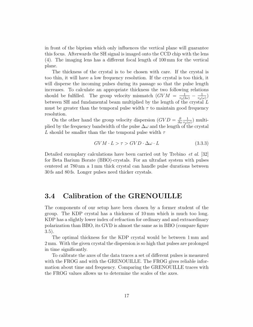
The thickness of the crystal is to be chosen with care. If the crystal istoo thin, it will have a low frequency resolution. If the crystal is too thick, itwill disperse the incoming pulses during its passage so that the pulse lengthincreases. To calculate an appropriate thickness the two following relationsshould be fulfilled. The group velocity mismatch (GVM = 1

vg(2ω)− 1

vg(ω))

between SH and fundamental beam multiplied by the length of the crystal Lmust be greater than the temporal pulse width τ to maintain good frequencyresolution.

On the other hand the group velocity dispersion (GVD = ∂∂ω

1vg(ω)

) multi-

plied by the frequency bandwidth of the pulse ∆ω and the length of the crystalL should be smaller than the the temporal pulse width τ

GVM · L > τ > GVD ·∆ω · L (3.3.3)

Detailed exemplary calculations have been carried out by Trebino et al. [32]for Beta Barium Borate (BBO)-crystals. For an ultrafast system with pulsescentered at 780 nm a 1 mm thick crystal can handle pulse durations between30 fs and 80 fs. Longer pulses need thicker crystals.

3.4 Calibration of the GRENOUILLE

The components of our setup have been chosen by a former student of thegroup. The KDP crystal has a thickness of 10 mm which is much too long.KDP has a slightly lower index of refraction for ordinary and and extraordinarypolarization than BBO, its GVD is almost the same as in BBO (compare figure3.5).

The optimal thickness for the KDP crystal would be between 1 mm and2 mm. With the given crystal the dispersion is so high that pulses are prolongedin time significantly.

To calibrate the axes of the data traces a set of different pulses is measuredwith the FROG and with the GRENOUILLE. The FROG gives reliable infor-mation about time and frequency. Comparing the GRENOUILLE traces withthe FROG values allows us to determine the scales of the axes.

17

400 500 600 700 800wavelength [nm]

1.561.581.6

1.621.641.661.68

n

(a)

400 500 600 700 800wavelength / nm

1.471.481.491.5

1.511.52

n

(b)

Figure 3.5: Indices of Refraction for BBO and KDP. The graphsshow the dispersion curves of BBO (a) and KDP (b) for ordinary (highestline), extraordinary (lowest line) and 45 (middle line) polarization. Thevalues have been calculated with the Sellmeier equations.

A GRENOUILLE trace of a transform limited pulse looks like a two di-mensional Gaussian distribution. Its relation between horizontal and verticalexpansion depends on the setup. In our setup the traces have a cigar shape.Typical autocorrelation shapes can be found in [47]. For pulses with a spatialchirp the trace is tilted [1]. The angle indicates for a specific apparatus theamount of spatial chirp.

Figure 3.6 shows the GRENOUILLE trace of a 36 fs pulse taken by a CCDcamera. Pixels in the horizontal dimension represent the time scale and pixelsthe vertical dimension the frequency scale. The shape is the predicted cigarshape with some small distortions. Dust on the CCD chip produces dark spots.Some other spots show an Airy pattern. They might come from diffractionby small distortions or dust on the optics. The inserted line in the lower partillustrates the shape of the projection onto the time axis.

For the calibration it is important to recall the reasons for different pulseduration with equal frequency bandwidth. Most pulses in experiments donot have the minimal temporal width they could have comparing with thetransform limited pulse duration. The reason is that every pulse picks up apositive second order phase (compare chapter 3.1 about chirped pulses) bytraveling through optics. Pulse durations prolong with the absolute amountof the phase (hence are independent from its sign).

For the calibration of the GRENOUILLE a set of pulses with different pulseduration is created by actively introducing such a second order phase. TheFROG, which has very small internal dispersion (there are no lenses and just a

18

pixel horizontal

pixe

l ver

tical

200 400 600 800 1000 1200

100

200

300

400

500

600

700

800

900

1000

10

20

30

40

50

60

Figure 3.6: GRENOUILLE Trace of Short Pulse. The trace of a 36 fspulse taken with a CCD camera looks like a cigar and is almost symmetric.The horizontal dimension represents the time scale, the vertical dimensionthe frequency scale. Dust on the optics produces the dark spots. Theinserted line illustrates the shape of the projection onto the time axis.

very thin crystal) does not change the phase during measurement. In contrastto this, the GRENOUILLE introduces a fixed amount of positive chirp. Fora transform limited pulse this leads to a longer duration but for pulses withnegative phase distortion the GRENOUILLE compensates to some amountand can even shorten the pulse.

As result the relation between the pulse duration in the FROG and thepulse duration in the GRENOUILLE is not linear. There even occurs anambiguity in the calibration. With a thinner crystal this problem would bemuch smaller but the current setup has to take it into account.

There is no way to use the CCD camera data for reconstruction. Thealgorithm can not compensate for the ambiguity. Nevertheless the width ofthe autocorrelation is a reliable measure of the pulse duration for simple pulses.

It is important to find a robust way to measure the width of the pixel

19

distribution. We chose to take the average FWHM of all horizontal lines.This value represents the mean of all frequencies. Thus the algorithm is notinfluenced much by distortions as seen in the image above. The inserted linein figure 3.6 allows us to determine the FWHM.

(a)

(b)

FRO

G p

ulse

dur

atio

n [fs

]

180

160

140

120

100

80

60

40

20

0

pixel0 20 40 60 80 100 120 140 160

Figure 3.7: GRENOUILLE Pulse Duration Calibration. The cal-ibration trace shows the FROG pulse durations measured in dependenceof the pixel width of the distribution from the CCD camera. Due to thedispersion in the thick KDP crystal the curve is not linear and shows anambiguity. Phases for data points (a) and (b) are shown in figure 3.9.

Figure 3.7 shows the calibration data. The run of the curve shows clearlythat minimal pulse duration in the FROG and narrowest pixel distribution donot coincide.

The shortest pulse (30 fs) has a width of 54 px whereas the smallest pixelwidth (28 px) has a pulse duration of 58 fs. A pulse of 58 fs has exactly theamount of negative chirp which the crystal and the lenses introduces positively.Hence the pixel width becomes minimal. Every measured value broader than28 pixels corresponds to two possible pulses: one is longer than 58 fs, hasnegative chirp and is compressed (upper branch) and the other one is shorter

20

than 58 fs, has positive chirp and is stretched (lower branch).Figure 3.8 shows a reconstructed pulse with its intensity and phase. One

can see that the pulse has a flat temporal phase. This pulse corresponds tothe FROG minimum with 28 fs.

700 750 800 850 9000

0.1

0.2

0.3

0.4

0.5

0.6

0.7

0.8

0.9

1

wavelength [nm]

inte

nsity

[nor

m]

0

0.5

1

1.5

2

2.5

3

phas

e [R

ad]

Figure 3.8: Pulse with Flat Phase. This pulse is the shortest FROGmeasure and has a flat phase throughout its intense parts. The solid lineshows the intensity in time, the dashed line indicates the phase. It is flat inthe main region of the pulse. The wings of the pulse have a small influenceon the pulse.

The second pulse shown in figure 3.9 has a negative chirp though it is shownpositively. SHG reconstruction does not allow us to determine the sign of thephase so that the algorithm picks it randomly. This pulse corresponds to theGRENOUILLE minimum. It has exactly the right amount of negative chirpto be compensated in the crystal. The result is a narrowest in pixels.

To use the GRENOUILLE as a fast measure for the pulse duration, thelower branch of the calibration data is fitted. Assuming that the pulse isalready close to its optimal duration (which means it is on this branch) thefitted function allows us to determine the pulse duration in real time. Anotherstudent (Brendan Keller) of the group has written the LabVIEW code for the

21

CCD camera.

700 750 800 850 9000

0.1

0.2

0.3

0.4

0.5

0.6

0.7

0.8

0.9

1

wavelength [nm]

inte

nsity

[nor

m]

0

1

2

3

4

5

6

7

8

phas

e [R

ad]

Figure 3.9: Pulse with Quadratic Phase. This pulse has the narrowestpixel width in the GRENOUILLE and a negative phase which is compen-sated by the crystal. The solid line shows the intensity and the dashedline the phase in time. (The phase is shown positively as the retrievalalgorithm cannot determine its sign.)

The fitted function is

τ(∆x) = (593.68− 46.542∆x+ 1.559(∆x)2 − 0.02703(∆x)3 + 0.00026(∆x)4) fs(3.4.1)

where τ is the pulse duration in fs and ∆x the pixel width.The error bars in figure 3.7 indicate the spread of three different traces

taken for every data point. For short and simple pulses the results of theGRENOUILLE measurement are well reproducible. The mean error in thepulse duration is ± 1.5 fs. This error adds to the unknown error of the FROG.The guess for the overall error is < ± 3 fs. Determining the pulse durationis rather insensitive to the alignment. Misaligned beams are displaced on the

22

CCD camera but their width stays almost constant.w

avel

engt

h [n

m]

∆ pixel

804

800

796

792

788

784

780

776

772

768

100 200 300 400 500 600 700 800 900

Figure 3.10: GRENOUILLE Wavelength Calibration. The curveshows the measured frequency dependence from the position on the CCDcamera.

Shaped pulses with complicated phases cannot been measured with theGRENOUILLE. For this reason it is mainly used to check the amplifier output.

A wavelength calibration is carried out with the pulse shaper. Narrowbandwidth pulses are measured in the GRENOUILLE. Reference spectra havebeen measured with a spectrometer. The relation between the position on theCCD camera and the wavelength is to good approximation linear. Figure 3.10shows the data. It was fitted to

λ(x) = (808.9− 0.024x) nm (3.4.2)

with the wavelength λ in nm and the position x on the CCD camera in pixel.This calibration is less important as it does not give more information than ausual spectrometer. Furthermore it is highly dependent on correct alignment.

With the time calibration the GRENOUILLE is used on an every day basis

23

for monitoring the pulse duration.

24

Chapter 4

Theoretical Background

The understanding of ultrafast pulses and their interaction with matter re-quires a detailed description of the electric field and its interplay with atomicstates. Many assumptions known from ”traditional” optics do not hold true inthe fs-regime. Therefore the following chapter will discuss the most importantfeatures of ultrafast pulses interacting with atoms. Furthermore the chemicalelement Rubidium is presented with its important properties.

4.1 Two-Level-Atoms

Real atoms usually have very complex internal structures with numerous en-ergy levels. Nevertheless most experiments are designed to limit the amountof states which take part in the processes. In a lot of cases the number ofrelevant levels can be reduced to two or else two levels mainly determine thedynamics of the atomic system. So the behavior of two-level-atoms has beenstudied comprehensively.

The following chapter explains one approach to two-level-atoms. It is im-portant to notice that the process of spontaneous emission is not taken intoaccount in this picture. Introducing the concept of Rabi cycling leads to a de-scription of these systems in terms of intensity and detuning. The treatmentof two-level-atoms follows Tannor [43]. A similar derivation can be found inBoyd [8].

The Hamiltonian for these two-level-atoms has the two eigenstates Ψa andΨb with the energies Ea = ~ωa and Eb = ~ωb respectively. The transitionfrequency is ω0 = ωb − ωa.

25

The general wave function for the two-level-atoms thus reads:

Ψ(t) = a(t)e−iωatΨa + b(t)e−iωbtΨb (4.1.1)

The square of the coefficients |a(t)|2 and |b(t)|2 represent the probabilitiesof finding an electron in state Ψa or Ψb respectively. A light field interactswith the states via the dipole moment µ and produces the coupling termV = −µabε(t). Writing the time-dependent Schrodinger equation in matrixform leads to

i~d

dt

(a(t)e−iωat

b(t)e−iωbt

)=

(Ea −µabε(t)

−µbaε(t) Eb

)(a(t)e−iωat

b(t)e−iωbt

)(4.1.2)

The electric field is considered to be CW field with a single frequency so thatit can be written as ε(t) = 1/2 ε·(eiωt + e−iωt) and the two dipole moments areequal µab = µba = µ. This results in a system of coupled differential equations

a(t) = iµε

2~(e+i(ω−ω0)t + e−i(ω+ω0)t

)b(t) (4.1.3a)

b(t) = iµε

2~(e−i(ω−ω0)t + e+i(ω+ω0)t

)a(t) (4.1.3b)

The detuning is defined as ∆ = ω − ω0. For the next step the rotatingwave approximation is applied. This means that all fast oscillating terms likee+i(ω+ω0)t are considered to average to zero. In this case the RWA is a verygood approximation as the detuning is orders of magnitudes smaller than thetransition frequency. Hence we ignore the term.

a(t) = iµε

2~e+i∆tb(t) (4.1.4a)

b(t) = iµε

2~e−i∆ta(t) (4.1.4b)

A good trial for the solution for the state Ψa is made by

a(t) = Cae−iβt (4.1.5)

which results in the equation for state Ψb

b(t) = −Ca2~βµε

e−i(∆+β)t (4.1.6)

26

Using the last two equations with 4.1.4b leads to the condition

β(∆ + β) =(µε

2~

)2

(4.1.7)

The Rabi frequency is introduced as Ω = µε/~ so that the solution for βis given by

β± = 1/2(

∆±√

∆2 + Ω2)

= 1/2(

∆± Ω)

(4.1.8)

The generalized Rabi frequency Ω =√

∆2 + Ω2 plays the central role inthis description of the two-level-atoms.

Substituting back β into equations 4.1.4 leads to the general solutions

a(t) = − 1

Ωe+ i

2∆t(A(∆− Ω)e+ i

2Ωt +B(∆ + Ω)e−

i2

Ωt)

(4.1.9a)

b(t) = e−i2

∆t(Ae+ i

2Ωt +Be−

i2

Ωt)

(4.1.9b)

Choosing the initial conditions to be |a(t0)|2 = 1 and |b(t0)|2 = 0 definesthe constants A = −B = µε/(2~Ω). To obtain the populations the solutionsare squared and read

|a(t)|2 =

(∆

Ω

)2

+

(Ω

Ω

)2

cos2(Ωt/2) (4.1.10)

|b(t)|2 =

(Ω

Ω

)2

sin2(Ωt/2) (4.1.11)

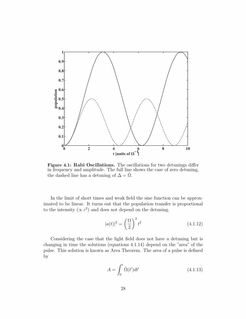
The population of excited state Ψb is plotted in figure 4.1. It rises from zeroto a maximal amount and oscillates between these two values. The maximalpopulation transfer is given by the ratio Ω/Ω, its frequency is given by Ω/(4π).The population transfer is unity for a light field without detuning and smallerfor all fields with non-zero detuning.

Figure 4.1 illustrates this behavior for two different generalized Rabi fre-quencies. As the frequencies of the sinusoidal parts depend on Ω the two caseshave different transfer rates.

It is important to keep in mind that this picture does not take into accountthe spontaneous emission which would decrease the population of state Ψb

and hence lead to some kind of steady state behavior (treated for instance inMetcalf [28]).

27

0 2 4 6 8 100

0.1

0.2

0.3

0.4

0.5

0.6

0.7

0.8

0.9

1po

pula

tion

t [units of Ω−1]

Figure 4.1: Rabi Oscillations. The oscillations for two detunings differin frequency and amplitude. The full line shows the case of zero detuning,the dashed line has a detuning of ∆ = Ω.

In the limit of short times and weak field the sine function can be approx-imated to be linear. It turns out that the population transfer is proportionalto the intensity (∝ ε2) and does not depend on the detuning.

|a(t)|2 =

(Ω

2

)2

t2 (4.1.12)

Considering the case that the light field does not have a detuning but ischanging in time the solutions (equations 4.1.14) depend on the ”area” of thepulse. This solution is known as Area Theorem. The area of a pulse is definedby

A =

∫ t

0

Ω(t′)dt′ (4.1.13)

28

such that the populations read

a(t) = cos

(1

2

∫ t

0

Ω(t′)dt′)

(4.1.14a)

b(t) = i sin

(1

2

∫ t

0

Ω(t′)dt′)

(4.1.14b)

The importance of the area theorem is that the Rabi cycling in the case ofvarying fields does not depend on the particular field shape but just on itsintegral. It is easy to see from equations 4.1.14 that total inversion happensin the case when the ares is equal to π - a so called π-pulse.

4.2 Dressed States

In the dressed state picture, the influence of the presence of a light field istreated. As long as two-level-atoms are situated in the dark the previouslydescribed states Ψa and Ψb (see chapter 4.1) are the bare eigenstates of thesystem. The Hamiltonian is a diagonal matrix and its elements are the eigenen-ergies. This does not hold true any more when the coupling terms appear inthe off-diagonal matrix elements of the Hamiltonian. New eigenstates whichare superpositions of Ψa and Ψb occur with new eigenenergies.

This chapter introduces the most important changes when taking into ac-count a combined system of atom and field. The calculations follow Tannor[43].

To address this problem we first calculate the expectation value of thedipole moment with the solutions of the two-level-atoms. This treatment showsthat new transition frequencies occur at ω ± Ω.

For determining the expectation value of the dipole moment we evaluate

〈µ(t)〉 = 〈Ψ(t) |µ|Ψ(t)〉 (4.2.1)

The dipole moment depends linearly on the integration coordinate r sothat 〈Ψa |µ|Ψa〉 = 〈Ψb |µ|Ψb〉 = 0. Going back to the definition of the wavefunction Ψ in equation 4.1.1 the expectation value reads

〈µ(t)〉 = a∗(t)b(t)µe−iωbat + c.c. (4.2.2)

with the coefficients a(t) and b(t).

29

ω ω

Δ

Δ

ωb

ωa

ω

ω

Ω

Ωωa- 1/2(Δ - Ω)

ωb+ 1/2(Δ + Ω)

ωb+ 1/2(Δ - Ω)

ωa- 1/2(Δ + Ω)

ω + Ω ω - Ω

~

~

~

~

~~

~

~

(a) Dressed State Weak Field (b) Dressed State Strong Field

Figure 4.2: Dressed State Spectrum. (a) In the weak field regime twonew levels occur with an offset of ∆ such that the light field is resonantwith them. (b) In the strong field regime there are three different transitionfrequencies ω, ω± Ω between the two dressed states. Both figures assumethat the detuning is positive.

Plugging in solutions 4.1.9 from the two-level-derivation for a(t) and b(t),with the given integration parameters A and B, leads to the expression

〈µ(t)〉 = − Ω

4Ω2

[2∆e−iωbat −

(∆− Ω

)e−i(ωba+Ω)t

−(

∆ + Ω)e−i(ωba−Ω)t

]µab + c.c. (4.2.3)

This solution shows that the dipole moment oscillates at the fundamentaland two new frequencies ω ± Ω. The reason for the behavior is that alreadythe coefficients a(t) and b(t) oscillate at frequencies different from the lightfield. This is called Mollow triplet [30]. Figure 4.2(b) draws a sketch of thetransitions.

In the case of zero detuning the dipole moment oscillates just at the twonew different frequencies

〈µ(t)〉 = − Ω

4Ω

[e−i(ωba+Ω)t − e−i(ωba−Ω)t

]µab + c.c. (4.2.4)

There is no oscillation at the original frequency. The absorption line is splitinto two lines with a spacing proportional to the Rabi frequency.

As mentioned above, the dressed states can be regarded as superposition

30

of the atom’s bare eigenstates. Going back to the solutions for a(t) and b(t)in equations 4.1.9 one can choose the integration parameters A and B to fitdifferent initial conditions. One possible case is the combination A = 0 andB = 1 which is identified as Ψ+. Likewise the combination A = 1 and B = 0is also possible and is labeled Ψ−.

Equation 4.1.9 read now

a+(t) = −∆ + Ω

Ωe−

i2

(Ω−∆)t (4.2.5a)

b+(t) = e−i2

(∆+Ω)t (4.2.5b)

a−(t) = −∆− Ω

Ωe

i2

(Ω+∆)t (4.2.5c)

b−(t) = e−i2

(∆−Ω)t (4.2.5d)

We plug these coefficients into the definition of the wave function Ψ 4.1.1and normalize the solutions. The resultant wave function composes of Ψa andΨb.

Ψ± = ∓

√Ω±∆

2Ωexp

[+i

(∆∓ Ω

2− ωa

)t

]Ψa

±

√Ω∓∆

2Ωexp

[−i

(∆± Ω

2+ ωb

)t

]Ψb (4.2.6)

These functions are the new eigenstates of the combined system of atom andfield. The can be regarded as the eigenvector of the instantaneous Hamiltonian.Note that they do not give the eigenenergies as the Hamiltonian is explicitlytime-dependent.

Projecting the functions Ψ± onto the bare eigenstates shows that the prob-ability of finding the system in Ψa/b is constant in time and hence that theyare stationary states

|〈Ψa|Ψ±〉|2 =Ω±∆

2Ω(4.2.7a)

|〈Ψb|Ψ±〉|2 =Ω∓∆

2Ω(4.2.7b)

31

For weak fields (Ω << ∆) one can approximate the generalized Rabi fre-quency to

Ω ≈ |∆|

[1 +

(Ω

∆

)2]

(4.2.8)

Assuming positive detuning the dressed states reduce to

Ψ+ = −√

1− Ω2

2∆2e−iωatΨa +

Ω√2∆

e−i(ωb+∆)tΨb (4.2.9a)

Ψ− =Ω√2∆

e−i(ωa−∆)tΨa +

√1− Ω2

2∆2e−iωbtΨb (4.2.9b)

Solution Ψ+ is dominated by the bare eigenstate Ψa and Ψ− by Ψb re-spectively. Both have small corrections of the other bare eigenstate with anew frequency associated which can be regarded as newly introduced level(compare figure 4.2(a)).

For some quantum mechanical problems it can be convenient to work in theinteraction picture. This picture is intermediate between the Heisenberg andSchrodinger picture and evolves from them by an unitary transformation U .In the interaction picture the Hamiltonian is split into two parts H = H0 + Vwhere H0 denotes a well known Hamiltonian which is exactly solvable. Thepart V usually contains new terms which make the Hamiltonian more complex.Any arbitrary choice of the two parts is valid. When chosen properly the timeevolution in the new picture can be much slower than in the other ones.

The new wave function reads

Ψi(t) = ei/~H0tΨs(t) = ei/~H0te−i/~HtΨs(0) (4.2.10)

where Ψs represents the wave function in the Schrodinger picture.The Hamiltonian in the Schrodinger picture is

Hs =

(Ea −µε(t)

2e−iωt

−µε(t)2e−iωt Eb

)(4.2.11)

32

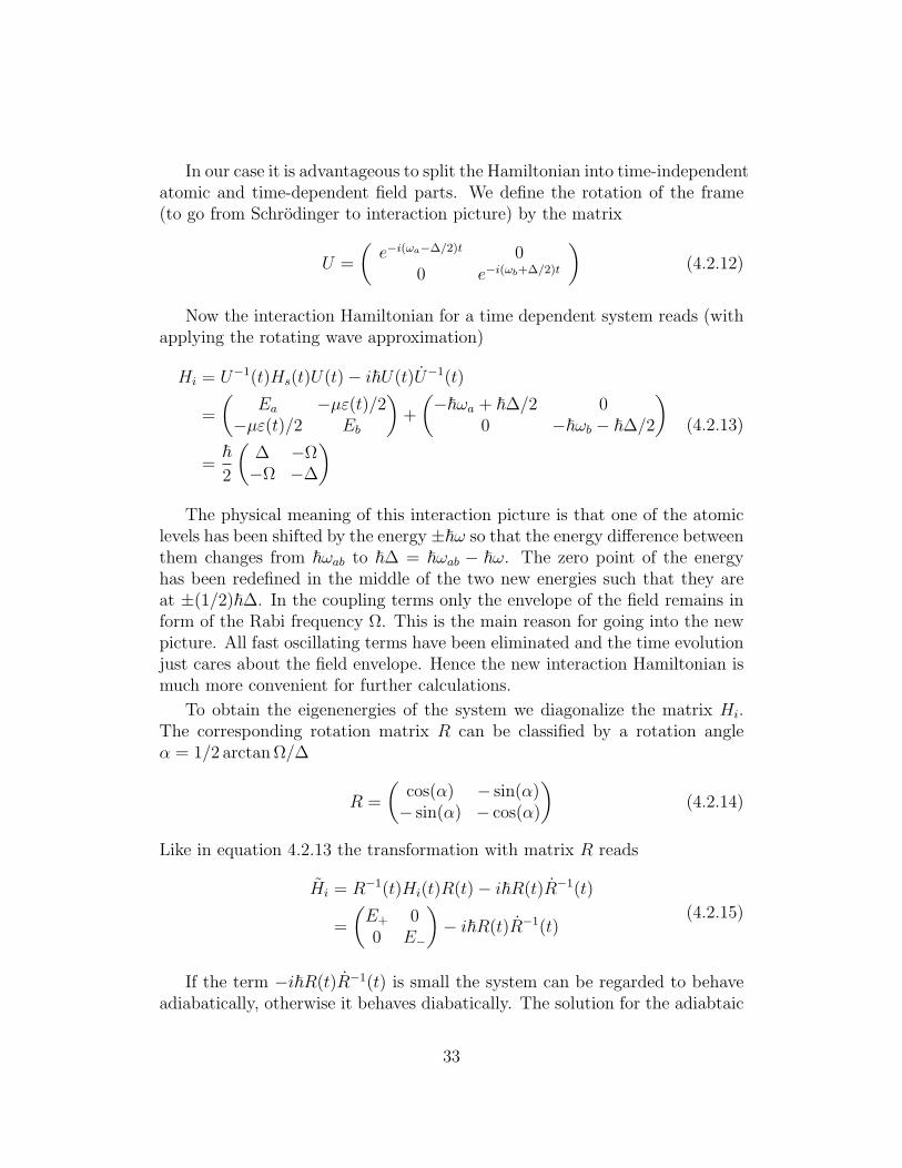
In our case it is advantageous to split the Hamiltonian into time-independentatomic and time-dependent field parts. We define the rotation of the frame(to go from Schrodinger to interaction picture) by the matrix

U =

(e−i(ωa−∆/2)t 0

0 e−i(ωb+∆/2)t

)(4.2.12)

Now the interaction Hamiltonian for a time dependent system reads (withapplying the rotating wave approximation)

Hi = U−1(t)Hs(t)U(t)− i~U(t)U−1(t)

=

(Ea −µε(t)/2

−µε(t)/2 Eb

)+

(−~ωa + ~∆/2 0

0 −~ωb − ~∆/2

)=

~2

(∆ −Ω−Ω −∆

) (4.2.13)

The physical meaning of this interaction picture is that one of the atomiclevels has been shifted by the energy ±~ω so that the energy difference betweenthem changes from ~ωab to ~∆ = ~ωab − ~ω. The zero point of the energyhas been redefined in the middle of the two new energies such that they areat ±(1/2)~∆. In the coupling terms only the envelope of the field remains inform of the Rabi frequency Ω. This is the main reason for going into the newpicture. All fast oscillating terms have been eliminated and the time evolutionjust cares about the field envelope. Hence the new interaction Hamiltonian ismuch more convenient for further calculations.

To obtain the eigenenergies of the system we diagonalize the matrix Hi.The corresponding rotation matrix R can be classified by a rotation angleα = 1/2 arctan Ω/∆

R =

(cos(α) − sin(α)− sin(α) − cos(α)

)(4.2.14)

Like in equation 4.2.13 the transformation with matrix R reads

Hi = R−1(t)Hi(t)R(t)− i~R(t)R−1(t)

=

(E+ 00 E−

)− i~R(t)R−1(t)

(4.2.15)

If the term −i~R(t)R−1(t) is small the system can be regarded to behaveadiabatically, otherwise it behaves diabatically. The solution for the adiabtaic

33

energy

Ea

Eb

E+

E-

Ea

Eb

time

Figure 4.3: Eigenenergies of Dressed States. The adiabatic eigenen-ergies of dressed states for a detuned light pulse start in the bare eigen-states with energies Ea/b, evolves in the dressed states with energies E±and returns to the bare eigenstates.

eigenenergies E± reads

E± = ±~2

√∆2 + Ω2 = ±~

2Ω (4.2.16)

Figure 4.3 shows the time evolution of the the energies E± for a detuned lightpulse. In case the detuning ∆ is much larger than the Rabi frequency Ω theeigenenergies can be developed as

E± ≈ ±~2

(∆ +

Ω2

2∆+ ...

)(4.2.17)

The second term of the development (without the prefactor ~) is the frequencyAC Stark shift

SAC =Ω2

4∆(4.2.18)

34

Chapter 5

Electromagnetically Induced Transparency in

Rubidium

Electromagnetically induced transparency (EIT) is a mechanism to render anoptically dense system transparent. It has been observed in many different ex-periments and can be used for a broad variety of applications. Stephen Harriset al. were the first to both describe theory [20] and carry out experiments[7, 19]. EIT has mainly been observed in atomic systems and but there areexperiments in solids as well by Ham et al. [18].

Most experiments up to now have been carried out in the perturbative fieldstrength regime and many aspects of the phenomena are well understood. Inthis domain the dynamics of the system are described with a perturbationtheory solution of the three-level-atom.

However the exploration of EIT with strong and ultrafast fields has juststarted. Our experiments introduce a time domain perspective to EIT. Thenew aspects in this picture are based on two circumstances: On the one handdephasing mechanisms are much slower than the excitation such that coherencebetween states can be maintained during the whole interaction. On the otherhand field envelopes vary very rapidly in time and for this reason influence thedynamics.

35

5.1 Properties of Rubidium

5S1/2

5P3/25P1/2

5D3/26P3/2

776nm

780nm

762nm

795nm

420nm

5720nm

Figure 5.1: Rubidium EnergyDiagram. The dashed lines showmost important transitions. Alllines connecting to 5P states liewithin the bandwidth of the laser.

Rubidium (Rb) is a silvery-white lookingalkali metal. It is very soft and like mostof the alkali metal highly reactive withoxygen and water. Two natural isotopesoccur with 85 (72.17%) and 87 (27.83%)nucleons.

Rb-87 is slightly radioactive with anuclear life time of 4.88 · 1010 years.The melting point at atmospheric pres-sure is 39.31C, the boiling point is at668C. Its atomic mass is 86.91u = 1.443·10−25 kg. Ionization is observed for ener-gies larger than 4.177 eV = 33690 cm−1.

Rubidium has 37 electrons which allexcept one are located in fully occu-pied orbitals. Almost all physical andchemical processes comprise just this sin-gle valence electron leading to an easyhydrogen like description. The groundstate is 52S1/2 with the configuration4p65s. The following energy diagram5.1 (taken from NIST Atomic SpectraDatabase [34]) shows the atomic levels.

Four transitions lie within the band-width of the laser. Two of them leadfrom the ground state 5S to the interme-diate levels 5P1/2 and 5P3/2. The othertwo transitions lead from the intermedi-ate levels to the upper level 5D3/2. In the following experiments the transitions5S1/2 → 5P3/2 and 5P3/2 → 5D3/2 are used for the EIT, all four transitions areused for the superfluorescence.

All wavelengths and dipole moments are listed in table 5.1. The dipolemoment for the 5P1/2 → 5D3/2 is unknown but Warren et al. [44] indicatethat it is small in comparison to the other three of the discussed transitions.

36

Table 5.1: Transition Data of Rb

transition λ / nm dipole moment/ 10−29 Cm source

5S1/2 → 5P1/2 794.7 1.967 [34]5S1/2 → 5P3/2 780.0 4.97 [10]5P1/2 → 5D3/2 794.7 — [34]5P3/2 → 5D3/2 775.9 1.50 [10]5D3/2 → 6P3/2 5720 — [34]6P3/2 → 5S1/2 420.2 — [34]

The state 6P3/2 becomes important for the measurements in the section 6.2on superfluorescence.

Rubidium has a hyperfine structure as the nuclei have spin 5/2 (Rb-85) and3/2 (Rb-87). The resultant energy shifts are on the order of 100 MHz. Theseshifts correspond to a wavelength difference of 20 pm being orders of magni-tudes smaller than resolvable with the available spectrometers. Therefore allexperimental data will not be able to resolve the structure.

In quantum mechanics the time evolution of a state is always relative toanother state. It is proportional to the energy difference between the twostates. In the case of the Rubidium the time scale for phase evolution betweenhyperfine levels is of the order of 100 ms which is very long in comparison tothe time scales of the experiments. Hence the evolution can be neglected.

The Einstein Aki coefficients for the 5S1/2 → 5P3/2 and 5P3/2 → 5D3/2

transitions are 3.81 · 107 s−1 and 3.61 · 107 s−1 respectively (taken from NISTdatabase [34]). Calculating the lifetimes of the excited states results in about25 ns. This means that they all are at least four orders of magnitude longerthan the time scale of the experiments. For this reason spontaneous emissioncan be neglected during the experiment. Hence the two-level-atom approxi-mation (see chapter 4.1) which neglects spontaneous emission applies well tothe case of rubidium as long as just a single transition is excited.

The vapor pressure PV in Torr for the liquid phase is given by

log10 PV = 15.882− 4529.6

T+ 0.000586T − 2.991 log10 T (5.1.1)

with the temperature T in K. At low pressures it is satisfactory to assume anideal gas which leads to the density-temperature diagram 5.2.

All numbers - if not indicated differently - are taken from Steck [41].

37

50 70 90 110 130 15010

17

1018

1019

1020

temperature [C]

dens

ity

[m−3

]

Figure 5.2: Rubidium Density Diagram. The curve shows the depen-dence of the rubidium density on temperature.

5.2 Electromagnetically Induced Transparency

The technique of EIT for eliminating resonant transitions has been used inmany experiments. Maybe best known is the application of ”slow light” [21]where EIT is used to generate a system with a very small group velocity.Nonlinear processes can profit strongly from EIT as demonstrated with secondharmonic generation in hydrogen [17]. Furthermore EIT relates to topics likelasing without inversion [37].

EIT in atomic experiments can only be observed in three- (or multi) levelsystems. These either ladder- or lambda-type energy levels have three stateswhich we denote |a〉, |b〉, |c〉 (compare figure 5.3). In the case of a laddersystem one also finds ”ground state”, ”intermediate state” and ”excited state”in some literature. The nomenclature is chosen such that the state |c〉 alwaysconnects to both |a〉 and |b〉. The coupling transition with frequency ωc linksthe states |b〉 and |c〉 and the probe transition with frequency ωp states |a〉 and

38

|c〉 respectively.

|a>

|b>

|c>ωcωp

ωc

ωp

(a)

(b)

|a>

|c>

|b>

Figure 5.3: EIT Level Systems. (a)In a lambda system the levels are la-beled |a〉, |b〉 and |c〉 with the couplingωc and probe ωp transitions frequencies.(b) For ladder systems the |c〉 statescorresponds to the intermediate state.

There is no allowed dipole transi-tion between |a〉 and |b〉.

Understanding EIT requires aquantum mechanical point of view.The key to the description is inter-ference between wave functions ex-cited to |c〉 from two different states,namely |a〉 and |b〉. If both couplingand probe fields are close to reso-nance on their transitions they areintroducing quantum coherence be-tween the states |a〉 and |b〉. Inter-ference reduces the effective transferinto state |c〉 dramatically. This phe-nomena is called coherent populationtrapping (CPT) [3].

The levels in figure 5.3 are dressedby the light field. When the lightfield appears as off-diagonal elementsin the Hamiltonian, the bare statesof the atoms evolve to dressed states|p,m〉 which are coherent superposi-tion of the bare states |a〉 and |b〉.Considering the light fields to beprobe (with Rabi frequency Ωp) andcoupling (with Rabi frequency Ωc)fields the dressed states are

|p,m〉 ∝ Ωp |b〉 ± Ωc |a〉 (5.2.1)

where Ωc and Ωp denote the couplingand probe Rabi frequencies.

We calculate the expectationvalue of the dipole operator µ for thetwo levels |c〉 and |m〉

|〈c| µ |m〉|2 ∝ |〈c| µ (Ωp |b〉 − Ωc |a〉)|2 ∝ |ΩcΩp − ΩpΩc|2 = 0 (5.2.2)

39

−2 −1.5 −1 −0.5 0 0.5 1 1.5 20

0.1

0.2

0.3

0.4

0.5

0.6

0.7

0.8

0.9

1

∆ [units of γ]

norm

. abs

orbt

ion

(a) (b)

Figure 5.4: Imaginary part of the susceptibility. The absorption linefor zero coupling (a) splits into two lines (b) for a coupling Rabi frequencyof Ωc = 2γ.

The result from the vanishing expectation value of the dipole moment isthat atoms put into state |m〉 cannot be excited any more to state |c〉. Conse-quently they do not contribute any more to absorption processes. Furthermorethere is no dipole moment that connects the two superpositions |p〉 and |m〉.Hence population - once transfered to |m〉 - is trapped in this state. As therate of population transfer into this state is nonzero for all times populationaccumulates in the trapped state and does not take part any more in thedynamics.

This behavior leads to EIT in the case that a coupling field εc introducesthe coherences on the |b〉 → |c〉 transition. A probe field εp on the |a〉 → |c〉transition has no population to interact with. Hence the usually optical densetransition is transparent.

The time scales on which the EIT forms depends on whether the initialstate is empty or populated. For the case that states |a〉 and |c〉 are both

40

−2 −1.5 −1 −0.5 0 0.5 1 1.5 2−0.4

−0.3

−0.2

−0.1

0

0.1

0.2

0.3

0.4

∆ [units of γ]

inde

x of

ref

ract

ion

(n -

1)

(a) (b)

Figure 5.5: Real Part of the Susceptibility. The index of refractionwithout coupling (a) shows the usual changes between normal and anoma-lous dispersion. The shape splits like the absorption with a coupling Rabifrequency of Ωc = 2γ (b) into two features and has a steep slope in thetransparent region.

populated it takes several decay times of the state |c〉 to populate the trappedstate [19]. In the case of just state |a〉 being populated Harris et al. [16] foundthe time for establishing the trapped state to be greater than 1/Ωc.

The effect of coherent population trapping is not only used in EIT experi-ments, but also for example in laser cooling [28] and for atomic clocks [22].

Classical pictures describes an EIT system with two damped oscillators.Without the interaction of the coupling field both oscillators have the sameoscillation frequency ω0. Turning on the coupling field shifts one oscillationfrequency up and the other down. Driving both oscillators at the frequency ω0

causes a situation where one oscillator is driven above and one below resonance.For sufficiently large splitting between the oscillator frequencies (> severalresonance widths) the phases of two damped oscillators are almost opposite.The contributions cancel to a great extent.

41

Though this picture might be qualitatively right, it is not quantitatively.For small detunings (smaller than the resonance width) the picture does notshow the right cancellation any more. Furthermore the classical picture doesnot explain why the cancellation of absorption can be 100%

For a correct description one has to go back to the reduced differentialequations for a two-level-system and extend them to the three-level case withprobe Rabi frequency Ωp and coupling Rabi frequency Ωc. This set of equationscan be solved in the weak field regime by a perturbation expansion. Withthe usual rotating wave approximation and initial conditions one derives theexpectation value of the induced dipole moment. This consequently leadsto the polarization and hence to the susceptibility. The complete extensivederivation can be found in Boyd [9].

The real and imaginary part of the susceptibility determine the shape ofthe absorption line and the index of refraction. They read

χ(∆p) ∝∆p

Ω2c − 4∆2

p + i2γp∆p

(5.2.3)

with the detuning of the probe field ∆p = ωp − ωac, the line width γp of thetransition |c〉 → |a〉 and the Rabi frequency of the coupling field Ωc. Figure 5.4illustrates the imaginary part of the function χ(∆p) for two different couplingfields. The case of zero coupling (a) shows the usual Lorentzian line shape.The corresponding index of refraction (n−1) in figure 5.5 changes from normalto anomalous dispersion and back. The steep slope of the curve was interestingto explore but it is practically not accessible due to the high absorption.

In the case of the coupling Rabi frequency being twice the line width Ωc =2γp (b) one finds the absorption line to be split. In the middle of the twomaxima the absorption goes down to zero. This feature leads to EIT. Resonantprobe light encounters full transparency. The index of refraction still has a(opposite) steep slope. This can for example be used for creating slow light asthe group velocity dispersion is proportional to n− λ(dn/dλ).

There are numerous different EIT experiments carried out on atomic Rb.The following overview does not claim completeness but intends to point outsome important works. We focus on experiments in Rb though this atomicsystem does not show any fundamental differences to other atoms.

The first observation of EIT in Rb was reported in 1995 by Xiao et al.[23]. They have reduced the absorption of the 5S1/2 → 5P3/2 transition by64.4% with a coupling field resonant on the 5P3/2 → 5D3/2 transition. An-other experiment uses the hyperfine structure for EIT like Scully et al. [36]

42

have demonstrated. The transparency has been established with a comb ofshort optical pulses introducing the discussed coherences between the hyper-fine ground states. Experiments with the strong change in index of refractionhave been carried out by Maleki et al. [42]. They have studied nonlinearoptical properties of EIT in Rb and focussed on the group velocity / EIT reso-nance dependency on the probe intensity. Welch et al. [29] have demonstrateda group velocity of vg ≈ −80 m/s and explored the transition of the ultraslowto ultrafast light regime.

The approach to ultrafast EIT is different than described before in thechapter and the cited papers. There is very little work on strong field EIT.The only paper dealing with strong fields is [12].

In strong field physics equation 5.2.3 does not hold true any more as theEIT is not in the pertubative limit. Two different views - a frequency anda time domain perspective - allow us to understand the new mechanisms. Itis important in the following consideration that the probe pulse (5S1/2 →5P3/2) intensity is small in comparison to the coupling pulse (5P3/2 → 5D3/2)intensity.

ωp

ωc

ωp

ωc

5S1/2

5P3/2

5D3/2

(a) (b)

Ωc

Figure 5.6: EIT Level Splitting Dia-gram. (a) For a weak coupling field theeffect of the dressed states is neglectableand much smaller than the bandwidth ofthe probe pulse. (b) For a strong couplingfield the state 5P3/2 splints and shifts outof resonance with the probe.

Sections 4.2 and 4.1 abouttwo-level-atoms and dressed stateshave given insight into the strongfield dynamics of atoms. Rb inour experiment is not a two-levelsystem but a three-level laddersystem (see figure 5.1). Nev-ertheless the theoretical resultsof these chapters apply here tosome extent as the probe fieldis at least two orders of mag-nitude weaker than the couplingand does not dress any states.

In the frequency domain per-spective the splitting of the ab-sorption line described above for”usual” EIT is introduced by thetwo-level-atom dynamics. Forthe first approach it is reason-able to think of the coupling asso strong that it dominates thedynamics of the Rb system. Con-

43

sequently the coupling field interacts with the atomic system and dresses thestates of the resonant transition. The bare eigenstates 5P3/2 and 5D3/2 offigure 5.6(a) transform into the dressed states Ψ± given by equation 4.2.6.

For the coupling field, equation 4.2.3 describes the expectation value ofthe dipole moment. The oscillation of the dipole happens at the undressedcoupling transition frequency ωc and at two frequencies below and above thetransition frequency. These new frequencies occur at ωc ± Ωc where Ωc is thecoupling field Rabi frequency. The scheme of the transition frequencies infigure 4.2 changes to the following diagram 5.6(b).

The ground state 5S1/2 in 5.6(b) remains undressed. Due to the splittingof the intermediate state 5P3/2 the transition frequency for the probe fieldsturns into a doublet. Its dipole moment oscillates with the new frequenciesωp±1/2Ωc above and below the bare resonance. The separation of the splittingis proportional to the coupling field strength.

The linewidths of the states can be neglected in this treatment. They areorders of magnitudes smaller than the bandwidths of the fields and the Rabifrequency Ωc.

When the coupling field is sufficiently intense the splitting is wide enough tolet a noticeable fraction (or the total) of the probe bandwidth pass in betweenthe two absorption peaks corresponding to the dressed states. The width of thesplit absorption lines and the region of strong change in the index of refractionfor a constant coupling Rabi frequency Ωc is much smaller than the splittingitself. Hence the part of the spectrum between the split levels encounters verylow absorption and a small change in group velocity. However the resonantparts of the pulse are absorbed and have a different group velocity. Thissplitting is known as Autler-Townes Splitting [4].

In the time domain perspective the transparency can be explained by inter-ference of wave functions. First we recall the mechanisms of a two-level-systemwith the transition frequency ω0. We define the zero energy as the energy ofthe ground state. The energy of the excited state is Eex = ω0~ such that itsphase evolves with the propagator e−i(Eext/~) = e−iω0t.

We break up the light field with the frequency ωl in lots of small parts intime. The first part of the field at t0 excites a small fraction of the groundstate to the excited state. This exited state amplitude evolves in the state andpicks up a phase.

The next part of the field at t0 + τ excites a following fraction of the wavefunction. Its phase is just determined by the phase of the light field as theground state does not evolve in phase. The light field phase is proportional toits frequency such that the second fraction of the wave function has the phase

44

e−iωlτ . The fraction of the wave function in the excited state has evolved inphase during the time τ by e−iω0τ . Both fractions add up.

If the light field is resonant, namely ωl = ω0, the phase evolution in theexcited state exactly is matching the phase of the second excited fraction ofthe wave function. Without phase difference the two fractions do not interfereand add up constructively.

In the case of a non-resonant field ωl = ω0 + ∆ the two fractions of thewave function add up with a phase difference of e−i∆τ . This leads to partialcancellation of the exited state amplitude. Consequently all parts of the excitedwave function have different phases leading to a complete cancellation. This isan explanation of why only resonant fields can transfer population in the limitof long excitation pulse.

EIT experiments are based on the a similar cancellation of wave function.As in this case the probe is resonant, the mechanism for phase mismatch hasto be based on the third state.

The probe transition from the ground state 5S1/2 to the intermediate 5P3/2

is where the cancellation takes place. At the same time the probe field excitesa fraction of wave function, the coupling field takes this fraction and cycles itbetween the states 5P3/2 and 5D3/2. Its field strength is much higher than theprobe’s whereas the dipole elements are comparable. Thus the higher Rabifrequency of the coupling field implies that the cycling transfer rate is fasterthan the excitation from the ground state.

Parts of the wave function which come back to the intermediate state 5P3/2

after the cycling do not have their previous phase. Consequently the followingprobe field excitation adds up with a phase difference. Generally speaking astrong coupling field randomizes the phase of the intermediate state at a higherrate than the coherent excitation happens.

The cycling can reduce the amount of transferred population dramatically.Section 5.8 on Simulations for EIT in Rubidium shows numerical simulationsproving that this mechanism can reduce the effective amount of transferredpopulation by a factor of 50.

The two described pictures give insight into the mechanism of EIT in thestrong field regime. However they are based on the assumption that probeand coupling fields just interact with their assigned transitions. Laser pulsesfrom the amplifier system with a bandwidth of 30 nm are not suitable to actas probe and coupling pulses. The pulse shaper is able to create narrow band-width pulses with desired width and amplitude within the given wavelengthrange. Section 5.5 on the Pulse Applicator Program explains this in detail. Allexplanations up to now have neglected the effects of propagation. Resultingproblems and ways to address them are discussed in the following section.

45

5.3 Simulations for EIT in Rubidium

The first approach to quantify the EIT in Rubidium is founded on simulations.The last section Electromagnetically Induced Transparency 5.2 has introducedthe qualitative pictures of how a transition can be rendered transparent.

One step further from the two-level-systems towards a better understand-ing is the calculation of a three-level-system. To our knowledge there is noanalytical treatment of such a system for short and intense pulses. Equa-tion 4.1.7 of the two-level case becomes non-algebraic and cannot be solvedanalytically any more.

Nevertheless the Schrodinger equation for a three-level-system can be in-tegrated numerically. We use a similar approach as in the two-level-atom anddescribe the wave function of the system as superposition of the three barestates

Ψ(t) = a(t)e−iωatΨa + c(t)e−iωctΨc + b(t)e−iωbtΨb (5.3.1)

The probabilities to find an atom in the bare states are given by |a(t)|2, |b(t)|2and |c(t)|2. A light field ε(t) = ε1(t)e−iω1t + ε2(t)e−iω2t composed of two pulsescouples the states. Two- and multiphoton processes are neglected. The time-dependent Schrodinger equation in matrix form reads

i~d

dt

a(t)e−iωat

c(t)e−iωct

b(t)e−iωbt

=

Ea −µacε(t) 0−µcaε(t) Ec −µcbε(t)

0 −µbcε(t) Eb

a(t)e−iωat

c(t)e−iωct

b(t)e−iωbt

(5.3.2)

This equation translates with the help of the rotating wave approximationinto the equation of motion for the coefficients a(t), b(t) and c(t)

∂

∂t

a(t)c(t)b(t)

=

0 A 0

A 0 B

0 B 0

a(t)c(t)b(t)

(5.3.3)

with the terms A, A, B, B defined by the dipole moments µac = µca and µbc =µcb, the two envelopes of the fields ε1(t) and ε2(t) and the detunings of the

46

fields 1 and 2 from the transitions a→ c and b→ c

A = −µac[ε1(t)e−i∆ac,1t + ε2(t)e−i∆ac,2t

](5.3.4a)

A = −µac[ε1(t)e+i∆ac,1t + ε2(t)e+i∆ac,2t

](5.3.4b)

B = −µcb[ε1(t)e−i∆cb,1t + ε2(t)e−i∆cb,2t

](5.3.4c)

B = −µcb[ε1(t)e+i∆cb,1t + ε2(t)e+i∆cb,2t

](5.3.4d)

The first order differential equation 5.3.3 can be integrated numerically. Inthis case Matlab R© 7.1 is used. The integration code was written to exploredifferent important parameters for the simulation. Running the program pro-vides either the population of the three levels in time or the final populationof the levels in dependence of intensity and pulse delay between two pulses.

Goal of the program is to determine whether a coupling field (in the sense ofchapter 5.2) can reduce population transfer on the probe transition. The codeallows us to study how the interaction of the coupling influences the dynamicsof the system. Less population transfer on the probe transition would imply areduction of absorbed photons and hence lead to transparency. The programdoes not include propagation effects as the described model does not comprisechanges in the field.

The code determines the electric field envelope from the two input parame-ters maximum field strength and wavelength full width half maximum(FWHM).The wavelength FWHM translates into a temporal FWHM via the assumptionthat the pulse is Gaussian in shape and has a flat phase (transform limited:∆ω ·∆t = 0.44).

The actual differential equation is integrated with the built-in functionode23. This function allows us to integrate explicitly time-dependent firstorder differential equations given in matrix form. It would be possible to useRunge-Kutta 4th order instead, but the possible gain in computing time wouldnot compensate for the possibility to scale the ode23 in relative and absolutetolerance.

In the first operation mode the program generates a one dimensional timearray which is fine enough to integrate the equations with the required accu-racy. It matches the field envelopes to this time array and passes all informa-tion to ode23.

As this simulation does not comprise absorption (the electric field remainsunchanged) we need to examine the atomic state dynamics to get insight aboutEIT. One good alternative measure for absorption is the amount of transferredpopulation. It is proportional to the amount of absorbed photons as long asno stimulated emission occurs. To study this behavior the probe pulse is

47

chosen to be a π pulse (compare equations 4.1.14), meaning that it invertsthe population of its transition completely. This is definitely not the way theexperiment should be set up but it increases the contrast of the simulations.

Note that spontaneous emission is and can be neglected. Coupling andprobe wavelength FWHM are chose to be close to experimental values as 1 nmand 0.5 nm respectively. Both pulses are centered in time such that theirtemporal overlap is maximal.

−2.5 −2 −1.5 −1 −0.5 0 0.5 1 1.5 2 2.50

0.1

0.2

0.3

0.4

0.5

0.6

0.7

0.8

0.9

1

time [ps]

prob

abili

ty

ground stateintermediate stateexcited state

Figure 5.7: Simulation of the Time Development of the Popula-tion of Rb in EIT Experiment. The probe is a π pulse and the couplinghas a field strength of 1.4 ·108 V/m. The coupling pulse almost completelyprevents the probe from population transfer into the 5P3/2 state. In theend the population in the ground state is 98.5%.

Figure 5.7 illustrates the population dynamics with a coupling pulse witha maximum field strength of 1.4 · 108 V/m. This value is presumably high asthe probe pulse is a π pulse. In the experiments the effects can be found forsmaller field strength.

48

In the beginning of the interaction (negative times) population of the theground state 5S1/2 is started to be pumped into the intermediate state 5P3/2.As soon as the coupling field turns on and cycles the 5P3/2 → 5D3/2 tran-sition, the coherence between ground 5S1/2 and intermediate state 5P3/2 isdestroyed. Hence following population excited from the ground state adds upwith the intermediate wave function in distorted phase. This process causesfast oscillations in the populations. In the end of the interaction the remainingpopulation in the intermediate state 5P3/2 declines and settles at about 1.5%.The population in the excited state 5D3/2 is neglectably small. Hence the ef-ficiency of the population transfer has been reduced by more than a factor of50. This result leads to the expectation that the overall absorption of photonsis reduced by about the same factor.

The second operation mode of the code generates a two dimensional arrayof time delay and field strength values. A time delay corresponds to a shift ofone of the pulses in time in respect to the other. This allows us to determinehow important the temporal overlap is and how the EIT appears for partialtemporal overlap. In the field strength dimension, the intensity of the probe isheld constant, but the coupling is ramped in strength. It gives insight in howthe EIT scales with coupling intensity.

Figure 5.8 depicts the result of a time delay of -2 ps to +2 ps and a maximalfield strength of 1.5 · 108 V/m. The time delay dimension shows that theinteraction between the two pulses is on the order of 2 ps. This is a little lessthan the sum of the pulses FWHMs (2.67 ps) and fulfills the expectations thatthe effects occur when the pulses overlap significantly. With higher couplingfield strengths the temporal interaction becomes longer.

The field strength dimension shows robust prevention of population transferfor field strengths greater than 3 · 107 V/m. We can run the simulations withsmaller probe intensities decreasing the coupling threshold for prevention ofpopulation transfer a little. However the contrast of the simulations decreasesas well.

We want to determine whether the influence of the coupling pulse on the5S1/2 → 5P3/2 transition is important. Therefore a modified simulation is car-ried out shown in figure 5.8. The new simulation suppresses the coupling pulseaffecting to the probe transition and vice versa. This was done by changing theHamiltonian in the following way. In equations 5.3.4 the terms for the far de-tuned field envelopes are removed and therefore the cross talking of the pulsesis eliminated. The result of the new simulation is shown in figure 5.9. We findthe overall behavior to be different from the other simulation. Just two peakswith highly suppressed population transfer occur, the depth of the minimumbetween them is strongly dependent of the coupling pulse wavelength band-

49

time delay [ps]

coup

ling

fiel

d st

reng

th [

V/m

]

−2 −1.5 −1 −0.5 0 0.5 1 1.5 2

2

4

6

8

10

12

14

x 107

0

0.1

0.2

0.3

0.4

0.5

0.6

0.7

0.8

0.9

1

Figure 5.8: Simulation of the Population of the Ground Statein Rb in EIT Experiment. For small coupling field strength the probeexhausts the ground state completely (π pulse). For strong coupling pulsesthe ground state population is close to one. The temporal FWHM is about±1ps and therefore close to the sum of the pulses FWHMs.

width. Broader bandwidth of the coupling pulse than in the simulation shownin 5.9 leads to less pronounced minima. A coupling FWHM of 3 nm fills thegaps nearly completely and hence produces a uniform population transfer sup-pression for the probe pulse for all coupling field strengths above the thresholdof 3 · 107 V/m.

Our conclusion from this result is that the cross talking cannot be neglectedin the experiment. Though further calculations show that coupling pulses withintensities used in the experiment do not transfer population on the probetransition, the coupling field can still enhance or degrade the suppression ofpopulation transfer depending on the choice of pulse FWHMs. Later measure-ments show that this is mainly due to the coupling Stark shift of the probetransition.

50

time delay [ps]

coup

ling

fiel

d st

reng

th [

V/m

]

−2 −1.5 −1 −0.5 0 0.5 1 1.5 20

2

4

6

8

10

12

14x 10

7

0.1

0.2

0.3

0.4

0.5

0.6

0.7

0.8

0.9

Figure 5.9: EIT Simulation Ground State 2. The coupling field justinteracts with the coupling transition and the probe field just with itstransition. The overall behavior is different. The simulation proves thatthe cross talking cannot be neglected with this set of parameters.

As mentioned before, these simulations have some limitations and assump-tions which do not hold true in the experiment. The most severe one is thatthe simulations do not take into account propagation. Effects of the propaga-tion effects can be guessed from figure 5.7. Though the final population of theground state is close to 100% for intermediate times it goes down to 30% andoscialltes very fast. This behavior implies that the light field excites popula-tion by absorption on the 5S1/2 → 5P3/2 in the first half of these cycles. In thesecond half most of the excited population is transferred back into the field bystimulated emission. This process has a strong influence on the propagationof the pulse.

The second assumption not holding true is that the time delay betweenthe pulses is constant through the whole interaction. As a direct consequenceof propagation the group velocities of the two pulses depend on the index ofrefraction which is coupled to the shape of the absorption line (see section5.2 about EIT). With the atoms behaving as shown above, the probe pulse is

51

resonant on a populated transition and hence sees a strong structure in theindex of refraction. In contrast the coupling pulse is in fact resonant, butits two transition states are almost empty (when using a probe pulse with anarea π ). This implies that the two pulses propagate with different groupvelocities.

One more problem is that in the experiment the field strength of probeand coupling are not constant in space. Our beams usually have a Gaussianprofile. For a setup with focusing, the longitudinal beam diameter changes aswell. Both circumstances lead to intensity volume averaging.

The overall conclusion from the simulations is that there can be a robustregion in the time delay - field strength space with strongly suppressed popula-tion transfer when the effects of the problems mentioned above are minimized.Absolute values for the field strength threshold for EIT cannot be named,but they indicate the order of magnitude for the field strength in the exper-iment. The values for time delay are reasonable and give some guidance forthe experiment although they do not account for propagation.

5.4 EIT Setup

The setup of the Rb EIT experiments involves the pulse shaper, an imagingsystem, the Rb cell and the spectrometer. A sketch is shown in figure 5.10.

A 30 fs pulse is generated by the laser system centered at 780 nm. Thepulse shaper is used to create the coupling and probe pulses at 776 nm and780 nm respectively by cutting out narrow bandwidth fields. The next chapter5.5 about the Pulse Applicator Program explains the process in detail.

It is important for the Rb experiment to create a long Rayleigh range forthe focus of the beams in the cell. This reduces the effect of longitudinalintensity averaging. In comparison to previous setups with a strong focus intothe cell we find a strongly reduced influence of the averaging with the currentsetup. To obtain the long Rayleigh range a 1000 mm lens is used to focus thebeam coming from the pulse shaper.

The following imaging system with a 300 mm lens projects the focus intothe cell with a magnification of about 3.7. This combination of optics allows usto create a reasonably small spot size with a sufficiently long Rayleigh range.

52

780nm, 30fs pulse shaper 1000mm focus 300mm

200mm spectrometer pinhole Rb cell

Figure 5.10: EIT Setup with Rb cell. The laser system producesa 30 fs laser pulse which the pulse shaper turns into coupling and probepulses. A lens focuses with a long focal length. The focus is imaged intothe Rb cell having a long Rayleigh length. The center of the cell is imagedonto the pinhole in front of the spectrometer.

Every Gaussian beam focused by an optic has a diffraction limited beamwaist. In the limit of small angles its radius (HWHM1) for the electric field is

w0 =λf

rπ(5.4.1)

with the wavelength λ, the focal length f of the focusing optic and the beamradius r on the optic. The distance between beam waist with radius w0 andthe point where the beam radius has increased to

√2w0 is called Rayleigh

range zR

zR =πw2

0

λ(5.4.2)

In an imaging setup with magnification M the new waist w′0 and Rayleigh

range z′0 are

w′

0 = Mw0 (5.4.3a)

z′

0 = M2z′

0 (5.4.3b)

1half width at half maximum

53

Using equations 5.4.1 to 5.4.3b the resulting beam diameter in the focus inthe cell is about 440µm with a Rayleigh range of 195 mm.

The glass cell contains Rb without a buffer gas. It is heated by heatingelements wrapped around the exterior of the cell. We can adjust the celltemperature between 21C and 200C. Figure 5.2 shows the gas density as afunction of temperature and equation 5.1.1 gives the vapor pressure in the cell.Aluminum foil wrapped around the heating elements and the cell insulates thesetup. The windows of the cell are the only parts which cannot be shielded.To prevent them from extensive cooling, two insulated extending metal tubeshave been added to the cell in the beam direction and create a buffer zone. Athermocouple measures the temperature at the outer surface of the cell. Thelength of the cell is 60 mm which is about 15% of twice the Rayleigh range.This implies that changes in the beam diameter throughout the interactionregion are on the order of 6%.

A second imaging system projects the light from the cell onto the 75µmpinhole in front of the spectrometer. There is no magnification. The pinholeselects the center of the beam reducing the problem of transverse intensityaveraging. Furthermore the 10µm slit of the spectrometer in the verticalplane increases the spatial selectivity in the beam. Both apertures togetherreduce the effect of transverse intensity averaging to a tolerable amount.

The spectrometer is the USB spectrometer HR4000 from the companyOceanOptics. Its spectral range spans from 696 nm to 884 nm with a total of3648 pixels. We measured with a slit width of 10µm the spectral resolutionto be 0.16 nm at 780 nm. The integration time can be chosen from 4 ms up-wards; spectra can be averaged. An inbuilt dark signal subtraction allows usto take spectra without background signal. The noise level is according to themanufacturer below 3%. We can confirm the noise level for optimal operationbut measured a slightly higher value for disadvantageous integration valuesand too long USB cables. In all our measurements we paid attention to avoidthese problems.

54

5.5 Pulse Applicator Program

The EIT experiment depends strongly on the possibility to control the ampli-tude and phase of the light field in frequency and time. In earlier chapters(see 2.2, 3.1) the abilities and methods of manipulating the light field with anacousto-optical modulator were discussed. This chapter describes the imple-mentation in form of a LabVIEW R© program for the particular needs of theEIT experiment.

The first and most important feature of the program is the possibility toselectively vary the spectral intensity. As mentioned above, the broadband(30 nm) light of the amplifier is used to obtain multiple pulses with narrowbandwidths (∼ 1 nm).

All changes induced by the AOM are controlled by a 1 GHz arbitrary wave-form generator (AWG) with 1 ns sampling. This signal is created from an arrayof 8500 values for both time and phase which is send to an digital to analogconverter. The output array length is chosen to correspond to 8500 ns suchthat the 3.4 cm width of the crystal is filled with the propagating acousticwave (acoustic velocity 4200 m/s) when the light pulse arrives. This results ina mapping of the 8500 pixel of the array to first time in the high frequencysignal and following via acoustic wave velocity to different spots in the crystaland hence to wavelengths. All in all pixels map to wavelengths unambiguously.

The idea behind the LabVIEW R© program is to set most of the 8500 ampli-tude pixels to zero with the possibility to change small fractions of about 200values in between. In this case the acoustic wave is just non-zero at particularpositions in the crystal. These positions are chosen such that they pick outthe right wavelengths for the experiment.

The program allows us to create three of these wavelength windows. Everywindow is defined by its initial and final value. As wavelength to space mappingin the crystal is very sensitive to alignment these values are not preset but canbe chosen manually. Furthermore this offers the possibility of detunings. Theamplitude between the initial and final value is determined by 10 amplitudesliders whose values are interpolated. This allows us to fine tune the shape ofthe pulse.

Additionally there are settings for an overall gain, a parallel offset of thewindow and a global on/off.

Figure 5.11 shows the dialog for one frequency window. The amplitudearray is set high between pixels 2700 and 2900. As all sliders are up to full

55

Figure 5.11: Dialog of Pulse Applicator Program. The settings al-lows to determine the shape of a particular part of the high frequencysignal. Initial and final pixels can be set and 10 sliders dictate the am-plitude shape. In addition the overall amplitude and an offset can bechanged.

value the shape of the frequency window is a simple square function. Theoverall gain is set to 0.05, there is no offset. Three of these windows can beused for probe, coupling and a reference pulse.

The second feature of the code is the possibility to introduce a time delaybetween the pulses. Equation 3.1.3 has shown that a linear phase in thefrequency domain translates into a proportional delay in the time domain.

Due to conservation of energy and momentum the phase of the acousticwave in the crystal is transferred to the light field. As mentioned before every ofthe 8500 amplitude pixels of the array corresponds to a particular wavelength.This also holds true for phase pixels. Non-zero values for these pixels lead toa phase in the acoustic wave and hence are transferred to the light field.

The output of the AWG therefore can be written as

f(t) = A(t) sin (ν0t+ φ(t)) (5.5.1)

with the amplitude pixel array A, the phase pixel array φ and the carrierfrequency ν0 = 150 MHz. In the program φ is zero for all pixels in which theprobe and the reference window lie. Just the coupling pulse is delayed withrespect to the probe pulse by a non-zero slope in the phase array as shown infigure 5.12. The reason for this is space time coupling in the pulse shaper.

56

Figure 5.12: Amplitude and Phase Array. The two plots show asection of the amplitude array (upper graph) composed by three frequencywindows and a section of the phase array (lower graph) with a linear phasefor the coupling pulse.

57

1000 1500 2000 2500 3000 3500 4000 4500−1

−0.8

−0.6

−0.4

−0.2

0

0.2

0.4

0.6

0.8

1

time [ns]

ampl

itude

[nor

m]

Figure 5.13: Pulse Applicator Output. The high frequency signal ismeasured with the scope. The zero point of the time axis does not exactlymatch the beginning of the wave. For the right window the amplitude isnot constant like seen before in the amplitude array of figure 5.12.

Figure 5.12 shows a section of amplitude and phase array. The amplitudearray (upper graph) was composed of three windows. The right window is thecoupling with a shaped amplitude (sliders are not at full values). The othertwo are the probe and a reference pulses. The output of the AWG measuredwith an oscillator can be seen in figure 5.13. A change in the frequency of thecarrier wave due to the phase can just be seen when zoomed in as it is smallin comparison to the carrier frequency. The slope in the phase array (lowergraph in figure 5.12) starts between probe and coupling pulse such that justthe coupling is influenced. The calibration of the phase slope is given by 5.5.4.

The spectral FWHM of a pulse, created by a window, depends on the pixelwidth. For windows broader than 50 pixel the FWHM scales linearly withthe width. Below 50 pixels the FWHM settles at about 0.45 nm. Figure 5.14shows the interesting region for the experiment below 100 pixels.

58

0 20 40 60 80 1000

0.1

0.2

0.3

0.4

0.5

0.6

0.7

0.8

0.9

width [pixels]

FW

HM

[nm

]

Figure 5.14: Resolution of the AOM. For windows broader than 50pixels the wavelength FWHM scales linearly with pixels. For smaller win-dows the FWHM settles at about 0.45 nm.

We find that the behavior of the FWHM does not come from the ADconverter or any following amplification device. The high frequency signal canresolve a few pixels.

In conjunction with this the maximal amplitude of the pulse declines rapidlyfor pixel width smaller than 75 pixels. Figure 5.15 shows this behavior.

The entrance slit of the AOM is about 3.3 mm long covering a total of65 nm of the spectrum. Knowing the spectral FWHM of the AOM resolution(0.45 nm) we can calculate the spatial FWHM of the crystal resolution

0.034 m · 0.45 nm

62 nm= 2.3 · 10−4 m (5.5.2)

Equation 5.4.1 gives the diffraction limited spot size on the AOM crystal.The mirrors of the pulse shaper have a focal length of 750 mm and the beam

59

0 20 40 60 80 100

0

0.1

0.2

0.3

0.4

0.5

0.6

0.7

0.8

0.9

1

width [pixels]

inte

nsit

y [a

rb]

Figure 5.15: Intensity of the Diffracted Wave from the AOM. Forwindows smaller than 75 pixels the intensity declines almost linearly withthe width showing the limitations of the diffraction process in the crystal.

size is 1.5 mm. The diameter (FWHM) for intensity at the focal point is

d = 2/√

2 · w0 = 1.8 · 10−4 m (5.5.3)

Taking into account that the spot size is just an estimation, the mode of thelaser is not perfect and the beam has a Rayleigh range it seems likely that theresolution of the pulse shaper is optically limited.

For the time delay calibration of the Pulse Applicator phase slope twodelayed pulses at different wavelength were measured with the FROG. Theresulting autocorrelation of two delayed pulses has four peaks. Two are attime zero (no path length difference between the two pulses) with the peaksbeing centered at half the wavelength of the input pulses (note: the signalis the SH light). The other two peaks are at plus and minus the delay timecentered at half the average wavelength. Figure 5.16 shows a FROG trace for

60

time delay [fs]

wav

elen

gth

[nm

]

−3000 −2000 −1000 0 1000 2000 3000393

394

395

396

397

398

399

400

401

402

403

0

0.1

0.2

0.3

0.4

0.5

0.6

0.7

0.8

0.9

1

Figure 5.16: Pulse Applicator Time Delay Calibration. The FROGtrace shows the autocorrelation for two pulses delayed by 1200 fs. Thewavelength axis is not correct.

a phase slope of 8 in the Pulse Applicator. This corresponds to a time delay of1200 fs. The wavelength axis is not right as the FROG program has problemsto read out the spectrometer wavelength data, which is of no influence on thismeasurement. Six traces have been taken and give a slope delay conversionfactor of

dps = (150± 8) fs/unit slope (5.5.4)

The autocorrelation is by definition symmetric in time. For two givenpulses the delay can be determined but not the order of the pulses. Hence thetime delay is undefined in sign. To find the order of the pulses we measuredtwo more correlation delay scans.

The first scan was carried out with a 150µm BBO crystal. Two beamsat different wavelength were generated and delayed in respect to each otherwith the pulse shaper. Both beams overlap in the crystal and produce blue SH

61

light. A spectrometer takes traces of the SH signal. The cooperative signal ismaximal for best overlap, hence this measurement determines the phase slopeat which both pulses arrive at the crystal at the same time. As predicted thisvalue is very close to zero.

The second scan was carried out with the former setup and a 2 cm thickglass optic. It is inserted before the crystal to introduce a dispersive timedelay. Glass has a normal dispersion for wavelengths around 780 nm causingthe shorter wavelengths to come out later (nλ1 < nλ2 for λ1 > λ2). In themeasurement the maximum shifts towards positive delay times. This impliesthat for these positive numbers the pulse shaper sends out smaller wavelengthfirst (always corresponding to the coupling pulse in our experiment).

5.6 Measurements

We carry out several measurements to characterize the effect of the couplingpulse on the interaction of the pump pulse with the Rb gas.

One assumes that the two pulses have different group velocities in the Rbcell. The probe pulse encounters a spectral structure in the index of refractionbecause the transition comprises the populated ground state. However thetransition of the coupling pulse does not include a populated state. Thereforethe probe pulse has a slower group velocity than the coupling pulse. Figure5.17 shows a cross correlation between the two pulses before and after the Rbcell.

A second harmonic generation crystal is placed at either front or back sideof the cell producing a blue doubled signal from the pulses. The cooperativesignal is recorded with a spectrometer at different delay times. For best tem-poral overlap between probe and coupling pulse in the crystal the signal ismaximal and decreases for every other delay time.

Figure 5.17 shows a maximum close to zero delay time for the crystalbefore the cell indicated by the dashed line. This means that the pulses are -as expected - very well overlapped without delay from the pulse shaper.

However the solid line indicates the same measurement with the crystalafter the cell. We find the the probe pulse to be retarded by about 5 ps inrespect to the coupling pulse. Additionally the shape of the right wing ofthe cross correlation has broadened implying that the probe pulse is not justslowed down but also reshaped in its temporal profile.

62

−12 −10 −8 −6 −4 −2 0 2 4 6 8

0

0.1

0.2

0.3

0.4

0.5

0.6

0.7

0.8

0.9

1

delay time [ps]

inte

nsit

y [n

orm

]

after cellbefore cell

Figure 5.17: EIT Group Velocity. The two curves show the cross cor-relations of the pulses before and after the cell. The dashed line indicatesthe measurement before the cell. After the cell (solid line) the maximumin the cross correlation has shifted by 5 ps indicating that the transitionthrough the cell delays the probe pulse by this amount.

The coupling pulse used in the following measurements has a duration ofabout τ = 3.5 ps, the probe pulse is three times shorter. These values arederived from the cross correlation measurement shown in figure 5.17. Thefigure does not show the coupling pulse used in the measurement below but asimilar one with smaller bandwidth. We can derive from the this measurementthe pulse duration of the coupling pulse used in the 2D scan. The error of thisvalue is about 30%.

The maximal field strength of the coupling pulse εmax is estimated fromthe measured energy of the pulse U = 1.6µJ, the pulse duration τ and theradius of the spot size in the cell r = 220µm (see section 5.4)

εmax ≈1

r

√2U

πε0cτ= 4.7 · 107V/m (5.6.1)

63

Here c is the speed of light and ε0 the the dielectric permittivity. There isan error of 35% on the pulse energy as the used power measuring device isoperated at its very limit. Together with the error of the pulse duration thesetwo quantities dominate the uncertainty. The total error of εmax is 39%.

wavelength [nm]

dela

y tim

e [p

s]

779 779.5 780 780.5 781 781.5−14

−12

−10

−8

−6

−4

−2

0

2

4

6

0

0.2

0.4

0.6

0.8

1

1.2

1.4

1.6

1.8

1.11.00.90.8

intensity [norm]

(b) (a)

Figure 5.18: EIT Time Delay Scan. (a) shows the probe spectrum as afunction of time delay between coupling and probe pulse. Around -3 ps theregular absorption line changes into a symmetric structure of three gainand two absorption regions. (b) shows the projection of the data onto thedelay time axis. For 0 ps and -7 ps the probe pulse shows a reduction of20% in integrated intensity whereas for -3 ps there is none.

The 2D scan 5.18(a) displays the spectrum of the probe pulse as a func-tion of coupling pulse time delay. Using the pulse shaper we vary the timedelay between -15 ps and +7 ps to cover all possible pulse sequences. For pos-itive numbers the coupling pulse arrives at the cell before the probe pulse, fornegative numbers vice versa.

64

All spectra at different delay times are normalized with a reference pulsecentered at a frequency far away from the transitions (not visible in the scan).This guarantees a comparability of intensity throughout the scan.

The data shows an absorption line at 780 nm in the spectrum for extremedelay times like -14 ps or 6 ps. As discussed before in section 5.4, the 0.16 nmresolution of the spectrometer is not capable of resolving the shape of theabsorption line which is much smaller. We measure the convolution of the lineshape with a 0.16 nm broad distribution. This explains why the absorptionline appears as a broad but shallow reduction.

For delay times around -3 ps the data indicates a strong, completely dif-ferent interaction of the probe pulse with the Rb gas. This value is in goodagreement with the EIT group velocity measurement (figure 5.17). The 2Dscan shows the average interaction of the probe pulse for all places and henceall delay times in the cell arising from different group velocities. One expectsthe interactions to be strongest if the coupling pulse (which propagates faster)is retarded by the pulse shaper by half the delay of 5 ps the probe pulse picksduring its passage.

The data at -3 ps shows a threefold structure slightly displaced to higherwavelengths stretching over an interaction delay range of 9 ps. The peak inthe middle of the spectrum is shifted in respect to the absorption line. Tworegions of absorption occur to the sides of the center peak going over to regionsof stimulated emission at the edges of the probe spectrum.

We project the data on the time axis. Figure 5.18(b) shows this integratedintensity as a function of the delay time. The curve is normalized to delaytimes without interaction (-14 ps and +6 ps).

For times between -8 ps and -4 ps and also between -2 ps and +2 ps theprobe and coupling pulses are partly overlapped and cause losses. With bestoverlap at -3 ps the integrated intensity has its maximum. The explanationfor the behavior is developed in the following section.

The integrated intensity is good indication that the coupling pulse doesnot transfer population on the probe transition. If this was the case the curvewould have an offset for positive delay times when the coupling pulse comesbefore the probe. Furthermore simulations similar to those in section 5.8 showthat the coupling field is sufficiently far detuned from the probe transition toexcite any significant amount of population on this transition.

Looking at lineouts of the 2D scan helps to quantify the observed struc-ture. Figure 5.19 shows two lineouts with different delay times. The solidline is taken from -15 ps and represents the probe spectrum with the regularabsorption line (broadened by the finite spectrometer resolution). The dashedline shows the spectrum at -3 ps. Its shape shows the threefold structure. The

65

779 779.5 780 780.5 781 781.50

0.2

0.4

0.6

0.8

1

1.2

1.4

1.6

wavelength [nm]

inte

nsity

[nor

m]

(a)

(b)

(c)

Figure 5.19: EIT Time Delay Scan Spectra. The solid line shows thespectrum for the probe pulse without interaction, the dashed line showsthe spectrum at a delay time of -3 ps. Separation (a) is the splitting forthe emission peaks, separation (b) indicates the Stark shift and separation(c) is the splitting between the absorption regions.

middle peak is AC Stark shifted by 0.2 nm (b) from the transition to longerwavelengths. This is caused by the coupling pulse which has a negative detun-ing (shorter wavelength) on the probe transition and hence pushes the probetransition towards longer wavelengths (see [43, 45]).

We calculating the AC Stark shift SAC with equation 4.2.18 for the probetransition. The coupling field strength is εmax = 4.7 · 107V/m and the wave-length detuning ∆λ = 4 nm translates to a frequency detuning of ∆ω =2.0 THz. The calculation yields SAC = 0.15 THz corresponding to a wave-length shift of 0.30 nm. Given the fact that the two pulses shift in time inrespect to each other during their passage through the cell one expects theprobe to see an averaged Stark shift.

We have not solved the Maxwell-Bloch equations to describe the propaga-tion effect. An estimation for the average intensity overlap indicates that the

66

actual Stark shift should be about half of the value calculated for the maxi-mal field strength εmax. Given the large uncertainty in the field strength themeasured and calculated values agree.

Two regions of strong absorption occur in figure 5.19 to the sides of themiddle peak separated by 0.6 nm (c). They have a width much broader thana linewidth of a transition. Even further to the sides two symmetric regionsof stimulated emission appear at a separation of 1.2 nm (a). Their spectralintensities are about 50% higher than for the solid line.

The occurrence of absorption and stimulated emission symmetrically aroundthe shifted transition is caused by the split dressed states discussed in section5.2 on EIT. We therefore calculate the Rabi frequency, which is the splittingseparation, with the coupling field strength εmax. We obtain Ωc = 1.1 THzcorresponding to a wavelength splitting of 2.1 nm. Again we have to take intoaccount that the scan averages over many different pulse delays in the cell.In this case the averaging is in the field strength which varies slower aroundthe peak than the intensity. The measured value should be about one thirdsmaller than the calculated value. Additionally we have to take into accountthat this value has got an error of 39% from the field strength.

The following section 5.7 on the time domain picture shows that the sepa-rations (a) and (c) are on the order of the maximal splitting but can be smallerby a factor of two or three. The time domain picture explains in detail themechanisms leading to the change from absorption to stimulated emission andtheir relative position in the spectrum.

5.7 Time Domain Picture of Ultrafast EIT

The data presented in the last section is best understood in a time domainpicture. We therefore have a closer look at the temporal evolution of the phasesof the system.

When coupling and probe pulses overlap in time, state 5P3/2 splits accord-ing to section 5.2 into the dressed states such that probe pulse sees two newtransition frequencies at ωd1,2(t) = ωp ± 1/2Ωc(t). Note that this frequencyis - like the coupling Rabi frequency - time dependent. The probe light fieldhowever is tuned to the middle of these frequencies at ωp.

We define the ground state as zero energy. Thus the phases of the dressedstates are described by e−i(ωd1,2(t))t = e−i(ωp±1/2Ωc(t))t whereas the the light fieldphase is e−iωpt. One of the phases of the dressed states advances and the otherfalls behind the excitation field. In the rotating frame of the field its phase is

67

constant and the states evolve with the phase e∓i(1/2Ωc(t))t.Usually, in the case of long excitation times, a phase mismatch like this

leads to cancellation of population in the excited state. When field and stateare in phase light is absorbed. The phase difference develops and a short timelater field and state are π out of phase. Hence the light field stimulates emis-sion. This alternation between absorption and emission repeats very rapidly.Averaging over many cycles for long excitation times prevents from effectivepopulation transfer. Additionally dephasing processes like for instance spon-taneous emission or collisions randomize the phase such that the coherencebetween field and state is reduced.

−6 −4 −2 0 2 4 6

0

0.1

0.2

0.3

0.4

0.5

0.6

0.7

0.8

0.9

1

time [ps]

inte

nsity

[nor

m]

−2

−1

0

1

2

3

4

phas

e [u

nits

of

]

Figure 5.20: EIT Phase Evolution. The absolute value of the phase ofthe dressed states in the rotating frame |Φ1,2(t)| is shown with the dashedline. The solid line indicates the intensity of the coupling pulse. Solidarrows in the insets represent the (constant) phase of the field, dashedarrows the phases of the dressed states. The evolution of the phases dur-ing the probe pulse duration switches between absorption and stimulatedemission.

68

The ultrafast EIT experiment is different from this behavior in two funda-mental ways:

During the short duration of the probe field the phase evolves just by a fewπ. In this case absorption and emission do not necessarily cancel any more.Dephasing on this time scale is very small.

Even more important is the fact that the dressed state splitting is notconstant in time but changes with the time dependant coupling Rabi fre-quency Ωc(t). Though the coupling pulse has a longer duration than theprobe pulse its field strength changes significantly during the interaction timeof the probe pulse. This means that the transition frequency between groundstate and dressed states varies on the same time scale as the evolution of thephase. Consequently absorption happens at different frequencies than stimu-lated emission. Both processes do not cancel any more but redistribute lightbetween frequencies.

To quantify this statement we calculate the phase of the dressed states inthe rotating frame at any given point in time for pump and probe pulse havingno delay

Φ1,2(t) = ∓1/2

∫ t

t0

Ωc(τ)dτ (5.7.1)

Here t0 is the starting time of the probe pulse. We assume that both pulseshave a Gaussian profile in time and use the maximal field strength εmax for thecoupling field. Figure 5.20 shows the phase as dashed line and the normalizedintensity of the probe pulse as solid line. The zero point of the phase differenceis set such that it is at the beginning of the probe pulse.

Field and states at this time are in phase such that light is absorbed (lowerinset). As the coupling pulse is longer than the probe pulse its field strengthis at about 60% at this time. Likewise the dressed states splitting should havedeveloped that far. Consequently the probe pulse is being absorbed at twofrequencies above and below the undressed transition frequency at about 60%of the maximal splitting Ωc max. With increasing coupling field strength theabsorption lines are pushed further out leading to absorption feature muchbroader than usual transition lines. They can be regarded as summation ofmany absorption lines close to each other. Simultaneously the phases increaseand reduce the strength of the absorption.

When the phases have evolved to π/2 (intermediate inset) absorption andstimulated emission cancel each other. However the excited state keep theirpopulation from the previous absorption.

69

The splitting and phase develop further such that now stimulated emissiondominates. At the time when the probe pulse intensity is about 95% of itsmaximum the phase difference has evolved to π causing just stimulated emis-sion (upper inset). The light which has been absorbed in the first part of theinteraction is now reemitted. However the coupling field strength and hencethe dressed states splitting is maximal now. The stimulated emission happensat frequencies even further apart from the undressed transition frequency.

This cycle between absorption and stimulated emission happens once againin the second half of the pulse. Frequencies at intermediate splittings of thedressed states are absorbed and now reemited with a smaller splitting.

This mechanisms of absorbing light at intermediate splittings and emittingit at both maximal and small splittings explains the threefold structure offigures 5.18 and 5.19. One can see in the 2D scan that the stimulated emis-sion is not limited to the bandwidth of the probe pulse but can create newfrequencies.

There is no general need for the circumstance that absorption happens atintermediate splittings and stimulated emission happens around the extremumof the splitting. The number of cycles between absorption and emission andtheir positions in the spectrum depends on the relation of the durations of thepulses and the field strength of the coupling pulse. These values have beengiven in the last section with a large error. It could well be that the phasedifference in figure 5.20 during the probe pulse duration evolves over a slightlydifferent number.

The spectrum in figure 5.19 actually might even show at the very left edgethe beginning of a second absorption cycle in the probe spectrum indicatingthat the phase evolution is faster than calculated.

To predict the exact shape of the probe pulse after the passage through thecell we have to average once again over all delay time sequences which occurdue to the different group velocities. Additional one has to take into accountthat probe and coupling pulses are not Gaussian in their temporal profile. Togood approximation the profile is the Fourier transformations of their spectra.These are determined by the pulse shaper and tend to have steeper flanksthan a Gaussian distribution. The probe pulse presumably changes its profileduring the passage due to dispersion. Reliable predictions could be made withthe Maxwell-Bloch equations.

For delay times with poor averaged overlap between probe and couplingpulse the phase evolution of the dressed states is much smaller. The situationoccurs when the probe pulse in figure 5.20 is centered at for example ±4 ps.In this case the phase just evolves by about π/2 implying that absorption

70

never changes to stimulated emission. Hence the excited population stays inthe state after the passage of the pulse and decay by spontaneous emission.This leads to losses in the integrated probe spectrum intensity. Figure 5.18(b)shows this behavior for delay times of -6 ps and 0 ps.

71

Chapter 6

Broadband Excitation in Rubidium

Up to now we have discussed the interaction of narrow bandwidth light fieldswith Rb atoms. The response of the system is completely different when usingthe entire 30 nm bandwidth of the laser. These short intense pulses can drivea population inversion on the 5S1/2 → 5P3/2 → 5D3/2 ladder system whichleads to superfluorescence. A detailed discussion of what superfluorescence isand how it occurs follows in section 6.2.

Experiments on Rb with broadband ultrafast lasers have been carried outby several groups. Noordam et al. have studied the excitation along the5S1/2 → 5P3/2 → 5D3/2 ladder system with frequency sweeps [10] and haveexplained the exact mechanism of adiabatic rapid passage (ARP) for a 9 nmbandwidth laser centered at 780 nm [25]. These experiments do not include thestate 5P1/2. Sauerbrey et al. [31] have carried out pump-probe1 experimentson the Rb system including the state 5P1/2 and find a strong chirp dependenceof the excitation.

Our interest in the broad bandwidth excitation of Rb started with observ-ing strong coherent emission after excitation with the full spectrum of thelaser. Figure 6.1 shows a typical spectrum of the beam after the Rb cell. Theexcitation light is centered at 778 nm and spans from 745 nm to about 800 nm.

The spectrum shows three interesting features: (b) and (c) are lines ofstrong coherent emission which have not been in the spectrum before the cell.In the section 6.2 about superfluorescence we discuss the characteristics ofthe light. The wavelength of the two superfluorescence peaks match exactlythe 5S1/2 → 5P3/2 and 5S1/2 → 5P1/2 transitions from the ground to theintermediate states in Rb. The absorption feature (a) is at the wavelength ofthe 5P3/2 → 5D3/2 transition from the intermediate to the exited state.

1pump-probe experiments excite an atomic / molecular system with a pump pulse andexplore the changes in the system with a delayed probe pulse

72

740 750 760 770 780 790 800

0

0.1

0.2

0.3

0.4

0.5

0.6

0.7

0.8

0.9

1

wavelength [nm]

inte

nsity

[nor

m]

(a)

(b)

(c)

Figure 6.1: Superfluorescence at 795 nm and 780 nm. Strong co-herent superfluorescence light overlays the excitation spectrum (no chirp).The two emission lines (b) and (c) are at the wavelength of the 5S1/2 →5P3/2 and 5S1/2 → 5P1/2 transitions. Absorption feature (a) correspondsto the 5P3/2 → 5D3/2 transition.

Line (b) furthermore shows a strong asymmetric shape with a change fromemission for lower wavelength to absorption for higher wavelength. Warrenet al. [15] have reported similar line shapes for propagation of laser pulses inoptically dense Rb.

We have also found superfluorescence at 420 nm on the 6P3/2 → 5S1/2

transition as shown in figure 6.2. This blue light appears when the system isexcited via two photon absorption. A part of this population decays to thestate 6P3/2 with emission at 5720 nm. From here the superfluorescence occurs.Work on a similar system in Na [45] has demonstrated yoked superfluorescencein a ladder system. This could also be the case in Rb, but we do not have themeans to measure the light at 5720 nm.

The next sections explain superfluorescence and the excitation mechanism.

73

400 450 500 550 600 650 700 750 800

0

0.1

0.2

0.3

0.4

0.5

0.6

0.7

0.8

0.9

1

wavelength [nm]

inte

nsit

y [n

orm

]

Figure 6.2: Superfluorescence at 420 nm. The spectrum shows theexcitation pulse around 780 nm and the superfluorescence on the 6D3/2 →5S1/2 transition at 420 nm.

6.1 Excitation Mechanisms

The excitation mechanism is presumably an adiabatic following of dressedstates. It is called adiabatic rapid passage (ARP, see for example [43]) as thetime scale is fast in comparison to dephasing mechanisms. Noordam et al.demonstrate ARP in Rb for the 5S1/2 → 5P3/2 → 5D3/2 ladder [25].

We intend to understand the excitation paths along the various level in theRb system and their nature. ARP is based on a sweep of the frequency frombelow the resonance to above the resonance. A chirped pulse can lead to thesame effect. Therefor we carry out chirp scans and observe the emitted light.

Like all other lasing processes we assume the superfluorescence to be non-linear in the population inversion. Therefore it is not well suited as indicator

74

for the absolute amount of transferred population. However the superfluores-cence intensity should be monotonically increasing with inversion and indicatessignificant population transfer.

We define the intensity I0 = 12cε0 (ε(t))2 = 3.3 · 1012 W/ m2 with the di-

electric permittivity ε0 as the minimal intensity of the excitation pulse forobserving superfluorescence in figure 6.1.

chirp rate [ps2]

inte

nsity

[I0]

−5 −4 −3 −2 −1 0 1 2 3 4 55x 10−3

0.5

1

1.5

2

2.5

0

0.1

0.2

0.3

0.4

0.5

0.6

0.7

0.8

0.9

1

Figure 6.3: Superfluorescence Scan at 780 nm. The amount of coher-ently emitted light on the 5S1/2 → 5P3/2 transition (780 nm) is maximalfor small negative chirp rates at 1.5I0. Positive chirp rates are less effec-tive where small positive chirp rates have poor transfer. Efficient emissionbegins with the defined intensity I0.

Figure 6.3 shows a chirp scan on superfluorescence at the 5S1/2 → 5P3/2

transition (780 nm). The energy in the superfluorescence peak on the spec-trum is measured and plotted against the chirp rate and the intensity of theexcitation pulse. Neighboring wavelength are used to subtract out the excita-tion light such that just the peak on top of the spectrum is integrated. Thefigure shows the results for chirp rates between -0.005 ps2 to 0.005 ps2 with an

75

intensity between zero and 2.5I0.Appearance of superfluorescence starts with I0. The most efficient produc-

tion of superfluorescence happens for small negative chirp rates. The effectincreases with intensity up to about 1.5I0 and declines for higher intensities.Positive chirp rates also are producing superfluorescence, however they are lesseffective. Especially small chirp rates do not yield much emission.

chirp rate [ps2]

inte

nsity

[I0]

−5 −4 −3 −2 −1 0 1 2 3 4 55x 10−3

0.5

1

1.5

2

2.5

0

0.1

0.2

0.3

0.4

0.5

0.6

0.7

0.8

0.9

1

Figure 6.4: Superfluorescence Scan at 795 nm. The amount of co-herently emitted light on the 5S1/2 → 5P1/2 transition (795 nm) shows avery pronounced asymmetry. Positive chirp rates excite efficiently and leadto superfluorescence, negative chirp rates suppress the population transfercompletely such that no superfluorescence occurs.

Figure 6.4 is the corresponding scan for the 5S1/2 → 5P1/2 transition(795 nm). The plot shows a strong asymmetry in the superfluorescence yield.Positive chirp rates lead to strong emission without a clear optimal intensity asin the case of the previous 5S1/2 → 5P3/2 transition. For negative chirp ratesthere is no light implying that population transfer to the state 5P1/2 does notexceed the superfluorescence threshold.

76

chirp rate [ps2]

inte

nsit

y [I

0]

−0.01 −0.005 0 0.005 0.010

1

2

3

4

5

6

7

8

9

0

0.1

0.2

0.3

0.4

0.5

0.6

0.7

0.8

0.9

1

Figure 6.5: Superfluorescence Scan at 420 nm. The amount of coher-ently emitted light on the 6P3/2 → 5S1/2 transition (420 nm) is a measurefor the population in the excited state 5D3/2. For positive chirp rates thesystem is excited almost chirp independently for intensities higher than1.5I0. For negative chirp rates the system stays much longer in diabaticstates and is transfered for intensities higher than 2.5I0 to 5I0.

Population from state 5D3/2 decays along the ladder 5D3/2 → 6P3/2 →5S1/2. The transition 6D3/2 → 5S1/2 has a wavelength of 420 nm which wemeasure as superfluorescence. (Scholten et al. [27] have reported on blueupconversion in Rb with light at 420 nm.) With the current setup we do nothave the means to measure the light at 5720 nm from the 5D3/2 → 6P3/2

transition.

Figure 6.5 shows the chirp scan on the blue light. The scan ranges from-0.01 ps2 to 0.01 ps2 with an intensity between zero and 9.6I0. For positivechirp rates the emission from state 6P3/2 starts for intensities of about 1.5I0.Small chirp rates lead to slightly better yields than greater ones, but the over-all dependence on the chirp rate is not very strong. From about 2.5I0 thesuperfluorescence almost saturates.

77

For negative chirp rates the turn on is shifted to higher intensities. Efficientproduction of superfluorescence happens dependent on the chirp rate for inten-sities between 2.5I0 and 5I0. The best transfer is again found for small values.This behavior for negative chirp rates is in agreement with Noordam [25]. Forpulses with zero chirp rate the population transfer efficiency is reduced.

To understand the detailed dynamics of the system we examine the Rbsystem in the dressed state picture discussed in chapter 4.2. With four lev-els and four transitions the system is too complex for analytical approacheslike the two-level-atom. Numerical results however can be retrieved from theHamiltonian in the interaction picture.

We consider the Hamiltonian for the Rb system with all four levels for thelight field ε(t) = 1

2ε0(t) (e−iωt + e+iωt). The dipole moments for the transi-

tions are given in table 5.1. µP1/2→D3/2has to be estimated and is set to be

1/5µP3/2→D3/2.

H(t) =

ES1/2

µS1/2→P3/2ε(t) µS1/2→P1/2

ε(t) 0

µS1/2→P3/2ε(t) EP3/2

0 µP3/2→D3/2ε(t)

µS1/2→P1/2ε(t) 0 EP1/2

µP1/2→D3/2ε(t)

0 µP3/2→D3/2ε(t) µP1/2→D3/2

ε(t) ED3/2

(6.1.1)

The rotation matrix U for the transformation into the interaction pictureredefines the zero energy at the state 5P3/2 and shifts the remaining levels suchthat their energy is given by their detuning.

U(t) =

A 0 0 00 B 0 00 0 C 00 0 0 D

(6.1.2)

with the coefficients

A = exp[−i(−ωS1/2

+ ∆S1/2→P3/2

)t]

(6.1.3a)

B = exp[−i(−ωP3/2

)t]

(6.1.3b)

C = exp[−i(−ωP1/2

+ ∆S1/2→P3/2−∆S1/2→P1/2

)t]

(6.1.3c)

D = exp[−i(−ωP3/2

−∆D3/2→P3/2

)t]

(6.1.3d)

78

We apply the transformation Hi = U−1(t)Hs(t)U(t) − i~U(t)U−1(t) andthen the rotating wave approximation. The resulting interaction Hamiltonianis similar to 4.2.13 and reads

Hi(t) =

~2

2∆S1/2→P3/2

ΩS1/2→P3/2(t) ΩS1/2→P1/2

(t) 0

ΩS1/2→P3/2(t) 0 0 ΩP3/2→D3/2

(t)

ΩS1/2→P1/2(t) 0 2

(∆S1/2→P3/2

−∆S1/2→P1/2

)ΩP1/2→D3/2

(t)

0 ΩP3/2→D3/2(t) ΩP1/2→D3/2

(t) −2∆P3/2→D3/2

(6.1.4)

The eigenenergies of the four dressed states can be obtained by diagonal-izing the Hamiltonian Hi. We are particularly interested in the change of theeigenenergies with central wavelength of the pulse. In the case of a chirpedpulse (see chapter 3.1 on chirped pulses ) the light field starts at one end ofthe spectrum and sweeps through to the other.

Figure 6.6 illustrates the numerical results for diagonalizing this interactionHamiltonian for a field strength of ε0 = 5 · 107 V/m which corresponds to theintensity I0.

The central wavelength spans from 775 nm to 805 nm covering all avoidedcrossings in the states. Solid lines show the eigenenergies of the dressed states.For comparison the dotted lines show the energies of the bare states.

The figure explains the transfer mechanisms, especially for chirped pulses.For negative chirp rates (short to long wavelength) the system follows thedashed arrow (a). The population starts in the ground state 5S1/2 with shortwavelengths. It continues along the dressed state with increasing wavelength.At the first avoided crossing the system can go both ways: remaining in thedressed state or pass diabatically to the neighboring dressed state. For longwavelengths in the end of the pulse one finds the system in both the interme-diate state 5P3/2 and the excited state 5D3/2.

The avoided crossing to the third dressed state (ending in the 5P1/2 state forlong wavelength) is so pronounced that population transfer along the diabaticstates is very unlikely.

The conclusion from this scheme is that population transfer along the lad-der system 5S1/2 → 5P3/2 → 5D3/2 happens effectively for adiabatic negativechirp rates. Both excited states are populated. On the other hand transfer tothe state 5P1/2 is very unlikely. Furthermore for adiabatic transfers there isno way for the population to stay in the ground state 5S1/2 implying that theground state will be emptied to a great extent.

79

755 760 765 770 775 780 785 790 795 800 805

0

0.02

0.04

0.06en

ergy

[eV

]

central wavelength [nm]

(b)

(a)

5S1/2

5P3/2

5D3/2

5P1/2

5D3/2

5P3/2

5S1/2

5P1/2

Figure 6.6: Eigenenergies of Dressed States. The solid lines show theeigenenergies for the Hamiltonian in the interaction picture in dependenceof the central wavelength of the pulse. Dotted lines show the correspondingbare states.

We observe this behavior in the three chirp scans shown before. Both thescan 6.3 on 780 nm light from state 5P3/2 to the ground state and the scan 6.5on 420 nm emission coming from the decay 5D3/2 → 6P3/2 show fluorescencefor negative chirps rates. The scan 6.4 for 795 nm (5P1/2) has like predictedno superfluorescence yield.

The shifted turn on in scan 6.5 on 420 nm emission for negative chirp ratesresults from the fact that the system stays in the diabatic states up to higherexcitation intensities than in the case of positive chirp rates.

For positive chirp rates the system follows the dashed arrow (b). Again thepopulation starts in the ground state 5S1/2 - now at long wavelengths. At thefirst avoided crossing (the intersection of the diabatic states 5S1/2 and 5P1/2)the system can go along the original dressed state or pass to the neighboringdressed state. The transfer through this avoided crossing is strong for great

80

positive chirp rates and weak for small positive chirp rates. The followingavoided crossing in the upper branch at the intersection of the diabatic states5D3/2 and 5P1/2 is very weak as the dipole moment for the correspondingtransition is small. The system can take both ways here and ends up for smallwavelengths in either intermediate states 5P1/2 or excited state 5D3/2.

The lower branch splits once again at the the intersection of the diabaticstates 5D3/2 and 5P3/2. For transfer to the neighboring the dressed states thesystem ends in the intermediate state 5P3/2. If the system follows its dressedstate it retuns to the upper branch.

Consequently the system can end in both intermediate states 5P1/2 and5P3/2 and the excited state 5D3/2. Like in the case of negative chirp rates thereis no way for the population to stay in the ground state 5S1/2 for adiabatictransfer.

Here again the measurements agree with the predictions. All three scansshow superfluorescence for positive chirp rates. The small yield in scan 6.3 on780 nm emission is result from the two avoided crossings which the populationhas to pass. A passage to the state 5P1/2 is much easier as the avoided crossingis small. The corresponding chirp scan 6.4 on the 795 nm light shows verypronounced superfluorescence for positive chirp rates.

Sauerbrey et al. [31] find a similar chirp dependence in the excitation ofthe Rb system in their pump-probe experiment for positive and negative chirprates. They do not observe superfluorescence but explore the population trans-fer with a weak probe pulse after exciting with a much stronger pump pulse.In agreement with the presented data they measure population transfer to thestate 5P1/2 for positive chirp rates and to the state 5P3/2 for negative chirprates.

6.2 Superfluorescence

The emission process from the excited states cannot be explained by the pictureof a partly excited states emitting spontaneously photons. The measured lightin the emission features in figures 6.1 and 6.2 has two characteristics: it isspectrally narrow and highly directional.

Two different emission mechanism explain these characteristics in ensem-bles of exited atoms: amplified spontaneous emission (ASE) and superfluo-rescence / superradiance. Both processes lead to a collective response of thesystem. The main difference is the degree of coherence in the phases of the

81

excited atoms. A study of similarities and differences of the effects has beenpublished by Boyd et al. [26].

ASE is observed in incoherently excited optical media with high gain. Ini-tially spontaneous emitted photons experience strong amplification along theirway through the medium and build up light fields. The power of the emittedASE scales with the number of atoms N . All phases of the excited atomsare randomly distributed meaning their dipole moments oscillate without anyrelation in respect to each other. Summing over all dipole moments yields avanishing macroscopic dipole moment. The beam can be regarded as accumu-lation of spontaneous seeded and stimulated amplified light fields. Hence itstemporal coherence is smaller than in processes starting with a single seed.

For media with a large aspect ratio the resulting beams can have significantspatial coherence. Photons with k-vectors along the long axis of the mediumundergo high amplification without seeing any absorption. All photons withoff-axis k-vectors run out of the gain region and experience strong absorption.Consequently forward and backward amplified beams dominate the process.Allen and Peters have studied various ASE attributes in their paper seriesstarting with [33]. The threshold condition for the lowest density N0 to observethe effect is derived to be

N0 =8π∆νD τl

3Lλ2α(6.2.1)

with the lifetime of the excited state τl, the Doppler broadened line width∆νD, the length of the active region L, the emission wavelength λ and thebranching ration α. It cannot be regarded as sharp threshold but is ratherdiffuse.

Dicke [13] and Rehler and Eberly [35] have calculated many attributesof superradiance and superfluorescence. It occurs if the atoms are excitedcoherently. The first spontaneously emitted photons couple the atoms in thegain region and rearrange their phases. This synchronization of their phasescan only take place if the rearrangement happens faster than the dephasingmechanisms. Hence the ensemble of atoms develops a macroscopic dipolemoment. The following collective emission releases a strong and short pulse ofspatial and temporal coherent light. Its time duration τSF and delay time τDare given in [26]. For many systems the delay time is in the ps-range implyingthat the superfluorescence pulse already starts to propagate while the shortexcitation pulse still passes through the medium.

In contrast to ASE the superfluorescence power scales with the square ofthe number of atoms N2. Its peak intensity is higher and its pulse duration

82

0 1 2 3 4 5x 1019

0

0.1

0.2

0.3

0.4

0.5

0.6

0.7

0.8

0.9

1

density [m−3]

inte

nsity

[nor

m]

0.4 0.6 0.8 1.0 1.2 1.4 1.60

0.4

0.3

0.2

0.1

Figure 6.7: Superfluorescence Intensity vs. Density. The emissionof light on the 5S1/2 → 6P3/2 transition at 420 nm starts at a thresholddensity of about 0.4 · 1019 m−3. The dependence is quadratic up to adensity of 1.6 · 1019 m−3 (see inset for quadratic fit). Higher densities showa saturation.

much shorter. Due to its time delay and the synchronized phases the superflu-orescence usually propagates just into excitation direction but not backwards.

In our experiment a beam with diameter 440µm excites a 60 mm longregion in the Rb cell. Consequently the aspect ratio of the gain region is1:136. This value is suitable for both mechanisms to produce highly directionalbeams.

Figure 6.7 shows the dependence of the amount of light from the 5S1/2 →5P3/2 transition at 420 nm as a function of the cell density. The blue beamcoming out of the cell is filtered with a red blocking and blue transmitting filter2

2BG39

83

and measured with a photodiode. A thermocouple reads the temperature fromwhich the density is calculated with equation 5.1.1. The blue light at 420 nmis just observed in the forward direction.

Assuming that the threshold condition 6.2.1 holds true for both ASE andsuperfluorescence we calculate a minimal density of N0 = 0.24 · 1019 m−3. Thegraph starts to be nonzero from a value of about 0.4 · 1019 m−3. Given a fairlylarge uncertainty in this number and the threshold condition being slightlydiffuse both values agree.

In the density region between 0.4 · 1019 m−3 and 1.6 · 1019 m−3 the curve isfitted well with a quadratic function (see inset). For higher densities the curveshows a saturation effect. One possible explanation might be that the usedphotodiode works a non-linear region.

Likewise there is the possibility of being limited by the amount of photons.For high densities the number of resonant photons in the light field is muchsmaller than the number of gas atoms in the active region of the cell than. Inthis case a further increase of the density would not show the N2 dependencybut a saturation.

The measurements indicate that we have observed superfluorescence ansnot ASE. A measurement of the temporal characteristics is not possible. Theps-regime is not accessible with photodiodes as their rise and fall times are tooslow. The FROG however is limited by the stepper motor and does not workreliable for longer times than 10 ps.

Apart from the effect of superfluorescence figures 6.1 and 6.2 imply anotherinteresting detail about the system. For any kind of lasing the population ofthe medium has to meet the inversion condition. All three emission featureshappen along transitions to the ground state 5S1/2 implying that this state haslower population than the intermediate states 5P1/2, 5P3/2 and 6P3/2. Trallero[45] has demonstrated in a similar atomic system in Na a threshold of 0.66for the population of the upper level of the superfluorescence transition. Wepresume that this condition is close to the condition for Rb. As seen in theprevious section these high transfer efficiencies are best achieved with chirpedpulses.

There is no superfluorescence observed at the transitions from the excitedstate 5D3/2 to the intermediate states 5P1/2 and 5P3/2. The explanation isthat the mechanism distributes the population among the states such thatthe population condition is not met. Figures 6.3 and 6.4 indicate significantpopulation in the corresponding states 5P1/2 and 5P3/2. State 5D3/2 is notpopulated highly enough to show superfluorescence.

84

In the case that all resonant light from the excitation pulse has been ab-sorbed the following superfluorescence could maximal be as intense as the res-onant excitation light. Hence the absorption line in the excitation spectrumcould at most be completely filled with light from the superfluorescence.

In contrast to this we find peaks at the transition frequencies. The spectraldensity in the peaks in figure 6.1 is at least 20% higher than in the excitationlight. This phenomena is proof for non-resonant absorption for short pulseswith following ressonant emission. It leads to redistribution of frequencies.Especially feature (b) in figure 6.1 illustrates how frequencies in the neighbor-ing surroundings of the transition are absorbed and emitted at the transitionfrequency.

85

Chapter 7

Future Work

7.1 Future Work on EIT

The chapter 5 about EIT in Rb has left several questions. One problem weencountered during interpretation of the measured data was the influence ofpropagation effects. As soon as the system not only absorbs photons but alsoputs them back into the light field the description based on two- and multi-level-atoms does not account for the reemitted light.

The physical correct description for the dynamics along the path throughthe cell is given by the coupled Maxwell-Bloch-equations. Basic idea behindthese equations is that the Bloch equations are the equations of motion forthe density matrix when interacting with a light field (see for example Metcalf[28]). In combination with the Maxwell equations they allow to determine theinterplay between field and atoms. In particular they predict the changes to thefield during propagation. The basic concept is explained in Boyd [8]. Solvingthese equations would possibly answer some of the remaining questions.

According to the physical picture in section 5.7 about the time domainpicture of EIT the mechanisms gives a certain possibility to redistribute colorsin a spectrum. This might lead to interesting applications. One could forexample collect light from a broad spectrum and reemit in a narrow bandwidthor vice versa. The required coupling pulse has to be tailored in temporalamplitude and central frequency. A local control algorithm could possiblyfind simple pulse shapes in theory or a genetic algorithm pulse shapes in anexperiment.

All data for the EIT experiments has been taken with a USB spectrometerwith limited resolution but in real time availability. A spectrometer whichcan resolve the line width of the probe absorption line would give insight

86

into the development of the structure of the line. We have tried to use ahigh resolution spectrometer but encountered several problems. The first isan undetected source for noise. Maybe more problematic in general is thefact that the quality of the data of the current setup is fairly dependent onimaging the right part of the cell. The beam cannot be focused onto thespectrometer input but has to be filtered by the pinhole. The live feedback ofthe USB spectrometer has been very helpful for proper alignment. With thehigh resolution spectrometer comes no possibility to have a live feedback onthe signal, hence the alignment will be tedious.

When describing the emission of blue light at 420 nm we have not paidmuch attention to the emission at 5720 nm because we do not have the meansto detect it. A very interesting experiment in regard to this radiation and toEIT would be to characterize the behavior of a beam with both the light at5270 nm and at 420 nm pass through a second Rb cell. The cascading emissioneffect may introduce a time delay between the two fields. An experiment couldpossibly detect EIT for the light at 420 nm in the second cell as the light at5720 nm comes first and dresses the states of the system. Pichler et al. [48]have just recently demonstrated EIT for the blue light at 420 nm in Rb witha coupling field at 5720 nm. It is also possible that the superfluorescence isyoked [11] which would mean that both fields come at the same time.

The problem arising for the setup is the material of the cells. All windowsof our cell are presumably made from BK7 or Pyrex R©. These two glasses glassare just transparent to wavelength of 2µm to 3µm. Hence this experimentwould need two new cell with windows transparent at 5720 nm. Sapphire isthe only window material meeting this requirement.

87

7.2 Future Work on Broadband Excitation

The characterization of the superfluorescence has so far just been based on thedependence of the intensity on the density and the direction. A measurementof the time delay and duration would be helpful to further validate the ASEcharacteristics of the observed light. However the setup for the time measure-ment is difficult as the time scale is on the order of 10 ps to 100 ps. Fast photodiodes cannot resolve this regime. The FROG is limited by the range of thestepper motor and does not work reliable for times longer than 10 ps.

In a similar experiment on sodium (Na) [46] strong and highly directionalcoherent light has been observed. The atomic level scheme resembles thescheme for the blue light at 420 nm but with a non-resonant intermediatestate. Photons follow the 3S → 3P → 4P ladder system and can decay backthe same way to the ground state. The state 3P is non-resonant but thestate 4P is two photon resonant. When decaying back along the 3S → 3Ptransition (Na D-line) strong coherent light is emitted in the forward directionwhich has been characterized as superfluorescence. A direct comparison of thetwo systems might reveal similarities and differences in their responses.

88

Chapter 8

Conclusions

In this thesis we have treated the configuration and calibration of the auto-correlator GRENOUILLE, a time domain perspective on ultrafast EIT and abroadband excitation experiment.

The GREOUILLE allows the group to monitor the pulse of the amplifierin a very convenient and fast way. The device can resolve the pulses in timeand frequency with a CCD camera. Certain constraints of the setup preventfrom reconstructing the field in phase and time. Nevertheless the establishedcalibration in conjunction with a LabVIEW program determines the pulseduration in real time. The mechanism is robust and does not require timeconsuming alignment so that the GRENOUILLE is used on a daily basis.

Our ultrafast EIT experiments provide a time domain perspective on amechanism which has been explored in a frequency domain before. We demon-strate a complex interplay between coupling pulse, probe pulse and Rb system.The physical explanation is based on a modified two-level system approach anda phase difference evolution between field and states. Two new aspects aredistinctive for the dynamics in comparison to regular EIT: a time dependentcouling Rabi frequency and the interplay between absorption and stimulatedemission.

It arises the question whether the measured dynamics still can be namedEIT. Cons are that regular EIT is a phenomenon which is described in the fre-quency domain. No time domain picture and varying coupling Rabi frequencyare required. Its explanation lies in the population trapped states and theshape of the susceptibility of the transition. Pros are that the spectral inten-sity at the transition frequency does not get reduced and the fact that the setuprequires the same three-level system and probe and coupling field as regularEIT. The lack of absorption at the transition can be called transparency. It is

89

induced by the electromagnetic coupling field, hence the experiment matchesexactly the name of electromagnetically induced transparency.

We do not want to rule in favor of one or the other at this point. Theobserved dynamics are different, but lead to a similar result. Thus the nameof the last section has been chosen with care in regard to this question. Wesuggest to refer to a ”time domain picture of ultrafast EIT”.

The broadband excitation experiment gives detailed insight into a mostlyadiabatic excitation mechanisms. We measure population transfer in a four-level system with chirped pulses. The resulting scans show significant differ-ences between positive and negative chirp rates. A theoretical description canbe given in the dressed states picture applied to chirped pulses.

The measured superfluorescence indicates that the excitation transfers pre-sumably much more than 66% of the population from the ground to excitedstates. Further experiments demonstrate the characteristics of superfluores-cence.

90

Bibliography

[1] Akturk, S., Kimmel, M., O’Shea, P., and Trebino, R. (2003). Measuringpulse-front tilt in ultrashort pulses using grenouille. Opt. Express, 11(5):491–501.

[2] Akturk, S., Kimmel, M., O’Shea, P., and Trebino, R. (2004). Extremelysimple device for measuring 20–fs pulses. Opt. Lett., 29(9):1025–1027.

[3] Arimondo, E. (1996). Coherent population trapping in laser spectroscopy.Progress in Optics, 35:257.

[4] Autler, S. H. and Townes, C. H. (1955). Stark effect in rapidly varyingfields. Phys. Rev., 100(2):703–.

[5] Backus, S., Bartels, R., Thompson, S., Dollinger, R., Kapteyn, H. C., andMurnane, M. M. (2001). High-efficiency, single-stage 7-khz high-average-power ultrafast laser system. Opt. Lett., 26(7):465–467.

[6] Backus, S., III, C. G. D., Murnane, M. M., and Kapteyn, H. C. (1998).High power ultrafast lasers. Review of Scientific Instruments, 69(3):1207–1223.

[7] Boller, K.-J., Imamolu, A., and Harris, S. E. (1991). Observation of elec-tromagnetically induced transparency. Phys. Rev. Lett., 66(20):2593–2596.

[8] Boyd, R. W. (2002). Nonlinear Optics. Academic Press, San Diego, 2edition.

[9] Boyd, R. W. (2008). Nonlinear Optics. Academic Press, San Diego, 3edition.

[10] Broers, B., van Linden van den Heuvell, H., and Noordam, L. (1992).Efficient population transfer in a three-level ladder system by frequency-swept ultrashort laser pulses. Phys. Rev. Lett., 69(14):2062.

91

[11] Brownell, J. H., Lu, X., and Hartmann, S. R. (1995). Yoked superfluores-cence. Phys. Rev. Lett., 75(18):3265–.

[12] Buth, C., Santra, R., and Young, L. (2007). Electromagnetically inducedtransparency for x rays. Physical Review Letters, 98(25):253001.

[13] Dicke, R. H. (1954). Coherence in spontaneous radiation processes. Phys.Rev., 93(1):99–.

[14] Dugan, M. A., Tull, J. X., and Warren, W. S. (1997). High–resolutionacousto–optic shaping of unamplified and amplified femtosecond laserpulses. J. Opt. Soc. Am. B, 14(9):2348–2358.

[15] Fetterman, M., Davis, J., Goswami, D., Yang, W., and Warren, W.(1999). Propagation of complex laser pulses in optically dense media. Phys-ical Review Letters, 82(20):3984.

[16] Field, J. E., Hahn, K. H., and Harris, S. E. (1991). Observation of elec-tromagnetically induced transparency in collisionally broadened lead vapor.Phys. Rev. Lett., 67(22):3062–.

[17] Hakuta, K., Marmet, L., and Stoicheff, B. P. (1991). Electric-field-inducedsecond-harmonic generation with reduced absorption in atomic hydrogen.Phys. Rev. Lett., 66(5):596–.

[18] Ham, B. S., Shahriar, M. S., and Hemmer, P. R. (1997). Enhanced non-degenerate four-wave mixing owing to electromagnetically induced trans-parency in a spectral hole-burning crystal. Opt. Lett., 22(15):1138–1140.

[19] Harris, S. E. (1997). Electromagnetically induced transparency. PhysicsToday, 50(7):36.

[20] Harris, S. E., Field, J. E., and Imamolu, A. (1990). Nonlinear opticalprocess using electromagnetically induced transparency. Phys. Rev. Lett.,64(10):1107 – 1110.

[21] Hau, L. V., Harris, S. E., Dutton, Z., and Behroozi, C. H. (1999). Lightspeed reduction to 17 metres per second in an ultracold atomic. Nature,397(6720):594–598.

[22] Knappe, S., Wynands, R., Kitching, J., Robinson, H. G., and Hollberg,L. (2001). Characterization of coherent population-trapping resonances asatomic frequency references. J. Opt. Soc. Am. B, 18(11):1545–1553.

92

[23] Li, Y.-q., Jin, S.-z., and Xiao, M. (1995). Observation of an electromag-netically induced change of absorption in multilevel rubidium atoms. Phys.Rev. A, 51(3):R1754–.

[24] Lozovoy, V. V., Pastirk, I., and Dantus, M. (2004). Multiphoton intra-pulse interference. ultrashort laserpulse spectral phase characterization andcompensation. Opt. Lett., 29(7):775–777.

[25] Maas, D. J., Rella, C. W., Antoine, P., Toma, E. S., and Noordam, L. D.(1999). Population transfer via adiabatic passage in the rubidium quantumladder system. Phys. Rev. A, 59(2):1374–.

[26] Malcuit, M. S., Maki, J. J., Simkin, D. J., and Boyd, W. R. (1987).Transition from superfluorescence to amplified spontaneous emission. Phys.Rev. Lett., 59(11):1189–.

[27] Meijer, T., White, J. D., Smeets, B., Jeppesen, M., and Scholten, R. E.(2006). Blue five-level frequency-upconversion system in rubidium. Opt.Lett., 31(7):1002–1004.

[28] Metcalf, H. J. and v. d. Straten, P. (1999). Laser Cooling and Trapping.Springer-Verlag New York.

[29] Mikhailov, E. E., Sautenkov, V. A., Novikova, I., and Welch, G. R. (2004).Large negative and positive delay of optical pulses in coherently prepareddense rb vapor with buffer gas. Phys. Rev. A, 69(6):063808–.

[30] Mollow, B. R. (1969). Power spectrum of light scattered by two-levelsystems. Phys. Rev., 188(5):1969–.

[31] Netz, R., Feurer, T., Roberts, G., and Sauerbrey, R. (2002). Coherentpopulation dynamics of a three-level atom in spacetime. Phys. Rev. A,65(4):043406–.

[32] O’Shea, P., Akturk, S., Kimmel, M., and Trebino, R. (2004). Practicalissues in ultra-short-pulse measurements with grenouille. Applied PhysicsB: Lasers and Optics, 79(6):683–691.

[33] Peters, G. I. and Allen, L. (1971). Amplified spontaneous emission i. thethreshold condition. Journal of Physics A: General Physics, 4(2):238–243.

[34] Ralchenko, Y., Jou, F. C., Kelleher, D. E., Kramida, A. E., Musgrove,A., Reader, J., Wiese, W. L., and Olsen, K. (2006). Nist atomic spectra

93

database (version 3.1.0), available at http://physics.nist.gov/asd3. In NISTAtomic Spectra Database, NIST Standard Reference Database Number 78.National Institute of Standards and Technology, Gaithersburg MD, 20899.http://physics.nist.gov/PhysRefData/ASD/.

[35] Rehler, N. E. and Eberly, J. H. (1971). Superradiance. Phys. Rev. A,3(5):1735–.

[36] Sautenkov, V. A., Rostovtsev, Y. V., Ye, C. Y., Welch, G. R.,Kocharovskaya, O., and Scully, M. O. (2005). Electromagnetically inducedtransparency in rubidium vapor prepared by a comb of short optical pulses.Phys. Rev. A, 71(6):063804–4.

[37] Scully, M. O., Zhu, S.-Y., and Gavrielides, A. (1989). Degeneratequantum-beat laser: Lasing without inversion and inversion without lasing.Phys. Rev. Lett., 62(24):2813–.

[38] Shuman, T., Walmsley, I. A., Waxer, L., Anderson, M., Iaconis, C., andBromage, J. (1999). Real–time spider: ultrashort pulse characterization at20 hz. Opt. Express, 5(6):134–143.

[39] Spence, D. E., Evans, J. M., Sleat, W. E., and Sibbett, W. (1991a). Regen-eratively initiated self-mode-locked ti:sapphire laser. Opt. Lett., 16(22):1762.

[40] Spence, D. E., Kean, P. N., and Sibbett, W. (1991b). 60-fsec pulse gen-eration from a self-mode-locked ti:sapphire laser. Opt. Lett., 16(1):42.

[41] Steck, D. A. (2001). Rubidium 87 D Line Data. PhD thesis, Los AlamosNational Laboratory, Los Alamos, NM 87545.

[42] Strekalov, D., Matsko, A. B., and Maleki, L. (2005). Nonlinear propertiesof electromagnetically induced transparency in rubidium vapor. J. Opt. Soc.Am. B, 22(1):65–71.

[43] Tannor, D. (2005). Introduction to Quantum Mechanics: A Time-Dependent Perspective. University Science Books, Herndon, VA.

[44] Tian, P., Keusters, D., Suzaki, Y., and Warren, W. S. (2003). Femtosec-ond phase-coherent two-dimensional spectroscopy. Science, 300(5625):1553–1555.

[45] Trallero, C. A. (2007). Strong Field Coherent Control. PhD thesis, SUNYStony Brook.

94

[46] Trallero-Herrero, C., Clow, S. D., Bergeman, T., and Weinacht, T. (2008).Strong field coherent control of atomic population transfer. Journal ofPhysics B: Atomic, Molecular and Optical Physics, 41(7):074014 (8pp).

[47] Trebino, R., DeLong, K. W., Fittinghoff, D. N., Sweetser, J. N., Krum-bugel, M. A., Richman, B. A., and Kane, D. J. (1997). Measuring ultrashortlaser pulses in the time–frequency domain using frequency–resolved opticalgating. Rev. Sci. Instrum., 68(9):3277–3295.

[48] Vdovic, S., Ban, T., Aumiler, D., and Pichler, G. (2007). Eit at52s1/2 → 62p3/2 transition in a mismatched v-type rubidium system. OpticsCommunications, 272(2):407–413.

Bibliography

95

Index

π-pulse, 28, 47

absorption line, 41AC Stark shift, 33, 65acoustic wave, 6acousto-optical modulator, 6, 54adiabatic rapid passage, 73amplified spontaneous emission, 80AOM, see acousto-optical modulatorAOM resolution, 57area theorem, 27Autler-Townes splitting, 43autocorrelation, 12

BBO, 17beam waist, 51Bragg diffraction, 7

coherent population trapping, 38compressor, 5coupling, 38coupling pulse, 43cross correlation, 61

detuning, 25dipole moment, 36dressed states, 28

electromagnetically inducedtransparency, 2, 37

energy, momentum conservation, 7

Fourier transform, 13frequency domain, 6FROG, 14

grating, 6GRENOUILLE, 9, 14group velocity, 43, 61group velocity dispersion, 17group velocity mismatch, 17

Hamiltonian, 25, 31hyperfine structure, 36

index of refraction, 41interaction picture, 31, 77

KDP, 17

lifetime, 36

Maxwell-Bloch-equations, 85MIIPS, 14mode locking, 4Mollow triplet, 29multi pass amplifier, 5

phase, 7, 66phase-matching angle, 16Pockels cell, 5probe, 38Pulse Applicator program, 54

Rabi frequency, 26, 29, 38, 43Rabi oscillations, 27Rayleigh range, 51ring cavity, 5rotating wave approximation, 25, 32,

78rubidium, 2, 35

96

second harmonic generation, 12, 14setup, 51SPIDER, 14stretcher, 5strong field excitation, 71super radiance, 80superfluorescence, 2, 80susceptibility, 41

Ti:Sapphire laser, 4time delay calibration, 60time domain picture, 66time-dependent Schrodinger equation,

25trapped state, 40two-level-atoms, 24

wavelength, 36

97