Embed Size (px)
Citation preview
COHERENT STRUCTURES AND CARRIER SHOCKS IN THE NONLINEAR
PERIODIC MAXWELL EQUATIONS
GIDEON SIMPSON AND M.I. WEINSTEIN
Abstract. We consider the one-dimensional propagation of electromagnetic waves in a weakly nonlinear
and low-contrast spatially inhomogeneous medium with no energy dissipation. We focus on the case of
a periodic medium, in which dispersion enters only through the (Floquet-Bloch) spectral band dispersionassociated with the periodic structure; chromatic dispersion ( time-nonlocality of the polarization) is ne-
glected. Numerical simulations show that for initial conditions of wave-packet type (a plane wave of fixedcarrier frequency multiplied by a slow varying, spatially localized function) very long-lived spatially localized
coherent soliton-like structures emerge, whose character is that of a slowly varying envelope of a train of
shocks. We call this structure an envelope carrier-shock train.The structure of the solution violates the oft-assumed nearly monochromatic wave packet structure,
whose envelope is governed by the nonlinear coupled mode equations (NLCME). The inconsistency and
inaccuracy of NLCME lies in the neglect of all (infinitely many) resonances except for the principle resonanceinduced by the initial carrier frequency. We derive, via a nonlinear geometrical optics expansion, a system of
nonlocal integro-differential equations governing the coupled evolution of backward and forward propagating
waves. These equations incorporate effects of all resonances. In a periodic medium, these equations maybe expressed as a system of infinitely many coupled mode equations, which we call the extended nonlinear
coupled mode system (xNLCME). Truncating xNLCME to include only the principle resonances leads to
the classical NLCME.Numerical simulations of xNLCME demonstrate that it captures both large scale features, related to third
harmonic generation, and fine scale carrier shocks features of the nonlinear periodic Maxwell equations.
Contents
1. Overview 11.1. Summary of results 42. Nonlinear Maxwell and NLCME 73. Simulations of nonlinear periodic Maxwell 93.1. Soliton-like coherent structures 93.2. Envelope carrier-shock trains 124. Resonant nonlinear geometrical optics and nonlinear spatially inhomogeneous Maxwell equations 144.1. Nonlinear geometric optics expansion 144.2. Periodic Media and xNLCME 164.3. Conservation Laws and Hamiltonian Structure 175. Simulations of the Truncated xNLCME 196. Summary and discussion 21References 23Appendix A. The NLCME Soliton 25Appendix B. Simulating the Nonlinear Maxwell Equations 26B.1. Finite Volume Methods for Maxwell 26B.2. Non-Convex Fluxes and the Entropy Condition 27
1. Overview
Realized and potential applications of microstructured dielectric media motivate a thorough mathemat-ical study of wave-propagation governed by nonlinear hyperbolic equations, e.g. Maxwell’s equations with
1
arX
iv:1
009.
3675
v2 [
nlin
.PS]
18
Nov
201
0
periodic and nonlinear constituitive laws. This paper explores a class of nonlinear hyperbolic equations witha spatially periodic flux function:
∂tv + ∂xf(x,v) = 0(1.1a)
f(x,0) = 0,(1.1b)
f(x+ 2π,v) = f(x,v).(1.1c)
In particular, we shall assume that periodic variations are weak (a low contrast structure) and study solutions,whose amplitude is small and such that the effects of periodicity-induced dispersion and nonlinearity are inbalance.
Indeed, a non-trivial spatially periodic structure is dispersive. This can be seen by linearizing (1.1) aboutthe state v = 0, giving the linear system:
∂tV + ∂x (Dvf(x,0)V) = 0,(1.2)
which retains periodicity. Floquet-Bloch theory [7,38] implies that associated to the PDE (1.2) is a family ofband dispersion functions k 7→ ωj(k), k ∈
(− 1
2 ,12
]. Wave propagation is dispersive since the group velocities,
ω′j(k), are typically non-zero. Thus, waves of different wavelengths travel with different speeds.Dispersive properties, encoded in the functions ωj(·) and the associated Floquet-Bloch states, can be
manipulated by tuning the periodic structure through, for example, modification of the periodic lattice, themaximum and minimum variations of Dvf(x,0) (material contrast), etc.
It is well-known that for general initial conditions, solutions of hyperbolic systems of conservation lawswith spatially homogeneous nonlinear fluxes:
(1.3) ∂tv + ∂xf(v) = 0
develop singularities (shocks) in finite time, [20,22].
Question 1: Is spectral band dispersion, due to a periodic structure, sufficient to arrest shock formation? 1
The ability to control or inhibit the formation of singularities in nonlinear wave propagation could havesignificant impact in, for example, electromagnetics and elasticity. Strictly speaking, the answer to Question1 is no. Indeed, for a system of the form (1.1), let us suppose that the flux function was periodicallypiecewise constant. Finite propagation speed considerations imply that for appropriate initial data, whichare sufficiently localized within a uniform region, a shock will form. The dispersive character of the periodicstructure is manifested only on sufficiently large spatial and temporal scales. Thus, the problem of controllingshock formation should be posed relative to some class of initial conditions.
A second motivation is the study and design of media which support the propagation of stable soliton-likepulses. These have applications to optical devices which transfer store or, in general, process informationwhich is encoded as light pulses. Associated with dispersive wave-propagation at wavenumber k? is a dis-persion length ∼ (ω′′(k?))−1. Soliton formation is possible on length scales where the dispersion length andthe characteristic length on which nonlinear effects act are comparable. Technological advances have madeit possible to fabricate microstructured media with specified dispersion lengths at specified wavelengths. Fora given dispersion length, a balance between dispersion and nonlinearity is achieved by tuning the strengthof the nonlinear effects through adjusting the field intensity (by an amount which is material dependent).An example of this balance at work is gap soliton formation in periodic structures. These are experiments inoptical fiber periodic structures (gratings) involving highly intense (nonlinear) light with carrier wave-lengthsatisfying the Bragg (resonance) condition. The length-scale of such solitons is 10−2 meters [8].
Theory predicts the existence of gap solitons traveling at any speed, v, between zero and the speed of light,c [1,3]. Experiments [8] demonstrate speeds as low as .3c to .5c. Potential applications of gap solitons, basedon the design of appropriate localized defects in a periodic structure, are all-optical storage devices [10].
1For example, though typical smooth initial data for the inviscid Burgers equation ∂tu+ u∂xu = 0 develop shocks in finitetime, the corresponding solutions of the Korteweg - de Vries (KdV) equation, ∂tu+ u∂xu+ ∂3xu = 0, a dispersive perturbation,
remain smooth for all time.
2
O(�)
O(�1/2)
O(�−1)
!E
z
n
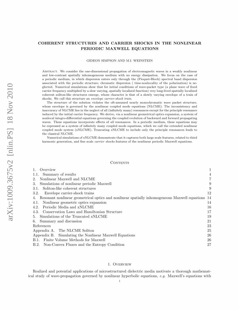
Figure 1. A wavepacket (real part, <E0(z), of complex field) with carrier wave lengthequal twice that of the waveguide refractive index (n(z)).
The term gap soliton is used due to frequency of the gap soliton envelope lying in the spectral gap of thelinearized system.
Physical predictions of gap solitons are based on explicit solutions of nonlinear coupled mode equations(NLCME), given below in (2.9). NLCME has been formally derived in, for example, [4] from (1.4); see alsothe discussion in Section 2. Rigorous derivations of NLCME, from models with appropriate dispersion havebeen presented for the anharmonic Maxwell-Lorentz equations [11] and other nonlinear dispersive equations;see e.g. [12, 34,35,40,41].
Within the approximation of a small amplitude wave field as a wave-packet with slowly varying envelopeand single carrier frequency, propagating through a low contrast periodic structure near the Bragg resonance( see scaling in Figure 1) ), NLCME is argued to govern the principle forward and backward slowly varyingenvelopes of carrier waves; see [4] and references therein.
As discussed in [11] and in section 2, if the only source of dispersion is the spatial dispersion of theperiodic medium (e.g. negligible chromatic dispersion) for weakly nonlinear waves in low contrast media allnonlinearity-generated harmonics are resonant and therefore all mode amplitudes are coupled at leading order.The correct mathematical description would appear to require infinitely many interacting modes. Thus, theclassical NLCME are not a mathematically consistent approximation. NLCME may however be satisfactoryphysical description, for some purposes.t Indeed, the soliton wave form prediction based on NLCME appearsto describe some features of experiment. 2
Question 2: Do nonlinear periodic hyperbolic systems have stable coherent structures, and can one developa mathematical theory? How are the classical NLCME related to this theory? See the discussion in section6.
2Physicists argue in two ways that the coupling to higher harmonics is argued to be negligible : (i) The material systemsconsidered are dissipative at higher wave numbers. Higher wave numbers are damped and therefore these mode amplitudes canbe ignored, and (ii) Chromatic dispersion (arising due to the finite time response of the medium to the field) causes nonlinearly
generated harmonics to be off-resonance. Therefore, an initial condition exciting the principle modes will not appreciable excitehigher harmonics. These rationales are somewhat ad hoc since the precise damping mechanisms are not well-understood andchromatic dispersion is a much weaker effect than photonic band dispersion for weak periodic structures.
3
−500 −400 −300 −200 −100 0 100 200 300 400 500−2
−1.5
−1
−0.5
0
0.5
1
1.5
2t = 198
z
E
(a)
−500 −400 −300 −200 −100 0 100 200 300 400 500−2
−1.5
−1
−0.5
0
0.5
1
1.5
2
z
E
t = 198
(b)
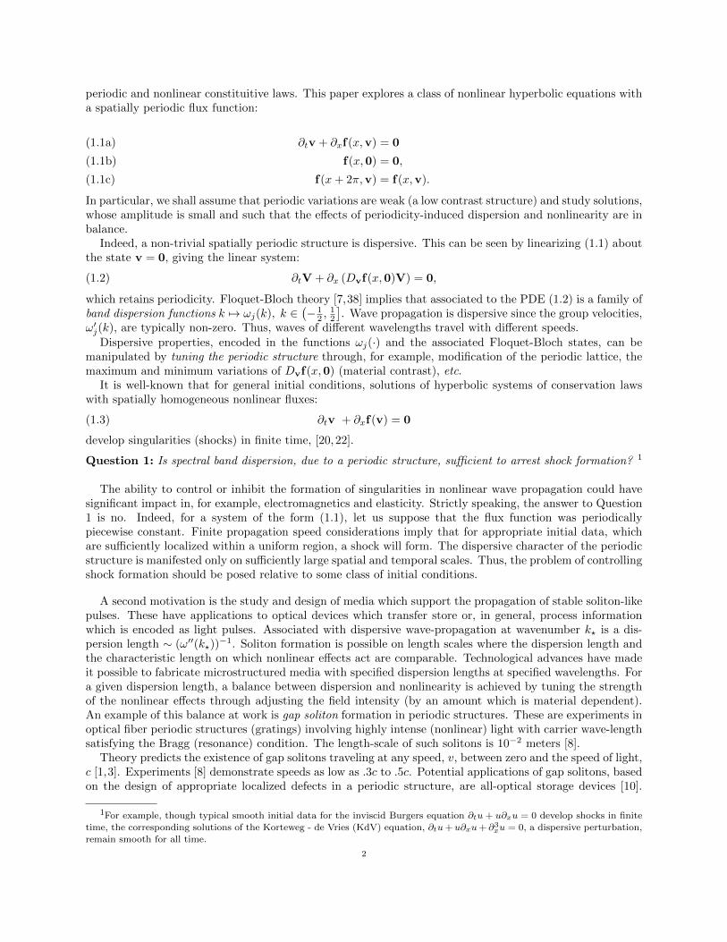
Figure 2. On the left is a simulation of the Maxwell equations. On the right is thesimulation of a truncated asymptotic system, resolving the first and third harmonics. Bothsimulations were initiated with the same initial conditions. The two side pulses about themain wave appear to be the result of third harmonic generation.
In this article we report on progress on Questions 1 and 2 in the context of the one-dimensional, nonlinearMaxwell equations governing the electric (E) and magnetic (B) fields:
∂tD = ∂zB,(1.4a)
∂tB = ∂zE.(1.4b)
with constitutive law
D = ε(z, E) E ≡(n2(z) + χE2
)E(1.5)
n(z) = n0 + εN(z)(1.6)
n(z) is a linear refractive index, consisting of a nonzero background average part, n0, and a fluctuating (e.g.periodic) part εN(z). The nonlinear term χE2 is the nonlinear refractive index, arising from the Kerr effect;in regions of high intensity the refractive index is higher. The consituitive law (1.5), prescribes D as a alocal function of E. Thus chromatic dispersion, which arises due a time-nonlocal relation between D and Ehas been neglected. For simplicity, we assume n0 = 1, which can be arranged by a simple scaling.
1.1. Summary of results.
(1) In section 3 we present numerical simulations of the nonlinear periodic Maxwell equations, (1.4), forinitial data obtained from the explicit NLCME soliton. Under this time-evolution there is robustspatially localized structure on the scale of the NLCME soliton envelope. The persistence of alocalized structure and speed of propagation are consistent with that of the NLCME soliton. Thereis, however, a deviation from the NLCME soliton related to third harmonic generation; these are thetwo accessory pulses around the principle wave in Figure 2 (a).
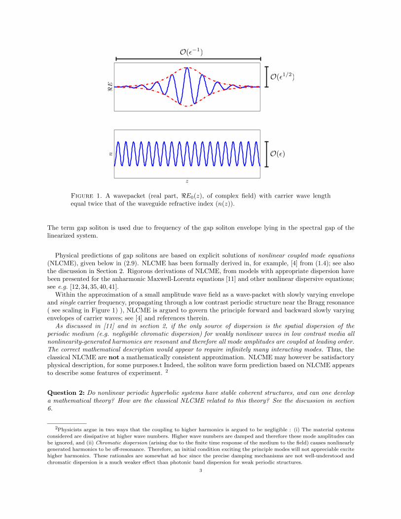
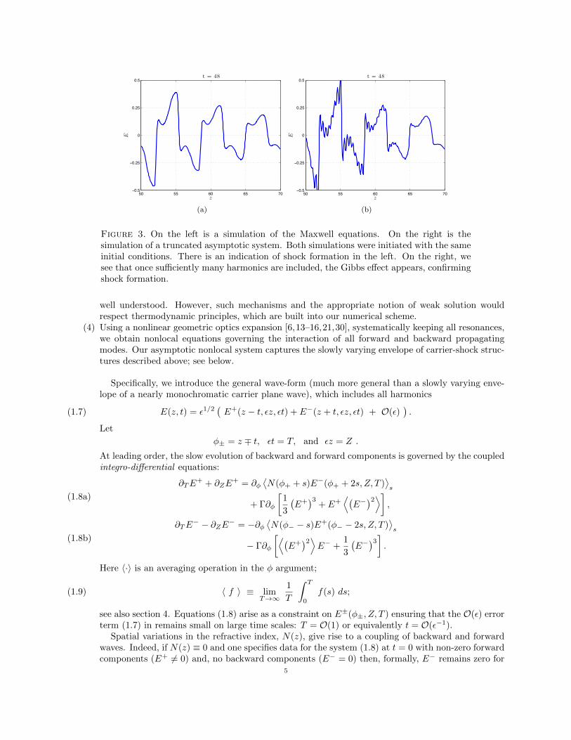
(2) On the microscopic scale of the carrier there is nonlinear steepening and shock formation. Therefore,the solution does not evolve as a slowly varying envelope of a single frequency carrier wave. The long-lived and spatially localized coherent structure which emerges has the character of a slowly varyingenvelope of a train of shocks. We call this an envelope carrier-shock train. Figure 3 illustrates theshock-like small spatial scale behavior under slowly varying envelope.
(3) Numerical solution of the nonlinear Maxwell equation (1.4) is non-trivial due to the cubic nonlin-earity. As a hyperbolic system, it is neither genuinely nonlinear nor linearly degenerate [23, 29, 44].To solve by finite volume methods, as we do, an explicit solution of the Riemann problem must beconstructed. Details of this are given in Appendix B.
The appropriate entropy condition could, in principle be derived from physical regularizationmechanisms, which play the role of viscosity in gas dynamics. However, these mechanisms are not
4
50 55 60 65 70−0.5
−0.25
0
0.25
0.5t = 48
z
E
(a)
50 55 60 65 70−0.5
−0.25
0
0.25
0.5
z
E
t = 48
(b)
Figure 3. On the left is a simulation of the Maxwell equations. On the right is thesimulation of a truncated asymptotic system. Both simulations were initiated with the sameinitial conditions. There is an indication of shock formation in the left. On the right, wesee that once sufficiently many harmonics are included, the Gibbs effect appears, confirmingshock formation.
well understood. However, such mechanisms and the appropriate notion of weak solution wouldrespect thermodynamic principles, which are built into our numerical scheme.
(4) Using a nonlinear geometric optics expansion [6,13–16,21,30], systematically keeping all resonances,we obtain nonlocal equations governing the interaction of all forward and backward propagatingmodes. Our asymptotic nonlocal system captures the slowly varying envelope of carrier-shock struc-tures described above; see below.
Specifically, we introduce the general wave-form (much more general than a slowly varying enve-lope of a nearly monochromatic carrier plane wave), which includes all harmonics
(1.7) E(z, t) = ε1/2(E+(z − t, εz, εt) + E−(z + t, εz, εt) + O(ε)
).
Let
φ± = z ∓ t, εt = T, and εz = Z .
At leading order, the slow evolution of backward and forward components is governed by the coupledintegro-differential equations:
∂TE+ + ∂ZE
+ = ∂φ⟨N(φ+ + s)E−(φ+ + 2s, Z, T )
⟩s
+ Γ∂φ
[1
3
(E+)3
+ E+⟨(E−)2⟩]
,(1.8a)
∂TE− − ∂ZE− = −∂φ
⟨N(φ− − s)E+(φ− − 2s, Z, T )
⟩s
− Γ∂φ
[⟨(E+)2⟩
E− +1
3
(E−)3]
.(1.8b)
Here 〈·〉 is an averaging operation in the φ argument;
(1.9) 〈 f 〉 ≡ limT→∞
1
T
∫ T
0
f(s) ds;
see also section 4. Equations (1.8) arise as a constraint on E±(φ±, Z, T ) ensuring that the O(ε) errorterm (1.7) in remains small on large time scales: T = O(1) or equivalently t = O(ε−1).
Spatial variations in the refractive index, N(z), give rise to a coupling of backward and forwardwaves. Indeed, if N(z) ≡ 0 and one specifies data for the system (1.8) at t = 0 with non-zero forwardcomponents (E+ 6= 0) and, no backward components (E− = 0) then, formally, E− remains zero for
5

20 40 60 80 100 120 140 160 180 20010
−6
10−5
10−4
10−3
10−2
10−1
100
101
t
e1e3e5e7e9e11e13e15Total Eng.
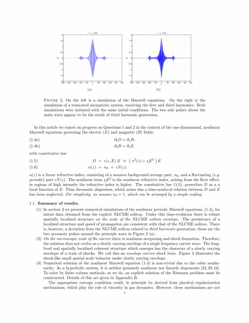
Figure 4. Truncating (1.10) to odd harmonics |p| ≤ 16, we simulate the initial valueproblem an NLCME soliton in the first harmonic, and the others zero. The above timeseries of the energy associated with each harmonic, ep, shows that most of the energycontinues to reside in the first harmonic.
all time, i.e. no backward waves are generated. Continuing with this assumption of N = 0 andE−0 = 0, if we let V (φ, T ) = E+(φ,Z0 − T, T ), with Z0 arbitrary, then V satisfies
∂TV = Γ3 ∂φ(V 3).
This generalized Burger’s equation will gives rise to a finite time singularity. We revisit this obser-vation in the discussion, section 6, when considering how singularities might appear when the linearcoupling between backwards and forwards waves is restored, N 6= 0.
(5) The nonlocal equations may also be written as an infinite system of coupled mode equations. In thecase where E± is 2π− periodic in φ±, the integro-differential equation (1.8) reduces to an infinitesystem of coupled mode equations for the Fourier coefficients
{E±p (Z, T ) : p ∈ Z
}:
∂TE+p + ∂ZE
+p = ipN2pE
−p + ip
Γ
3
[∑E+q E
+r E
+p−q−r
+3(∑∣∣E−q ∣∣2)E+
p
],
(1.10a)
∂TE−p − ∂ZE−p = ipN2pE
+p + ip
Γ
3
[∑E−q E
−r E−p−q−r
+3(∑∣∣E+
q
∣∣2)E−p ] .(1.10b)
We call this system the extended nonlinear coupled mode equations (xNLCME). xNLCME reducesto the classical NLCME if we neglect higher harmonics.
(6) Simulations of successively higher dimensional mode truncations of (1.10) show improved resolutionof the carrier shocks under a slowly varying envelope, whose scale is captured by a comparatively loworder truncation. Indeed, Figure 2 (b) shows that inclusion of the third harmonic in the asymptoticsystem resolves the large scale feature, while inclusion of additional harmonics in Figure 3 (b) showsthe Gibbs effect, expected for a finite Fourier representation of a discontinuous function. Thisdemonstrates that our asymptotic analysis leads to equations capturing the essential features ofnonlinear Maxwell. However, if we consider how energy, initially only in the first harmonic, isredistributed in time, we see in Figure 4 that most of the energy persists in the first harmonic. Thisreflects the partial success of NLCME as a model for periodic nonlinear Maxwell.
areRelation to previous work: Some of the earliest examinations on optical shocks can be found in Rosen, [39],and, DeMartini et al. [5]. In these works, the authors applied the method of characteristics to a unidicretional
6
model. Kinsler and Kinsler et al. have continued to examine this problem, and have developed an algorithmfor detecting the onset of shock formation, [18, 19]. Carrier shocks were also examined by Flesch, Moloney,& Mlejnek, [9], for spatially homogeneous Maxwell system with chromatic dispersion, modeled via a time-nonlocal Lorentzian polarization response. Ranka, Windeler, & Stentz have found experimental evidence ofoptical shocks, [37]. In their work, a monochromatic pulse with sufficient power steepened and generated abroadband optical continuum.
Coherent structures in nonlinear and periodic media have also been studied by LeVeque, LeVeque &Yong, and Ketcheson [17, 25, 26] in a model for heterogeneous nonlinear elastic media. They consideredorder one solutions in high contrast, rapidly varying, periodic structures. Their simulations yielded localizedstructures on the scale of many periods with oscillations on the scale of the period. For piecewise constant(discontinuous) periodic structures, they have a discontinuous carrier shock-like character on the scale ofthe period, though this is due to discontinuities in the medium, the fluxes remain continuous. A two-scale (homogenization) expansion yields a nonlinear dispersive equation, with solitary waves, similar to thecomputed solution envelope. In their physical regime, the variations in the properties of the media and thenonlinearity are O(1). In contrast, we consider an asymptotic regime where the constrast of the periodicstructure and nonlinearity are of the same order, O(ε). Furthermore, the initial condition has two scales(envelope and carrier scales), where the carrier wave length is of the same order, indeed in resonance with,the periodic structure. These different scalings lead to different asymptotic descriptions. An early exampleof the interactions between nonlinearity and a periodic structure was in atmospheric science, studied byMajda et al., [31]. In this work, a model of the interaction of equatorial waves with topography gives rise tononsmooth profiles (in this case, solitary waves with corner singularities).
Finally, systems of coupled modes have also been examined in prior works, though the work is typicallylimited two just two harmonics, such as a first and second harmonic system or a first and third harmonic sys-tem. Such a system was studied by Tasgal, Band, & Malomed [46], who were able to find stable polychromaticsolitons in a first and third harmonic system.
An outline of this paper is as follows. In Section 2, we review how NLCME arises as an approximation ofnonlinear Maxwell. Results of Maxwell Simulations, showing the coherent structures and shocks, are givenpresented in Section 3. We then present our derivation of xNLCME in Section 4, followed by simulations ofthis system in Section 5. We discuss all of these results in Section 6.
Acknowledgements: The authors would like to thank R.R. Rosales for discussions during the earlystages of this work on the use nonlinear geometrical optics. We also thank M. Pugh, D. Ketcheson, R.J.LeVeque, and C. Sulem for helpful discussions. GS was supported in part by NSF-IGERT grant DGE-02-21041, NSF-CMG grant DMS-05-30853, and NSERC. MIW was supported in part by NSF grants DMS-07-07850 and DMS-10-08855. MIW would also like to acknowledge the hospitality of the Courant Institute ofMathematical Sciences, where he was on sabbatical during the preparation of this article.
2. Nonlinear Maxwell and NLCME
In this section we briefly review how NLCME arises from nonlinear Maxwell with a periodically varyingindex of refraction. We also identify the mathematical inconsistency of NLCME as a description of thewave-envelope.
First, we write the nonlinear Maxwell equation (1.4) as
(2.1) ∂2t
(n(z)2E + χE3
)= ∂2
zE
with index of refraction
(2.2) n(z) = 1 + εN(z), 0 < ε� 1,
where N(z) is 2π periodic with mean zero and Fourier series:
(2.3) N(z) =∑
p∈Z\{0}Npe
ipz.
We shall seek solutions which incorporate (i) slow variations in time and space, due to the weak modulationabout a constant refractive index; (ii) a scaling of the wave-field which seeks solutions in which the effects
7
of dispersion and nonlinearity are in balance:
(2.4) Eε(z, t) = ε12 Eε(z, t;Z, T ), Z = εz, T = εt.
Rewriting (2.1) in terms of new variables dependent Eε and independent (z, t, Z, T ) variables, we obtain:(∂2t − ∂2
z
)Eε + ε
(2∂t∂TEε − 2∂z∂ZEε + 2N(z)Eε + χ (Eε)3
)+ O(ε3) = 0.
Formally expanding Eε as
Eε(z, t, Z, T ) = E0(z, t, Z, T ) + ε E1(z, t, Z, T ) + . . .
we obtain the following hierarchy for Ej(z, t, Z, T ), j ≥ 0:
O(ε0)(∂2t − ∂2
z
)E0 = 0
O(ε1)(∂2t − ∂2
z
)E1 = −2∂t∂TE0 + 2∂z∂ZE0 − 2N(z)E0 − χ (E0)
3
...
O(εj)(∂2t − ∂2
z
)Ej = expressions in terms of El, 0 ≤ l ≤ j − 1
...
(2.5)
Solving the O(ε0) equation yields:
(2.6) E0(z, t, Z, T ) = E+(Z, T )ei(z−t) + E−(Z, T )e−i(z+t) + c.c.
Thus, the leading order consists of backward and forward propagating waves, modulated by the slow envelopeamplitude functions E±(Z, T ), which are to be determined.
Substitution of (2.6) into the O(ε1) equation for E1 yields the equation:(∂2t − ∂2
z
)E1
=[2i∂TE+ − 2i∂ZE+ − 2N2E− − 3χ
(∣∣E+∣∣2 + 2
∣∣E−∣∣2) E+]ei(z−t)
+[2i∂TE− − 2i∂ZE+ − 2N2E+ − 3χ
(∣∣E−∣∣2 + 2∣∣E+
∣∣2) E−] e−i(z+t)+(E+)3e3i(z−t) +
(E−)3e−3i(z+t) + c.c.+ non-resonant terms
(2.7)
We have used that N0 = 0 and
N(z)(E+ei(z−t) + E−e−i(z+t))= N−2E+e−i(z+t) +N2E−ei(z−t) + c.c.+ non-resonant terms.
(2.8)
Each term, explicitly written on the right hand side of (2.7), is resonant with the kernel of(∂2t − ∂2
z
). It
follows that the coefficients of all harmonic plane waves: e±iq(z−t) and e±iq(z+t), q ∈ Z must vanish for E1to be bounded in t.
The vanishing of the coefficients of ei(z−t) and e−i(z+t) yields the nonlinear coupled mode equations(NLCME):
∂TE+ + ∂ZE+ = iN2E− + iΓ(∣∣E+
∣∣2 + 2∣∣E−∣∣2) E+,(2.9a)
∂TE− − ∂ZE− = iN2E+ + iΓ(∣∣E−∣∣2 + 2
∣∣E+∣∣2) E−,(2.9b)
where Γ ≡ 32χ and N2 = N−2. The initial value problem for (2.9) is well-posed [11]. NLCME also has
explicit family of gap-soliton solutions; see Appendix A.However, requiring E± to satisfy (2.9) removes only the lowest harmonic resonances. This is the approxi-
mation invoked in the physics literature; see the survey [4] and references cited therein.Note however that the remaining explicitly displayed terms on the right hand side of (2.7) are resonant as
well and induce linear in time growth. If we choose to remove the resonant terms proportional to e3i(z−t) ande−3i(z+t) by including slow modulations of these plane waves at O(ε0), nonlinearity and parametric forcingthrough N(z) will generate yet other resonant harmonics.
8
A leading order solution which does not generate resonant terms at higher order must contain all harmon-ics. Thus, NLCME is mathematically inconsistent. In section 4 we derive an integro-differential equation,which consistently incorporates all resonances. As seen from our numerical and asymptotic studies, this non-local nonlinear geometrical optics equation more accurately capture features on both small and large spatialscales, e.g. changes in the envelope due to higher harmonic generation, as well as carrier shock formation.
3. Simulations of nonlinear periodic Maxwell
In this section we discuss the results of numerical simulations, based on the algorithms of Appendix B, ofthe nonlinear and periodic Maxwell equations (2.1).
• In section 3.1 we show that for Cauchy initial data derived from the classical NLCME soliton, thereevolve spatially localized soliton-like states which persist on long time scales. We discuss aspects ofthe large scale (envelope) structure of such states, which are consistent with the NLCME soliton, aswell as significant deviations.
• In section 3.2 we show that smoothness breaks down in finite time. In particular, we observe shockformation on the fast spatial scale of the carrier wave, while a slowly varying envelope evolvessmoothly.
We begin by expressing (2.1) as a first order system:
(3.1) ∂t
(n(z)2E + χE3
B
)+ ∂z
(−B−E
)= 0.
We introduce the scaling (E,B,D)T = ε1/2(E, B, D), and expressing the equations in terms of the variables:
(D, B) coordinates. Dropping tildes, this is
(3.2) ∂t
(DB
)+ ∂z
(−B
−E(D, z)
)= 0.
where E(D, z) is the unique real solution of
(3.3) D = n(z)2E + εχE3
3.1. Soliton-like coherent structures. As is well known [1,3] NLCME has spatially localized gap solitonsolutions. We use the analytical expression for the gap soliton to generate Cauchy initial data, E(z, 0), ∂tE(z, 0)for (2.1) and numerically simulate the evolution.
Using (2.6) and the leading order approximation for the magnetic field B±1 = ∓E±1 , NLCME soliton data(see (A.1) in Appendix A) can be seeded into Maxwell using
E = E+(εz, εt)ei(z−t) + E−(εz, εt)e−i(z+t) + c.c.,(3.4a)
B = −E+(εz, εt)ei(z−t) + E+(εz, εt)ei(z−t) + c.c.(3.4b)
We obtain D via (3.3) and evaluate at t = 0 to get the initial condition.For a spatially varying index of refraction, we take
(3.5) N(z) = 4π cos(2z), i .e. N2 = N−2 = 2
π , Np = 0, |p| 6= 2,
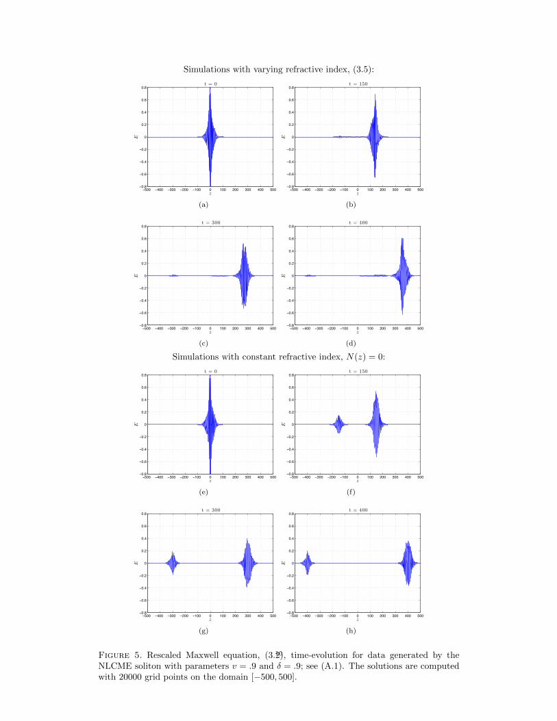
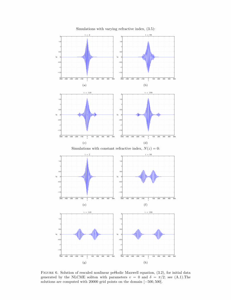
ε = 0.0625, and χ = 1 (Γ = 32 ). The results of our simulations appear in a - d of Figures 5 and 6. While there
is attenuation in amplitude and some dispersive spreading of energy, the solution remains spatially localizedover long time intervals. Not only is there a persistence of the localization (with the periodic medium), butalso there is good pointwise agreement with the NLCME approximation; see Figure 7.
Frames e - h of Figures 5 and 6 display the corresponding results in the absence of a periodic structure,i.e. N(z) ≡ 0. The delocalization, dispersive spreading and attenuation of the wave amplitude is greatlyenhanced. To understand this heuristically, note that a gap soliton is a localized state whose frequency lies inthe spectral gap of the linearized PDE at the zero solution. A focusing nonlinearity adds a (self-consistent)potential well, creating a (nonlinear) defect mode with frequency lying in this spectral gap. If N(z) ≡ 0 thenthe linearization at the zero state has no spectral gap. Thus, a oscillating with the gap soliton frequencywould couple to radiation modes and dispersively spread and attenuate. This mechanism is discussed, forexample, in [45].
9
Simulations with varying refractive index, (3.5):
−500 −400 −300 −200 −100 0 100 200 300 400 500−0.8
−0.6
−0.4
−0.2
0
0.2
0.4
0.6
0.8t = 0
z
E
(a)
−500 −400 −300 −200 −100 0 100 200 300 400 500−0.8
−0.6
−0.4
−0.2
0
0.2
0.4
0.6
0.8t = 150
z
E
(b)
−500 −400 −300 −200 −100 0 100 200 300 400 500−0.8
−0.6
−0.4
−0.2
0
0.2
0.4
0.6
0.8t = 300
z
E
(c)
−500 −400 −300 −200 −100 0 100 200 300 400 500−0.8
−0.6
−0.4
−0.2
0
0.2
0.4
0.6
0.8t = 400
z
E
(d)
Simulations with constant refractive index, N(z) = 0:
−500 −400 −300 −200 −100 0 100 200 300 400 500−0.8
−0.6
−0.4
−0.2
0
0.2
0.4
0.6
0.8t = 0
z
E
(e)
−500 −400 −300 −200 −100 0 100 200 300 400 500−0.8
−0.6
−0.4
−0.2
0
0.2
0.4
0.6
0.8t = 150
z
E
(f)
−500 −400 −300 −200 −100 0 100 200 300 400 500−0.8
−0.6
−0.4
−0.2
0
0.2
0.4
0.6
0.8t = 300
z
E
(g)
−500 −400 −300 −200 −100 0 100 200 300 400 500−0.8
−0.6
−0.4
−0.2
0
0.2
0.4
0.6
0.8t = 400
z
E
(h)
Figure 5. Rescaled Maxwell equation, (3.2), time-evolution for data generated by theNLCME soliton with parameters v = .9 and δ = .9; see (A.1). The solutions are computedwith 20000 grid points on the domain [−500, 500].
10
Simulations with varying refractive index, (3.5):
−500 −400 −300 −200 −100 0 100 200 300 400 500−2
−1.5
−1
−0.5
0
0.5
1
1.5
2t = 2
z
E
(a)
−500 −400 −300 −200 −100 0 100 200 300 400 500−2
−1.5
−1
−0.5
0
0.5
1
1.5
2t = 98
z
E
(b)
−500 −400 −300 −200 −100 0 100 200 300 400 500−2
−1.5
−1
−0.5
0
0.5
1
1.5
2t = 148
z
E
(c)
−500 −400 −300 −200 −100 0 100 200 300 400 500−2
−1.5
−1
−0.5
0
0.5
1
1.5
2t = 198
z
E
(d)
Simulations with constant refractive index, N(z) = 0:
−500 −400 −300 −200 −100 0 100 200 300 400 500−2
−1.5
−1
−0.5
0
0.5
1
1.5
2t = 2
z
E
(e)
−500 −400 −300 −200 −100 0 100 200 300 400 500−2
−1.5
−1
−0.5
0
0.5
1
1.5
2t = 98
z
E
(f)
−500 −400 −300 −200 −100 0 100 200 300 400 500−2
−1.5
−1
−0.5
0
0.5
1
1.5
2t = 148
z
E
(g)
−500 −400 −300 −200 −100 0 100 200 300 400 500−2
−1.5
−1
−0.5
0
0.5
1
1.5
2t = 198
z
E
(h)
Figure 6. Solution of rescaled nonlinear periodic Maxwell equation, (3.2), for initial datagenerated by the NLCME soliton with parameters v = 0 and δ = π/2; see (A.1).Thesolutions are computed with 20000 grid points on the domain [−500, 500].
11
(a) (b)
(c) (d)
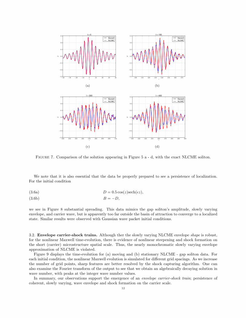
Figure 7. Comparison of the solution appearing in Figure 5 a - d, with the exact NLCME soliton.
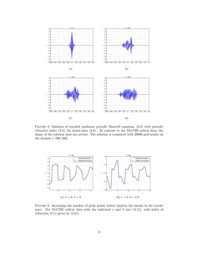
We note that it is also essential that the data be properly prepared to see a persistence of localization.For the initial condition
D = 0.5 cos(z)sech(εz),(3.6a)
B = −D,(3.6b)
we see in Figure 8 substantial spreading. This data mimics the gap soliton’s amplitude, slowly varyingenvelope, and carrier wave, but is apparently too far outside the basin of attraction to converge to a localizedstate. Similar results were observed with Gaussian wave packet initial conditions.
3.2. Envelope carrier-shock trains. Although ther the slowly varying NLCME envelope shape is robust,for the nonlinear Maxwell time-evolution, there is evidence of nonlinear steepening and shock formation onthe short (carrier) microstructure spatial scale. Thus, the nearly monochromatic slowly varying envelopeapproximation of NLCME is violated.
Figure 9 displays the time-evolution for (a) moving and (b) stationary NLCME - gap soliton data. Foreach initial condition, the nonlinear Maxwell evolution is simulated for different grid spacings. As we increasethe number of grid points, sharp features are better resolved by the shock capturing algorithm. One canalso examine the Fourier transform of the output to see that we obtain an algebraically decaying solution inwave number, with peaks at the integer wave number values.
In summary, our observations support the emergence of an envelope carrier-shock train; persistence ofcoherent, slowly varying, wave envelope and shock formation on the carrier scale.
12
−500 −400 −300 −200 −100 0 100 200 300 400 500z
−0.6
−0.5
−0.4
−0.3
−0.2
−0.1
0.0
0.1
0.2
0.3
0.4
0.5
0.6
E
t = 0
(a)
−500 −400 −300 −200 −100 0 100 200 300 400 500z
−0.6
−0.5
−0.4
−0.3
−0.2
−0.1
0.0
0.1
0.2
0.3
0.4
0.5
0.6
E
t = 100
(b)
−500 −400 −300 −200 −100 0 100 200 300 400 500z
−0.6
−0.5
−0.4
−0.3
−0.2
−0.1
0.0
0.1
0.2
0.3
0.4
0.5
0.6
E
t = 150
(c)
−500 −400 −300 −200 −100 0 100 200 300 400 500z
−0.6
−0.5
−0.4
−0.3
−0.2
−0.1
0.0
0.1
0.2
0.3
0.4
0.5
0.6
E
t = 200
(d)
Figure 8. Solution of rescaled nonlinear periodic Maxwell equation, (3.2) with periodicrefractive index (3.5), for initial data (3.6) . In contrast to the NLCME soliton data, theshape of the solution does not persist. The solution is computed with 20000 grid points onthe domain [−500, 500].
(a) v = .9, δ = .9 (b) v = 0, δ = π/2
Figure 9. Increasing the number of grids points better resolves the shocks in the carrierwave. For NLCME soliton data with the indicated v and δ (see (A.1)), with index ofrefraction N(z) given by (3.5)).
13
4. Resonant nonlinear geometrical optics and nonlinear spatially inhomogeneousMaxwell equations
In this section we derive a system of equations, which incorporates all wave-resonances and which ournumerical simulations show, captures the key features of the nonlinear Maxwell time-evolution, in par-ticular, the presence of robust envelope carrier-shock train solutions. We derive this system, for generalnon-homogeneous media, using a nonlinear geometrical optics expansion; see, for example, [13, 14, 30]. Theequations obtained are the general integro-differential equations (1.8). In the case of a periodic medium,they reduce to an infinite set of local equations, which we call the extended nonlinear coupled mode equations(xNLCME). If, in xNLCME, we neglect all but principle resonances, xNLCME reduces to NLCME.
As we shall see, in our numerical simulations of increasing high dimensional truncations of xNLCME (sec-tion 5), this theory appears to accommodate the observed carrier shocks and large scale coherent structures.
4.1. Nonlinear geometric optics expansion. In contrast to the ansatz of Section 2, we assume the moregeneral form
(4.1) u(z, t) = u(0)(z, t, Z, T ) + εu(1)(z, t, Z, T ) + ε2u(2)(z, t, Z, T ) + . . . .
where u = (E,B)T and Z = εz, T = εt. Inserting (4.1) into (3.2), (3.3), the first order system
∂t
(n(z)2E + εχE3
B
)+ ∂z
(−B−E
)= 0.
we expand to get, (∂t +B(0)∂z
)u(0) + ε
[(∂t +B(0)∂z
)u(1) +
(∂T +B(0)∂Z
)u(0)
+A(1)(z,u)∂tu(0)]
= O(ε2)
with matrices
(4.2) B(0) =
(0 −1−1 0
), A(1) =
(2N(z) + 3χE2 0
0 0
)At O(ε0),
(4.3)(∂t +B(0)∂z
)u(0) = 0.
Solving this as the generalized Eigenvalue problem,(B(0) − λI
)r = 0
the solutions are:
(4.4) λ± = ±1, r± =
(1∓1
).
The corresponding left eigenvectors are
(4.5) l± = 12
(1 ∓1
)With this normalization, liA
(0)rj = δi,j . The leading order fields are then
u(0) = E+(φ+, Z, T )r+ + E−(φ−, Z, T )r−,(4.6a)
E(0) = E+(φ+, Z, T ) + E−(φ−, Z, T ),(4.6b)
φ± = z ∓ t.(4.6c)
This expression is much more general than (2.6) used in the derivation of NLCME.At O(ε), the equation is(
∂t +B(0)∂z
)u(1) = −
(∂T +B(0)∂Z
)u(0) −A(1)(z,u(0))∂tu
(0)(4.7)
If we assume
(4.8) u(1)(z, t) = m+(z, t)r+ +m−(z, t)r−,14
and substitute into (4.7), then left multiply by l+ and then by l−, we get the two equations
−(∂tm
+ + ∂zm+)
= ∂TE+ + ∂ZE
+ + l+A(1)(u(0))×(
−∂φ+E+r+ + ∂φ−E
−r−),(4.9)
−(∂tm
− − ∂zm−)
= ∂TE− − ∂ZE− + l−A
(1)(u(0))×(−∂φ+E
+r+ + ∂φ−E−r−
).(4.10)
The last term is the same in both equations,
l±A(1)(u(0))
(−∂φ+E
+r+ + ∂φ−E−r−
)= 1
2
(2N(z) + 3χE(0)2
) (−∂φ+E
+ + ∂φ−E−)
= N(z)(−∂φ+E
+ + ∂φ−E−)
+ 32χ(E+ + E−
)2 (−∂φ+E+ + ∂φ−E
−) .(4.11)
Integration of (4.9) along the characteristic ∂tz+ = 1 from t = 0 to t = L, yields
−(m+(z+(L), L)−m+(z+(0), 0)
)=∫ L
0
∂TE+(Z, T, z+(0)) + ∂ZE
+(Z, T, z+(0))ds
−∫ L
0
N(z+(s))∂φ+E+(Z, T, z+(0))ds
+
∫ L
0
N(z+(s))∂φ−E−(Z, T, z+(s) + s)ds
−∫ L
0
[32χ(E+(Z, T, z+(0))− E−(Z, T, z+(s) + s)
)2×∂φ+
E+(Z, T, z+(0))]ds
+
∫ L
0
[32χ(E+(Z, T, z+(0))− E−(Z, T, z+(s) + s)
)2×∂φ−E
−(Z, T, z+(s) + s)]ds.
(4.12)
Similarly, integration of (4.10) along the characteristic ∂tz− = −1, yields
−(m−(z−(L), L)−m−(z−(0), 0)
)=∫ L
0
∂TE−(Z, T, z+(0))− ∂ZE−(Z, T, z+(0))ds
−∫ L
0
N(z−(s))∂φ+E+(Z, T, z−(s)− s)ds
+
∫ L
0
N(z−(s))∂φ−E−(Z, T, z−(0))ds
−∫ L
0
[32χ(E+(Z, T, z−(s)− s)− E−(Z, T, z−(0))
)2×∂φ+
E+(Z, T, z−(s)− s)]ds
+
∫ L
0
[32χ(E+(Z, T, z−(s)− s)− E−(Z, T, z−(0))
)2×∂φ−E
−(Z, T, z−(0))]ds.
(4.13)
15
Necessary conditions for m± to grow sublinearly in t as t→∞ are the solvability conditions:
∂TE+(Z, T, z+(0)) + ∂ZE
+(Z, T, z+(0)) =
− limL→∞
1
L
∫ L
0
N(z+(s))∂z+(0)E−(Z, T, z+(s) + s)ds
+ limL→∞
1
L
∫ L
0
[32χ(E+(Z, T, z+(0)) + E−(Z, T, z+(s) + s)
)2×∂z+(0)E
+(Z, T, z+(0))]ds,
(4.14a)
(4.14b)
∂TE−(Z, T, z−(0))− ∂ZE−(Z, T, z−(0)) =
limL→∞
1
L
∫ t
0
N(z−(s))∂z−(0)E+(Z, T, z−(s)− s)ds
− limL→∞
1
L
∫ L
0
[32χ(E+(Z, T, z−(s)− s)− E−(Z, T, z−(0))
)2∂z−(0)E
−(Z, T, z−(0))]ds.
(4.14c)
Given (z, t), z+(0) = z − t = φ+ and z−(0) = z + t = φ−. Defining
(4.15) 〈f〉 = limL→∞
1
L
∫ L
0
f(s)ds
the equations may be compactly expressed as:
∂TE+ + ∂ZE
+ = −⟨N(φ+ + s)∂φE
−(φ+ + 2s⟩s
+ 32χ((E+)2
+ 2E+⟨E−⟩
+⟨(E−)2⟩)
∂φE+,
(4.16a)
∂TE− − ∂ZE− =
⟨N(φ− − s)∂φE+(φ− − 2s)
⟩s
− 32χ((E−)2
+ 2E−⟨E+⟩
+⟨(E+)2⟩)
∂φE−.
(4.16b)
It is important to recognize that the arguments of the fields in (4.16a) are φ+ = z − t, Z, and T , while in(4.16b), they are φ− = z + t, Z, and T . As in our derivation of NLCME in Section 2, Γ ≡ 3
2χ. With thisnotation, (4.16) can be rewritten, after an integration by parts, in conservation law form,
∂TE+ + ∂ZE
+ = ∂φ⟨n1(φ+ + s)E−(φ+ + 2s
⟩s
+ Γ∂φ
[1
3
(E+)3
+(E+)2 ⟨
E−⟩
+ E+⟨(E−)2⟩]
,(4.17a)
∂TE− − ∂ZE− = −∂φ
⟨n1(φ− − s)E+(φ− − 2s)
⟩s
− Γ∂φ
[⟨(E+)2⟩
E− +⟨E+⟩ (E−)2
+1
3
(E−)3]
.(4.17b)
Equations (4.17) corresponds to the integro-differential equations of the introduction, if we omit the 〈E±〉terms. Since 〈E±〉 is time-invariant (see section 4.3) by choosing initial conditions for which 〈E±〉 (T = 0) =0, these terms can be dropped from (4.17). Finally, note that (4.16) are applicable to a general heterogeneousdielectric material with the appropriate scalings.
4.2. Periodic Media and xNLCME. We now specialize to the periodic case. Assume now that N(z +2π) = N(z). Then (4.17) is invariant under the discrete translation: φ 7→ φ+ 2π, i.e.
E+(φ,Z, T ) 7→ E+(φ+ 2π, Z, T )(4.18a)
E−(φ,Z, T ) 7→ E−(φ+ 2π, Z, T ) .(4.18b)
Thus, under the assumption of existence and uniqueness of solutions to (4.17), if the initial data are 2π inthe φ argument, then the solutions remain 2π periodic in φ. In the periodic setting, the averaging operator,
16
(4.15), simplifies to
〈f〉 =1
2π
∫ 2π
0
f(s)ds.
We now expand N(z) and E± in Fourier series,
N(z) =∑p∈Z
Npeipz,(4.19)
E±(φ,Z, T ) =∑p
E±p (Z, T )e±ipφ,(4.20)
where Np = N−p and E±p = E±−p since N and E± are real valued. In this case, the system of Fourier
coefficients {E±p (Z, T ) : p ∈ Z} satisfy the infinite system of extended nonlinear coupled mode equations(xNLCME):
∂TE+p + ∂ZE
+p = ipN2pE
−p + ip
Γ
3
[∑q,r
E+q E
+r E
+p−q−r
+3E−0∑q
E+q E
+p−q + 3
(∑q
∣∣E−q ∣∣2)E+p
],
(4.21a)
∂TE−p − ∂ZE−p = ipN2pE
+p + ip
Γ
3
[∑q,r
E−q E−r E−p−q−r
+3E+0
∑q
E−q E−p−q + 3
(∑q
∣∣E+q
∣∣2)E−p].
(4.21b)
4.3. Conservation Laws and Hamiltonian Structure. Equation (4.17), and alternatively (4.21), havetwo conservation laws:
Proposition 4.1. Assume that E± is a sufficiently smooth and sufficiently Z− decaying solution of (4.17)and that {Ep(Z, T )}p∈Z is the corresponding solution of xNLCME. Then,
d
dT
∫ ⟨E+(·, T )
⟩dZ =
d
dT
∫E+
0 (·, T ) dZ = 0(4.22a)
d
dT
∫ ⟨E+(·, T )
⟩dZ =
d
dT
∫E−0 (·, T ) dZ = 0(4.22b)
d
dT
∫ ⟨(E+)2(·, T )
⟩+⟨(E−)2(·, T )
⟩dZ(4.22c)
=d
dT
∑p
∫ ∣∣E+p (·, T )
∣∣2 +∣∣E−p (·, T )
∣∣2 dZ = 0 .(4.22d)
Proof. Setting p = 0 in (4.21),
∂TE+0 + ∂ZE
+0 = 0,
∂TE−0 − ∂ZE−0 = 0.
Integrating in Z establishes the first two conservation laws in terms of the Fourier modes. Integrating (4.20)in φ over [0, 2π) relates 〈E±〉 to E±0 .
17
Multiplying (4.21a) by E+p , summing over p, and adding its complex conjugate,
∑∂T∣∣E+
p
∣∣2 + ∂Z∣∣E+
p
∣∣2 =∑p
ipN2pE−p E
+p +
Γ
3
∑p
ip
[∑q,r
E+q E
+r E
+−pE
+p−q−r
+ 3E−0∑q
E+q E
+p−qE
+−p
+3
(∑q
∣∣E−q ∣∣2) ∣∣E+
p
∣∣2 ]+ c.c.
The quartic terms will all vanish. Consider the first quartic term, and note that∑p,q,r
pE+q E
+r E
+−pE
+p−q−r =
∑k1+k2+k3+k4=0
k1E+k1E+k2E+k3E+k4
=∑
k1+k2+k3+k4=0
k2E+k1E+k2E+k3E+k4
=∑
k1+k2+k3+k4=0
k3E+k1E+k2E+k3E+k4
=∑
k1+k2+k3+k4=0
k4E+k1E+k2E+k3E+k4
(4.23)
Hence, ∑p,q,r
pE+q E
+r E
+−pE
+p−q−r
=1
4
∑k1+k2+k3+k4=0
(k1 + k2 + k3 + k4)E+k1E+k2E+k3E+k4
= 0(4.24)
The second quartic term vanishes using a similar analysis. The last quartic term,
(4.25)∑p
p
(∑q
∣∣E−q ∣∣2)∣∣E+
p
∣∣2will vanish because the p and −p terms will cancel one another. Similar analysis holds for (4.21b), leavingus with the two equations∑
∂T∣∣E+
p
∣∣2 + ∂Z∣∣E+
p
∣∣2 =∑
ipN2pE−p E
+p − ipN2pE
−p E
+p ,(4.26) ∑
∂T∣∣E−p ∣∣2 − ∂Z ∣∣E−p ∣∣2 =
∑ipN2pE
−p E
+p − ipN2pE
−p E
+p .(4.27)
Summing these two, and integrating in Z gives the L2 conservation law. �
To simplify our analysis we assume E±0 are initially zero from here on. The equations reduceto
∂TE+ + ∂ZE
+ = ∂φ⟨N(φ+ + s)E−(φ+ + 2s
⟩s
+ Γ∂φ
[1
3
(E+)3
+ E+⟨(E−)2⟩]
,(4.28a)
∂TE− − ∂ZE− = −∂φ
⟨N(φ− − s)E+(φ− − 2s)
⟩s
− Γ∂φ
[⟨(E+)2⟩
E− +1
3
(E−)3]
.(4.28b)
18
and
∂TE+p + ∂ZE
+p = ipN2pE
−p + ip
Γ
3
[∑E+q E
+r E
+p−q−r
+3(∑∣∣E−q ∣∣2)E+
p
],
(4.29a)
∂TE−p − ∂ZE−p = ipN2pE
+p + ip
Γ
3
[∑E−q E
−r E−p−q−r
+3(∑∣∣E+
q
∣∣2)E−p ] .(4.29b)
These are equations (1.8) and (1.10) from the introduction. Truncating (4.29) to just mode E±±1, recovers
the NLCME, subject to the identification of E± with E±1 .Another time-invariant functional is a consequence of the Hamiltonian structure given in the following
result, which is straightforward to verify:
Proposition 4.2. The system (4.29) is a Hamiltonian system:
(4.30) ∂TE+p = −ip
δH
δE+
p
, ∂TE−p = −ip
δH
δE−p
,
where with time-invariant Hamiltonian
H[E±, E±] =
∫H(·, T )
and Hamiltonian density
H(Z, T ) =i
2
∞∑p1=1
1
p1
(E+p1∂ZE
+p1 − E−p1∂ZE−p1
)−∞∑p1=1
N2p1E+p1E
−p1
− Γ
3
1
2
1
4
∑p1+p2+p3+p4=0
E+p1E
+p2E
+p3E
+p4 + E−p1E
−p2E
−p3E
−p4
− Γ1
2
1
2
(∑p1
∣∣E+p1
∣∣2)(∑p1
∣∣E−p1∣∣2)
+ c.c. .
(4.31)
5. Simulations of the Truncated xNLCME
In this section we simulate truncations of the infinite dimensional xNLCME system, performed pseudo-spectrally with fourth order Runge-Kutta time stepping. These simulations suggest that
• xNLCME has its own localized soliton-like structures which better capture the dynamics of thenonlinear periodic Maxwell equation for our class of initial conditions than NLCME and
• xNLCME has singular solutions, {E±p (Z, T )} with a cascade of energy to higher wave numbers, p.The physical electric field
E(z, t) ≈ ε 12
(E+(z − t, , εz, εt) + E−(z + t, , εz, εt)
)= ε
12
∑p∈Z\0
(E+p (Z, T )eip(Z−T )/ε + E−p (Z, T )e−ip(Z+T )/ε
)+ c.c.
develops a carrier-shock train structure.
As we saw in Section 3.1, particularly Figure 6, though the NLCME soliton data appeared robust, therewas some escape of energy. This can be accounted for in the xNLCME through the inclusion of additionalmodes.
Starting with the same initial conditions, we simulate the NLCME soliton of E±±1 with soliton parametersv = 0 and δ = π
2 , and material parameters
Γ = 1, N±2 = 2π , Nj 6=±2 = 0
19
−500 −400 −300 −200 −100 0 100 200 300 400 500−2
−1.5
−1
−0.5
0
0.5
1
1.5
2
z
E
t = 2
−500 −400 −300 −200 −100 0 100 200 300 400 500−2
−1.5
−1
−0.5
0
0.5
1
1.5
2
z
E
t = 98
−500 −400 −300 −200 −100 0 100 200 300 400 500−2
−1.5
−1
−0.5
0
0.5
1
1.5
2
z
E
t = 148
−500 −400 −300 −200 −100 0 100 200 300 400 500−2
−1.5
−1
−0.5
0
0.5
1
1.5
2
z
E
t = 198
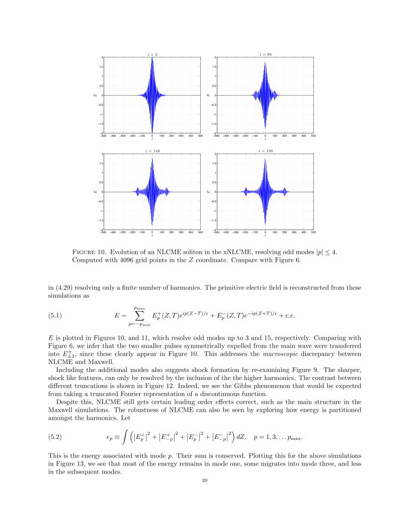
Figure 10. Evolution of an NLCME soliton in the xNLCME, resolving odd modes |p| ≤ 4.Computed with 4096 grid points in the Z coordinate. Compare with Figure 6.
in (4.29) resolving only a finite number of harmonics. The primitive electric field is reconstructed from thesesimulations as
(5.1) E =
pmax∑p=−pmax
E+p (Z, T )eip(Z−T )/ε + E−p (Z, T )e−ip(Z+T )/ε + c.c.
E is plotted in Figures 10, and 11, which resolve odd modes up to 3 and 15, respectively. Comparing withFigure 6, we infer that the two smaller pulses symmetrically expelled from the main wave were transferredinto E±±3, since these clearly appear in Figure 10. This addresses the macroscopic discrepancy betweenNLCME and Maxwell.
Including the additional modes also suggests shock formation by re-examining Figure 9. The sharper,shock like features, can only be resolved by the inclusion of the the higher harmonics. The contrast betweendifferent truncations is shown in Figure 12. Indeed, we see the Gibbs phenomenon that would be expectedfrom taking a truncated Fourier representation of a discontinuous function.
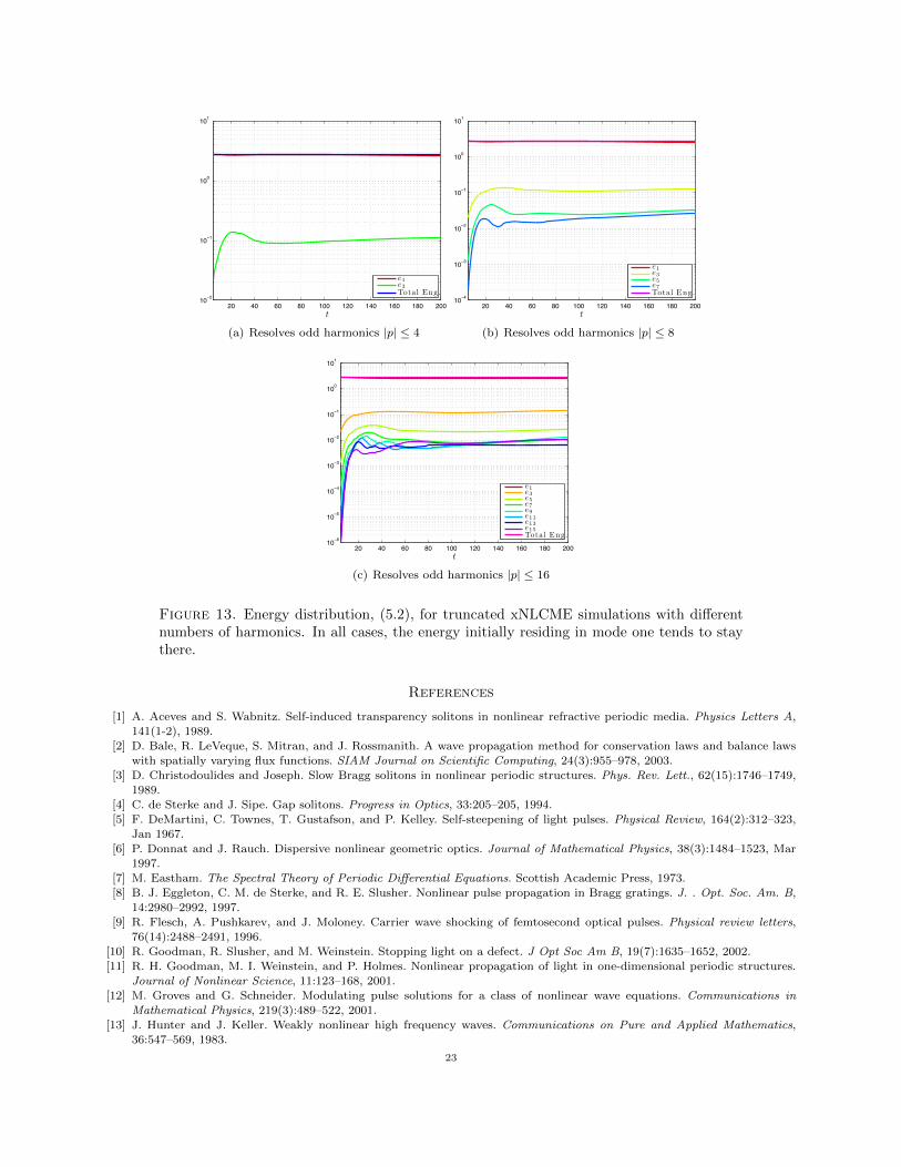
Despite this, NLCME still gets certain leading order effects correct, such as the main structure in theMaxwell simulations. The robustness of NLCME can also be seen by exploring how energy is partitionedamongst the harmonics. Let
(5.2) ep ≡∫ (∣∣E+
p
∣∣2 +∣∣E+−p∣∣2 +
∣∣E−p ∣∣2 +∣∣E−−p∣∣2) dZ, p = 1, 3, . . . pmax.
This is the energy associated with mode p. Their sum is conserved. Plotting this for the above simulationsin Figure 13, we see that most of the energy remains in mode one, some migrates into mode three, and lessin the subsequent modes.
20

−500 −400 −300 −200 −100 0 100 200 300 400 500−2
−1.5
−1
−0.5
0
0.5
1
1.5
2
z
E
t = 2
−500 −400 −300 −200 −100 0 100 200 300 400 500−2
−1.5
−1
−0.5
0
0.5
1
1.5
2
z
E
t = 98
−500 −400 −300 −200 −100 0 100 200 300 400 500−2
−1.5
−1
−0.5
0
0.5
1
1.5
2
z
E
t = 148
−500 −400 −300 −200 −100 0 100 200 300 400 500−2
−1.5
−1
−0.5
0
0.5
1
1.5
2
z
E
t = 198
Figure 11. Evolution of an NLCME solition in the xNLCME, resolving odd modes |p| ≤ 16.Computed with 16384 grid points in the Z coordinate. Compare with Figure 6.
6. Summary and discussion
We first numerically simulated the one-dimensional nonlinear Maxwell equations in the regime of weaknonlinearity, low contrast periodic structure (weak dispersion) with wave-packet data satisfying a Braggresonance condition, i.e. carrier wavelength equal to twice the medium periodicity. We observe strong ev-idence of the emergence of a coherent structure evolving as slowly varying envelope with a carrier-shocktrain. This violates the nearly-monochromatic assumption underlying the classical nonlinear coupled modeequations. We propose our nonlocal integro-differential equations governing coupled forward and backwardwaves, derived via a nonlinear geometrical optics expansion, as the physically correct, mathematically con-sistent description of waves governed by nonlinear Maxwell in a periodic structure with negligible chromatic(nonlocal in time) dispersion. These equations are equivalent to an infinite dimensional system of couple firstorder PDEs, the extended coupled mode system (xNLCME). The electric field, E, obtained from numericalsolution of successively higher truncations of xNLCME converges toward the envelope carrier-shock trainsobserved in direct simulations of the nonlinear Maxwell equations.
Finally we mention that our methods could be applied to study the long time evolution of wave-packettype initial conditions for the problem of quadratically nonlinear elastic media, consider in [17, 25, 26] Weobtain nonlocal equations of resonant nonlinear geometrical optics (or equivalently an infinite family ofnonlinear coupled mode equations), governing interacting forward and backward propagating waves [42]. Adifference between the quadratic and cubic case is that the smallest truncated system that retains nonlinearinteractions contains four modes, p = ±1,±2. Nonlinear effects occur through second harmonic generation,a process well-known in nonlinear optics.Open problems and conjectures: As our simulations show, there is agreement between finite modetruncations of the integro-differential equations and the primitive Maxwell system. Assessing, and provingthe time of validity of this approximation is one upon problem.
21

50 55 60 65 70−0.5
−0.25
0
0.25
0.5
z
E
t = 48
(a) Resolves odd harmonics |p| ≤ 2
50 55 60 65 70−0.5
−0.25
0
0.25
0.5
z
E
t = 48
(b) Resolves odd harmonics |p| ≤ 4
50 55 60 65 70−0.5
−0.25
0
0.25
0.5
z
E
t = 48
(c) Resolves odd harmonics |p| ≤ 8
50 55 60 65 70−0.5
−0.25
0
0.25
0.5
z
E
t = 48
(d) Resolves odd harmonics |p| ≤ 16
Figure 12. Comparison of the features that develop on the scale of the medium in differenttruncations of the equations. Including additional harmonics better captures the shocks seenin Figure 9.
Following up on assessing the time of validity, there is also the question of the time of existence andthe well-posedness of the equations. We expect that solutions of xNLCME for initial data having a finitenumber of nonzero mode amplitudes, e.g. NLCME gap soliton data, will give rise to solutions of xNLCMEthat develop singularities in finite time. The nature of this blowup is expected to occur via a cascadeto high mode amplitudes (higher index, p), corresponding to modes necessary to resolve the carrier shockstructure in the small scale. As we mentioned in the discussion, there is clearly singularity formation whenthe heterogeneity is turned off (N = 0), and either E+ or E− is initially zero. It is an open problem as towhether this particular mechanism for singularity formation will persist when coupling is restored.
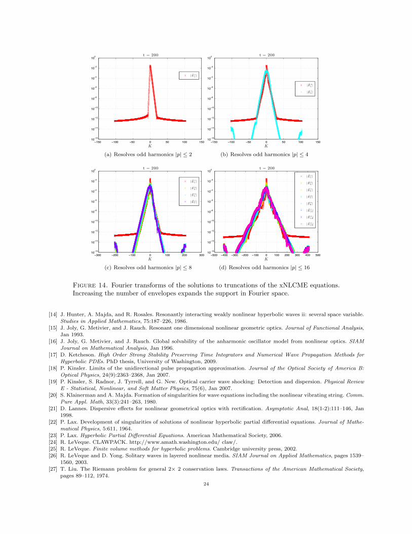
As pointed out in the introduction, the success in modeling experiments with NLCME suggests that,although there is such a (weakly turbulent) cascade, it is only a small part of the optical power that istransferred to high wavenumbers and that this energy contributes mainly to resolving the small-scale shocks.To explore this, one needs to simulate the xNLCME equations with many more harmonics. Plotting theFourier transform (in the Z coordinate) of the simulations in Section 5 in figure 14, we see that the spectralsupport grows as we increase the number of resolved envelopes (the E±p ’s). A related question is whether ornot the primitive Maxwell system, the xNLCME system, or one of its truncations possess genuine coherentstructures. In [46], the authors found such solutions for a first and third harmonic system. This shall befurther explored in the forthcoming publication, [36].
Finally, our computations in Section 3 invoked of a gas-dynamics entropy condition. Such a condition isnecessary to use finite volume methods. Although thermodynamically consistent, we do not know whetherthis is the correct regularizing mechanism of electrodynamics.
22
20 40 60 80 100 120 140 160 180 20010
−2
10−1
100
101
t
e1e3Total Eng.
(a) Resolves odd harmonics |p| ≤ 4
20 40 60 80 100 120 140 160 180 20010
−4
10−3
10−2
10−1
100
101
t
e1e3e5e7Total Eng.
(b) Resolves odd harmonics |p| ≤ 8
20 40 60 80 100 120 140 160 180 20010
−6
10−5
10−4
10−3
10−2
10−1
100
101
t
e1e3e5e7e9e11e13e15Total Eng.
(c) Resolves odd harmonics |p| ≤ 16
Figure 13. Energy distribution, (5.2), for truncated xNLCME simulations with differentnumbers of harmonics. In all cases, the energy initially residing in mode one tends to staythere.
References
[1] A. Aceves and S. Wabnitz. Self-induced transparency solitons in nonlinear refractive periodic media. Physics Letters A,141(1-2), 1989.
[2] D. Bale, R. LeVeque, S. Mitran, and J. Rossmanith. A wave propagation method for conservation laws and balance laws
with spatially varying flux functions. SIAM Journal on Scientific Computing, 24(3):955–978, 2003.[3] D. Christodoulides and Joseph. Slow Bragg solitons in nonlinear periodic structures. Phys. Rev. Lett., 62(15):1746–1749,
1989.
[4] C. de Sterke and J. Sipe. Gap solitons. Progress in Optics, 33:205–205, 1994.[5] F. DeMartini, C. Townes, T. Gustafson, and P. Kelley. Self-steepening of light pulses. Physical Review, 164(2):312–323,
Jan 1967.
[6] P. Donnat and J. Rauch. Dispersive nonlinear geometric optics. Journal of Mathematical Physics, 38(3):1484–1523, Mar1997.
[7] M. Eastham. The Spectral Theory of Periodic Differential Equations. Scottish Academic Press, 1973.
[8] B. J. Eggleton, C. M. de Sterke, and R. E. Slusher. Nonlinear pulse propagation in Bragg gratings. J. . Opt. Soc. Am. B,14:2980–2992, 1997.
[9] R. Flesch, A. Pushkarev, and J. Moloney. Carrier wave shocking of femtosecond optical pulses. Physical review letters,76(14):2488–2491, 1996.
[10] R. Goodman, R. Slusher, and M. Weinstein. Stopping light on a defect. J Opt Soc Am B, 19(7):1635–1652, 2002.[11] R. H. Goodman, M. I. Weinstein, and P. Holmes. Nonlinear propagation of light in one-dimensional periodic structures.
Journal of Nonlinear Science, 11:123–168, 2001.[12] M. Groves and G. Schneider. Modulating pulse solutions for a class of nonlinear wave equations. Communications in
Mathematical Physics, 219(3):489–522, 2001.[13] J. Hunter and J. Keller. Weakly nonlinear high frequency waves. Communications on Pure and Applied Mathematics,
36:547–569, 1983.
23
−150 −100 −50 0 50 100 15010
−16
10−14
10−12
10−10
10−8
10−6
10−4
10−2
100
K
t = 200
| E+1 |
(a) Resolves odd harmonics |p| ≤ 2
−150 −100 −50 0 50 100 15010
−16
10−14
10−12
10−10
10−8
10−6
10−4
10−2
100
K
t = 200
| E+1 |
| E+3 |
(b) Resolves odd harmonics |p| ≤ 4
−300 −200 −100 0 100 200 30010
−16
10−14
10−12
10−10
10−8
10−6
10−4
10−2
100
K
t = 200
| E+1 |
| E+3 |
| E+5 |
| E+7 |
(c) Resolves odd harmonics |p| ≤ 8
−500 −400 −300 −200 −100 0 100 200 300 400 50010
−16
10−14
10−12
10−10
10−8
10−6
10−4
10−2
100
K
t = 200
| E+1 |
| E+3 |
| E+5 |
| E+7 |
| E+9 |
| E+11|
| E+13|
| E+15|
(d) Resolves odd harmonics |p| ≤ 16
Figure 14. Fourier transforms of the solutions to truncations of the xNLCME equations.Increasing the number of envelopes expands the support in Fourier space.
[14] J. Hunter, A. Majda, and R. Rosales. Resonantly interacting weakly nonlinear hyperbolic waves ii: several space variable.
Studies in Applied Mathematics, 75:187–226, 1986.
[15] J. Joly, G. Metivier, and J. Rauch. Resonant one dimensional nonlinear geometric optics. Journal of Functional Analysis,Jan 1993.
[16] J. Joly, G. Metivier, and J. Rauch. Global solvability of the anharmonic oscillator model from nonlinear optics. SIAMJournal on Mathematical Analysis, Jan 1996.
[17] D. Ketcheson. High Order Strong Stability Preserving Time Integrators and Numerical Wave Propagation Methods for
Hyperbolic PDEs. PhD thesis, University of Washington, 2009.
[18] P. Kinsler. Limits of the unidirectional pulse propagation approximation. Journal of the Optical Society of America B:Optical Physics, 24(9):2363–2368, Jan 2007.
[19] P. Kinsler, S. Radnor, J. Tyrrell, and G. New. Optical carrier wave shocking: Detection and dispersion. Physical ReviewE - Statistical, Nonlinear, and Soft Matter Physics, 75(6), Jan 2007.
[20] S. Klainerman and A. Majda. Formation of singularities for wave equations including the nonlinear vibrating string. Comm.
Pure Appl. Math, 33(3):241–263, 1980.[21] D. Lannes. Dispersive effects for nonlinear geometrical optics with rectification. Asymptotic Anal, 18(1-2):111–146, Jan
1998.
[22] P. Lax. Development of singularities of solutions of nonlinear hyperbolic partial differential equations. Journal of Mathe-matical Physics, 5:611, 1964.
[23] P. Lax. Hyperbolic Partial Differential Equations. American Mathematical Society, 2006.
[24] R. LeVeque. CLAWPACK. http://www.amath.washington.edu/ claw/.[25] R. LeVeque. Finite volume methods for hyperbolic problems. Cambridge university press, 2002.
[26] R. LeVeque and D. Yong. Solitary waves in layered nonlinear media. SIAM Journal on Applied Mathematics, pages 1539–
1560, 2003.[27] T. Liu. The Riemann problem for general 2× 2 conservation laws. Transactions of the American Mathematical Society,
pages 89–112, 1974.
24
[28] T. Liu. The Riemann problem for general systems of conservation laws. J. Differential Equations, 18(1):218–234, 1975.[29] T. Liu. Hyperbolic and viscous conservation laws. Society for Industrial Mathematics, 2000.
[30] A. Majda and R. Rosales. Resonantly interacting weakly nonlinear hyperbolic waves i: a single space variable. Studies in
Applied Mathematics, 71:149–179, 1984.[31] A. J. Majda, R. Rosales, E. G. Tabak, and C. Turner. Interaction of large-scale equatorial waves and dispersion of kelvin
waves through topographic resonances. Journal of the Atmospheric Sciences, 56:24, 1999.
[32] S. Muller and A. Voss. The riemann problem for the euler equations with nonconvex and nonsmooth equation of state:construction of wave curves. SIAM Journal on Scientific Computing, 28(2):651–681, 2006.
[33] S. Muller and A. Voss. The Riemann problem for the Euler equations with nonconvex and nonsmooth equation of state:construction of wave curves. SIAM Journal on Scientific Computing, 28:651, 2006.
[34] D. Pelinovsky and G. Schneider. Justification of the coupled-mode approximation for a nonlinear elliptic problem with a
periodic potential. Applicable Analysis, 86(8):1017–1036, 2007.[35] D. Pelinovsky and G. Schneider. Moving gap solitons in periodic potentials. Mathematical Methods in the Applied Sciences,
31(14):1739–1760, 2008.
[36] D. Pelinovsky, G. Simpson, and M. Weinstein. Solitons in the nonlinear maxwell equations. In preparation.[37] J. Ranka, R. Windeler, and A. Stentz. Optical properties of high-delta air-silica microstructure optical fibers. Optics letters,
25(11):796–798, Jan 2000.
[38] M. Reed and B. Simon. Methods of Modern Mathematical Physics IV. Analysis of Operators. Academic Press, 1978.[39] G. Rosen. Electromagnetic shocks and the self-annihilation of intense linearly polarized radiation in an ideal dielectric
material. Physical Review, 139(2A):A539–A543, Jan 1965.
[40] G. Schneider. Nonlinear coupled mode dynamics in hyperbolic and parabolic periodically structured spatially extendedsystems. Asymptotic Analysis, 28(2):163–180, 2001.
[41] G. Schneider and H. Uecker. Existence and stability of modulating pulse solutions in Maxwell’s equations describingnonlinear optics. Zeitschrift fur Angewandte Mathematik und Physik (ZAMP), 54(4):677–712, 2003.
[42] G. Simpson and M. Weinstein. Nonlinear geometrical optics and quadratically nonlinear periodic media. Unpublished
Notes, 2010.[43] D. Sjoberg. On uniqueness and continuity for the quasi-linear, bianisotropic Maxwell equations, using an entropy condition.
Progress In Electromagnetics Research, pages 317–339, 2007.
[44] J. Smoller. Shock waves and reaction-diffusion equations. Springer, 1994.[45] A. Soffer and M. Weinstein. Time dependent resonance theory. Geometric and Functional Analysis (GAFA), 1998.
[46] R. Tasgal, Y. Band, and B. Malomed. Gap solitons in a medium with third-harmonic generation. Physical Review E -
Statistical, Nonlinear, and Soft Matter Physics, 72(1):1–10, Jan 2005.[47] B. Wendroff. The Riemann problem for materials with nonconvex equations of state. I. Isentropic flow. J. Math. Anal.
Appl, 38:454–466, 1972.
[48] B. Wendroff. The Riemann problem for materials with nonconvex equations of state. II. General flow. J. Math. Anal. Appl,38:640–658, 1972.
[49] P. Wesseling and D. Van Der Heul. Uniformly effective numerical methods for hyperbolic systems. Computing, 66(3):249–267, 2001.
[50] P. Wesseling, D. van der Heul, and C. Vuik. Unified methods for computing compressible and incompressible flows. In
Proceedings of ECCOMAS, pages 11–14, 2000.
Appendix A. The NLCME Soliton
Using the notation of [11], the NLCME soliton solution of (2.9) is given by:
E+(Z, T ) = sαeiη
√∣∣∣∣N2
2Γ
∣∣∣∣ 1
∆sin δeisσsech(θ − isδ/2)(A.1a)
E−(Z, T ) = −αeiη
√∣∣∣∣N2
2Γ
∣∣∣∣∆ sin δeisσsech(θ + isδ/2)(A.1b)
θ = γN2 sin δ(Z − vT ), σ = γN2 cos δ(vZ − T )(A.1c)
eiη =
(−e
2θ + e−isδ
e2θ + eisδ
)2v/(3−v2)
(A.1d)
γ = 1/√
1− v2, ∆ =
(1− v1 + v
)1/4
(A.1e)
s = sign(N2Γ), α =
√2(1− v2)
3− v2, κ = κN2(A.1f)
We assume that N2 ∈ R. There are two free parameters, |v| < 1 and δ ∈ R.25
Appendix B. Simulating the Nonlinear Maxwell Equations
In vector notation, the rescaled Maxwell system,(3.2), and constitutive law, (3.3), are expressed as
∂t
(DB
)+ ∂z
(−B
−E(D, z)
)= 0
∂tv + ∂zf(v, z) = 0.
(B.1)
To simulate this system of conservation laws, we employ a shock capturing finite volume scheme with theCLAWPACK software, [24, 25]. Furthermore, we employ the f-wave method to accommodate the spatiallyvarying flux function, [2, 25,26] .
To use finite volume methods we must provide the algorithm with a, possibly approximate, solution of theRiemman problem. This introduces a subtlety as our system has a non-convex flux function. Non-convexfluxes lead to interesting waves, including rightward (or leftward) traveling rarefaction and shockwavesthat are “glued” together. Such waves, sometimes called compound or composite waves, were discussedin [27,28,47,48] and more recently in [33,49,50]. Examples are also give in the texts [25,44].
B.1. Finite Volume Methods for Maxwell. In finite volume numerical methods, at each time step, wemust solve a Riemann problem between adjacent grid cells:
vt + f(v; zj)z = 0 for zj−1/2 < z < zj+1/2,
vt + f(v; zj+1)z = 0 for zj+1/2 < z < zj+3/2,
v(z, t = tn) =
{vnj for zj−1/2 < z < zj+1/2,
vnj+1 for zj+1/2 < z < zj+3/2.
(B.2)
zj+1/2 is the interface between the cell centered at zj and the cell centered at zj+1/2. The fluxes are assumedto be constant in z within each computational cell. We aim to provide an exact solution to the Riemannproblem, in contrast to an approximate solutions such as the Roe average.
In the next few sections, we adopt the notation
vt + fl(v)z = 0 for z < 0
vt + fr(v)z = 0 for z > 0
v(z, 0) =
{vl for z < 0
vr for z > 0
(B.3)
where fl(v) = f(v; zj), fr(v) = f(v; zj+1), and we take zj+1/2 = 0.Given any point v in (D,B) phase space, we construct two, entropy condition (specified below) satisfying,
manifolds W1(v) and W2(v). These define the locus of points that can be joined to v by a left-going wavein the former case and a right-going wave in the latter case. We parameterize them in the D component.Given a state v0, Wj(D;v0) is the parametric curve such that:{(
DWj(D;v0)
), for D ∈ R
}=Wj(v0) for j = 1, 2
Were the medium homogeneous, solving the Riemann corresponds to finding the state v? that is theunique point in W1(vl)
⋂W2(vr). In terms of the parametric curves, this point solves the equation:
(B.4) W2
(Dr;
(D?
W1(D?;vl)
))= Br
As the medium is not homogeneous, we match the flux at the interface. We seek vl? and vr? such that:
W1(D?l ;vl) = B?l(B.5a)
fl(v?l ) = fr(v
?r)(B.5b)
W2(Dr;v?r) = Br(B.5c)
v?l is the the entropy satisfying state immediately to the left of the interface and v?r is the entropy satisfyingstate immediately to the right of the interface.
26
For this problem, the flux matching condition is:
E(D?l ; zl) = E(D?
r ; zr)(B.6a)
B?l = B?r(B.6b)
Defining transfer function, T , that, given zl, zr and a left state D?l , the flux matched displacement is:
(B.7) T (D?l ; zl, zr) = D?
r
With this function, (B.5) becomes
(B.8) W2
(Dr;
(T (D?
l ; zl; zr)W1(D?
l ;vl)
))= Br
D?l is the unknown. Once we have this value, we recover E? and B? allowing us to compute the fluxes.
Subject to the specification of the phase space functions Wj are specified, this is a one-dimensional rootfinding problem.
B.2. Non-Convex Fluxes and the Entropy Condition. It remains to specify the manifolds Wj . Thisrequires an additional, non-trivial, assumption on an entropy condition. While such a condition is readilyapparent in gas dynamics and elasticity, the appropriate condition for Maxwell is non-obvious.
In this work, we employ a diffusive entropy condition, akin to that found in gas dynamics. This wassuggested by Sjoberg [43], as part of an entropy-flux pair involving the Poynting vector. This is also aphysically consistent, as many dielectrics absorb the higher harmonics that would appear as the wave beganto shock.
In constructing the entropy satisfying Wj functions, we closely follow [27, 28, 32, 48] and particularly thep-system example in [47]. Graphically, the Wj functions can be constructed by tracing an appropriate convexhull of E(D; z). Shock waves occur when points are joined by chords, rarefaction waves when points arejoined along E(D; z), and composite waves when convex curve is a combination.
Throughout this section we suppress the z argument, and E′(D) = ∂DE(D, z).Since the flux function is no longer uniformly convex, the Lax entropy condition may not be appropriate.
Instead, Liu entropy condition [27,32] may apply. Recall, that if
(B.9) σ(v0,v) ≡ −E(D) + E(D0)
B −B0
then:
• A shock joining v0 to v1 satisfies the Lax entropy condition if the system is convex and either
λ1(v1) < σ < λ1(v0), σ < 0(B.10a)
λ2(v1) < σ < λ2(v0), σ > 0(B.10b)
where λ1 < 0 < λ2 are the eigenvalues of(0 −1
−E′(D) 0
).
• A shock joining v0 to v1 satisfies the Liu entropy condition if
(B.11) σ(v0,v1) ≤ σ(v0, v)
for all points v between the two points along the shock curve in phase space.
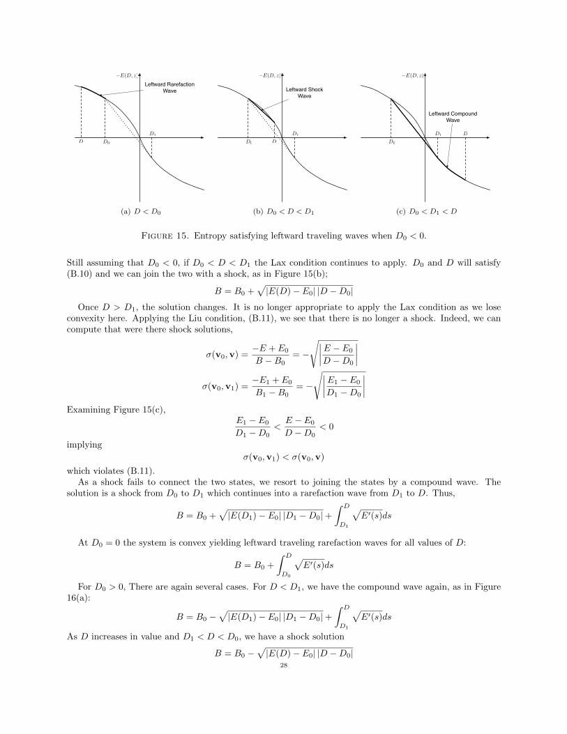
B.2.1. Left Traveling Waves. Given the state u0 = (D0, B0)T , we construct W1(D;u0). Since we have aninflection point in E(D) at D = 0, we dissect all the possible configurations of D0, D and the inflectionpoint. Let D1 be the value of D at which the line tangent to (D1, E(D1)) intercepts (D0, E(D0)).
First, suppose that D < D0 < 0, as in Figure 15(a). In this region, there is no difficulty applying the Laxentropy condition (B.10); there is no shock as
λ1(D) = −√E′(D) < λ1(D0) = −
√E′(D0) < 0
Consequently,
B = B0 +
∫ D
D0
√E′(s)ds
27
D0D
−E(D, z)
Leftward Rarefaction Wave
D1
(a) D < D0
D0 D
−E(D, z)
Leftward Shock Wave
D1
(b) D0 < D < D1
D0
D
−E(D, z)
Leftward Compound Wave
D1
(c) D0 < D1 < D
Figure 15. Entropy satisfying leftward traveling waves when D0 < 0.
Still assuming that D0 < 0, if D0 < D < D1 the Lax condition continues to apply. D0 and D will satisfy(B.10) and we can join the two with a shock, as in Figure 15(b);
B = B0 +√|E(D)− E0| |D −D0|
Once D > D1, the solution changes. It is no longer appropriate to apply the Lax condition as we loseconvexity here. Applying the Liu condition, (B.11), we see that there is no longer a shock. Indeed, we cancompute that were there shock solutions,
σ(v0,v) =−E + E0
B −B0= −
√∣∣∣∣E − E0
D −D0
∣∣∣∣σ(v0,v1) =
−E1 + E0
B1 −B0= −
√∣∣∣∣E1 − E0
D1 −D0
∣∣∣∣Examining Figure 15(c),
E1 − E0
D1 −D0<E − E0
D −D0< 0
implying
σ(v0,v1) < σ(v0,v)
which violates (B.11).As a shock fails to connect the two states, we resort to joining the states by a compound wave. The
solution is a shock from D0 to D1 which continues into a rarefaction wave from D1 to D. Thus,
B = B0 +√|E(D1)− E0| |D1 −D0|+
∫ D
D1
√E′(s)ds
At D0 = 0 the system is convex yielding leftward traveling rarefaction waves for all values of D:
B = B0 +
∫ D
D0
√E′(s)ds
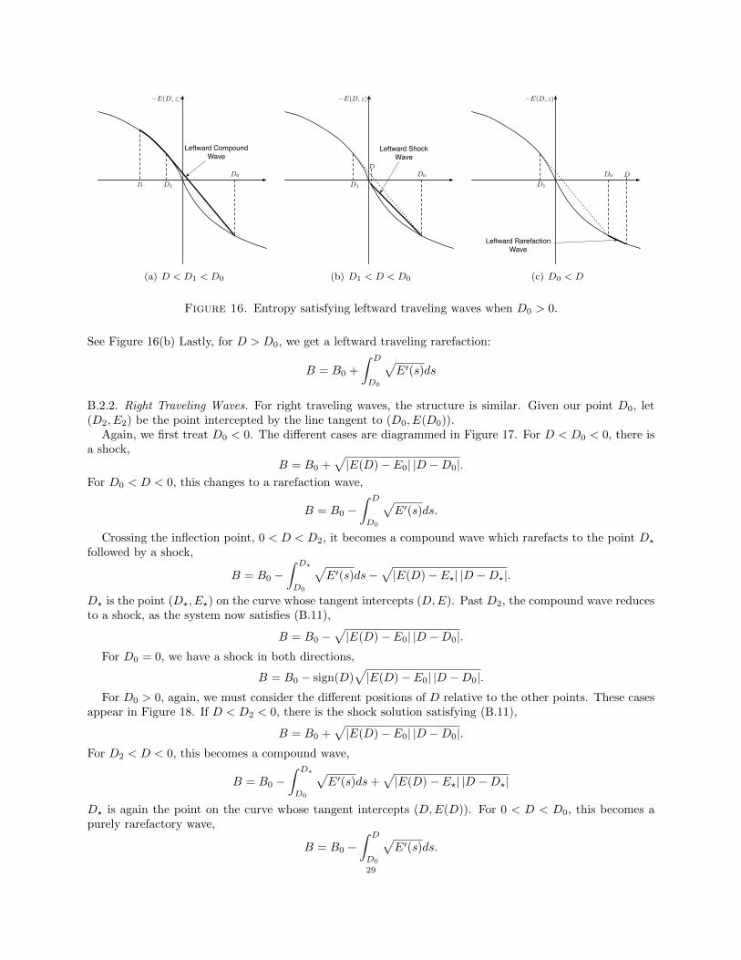
For D0 > 0, There are again several cases. For D < D1, we have the compound wave again, as in Figure16(a):
B = B0 −√|E(D1)− E0| |D1 −D0|+
∫ D
D1
√E′(s)ds
As D increases in value and D1 < D < D0, we have a shock solution
B = B0 −√|E(D)− E0| |D −D0|
28
D1
D0
−E(D, z)
Leftward Compound Wave
D
(a) D < D1 < D0
D1
D0
−E(D, z)
Leftward Shock Wave
D
(b) D1 < D < D0
D1
D0
−E(D, z)
Leftward Rarefaction Wave
D
(c) D0 < D
Figure 16. Entropy satisfying leftward traveling waves when D0 > 0.
See Figure 16(b) Lastly, for D > D0, we get a leftward traveling rarefaction:
B = B0 +
∫ D
D0
√E′(s)ds
B.2.2. Right Traveling Waves. For right traveling waves, the structure is similar. Given our point D0, let(D2, E2) be the point intercepted by the line tangent to (D0, E(D0)).
Again, we first treat D0 < 0. The different cases are diagrammed in Figure 17. For D < D0 < 0, there isa shock,
B = B0 +√|E(D)− E0| |D −D0|.
For D0 < D < 0, this changes to a rarefaction wave,
B = B0 −∫ D
D0
√E′(s)ds.
Crossing the inflection point, 0 < D < D2, it becomes a compound wave which rarefacts to the point D?
followed by a shock,
B = B0 −∫ D?
D0
√E′(s)ds−
√|E(D)− E?| |D −D?|.
D? is the point (D?, E?) on the curve whose tangent intercepts (D,E). Past D2, the compound wave reducesto a shock, as the system now satisfies (B.11),
B = B0 −√|E(D)− E0| |D −D0|.
For D0 = 0, we have a shock in both directions,
B = B0 − sign(D)√|E(D)− E0| |D −D0|.
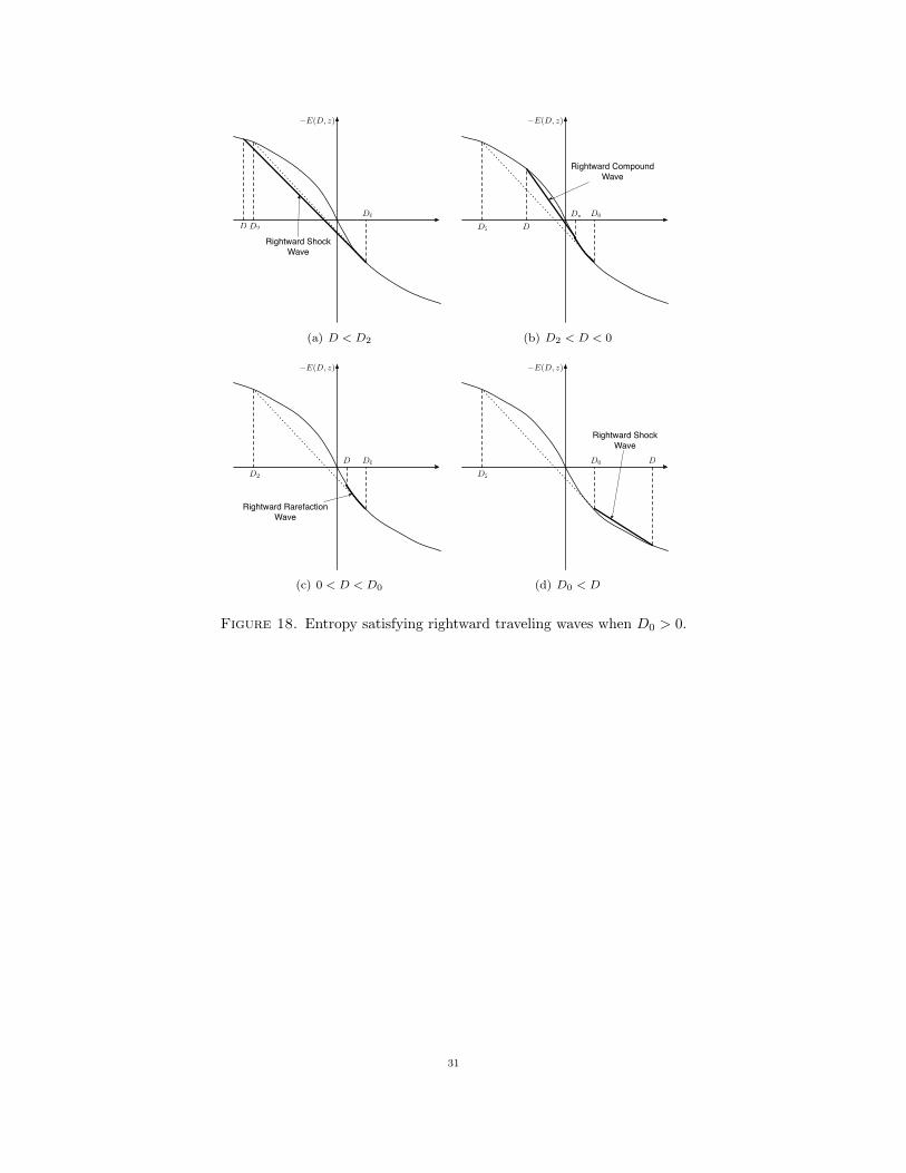
For D0 > 0, again, we must consider the different positions of D relative to the other points. These casesappear in Figure 18. If D < D2 < 0, there is the shock solution satisfying (B.11),
B = B0 +√|E(D)− E0| |D −D0|.
For D2 < D < 0, this becomes a compound wave,
B = B0 −∫ D?
D0
√E′(s)ds+
√|E(D)− E?| |D −D?|
D? is again the point on the curve whose tangent intercepts (D,E(D)). For 0 < D < D0, this becomes apurely rarefactory wave,
B = B0 −∫ D
D0
√E′(s)ds.
29

D0
D2
−E(D, z)
Rightward Shock Wave
D
(a) D < D0
D0
D2
−E(D, z)
Rightward Rarefaction Wave
D
(b) D0 < D < 0
D0
D2
−E(D, z)
Rightward Compound Wave
D
D�
(c) 0 < D < D2
D0
D2
−E(D, z)
Rightward Shock Wave
D
(d) D2 < D
Figure 17. Entropy satisfying rightward traveling waves when D0 < 0.
Finally, for D > D0, we again have a shock,
B = B0 −√|E(D)− E0| |D −D0|.
E-mail address: [email protected]
Mathematics Department, University of Toronto, Toronto, Ontario, Canada
E-mail address: [email protected]
Applied Mathematics Department, Columbia University, New York City, NY 10027, USA
30
D0
D2
−E(D, z)
Rightward Shock Wave
D
(a) D < D2
D0
D2
−E(D, z)
Rightward Compound Wave
D
D�
(b) D2 < D < 0
D0
D2
−E(D, z)
Rightward Rarefaction Wave
D
(c) 0 < D < D0
D0
D2
−E(D, z)
Rightward Shock Wave
D
(d) D0 < D
Figure 18. Entropy satisfying rightward traveling waves when D0 > 0.
31