Collateral Constraints and Macroeconomic Asymmetries∗

Luca Guerrieri†

Federal Reserve BoardMatteo Iacoviello‡

Federal Reserve Board

February 26, 2013

Abstract

A simple macroeconomic model with collateral constraints displays strong asymmetric re-

sponses to house price increases and declines. House price increases relax collateral constraints,

and the response of aggregate consumption, hours and output to a housing wealth shock is

positive but small. House price declines tighten collateral constraints, and the response of con-

sumption to a given change in housing values is negative and large. In experiments from the

model, we show how the response of consumption to shocks to housing wealth can be much

larger when house prices are low than when they are high. In line with the model, a simple

non-linear VAR estimated on U.S. national data shows that the response of consumption is less

sensitive to housing price increases than to declines. This finding is corroborated using regional

(state and MSA level) data. Our results imply that wealth effects computed in normal times

might severely underpredict the response of the economy to large house price declines, and that

public policies aimed at helping the housing market may be far more effective during protracted

housing downturns.

KEYWORDS: Housing, Collateral Constraints, Occasionally Binding Constraints.

JEL CODES: E32, E44, E47, R21, R31

∗The views expressed in this paper are those of the authors and do not necessarily reflect the views of theBoard of Governors of the Federal Reserve System. Replication codes that implement our solution technique forany DSGE model with occasionally binding constraints (irreversible capital, zero bound, occasionally binding bor-rowing constraints) using an add-on to Dynare are available upon request. Stedman Hood and Walker Ray per-formed superb research assistance on this project. Supplemental material is available at http://www2.bc.edu/matteo-iacoviello/research.htm.

†Luca Guerrieri, Office of Financial Stability, Federal Reserve Board, 20th and C St. NW, Washington, DC 20551.Email: luca.guerrieri@frb.gov

‡Matteo Iacoviello, Division of International Finance, Federal Reserve Board, 20th and C St. NW, Washington,DC 20551. Email: matteo.iacoviello@frb.gov

1

1 Introduction

Accounts of the recent financial crisis attribute a central role to the collapse in housing wealth

and to financial frictions in explaining the sharp contraction in consumption and overall economic

activity.1 Prior to the crisis, however, the increase in housing wealth associated with the steady

increase in house prices between 2001 and 2006 seems to have had much less influence in boosting

consumption. Taken together, these observations hard appear to reconcile with the notion that

the importance of housing collateral for macro aggregates is constant over the business cycle, and

suggest an asymmetry in the relationship between housing prices and economic activity. In this

paper, we argue that the sensitivity of macroeconomic aggregates to movements in housing wealth

can be large when housing wealth is low, and small when housing wealth is high. We develop this

argument in a quantitative general equilibrium model, and verify its predictions against U.S. data.

Our main story goes as follows. When house prices rise, households can borrow and spend

more, but the incentive and need to borrow more becomes proportionally smaller the larger is

the increase in house prices. As a consequence, the collateral channel from housing wealth to

consumption is positive but not large. Conversely, when house prices fall, collateral constraints are

tightened, and borrowing and expenditures co-move with house prices in a more dramatic fashion.

As a consequence, the macroeconomic consequences of declines in housing wealth are larger (and

more severe) than those of increases in housing wealth of equal magnitude but opposite sign. The

empirical analysis overwhelmingly supports the findings from the model that the fallout from a

decline in housing prices is much more severe than the boost to activity from an increase.

The model used in this paper is borrowed from Iacoviello and Neri (2010). It is an estimated

DSGE model that allows for numerous empirically-realistic nominal and real rigidities as in Chris-

tiano, Eichenbaum, and Evans (2005) and Smets and Wouters (2007). In addition, the model

encompasses a housing sector. On the supply side, a separate sector produces new homes using

capital, labor, and land. On the demand side, households consume housing services and can use

housing as a collateral for loans. In characterizing the properties of the model, we focus on a shock

to households preferences for housing. When house prices decline, household wealth is reduced,

collateral constraints become binding, and the effective share of credit-constrained households in-

creases. In contrast, house price increases relax households’ borrowing constraints. Iacoviello and

Neri (2010) solve this model using a first-order perturbation method. As a result, the importance

of credit-constrained agents remains constant and the effects of shocks that move house prices is

symmetric for increases and decreases. We deploy a non-linear solution technique that allows us to

capture asymmetric effects of shocks depending on whether the shocks push housing wealth up or

down. A simple moment-matching exercise shows that the data prefer a version of the model that

can generate a response of consumption and hours to house prices that is three times larger when

house prices fall than when they rise.

1 For instance, see Mian and Sufi (2010) and Hall (2011).

2

Figure 1 offers a first look at national house prices. It shows the evolution of U.S. house prices

over the period 1975-2012. To highlight their correlation properties, the top panel superimposes the

time series of U.S. house prices and of U.S. aggregation consumption expenditures. The correlation

coefficient is 0.55, a value substantial but not extreme. The bottom panel is a scatterplot of

changes in consumption and house prices. It highlights that most of the positive correlation seems

to be driven by periods when house prices are below average, both during the 1992-1993 period,

and during the 2007-2009 recession. When periods with house price decreases (the solid, magenta

line) are included, there is a strong positive correlation between consumption and house prices.

However, excluding periods with declines in house prices results in almost no correlation between

consumption and house prices.

We test the prediction of the model that house price increases and declines should have asym-

metric effects using both national and regional data. We proceed in two steps. First, we estimate

a VAR that includes U.S. consumption and house prices. Each equation in the VAR allows for

separate house price terms, depending on whether house prices increase or decrease. Estimates

of the VAR parameters based on data generated by the model imply a strong asymmetry in the

response of consumption to innovations in house prices, depending on whether the shock to house

prices is positive or negative. These population estimates are remarkably consistent with estimates

obtained using aggregate U.S. data.

In the second step, we use regional data. The task of isolating the asymmetric effect of changes

in house prices using national data only may be fraught with difficulty. Barring the Great Recession,

house price declines have been rare at the national level. In addition, knowing what would have

happened to economic activity had house prices not changed raises challenging identification issues.

Accordingly, we use panel and cross-sectional regressions at the regional level. Regional data exhibit

greater variation in house prices. Moreover, at the regional level, we can use instruments that other

studies have found useful in isolating exogenous changes in house prices. When we do so, we verify

that the asymmetries uncovered using national aggregate data are even more pronounced when we

use regional data.2

Our analysis builds on an expanding empirical literature that has linked changes in measures

of economic activity, such as consumption and employment, to changes in house prices. Recent

contributions include Case, Quigley, and Shiller (2005), Campbell and Cocco (2007), Mian and Sufi

(2011), Midrigan and Philippon (2011), Mian, Rao, and Sufi (2012) and Abdallah and Lastrapes

(2012). The emerging consensus from this literature points towards an important role for housing

as collateral for household credit in influencing both consumption and employment. However, such

literature has not recognized that such a channel implies asymmetric relationships for house price

2 We are fully aware of the notion that housing prices are endogenous both in theory and in the data. Our modelingstrategy attributes most of the variation in house prices to shocks to housing preferences (as in recent work by Liu,Wang, and Zha (2011) and Iacoviello and Neri (2010). Part of our empirical analysis looks for instruments for houseprice changes in a way to isolate housing preference shocks from other shocks that are more likely to jointly moveboth housing and other endogenous variables, as done by Mian and Sufi (2011).

3

increases and declines with other measures of aggregate activity. Furthermore, our uncovering of

statistically significant differences for house price increases and declines, as theory predicts, provides

more cogent support for the hypothesis that the housing collateral channel has played an important

role in linking house price fluctuations to other key measures of economic activity. In addition, an

important contribution of this paper is that we analyze this asymmetry not only empirically, but

also theoretically in the context of a quantitative equilibrium model.3

To the best of our knowledge, Case, Quigley, and Shiller (2005) and Case, Quigley, and Shiller

(2011) first highlighted the possibility, using U.S. state-level data, that house prices could have

asymmetric effects on consumption. Their 2011 paper, in particular, finds in many specifications

that declines in housing market wealth have had negative and somewhat larger effects upon con-

sumption than previous increases. Our analysis extends their work by considering a larger set of

variables and regional detail, and by tying the results to a full-blown equilibrium model.

The rest of the paper proceeds as follows: Section 2 presents a simple intuition for why collateral

constraints imply an asymmetry in the relationship between house prices and consumption using a

partial equilibrium model. Section 3 considers an empirically-validated general equilibrium model.

Section 4 highlights properties of the general equilibrium model and matches them against an

asymmetric VAR estimated on aggregate U.S. data. Section 5 presents additional evidence on

asymmetries in the relationship between house prices and other measures of economic activity

based on state and MSA-level data. Section 6 considers a policy experiment. Section 7 concludes.

2 Collateral Constraints and Asymmetries: A Basic Model

To fix ideas regarding the fundamental asymmetry introduced by collateral constraints, it is useful to

work through a simple model and analyze its implications for the size of the response of consumption

to changes in housing prices. Throughout this section, we sidestep obvious general equilibrium

considerations and assume that the price of housing is exogenous: we relax all these assumptions

in the DSGE model of the next section. Consider the problem of a household that has to choose

profiles for goods consumption ct, housing ht, and borrowing bt. The utility of the household is

given by

U = E0

∞∑t=0

βt (log ct + j log ht)

3 The idea that borrowing constraints may introduce asymmetric responses of consumption to shocks is a well-known result in macroeconomics. For instance, Jappelli and Pistaferri (2010) observe that if households are creditconstrained, they will cut consumption strongly when hit by a negative transitory shock but will not react much toa positive one.

4

where E0 is the conditional expectation operator. The budget and borrowing constraints are given

by:

ct + qtht = y + bt −Rbt−1 + qt (1− δh)ht−1; (1)

bt ≤ mqtht, (2)

where R denotes the gross one-period interest rate, and β is assumed to satisfy the restriction that

βR < 1, so that in a steady state without shocks the borrowing constraint is binding and leverage

(the ratio of debt to housing wealth) is at its upper bound given by m. The price of housing, qt, is

assumed to follow an AR(1) stochastic process, and income y is exogenously fixed and normalized

to one. Housing, which depreciates at rate δh, is used as collateral for borrowing, and qtht is the

value of collateral. The parameter m denotes the maximum loan-to-value ratio. Letting µt be the

Lagrange multiplier on the borrowing constraint, the consumption Euler equation is:

1

ct= βREt

(1

ct+1

)+ µt. (3)

In a steady state, µ > 0, and c = y − ((R− 1)m− δh) qh. Solving this equation forward and

log-linearizing around the steady state, one obtains the following expression for consumption in

percent deviation from steady state, ct:

ct = −1− βR

µEt

(µt − µ+ βR

(µt+1 − µ

)+ β2R2

(µt+2 − µ

)+ ...

). (4)

Expressing the Euler equation as above shows that consumption depends negatively on current

and future expected borrowing constraints. As shown by equation 2, increases in qt will loosen the

borrowing constraint. So long as they keep µt positive, increases and decreases in qt will have roughly

symmetric effects on ct. However, large enough increases in qt imply a fundamental asymmetry.

The multiplier µt cannot fall below zero. Consequently, large increases in qt can bring µt to its

lower bound and will have proportionally smaller effects on ct than decreases in qt. Intuitively, an

impatient borrower prefers a consumption profile that is declining over time. A large temporary

increase in house prices will enable such a profile (high c today, low c tomorrow) without borrowing

all the way up to the limit.

More formally, the household’s state at time t is its housing ht−1, debt bt−1 and the current

realization of the house price qt, and the optimal decision are given by the consumption choice

c (q, h, b) , the housing choice h′ (q, h, b) and the debt choice b′ (q, h, b) that maximize expected

utility subject to 1 and 2, given the house price process. Figure 2 illustrates the optimal leverage

and the consumption function obtained from the model above given the parameter values calibrated

and estimated in the next section.4 As the figure illustrates, large house price realizations move

4 Figure 2 shows the policy functions obtained solving the partial equilibrium model described in this sectionusing standard global methods. For the general equilibrium model described below in Section 3, we approximate the

5

the household in a region where the borrowing constraint is not binding. When the constraint is

not binding, consumption becomes less sensitive to changes in house prices. Instead, when the

household is borrowing constrained, so that leverage is at its maximum level – something that

happens when house prices are low and initial stock debt is high – the sensitivity of consumption

to changes in house prices becomes large.

3 The Full Model

To quantify the importance of the asymmetric relationship between house prices and consumption,

we now embed the basic ideas of Section 2 in an empirically validated general equilibrium model.

The model is borrowed from Iacoviello and Neri (2010). It builds on Christiano, Eichenbaum,

and Evans (2005) and Smets and Wouters (2007) by allowing for two sectors, a housing sector and

non-housing a sector, as well as financial frictions and borrowing collateralized by housing following

Iacoviello (2005).

On the supply side, firms in the housing sector produce new homes using capital, labor and

land. Firms in the non-housing sector produce intermediate consumption and investment goods

using capital and labor. The non-housing sector features nominal price rigidities. Both sectors

have nominal wage rigidities and real rigidities in the form of imperfect labor mobility, capital

adjustment costs and variable capital utilization.

On the household side, there is a continuum of agents in each of two groups that display different

discount factors. Households in the group with the higher discount factor are dubbed “patient,” the

other “impatient.” Patient households accumulate housing and own the productive capital of they

economy. They make consumption and investment decisions and supply labor to firms and funds

to both firms and impatient households. Impatient households work, consume, and accumulate

housing. Their higher impatience pushes them to borrow. In the non-stochastic steady state, their

housing collateral constraint is binding.

Below, we sketch the key features of the model. Appendix B provides the list of all necessary

conditions for an equilibrium.

solution using the methods described on page 10 (for the simple model of this section, Appendix A compares theproperties of the solution methods). The parameter values match those of Table 1 and are: β = 0.988, j = 0.12,m = 0.925, R = 1.01, δ = 0.01. The resulting steady-state housing wealth to quarterly income ratio is 6.1, close tothe housing wealth to income ratio for impatient households in the steady state of the extended model. Finally, thehouse price process is described by an AR(1) process of the form

log qt = ρq log qt−1 + εq

with autocorrelation given by ρq = 0.96 and standard deviation equal of εq equal to 0.0169, in order to match astandard deviation of the quarterly growth rate of house prices equal to 1.71 percent, as in the data.

6

3.1 Households

Within each group of patient and impatient households, a representative household maximizes:

E0∑∞

t=0 (βGC)t zt

(Γc ln (ct − εct−1) + jt lnht −

τ t1 + η

(n1+ξc,t + n1+ξ

h,t

) 1+η1+ξ

);

E0∑∞

t=0

(β′GC

)tzt

(Γ′c ln(c′t − ε′c′t−1

)+ jt lnh

′t −

τ t1 + η′

((n′c,t

)1+ξ′+(n′h,t

)1+ξ′) 1+η′

1+ξ′

). (5)

Variables accompanied by the prime symbol refer to patient households. c, h, nc, nh are con-

sumption, housing, hours in the consumption sector and hours in the housing sector. The discount

factors are β and β′. By definition, β′ < β. The terms zt , jt, and τ t capture shocks to intertemporal

preferences, labor supply, and housing preferences, respectively. The shocks follow:

ln zt = ρz ln zt−1 + uz,t, ln jt =(1− ρj

)ln j + ρj ln jt−1 + uj,t, ln τ t = ρτ ln τ t−1 + uτ,t, (6)

where uz,t, uj,t, uτ,t and are i.i.d. processes with variances σ2z, σ

2j , and σ2

τ . Above, ε measures

habits in consumption and GC is the growth rate of consumption along the balanced growth path.

The scaling factors Γc = (GC − ε) / (GC − βεGC) and Γ′c = (GC − ε′) /

(GC − β′ε′GC

)ensure that

the marginal utilities of consumption are 1/c and 1/c′ in the non-stochastic steady state.

Patient households accumulate capital and houses and make loans to impatient households.

They rent capital to firms, choose the capital utilization rate; in addition, there is joint production

of consumption and business investment goods. Patient households maximize their utility subject

to:

ct +kc,tAk,t

+ kh,t + kb,t + qtht + pl,tlt − bt =wc,tnc,t

Xwc,t+

wh,tnh,t

Xwh,t

+

(Rc,tzc,t +

1− δkcAk,t

)kc,t−1 + (Rh,tzh,t + 1− δkh) kh,t−1 + pb,tkb,t −

Rt−1bt−1

πt

+(pl,t +Rl,t) lt−1 + qt (1− δh)ht−1 +Divt − ϕt −a (zc,t) kc,t−1

Ak,t− a (zh,t) kh,t−1. (7)

Patient agents choose consumption ct, capital in the consumption sector kc,t, capital kh,t and

intermediate inputs kb,t (priced at pb,t) in the housing sector, housing ht (priced at qt), land lt (priced

at pl,t), hours nc,t and nh,t, capital utilization rates zc,t and zh,t, and borrowing bt (loans if bt is

negative) to maximize utility subject to (8). The term Ak,t captures investment-specific technology

shocks, thus representing the marginal cost (in terms of consumption) of producing capital used in

the non-housing sector. Loans are set in nominal terms and yield a riskless nominal return of Rt.

Real wages are denoted by wc,t and wh,t, real rental rates by Rc,t and Rh,t, depreciation rates by δkc

and δkh. The terms Xwc,t and Xwh,t denote the markup (due to monopolistic competition in the

labor market) between the wage paid by the wholesale firm and the wage paid to the households,

7

which accrues to the labor unions (we discuss below the details of nominal rigidities in the labor

market). Finally, πt = Pt/Pt−1 is the money inflation rate in the consumption sector, Divt are

lump-sum profits from final good firms and from labor unions, ϕt denotes convex adjustment costs

for capital, z is the capital utilization rate that transforms physical capital k into effective capital

zk and a (·) is the convex cost of setting the capital utilization rate to z.

Impatient households do not accumulate capital and do not own finished good firms or land

(their dividends come only from labor unions). In addition, their maximum borrowing b′t is given

by the expected present value of their home times the loan-to-value (LTV) ratio mt:

c′t + qth′t − b′t = w′

c,tn′c,t/X

′wc,t + w′

h,tn′h,t/X

′wh,t + qt (1− δh)h

′t−1 −Rt−1b

′t−1/πt +Div′t; (8)

b′t ≤ mtEt

(qt+1h

′tπt+1

Rt

). (9)

Departing slightly from Iacoviello and Neri (2010), we also allow for shocks to the LTV ratio

governed by an auto-regressive process.

3.2 Firms

To allow for nominal price rigidities, the models differentiates between competitive flexible price/wholesale

firms that produce wholesale consumption goods and housing using two distinct technologies, and

a final good firm (described below) that operates in the consumption sector under monopolistic

competition. Wholesale firms hire labor and capital services and purchase intermediate goods to

produce wholesale goods Yt and new houses IHt. They solve:

maxYtXt

+ qtIHt −

( ∑i=c,h

wi,tni,t +∑

i=c,h

w′i,tn

′i,t +

∑i=c,h

Ri,tzi,tki,t−1 +Rl,tlt−1 + pb,tkb,t

).

Above, Xt is the markup of final goods over wholesale goods. The production technologies are:

Yt =(Ac,t

(nαc,tn

′1−αc,t

))1−µc (zc,tkc,t−1)µc ; (10)

IHt =(Ah,t

(nαh,tn

′1−αh,t

))1−µh−µb−µl(zh,tkh,t−1)

µh kµbb,tl

µlt−1. (11)

In (11), the non-housing sector produces output with labor and capital. In (12), new homes are

produced with labor, capital, land and the intermediate input kb. The terms Ac,t and Ah,t measure

productivity in the non-housing and housing sector, respectively.

8

3.3 Nominal Rigidities and Monetary Policy

There are Calvo-style price rigidities in the non-housing consumption sector and wage rigidities in

both sectors. The resulting consumption-sector Phillips curve is:

lnπt − ιπ lnπt−1 = βGC (Et lnπt+1 − ιπ lnπt)− επ ln (Xt/X) + up,t (12)

where επ = (1−θπ)(1−βGCθπ)θπ

. Above, i.i.d. cost shocks up,t are allowed to affect inflation indepen-

dently from changes in the markup. These shocks have zero mean and variance σ2p.

Wage setting is modelled in an analogous way. Patient and impatient households supply homo-

geneous labor services to unions. The unions differentiate labor services as in Smets and Wouters

(2007), set wages subject to a Calvo scheme and offer labor services to wholesale labor packers

who reassemble these services into the homogeneous labor composites nc, nh, n′c, n

′h. Wholesale

firms hire labor from these packers. Under Calvo pricing with partial indexation to past inflation,

the pricing rules set by the union imply four wage Phillips curves that are isomorphic to the price

Phillips curve.

Monetary policy follows an interest rate rule that responds gradually to inflation and GDP

growth:

Rt = RrRt−1π

(1−rR)rπt

(GDPt

GCGDPt−1

)(1−rR)rY

rr1−rRuR,t

st. (13)

GDP is the weighted average of output in the two sectors with nominal share weights fixed at

their values in the non-stochastic steady state. The term rr is the steady-state real interest rate;

uR,t is an i.i.d. monetary shock with variance σ2R ; st is a stochastic process with high persistence

capturing long-lasting deviations of inflation from its steady-state level, due e.g. to shifts in the

central bank’s inflation target. That is, ln st = ρs ln st−1 + us,t, us,t ∼ N (0, σs) , where ρs > 0.

3.4 Market Clearing Conditions

The goods market produces consumption, business investment and intermediate inputs. The hous-

ing market produces new homes IHt. The equilibrium conditions are:

Ct + IKc,t/Ak,t + IKh,t + kb,t = Yt − ϕt; (14)

Ht − (1− δh)Ht−1 = IHt, (15)

together with the loan market equilibrium condition. Above, Ct = ct+c′t is aggregate consumption,

Ht = ht + h′t is the aggregate stock of housing, and IKc,t = kc,t − (1− δkc) kc,t−1 and IKh,t =

kh,t − (1− δkh) kh,t−1 are the two components of business investment. Total land is fixed and

normalized to one.

9

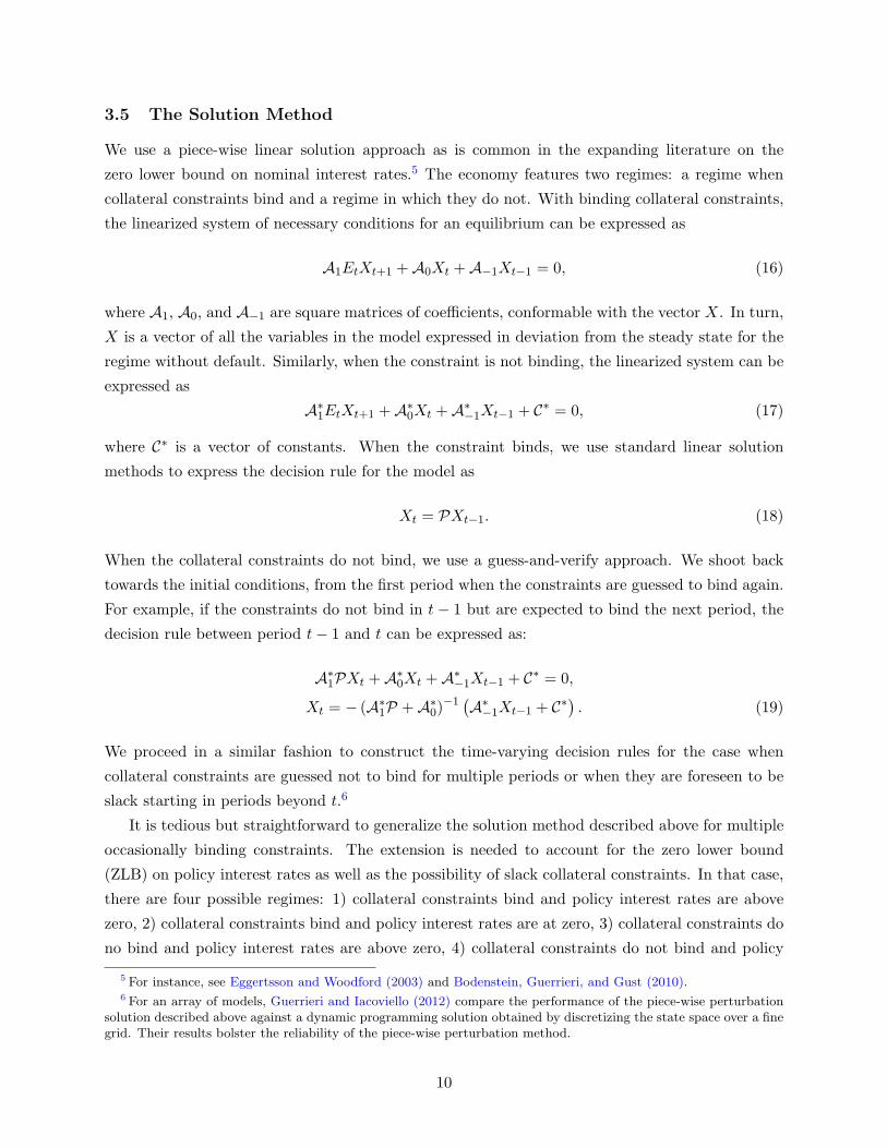
3.5 The Solution Method

We use a piece-wise linear solution approach as is common in the expanding literature on the

zero lower bound on nominal interest rates.5 The economy features two regimes: a regime when

collateral constraints bind and a regime in which they do not. With binding collateral constraints,

the linearized system of necessary conditions for an equilibrium can be expressed as

A1EtXt+1 +A0Xt +A−1Xt−1 = 0, (16)

where A1, A0, and A−1 are square matrices of coefficients, conformable with the vector X. In turn,

X is a vector of all the variables in the model expressed in deviation from the steady state for the

regime without default. Similarly, when the constraint is not binding, the linearized system can be

expressed as

A∗1EtXt+1 +A∗

0Xt +A∗−1Xt−1 + C∗ = 0, (17)

where C∗ is a vector of constants. When the constraint binds, we use standard linear solution

methods to express the decision rule for the model as

Xt = PXt−1. (18)

When the collateral constraints do not bind, we use a guess-and-verify approach. We shoot back

towards the initial conditions, from the first period when the constraints are guessed to bind again.

For example, if the constraints do not bind in t− 1 but are expected to bind the next period, the

decision rule between period t− 1 and t can be expressed as:

A∗1PXt +A∗

0Xt +A∗−1Xt−1 + C∗ = 0,

Xt = − (A∗1P +A∗

0)−1 (A∗

−1Xt−1 + C∗) . (19)

We proceed in a similar fashion to construct the time-varying decision rules for the case when

collateral constraints are guessed not to bind for multiple periods or when they are foreseen to be

slack starting in periods beyond t.6

It is tedious but straightforward to generalize the solution method described above for multiple

occasionally binding constraints. The extension is needed to account for the zero lower bound

(ZLB) on policy interest rates as well as the possibility of slack collateral constraints. In that case,

there are four possible regimes: 1) collateral constraints bind and policy interest rates are above

zero, 2) collateral constraints bind and policy interest rates are at zero, 3) collateral constraints do

no bind and policy interest rates are above zero, 4) collateral constraints do not bind and policy

5 For instance, see Eggertsson and Woodford (2003) and Bodenstein, Guerrieri, and Gust (2010).6 For an array of models, Guerrieri and Iacoviello (2012) compare the performance of the piece-wise perturbation

solution described above against a dynamic programming solution obtained by discretizing the state space over a finegrid. Their results bolster the reliability of the piece-wise perturbation method.

10

interest rates are at zero. Apart from the proliferation of cases, the main ideas outlined above still

apply.

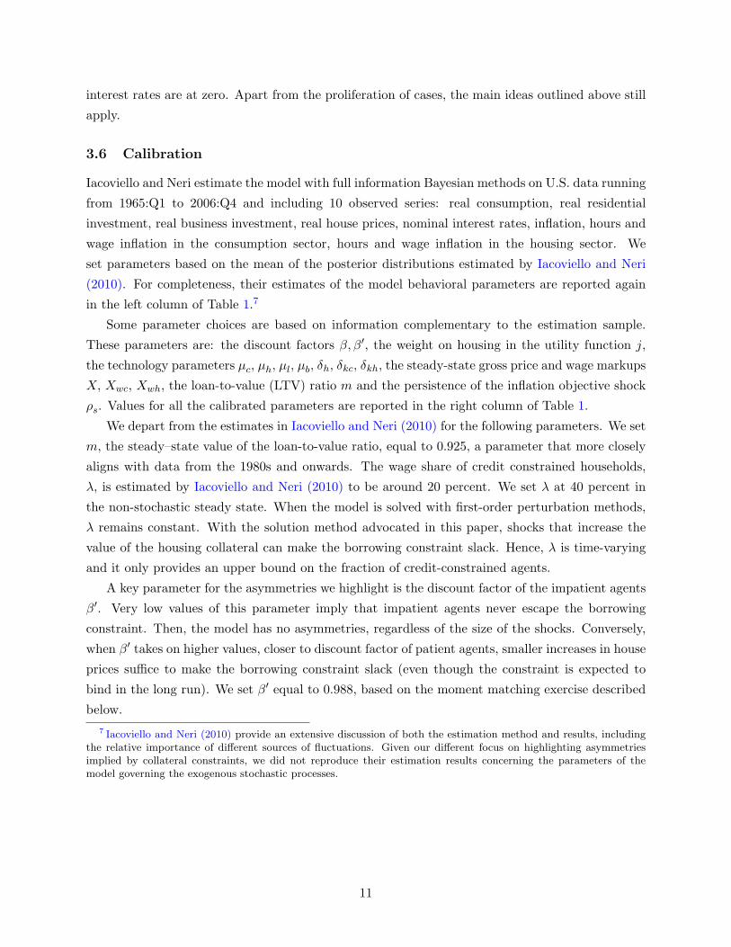
3.6 Calibration

Iacoviello and Neri estimate the model with full information Bayesian methods on U.S. data running

from 1965:Q1 to 2006:Q4 and including 10 observed series: real consumption, real residential

investment, real business investment, real house prices, nominal interest rates, inflation, hours and

wage inflation in the consumption sector, hours and wage inflation in the housing sector. We

set parameters based on the mean of the posterior distributions estimated by Iacoviello and Neri

(2010). For completeness, their estimates of the model behavioral parameters are reported again

in the left column of Table 1.7

Some parameter choices are based on information complementary to the estimation sample.

These parameters are: the discount factors β, β′, the weight on housing in the utility function j,

the technology parameters µc, µh, µl, µb, δh, δkc, δkh, the steady-state gross price and wage markups

X, Xwc, Xwh, the loan-to-value (LTV) ratio m and the persistence of the inflation objective shock

ρs. Values for all the calibrated parameters are reported in the right column of Table 1.

We depart from the estimates in Iacoviello and Neri (2010) for the following parameters. We set

m, the steady–state value of the loan-to-value ratio, equal to 0.925, a parameter that more closely

aligns with data from the 1980s and onwards. The wage share of credit constrained households,

λ, is estimated by Iacoviello and Neri (2010) to be around 20 percent. We set λ at 40 percent in

the non-stochastic steady state. When the model is solved with first-order perturbation methods,

λ remains constant. With the solution method advocated in this paper, shocks that increase the

value of the housing collateral can make the borrowing constraint slack. Hence, λ is time-varying

and it only provides an upper bound on the fraction of credit-constrained agents.

A key parameter for the asymmetries we highlight is the discount factor of the impatient agents

β′. Very low values of this parameter imply that impatient agents never escape the borrowing

constraint. Then, the model has no asymmetries, regardless of the size of the shocks. Conversely,

when β′ takes on higher values, closer to discount factor of patient agents, smaller increases in house

prices suffice to make the borrowing constraint slack (even though the constraint is expected to

bind in the long run). We set β′ equal to 0.988, based on the moment matching exercise described

below.

7 Iacoviello and Neri (2010) provide an extensive discussion of both the estimation method and results, includingthe relative importance of different sources of fluctuations. Given our different focus on highlighting asymmetriesimplied by collateral constraints, we did not reproduce their estimation results concerning the parameters of themodel governing the exogenous stochastic processes.

11

4 Results of the Full Model

First, we complete the calibration of the model through a model matching exercise. Second, we

use a simple non-linear VAR to investigate the asymmetric relationship between house prices and

consumption. The VAR implied by population moments from our model captures asymmetric

responses of consumption to house price increases and declines. The VAR estimated on the observed

data sample is consistent with its model counterpart.

4.1 A Moment Matching Exercise

We use the model to generate data conditional on two sources of stochastic variation: an AR(1)

process that governs the loan-to-value ratio, mt; and a shock to housing preferences jt. We single

these two shocks out because several studies have suggested that movements in housing demand

and credit market shocks may play an important role in driving housing prices and aggregate

consumption. Another advantage of these two shocks is that the housing demand shock primarily

drives housing prices and, to the extent that there are strong collateral channels, affects consumption

as well. The shock to the loan-to-value ratio affects consumption relatively more, since it influences

the short-term resources that borrowers use to finance consumption. We choose the standard

deviations of the two shocks and the discount factor of the impatient agents in order to optimize the

model’s ability to account for the volatility of consumption and house prices and their correlation.

Importantly, we do not impose any requirements on the model’s ability to fit higher moments in

the data, such as asymmetries in the responses to shocks. The metric used in our optimization

procedure is L(ss) , where ss is the vector including estimates of σj , σm, β′ and L(ss) is given by

L (ss) = (mm− f (ss)) V −1 (mm− f (ss))′ .

Here, mm is a 3× 1 vector that includes the sample standard deviation of quarterly consumption

growth and quarterly real house price growth, as well as their correlation. The 3 × 3 matrix V is

the identity matrix. Finally, f (ss) is a 3×1 vector with moments analogous to the ones in mm but

implied by the model in population (with all other parameters set as described in the calibration

section above). The parameter values that minimize L(ss) are σj = 0.0825 , σm = 0.0205, and

β′ = 0.988.

As a cross check, the standard deviations of quarterly consumption growth and house price

growth implied by the model in population are 0.66 and 1.71 percent, very close to their observed

sample counterparts of 0.63 and 1.77 percent. The correlation of consumption growth and house

price growth implied by the model in population is 0.42, also close to its observed sample counterpart

of 0.39.

12

4.2 A Nonlinear VAR

With the estimates above, we use model-generated data on consumption and housing prices to fit a

two-variable nonlinear VAR. Each equation in the VAR regresses linearly detrended consumption

and house prices on: a constant, the linearly detrended consumption, and distinct terms for positive

and negative lagged deviations of housing prices from a linear trend.8 Innovation to each equation

are orthogonalized using a Cholesky scheme: we treat model and data symmetrically, by imposing

an ordering scheme such that a “house price shock” affects contemporaneously both house prices

and consumption.

Figure 3 shows population estimates from the model (the thin lines) against estimates for U.S.

data running from 1975 to 2011 (the thick lines) and 95% bootstrap confidence bands. The top

panels focus on innovations to house prices that yield about a 2 standard deviation increase in

house prices. The bottom panels show responses to an innovation that brings about a 2 standard

deviation decline in house prices. Strikingly, model and data appear in substantial agreement: the

response of consumption to a large house price decline is twice as large than that to a large house

price increase of equal magnitude, in the model as in the data. Furthermore, for the estimates based

on observed data, we compute confidence intervals for the difference between the peak response of

the absolute value of consumption to the positive and negative innovations. We confirm that this

difference is statistically different from zero at standard significance levels. Accordingly, we fail to

reject the null hypothesis of asymmetric responses.

4.3 Responses to Positive and Negative Shocks

To illustrate the fundamental source of the asymmetry in the model, Figure 4 considers the effects

of a shock to housing preferences, the process jt in Equation (5), which we interpret as a shock

to housing demand. Between periods 1 and 10, a series of innovations to jt are set to bring

about a decline in house prices of 30 percent.9 Thereafter, the shock follows its autoregressive

process. In this case, the decrease in house prices reduces the collateral capacity of constrained

households. Accordingly those households can borrow less and are forced to curtail their non-

housing consumption even further in order to comply with the borrowing constraint. On balance,

the decline in aggregate consumption is close to 5 percent. The new-Keynesian channels in the

model imply that the large decline in aggregate consumption translate into a large decline in the

firms’ demand for labor. In equilibrium, the drop in hours worked comes close to reaching 6 percent

below the balanced growth path.

8 In other words, the right-hand side variables in the VAR are (aside from the constant term) the lag of ct,max (qt, 0) , and min(qt, 0), where ct and qt denote the log deviations of consumption and house prices from theirrespective linear trends.

9 Iacoviello and Neri (2010) find that house preference shocks are one of the key determinants of house pricemovements at business cycle frequencies. Similarly, Liu, Wang, and Zha (2011) highlight that a shift in housingdemand in a credit-constrained economy can lead to large fluctuations in land prices, an produce a broader impacton hours worked and output.

13

Unforseen to the agents in the model, in period 51 a series of innovations for the shock to housing

preferences brings about a 30 percent increase in house prices over the next 10 quarters. Recalling

the partial equilibrium model described in Section 2, an increase in house prices can relax borrowing

constraints. After a short two quarters, the borrowing constraint for the representative impatient

household becomes slack. The Lagrange multiplier in the households’ utility maximization problem

bottoms out at zero. In period 61, the shock to housing preferences starts following its autoregressive

process and house prices begin to decline. The borrowing constraint remains slack for another couple

of quarters, but even as house prices are well above their balanced growth path, the borrowing

constraint starts binding again (and its Lagrange multiplier takes on positive values).

When the constraint becomes slack, the borrowing constraint channel remains operative only

in expectation. Thus, impatient households discount that channel more heavily the longer the

constraint is expected to remain slack. As a consequence, the response of consumption to the large

house price increases considered in the figure is not as dramatic as the reaction to house price

declines of an equal magnitude. At peak the increase in consumption and hours worked is about 2

percent, respectively 1/2 and 1/3 of the response to the house price declines.

Figure 5 plots the peak response of consumption to a house demand shock as a function of

the change in house prices induced by the same shock. The figure also shows the relationship

between the peak elasticity of consumption to housing wealth as a function of the peak impact to

housing wealth. Prosaically, the former is defined as the ratio of the peak response of aggregate

consumption to the peak response of house wealth, the latter as the peak response of the value of the

housing stock. In our model, if borrowing constraints were always binding, this elasticity would be

constant, regardless of the change in house prices. However, because large increases in house prices

can make the borrowing constraint slack, they affect consumption less and less. Mechanically, the

peak impact on consumption of a housing demand shock continues to decline because our solution

algorithm attributes a longer duration to the regime with slack borrowing constraints when the

house price increases become larger.

After observing a long string of house price increases, an econometrician running a linear regres-

sion would be tempted to conclude that the spillovers from house prices to aggregate consumption

are modest. However, the same econometrician would produce quite different estimates after a

string of house price declines.

4.4 Sensitivity Analysis

Figure 7 considers again the peak impact of consumption relative to the peak impact on house prices

of a housing demand shock. For ease of comparison, the blue solid line reproduces the benchmark

results shown in Figure 5. In addition, Figure 7 considers two alternative calibrations. The dashed

black line, labelled “High Impatience” focuses on a lower discount factor for impatient agents,

setting β′ equal to 0.98. Focusing on the bottom panel of the figure, with greater impatience,

larger increases in house prices are required to relax the borrowing constraint. Accordingly, the

14

peak elasticity of consumption to housing wealth remains constant for larger increases in housing

wealth than under the benchmark calibration. Moreover, even when the borrowing constraint is

eventually relaxed by larger underlying housing demand shocks, the constraint is expected to stay

slack for a shorter period than under the benchmark. These differences are also reflected in the top

panel. The flattening out of the response of consumption to increases in housing wealth becomes

less pronounced.

The dot-dashed, red lines in Figure 7 show results for a lower value of the LTV ratio, with

m equal to 0.75. When increases in housing wealth make the borrowing constraint slack, there

are little differences between the benchmark and the results under this alternative calibration. If

anything, for large increases in house prices, the response of consumption is stronger, since the

borrowing constraint is likely to be less slack, and the collateral effect stronger, for low values of

the LTV ratio. However, when housing wealth declines, the collateral effect is smaller, and the

decrease in borrowing is less pronounced. Accordingly, lower values for m also imply al flattening

of the response of consumption to increases in housing wealth and a compression of the asymmetry

that we have highlighted so far.

Moving in the opposite direction, Figure 6 considers a mechanism that can enhance the asym-

metric response of consumption to housing demand shocks. In addition to the baseline model

already considered in Figure 5, it considers a variant of the model, labelled “ZLB”, that allows for

another occasionally binding constraint, namely the zero lower bound on the policy interest rate.

In that case, the Monetary policy rule becomes:

Rt = max

[1, RrR

t−1π(1−rR)rπt

(GDPt

GCGDPt−1

)(1−rR)rY

rr1−rRuR,t

st

]. (20)

In the ZLB case, sufficiently large price declines can bring the gross policy rate Rt to 1 (equivalently,

the net policy rate hits 0). With mechanisms familiar from the literature on the effects of aggregate

demand shocks in a liquidity trap,10 the spillover effects of contractionary housing demand shocks

onto aggregate consumption become amplified. At the zero lower bound with constant nominal

rates, declines in inflation can bring up real interest rates and deepen the contractionary effects of

the shock. We pick up this theme again below when discussing our estimates from panel regressions

on regional data.

5 Regional Evidence on Asymmetries

The results of our theoretical model and the evidence from the vector autoregressions at the national

level motivate additional empirical analysis that we conduct using a panel of data from U.S. states

and Metropolitan Statistical Areas (MSA). The obvious advantage of these data is that variation

in housing prices and economic activity is greater at the regional than at the aggregate level, as

10 For instance, see Christiano, Eichenbaum, and Rebelo (2011).

15

documented for instance by Del Negro and Otrok (2007), who find a large degree of heterogeneity

across states in regard to relative importance of the national factors. The use of regional data also

allays the concern that little can be learned using national data, given the rarity of declines in

house prices at the national level.

In order to set the stage, Figure 8 shows changes in house prices and changes in employment

in the service sector, auto sales, electricity consumption, and mortgage originations in 2005 and

2008 for all the 50 U.S. states and the District of Columbia. For each state there are two dots in

each panel: the green dot (concentrated in the north–east region of the graph) shows the lagged

percent change in house prices and the percent change in the indicator of economic activity in 2005,

at the height of the housing boom.11 The red dot represents analogous observations for the 2008

period, in the midst of the housing crash. Fitting a piecewise linear regression to these data yields

a correlation between house prices and activity that is smaller when house prices are high. This

evidence on asymmetry is bolstered by the large cross-sectional variation in house prices across

states over the period in question.

5.1 State-Level Evidence

We use annual data from 1990 to 2011 from the 50 U.S. states and the District of Columbia on

house prices and measures of economic activity. We choose measures of economic activity to match

our model counterparts for consumption, employment and credit.

Our main specification takes the following form:

∆ log yi,t = αi + γt + βPOSIi,t∆log hpi,t−1 + βNEG (1− Ii,t)∆ log hpi,t−1 + δXi,t−1 + εi,t

where yi,t is an index of economic activity and hpi,t is the inflation-adjusted house price index in

state i in period t; αi and γt represent state and year fixed effects; and Xi,t is a vector of additional

controls. We interact changes in house prices with a state-specific indicator variable Ii,t that takesvalue 1 when house prices are high, and value 0 when house prices are low. We classify house prices

as high in a particular state when house prices are above a state-specific linear trend estimated for

the 1975-2010 period. Using this approach, the fraction of states with high house prices is about

20 percent in the 1990s, rises gradually to peak at 100 percent in 2005 and 2006, and drops to 27

percent in 2010. Our results were similar using a different definition of Ii,t that takes value 1 when

real house price inflation is positive. In our baseline specification, we use one-year lags of house

prices and other controls to control for obvious endogeneity concerns. Our results were also little

changed when instrumenting current or lagged house prices with one or more lags.

Tables 2 to 5 present our estimates when the indicators of economic activity yi,t are employment

in the service sector, automobile sales, electricity usage and mortgage originations respectively.12

11 An analogous relationship is more tenuous for house prices and employment in the manufacturing goods sector.Most goods are traded and are less sensitive to local house prices than services.

12 In the sample period we analyze, the first principal component for annual house price growth accounts for 64

16

Table 2 presents the results for our preferred measure of regional economic activity, namely

employment in the non-tradeable service sector. We choose this measure (rather than, say, total

employment) since U.S. states (and MSAs) heavily trade with each other, so that employment in

sectors that mainly produce for the local economy better isolates the local effects of movements

in local house prices.13 The first two columns do not control for time effects. They show that the

asymmetry is strong and economically important, and that house prices matter, at statistically

conventional levels, both when high and when low. After controlling for time effects in the third

column, the coefficient on high house prices is little changed, but the coefficient on low house

prices is lower. A large fraction of the decline in house prices in our sample took place against the

background of the zero lower bound on policy interest rates. As discussed in the model results, the

zero lower bound is a distinct source of asymmetry for the effect of change in house prices. Time

fixed effects allow us to parse out the effects of the national monetary policy reaching the zero lower

bound and, in line with our theory, they compress the elasticity of employment to low house prices.

In the last two columns, after adding additional variables, the only significant coefficient is the one

on low house prices. In column five, the coefficient on “high house prices” is positive, although

is low and not significantly different from zero. The coefficient on “low house prices,” instead, is

positive and significantly different from zero. Taken at face value, these results imply that house

prices only matter for economic activity when they are low. The difference in the coefficient on low

and high house prices is significantly different from zero, with a p-value of 0.014.

Table 3 reports our results when our measure of activity is retail automobile sales. Auto sales

are an excellent indicator of local demand, since autos are almost always sold to state residents,

and since durable goods are notoriously very sensitive to changes in economic conditions. After

adding lagged car sales and personal income as controls, the coefficients on low and high house

prices are both positive; the coefficient on low house prices is nearly four times as large, and the

p-value of the difference between low and high house prices is 0.11.

Table 4 reports our results using residential electricity usage as a proxy for consumption. Even

though electricity usage only accounts for 3 percent of total consumption, we take electricity usage

to be a useful proxy for nondurable consumption.14 Most economic activities involve the use of

electricity which cannot be easily stored: moreover, the flow usage of electricity may even provide a

percent of the variance of house prices across the 50 U.S. states and the District of Columbia. The correspondingnumbers for employment in the service sector, auto sales, electricity consumption, and mortgage originations arerespectively 73, 90, 44, and 89 percent.

13 The BLS collects state-level employment data by sectors broken down according to NAICS (Na-tional Industry Classification System) starting from 1990. According to this classification (available athttp://www.bls.gov/ces/cessuper.htm), the goods-producing sector includes Natural Resources and mining, con-struction and manufacturing. The service-producing sector includes wholesale trade, retail trade, transportation,information, finance and insurance, professional and business services, education and health services, leisure andhospitality and other services. A residual category includes unclassified sectors and public administration. We ex-clude from the service sector wholesale trade (which on average accounts for about 6 percent of total service sectoremployment) since wholesale trade does not necessarily cater to the local economy.

14 Da and Yun (2010) show that using electricity to proxy for consumption produces asset pricing implications thatare consistent with consumption-based capital asset pricing models.

17

better measures of the utility flow derived from a good than the actual purchase of the good. Even

in cases when annual changes in weather conditions may affect year-on-year consumption growth,

their effect can be easily filtered out using state-level observations on heating and cooling degree

days, which are conventional measures of weather-driven electricity demand. We use these weather

measures as controls in all specifications reported. As the table shows, in all regressions low house

prices affect consumption growth more than high house prices. After time effects, lagged income

growth and lagged consumption growth are controlled for (last column), the coefficient on high

house prices is 0.11, the coefficient on low house prices is nearly twice as large at 0.18, and their

difference is statistically larger than 0 at the 10 percent significance level.

Because the effects of low and high house prices on consumption work in our model through

tightening or relaxing borrowing constraints, it is important to check whether measures of leverage

also depend asymmetrically on house prices. Table 5 shows how mortgage originations at the state

level respond to changes in house prices. We choose mortgage originations because they are available

for a long time period, and because they better measure the flow of new credit to households than

the stock of existing debt. As the table shows, mortgage originations depend asymmetrically on

house prices too, as in our model where the effect on house prices on consumption and employment

works through the asymmetric effect on borrowing that changes in house price produce.

We note here that the aggregated state-level series that we use as proxy for consumption track

consumption from the National Income and Product Accounts rather well. Over the sample pe-

riod, the correlation between NIPA motor vehicle consumption growth (about 1/3 of total durable

expenditure) and retail auto sales growth is 0.89; and the correlation between services consumption

growth and electricity usage growth is 0.54.

5.2 MSA-Level Evidence

Tables 6 and 7 presents the results of evidence across MSAs. MSAs account for about 80 percent

of the population and of employment in the entire United States. In Table 7, the results from the

MSA-level regressions are similar qualitatively and quantitatively to those at the state level.

A legitimate concern with the panel and time-series regressions discussed so far is that the

correlation between house prices and economic activity could be due to some omitted factor that

simultaneously drives both house prices and economic activity. Even if this were the case, our

regressions would still be of independent interest, since they would support the idea – even in

absence of a causal relationship – that the comovement between housing prices and economic

activity is larger when house prices are low, as predicted by the model.

To support claims of causality, one needs to isolate exogenous from endogenous movements in

house prices. In Table 7, we follow the methodology and insight of Mian and Sufi (2011) and the

data from Saiz (2010) in an attempt to distinguish an independent driver of housing demand. The

insight is to use the differential elasticity of housing supply at the MSA level as an instrument

for housing prices, so as to disentangle movements in housing prices due to general changes in

18

economic conditions from movements in the housing market that are directly driven by shifts in

housing demand in a particular area. Because such elasticity is constant over time, we cannot

exploit the panel dimension of our dataset, and instead use the elasticity in two separate periods

by running two distinct regressions of car sales on house prices. The first regression is for the

2003-2007 housing boom period, the second for the 2007-2011 housing bust period. In practice, we

rely on the following differenced instrumental variable specifications

log hpt − log hps = θ + δ Elasticity + ε

log cart − log cars = δ + β (log hpt − log hps) + u

where s = 2003 and t = 2007 in the first set of regressions, and s = 2007 and t = 2011 in the

second set.

The first stage regression shows that elasticity is a powerful instrument in driving house prices,

with an R2 from the first stage regression close to 0.15. The second stage regression, when run

across the two separate sub-periods, shows how car sales respond to house prices only in the second

period. In the 2003-2007 period, the elasticity of car sales to house prices is close to, and not

statistically different from zero. In the 2007-2011 period, in contrast, this elasticity rises to 0.53,

and is significantly different from zero.15

6 A Policy Experiment

So far, our theoretical and empirical results show that movements in house prices can produce

asymmetries that are economically and statistically important. Next, we consider whether these

asymmetries are also important for gauging the effects of policies aimed at the housing market in

the context of a deep recession. To illustrate our ideas, we choose a simple example of one such

policy, a lump-sum transfer from patient (saver) households to impatient (borrower) households.

For instance, this policy could mimic voluntary debt relief from the creditors, or a scheme where

interest income is taxed and interest payments are subsized in lump-sum fashion, so that the net

effect is a transfer of resources from the savers to the borrowers.

We consider this experiment against two different baselines. In one case, housing prices are

assumed to be declining, in the other case, housing prices are assumed to be increasing. The

baseline housing price changes are brought about by the same preference shocks considered in

Figure 4 and discussed at length above. Accordingly, we do not need to repeat a description of the

15 Using ZIP-code level data from 2007 to 2009 and a similar methodology, Mian, Rao, and Sufi (2012) find a largeelasticity (0.74) of auto sales to housing wealth during the housing bust, in line with our findings. Importantly, theyalso find that this elasticity is smaller in zip codes with a high fraction of non-housing wealth to total wealth. Oneinterpretation of their result – in line with our model – is that households in zip codes with high non-housing wealthmight be, all else equal, less likely to face binding borrowing constraints during periods of housing price declinesbecause they can use other forms of wealth to support their consumption plans. Using PSID data, Dynan (2012) alsofinds that high leverage appears to be associated with weak consumption growth.

19

baseline at this point.

Figure 9 shows the cumulative response of housing prices to the baseline housing preference

shocks and to two transfer shocks from saver households to borrower households. Both transfer

shocks are unforeseen. They are sized at the same 1 percent of steady state total consumption

in both cases. Each transfer is governed by an auto-regressive process of order 1, with coefficient

equal to 0.5. The first transfer starts in period 10. A series of unforseen innovations to the shock

process phases in the transfer, until it reaches a peak of 1 percent of steady state consumption.

Then, the auto-regressive component of the shock quickly reduces the level of the transfer back to

0. The first transfer happens against a background of housing price declines. The second transfer,

starting in period 50, mimics the first but happens against a baseline with housing price increases.

The top left panel of Figure 9 shows housing prices in deviation from their steady state level.

The path shown is almost identical to the one in Figure 4 because the transfer shocks only have a

negligible effect on housing prices. The transfer payments are timed to coincide with the series of

housing preference shocks that reduce housing prices.

The remaining panels in Figure 9 show responses of key variables to the transfer shock in

deviation from the baseline path that obtains with the housing preference shock only. Thus, those

panels isolate the partial effects of the transfer shocks. The consumption response of borrower

households is dramatically different depending on the baseline variation in housing prices. When

housing prices decline, the borrowing constraint is tight and the marginal propensity to consume of

borrower households is elevated. When housing prices increase, the borrowing constraint becomes

slack and the marginal propensity to consume of borrower households drops down closer to that

for saver households. In reaction to the lump-sum transfer, consumption of the savers declines

less, and less persistently, against a baseline of housing price declines. In that case, there are

expansionary spillover effects from the increased consumption of borrowers to aggregate hours

worked and output. Taking together the responses of savers and borrowers, the partial effects of

the transfer on aggregate consumption are sizable when housing prices are low, and negligible when

housing prices are elevated. As a consequence, actions such as mortgage relief can almost pay

for themselves through their expansionary effects on aggregate economic activity in a scenario of

severely binding borrowing constraints.

7 Conclusions

Our empirical and theoretical results suggest that policy measures aimed at the housing market have

the potential of producing outsize spillovers to aggregate consumption in periods when collateral

constraints are tight, either because of large declines in house prices or because credit supply

standards have been made more stringent. These spillovers are likely to be larger than those that

one can estimate in normal times dominated by house price increases, because normal times can

severely underpredict the sensitivity of consumption to movements in housing wealth.

20

Numerous recent papers with an empirical focus have emphasized the importance of household

debt and the housing market in understanding the 2007-2009 recession. Our model provides a

framework to analyze these results; to make sense of why household debt seems to matter more

during severe recessions; and to better assess the costs and benefits of alternative policies aimed at

restoring the efficient functioning of the housing market.

21

References

Abdallah, C. S. and W. D. Lastrapes (2012). Home equity lending and retail spending: Evidencefrom a natural experiment in texas. American Economic Journal: Macroeconomics 4 (4),94–125. [3]

Bodenstein, M., L. Guerrieri, and C. Gust (2010). Oil shocks and the zero bound on nominal in-terest rates. International Finance Discussion Papers 1009, Board of Governors of the FederalReserve System (U.S.). [10]

Campbell, J. and J. Cocco (2007). How do house prices affect consumption? evidence from microdata. Journal of Monetary Economics 54, 591–621. [3]

Case, K., J. Quigley, and R. Shiller (2005). Comparing wealth effects: The stock market versusthe housing market. Advances in Macroeconomics 5 (1), 1235–1235. [3, 4]

Case, K., J. Quigley, and R. Shiller (2011). Wealth effects revisited: 1978-2009. IBEN WorkingPaper W11-003 . [4]

Christiano, L., M. Eichenbaum, and S. Rebelo (2011). When is the government spending multi-plier large? Journal of Political Economy 119 (1), 78 – 121. [15]

Christiano, L. J., M. Eichenbaum, and C. L. Evans (2005). Nominal rigidities and the dynamiceffects of a shock to monetary policy. Journal of Political Economy 113 (1), 1–45. [2, 6]

Da, Z. and H. Yun (2010). Electricity consumption and asset prices. Available at SSRN 1608382 .[17]

Del Negro, M. and C. Otrok (2007). 99 luftballons: Monetary policy and the house price boomacross us states. Journal of Monetary Economics 54 (7), 1962–1985. [16]

Dynan, K. (2012). Is a household debt overhang holding back consumption? Brookings Paperson Economic Activity, Forthcoming . [19]

Eggertsson, G. B. and M. Woodford (2003). The zero bound on interest rates and optimalmonetary policy. Brookings Papers on Economic Activity 34 (1), 139–235. [10]

Guerrieri, L. and M. Iacoviello (2012). A toolkit to solve models with occasionally binding con-straints easily. Manuscript, Federal Reserve Board. [10]

Hall, R. E. (2011). The long slump. American Economic Review 101, 431–469. [2]

Iacoviello, M. (2005). House prices, borrowing constraints, and monetary policy in the businesscycle. American Economic Review 95 (3), 739–764. [6]

Iacoviello, M. and S. Neri (2010). Housing market spillovers: Evidence from an estimated dsgemodel. American Economic Journal: Macroeconomics 2 (2), 125–64. [2, 3, 6, 8, 11, 13]

Jappelli, T. and L. Pistaferri (2010). The consumption response to income changes. AnnualReview of Economics 2 (1), 479–506. [4]

Liu, Z., P. Wang, and T. Zha (2011). Land-price dynamics and macroeconomic fluctuations.NBER Working Papers 17045, National Bureau of Economic Research, Inc. [3, 13]

Mian, A. and A. Sufi (2010). Household leverage and the recession of 2007-2009. IMF EconomicReview 58, 74–117. [2]

Mian, A. and A. Sufi (2011). House prices, home equity-based borrowing, and the us householdleverage crisis. American Economic Review 101 (5), 2132–56. [3, 18]

22

Mian, A. R., K. Rao, and A. Sufi (2012). Household balance sheets, consumption, and theeconomic slump. Mimeo, Princeton University. [3, 19]

Midrigan, V. and T. Philippon (2011). Household leverage and the recession. NBER workingpaper no. 16965. [3]

Saiz, A. (2010). The geographic determinants of housing supply. The Quarterly Journal of Eco-nomics 125 (3), 1253–1296. [18, 39]

Smets, F. and R. Wouters (2007). Shocks and frictions in us business cycles: A bayesian dsgeapproach. American Economic Review 97 (3), 586–606. [2, 6, 9]

23

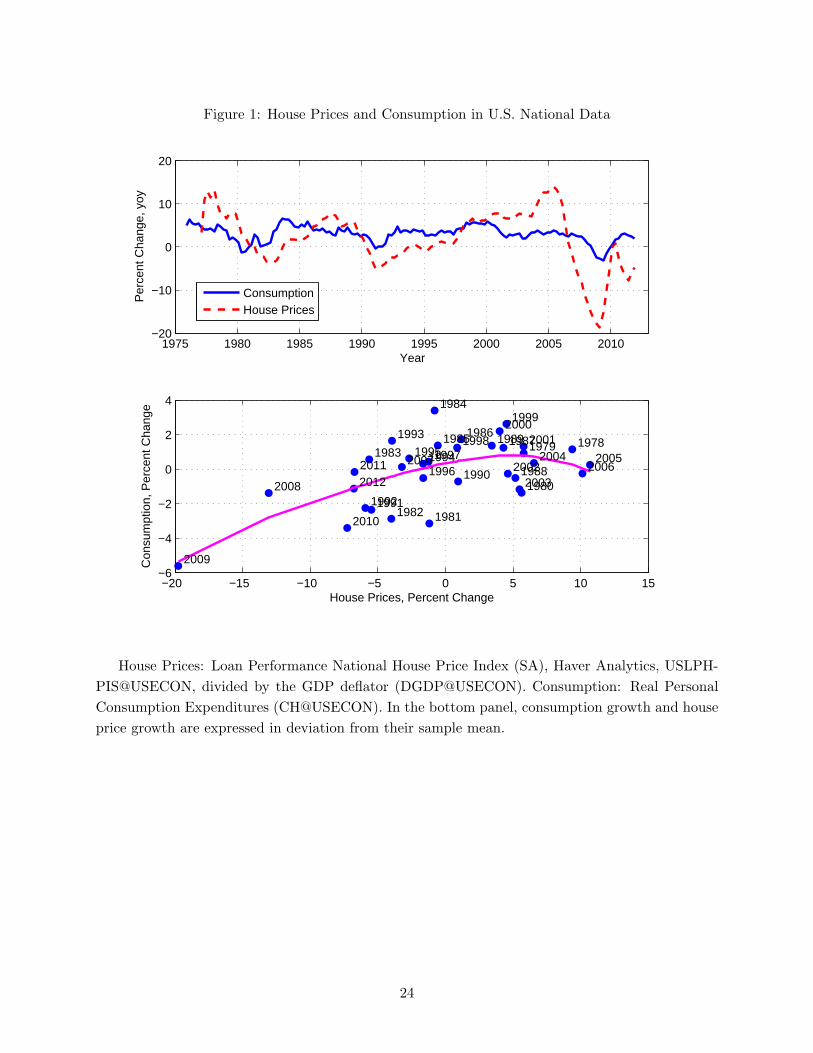
Figure 1: House Prices and Consumption in U.S. National Data

1975 1980 1985 1990 1995 2000 2005 2010−20

−10

0

10

20

Year

Per

cent

Cha

nge,

yoy

ConsumptionHouse Prices

−20 −15 −10 −5 0 5 10 15−6

−4

−2

0

2

4

House Prices, Percent Change

Con

sum

ptio

n, P

erce

nt C

hang

e

19781979

1980

19811982

1983

1984

198519861987

1988

1989

1990

19911992

1993

19941995

19961997

1998

19992000

2001

20022003

2004 200520062007

2008

2009

2010

20112012

House Prices: Loan Performance National House Price Index (SA), Haver Analytics, USLPH-

PIS@USECON, divided by the GDP deflator (DGDP@USECON). Consumption: Real Personal

Consumption Expenditures (CH@USECON). In the bottom panel, consumption growth and house

price growth are expressed in deviation from their sample mean.

24

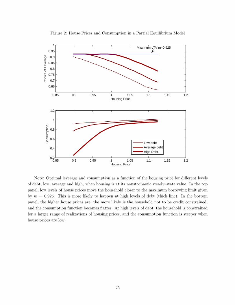
Figure 2: House Prices and Consumption in a Partial Equilibrium Model

0.85 0.9 0.95 1 1.05 1.1 1.15 1.2

0.65

0.7

0.75

0.8

0.85

0.9

0.95

1

Housing Price

Cho

ice

of L

ever

age

0.85 0.9 0.95 1 1.05 1.1 1.15 1.20.2

0.4

0.6

0.8

1

1.2

Housing Price

Con

sum

ptio

n

Low debtAverage debtHigh Debt

Maximum LTV m=0.925

Note: Optimal leverage and consumption as a function of the housing price for different levels

of debt, low, average and high, when housing is at its nonstochastic steady–state value. In the top

panel, low levels of house prices move the household closer to the maximum borrowing limit given

by m = 0.925. This is more likely to happen at high levels of debt (thick line). In the bottom

panel, the higher house prices are, the more likely is the household not to be credit constrained,

and the consumption function becomes flatter. At high levels of debt, the household is constrained

for a larger range of realizations of housing prices, and the consumption function is steeper when

house prices are low.

25

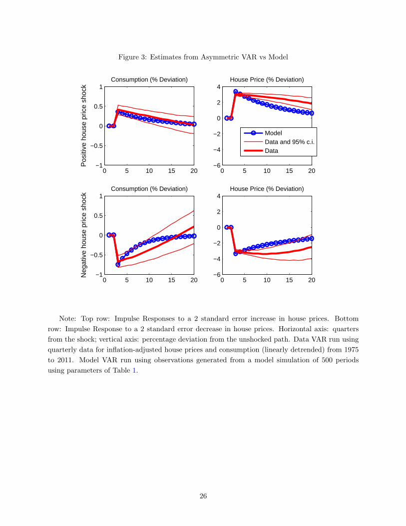
Figure 3: Estimates from Asymmetric VAR vs Model

0 5 10 15 20−1

−0.5

0

0.5

1Consumption (% Deviation)

Pos

itive

hou

se p

rice

shoc

k

0 5 10 15 20−6

−4

−2

0

2

4House Price (% Deviation)

0 5 10 15 20−1

−0.5

0

0.5

1Consumption (% Deviation)

Neg

ativ

e ho

use

pric

e sh

ock

0 5 10 15 20−6

−4

−2

0

2

4House Price (% Deviation)

ModelData and 95% c.i.Data

Note: Top row: Impulse Responses to a 2 standard error increase in house prices. Bottom

row: Impulse Response to a 2 standard error decrease in house prices. Horizontal axis: quarters

from the shock; vertical axis: percentage deviation from the unshocked path. Data VAR run using

quarterly data for inflation-adjusted house prices and consumption (linearly detrended) from 1975

to 2011. Model VAR run using observations generated from a model simulation of 500 periods

using parameters of Table 1.

26

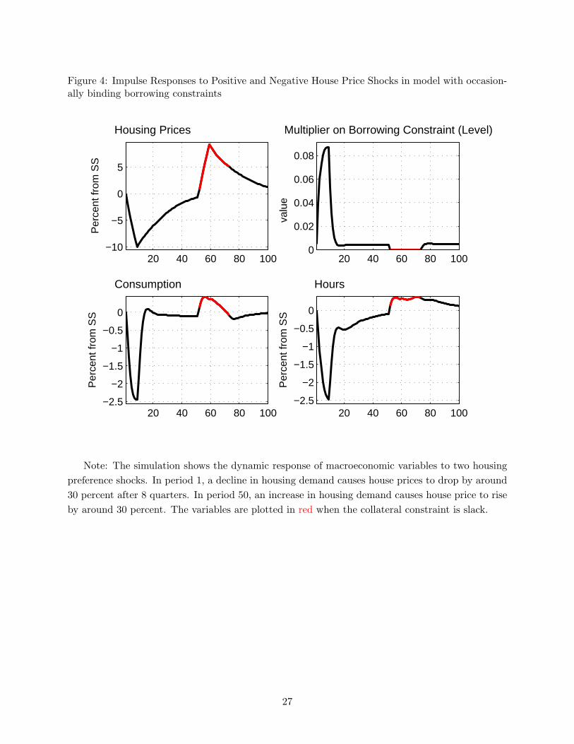
Figure 4: Impulse Responses to Positive and Negative House Price Shocks in model with occasion-ally binding borrowing constraints

20 40 60 80 100−10

−5

0

5

Housing Prices

Per

cent

from

SS

20 40 60 80 1000

0.02

0.04

0.06

0.08

Multiplier on Borrowing Constraint (Level)

valu

e

20 40 60 80 100−2.5

−2

−1.5

−1

−0.5

0

Consumption

Per

cent

from

SS

20 40 60 80 100−2.5

−2

−1.5

−1

−0.5

0

Hours P

erce

nt fr

om S

S

Note: The simulation shows the dynamic response of macroeconomic variables to two housing

preference shocks. In period 1, a decline in housing demand causes house prices to drop by around

30 percent after 8 quarters. In period 50, an increase in housing demand causes house price to rise

by around 30 percent. The variables are plotted in red when the collateral constraint is slack.

27

Figure 5: Response of Consumption to Positive and Negative Changes in Housing Prices in theDSGE model

−20 −15 −10 −5 0 5 10 15 20−6

−5

−4

−3

−2

−1

0

1

Peak Impact on Housing Prices of Housing Demand Shock (%)

Pea

k Im

pact

on

Con

sum

ptio

n (%

)

−20 −15 −10 −5 0 5 10 15 200

0.05

0.1

0.15

0.2

0.25

0.3

0.35

Peak Impact on Housing Wealth of Housing Demand Shock (%)Pea

k E

last

icity

of C

onsu

mpt

ion

to H

ousi

ng W

ealth

0 0 0 0

13

17

2022

25 27 30

# of periods borrowing constraint is relaxed

Note: The top panel plots the maximum response of consumption relative to the zero baseline

following a housing price shock of size given by the x-axis. The bottom panel plots the maximum

elasticity of consumption to housing wealth given a housing wealth shock of size given by the x-axis.

The housing price and wealth shocks are caused by a housing preference shock.

28

Figure 6: Response of Consumption to Positive and Negative Changes in Housing Prices in theDSGE model. Allowing for Zero Lower Bound

−25 −20 −15 −10 −5 0 5 10 15 20 25−8

−6

−4

−2

0

2

Peak Impact on Housing Prices of Housing Demand Shock (%)

Pea

k Im

pact

on

Con

sum

ptio

n (%

)

−25 −20 −15 −10 −5 0 5 10 15 20 250

0.05

0.1

0.15

0.2

0.25

0.3

0.35

Peak Impact on Housing Wealth of Housing Demand Shock (%)Pea

k E

last

icity

of C

onsu

mpt

ion

to H

ousi

ng W

ealth

NO ZLBZLB

Note: The top panel plots the maximum response of consumption relative to the zero baseline

following a housing price shock of size given by the x-axis, in the baseline model without zero lower

bound on nominal interest rates (NO ZLB) and in a model with the zero lower bound constraint

(ZLB). The bottom panel plots the maximum elasticity of consumption to housing wealth given a

housing wealth shock of size given by the x-axis. The housing price and wealth shocks are caused

by a housing preference shock.

29

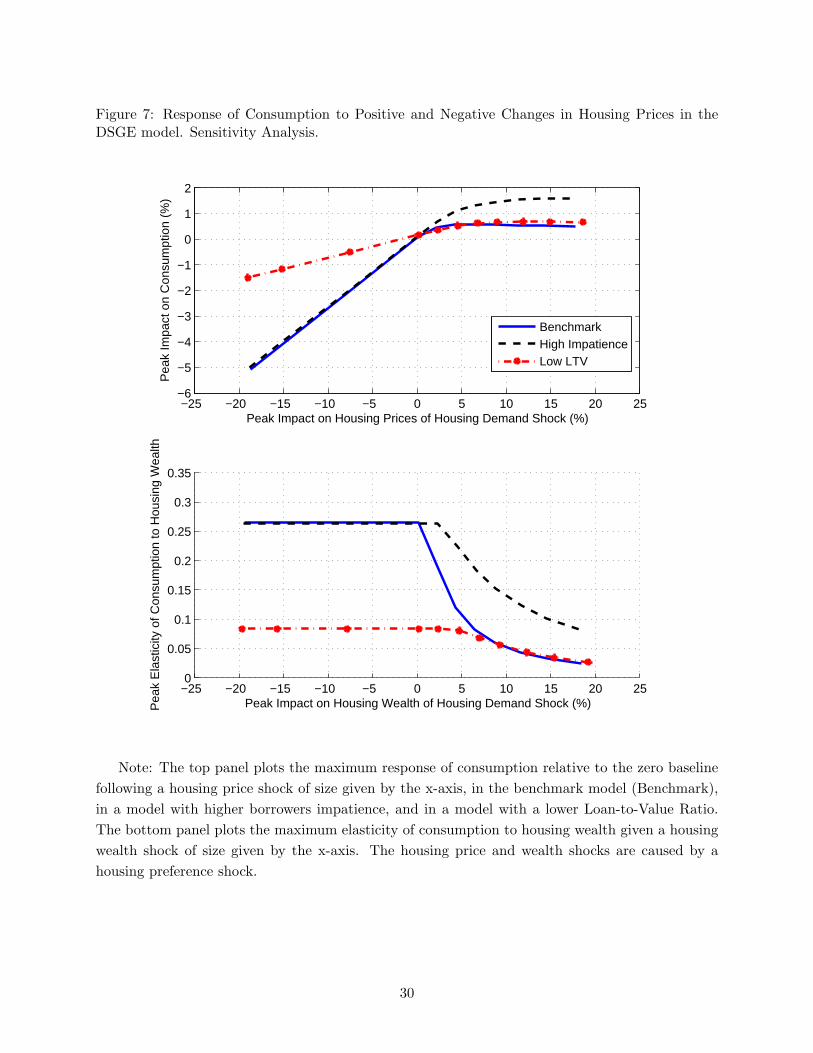
Figure 7: Response of Consumption to Positive and Negative Changes in Housing Prices in theDSGE model. Sensitivity Analysis.

−25 −20 −15 −10 −5 0 5 10 15 20 25−6

−5

−4

−3

−2

−1

0

1

2

Peak Impact on Housing Prices of Housing Demand Shock (%)

Pea

k Im

pact

on

Con

sum

ptio

n (%

)

−25 −20 −15 −10 −5 0 5 10 15 20 250

0.05

0.1

0.15

0.2

0.25

0.3

0.35

Peak Impact on Housing Wealth of Housing Demand Shock (%)Pea

k E

last

icity

of C

onsu

mpt

ion

to H

ousi

ng W

ealth

BenchmarkHigh ImpatienceLow LTV

Note: The top panel plots the maximum response of consumption relative to the zero baseline

following a housing price shock of size given by the x-axis, in the benchmark model (Benchmark),

in a model with higher borrowers impatience, and in a model with a lower Loan-to-Value Ratio.

The bottom panel plots the maximum elasticity of consumption to housing wealth given a housing

wealth shock of size given by the x-axis. The housing price and wealth shocks are caused by a

housing preference shock.

30

Figure 8: House prices and Economic Activity by State

INTX

OHCOMIKSIA

MS

OKTNNCALNEGAUT

KYSD

LA

SCMOARWVWINMND

MNILAK

IDMTWY

MANHPAORWA

MECTNYVTNJDE

AZ

VARIMD

FLDCCAHI

NV

CA

NVFLMIAZRI

MAMNNHNJMDOHCTVANYDC

ILDEWIVTCOINNE

HI

MEMOPAWVKS

GA

AK

IAARIDKYORSCMS

LA

TNALNMSD

NCWAOKTXMTNDWY

UT

−10

−5

05

% C

hang

e in

Em

ploy

men

t

−20 0 20 40Lagged one−year % change in House Prices

House Prices and Employment

INTXOHCO

MI

KSIAMSOKTNNCALNEGAUT

KYSDSCMOARWVWI

NMND

MNILAK

IDMTWY

MANHPAORWAMECTNYVTNJ

DEAZVARIMD

FL

DC

CAHI NV

CANVFLMIAZRIMAMNNHNJ

MDOHCTVANY

DC

ILDEWIVTCOINNEHIMEMOPAWVKSGAAKIAARIDKYORSCMSTNALNMSDNCWA

OKTXMTNDWY

UT

−30

−20

−10

010

% C

hang

e in

Aut

o

−20 0 20 40Lagged one−year % change in House Prices

House Prices and Auto Sales

INTXOHCO

MIKSIA

MS

OKTNNCALNE

GAUT

KYSD

LA

SC

MOAR

WVWINMNDMN

IL

AK

IDMTWYMANHPA

ORWAMECTNY

VT

NJDEAZVARI

MDFL

DC

CAHI

NVCA

NVFLMIAZRIMAMNNHNJMDOH

CT

VANYDCILDEWIVTCOINNE

HIMEMOPAWV

KSGAAKIAARID

KY

ORSCMSLATNALNM

SD

NC

WAOKTXMTNDWY

UT

−10

−5

05

10%

Cha

nge

in E

lect

ricity

−20 0 20 40Lagged one−year % change in House Prices

2005 2008 Fitted

House Prices and Electricity

INTXOHCOMIKSIAMSOKTNNCALNEGAUT

KYSDSCMOARWVWI

NMNDMNILAK

ID

MTWY

MANHPA

ORWAMECTNYVTNJDE

AZ

VARI

MDFL

DCCAHI

NV

LA

CANVFL

MIAZRIMAMNNHNJMD

OHCTVANYDCILDEWIVTCOINNE

HIMEMOPAWVKSGAAKIAAR

IDKY

ORSCMSTNAL

NM

SD

NCWA

OKTXMTND

WYUTLA

−60

−40

−20

020

40%

Cha

nge

in O

rigin

atio

ns

−20 0 20 40Lagged one−year % change in House Prices

2005 2008 Fitted

House Prices and Mortgage Originations

Note: Each panel shows house price growth and activity growth across US states in 2005 and

2008. The “fitted” line shows the fitted values of a regression of activity growth on house prices

growth broken down into positive and negative changes.

31

Figure 9: A Transfer from Lenders to Borrowers Against a Background of Low and High HousingPrices

20 40 60 80−10

−5

0

5

Housing Prices

% d

ev. f

rom

SS

20 40 60 800

0.2

0.4

0.6

0.8

1

Transfer

% o

f SS

con

sum

ptio

n

20 40 60 80

0

0.2

0.4

0.6

Consumption

% d

ev. f

rom

bas

elin

e

20 40 60 80

−0.2

−0.1

0

0.1

0.2

0.3

Hours

% d

ev. f

rom

bas

elin

e

20 40 60 80

−0.4

−0.3

−0.2

−0.1

0Consumption saver

% d

ev. f

rom

bas

elin

e

20 40 60 800

0.5

1

1.5

2

2.5

Consumption borrower

% d

ev. f

rom

bas

elin

e

Note: The figure shows the effects of two unexpected lump-sum transfers from savers to borrow-

ers each sized at 1 percent of steady-state total consumption. The first transfer (periods 10 to 19)

happens against a baseline of low house prices and tight collateral constraints. The second transfer

(periods 50 to 59) happens against a baseline of high house prices and slack collateral constraints.

Both housing price changes in the baseline stem from a housing preference shock. The responses of

consumption, hours, consumption of savers, and consumption of borrowers are shown in deviation

from the baseline to isolate the partial effect of the transfer shocks. The variables are plotted in

red when the collateral constraint is slack.

32

Table 1: Parameter Values

Parameter Value Parameter Value

ε habit saver 0.32 β discount saver 0.9925ε′ habit borrower 0.58 j housing utility weight 0.12η labor disutility saver 0.52 µc capital share, goods 0.35η′ labor disutility borrower 0.51 µh capital share, houses 0.1ξ labor substitutab. saver 0.66 µl land share, houses 0.10ξ′ labor substitutab. borrower 0.97 µb intermediates share, houses 0.10ϕk,c adj.cost, capital for goods 14.25 δh housing depreciation 0.01

ϕk,h adj.cost, capital for houses 10.90 δkc capital depreciation, goods 0.025

ρj AR(1) housing demand shock 0.96 δkh capital depreciation, houses 0.03

rπ inflation response Taylor rule 1.44 X price markup 1.15rY output response Taylor rule 0.52 Xwc wage markup, goods 1.15θp Calvo price stickiness 0.83 Xwh wage markup, houses 1.15ιπ Calvo price indexation 0.69θw,c Calvo wage stickiness goods 0.79 α savers wage share 0.60**ιw,c Calvo wage index. goods 0.08 m loan-to-value ratio 0.925**θw,h Calvo wage stickiness houses 0.91 rR inertia, Taylor rule 0.70**ιw,h Calvo wage index. houses 0.40 ρm AR(1), LTV shock 0.95*ζ Capital Utilization convexity 0.69

γAC goods technology trend 0.0032 β′ discount borrower 0.988***γAH housing technology trend 0.0008 σj st.dev housing pref. shock 0.0825***γAH investment technology trend 0.0027 σm st.dev LTV shock 0.0205***

Note: Parameters denoted with a * were not present in the original model of Iacoviello and

Neri (2010). Parameters denoted with ** are calibrated differently. Parameters denoted with ***

are estimated in Section 4.

33

Table 2: State Level: Employment in Services and House Prices

% Change in Employment (∆empt)

∆hpt−1 0.14***(0.01)

∆hp hight−1 0.07*** 0.08*** 0.03* 0.02(0.01) (0.01) (0.02) (0.01)

∆hp lowt−1 0.24*** 0.12*** 0.08*** 0.07***(0.02) (0.02) (0.02) (0.02)

∆empt−1 0.26*** 0.23***(0.08) (0.09)

∆incomet−1 0.07**(0.03)

pval difference 0.000 0.100 0.013 0.017

Time effects no no yes yes yesObservations 1071 1071 1071 1020 1020

States 51 51 51 51 51R-squared 0.12 0.16 0.66 0.72 0.73

Note: Regressions using annual observations from 1991 to 2011 on 51 States. Robust standard

errors in parenthesis. ***,**,*: Coefficients statistically different from zero at 1, 5 and 10% confi-

dence level, respectively. pval is the p-value of the test for difference between low-house price and

high-house prices coefficient.

Data Sources and Definitions: ∆hp is the inflation–adjusted (using the GDP deflator) percent

change in the FHFA House Price Index. ∆emp is the percent change in employment in the Non-

Tradeable Service Sector which includes: Retail Trade, Transportation and Utilities, Information,

Financial Activities, Professional and Business Services, Education and Health Services, Leisure and

Hospitality, and Other Services (source: BLS Current Employment Statistics: Employment, Hours,

and Earnings - State and Metro Area). ∆income is the percent change in the inflation–adjusted

state-level disposable personal income (source: Bureau of Economic Analysis).

34

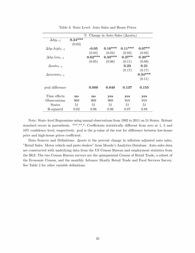
Table 3: State Level: Auto Sales and House Prices

% Change in Auto Sales (∆autot)

∆hpt−1 0.24***(0.03)

∆hp hight−1 -0.05 0.16*** 0.11*** 0.07**(0.04) (0.04) (0.03) (0.03)

∆hp lowt−1 0.62*** 0.33*** 0.27** 0.20**(0.05) (0.06) (0.11) (0.09)

∆autot−1 0.23 0.21(0.17) (0.17)

∆incomet−1 0.34***(0.11)

pval difference 0.000 0.040 0.137 0.155

Time effects no no yes yes yesObservations 969 969 969 918 918

States 51 51 51 51 51R-squared 0.02 0.06 0.86 0.87 0.88

Note: State–level Regressions using annual observations from 1992 to 2011 on 51 States. Robust

standard errors in parenthesis. ***,**,*: Coefficients statistically different from zero at 1, 5 and

10% confidence level, respectively. pval is the p-value of the test for difference between low-house

price and high-house prices coefficient.

Data Sources and Definitions: ∆auto is the percent change in inflation–adjusted auto sales,

”Retail Sales: Motor vehicle and parts dealers” from Moody’s Analytics Database. Auto sales data

are constructed with underlying data from the US Census Bureau and employment statistics from

the BLS. The two Census Bureau surveys are the quinquennial Census of Retail Trade, a subset of

the Economic Census, and the monthly Advance Montly Retail Trade and Food Services Survey.

See Table 2 for other variable definitions.

35

Table 4: State Level: Electricity Consumption and House Prices

% Change in Electricity Consumption (∆elect)

∆hpt−1 0.11***(0.02)

∆hp hight−1 0.03 0.09*** 0.14*** 0.12***(0.02) (0.02) (0.03) (0.03)

∆hp lowt−1 0.24*** 0.16*** 0.22*** 0.19***(0.03) (0.03) (0.04) (0.04)

∆elect−1 -0.41*** -0.41***(0.02) (0.02)

∆incomet−1 0.15***(0.05)

pval difference 0.000 0.105 0.058 0.090

Time effects no no yes yes yesWeather Controls* yes yes yes yes yes

Observations 1071 1071 1071 1020 1020States 51 51 51 51 51

R-squared 0.04 0.04 0.08 0.12 0.12

Note: State–level Regressions using annual observations from 1990 to 2011 on 51 States. Robust

standard errors in parenthesis. ***,**,*: Coefficients statistically different from zero at 1, 5 and

10% confidence level, respectively. pval is the p-value of the test for difference between low-house

price and high-house prices coefficient.

Data Sources and Definitions: ∆elec is the percent change in Residential Electricity Consump-

tion (source: the U.S. Energy Information Administration’s Electric Power Monthly publication.

Electricity Power Annual: Retail Sales - Total Electric Industry - Residential Sales, NSA, Megawatt-

hours). See Table 2 for other variable definitions. All regressions in the Table control separately

for number of heating and cooling degree days in each state (source: U.S. National Oceanic and

Atmospheric Administration’s National Climatic Data Center).

36

Table 5: State Level: Mortgage Originations and House Prices

% Change in Mortgage Originations (∆morit)

∆hpt−1 1.10***(0.18)

∆hp hight−1 -0.41* 1.08*** 1.46*** 1.54***(0.24) (0.16) (0.21) (0.33)

∆hp lowt−1 3.13*** 1.85*** 2.53*** 2.67**(0.59) (0.68) (0.90) (1.11)

∆morit−1 -0.20*** -0.20***(0.02) (0.02)

∆incomet−1 -0.63(1.04)

pval difference 0.000 0.211 0.160 0.181

Time effects no no yes yes yesObservations 1020 1020 1020 969 969

States 51 51 51 51 51R-squared 0.01 0.03 0.58 0.53 0.53

Note: State–level Regressions using annual observations from 1992 to 2011 on 51 States. Robust

standard errors in parenthesis. ***,**,*: Coefficients statistically different from zero at 1, 5 and

10% confidence level, respectively. pval is the p-value of the test for difference between low-house

price and high-house prices coefficient.

Data Sources and Definitions: ∆mori is the percent change in “Mortgage originations and pur-

chases: Value” from the U.S. Federal Financial Institutions Examination Council: Home Mortgage

Disclosure Act. See Table 2 for other variable definitions.

37

Table 6: MSA Level: Employment in Services and House Prices

% Change in Employment (∆empt)

∆hpt−1 0.134***(0.006)

∆hp hight−1 0.104*** 0.058*** 0.049*** 0.044***(0.008) (0.007) (0.008) (0.008)

∆hp lowt−1 0.183*** 0.099*** 0.095*** 0.089***(0.009) (0.008) (0.010) (0.010)

∆empt−1 0.033 0.026(0.041) (0.041)

∆incomet−1 0.040**(0.019)

pval difference 0.0000 0.0003 0.0001 0.0001

Time effects no no yes yes yesObservations 5390 5390 5390 5147 5147

MSA 262 262 262 262 262R-squared 0.09 0.10 0.37 0.39 0.40

Note: State–level Regressions using annual observations from 1992 to 2011 on 262 MSAs (102

MSAs were dropped since they had incomplete or missing data on employment by sector). Robust

standard errors in parenthesis. ***,**,*: Coefficients statistically different from zero at 1, 5 and

10% confidence level, respectively. pval is the p-value of the test for difference between low-house

price and high-house prices coefficient.

Data Sources and Definitions: see Table 2.

38

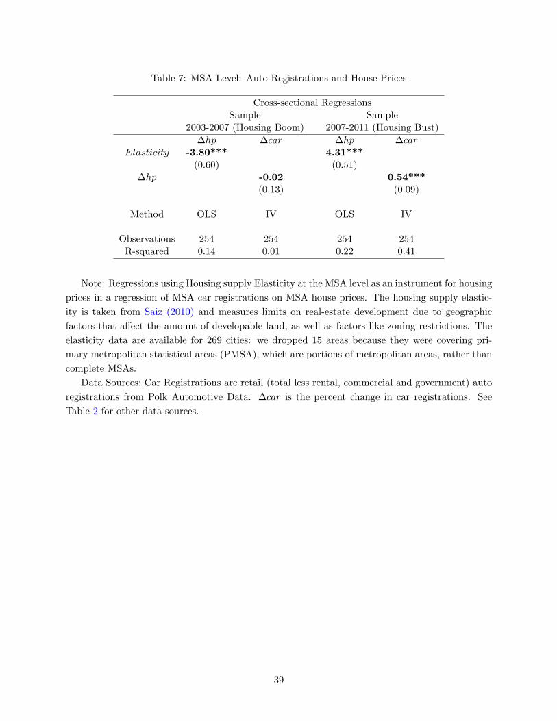
Table 7: MSA Level: Auto Registrations and House Prices

Cross-sectional RegressionsSample Sample

2003-2007 (Housing Boom) 2007-2011 (Housing Bust)

∆hp ∆car ∆hp ∆carElasticity -3.80*** 4.31***

(0.60) (0.51)∆hp -0.02 0.54***

(0.13) (0.09)

Method OLS IV OLS IV

Observations 254 254 254 254R-squared 0.14 0.01 0.22 0.41

Note: Regressions using Housing supply Elasticity at the MSA level as an instrument for housing

prices in a regression of MSA car registrations on MSA house prices. The housing supply elastic-

ity is taken from Saiz (2010) and measures limits on real-estate development due to geographic

factors that affect the amount of developable land, as well as factors like zoning restrictions. The

elasticity data are available for 269 cities: we dropped 15 areas because they were covering pri-

mary metropolitan statistical areas (PMSA), which are portions of metropolitan areas, rather than

complete MSAs.

Data Sources: Car Registrations are retail (total less rental, commercial and government) auto

registrations from Polk Automotive Data. ∆car is the percent change in car registrations. See

Table 2 for other data sources.

39