Collection of solutions to simulation problems in MT426 ... · Collection of solutions to simulation problems in MT426 (probability: random variables) using R. Aaron McMillan Fraenkel

Collection of solutions to simulation problems in MT426(probability: random variables) using R.

Aaron McMillan Fraenkel

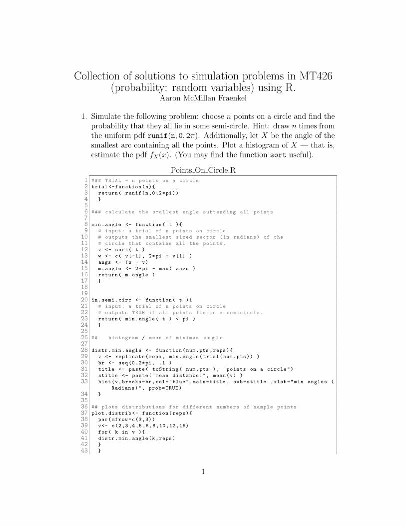
1. Simulate the following problem: choose n points on a circle and find theprobability that they all lie in some semi-circle. Hint: draw n times fromthe uniform pdf runif(n, 0, 2π). Additionally, let X be the angle of thesmallest arc containing all the points. Plot a histogram of X — that is,estimate the pdf fX(x). (You may find the function sort useful).

Points On Circle.R1 ### TRIAL = n points on a circle

2 trial <-function(n){

3 return( runif(n,0,2*pi))

4 }

56 ### calculate the smallest angle subtending all points

78 min.angle <- function( t ){

9 # input: a trial of n points on circle

10 # outputs the smallest sized sector (in radians) of the

11 # circle that contains all the points.

12 v <- sort( t )

13 w <- c( v[-1], 2*pi + v[1] )

14 angs <- (w - v)

15 m.angle <- 2*pi - max( angs )

16 return( m.angle )

17 }

181920 in.semi.circ <- function( t ){

21 # input: a trial of n points on circle

22 # outputs TRUE if all points lie in a semicircle.

23 return( min.angle( t ) < pi )

24 }

2526 ## histogram / mean of minimum a n g l e

2728 distr.min.angle <- function(num.pts ,reps){

29 v <- replicate(reps , min.angle(trial(num.pts)) )

30 br <- seq(0,2*pi, .1 )

31 title <- paste( toString( num.pts ), "points on a circle")

32 stitle <- paste("mean distance:", mean(v) )

33 hist(v,breaks=br ,col="blue",main=title , sub=stitle ,xlab="min angles (

Radians)", prob=TRUE)

34 }

3536 ## plots distributions for different numbers of sample points

37 plot.distrib <- function(reps){

38 par(mfrow=c(3,3))

39 v<- c(2,3,4,5,6,8,10,12,15)

40 for( k in v ){

41 distr.min.angle(k,reps)

42 }

43 }

1

4445 ## relative frequency of "n random points lying in a semi -circle"

46 rel.freq <- function(num.pts ,reps){

47 # relative freq of n points sitting

48 # in a semicircle

49 exper <- replicate(reps , in.semi.circ( trial(num.pts) ) )

50 return( mean( exper ) )

51 }

52 ## Plot relative frequencies for different sample sizes

53 rf.plot <- function( reps ){

54 v<-numeric (20)

55 for( k in 1:20){ v[k]<- rel.freq(k,reps)}


57 title <- "relative frequency of n points lying in a semicircle"

58 xvar <- "number of sample points n"

59 plot(v, main=title , xlab=xvar , ylab="probability" )

60 lines(v)

61 }

6263 #########################################

64 # The rest is dedicated to visually depicting the points on a circle

65 #########################################

6667 min.max <- function( t ){

68 # input a trial t

69 # outputs the two consecutive points

70 # on circle that have max angle between them.

71 v <- sort( t )

72 w <- c( v[-1], 2*pi + v[1] )

73 angs <- (w - v)

74 k <- which( angs == max(angs) )

75 if( k != length(t) ){

76 mm <- c( v[k], v[k+1] )

77 } else {

78 mm<- c(v[k], v[1] )

79 }

80 return( mm )

81 }

8283 #### Visually depict a single trial on a circle

84 gtrial <- function( v ){

85 n<- length(v)

86 if( in.semi.circ( v ) == TRUE ){ s<- "Fits in a Semicircle"}else{s<- "

Doesn ’t fit in a Semicircle"}

87 mina <- paste("angle = ", min.angle( v ) )

88 plot(cos(v),sin(v),xlim=c(-1,1),ylim=c(-1,1),col="red", main=s,ylab=""

,xlab=mina )

89 curve(sqrt(1-x^2),add=T)

90 curve(-sqrt(1-x^2),add=T)

91 for(k in 1:n){

92 if( cos(v[k]) < 0 ){

93 bmin <-cos(v[k])

94 bmax <- 0

95 } else {

96 bmin <-0

97 bmax <-cos(v[k])

98 }

99 curve(x*sin(v[k])/cos(v[k]),from=bmin , to=bmax , add=T)

100 }

101 }

2

102 #### Attempt #2: using shapes package

103104105106 #### Illustrates 9 trials on the circle and states if

107 #### They are in a semi -circle or not.

108109 plot.trials <- function( num.pts ){


111 for(k in 1:9){ gtrial( trial( num.pts )) }

112 }

113114115 plot.trials (4)

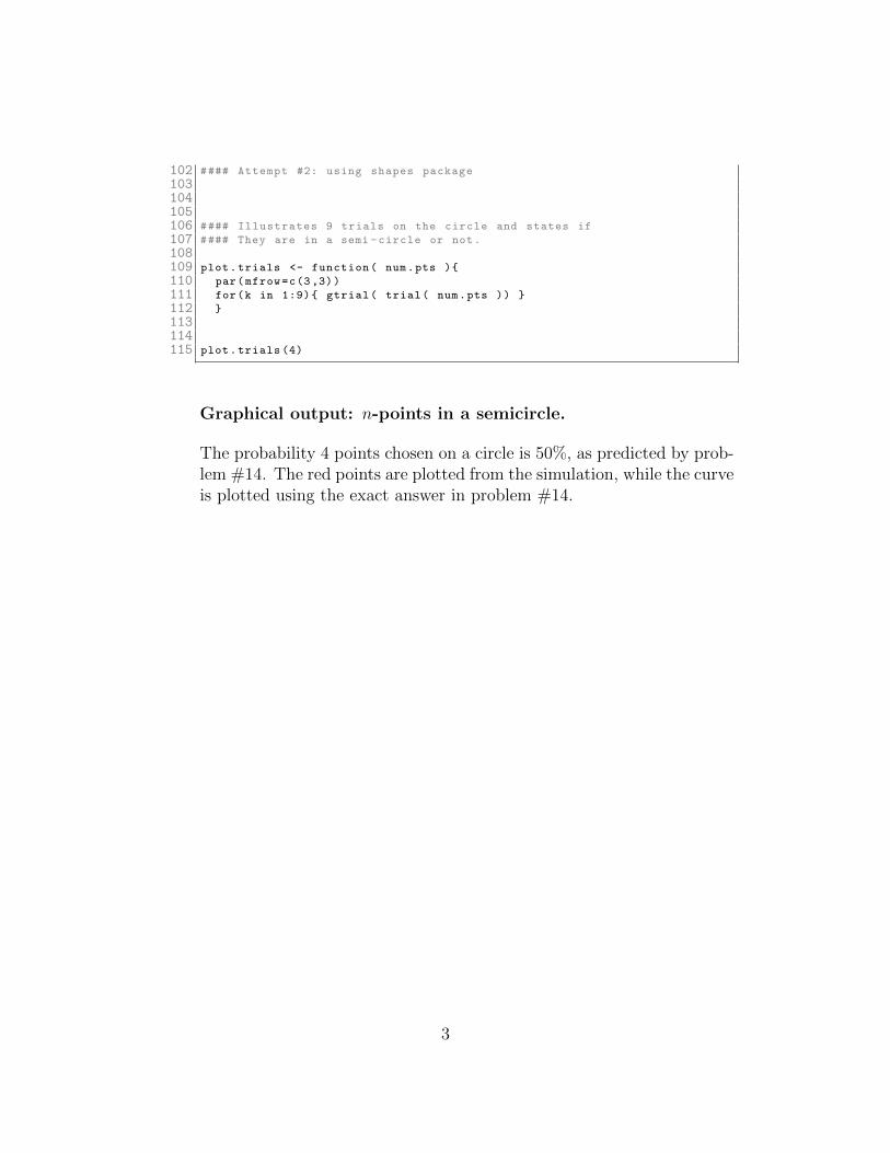
Graphical output: n-points in a semicircle.

The probability 4 points chosen on a circle is 50%, as predicted by prob-lem #14. The red points are plotted from the simulation, while the curveis plotted using the exact answer in problem #14.

3

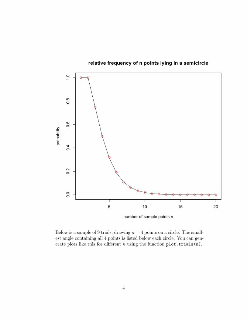
Below is a sample of 9 trials, drawing n = 4 points on a circle. The small-est angle containing all 4 points is listed below each circle. You can gen-erate plots like this for different n using the function plot.trials(n).

4

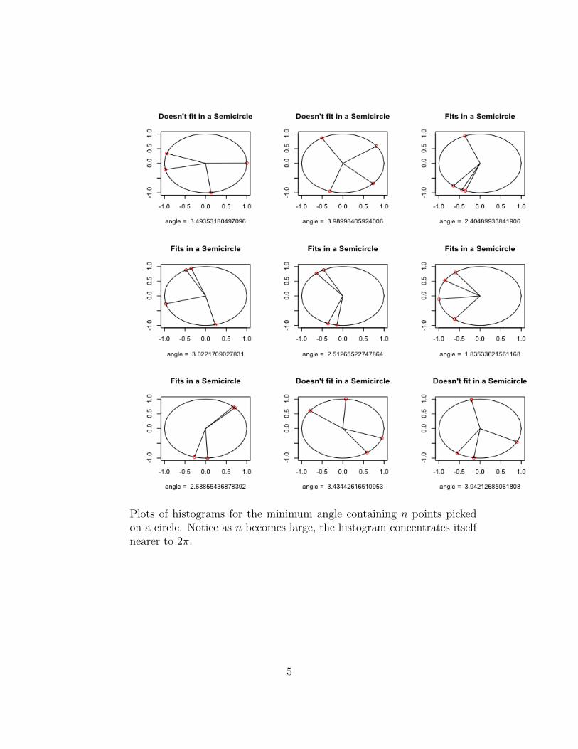
Plots of histograms for the minimum angle containing n points pickedon a circle. Notice as n becomes large, the histogram concentrates itselfnearer to 2π.

5

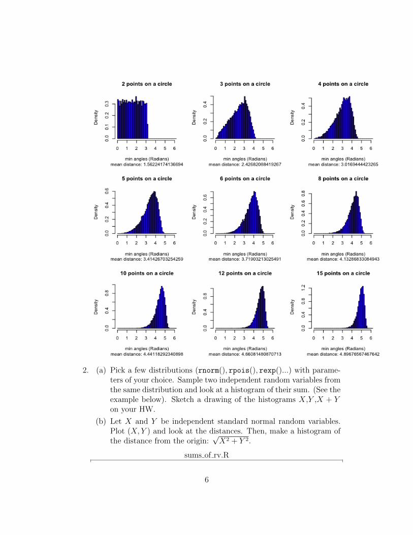
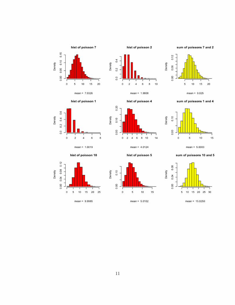
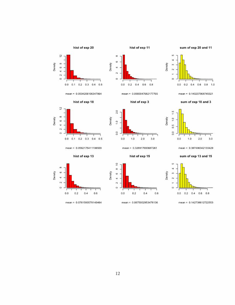
2. (a) Pick a few distributions (rnorm(), rpois(), rexp()...) with parame-ters of your choice. Sample two independent random variables fromthe same distribution and look at a histogram of their sum. (See theexample below). Sketch a drawing of the histograms X,Y ,X + Yon your HW.

(b) Let X and Y be independent standard normal random variables.Plot (X, Y ) and look at the distances. Then, make a histogram ofthe distance from the origin:

√X2 + Y 2.

sums of rv.R

6

123 ## For sums of two uniform RVs

4 ## with parameters [a,b] and [c,d].

56 unif.plot <- function(u){

7 x <- runif (10000 ,u[1],u[2])

8 m <- mean(x)

9 title <- paste("hist of unif [", toString(u), "]" )

10 stitle <- paste("mean = ", toString(m) )

11 hist(x,col="red",prob=TRUE , main=title , sub=stitle , xlab="")

1213 }

1415 unif.sum <- function(u1 ,u2){

16 # u1 = c(a,b) is parameter of uniform rv1

17 # u2 = c(c,d) is parameter of uniform rv2

18 x <- runif (10000 ,u1[1],u1[2])

19 y <- runif (10000 ,u2[1],u2[2])

20 s<- x+y

21 m <- mean(s)

22 title <- paste("sum of unif [", toString(u1), "] and [", toString(u2),

"]" )


24 hist(s,col="yellow",prob=TRUE , main=title , sub=stitle , xlab="")

2526 }

272829 sample.unif <- function (){


31 for( k in 1:3 ){

32 u1=sort( sample (0:10 ,2) )

33 u2=sort( sample (0:10 ,2) )

34 unif.plot(u1)

35 unif.plot(u2)

36 unif.sum(u1,u2)

37 }

38 }

394041424344 ## For sums of two poisson RVs with

45 ## parameters lambda1 ,lambda2.

4647 poisson.plot <-function(lambda){

48 x <- rpois (10000 , lambda)

49 m <- mean(x)

50 title <- paste("hist of poisson", toString(lambda))



5354 }

5556 poisson.sum <- function(lambda1 ,lambda2){

57 x <- rpois (10000 , lambda1)

58 y <- rpois (10000 , lambda2)

59 s<- x+y

7

60 m <- mean(s)

61 title <- paste("sum of poissons", toString(lambda1), "and", toString(

lambda2))



6465 }

666768 sample.poisson <- function (){


70 for( k in 1:3 ){

71 lambda1=sample (1:10 ,1)


73 poisson.plot(lambda1)

74 poisson.plot(lambda2)

75 poisson.sum(lambda1 ,lambda2)

76 }

77 }

787980 sample.poisson ()

818283848586 ## For sums of two exponential RVs with

87 ## waiting times lambda1 , lambda2.

8889 exp.plot <-function(lambda){

90 x <- rexp (10000 , lambda)

91 m <- mean(x)

92 title <- paste("hist of exp", toString(lambda))



9596 }

9798 exp.sum <- function(lambda1 ,lambda2){

99 x <- rexp (10000 , lambda1)

100 y <- rexp (10000 , lambda2)

101 s<- x+y

102 m <- mean(s)

103 title <- paste("sum of exp", toString(lambda1), "and", toString(

lambda2))



106107 }

108109110 sample.exp <- function (){


112 for( k in 1:3 ){



115 exp.plot(lambda1)

116 exp.plot(lambda2)

117 exp.sum(lambda1 ,lambda2)

8

118 }

119 }

120121122 sample.exp()

123124125126127 ## For the RV Z=sqrt(X^2+Y^2), that ’s the

128 ## distance from the origin of a point

129 ## (X,Y), where both are normally distributed.

130131 norm2D <- function (){


133 x<-rnorm (10000) # x-coordinate

134 y<-rnorm (10000) # y-coordinate

135 thin.ind <- sample (1:10000 ,500) # a sample of the coordinates to plot

136 plot(x[thin.ind],y[thin.ind],xlab="x coord",ylab="y coord",main="plot

of bivariate std normal in plane")

137 d <- sqrt(x^2+y^2)

138 m <- mean(d)

139 title <- "distance of bivariate std normal to (0,0)"


141 hist(d,col="red",prob=TRUE , main=title , sub=stitle , xlab="")

142 }

143144145 norm2D ()

Graphical Output: sums of random variables

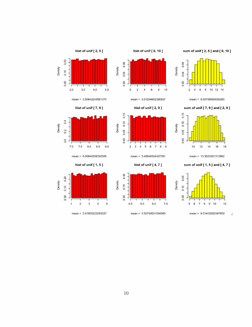
First two columns are histograms of samples of uniform random variablesX and Y . The 3rd column is the histogram of the sum. The parame-ters are randomly generated using the function sample.unif( ) . Thefollowing pages are similar.

9

10

11

12

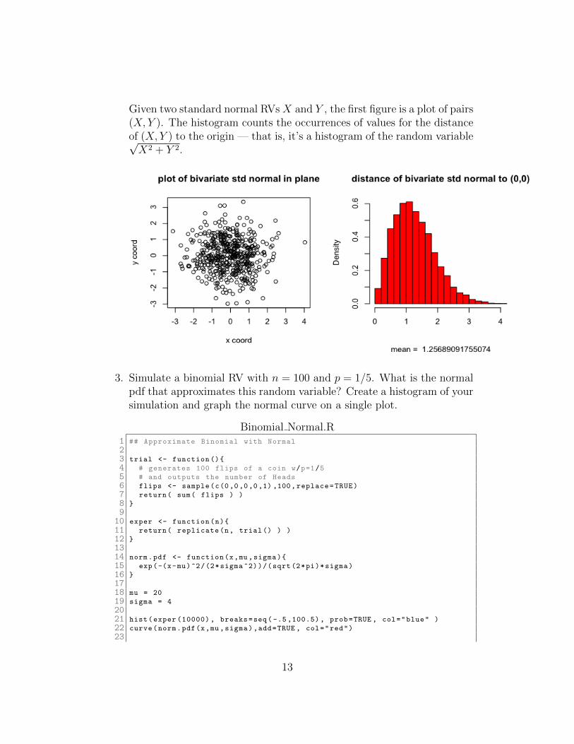
Given two standard normal RVs X and Y , the first figure is a plot of pairs(X, Y ). The histogram counts the occurrences of values for the distanceof (X, Y ) to the origin — that is, it’s a histogram of the random variable√X2 + Y 2.

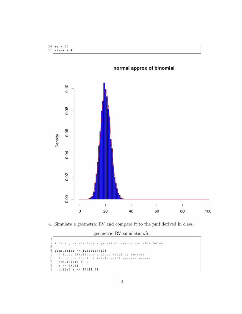
3. Simulate a binomial RV with n = 100 and p = 1/5. What is the normalpdf that approximates this random variable? Create a histogram of yoursimulation and graph the normal curve on a single plot.

Binomial Normal.R1 ## Approximate Binomial with Normal

23 trial <- function (){

4 # generates 100 flips of a coin w/p=1/5

5 # and outputs the number of Heads

6 flips <- sample(c(0,0,0,0,1) ,100,replace=TRUE)

7 return( sum( flips ) )

8 }

910 exper <- function(n){

11 return( replicate(n, trial() ) )

12 }

1314 norm.pdf <- function(x,mu,sigma){

15 exp(-(x-mu)^2/(2*sigma ^2))/(sqrt(2*pi)*sigma)

16 }

1718 mu = 20

19 sigma = 4

2021 hist(exper (10000) , breaks=seq ( -.5 ,100.5), prob=TRUE , col="blue" )

22 curve(norm.pdf(x,mu ,sigma),add=TRUE , col="red")

23

13

24 mu = 20

25 sigma = 4

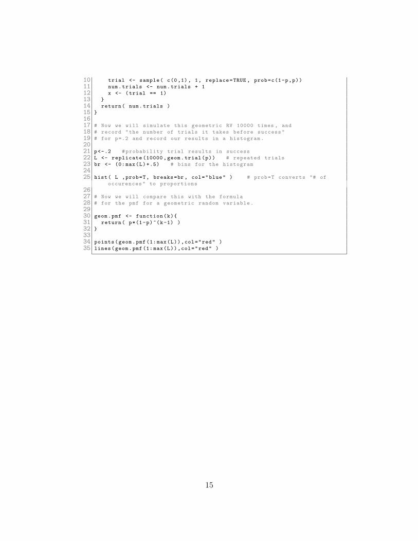
4. Simulate a geometric RV and compare it to the pmf derived in class.

geometric RV simulation.R12 # First , we simulate a geometric random variable below:

34 geom.trial <- function(p){

5 # input likelihood a given trial is success

6 # outputs the # of trials until success occurs

7 num.trials <- 0

8 x <- FALSE

9 while( x == FALSE ){

14

10 trial <- sample( c(0,1), 1, replace=TRUE , prob=c(1-p,p))

11 num.trials <- num.trials + 1

12 x <- (trial == 1)

13 }

14 return( num.trials )

15 }

1617 # Now we will simulate this geometric RV 10000 times , and

18 # record "the number of trials it takes before success"

19 # for p=.2 and record our results in a histogram.

2021 p<-.2 #probability trial results in success

22 L <- replicate (10000 , geom.trial(p)) # repeated trials

23 br <- (0:max(L)+.5) # bins for the histogram

2425 hist( L ,prob=T, breaks=br , col="blue" ) # prob=T converts "# of

occurences" to proportions

2627 # Now we will compare this with the formula

28 # for the pmf for a geometric random variable.

2930 geom.pmf <- function(k){

31 return( p*(1-p)^(k-1) )

32 }

3334 points(geom.pmf (1:max(L)),col="red" )

35 lines(geom.pmf(1: max(L)),col="red" )

15

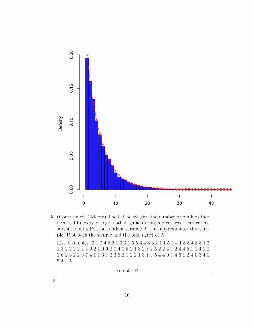
5. (Courtesy of T Moore) The list below give the number of fumbles thatoccurred in every college football game during a given week earlier thisseason. Find a Poisson random variable X that approximates this sam-ple. Plot both the sample and the pmf fX(x) of X.

List of fumbles: 3 1 2 4 6 2 1 3 3 1 5 5 4 4 3 3 2 1 1 5 2 4 1 3 3 4 3 3 1 21 3 2 2 2 2 2 3 0 2 1 0 0 2 0 4 0 5 2 1 3 2 3 2 5 2 2 4 1 2 4 4 5 1 1 4 1 21 6 2 3 2 2 0 7 4 1 1 3 1 2 3 5 2 1 2 2 1 3 1 3 5 4 4 0 1 4 6 1 2 4 0 3 4 15 4 3 5

Fumbles.R12

16

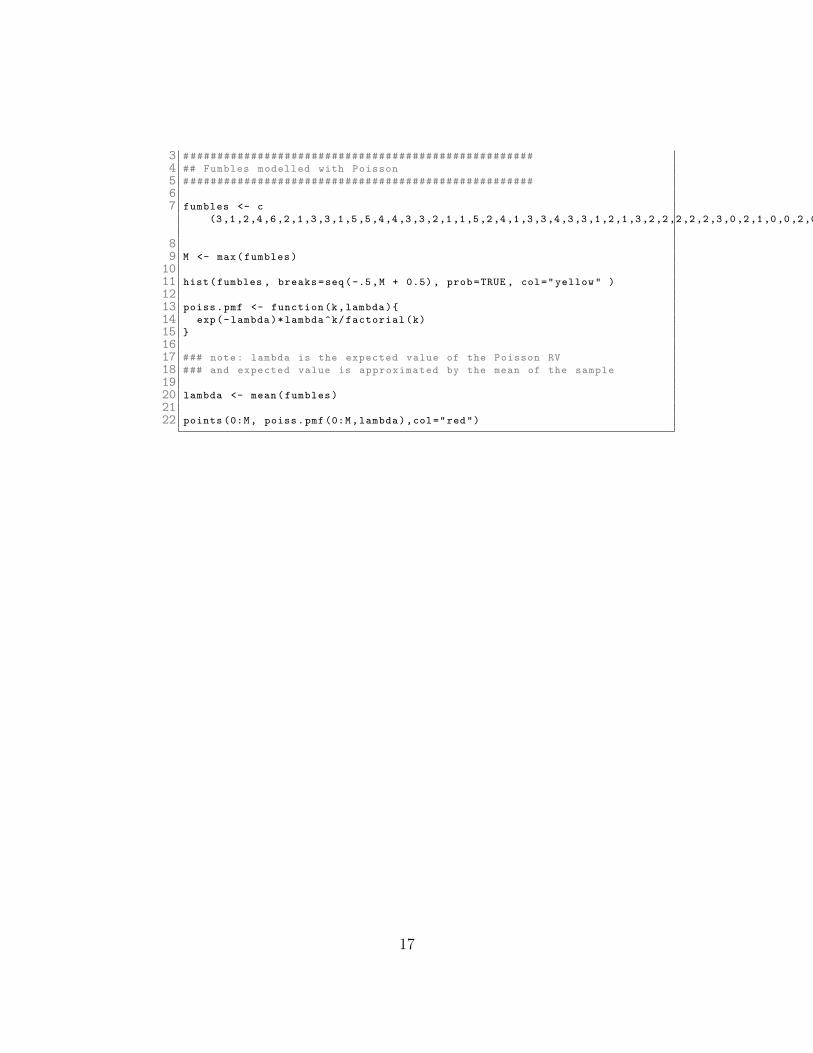
3 ####################################################

4 ## Fumbles modelled with Poisson

5 ####################################################

67 fumbles <- c

(3,1,2,4,6,2,1,3,3,1,5,5,4,4,3,3,2,1,1,5,2,4,1,3,3,4,3,3,1,2,1,3,2,2,2,2,2,3,0,2,1,0,0,2,0,4,0,5,2,1,3,2,3,2,5,2,2,4,1,2,4,4,5,1,1,4,1,2,1,6,2,3,2,2,0,7,4,1,1,3,1,2,3,5,2,1,2,2,1,3,1,3,5,4,4,0,1,4,6,1,2,4,0,3,4,1,5,4,3,5)

89 M <- max(fumbles)

1011 hist(fumbles , breaks=seq(-.5,M + 0.5), prob=TRUE , col="yellow" )

1213 poiss.pmf <- function(k,lambda){

14 exp(-lambda)*lambda^k/factorial(k)

15 }

1617 ### note: lambda is the expected value of the Poisson RV

18 ### and expected value is approximated by the mean of the sample

1920 lambda <- mean(fumbles)

2122 points (0:M, poiss.pmf(0:M,lambda),col="red")

17

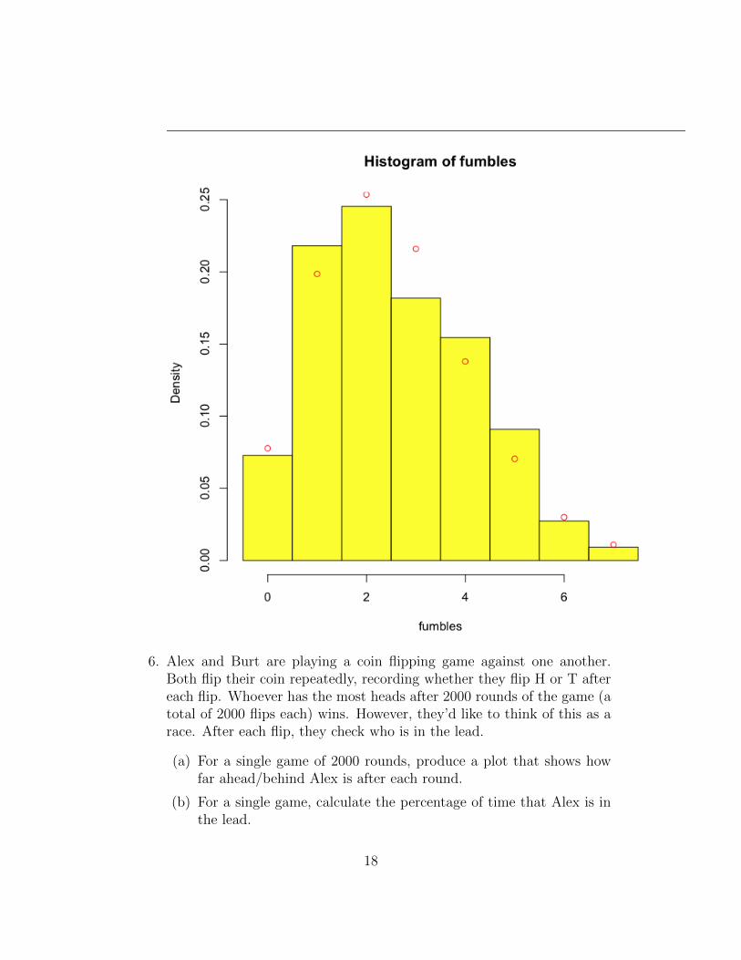
6. Alex and Burt are playing a coin flipping game against one another.Both flip their coin repeatedly, recording whether they flip H or T aftereach flip. Whoever has the most heads after 2000 rounds of the game (atotal of 2000 flips each) wins. However, they’d like to think of this as arace. After each flip, they check who is in the lead.

(a) For a single game of 2000 rounds, produce a plot that shows howfar ahead/behind Alex is after each round.

(b) For a single game, calculate the percentage of time that Alex is inthe lead.

18

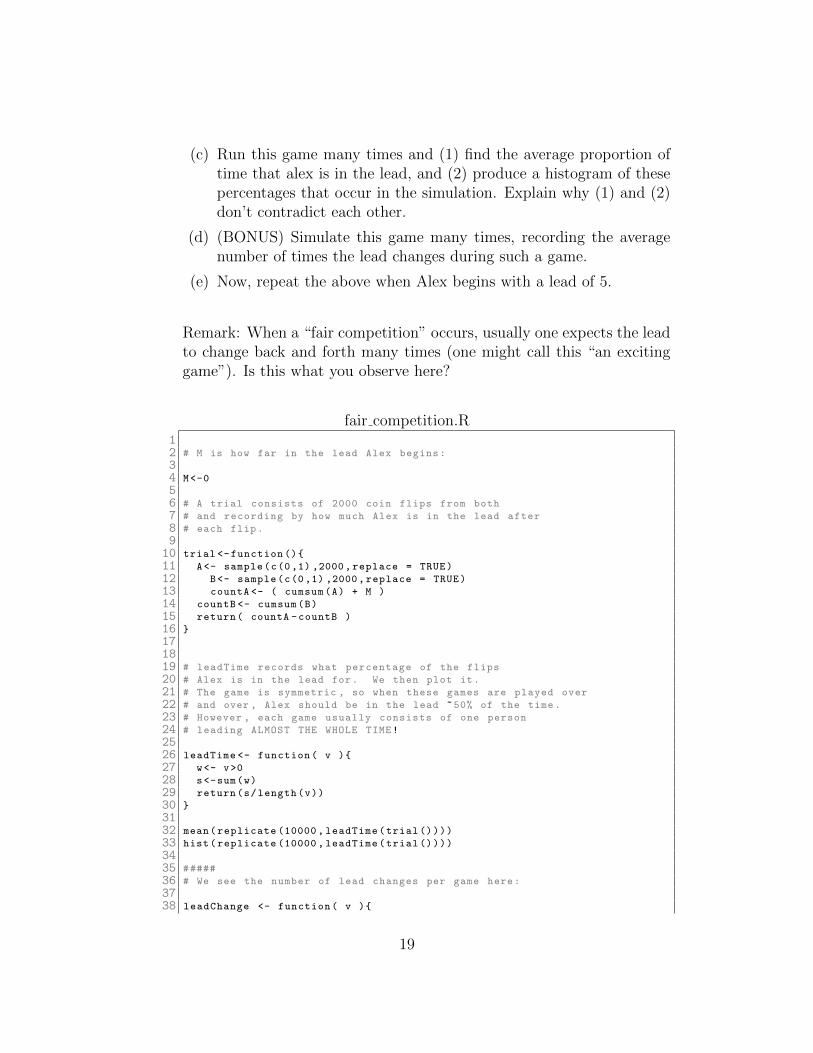
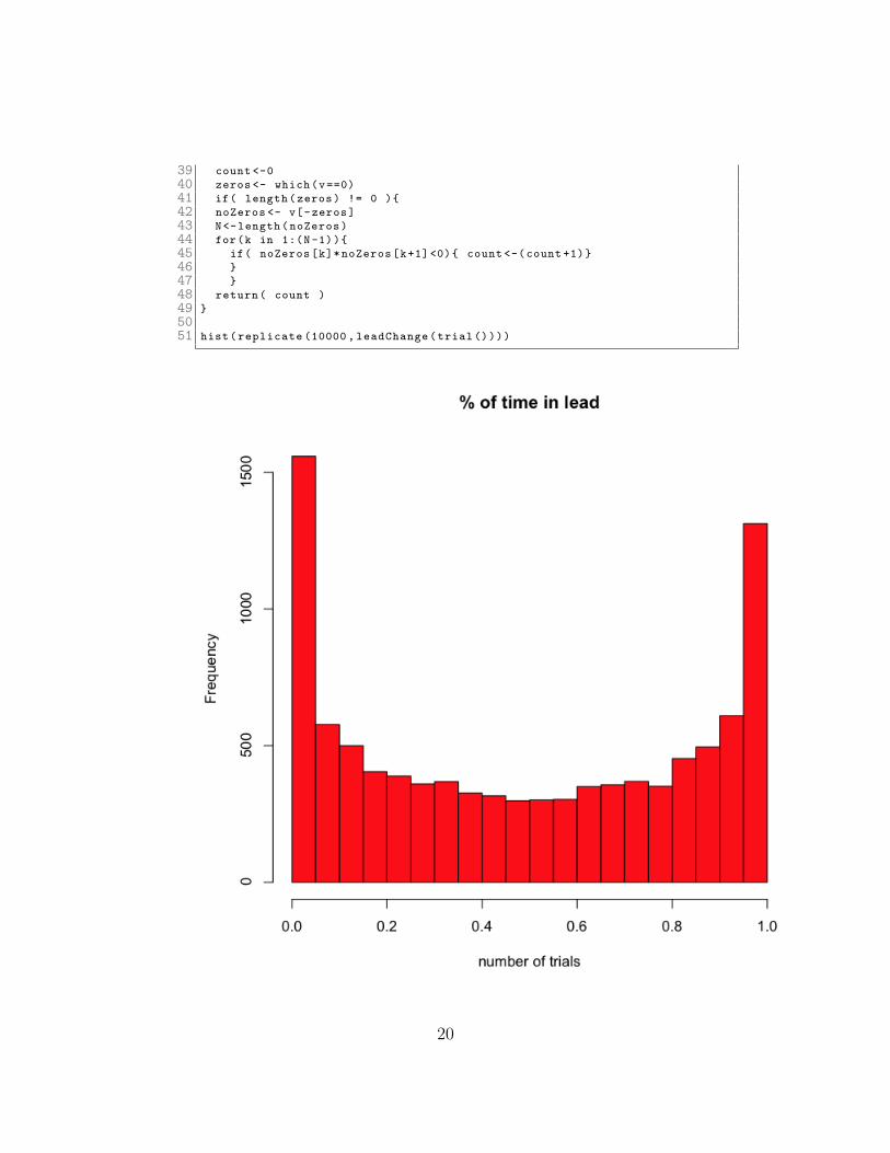
(c) Run this game many times and (1) find the average proportion oftime that alex is in the lead, and (2) produce a histogram of thesepercentages that occur in the simulation. Explain why (1) and (2)don’t contradict each other.

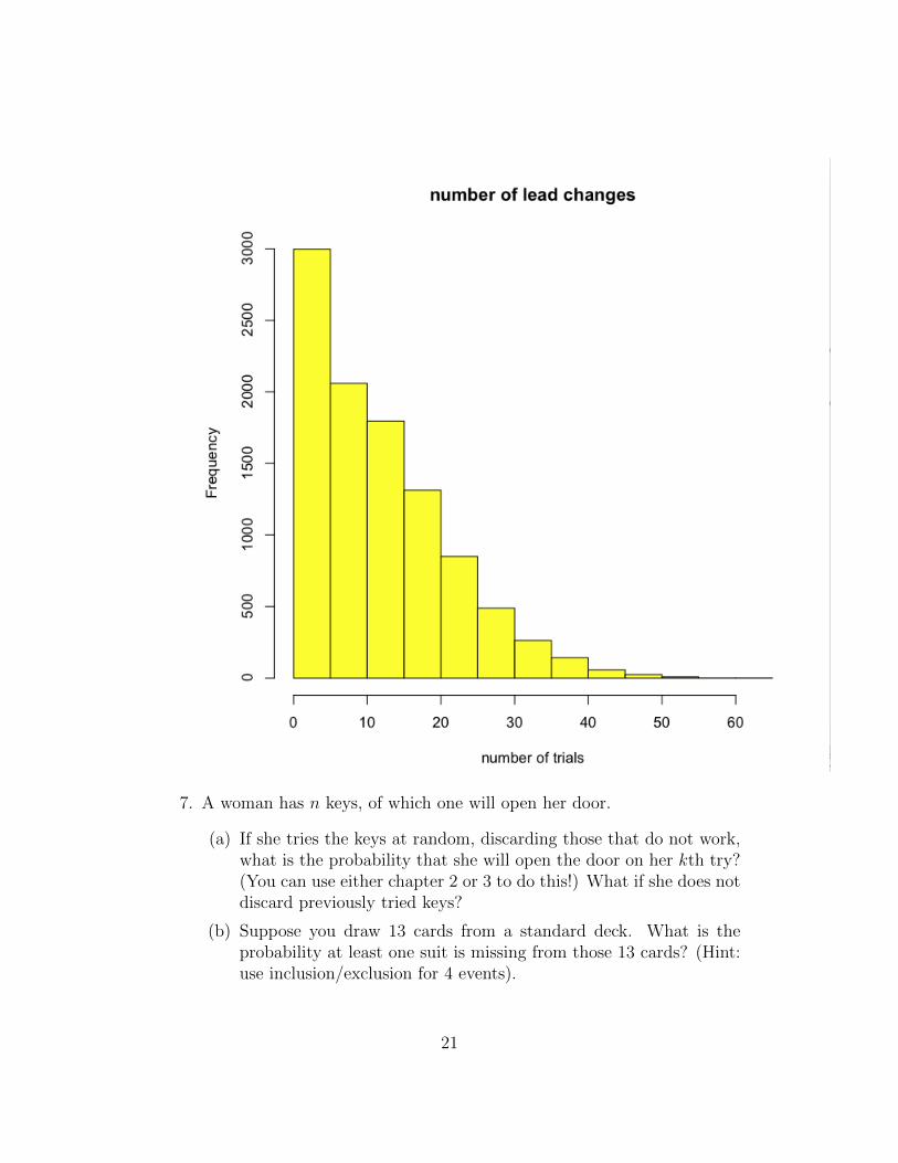
(d) (BONUS) Simulate this game many times, recording the averagenumber of times the lead changes during such a game.

(e) Now, repeat the above when Alex begins with a lead of 5.

Remark: When a “fair competition” occurs, usually one expects the leadto change back and forth many times (one might call this “an excitinggame”). Is this what you observe here?

fair competition.R12 # M is how far in the lead Alex begins:

34 M<-0

56 # A trial consists of 2000 coin flips from both

7 # and recording by how much Alex is in the lead after

8 # each flip.

910 trial <-function (){

11 A<- sample(c(0,1) ,2000, replace = TRUE)

12 B<- sample(c(0,1) ,2000, replace = TRUE)

13 countA <- ( cumsum(A) + M )

14 countB <- cumsum(B)

15 return( countA -countB )

16 }

171819 # leadTime records what percentage of the flips

20 # Alex is in the lead for. We then plot it.

21 # The game is symmetric , so when these games are played over

22 # and over , Alex should be in the lead ~50% of the time.

23 # However , each game usually consists of one person

24 # leading ALMOST THE WHOLE TIME!

2526 leadTime <- function( v ){

27 w<- v>0

28 s<-sum(w)

29 return(s/length(v))

30 }

3132 mean(replicate (10000 , leadTime(trial())))

33 hist(replicate (10000 , leadTime(trial())))

3435 #####

36 # We see the number of lead changes per game here:

3738 leadChange <- function( v ){

19

39 count <-0

40 zeros <- which(v==0)

41 if( length(zeros) != 0 ){

42 noZeros <- v[-zeros]

43 N<-length(noZeros)

44 for(k in 1:(N-1)){

45 if( noZeros[k]*noZeros[k+1]<0){ count <-(count +1)}

46 }

47 }

48 return( count )

49 }

5051 hist(replicate (10000 , leadChange(trial ())))

20

7. A woman has n keys, of which one will open her door.

(a) If she tries the keys at random, discarding those that do not work,what is the probability that she will open the door on her kth try?(You can use either chapter 2 or 3 to do this!) What if she does notdiscard previously tried keys?

(b) Suppose you draw 13 cards from a standard deck. What is theprobability at least one suit is missing from those 13 cards? (Hint:use inclusion/exclusion for 4 events).

21

discarded key.R123 ############

4 ### Question 1

5 ############

67 ##

8910 ## we make key number 1 the correct key

1112 trial1 <-function(n){return( sample (1:n,n) )} #sample of n keys

13 question1 <-function(k,t ){return( t[k]==1 )} #whether she gets the right

key on the kth try

1415 exper1 <- function(k,n,r){ return( replicate(r,question1(k,trial1(n))))}

1617 prob1 <- function(k,n,r) {return( mean(exper1(k,n,r)) )} #probability

that she opens the door on the kth try

1819 # we plot the probability for all tries and see that it’s 1/n

20 # for this we fix 20 keys!

2122 L1<-numeric (20)

23 for(k in 1:20){ L1[k]<-prob1(k,20 ,10000)}

24 plot(L1 ,ylim=c(0,1), col="blue",main="without replacement (20 keys)",

xlab="kth try worked", ylab="probability key worked")

25 curve (.05*(x/x), add=T,col="red") # plot of exact probabilities

2627 ####################

2829 trial2 <-function(k,n){return( sample (1:n,k,replace=TRUE) )} #sample of

n keys and k tries

3031 question2 <-function(k,t ){ return(t[k]==1 & sum( t[1:k]==1 ) ==1 )} #

whether she gets the right key on the kth try and not before!

3233 exper2 <- function(k,n,r){ return( replicate(r,question2(k,trial2(k,n))))

}

3435 prob2 <- function(k,n,r) {return( mean(exper2(k,n,r)) )} #probability

that she opens the door on the kth try

3637 # we plot the sample plot as before , this time w/replacement:

3839 L2<-numeric (20)

40 for(k in 1:20){ L2[k]<-prob2(k,20 ,10000)}

41 plot(L2 ,ylim=c(0,1), col="blue",main="with replacement (20 keys)", xlab=

"kth try worked", ylab="probability key worked")

42 curve ((1/20)*(19/20)^(x-1), add=T,col="red") # plot of exact

probabilities

4344 # Though , with replacement is more interesting when there are fewer keys

45 # and more tries than number of keys:

4647 L3<-numeric (20)

48 for(k in 1:20){ L3[k]<-prob2(k,3 ,10000)}

49 plot(L3 ,ylim=c(0,1), col="blue",main="with replacement (3 keys)", xlab="

kth try worked", ylab="probability key worked")

22

50 curve ((1/3)*(2/3)^(x-1), add=T,col="red")

51525354 ####################

55 # Note: question2 is not the "most intuitive" way

56 # to define whether she gets the correct key / and not before.

57 # this is an alternate way of defining it.

58 # (you could also write a more direct for loop!)

5960 first.elements <-function(k,v){

61 #input a number k and a vector

62 #outputs the first k elements of v

63 ans <-numeric(k) # start with a vector of k zeros

64 for( i in 1:k ){ ans[i]<-v[i] } # change ans to v

65 return( ans )

66 }

6768 question2 <-function(k,t){

69 iskey <- t[k]==1

70 firstkeys <- first.elements(k-1,t) # first k-1 tries to open

71 not.open.before <- sum( firstkeys == 1) == 0

72 return( sum( c(iskey ,not.open.before) ) == 2 )

73 }

747576 ## Question 2

77 ## How often is a bridge hand void in at least one suit?

7879 hearts <- replicate (13,’H’)

80 clubs <- replicate (13,’C’)

81 spades <- replicate (13,’S’)

82 diamonds <- replicate (13,’D’)

8384 deck <- c(hearts ,clubs ,spades ,diamonds)


87 return( sample(deck ,13) )

88 }

8990 question <- function( t ){

91 return( length( unique( t )) < 4 )

92 }

9394 exper <-function( n ){

95 return( replicate(n,question(trial())))

96 }

9798 rel.freq <- function( n ){

99 return( mean(exper(n))) }

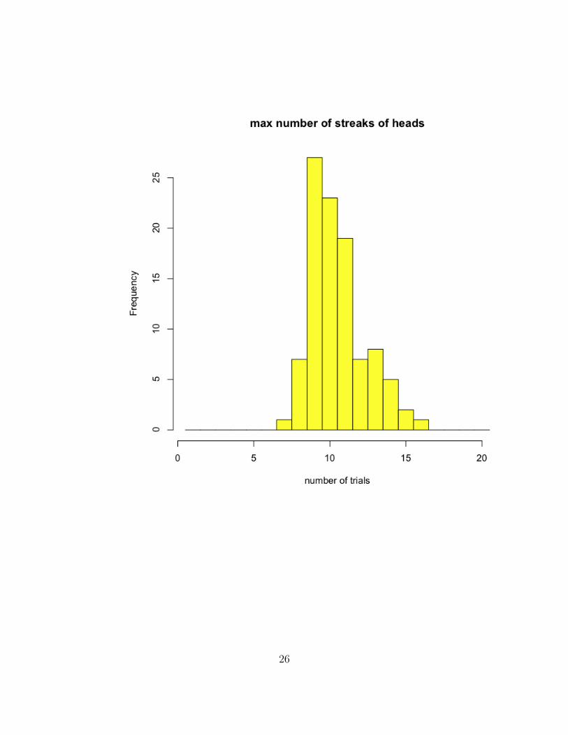
8. (a) Set up the following trial: flip a coin N = 2000 times and record the“largest streak of heads” that occurs during those flips. Repeat thistrial k times and compute the average of your results. (As k →∞,this average converges to what’s called “the expected value” of thelength of the longest streak).

23

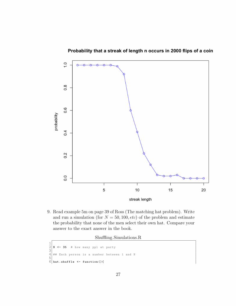
(b) Given a number n, estimate (using simulation) the probability thata streak of n heads appears in N = 2000 coin flips?

coin streaks.R12 N <- 2000

34 ## trial = N coin flips

56 flips <- function (){

7 # no input

8 # outputs N coin flips

9 # Heads = 1 / Tails = 0

10 return( sample(c(0,1),N,replace=TRUE))

11 }

1213 ## now we count the streaks at each point

14 ## in the a trial (given by flips() ).

1516 streak <- function( trial ){

17 # inputs a vector of 0/1 of length N

18 # outputs a vector w/current streak count

19 L <- numeric(N)

20 L[1] <- trial [1]

21 for ( k in 2:N ) {

22 if ( trial[k] == 1 ) { L[k] <- L[k -1]+1

23 } else { L[k] <- 0

24 }

25 }

26 return( L )

27 }

2829 ## take the max streak present in a trial:

3031 max.streak <- function( trial ){

32 # inputs a trial

33 # outputs the max streak of HEADS

34 return( max(streak( trial )))

35 }

3637 ## replicate the trial (N=2000 coin flips) and

38 ## record the max streak each time

3940 exper <- function( n ){

41 return( replicate(n, max.streak(flips()) ))

42 }

4344 # now record the average length of the max streak

45 # and view histogram of all the max streaks

4647 mean(exper (100))

48 hist(exper (100),breaks=seq (.5 ,20.5),col=’yellow ’)

49505152 ########################

53 ########################

5455 ## what is the probability there is

24

56 ## a streak of length n in N=2000 coin flips?

5758 ## here choose K=100 trials to perform the N=2000 coin flips

59 ## and ask each time: " was there a streak of length n?"

6061 K<-100

6263 hundred.trials <- function( n ){

64 # input n = length of streak

65 # outputs K=100 trials of N coin flips

66 # TRUEs if a streak of length n occurs

67 L<- replicate(K, max.streak(flips()) > n )

68 return( L )

69 }

7071 ## count up the relatively frequencies

72 ## and plot , for each n=1...20 , the relative freqs.

7374 rel.freq <- function( n ){

75 return( sum( hundred.trials(n))/K )

76 }

7778 L<-numeric (20)

79 for (k in 1:20) L[k]<- rel.freq(k)

8081 plot(L,type=’o’,col=’blue’, main=’Probability that a streak of length n

occurs in 2000 flips of a coin’,xlab=’streak length ’,ylab=’

probability ’)

828384 ############################

85 ############################

8687 ## Bonus: how many flips does it take to hit

88 ## a streak of n heads?

8990 # Notice the ‘‘while loop ’’ in the solution!

9192 str.time <- function( n ){

93 # input length of streak

94 # outputs number of flips until

95 # a streak of length n is reached

96 str.count <- 0

97 flip.count <- 0

98 while ( 0 < 1 ){

99 flip <- sample( c(0,1), 1)

100 flip.count <- flip.count + 1

101 if ( flip == 1 ) { str.count <- str.count + 1

102 } else { str.count <- 0 }

103 if ( str.count >= n ) break

104 }

105 return( flip.count )

106 }

25

26

9. Read example 5m on page 39 of Ross (The matching hat problem). Writeand run a simulation (for N = 50, 100, etc) of the problem and estimatethe probability that none of the men select their own hat. Compare youranswer to the exact answer in the book.

Shuffling Simulations.R12 N <- 35 # how many ppl at party

34 ## Each person is a number between 1 and N

56 hat.shuffle <- function (){

27

7 # outputs a vector V of length N

8 # where V[k]=i means the kth person

9 # picked up ith person ’s hat.

10 return( sample (1:N,N) )

11 }

1213 ##

1415 own.hat <- function( hatconfig ){

16 # inputs vector length N that

17 # specifies a mixing of hats.

18 # outputs a vector V[k]=TRUE if

19 # kth person has own hat.

20 return( hat.shuffle () == 1:N )

21 }

2223 ##

2425 at.least.one <- function( V ){

26 # input a T/F vector

27 # outputs if at least one person

28 # picked up their own hat.

29 return( sum( V ) > 0 )

30 }

3132 ##


35 # NO INPUT

36 # outputs TRUE if at least on person

37 # picked up own hat.

38 return( at.least.one( own.hat( hat.shuffle () ) ) )

39 }

4041 ##

4243 exper <- function( k ){

44 return( replicate(k, trial() ) )

45 }

4647 rel.freq <- function( k ){

48 return( sum(exper(k) )/k )

49 }

5051 ####

52 # Compare with the exact answer in Ross

53 # Section 2.5 example 5m on pg. 39

54 ####

5556 #########################################

57 #########################################

5859 ## Drunk airplane passenger in an

60 ## exceedingly polite place:

61 ## First passenger is drunk and just sits down in random seat.

62 ## The rest of the passengers try to go to their assigned seat.

63 ## If it’s free , they sit there , otherwise they pick a random

64 ## seat. What is the expected number of people who

65 ## are seated properly?

66

28

67 # (Note: prob last passenger gets her seat: 1/2)

68 #############

6970 # There are N passengers , who *should* be seated

71 # in order 1 through N.

7273 N <- 100

7475 ## A function that removes a seats from the list of available seats:

7677 rm.seat <- function( avail.seats , seat ){

78 # input a seat number

79 # outputs an updated vector of

80 # available seats.

81 return( avail.seats[ avail.seats != seat ] )

82 }

8384 ## A function that checks if a seat is available:

8586 is.available <- function( available.seats , seat ){

87 # input seat number

88 # outputs TRUE if seat is in available.seats

89 return( sum( available.seats == seat ) > 0 )

90 }

9192 ##

9394 fill.plane <- function (){

95 # NO INPUT (random trial)

96 # Outputs a seating chart that ’s filled

97 # according to procedure in question.

98 # i.e. a vector v[k] = where the kth psgr is seated.

99 available.seats <- 1:N # all seats are initially available

100101 # seating.chart[k] will be the seat of the kth person.

102103 seating.chart <- numeric(N) # To be filled with seat values.

104105 # Step 1: drunk person sits anywhere:

106107 rseat <- sample( available.seats , 1 ) # pick random seat

108 seating.chart [1] <- rseat # assign rseat to passenger 1

109 available.seats <- rm.seat( available.seats , rseat ) # update avail

seats.

110111 # Steps 2 N : other ppl sit down.

112113 for ( psgr in 2:N )

114 if ( is.available(available.seats , psgr ) ){

115 seating.chart[ psgr ] <- psgr # psgr sits in own seat

116 available.seats <- rm.seat( available.seats , psgr )

117 } else {

118 rseat <- sample( available.seats , 1)

119 seating.chart[ psgr ] <- rseat

120 available.seats <- rm.seat( available.seats , rseat )

121 }

122 return( seating.chart )

123 }

124125

29

126 ## function which asks the question "is last person in own seat?"

127 last.seat <- function( schart ){ return( schart[N]==N ) }

128129 ## function which asks "how many are in correct seat?"

130 num.correct <- function( schart ){ return( sum( schart == 1:N ) ) }

131132 ## run the experiment with usual functions: exper , rel.freq , etc

10. Simulate the following “dartboard experiment.” Let S be the square inR2 with vertices (±1,±1), and let C be the inscribed circle of radius 1centered at (0, 0). The experiment consists of throwing a dart randomlyat the square. If the dart lands inside C, then you record “HIT,” other-wise you record “MISS.” Use this simulation to estimate the number π.Roughly how many simulations to do you have to run to get π correctto 4 digits? (We’ll answer this question precisely later in the course).

dartboard PI.R12 ######

3 # HW #1 Problem 11

4 ######

56 # Throwing darts to

7 # calculate pi:

8 # notice that , from in class , the

9 # probability of a dart hitting board is pi/4.

10 # So the rel.freq -> pi/4 as n-> infinity.

111213 ## First we define a throw of a dart.

1415 throw <- function (){

16 # NO input

17 # outputs a vector of two random

18 # numbers thought of as (x,y), both

19 # between 0 and 1.

20 return( runif (2,-1,1) )

21 }

2223 ## next we ask if (x,y) landed in the circle.

2425 in.circle <- function( dart ){

26 # input a dart coordinate (x,y)

27 # outputs TRUE if (x,y) is in circle

28 return( dart [1]^2+ dart [2]^2 < 1 )

29 }

3031 ## next we define a trial:


34 # NO input

35 # outputs TRUE if random dart throw lands in circle

36 return( in.circle( throw() ) )

37 }

38

30

39 ## The functions exper , rel.freq , etc...

40 ## can be copied directly from the previous

41 ## problem.

4243 pi.approx <- function( k ){

44 # input number of trials

45 # outputs approximation of pi

46 return( 4*rel.freq( k ) )

47 }

11. Show that with 24 rolls of a pair of dice, the probability of at least oneinstance of a ”double ace” is slightly less than .50, but with 25 rolls, theprobability is slightly greater than .50. For the experiment of 25 rolls,plot the relative frequencies for a sequence of n = 1000 trials.

double ace.R12 ######

3 # HW #1 Problem 10

4 ######

56 # a trial consists of rolling 2 dice N=24 times ,

7 # and checking if you rolled (1,1)

89 N <- 24 # number of rolls of the two dice

1011 ## first we define a roll of two dice:

1213 roll <- function (){

14 # takes NO input

15 # outputs two dice rolls

16 return( sample (1:6,2, replace=TRUE ))

17 }

1819 ## next we check if a roll is (1,1):

2021 is.snake.eyes <- function( roll ){

22 # input a roll of the dice (2 numbers)

23 # outupts TRUE if the roll is (1,1)

24 return( sum( roll ) == 2 )

25 }

2627 ## now , we run a "trial", that is

28 ## we roll 2 dice N = 24 times , and check if (1,1) appears


31 # inputs NO input

32 # outputs a vector of length N, TRUE if that roll was (1,1)

33 v <- replicate( N ,is.snake.eyes(roll())) # vector of T/Fs

34 s <- sum( v ) # number of (1,1) rolled in 24 throws

35 return( s > 0 ) # outputs T if s > 0

36 }

3738 ## now we run the trial k times:

3940 exper <- function( k ){

31

41 # input number of times to run the trial

42 # outputs a vector of T/F of length k

43 # with TRUE when a trial was a ‘‘success.’’

44 return( replicate( k, trial() ))

45 }

4647 ## relative freq. calculator

4849 rel.freq <- function( k ){

50 # input number of trials

51 # outputs the relative freq of rolling (1,1)

52 return( sum( exper( k))/k )

53 }

5455 ## Now you can change N=25 and run the same functions.

5657 ## To do the plotting , you can take the rel.frequencies / rf.analysis

58 ## functions DIRECTLY from the sample example.

32

Documents

Collection of solutions to simulation problems in MT426 ... · Collection of solutions to simulation problems in MT426 (probability: random variables) using R. Aaron McMillan Fraenkel