Embed Size (px)
Citation preview

173 338' '11nSBc-Q-135793) A RBUSABLE LUNaR z
SHUTTECRAPT (RLS) : SYSTMBS STUDYCornell Univ 0. -~5r p SC 11o 25
/i7 CSCL 22B UnclasG3/31 19862
Reproduced by
NATIONAL TECHKNCALNFORMATION SVIC s
US Deperment of CommrcoSpringfield, VA. 22151 V
C\-
COLLEGE OF ENGINEERING
Cornell UniversityIthaca, New York 14850
https://ntrs.nasa.gov/search.jsp?R=19730025116 2018-06-26T11:50:05+00:00Z

A REUSABLE LUNAR SHUTTLECRAFT (RLS)
A SYSTEMS STUDY
Prepared Under
Contract No. NGR 33-010-071
NATIONAL AERONAUTICS AND SPACE ADMINISTRATION
by
NASA-Cornell Doctoral Design Trainee Group
(1968-1971)
August 1973
College of Engineering
Cornell University
Ithaca, New York
I

Table of Contents
Page
Preface . . . . . . . . . . . . . . . . . . . . . . . . . . . . ... i.
Chapter I: Introduction . ................. . . .I-1Author: J. J. Miller
Chapter II: Objective. Feasibility and Cost of the RLS MissionAuthor: J. J. Miller
Objective . . . . . . . . . . . . . . . . . . . . ... II-1Feasibility . . . . . . . . . . . . . . . . . . . . . 11-Cost . . . . . . . . . . . . . . . . . . . . . .. . . II-7References ....... . ..... . ... . ..... . . 11-8
Chapter III: Trajectory AnalysisAuthor: J. J. Miller
The Permanent Orbiting Station . ........... III-1Descent to the Lunar Surface . ............ III-4Lunar Ascent ................... .. 111-6
Minimum-Time Rendezvous. . .............. . III-7References ................... .. . III-39Figures. . . . . . . . . . . . . . . . . . . . . .. . 111-41
Chapter IV: Guidance and NavigationAuthor: A. M. Blake
Introduction ................... .. IV-1Laser Radar Ranging System . ............. IV-1G and N Requirements . ............... . IV-2Bibliography ................... .. IV-5Figure . . . . . . . . . . . . . . . . . . . . . . . . IV-6
Chapter V: Communication System: Analysis and DesignAuthor: A. M. Blake
Introduction ................... .. V-1Mission Requirements . ................ V-1System Configurations. ................ . V-3Modulation Techniques. . ............... . V-5Coding . . . . . . . . . . . . . . . . . . . . . .. . V-9Calculation of Transmitter Power . . . . .... ... ... V-12Coptran. . .................. .... V-13Acquisition and Tracking . .............. V-17Nomenclature ................... .. V-21References/Bibliography. ................ . V-23Figures . ............... . .. . ..... . V-24
2WL

Table of Contents, cont.
Page
Chapter VI: Propulsion SystemsAuthor: J. J. Markowsky
Main Propulsion System . ............... VI-1Reaction Control System. . ............ . . VI-4General . . . . . . . ...... . . . . . . . . . . . . VI-6Previous Work. . .................. .. VI-6Analysis . . . . . ................ . . . . . . . . . . . . . . VI-8Results and Discussion ... . . . . . . . . . . . . . VI-16Conclusions. ...... .. . .. . .. . . . . . .. . . VI-25References .... ... . . . . . . . . . . . . . . . . . VI-27Nomenclature ................... . . VI-28Figures. ........ .. ....... .. .. .. VI-31
Chapter VII: Electrical Power SystemAuthor: J. J. Markowsky
Introduction . . . . . . .. . . . . . . ... . . . . VII-1Power System Requirements. .. . . . . . . . . . . . . VII-2Candidate Power Systems . .............. . VII-4Power System Comparison. . . . . . . . . . . ...... . VII-6Design Data Requirements . ... .. . . . . . . . . VII-7References ................... .. . VII-9
Chapter VIII: Landing Gear DesignAuthor: P. J. Rojeski
Introduction .................... VIII-1Problem Definition . ............. .... . VIII-2Landing Gear Design: An Optimal Solution . . . . . . VIII-5Study Objectives and Design Assumptions . . . . . .. VIII-7Analysis Techniques. ..... . ............. . VIII-14Results and Conclusions. . .............. VIII-20Nomenclature . ................. . . VIII-23References ........ .......... .. . . . VIII-24Figures. . .................. ..... . VIII-26

Preface
This report is the second resulting from an educational project sup-
ported by the NASA Office of University Affairs. The project was intended
to stimulate interest and activity in the area of systems engineering. In
addition to the one at Cornell similar projects were instituted at Purdue,
Georgia Tech, Kansas State and Stanford.
As might be expected, the approach taken by each school has been
different. At Cornell the pattern of operation has been for the student
group to select a project which was in the mandate area of NASA. Decision on,
and definition of, the problem was essentially a student function. For the
several groups involved problem definition frequently required visits to
NASA installations and/or contractors. Periods of up to a year were some-
times needed before all participants, i.e., students, advisors, project
director, were reasonably content.
Subsequent to problem definition the work pattern was essentially the
usual student/advisor one, but with frequent group meetings. In the majority
of cases the thesis work emanated from the aspect of the project with which
the student was charged. By this is meant that the deep, thorough study
characteristic of thesis work was done but it usually arose in a need-to-
know context. Several of the theses could be characterized as analytic
design methodologies. This was almost inevitable since contact with the
problem suggested need for better analytical design tools. The reader will
no doubt be able to identify the chapters of the report which are thesis-like
in character.

One student in the present group has not completed his studies for
personal reasons. Since his task concerned the structure of the vehicle,
the report presents guidance systems, propulsion plants, etc., but no
structure on which to hang them. While this is unfortunate, the material
presented is sufficiently general so that it is applicable to other craft.
There is no assurance that further delay would result in a more complete
report.
A listing of the personnel involved in the project follows:
John L. Aho - Aerospace Engineering
Faculty Advisor: Professor R. GallagherThesis: IncompleteDoctoral Degree: Not grantedPresently with Rose-Hulman Institute, Terre Haute, Indiana
Arthur M. Blake - Electrical Engineering
Faculty Advisor: Professor G. SzentirmaiThesis: "The Analysis and Design of Multiple Feedback Filters"Doctoral Degree: Received May 1973Presently with Bell Telephone Laboratories, Inc., Murray Hill,
New Jersey
James J. Markowsky - Mechanical Engineering
Faculty Advisor: Professor H. N. McManus, Jr.Thesis: "An Analytical Model for Predicting the Pressure and
Flow Transients in a Gaseous H -0 100 lb Thrust2 2 ,,
Reaction Control System Rocket EngineDoctoral Degree: Received February 1972Presently Staff Engineer with American Electric Power Service
Corp., New York, N. Y.
John J. Miller - Theoretical and Applied Mechanics
Faculty Advisor: Professor K. T. AlfriendThesis: "Minimum-Time Rendezvous with Constrained Attitude Rate"
Doctoral Degree: Received January 1972Presently with TRW Corp., Alexandria, Va.
ii
Peter J. Rojeski - Mechanical Engineering
Faculty Advisor: Professor R. L. WeheThesis: "A Systems Analysis Approach to Landing Gear Design"
Doctoral Degree: Received May 1972Presently with University of Tulsa, Tulsa, Oklahoma
From this writer's point of view, the project has been instructive,
interesting, and rewarding. It should be noted that the project was not termed
easy since the cooperation of ten people of strong mind is not easily obtained.
However, the presentation of this report is the best indication of program
success.
27 July 1973 K. N. McManus, Jr.Professor of Mechanical
Engineering
Program Director
iii
Chapter I: Introduction
This report presents the results of the efforts of a team of
Cornell University graduate students who, under the sponsorship of
the National Aeronautics and Space Administration (NASA), were given
the opportunity to conceive and design an original space vehicle sys-
tem. The student team was composed of five members selected from di-
verse fields of study. The purpose of the program was to expose each
student to the problems faced by other disciplines and to give him some
knowledge of the inter-relationship between these disciplines in design-
ing a complete space vehicle system. Thus each student would emerge
from the program with a basic education in the systems approach to solv-
ing engineering problems, that is, always keeping the total problem in
mind when seeking a solution to any part of it. The students were en-
couraged to make their work in this program an integral part of their
efforts to fulfill the requirements for the Doctor of Philosophy (Ph.D.)
degree in their individual areas of interest.
.The new space system described in this report was conceived and
developed during a period (1968-1971) when the space exploration efforts
of the United States had achieved the milestone of manned lunar landing
and yet were being subject to criticism on several counts. The most
persistent criticism involved the substantial cost associated with each
space mission. Particular attention was paid to the lack of reusability
in the design of space hardware, with substantial portions of each space
vehicle system simply being discarded at a convenient moment during the
course of a mission. The space program was also being widely criticized
by the scientific community for what it considered to be a failure to
fully exploit the scientific potential of some missions, particularly
I-1

those involving manned lunar landing. The proposed Reusable Lunar
Shuttlecraft (RLS) is designed as an answer to these particular crit-
icisms, being an inexpensive vehicle which will assist in providing a
large scientific return per dollar invested.
The RLS is designed for service in the 1978-1985 time period. It
is thought that in this period the establishment of the first semi-perma-
nent bases on the lunar surface will begin. The RLS is conceived to be
an extremely flexible vehicle which will be capable of filling all the
logistical requirements generated by the establishment and maintenance
of a semi-permanent lunar station.
The complete RLS concept includes a permanent base in orbit about
the moon which is capable of extended life support. This station will
provide refueling and refitting facilities for the shuttlecraft. Besides
its service to the shuttlecraft, it is envisioned that this base would
serve as a control point for establishing and maintaining lunar bases.
The orbiting base would be supplied by Saturn V/S-IVB vehicles and by
shuttlecraft which would be uprated versions of the earth-to-earth-orbit
reusable shuttle vehicles currently under development.
Since the concept of a permanent space station is hardly new and is
discussed widely in the scientific literature, the effort documented in
this report was focused on the design of the RLS. As its name implies,
the RLS will shuttle back and forth between its orbiting base and the
lunar surface. Barring a catastrophic failure the vehicle will be capable
of at least twenty round-trip missions and of landing at any reasonably
level point on the lunar surface. In order to minimize costs, the design
of the vehicle is based on the existing technology of the Lunar Module (LM)
of the Apollo program wherever possible. The most innovative feature of
I-2
the RLS will be its ability to operate in either a manned or automatic
mode. In both modes the prime control of the vehicle will rest with
the controller stationed in the orbiting base. In the case of the
manned mission, the passengers onboard will have the ability to take
control in the case of difficulty.
This volume consists of eight chapters including this Introduction.
Each of the chapters presents design information and supporting data
which were obtained during the course of this study. In addition, the
chapters on trajectory analysis, propulsion, structure, and landing
gear contain an in-depth study of a particular design problem pertinent
to the RLS. These detailed studies are taken from the doctoral disserta-
tions which were written during the course of this program.
I-3

Chapter II: Objective, Feasibility and Cost of the RLS Mission
As soon as Apollo XI, the first lunar landing mission, established
that the moon was devoid of life and was surprisingly stark and desolate,
public support for further exploration of the moon dwindled dramatically.
Attention was turned toward exploration of the mysteries of planet Earth
through long-duration orbital missions. The establishment of laboratories
which would orbit just above the Earth's atmosphere and be manned for long
periods by teams of scientist/astronauts was planned as the next major
step in space exploration. These laboratories would eventually be supported
by reusable shuttlecraft capable of repeated earth-to-earth orbit round-trip
missions.
The withdrawal of priority from immediate intensive lunar exploration
appears to have been a wise decision. A lower frequency for missions to
the lunar surface will allow for much more thoughtful and cost-effective
gathering of information from the moon. But one shortcoming in present
plans is very obvious: no lunar landing missions are planned after Apollo
XVII. Each lunar landing mission since the first has uncovered new and
puzzling facts which, for example, have caused some widely held theories
of the origin of the moon to be discarded. It is obvious that the great
wealth of scientific information on the moon will scarcely have been
touched when the Apollo XVII mission has been completed.
A. Objective
The development of semi-permanent bases on the lunar surface is a
next logical step in lunar exploration. In order to maximize scientific
return, these bases should be spread over a wide area. The Reusable Lunar
Shuttlecraft (RLS) concept has been developed as a means of establishing
widely-located scientific laboratories on the lunar surface and supporting
II-1

these laboratories on a routine basis.
The 1978-1985 time span has been chosen as the operating period
for the RLS for a number of reasons. The RLS concept requires the
establishment of a permanent station in lunar orbit. This base will
be manned for extended periods of time by a single crew. At the time
of this writing, little is known about the effect of extended periods
of weightlessness on bodily functions, although there are already signs
that the effects can cause substantial problems. The manned earth-orbit-
ing laboratory program mentioned above will thoroughly investigate the
effect of prolonged weightlessness on humans. By 1978 this program will
hopefully have resolved any difficulties by the creation of artificial
gravity or by other means.
As is indicated by the name, the RLS will be used repeatedly for
various types of missions. At the completion of each mission, the vehicle
will have to be refurbished for its next assignment. Again, little is
known about the problems of refurbishing a spacecraft since no reusable
craft have been flown. The reusable shuttlecraft planned initially for
earth-to-earth orbit and return missions should give substantial insight
into the problems that are presented by reusability and, in particular,
into the difficulties of refurbishing a vehicle while in lunar orbit.
Thus it is felt that by 1978 these and several other technical obstacles
discussed below will have been faced and overcome. By the year 1985, it
is expected that the time will have come for the establishment of perma-
nent bases and perhaps colonies on the lunar surface. These would require
payload capabilities exceeding those envisioned for the RLS.
Let us now consider in some detail the concept of lunar exploration
using the RLS. A manned vehicle consisting of the permanent orbiting
II-2

station and the RLS with propellant for one orbit-surface-orbit round-
trip will be placed in orbit about the moon. The total vehicle is en-
visioned to weigh about 150,000 pounds which should be well within the
capability of an uprated Saturn V/S-IVB combination. Reference II-1 shows
the capability of the current launch vehicle combination to be a total of
approximately 100,000 pounds in lunar orbit. The fully-loaded RLS vehicle
will weigh just under 20,000 pounds.
The RLS will then be fitted for its first mission, descend to a soft-
landing on the lunar surface, unload its payload of approximately 2500
pounds, and return to the orbiting base. The RLS will reach the orbiting
station having expended approximately one-half of its original weight, or
10,000 pounds. During its round-trip primary control of the RLS will rest
with the manned orbiting laboratory. In the event that astronauts made up
all or part of the payload, an override system will be available to allow
takeover of control by those on board.
The RLS has been planned to have the capability of performing 20
round-trip missions barring a major system failure. Since the initial
earth launch provided resources sufficient for only one round-trip, future
payload and propellant must be provided by additional launches from earth.
If we use the uprated Saturn V/S-IVB combination with the capability of
placing a total of 150,000 pounds in lunar orbit, we can assign 50,000
pounds to structural and other non-payload weight as well as to supplies
required by the orbiting station. The remaining 100,000 pounds would pro-
vide payload and propellant for 10 round-trip missions. Therefore, after
the first, only two earth launches would be required to satisfy the re-
quirements of the RLS on its quota of twenty missions.
At the end of twenty missions it would be time for a new RLS and
II-3

orbiting station crew. This could be done in a number of ways, possibly
by using an uprated earth-to-earth orbit shuttlecraft to bring a new crew
and RLS and return the initial team to Earth.
The mention of an uprated shuttlecraft raises the question as to its
use as the supply vehicle without requiring additional Saturn V launches.
The problem lies in the fact that, as shown in Reference 11-2, the payload-
into-earth-orbit capability of projected shuttlecraft is ten to twenty per-
cent that of the Saturn V. This fact will probably preclude, for reasons
of cost, resupply by an earth-based shuttlecraft during the 1975-85 time
period.
It may, however, be possible to place all support supplies for twenty
RLS missions in earth orbit with one Saturn V launch. A shuttlecraft could
then ferry these supplies from earth-to-lunar orbit and return. Again this
method faces drawbacks in terms of cost and because a very substantial in-
crease in Saturn V payload capability will be required. However, a signif-
icant increase in the flexibility of the overall project would be obtained.
B. Feasibility
The approach taken in this study was to establish a concept based on
thoroughly established capabilities and requiring a minimum number of ad-
vances in the state of the art. Where innovations were specified they often
were based on ideas that were already under development in the space program.
In summary, the philosophy was to optimize the scientific gain while minimiz-
ing the development cost.
The descent of the RLS to the lunar surface and its subsequent ascent
to rendezvous while under the control of the permanent orbiting station
presents what is felt to be the most difficult development problem in the
RLS concept. The ability to provide the astronaut who is remotely controlling
II-4

the RLS with sufficient visual information about the characteristics
of the proposed landing site presents a major problem. However,
although it is not part of present plans, this capability could be
developed and thoroughly tested from an earth-orbiting laboratory,
perhaps as a vehicle which retrieves worn out satellites and returns
them to the laboratory for repair. The remote control flight problems
are discussed in greater detail in the chapters on trajectory analysis
(Chapter III), guidance and navigation (Chapter IV), and communications
(Chapter V).
The development of a shuttlecraft which will be capable initially
of round-trip missions to earth orbit is another Unites States space
program which is well along in the planning stages, with first launch
tentatively set for 1975. This program should provide the information
on the problems of vehicle refurbishment necessary to make possible
twenty RLS round-trip missions.
Chapter VIII extensively examines the development of a landing gear/
liftoff platform which is a permanent integral part of the RLS vehicle.
This is an advance from the Apollo program in which the landing gear
was detached from the Lunar Module, serving as a launch platform which
remained on the lunar surface. The permanent landing gear/liftoff
platform part of the RLS vehicle is considered to be easily attainable
by 1978.
The RLS concept requires the development of the following capabilities:
(1) A life-support system which will enable an astronaut to remain
in lunar orbit for periods extending up to six months.
(2) An RLS vehicle weighing approximately 20,000 pounds which will
II-5

deliver a payload of about 2,500 pounds to the lunar surface
and return to orbit.
(3) A computer. and surface scanning system aboard the RLS vehicle
which transmits sufficient information about the position and
velocity of the vehicle and the condition of the lunar surface
below it so as to make possible piloting of the spacecraft from
the permanent orbiting base.
(h) An RLS vehicle which will be refurbishable in lunar orbit and
have an expected life of twenty round trip missions.
(5) RLS landing gear which will repeatedly absorb landing shocks
and provide a platform for up to twenty liftoffs.
Each of these developments will be considered briefly in the following
paragraphs.
As mentioned in Section A of this chapter, a series of long-dura-
tion Earth-orbital missions is planned as the next major step in the
United States manned space exploration program. It is reasonable to
expect that the long-duration life support needed for the permanent
orbiting base will be developed in this program.
An RLS vehicle with the payload capability described in the
second item above will require some development effort as described
in the chapter on propulsion (Chapter VI). Much of the needed
development work has already been done, particularly in the propul-
sion area. No major problems are envisioned in the attainment of
these vehicle capabilities by 1978.
In summary, the feasibility of the RLS concept rests on two
points: extended vehicle life through continued refurbishment in
space and remote piloting of the vehicle. It is felt that only on
II-6

the second point will significant development effort be required that
is not part of current programs. Should such a development effort be
conducted the resulting capability would have applications far broader
than that proposed for the RLS.
C. Cost
Any attempt to specify the actual dollar costs associated with
the execution of the RLS concept would produce data that would be
meaningless because of the long lead times involved. Rather let us
consider the major components of the RLS from the standpoint of what
costs,will be attributable to the RLS mission.
Item Comment
1. 3 Saturn V/S-IVB launch vehicles Normal state-of-the-art develop-
with lunar orbit payload of ment will uprate Saturn to this
150,000 pounds level. RLS bears hardware andsmall development costs
2. Lunar orbiting base Modification of Earth orbitingbases previously developed. RLSbears hardware plus small develop-ment cost
3. RLS vehicle structure Scale-down of Apollo Lunar Module.RLS bears all costs.
4. RLS remote control guidance System based on that of Lunar Module.and navigation system RLS bears all costs which will be
substantiated.
5. RLS landing/liftoff system New system. RLS bears all costs.
6. RLS Propulsion Off-the-shelf system. RLS bearshardware costs only.
7. Additional RLS Subsystems All additional subsystems will be offthe shelf items. RLS bears hardwarecosts only.
8. Shuttlecraft Minor uprating of off-the-shelfvehicle. RLS bears these develop-ment plus hardware costs.
II-7

It can be seen from the above that the RLS concept has been
developed so as to use existing technical capability and hardware
as much as possible. The resulting costs are considered to be
quite reasonable, particularly since development costs will yield
systems with wide applicability in other space ventures.
D. References
II-1. Moore, R. P., "Detailed Computer Printout of Nominal Lunar
Module Descent to the Lunar Surface," Private Communication,
March 1970.
11-2. Watts, A. F., and Dreyfuss, D. J., "The High Cost of Reusable
Orbital Transports," Journal of Astronautics and Aeronautics,
January 1968.
11-8

Chapter III: Trajectory Analysis
The techniques for soft-landing on the lunar surface a payload
launched from earth fall into two categories: direct and indirect.
Both methods inject the vehicle on a translunar trajectory. Upon
nearing the moon, the direct approach calls upon the vehicle to brake
and land immediately on the lunar surface. The indirect approach re-
quires the vehicle to first insert itself into lunar orbit. Either
the entire vehicle or a separate lander vehicle can then proceed from
orbit to the surface of the moon.
Obviously, the direct approach could be used to establish and
support lunar bases. However, an establishment or supply mission to
any point on the lunar surface requires a trip from earth of approxi-
mately three days duration, and only one point is serviced. This lack
of flexibility in supporting lunar exploration efforts makes the in-
direct approach using the RLS concept appear far superior.
The indirect approach has been used on the Apollo missions because
it allows greater flexibility in landing site selection, provides a
longer period of time for final orbit determination, and often permits
the use of free-return trajectories. A free-return trajectory uses the
gravitational attraction of the earth and moon to return the spacecraft
to the earth should the braking rockets fail when it comes time to place
the vehicle in lunar orbit. Because of proposed inclination of the lunar
orbit of the permanent base, it will generally not be possible to employ
free-return trajectories to establish or support the RLS. Thus, this
advantage is negated while the others remain.
A. The Permanent Orbiting Station
The specification of the state of a spacecraft at any instant requires
III-1

the definition of six parameters, three to specify position and three
to specify velocity. Using orbital elements the state of a vehicle
is given by the orbital eccentricity, the semi-major axis, the incli-
nation, the longitude of the ascending node, the argument of the peri-
focus, and the mean anomaly. The first three elements fix the shape
of the orbit, and these are our prime concern in designing an orbit
for the permanent station.
The RLS has been conceived to assist in the intensive explora-
tion of the entire lunar surface without limitation on latitude or
longitude. The RLS has, therefore, been designed to land on any
reasonably flat site on the lunar surface. The primary control of
the RLS will rest with the orbiting station. Thus, it is necessary
that the orbiting station be in a position to monitor the RLS during
thrusting periods. This requires that line-of-sight communication
between the RLS and the orbiting station be maintained during periods
of thrust. Although an orbiting vehicle has a range of visibility
over the lunar surface depending on its altitude, the highly irregular
lunar surface, including mountains rising up to 20,000 feet in height,
could easily obstruct the orbiting station-RLS line-of-sight during the
final critical stages of descent. In order to assure that any point on
the lunar surface can be reached without discrimination, the orbiting
station will be placed in an orbit having zero eccentricity and with an
inclination of ninety degrees, that is, a polar circular orbit. The
altitude of the orbiting station was established at eighty nautical
miles. This allows the orbiting station to monitor the separation and
descent-orbit-injection burns of the RLS and, assuming that the RLS
employs a minimum-fuel Hohmann descent to reach an altitude of 50,000
III-2
feet above the landing sight, permits the station to be passing
directly overhead during the final descent of the RLS to the landing
site.
Using information from Chapter VII of Reference III-15 it is
found that the surface track of a polar circular orbit of eighty
nautical mile altitude will experience a westward longitude drift
of 1.12 degrees/revolution. Since the orbiting base will make
approximately 11.8 revolutions of the moon daily, the ground track
will drift 13.2 degrees each day. It will take about twenty-seven
days for the ground track to complete a circuit of the moon, so the
orbiting base will pass within about one degree of longitude of
every point on the lunar surface every 13.5 days.
The placing of the permanent orbiting station in polar orbit
about the moon presents some drawbacks which are thought to be
acceptable. The supply vehicle traveling to the station from earth
may suffer a payload handicap because of the additional A V require-
ment necessary to maneuver into polar orbit. Data from Chapter IX
of Reference III-15 indicates this A V penalty to be of the order of
2%. A polar orbit also has the disadvantage of requiring a costly
(in terms of propellant) inclination change by the RLS to reach on
an emergency basis a point on the lunar equator ninety degrees away
from an orbital node of the station. But this same drawback would
exist for a vehicle in equatorial orbit trying to reach a base at
the lunar pole. In addition, it is thought to be a small penalty
to pay for the negligible inclination changes required to reach any
point on the lunar surface on a routine semi-monthly basis.
III-3

B. Descent to the Lunar Surface
Using information obtained from Reference 111-14, a time history
of the altitude and mass of the Lunar Module of an Apollo spacecraft
is given in Table I for a nominal descent to the lunar surface. The
profile of this descent trajectory is shown in Figures 1 and 2. This
trajectory will serve as a starting point in the design of a descent
trajectory for the RLS.
As shown in Figure 1 the angle between the local vertical and
the line-of-sight to the orbiting vehicle at touchdown is about 21
degrees. This exceeds the maximum line-of-sight angle of 15 degrees
which was established for the RLS mission. In order to achieve this
line-of-sight condition the circular-orbit altitude was raised from
the 60 nautical miles of the Apollo mission to 80 nautical miles.
Using data from Reference III-1, the period of an orbiting vehicle
an 80 nautical mile circular orbit was calculated as 7440 seconds.
The period of a Hohmann ellipse having an apofocal altitude of 80
nautical miles and a perifocal altitude of 50,000 feet is 7000 seconds.
If the final phase of the RLS descent to the lunar surface is initiated
at 50,000 feet and extends for a nominal duration of 450 seconds, the
maximum angle between the local vertical and the line-of-sight from
the orbiting station to the RLS will be about 12 degrees. This is
well within our admittedly very conservative design criterion. Ob-
viously the payload capability of the RLS could be expanded if this
line-of-sight angle limit could be increased and the altitude of the
orbiting station lowered. You will note that the nominal time of 450
seconds for the terminal phase of RLS descent is considerably less
than the 691 seconds shown in Table III.1. This reduction is due to the
III-4

TABLE III.1
Lunar Module Altitude and Mass
during Nominal Descent from Orbit
PHASE TIME (SEC) ALTITUDE (FT/N. MILES) MASS(LBS)
Hohmann Transfer 0.0 354653./58.5. 33681.
Burn 27.6 354697./58.5 33438.
0.0 354697./58.5 33438.
Descent Hohmann 900.0 305534./44.9 33438.
Coast 1800.0 187465./30.7 33438.
2700.0 73914./12.1 33438.
3330.0 40310./6.6 33438.
Lunar Module 0.0 40310./6.6 33438.
Realignment 25.0 40071./6.6 33438.
Lunar Module 0.0 40071./6.6 33438.
Ullage Burn 7.5 40016./6.6 33372.
Descent Trim 0.0 40016./6.6 33372.
26.0 39862./6.5 33261.
0 39862./6.5 33261.
96 37906./6.2 30155.
Braking, Visibility 200 32272./5.3 26770.
And Final 296 22690./3.7 23629.
Descent 400 9022./1.5 20755.
496 -5184./-.9 18863.
600 -9839./-1.6 17441.
691 -10077./-1.7 16553.
III-ha

fact that the RLS will weigh about one-half the amount of the Lunar
Module and will have a considerably greater thrust capability.
Figure 3 depicts the three phases of powered terminal descent
to the lunar surface. Since it will be more difficult for a con-
troller in the orbiting station to evaluate the quality of a land-
ing sight using a television camera or other viewing device than an
onboard astronaut using the naked eye, emphasis will be placed on
assuring adequate controller visibility and decision time during
the transition phase of descent. Reference III-2 parametrically
considered various landing trajectories from an altitude of 50,000
feet. In this study the problem of visibility was considered from
the viewpoint of an onboard pilot. It was pointed out that the use
of a scanning device of some type alleviates considerably one con-
straint on a pilot looking through a window, since the scanning de-
vice can be fixed externally and can be gimballed to include a wide
field of view. In order to assure adequate decision time for the
controller and at the same time make the institution of abort ma-
neuvers less dangerous, it is desirable to limit the vertical de-
scent rate and to increase the time for descent from 5,000 feet.
As might be expected both these conditions require an increase in
fuel over the demands of the fuel optimal trajectory. However, it
was demonstrated by Bennett and Price in Reference III-2 that a
trajectory having a descent rate of 100 ft/sec at 5,000 feet and a
duration of about 60 seconds from the 5,000 foot altitude can be
traversed with a fuel penalty on the order of 5 per cent. In addi-
tion this trajectory has satisfactory visibility conditions for an
onboard pilot, thus giving a passenger on the RLS adequate information
III-5

on which to base a judgment involving his overriding the command
of the station controller and flying the RLS himself.
C. Lunar Ascent
As the RLS sits on the lunar surface the moon is rotating the
landing site out of the plane of the orbiting station. This rota-
tion amounts to approximately 11.8 degrees per day. The longer the
RLS sits on the lunar surface, the greater the fuel penalty that will
have to be paid during the ascent phase. In keeping with the support
role of the RLS it is not expected that a stay-time exceeding that
required for off-loading would be required.
The termination of the ascent maneuver will be a rendezvous with
the orbiting station. The RLS must thus be launched with the objec-
tive of intercepting the orbiting base which is orbiting with a peri-
od of about two hours. The ascent can accomplish the interception
objective by direct or indirect rendezvous. Using indirect rendez-
vous the interceptor would be launched into an intermediate parking
orbit without considering the position of the target in its orbit at
launch time. The interceptor and target would be in coplanar orbits
but would have different altitudes and different periods. When the
required relative angular position was achieved, the interceptor
would be injected on a trajectory which would place it in the close
vicinity of the target. The direct rendezvous technique requires
that the interceptor not be launched from the lunar surface until
the proper phasing is obtained for direct ascent to a point close
enough to the target vehicle for electronic or optical acquisition.
The requirement that the initial liftoff phase of the RLS tra-
jectory be within the line-of-sight of the orbiting base dictates
an ascent trajectory that is very similar to that of descent. The
III-6

ascent sequence will be initiated by the orbiting controller when
the line-of-sight angle to the landing site becomes less than 15
degrees. After a vertical liftoff to an altitude of approximately
500 feet, the RLS will be injected into a Hohmann transfer ellipse
having a pericynthion altitude of 50,000 feet and an apocynthion of
approximately 79 miles. This initial thrust maneuver will require
about 400 seconds. Upon reaching apocynthion the RLS will be again
well within the field of view of the orbiting station and slightly
behind it. The ensuing rendezvous will be direct. Since the RLS
will be in a lower altitude orbit, it will start to decrease the
phase angle between it and the orbiting station. At the discretion
of the orbiting controller, the RLS-orbiting station rendezvous ma-
neuver can be performed. The RLS ascent sequence is depicted in
Figure 4.
D. Minimum-Time Rendezvous Trajectories
Up to this point in the consideration of trajectories all opti-
mization was directed toward the minimization of fuel. It is easy
to envision in the operation of the RLS that emergency situations
would arise which would necessitate the return of the RLS to the
orbiting base in the minimum time. This section contains an in-
depth study of minimum-time rendezvous trajectories, with emphasis
on the generation of trajectories that are compatible with reason-
able physical constraints.
1. Introduction
An investigation of minimum-time rendezvous procedures was pub-
lished by Kelley and Dunn in 1963 (Reference III-10), but no optimal
control solutions were synthesized. Paiewonsky and Woodrow investigated
III-7

time-optimal rendezvous when the target vehicle is in a circular
orbit and in 1965 published their results including optimal trajec-
tories (Reference III-1 6 ). In 1966 Kaminski (Reference III-8) pub-
lished the results of his study of minimum-time rendezvous when the
target and the interceptor are initially in the same circular orbit.
Kashiwagi and Alfriend developed minimum-time trajectories for a
target in an elliptical orbit and published these results in 1968
(Reference III-9).
In each of these studies the attitude of the intercepting ve-
hicle was left free to vary at the terminals. The intercepting ve-
hicle in the studies by Paiewonsky and Woodrow, Kelley and Dunn, and
Kaminski was one with a single main thruster whose thrust direction
with respect to the vehicle was fixed. Since the magnitude of the
thrust was in some way limited in each case, the minimum-time ren-
dezvous maneuver in these singular-thruster studies could be specified
by finding the attitude of the thrust vector with respect to some ref-
erence as a function of time. The propulsion system of the interceptor,
rather than having a single fixed-direction thruster, may be one which
can apply thrust independently in the longitudinal and two transverse
directions. Both the Gemini and Apollo command modules used this type
of engine, while the Lunar Module used a single fixed-direction thruster.
Kashiwagi and Alfriend presented results for both the single and multiple
thruster cases. In all the studies the interceptor was considered to
have low-magnitude thrusters, independent of the main engine, which con-
trolled the attitude of the interceptor.
The analyses mentioned in the two preceding paragraphs found the
optimal control scheme subject only to constraints on the magnitude(s)
III-8

of the propulsive thrust. The results for the single-thruster case,
which is the situation for the RLS, showed that during the minimum-
time rendezvous maneuver the attitude of the interceptor (that is,
the direction of the thrust vector) often undergoes a rapid change.
It will be shown that it is possible for this rate to approach in-
finity. Thus, because of autopilot considerations, structural con-
straints, or physiological limits in the case of manned flight, it
may be necessary to constrain the attitude rate of the interceptor.
Such an investigation of time-optimal control with a bounded attitude
rate was performed by Winfield and Johnson (Reference 11-7), but no
results of their proposed solution were published.
The purpose of this study is to find the control procedure, sub-
ject to both thrust magnitude and attitude rate constraints, which
provides the minimum-time rendezvous of a single-thruster interceptor
with a target vehicle. The optimal control problem is thus to specify
the thrust magnitude and direction histories for the mission to be per-
formed in minimum time.
The equations of motion of the interceptor are written with respect
to a moving coordinate system. The origin of this system is located at
the target vehicle, and the coordinate frame rotates with the angular
velocity of the radius vector from the center of the gravitational
field to the target. The true anomaly of the target vehicle is used
as the independent variable instead of time. The relative position
coordinates, normalized with respect to the initial length of the vector
from the interceptor to the target, are used as the dependent variables.
The equations of the vehicle are found and linearized, the linearization
being valid only if the initial distance between the two vehicles is
III-9

small compared to the length of the radius vector from the center
of attraction to the target vehicle. Finally a system of linear
differential equations representing the motion of the interceptor
relative to the target are found.
It is shown that the necessary conditions for optimization,
Pontryagin's maximum principle, (Reference III-17) leads to a
multiple-dimensional two-point boundary value problem in the equa-
tions resulting from the satisfaction of the necessary condition.
The initial values of the adjoint variables, introduced in the
optimization process, and the terminal true anomaly are the miss-
ing conditions to be found in the boundary value problem.
For the particular problem of minimum-time rendezvous with
bounded attitude rate, it is shown that singular controls may
arise. Singularity is seen to imply that the Hamiltonian in the
Pontryagin maximum principle ceases to be an explicit function of
the control. Because singular arcs correspond to minimum-time trans-
fers without attitude-rate constraint, it is hypothesized that the
minimum-time constrained rate problem can be solved by employing a
non-singular (regular) arc during periods of unacceptably high rate
and then returning to the singular arc as soon as possible. The con-
trol problem is thus evolved as a composite of optimal arcs, the reg-
ular arcs corresponding to transfer with the attitude rate at the max-
imum allowable and the singular arcs corresponding to transfer at less
than the maximum attitude rate.
Solution of the resultant two-point boundary-value problem hav-
ing a multi-dimensional system of non-linear equations is obtained by
repeated solution of a set of simultaneous linear equations. These
III-10

linear equations are obtained by first generating the partial deriv-
atives of the components of the terminal state vector with respect
to the iteration variables. These partials are then used to find
the change in the iteration parameters which will drive each ter-
minal state vector component to zero. The iteration variables may
include adjoint components or be all physical variables, which in
turn dictate the initial adjoint vector. The term "physical vari-
able" denotes a parameter which has explicit physical significance,
such as an angle, an angular rate, the length of a subarc of a tra-
jectory, or the total length of a trajectory. The components of the
adjoint vector are replaced as iteration parameters when the use of
physical variable simplifies the satisfaction of regular-singular
arc junction conditions. When the initial guess at the solution is
not sufficiently accurate to allow convergence by repeated solution
of simultaneous linear equations, a search procedure is used to im-
prove the initial guess.
2. Equations for the Terminal Phase of Orbital Rendezvous
The development of the terminal phase rendezvous equations used
in this study are presented in detail in Reference III-9 and will only
be outlined here. The original development was by Clohessy and Wiltshire
in Reference III-4. The following assumptions are employed which are
standard in rendezvous studies of a preliminary design nature:
(1) The target and the interceptor operate in the gravita-
tional field of a central body with spherically symmetric
mass distribution.
(2) Both vehicles are considered to be point masses.
(3) The distance between the vehicles is small relative
to the distance of the target from the center of
III-11

gravitational attraction.
(4) The attitude of the interceptor, and hence the
direction of thrust, is controlled by a low-thrust
device which operates independently of the main
engine and has no translational effect on the
vehicle.
The two coordinate systems used in this development are depicted
in Figure 5. The XYZ frame is inertial with its origin fixed at the
center of gravitational attraction. The xyz system is centered at the
target and rotates with the orbital angular velocity of this vehicle.
The x-axis is directed outward along the radius vector from the origin
of the XYZ system to the target; the y-axis is perpendicular to the
x-axis, lies in the orbit plane of the target, and is pointed in the
direction of motion of the target; the z-axis is normal to the orbit
plane of the target and completes a right-handed coordinate frame. In
Figure 5 the inertial positions of the target and the interceptor are
denoted by the vectors r and r. respectively. The p vector denotes
the position of the interceptor with respect to the target.
Assuming that the initial magnitude of p is much less than the
initial magnitude of Et , the scalar equations of motion of the inter-
ceptor with respect to the target are
T- 26y - dy - (2 + )x = - (III-la)
r3 m
j + 2Tx + x _ 2 ) T (III-lb)
rt m
TS+ z = z (III-1c)3 mrtIII-12
111-12

where 8 is the true anomaly, T is the thrust vector, p is the grav-
itational constant, and m is the mass of the interceptor.
Equations (III-1) are a set of linear differential equations
with periodic coefficients, since rt , 6 and 0 are periodic with a
period equal to the orbital period of the target vehicle. A much
simpler form of these equations is obtained if the true anomaly is
substituted for time as the independent variable, and if the trans-
formation
x y_ , z (III-2)
rt rt rt
is-made. By using several basic equations of orbital mechanics and
differentiating, the following identities are obtained:
r X esin x (111-3)l+e cos6
2rt" = + )x (III-4)rt
6 = -262e sine/(l+e cos8) (III-5)
where ( )' denotes differentiation with respect to the true anomaly
6 and e is the eccentricity of the orbit of the target vehicle. Em-
ploying similar identities for n and C, the scalar equations of motion
becomeT
S2n' = 2W T x (III-6a)l+e cos mr2mr 0
Tn" + 2 ' = Y (III-6b)
mr t
T5" + C = z (III-6c)
mr1t 2
III-13

For computational purposes it is advantageous to make the
following additional transformations:
R R
l =L 2 L
R Rx = -L n x = -- n' (III-7)
R R
5 L 6 L
and
Tx Um - x
T- (U u-8)
m
Tz Um ~) z
The perifocal distance of the target vehicle orbit is denoted R andp
L is an arbitrary length whose magnitude is chosen so that x. = o(i),
i = 1, 2, .... 6. A reasonable value of L is
L = x 2 (6 ) + (e + z 2( ). (III-9)
U is the thrust per unit mass being generated by the interceptor, and
8(e) is the ratio of the mass of the interceptor to its initial mass.
The control functions, ux, u y, uz are restricted by the equation
T1 - u u = 0 (III-10)
which limits the control vector to the unit hypersphere.
Using matrix notation the equation of motion becomes
III-14

x' (e) = A(e)x(O) + B(e)u() (III-11)
where x( e) is the state vector defined by
x1
x2
x3
x = x (111-12)
x5' 5
X6
and u(e) is the control function defined by
Ux
u= u (111-13)
uz
The matrices A(6) and B(6) are
0 1 0 0 0 0
0 0 2 0 01+e cose
0 0 0 1 0 0A = (III-14)
0 -2 0 0 0 0
0 0 0 0 0 1
0 0 0 0 -1 0
III-15

0 0 0
UR (1+e)2
B = P 0 0 0 (111-15)PL(l+e cosO)
0 0 0
0 0 1
where the relation
R 2(l+e)2
1 P (III-16)rt62 p(l+e cos8)3
was used in defining B. Note that for simplicity B(e) has been fixed
as 1.0, thus assuming that the mass of the interceptor remains fixed
during rendezvous.
From (III-1) or (III-6) it is apparent that the equations governing
motion in the orbit plane of the target vehicle are decoupled from the
equations governing motion normal to the orbit plane. Thus the one
problem can be considered as two completely independent problems.
As noted above, several investigator's have discovered that periods
of very rapid change in the interceptor's attitude often occur when seek-
ing a solution to the in-plane minimum-time rendezvous problem and using
an interceptor with a single body-fixed thruster. Since we are seeking
to limit the interceptor's attitude rate in solving the in-plane prob-
lem, the equations of motion in this study are limited to (III-6a) and
(III-6b). In this investigation it has been assumed that the interceptor
has only a single main thruster available which has no gimbal capability.
It was also assumed that the target vehicle is moving in a circu-
lar orbit. This assumption was made to simplify the equations of motion
III-16

arid has no significant bearing on the results of this investigation.
Using this last assumption the in-plane equations of motion can be
written in matrix form as
x'() = c(e)x(6) + D(e)u(e) (III-17)
where
xl
S= x 2 (111-18)
X4
U -- (111-19)
0 1 0 0
C 3 0 0 2 (111-20)
0 0 0 1
0 -2 0 0
UR3
uL 0 0 E 0 0
0 1 0 (1-21)
In (III-21) = k- and y = where go = is the gravitationalPR o R
acceleration at perifocus in the orbit of Pthe target vehicle.
111-17

3. Formulation of the Minimum-time Rendezvous
Problem with Constrained Attitude Rate
By applying the Pontryagin maximum principle to the general
time-optimal control problem, we obtain the following equation for
the Hamiltonian.
H = p1x2 + P2 (3x1 + 2x4 + n cosa) + P 3X 4 + p4 (-2x2 + n sina) -1.(III-22)
The p.i represent the components of an auxiliary vector introduced by
the maximum principle nd are called the adjoint or costate variables.
U R
The variable n = max p= and a is the angle measured counterclock-
wise between the thrust direction vector and the x-axis of the rotat-
ing coordinate system so that u = cosa, u = sina. The completex y
derivation of (111-22) and the following equations which govern the
adjoint vector and the state vector can be found in Reference III-9.
p' = Ep II-23)
x = Cx(O) + du(8) (III-24)
where
0 -3 0 0
-1 0 0 2 T (III-25)E -C , (111-25)
0 0 0 0
0 -2 0 1
C is defined as in (111-20), and
0 1
1 0D = n (III-26)
0 0
L 1i
III-18

We find that in order to maximize H, u and s = (p 2) must be collinear.
Their cross product is zero so that
p2sina - p4cosa = 0 , (111-27)
and the attitude angle a can be defined in terms of the adjoints as
tana = P4/p2 * (III-28)
Note that it is quite possible for p2 and p4 in (111-28) to switch
sign simultaneously. This would give a 180 degree jump in the value
of a and imply that the angular rate a' was infinite. This point
will be discussed further in the following section.
After considering the above equations it becomes clear that
solving the minimum-time in-plane rendezvous problem without con-
straining the attitude rate is a two-point boundary value problem
with unknown parameters at both boundaries. An initial adjoint vector
must be selected such that by using (11-23) and (111-28) an attitude-
angle time history is generated which, when used in (111-24), will pro-
duce a state vector trajectory passing through the origin. At the
terminal boundary the time at which the state vector reaches the origin
must be chosen.
In adjusting the optimization equations, i.e., (111-23), (11-24),
and (111-28), to include a constraint on the attitude rate, a sugges-
tion of Johnson and Winfield in Reference I1-7 is followed. The
state vector is expanded to include the control variable a which is
now denoted x5. The attitude rate (a') is then designated as the
control variable and is denoted as a. The Hamiltonian then becomes
H = pX2 + P2(3x 1 + 2x4 + n cos x5 ) + P3X4 + p4 (-2x2 + n sin x5 ) + p5o -
(11-29)
III-19

The optimal control is that which maximizes H and is therefore
a = 2 sign(p 5) (111-30)
where 2 is the magnitude of the maximum allowable attitude rate.
The governing equations for the state and adjoint vectors can then
be written out as
x1 2 (III-31a)
x = 3x + 2x + n cos x2 1 4 5 (III-31b)
x = X4 (III-31c)
x = - 2x2 + n sin x5 (III-31d)
X; a (III-31e)
and
P = - 3P2 (III-32a)
p= - p + 2p2 1 2P4 (III-32b)
P3 0 (III-32c)
= - 2 3 (III-32d)
p5 = n(p2sin x5 - 4 cos x ). (III-32e)
There are numerous meaning attached to the word "singular" when
used in a mathematical context. Dunn in Reference 111-5 discusses
at length the classification of singular and nonsingular extremals in
the Pontryagin maximum principle. In the present investigation a
"singularity" is said to occur when the Hamiltonian in the maximum
principle ceases to be an explicit function of the control variable.
III-20

A singular are is generated when this singularity exists over a finite
length of time. A nonsingular or regular arc is generated while the
Hamiltonian remains a function of the control variable. In the con-
text of this study, a regular are is further described to be one on
which the attitude rate has its maximum allowable magnitude.
From (11-29) it is obvious that a singularity occurs when p 5 = 0.
If this condition lasts only for an instant, then the attitude rate
has simply changed sign (bang-bang control). If the conditions p 5 = 0
and p1 = 0 are reached simultaneously, then the singularity will ex-
tend over finite period, and a singular arc will be generated.
It should be pointed out that should p5 = 0 in (3.29), then the
Hamiltonian would become identical to that which was obtained when
considering the control problem without an attitude rate constraint.
However, this is not sufficient to guarantee that the singular arc
occuring as a subarc of the total extremal in the constrained attitude
rate problem satisfies the necessary condition that H be maximized.
The generalized Legendre-Clebsch condition presented by Robbins in
Reference III-19 and Kelley, Kopp, and Moyer in Reference III-10 must
be met. This condition states that
(-) ) < 0 (III-33)au dt q
where q is the least positive integer such that
d2q 3 (111-34)S2 adt
is explicitly dependent on u. Performing the operations defined in
(111-33) we find that q = 1 and
III-21

-(p2 cos x5 + P4 sin x ) < 0 (111-35)
From (III-28)
tan x5 ph/P 2 (111-36)
which yields
sin x , P2sin x5 = 22 1/2 ' (CX5 2 2 1/2 (III-37)
(P4 +P2) (P4 P2
Substituting (111-37) in (I1-35) and choosing the positive sign for
the square root gives
2 2 1/2- (p +p2) o/2 , (111-38)
and the Legendre-Clebsch condition is obviously satisfied.
4. A Solution of the Minimum-time Rendezvous Problemwith Constrained Attitude Rate
a. Solution of the Unconstrained Minimum-time Rendezvous Problem
Kashiwagi and Alfriend applied a dependable iteration procedure
for solving the two-point boundary-value problem which results when
seeking a solution to the unconstrained minimum-time in-plane rendez-
vous problem. The technique involved the utilization of the Fletcher-
Powell search procedure (Reference III-6) with gradient directions de-
termined by using Neustadt's method. Their solution allowed the atti-
tude of the interceptor to vary at the terminals. Details of the tech-
nique are contained in Reference III-9.
The attitude and attitude rate time histories for two typical
trajectories generated using the procedure employed by Kashiwagi and
Alfriend are shown in Figures 2-5. These two cases both contain re-
gions of high attitude rate. In Case I the high-rate region occurs
near a terminus, in this case at the start of the trajectory. The
III-22
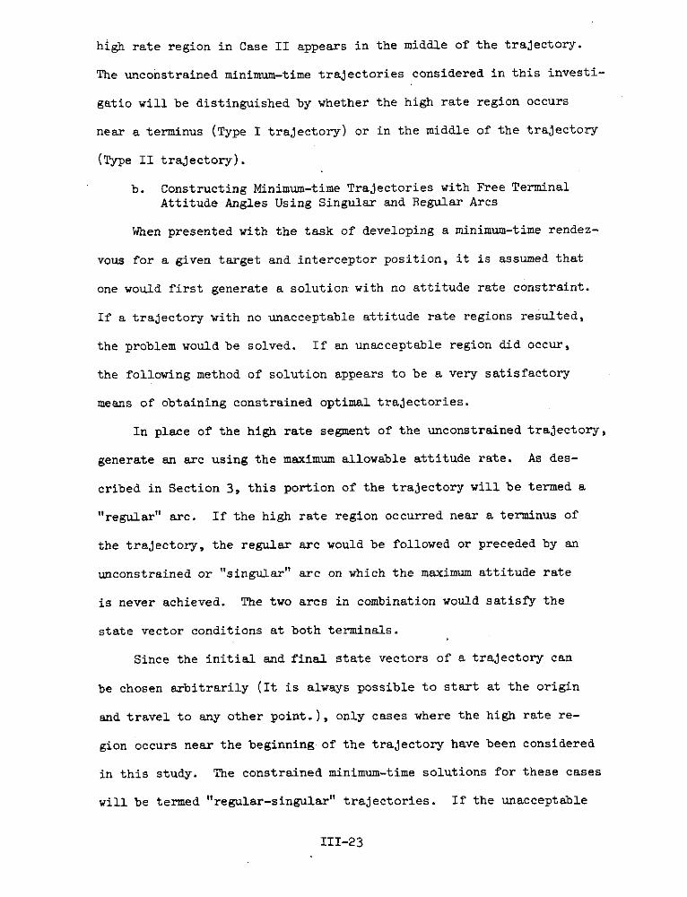
high rate region in Case II appears in the middle of the trajectory.
The unconstrained minimum-time trajectories considered in this investi-
gatio will be distinguished by whether the high rate region occurs
near a terminus (Type I trajectory) or in the middle of the trajectory
(Type II trajectory).
b. Constructing Minimum-time Trajectories with Free Terminal
Attitude Angles Using Singular and Regular Arcs
When presented with the task of developing a minimum-time rendez-
vous for a given target and interceptor position, it is assumed that
one would first generate a solution with no attitude rate constraint.
If a trajectory with no unacceptable attitude rate regions resulted,
the problem would be solved. If an unacceptable region did occur,
the following method of solution appears to be a very satisfactory
means of obtaining constrained optimal trajectories.
In place of the high rate segment of the unconstrained trajectory,
generate an arc using the maximum allowable attitude rate. As des-
cribed in Section 3, this portion of the trajectory will be termed a
"regular" arc. If the high rate region occurred near a terminus of
the trajectory, the regular are would be followed or preceded by an
unconstrained or "singular" arc on which the maximum attitude rate
is never achieved. The two arcs in combination would satisfy the
state vector conditions at both terminals.
Since the initial and final state vectors of a trajectory can
be chosen arbitrarily (It is always possible to start at the origin
and travel to any other point.), only cases where the high rate re-
gion occurs near the beginning of the trajectory have been considered
in this study. The constrained minimum-time solutions for these cases
will be termed "regular-singular" trajectories. If the unacceptable
III-23

region occurs in the middle of the trajectory, the regular arc would
be preceded and followed by singular arcs. These constrained trajec-
tories will be denoted "singular-regular-singular" trajectories.
c. Degrees of Freedom in Solving the Constrained
Minimum-time Problem
It has been pointed out above that the development of minimum-
time rendezvous trajectories without rate constraint requires the
solution of a two-point boundary-value problem with unknown para-
meters at both terminals. The solution of the constrained problem
likewise requires the determination of unknown parameters at both
ends of the trajectory. Since the state vector equations of motion
are non-linear in both the constrained and unconstrained problems,
it is necessary to integrate these equations numerically. The ad-
joint time history may be generated by using a state transition matrix
which will be discussed below. State and adjoint vector time histories
must be generated repeatedly, adjusting the free variables until the
state vector conditions (and in some cases adjoint vector conditions)
are satisfied at both terminals. The degrees of freedom in the prob-
lem are the actual number of variable quantities or parameters in the
iteration procedure.
d. Junction and Terminal Conditions
The first problem that must be surmounted in generating multiple-
arc minimum-time trajectories is the determination of the required ad-
joint conditions at junction and terminal points and the development
of means to satisfy these conditions. Consider first junction points.
Both the state vector x and the adjoint vector must be continuous
across the junction. Thus, since p5 = p = 0 on asingular arc, both5
p and p must reach zero simultaneously at the point on the regular
III-24

arc that is to be a junction point with a singular arc.
At terminal points the first four components of the expanded
state vector (two components of position and two components of
velocity) are specified. The fifth component, the angle specifying
the direction of thrust, is left free to vary. If a component of
the state vector is left free to vary, by the transversality condi-
tion (see Reference III-3) the corresponding component of the adjoint
vector must be zero. Therefore, p 5 must be zero at the terminals.
Obviously this requirement is already satisfied if a terminus is
reached while on a singular arc. Regular arcs must be adjusted so
that this condition is met.
Before proceeding with the development of the equations that
must be satisfied in order to ensure that the adjoint junction and
terminal conditions are satisfied, it is necessary to consider the
state transition matrix governing the adjoint vector. Recalling
that the true anomaly has been substituted for time as the indepen-
dent variable, the state transition matrix is
4-3cosO -3sine 6e-6sin8 6cose-6
-sine cose 2cose-2 2sine. (111-39)
0 0 1 0
2-2cos6 -2sine 36-hsine 4cose-3
Then
Pl()i pl(O)
P2 (e) 0 P2 (0)
P3(8) P3(0)(III-O)
p(e) p4(0)
111-25

e. Regular-Singular Trajectories
As stated previously regular-singular trajectories will be
substituted for unconstrained trajectories having an unacceptably
high attitude rate near the start of the trajectory. Recall that
at the start of the regular arc, i.e., at the initial point of the
trajectory, p 5 is zero since s5 is free. At the end of the regular
arc, when jumping to a singular arc, both p 5 and p5 must be zero.
The true anomaly will be defined to be zero at the initial
point of the trajectory. At this point we can say in general that
p 4( 0 ) = k p2 (0) (III-41)
P2(0) = k p1 (0) - k p3(0) (111-42)
where k and k are arbitrary constants. The motivation for the.choice
of these equations will be made clear later in this section. On a
regular arc the attitude angle varies at a constant rate so that
x5(e) = x 5(0) + ae . (111-43)
From (III-32e)
p = n(p2sin x5 - p)cos x . (111-44)
Setting the constant n to unity and using (111-43), (11-44) becomes
p; = p2sin(x 5(0)+oe) - p4cos(x 5 (0)+oe) . (111-45)
The use of the components of the adjoint vector in optimization
problems has always suffered from the fact that the values of these
parameters generally have no physical significance. For this reason
obtaining a reasonable first guess to start the iteration procedure
is usually very difficult. Without a first guess that is close to
III-26

that which gives convergence, many iteration procedures fail to con-
verge to the desired solution. In making a first guess to solve the
constrained minimum-time problem, the components of the adjoint vector
and the total flight time that gave convergence in the unconstrained
problem serve to provide reasonable values. However it was noticed
that by iterating on variables having physical significance an even
better first guess can be made, and the iteration procedure required
to specify the initial attitude angle and the length of the regular
arc can be avoided.
In the new procedure the following variables are chosen as the
iteration parameters; the length of the regular arc, er; the attitude
angle at the junction of the regular and singular arcs, x5(er); the
attitude rate at this junction x (er); and the total length of the
flight. Using these parameters the choice of a first guess was in-
itially made as follows. Take the initial attitude angle from the
unconstrained solution and increase the length of the regular arc
until the attitude angle on the regular arc will correspond to that
at the corresponding time on the unconstrained trajectory. Choose
this value as the length of the regular arc, the angle where agree-
ment occurs as x5 (r ), and the angular rate on the unconstrained
trajectory at this point as x(er ). Use the minimum time from the
unconstrained trajectory as the first guess for the minimum time.
Having chosen the values of these parameters, it becomes neces-
sary to generate the adjoint vector at the beginning of the regular
arc which will give these values at the end. Recalling p5 must be
zero at the end of the regular are we have
p; = 0 = p2sin x5 - phcos x5 (I-46)
III-27

and
tan x5 = p4/P2 (111-47)
Differentiating with respect to 0 in (11-47) gives
x sec2x5 (pp 2-p4p')/p (11-48)
Substituting the adjoint differential equations for p2 and p' yields
2 (-2P-P3)P2-(2P4-Pl)P4x'sec x = (-2p (111-49)P2
2
Solving for sec x5 using (111-47) gives
-[(2p2+P3 ) 2 +P4 (2p4-pl)] (111-50)
5 (p2+p )
Since x5 ( r ) has been chosen, k in the following equation has been
fixed.
P4 = k p2 . (111-51)
Employing the relationship of (111-42), namely,
p2(er) = kZ pl(er) - k P3 (er) (111-52)
and substituting both (11-51) and (III-52) in (III-50), we can
solve for k
= (111-53)(x (er)+2)(l+k 2
Since x'(0 ) is chosen e is fixed. Because the solution does not5r
depend on the magnitude of the adjoint vector, p3 is chosen arbitrar-
ily. At the start of the regular arc p5 = 0. If we assume for the
moment that 0 = 0 at the end of the regular arc, we can use 0 = -6
and obtain pl at the regular-singular junction. Then (III-51) and
II1-28

(111-52) are used to give p2 and p4 . The state transition matrix
for the adjoint vector is then used to find the adjoint vector at
the start of the regular arc. Details of the procedure can be found
in Reference 111-13.
There is no constraint present which prevents p2 and p4 from
simultaneously having a small magnitude. Examination of (111-50)
shows that should p 2 and p4 approach zero simultaneously, the magni-
tude of the attitude rate would become very large. In the event that
p2 and p4 should pass through zero simultaneously, it is clear from
(III-47) that x5 would rotate 180 degrees instantaneously. As pre-
viously mentioned this implies an infinite magnitude for x'.
By using (111-51) in (111-50) and solving for p2, the following
equation is obtained
P2 = (P k -P 3 )/(x5 + k2x5 + 2k2 + 2) = k - p3
The motivation for equations (111-41) and (111-42) should now be
obvious.
f. Singular-Regular-Singular Trajectories
The solution of the singular-regular-singular minimum-time prob-
lem clearly also requires an iteration procedure to solve the two-
point boundary-value problem. Again four degrees of freedom are
available for iteration. It is possible to directly select values
of the adjoint vector at the start of the regular arc and to iterate
on these values. However, the procedure required to satisfy the
regular arc terminal conditions is so complicated as to be impractical
in an iteration scheme. The parameters which have been chosen as
iteration variables have the advantage of physical significance as
well as simplicity. These parameters are: the length of the initial
III-29
singular arc, s; the attitude angle at the first singular-regular
arc junction, x 5(s); the length of the regular arc, er; and the
total duration of the trajectory.
The basic equations used in developing the procedure to satisfy
the regular arc terminal conditions and generate the initial adjoint
vector are nearly the same as those presented for the regular-singular
trajectory in the previous section. Therefore they will not be pre-
sented here, but the exact details are given in Reference 111-13.
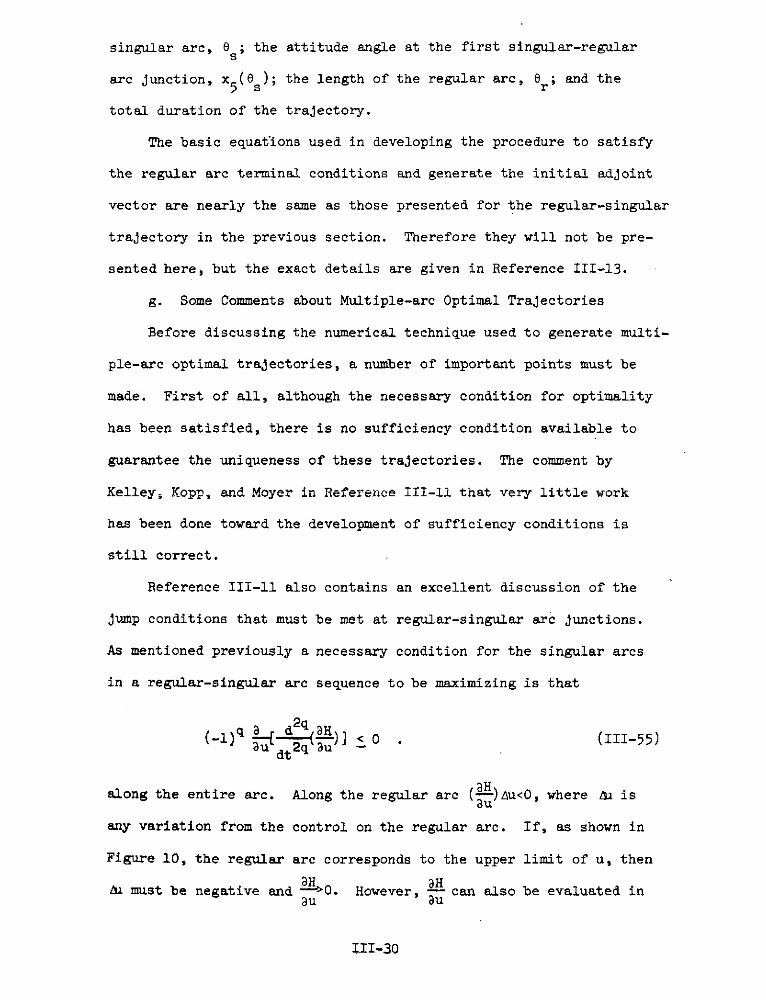
g. Some Comments about Multiple-arc Optimal Trajectories
Before discussing the numerical technique used to generate multi-
ple-arc optimal trajectories, a number of important points must be
made. First of all, although the necessary condition for optimality
has been satisfied, there is no sufficiency condition available to
guarantee the uniqueness of these trajectories. The comment by
Kelley, Kopp, and Moyer in Reference III-11 that very little work
has been done toward the development of sufficiency conditions is
still correct.
Reference III-11 also contains an excellent discussion of the
jump conditions that must be met at regular-singular arc junctions.
As mentioned previously a necessary condition for the singular arcs
in a regular-singular arc sequence to be maximizing is that
S(-1) 2q, u] <0 . (111-55)
along the entire arc. Along the regular arc (H-)Au<O, where t" isau
any variation from the control on the regular arc. If, as shown in
Figure 10, the regular arc corresponds to the upper limit of u, then
aH aHSmust be negative and 2-0. However, - can also be evaluated inau au
III-30

the neighborhood of the junction point on the regular arc by a Taylor
series expansion, leading to the conclusion that at the junction point
2qd2q- )1> 0 . (111-56)
In order to satisfy the inequalities in both (III-55) and (111-56),
q must be odd. A similar consideration of a jump discontinuity in
the control u to the lower bound produces the same conclusion.
Therefore, if a maximizing singular arc is joined to a regular arc
wtih a jump discontinuity in the control u, q must be odd.
Figure 11 depicts an example in which the singular arc joins
the regular arc when the control has become saturated and there is
aHno jump in u. In this case evaluating Lu on the regular arc gives
au
t- q u ] < 0 . (I1-57)
To satisfy (111-55) and (111-57) q must be even.
Figure 12 shows the case in which the control has become sat-
urated, but a jump to the lower control limit is desired. In this
case q must be odd.
We have previously shown that q = 1 in the minimum-time in-plane
rendezvous problem. A jump in the control must therefore occur at
the regular-singular arc junctions. This has two significant effects
in the present study. First, in the case where we are substituting
regular arcs corresponding to a particular control limit for segments
of the trajectory with unacceptably high attitude rate, we must be
able to jump to a particular control boundary. Thus the control must
either not saturate or saturate to the opposite control boundary.
Since saturation to the opposite control boundary is highly unlikely
physically, we can say in general that the jump to the regular arc
III-31

must occur prior to the onset of saturation. The second effect results
from the fact that a discontinuity in the control must occur at junc-
tions. This discontinuity is undesirable, but is much more physically
acceptable than high attitude rates.
It should finally be noted that in the solution there is no ex-
plicit control of the attitude rate on the singular.arc during the
iteration procedure. Thus it is possible for the attitude rate to ex-
ceed the limits set for the regular arcs. This problem will be dis-
cussed further in the following section.
5. Numerical Technique
A major goal of this study was the development of a dependable
iteration procedure which would solve multiple-arc two-point boundary
value problems. As mentioned in the previous chapter, the Newton-
Raphson or quasilinearization procedure was recommended by Winfield
and Johnson in Reference 111-7. This method presented a number of
difficulties in performing the iteration and had had little previous
success in solving problems with free terminal time. Therefore this
method was rejected at the outset.
It was initially decided to use the gradient technique to min-
imize the error norm. The error norm was defined as the square root
of the sum of the squares of the position and velocity components at
the final point of the trajectory, that is,
ERNORM = [X2(e )+x2 (e)+x (f )+x2(ef )]1 /2 (111-58)
The interceptor was considered to have achieved rendezvous when the
error norm became less than .001. This accuracy placed the vehicles
within approximately one hundred feet of each other. Numerical in-
tegration was performed using a fourth-order Runge-Kutta scheme over
III-32

the entire trajectory. The first four components of the adjoint vector
were updated using the state transition matrix.
The particular gradient technique employed was that suggested by
Fletcher and Powell in Reference 111-6. This method has the property
of second-order convergence, that is, the procedure converges in n
iterations when the function is a quadratic of n variables. Although
this method is recommended for use only in cases where the gradient
can be computed analytically, it was hoped that by using sufficiently
small perturbations in generating the numerical partials (PARAMETER)a (PARAMETER)satisfactory accuracy could be obtained. It should be noted that this
method has no means of distinguishing relative minima from the absolute
minimum. In the initial runs made with this method, it appeared it was
either converging fairly rapidly to a relative minimum or falling into
long narrow valleys that could not be escaped with the accuracy inherent
in the use of numerical partials. Subsequent investigations strongly in-
dicated that relative minima were being obtained.
The choice now seemed to be between changing initial guesses until
a path to an error norm which satisfied our convergence criterion was
found or altering the calculation of the error norm slightly so that
the iteration would jump off the flat place at which it had been stopped
and toward the convergence limit. The first choice was dismissed as un-
satisfactory. The second choice was briefly attempted by placing a multi-
plicative factor in front of the largest component of the error norm.
This had the effect of forcing this component to zero at the expense of
the others. At some point the multiplicative factor was removed, and the
iteration proceeded in normal fashion. This attempt was completely un-
successful.
At this stage it was noticed that, although the error norm could not
III-33

be improved at those points which appeared to be relative minima, the
behavior of the components of the error norm was reasonably linear in
their neighborhood. Therefore, when the Powell search procedure (Ref-
erence III-18) ceased to give improvement in the error norm, the follow-
ing equations were employed:
x -ax + -5 h5 + axr 6 + a--- Af = 01 ax5 5 ax 5 a e r ae - £
S35 r f
x2 2 x2 ax2x + c' + - Ax + - A +- Lf = 02 ax' ax 5 r a f
5 5 r f(III-59)
ax ax ax axx + x x + 33 Aa + 3x ref = 0
3 ax' 5 5 De r ae f
x x ax xx4 ax4 ax4 4 x+-- ' + - a +-AO +4-- A =0
6 ax' 5 ax 5 ae r fheSx 5 aer aef
Solving for the unknown changes in the parameters which will drive each
component of the error norm to zero we have in matrix form
-1ax /ax5 axl/ax 5 axl/e ax/ae -1 -xl 5
ax 2 /ax ax2/ax ax 2/aer ax 2/3a -x2 5(111-60)
ax3/ax ax3/ax 5 ax 3 er ax3 /ae f -3
axl/ax5 ax 4 "ax5 ax4/ae r ax/aef -x 4 Af
where ( ]-1 denotes the inverse of a matrix. Equation (111-60) was
easily solved using a linear simultaneous equation subroutine package
available on the IBM 360. Using the results of (111-60) repeatedly,
convergence was generally obtained within two or three steps. It was
noteworthy that the changes in the iteration parameters required to give
convergence were often quite large when compared with the perturbations
III-34

used in developing the matrix of partials and that the error norm
often increased during the process before converging.
The natural question at this point was whether the procedure
would converge starting from an initial guess rather than waiting
until the Powell method had stopped giving improvement. All types
of cases were run using only the simultaneous equation method. Un-
constrained cases were included. The results showed that the answer
to the question is generally affirmative, with the results depending
on the quality of the initial guess and on the sensitivity of the
partials in the particular trajectory involved. In those cases which
do not converge after several parameter adjustments, the Powell search
procedure can be used to improve the best guess found up to that point.
The simultaneous equation and Powell search technique are then employed
alternatively until convergence is obtained.
6. Presentation and Discussion of Numerical Results
a. Numerical Results for Four Sample Cases
A total of four cases have been selected to demonstrate the use
of trajectories with multiple optimal arcs in obtaining minimum-time
in-plane rendezvous with constrained attitude rate. Two Type 1 (high
initial rate) cases and two Type 2 (high intermediate rate) cases have
been chosen. Cases I and II are respectively trajectories of Types 1
and 2. They are typical of the trajectories with high attitude rate
which would be encountered most frequently in developing minimum-time
rendezvous trajectories. Cases III and IV are also of Types 1 and 2
respectively, but in these cases the unconstrained trajectories contain
attitude rates exceeding 1.0 x 10⁵.
The unconstrained minimum-time rendezvous trajectories for Cases
I-IV are depicted in Figure 13. Each of these trajectories was generated
III-35

using n = 3 and an integration step size of .04 radians. It should
be noted that the occurrence of high attitude rate is independent of
the starting position and the path of the time-optimal trajectory.
Only the unconstrained trajectories have been depicted since little
change in the shape of the trajectory was found when the attitude
rate was constrained.
Figures 14 and 15 present the attitude and attitude rate his-
tories for Case I. It should be noted immediately in Figure 15 that
when the attitude rate was constrained to a' = -3, the attitude rate
on the singular arc at the regular-singular arc junction exceeds the
maximum allowable magnitude. As pointed out previously, this is one
of the pitfalls that cannot be avoided when using a singular arc as
part of the total optimal trajectory. It appears that a second regular
arc segment having a' = +3 would be required in order to generate a con-
strained minimum-time trajectory which includes a singular arc and still
remains within the attitude rate limit. Rather than attempting to gen-
erate such a trajectory, it was felt that it would be more enlightening
to generate a bang-bang trajectory with l, Imax = 3. The attitude his-
tory for this trajectory is shown in Figure 14 and the time required to
rendezvous is given in Table 111.2.
The trajectories shown in Figures 14 and 15 converged very rapidly
using the results of the solution of (III-60). In no instance was a search
required and less than fifty trajectory evaluations were required in the
worst case. However, when the maximum value of c' was reduced to -2, no
convergence could be obtained. Examination of the increasing length of
the regular arc as the maximum allowable la'll is decreased seems to in-
dicate that it is simply not possible to reach the origin using a regular
arc having a' = -2.max
III-36

Table 111.2
Comparison of Minimum Rendezvous Times
for Four Sample Cases
Case I Case III
Trajectory Final Time Trajectory Final Time
Unconstrained .893519 Unconstrained .999996
a' = 10 .893529 a' = 15 1.000196max max
a'ma = 5 .893925 a'ma = 10 1.000295
max = 3 .897605 a' = 5 1.000587max max
a' = 3 .900543max
(bang-bang)
Case II Case IV
Trajectory Final Time Trajectory Final Time
Unconstrained 1.586661 Unconstrained .999357
o' = 10 1.588008 a' = 15 1.009872max max
a' = 5 1.607179 a'max = 10 1.030205
III-36a

Figures 16 and 17 provide attitude and attitude rate histories
for Case II. The trajectories shown converged very rapidly, but con-
vergence difficulties again appeared when a' was reduced to 3.max
From Figure 12 it appears that the optimal trajectory with ac' = 3max
will be singular-regular. The convergence difficulty in this case may
be due to the fact that it is difficult to iterate to a terminal sing-
ular arc of zero length.
Case III is presented in Figures 18 and 19. Because the uncon-
strained trajectory is extremely sensitive, several searches were nec-
essary to improve the guess before convergence was obtained. The con-
strained trajectories were developed without convergence difficulty,
but it is obvious in Figure 9 that the maximum allowable attitude rate
is again exceeded at the regular-singular arc junction when a' = 10max
and 5. As stated with regard to Case I, this problem can be surmounted
by using bang-bang or regular-regular-singular trajectories.
In Case IV it was again found that convergence of the unconstrained
trajectory required several searches before convergence was obtained.
The trajectories shown in Figures 20 and 21 converged rapidly, but con-
vergence was not obtained when Ia Imax was reduced to 5. It is apparent
in Figure 20 that the angle traversed on the regular arc when a' = 10max
is approximately 270 degrees. Since this angle is increasing as Ia'Imax
is reduced and since a' = -57 =ra d - 2 8 6 deg it appears that this conver-rad rad
gence failure is again indicating that it is not physically possible to
reach the origin when restricted to this attitude rate level.
A comparison of the times obtained is generating the trajectories
shown on Figures 13-21 is shown in Table 111.2. It is obvious that there
is little loss in time in using multiple optimal arcs to generate the
optimal trajectory.
III-37
b. Conclusions
The results obtained in the course of this study gave rise to
the following conclusions:
(1) Using multiple optimal arcs to generated minimum-time
trajectories when the allowable attitude rate limit
is exceeded on the unconstrained trajectory is very
feasible.
(2) Using the iteration scheme described in Section 5,
convergence to the origin occurs very rapidly in
all but the most sensitive cases.
(3) Convergence seemed to be obtainable from any reason-
able guess. If convergence is not obtained after
two or three simultaneous equation - search sequences,
a new guess may be tried. If negative arc times are
generated during the iteration, a physical difficulty
is the probable cause.
(4) As the allowable maximum attitude rate is decreased
convergence difficulties will often occur, generally
indicating that the rendezvous cannot be obtained
using that attitude rate level. In some cases con-
vergence difficulties at the lower attitude rates
may indicate that the proposed arc sequence is im-
proper. In this case a new arc sequence may be tried.
III-38

E. List of References
III-1 Apollo Navigation Working Group, "Apollo Missions and NavigationSystems Characteristics, "Technical Report 65-AW-1.O, February1965.
111-2 Bennett, F. V., and Price, T. G., "Study of Powered-DescentTrajectories for Manned Lunar Landing", NASA TN D-2426, August1964.
111-3 Citron, S. J., Elements of Optimal Control, Holt, Rinehart, andWinstron, 1969.
III-4 Clohessy, W. H. and Wiltshire, R. S., "Terminal Guidance Systemfor Satellite Rendezvous", Journal of Aero/Space Sciences, Vol27, No. 9, September 1960, pp. 653-658.
III-5 Dunn, J. C., "On the, Classification of Singular and NonsingularExtremals for the Pontryagin Maximum Principle", Journal ofMathematical Analysis and Applications, Vol. 17, 1967, pp. 1-36.
III-6 Fletcher, R. and Powell, M. J. D., "A Rapidly Convergent DescentMethod for Minimization", The Computer Journal, July 1963, pp.163-168.
111-7 Johnson, G. W. and Winfield, D. H., "On a Singular ControlProblem in Optimal Rocket Guidance", AIAA Paper 67-582, August1967.
III-8 Kaminski, P. G., Optimal Co-Altitude Rendezvous with ConstantThrust Acceleration, M.S. Thesis, Departments of Aeronauticsand Astronautics and Electrical Engineering, MassachusettsInstitute of Technology, June 1966.
III-9 Kashiwagi, Y. and Alfriend, K. T., Time-Optimal Rendezvous forElliptic Orbits, NASA CR-1036, May 1968.
III-10 Kelley, H. J. and Dunn, J. C., "An Optimal Guidance Approxima-tion for Quasi-Circular Orbital Rendezvous", Proc. 2nd Int.Congress on Automatic Control, Basle, September 1963, pp. 274-282.
III-11 Kelley, H. J., Kopp, R. E. and Moyer, H. G., "Singular Extremals",Topics in Optimization, G. Leitmann (Ed.), Academic Press, 1967.
III-12 Lewallen, J. M., "A Modified Quasilinearization Method for SolvingTrajectory Optimization Problems", AIAA Journal, Vol.5, No. 5,1967, pp. 962-965.
III-13 Miller J. J., "Minimum-Time Rendezvous with Constrained AttitudeRate", Ph.D. Thesis, Cornell University, December 1971.
III-14 Moore, R. P., "Detailed Computer Printout of Nominal Lunar ModuleDescent to the Lunar Surface", Private Communication, March 1970.
111-39

111-15 National Aeronautics and Space Administration, Lunar Flight
Handbook, Part 2 - Lunar Mission Phases, NASA SP-34, 1963.
III-16 Paiwonsky, B. H. and Woodrow, P. J. A Study of Time-Optimal
Rendezvous in Three Dimensions, AFFDL-TR-65-20, January 1965.
III-17 Pontryagin, L. S., Boltyanskii, V. G., Gamkrelidze, R. V. andMischenko, E. F., The Mathematical Theory of Optimal Processes,Interscience Publishers, 1962.
III-18 Powell, M. J. D., "An Efficient Method for Finding the Minimumof a Function of Several Variables without Calculating Derivatives",The Computer Journal, July 1964, pp. 155-162.
III-19 Robbins, H. M., "A Generalized Legendre-Clebsch Condition for theSingular Cases of Optimal Control", IBM Journal of Research and
Development, July 1967, pp. 361-372.
III-40

FIGURE 1 PROFILE OF TYPICAL APOLLO MISSION
LUNAR MODULE DESCENT FROM ORBIT
-CSM 60 N. MILE PARKING ORBIT
INITIATE HOHMANNDESCENT
- -INITIATE Lf POWERED
LANDING / DESCENT
SITE21 0
CSM POSITION AT LANDING
FIGURE 2 PROFILE OF APOLLO MISSION LUNAR MODULE TERMINAL DESCENT
TO A LANDING SITE BELOW THE MEAN LUNAR SURFACE
ALTITUDE ABOVE39862 39492 39635 36995 34000 MEAN SURFACE
(FEET)28812
16540
-10770280 240 200 160 120 80 40SURFACE RANGE (MILES)
691 659 619 571 515 451 347TIME (SEC)
III-41

FIGURE 3 THREE PHASES OF TERMINAL POWERED DESCENT
12
1 ANGLE BETWEEN THRUST VECTOR
! 35 AND LOCAL HORIZONTAL10
8- r36
ALTITUDE ABOVE
LANDING SITE
(103 FEET) 6 45
4-47
49
2 '--540 5 70 74 76 81 83 86 89
BRAKING VISIBILITY FINAL DESCENT
FIGURE 4 RLS ASCENT SEQUENCE
ORBITING BASE
WHEN RLS REACHES RLS ORBIT BEFORE
CIRCULAR ORBIT RENDEZVOUSC RENDEZVOUS
MOON
HOHMANNTRANSFER-ORBIT
S---LAUNCH POINT
ORBITING BASE
AT LAUNCH
III-42

Figure 5.
Coordinate Systems
Y
z
Target x
Vehic
It P Interceptor1 Position
Center ofattraction X
Target VehicleOrbit
nII-43

Attitude History (Type I)
a = tan-1 (u Ux)
300
200
(degrees)
100
0
0.2 0.4 0.6 0.8 1.0
e (radians)
Figure 7.
Attitude Rate History (Type I)
10
a'(rad/rad)
0 e
0.2 o.4 0.6 0.8 1.0
-10
25III-
111-44

Figure &
Attitude History (Type II)
to = tan 1 -Ux
300
200
a(degrees)
100
0 o. 4 0.8 1.2 .1.6
e (radians)
Figure 9.
Attitude Rate History (Type II)
20.
10
(rad/rad)0.4 0.8 1.2 1.6
-10
-20
III-45

Figure 10
Jump to the Upper Bound
atm
singular regulararc arc
0a' e(rad)(rad/rad)
q oddmin
Figure 11.
Saturation to the Upper Boundregular
are
max
(rad/rad) e (rad)q even
min
Figure 12.
Saturation to the Upper Bound with Jump
a'max
singular
a' e(raa)(rad/rad)
q odd
in regulararc
* These figures have been adapted from similar ones in Reference III-9.
III-46

Figure 13.
Unconstrained Minimum-time Rendezvous Trajectories for Cases I-IV
x-l0' (ft)
1.5
1.0
case II0.5
1.5 1.0 0.5 -0.5 -1.0 -1.5
Y.10 5 (t)
-. 5 case IV
-1.0
case I-1.5 case III

Figure 14.
Attitude Histories for Case I
250
a' unconstrained
------ a' = 10maxa' =5max
Smax
(deg)
150
1000.0 0.2 o. 0.6 0.8 1.0
0(rad)

Figure 15.
Attitude Rate Histories for Case I
20.
5.1\
, .2 .4I .8 1.0(rad/rad) e (rad)
I
-25-
HH -10.
-15. unconstrained----- a' = 10
max--- a' = 5
-20. - maxmax
-25.
-30.

Figure 16.
Attitude Histories for Case II
300
'n (deg)0
150
unconstrained
- -- a' =10max 5
100
50
0.0 0.2 0.. 0.6 0.8 1.0 1.2 1.4 1.6
e (rad)

Figure 17.
Attitude Rate Histories for Case II
25
20
unconstrained
15 = 10
I -- - ' = 5In max
(rad/rad) I I
5- ---
1.0 1.2
e(rad)5
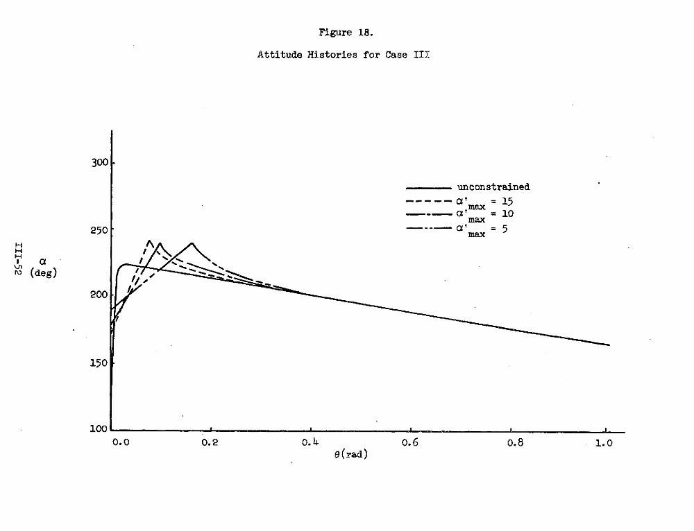
Figure 18.
Attitude Histories for Case III
300
unconstrained
----- a' = 15--- a ' = 10max
250 '----at = 5
150
1000.0 0.2 0.14 0.6 0.8 1.0
e(rad)

Figure 19.
ta i > 10 Attitude Rate Histories for Case III15 ---
I unconstrained
a x' = 15I max10 -T- --- ' = 10
max. .. . aX' = 5
max
i
at
(rad/rad)
0 I 00.2 0.4 0.6 0.8 1 9. 9(rad)0 A
I1
Ir I
-10 i
-15

Figure 20.
180 Attitude Histories for Case IV
150
120
90 unconstrained
.... ' = 156o max
60 ~- =max = o
30
0.2 0.6 0.8 1.0a a0 O e(rad)
(deg) 0.%
-30
-60
-120
-150
-18--180o----.

Figure 21.
Attitude Rate Histories for Case IV
unconstrained
a' = 15max5 a' = 10
5 -max
0. 0.4 0 6 0.8 1.0a' 0 -._-- , , .e(rad)
(rad/rad)
1 Ii I
-5 I
-10
I I
-15
j a> 105

Chapter IV: Guidance and Navigation
1. Introduction
Based upon the mission profile discussed in Chapter II, the
Guidance and Navigation (G&N) requirements for the mission can be
separated into five distinct phases:
1) descent to hover
2) terminal descent and landing
3) ascent and acquisition
4) rendezvous and docking
5) abort
Since the state-of-the-art in navigation instrumentation is constantly
changing, the following discussion will deal solely with the overall
systems design of the G&N system. A detailed component design could
only be done when the ship is designed in detail.
2. Laser Radar Ranging System
As will be shown in the chapter on communication, one reason why a
laser communication system is impractical is that the relative position
uncertainty between the LOS and LSV makes it extremely difficult to
accurately align the optics necessary for such a system. But, if we
use our microwave antenna system to gain position information about
the LSV, then we could use this data to "boresight" a set of transmitt-
ing receiving optics aboard the LOS. Since modulation of the returning
laser beam is not required in a radar system, those problems are elimi-
nated; and by using the microwave system for coarse pointing information,
the problems associated with the initial acquisition of the LSV by the
LOS are greatly reduced. Thus, a laser-corner reflector system (aboard
the LOS) could be used to accomplish the necessary G&N measurements.
IV-1

Tracking of the LSV would proceed as follows: It is assumed that the
laser is located in a fixed position aboard the LOS and that the or-
bital trajectory of the LOS is accurately known as a function of time.
Since the laser optics are mounted aboard the LOS, any movement of the
optics relative to some null position can be translated to an angular
position relative to the LOS and hence to an absolute angular position
in space. Pointing (angular) movements of the laser optics can be
thought of as corresponding to changes in the two angular coordinates
of a spherical coordinate system mounted aboard the LOS. Range data
would be calculated from the elapsed time between the transmission of
a laser pulse and the return of its echo from the corner reflector
aboard the LSV. Thus, we can accurately pinpoint the location of the
LSV in relation to the LOS and by using the known data about the
LOS trajectory we can pinpoint the LSV in space. Velocity and accelera-
tion data would be obtained from changes in the angular position and
range data. After logging sufficient tracking data, the G&N commands
necessary to achieve the desired trajectory would be generated aboard
the LOS and transferred via the microwave link the the LSV.
Laser systems to do this job are state-of-the-art and do not require
very sophisticated optics nor large amounts of prime power. This sub-
system will form a major portion of the system used to fly the LSV. A
simplified block diagram of a system to do this job is givin in Figure
IV-1.
3. G&N Requirements
3.1 Descent to Hover Phase
Since the LSV will be leaving from the LOS there should not be any
problem in setting up either the communications link or the laser ranging
IV-2

system during this phase of the mission. By assumption line of sight
contact will be maintained after the LSV separates from the LOS until
the post-burn trajectory is established; and reestablished again before
the burn-to-hover maneuver. After the LSV is at the hover point, it
will use a high resolution T.V. system to gather topographical informa-
tion on the terrain below. Since line of sight contact (and hence
communication) is not required during this portion of the mission, the
terrain imaging data will be stored aboard the LSV until conditions
are favorable for transmitting it to the LOS.
3.2 Terminal Descent and Landing Phase
After receiving the topographical data from the LSV, the flight
crew of the LOS will select the desired landing site. Once a site
selection has been made, LOS.computers will generate the flight pro-
file necessary for a safe landing. These commands will be transferred
to the LSV via the microwave data link. After receiving the command
to descend, the LSV will operate independently of the LOS (except if
an abort situation arises) until the landing is completed and this
phase of the mission terminated. From the above discussion it is
apparent that the LOS will need its own landing radar and lunar horizon
sensors to operate independently of the LOS during landing; these sub-
systems will have to be analyzed in detail at a future date.
3.3 Ascent and Acquisition Phase
This phase can be viewed from two different and distinct view-
points. The first is that the LOS and LSV are in communication prior
to and during take-off. If this is the case, the LOS will issue the
command to lift-off the lunar surface and then subsequently fly the
ship home. Since communication existed prior to and during lift-off,
IV-3

there is no reason to worry about any acquisition problems in this
case. The second situation is that the LSV was programmed to lift
off the lunar surface at a predetermined time. Assuming that the
LSV is programmed to lift-off the lunar surface and then to enter
a stable holding orbit, it becomes a matter of reestablishing the
communications channel (and hence aligning the laser radar ranging
system) before the ship can be flown home. Establishment of the
communication channel is covered in Chapter V. Once the communica-
tions channel has been reestablished, it becomes a relatively simple
matter to boresight the laser optics and go through a simple scanning
procedure to lock-in on the corner reflector aboard the LSV.
3.4 Rendezvous and Docking Phase
Many subsystems already exist to handle this phase of the mission
with some of the new laser systems being very attractive. As before,
this area will require in depth study at a later date.
3.5 Abort
An abort condition will be said to exist if there is a failure of
any subsystem aboard either the LOS or LSV which would endanger (or pre-
vent) the LSV from returning to the LOS. Broadly speaking, this could
happen for two reasons:
Type-1: component failure
Type-2: communication failure; i.e., communication between the LOS
and LSV is lost, interrupted, or not reestablished during any vital (com-
munication dependent) phase of the mission. The general philosophy gov-
erning the action(s) to be taken in the event that an abort situation
does arise is that of trying to place the LSV in a stable holding orbit
(using its own landing radar and horizon sensors) until the situation
iv-4

CORNERILASER RETURN REFLECTO
TELESCOPE BEMAM ON,- VEHICLE--- 1'm L
AmoXQIISTIO
DETECTOR p ITRACKING
ANDACQUISITION
YSTEM RANGE SIMPLIFIED DIAGRAM OF LASERDETECTOR RADAR RANGING SYSTEM
IUTH AND RANGELEVATIO I SYSTEM
TOROUERS
AZ8ELANGLE ENCODER
READOUTPOSITION
ANGLEDATA VELOCITYLE ERR DIGITAL POIIO PROCESSOR ACELERATI
ADDER
Figure IV-I

changes and/or the necessary repairs are completed. The possibilities
of a type-1 abort are too numerous to be itemized and can only be min-
imized by the design of a reliable vehicle. Type-2 aborts might arise
from either a component failure or an obstruction in the line of sight
link between the LOS and LSV, but the action to be taken in either case
is one of achieving (or maintaining) a stable orbit and of initiating
the acquisition procedure as described in Chapter V, as is necessary
to reestablish the communications channel and terminate the abort sit-
uation.
Bibliography
1. Harden, J. W., Jr., "Advanced Spaceborn Detection Tracking and
Navigation System Studies", NASA N67-30597.
2. Wyman, C. L., "Laser Systems Research at Marshall Space Flight
Center", NASA N67-30561.
3. "Improved Lunar Cargo & Personnel Delivery System", final report,
Vol III-A, 28 June 1968, Report No. 7-28-68-4, LMSC, Sunnyvale,California.
IV-5

Chapter V: Communications System: Analysis and Design
1. Introduction
As with most other space-communications systems, the LSV commu-
nications system is predicated on direct line of sight contact between
the LOS and LSV. Ideally, this line of sight contact would be main-
tained throughout the mission, but it will be sufficient to require
direct line of sight contact during the following phases of the mission:
1) from the time that the LSV leaves the LOS until the postburn
trajectory is established
2) before and during the burn-to-hover maneuver
3) before beginning terminal descent
4) after ascent from the lunar surface
5) during rendezvous and docking.
2. Mission Requirements
2.1 Maximum Communication Range
To calculate the maximum communication range we must make some
assumptions as to the orbit of the LOS. Assuming a circular moon of
radius 1738 km and that the LOS is in a nominal 100 km circular orbit
about the moon we can calculate: R = maximum communication range, using
the Pythagorean Theorem:
(2 2; 2-----~---S1(1738 + 100) - (1738)
* R 1166 km
For the purpose of the present investigation it will be sufficient to
assume that
R = 10 3 km
V-1

Table V.1
Typical (PCM.) Data Rate Requirements
Source Signal
Bandwidth, Representation Maximum Tolerable
f, Bits/Sample Bit Rate Error
Type (i.e.,baseband) n (B =2nfm =R) Rate
Scientific Data 0 to 1 kHz 9 18 kbps 10 - 2
Engineering 0 to 1 kHz 7 14 kbps 10- 2
data
Command data 50 bps 10 - 5
Teletype 75 bps 10 - 5
Speech 0 to 4 kHz 5 40 kbps 10- 3
Real-time 15 Hz to 6 48 Mbps 10 -
television 4 MHz
(500x500 -element
picture)
Picture 15 Hz to 6 120 kbps 10 -
transmission 10 kHz
(500x500 -element
picture in
12.5 sec)
V-2

2.2 Data Requirements
There are many possible signal (message) sources, each with its
own spectral requirements. Assuming the use of PCM (pulse code mod-
ulation), which will turn out to be the case, Table V.1 can be used
to estimate the maximum data rate: RB, and the acceptable bit error
rate (or probability of error, per bit): P . It turns out that duee
to navigational requirements the capability of high resolution televi-
sion transmission is needed and, hence, a choice of RB = 5 x 10 bps
is made. As shown in Section 5, it is possible to select P = 10- 3
e
and still be able to transmit command data at the rate of 50 bps with
-5P = 10 - 5 (for command data). In order to minimize quantitizatione
errors 9 bits/sample is used, in other words at most 9 binary bits is
used to quantify any piece of data. This gives a resolution of 1 part
in 29 (1 part in 512) or approximately 0.5%.
3. System Configurations
Table V.2 summarizes the basic system configurations. The rea-
sons for considering only the S-band and CO2 laser systems are summa-
rized in Ref. V-2.
Table V.2
Basic System Configurations
Wavelength
Type of System S-Band CO 2 laserX=13 cm A = 10.6
Active acceptable acceptable
--------------------------------------------------------
Passive not acceptable acceptable
V-3
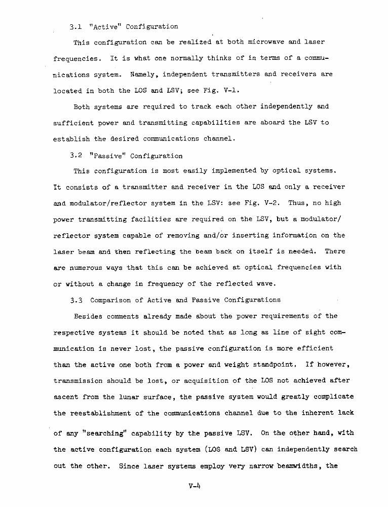
3.1 "Active" Configuration
This configuration can be realized at both microwave and laser
frequencies. It is what one normally thinks of in terms of a commu-
nications system. Namely, independent transmitters and receivers are
located in both the LOS and LSV; see Fig. V-1.
Both systems are required to track each other independently and
sufficient power and transmitting capabilities are aboard the LSV to
establish the desired communications channel.
3.2 "Passive" Configuration
This configuration is most easily implemented by optical systems.
It consists of a transmitter and receiver in the LOS and only a receiver
and modulator/reflector system in the LSV: see Fig. V-2. Thus, no high
power transmitting facilities are required on the LSV, but a modulator/
reflector system capable of removing and/or inserting information on the
laser beam and then reflecting the beam back on itself is needed. There
are numerous ways that this can be achieved at optical frequencies with
or without a change in frequency of the reflected wave.
3.3 Comparison of Active and Passive Configurations
Besides comments already made about the power requirements of the
respective systems it should be noted that as long as line of sight com-
munication is never lost, the passive configuration is more efficient
than the active one both from a power and weight standpoint. If however,
transmission should be lost, or acquisition of the LOS not achieved after
ascent from the lunar surface, the passive system would greatly complicate
the reestablishment of the communications channel due to the inherent lack
of any "searching" capability by the passive LSV. On the other hand, with
the active configuration each system (LOS and LSV) can independently search
out the other. Since laser systems employ very narrow beamwidths, the
v-4

acquisition problem is a critical one. Current state-of-the-art
laser modulators and physically realizable single section corner
reflectors require very accurate alignment of the incoming beam
for proper operation.
3.4 Choice of a System Configuration
The primary factors to be considered in the choice of a commu-
nication system configuration are: data rate, acceptable probability
of error, power requirements, acquisition and tracking requirements,
weight, volume, technical feasibility and maintenance. Taking these
factors into account, it was decided to employ an active, microwave
(S-band, A = 13 cm) configuration. This decision was based upon pre-
dicted power and weight requirements as well as the availability of
space-qualified hardware (with suitable allowances for projected
capabilities).
4. Modulation Techniques
Modulation refers to the way that information is impressed upon a
carrier waveform. There are three basic ways to do this:
1) The signal waveform is used to directly (continuously) modulate
the carrier; e.g., FM, AM.
2) The signal waveform is time sampled and these samples are used
to directly modulate the carrier; e.g., PAM, PPM, PDM.
3) The signal waveform is time sampled, quantized, and then used
to "key" a carrier; e.g., PCM/AM, PCM/FM, PCM/PM.
Type-3 modulation systems have become very popular due to the availa-
bility of low cost, low power, high speed digital electronics. State-of-
V-5

the art type-3 systems are characterized by being PCM (pulse-code-
modulation) systems; i.e., systems where the signal waveform is time
sampled and each sample is coded as a finite length binary number.
The envelope of the carrier waveform is then a string of rectangular
pulses. The various fundamental PCM systems are:
a) PCM-AM: Amplitude modulation. Data is conveyed by the
presence or absence of the carrier.
b) PCM-FM: Frequency modulation (frequency shift keying) Data(FSK)
is transmitted by transmitting a pulse of carrier at
one or two distinct frequencies.
c) PCM-PM: Phase modulation (phase shift keying or differential(PSK orPSK) phase shift keying). Data is transmitted by the phase
of the carrier (00 or 1800) for PSK; or by a change
in the phase of the carrier (from 00 to 1800 or vice
versa) for APSK.
h.1 Modulation Schemes aud Bit Error Rates
If reasonable assumptions are made about the message set and com-
munications channel, we can compute the probability of error (M bit
error rate), P , for each of the modulation schemes as a function of the
bit signal to noise ratio; E/No can be calculated. Assume that the mes-
sage set consists of {0,1} and that autocorrelation between the two
messages is -1 for PSK and 0 for FSK. As far as the channel is concerned,
assume that the a priori probability that either a 1 or 0 was sent is
identically 1/2, and that our communications channel can be modeled by an
If this is not the case, then everywhere E/N appears it should bereplaced by E(l-Y)/2N , where Y is the autocorrelation of the twomessages in question.
V-6

additive noise gaussian channel. Table V.3 gives the mathematical
expressions for P as a function of E/N that result from an analysise o
employing the above assumptions. The detailed derivations can be
found in Lawton, Refs. V-3 and V-4.
Table V.3
Pe vs. E/No for Various Modulation Schemes
Modulation Scheme P : Probability of Errore
PCM/PSK: coherent detection P = 1/2 {1 - erf E/N oe 0
PCM/APSK: differentially coherent P = 1/2 exp {-E/Nodetection
PCM/FSK: coherent detection P = 1/2 {1-erf Vr--e o
PCM/FSK: non-coherent detection P = 1/2 exp {- E/2Noe 0
These expressions for Pe are plotted in Fig. V-3 as a function of E/No .
Inspection of Table V.3 shows that:
1) The coherent or non-coherent PSK scheme offers a factor of 2
(I 3db) reduction in the required E/No (for the same Pe) when
compared to the corresponding FSK scheme.
2) The difference between PSK and APSK approaches 0 as E/N0 gets
large. For example:
P = 10- 3 > (E/No)PSK = 6.78 db, and (E/No)APSK = 7.93 db
Pe = 1 0 - 5 => (E/No)PSK = 9.58 db, and (E/No)APSK = 10.33 db
Based upon the fact that APSK systems are state-of-the art, and
the relatively small difference in the E/No required (for a given Pe)
V-7

as compared to a straight PSK system it was decided to employ APSK in
the communications system.
4.2 Synchronization
Any time division multiplex communications system such.as this
requires precise synchronization of the receiver and transmitter to
insure accurate, message decoding. The degree to which synchronization
is established directly effects the performance of the communications
system. For a PCM system, perfect synchronization is achieved when
the receiver locks in on both the frequency and phase of the transmit-
ted signal. This lock must be maintained even under very adverse
noise situations. A PCM synchronizer must have the following
properties:
1) It must be able to detect transmitted sync (synchronization)
codes even when they are severely corrupted by noise.
2) It must verify that these codes are transmitted periodically.
3) It must compute the frequency of occurrence of the sync codes.
4) It must measure the mean squared error rate to ascertain
whether or not the detected code is compatible with the
expected code.
To accomplish these four tasks, a PCM synchronizer operates in three
successive modes:
1) Search mode - here the synchronizer looks throughout the
received data for the sync pattern.
2) Check mode - having found a pattern which is suspected as
being a sync code, it tries to verify that this pattern is
indeed received periodically, thus increasing the probability
that it was in fact the transmitted sync pattern.
V-8
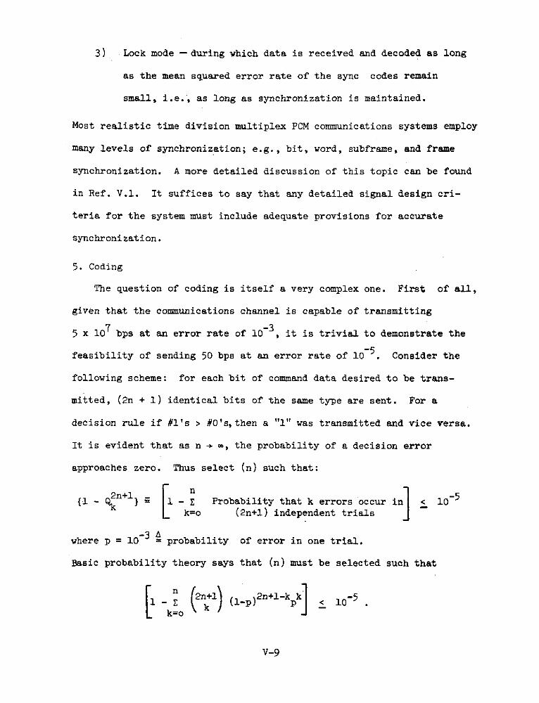
3) Lock mode - during which data is received and decoded as long
as the mean squared error rate of the sync codes remain
small, i.e., as long as synchronization is maintained.
Most realistic time division multiplex PCM communications systems employ
many levels of synchronization; e.g., bit, word, subframe, and frame
synchronization. A more detailed discussion of this topic can be found
in Ref. V.1. It suffices to say that any detailed signal design cri-
teria for the system must include adequate provisions for accurate
synchronization.
5. Coding
The question of coding is itself a very complex one. First of all,
given that the communications channel is capable of transmitting
5 x 10⁷ bps at an error rate of 10- 3 , it is trivial to demonstrate the
feasibility of sending 50 bps at an error rate of 10- 5 . Consider the
following scheme: for each bit of command data desired to be trans-
mitted, (2n + 1) identical bits of the same type are sent. For a
decision rule if #1's > #O's,then a "1" was transmitted and vice versa.
It is evident that as n -* o, the probability of a decision error
approaches zero. Thus select (n) such that:
2n+i nn{1 - n} 1 -E Probability that k errors occur in < 10-
k=o (2n+l) independent trials
where p = 10 = probability of error in one trial.
Basic probability theory says that (n) must be selected such that
Sk=o 2n+l (-)2n+l-kk] < 10-5Sv (1-p)
V-9

A simple calculation shows that:
n = 1 (2n + 1 = 3) [1 - n+] = 6 x 10⁶ < 10-5
Thus, for every single bit of command data desired to be transmitted
three identical copies should be sent to insure the desired accuracy.
Hence, 50 bps at an error rate of 10- 5 is equivalent (with simple
coding) to 150 bps at an error rate of 10-3; well within the channel
capabilities.
5.1 Data Compression
If desired, each type of data (e.g., voice, picture, scientific,
engineering and command can be coded separately and differently in an
effort to reduce the required bit rate. Thus, each individual source
coder/decoder can be designed to detect only the salient features of
the information it is processing. If this is done, the reduction in
the required bit rate could approach a factor of 10. Table V.4 shows
typical figures for the type bit rate reductions which can be expected
using data conditioning (compression) techniques. Fig. V-4 shows the
general configuration of the signal coding elements of a communication
system. The source coders are designed to handle specific types of
input data, and the channel coder is used to arrange the source messages
sequence in a form that will minimize the effects of channel noise dur-
ing transmission (note: synch coding facilities have been ignored here).
5.2 Cost Effectiveness of Coding
After the final signal specifications are set, it will be necessary
to see if a reduction of a factor of 10 in the bit rate would warrant the
increase in weight, power, and complexity of the system due to coding.
V-10
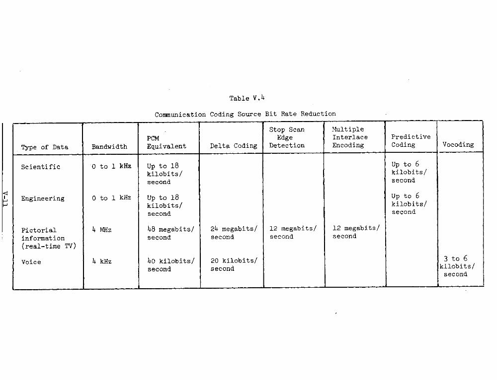
Table V.4
Communication Coding Source Bit Rate Reduction
Stop Scan MultiplePCM Edge Interlace Predictive
Type of Data Bandwidth Equivalent Delta Coding Detection Encoding Coding Vocoding
Scientific 0 to 1 kHz Up to 18 Up to 6kilobits/ kilobits/second second
Engineering 0 to 1 kHz Up to 18 Up to 6kilobits/ kilobits/
second second
Pictorial 4 MHz 48 megabits/ 24 megabits/ 12 megabits/ 12 megabits/
information second second second second
(real-time TV)
Voice 4 kHz 40 kilobits/ 20 kilobits/ 3 to 6
second second kilobits/second
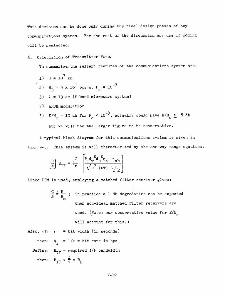
This decision can be done only during the final design phases of any
communications system. For the rest of the discussion any use of coding
will be neglected.
6. Calculation of Transmitter Power
To summarize,the salient features of the communications system are:
3-3
1) R = 103 km
2) R = 5 x 10 7 bps at P = 1 0B e
3) A = 13 cm (S-band microwave system)
h) APSK modulation
-35) E/N = 10 db for P < 10 ; actually could have E/N > 8 db
o e o --
but we will use the larger figure to be conservative.
A typical block diagram for this communications system is given in
Fig. V-5. This system is well characterized by the one-way range equation:
2 PT dT dR "aT "aRIF 16 PTdT2dR2nT]IF 16 X2 R2 (KT) LTLR
Since PCM is used, employing a matched filter receiver gives:
C E= - ; in practice a 1 db degradation can be expected
0
when non-ideal matched filter receivers are
used. (Note: our conservative value for E/N0
will account for this.)
Also, if: T = bit width (in seconds)
then: RB = l/T = bit rate in bps
Define: BIF = required I/F bandwidth
1then: BIF = R BIFV-1 B
V-12

thus, the one-way range equation becomes
R 2 R TdT2 dR2n aT T aR
Values for the system parameters, T, naT' "aR, LT LR, must be selected.
Based upon Ref. 1:
naT = 0.60 LR = 4.5 db
aR = 0.55 T 2 7 0 K
LT = 1.5 db
were chosen. Rewriting the range equation in a slightly different form:
22 16 2R2(KT)LTLR EPTdT2dR2 n B
T 2 L aT aR B
Using the above information, it is found that:
PTdT2d = 6.16 x10⁻² watts - m
Antenna diameters and transmitted power can be traded-off. However, the
final decision can be made during the actual design of the communications
system.
7. COPTRAN - Communication OPtimization Program TRANslator
7.1 Introduction
Previous sections of this chapter have dealt with the primary deci-
sions necessary to design a communications system. The approach taken
was that of a first order design, and each topic (e.g., coding, modulation
techniques, etc.) was handled as a separate entity - without regard as to
V-13

how a decision in one area might affect the choices available in
another. Of course, the reality of life is not so simple. As an
example, consider the results of the first order analysis with
PTdT2 d R2 = constant
Even here the choice of how to trade off LSV transmitting power vs.
LSV antenna size vs. LOS antenna size remains. Obviously, it is neces-
sary to develop new decision criteria to guide in this trade-off ana-
lysis. The two most pertinent ones (for space applications) are those
of designing a minimum cost system or a minimum weight system. As
will be explained in section 7.2, weight optimization is the proper
choice in the design of the LSV. Hence, to continue the first order
design, analytical (or at least functional) relationships between
PT' dT' d-, and the weight of the entire LOS/LSV communications
system must be developed. This includes such things as:transmitter
and receiver weights, antenna weights, acquisition and tracking system
weights, power supply weights, etc. It should be quite clear that even
the first order analysis no longer remains straightforward and might
not be entirely solvable without resorting to digital computers. NASA
realized this problem and in 1965 awarded a study contract (NAS 5-9637)
to Hughes Aircraft Company, Culver City, California, which in part:
... was undertaken to make a comparative analysis of micro-
wave and laser space telecommunication systems. A funda-
mental objective of the study was to provide the mission
planner and designer with reference data (weight, volume,
reliability, and costs), supplementary material, and a
trade-off methodology for selecting the system (microwave
or optical) which best suits his requirements.[Ref. V.1]
V-14

In addition to achieving the above stated goals, a FORTRAN IV computer
program called COPTRAN was developed which implemented the major results
of the study. Now, the systems design of either a weight optimized or
cost optimized communication system is reduced to inputing the proper
data to the COPTRAN program.
7.2 COPTRAN Methodology
It is necessary to investigate more deeply the ideas governing
COPTRAN. First, why the choice of either a weight or cost optimized
system, when in the final analysis a system is wanted which meets the
desired performance criteria of a minimum cost. The answer lies in the
fact that if the communications system is part of a one-shot mission
with no severe weight restrictions, then cost optimization should be used.
But, if we do have severe weight restrictions (e.g., booster limitations)
or if the system is part of a refurbishable vehicle (where AV is the
dominant costing factor), then weight optimization should be used.
Next comes the problem of implementing the chosen optimization
scheme. It can be shown (see Ref. V.1) that only four major system
parameters are needed to express the weight or cost of the entire com-
munications system. These major system parameters have the character-
istic that all the communications system parameters can be expressed in
terms of at least one of them. Of the possible sets of major system
parameters, Hughes selected the following to be the basis of their study
(and hence, COPTRAN):
1) transmitter power
2) receiver field of view
3) transmitter antenna diameter (or gain)
h) receiver antenna diameter (or gain)
V-15

The parametric weight and cost data was gathered for all the various
communications system components (with respect to the above major
system parameters). -Finally, from this data, Hughes developed monotonic,
single-valued, piecewise differentiable weight and cost "burden relation-
ships" again in terms of the major system parameters. For example, they
found that:
the weight and fabrication cost of a transmitter antenna
system are dependent upon the transmitter antenna diameter...
For small transmitter apertures, the weight is proportional
to the antenna area, and hence to the square of the aperture
diameter...For larger size apertures the weight dependence
becomes volumetric. [Ref. V-l]
(Note: The exact functional relationships described above, including
all necessary constants are given in Ref. V-1.)
Thus, what remains of the systems design of a communications channel
is to:
1) Specify the desired performance criteria (e.g., that it must
satisfy the one-way range equation for a certain set of fixed parameters)
and then,
2) optimize the remaining major system parameters using the
aforementioned "burden relationships" subject to either weight or cost
optimization, in such a way that both the desired performance criteria
and any design limits (e.g., maximum available transmitter power or
maximum available antenna diameter) are met.
Since for any realistic system it would be impossible to do this by hand
(especially if a general parametric study was desired), COPTRAN was
developed.
v-16

7.3 COPTRAN As Applied to the Design of the LSV-LOS CommunicationsChannel.
Through the generous help given us by NASA-GSFC, and in particular
Messrs. S. Schneider and R. Wigand, a copy of COPTRAN was provided.
Weight optimization was chosen since the LSV is a refurbishable vehicle,
and the input data to the program is exactly that used in the first
order analysis previously presented. A summary of the major COPTRAN
results are given in Table V.5 and Fig. V-6. Examination of these
results show that:
For RB (E/N ) = 5 x 10⁸
which was the nominal design point of the first order analysis,
PTd 2R2 = 2.5 x 10⁻¹ watts -m
which is an excellent agreement (differs by a factor of --4) with the
first order design. Since the COPTRAN results are known to be more
accurate, as well as more inclusive, they can be used with confidence to
predict the performance of the communications system and also to obtain
baseline data necessary for the design of other segments of the LSV
(e.g., the on-board power systems and the structural loading scheme).
8. Acquisition and Tracking
8.1 Acquisition
"Acquisition" is the process of aligning the antennas of the LOS
and LSV so that data transmission is possible. A simple way of doing
this employs a (radio) beacon aboard the LSV. A block diagram of the
system is shown in Fig. V-1. The basic operation consists of the LSV
transmitting a beacon signal and the LOS searching pre-determined
V-17

Table V.5
Summary of COPTRAN Results for the Nominal
Design. Point of RB-(E/No )= 5 x 10⁸
Parameter OptimumValue
dT = dR (cm) 57.6
PT (Watts) 2.25
(1) PA (Watts) 24.2 (*)
(2) PB (Watts) 15.2 (*)
(3) WA (#) 24.4 (*)
(4) WB (#) 19.0 (*)
(5) Projected Cost ($) 5 x 10⁵ (*)
(1) PA = total (LSV) transmitter input power requirement from all
sources (e.g., acquisition and tracking equipment, modulator, etc.)
(2) PB = total (LOS) receiver input power requirement; from all sources.
(3) WA = total (LSV) transmitter weight including all subsystems and
power supply.
(4) WB = total (LOS) receiver weight including all subsystems and power
supply.
(5) Includes costs for all subsystems and power supply of both the
transmitter and receiver.
(*) All values presented in this table are based on current (1970) state-
of-the-art burden relationships and might be expected to decrease slightly
(10-15%) by the proposed date of the mission.
V-18

sectors of space for that signal. To do this, the LOS would employ a
sensitive programmable scanning receiver with a steerable, variable
field of view antenna. At the start of the acquisition sequence, the
LOS would scan with a very broad (large) field of view antenna charac-
teristic till it found the beacon signal. Then, the antenna pattern
would be narrowed, and the scan procedure reexecuted. Thus, by alter-
nately scanning and narrowing its antenna characteristic, the LOS would
eventually lock-in on the beacon signal being transmitted by the LSV.
Next, the LOS would transmit alignment commands to the command receiver
aboard the LSV. These commands serve to orient the LSV in the proper
attitude for (re-)establishment of the communications channel. After
achieving the proper orientation, control would be transferred to the
normal communications system, pending confirmation from the LOS that
the channel was indeed operating. If for some reason the channel was
not established or was inadvertently lost, control of the LSV would
revert to the command receiver, and the acquisition sequence would
begin again.
8.2 Tracking
"Tracking" is the term used to identify that procedure by which,
after acquisition is achieved, the antennas of the LSV and LOS are kept
in the proper orientation for communication to occur. The LOS and LSV
will have separate tracking subsystems, each consisting of coupled
mechanical and electronic servo systems. Coarse mechanical positioning
would be done by a mechanical positioner with the fine adjustments
being accomplished electronically (through proper antenna phasing).
V-19

The ideas governing such a system are as follows: with communication
taking place, the effective orientation of the receiving antennas will
constantly be perturbed ever so slightly in an effort to locate the
direction that would maximize the mean squared received signal power.
This information (coupled with any prior knowledge of the trajectory
of the signal source) would then be used to electronically steer the
transmitting antennas. This form of "electronic steering" works well,
but only for small deviations from the true mechanical orientation of
the antenna. Hence, once the difference between the true position of
the transmitting antenna and its "electronic position" exceeds some
prescribed limit, the mechanical positioner would be called upon to
reorientate the antenna in such a way as to null out that difference.
Following this, control would revert to "electronic steering" begin-
ning the tracking sequence all over again.
V-20

SYSTEM NOMENCLATURE
Symbol Description
BIF equivalent noise bandwidth of the IF stage. The
maximum RB = BIF.
[jjIF or IF total receiver signal-to-noise power within BIF'
With a matched filter receiver S/NIF = (E/No ).
E- predetection signal energy in each bit/noise power0
spectral density
dT transmitter antenna diameter
dR receiver antenna diameter
K Boltzman's constant, 1.38047 x 10²³ Joules/degree Kelvin
1/LT transmitter line losses
1/LR receiver line losses
N thermal noise power in the IF bandwidth, N = N Bo IF
N equals KT
NR resultant noise in the analog output signal of a PCM
System caused by both quantization and bit error noises
Pe probability of a bit detection error
PT transmitter power output at the transmitter output terminals
R communication range
RB downlink bit rate
S signal energy
T total effective system noise temperature referred to the
preamplifier input
naT transmitter aperture efficiency
V-21
raR receiver aperture efficiency
T transmitted bit width = 1/RB
X transmitter carrier wavelength
MODULATION NOMENCLATURE
Analog Systems
AM amplitude modulation
FM frequency modulation
Uncoded Pulse Systems
PAM pulse amplitude modulation
PPM pulse position modulation
PDM pulse duration modulation
Coded (Digital) Pulse Systems
PCM pulse code modulation
V-22

REFERENCES
V-1. "Parametric Analysis of Microwave & Laser Systems for Communicationand Tracking", Hughes Aircraft Company, Culver City, California,work done under NASA Contract No. NAS 5-9637:
Volume I ; October 1970; NASA CR-1686Volume II ; February 1971; NASA CR-1687Volume III; February 1971; NASA CR-1688Volume IV ; February 1971; NASA CR-1689
V-2. Blake, A. M., "Lunar Shuttle Vehicle Communications Systems,August 1970 (Internal Interim Report).
V-3. Lawton, J., "A Comparison of Binary Data Transmission Systems", Pro-
ceedings of the 2nd Annual Conference on Military Electronics, IRE,
1958.
V-4. Becker, H. and Lawton, J., "Theoretical Comparison of Binary DataTransmission Systems", Cornell Aeronautical Laboratory, ReportCA-1172-5-1, May 1958.
BIBLIOGRAPHY
1. Kalil, F., "Optical and Microwave Communications -A Comparison",NASA TN-D-3984, May 1968.
2. Anon., "Parametric Analysis of Microwave & Laser Systems for Com-munication and Tracking - A Summary", NASA TR-R-309, April 1969.
3. Wyman, C. L., "Laser Systems Research at Marshall Space FlightCenter", NASA N-67-30561.
4. McElroy, J. H., "Carbon Dioxide Laser Systems for Space Communica-tions", presented at ICC 1970, San Francisco, California.
5. Lawton, J., "Investigation of Digital Data Communication Systems",Cornell Aeronautical Laboratory, January 1961, UA-1420-S-1; Phase-1Report.
6. Lawton, J., "Investigation of Analog and Digital Communications Systems",Cornell Aeronautical Laboratory, May 1963, UA-1420-S-3; Phase-3, finalreport.
7. Harden, J. W.,Jr., "Advanced Spaceborn Detection, Tracking and Navi-gation System Studies", NASA N-67-30597.
8. Stokes, L. S., Brinkman, K. L., Pratt, W. K., Weber, J. W., "User'sManual for COPTRAN II; A Method of Optimum Communications SystemDesign", NASA Electronic Research Center, Cambridge, Mass., Report No.P68-267. Work done under contract # NAS-12-566.
V-23

LOS LSV
RCVR RCVR
T/RT/R aw SWITCH
SWITCH1ANTENNA ANTENNA
XMITTER XMITTER
"ACTIVE" CONFIGURATION
Figure V-I
LOS LSV
RCVR RCVR
MODULATOR
SWITCH
OPTICS REFLECTINGMIRROR
XM ITTER
"PASSIVE" CONFIGURATION
Figure V-2
V-24

-I
10
NON - COHERENT
-2 FSK
-3
10
10
10-4
Figure V-3
-8 -4 0 4 8 12E/No (in db.) V-25

SOURCE BIT RATE REDUCTION
SOURCE DESTINATIONCODERS DECODERS
PICTORIAL PICTORIALDATA DATA
CONDITIONING RECONSTRUCTION
CHANNEL TO CHANNELCODER DEMODULATOR DECODER
SPEECH FORMAT MOOU OR SPEECH TOSOURCES DATA ) ODATASOURCES 0 DATA CODING DECODING DATA DESTINATION
CONDITIONING RECONSTRUCTION
o
SCIENTIFIC AND SCIENTIFIC AND
ENGINEERING ENGINEERING
DATA DATACONDITIONING RECONSTRUCTION
a. TRANSMITTING SYSTEM b RECEIVING SYSTEM
Figure V-4

FUNDAMENTAL DIGITAL COMMUNICATIONS SYSTEM BLOCK DIAGRAM
7 PREAMP.
DIGITAL Ic+ fDOPPLER +
SIGNAL SIDEBANDS
FIRST DETECTOR,
ANALOG TO MODULATOR MXERANALOG TO
DIGITAL CONVERTER fc i-F MATCHEDSIGNAL INCLUDES SAMPLER MODULATOR fm POWER + R-FMATCHED P.SOURCE AND CODER, i.e. DRIVER AMPLIFIER SIDEBANDS AMPLIFIERMPLIFIE FILTER
fm PCM ENCODER
DRIVING CARRIER + SIDEBANDS2nfm SIGNAL SIDEBANDS 8,F
=2nfm
DC FREQUENCY-J-OSCILLATOR VOLTAGE CONTROLLING DISCRMINATOR LOW-PASS
CONTROLLED VOLTGE FOLLOWED by I FILTER
.4=~ ~OSCILLATOR VOLTAGE LOW fmSLOW-PASS FILTER
Figure V-5

6 90
5 z 80
zr) -70
4- E_ D -60
--- -
0
2 50
PT 40
l R30107 8 0 9 100
OIO 4O lo
Re ( E/N o)
Figure V-6

Chapter VI: Propulsion Systems
This chapter summarizes the reasons for the selection of a liquid
oxygen - liquid hydrogen (L02/LH2 ), pump-fed Bell rocket engine for the
lunar shuttle vehicle (LSV). The chapter also develops an analytical
model which can be used to predict pressure and flow transients in a
gaseous oxygen-hydrogen (GO2/GH2 ) reaction control rocket engine feed
system.
1. Main Propulsion System
The candidate propellants can be grouped as cryogens, i.e., L02 /LH2
or LF2/LH2, or space storables, i.e., FLOX/CH4 . The cryogens using liquid
hydrogen as fuel, are characterized by low bulk density, high specific
impulse, and non-overlapping liquidus range. FLOX/CH 4 exhibits a moderate
high specific impulse and high bulk density.
Earth storables were not considered because of the low specific impulse
and storage problem associated with maintaining earth ambient temperatures
in order to keep the propellant from freezing.
Table VI.1 lists the propellant combinations considered and the propel-
lant weight penalties (+) or savings (-) incurred, when compared to LO 2/LH2
with a specific impulse (Isp) of 451 seconds. The calculations for the
propellant weight penalty assumed LEM (Lunar Excursion Module) ascent and
descent velocity data with a vehicle (w/o propellant) and payload weight of
6,011 pounds and propellant weight of 14,238 pounds.
The weight summary indicates that LF2 /LH2 yields a slightly lower pro-
pellant weight. LF2/LH2 was ruled out because of the highly toxic and
reactive character of florine and it was felt that the slight weight saving
over L02/LH2, did not warrant development of a reliable and space proven
VI-1

Table VI.1
Propellant Isp Mixture Ratio % Difference
Combination (seconds) O/F From Baseline
FLOX/CH4 400 5.25 + 20.3
FLOX/CH4 410 5.75 + 15.7
LO2/LH2 440 6 + 3.8
LO2/LH2 451 6
LF2/LH2 468 13 - 5.35
engine using LF2/LH2. Successful launches of the Centaur and Saturn
vehicles have demonstrated the reliability of pump-fed rocket engine
systems with LO2/LH2 as the propellants. The choice of L02/LH 2 over
FLOA/ 4 was based on weight saving.
Table VI.2 indicates the propellant combinations along with the
various rocket engines which were considered in the selection of the
main propulsion system. The LO2/LH2 pump-fed Bell engine was selected
for the LSV. A pump-fed system was selected over a pressure-fed system
due to the weight savings in propellant storage equipment and improved
performance for the Bell engine.
The tank pressurization which is required to provide net positive
suction head for full thrust pump-fed engine operation can be obtained
by bleeding warmed propellant from the regenerately cooled engine during
an idle phase. The engine pump can operate on the propellant head availa-
ble from the propellant setting without external pressurization of the
tanks at idle. Thus, the requirement for leakproof storage and control of
a high pressure tank pressurization gas such as helium is eliminated.
VI-2

Table VI.2
Engine Data
Propellant Feed Mixture Chamber Isp Expansion Engine Engine Thrust Throttle
Combination Ratio Pressure Delivered Ratio dia/length Weight RatedO/F (psia) (seconds) (c) in/in lbs.
Pump 6 900 451 100LO/2 LH2 Pressure 6 00 5 25/53 152 8,000 8:1
2 2 Pressure 6 100 445 100
Pump 13 900 468 1001. LF /LH 25/54 152 8,000 8:11. F2 /LH2 Pressure 13 100 442 100 25/54 152 8,000 8:1
Pump 5.75 600 410 100FLOX/CH4 Pressure 5.75 100 387 100 31/61 152 8,000 8:1
2. 02/H2 Pump 5 440(nom) 57:1 39.67/ 290 15,000 Nou> 439(min) 70.23
3. 02/H2 Pump 5 444(nom) 60:1 39.67/ 315 15,000 10:1439(min) 70.23
Pump 5.25 500 3994. FLOX/CH Pump 5.25 800 399 60:1 41/21 89 5,000 10:1
All engines are regeneratively cooled.
1. Bell Engines 3. RL10A-3-7
2. RL10A-3-3 4. Rocketdyne

The gaseous propellant boiloff can be used for the bi-propellant
reaction control system (RCS) supplemented with an auxiliary means to
transform the liquid propellant to the gaseous phase.
The Bell engine uses regenerative cooling of the main combustion
chamber and radiation cooling of the exhaust nozzle, where the heat flux
level permits. The additional pressure required to force the fuel cool-
ant through the coolant passages can be supplied by a turbopump.
An expander cycle, i.e., the turbopump driving gas is returned to
the main chamber for combustion and expansion at full engine area ratio,
was selected over an open cycle, i.e., turbopump driving gas is dis-
charged overboard at less than main chamber expansion ratio, due to the
inherent capability of the former to provide a higher specific impulse
performance.
2. Reaction Control System
The RCS provides impulse for small vehicle velocity changes, atti-
tude maneuvers, and attitude or station keeping. The RCS rockets will be
of the bi-propellant type utilizing GO2/GH2 . The use of a common oxidizer
and fuel for both main and reaction control propulsion simplifies the fuel
handling along with utilizing boiloff from the main propellant tanks.
An auxiliary means of providing gaseous propellants from liquid propellants
should be provided by means of a heat source in smaller auxiliary propel-
lant tanks.
The location and number of rocket nozzles required to yield suffi-
cient redundancy was found to be a 12-nozzle configuration shown on page
VI-5.
VI-4

3
1 1
12 NOZZLES
In order to aid in the design of the gaseous bi-propellant RCS an
analytical model was developed to predict the pressure and flow transients
in the proposed GO2/GH2 reaction control rocket engine feed system. The
one dimensional equations of momentum and continuity are reduced by the
method of characteristics from partial derivatives to a set of total
derivatives which describe the state properties along the feedline.
System components, e.g., valves, manifolds, and injectors are represented
by pseudo steady-state relations at discrete junctions in the system.
Solutions were effected by a FORTRAN IV program on an IBM 360/65. The
results allow evaluation of the relative effect -of manifold volume, com-
bustion lag time, feedline pressure fluctuations, propellant temperature,
and feedline length on the chamber pressure transient for a 100 pound
thrust-rocket engine. The analytical combustion model is verified by
good correlation between predicted and observed chamber pressure transients.
The developed model enables a rocket designer to vary the design para-
meters analytically to obtain stable combustion for a particular mode of
operation which is prescribed by mission objectives.
VI-5

3. General
In the area of spacecraft propulsion devices, reaction control
system (RCS) rocketry is unique. The RCS rocket maneuvers and steers a
spacecraft in the absence of aerodynamic forces. These engines operate
in the pulse mode for a major portion of the time; as a consequence,
their design requirements differ substantially from those of larger
devices. The following are the significant design requirements: high
thrust to minimum impulse ratio, fast response time, and a long cycle
life. The present RCS used in manned spaceflight is a liquid bipropel-
lant system. The system basically consists of pressurized propellant
tanks, propellant lines, and the rocket engine assembly, which is com-
posed of propellant valves, injectors, and a thrust chamber.
The pulsed operation of the present RCS engine and its feed system
are responsible for hydraulic transients capable of severely altering
engine performance. Rapid operation of the propellant valves generates
elastic waves in the propellant lines. The elastic waves generated in
the oxidizer and fuel have different propagation velocities and as a
result cause the oxidizer-fuel ratio in the engine to vary. The flow in
the manifolds and internal passages of the injector is coupled to the
thermochemical processes in the combustion chamber as well as to the
oscillating feed system flow. The manner in which this coupling contri-
butes to the observed combustion instability is unknown, but certainly
significant.
4. Previous Work
The dynamic characteristics of large liquid-propellant rocket
engine feed systems has been the subject of many analyses during the
vI-6

past two decades. The low-frequency instability analytical model
currently used to predict stability limits has evolved from the contri-
butions of many researchers [VI-1, -2]. Crocco et al [VI-3] showed that
small combustion delays are instrumental in initiating high-frequency
combustion instability. Such delays are probably in the gas phase,
because gas mixing is the rate limiting step in the combustion process.
As a result, several researchers [VI-4,-5] have proposed various gas
mixing models, but only the model proposed by Szuch has been experiment-
ally confirmed.
Previous methods for computing feedline dynamics are applicable
only to liquid propellant rockets. Most of the rocket response studies
in the literature incorporate the lumped-element approach VI-6,-4].
With this method the major drawback is the distortion in the time-spatial
relationship between components. The most recent and promising approach,
Eschweiler and Wallace [VI-71, uses the method of characteristics to
transform the one dimensional equations of continuity and momentum from
partial derivatives to a set of total derivatives describing state prop-
erties along specified paths. System components, e.g., valves, tanks,
injectors, are represented by pseudo-steady state relations at discrete
junctions in the system.
The present study extends the characteristic method of analysis to
develop an analytic model of a gaseous hydrogen-oxygen RCS engine. The
model is capable of predicting the dynamic response of the system and
the individual components when the fuel and oxidizer valves are acti-
vated by a command signal. The unique aspects of this model are its
VI-7

capability of predicting non-steady compressible flow through feedlines
and engine components and incorporation of ignition lag, and variable
combustion lag times.
5. Analysis
5.1 Feedline Model
The one dimensional unsteady Euler equation of motion and the
equation of continuity are used to describe the flow of gas through a
pipe.
_u au 1 aP-u + u + - 0 (VI-1)at ax p ax
+ P u 2_- 0 (VI-2)at ax ax
It is assumed .that the pipe flow is free of compression shocks, i.e.,
p = p(P), and also external forces, friction, and heat conduction are
neglected.
The theory of characteristics is used to obtain the compatibility
relations, which describe the properties of the flow along a character-
istic. The compatibility relations are
D 2Sa + u = 0 (VI-3)
D ( a - u = 0 (vi-4)Dt Y-1
The characteristic slopes corresponding to Equations (VI-3) and (VI-4)
are dxdt = u + a (in direction of flow) (VI-5)
dxdt = u - a (against direction of flow) (VI-6)
VI-8

The complete derivation of equations (VI-3), (VI-h), and (VI-6) is
presented by Sidransky and Smith [VI-8]. Also, one notes that, for
isentropic flow, the compatibility equations yield the classical
Riemann invariants. Equations (VI-3) through (VI-6) can be non-
dimensionalized by specifying a reference velocity, ar, and a specific
reference length, x r. The reference time becomes tr = x /a . Equations
(VI-3) and (VI-h) are simplified by setting the Riemann invariants
equal to p and Q, respectively.
) = y2 A + U (VI-7)
Q = A - U (VI-8)Y-1
and the characteristic slopes become
dx'dt = U + A (vI-9)
dx'= U -A (VI-10)dt'
where: x' = x/xr, t' = tr/t, A = a/ar, and U = u/ar
The numerical scheme described by Markowsky [VI-9] may be used to
obtain the properties of the flow along the length of pipe. Boundary
conditions are either specified by a valve, orifice, or the junction of
the feedline and propellant supply tank. The latter junction is con-
sidered to be a nozzle intake surface and described by
A T2 A+ y- U2 (VI-ll)T 2
5.2 Valve and Injector Model
A propellant valve will be considered as a variable resistance
orifice and an injector as a multiple orifice which can be modeled as a
VI-9

single orifice with an equivalent flow area. The flow will be considered
quasi-steady, frictionless, and adiabatic. The governing equations are the
continuity
A = p As u = p At ut (VI-12)
and the quasi-steady energy equation
2 2u t
JE + = JE + - (VI-13)u 2g t 2g
Combining Equations (VI-12) and (VI-13) with the thermodynamic
relations for a perfect gas, one obtains the equation for the mass flow
through an orifice.n-l 1/2
d 0 n-l u P u
n 2 / n 1- (Pd/P) n
d o u Pu 1 - (Ad/Au)2(Pd Pu)2/ndu d u
(VI-14)
In the preceding equation, the downstream pressure and temperature
were substituted for the throat pressure and temperature and corrected
by an empirical factor "C ". Once m is calculated, the upstream and
downstream velocities are readily obtained from Equation (VI-12). Hence,
ud = /pd A , u = m/p A (VI-15)
The valve and/or injector may now be treated as a resistance
junction once the resistance, i.e., 1/Ao Cd is specified. The simula-
tion of these resistance components is considered to occur at discrete
locations along the length of the feed system, as shown in Figure VI-1.
In this study a valve is simulated as a time dependent variable
resistance orifice. Once an instantaneous value of resistance has been
VI-10

determined, the valve conditions may be computed from Equation (VI-14)
and the corresponding compatibility condition. It is the specification
of the valve resistance which forms the simulation feature of this com-
ponent. Details of simulating valves in this manner are set forth in
Ref. [VI-7]. An injector is treated as a fixed resistance component with
a variable back pressure. As such, one pressure is obtained from the
manifold conditions and the second pressure is obtained from the com-
bustor model. Features also included which extend the versatility and
usefulness of the model are hot gas ingestion through the injectors and
hot gas ingestion into the manifolds.
5.3 Manifold Model
The manifold model considers the gas to be homogeneous, quasi-steady
and assumes the gas mass, m , in the manifold at any time is given by the
perfect gas law,
VMm = P V = mm p (VI-16)m m m RT mom
The rate of change of manifold pressure may be obtained by differ-
entiating Equation (VI-16) with respect to time and setting the result
equal to the mass flow in (o ) minus the mass flow out (A.i)
dm MV aP MV aT VP aMm mm mm p m mm _ =m -m
dt R T at 2 m at R T t o iom RT omom
(vI-17)
VI-ll

solving for 3P /at gives
aP RT P aT P amm_ om m m m m (vI8)tV-(mo - m. ) + T t M t (VI-18)
at MV o 1 T at M atmm m m
In order to obtain the rate of change of manifold gas temperature
and molecular weight, one must perform an energy and.mass balance
respectively, on the manifold. The manifold pressure at time "t" can be
found by setting aPm/at = [P (t) - P m(t - At)]/At and solving for P (t).
The energy balance yields
c (t-At) m (t-At) c (t-At) m (At)
m c (t) M (t) (t-t)m vm (t) m (t)o(t-t)vm m vm m
c (t-At) ml (At)
- (t) T (t-At ) (VI-19)vm m
where
m(At) = [m(t) + m(t-At)] At/2.
Therefore T m/at can be approximated by [T (t) - T (t-At)]/At and M m/at
can be found in a similar manner by using a mass balance to find M (t).m
For hot gas ingestion into the manifold the sign of m i in Equation
(VI-18) becomes positive and in Equation (VI-19) the last term on the
right hand side becomes
c (t-At) m.(At)
c (t) m (t) Tc(t)vm m
VI-12

5.4 Combustion Model
In formulating a combustion model, the flow of propellants through
a chamber may be simplified by assuming that addition of thermal energy
takes place at constant pressure. This is a good assumption, if the
thrust chamber Mach number is less than 0.2. The process is adiabatic
because no heat is transferred to the walls. However, the process is
not isentropic, because energy has to be expended on accelerating the
gases and this energy becomes unavailable. Further simplifying assump-
tions are:
(1) The pressure at the injector face corresponds to the pressure
one computing interval earlier P (t-At).
(2) The gas mass in the combustion chamber is homogeneous.
(3) The pseudo-steady state approximates the transient for each
computing time interval At, (At < 0.000003 seconds).
(4) The propellant gas generation rate is determined from the
injection rate with a variable time delay, r, due to mixing
and chemical reaction.
(5) The physical dimensions of the combustion chamber are constant
with time, that is, chamber ablation, or nozzle throat erosion
is negligible over the time period of interest.
The analytic combustion model, with the above assumptions, is based
on a mass and energy balance of the entering propellants through the in-
jector, the hot gas exiting the nozzle, and the residual gas left in the
chamber. The mass balance on the combustor yields
mc (t) = mc(t-At) + m. (At) + mif (At) + mioi. (At) + mifi (At) - m (At)
(VI-20)
VI-13

where
m (t-At) = m (t-At) + mcf(t-At) + m (t-At)
and again
m(At) = [m(t) + m(t-At)] At/2.
The mixture ratio of the incoming propellants is obtained by divid-
ing the increments of oxidizer by the increments of fuel entering in time
interval At.
m. (At)
mMR f(At)
A more meaningful mixture ratio, i.e., one considering the time due to
mixing in a homogeneous reactor, is the accumulated mass mixture ratio,
which is
MR(t) = ([m o(t-At) + m. (At) + m .ni(At) - m n(At)] MR(t-At)
+ mco(t-At) + mio (At))/mcf(t-At) + mif(At)
+ mni(At) - mn (At) + [mcf(t-At) + mif(At)] MR(t-At) (VI-21)
The accumulated mass mixture ratio is made up of the entering propellants
and the residual mass in the combustor.
The combustor gas temperature is obtained by considering an energy
balance on the combustion chamber and neglecting the lower order kinetic
and potential energy terms. Hence,
mn (t-At)Tc(t) = m(t-At) C vc(t-At) - n cpc (t-At)] T (t - At)
+ [mio(At) + mif(At)] Cp (T+t) T CT(T+t)
+ [mio. (At) + mioi(. At)] pio (At) T io(At)
+ [mif(At) + mifi(At) ] Cpi(At) T. if(At / [m(t) c(t) + n Cpc(t)]
(VI-22)
VI-14

The combustion gas temperature is determined by applying the characteristic
exhaust velocity efficiency to the theoretical value, therefore
2 (VI-23)CT TCTT n c*
where
combustion lab injection
and
TCT = the combustion temperature of mass [mio(At) + mif(At)] at time (r+t).
The gas properties, i.e., M ,c p, and y, are obtained from combustion
performance data, which are functions of the mixture ratio. This is done
because equilibrium and frozen combustion performance of hydrogen-oxygen
is available in the form of ratio of specific heat (y), specific heat at
constant pressure (c ), combustion temperature (TCTT), and molecular
weight (M) as a function of mixture ratio and pressure. The equilibrium
and frozen combustion performance of hydrogen-oxygen used was that pre-
sented by Gordon and McBride [VI-10], corrected for gaseous propellant
combustion.
With Tc(t), Mc(t) and mc(t) known, the chamber pressure may be cal-
culated from the ideal gas law, hence,
P (t) = m (t) RoTc(t)/[VcMc(t)] (VI-24
The mass flow through the nozzle is given by the standard nozzle
relations:
for choked flow,
mn(t) = Ant Cdn Pc(t) LRct MT(t) 1 2 c2 + 2[c) - 1
(VI-25)
VI-15

and for nonchoked flow,
(vI-26)
With the above combustion model, calculations of the chamber pressure
and temperature of the residual gases requires an iterative solution. The
solution is accomplished by selecting the efflux mass, n (t), through the
nozzle and if the computed value of m n(t) from Equation (VI-25) or (VI-26)
does not agree within a.prescribed delta, a new choice is made and the proc-
ess is repeated until convergence to a desired tolerance is achieved.
Combustion lags, i.e., due to gas mixing and chemical reactions, are
incorporated into this model by specifying a finite period of time between
the instant the propellant enters the chamber (time = tinjection), and
the time when it is burned (time = tinjection + tcombustion lag (T)
6. Results and Discussion
6.1 Feedline Dynamics
The feeding system and engine assembly arrangement which is investi-
gated is the fast response type. That is to say, the oxidizer and fuel
valves feed directly into the manifolds, thus eliminating any pipe fill
and emptying time lag which are inherent when the propellant valves and
manifolds are separated by a length of feedline.
Figure VI-2 illustrates the effect of feedline dynamics on manifold
pressure and mixture ratio with combustion suppressed. The valve opening
VI-16

and closing time is 5 milliseconds (ms.). This valve was used throughout
this study along with the valve resistance given by Eschweiler and Wallace
[VI-7T. The initial conditions for this and succeeding runs are given in
Table VI.3 along with the pertinent design parameters.
The variation in fuel and oxidizer manifold pressure is caused by
the pressure waves, which are initiated when the valve is opened. The
opening of the propellant valve initiates an expansion wave propagating
upstream from the valve towards the gaseous supply tank. The junction
between the supply tank and the feedline can be considered to be a nozzle
intake surface, and therefore nearly a constant pressure surface, so that
the incoming expansion wave is reflected as a compression wave. The re-
flected compression wave travels downstream and is partially swallowed
and reflected upon reaching the valve. The valve boundary is not a con-
stant pressure surface so the reflected wave maintains the same sign,
i.e., compression waves are reflected as compression waves and expansion
waves are reflected as expansion waves. So, the wave, upon reaching the
valve, is reflected as a slightly weaker wave. This phenomena is most
evident in the fuel side of the feed system due to the greater wave propa-
gation velocity which results in a higher frequency of pressure oscilla-
tion. The result of the out of phase oscillation in the two feedlines is
to produce a variable mixture ratio shown in Figure VI-2. From the pre-
ceding observations and discussion, one can conclude that the feedline
dynamics are capable of producing alterations in the mixture ratio, i.e.,
accumulated mass mixture ratio, and consequently in engine performance.
VI-17

Table VI.3
Summary of' System Parameters
RUN PT TT LO LF d D D Pc L* V A Dnt c(psia) (OR) (in.) (in.) (in.) (in.) (in.) (psia) (in.) (in.3) (in. 2) (in.)
250 - 257 125 200 60 60 .5 .292 .378 80 25 17.8 3.56 .952 .95
450 - 457 125 400 60 60 .5 .339 .433 80 25 17.8 3.56 .952 .95
471 125 " 60 6" " " " " " "
472 125 " 30 30 " " " " " "
473 125 " 30 60 " " " " " " " " "
500 150 500 60 60 .5 .336 .403 100 15 8.54 2.85 .852 -
510, 512 150 500 60 60 .5 .336 .403 100 15 8.54 2.85 .852 .95
502, 560, 562, 563 125 500 60 60 .5 .354 .447 80 25 17.8 3.56 .952 .95
501 750 530 - - -- .7 500 15 17.2 6.87 1.2 .81
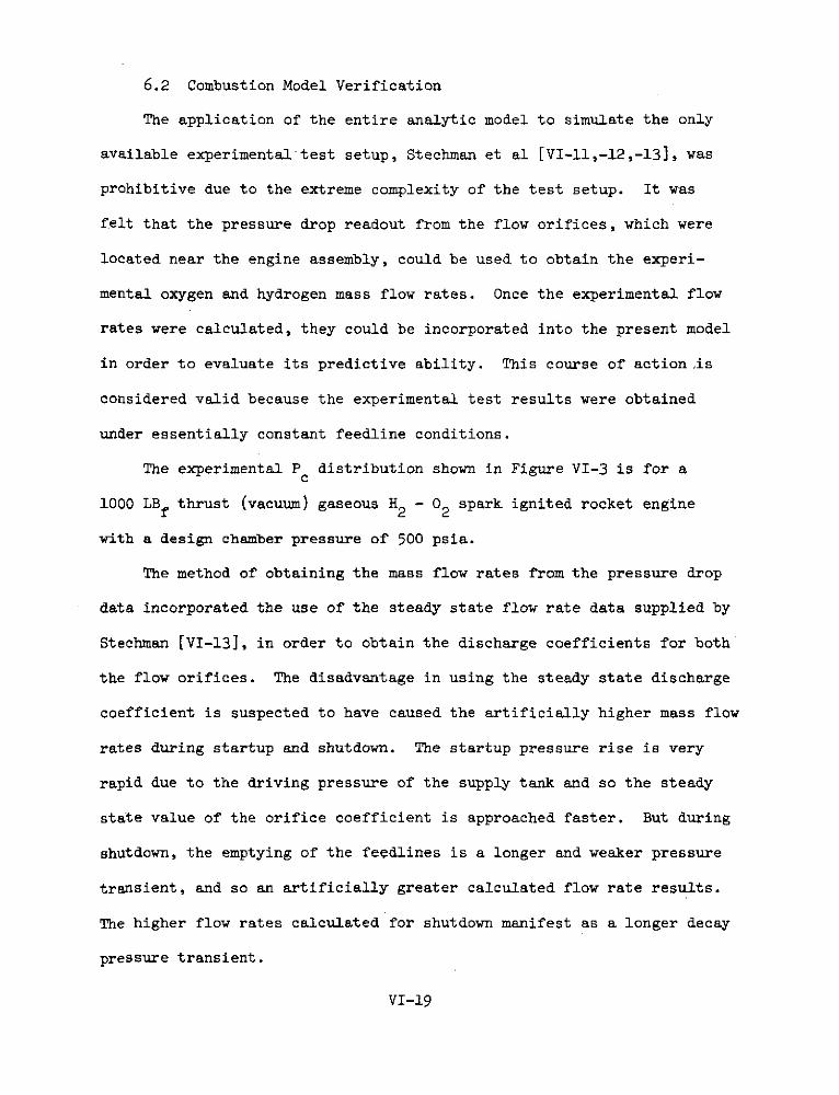
6.2 Combustion Model Verification
The application of the entire analytic model to simulate the only
available experimental test setup, Stechman et al [VI-11,-12,-13], was
prohibitive due to the extreme complexity of the test setup. It was
felt that the pressure drop readout from the flow orifices, which were
located near the engine assembly, could be used to obtain the experi-
mental oxygen and hydrogen mass flow rates. Once the experimental flow
rates were calculated, they could be incorporated into the present model
in order to evaluate its predictive ability. This course of action ,is
considered valid because the experimental test results were obtained
under essentially constant feedline conditions.
The experimental Pc distribution shown in Figure VI-3 is for a
1000 LBf thrust (vacuum) gaseous H2 - 02 spark ignited rocket engine
with a design chamber pressure of 500 psia.
The method of obtaining the mass flow rates from the pressure drop
data incorporated the use of the steady state flow rate data supplied by
Stechman [VI-13], in order to obtain the discharge coefficients for both
the flow orifices. The disadvantage in using the steady state discharge
coefficient is suspected to have caused the artificially higher mass flow
rates during startup and shutdown. The startup pressure rise is very
rapid due to the driving pressure of the supply tank and so the steady
state value of the orifice coefficient is approached faster. But during
shutdown, the emptying of the feedlines is a longer and weaker pressure
transient, and so an artificially greater calculated flow rate results.
The higher flow rates calculated for shutdown manifest as a longer decay
pressure transient.
VI-19

The ability of the theoretical model to predict the observed varia-
tion in chamber pressure during the startup transient and also the magni-
tude of the observed cver-pressurization warranted the conclusion that the
predictive ability of the combustion model is in good agreement with ob-
served data.
6.3 Effect of Manifold Volume
The design chamber pressure for both runs shown in Figure VI-4 is
100 psia, while the oxidizer and fuel manifold volumes for Runs 510 and
512 are 0.128 and 1.024 in. , respectively.
The chamber pressure distribution incorporates a time delay due to
ignition and combustion. The ignition lag time used for the majority of
the runs is based on the time required for the cold flow chamber pressure
to attain a value of 0.5 psia. The combustion lag time, (T), is composed
of a chemical reaction lag time and a mixing lag time. A constant value
of 0.05 ms was used for the chemical reaction lag time while the mixing
lag time could be either a constant or that prescribed by the mixing
model of Szuch. The combustion lag times for both runs of Figure VI-4
incorporate the gas mixing lag time of Szuch.
The variation in chamber pressure is seen to follow the correspond-
ing oscillations in mixture ratio. The initial fluctuations in mixture
ratio are caused by the fuel feedline pressure fluctuations, while the
larger oscillation in mixture ratio is caused by a compression wave
approaching and being reflected from the oxidizer propellant valve. The
manifold volume tends to have a strong influence on the startup tran-
sient. The effect of increasing the manifold volume by a factor of 8
VI-20

is shown to increase the chamber pressure rise and decay times by 85 and
70 percent respectively.
In the literature, the usual methods of determining the manifold
volume that is needed to feed the injectors entails multiplying the in-
jector flow area by a constant. The value three was chosen by Stechman
for the ratio of manifold volume to injector flow area because this value
provides the desired chamber pressure rise and decay rates while provid-
ing a reasonable volume for the manifolds.
6.4 Effect of Combustion Lag Time and Propellant Temperature
Figure VI-5 is composed of four separate runs, which incorporate
combustion lag times of 0.0 ms., mixing model of Szuch plus 0.05 ms.,
0.5 ms., and 0.75 ms. The mixture ratio distribution for the run in
Figure VI-5b is not shown since it is essentially identical to that of
run 560. The procedure is also followed in Figures VI-6 and VI-7.
In Figure VI-5a, the smoothness of this curve confirms the stability
of an instantaneous combustion case. The relative smoothness of the Pc
distribution in Figure VI-5b also predicts stable combustion for the
empirical mixing model of Szuch. The fluctuations in chamber pressure
are shown to increase with increasing combustion lag time. This observa-
tion is in agreement with the experimental observations of Crocco [VI-14].
The variations in chamber pressure caused by increasing T are evident in
the distortion of the mixture ratio distribution. The variations in mix-
ture ratio cause a corresponding variation in combustion gas temperature
which in turn causes the chamber pressure to vary.
VI-21

The low frequency Pc oscillations of 55 cycles per second (cps) in
Figures VI-5a, -5b, -5c, and -5d are caused by the oxidizer feedline
dynamics, which are known to be a function of feedline length and propel-
lant temperature. The high frequency oscillations suspected to be
caused by the magnitude of T and reinforced by a coupling between T and
the feed system sensitivity to P c. The above mentioned coupling is sus-
pected to have produced the Pc oscillations of 1000 and 665 cps in
Figures VI-5c and -5d, respectively.
The effect of reducing the propellant temperature by a factor of
0.8 and 0.4 is shown in Figures VI-6 and -7, respectively. By examin-
ing Figures VI-5, -6, and -7 in sequence, one notices that the instant-
aneous combustion case is inherently stable with increasing propellant
density, while the opposite is observed for larger T's. The Pc variation
exhibits an increase in the magnitude and duration of the high frequency
oscillations as T and the propellant density are increased. The pressure
sensitive feeding system, in responding to the chamber pressure fluctua-
tion initiated by the combustion lag, allows a greater mass flow fluctua-
tion through the orifice, due to the greater propellant density. This
type of trend is also documented by Feiler [VI-15] and Feiler and
Heidmann [VI-6].
'The high frequency oscillation in Pc shown in Figures VI-5c, -6c,
and -7c were approximately 1000, 800, and 665 cps with corresponding
chamber pressure variations of 4.5, 14, and 10 percent respectively. The
magnitude of the chamber pressure variations are based on the design
chamber pressure of 80 psia. By increasing T to 0.75 ms., the high
frequency oscillations in P shown in Figures VI-5d, -6d, and -7d were
c
VI-22

approximately 665, 665, and 570 cps, with corresponding chamber pressure
variations of 9, 9, and 12.5 percent, respectively. The low frequency
oscillations shown in Figures VI-5, -6, and -7 were 55, 49, and 37.5 cps
with a corresponding chamber pressure variation of 21, 19, and 15 percent.
The chamber oscillations shown in Figures VI-5, -6, and -7 may be
compared with the combustion instabilities observed in some rocket motor
tests. The experimentally observed combustion instabilities are known
to exist in two separate modes. One is a high frequency mode, with fre-
quencies ranging from 100 to as high as 5000 cps. The other mode is the
low frequency type, where the frequencies range from 10 to 100 cps.
If one considers the cylindrical combustion chamber as a simple
closed organ pipe, the fundamental frequencies for the longitudinal and
transverse direction would be 1860 and 7800 cps. Therefore, from the
range of high frequency Pc oscillation reported in the literature, one
may conclude that organ pipe type oscillations could be initiated and
reinforced by the predicted Pc oscillations of 1000, 800, and 665 cps.
Figure VI-8 illustrates the effect of combustion lag and propellant
temperature on the chamber pressure when the feedline dynamics are sup-
pressed, i.e., the upstream valve pressure is maintained at the steady
state design value. The results show that the chamber pressure distri-
bution becomes smoother, due to the steady mass flow from the propellant
valves, which tend to maintain a nearly constant mixture ratio of gas
flow into the combustion pressure-sensitive manifolds. Also, the high
frequency variations in chamber pressure were reduced in magnitude, thus
indicating that a coupling exists between the feedline dynamics and the
combustion lag time.
VI-23

The magnitude of the chamber pressure variation for T = 0.5 ms. is
reduced by a factor of 11.2 between runs 452 and 456, and 4.0 between
runs 252 and 256. The magnitude of the chamber pressure variation for
T = 0.75 ms. is reduced by a factor of 1.17 between runs 453 and 457,
and 1.92 between runs 253 and 257. Therefore, one can conclude that
even with a stable feedline system, i.e., operating at constant pressure,
Pc, fluctuations still exist if T is greater than 0.4 ms. Also, Figure
VI-8 confirms the in-phase coupling existing between the feeding system
and the Pc fluctuations, which tends to reinforce and increase the ob-
served P oscillations.c
The steady-state overpressurization of the runs shown in Figure
VI-8 is due to the sizing of the expansion nozzle for ideal flow conditions,
i.e., Cd = 1.0, whereas in the actual runs a Cd of 0.98 was used.
6.5 Effect of Shorter Feedline Lengths
Additional runs were made in order to determine the effect of feedline
length on chamber pressure oscillations.
The oxidizer and fuel valve pressures shown in Figure VI-9a infer
that the previously mentioned coupling between the feedline dynamics and
combustion lag is mainly a coupling of the fuel feedline dynamics and the
combustion lag time. Feiler [VI-15] reached this same conclusion. In
that the hydrogen flow is sufficiently sensitive, a coupling can exist
between the hydrogen flow oscillations and chamber pressure oscillations,
which can drive a combustion instability. Figure VI-9b verifies the above
statement by showing that if the hydrogen feedline length is sufficiently
VI-24

short and the feedline oscillations are damped out before combustion,
the previously noticed pressure fluctuations no longer exist. The fol-
lowing two figures, i.e., Figures VI-9c and -9d, represent the effect of
superimposing rapid fuel and oxidizer feedline pressure oscillations
early in the startup transient. The indication is that the coupling of
the fuel flow and combustion lag time initiates the high frequency
oscillations while the oxidizer side of the feeding system is responsi-
ble for the low frequency oscillations.
The area of combustion instability has been the object of many
publications, but at best, the analytical work is still of a qualitative
nature due to the complexity of the flow and reactions in a combustion
chamber. This study has not proposed a new or magic solution to the
problem of combustion instability, but has given a quantitative pers-
pective of the consequences of varying the design parameters, which are
qualitatively known to affect combustion stability. The present model
should enable a designer to obtain the relative importance of the various
parameters and eliminate or control combustion instabilities to improve
engine performance.
7. Conclusions
1) A gaseous bi-propellant RCS rocket engine is shown to exhibit
performance variations due to the pressure waves generated by the rapid
opening of the propellant valves. The pressure waves generated were
shown to be partially swallowed upon reflection from the valves and there-
fore damp out with time.
VI-25

2) Increasing the manifold volumes by a factor of 8 is shown to
increase the chamber pressure rise and decay times by 85% and 70%
respectively.
3) The effects of feedline pressure fluctuations, combustion lag
time, and propellant temperature on the chamber pressure are summarized
below.
a) The combustion process is inherently stable for T = 0.0, i.e.,
the chamber pressure does not exhibit rapid oscillations.
b) The incorporation of an empirical mixing lag time model was
shown to yield smooth combustion for a propellant temperature
of 500OR and somewhat rougher combustion with increasing
propellant density.
c) Increasing T and propellant density is shown to cause high fre-
quency oscillations in Pc which increase in magnitude and dura-
tion as T and propellant density are increased. The calculated
chamber pressure oscillation of 1000, 800, and 665 cycles per
second for r = 0.5 ms., is suspected to be the mechanism which
initiates the experimentally observed high frequency Pc
oscillation.
d) When the feedline pressure fluctuations are suppressed, the high
frequency variations in chamber pressure for T = 0.5 and 0.75
ms. were reduced in magnitude, thus indicating that a coupling
exists between the feedline pressure fluctuations and T.
yI-26

e) The low frequency P oscillations are shown to be primarily thec
result of the feedline pressure fluctuations, while the high
frequency oscillations, i.e., > 100 cps, are controlled by the
coupling between T and the fuel feedline system.
REFERENCES
VI-1 Summerfield, Martin, "A Theory of Unstable Combustion in Liquid
Propellant Rocket System", J. Am. Rocket Soc., Vol. 21, No. 5,
Sept. 1951, pp. 108-114.
VI-2 Crocco, Luigi and Cheng, Sin-I, "Theory of Combustion Instabilites
in Liquid Propellant Rocket Motors. AGARDograph No. 8, Butterworth
Sci. Pub. (London), 1956.
VI-3 Crocco, L.; Grey, J. and Harrje, D. T., "On the Importance of the
Sensitive Time Lag in Longitudinal High-Frequency Rocket Combus-
tion Instability", Jet Propulsion, Vol. 28, No. 12, p. 841, 1958.
vI-4 Szuch, J. R., "Digital Computer Program for Analysis of Chugging
Instabilities", NASA TND-7026, 1970.
VI-5 Hersch, Martin, "A Mixing Model for Rocket Engine Combustion",NASA TND-2881, 1965.
VI-6 Feiler, Charles E.; Heidmann, Marcus F., "Dynamic Response of
Gaseous-Hydrogen Flow System and its Application to High-FrequencyCombustion Instability", NASA TND-4040, 1967.
VI-7 Eschweiler, J. C.; Wallace, H. W., "Liquid Rocket Engine Feed
System Dynamics by the Method of Characteristics", ASME Annual
Aviation and Space Conference, Beverly Hills, California, June
16-19, pp. 271-280, 1968.
VI-8 Sidransky, F. S. and Smith, M. M., "Nonsteady Liquid and GasFlow with Heat Addition and Shock Perturbation", NASA TND-3684,
Oct. 1968.
VI-9 Markowsky, J. J., "An Analytical Model for Predicting the Pressureand Flow Transients in a Gaseous H - 02 100 LB Thrust Reaction
Control Rocket Engine", Ph.D. Thesis, Cornell University, Ithaca,N. Y., 1971.
VI-10 Gordon, S.; McBride, B. J., "Theoretical Performance of LiquidHydrogen with Liquid Oxygen as a Rocket Propellant", NASA Memo-
randum 5-21-59E, 1959.
VI-27

VI-11 Stechman, R. C., et al,"GH /GO2 1,000 lbf Thrust Rocket EngineTest Program, P/N X25650, 2MIR #365, The Marquardt Corp., Van
Nuys, Calif., April 1970.
VI-12 Stechman, R. C., Personal communication, The Marquardt Corp.,Van Nuys, Calif., August 11, 1970.
VI-13 Stechman, R. C., Personal communication, The Marquardt Corp.,Van Nuys, Calif., March 16, 1971.
VI-I4 Crocco, L., "Aspects of Combustion Stability in Liquid Propel-lant Rocket Motors, Part I", ARS Journal, November 1951,pp. 163-178.
VI-15 Feiler, C. E., "Effect of Combustion Parameters on the Stabilityof Gaseous Hydrogen-Liquid Oxygen Engine", NASA TMX-52360, 1967.
NOMENCLATURE
A Cross-sectional area when subscripted with v, o, or i, non-
dimensional acoustic velocity when not subscripted or when
subscripted with r or T only.
a Acoustic velocity.
c Constant pressure specific heat.p
cv Constant volume specific heat.
d Diameter of feedline.
D Diameter.
E Enthalpy of gas.
F Thrust.
g Dimensional constant.
J Dimensional constant.
L* Characteristic chamber length.
L Feedline length.
M Molecular weight.
VI-28

MR Mixture ratio.
m Mass.
m Mass flow rate.
n Polytropic exponent.
P Pressure.
Riemann invariant, (wave moving with the flow).
Q Riemann invariant, (wave moving against the flow).
R Gas constant.o
T Temperature.
t Time
tstart Time when valve begins to open.
tstop Time when valve begins to close.
At Computing time interval.
U Nondimensionalized velocity.
u Velocity.
V Volume.
x Axial distance.
y Ratio of specific heat.
p Density.
t Combustion time delay.
Subscripts
c Refers to combustion chamber.
cf Refers to fuel in combustion chamber.
ci Refers to initial mass in combustion chamber.
co Refers to oxidizer in combustion chamber.
VI-29

CT Refers to chemical reaction temperature
CTT Refers to theoretical combustion temperature.
c* Refers to characteristic exhaust velocity efficiency.
d Refers to downstream.
F Refers to fuel.
i Refers to injector.
if Refers to fuel at injector.
ifi Refers to initial mass at fuel injector.
io Refers to oxidizer at injector.
ioi Refers to initial mass at oxidizer injector.
m Refers to manifold.
n Refers to nozzle.
ne Refers to nozzle exit.
nt Refers to nozzle throat.
o Refers to orifice or valve.
O Refers to oxidizer.
P Refers to propellant (oxidizer and fuel).
r Refers to reference condition.
T Refers to tank.
t Refers to throat.
u Refers to upstream.
V Refers to valve.
VF Refers to fuel at valve.
VO Refers to oxidizer at valve.
VI-30
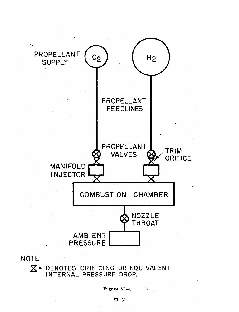
PROPELLANT 02 H2SUPPLY
PROPELLANTFEEDLINES
PROPELLANTVALVES / RIM
,F ORIFICEMANIFOLDINJECTOR
COMBUSTION CHAMBER
NOZZLETHROAT
AMBIENTPRESSURE
NOTE
A= DENOTES ORIFICING OR EQUIVALENTINTERNAL PRESSURE DROP.
Figure. VI-1
VI-31

(a ... 30 (a) Pc DESIGN 100 PSIA RUN 500
I) 20
a.u 10a
0
I - - -,100 (b)
<C F
a-80-
w
0U-
o 6 (c)
w
S I2
S20
Figure VL-2. Cold flow run.
VI-32VIr32

(a) - THEORY---- RUN 76 OF REF. (26)
240. RUN 501240 - / _ .. .
200 -
160
120 -
a)
S• I I\.I.
a80
I 40 4
00 20 40 60 80 100 120 140 160TIME-MILLISECONDS (MS)
* I ' I ' I ' I ' I ' I ' I(b) DURATION OF. SPARK CURRENT
RUN 76 OF REF.. (261-...
THEORY
0 20 40 60 80 100 120 140 160
TIME-MILLISECONDS (MS)
Figure VI-3. Analytical combustion model verification.
VI-33
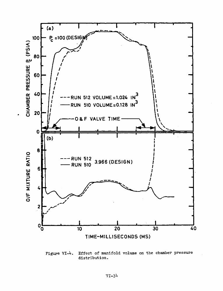
(a)
100 P =100 (DESIG
80
560do ; ti
w
e 40 3w I --- RUN 512 VOLUME=1.024 IN2 I - RUN 510 VOLUME=0.128 IN |
< 20 I \i -- 0 &F VALVE TIME
0
(b) I
I
8 IO II--- RUN 512 I< 3.966 (DESIGN) I0 10 RUN 51030 40
61-3h
o 2
0 10 20 30 40
TIME-MILLISECONDS (MS)
Figure VI-4. Effect of manifold volume on the chamber pressure
distribution.
-vI-34

-=0o
.o M
S '
'=M
IXIN
G
OD
z80
t=
0.2
5,0
/F =
17
.6)
OF
REF
.(9
1.0
(a)
(b)
U
60
P
RU
N
560
-RU
N 50
2 -
0.8
6.0
' o
7d
o 20
-
0.4
2.0
-O
& F
VAL
VE
TIM
E
, '.-
....
---
_ -.
......
..
I~I-
o d
.
0.2
0.0
o0
0
60
U
=0.5
M
S cf
.35-
M
" o
0 a.
I.
F
OD
0
0.4
o2.0
W
O&
F
VALV
E T
IME
M
II
-: -
,-0w
80
- (
1-b
p
0 (c
) (d
)
00
w 62
.0
00
10
20
0
10
20T
IME
-MIL
LIS
EC
ON
DS
(MS)

z
'==
0.0
MS
'=
MIX
ING
M
OD
E80
O
F R
EF. (
9)
1.0o
(t:0
.25,O
IF17.
(a)
b)
P6
RUN
450
RUN
451
60
-
ID
<
0d
w
40
-
0/F
'.
0.6
< 4
.0
n
o
U0
-0.
4 2.0
a. L
mP 0
c
O&
F V
ALV
E
TIM
E
CD
"
<
I-
0.2
0 0.0
S
0
.,.-=o0.5
MS
s
=/.-"
M(D,0
O-, W
RUN 452
RUN
45
3a
60 -
o
So
"
X , ....
40 L
OL
F
4.0
&
40
ci-
W
0.0
o0 0
10
20
0 10
20
TIME-MILLISECONDS (MS)

zr7
=0.0
M
S 4
r= M
IX I
6 M
OD
EL
o80
O
F R
EF.
(9)
1.0
t n
S60
(a)
(b)
0.8
6.0
I R
UN
250
R
UN
25
1 o
OId
t N
I
-40
,
-0.6
4.
0 "
C 'O
20
--
0.4
2.0
x
o L
" 0
, 0.
2 U
0.0
o
C+O
L
7 =0
.5
MS
I"=
0.75
M
S
0
60
(c)
(d)
6.0 o
P <
RU
N
252
RU
N
253
!
OF
-
s 20
-
2.0
0 0.
0 o
0 10
20
0
10
20
TIM
E-M
ILLI
SEC
ON
DS
(MS)

60C
, I
ST
= 4,
00o
R
ITp
=40
00 R
40 -
RU
N 4
55--
---
'r=O
.O
MS
-R
UN
455--
---
r=O
.O M
S+
.I
RUN 456--r'=0.5
MS
RUN
457-
- =0.75
MS
I I
o
o H
"a.
(c
) -
(d)
u/0,/
<'
P.6
0
p I
pT2
T =
2000
R40
-R
UN
255--
---
=0.0
M
S I
RU
N
255
----
- r=
0.0
M
SIC
R
UN
256
-=0
1.5
MS
RU
N
257
--r=0.75 M
SI
-
20 0
10
20
0 10
20
TIM
E-M
ILLI
SE
CO
ND
S
(MS)

80
(a)
(b)
RU
N
452
RU
N
471
C6-
-
-"
140
p I
R
130
Z-
<
40
110
o I
Lo=
5.0 F
EET
Lo=5
.0 FE
ET
110
W"
u
20*
LF=
5.0
FEE
T
LF
0.5
FEE
T
100
m
w
7'=
0.5
MS
T=
0.5
MS
U)
0 a:
O
&F
VA
LVE
TIM
E
90
wV
I) a
*
a. 8
0 (c
) (d
)<
SRU
N
472
RU
N
473
CO P
A60
-
-140
<P
. C
a
PV
/ \
" 13
0 -
Svo
110
4 -o
= 2
.5
FEE
T
Lo
2.5
FE
ET
20
= 2.
5 FE
ET
L
=5.
0 FE
ET
-
100
l"=
0.5
MS
'=0
.5 M
S 90
0
10
20
0 10
20
TIM
E-M
ILLI
SE
CO
ND
S
(MS)

Chapter VII: Electrical Power System
1. Introduction
The LSV power subsystem generates, stores, and controls electrical
power for distribution to the spacecraft subsystems. The energy require-
ments are based on a round-trip mission time of four hours - two and a
half hours for descent from Lunar orbit to Lunar surface and one and a
half hours for ascent from Lunar orbit to docking with orbiting Lunar
base. The design of the LSV is based on deployment in the 1978-1985
time period and includes a permanent base in Lunar orbit which will
provide refueling and refitting facilities for the shuttlecraft. While
docked with the Lunar orbit base, or by the Lunar base, the LSV power
will be drawn from the respective base. The concept of reusability and
refittibility is a major consideration in selecting an electrical power
system.
Except in the propulsion field, probably no other systems are being
developed over such a broad spectrum for spacecraft applications as are
electrical power generation systems. This is especially true for manned
spacecraft applications where power requirements are significantly higher
than for most unmanned payloads.
Three sources of energy are available for conversion to electrical
power on spacecraft: chemical, solar, and nuclear. Systems which utilize
each type of energy source have been developed and flown in this country's
space program. Chemical energy may be stored in self-contained packages,
with batteries, as an example, or it may be supplied in the form of a
fluid or fluids from external subsystems which are consumed in the energy-
conversion system, e.g., fuel cells. Photovoltaic or solar cells have been
VII-1

used successfully on numerous scientific unmanned missions. The third,
and equally successful, conversion technique used in some unmanned
spacecraft has been th'e radioisotope-fueled thermoelectric generator.
It should be noted, however, that most of these applications have re-
quired less than 100 watts of power. The Mercury spacecraft provided
one exception to this rule - it used on the order of 500 watts maximum
power for what ultimately turned out to be a 3h-hour mission.
Thus, with the previously mentioned candidate power systems only
batteries and the fuel cells will be considered due to the recharge
frequency and energy requirements of the LSV. The LSV's power system
will supply energy at a nominal 29 volts DC. Alternating current power
can be supplied either from a central power conditioner or from indivi-
dual subsystem power conditioning devices.
2. Power System Requirements
Table VII.1 provides a summary of the ascent and descent power and
energy requirements for one round-trip mission of the LSV. The duty times
used as the basis for the estimation of the energy requirements are also
shown in the table. Also, the load requirements are based on 1970 tech-
nology and therefore will be conservative with the expected advances in
the guidance, navigation, and environment control areas.
The total electrical energy requirements for a round trip from Lunar
surface to Lunar orbit and back again are 6742 w-hrs. Adding ten per-
cent for wiring and conversion losses results in an energy requirement of
7416 w-hrs. During the mission the power requirements are maintained at
a nearly constant level of 2,000 watts with peaking occurring at a level
of approximately 2500 watts.
VII-2
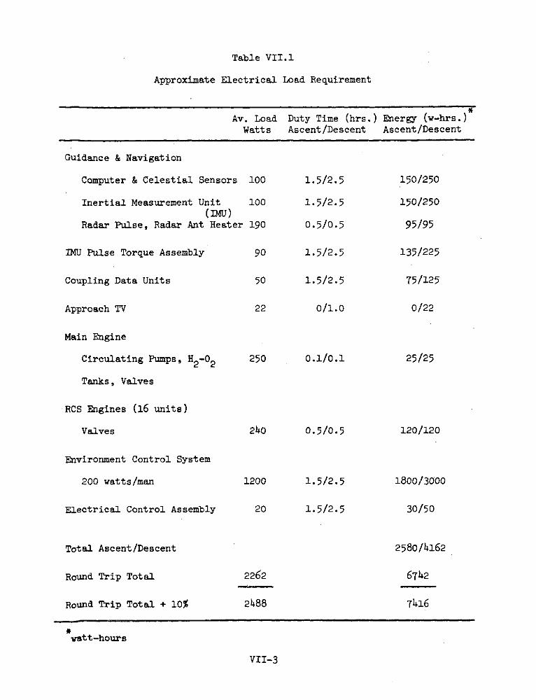
Table VII.1
Approximate Electrical Load Requirement
Av. Load Duty Time (hrs.) Energy (w-hrs.)
Watts Ascent/Descent Ascent/Descent
Guidance & Navigation
Computer & Celestial Sensors 100 1.5/2.5 150/250
Inertial Measurement Unit 100 1.5/2.5 150/250(IMU)
Radar Pulse, Radar Ant Heater 190 0.5/0.5 95/95
IMU Pulse Torque Assembly 90 1.5/2.5 135/225
Coupling Data Units 50 1.5/2.5 75/125
Approach TV 22 0/1.0 0/22
Main Engine
Circulating Pumps, H2-02 250 0.1/0.1 25/25
Tanks, Valves
RCS Engines (16 units)
Valves 240 0.5/0.5 120/120
Environment Control System
200 watts/man 1200 1.5/2.5 1800/3000
Electrical Control Assembly 20 1.5/2.5 30/50
Total Ascent/Descent 2580/4162
Round Trip Total 2262 6742
Round Trip Total + 10% 2488 7416
watt-hours
VII-3

2.1 Payload Support
Payload support has been incorporated in the power system load require-
ments. The environmental control system requirements are 200 watts/man,
with a maximum of a six man payload allotted. If a fewer number of men
are included in the payload, residual power of 200 x (6 - number of passen-
gers) watts can be used for payload support.
3. Candidate Power Systems
Two alternate power systems have been considered and evaluated. The
following paragraphs provide a description of each of the systems.
a) Batteries
Secondary batteries are simply those in which the components are com-
patible with each other; that have reasonably good stand life in the
conditions under which they may be stored (with or without a trickle charge),
that undergo few, if any, chemical side reactions and thus show high current
efficiency, and can, therefore, be electrically recharged.
There are three types of secondary batteries, i.e., designated to be
charged and discharged many times:
cycles watt-hours/Lbm1) Nickel-cadmium 10,000 15
2) Silver-cadmium 10,000 (approx.) 25
3) Silver-zinc 500 (approx.) 60
The above cycle life times are based on depth of discharge of the order of
20 to 25%, which are currently used in space. Future improvements will
yield similar cycle life for a depth of discharge of 30% [VII-6].
The advantage of the nickel-cadmium couple over other secondary
batteries include small voltage excursions, high rate charge acceptance,
See References.vII-

long shelf. life, and low temperature operation. The silver-cadmium
secondary battery approaches the long life of the nickel-cadmium and the
high energy density of-the silver-zinc batteries. The silver-cadmium
cells have approximately twice the energy density of the nickel-cadmium
and a cycle life 1 to 2 orders of magnitude greater than the silver-zinc
cell which may be outweighed, for many applications, by the low cell
voltage regulation [VII-2]. Because they may be charged more rapidly
than silver-zinc cells, silver-cadmium cells are useful when rapid
repetition of cycles is required.
The silver-zinc secondary battery is the highest energy density
battery in common use. However, it does not yet have the good cycle
life of the nickel-cadmium battery. Silver-zinc cycle life is still
measured in hundreds of cycles as compared with thousands of cycles for
the other two.
For the battery candidate power source, silver-zinc batteries
were selected based on simplicity, reliability, proven design, high energy
output per unit weight, high peak-current capability, and reusability.
The disadvantages of silver-zinc cells are their relatively short useful
lifetimes (approximately 500 cycles at 30% depth of discharge) and their
limited temperature range of -55 0 F to +100 0F.
The total electrical energy requirement for a battery power system
design for 30% depth of discharge for one round trip mission is 24,700
watt-hours. The total battery weight required would be 412 pounds. A
three battery arrangement would provide a safety margin even if two
batteries fail. Each battery would weigh 137 lbm and have 20 cells.
This specification is almost identical to the descent battery used in
the LEM [VII-31.
VII-5

b) Fuel Cell
A fuel cell is an electrochemical device in which energy is derived
from a continually-supplied chemical reaction and is converted directly
into electrical energy.
Candidate fuel cells are as follows:
1) Pratt & Whitney Aircraft, Type PC8B-3, 2KW, 105 watts
parasitic load weight: 104 pounds per module, liquid
cooled [VII-h].
2) Allis-Chalmers, 2KW, capillary matrix type, gas/liquid
cooled, weight: 169 pounds per module, 100 watts parasitic
load [VII-5].
Three fuel cells are required to offer the same redundancy as for
the all battery system, i.e., two may fail without endangering mission
success.
h. Power System Comparison
The addition of further discussion on fuel cells or possible fuel
cell and battery combination is not persued due to the particular type
of power requirement needed for the LSV. The LSV will be used for supply-
ing the lunar base at regular or irregular intervals and also for explora-
tion of the moon. Therefore, the LSV will be dormant most of the time,
and used for regular scheduled and emergency missions. Fuel cells are
designed primarily for continual operations, with a power down mode.
Between five or six hours and, say,three months of service, fuel cells
usually show higher energy densities than batteries. But, because of
more difficult storage of reactants and of need for removal of products,
VII-6

the total system is more complicated. So, for a mission time of less
than five hours and on-off operation, fuel cells are not as feasible as
static batteries [VII-6].
The fuel cells system weight is approximately 595 lbs whereas the
equivalent battery system weight is 511 lbs. The volume of the three
batteries would approximate 1/6 that of the fuel cell combination. The
fact that the LSV vehicle can be refitted and also have batteries
recharged indicates that batteries are more feasible from the viewpoint
of weight and volume. Therefore, three batteries composed of silver-
zinc plates with 20 cells a piece and a potassium hydroxide electrolyte
are proposed. Silver-zinc batteries are usually tailormade and therefore
no single standard line of cell has evolved. Because of the variation in
cell structure details and the consequent performance variations, virtu-
ally no parametric performance data exists outside of the manufacturer's
hands.
5. Design Data Requirements
The requirements of battery-operated-characteristics data depends
upon the electric-power-system design in which the batteries are used.
A relatively simple and conservative design system generally requires a
minimum of detailed operating-characteristic data. As the design
becomes more sophisticated and the requirements for high-efficiency
storage and utilization of source energy becomes more critical, the
requisite amount and accuracy of battery characteristic data, i.e.,
voltage versus time or current versus time curves, increase. The data
required for the final design is:
VII-T

1) Discharge voltage as a function of time under the actual load
conditions expected.
2) Charge voltage and current as a function of time under the
actual charging conditions expected. If the charging conditions
are unknown, the battery data should contain enough information
to derive the charging current and voltage required.
3) Quantity of electrical energy available from the battery at
certain critical points in the mission, and the assurance that at
all other periods the energy availability exceeds the requirements.
4) Rate of heat evolution as a function of time under the actual
charge and discharge conditions expected, and a complete tempera-
ture profile of the battery as a function of time.
5) Impedance and phase-shift characteristics of the battery as a
function of frequency.
6) Efficiency of the battery's energy storage and its associated
electronics.
7) Probability of battery failure as a function of time and condi-
tions of use.
8) Battery voltage transients for critical load changes.
Most, if not all, of the above data requirements depend upon system-
design concepts as well as environmental variables such as temperature,
charge and discharge currents, and system-load characteristics and speci-
fications (which vary with the changing spacecraft design and mission).
VII-8

REFERENCES
VII-1 Performance Forecast of Selected Static Energy ConversionDevices, 29th Meeting of Agard Propulsion and EnergeticsPanel, Liegel, Belgium, June 12-16, 1967.
VII-2 Bauer, Paul, "Batteries for Space Power Systems", NASASp-172, 1968.
VII-3 Apollo Operations Handbook, Lunar Module LM 7 and subsequentVolume I Subsystems Data, LMA 790-3-LM 7, Grumman AerospaceCorp., New York, February 1970.
VII-4 Pratt and Whitney Aircraft, "Fuel Cells for LM- DerivativeSpacecraft", Ref. No. 69-1287, prepared for Grumman AircraftEngineering Corp., March 19, 1969.
VII-5 Improved Lunar Cargo and Personnel Delivery System, Volume111A: Conceptual Design and Subsystem Analysis, LockheedMissiles and Space Co., Sunnyvale, California, ContractNAS 8-21006, June 1968.
VII-6 Manned Spacecraft, Engineering Design and Operation, Editedby Purser, P. E.; Faget, M. A.; Smith, N. F., FairchildPublications, New York, 1964.
VII-9

Chapter VIII: Landing Gear Design
1. Introduction
The major emphasis of lunar landing gear design activity has been
directed toward designing effective means of vehicle arrestment and
stabilization for two vehicles, the Surveyor and the LEM. Consequently,
the development of systematic landing gear design procedures which would
be applicable to a wide range of landing vehicles has not been necessary.
However, as further exploration and eventual colonization of the moon
take place, the need for a wide range of reusable landing vehicles has
been predicted. The objective of this chapter is to develop a systematic
landing gear design method which could be applied, in general, to reusable
lunar landing vehicles.
Lunar landing gear systems design consists of developing design
criteria and concepts of vehicle arrestment and stabilization so as to
achieve some mission objective. U.S. designers' conceptions of space-
craft capable of controlled, soft landings on the moon have been charac-
terized by vehicles with legs. The legs, which have been trusses with
built-in energy absorbers, are designed to prevent damage to craft and
crew during the landing impact, and to bring the vehicle to rest in an
upright attitude. For a given design concept, sub-optimal landing gear
systems design involves choosing values for the design parameters such
that the solution will be "best" based on some performance criteria.
The design iteration cycle consists of selecting initial design para-
meter values, determining if this solution satisfies the design criteria,
and choosing new parameter values to "improve" the solution consistent
with the design criteria.
VIII-1

The design method developed in this study applies a digital simula-
tion of the landing vehicle to generate a solution surface, and a con-
strained optimization algorithm to locate the local optima on this
surface. An initial design solution is supplied to the simulation-
optimization routine and serves as a starting point for the optimization
procedure which eventually leads to an approximate mathematical locally
optimal design solution. Different starting points lead to alternative
locally optimal designs, from which a "best" design is chosen based on
vehicle performance characteristics.
The mathematical model of the system consists of an objective
function, system constraints which result from the design criteria, and
a digital simulation which determines vehicle performance characteristics
for specific design parameter values. The optimality of the mathematical
local optima, with respect to the real local optima, depends on the accu-
racy and completeness of the model and the relative optimality of any
arbitrary design assumptions. Thus, an optimal solution of a model involv-
ing only the major design parameters of a system is mathematically sub-
optimal unless all secondary design parameters have been fixed, by chance,
at optimal levels.
2. Problem Definition
The landing vehicle-landing site system is described by three
basic types of parameters: those involving the vehicle, those para-
meters describing the landing gear, and those parameters describing the
landing conditions. See Table VIII.1. The landing gear design variables
are those system parameters over which the designer has control. The
VIII-2

Table VIII.1
VEHICLE PARAMETERS
Mass
Moments of Inertia
Geometry
Mass Distribution
LANDING GEAR DESIGN PARAMETERS
Number of Gears
Geometry (size, orientation, etc.)
Location of Hardpoints
Location of Footpads
Stroking Characteristics of Energy Absorbers
Mass of Energy Absorbers
Size of Footpad
Mass of Footpad
LANDING CONDITION PARAMETERS
Surface Slopes
Soil Characteristics
Surface Roughness (protrusions, indentations, etc.)
Vertical Velocity
Horizontal Velocity
Pitch, Yaw, Roll
Pitch Rate, Yaw Rate, Roll Rate
VIII-3

other parameters are either fixed (mass, moments of inertia, etc.) or
are random variables (initial touchdown conditions). A landing gear
systems design involves selecting values for the thirty or more design
variables so that the solution satisfies the design criteria for the
fixed system parameters and for the designated ranges of touchdown
parameters. If only three values for each design variable are con-
sidered, a total number of 330 = 2.05 x 10¹⁵ design combinations must
be evaluated. Since one simulation run requires approximately five
seconds of computer time, the total time required to evaluate all
design combinations is approximately 3.2 x 10⁷ years.
2.1 Landing Gear Design Criteria
Landing gear design criteria define the limits of the landing
conditions for which the vehicle will land with a particular outcome.
For example, one design criterion might specify the limits of the
initial landing conditions for which no crew injury or craft damage
should occur. An alternate criterion might set limits on the initial
landing conditions for which slight crew injury and craft damage would
occur. These limits on the initial landing conditions can be thought
of as related to confidence limits of the random variables involved,
even though the distributions of these variable have not been discussed
in the literature.
2.2 The Constraint Set
The system constraints are limits on the vehicle performance
characteristics which result directly from the design criteria. For
example, the design criteria involving no crew injury may be translated
VIII-4

to limits on maximum vehicle deceleration. Similarly, a vehicle stability
constraint may correspond to the design criteria pertaining to vehicle
damage or final attitude. Thus, the landing gear design criteria become
constraints on the vehicle design variables and performance character-
istics which are not to be violated for a given range of initial landing
conditions.
2.3 Design Model Objective Function
In general, a set of design criteria may be satisfied by more than
one design solution. It is therefore desirable to develop a criterion
so that the "best" solution can be determined. This criterion may be
expressed mathematically in the form of an objective function which is
to be minimized or maximized during the optimization process. For
example, one logical design objective is that of minimizing total vehicle
cost. Another objective might be minimizing total landing gear weight.
Still another design objective might be maximizing the range of initial
landing conditions for which the vehicle can land successfully.
3. Landing Gear Design: An Optimal Solution
The landing of a lunar vehicle is a probabilistic event in that
the landing conditions vary from site to site and the vehicle touch-
down parameters are random variables dependent on the pilot and the
guidance equipment. An optimal solution for this probabilistic problem
**is a solution which is feasible for all anticipated combinations of
landing conditions and which is "best" in some sense.
In general, there are two basic system models: the deterministic modeland the probabilistic model. The former differs from the latter in thatthe latter is characterized by the existence of one or more random systemvariables.**A feasible solution is one that violates none of the constraints.
VIII-5

Optimal landing gear design solutions are approximated in the
literature by determining locally optimal design solutions for several
"worst case" combinations of landing conditions. The reliability of
each design is then evaluated by checking its feasibility for many
other combinations of initial conditions . The optimal solution is the
"best" solution of this group based on considerations such as the value
of the objective function and the reliability of the design.
A major area of landing gear design difficulty involves deter-
mining the "worst case" initial landing conditions for which an optimal
solution is to be determined. Since the "worst case" conditions are
not independent of the specific gear design, their calculation becomes
a trial and error process. While the optimization process is compli-
cated when more than one "worst case" landing gear combination exists,
an additional problem occurs when the locally optimal solutions for any
one set of initial conditions are infeasible for other "worst case"
combinations. When such difficulties arise, the concept of design
reliability becomes necessary. The reliability approach is limited,
however, because it is impractical to test the feasibility of a solution
for all anticipated initial condition combinations. Thus, the relia-
bility of a design is usually only estimated.
*The reliability of a design is the number of combinations of initial
landing conditions for which the design is feasible divided by the totalnumber of possible initial condition combinations.
**eIdeally, a solution that is feasible for a "worst case" set of landing
conditions will be feasible for all anticipated landing conditions.
VIII-6

4. Study Objectives and Design Assumptions
A complete landing gear design study involves some broad trade-off
analyses. For example, there is the conceptual trade-off between an
energy absorbing landing gear system which is attached to the vehicle
and an energy absorbing landing platform located at each landing site.
Other trade-off studies might involve the cost of improving the guid-
ance equipment to a point where an unsophisticated, non-energy absorb-
ing landing gear system would be sufficient. Such studies are, however,
lengthy and beyond the scope of this analysis. The landing gear concept
used in this study is an extrapolation from the present LEM design in
that the shock absorbers are reusable. The vehicle control capabilities
have also been updated.
The primary objective of this study is to develop a computerized
approach for approximating locally optimal landing gear design solutions
for mathematical models of lunar landing vehicles. Mathematical pro-
gramming techniques will be used to approximate locally optimal solutions
for specific initial landing conditions for constrained models of two,
three, and four design parameters. The effect on these solutions to
changes in initial landing conditions will then be evaluated. Vehicle
stability and crew safety will be the design criteria from which the
constraint set is developed. A three-dimensional digital simulation of
the landing vehicle will be used to determine design performance results.
The vehicle mass, dimensions, and moments of inertia used in this
analysis are consistent with preliminary estimates of those of the
proposed lunar shuttle vehicle. See Table VIII.2. The geometry of the
proposed vehicle is shown in Figure VIII-1.
VIII-T

Table VIII.2: Vehicle Design Variables
Vehicle Mast 400 slugs
Moments of Inertia 8000 slug-ft2
X-direction Velocity 4 ft/sec
Y-direction Velocity 0 ft/sec
Z-direction Velocity -2 ft/sec
Pitch +50
Roll 00
Yaw 00
Pitch Rate +0.1 rad/sec
Roll Rate 0 rad/sec
Yaw Rate 0 rad/sec
R/H 0.75
Gravity Vector 0,0, -32/6(zero slope)
Tangential Soil Coefficient 0.00001
Vertical Soil Coefficient 0.00001
Strut Extension Force 1000 pounds
Maximum Stroke ±1.25 ft.
Elastic Range of Strut 0.003 ft.
VIII-8

Due to the large number of design parameters, it is impractical to
treat each as a design variable. Therefore, the design parameters of
compressive strut force and landing gear radius are chosen as design
variables while the other design parameters are fixed at levels con-
sistent with previous study results. The compressive strut force is
the force at which continuous contraction of the landing gear strut
occurs. The gear radius, R, is shown in Figure VIII-1. Studies by
Black (12), NASA-ASEE (2), and Lockheed (3) indicate these parameters
to be of major importance in landing gear design.
4.1 Landing Gear Design Assumptions
The landing gear system chosen for the shuttle craft consists of
a three gear, inverted tripod design. See Figure VIII-2. Landing gear
studies by Black (8) and Bendix (1) indicate that the optimum number
of gears depends primarily on gear weight and that both the three
and four gear systems have resulted in successful designs. The three
gear design was chosen in this study for the following reasons:
1. The present study attempts to optimize the forward two gear
designs and assumes -a front-foot-touchdown landing . Thus,
the design of the rear gear(s) is of secondary importance.
2. The digital simulation of a three gear design costs approxi-
mately one-fourth less than one of a four gear design.
Two basic gear leg configurations are presented in the literature:
the cantilever configuration and the inverted tripod configuration.
See Figure VIII-3. Mantus (13) reports that the cantilever design is
Landing gear design consists of designing for front-foot-touchdownand rear-foot-touchdown landing conditions. This work only considersthe first of these two cases.
VIII-9

superior to the inverted tripod configuration. A Bendix report (1)
suggests that the inverted tripod design might be optimal for certain
unspecified conditions. In the present study, the inverted tripod
gear design was arbitrarily chosen over the cantilever design primarily
to reduce the complexity of the simulation. Each inverted tripod is
made up of three energy absorbing struts which act as columns with
pinned ends. The struts are designed to extend or contract a maximum
of 1.25 feet from the original length. The constant force-deflection
characteristics of the energy absorbers are similar to those of the
crushable honeycomb cartridges used in the LEM design. Since the shut-
tle craft requires a reusable landing gear system, an energy absorber
similar to the NASA, MSFC Friction Shock Absorber is indicated (1T).
See FigureVllk.This reusable energy absorber is designed to produce
a constant force-deflection characteristic.
The location of the footpads and the strut attachment points on
the vehicle (the hardpoints) were chosen so as to result in the opti-
mal tripod configuration as reported by Bendix (1):
1. The secondary struts should be symmetric about the primary
strut and of the same length.
.2. The angle of the primary strut should be 30 degrees from the
vertical.
The mass of the struts, energy absorbers, and footpads are negli-
gible compared to the mass of the vehicle and are neglected in the
digital simulation of the craft. The size of the footpad and the soil
characteristics are such that a pinned foot condition holds
When a footpad is in contact with the surface, it is assumed to bepinned until there is a tendency for it to lift off.
VIII-10
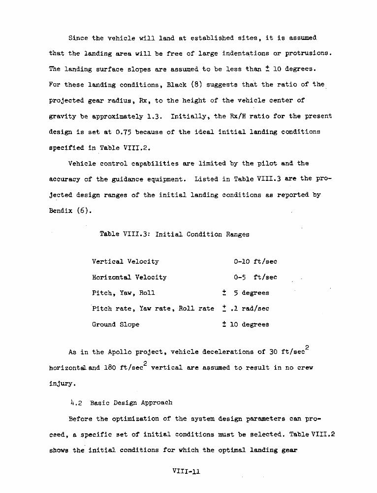
Since the vehicle will land at established sites, it is assumed
that the landing area will be free of large indentations or protrusions.
The landing surface slopes are assumed to be less than ± 10 degrees.
For these landing conditions, Black (8) suggests that the ratio of the
projected gear radius, Rx, to the height of the vehicle center of
gravity be approximately 1.3. Initially, the Rx/H ratio for the present
design is set at 0.75 because of the ideal initial landing conditions
specified in Table VIII.2.
Vehicle control capabilities are limited by the pilot and the
accuracy of the guidance equipment. Listed in Table VIII.3 are the pro-
jected design ranges of the initial landing conditions as reported by
Bendix (6).
Table VIII.3: Initial Condition Ranges
Vertical Velocity 0-10 ft/sec
Horizontal Velocity 0-5 ft/sec
Pitch, Yaw, Roll ± 5 degrees
Pitch rate, Yaw rate, Roll rate 1 .1 rad/sec
Ground Slope ± 10 degrees
As in the Apollo project, vehicle decelerations of 30 ft/sec 2
horizontaland 180 ft/sec2 vertical are assumed to result in no crew
injury.
4.2 Basic Design Approach
Before the optimization of the system design parameters can pro-
ceed, a specific set of initial conditions must be selected. Table VIII.2
shows the initial conditions for which the optimal landing gear
VIII-11

solutions will be determined. A touchdown velocity vector of 4 ft/sec
horizontal and -2 ft/sec vertical was chosen because such a shallow
approach landing is thought to be critical with respect to vehicle
toppling.. The symmetry of zero degrees yaw, roll, and ground side
slope allows for the monitoring of only one of the two forward gears.
Since these initial conditions are probably not the "worst case"
landing conditions, the concept of safety margins is incorporated into
the design. The safety margins mean that the vehicle will be able to
land successfully for more severe initial conditions than those listed
in Table VIII.3. These safety margins are also significant because of
the impracticality of testing the feasibility of a design solution for
all possible combinations of initial conditions.
4.3 Stability Margin
The general practice in previous studies has been to define stabi-
lity in the absolute sense; that is, the landing was considered stable
if the vehicle did not overturn. Some quantitative measure of the
relative stabilities of stable landings is desirable for a mathematical
analysis of the system.
If all energy which tends to topple the vehicle in Figure VIII-5 is
dissipated, then MgL(1-COS8) is a measure of the amount of energy that
would have to be added to the system to cause toppling. Thus, for any
successful landing, the minimum of MgL(1-COSB) is defined to be the
stability margin of that landing.
Stability Margin = Min MgL(1-COSS)
The quantities L and B, which are necessary to determine stability margin,
result from the digital simulation of the landing vehicle.
A safety margin may be generally defined as the excess of capabilityover demand.
VIII-12

The number of integration cycles necessary to guarantee that the
minimum of MgL(1-COS ) has been reached must be estimated. Figure VIII-6
is a graph of MgL(1-COS ) vs. Time for 200 integration cycles. In this
graph, the primary strut force is the same for all curves, while the
secondary strut force is different for each curve. At the end of 200
integration cycles the velocities of the vehicle were less than 0.1
ft/sec . The stability margin for each combination of primary and
secondary strut forces is determined from the minimum point of each
curve.
4.4 Constraint Set
One logical vehicle design criterion involves specifying the
range of initial landing conditions for which no crew injury should
occur.See Table VIII.3. The constraints are limits on vehicle perform-
ance such that no crew injury results for initial landing conditions
within the specified ranges.
In this study, three general kinds of constraints prevent crew
injury. The first kind restricts the maximum strut stroke to less
than or equal to 1.0 foot, resulting in a 0.25 foot stroke safety
margin which is intended to prevent strut bottoming for severe land-
ing conditions. The second type of constraint limits the maximum
decelerations of the vehicle. The final constraint restricts the
stability margin of the vehicle and is intended to prevent toppling
The maximum deceleration occurred within the first few integration
cycles while the maximum strokes became asymptotic as the number of
cycles reached 200.
A 2000 foot-pound minimum stability margin constraint value was
arbitrarily chosen.
VIII-13

for severe landing conditions. Mathematically, the constraints are,
STROKE(i) L 1.0 ft i = 1, 2, 3
AOX < 30 ft/sec 2
AOZ I 180 ft/sec2
STABILITY MARGIN > 2000 ft-lbs.
In this study, a feasible design solution is one which satisfies the
above constraint set.
5. Analysis Techniques
5.1 Three Dimensional Digital Simulation
The time history of motion of a vehicle can be obtained by numeri-
cal integration of the equations of motion governing that vehicle. This
process is referred to as digital simulation. A simulation is desig-
nated as being three-dimensional when the equations of motion are such
that three-dimensional motion is possible. The simulation used in this
study is a modified version of the three-dimensional digital simulation
developed by Walton and Durling (10).
5.2 Mathematical Optimization
Mathematical modeling, as a basis for multi-variate systems
analysis and optimization, has been shown effective in areas ranging
from traffic flow to military tactics. It is these same operations
research techniques that are applied to the problem of landing gear
design in this study. The general mathematical formulation of the
present landing gear optimization problem is:
VIII-l

Minimize f(U) [la]
Subject to: H(X,U) = 0 [ib]
P(X,U) _ 0 [ic)
where
U1 xlu2 x 2
U = u 3 - Design Variables X = x3 - State Variables
u xn m
and
HT = (hl, h2 , .. . ., h )
p T (P P2' .... I Pk )
The design variables, U, for this problem are the compressive strut
force levels and the landing gear radius. The state variables, X, are
the vehicle performance characteristics resulting from a specific design
vector and initial touchdown conditions. The state equations, H(X,U) = 0,
for this study are not explicit equality constraints as shown in [lb],
but are in the form of a digital simulation. Thus, instead of solving
[Ib] for X (given U), the state variables are determined from digital
simulation. Significant is the fact that the derivatives of functions
of state variables with respect to the design variables must be approxi-
mated from the digital simulation results. The optimization process
involves determining changes in the design variables, dU, which will
reduce the objective function, f, and satisfy the constraints.
VIII-15

Formulation, Eq. 1, is a special case of a general problem for
which an optimization algorithm has been developed by Bartel, Haug, and
Rim (14). The constrained minimization algorithm was developed for the
following mathematical programming problem:
Minimize f(X,U)
Subject to: H(X,U) = 0[2]
P(S,U) .0
The computer program listing for this algorithm appears in Appendix B
in Ref. 18.
5.3 Four-Parameter Optimization
The mathematical model for the four-parameter analysis is,
Minimize Gear Weight
Constraint Number
Subject To: STROKE(i) : 1.0 ft. 1, 2, 3
AOZ 5 180 ft/sec2 4
AOX 5 30 ft/sec2 5
STABILITY MARGIN ? 2000 ft-pounds 6
U(i) k 500 pounds 7, 8, 9
u(4) = R 1 10.0 ft. 10
where,
Gear Weight = 0.1 [XlH(i,j) - R COS(600)]2 + [YH(i.j) - R SIN(600)1 2
1.6 ( ~ i)1/3
+ (constant)2] /2] * F(i)1/ i = 1, 2, 3j =1
where XlF(i), YiF(i), and ZlF(i) are the coordinates of the ith footpad.
In this study, the design load is taken as .8 times the Euler criticalbuckling load for columns with pinned ends. The strut wall thickness is
taken to be a constant 0.15 inches.
VIII-16

5.4 Four-Parameter Results
The local optimum for this model corresponding to high primary
strut forces and low secondary strut forces is,
U(l) = U(3) = 500
U(2) = 8964Design 1
U(4) = 11.2
Weight = 28.3
Similarly, the results for initial low stroke force levels in struts
one and two and a high stroke force level in strut three is shown as
Design 2:
U(1) = 734
U(2) = 559
U(3) = 2155 Design 2
U(4) = 13.9
Weight = 28.1
The last local optimum investigated corresponds to high secondary
strut forces and low primary strut forces. The resulting solution is,
U(1) = 1102
U(2) = 500
U(3) = 2119 Design 3
U(4) = 13.9
Weight = 29.2
In the four-parameter model, the optimization routine was halted whenoscillation about some solution became evident. The minimum weightfeasible solution obtained up to this point was designated as the localoptimum.
VIII-17

Significant is the fact that further minimization of the objective
function was prevented in each case due to the binding of the stabi-
lity margin constraint, the minimum strut force and maximum stroking
constraints.
5.5 Design Sensitivity Analysis
Results from the four-parameter analyses indicate the existence
of at least three locally optimal minimum weight landing gear designs
with stability margins of 2000 ft-pounds. These local optima exist for
the specific initial landing conditions, and the feasibility of these
solutions for other touchdown conditions must be determined. The "best"
design solution could then be chosen from among the three candidate
designs based on the relative weight and reliability of each. Since
a design reliability estimate may involve 100,000 simulation runs, no
serious attempt will be made in this direction. Instead, the performance
characteristics of the three designs will be determined for five combi-
nations of initial conditions.Table VIII.4 shows these feasibility results.
Note that while none of the designs topple for the initial conditions
tested, all exceeded the actual stroke limit of 1.25 feet. This result
indicates that the 0.25 feet stroke buffer was not sufficient to prevent
bottoming for more severe landing conditions. Therefore, the mathemati-
cal stroking constraint must be reduced and new locally optimal solutions
found. The time required to find these new solutions will be minimal
because good estimates of the optimal solutions can be obtained from the
computer printout of the optimization iteration runs already completed.
The idea is to choose an initial solution which has a maximum stroke
equal to that of the new stroking limit, and a stability margin of 2000
ft-pounds. Such a solution should be a good estimate of the mathematical
local optimum.
VIII-18

Table VIII.4: Design Sensitivity Results
Solution 1
Ground Maximum StabilityVOX VOZ Slope Yaw Stroke Margin
4 -2 50 00 1.01 2003
4 -2 100 00 1.05 2000
(a) 4 -4 100 00 1.30 2054
4 -4 10 +100 1.13 0
4 -4 100 -100 1.13 0
Solution 2
Ground Maximum StabilityVOX VOZ Slope* Yaw Stroke Margin
4 -2 50 00 1.06 1707
4 -2 100 00 1.12 1232
(b) 4 -4 100 00 1.82 2116
4 -4 100 100 1.48 0
4 -4 100 -100 2.11 0
Solution 3
Ground Maximum StabilityVOX VOZ Slope* Yaw Stroke Margin
4 -2 50 00 1.04 1705
4 -2 100 00 1.09 1227
(c) 4 -4 100 00 1.79 2094
4 -4 100 100 1.45 0
4 -4 100 -100 2.14 0
A positive ground slope indicates a downhill landing. A vehicleforward pitch of 50 with respect to the landing surface was main-tained throughout the analysis.
Maximum stroke occurred for strut three in all cases.
VIII-19
6. Results and Conclusions
The application of the techniques of digital simulation and mathe-
matical optimization to the problem of optimal landing gear design has
been demonstrated. Locally optimal landing gear design solutions have
been approximated for a mathematical model of four design variables.
The utility of a locally optimal design is shown to depend not only on
its objective function value, but also on its estimated reliability.
The reliability concept is limited, however, because of the time re-
quired to test the feasibility of a given locally optimal design for
all anticipated landing condition combinations.
The philosophy of optimizing for the nominal initial conditions
of zero degrees yaw, roll, and ground side slope, and including safety
margins in the constraint levels is shown to have several advantages.
The symmetry which results from these initial conditions requires the
monitoring of only one of the two forward tripods. Thus, instead of
six stroking constraints, only three are now necessary. The symmetry
of the approach also makes the definition of stability margin possible.
This quantitative definition of stability is a measure of the relative
stabilities of stable landings and is used to compare alternative design
solutions.
The study results show that there exist at least three locally
optimal, weight competitive landing gear design solutions to the four-
parameter mathematical vehicle model. This observation is significant
in that the optimal designs in the literature characteristically dis-
play high primary and low secondary strut force levels. While this
VIII-20

traditional local optimum has resulted in a highly successful design for
the LEM, further investigation may demonstrate the superiority of a non-
traditional design under certain circumstances. However, the the range
of initial conditions tested, Design 1 (the most nearly traditional
design) did indicate a greater reliability potential than either of the
other two designs.
Even though the starting points (initial designs) for the optimiza-
tion runs were arbitrarily chosen, an average of five minutes of compu-
ter time was required to approximate each local optimum using an IBM
360-65 computer. The locally optimal solutions to this four-design
parameter model averaged 28.5 pounds per tripod
Although a maximum of four design parameters has been considered
in this study, many more design variables could be optimized using the
present algorithm. For example, the force-displacement characteristics
of the energy absorbers could be included in the design variable set.
Similarly, the parameters involving the design of the rear gear(s)
could also be considered in the analysis. Conversely, treating the
number of gears as a design variable would be impractical in that the
resulting model would be an integer programming problem. Therefore, a
more reasonable approach might be to develop both a three gear and a
four gear design and choose the better of the two.
A similar shuttle vehicle proposed by Bendix (1) had a tripod weight
of 32.5 pounds for a four gear design. This tripod weight is decept-
ively low, however, because it does not include the weight of the energy
absorbers, footpads, ball joints, protective shields, connecting bolts,
and outrigging, all of which are included in landing gear weight. The
total gear weight for the Bendix vehicle was 660 pounds.
VIII-21

The apparent advantage of the computerized design improvement
approach over the analagous graphical method, (1)(2)(3), is primarily
one of time. Although both methods require approximately the same
number of lahding simulation runs, the graphical method involves plot-
ting and interpreting design performance results at each iteration.
The resulting graphs must be analyzed to determine if any constraints
are violated, and to estimate the changes in the design variables
which will improve the objective function value consistent with the
constraint set. Using the computerized approach, the above analyses
are completed in a few seconds.
VIII-22
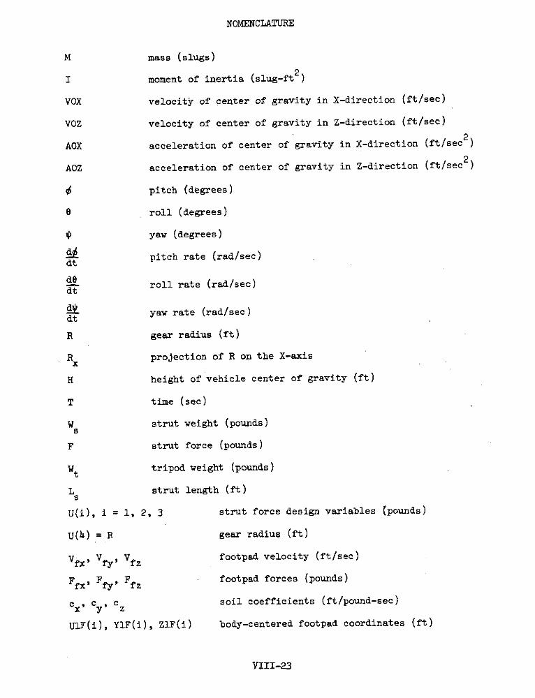
NOMENCLATURE
M mass (slugs)
I moment of inertia (slug-ft )
VOX velocity of center of gravity in X-direction (ft/sec)
VOZ velocity of center of gravity in Z-direction (ft/sec)
AOX acceleration of center of gravity in X-direction (ft/sec2)
AOZ acceleration of center of gravity in Z-direction (ft/sec2 )
pitch (degrees)
8 roll (degrees)
yaw (degrees)
pitch rate (rad/sec)dt
de roll rate (rad/sec)dt
dt yaw rate (rad/sec)
R gear radius (ft)
Rx projection of R on the X-axis
H height of vehicle center of gravity (ft)
T time (sec)
W strut weight (pounds)S
F strut force (pounds)
Wt tripod weight (pounds)
L strut length (ft)
U(i), i = 1, 2, 3 strut force design variables (pounds)
U(h) = R gear radius (ft)
V fx Vfy, Vfz footpad velocity (ft/sec)
Ffx , Ffy, Ffz footpad forces (pounds)
cx, cy c soil coefficients (ft/pound-sec)
UlF(i), YiF(i), ZLF(i) body-centered footpad coordinates (ft)
VIII-23

REFERENCES
1. Bendix - "Manned Flying System Landing Gear Study", Final Report,Bendix Products Aerospace Division, June 1966, Chapter 2.
2. Faculty Systems Engineering Institute: "Lunar Logistics Vehicle",NASA-ASEE, September 1969.
3. Lockheed - "Improved Lunar Cargo and Personnel Delivery Systems",Final Report, Lockheed Missiles and Space Company, June 1968.
4. Blanchard, Ulysse J., "Full-Scale Dynamic Landing-Impact Investi-gation of a Prototype Lunar Module Landing Gear", NASA TN D-5029,Langley Research Center, March 1969.
5. Blanchard, Ulysse J., "Evaluation of a Full-Scale Lunar-GravitySimulator by Comparison of the Landing-Impact Tests of a Full-Scale and 1/6-Scale Model", NASA TN D-4474, Langley ResearchCenter, June 1968.
6. Bendix - "An Approximate Solution of Lunar Vehicle Landing Stabi-lity", Midterm Report, Lunar Landing Dynamics Systems Investigation,Bendix Products Aerospace Division, June 1964.
7. Walton, W. C. Jr., R. W. Herr and H. W. Leonard, "Studies of Touch-down Stability for Lunar Landing Vehicles", Journal of Spacecraft,Vol. 1, No. 5, September 1964.
8. Black, R. J, "Quadrupal Landing Gear Systems for Spacecraft",Journal of Spacecraft, Vol. 1, No. 2, March 1964.
9. Admire, John and Alden Mackey, "Dynamic Analysis of a Multi-LeggedLunar Landing Vehicle to Determine Structural Loads During Touchdown",NASA TN D-2582, Huntsville, January 1965.
10. Walton, W. C. Jr., and Barbara J. Durling, "A Procedure for Computingthe Motion of a Lunar-Landing Vehicle During the Landing Impact",NASA TN D-4216, Langley Research Center, 1967.
11. Fox, Richard, "Optimization Methods for Engineering Design", Reading,Massachusetts, Addison-Wesley Publishing Company, 1971.
12. Black, R. J., "General Features of Landing Gear Systems for WidelyDifferent Design Specifications", Midterm Report, Lunar LandingDynamics Systems Investigation, Bendix Products Aerospace Division,June 1964.
13. Mantus, M., "Landing Dynamics of the Lunar Module", Grumman AircraftEngineering Corporation, June 15, 1967.
VIII-24

14. Bartel, D. L., E. J. Haug and K. Rim, "The Optimum Design ofSpatial Frames Using the Method of Constrained Steepest Descentwith State Equations", Journal of Engineering for Industry, Trans.ASME, Series B, Vol. 93, 1971.
15. Goldstein, Herbert, Classical Mechanics, Reading, Massachusetts,Addison-Wesley Publishing Company, c. 1950.
16. Deitrick, R. F., C. D. Conaway, L. W. Gammell and R. H. Jones,"Structures and Mechanical Environment", Surveyor 1 Flight Per-formance Final Report, SSD 68223, Vol. 3, Section 5.11.2,Hughes Aircraft Company, El Segundo, California, 1966.
17. Bendix - "Manned Flying System Landing Gear Study", Final Report,Bendix Products Aerospace Division, June 1966, Chapter 9.
18. Rojeski, Peter J., "A Systems Analysis Approach to Landing GearDesign", Ph.D. Thesis, Cornell University, Ithaca, N.Y., 1972.
VIII-25

Y
FORWARDDIRECTION X
\ THREE GEAR-INVERTED TRIFOD'
LANDING GEAR
Figure VIII-1
BALL JOINT-
ENERGY ABSORBER TPRIMARY STRUT
HSECONDARY STRUTS
FORWARD GEAR(S) BALL JOINT
Rx-
VIII-26

J=1
K=3 K=1
K= 2
J= 2
LUNAR LANDING VEHICLE:-
LANDING GEAR DESIGN
APPROXIMATE SCALE
1 IN. = 6 FT.
Figure VIII-2
10°
VIII-27

HARDPOINTS
SECONDARY PRIMARY STRUTSTRUT
SECONDARY STRUTSECONDARY ?- HARDPOINT
STRUTINVERTED TRIPOD DESIGN
PRIARY HARDPOINTSTRUT
SECONDARY STRUT
Figure VIII-3
CANTILEVER DESIGN
BRAKE BLOCK
GUIDE DISCLOWER TUBE
UPPER TEFLON RING TEFLON RINGTUBE
NASA FRICTION SHOCK ABSORBER CONCEPT
Figure VIII-4
VIII-28

L(1-COS6)
H /
STABILITY MARGIN PARAMETERS:i
Figure VIII-5

36
U(1) = 900034 AOX = -33
U(1) = 13,50032 AOX = -51
30
t 28
4 26 U() 7500
U(1) - 6000
24 Figure VIII-6
STABILITY MARGIN CURVES U(1) 3000U(2) = 8000
VOX = 4.022 VOZ = -2.0
to'0 0.2 0.4 0.6 0.8 1.0 1.2
TIME (SECONDS)
VIII-30