ARTICLE IN PRESS

0032-0633/$ - se

doi:10.1016/j.ps

�CorrespondE-mail addr

Planetary and Space Science 57 (2009) 201–215

www.elsevier.com/locate/pss

Collisional evolution of Trans-Neptunian populations:Effects of fragmentation physics and estimates of the

abundances of gravitational aggregates

Paula G. Benavidez, Adriano Campo Bagatin�

Departamento de Fısica, Ingenierıa de Sistemas y Teorıa de la Senal, Universidad de Alicante, P.O. Box 99, 03080 Alicante, Spain

Received 19 February 2008; received in revised form 5 September 2008; accepted 9 September 2008

Available online 26 September 2008

Abstract

The Trans-Neptunian region is yet another example of a collisional system of small bodies in the Solar System. In the last decade the

number of TNOs with reliable orbital elements is steadily increasing and even if it is still premature to compare models with observations,

we can start to have some idea of the orbital structure and magnitude distribution, so that some loose constraints may be set on the

critical parameters that affect collisional evolution. With this aim we have developed a model for the collisional evolution of the Trans-

Neptunian region by dividing it into three main different populations, corresponding to the dynamical classification proposed by

Gladman et al. [2001.The structure of the Kuiper Belt: size distribution and radial extent. Astrophys. J. 122, 1051] (Resonant region,

Classical Belt and Scattered Disk). A multi-zone collisional model is developed, in which each zone can collisionally interact with each

other. The model takes into account the known physics of the fragmentation of icy/rocky bodies at the typical relative velocities of

TNOs, according to velocity distributions corresponding to each evolving zone. The dependence of the evolution of the considered

populations on physically critical collisional parameters is investigated and the corresponding results are presented, including estimates

of the abundance of gravitational aggregates in the studied populations.

r 2008 Elsevier Ltd. All rights reserved.

Keywords: Trans-Neptunian objects; Collisional evolution; Fragmentation

1. Introduction

The origin of comets had been a puzzle for quite a longtime, until Oort (1950) suggested that the Solar System issurrounded by a cloud of comet-like objects scattered fromthe giant planet region during its formation. At present theOort cloud is identified as the source of long-periodComets.

In a similar way, the origin of short-period comets washypothesised independently by Edgeworth and Kuiperaround 1950. Fernandez (1980) showed analytically thatthere should actually be a reservoir of icy planetesimals in aflat region just beyond Neptune (the so-called Trans-Neptunian region, often referred to as the Edgeworth–

e front matter r 2008 Elsevier Ltd. All rights reserved.

s.2008.09.007

ing author. Tel.: +34619979012; fax: +34965909580.

ess: acb@ua.es (A. Campo Bagatin).

Kuiper Belt (EKB)), and suggested that should be thesource of short-period comets. The first Trans-Neptunianobject (TNO) was finally first observed in 1992 (Jewitt andLuu, 1993). The continuous discovery of TNOs since thenand further dynamical studies have shown that the EKB isa region extending outwards from the orbit of Neptune(at 30 AU) up to 50 AU and beyond. The studies of thephysical and dynamical properties of the TNOs isproviding important clues to understand the structure ofthe EKB, the origin of the TNOs and their formationprocesses. Even more important, these studies are funda-mental to understand the early stages of the formation ofthe Solar System.The discovery rate of TNOs has been steadily increasing

since 1992, due to a number of different surveys, to reachover �1000 TNOs. In particular, the Canadian FranceEcliptic Plane Survey (CFEPS)—in which the authors are

ARTICLE IN PRESSP.G. Benavidez, A. Campo Bagatin / Planetary and Space Science 57 (2009) 201–215202

involved—is performing a non-biased survey of the eclipticin search for TNOs and is setting up an orbitally well-characterised sample. This sample includes of order 150TNOs that have been observed at least at three oppositionsand thus have well-determined orbits. More than 200 otherbodies have been observed at two oppositions, so that theirorbital elements still have major uncertainty (Jones et al.,2006).

From the orbital distribution of the bodies with ‘‘good’’orbits, the EKB appears to contain at least threepopulations: TNOs trapped in Neptune’s 2:3 mean motionresonance (Plutinos) as well as other resonances; objectswith non-resonant orbits beyond 42 AU (the Classical

Belt); and objects with highly eccentric orbits that maypermit intermittent close approaches with Neptune (thescattered disk (SD)) (Duncan and Levison, 1997; Gladmanet al., 2001). Recently, a new dynamical class has beendetermined, the Extended SD (Gladman et al., 2001),whose objects have orbits similar to the SD, but with largerperihelia distances (larger than �40 AU), thus excludingstrong interactions with Neptune. However, due to thelimited number of observed TNOs, several aspects of theEKB are still largely undetermined. Among them, particu-larly important are the relative number of members ofthese populations, the eccentricity and inclination ‘‘excita-tion’’ (Petit et al., 1999), the radial extension of the classicalbelt (Gladman et al., 1998), the ratio between the numberof bodies in the 1:2 and in the 2:3 resonance (Jewitt et al.,1998).

Many crucial questions are still waiting for answersabout the TNO region: (i) How much mass was there in theTrans-Neptunian region at the very end of the planetformation process? (ii) How much of that mass was ejecteddue to dynamical interactions and how much due tocollisional erosion? (iii) What is—if any—the transition sizebetween populations of objects in a collisionally stationarystate and mostly pristine bodies? (iv) What is theabundance of objects gravitationally reaccumulated as aconsequence of catastrophic impacts? As astronomicalobservations increase in number and quality, numericalmodels may be compared to actual populations and shallhelp constraining some of the physical parameters thatcharacterize the response to collisions and/or the condi-tions in which the evolution took place.

The study of the collisional evolution of TNOs mayprovide clues to the understanding of the formation of thatregion. The behaviour of populations of planetesimals,asteroids or cometary bodies interacting collisionally isgenerally very complex. Both collisional properties andinitial conditions for the evolution have to be suitablyparametrised. A number of models have been proposed inthe past decade tackling this issue from different theoreticaland numerical approaches (e.g., Davis and Farinella, 1997;Kenyon and Bromley, 2004; Krivov et al., 2005; Pan andSari, 2005; Charnoz and Morbidelli, 2003, 2007).

A model for the collisional evolution of Trans-Neptu-nian populations of objects has been developed in this

work. In this paper the authors’ goal is to analyse thedependence of the collisional evolution on the criticalphysical parameters that govern fragmentation. In aforthcoming paper the dependence on the boundaryconditions for evolution, such as the different possibilitiesfor initial total available mass and its distribution, and theeffect of the migration of Neptune will be presented. Themodel is described (Section 2), and the analysis of theresults for the dependence of the collisional evolution onthe crucial parameters that characterise fragmentation andfor the estimated abundances for gravitational aggregates(GAs) (Section 3) is presented. Finally (Section 4), the mainconclusions of the study are summarised.

2. The model

In order to classify the very wide size range of objects inthe EKB, the size range of objects has been divided into aseries of logarithmic bins such that contiguous bins containobjects with masses differing by a factor of two, from thebin containing the largest objects—centred at 3000 km—down to 35 cm. The whole TNO region itself has beendivided into three dynamical zones, namely the Plutinos(Zone 1), the Classical Belt (Zone 2) and the SD (Zone 3).Each zone is characterised by a given semi-major axesrange for the orbits of objects and a typical eccentricity andinclination.As usual for the simulation of the collisional evolution of

small bodies populations, it is necessary to model both thecollisional processes and the evolution with time of thenumber of objects belonging to any size bin. In this case,we had to take care of the evolution of the three dynamicalzones altogether. Two main numerical codes have beenthen developed. The fragmentation code that performs thecollisional outcome of any impact between objects belong-ing to any couple of size bins is based on the fragmentationand reaccumulation models from Petit and Farinella(1993). A number of improvements have been introduced,based on recent available experimental data and onnumerical and theoretical studies. We have also implemen-ted the possibility to quantify and keep memory of theamount of reaccumulation that may occur after collisions.Contrarily to previous models dealing with the collisionalevolution of TNOs, the fact that relative velocities ofimpacts are widely dispersed has been taken into accountboth in the fragmentation and the evolution model.Both models contain 3–4 key parameters, each of them

may take some 2–4 sample values inside their range ofvariation. It is straightforward to see that the number ofpossible combinations quickly increases to hundreds. Forthis reason, we decided to sort our study out by dividing itinto two main parts. Firstly, we fix boundary conditionsand vary the critical parameters that determine fragmenta-tion conditions and fragments production, in order toinvestigate what their effects are on the overall sizedistribution of the three dynamical zones. The results ofthis part are reported in this work. Secondly, we fix the

ARTICLE IN PRESSP.G. Benavidez, A. Campo Bagatin / Planetary and Space Science 57 (2009) 201–215 203

parameters of collisional physics and let boundary condi-tions vary. The results corresponding to this part will bepresented in the near future.

In this way, we can study separately the influence offragmentation physics and boundary conditions on theoverall final mass of the belt and size distribution in eachdynamical zone considered.

2.1. Collisions

The basic idea of the fragmentation algorithm is tocompare the relative kinetic energy per unit volume of anycouple of colliding objects to the strength S of the target.Applying a suitable criterion, the outcome of any possibleimpact is set to be either a fragmentation or the formationof a crater (Greenberg et al., 1978). Finally, a massspectrum for the produced fragments is worked out—basedon the extrapolation of experimental results—and theextent of reaccumulation is also calculated. Experimentsshow non-unique results as far as the mass distribution offragments is concerned. Some experiments exhibit a fractaldistribution (single power-law), some other a brokendistribution, with shallower slopes at the low mass end.Both break mass and slopes are not unambiguouslydetermined though. For this reason, we prefer to beconservative on this point and stick to a single slope power-law for such distributions. This part of the model is basedon the Petit and Farinella (1993) fragmentation model,with some improvements described below. The modelincludes the possibility to also consider the effects due tothe shallow dependence of the velocity of the fragmentsejected in a collision on their mass (Nakamura andFujiwara, 1991; Giblin, 1998) and is outlined here.

The relative kinetic energy in a collision between a targetof mass MT and a projectile of mass MP is

Erel ¼1

2

MT MP

MT þMPV2

rel, (1)

where V rel is the relative impact velocity. Assuming that theenergy is partitioned equally between the two collidingbodies, a fragmentation occurs if SorErel=ð2MÞ (where M

is the mass of the target or projectile). If the impactstrength is below this threshold, cratering occurs. In bothcases the size distribution of the created fragments iscalculated. The critical quantity that discriminates crater-ing from shattering is the mass fraction between the largestremnant (MLR) and the target (MT), which is given by

f LR ¼MLR

MT¼ 0:5

SMT

rðErel=2Þ

� �1:24(2)

in the case of shattering, f LRp0:5.As for the reaccumulation process, we have followed

Campo Bagatin et al. (2001) in adopting two differentmodels.

(a) A ‘‘mass–velocity’’ model (Petit and Farinella, 1993),that assumes that there is a weak power-law correlationbetween the mass and velocity of fragments ejected in a

catastrophic collision, according to experimental results.The general aspect of the relationship between mass M andvelocity V that we adopted in our nominal case is

V /M�r. (3)

The value of exponent r has been found to be about 16by

Nakamura and Fujiwara (1991), or to be in between 0 and16, with a mean value of 1

13(Giblin, 1998), with a

considerable dispersion of data around the proposedslopes. This is the value assumed in our numericalsimulations. Any fragment with velocity larger than theescape velocity V esc, derived from the gravitationalpotential of the two colliding bodies, will escape, whilethose slower than V esc will reaccumulate on the largestremnant. In this model, a given mass corresponds to asingle velocity.(b) A so-called ‘‘cumulative’’ model, in which no

correlation between mass and velocity of fragments isconsidered. In this case, the velocity distribution is thesame for all fragments and the fraction of mass with avelocity larger than V is

f ð4V Þ �Mð4V Þ

MT¼

V

Vmin

� ��k

, (4)

where k is a given exponent, larger than 2 (to allowfor conservation of energy), and generally assumed to bek � 9

4, and Vmin is a lower cutoff for the velocity of

fragments. By integrating over V, between Vmin and1, thetotal kinetic energy of the ejected fragments, Efr, isobtained. Hence:

Vmin ¼

ffiffiffiffiffiffiffiffiffiffiffiffiffiffiffiffiffiffiffiffik � 2

k

Efr

MT

s. (5)

The kinetic energy of the fragments is a given fraction ofthe impact kinetic energy deposited in the target Erel=2:

Efr ¼ f KE

Erel

2. (6)

This model assumes that—in each mass bin—there arefragments with velocity larger than V esc, which wouldescape. The fraction of such fragments is f ð4V escÞ, the restis reaccumulated on the largest remnant.Necessary improvements to this model were simply

updates of the experimental results for collisions onto icytargets (Ryan et al., 1999; Burchell et al., 2005) and of theavailable scaling laws (SLs) for fragmentation, includingthe ones proposed by Benz and Asphaug (1999) (BA SL, inwhat follows), derived from the results of their hydrocodenumerical experiments.Between the SLs proposed by many authors, we have

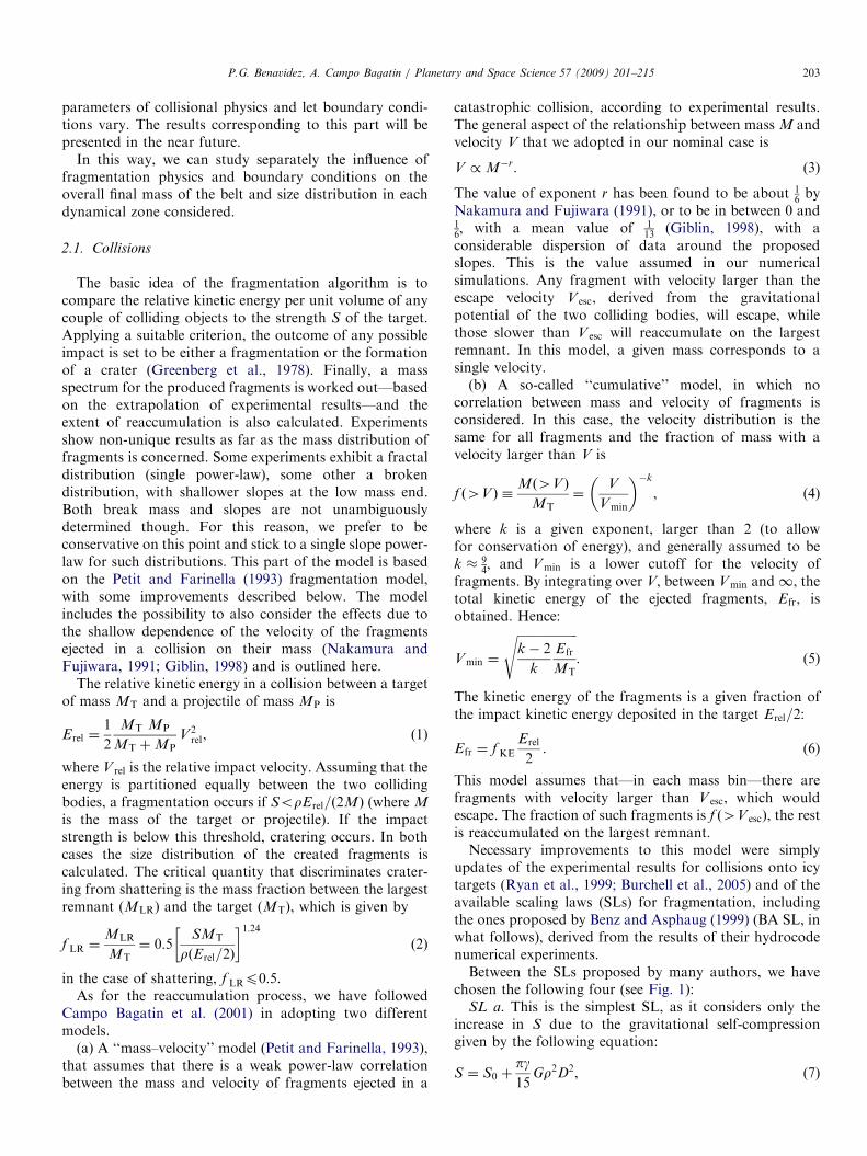
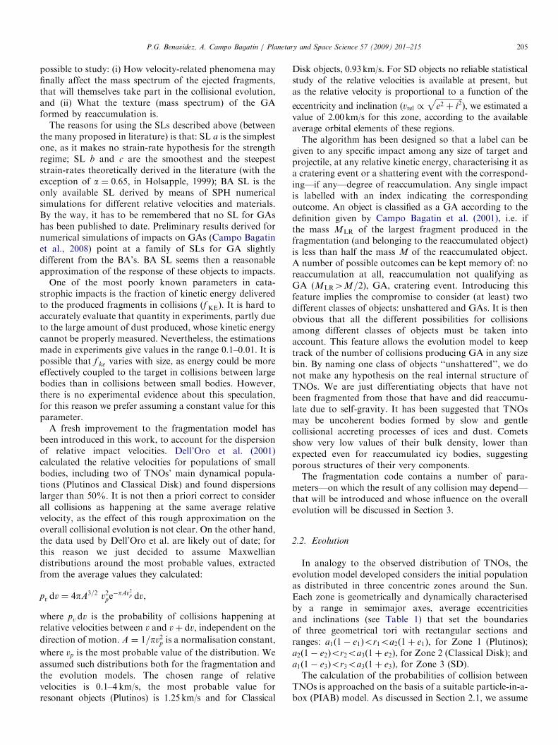
chosen the following four (see Fig. 1):SL a. This is the simplest SL, as it considers only the

increase in S due to the gravitational self-compressiongiven by the following equation:

S ¼ S0 þpg15

Gr2D2, (7)

ARTICLE IN PRESS

1012

1011

1010

109

108

107

106

105

104

1000

100

100.001 0.01 0.1 1

Size [km]10 100 1000 104

S [e

rg /

cm3 ]

S.L. a (So=105 erg / cm3)S.L. a (So=106 erg / cm3)S.L. a (So=107 erg / cm3)S.L. bS.L. cS.L. d

a

d

b

c

Fig. 1. Scaling laws for impact strength that have been used in the model.

The standard value S0 ¼ 106 erg=cm3 is used for scaling law a, b and c.

For scaling law d: Q0 ¼ 5:650� 107 erg=cm3;B ¼ 1:85 erg cm3=g2; a ¼

�0:43 and b ¼ 1:2. Each scaling law correspond to a relative velocity

V rel ¼ 1:25 km=s.

P.G. Benavidez, A. Campo Bagatin / Planetary and Space Science 57 (2009) 201–215204

where S0 is the material strength (the default value used is106 erg=cm3), g is the self-compression coefficient, G is thegravitational constant, r is the density, and D is the targetdiameter. In all our simulations, we have assumed g ¼ 100.

Two other SLs include self-compression and the effect ofstrain-rate suggested by Farinella et al. (1982), to include adecrease of the strength with increasing target size. Wedescribe this effect by the equation:

S0 ¼ SD

0:2m

� ��a, (8)

where S is given by Eq. (7), and a is an exponent.According to Housen and Holsapple (1990, 1999) andHolsapple (1994), different expressions have been proposedfor the scaling of this effect. Due to the lack of informationabout TNO materials, we assume two different exponents ain the power laws associated to them, resulting thus in thefollowing two SLs:

SL b. a ¼ 0:25.SL c. a ¼ 0:50.

SL d. Benz and Asphaug found the following family of SLsfor the specific energy (Q�D, per unit mass) necessary todisrupt different size targets, that is to shatter and disperseat least half of the mass of the parent body:

Q�D ¼ Q0

Rb

1 cm

� �a

þ BrRb

1 cm

� �b

, (9)

where Q0, a, b and B are values differing upon materialcomposition and relative velocity of impact. We considerthe proper values corresponding to ice, given by these

authors for such parameters. Suitable interpolationsbetween 0.5 and 3 km/s were performed according to thevelocity distributions for relative velocities described at theend of this subsection. For velocities between 3 and 4 km/sthe four parameters entering the SL were left constantassuming values estimated by Benz and Asphaug (1999) forvelocity of 3 km/s.We usually refer to the impact strength for shattering,

rather than to the disruption specific energy (that is, energyper unit target mass) Q�D, so, in order to compare them, weneed to pass to the shattering specific energy (criticalspecific energy for fragmentation), Q�S, and finally to thestrength S. This transformation was introduced by CampoBagatin et al. (2001) and is used in our numerical code.A remarkable difference between these two characteristicspecific energies is that Q�S allows to calculate the massspectrum of the fragments produced—based on laboratoryexperiments—regardless of the fact that some of them willbe finally reaccumulated. The connection between Q�D andQ�S can be worked out as follows.A relationship between Q�D and f KE must be defined. In

order to do so, a cumulative velocity distribution (Eq. (4))has to be considered. Since dispersal is defined byf ð4V escÞ41

2, from Eq. (4) we obtain that, for the critical

collision corresponding to Q�D, Vmin ¼ 2�1=k V esc. Let usrecall that Q�D is the minimum projectile energy requiredfor target dispersal, assuming that 1

2of the projectile energy

Erel is delivered to the target and that a fraction f KE of thisis partitioned into kinetic energy of fragments. Thus, forthe critical collision corresponding to Q�D we have

f KE ¼2Efr

MTQ�D¼

k

k � 22�2=k V2

esc

Q�D. (10)

The minimum energy to disperse a given target is definedas the sum of the energy needed to shatter the body and theenergy required to disperse the fragments (Durda andDermott, 1997):

Erel ¼ Q�DMT ¼Q�SMT

f SH

þ1

f KE

0:4112GM2

T

D. (11)

Here, f SH, the fraction of kinetic energy of the projectileused to shatter the target, is defined and assumed to be 1

2. InEq. (10), for consistency with Eq. (11), we have

V2esc ¼ 0:822

4GMT

D. (12)

This yields:

Q�S ¼ f SH Q�D �1

f KE

0:4112G MT

D

� �

¼ f SH Q�D 1�k � 2

k22=k 1

4

� �. (13)

Reaccumulation may be then calculated by comparingkinetic and potential gravitational energies of the fragments.This has the advantage to allow to insert or not, in thecalculation, any new experimentally found mass–velocitydependence, or simply a velocity field. In this way it is

ARTICLE IN PRESSP.G. Benavidez, A. Campo Bagatin / Planetary and Space Science 57 (2009) 201–215 205

possible to study: (i) How velocity-related phenomena mayfinally affect the mass spectrum of the ejected fragments,that will themselves take part in the collisional evolution,and (ii) What the texture (mass spectrum) of the GAformed by reaccumulation is.

The reasons for using the SLs described above (betweenthe many proposed in literature) is that: SL a is the simplestone, as it makes no strain-rate hypothesis for the strengthregime; SL b and c are the smoothest and the steepeststrain-rates theoretically derived in the literature (with theexception of a ¼ 0:65, in Holsapple, 1999); BA SL is theonly available SL derived by means of SPH numericalsimulations for different relative velocities and materials.By the way, it has to be remembered that no SL for GAshas been published to date. Preliminary results derived fornumerical simulations of impacts on GAs (Campo Bagatinet al., 2008) point at a family of SLs for GA slightlydifferent from the BA’s. BA SL seems then a reasonableapproximation of the response of these objects to impacts.

One of the most poorly known parameters in cata-strophic impacts is the fraction of kinetic energy deliveredto the produced fragments in collisions (f KE). It is hard toaccurately evaluate that quantity in experiments, partly dueto the large amount of dust produced, whose kinetic energycannot be properly measured. Nevertheless, the estimationsmade in experiments give values in the range 0.1–0.01. It ispossible that f ke varies with size, as energy could be moreeffectively coupled to the target in collisions between largebodies than in collisions between small bodies. However,there is no experimental evidence about this speculation,for this reason we prefer assuming a constant value for thisparameter.

A fresh improvement to the fragmentation model hasbeen introduced in this work, to account for the dispersionof relative impact velocities. Dell’Oro et al. (2001)calculated the relative velocities for populations of smallbodies, including two of TNOs’ main dynamical popula-tions (Plutinos and Classical Disk) and found dispersionslarger than 50%. It is not then a priori correct to considerall collisions as happening at the same average relativevelocity, as the effect of this rough approximation on theoverall collisional evolution is not clear. On the other hand,the data used by Dell’Oro et al. are likely out of date; forthis reason we just decided to assume Maxwelliandistributions around the most probable values, extractedfrom the average values they calculated:

pv dv ¼ 4pA3=2 v2pe�pAv2p dv,

where pv dv is the probability of collisions happening atrelative velocities between v and vþ dv, independent on the

direction of motion. A ¼ 1=pv2p is a normalisation constant,

where vp is the most probable value of the distribution. We

assumed such distributions both for the fragmentation andthe evolution models. The chosen range of relativevelocities is 0.1–4 km/s, the most probable value forresonant objects (Plutinos) is 1.25 km/s and for Classical

Disk objects, 0.93km/s. For SD objects no reliable statisticalstudy of the relative velocities is available at present, butas the relative velocity is proportional to a function of the

eccentricity and inclination (vrel /ffiffiffiffiffiffiffiffiffiffiffiffiffiffie2 þ i2

p), we estimated a

value of 2.00km/s for this zone, according to the availableaverage orbital elements of these regions.The algorithm has been designed so that a label can be

given to any specific impact among any size of target andprojectile, at any relative kinetic energy, characterising it asa cratering event or a shattering event with the correspond-ing—if any—degree of reaccumulation. Any single impactis labelled with an index indicating the correspondingoutcome. An object is classified as a GA according to thedefinition given by Campo Bagatin et al. (2001), i.e. ifthe mass MLR of the largest fragment produced in thefragmentation (and belonging to the reaccumulated object)is less than half the mass M of the reaccumulated object.A number of possible outcomes can be kept memory of: noreaccumulation at all, reaccumulation not qualifying asGA (MLR4M=2), GA, cratering event. Introducing thisfeature implies the compromise to consider (at least) twodifferent classes of objects: unshattered and GAs. It is thenobvious that all the different possibilities for collisionsamong different classes of objects must be taken intoaccount. This feature allows the evolution model to keeptrack of the number of collisions producing GA in any sizebin. By naming one class of objects ‘‘unshattered’’, we donot make any hypothesis on the real internal structure ofTNOs. We are just differentiating objects that have notbeen fragmented from those that have and did reaccumu-late due to self-gravity. It has been suggested that TNOsmay be uncoherent bodies formed by slow and gentlecollisional accreting processes of ices and dust. Cometsshow very low values of their bulk density, lower thanexpected even for reaccumulated icy bodies, suggestingporous structures of their very components.The fragmentation code contains a number of para-

meters—on which the result of any collision may depend—that will be introduced and whose influence on the overallevolution will be discussed in Section 3.

2.2. Evolution

In analogy to the observed distribution of TNOs, theevolution model developed considers the initial populationas distributed in three concentric zones around the Sun.Each zone is geometrically and dynamically characterisedby a range in semimajor axes, average eccentricitiesand inclinations (see Table 1) that set the boundariesof three geometrical tori with rectangular sections andranges: a1ð1� e1Þor1oa2ð1þ e1Þ, for Zone 1 (Plutinos);a2ð1� e2Þor2oa3ð1þ e2Þ, for Zone 2 (Classical Disk); anda1ð1� e3Þor3oa3ð1þ e3Þ, for Zone 3 (SD).The calculation of the probabilities of collision between

TNOs is approached on the basis of a suitable particle-in-a-box (PIAB) model. As discussed in Section 2.1, we assume

ARTICLE IN PRESS

Table 1

Average eccentricities (e) and inclinations (i) in the corresponding semi-

major axes ranges (a), for TNOs observed at least at three oppositions

(Minor Planet Center and CFEPS database. The authors—as members of

the CFEPS—have access to updated data from the survey)

Zone a ðAUÞ e se i (deg) si M0 (ME)

Zone 1 (Plutinos) 35240 0.18 0.08 9.9 7.3 9.69

Zone 2 (Classical) 40250 0.08 0.05 3.7 3.2 5.31

Zone 3 (Scattered disk) 35250 0.18 0.12 20.1 7.8 15.00

P.G. Benavidez, A. Campo Bagatin / Planetary and Space Science 57 (2009) 201–215206

a statistical distribution for relative velocities of impacts.This implies a different collisional outcome and a differentnumber of collisions in any given interval of time for anysingle value of the velocity distribution. For this reason, wedivided the relative velocity range into a series of discreteintervals (number may be chosen upon convenience,namely 20), each of which has an associated probability,and performed the calculation according to it. In this way,the number of collisions among Ni objects of size Di andNj objects of size Dj—in a given interval of time Dt

corresponding to a given interval of relative velocities vl

and inside a given zone—can be calculated. The variationper time step in the number of objects belonging to a givenbin k is then given by

DNðkÞ ¼Xn

i

Xi

j

Xm

l

½f ði; j; k; lÞ pðvlÞ si;j;l �

( )

�ðNðiÞ � dijÞ NðjÞ

1þ dij

Dt, (14)

where n and m are the total number of size and velocity bins,respectively. The projectile index j ranges from 1 to i, due tothe symmetrical nature of the f ði; j; k; lÞ matrix, which is theoutput of the modified (Petit and Farinella, 1993) fragmenta-tion algorithm; pðvlÞ, is the probability corresponding to thelth generic discrete interval of relative velocities centred

around vl and si;j;l ¼14

Pint ðDi þDjÞ2 f1þ ðV esc=vlÞ

2g,

being V esc ¼

ffiffiffiffiffiffiffiffiffiffiffiffiffiffiffiffiffi83prGR2

qthe escape velocity from the target

body (r is the density of bodies, G the gravitationalconstant), and Pint the intrinsic collision probability (whichis a function of the relative velocity and orbital elements for

each zone), its value ranges from 10�22 km2 yr�1 for the SD

to 5� 10�22 km2 yr�1 for Plutinos and Classical Disk.Finally, dij ¼ 1 if i ¼ j, and 0 otherwise.

As usual, in order to avoid undesired wavy effects due toan abrupt truncation of the size distribution at small sizes(Campo Bagatin et al., 1994), a number of the smallest sizeintervals (from 35 cm to 30m) have been used to produce alow-end ‘‘tail’’. Then the collisional evolution of these binsis estimated using a power-law extrapolation from the sizedistribution of the next 10 bins.

2.2.1. Interactions between dynamical zones

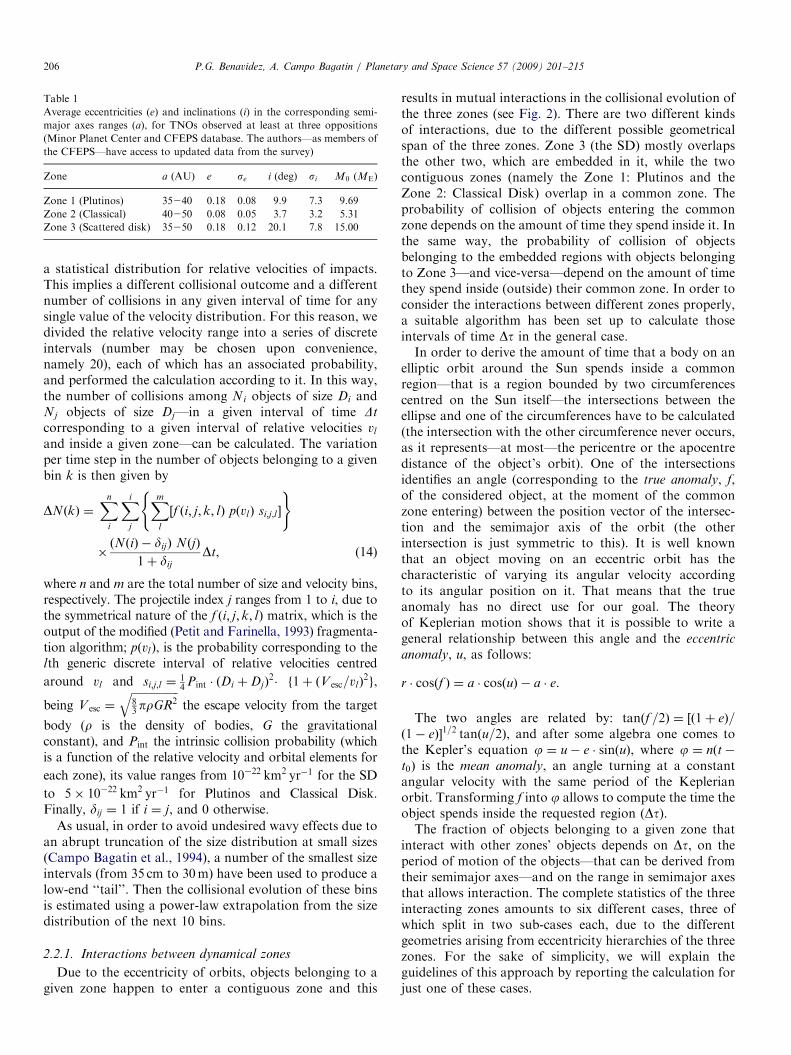
Due to the eccentricity of orbits, objects belonging to agiven zone happen to enter a contiguous zone and this

results in mutual interactions in the collisional evolution ofthe three zones (see Fig. 2). There are two different kindsof interactions, due to the different possible geometricalspan of the three zones. Zone 3 (the SD) mostly overlapsthe other two, which are embedded in it, while the twocontiguous zones (namely the Zone 1: Plutinos and theZone 2: Classical Disk) overlap in a common zone. Theprobability of collision of objects entering the commonzone depends on the amount of time they spend inside it. Inthe same way, the probability of collision of objectsbelonging to the embedded regions with objects belongingto Zone 3—and vice-versa—depend on the amount of timethey spend inside (outside) their common zone. In order toconsider the interactions between different zones properly,a suitable algorithm has been set up to calculate thoseintervals of time Dt in the general case.In order to derive the amount of time that a body on an

elliptic orbit around the Sun spends inside a commonregion—that is a region bounded by two circumferencescentred on the Sun itself—the intersections between theellipse and one of the circumferences have to be calculated(the intersection with the other circumference never occurs,as it represents—at most—the pericentre or the apocentredistance of the object’s orbit). One of the intersectionsidentifies an angle (corresponding to the true anomaly, f,of the considered object, at the moment of the commonzone entering) between the position vector of the intersec-tion and the semimajor axis of the orbit (the otherintersection is just symmetric to this). It is well knownthat an object moving on an eccentric orbit has thecharacteristic of varying its angular velocity accordingto its angular position on it. That means that the trueanomaly has no direct use for our goal. The theoryof Keplerian motion shows that it is possible to write ageneral relationship between this angle and the eccentric

anomaly, u, as follows:

r cosðf Þ ¼ a cosðuÞ � a e.

The two angles are related by: tanðf =2Þ ¼ ½ð1þ eÞ=ð1� eÞ�1=2 tanðu=2Þ, and after some algebra one comes tothe Kepler’s equation j ¼ u� e sinðuÞ, where j ¼ nðt�

t0Þ is the mean anomaly, an angle turning at a constantangular velocity with the same period of the Keplerianorbit. Transforming f into j allows to compute the time theobject spends inside the requested region (Dt).The fraction of objects belonging to a given zone that

interact with other zones’ objects depends on Dt, on theperiod of motion of the objects—that can be derived fromtheir semimajor axes—and on the range in semimajor axesthat allows interaction. The complete statistics of the threeinteracting zones amounts to six different cases, three ofwhich split in two sub-cases each, due to the differentgeometries arising from eccentricity hierarchies of the threezones. For the sake of simplicity, we will explain theguidelines of this approach by reporting the calculation forjust one of these cases.

ARTICLE IN PRESS

Fig. 2. Scheme of an overlapping region. The true anomaly, f, for a sample orbit of an object of Zone 1 entering Zone 2 is indicated.

P.G. Benavidez, A. Campo Bagatin / Planetary and Space Science 57 (2009) 201–215 207

Our sample case refers to the case of objects belonging toZone 2 (Classical Disk) that interact with objects from Zone1 (Plutinos) entering Zone 2, in the realistic case of e2oe1.

In this case, we have to calculate what is the effectivefraction of objects belonging to Zone 1 that reach Zone 2.For those objects, Dt12 (the interval of time per period theyspend in Zone 2) can be worked out as described above. Onthe other hand, the semimajor axes of Zone 1 objects thatmay actually enter Zone 2 are those given by the condition:a2ð1� e2Þoaoa2ð1þ e1Þ and the corresponding interval is

Da12 ¼

a2 �a2ð1� e2Þ

1þ e1ða2 � a1Þ

.

As a result, the fraction of objects belonging to Zone 1spending part of their orbital periods in the common regionwith Zone 2 is

x12 ¼ Da12 Dt12T12

� �

1 if i2Xi1;i2

i1if i2oi1;

8<:

where Dt12 ¼ T12 ð1� j12=pÞ, is the average time Zone 1objects spend inside Zone 2, j12 is the average valuefor the mean anomaly corresponding to objects in ellipticorbits intersecting the circular border of the commonregion. T12 is the orbital period of objects from Zone 1entering Zone 2.

In this way, starting from the intersections betweenobjects’ orbits and common zones, the fraction of time thataverage objects spend in common zones is calculated and

the fraction of objects of any zone that interact with otherzones is calculated accordingly.Finally, the number of objects of Zone 1 of a given size

bin h interacting with Zone 2 is: N12ðhÞ ¼ N1ðhÞ x12, andthis number has to be included in the NðiÞ or NðjÞ term inEq. (14).When collisions happen in a common region, among

objects coming from neighbouring zones, we assume thatthe fragments created are distributed into the correspond-ing bins and belong to the same zone as the largest parentobject. If the parent objects are equal sized and come fromdifferent zones, the fragments are equally distributedbetween the two zones.As described in Section 2.1, the fragmentation algorithm

labels collisions leading to the formation of GA. Thisallows to calculate, at any single time step, the amount ofnew GA created in any size bin—and in any dynamicalzone—for all collisional couples and any considered valueof the relative velocities. Interactions between differentzones and different kinds of objects (unshattered or GA)are rigorously taken into account, with no simplifyingassumption. Keeping memory of these quantities it ispossible to follow the evolution of the number of GA withtime, corresponding to each size bin and zone.

3. Results: dependence on collisional parameters

In order to study in detail the dependence of thecollisional evolution on the physical characteristics thatmostly influence the fragmentation model, we had to fix

ARTICLE IN PRESS

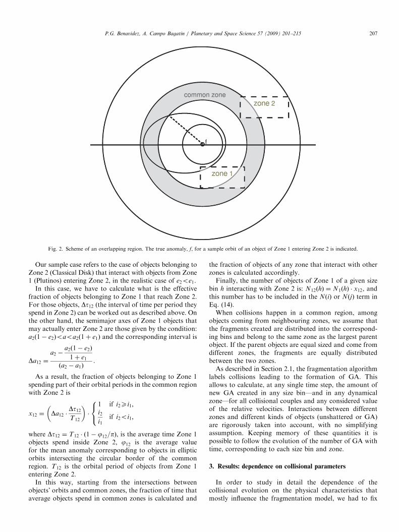
Fig. 3. Dependence of mass on time, for all adopted scaling laws for

strength. The black dot represents the present day estimated mass, which

is one order of magnitude smaller than the final mass obtained from our

simulations.

P.G. Benavidez, A. Campo Bagatin / Planetary and Space Science 57 (2009) 201–215208

boundary conditions first. By analysing the results of thevery many different initial conditions, we decided thatthe following one was the most likely set. The total mass ofthe primitive belt is fixed to 30ME (Earth masses) (Sternand Colwell, 1997): a half of the initial mass corresponds toZone 3 (SD), and the rest is distributed between Zone 1(Plutinos) and 2 (Classical Disk) proportionally to theirvolumes. We assume that the evolution takes place—forthe three populations of bodies—inside the volumedelimited by the same average values for the semimajoraxes, eccentricities and inclinations, observed at present foreach dynamical zone (see Table 1). No migration ofNeptune, nor excitation of the belt is considered.

We mimic the initial distribution of bodies by means oftwo power-law (Pareto) distributions joined at an initialtransition size (Dtri) at 100 km.

dNðDÞ / D�b1 dD if DpDtri

dNðDÞ / D�b2 dD if D4Dtri (15)

with (b1; b2Þ ¼ ð4; 4:5Þ. All simulations show an excess offinal mass with respect to current estimates, mostly due tothe fact that no dynamical effect is taken into account inthe model. If those effects are able to lower down the massaccordingly, then the chosen initial conditions set is onethat best preserves one of the available observables: thenumber of known bodies larger than 2000 km.

Once boundary conditions were stated, the study of therange of physical parameters was carried on. The density ofthe material of which TNOs are supposed to be made ofwas also fixed to the value 1:0 g=cm3, that is a typical valuefor ices.

Where not explicitly stated, we assume SL a, b and c forunshattered objects and d for GAs. In the cases where wecompare the effects of different SLs, we assume a same SLfor all bodies, and consider GAs to have a value of f KE ¼

0:005 while keeping the standard value of 0.05 forunshattered objects.

In this way we reduced the number of free parameters tofour: the SL for the strength, the value of the materialstrength (S0) itself, the response of GAs to collisions, andthe fraction of the impact kinetic energy delivered tofragments (f KE).

3.1. Comparing the effects of different SLs

One of the main questions about the present Trans-Neptunian population is about the lack of mass withrespect to the initial mass. At present, mass is estimated tobe 0.02 to 0:2ME (Jewitt and Luu, 2000; Bernstein et al.,2004).

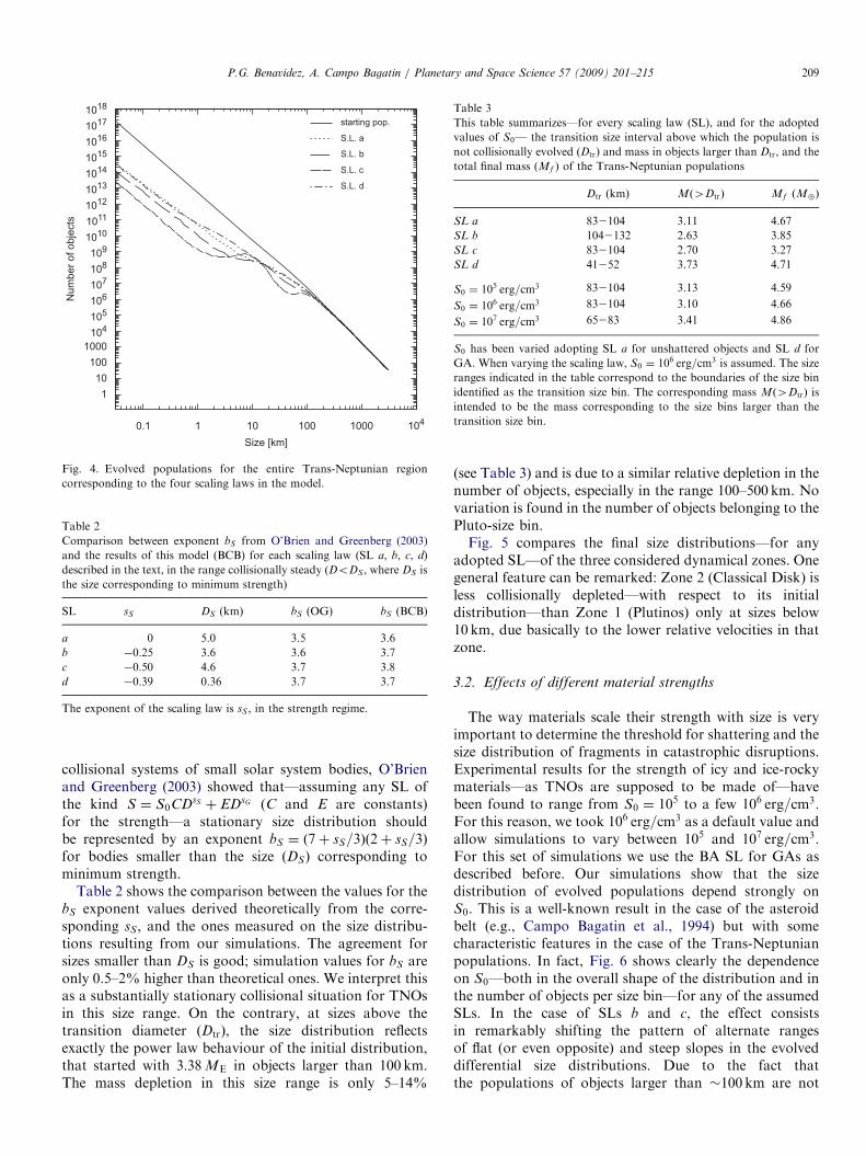
Fig. 3 shows the time evolution of the total mass of thebelt due to collisional grinding. Evolution starts with30ME and quickly erodes 25–50% of the initial mass inabout 0.1Myr, depending on SL. Between 10Myr and4500Myr the mass follows a logarithmic decrease, down to3.3 to 4:9ME, described approximately by MðtÞ ¼M1 � b

logðt=t1Þ, where M is the mass at t1�100 Myr and b ’ 0:9.Present day estimated mass is one order of magnitudesmaller than the final mass in our simulations. This showsthat the collisional evolution on its own is not effectiveenough to reproduce what we can infer from observations.Even if more mass than currently estimated may be presentin the Trans-Neptunian region, other processes—likedynamical effects due to resonances with a migratingNeptune, or interactions with a passing star—should betaken into account at the same time than the collisionalgrinding with the goal to reproduce available data (e.g.,Charnoz and Morbidelli, 2003, 2007).As expected, SL b—and especially c—are the ones that

result in a lower amount of mass at the end of thecollisional evolution. This trend is also clear in Fig. 4,where the differential size distribution of objects is shown.Erosion acts more efficiently at sizes corresponding to theminimum of the strength, triggering a wavy behaviour(Durda and Dermott, 1997; Campo Bagatin et al., 1994) atlarger sizes. This pattern does not show up in the case ofSLs a (constant strength below gravity regime) and d (BASL), due to the corresponding high values for strength atthe same size range (see Fig. 1). The behaviour of the sizedistribution in these cases is quite similar, only differing(about 50%) in the number of objects in the 1–10 km range.It is well known that the size distribution of a collisional

cascade sticks to the power law distribution shown byDohnanyi (1969) (bs ¼ �3:5) only in the very specialcase of collisional response independent on target size(assuming no abrupt cutoff is present in the small end ofthe distribution). As this is not the case in the real

ARTICLE IN PRESS

1018

1017

1016

101010111012101310141015

109

108

107

106

105

104

1001000

101

0.1 1Size [km]10 100 1000 104

Num

ber o

f obj

ects

starting pop.

S.L. a

S.L. b

S.L. c

S.L. d

Fig. 4. Evolved populations for the entire Trans-Neptunian region

corresponding to the four scaling laws in the model.

Table 2

Comparison between exponent bS from O’Brien and Greenberg (2003)

and the results of this model (BCB) for each scaling law (SL a, b, c, d)

described in the text, in the range collisionally steady (DoDS , where DS is

the size corresponding to minimum strength)

SL sS DS (km) bS (OG) bS (BCB)

a 0 5.0 3.5 3.6

b �0:25 3.6 3.6 3.7

c �0:50 4.6 3.7 3.8

d �0:39 0.36 3.7 3.7

The exponent of the scaling law is sS , in the strength regime.

Table 3

This table summarizes—for every scaling law (SL), and for the adopted

values of S0— the transition size interval above which the population is

not collisionally evolved (Dtr) and mass in objects larger than Dtr, and the

total final mass (Mf ) of the Trans-Neptunian populations

Dtr ðkmÞ Mð4DtrÞ Mf ðMÞ

SL a 832104 3.11 4.67

SL b 1042132 2.63 3.85

SL c 832104 2.70 3.27

SL d 41252 3.73 4.71

S0 ¼ 105 erg=cm3 832104 3.13 4.59

S0 ¼ 106 erg=cm3 832104 3.10 4.66

S0 ¼ 107 erg=cm3 65283 3.41 4.86

S0 has been varied adopting SL a for unshattered objects and SL d for

GA. When varying the scaling law, S0 ¼ 106 erg=cm3 is assumed. The size

ranges indicated in the table correspond to the boundaries of the size bin

identified as the transition size bin. The corresponding mass Mð4DtrÞ is

intended to be the mass corresponding to the size bins larger than the

transition size bin.

P.G. Benavidez, A. Campo Bagatin / Planetary and Space Science 57 (2009) 201–215 209

collisional systems of small solar system bodies, O’Brienand Greenberg (2003) showed that—assuming any SL ofthe kind S ¼ S0CDsS þ EDsG (C and E are constants)for the strength—a stationary size distribution shouldbe represented by an exponent bS ¼ ð7þ sS=3Þð2þ sS=3Þfor bodies smaller than the size (DS) corresponding tominimum strength.

Table 2 shows the comparison between the values for thebS exponent values derived theoretically from the corre-sponding sS, and the ones measured on the size distribu-tions resulting from our simulations. The agreement forsizes smaller than DS is good; simulation values for bS areonly 0.5–2% higher than theoretical ones. We interpret thisas a substantially stationary collisional situation for TNOsin this size range. On the contrary, at sizes above thetransition diameter (DtrÞ, the size distribution reflectsexactly the power law behaviour of the initial distribution,that started with 3:38ME in objects larger than 100 km.The mass depletion in this size range is only 5–14%

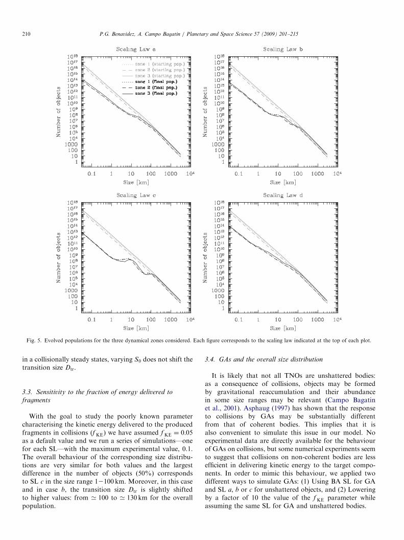
(see Table 3) and is due to a similar relative depletion in thenumber of objects, especially in the range 100–500 km. Novariation is found in the number of objects belonging to thePluto-size bin.Fig. 5 compares the final size distributions—for any

adopted SL—of the three considered dynamical zones. Onegeneral feature can be remarked: Zone 2 (Classical Disk) isless collisionally depleted—with respect to its initialdistribution—than Zone 1 (Plutinos) only at sizes below10 km, due basically to the lower relative velocities in thatzone.

3.2. Effects of different material strengths

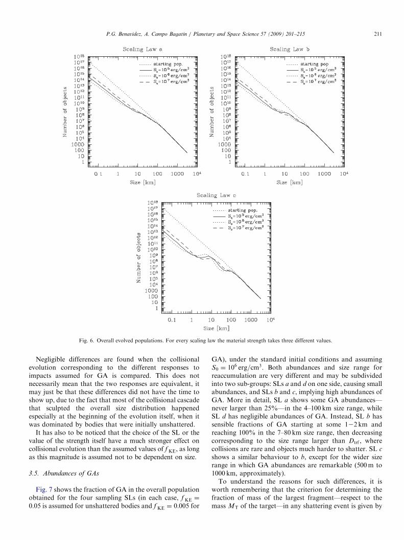
The way materials scale their strength with size is veryimportant to determine the threshold for shattering and thesize distribution of fragments in catastrophic disruptions.Experimental results for the strength of icy and ice-rockymaterials—as TNOs are supposed to be made of—havebeen found to range from S0 ¼ 105 to a few 106 erg=cm3.For this reason, we took 106 erg=cm3 as a default value andallow simulations to vary between 105 and 107 erg=cm3.For this set of simulations we use the BA SL for GAs asdescribed before. Our simulations show that the sizedistribution of evolved populations depend strongly onS0. This is a well-known result in the case of the asteroidbelt (e.g., Campo Bagatin et al., 1994) but with somecharacteristic features in the case of the Trans-Neptunianpopulations. In fact, Fig. 6 shows clearly the dependenceon S0—both in the overall shape of the distribution and inthe number of objects per size bin—for any of the assumedSLs. In the case of SLs b and c, the effect consistsin remarkably shifting the pattern of alternate rangesof flat (or even opposite) and steep slopes in the evolveddifferential size distributions. Due to the fact thatthe populations of objects larger than �100 km are not

ARTICLE IN PRESS

Fig. 5. Evolved populations for the three dynamical zones considered. Each figure corresponds to the scaling law indicated at the top of each plot.

P.G. Benavidez, A. Campo Bagatin / Planetary and Space Science 57 (2009) 201–215210

in a collisionally steady states, varying S0 does not shift thetransition size Dtr.

3.3. Sensitivity to the fraction of energy delivered to

fragments

With the goal to study the poorly known parametercharacterising the kinetic energy delivered to the producedfragments in collisions (f KE) we have assumed f KE ¼ 0:05as a default value and we run a series of simulations—onefor each SL—with the maximum experimental value, 0.1.The overall behaviour of the corresponding size distribu-tions are very similar for both values and the largestdifference in the number of objects (50%) correspondsto SL c in the size range 12100 km. Moreover, in this caseand in case b, the transition size Dtr is slightly shiftedto higher values: from ’ 100 to ’ 130 km for the overallpopulation.

3.4. GAs and the overall size distribution

It is likely that not all TNOs are unshattered bodies:as a consequence of collisions, objects may be formedby gravitational reaccumulation and their abundancein some size ranges may be relevant (Campo Bagatinet al., 2001). Asphaug (1997) has shown that the responseto collisions by GAs may be substantially differentfrom that of coherent bodies. This implies that it isalso convenient to simulate this issue in our model. Noexperimental data are directly available for the behaviourof GAs on collisions, but some numerical experiments seemto suggest that collisions on non-coherent bodies are lessefficient in delivering kinetic energy to the target compo-nents. In order to mimic this behaviour, we applied twodifferent ways to simulate GAs: (1) Using BA SL for GAand SL a, b or c for unshattered objects, and (2) Loweringby a factor of 10 the value of the f KE parameter whileassuming the same SL for GA and unshattered bodies.

ARTICLE IN PRESS

Fig. 6. Overall evolved populations. For every scaling law the material strength takes three different values.

P.G. Benavidez, A. Campo Bagatin / Planetary and Space Science 57 (2009) 201–215 211

Negligible differences are found when the collisionalevolution corresponding to the different responses toimpacts assumed for GA is compared. This does notnecessarily mean that the two responses are equivalent, itmay just be that these differences did not have the time toshow up, due to the fact that most of the collisional cascadethat sculpted the overall size distribution happenedespecially at the beginning of the evolution itself, when itwas dominated by bodies that were initially unshattered.

It has also to be noticed that the choice of the SL or thevalue of the strength itself have a much stronger effect oncollisional evolution than the assumed values of f KE, as longas this magnitude is assumed not to be dependent on size.

3.5. Abundances of GAs

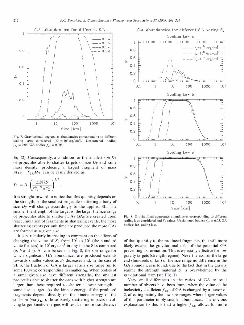
Fig. 7 shows the fraction of GA in the overall populationobtained for the four sampling SLs (in each case, f KE ¼

0:05 is assumed for unshattered bodies and f KE ¼ 0:005 for

GA), under the standard initial conditions and assumingS0 ¼ 106 erg=cm3. Both abundances and size range forreaccumulation are very different and may be subdividedinto two sub-groups: SLs a and d on one side, causing smallabundances, and SLs b and c, implying high abundances ofGA. More in detail, SL a shows some GA abundances—never larger than 25%—in the 4–100 km size range, whileSL d has negligible abundances of GA. Instead, SL b hassensible fractions of GA starting at some 122 km andreaching 100% in the 7–80 km size range, then decreasingcorresponding to the size range larger than Dtrf , wherecollisions are rare and objects much harder to shatter. SL c

shows a similar behaviour to b, except for the wider sizerange in which GA abundances are remarkable (500m to1000 km, approximately).To understand the reasons for such differences, it is

worth remembering that the criterion for determining thefraction of mass of the largest fragment—respect to themass MT of the target—in any shattering event is given by

ARTICLE IN PRESS

Fig. 7. Gravitational aggregates abundancies corresponding to different

scaling laws considered (S0 ¼ 106 erg=cm3). Unshattered bodies:

f ke ¼ 0:05, GA bodies: f ke ¼ 0:005.

Fig. 8. Gravitational aggregates abundancies corresponding to different

scaling laws considered and S0 values. Unshattered bodies: f ke ¼ 0:05, GA

bodies: BA scaling law.

P.G. Benavidez, A. Campo Bagatin / Planetary and Space Science 57 (2009) 201–215212

Eq. (2). Consequently, a condition for the smallest size DP

of projectiles able to shatter targets of size DT and samemass density, producing a largest fragment of massMLR ¼ f LRMT, can be easily derived as

DP ¼ DT2:287S

f1=1:24LR rV2

rel

!1=3

.

It is straightforward to notice that this quantity depends onthe strength, so the smallest projectile shattering a body ofsize DT will change accordingly to the applied SL. Thesmaller the strength of the target is, the larger the size rangeof projectiles able to shatter it. As GAs are created uponreaccumulation of fragments in shattering events, the moreshattering events per unit time are produced the more GAsare formed at a given size.

It is particularly interesting to comment on the effects ofchanging the value of S0 from 105 to 106 (the standardvalue for ices) to 107 erg=cm3 in any of the SLs compared(a, b and c). As can be seen in Fig. 8, the size range forwhich significant GA abundances are produced extendstowards smaller values as S0 decreases and, in the case ofSL a, the fraction of GA is larger at any size range (up tosome 100 km) corresponding to smaller S0. When bodies ofa same given size have different strengths, the smallestprojectiles able to shatter the ones with higher strength arelarger than those required to shatter a lower strength—same size—target. As the kinetic energy of the producedfragments depend directly on the kinetic energy of thecollision (via f KE), those barely shattering impacts invol-ving larger kinetic energies will result in more transference

of that quantity to the produced fragments, that will morelikely escape the gravitational field of the potential GApreventing its formation. This is especially effective for lowgravity targets (strength regime). Nevertheless, for the largeend (hundreds of km) of the size range no difference in theGA abundances is found, due to the fact that in the gravityregime the strength material S0 is overwhelmed by thegravitational term (see Fig. 1).Very small differences in the ratios of GA to total

number of objects have been found when the value of theinelasticity coefficient f KE of GA is changed by a factor of2, affecting mainly the low size ranges, where larger valuesof this parameter imply smaller abundances. The obviousexplanation to this is that a higher f KE allows for more

ARTICLE IN PRESSP.G. Benavidez, A. Campo Bagatin / Planetary and Space Science 57 (2009) 201–215 213

kinetic energy in fragments that are more likely to escape—especially from low mass bodies—than in the case of lowervalues.

Even smaller differences are found when comparing theabundances of GA that have been produced by (i) loweringf KE by an order of magnitude, or (ii) considered followingSL d for dispersion.

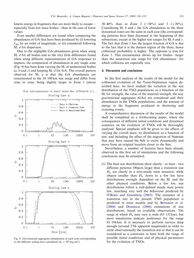
Due to the negligible GA abundances given when usingSL d for all bodies and to the very little differences foundwhen using different representations of GA responses toimpacts, the comparison of abundances in any single zone(Fig. 9) has been done varying the SL of unshattered bodies(a, b and c) and keeping SL d for GA. The overall patternobserved for SL a is that the GA abundances areconcentrated in the 10–100 km size range and differ fromzone to zone, being slightly larger in Zone 1 (about

Fig. 9. Gravitational aggregates abundancies in each zone corresponding

to the different scaling laws considered (S0 ¼ 106 erg=cm3).

30–40% than in Zone 2 (�30%) and 3 (o20%).Considering SL b and c the GA abundances in the threedynamical zones are the same in each case (the correspond-ing patterns have been discussed at the beginning of thissubsection), except at the higher size ranges for SL b and c.The fact that Zone 1 has the largest fraction of GA is dueto the fact that it is the densest region of the three, hencecollisional probability is higher. The opposite is true forZone 3. This circumstance shows up for bodies—largerthan the saturation size range for GA abundances—forwhich collisions are especially rare.

4. Discussion and conclusions

In this first analysis of the results of the model for thecollisional evolution of the Trans-Neptunian region de-scribed here, we have studied the variation in the sizedistribution of the TNO populations as a function of theSL for strength, the value of the material strength, the waygravitational aggregates (GAs) are considered and theirabundances in the TNOs populations, and the amount ofenergy in the fragments produced in shattering andcratering events.A comprehensive discussion of the results of the model

shall be completed in a forthcoming paper, where theconsequences of different initial conditions and dynamicalscenarios on the evolution of TNOs will be thoroughlyanalysed. Special emphasis will be given to the effects ofvarying the overall mass, its distribution as a function ofsize, and including the effect of the migration of Neptunethat may have caused the belt to excite dynamically andmove from an original location closer to the Sun.Nevertheless, a number of features have been already

observed in this first set of simulations and the followingconclusions may be attempted.

(1)

The final size distributions show clearly—at least—twodifferent patterns: Objects larger than a transition sizeDtr are clearly in a non-steady state situation, whileobjects smaller than Dtr down to a few km havedistributions strongly dependent on the SL and theother physical conditions. Below a few km, sizedistributions follow a well-defined steady state powerlaw, matching very well the behaviour predicted byO’Brien and Greenberg (2003). The existence of atransition size in the present TNO population ispredicted in most models and by Bernstein et al.(2004) and Donnison (2006) estimations of sizedistributions, based on available observations. Therange in which Dtr may vary is wide (65–132 km), butmost simulations indicate preference for the range83–104 km. It is necessary to perform surveys deepenough (around 27th apparent magnitude) in order tosettle observationally the transition size so that it can beconsidered as a constraint to limit both the range ofpossible initial conditions and of physical parametersfor the evolution of TNOs.

ARTICLE IN PRESSP.G. Benavidez, A. Campo Bagatin / Planetary and Space Science 57 (2009) 201–215214

(2)

The collisional evolution grinded down to cm-sizeparticles, and smaller, 94–98% of the original mass ofobjects smaller than Dtr. Instead, 80–93% of theoriginal mass contained in objects larger than Dtr

should still be part of the TNO populations. Thenumber of objects in this size range is approximatelythe same than at the beginning of the evolution. Thenumber of largest objects ð42000 kmÞ has not changed.This result clearly seems to point at confirming Davisand Farinella (1997) conclusion that objects over some100 km in size: (i) are not collisionally evolved, and (ii)may be mostly pristine.

(3)

The collisional evolution is very effective at its veryearly stages. Depending on different physical charac-teristics, 25–50% of the initial mass is eroded in the first100Myr. A logarithmic decrease of mass takes oversince a few Myr of evolution. The total final mass of theconsidered Trans-Neptunian region ranges from 3.3 to4:8ME: only about 12–18% of the original mass. Thisnumber is some 10 times larger than the actualestimated mass, indicating that dynamical mechanismsplayed a role in ejecting mass from that region (Ida etal., 2000; Levison and Morbidelli, 2003).

(4)

The different ways in which the disruption of GAs aremodelled do not seem to affect the overall results of thecollisional evolution. The fact that most of it occurredin the very early stages—when GAs where notabundant at all sizes—may be responsible for that.

(5)

To model in different ways how GA respond to impactsdoes not affect nor the overall collisional evolution ofTNOs, nor the abundance of estimated GA, within thelimits explored in this study. Nevertheless, the fractionof GA as a function of size is strongly dependent on(a) the SL adopted to describe unshattered bodies, and(b) the value of the material strength itself, independentof the SL. It can be concluded that using SLs withsteeper slopes for the strain-rate strength dependence—or with smaller values of the material strength itself—the size range for which GA abundances are significantwidens towards smaller sizes in the strength regime. GAabundances for large objects are affected only byvariations of the SL in the gravity regime. For certainSLs, the abundances of GA are 100% for bodiesranging from a few km to a few hundreds of km,depending on the specific SL and values of the materialstrength.

Acknowledgements

We are grateful to the reviewers of this manuscript, Dr.D.R. Davis and Dr. D.P. O’Brien, whose comments andsuggestions helped to improve it. This research has beenfunded by the Ministerio de Educacion y Ciencia, projectprogram: AYA2005-07808-C03-03. Paula G. Benavidezwas supported by a pre-doctoral fellowship by theUniversidad de Alicante.

References

Asphaug, E., 1997. New views on asteroids. Science 278, 2070.

Benz, W., Asphaug, E., 1999. Catastrophic disruptions revisited. Icarus 142, 5.

Bernstein, G., Trilling, D., Allen, R., Brown, M., Holman, M., Malhotra,

R., 2004. The size distribution of Trans-Neptunian bodies. Astron.

J. 128, 1364.

Burchell, M.J., Leliwa-Kopystynski, J., Arakawa, M., 2005. Cratering of

icy targets by different impactors: laboratory experiments and

implications for cratering in the Solar System. Icarus 179, 274.

Campo Bagatin, A., Cellino, A., Davis, D.R., Farinella, P., Paolicchi, P.,

1994. Wavy size distributions for collisional systems with a small-size

cutoff. Planet. Space Sci. 42, 1079.

Campo Bagatin, A., Petit, J.-M., Farinella, P., 2001. How many rubble

piles are in the asteroid belt? Icarus 149, 198.

Campo Bagatin, A., Davo, M.J., Richardson, D.C., 2008. Collisions on

gravitational aggregates: dependence on size and texture. Asteroids,

Comets and Meteors 2008 conference. Contr. n. 8192.

Charnoz, S., Morbidelli, A., 2003. Coupling dynamical and collisional

evolution of small bodies, an application to the early ejection of

planetesimals from the Jupiter–Saturn region. Icarus 166, 141.

Charnoz, S., Morbidelli, A., 2007. Coupling dynamical and collisional

evolution of small bodies 2: forming the Kuiper Belt, the scattered disk

and the Oort cloud. Icarus 188, 468.

Davis, D.R., Farinella, P., 1997. Collisional evolution of Edgeworth–Kui-

per Belt objects. Icarus 125, 50.

Dell’Oro, A., Marzari, F., Paolicchi, P., Vanzani, V., 2001. Updated collisional

probabilities of minor body populations. Astron. Astrophys. 366, 1053.

Dohnanyi, J., 1969. Collisional models of asteroids and their debris.

J. Geophys. Res. 74, 2531.

Donnison, J., 2006. The size distribution of Trans-Neptunian bodies.

Planet. Space Sci. 54, 243.

Duncan, M., Levison, H., 1997. A scattered comet disk and the origin of

Jupiter family comets. Science 276, 1670.

Durda, D., Dermott, S., 1997. The collisional evolution of the asteroid belt

and its contribution to the zodiacal cloud. Icarus 130, 140.

Farinella, P., Paolicchi, P., Zappala, V., 1982. The asteroids as outcomes

of catastrophic collisions. Icarus 52, 409.

Fernandez, J.A., 1980. On the existence of a comet belt beyond Neptune.

Mon. Not. R. Astron. Soc. 192, 481–491.

Giblin, I., 1998. New data on the velocity-mass relation in catastrophic

disruption. Planet. Space Sci. 46, 921.

Gladman, B., Kavelaars, J.J., Nicholson, P.D., Loredo, T.J., Burns, J.A.,

1998. Pencil-beam surveys for faint Trans-Neptunian objects. Astron.

J. 116, 2042.

Gladman, B., Kavelaars, J.J., Petit, J.-M., Morbidelli, A., Holman, M.J.,

Loredo, T., 2001. The structure of the Kuiper Belt: size distribution

and radial extent. Astrophys. J. 122, 1051.

Greenberg, R., Hartmann, W.K., Chapman, C.R., Wacker, J.F., 1978.

Planetesimals to planets—numerical simulation of collisional evolu-

tion. Icarus 35, 1.

Holsapple, K., 1994. Catastrophic disruption and cratering of small solar

system bodies: a review and new results. Planet. Space Sci. 16, 1067.

Housen, K., Holsapple, K., 1990. On the fragmentation of asteroids and

planetary satellites. Icarus 84, 226.

Housen, K., Holsapple, K., 1999. Scale effects in strength dominated

collision of rocky asteroids. Icarus 142, 21.

Ida, S., Larwood, J., Burkert, A., 2000. Evidence for early stellar

encounters in the orbital distribution of Edgeworth–Kuiper Belt

objects. Astrophys. J. Lett. 528, 351.

Jewitt, D., Luu, J., 1993. Discovery of the candidate Kuiper belt object

1992 QB1. Nature 362, 730.

Jewitt, D., Luu, J., Trujillo, C., 1998. Large Kuiper Belt objects: the

Mauna Kea 8K CCD Survey. Astron. J. 115, 2125.

Jewitt, D.C., Luu, J.X., 2000. Protostars and Planets IV, 1201.

Jones, R., Gladman, B., Petit, J.-M., Rousselot, P., Mousis, O., Kavelaars,

J.J., Campo Bagatin, A., Bernabeu, G., Benavidez, P., Parker, J., Wm,

ARTICLE IN PRESSP.G. Benavidez, A. Campo Bagatin / Planetary and Space Science 57 (2009) 201–215 215

J., Nicholson, P., Holman, M., Grav, T., Doressoundiram, A., Veillet,

C., Scholl, H., Mars, G., 2006. The CFEPS Kuiper Belt survey:

strategy and presurvey results. Icarus 185, 508.

Kenyon, S., Bromley, B., 2004. The size distribution of Kuiper Belt

objects. Astron. J. 128, 1916.

Krivov, A., Sremcevic, M., Spahn, F., 2005. Evolution of a Keplerian disk

of colliding and fragmenting particles: a kinetic model with application

to the Edgeworth–Kuiper belt. Icarus 174, 105.

Levison, H.F., Morbidelli, A., 2003. The formation of the Kuiper belt by the

outward transport of bodies during Neptune’s migration. Nature 426, 419.

Nakamura, A., Fujiwara, A., 1991. Velocity distribution of fragments

formed in a simulated collisional disruption. Icarus 92, 132.

O’Brien, D., Greenberg, R., 2003. Steady-state size distributions for

collisional populations: analytical solution with size-dependent

strength. Icarus 164, 334.

Oort, J.H., 1950. The structure of the cloud of comets surrounding the

Solar System and a hypothesis concerning its origin. Bull. Astron. Inst.

Neth. 11, 91–110.

Pan, M., Sari, R., 2005. Shaping the Kuiper belt size distribution by

shattering large but strengthless bodies. Icarus 173, 342.

Petit, J.-M., Farinella, P., 1993. Modelling the outcomes of high-velocity

impacts between small solar system bodies. Celestial Mech. Dyn.

Astron. 57, 1.

Petit, J.-M., Morbidelli, A., Valsecchi, G., 1999. Large scattered planetesi-

mals and the excitation of the small body belts. Icarus 141, 367.

Ryan, E., Davis, D., Giblin, I., 1999. A laboratory impact study of

simulated Edgeworth–Kuiper Belt objects. Icarus 142, 56.

Stern, S.A., Colwell, J.E., 1997. Collisional erosion in the primordial

Edgeworth–Kuiper Belt and the generation of the 30–50AU Kuiper

gap. Astrophys. J. 490, 879.