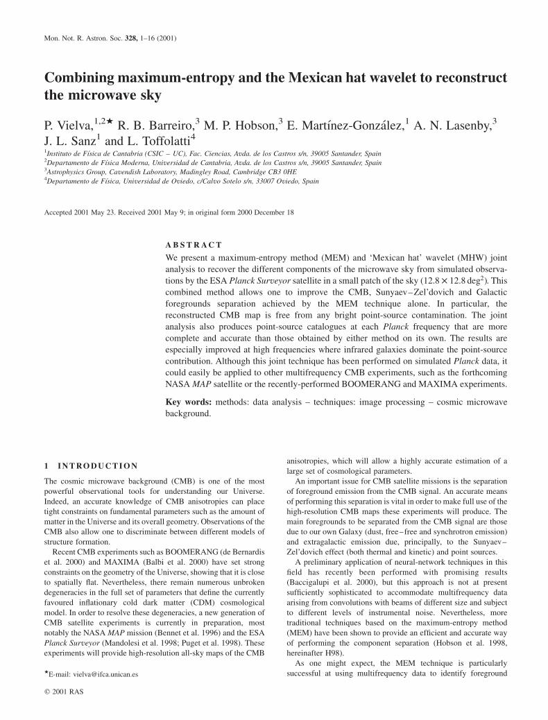
Combining maximum-entropy and the Mexican hat wavelet to reconstructthe microwave sky

P. Vielva,1,2P R. B. Barreiro,3 M. P. Hobson,3 E. Martınez-Gonzalez,1 A. N. Lasenby,3

J. L. Sanz1 and L. Toffolatti41Instituto de Fısica de Cantabria (CSIC – UC), Fac. Ciencias, Avda. de los Castros s/n, 39005 Santander, Spain2Departamento de Fısica Moderna, Universidad de Cantabria, Avda. de los Castros s/n, 39005 Santander, Spain3Astrophysics Group, Cavendish Laboratory, Madingley Road, Cambridge CB3 0HE4Departamento de Fısica, Universidad de Oviedo, c/Calvo Sotelo s/n, 33007 Oviedo, Spain

Accepted 2001 May 23. Received 2001 May 9; in original form 2000 December 18

A B S T R A C T

We present a maximum-entropy method (MEM) and ‘Mexican hat’ wavelet (MHW) joint

analysis to recover the different components of the microwave sky from simulated observa-

tions by the ESA Planck Surveyor satellite in a small patch of the sky ð12:8 � 12:8 deg2Þ. This

combined method allows one to improve the CMB, Sunyaev–Zel’dovich and Galactic

foregrounds separation achieved by the MEM technique alone. In particular, the

reconstructed CMB map is free from any bright point-source contamination. The joint

analysis also produces point-source catalogues at each Planck frequency that are more

complete and accurate than those obtained by either method on its own. The results are

especially improved at high frequencies where infrared galaxies dominate the point-source

contribution. Although this joint technique has been performed on simulated Planck data, it

could easily be applied to other multifrequency CMB experiments, such as the forthcoming

NASA MAP satellite or the recently-performed BOOMERANG and MAXIMA experiments.

Key words: methods: data analysis – techniques: image processing – cosmic microwave

background.

1 I N T R O D U C T I O N

The cosmic microwave background (CMB) is one of the most

powerful observational tools for understanding our Universe.

Indeed, an accurate knowledge of CMB anisotropies can place

tight constraints on fundamental parameters such as the amount of

matter in the Universe and its overall geometry. Observations of the

CMB also allow one to discriminate between different models of

structure formation.

Recent CMB experiments such as BOOMERANG (de Bernardis

et al. 2000) and MAXIMA (Balbi et al. 2000) have set strong

constraints on the geometry of the Universe, showing that it is close

to spatially flat. Nevertheless, there remain numerous unbroken

degeneracies in the full set of parameters that define the currently

favoured inflationary cold dark matter (CDM) cosmological

model. In order to resolve these degeneracies, a new generation of

CMB satellite experiments is currently in preparation, most

notably the NASA MAP mission (Bennet et al. 1996) and the ESA

Planck Surveyor (Mandolesi et al. 1998; Puget et al. 1998). These

experiments will provide high-resolution all-sky maps of the CMB

anisotropies, which will allow a highly accurate estimation of a

large set of cosmological parameters.

An important issue for CMB satellite missions is the separation

of foreground emission from the CMB signal. An accurate means

of performing this separation is vital in order to make full use of the

high-resolution CMB maps these experiments will produce. The

main foregrounds to be separated from the CMB signal are those

due to our own Galaxy (dust, free–free and synchrotron emission)

and extragalactic emission due, principally, to the Sunyaev–

Zel’dovich effect (both thermal and kinetic) and point sources.

A preliminary application of neural-network techniques in this

field has recently been performed with promising results

(Baccigalupi et al. 2000), but this approach is not at present

sufficiently sophisticated to accommodate multifrequency data

arising from convolutions with beams of different size and subject

to different levels of instrumental noise. Nevertheless, more

traditional techniques based on the maximum-entropy method

(MEM) have been shown to provide an efficient and accurate way

of performing the component separation (Hobson et al. 1998,

hereinafter H98).

As one might expect, the MEM technique is particularly

successful at using multifrequency data to identify foregroundPE-mail: vielva@ifca.unican.es

Mon. Not. R. Astron. Soc. 328, 1–16 (2001)

q 2001 RAS

emission from physical components whose spectral signatures are

(reasonably) well known. It is therefore not surprising that the most

problematic foreground to remove is that due to extragalactic point

sources. These differ from the other components in the important

respect that the spectral behaviour of point sources differs from one

source to the next and, moreover, is notoriously difficult to predict.

We can, however, make some headway by at least identifying the

likely populations of point sources at different observing frequen-

cies. Our knowledge of point-source populations is increasing with

new observations, but there are still great uncertainties. In the

absence of extensive observations at microwave frequencies, the

currently-favoured approach is to use the Toffolatti et al. (1998)

model, which provides an estimate of point-source populations

based on existing observations and basic physical mechanisms.

This model can be used to generate simulated point-source

emission at different observing frequencies. From 30 to 100 GHz,

the main point-source emission is due to radio selected flat-

spectrum AGNs (radio-loud quasars, blazars, etc.). From 300 to

900 GHz, infrared selected sources – starburst and late-type

galaxies at intermediate-to-low redshift and high-redshift ellip-

ticals – account for most point-source emission. At intermediate

frequencies, both populations contribute approximately equally.

The problem of removing emission due to point sources from

CMB observations has been addressed by several authors. For

example, Tegmark & Oliveira-Costa (1998, hereinafter TOC98)

suggest a straightforward harmonic filter technique that is

optimized to detect and subtract point sources, whereas Hobson

et al. (1999, hereinafter H99) propose treating point-source

emission as an additional generalized ‘noise’ contribution within

the framework of the MEM approach discussed in H98. Tenorio

et al. (1999) present a wavelet technique to subtract point sources,

but the wavelet basis used in this work is not the optimal one for

this purpose. This point is addressed in Sanz, Herranz & Martınez-

Gonzalez (2000), where it is shown that the ‘Mexican hat’ wavelet

(MHW) is in fact optimal for detecting point sources under

reasonable conditions, the most important assumption being that

the beam is well approximated by a Gaussian.

The application of this wavelet to realistic simulations has been

presented in Cayon et al. (2000, hereinafter C00) and extended in

Vielva et al. (2001, hereinafter V01). The main advantage of the

MHW method over the previous work is that the algorithm does not

require any assumptions to be made regarding the statistical

properties of the point-source population or the underlying

emission from the CMB (or other foreground components).

The aim of this paper is to show how the MEM and MHW

approaches are in fact complementary and can be combined to

improve the accuracy of the separation of diffuse foregrounds from

the CMB and increase the number of points sources that are

identified and successfully subtracted. The technique proposed in

this paper is as follows. First, we apply the MHW to the

multifrequency simulated Planck maps to detect the brightest point

sources at each observing frequency, which are subtracted from the

original data. The MEM algorithm is then applied to these

processed maps in order to recover the rest of the components of

the microwave sky. These reconstructed components are then used

as inputs to produce ‘mock’ data and subtracted from the original

data maps. Since we expect our reconstructions to be reasonably

accurate, the residuals maps obtained in this way would mostly

contain noise and the contribution from point sources. Finally, we

apply the MHW on these residuals maps in order to recover a more

complete and accurate point-source catalogue.

In this paper the combined method is applied to simulated

observation by the Planck satellite, but the technique could easily

be applied to MAP data or to existing multifrequency observations

by the BOOMERANG or MAXIMA balloon experiments. The

paper is organized as follows. In the next section we present a brief

overview of the MEM and MHW techniques, outlining in

particular the advantages and shortcomings of each approach. We

then explain why the two approaches can be successfully combined

to produce a more powerful joint analysis scheme. In Section 3 we

summarize how the simulated Planck observations were

performed. In Section 4 we present the results of a component

separation based on the new joint analysis method, and discuss the

improved accuracy of the reconstructions of the diffuse

components. In Section 5 we concentrate on the recovery of the

point sources themselves and discuss the construction of point-

source catalogues from Planck observations. Finally, our

conclusions are presented in Section 6.

2 T H E M E M A N D M H W T E C H N I Q U E S

In this section, we briefly review the MEM and MHW techniques.

A complete description of the MEM component separation

algorithm can be found in H98. In addition, H99 describes how to

include point sources into the MEM formalism. We therefore

provide only a basic outline of the approach. The MHW method is

introduced in C00 and extended in V01, and so again we give only

a basic summary.

2.1 The maximum-entropy method

If we observe the microwave sky in a given direction x at nf

different frequencies, we obtain an nf-component data vector that

contains, for each frequency, the temperature fluctuations

convolved with the beam in this direction plus instrumental

noise. The nth component of the data vector in the direction x may

be written as

dnðxÞ ¼

ðBnðjx 2 x0jÞ

Xnc

p¼1

Fnpspðx0Þ d2x0 1 jnðxÞ1 enðxÞ: ð1Þ

In this expression we distinguish between the contributions from

the point sources and the nc physical components for which it is

assumed the spectral behaviour is constant and reasonably well-

defined (over the observed patch of sky). The latter are collected

together in a signal vector with nc components, such that sp(x) is

the signal from the pth physical component at some reference

frequency n0. The corresponding total emission at the observing

frequency n is then obtained by multiplying the signal vector by the

nf � nc frequency response matrix Fnp, which includes the spectral

behaviour of the considered components as well as the

transmission of the n th frequency channel. This contribution is

then convolved with the beam profile Bn(x) of the relevant channel.

Since the individual spectral dependencies of the point sources are

very complicated, we cannot factorize their contribution in this

way and so they are added into the formalism as an extra ‘noise’

term. Thus jn is the contribution from point sources, as observed by

the instrument at the frequency n (hence, convolved with the beam

profile). Finally, en is the expected level of instrumental noise in the

n th frequency channel and is assumed to be Gaussian and isotropic.

The assumption of a spatially-invariant beam profile in Equation

(1) allows us to perform the reconstruction more effectively by

working in Fourier space, since we may consider each k-mode

independently (see H98). Thus, in matrix notation, at each mode

2 P. Vielva et al.

q 2001 RAS, MNRAS 328, 1–16

we have

d ¼ Rs 1 j 1 e ¼ Rs 1 z; ð2Þ

where d, j and e are column vectors each containing nf complex

components and s is a column vector containing nc complex

components. In the second equality we have combined the

instrumental noise vector e and the point-source contribution j into

a single ‘noise’ vector z. The response matrix R has dimensions

nf � nc and its elements are given by RnpðkÞ ¼ ~BnðkÞFnp. The aim

of any component separation/reconstruction algorithm is to invert

Equation (2) in some sense, in order to obtain an estimate s of the

signal vector at each value of k independently. Owing to the

presence of noise, and the fact that the response matrix R is not

square and would, in any case, have some small eigenvalues, a

direct inversion is not possible, and so some form of regularized

inverse must be sought. Typical methods include singular-valued

decomposition, Wiener filtering or the maximum-entropy method.

The elements of the signal vector s at each Fourier mode may

well be correlated, this correlation being described by the nc � nc

signal covariance matrix C defined by

CðkÞ ¼ ksðkÞs †ðkÞl; ð3Þ

where the dagger denotes the Hermitian conjugate. Moreover, if

prior information is available concerning these correlations, we

would wish to include it in our analysis. We therefore introduce the

vector of ‘hidden’ variables h, related to the signal vector by

s ¼ Lh; ð4Þ

where the nc � nc lower triangular matrix L is obtained by

performing a Cholesky decomposition of the signal covariance

matrix C ¼ LLT. The reconstruction is then performed entirely in

terms of h and the corresponding reconstructed signal vector is

subsequently found using Equation (4).

Using Bayes’s theorem, we choose our estimator h of the hidden

vector to be that which maximizes the posterior probability given

by

PrðhjdÞ/PrðdjhÞ PrðhÞ; ð5Þ

where Pr (djh) is the likelihood of obtaining the data given a

particular hidden vector and Pr (h) is the prior probability that

codifies our expectations about the hidden vector before acquiring

any data.

As explained in H99, the form of the likelihood function in

Equation (5) is given by

PrðdjhÞ/ expð2z†N21zÞ/exp½2ðd 2 RLhÞ†N21ðd 2 RLhÞ�;

ð6Þ

where in the last line we have used Equation (2). The noise

covariance matrix N has dimensions nf � nf and at any given

k-mode is given by

NðkÞ ¼ kzðkÞz†ðkÞl: ð7Þ

Therefore, at a given Fourier mode, the n th diagonal element of Ncontains the ensembled-averaged power spectrum at that mode of

the instrumental noise plus the point-source contribution to the n th

frequency channel. The off-diagonal terms give the cross-

correlations between different channels; if the noise is uncorrelated

between channels, only the point sources contribute to the off-

diagonal elements.

For the prior Pr (h) in Equation (5), we assume the entropic

form

PrðhÞ/exp½aSðh;mÞ�; ð8Þ

where S(h,m) is the cross entropy of the complex vectors h and m,

where m is a model vector to which h defaults in the absence of

data. The form of the cross entropy for complex images and the

Bayesian method for fixing the regularizing parameter a are

discussed in H98. We note that, in the absence of non-Gaussian

signals, the entropic prior Equation (8) tends to the Gaussian prior

implicitly assumed by Wiener filter separation algorithms, and so

in this case the two methods coincide.

The argument of the exponential in the likelihood function of

Equation (6) may be identified as (minus) the standard x 2 misfit

statistic, so we may write Pr ðdjhÞ/exp½2x 2ðhÞ�. Substituting this

expression, together with that for the prior probability given in

Equation (8), into Bayes’s theorem, we find that maximizing the

posterior probability Pr (hjd) with respect to h is equivalent to

minimizing the function

FðhÞ ¼ x 2ðhÞ2 aSðh;mÞ:

This minimization can be performed using a variable metric

minimizer (Press et al. 1994) and requires only a few minutes of

CPU time on a Sparc Ultra workstation.

2.2 The Mexican hat wavelet method

The MHW technique presented by C00 and V01 for identifying

and subtracting point sources operates on individual data maps.

Let us consider the two-dimensional data map dn(x) at the

frequency n. If the map contains point sources at positions bi

with fluxes or amplitudes Ai, together with contributions from other

physical components and instrumental noise, then the data map is

given by

dnðxÞ ¼ jnðxÞ1 nnðxÞ ¼i

XAiBnðx 2 biÞ1 nnðxÞ; ð9Þ

where Bn(x) is the beam at the observing frequency n, and in this

case the generalized ‘noise’ nn(x) is defined as all contributions to

the data map aside from the point sources.

For the ith point source, we may define a ‘detection level’

D ¼Ai/V

sn

; ð10Þ

where V is the area under the beam and sn is the dispersion of the

generalized noise field nn(x). In general, the detection level D will

be much less than unity for all but the few brightest sources. This is

the usual problem one faces when attempting to identify point

sources directly in the data map.

As explained in C00, instead of attempting the identification in

real space, one can achieve better results by first transforming to

wavelet space. For a two-dimensional data map dn(x), we define

the continuous isotropic wavelet transform by

wdðR; bÞ ¼

ðd2x

1

R 2cjx 2 bj

R

� �dnðxÞ; ð11Þ

where w(R,b) is the wavelet coefficient associated with the scale R

at the point b (where the wavelet is centred). The function c(jxj) is

the mother wavelet, which is assumed to be isotropic and satisfies

CMB observations: combined MEM/MHW analysis 3

q 2001 RAS, MNRAS 328, 1–16

the conditions

ðd2xcðxÞ ¼ 0 ðcompensationÞðd2xjcðxÞj

2¼ 1 ðnormalizationÞ

Cc ¼ ð2pÞ2Ð1

0dk k 21j ~cðkÞj

2, 1 ðadmissibilityÞ;

where c denotes the Fourier transform of c, x ¼ jxj and k ¼ jkj.

The wavelet coefficients given by Equation (11) characterize the

contribution from structure on a scale R to the value of the map at

the position b.

By analogy with Equation (10), in wavelet space, we define

the detection level for the ith point source (as a function of scale R)

by

DwðRÞ ¼wjðR; biÞ

swnðRÞ

; ð12Þ

where wj(R,bi) is the wavelet coefficient of the field jn(x) at the

location of the ith point source, and s2wnðRÞ is the dispersion of the

wavelet coefficients wn(R, b) of the generalized noise field nn(x). It

is straightforward to show that

s2wnðRÞ ¼ 2p

ðkmax

kmin

dk kPðkÞj ~cðRkÞj2; ð13Þ

where P(k) is the power spectrum of nn(x). The integral limits, kmin

and kmax, correspond to the maximum and minimum scales of the

sky patch analysed, i.e. the patch and pixel scales, respectively.

The detection level Dw(R) in wavelet space will have a

maximum value at some scale R ¼ R0. This scale is practically the

same for all point sources, and may be found by solving

dDwðR0Þ=dR ¼ 0. In general, the optimal scale is of the order of the

beam dispersion sa (see V01, section 3, for a discussion about how

the noise and the coherence scale of the background determine the

optimal scale). In order that the wavelet coefficients are optimally

sensitive to the presence of the point source, we must make the

value of Dw(R0) as large as possible. This is achieved through an

appropriate choice both of the mother wavelet c(x) and the optimal

scale. If the beam profile is Gaussian and the power spectrum of the

generalized noise field is scale-free, Sanz et al. (2000) show that,

for a wide range of spectral indices of the power spectrum, the

Mexican hat wavelet is optimal. The two-dimensional MHW is

given by

cðxÞ ¼1ffiffiffiffiffiffi2pp 2 2

x

R

� �2� �

e 2x 2 /2R 2

; ð14Þ

from which we find

wjðR; biÞ ¼ 2ffiffiffiffiffiffi2pp Ai

V

ðR/saÞ2

ð1 1 ðR/saÞ2Þ2

; ð15Þ

where Ai is the amplitude of the ith point source, V is the area

under the Gaussian beam and sa is the beam dispersion. In

Equation (15) it is assumed that any overlap of the (convolved)

point sources is negligible. That is a good approximation for the

brightest point sources, the ones that the MHW is able to detect. In

fact, the number of point sources detected at each frequency (see

Table 1) corresponds only to a small percentage of the number of

resolution elements (see Table 2) contained at each Planck

frequency channel (,6 per cent at 30 GHz, the most unfavourable

case). Therefore, the probability of finding two or more bright

point sources inside the same resolution element is very low. The

advantage of identifying point sources in wavelet space rather than

Table 1. The point-source catalogues obtained using the MHW alone (MHWc), MEM alone (MEMc) and the joint analysis method(M&Mc). For each Planck observing frequency, we list the number of sources detected, the flux limit of the catalogue and the average ofthe absolute value of the percentage error for the amplitude estimation. The numbers in brackets in the second column indicate thenumber of point sources that are detected by the 5swd

criterion (see text for details).

MHWc MEMc M&McFrequency Number of Min Flux E Number of Min Flux E Number of Min Flux E(GHz) detections (Jy) (per cent) detections (Jy) (per cent) detections (Jy) (per cent)

30 15 (4) 0.13 14.0 32 0.09 14.9 30 0.09 14.044 11 (3) 0.27 11.2 28 0.11 14.2 28 0.11 13.270 7 (5) 0.30 7.9 38 0.08 11.8 35 0.09 11.4

100 (LFI) 12 (3) 0.23 11.8 37 0.08 16.4 44 0.06 18.4100 (HFI) 17 (7) 0.14 14.1 72 0.04 17.3 74 0.03 17.4143 11 (4) 0.16 18.0 0 – – 5 0.32 12.4217 15 (5) 0.08 14.4 0 – – 5 0.25 15.4353 16 (10) 0.15 14.3 38 0.08 28.7 37 0.08 34.9545 37 (29) 0.29 14.1 89 0.18 26.4 121 0.15 17.2857 306 (86) 0.30 16.5 458 0.23 20.6 492 0.19 19.5

Table 2. Basic observational parameters of the 10frequency channels of the Planck Surveyor satellite. Columntwo lists the fractional banwidths. The FWHM in columnthree assumes a Gaussian beam. In column four theinstrumental noise level is DT (mK) per resolution elementfor 12 months of observation.

Frequency Fractional bandwidth FWHM snoise

(GHz) (Dnn ) (arcmin) (mK)

30 0.20 33.0 4.444 0.20 23.0 6.570 0.20 14.0 9.8100 (LFI) 0.20 10.0 11.7100 (HFI) 0.25 10.7 4.6143 0.25 8.0 5.5217 0.25 5.5 11.7353 0.25 5.0 39.3545 0.25 5.0 400.7857 0.25 5.0 18182

4 P. Vielva et al.

q 2001 RAS, MNRAS 328, 1–16

real space may then be characterized by the amplification factor

A ¼ DwðR0Þ

D¼ 2

ffiffiffiffiffiffi2pp ðR0/saÞ

2

ð1 1 ðR0/saÞ2Þ2

sn

swnðR0Þ

: ð16Þ

In practice, it is clear that we do not have access to the wavelet

coefficients of the fields jn(x) and nn(x) separately, but only to the

wavelet coefficients of the total data map dnðxÞ ¼ jnðxÞ1 nnðxÞ.

Nevertheless, if the detection level Dw(R) for the ith point source is

reasonably large, we would expect wjðR; biÞ < wdðR; biÞ. Also, if

we assume that the power spectrum of the point-source emission is

negligible as compared with that of the generalized noise field, then

swnðRÞ < swd

ðRÞ. Thus our algorithm for detecting point sources is

as follows. Using the above approximations, we first calculate the

optimal scale R0. We then calculate the wavelet transform wd(R0, b)

of the data map at the optimal scale. The wavelet coefficients are

then analysed to find sets of connected pixels above a certain

threshold swd(R0). The maxima of these spots are taken to

correspond to the locations of the point sources.

For every point source detected in the above way, we then go on

to estimate its flux. This is achieved by performing a multiscale fit

as follows. For each point-source location bi, the wavelet transform

wd(R, bi) is calculated at a number of scales R and compared with

the theoretical curve Equation (15). This comparison is performed

by calculating the standard misfit statistic

x 2 ¼ ½w ðexpÞ 2 w ðtheoÞ�TV21½w ðexpÞ 2 w ðtheoÞ�; ð17Þ

where the kth element of the vector w (exp) is wðexpÞd ðRk; biÞ (and

similarly for the vector of theoretical wavelet coefficients). The

matrix V is the empirical covariance matrix of the wavelet

coefficients on different scales, which is given by

Vjk ¼ kwðexpÞd ðRj; bÞw

ðexpÞd ðRk; bÞl; ð18Þ

where the average is over position b.

2.3 MEM and MHW joint analysis

In H99, the MEM technique is shown to be effective at performing

a full component separation in the presence of point sources. In

particular, the reconstructed maps of the separate diffuse

components contain far less point-source contamination than the

input data maps. Moreover, by comparing the true data maps with

simulated data maps produced from the separated components, it is

possible to obtain point-source catalogues at each observing

frequency. Nevertheless, the MEM approach does have its

limitations. Since the point sources are modelled as an additional

generalized noise component, it is not surprising that MEM

performs well in identifying and removing the large number of

point sources with low-to-intermediate fluxes. However, it is rather

poorer at removing the contributions from the brightest point

sources. These tend to remain in the reconstructed maps of the

separate diffuse components, although with much reduced

amplitudes.

The MHW technique, on the other hand, performs best when

identifying and removing the brightest point sources. Indeed, in

detecting bright sources the MHW technique generally out-

performs other techniques such as SEXTRACTOR (Bertin & Arnouts

1996) and standard harmonic filtering (TOC98). Moreover, the

amplitudes of the bright sources are also accurately estimated. For

weaker sources, however, the MHW technique performs more

poorly by either inaccurately estimating the flux or failing to detect

the source altogether.

The strengths and weaknesses of the MEM and MHW

approaches clearly indicate that they are complementary

techniques, and that a combined approach might lead to improved

results as compared with using each method independently. We

thus propose the following method for analysing multifrequency

observations of the CMB that contain point-source contamination.

First, the data map at each observing frequency is analysed

separately using the MHW in order to detect and remove as many

bright point sources as possible and obtain accurate estimates of

their fluxes. The processed data maps are then taken as the inputs to

the generalized MEM approach discussed in H99. As we will

demonstrate in Section 4, the MEM analysis of these processed

maps leads to more accurate reconstructed maps of the separate

diffuse components. This leads in turn to more accurate residual

maps between the true input data with the data simulated from the

reconstructions. These residual maps are then analysed with the

MHW in order both to refine the original estimates of the fluxes of

the bright point sources and to detect fainter sources. Thus, the

joint analysis not only gives a more complete point-source

catalogue, but also improves the quality of the reconstructed maps

of the CMB and other foreground components.

3 S I M U L AT E D O B S E RVAT I O N S

As mentioned in the introduction, the joint analysis technique can

be applied to any multifrequency observations of the CMB that

may contain point-source emission. Thus, for example, the method

could straightforwardly be applied to the existing BOOMERANG

or MAXIMA data sets, or to observations by the forthcoming

NASA MAP satellite. Nevertheless, in order to test the capabilities

of the joint analysis method to the fullest extent, in this paper we

apply it to simulated observations by the proposed ESA Planck

Surveyor satellite. The basic observational parameters of the

Planck mission instruments (HFI and LFI) are listed in Table 2.

The simulated data are similar to those used in H99. They

include contributions from the primordial CMB, the thermal and

kinetic Sunyaev–Zel’dovich effects, extragalactic point sources,

Galactic thermal dust and free–free and synchrotron emission.

Figure 1. The 12:8 � 12:8 deg2 realizations of the six input components

used to produce the simulated Planck data. They include contributions from

the CMB, the thermal and kinematic Sunyaev–Zel’dovich (SZ) effects,

extragalactic point sources, and Galactic thermal dust, free–free and

synchrotron emission. Each component is plotted at 300 GHz and has been

convolved with a Gaussian beam of FWHM 5 arcmin (the highest

resolution expected for the Planck satellite). The map units are equivalent

thermodynamic temperature in mK.

CMB observations: combined MEM/MHW analysis 5

q 2001 RAS, MNRAS 328, 1–16

Aside from the point sources, we assume that the emission of each

physical component can be factorized into a spatial template at

300 GHz with a known frequency dependence. In Fig. 1 we have

plotted the six component templates at 300 GHz. Each map covers

a 12:8 � 12:8-deg2 patch of sky and has been convolved with a

Gaussian beam with FWHM 5 arcmin (i.e. the highest Planck

resolution).

The CMB map is a Gaussian realization of a spatially-flat

inflationary/CDM model with Vm ¼ 0:3 and VL ¼ 0:7, for which

the C‘ coefficients were generated using CMBFAST (Seljak &

Zaldarriaga 1996). The thermal Sunyaev–Zel’dovich map is taken

from the simulations of Diego et al. (2001) and assume the same

cosmological model as that used for the CMB. The kinetic SZ field

is produced by assuming that the line-of-sight cluster velocities are

drawn from a Gaussian distribution with zero mean and rms

400 km s21. The extragalactic point-source simulations adopt the

model of Toffolatti et al. (1998) and also assume the same

cosmological model.

The Galactic thermal dust emission is created using the template

of Finkbeiner, Davis & Schlegel (1999). The frequency

dependence of the dust emission is assumed to follow a grey-

body function characterized by a dust temperature of 18 K and an

emissivity b ¼ 2. The distribution of Galactic free–free emission

is poorly known. Current experiments such as the H-a Sky Survey1

and the WHAM project2 should soon provide maps of Ha emission

that could be used as templates. For the time being, however, we

create a free–free template that is correlated with the dust emission

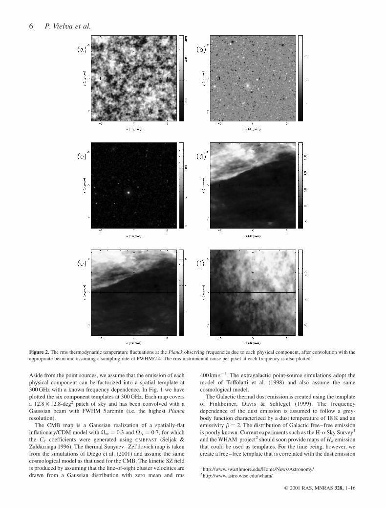
Figure 2. The rms thermodynamic temperature fluctuations at the Planck observing frequencies due to each physical component, after convolution with the

appropriate beam and assuming a sampling rate of FWHM/2.4. The rms instrumental noise per pixel at each frequency is also plotted.

1 http://www.swarthmore.edu/Home/News/Astronomy/2 http://www.astro.wisc.edu/wham/

6 P. Vielva et al.

q 2001 RAS, MNRAS 328, 1–16

Figure 3. The 12:8 � 12:8 deg2 data maps observed at each of the ten Planck frequency channels listed in Table 2. The panels correspond to the frequencies: (a)

30 GHz, (b) 44 GHz, (c) 70 GHz, (d) 100 GHz-lfi, (e) 100 GHz-hfi, (f) 143 GHz, (g) 217 GHz, (h) 353 GHz, (i) 545 GHz and (j) 857 GHz. The units are

equivalent thermodynamic temperature in mK.

CMB observations: combined MEM/MHW analysis 7

q 2001 RAS, MNRAS 328, 1–16

in the manner proposed by Bouchet, Gispert & Puget (1996). The

frequency dependence of the free–free emission is assumed to vary

as In/n20:16, and is normalized to give an rms temperature

fluctuation of 6.2mK at 53 GHz. Finally, the synchrotron spatial

template has been produced using the all-sky map of Fosalba &

Giardino3. This map is an extrapolation of the 408-MHz radio map

of Haslam et al. (1982), from the original 1-deg resolution to a

resolution of about 5 arcmin. The additional small-scale structure is

assumed to have a power-law power spectrum with an exponent of

23. We have continued this extrapolation to 1.5 arcmin following

the same power law. The frequency dependence is assumed to be

In/n20:9 and is normalized to the Haslam 408-MHz map.

To simulate the observed data in a given Planck frequency

channel, each of the physical components discussed above is first

projected to the relevant frequency and the contributions are

summed. The predicted point-source emission for the frequency is

then added, and the resulting total sky emission is convolved with a

Gaussian beam of the appropriate FWHM. Finally, independent

pixel noise is added, with corresponding rms from Table 2. In Fig. 2

we give the rms thermodynamic temperature fluctuations in the

data at each Planck observing frequency due to each physical

component and the instrumental noise. In Fig. 3 we plot the

simulated Planck observations in each frequency channel, all the3 ftp://astro.estec.esa.nl/pub/synchrotron

Figure 4. The reconstructed maps for each of the physical components: (a) CMB, (b) kinetic SZ effect, (c) thermal SZ effect, (d) Galactic dust, (e) Galactic

free–free and (f) Galactic synchrotron emission. Point sources have been subtracted from the data maps using the Mexican hat algorithm before applying

MEM. Each component is plotted at 300 GHz and has been convolved with a Gaussian beam of FWHM 5 arcmin. The map units are equivalent thermodynamic

temperature in mK.

8 P. Vielva et al.

q 2001 RAS, MNRAS 328, 1–16

components are included: CMB, dust, free–free, synchrotron,

kinetic and thermal SZ effects and point-source emission as well as

instrumental noise.

4 F O R E G R O U N D S E PA R AT I O N

We have applied the method outlined in Section 2.3 to the

simulated Planck data described above. We have assumed

knowledge of the azimuthally averaged power spectra of the six

input components in Fig. 1, together with the azimuthally averaged

cross power spectra between them (see H98 for more details).

Using the model of Toffolatti et al. (1998), we have also introduced

the power spectrum of the point sources at each frequency channel,

including cross power spectra between channels, and account for

this contaminant as an extra noise term (see H99 for more details).

However, the recovery of the main components and point sources

does not depend critically on this assumption, as will be discussed

later.

The resulting reconstructions of the physical components at a

reference frequency of 300 GHz are shown in Fig. 4. The maps

have been plotted using the same grey-scale as in Fig. 1 to allow a

straightforward comparison. In Fig. 5, we plot the residuals for

each component, obtained by subtracting the input maps from the

reconstructions.

We can see that the main input components have been faithfully

recovered with no obvious visible contamination from point

sources. This is because the MHW subtraction algorithm is

efficient at removing the brightest point sources, whereas MEM

Figure 5. The reconstruction residuals obtained from subtracting the input maps of Fig. 1 from the reconstructed maps of Fig. 4. The panels correspond to: (a)

CMB, (b) kinetic SZ effect, (c) thermal SZ effect, (d) Galactic dust, (e) Galactic free–free, (f) Galactic syncrotron emission.

CMB observations: combined MEM/MHW analysis 9

q 2001 RAS, MNRAS 328, 1–16

has greatly reduced the contamination due to fainter sources. We

give the rms reconstruction errors for each component in Table 3.

In particular, we note that the CMB has been recovered very

accurately, although the residuals map does show some weak

contamination due to low-amplitude point sources. Indeed, the rms

reconstruction error for this component is ,7.7mK, which

corresponds to an accuracy of ,6.8 per cent as compared with

the rms of the input CMB map (see Table 3). Even more impressive

is the reconstruction of the dust map. None of the numerous point

sources present in the highest frequency channel maps are visible

in the reconstruction. This is also confirmed by inspecting the

residual map. The main features of the free–free emission are also

recovered, mostly owing to its high correlation with the dust.

Again, the reconstruction shows no evidence of point-source

contamination. For the synchrotron component, the recovered

emission is basically a lower resolution image of the input map.

This is expected since only the lowest frequency channels provide

useful information about this component, and these channels also

have the lowest angular resolutions. Although the reconstructed

synchrotron map is mostly free of point sources, some residual

contamination remains. This contamination corresponds to a few

medium-amplitude point sources that are present in the lowest

frequency channels, although they are not clearly visible in the

data. These sources are too weak to be detected using the MHW

algorithm but at the same time they are not well characterized by

the generalized noise approach assumed in MEM.

As pointed out in H99, one must be careful when comparing the

amplitude of the residual point sources still contaminating the

reconstructions with the corresponding amplitudes of the point

sources in the data maps. The reconstructions are calculated at a

reference frequency of 300 GHz and those sources remaining in the

residuals maps are projected in frequency according to the spectral

dependence of the component they contaminate. In addition, we

have to take into account the different resolution of the Planck

frequency channels. For example, the contaminating point source

in the middle right-hand side of the synchrotron residuals map has

an amplitude of . 0.15mK after convolution with a Gaussian beam

of FWHM 33 arcmin (the resolution of the 30-GHz Planck

frequency channel). Following the spectral dependence of the

synchrotron component, this projects to 17.5mK at 30 GHz. This

value should be compared with the amplitude of the point source at

the same frequency, which is around 150mK. Therefore, MEM has

succeeded in reducing the contamination due to this point source

by almost a factor of ten.

The recovery of the thermal SZ effect is quite good. Most of the

bright clusters have been reproduced whereas only a few point

sources have been misidentified as clusters. At the reference

frequency of 300 GHz, these misidentified point sources appear

mostly as negative features. Finally, as expected, the reconstruction

of the kinetic SZ is quite poor and one detects only a few clusters

whose corresponding thermal SZ effect is large.

We have also calculated the power spectrum of the reconstructed

component maps and found that the accuracy is very similar to that

found in H99, so we do not plot them again here. The effect of first

applying the MHW to the data maps before the MEM analysis is

not so obvious when considering the power spectra of the

reconstructions, since only a small percentage of pixels are affected

by residual point sources and this has little effect in the recovered

spectrum. Nevertheless, the removal of the point-source contami-

nation is vital if one wishes to probe the Gaussian character of the

CMB, as well as to study properties of the other foreground

components.

To understand better the effect of performing the MHW analysis

on the data maps prior to the MEM algorithm, we have also carried

out a component separation for the case where the MHW step is not

performed; this corresponds to the method in H99. In Fig. 6, we

show the difference between the reconstructions obtained using the

combined MHW/MEM technique and those obtained using MEM

alone. Thus these maps display the point sources that have been

successfully removed by the MHW, which would otherwise be

present in the reconstructions. By comparing with the data, we can

also see how the point sources present in the different frequency

channels would affect a given component if not carefully

subtracted. Particularly impressive is the removal from the dust

and free–free reconstructions of the large number of point sources

that were present in high-frequency data channels. For the CMB,

the MHW has subtracted a few very bright point sources, which

dominated the contribution of this contaminant in the intermediate

frequency channels. We also note that the MHW has removed a few

from the synchrotron reconstruction that were present in the

lowest channels. The reconstructions of the thermal and kinetic

SZ effects have also been improved since a lower number of

point sources have been misidentified as clusters; these sources

were detected by the MHW mainly in the highest channels of the

LFI. The rms reconstructions errors when MEM is used without

a previous subtraction of point sources by the MHW are also

given in Table 3.

Finally, we can also study how our reconstructions are affected if

we do not assume full power spectrum information. Thus, we have

repeated our joint analysis of the simulated Planck observations for

the case where we assume that ‘2C‘ is constant for each

component out to the highest measured Fourier mode. The level of

the flat power spectrum for each component is, however, chosen so

that the total power in each component is approximately that

observed in the input maps in Fig. 1. Furthermore, no information

about the cross power spectra between different components is

given. Regarding the point sources, the true azimuthally averaged

power spectrum is again assumed to account for their contribution

as an extra noise term but cross-correlations between different

frequency channels are ignored. The quality of the reconstructions

of the main components is actually very similar to the case when

full power spectrum information is given. In particular, the

accuracy of the CMB reconstructed map is only slightly worse with

an rms error of 8.2mK as compared with 7.7mK in the former case.

Moreover, the reconstruction is again free from obvious

contamination due to point sources. Similarly, the dust component

has been faithfully recovered with a rms error of 3.0mK versus

Table 3. The rms in mK of the reconstruction residualssmoothed with a 5-arcmin FWHM Gaussian beam with andwithout the initial subtraction of bright point sources usingthe MHW. Full power spectrum information has beenassumed. For comparison, the rms of the input maps shownin Fig. 1 are also given. Results are given for the referencefrequency 300 GHz.

Component Input Error Errorrms (with MHW) (without MHW)

CMB 112.3 7.68 8.62Kinetic SZ 0.69 0.70 0.70Thermal SZ 5.37 4.64 4.66Dust 55.8 2.68 3.39Free–free 0.66 0.22 0.24Synchrotron 0.32 0.11 0.12

10 P. Vielva et al.

q 2001 RAS, MNRAS 328, 1–16

2.7mK when full power spectrum is assumed. The main features of

the synchrotron and thermal SZ effect are also recovered, although

the reconstructions are poorer. In particular, the contamination due

to point sources is slightly increased in the thermal SZ

reconstructed map. Finally, the weakest components, free–free

emission and kinetic SZ effect, are lost in this case and the

reconstructions have simply defaulted to zero in the absence of any

useful information.

5 R E C OV E RY O F P O I N T S O U R C E S

The previous section focused on the recovery of the six physical

component maps shown in Fig. 1. However, a major aim of the

Planck mission is also to compile point-source catalogues at each

of its observing frequencies. In this section, we compare the

catalogues obtained using MEM alone (i.e., without a previous

subtraction of bright sources detected by the MHW), MHW alone

and the joint analysis method M&M.

The MHW catalogue (MHWc) is produced in the manner

explained in V01, through the so called 50 per cent error criterion

(see the previous work for more details in detection criteria). In

short, each of the data maps of Fig. 3 is independently analysed

with the MHW. Those coefficients above 2swdat the optimal

wavelet scale are identified as point-source candidates. A

Figure 6. The residuals obtained by subtracting the reconstructed maps shown in Fig. 4 from the reconstructions achieved when the MHW is not used to

perform an initial point-source removal. Both reconstructions were smoothed with a Gaussian beam of FWHM 5 arcmin and correspond to a frequency of

300 GHz. The different panels are: (a) CMB, (b) kinetic SZ effect, (c) thermal SZ effect, (d) Galactic dust, (e) Galactic free–free and (f) Galactic synchrotron

emission. The map units are equivalent thermodynamic temperature in mK.

CMB observations: combined MEM/MHW analysis 11

q 2001 RAS, MNRAS 328, 1–16

multiscale fit is then performed in order to estimate their amplitude

and those wavelet coefficients with a non-acceptable fit are

discarded. We then look for the flux above which at least 95 per

cent of the detected point sources have a relative error #50 per

cent. This gives our estimation of the flux limit. Thus, the number

of detections at a given channel is given by those point sources with

an estimated amplitude above the flux limit. In practice, we also

use multifrequency information to include those point sources that,

having an error larger than 50 per cent or an insufficiently good fit,

have been detected in an adjacent channel (although in most

channels this only accounts for a very small fraction of the detected

point sources). The error is defined as: E ¼ jA 2 A ej/A, where A is

the flux of the simulated source and A e that of the estimated one.

Although the MHW catalogue (hereafter MHWc) is obtained in

the same way as that of V01, the results here differ slightly. This

apparent discrepancy is due to the different sampling rates that

have been considered in each case. V01 assumes pixel sizes of 1.5,

3 and 6 arcmin for the different Planck channels, whereas in this

work the pixel size is given by a fixed sampling of 2.4, following by

a regridding to pixels of size 1.5 arcmin. Therefore, the number of

detected point sources and fluxes of V01 and this paper are not

directly comparable.

Nevertheless, not all the point sources in the MHWc are

subtracted from the original maps prior to performing the MEM

analysis. In theory, giving as much information as available should

improve the MEM results. However, when using the 50 per cent

error criterion a significant number of point sources, especially at

the 545 and 857 GHz channels, are estimated with a large error.

Therefore, if this information is given to MEM (by subtracting

these sources from the original maps), we are misleading the MEM

algorithm. To avoid this unwanted effect, the point sources

subtracted from the maps should be those with the lowest errors in

the amplitude estimation. We need a more robust criterion than that

of the 50 per cent error. Instead we adopt the so-called 5swd

criterion, which is also explained in V01. Briefly, we consider that

a point source has been detected if the position of its maximum is

above 5swdand its multiscale fit is acceptable.

The MEM catalogue (MEMc) and the M&M one (M&Mc) are

obtained using the method outlined in H99. First, the reconstructed

maps of Fig. 4 are used as inputs to produce ‘mock’ data. We

follow the same procedure as that used to obtain the data of Fig. 3

but, of course, we do not add instrumental noise or the point

sources. These mock data are then subtracted from the true data

(which contain the full point-source contribution). Since the

reconstructions of the six main components are reasonably

accurate and also contain very few point sources, we obtain a data

residuals map at each Planck frequency that consists mainly of the

point sources and instrumental noise. Each of these residuals

maps are then independently analysed in order to produce a

point source catalogue at each observing frequency. We point

out, however, that the residuals maps produced here differ from

those in H99. In order to concentrate on the effect of emission

from other physical components on the point-source recovery, in

H99 the instrumental noise was neglected when making the

residuals maps. Here the instrumental noise is included to obtain

a more realistic estimate of the number of point sources

recoverable from real Planck data.

Another difference with H99 is the process by which the point-

source catalogue is produced from the residuals maps. In H99, the

SEXTRACTOR package (Bertin & Arnouts, 1996) is used to detect

and estimate the amplitude of point sources. The SEXTRACTOR

package begins by fitting and subtracting an unresolved background

component, before identifying any point sources, and can lead to

ambiguities in assigning a flux detection limit. Therefore, in the

present paper, the residuals maps are instead analysed using the

MHW, since this wavelet filter is optimal for this purpose (Sanz

et al. 2000). At this point, however, it is worth pointing out some

subtleties associated with applying the MHW in these circum-

stances. In particular, for the MEMc and M&Mc, we apply the 50

per cent error criterion into the residual maps, in order to compare

with the MHWc. Clearly, this choice determines empirically the

flux limit of the catalogue (achieved by the 50 per cent error

criterion) and will depend on the assumed point-source population

model, but we expect that most models lead to similar results. In

fact, in V01 it is shown that for the Guiderdoni et al. (1998) E

model, the flux limits achieved are very similar.

In Table 1 we give, for each catalogue, the number of point

sources detected, the minimum flux achieved and the average

amplitude error in each Planck frequency channel.

In the two highest frequency channels, the joint analysis clearly

outperforms the results obtained with each of the methods

separately. This is due to the complementary nature of the two

approaches, so that bright sources are detected by MHW and

intermediate flux sources are identified by MEM. If MEM alone is

used, many of the brightest point sources remain in the MEM

reconstructions since they are not well characterized by a

generalized noise. Therefore they are either not detected in the

data residuals maps or the error in the estimated amplitude is

significantly large. However, in the joint analysis these sources are

easily detected and their fluxes accurately estimated.

Regarding the 353-GHz channel, the number of point sources

detected with M&M is comparable with the best of the individual

methods, i.e. when using MEM on its own. This is due to the fact

that the main contaminant of the residuals maps is the high level of

noise of the 353-GHz channel, which is equally present in both the

residuals obtained with MEM and with M&M. In fact, many of the

point sources have been detected (with a large error) thanks to the

multifrequency information.

The low number of point sources detected at intermediate

frequencies (217 and 143 GHz) in the M&Mc in comparison with

the MHWc can be explained as a combination of factors. First of

all, owing to the high level of noise in these channels relative to the

point-source emission, only a few point sources are detected with

the MHW in the first step of our analysis, through the 5swd

criterion. Therefore, when applying MEM, part of the emission of

the undetected point sources is left in the reconstructed

components, being mainly misidentified with CMB, which is the

dominant component at those frequencies. This has the effect of

lowering the level of the point sources in the data residuals, which

together with the high level of noise, leads to a low number of

recovered point sources.

In the low-frequency channels, the number of point sources

detected by the joint analysis is similar to that by MEM alone (the

fact that M&M does not work better than MEM alone for all the

channels may be understood as a statistical fluctuation; we expect

that with an all-sky point-source simulation, the results of the

combined method will be better than those of MEM in every

case). In this case, the MHW contribution is to improve the

amplitude estimation of a few point sources, which leads to a

lower average amplitude error. In these frequency channels,

MHW alone detects only the few brightest point sources. This is

because these channels are dominated by the CMB and the beam

FWHM is so large that the CMB and point sources have a similar

characteristic scale.

12 P. Vielva et al.

q 2001 RAS, MNRAS 328, 1–16

Regarding the estimation of point-source amplitudes, the joint

analysis also performs better than each method independently.

Although the average error in the amplitude estimation can be

larger in the M&Mc than in the MHWc owing to the detection of a

larger number of faint point sources, those point sources present in

all three catalogues are, on average, better estimated with the

combined analysis.

In Fig. 7 we plot the amplitude estimation errors for the MHWc,

MEMc and M&Mc versus the true flux (in Jy) for two

representative channels: 44 and 545 GHz. We can see that there

is a clear bias in the estimation of the amplitude of the brightest

point sources in MEMc since they remain in the reconstructions

and are therefore underestimated (corresponding to positive errors

in Fig. 7). This problem is solved when combining MEM and the

MHW. It is also obvious that a larger number of point sources and

fainter fluxes are achieved in the combined analysis with respect to

the MHW on its own.

In Fig. 8 we have plotted the sources in M&Mc, for the same

two channels, together with the input point-sources maps. We

see that the main features are very well recovered. At 44 and

545 GHz, the flux limit is comparable with the level of

instrumental noise (see the next section). Thus, to increase still

further the number of point sources detected and reach fainter

fluxes, one would need to denoise the residuals maps; this is

discussed in the next section.

We have also investigated the effect of reducing the power

spectrum information given to MEM. We find that even in the

extreme case when a flat power spectrum is assumed for the

different components, the results are not significantly different for

the M&Mc, but the quality of the MEMc is somewhat reduced,

especially in the high frequency channels. In particular, the

amplitude estimation errors are higher and the catalogue flux limit

increases slightly.

6 D I S C U S S I O N A N D C O N C L U S I O N S

The MEM (H98, H99) and the MHW (C00, V01) techniques have

complementary characteristics when recovering the microwave

Figure 7. Errors in the amplitude estimation for the MHW, MEM and joint analysis catalogues (MHWc, MEMc and M&Mc, respectively) as a function of the

flux. We plot two Planck frequencies: 44 GHz (top) and 545 GHz (bottom).

0.1 0.25 0.5 0.75 1100

80

60

40

20

0

20

40

60

80

100Error in the amplitude estimation at 44 GHz

MHWcMEMcM&Mc

0.25 0.5 1 1.5 2 2.5 3100

80

60

40

20

0

20

40

60

80

100

Flux (Jy)

Err

or(%

)

Error in the amplitude estimation at 545 GHz

MHWcMEMcM&Mc

Err

or(%

)

Flux (Jy)

CMB observations: combined MEM/MHW analysis 13

q 2001 RAS, MNRAS 328, 1–16

sky. On the one hand, the MEM technique is a powerful tool for

using multifrequency data to separate the cosmological signal from

foreground emission whose spectral behaviours are (reasonably)

well known. The most problematic foreground to remove is that

due to point sources. On the other hand, the MHW has been shown

to be a robust and self-consistent method for detecting and

subtracting this point-source emission from microwave maps. The

aim of this paper has been to show how the performance of a

combined (MEM and MHW) analysis can improve the recovery of

the components (CMB, Sunyaev–Zel’dovich, extragalactic point

sources and Galactic emission) of simulated microwave maps. In

order to test this analysis, we have applied it to simulated ESA

Planck satellite observations. However, the technique could

straightforwardly be applied to other CMB experiments (e.g. the

NASA MAP satellite and the BOOMERANG and MAXIMA

balloon experiments).

The proposed method for analysing these data is as follows.

First, we apply the MHW at each observing frequency in order to

remove the brightest point sources and obtain very good amplitude

estimations. The MEM technique is then applied to these maps to

reconstruct the different components (except the remaining point-

sources contribution, which is treated as an additional ‘noise’).

Following the approach discussed in H99, we generate mock

observed data from our reconstructions. These maps are then

subtracted from the initial data. This provides data residuals maps

that mostly contain instrumental noise plus point-source emission

(with slight traces of unrecovered diffuse components). These

residual maps are then analysed again with the MHW in order to

refine the number of detections and the amplitude estimation of the

point sources.

As already discussed in Section 4, the joint analysis improves

the accuracy of the component separation of all the diffuse

components. This is so because the MHW subtraction algorithm is

efficient at removing the brightest point sources, whereas MEM

has greatly reduced the contamination due to fainter sources. We

compare the reconstructions achieved when the MHW is or is not

applied. In particular, Fig. 6 shows how many point sources would

remain in the reconstructed components if the MHW were not

used. We can see that a large number of point sources are removed

from the dust and free–free maps. There are also a handful of point

sources that would contaminate the synchrotron emission coming

from the low-frequency channels. A lower number of point sources

would affect the CMB reconstruction since the cosmological signal

is the main component at the intermediate Planck frequencies,

where point-source emission is lower. Finally, a few point sources

would be misidentified with SZ clusters, appearing in the

reconstruction at the reference frequency as sharp negative

features.

In the previous section, we gave estimates of the point-source

catalogues that MEM, MHW and the joint method provide for

these simulations (see Table 1). We see that the joint analysis

provides, in general, a more complete catalogue than each of the

methods on its own, reaching lower fluxes and with point-source

Figure 8. Input and recovered point-source catalogues for the 44-GHz (top) and 545-GHz (bottom) Planck channels. The catalogues are convolved with the

corresponding Planck beams.

Table 4. M&M estimation of a two-thirds of the sphere point-sourcecatalogue (see text for details).

Frequency , counts in , counts in Percentage(GHz) M&Mc the model

30 5000 7500 6644 4500 4500 7570 5800 6800 85100 (LFI) 7000 10800 65100 (HFI) 12000 24300 49143 800 900 89217 800 850 94353 6000 13000 46545 20000 32000 63857 82000 200000 41

14 P. Vielva et al.

q 2001 RAS, MNRAS 328, 1–16

amplitude more accurately estimated. The improvement is

especially clear at high frequencies owing to the high resolution

of those Planck channels. The differences between the number of

detections in the MEMc and M&Mc are smaller for the channels

between 30 and 100 GHz. This is due to the difficulty of detecting

point sources using the MHW when the background has a similar

scale variation to that of the point sources (see V01 for more

details). Hence the main contribution of the MHW at these

frequencies is in improving the amplitude estimation. In Table 4 we

give an estimate of the number of point sources that would be

detected with this combined method in two-thirds of the sky after

12 months of observation with the Planck satellite. This number is

simply obtained by multiplying the counts of Table 1 by the ratio

between the solid angle covered by two-thirds of the sphere and

that covered by our simulations. We compare the recovered point-

source catalogue with the simulated one, with a cutoff as given by

the ‘Min Flux’ column for M&M given in Table 1. We can see that

for most of them, the percentage of detection is around or above 50

per cent. Current evolution models of dust emission in galaxies

(see, e.g., Franceschini et al. 1994; Guiderdoni et al. 1998; Granato

et al. 2000) give different predictions for counts in the high-

frequency Planck channels. On the other hand, all these models

predict a very sharp increase of the far–IR/sub–mm galaxy counts

at fluxes . 20–100 mJy. Therefore, given the detection limits of

Table 1, Planck data alone will not be able to disentangle among

different models, although it could marginally detect the sharp

increase in the counts in the channels where the minimum flux

achieved lies below 100 mJy. In any case, Planck will provide very

useful data on counts, in a flux range not probed by other

experiments. These data, complementary to the deeper surveys

from the ground or from space (ESA FIRST and ASTRO–F/IRIS

missions), will surely allow one to discriminate among the various

evolutionary scenarios.

Spectral information about the point sources could also be used

to improve further the recovered catalogues. Indeed, V01 have

shown that following point sources through adjacent channels, one

can estimate the spectral indices of the different point-source

populations. This would allow the recovery of point sources that,

albeit below the detection limit, have an amplitude and position in

agreement with those predicted from adjacent channels.

Finally, as pointed out in the previous section, the flux limits

achieved in the M&Mc are close to the noise level. Indeed, the

faintest point sources detected in the catalogue have a fluxes which

are 3.0, 2.4, 1.6, 1.2, 1.1, 11.2, 6.7, 1.1, 1.3 and 1.4 times the noise

rms in the 30, 44, 70, 100(LFI), 100(HFI), 143, 217, 353, 545 and

857 GHz channels, respectively. To reach fainter fluxes in these

channels is a difficult task, since we are very close to the noise level

except for the 143 and 217 GHz channels. On the other hand, if we

subtract the MHWc sources from the original data at 143 and

217 GHz, instead of the point sources detected by the 5swd

criterion, we could greatly increase the number of sources and the

depth of the M&Mc at those frequencies. A possibility to improve

the results at all frequencies could be to denoise these data residual

maps. One way is using wavelet techniques that have been proved

to be very efficient at removing noise from CMB maps (Sanz et al.

1999a,b). However, care must be taken when denoising the

residuals maps since the denoising procedure may change the

profile of the point source in wavelet space. A detailed study of the

properties of the denoised map would then become necessary. In

this case, instead of the Mexican hat, one could use a customized

pseudo-filter to detect point sources in the residuals maps as

proposed by Sanz et al. (2000).

A natural way to improve the results is to subtract the

recovered M&Mc from the original data and apply the MEM

algorithm again. This process could be performed iteratively

until the flux limits and the number of counts converge.

However, this method has some disadvantages. As pointed out in

the previous section, if the sources subtracted from the input

maps have a large error, this could mislead the MEM algorithm.

This is the reason we choose to subtract the catalogue achieved

by the 5swdcriterion instead of subtracting the one given by the

50 per cent error criterion. The number of point sources with

large errors in the M&Mc is larger than in the MHWc obtained

with the 50 per cent error criterion. Hence, a more detailed

analysis becomes necessary in order to improve the results with

an iterative approach. Such a study will be performed in a future

work, where the combined technique will be extended to the

sphere. Moreover, the flux limits are already close to the noise

level and thus we do not expect the detection levels to change

substantially (except for the 143- and 217-GHz channel, which

can be clearly improved).

AC K N OW L E D G M E N T S

PV acknowledges support from a Universidad de Cantabria

fellowship as well as the Astrophysics Group of the Cavendish

Laboratory for their hospitality during April 2000. RBB acknowl-

edges financial support from the PPARC in the form of a research

grant. PV, EMG, JLS and LT thank Spanish DGESIC Project no.

PB98-0531-c02-01 for partial support. EMG and JLS thank

FEDER Project no. 1FD97-1769-c04-01 and EEC Project INTAS-

OPEN-97-1192 for partial financial support.

R E F E R E N C E S

Baccigalupi C. et al., 2000, MNRAS, 318, 769

Balbi A. et al., 2000, ApJ, 545, 1

Bennet C. et al., 1996, Amer. Astro. Soc. Meet., 8805

Bertin E., Arnouts S., 1996, A&AS, 117, 393

Bouchet F. R., Gispert R., Puget J. L., 1996, in Drew E. ed., Proc. AIP Conf.

384, The mm/Sub-mm Foregrounds and Future CMB Space Missions.

AIP Press, New York, p. 255

Cayon L. et al., 2000, MNRAS, 315, 757 (C00)

de Bernardis P. et al., 2000, Nat, 404, 955

Diego J. M., Martınez-Gonzalez E., Sanz J. L., Cayon L., Silk J., 2001,

MNRAS, 325, 1533

Finkbeiner D. P., Davis M., Schlegel D. J., 1999, ApJ, 524, 867

Franceschini A., Mazzei P., De Zotti G., Danese L., 1994, ApJ, 427, 140

Granato G. L., Lacey C. G., Silva L., Bressan A., Baugh C. M., Cole S.,

Frenk C. S., 2000, ApJ, 542, 710

Guiderdoni B., Hivon E., Bouchet F. R., Maffei B., 1998, MNRAS, 295,

877

Haslam C. G. T., Salter C. J., Stoffel H., Wilson W. E., 1982, A&AS,

47, 1

Hobson M. P., Jones A. W., Lasenby A. N., Bouchet F. R., 1998, MNRAS,

300, 1 (H98)

Hobson M. P., Barreiro R. B., Toffolatti L., Lasenby A. N., Sanz J. L., Jones

A. W., Bouchet F. R., 1999, MNRAS, 306, 232 (H99)

Mandolesi N. et al., 1998, Proposal submitted to ESA for the Planck Low

Frequency Instrument

Press P. H., Teukolsky S. A., Vettering W. T., Flannery B. P., 1994,

Numerical Recipes. Cambridge Univ. Press

Puget J. L. et al., 1998, Proposal submitted to ESA for the Planck High

Frequency Instrument

Sanz J. L., Argueso F., Cayon L., Martınez-Gonzalez E., Barreiro R. B.,

Toffolatti L., 1999a, MNRAS, 309, 672

CMB observations: combined MEM/MHW analysis 15

q 2001 RAS, MNRAS 328, 1–16

Sanz J. L. et al., 1999b, A&AS, 140, 99

Sanz J. L., Herranz D., Martınez-Gonzalez E., 2000, ApJ, 552, 484

Seljak U., Zaldarriaga M., 1996, ApJ, 469, 437

Tegmark M., Oliveira-Costa A., 1998, ApJ, 500, 83 (TOC98)

Tenorio L., Jaffe A. H., Hanany S., Lineweaver C. H., 1999, MNRAS, 310,

823

Toffolatti L., Argueso F., De Zoti G., Mazzei P., Franceschini A., Danese L.,

Burigana C., 1998, MNRAS, 297, 117

Vielva P., Martınez-Gonzalez E., Cayon L., Diego J. M., Sanz J. L.,

Toffolatti L., 2001, MNRAS, 326, 181 (V01)

This paper has been typeset from a TEX/LATEX file prepared by the author.

16 P. Vielva et al.

q 2001 RAS, MNRAS 328, 1–16