Embed Size (px)
Citation preview

Table of Contents (This issuersquos editors Simon Parsons and Lachlan Cranswick)
(Warning ndash unless you want to kill 166 pages worth of forest ndash DO NOT press the ldquoprintrdquo button For hardcopies ndash you may like to only print out the articles of personal interest)
IUCr Commission on Crystallographic Computing 2 Advert for the Seventh Canadian Powder Diffraction Workshop 3 Understanding Crystal Structures
Multipurpose crystallochemical analysis with the program package TOPOS 4 Vladislav A Blatov
The XPac Program for Comparing Molecular Packing 39 Thomas Gelbrich
The Pixel module of the OPiX computer program package affordable calculation of intermolecular interaction energies for large organic molecules and crystals 45 Angelo Gavezzotti (updated 3rd March 2007)
Quantifying the Similarity of Crystal Structures 59 Reneacute de Gelder
Topological analysis of crystal structures 70 Oleg V Dolomanov
On the Detection of Solvent Accessible Voids in Crystal Structures with PLATONSOLV 79 Anthony (Ton) L Spek
Other Articles
The charge flipping algorithm a powerful and universal tool for the a priori solution of crystal structures in any dimension 85 Gervais Chapuis and Lukas Palatinus
cctbx news 92 Ralf W Grosse-Kunstleve Peter H Zwart Pavel V Afonine Thomas R Ioerger and Paul D Adams
An integrated three-dimensional visualization system VESTA using wxWidgets 106 Koichi Momma and Fujio Izumi
Visual Graphic Library VGLIB5 for Crystallographic Programs on Windows PCs 120 Kenji Okada Ploenpit Boochatum Keiichi Noguchi and Kenji Okuyama
Notes on the calculation of the derivatives for least-squares crystal structure refinement 129 Riccardo Spagna (updated 6th June 2008)
Call for Contributions to the Next CompComm Newsletter 166
Commission on Crystallographic Computing International Union of Crystallography
httpwwwiucrorgiucr-topcommccom Newsletter No 7 November 2006
(6th June 2008 updated least-squares article)
This issue Understanding Crystal Structures
httpwwwiucrorgiucr-topcommccomnewsletters
THE IUCR COMMISSION ON CRYSTALLOGRAPHIC COMPUTING - TRIENNIUM 2005-2008
Chairman Professor Dr Anthony L Spek Director of National Single Crystal Service Facility Utrecht University HR Kruytgebouw N-801 Padualaan 8 3584 CH Utrecht the Netherlands Tel +31-30-2532538 Fax +31-30-2533940 E-mail alspekchemuunl WWW httpwwwcrystchemuunlspeahtml WWW httpwwwcrystchemuunlplaton Lachlan M D Cranswick Canadian Neutron Beam Centre (CNBC) National Research Council of Canada (NRC) Building 459 Station 18 Chalk River Laboratories Chalk River Ontario Canada K0J 1J0 Tel (613) 584-8811 ext 3719 Fax (613) 584-4040 E-mail lachlancranswicknrcgcca WWW httpneutronnrc-cnrcgccapeep_ehtmlcranswick Dr Ralf W Grosse-Kunstleve Lawrence Berkeley National Laboratory One Cyclotron Road BLDG 64R0121 Berkeley California 94720-8118 USA Tel (510) 486-5929 Fax (510) 486-5909 E-mail RWGrosse-Kunstlevelblgov WWW httpcctbxsourceforgenet WWW httpwwwphenix-onlineorg WWW httpccilblgov~rwgk Professor Alessandro Gualtieri Universitagrave di Modena e Reggio Emilia Dipartimento di Scienze della Terra Via SEufemia 19 41100 Modena Italy Tel +39-059-2055810 Fax +39-059-2055887 E-mail alexunimoreit WWW httpwwwterraunimoitenpersonaledettagliophpuser=alex Professor Luhua Lai Institute of Physical Chemistry Peking University Beijing 100871 China Fax +86-10-62751725 E-mail lhlaipkueducn WWW httpmdlipcpkueducn Dr Airlie McCoy Structural Medicine Cambridge Institute for Medical Research (CIMR) Wellcome TrustMRC Building Addenbrookes Hospital Hills Road Cambridge CB2 2XY UK Tel +44 (0) 1223 217124 Fax +44 (0) 1223 217017 E-mail ajm201camacuk WWW httpwwwhaemcamacuk WWW httpwww-structmedcimrcamacuk
Professor Atsushi Nakagawa Research Center for Structural and Functional Proteomics Institute for Protein Research Osaka University 3-2 Yamadaoka Suita Osaka 565-0871 Japan Tel +81-(0)6-6879-4313 Fax +81-(0)6-6879-4313 E-mail atsushiproteinosaka-uacjp WWW httpwwwproteinosaka-uacjprcsfpsupracryst Dr Simon Parsons School of Chemistry Joseph Black Building West Mains Road Edinburgh Scotland EH9 3JJ UK Tel +44 131 650 5804 Fax +44 131 650 4743 E-mail sparsonsedacuk WWW httpwwwcrystalchemedacuk Dr Harry Powell MRC Laboratory of Molecular Biology Hills Road Cambridge CB2 2QH UK Tel +44 (0) 1223 248011 Fax +44 (0) 1223 213556 E-mail harrymrc-lmbcamacuk WWW httpwwwmrc-lmbcamacukharry Consultants Professor I David Brown Brockhouse Institute for Materials Research McMaster University Hamilton Ontario Canada Tel 1-(905)-525-9140 ext 24710 Fax 1-(905)-521-2773 E-mail idbrownmcmasterca WWW httpwwwphysicsmcmastercadisplayphp4page=swlistsMinibio_2004php4ID=4 Professor Eleanor Dodson York Structural Biology Laboratory Department Of Chemistry University of York Heslington York UK YO10 5YW Tel +44 (1904) 328253 Fax +44 1904 328266 E-mail edodsonysblyorkacuk WWW httpwwwysblyorkacukpeople6htm Dr David Watkin Chemical Crystallography Oxford University 9 Parks Road Oxford OX1 3PD UK Tel +44 (0) 1865 272600 Fax +44 (0) 1865 272699 E-mail davidwatkinchemistryoxfordacuk WWW httpwwwchemoxacukresearchguidedjwatkinhtml
Page 1
3
Du mercredi 16 au vendredi 18 mai 2007 - Wednesday 16th to Friday 18th of May 2007
Universiteacute du Queacutebec agrave Trois-Riviegraveres Trois-Riviegraveres Queacutebec
httpwwwcinscacpdw
Lecture Titles Includebull Introduction to Powder Diffraction and
Powder Diffraction Hardwarebull Introduction to the basics of
crystallographybull Sample preparation data collection
and phase identification using powder X-ray diffraction
bull Introduction to Powder Profile Refinement
bull Synchrotron and Neutron Experimentsbull Freely available powder diffraction
software bull Profile Refinement with GSASbull Beyond the Bragg peaks or why do
we care about total scatteringbull What to do with your PDF Modeling
of disordered structures
(Lrsquoatelier se deacuteroulera en anglais Workshop will be in english)
Agrave qui srsquoadresse lrsquoatelier Tous ceux qui srsquointeacuteressent ou qui utilisent la diffraction X et la diffraction neutronique sur poudre Ouvert aux eacutetudiants gradueacutes
techniciens et chercheurs qui utilisent la diffraction X sur poudre et qui deacutesirent se
familiariser avec lrsquoanalyse Rietveld
Who should attend Anyone interested in or currently using
powder X-ray or neutron diffraction Open to graduate students technicians and
researchers who use X-ray and neutron diffraction and who would like to learn
Rietveld analysis
Chair bull Prof Jacques Huot (UQTR)
Speakers bull Dr Robert Von Dreele (ANL USA)bull Dr Angus Wilkinson (Georgia Tech USA)bull Dr Thomas Proffen (Los Alamos USA)bull Dr Ian Swainson and Lachlan Cranswick
(NRC-CNRC Canada)
Deacutetails DetailsCoucircts drsquoinscription
Registration costsUniversitaire University
based 200 $ CANReacutegulier Reacutegular 450 $ CAN
(Incluant les dicircners et les taxes Including lunchs and taxes)
Heacutebergement HousingForfait 2 nuits sur le campus 90$ CAN2 nights on campus package 90$ CAN
Date limite drsquoinscription Registration deadline
13 avril 2007 April 13 2007
Plus drsquoinformation sur le site web Check out the following web site
httpwwwcinscacpdw
SeptiSeptiegraveegraveme me atelier deatelier de
diffraction surdiffraction surpoudre poudre
Seventh Canadian PowderSeventh Canadian PowderDiffraction WorkshopDiffraction Workshop
Page 2
4
Multipurpose crystallochemical analysis with the program package TOPOS
Vladislav A Blatov Samara State University AcPavlov Street 1 Samara 443011 Russia E-mail blatovssusamararu WWW httpwwwtoposssusamararublatovhtml TOPOS website httpwwwtoposssusamararu Abbreviation list CIF Crystallographic Information File CN Coordination number CS Coordination sequence CSD Cambridge Structural Database DBMS Database Management System EPINET Euclidean Patterns in Non-Euclidean Tilings ES Extended Schlaumlfli symbol for circuits ICSD Inorganic Crystal Structure Database MCN Molecular coordination number MOF Metal-organic framework MPT Maximal proper tile PDB Protein Databank RCSR Reticular Chemistry Structure Resource SBU Secondary building unit TTD TOPOS Topological Database VDP Voronoi-Dirichlet polyhedron VS Vertex symbol 1 Introduction At present the data for more than 400000 chemical compounds are collected in world-wide crystallographic databases CSD ICSD PDB and CrystMet Processing of such a large amount of information is a great challenge for modern crystal chemistry Traditional visual analysis of crystal structures becomes insufficient to reveal the common principles of the spatial organization of three-dimensional nets and packings in long series of chemical compounds of various composition and stoichiometry Rapidly developing interdisciplinary branches of science such as crystal engineering and supramolecular chemistry require the development of new computer methods to process and classify the crystallographic information and to search for general crystallochemical regularities When developing the program package TOPOS we pursued two main goals bull to create a computer system that would enable one to perform comprehensive crystallochemical
analysis of any crystal structure irrespective of its chemical nature and complexity bull to implement new methods for crystallochemical analysis of large amounts of chemical compounds to
find the regularities in their structure organization in an automated mode TOPOS has been developed since 1989 and has several versions being exploited so far The MS DOS versions 30 31 and 32 were developed until 2003 and now are not supported The current Windows-based TOPOS 40 Professional started in 2001 and now is the main program product in the TOPOS family Its periodically updated beta-version is available for free at the TOPOS website httpwwwtoposssusamararu It is the version that will be considered in detail and below it will be called TOPOS for short
Page 3
5
TOPOS is created using Borland Delphi 70 environment and works under Windows 9598MeNT2000XP operating systems Its current size is less than 3 M (without topological databases) so it is easily distributed as a self-extracted zipped file The system requirements are minimal really TOPOS can work on any IBM PC computer under Windows The main file topos40exe is an integrated interactive multiwindow system (Fig 1) that is based on DBMS intended to input edit search and retrieve the crystal structure information stored in TOPOS external databases TOPOS includes a number of applied programs (Table 1) all of which (except StatPack) are integrated into TOPOS system Table 1 A brief description of TOPOS applied programs Program name Destination ADS (Auto-matic Descrip-tion of Struc-ture)
Revealing structural groups determining their composition orientation dimensionality and binding in various structure representations
Calculating topological invariants (coordination sequences Schlaumlfli and vertex sym-bols) and performing topological classification
Constructing molecular VDPs and calculating their geometric characteristics Constructing tilings for 3D nets Searching for and classifying entanglements of 1D 2D or 3D extended structures
AutoCN Identifying and classifying interatomic contacts Determining coordination numbers of atoms Calculating and storing the adjacency matrix
DiAn Calculating interatomic distances and bond angles Dirichlet Constructing VDPs for atoms and voids
Calculating geometric characteristics of atom and void domains Searching for void positions and channel systems
HSite Generating positions of hydrogens IsoCryst Visualizing crystal structure
Calculating geometric parameters of crystal structure IsoTest Arranging crystal structures into topological and structure types
Comparative analysis of atomic nets and packings StatPack Statistical processing of the data files generated by the programs Dirichlet and ADS All TOPOS constituents can exchange the data and should usually be applied in a certain sequence when performing a complicated crystallochemical analysis Scheme 1 shows the logical interconnections within the TOPOS system when exchanging the data streams The main data stream is directed from the top to the bottom of Scheme 1 since all TOPOS applied programs use the crystallographic information from DBMS However ADS AutoCN Dirichlet HSite and IsoTest programs can produce new data that can be stored in TOPOS databases so there is an inverse data stream Crystal structure database in the TOPOS VER 202 format includes five files File type File destination adm contains adjacent matrices of crystal structures (optional file) cmp contains chemical formulae of compounds cd contains other data on crystal structures its contains the information on the topology of the graphs of crystal structures (optional file) itl contains the information on the topology of atomic sublattices (optional file) DBMS identifies the database using the cmp file it is the file that is loaded in the DBMS window Any number of databases can be loaded at once In addition a number of index files idx (x is a letter characterizing the content of the index file) can be created using the DBMS Distribution utility
Page 4
6
Figure 1 General view of the program package TOPOS
Scheme 1 Interaction of constituents and main data stream paths within the TOPOS system
Page 5
7
In addition TOPOS forms and supports the following auxiliary databases bull TTD collection that is a set of ttd files in a special binary format containing the information on
topological types of simple 2D or 3D nets The TTD collection is used for automatic determining crys-tal structure topology with the ADS program At present the TTD collection includes four databases
Database Number
of records Description
TOPOSampRCSRttd 1606 Data on idealized nets from RCSR1 framework zeolites2 sphere packings (see eg Sowa amp Koch 2005) and two-dimensional nets
binaryttd 1597 Data on binary framework compounds
polytypesttd 694 Data on topologies of polytypic close packings SiC NiAs and other layered polymorphs up to 12-layered
epinetttd 14380 Data on all new topological types of the periodic nets generated within the EPINET project3
bull library of combinatorial-topological types of finite polyhedra containing the information on the edge
nets of polyhedra in the files edg pdt vec This library is used by the Dirichlet and ADS programs to identify the combinatorial topology of VDPs and tiles
The methods of inputting the information into the TOPOS databases are shown in Scheme 2 The main distinction of the content of the TOPOS databases in comparison with other crystallographic databanks is that the 3D graph of interatomic bonds is completely stored in the adm file Using this information TOPOS can produce other important data on the crystal structure topology Thus the main TOPOS peculiarity is its orientation to topological characteristics that clarifies its name
Scheme 2 Methods to produce data in TOPOS databases 2 Topological information in TOPOS
1 httpokeeffe-ws1laasueduRCSRhomehtm 2 httpwwwiza-structureorgdatabases 3 httpepinetanueduau
Page 6
8
21 Adjacency matrix TOPOS uses the concept of labelled quotient graph (Chung et al 1984) to make the infinite 3D periodic graph of crystal structure suitable for computer storage The adjacency matrix of the labelled quotient graph contained in the adm file carries all necessary information about the system of interatomic contacts The format of data for each contact of the basic central atom with a surrounding atom is given below4 The CSym and translation fields contain encoded symmetry operation and translation vector which transforms the jth basic atom into surrounding atom connected with the ith central one This information is sufficient to describe the labelled quotient graph and the topology of the whole net Other parameters characterize the kind and strength of the contact
record
ijinteger numbers of central and surrounding atom CSyminteger symmetry code translationarray[13]of integer translation vector minteger type of the contact m=0 - not a contact m=1 - valence bond m=2 - specific (secondary) interaction m=3 - van der Waals bonding m=4 - hydrogen bonding m=5 - agostic bonding RSAfloat contact parameters (interatomic distance VDP solid angle etc)
end
The program AutoCN is intended for automated computing and storing adjacency matrix Since TOPOS can work with periodic nets of various nature including idealized or artificial nets AutoCN uses several algorithms to determine contacts between nodes of the net Three main AutoCN algorithms called Using Rsds Sectors and Distances are designed for crystal structures of real chemical compounds and based on constructing Voronoi-Dirichlet polyhedra5 VDPs for all atoms For applications of VDPs in crystal chemistry see Blatov (2004) The VDP construction uses very effective gift wrapping algorithm (Preparata amp Shamos 1985) of computing a convex hull for a set of image points with coordinates (2xiRi
2 2yiRi2 2ziRi
2) where (xi yi zi) are the Cartesian coordinates of the surrounding atoms and Ri is the distance from the VDP atom to the ith neighbouring atom In this algorithm for each edge E of face F belonging to the convex hull the point (Pk) corresponding to the third vertex of a face adjacent to F and joined to it at the same edge is determined from the maximum dihedral angle ϕ (Fig 2a) Cotangents of ϕ angles are calculated with the formula
2cotϕ sdot= minus = minus
sdotk
k
UP v aUV v n
(1)
where n is the unit normal vector to the face F in a half-space containing the VDP atom and a is the unit vector normal to both E and n (Fig 2b) As a result VDP of an atom in the crystal space is a convex polyhedron whose faces are perpendicular to segments connecting the central atom of VDP and the other surrounding atoms (Fig 3a) VDPs of all atoms form Voronoi-Dirichlet partition of crystal space (Fig 3b) Each face divides the corresponding segment by half and ordinarily the face and segment intersect each other Otherwise (Fig 3c) the surrounding atom is called indirect neighbour according to OrsquoKeeffe (1979) All the three AutoCN 4 Hereafter a Pascal-like pseudocode is used to describe TOPOS algorithms and data structure 5 Hereafter all bold italic terms are explained in TOPOS Glossary (Appendix)
Page 7
9
algorithms consider only the contacts with direct VDP neighbours as potential bonds The differences are in consequent arranging of the contacts
Figure 2 (a) Determination of a point forming the VDP face (P6) in the gift wrapping algorithm The P1P2P6 half-plane forms the maximum angle with the P1P2P3 (F) half-plane containing previously found points (b) Calculation of cotϕ according to formula (1) P1P2 (E) is the VDP edge
a b c Figure 3 (a) VoronoindashDirichlet polyhedron (VDP) and surrounding atoms (b) Voronoi-Dirichlet partition for a body-centred cubic lattice (c) VDP and surrounding atoms of an oxygen atom in the crystal structure of ice VIII Valence H bond and non-valence interatomic contacts are coloured red green and black respectively Indirect contacts are dotted The Using Rsds algorithm is rested upon the so-called method of intersecting spheres (Serezhkin et al 1997) In this method the interatomic contacts are determined as a result of calculating the number of overlapping pairs of internal and external spheres circumscribed around the centre of either atom of the pair (Fig 4) Normally the internal and external spheres have atomic Slaters radius rs and radius of spherical domain Rsd respectively If more than one pair of such spheres intersect each other (overlaps Π2 Π3 or Π4) then the contact is assumed to be a chemical bond and is added to atomic CN If only external spheres overlap the contact is assumed to be specific otherwise van der Waals With additional geometrical criteria the algorithm can separate hydrogen or agostic bonding from specific contacts In fact the method of intersecting spheres assumes the shape of the atomic domain to be practically spherical in the crystal structure This assumption works well for many inorganic compounds but in the case of organic or coordination compounds it requires considering anisotropy of atomic domains
P5
P7 P4
P6 P1
E
F P2
P3
a
P1
V
vk
aU
n E
F
Pk
P2
P3
b
ϕ
Page 8
10
Π0 Π1 Π2 Π3 Π4
Figure 4 Schematic representation of basic types of overlaps (Πn) for atoms within the method of intersecting spheres The radii of solid and dotted spheres are equal rs and Rsd respectively The intersections are shaded of the spheres that causes a given type of overlap The n value is equal to the number of pair overlaps (Serezhkin et al 1997) The Sectors algorithm uses an improved method of intersecting spheres designed by Peresypkina and Blatov (2000) for organic and metal-organic compounds and called method of spherical sectors In this method sphere of Rsd radius is replaced with a set of spherical sectors corresponding to interatomic contacts (Fig 5a) The radius (rsec) of the ith sector is determined by the formula
13
sec3 i
i
Vr⎛ ⎞
= ⎜ ⎟Ω⎝ ⎠ (2)
where Vi and Ωi are volume and solid angle of a pyramid with basal VDP face corresponding to interatomic contacts and with the VDP atom in the vertex (Fig 5b) The Sectors algorithm also allows user to reveal non-valence bonding
Figure 5 (a) An example of identification of interatomic contacts with the Sectors algorithm in a two-dimensional lattice Bold lines confine VDPs dashed lines show boundaries of pyramids (triangles in 2D case) based on the VDP faces corresponding to the direct interatomic contacts Dashed circles have rs radius solid arcs of rsec radius confine spherical sectors and show atomic boundaries in a crystal field The A and B atoms form a valence contact to which the triple overlap rsec(A)ndashrs(B) rs(A)ndashrsec(B) and rsec(A)ndashrsec(B) corresponds the contact between A and C atoms is non-valence because the only overlap rsec(A)ndashrs(B) corresponds to it (b) VDP of an atom in a body-centred cubic lattice The solid angle (Ω) of the VDP pyramid based on the shaded face is equal to the shaded segment of the unit sphere cut off by the pyramid with the VDP atom at the vertex and the face in the base The Distance algorithm is an attempt to combine the Voronoi-Dirichlet approach and traditional methods that use atomic radii and interatomic distances The contact between the VDP atom and surrounding atom
A
B
C
a b
Page 9
11
is considered valence bonding if the distance between them is shorter that the sum of their Slaters radii increased by a shift to be specified by user (03 Aring by default) With these algorithms (Sectors by default) user can compute adjacency matrices in an automated mode that is very important for the analysis of large numbers of crystal structures Their main advantage is independence of the nature of bonding and of kind of interacting atoms Slaters system of radii is used in all cases They were tested for all compounds from CSD and ICSD and showed a good agreement with chemical models To work with artificial nets TOPOS has two additional algorithms where no atomic radii and the concept of direct neighbour are used Solid Angles where Ωi value is the only criterion to select connected net nodes from surrounding ones Ranges where the nodes are considered connected if the distance between them falls into specified range(s) no VDPs are constructed in this case The general AutoCN procedure with use of one of the VDP algorithms for a crystal structure with NAtoms atoms in asymmetric unit is given below The procedure results in saving AdjMatr array containing adjacency matrix
procedure AutoCN(output AdjMatr) for i=1 to NAtoms do call VDPConstruction(i output NVDPFaces) k=0 for i=1 to NAtoms do for j=1 to NVDPFaces[i] do begin k=k+1 call CalcContactParam(i j output Dist Omega Overlap Direct HBond Agostic) AdjMatr[k]i=i AdjMatr[k]j=j AdjMatr[k]R=Dist AdjMatr[k]SA=Omega if OmegagtOmegaMin then begin if Method=Solid_Angles then AdjMatr[k]m=1 else if Direct then begin if (Method=Using_Rsds)or(Method=Sectors) then if Overlap=0 then AdjMatr[k]m=3 if Overlap=1 then if HBond then AdjMatr[k]m=4 else if Agostic then AdjMatr[k]m=5 else AdjMatr[k]m=2 if Overlapgt1 then AdjMatr[k]m=1 if Method=Distances then if Distltr[i]+r[j]+Shift then AdjMatr[k]m=1 else AdjMatr[k]m=0 end else AdjMatr[k]m=0 end else AdjMatr[k]m=0 end call StoreInDatabase(AdjMatr)
Adjacency matrix is used by all TOPOS applied programs ADS and IsoTest produce other data for the database derived from the adjacency matrix
Page 10
12
22 Reference databases of topological types The ADS program produces textual nnt (New Net Topology) files that contain important topological invariants of nets and can be converted to binary TTD databases The format of an nnt file entry is given below For detailed information on coordination sequences total and extended Schlaumlfli symbols (ES) and vertex symbols (VS) see Delgado-Friedrichs amp OrsquoKeeffe (2005) The CS+ES+VS combination of topological invariants unambiguously determines the topology of any net found in real crystal structures about additional invariants see part 321 The binary ttd equivalents of nnt files are used as libraries of standard reference nets (topological types) to be compared with the nets in real crystal structures An nnt entry example
$sqc691 6^286^48^26^510 3 8 18 40 65 100 140 184 234 294 [6(2)6(2)8(2)] [6(2)6(2)8(2)] 4 10 24 44 74 104 144 190 240 296 [66666(2)10(8)] [66666(2)10(6)] 4 12 24 46 72 106 144 190 240 298 [6(2)6(2)6(2)6(2)8(2)8(2)] [6(2)6(2)6(2)6(2)8(2)] Detailed description $sqc691 Name of the record with lsquo$rsquo prefix 6^286^48^26^510 Total Schlaumlfli symbol for the whole net 62864826510 In this case the numbers of the three non-equivalent nodes are the same 111 Otherwise indices will be given after each lsquorsquo bracket 3 8 18 40 65 100 140 184 234 294 Coordination sequence (CS) [6(2)6(2)8(2)] Extended Schlaumlfli symbol for circuits (ES) [626282] [6(2)6(2)8(2)] The same for rings (VS) Similar triples for other non-equivalent nodes 4 10 24 44 74 104 144 190 240 296 [66666(2)10(8)] [66666(2)10(6)] 4 12 24 46 72 106 144 190 240 298 [6(2)6(2)6(2)6(2)8(2)8(2)] [6(2)6(2)6(2)6(2)8(2)]
lsquorsquo means that there are no rings in this angle it is equivalent to the lsquoinfinrsquo symbol [6262626282infin]
Page 11
13
23 Topological information on crystal structure representations The IsoTest program forms two kinds of database files The file its contains topological invariants (CS+ES+VS) for all possible net representations of a given crystal structure A hierarchical sequence of the crystal structure representations is based on the complete representation where all the contacts stored in the adjacency matrix are taken into account Each contact (graph edge) has a colour corresponding to its type (the m field of adjacency matrix) and weight determining by interatomic distance (Dist field) or solid angle (SA field) All other representations may be deduced as the subsets of the complete representation by the following three-step algorithm (i) Graph edges of the same colour are taken into account other edges are either ignored or considered irrespective of their weights In most cases the chemical interactions of only one type are of interest as a rule those are strong bonds If two or more types of bonds are to be analyzed the bonds of only one type are to be considered at a given pass of the procedure Then an array of the weights is formed for all the one-coloured edges (ii) The entire array of weights is divided into several groups by a clustering algorithm TOPOS have used a simple approach when two weights belong to the same group if their difference is smaller than a given value Thus n distinct coordination spheres are separated in the atomic environment Then different to-pologies are generated by successive rejecting the farthest coordination sphere As a result nndash1 additional representations of the crystal structure are produced from the complete one It is important that no best representations are chosen at this step but all levels of interatomic interaction are clearly distinguished for further analysis depending on the matter in hand (iii) Each of the n representations is used to generate a set of subrepresentations according to the scheme proposed by Blatov (2006) Every subrepresentation is unambiguously determined by an arrangement of the set NAtoms of all atoms from asymmetric unit into four subsets origin OA removed RA contracted CA and target TA atoms The two operations are defined on the subsets to derive a graph of the subrepresentation from the graph of an initial ith representation contracting an atom to other atoms keeping the local connectivity when the atom is suppressed but all graph paths passing through it are re-tained (Figs 6ab) and removing an atom together with all its bonds (Figs 6cd) The four-subset ar-rangement is determined by the role of atoms in those operations Namely origin atoms form a new net that characterizes the subrepresentation topology removed atoms are eliminated from the initial net by the removing operation contracted atoms merge with target atoms passing the bonds to them All the sets OA RA CA and TA form a collection (OA RA CA TA) that together with the initial representation unambiguously determines the subrepresentation topology (Figs 6a-d) With the concept of collection the successful enumeration of the significant subrepresentations becomes easily formalizable as a computer algorithm implemented into IsoTest Firstly any collection has a num-ber of properties reflecting the crystal structure relations that can be formulated in terms of set theory (i) OAcapRA=empty OAcapCA=empty RAcapCA=empty because an atom cannot play more than one role in the crystal structure (ii) OAcupRAcupCA=NAtoms ie every atom must have a crystallochemical role (iii) OAneempty other sets may be empty This property arises because only the origin atoms are nodes in the graph of the crystal structure subrepresentation other atoms determine the graph topology Obviously the collection (OA empty empty empty) means that OA=NAtoms it describes the initial representation (iv) TAsubeOA because the target atoms are always selected from the origin atoms unlike other origin atoms they are the centres of complex structural groups (v) TAneempty hArr CAneempty because the target and contracted atoms together form the structural groups
Page 12
14
Secondly the collections together with the topological operations map onto all the crystal structure transformations applied in crystallochemical analysis Namely origin atoms correspond to the centres of structural groups in a given structure consideration If a structural group has no distinct central atom a pseudo-atom (PA) coinciding with groups centroid should be added to the NAtoms set this case is typical to the analysis of molecular packings Removed atoms are atoms to be ignored in the current crystal structure representation as atoms of interstitial ions and molecules in porous substances or say alkali metals in framework coordination compounds Contracted atoms together with target atoms form complex structural groups but the contracted atoms are not directly considered they merely provide the structure connectivity whereas the target atoms coincide with the groups centroids The difference between origin and target atoms is that the target atoms always correspond to polyatomic structural groups whereas the origin atoms symbolize all structural units both mono- and polyatomic
a b
Figure 6 γ-CaSO4 crystal structure (a) complete representation (Ca S O empty empty empty) and its subrepresentations (b) (Ca S empty O S) with origin Ca and S atoms contracted oxygen atoms and target sulfur atoms (the sma6 topology) (c) (Ca O S empty empty) with origin Ca and O atoms and removed sulfur atoms (d) (Ca S O Ca) with origin and target Ca atoms removed sulfur atoms and contracted oxygen atoms (the qtz topology)
6 The bold three-letter codes indicate the net topology according to the RCSR nomenclature (httpokeeffe-
ws1laasueduRCSRhomehtm )
Page 13
15
If say there are two atoms of different colours A and B A B=NAtoms the following four subrepresentations are possible for the initial representation (A B empty empty empty) (i) (A B empty empty) ie the subnet of A atoms (ii) (A empty B A) ie the net of A atoms with the AndashBndashA bridges (B atoms are spacers) (iii) (B A empty empty) (iv) (B empty A B) are the same nets of B atoms IsoTest enumerates all possible collections and successively writes down them into its file in the following format
OA RA CA TA array of integer atomic numbers for atoms in the OA RA CA TA sets CS ES VS array of integer topological invariants for all OA atoms
Another IsoTest algorithm enables user to compute topological invariants for sublattices of generally speaking non-bonded atoms and to save them in the itl file Actually the itl file contains the topological information on all possible packings of atoms There are two principal distinctions in this algorithm in comparison with the analysis of nets (i) adjacency matrix is calculated using the Solid Angles algorithm because no real chemical bonds but packing contacts are analyzed (ii) all atoms in the collection are considered origin or removed no contraction is used because of the same reason Thus in the case of an AB compound three packing representations (OA RA) will be considered (A B) (B A) and (A B empty) The formats of its and itl files are similar but there are no CA and TA arrays in the itl file 24 Library of combinatorial types of polyhedra Two TOPOS programs Dirichlet and ADS can store the data on polyhedral units in a library consisting of three files pdt (polyhedron name and geometrical parameters) edg (data on polyhedron edges in the format V1 V2 integer where V1 and V2 are the numbers of polyhedron vertices) vec (Cartesian coordinates of vertices and face centroids) Using the polyhedron adjacency matrix from the edg file Dirichlet and ADS can unambiguously identify combinatorial topology of VDPs and tiles A standard algorithm of searching for isomorphism of two finite ordinary graphs is used for this purpose 3 Basic algorithms of crystallochemical analysis in TOPOS In accordance to the content of databases there are two principal ways of crystallochemical analysis in TOPOS They can be conditionally called geometrical and topological because the former one rests upon the ordinal crystallographic data from cd file (cell dimensions space group atomic coordinates) whereas the latter one uses the topological information from adm its itl ttd edg files As is seen from the previous part these two ways are not completely independent because all the topological data are initially produced from crystallographic information However these two methods depend on different algorithms and we need to describe them separately
Page 14
16
31 Geometrical analysis general scheme Here we consider in detail only original TOPOS features that distinguish it from well known crystallochemical software such as Diamond Platon ICSD or CSD tools In addition the IsoCryst and DiAn programs let user compute all standard geometrical parameters (interatomic distances bond and torsion angles RMS lines and planes etc) with ordinal algorithms The general scheme of geometrical analysis of a crystal structure is shown in Scheme 3 311 Computing atomic and molecular Voronoi-Dirichlet polyhedra Geometrical analysis in TOPOS is based on VDP as an image of an atomic domain in the crystal field and on Voronoi-Dirichlet partition as an image of crystal space that is a good approach even in the case of complex compounds (Blatov 2004) The main advantage of this approach over the traditional model of a spherical atom is its independence of any system of atomic radii and validity for describing chemical compounds of different nature from elementary substances to proteins The programs Dirichlet and IsoCryst compute the following geometrical and topological VDP parameters each of which has a clear physical meaning (Blatov 2004 Table 2) bull VDP volume (VVDP) and Rsd bull VDP dimensionless normalized second moment of inertia (G3) generally defined as
53
2
313
VDPVDP
VDP
R dVG
V=
int (3)
however Dirichlet uses a simpler formula for an arbitrary (not necessarily convex) solid that can be subjected to simplicial subdivision
3 53
13
j jj
VDP
V IG
V=
sum (4)
where summation is performed over all simplexes Vj is the volume of the jth simplex and Ij is the normalized second moment of inertia of a simplex with respect to the centre of the VDP
(5)
Scheme 3 Geometrical analysis of a crystal structure in TOPOS
Page 15
17
In (5) summation is performed over all simplex vertices vk is the norm of the radius vector of the kth vertex of the simplex and vP P is the norm of the radius vector of the simplex centroid in the coordinate system with the origin in the centre of the VDP bull Solid angles of VDP faces (Ωi) to be computed according to Fig 5 bull Displacement of an atom from the centroid of its VDP (DA) bull Number of VDP faces (Nf) A number of parameters of Voronoi-Dirichlet partition to be computed with Dirichlet are crucial at crystallochemical analysis (Table 2) bull Standard deviation for 3D lattice quantizer (Convay and Sloane 1988)
( )( )
( )
53
21
1
3
1
1
13
NAtoms
NAtoms VDP ii VDP i
NAtoms
NAtoms VDP ii
R dV
G
V
=
=
=⎧ ⎫⎨ ⎬⎩ ⎭
sum int
sum (6)
or with (4)
( )
53
1
13
1
1
13
NAtoms
j jNAtomsi j
NAtoms
NAtoms VDP ii
V IG
V
=
=
=⎧ ⎫⎨ ⎬⎩ ⎭
sum sum
sum (7)
ie ltG3gt is averaged over G3 values of all inequivalent atomic VDPs bull Coordinates of all VDP vertices and lengths of VDP edges bull Other geometrical parameters of VDP vertices and edges important at the analysis of voids and
channels (see part 322) Table 2 Physical meaning of atomic VDP molecular VDP and Voronoi-Dirichlet partition parameters Parameter Dimensionality Meaning Atomic VDP parameters VVDP Aring3 Relative size of atom in the crystal field Rsd Aring Generalized crystallochemical atomic radius G3 Dimensionless Sphericity degree for nearest environment of the atom the
less G3 the closer the shape of coordination polyhedron to sphere
Ωi Percentage of 4π steradian Strength of atomic interaction DA Aring Distance between the centres of positive and negative
charges in the atomic domain Nf Dimensionless Number of atoms in the nearest environment of the VDP
atom Molecular VDP parameters VVDP(mol) Aring3 Relative size of secondary building unit in the crystal field Rsd(mol) Aring Effective radius of secondary building unit G3(mol) Dimensionless Sphericity degree of secondary building unit MCN Number of faces of smoothed molecular VDP
Dimensionless Number of SBUs contacting with a given one
moliΩ Percentage of sum of mol
iΩ Strength of intermolecular interaction
Number of faces of lattice molecular VDP
Dimensionless Number of SBUs surrounding a given one in idealized pack-ing of spherical molecules
Voronoi-Dirichlet partition parameters ltG3gt Dimensionless Uniformity of crystal structure Coordinates of VDP verti-ces
Fractions of unit cell dimensions Coordinates of void centres
Lengths of VDP edges Aring Lengths of channels between the voids
Page 16
18
Uniting atomic VDPs TOPOS constructs secondary building units in the form of molecular VDP (Figs 7a-c) Molecular VDP is always non-convex however VDPs of all secondary building units (SBU) in the crystal structure still form the Voronoi-Dirichlet partition of the crystal space The program IsoCryst visualizes molecular VDPs and the program ADS determines the following parameters (Table 2) bull Molecular VDP volume (as a sum of volumes of atomic VDPs) VVDP(mol) and Rsd(mol) bull Normalized second moment of inertia of molecular VDP G3(mol) to be computed according to (4)
but the summation is provided over simplexes of all atomic VDPs composing the molecular VDP and the centroid of the molecule is taken as origin
bull Molecular coordination number (MCN) as a number of molecular VDP faces bull Solid angles of molecular VDP faces ( mol
iΩ ) to be computed by the formula (8)
100ij
jmoli
Σ
ΩΩ = sdot
Ω
sum (8)
where Ωij are solid angles of the molecular VDP facets composing the ith molecular VDP face ij
i jΣΩ = Ωsumsum is the sum of solid angles of all nonbonded contacts formed by atoms of the molecule
bull Cumulative solid angles corresponding to different kinds of intermolecular contacts in MOFs Valence solid angles of a ligand ( V
LΩ ) and a complex ( VLΣΩ ) to be calculated as
( )VL i
iM XΩ = Ω minussum (9)
where valence contacts between the complexing M atom and donor Xi atoms of a ligand L were only taken into consideration and
( )V VL L I
IΣΩ = Ωsum (10)
where all ligands connected with the M atom are included in the sum Total solid angles of a ligand ( T
LΩ ) and a complex ( TLΣΩ )
( )TL i
iM XΩ = Ω minussum (11)
( )T TL L I
IΣΩ = Ωsum (12)
where unlike (9) the index i enumerates all (including non-valence) contacts VDP atomndashligand even if the ligand is non-valence bonded with the complexing atom and only shields it while the index I as in (10) enumerates all the ligands in complex which are valence bonded with the complexing atom Agostic solid angles of a ligand ( ag
LΩ ) and a complex ( agLΣΩ ) These values are to be calculated by the
formulae analogous to (11) and (12) but with merely the solid angles of atomic VDPs corresponding to agostic contacts MhellipHndashX Residual solid angles of a ligand (δ= T V
L LminusΩ Ω ) and a complex (Δ= TLΣΩ ndash V
LΣΩ ) In addition to molecular VDPs the ADS program constructs two types of VDPs for SBU centroids (i) The Smoothed molecular VDP is constructed by flattening the boundary surfaces of a molecular VDP (Fig 7d) Smoothed molecular VDPs characterize the local topology of molecular packing and occasionally do not form a partition of space (ii) The Lattice molecular VDP is constructed by using molecular centroids only (Fig 7e) Lattice molecular VDPs characterize the global topology of a packing as a whole and form a partition of space but the number of faces of such a VDP is not always equal to MCN
Page 17
19
In both cases the only VDP parameter number of faces has clear crystallochemical meaning (Table 2)
Figure 7 (a) A molecule N4S4F4 (b) VDP of a nitrogen atom (c) molecular VDP (dotted lines confine boundary surfaces) (d) smoothed and (e) lattice molecular VDPs 312 Generating hydrogen positions Parameters of atomic VDPs are used in the program HSite intended for the calculation of the coordinates of H atoms connected to X atoms (X = B C N O Si P S Ge As Se) depending on their nature hybridization type and arrangement of other atoms directly non-bonded with the X atoms In comparison with known similar programs HSite has some additional features (i) At the determination of the hybridization type of an atom X the MehellipX contacts of different type (σ or π) between metal (Me) and X atoms are taken into account (ii) During the generation of H atoms in groups with rotational degrees of freedom the search for an optimal orientation of the group is fulfilled depending on the arrangement and size of the surrounding atoms In turn the sizes of these atoms are approximated by their Rsd values In the determination of the optimal orientation the effects of repulsion in HhellipH contacts are considered and the possibility of the appearance of hydrogen bonds O(N)ndashH hellipO(N) is taken into account The HSite algorithm includes the following steps (i) Searching for X atoms which can be potentially linked with hydrogen atoms (ii) Determination of the hybridization (sp sp2 or sp3) of these atoms in accordance with the following criteria bull B Si and Ge atoms may have the sp3 hybridization only bull O P S As and Se atoms may have the sp2 or sp3 hybridization only bull C and N atoms may have any type of hybridization
F
N
N
F
SS
S
S
N
F
N
F
F
F
NS
S
S
S
F
N
N
F
e
b c
a
d
Page 18
20
bull Bonds with metal atoms are taken into account at the determination of hybridization only if they form σ-bonds with X atoms HSite automatically determines the type of MendashX bonds (σ or π) using the fol-lowing criterion a pair of X atoms is involved into a π bonding with a Me atom if they are also linked
together ie there is a triple
XMe
X
bull The types of hybridization are distinguished depending on the parameters of valence bonds formed by
X atoms with other L atoms
Total number of XndashL bonds
Number of bonds with L=C N O S Se
Numerical criterion Hybridization
any 0 none sp3 1 1 R(X-L)leRmax(sp) sp 1 1 R(X-L)leRmax(sp2) sp2 1 1 R(X-L gtRmax(sp2) sp3 2 1 2 ang LndashXndashL ge angmin(sp) sp 2 1 2 R(X-L1)+R(X-L2)ltRΣ(sp3) sp2 2 1 2 R(X-L1)+R(X-L2)geRΣ(sp3) sp3 3 1 2 3 ang L1ndashXndashL2 + ang L1ndashXndashL3
+ ang L2ndashXndashL3 gt angΣ(sp2) sp2
3 1 2 3 ang L1ndashXndashL2 + ang L1ndashXndashL3 + ang L2ndashXndashL3 le angΣ(sp2)
sp3
The criteria Rmax(sp) Rmax(sp2) RΣ(sp3) have the default values 130 140 and 290 Aring for X L= C N and O respectively If X or L atom is of the 3rd or the 4th period then the Rmax(sp2) criterion is increased by 04 or 05 Aring respectively and RΣ(sp3) is increased by 08 or 10 Aring If a boron atom participates in the bond all values increase by 011 Aring (iii) The site symmetry of X and L positions is taken into account If necessary the type of hybridization of X atom and the number of hydrogen atoms to be added are corrected For example if the above mentioned criteria show that a carbon atom is in sp3 hybridization and should form a methyl group but its site symmetry is C2 then its true hybridization is assumed to be sp2 and it really forms a planar CH2 group (iv) Positions of hydrogen atoms are determined with the following geometric criteria bull Bond angles angH-X-H depend only on the type of hybridization of the X atom and are equal to 180
120 and 10947deg for sp- sp2 and sp3 hybridization respectively bull For the sp2 hybridization in the group L2XH the condition angL1ndashXndashH = angL2ndashXndashH must hold bull For the sp3 hybridization in the group L2XH2 two additional hydrogen atoms must lie in the plane per-
pendicular to the plane passing through the L1 L2 and X atoms In the case of the group L3XH the condition angL1-X-H = angL2-X-H = angL3-X-H must hold
bull Lengths of the bonds O-H N-H and C-H are equal 096 101 and 109 Aring by default and may be changed If the X atom is of the 3rd or the 4th period the bond length will be additionally increased by 04 or 05 Aring respectively For example the length of SendashH bond will be 146 Aring
bull If the atomic group has rotational degrees of freedom its optimal orientation is searched in the follow-ing way the group rotates with a small step (5deg by default) for each orientation the minimum distance (Rmin) is found from hydrogen atoms of the group to other atoms except of the atom X itself normal-ized by the Rsd values for these atoms The orientation with maximum Rmin assumes to be optimal For isolated groups (H2O NH4
+ CH3ndash etc) all possible orientations of the primary axis of inertia are ad-
ditionally verified by scanning an independent region of the spherical coordinate system the spherical coordinates ϕ and θ vary also with the 5deg step If the H bonds are considered they take priority at the determination of the orientation The conditions R(HhellipX)leRmax(HBond) and angXndashHhellipX gt
Page 19
21
angmin(HBond) are used for distinguishing H bonds A mandatory condition during searching for the orientation is that the distances between hydrogen atoms and other atoms except the atoms participat-ing in H bonds must be more than 2 Aring (by default) If this condition cannot be obeyed the program error Atom X is invalid is generated The orientation of bridge groups XHn binding several metal at-oms is a special case At that the orientation of the primary axis of inertia of the group is considered passing through the centroid of the set of metal atoms and through the X atom itself The exception is the planar CH3
+ cation whose orientation may be different taking into account the aforesaid criteria bull Boron atoms are assumed to be in the composition of carboran or borohydride ions The generation of
hydrogens is not provided for boranes (v) If there are pseudo-bonds MendashX the parameter Rmax(Me) (5 Aring by default) may be useful which corresponds to maximum allowable length of the MendashX bonds to be considered at the determination of the geometry and orientation of the XHn group To avoid the pseudo-bonds the Rmax(Me) may be decreased (vi) By default all groups assume to be electroneutral the valence of the X atoms supposes to be standard and equal to 8 minus number of corresponding group of Periodic Table If a group is an ion (for example X-NH3
+ or OHndash) it may be taken into account by setting corresponding HSite options (Hydroxideamide-anions or Hydroxoniumammonium-cations) 32 Topological analysis general scheme Topological analysis is the main TOPOS destination many modern methods have recently been implemented and new features appear every year Below the general scheme of the analysis (Scheme 4) and basic algorithms are considered
Scheme 4 Topological analysis of a crystal structure in TOPOS As follows from Scheme 4 there are three representations of crystal structure in TOPOS as an atomic net as a net of voids and channels and as an atomic packing The main branch of the scheme begins with generating atomic net as a labelled quotient graph (part 21) The subsequent analysis should be performed with program ADS 321 Analysis of atomic and molecular nets To analyze the adjacency matrix of the labelled quotient graph ADS uses the sets of origin OA removed RA contracted CA and target TA atoms (part 23) to be specified by user There are two modes of the analysis Atomic net (OAneempty) and Molecular net (OA=empty) The algorithm of the first mode consists of the following steps (i) All RA are removed from the adjacency matrix
Page 20
22
procedure Remove_RA(output AdjMatr) for i=1 to NAtoms do begin if Atoms[i] isin RA then atom must be removed repeat looking for AdjMatr[k1]i=i or AdjMatr[k1]j=i AdjMatr[k1]m=0 not a contact flag until no AdjMatr[k1]i=AdjMatr[k]j or AdjMatr[k1]j=i end
(ii) All CA form ligands
procedure Form_Ligands(output Ligands) for i=1 to NAtoms do begin if Atoms[i]isinCA and Atoms[i]notinLigands then atom forms new ligand begin new Ligands[j] add Atoms[i] to Ligands[j] for Atoms[k] isin Ligands[j] do repeat looking for AdjMatr[k1]i=k if Atoms[AdjMatr[k1]j]isinCA then add Atoms[AdjMatr[k1]j] to Ligands[j] until no AdjMatr[k1]i=k end end
(iii) All CA are contracted to TA A simplified net is obtained as a result
procedure Contract_CA_to_TA(output AdjMatr) for i=1 to NAtoms do begin if Atoms[i] isin TA then target atom is found repeat looking for AdjMatr[k]i=i ie the record corresponding to Atoms[i] if Atoms[AdjMatr[k]j] isin CA then surrounding atom must be contracted repeat looking for AdjMatr[k1]i=AdjMatr[k]j AdjMatr[k1]i=AdjMatr[k]i looking for AdjMatr[k2]j=AdjMatr[k]j AdjMatr[k2]j=AdjMatr[k]i until no AdjMatr[k1]i=AdjMatr[k]j delete AdjMatr[k] until no AdjMatr[k]i=i end
The second mode differs from the first one by additional procedure of determining molecular units to be fulfilled after the first step In this case initially OA=CA=TA=empty but there should be at least two different kinds of bond in adjacency matrix intramolecular and intermolecular A typical situation is when the intramolecular bonds are valence (AdjMatr[k]i=1) and intermolecular bonds are hydrogen specific orand van der Waals (AdjMatr[k]i=234) As a result of the additional (ia) step all atoms fall into CA set and molecular centroids (pseudo-atoms PA) are input into OA and TA sets Subsequent passing the steps (ii) and (iii) results in the connected net of molecular centroids (ia) Searching for molecular units (Molecular net mode)
procedure Form_Molecules(output Molecules AdjMatr) for i=1 to NAtoms do
Page 21
23
begin if Atoms[i]notinCA and Atoms[i]notinMolecules then atom forms new molecule begin new Molecules[j] add Atoms[i] to Molecules[j] add Atoms[i] to CA for Atoms[k] isin Molecules[j] do repeat looking for AdjMatr[k1]i=k if AdjMatr[k1]m=1 then begin add Atoms[AdjMatr[k1]j] to Molecules[j] add Atoms[AdjMatr[k1]j] to CA end until no AdjMatr[k1]m=1 call Calc_Centroid(Molecules[j] output PA[j]) add PA[j] to OA add PA[j] to TA NAtoms=NAtoms + 1 Atoms[NAtoms]=PA[j] for Atoms[k] isin Molecules[j] do begin new AdjMatr[k1] AdjMatr[k1]i=NAtoms AdjMatr[k1]j=k AdjMatr[k1]m=1 looking for AdjMatr[k2]i=k AdjMatr[k2]j=NAtoms end end end
Both modes result in a simplified network array corresponding to the structural motif at a given crystal structure representation encoded by the collection (OA RA CA TA) (cf part 23) The net nodes are formed by the OA set the resulted and initial nets are the same if RA=CA=TA=empty in the Atomic net mode The network array may consist of several nets of the same or different dimensionality (0Dndash3D) Before topological classification ADS distinguishes all molecular (0D) groups chain (1D) layer (2D) and framework (3D) nets in the array as is shown in the output for ODAHEG7 For each net ADS computes basic topological indices CS+ES+VS and several additional ones using original algorithms based on successful analysis of coordination shells The algorithms have a number of advantages over described in the literature (Goetzke amp Klein 1991 OrsquoKeeffe amp Brese 1992 Yuan amp Cormack 2002 Treacy et al 2006) bull No distance matrix DtimesD is used so the calculation is not memory-limited bull There are no limits to the node degree (CN) bull Smallest circuits are computed along with smallest rings bull All rings not only smallest can be found within a specified ring size bull Strong rings can be computed An example of TOPOS output with dimensionalities of structural groups in ODAHEG
5RefCodeODAHEG(C48 H60 CU1 N8 O6)N 2N(C32 H42 CU1 N5 O4 +) 2N(N1 O3 -) N(C2 H6 O1) Author(s) PLATER MJFOREMAN MRSTJGELBRICH THURSTHOUSE MB Journal CRYSTAL ENGINEERING Year 2001 Volume 4 Number Pages 319
7 The CSD Reference Code
Page 22
24
------------------------- Structural group analysis ------------------------- ------------------------- Structural group No 1 ------------------------- Structure consists of chains [ 0 1 0] with CuO6N8C48H56 2-c net ------------------------- Structural group No 2 ------------------------- Structure consists of chains [ 0 0 1] with CuO4N5C32H42 2-c net Elapsed time 636 sec
By computing all rings user can distinguish topologically different nets with the same CS+ES+VS combination At present such examples are revealed only among artificial nets The output has the following format An example of TOPOS output with all-ring Vertex symbols for rutile
Vertex symbols for selected sublattice -------------------------------------- O1 Schlafli symbol46^2 With circuits[46(2)6(2)] Rings coincide with circuits All rings (up to 10) [(46(2))(6(2)8(6))(6(2)8(6))] -------------------------------------- Ti1 Schlafli symbol4^26^108^3 With circuits[44666666666(2)6(2)8(2)8(4)8(4)] With rings [44666666666(2)6(2)] All rings (up to 10) [44(68(3))(68(3))(68(3))(68(3))(68(3))(68(3))(68(3))(68(3))6(2)6(2)] ATTENTION Some rings are bigger than 10 so likely no rings are contained in that angle -------------------------------------- Total Schlafli symbol 46^224^26^108^3
In this case all rings were constructed up to 10-ring So possibly larger rings exist - TOPOS does not know this The notation All rings (up to 10) [(46(2))(6(2)8(6))(6(2)8(6))] means that not only 4- (or 6-) rings but also longer 8-rings meet at the same angle of the first non-equivalent node (oxygen atom cf ES or VS) There is still no conventional notation it might look as [(462)(6286)(6286)]
Resting upon the CS+ES+VS combination ADS searches for the net topological type in the TTD collection (part 22) Besides these basic indices all rings and strong rings can be used for more detailed description of the net topology A fragment of ADS output with the computed indices and the conclusion about the net topology is given below
63RefCodenbonbo Author(s) Bowman A LWallace T CYarnell J LWenzel R G Journal Acta Crystallographica (11948-231967) Year 1966 Volume 21 Number Pages 843 Topology for C1 -------------------- Atom C1 links by bridge ligands and has Common vertex with R(A-A) C 1 00000 05000 00000 (-1 0 0) 1000A 1 C 1 00000 05000 10000 (-1 0 1) 1000A 1
Page 23
25
C 1 00000 00000 05000 ( 0-1 0) 1000A 1 C 1 00000 10000 05000 ( 0 0 0) 1000A 1 Coordination sequences ---------------------- C1 1 2 3 4 5 6 7 8 9 10 Num 4 12 28 50 76 110 148 194 244 302 Cum 5 17 45 95 171 281 429 623 867 1169 ---------------------- TD10=1169 Vertex symbols for selected sublattice -------------------------------------- C1 Schlafli symbol6^48^2 With circuits[6(2)6(2)6(2)6(2)8(6)8(6)] With rings [6(2)6(2)6(2)6(2)8(2)8(2)] All rings (up to 10) [(6(2)8)(6(2)8)(6(2)8)(6(2)8)8(2)8(2)] All rings with types [(6(2)8)(6(2)8)(6(2)8)(6(2)8)8(2)8(2)] -------------------------------------- Total Schlafli symbol 6^48^2 4-c net uninodal net Topological type nbo NbO 46c2 6^48^2 - VS [6(2)6(2)6(2)6(2)8(2)8(2)] (18802 types in 6 data-bases) Strong rings (MaxSum=6) 6 Non-strong ring 8=6+6+6+6 Elapsed time 100 sec
a b c d Figure 8 (a) Intersecting 8-rings (Hopf link) in self-catenating coesite one of the rings is triangulated (b) Two orientations (positive and negative) of the same 4-ring in body-centred cubic lattice determined as cross-products AtimesB and BtimesA The black ball is the ring centroid The direction of the ring tracing (1234) coincides with the A direction (c) Non-Hopf link between 6- and 10-ring in self-catenating ice II (d) Double link between 8-rings in interpenetrating array of two quartz-like nets If there are more than one nets in the array ADS determines the type of their mutual entanglement (polythreading polycatenation interpenetration and self-catenation) according to principles described by Carlucci et al (2003) Blatov et al (2004) Analysis of 0Dndash2D (low-dimensional) entanglements is based on searching for the intersections of rings by bonds not belonging to these rings Since generally speaking the rings are not flat they are represented as a facet surface by a barycentric subdivision (triangulation Fig 8a) The ring surface has two opposite orientations (positive and negative) and the ring boundary has a distinct direction of tracing (Fig 8b) Let us call the ring intersection positive if the bond making an intersection within the boundary of the ring is directed to the same half-space as the vector of positive ring orientation and negative otherwise If there is the single ring intersection (positive or negative) the link between rings is always true (Hopf Fig 8a) If the numbers of positive and negative intersections are the same the link can be unweaved (it is false non-Hopf link Fig 8c) if the difference between the numbers is more than a unity the link is multiple (Fig 8d) ADS determines the link types the real entanglement exists if there is at least one true (Hopf or multiple) link Then ADS outputs the type of the entanglement (see Example 1) A special case is the entanglement of several 3D nets (3D interpenetration) when the information is output about Class of interpenetration (Blatov et al 2004) and symmetry operations relating different 3D nets (Example 2) Example 1 2D+2D inclined polycatenation (Fig 9a) 6RefCodeLETWAIC24 H24 Cu4 F12 N12 Si2
A
B 1
2
3
4
Page 24
26
Author(s) Macgillivray LRSubramanian SZaworotko MJ Journal CHEMCOMMUN Year 1994 Volume Number Pages 1325 Topology for Cu1 -------------------- Atom Cu1 links by bridge ligands and has Common vertex with R(A-A) f Cu 1 07063 -02063 00000 ( 1 0 0) 6937A 1 Cu 1 02063 02937 -05000 ( 0 0-1) 6685A 1 Cu 1 02063 02937 05000 ( 0 0 0) 6685A 1 ------------------------- Structural group analysis ------------------------- ------------------------- Structural group No 1 ------------------------- Structure consists of layers ( 1 1 0) ( 1-1 0) with CuN3C6H6 Vertex symbols for selected sublattice -------------------------------------- Cu1 Schlafli symbol6^3 With circuits[666] -------------------------------------- Total Schlafli symbol 6^3 3-c net ----------------------- Non-equivalent circuits ----------------------- Circuit No 1 Type=6 Centroid (050000000500) ------------------------------ Atom x y z ------------------------------ Cu1 02937 02063 10000 Cu1 07063 -02063 10000 Cu1 07937 -02937 05000 Cu1 07063 -02063 00000 Cu1 02937 02063 00000 Cu1 02063 02937 05000 Crossed with bonds ------------------------------------------------------------------------------------------------ No | Atom x y z | Atom x y z | Dist | N Cycles ------------------------------------------------------------------------------------------------ 1 | Cu1 02937 -02063 05000 | Cu1 07063 02063 05000 | 6937 | 6inf 6inf ------------------------------------------------------------------------------------------------ Ring links ------------------------------------------------------ Cycle 1 | Cycle 2 | Chain | Cross | Link | Hopf | Mult ------------------------------------------------------ 6 | 6 | inf | 1 | 1 | | 2 ------------------------------------------------------ Polycatenation -------------- Groups 1 2D CuN3C6H6 (Zt=1) (110) (1-10) Types ---------------------------------------------------- Group 1 | Orient | Group 2 | Orient | Type ---------------------------------------------------- 1 | 110 | 1 | 1-10 | 2D+2D inclined ---------------------------------------------------- Elapsed time 214 sec
Page 25
27
Figure 9 (a) Entangled 2D layers in the crystal structure of LETWAI The nets are simplified at OA=TA=Cu (b) Interpenetrating 3D nets in the cuprite (Cu2O) crystal structure Example 2 Interpenetration of two 3D nets in cuprite Cu2O (Fig 9b)
7RefCode63281Cu2O Author(s) Restori RSchwarzenbach D Journal Acta Crystallographica B (391983-) Year 1986 Volume 42 Number Pages 201-208 ------------------------- Structural group analysis ------------------------- ------------------------- Structural group No 1 ------------------------- Structure consists of 3D framework with Cu2O There are 2 interpenetrated nets FIV Full interpenetration vectors ---------------------------------- [010] (427A) [001] (427A) [100] (427A) ---------------------------------- PIC [020][011][110] (PICVR=2) Zt=2 Zn=1 Class Ia Z=2 Vertex symbols for selected sublattice -------------------------------------- O1 Schlafli symbol12^6 With circuits[12(2)12(2)12(2)12(2)12(2)12(2)] -------------------------------------- Cu1 Schlafli symbol12 With circuits[12(6)] -------------------------------------- Total Schlafli symbol 12^6122 24-c net with stoichiometry (2-c)2(4-c) ----------------------- Non-equivalent circuits ----------------------- Circuit No 1 Type=12 Centroid (000005000500) ------------------------------ Atom x y z ------------------------------ O1 02500 02500 12500 Cu1 05000 05000 10000 O1 07500 07500 07500 Cu1 05000 10000 05000 O1 02500 12500 02500 Cu1 00000 10000 00000 O1 -02500 07500 -02500 Cu1 -05000 05000 00000 O1 -07500 02500 02500 Cu1 -05000 00000 05000 O1 -02500 -02500 07500 Cu1 00000 00000 10000 Crossed with bonds ------------------------------------------------------------------------------------------------ No | Atom x y z | Atom x y z | Dist | N Cycles ------------------------------------------------------------------------------------------------ 1 | O1 -02500 07500 07500 | Cu1 00000 05000 05000 | 1848 | 12inf 12inf 12inf 12inf 12inf 12inf 1 | O1 02500 02500 02500 | Cu1 00000 05000 05000 | 1848 | 12inf 12inf 12inf 12inf 12inf 12inf ------------------------------------------------------------------------------------------------ Ring links ------------------------------------------------------ Cycle 1 | Cycle 2 | Chain | Cross | Link | Hopf | Mult ------------------------------------------------------ 12 | 12 | inf | 1 | 1 | | 6 ------------------------------------------------------
Page 26
28
Elapsed time 575 sec
ADS uses the information about ring intersections to construct natural tiling (Delgado-Friedrichs amp OrsquoKeeffe 2005) that carries the net Although the definition for natural tiling has been well known there was no strict algorithm of its construction The main problem is that not all strong rings (Fig 10a) are necessary the faces of the tiles but only essential ones (Delgado-Friedrichs amp OrsquoKeeffe 2005 Fig 10b) At the same time no criteria were reported to distinguish essential strong rings so they can be determined only after constructing the natural tiling
a b c Figure 10 (a) Closed sum of strong 56-rings (magenta) and non-strong 18-ring (yellow) in fullerene (b) Two tiles essential (green) and inessential (red) strong rings in the natural tiling of body-centred cubic net (c) Two intersecting equivalent inessential rings (red and yellow) in the tile ADS uses the following definition of essential strong ring this is strong ring that intersects no other essential strong rings There are two types of such intersections homocrossing and heterocrossing when the intersecting rings are equivalent (Fig 10c) or inequivalent The rings participating in a homocrossing are always inessential the rings participating in only heterocrossings can be essential in an appropriate ring set otherwise the ring is always essential Thus the algorithm of searching for essential rings consists of the following steps (i) Compute all rings within a given range Because even the rings of the same size are not always symmetrically equivalent TOPOS can distinguish them by assigning types The types are designated by one or more letters a-z aa-az ba-bz etc for example 4a 12ab 20xaz As a result a typed all-ring Vertex symbol is calculated
Page 27
29
An example of TOPOS output with typed all-ring Vertex symbols for rutile
Vertex symbols for selected sublattice -------------------------------------- O1 Schlafli symbol46^2 With circuits[46(2)6(2)] Rings coincide with circuits All rings (up to 10) [(46(2))(6(2)8(6))(6(2)8(6))] All rings with types [(46(2))(6(2)8a(4)8b(2))(6(2)8a(4)8b(2))] -------------------------------------- Ti1 Schlafli symbol4^26^108^3 With circuits[44666666666(2)6(2)8(2)8(4)8(4)] With rings [44666666666(2)6(2)] All rings (up to 10) [44(68(3))(68(3))(68(3))(68(3))(68(3))(68(3))(68(3))(68(3))6(2)6(2)] All rings with types [44(68a(2)8b)(68a(2)8b)(68a(2)8b)(68a(2)8b)(68a(2)8b)(68a(2)8b)(68a(2)8b)(68a(2) 8b)6(2)6(2)] ATTENTION Some rings are bigger than 10 so likely no rings are contained in that angle -------------------------------------- Total Schlafli symbol 46^224^26^108^3
For example the first angle for the first node (oxygen atom) contains two non-equivalent 8-rings There is no conventional notation for typed all-ring Vertex symbol We propose the following one [(462)(628a48b2)(628a48b2)]
(ii) Select strong rings All non-strong rings are output as sums of smaller rings An example of TOPOS output with strong and non-strong rings for zeolite MTF
Strong rings (MaxSum=8) 45a5b5c5d6a6b6c6d8a8b Non-strong ring 7=5d+6c+6d Non-strong ring 12=4+5a+5a+5b+5b+6a+8a+8b
(iii) Find all rings intersected by bonds (in entangled structures) and reject them This condition is required because tile interior must be empty (iv) For all remaining rings find their intersections (v) Reject all rings participating in homocrossings (vi) Arrange all remaining rings into the sets where no intersecting rings exist The sets are maximal ie no other ring can be added to the set to avoid heterocrossings Each of the sets obtained is then checked to produce a natural tiling Starting from the first ring of the set and taking one of two possible ring orientations (Fig 8b) ADS adds another ring to an edge of the initial ring to get a ring sum For instance three pentagonal and three hexagonal rings can be added to the central hexagonal ring in Fig 10a In 3D nets several (at least three) rings are adjacent to any edge so there is an ambiguity at this step To get over this problem and to speed up the calculation the dihedral angles are computed between each of the trial rings and the initial ring Really these are the angles between normals to ring facets (triangles) based on the edge of the initial ring (Fig 11a) Since the facets are oriented the angles vary in the range 0-360deg Let us consider two facets of two trial rings 1 and 2 (candidates to be the tile face) with different angles ϕ1 and ϕ2 ϕ2gtϕ1 Obviously if we choose the ring 2 this means that the tile intersects another tile to which the ring 1 belongs So the target ring for natural tile can be unambiguously chosen at each step as the ring with minimal dihedral angle ϕmin Then the next ring is added to any of free ie belonging to only one ring edge of the sum The procedure repeats until no free edges remain ie sum becomes closed (Fig 10a) The closed ring sum is one of the natural tiles Then the procedure starts again for the opposite orientation of the initial ring As a result the initial ring becomes shared between two natural tiles (Fig 11b) Then ADS considers all other inequivalent rings in the same way Thus all tiles forming the natural tiling are obtained with the following algorithm
Page 28
30
procedure Natural_Tiling(output Tiles) NumTiles=0 for i=1 to NStrongRings do begin NumTiles=NumTiles + 1 add StrongRings[i] to Tiles[NumTiles] initialize new tile for j=1 to 2 do j is an orientation number for the first ring of the tile begin repeat call AddRing(j output Tiles[NumTiles]) add new ring to the tile until no new ring is added to Tiles[NumTiles] end end
Figure 11 (a) Some 4-rings sharing the same (red) edge in body-centred cubic net The grey facet is the facet of the initial ring the yellow one has smaller ϕ than the green one The black balls are the rings centroids (b) 4-ring (red) shared between two natural tiles (c) Two natural tiles shared by red face in an MPT of the idealized net bcw Then ADS determines a number of geometrical and topological characteristics of tiles and tiling (Delgado-Friedrichs amp OrsquoKeeffe 2005) The resulted output looks as shown below (the sodalite net example) The physical meaning of the tiles is that they correspond to minimal cages in the net Using these lsquobricksrsquo ADS can construct larger tiles by summarizing natural tiles (merging them by faces) In this way maximal proper tiles (MPT) and tiling can be obtained representing maximal cages allowed by a given net symmetry (Fig 11c) Resting upon the tiling ADS can construct dual net whose nodes edges rings and tiles map onto tiles rings edges and nodes of the initial net (Delgado-Friedrichs amp OrsquoKeeffe 2005) In particular nodes and edges of the dual net describe the topology of the system of cages and channels in the initial net (Fig 12) The data on the dual net are stored in a TOPOS database so the dual net can be studied as an ordinal net including generation of dual net (lsquodual dual netrsquo)
Figure 12 Initial net (cyan balls) and dual net (yellow sticks) in sodalite
Page 29
31
An example of TOPOS output for natural tiling in sodalite net
3RefCodesodsod Topology for C1 -------------------- Atom C1 links by bridge ligands and has Common vertex with R(A-A) C 1 05000 00000 02500 ( 1 0 0) 0707A 1 C 1 05000 00000 07500 ( 1 0 1) 0707A 1 C 1 00000 02500 05000 ( 0 0 1) 0707A 1 C 1 00000 -02500 05000 ( 0 0 1) 0707A 1 Vertex symbols for selected sublattice -------------------------------------- C1 Schlafli symbol4^26^4 With circuits[446666] Rings coincide with circuits Rings with types [446666] -------------------------------------- Total Schlafli symbol 4^26^4 4-c net Essential rings by homocrossing 46 Inessential rings by homocrossing none ----------------------------- Primitive proper tiling No 1 ----------------------------- Essential rings by heterocrossing 46 Inessential rings by heterocrossing none Natural tiling 2414[4^66^8] Centroid(050005000500) Volume=4000 G3=0078543 ------------------------------- Atom x y z ------------------------------- C1 05000 02500 00000 C1 05000 00000 02500 C1 07500 00000 05000 C1 02500 00000 05000 C1 05000 00000 07500 C1 05000 02500 10000 C1 00000 02500 05000 C1 02500 05000 00000 C1 00000 05000 02500 C1 07500 05000 00000 C1 05000 07500 00000 C1 10000 02500 05000 C1 10000 05000 02500 C1 07500 05000 10000 C1 10000 05000 07500 C1 10000 07500 05000 C1 00000 07500 05000 C1 00000 05000 07500 C1 02500 05000 10000 C1 05000 07500 10000 C1 05000 10000 02500 C1 07500 10000 05000 C1 05000 10000 07500 C1 02500 10000 05000 Tiling [4^66^8] Transitivity [1121] Simple tiling All proper tilings (S=simple I=isohedral) ------------------------------------------------------------ Tiling | Essential rings | Transitivity | Comments | Tiles ------------------------------------------------------------ PPT 1NT | 46 | [1121] | MPT SI | [4^66^8] ------------------------------------------------------------ Elapsed time 255 sec
Page 30
32
322 Analysis of systems of cavities and channels Quite another way to get the system of cages and channels is to consider Voronoi-Dirichlet partition (part 21) and to analyze the net of VDP vertices and edges Voronoi-Dirichlet graph (Fischer 1986) The principal difference between tiling and Voronoi-Dirichlet approaches is that the former approach is purely topological and derives the cages and channels from the topological properties of the initial net whereas the latter one treats the geometrical properties of crystal space for the same purpose Here the geometrical and topological parts of TOPOS are combined with each other The main notions of the Voronoi-Dirichlet approach are elementary void and elementary channel Some their important properties to be used in TOPOS algorithms follow from the properties of Voronoi-Dirichlet partition Elementary void properties (i) The elementary void is equidistant to at least four noncoplanar atoms (tetrahedral void) since no less than four VDPs meet in the same vertex (Fig13a) There are two types of elementary voids major if its centre is allocated inside the polyhedron whose vertices coincide with the atoms forming the elementary void (for instance inside the tetrahedron for a tetrahedral void Fig13a) and minor if its centre lies outside or on the boundary of the polyhedron (Fig13b) (ii) There are additional atoms at longer distances than the atoms of elementary void that can strongly in-fluence the geometrical parameters of the elementary void To find these parameters one should construct the void VDP taking into account all atoms and other equivalent elementary voids (Fig13c) Let us call the atoms and voids participating in the VDP formation environmental Obviously the atoms forming the elementary void are always environmental (iii) Radius of elementary void (Rsd) is the radius of a sphere whose volume is equal to the volume of the void VDP constructed with consideration of all environmental atoms and voids (iv) Shape of elementary void is estimated by G3 value for the void VDP constructed with all environmental atoms and voids (Fig13c)
a b c Figure 13 (a) Four VDPs meeting in the same vertex (red ball) in the body-centred cubic lattice (b) A minor void (ZC2) allocated outside the tetrahedron of the three yellow oxygen atoms and zirconium atom forming this void in the crystal structure of NASICON Na4Zr2(SiO4)3 All distances from ZC2 to the oxygen and zirconium atoms are equal 1722 Aring (c) The form of an elementary void in the NaCl crystal structure All environmental atoms and one void are yellow Rsd =138 Aring G3=007854
Page 31
33
Elementary channel properties (i) The elementary channel is formed by at least three noncollinear atoms since in the Voronoi-Dirichlet partition each VDP edge is shared by no less than three VDPs The plane passing through these atoms is perpendicular to the line of the elementary channel (Fig 14a) (ii) Section of the elementary channel is a polygon whose vertices are the atoms forming the channel the section always corresponds to the narrowest part of the channel The line of the elementary channel is always perpendicular to its section ordinarily the channel section and channel itself are triangular (Figs 14a b) The elementary channel can be of two types major if its line intersects its section (Fig 14a) and minor if the line and section have no common points or one of the line ends lies on the section (Fig 14b) (iii) Radius of the elementary channel section is estimated as a geometric mean for the distances from the inertia centre of the elementary channel section to the atoms forming the channel The atom can freely pass through the channel if the sum of its radius and an averaged radius of the atoms forming the channel does not exceed the channel radius (iv) Length of elementary channel is a distance between the elementary voids connected by the channel ie is the length of corresponding VDP edge
a b Figure 14 (a) Section of a triangular major elementary channel in the crystal structure of α-AgI The channel line is red The atoms forming the channel are in the vertices of the triangular section intersecting the channel line in the black ball (b) A fragment of the channel system in the crystal structure of NASICON The line of a minor elementary channel is red the oxygen atoms forming this channel are yellow Other minor elementary channels are shown by dotted lines The Voronoi-Dirichlet approach is implemented into the program Dirichlet as the following general algorithm (i) constructing VDPs for all independent framework atoms ie a Voronoi-Dirichlet partition of the crystal space (interstitial particles including mobile ions or solvate molecules are ignored) (ii) determining the coordinates for all independent vertices of atomic VDPs and as a result the coordinates of all elementary voids (iii) determining all independent VDP edges and hence all elementary channels (iv) calculating the numerical parameters of elementary voids and channels
Page 32
34
The information on the resulted conduction pattern is stored as a three-level adjacency matrix of the Voronoi-Dirichlet graph (Fig 15) The first level contains the information on a (central) elementary void A major elementary void is designated as ZA a minor one is marked as ZB or ZC if it lies respectively on the boundary or outside the polyhedron of the atoms forming the void The void radius (Rsd Aring) and second moment of inertia of its VDP (G3) are also shown The second level includes the information on other elementary voids connected with a given (central) one by channels and on the atoms of its near environment Every elementary void is characterized by the length (R Aring) of the elementary channel connecting it with the central one by the number of channel atoms (Chan) and by the channel radius (Rad Aring) If a channel is major the text is marked bold otherwise a normal font is applied Every environmental atom of the central void is characterized by the distance to the void centre (R Aring) and by the solid angle of corresponding VDP face (SA in percentage of 4π steradian) the greater SA the more significant the contact atomndashvoid The third level contains the information on the atoms forming the channel the distances between the atoms and the centre of the channel section are also given
Figure 15 A TOPOS window containing the information on the adjacency matrix of the Voronoi-Dirichlet graph for α-AgI In contrast to the tiling approach resting upon the adjacency matrix of Voronoi-Dirichlet graph TOPOS can compute a number of geometrical parameters of cages and channels to be important to predict some physical properties of the substance in particular ionic conductivity and ion-exchange capacity Note that in general the Voronoi-Dirichlet graph does not coincide with the dual net The dual net has always the same topology for any spatial embedding of the initial net whereas the topology of the Voronoi-Dirichlet graph depends on the geometrical properties of the crystal space The physical meanings of the Voronoi-Dirichlet graph parameters are summarized in Table 3 recall that the graph nodes and edges correspond to elementary voids and channels
Page 33
35
Table 3 Physical meaning of Voronoi-Dirichlet graph parameters Parameter Meaning Rsd of node The radius of an atom that can be allocated in the void under the influence
of the crystal field distorting the spherical shape of the atom G3 of node Sphericity degree for the nearest environment of the void the less G3 the
closer the void shape to a sphere Radius of edge Effective radius of the channel between two voids Length of edge Length of the channel between two voids Connected subgraph Migration path a set of the elementary voids and channels available for
mobile particles A set of all connected subgraphs
Conduction pattern of the substance The dimensionality of the conduction pattern determines the dimensionality of conductivity (1D 2D or 3D)
323 Analysis of packings Besides the model of atomic net TOPOS can use the structure representation as a packing of atoms or atomic groups In this case the adjacency matrix of the crystal structure contains interatomic contacts not bonds This representation can be obtained running AutoCN in the Solid Angles mode (part 21) The program IsoTest internally uses this mode to enumerate all possible atom packings to be selected in the crystal structure IsoTest forms all subsets of the NAtoms set of all kinds of atom and generates the packing net (cf part 23) by considering all faces of atomic VDPs constructed within a given subset For instance for NaCl there will be considered three ion packings corresponding to the subsets Na Cl and Na Cl For each of them IsoTest computes topological indices and performs topological analysis according to Scheme 4 324 Hierarchical topological analysis At the highest level of the topological analysis (Scheme 4) IsoTest analyzes all graph representations with the algorithm described in part 23 Simultaneously IsoTest arranges the compounds by structure types using the definition of Lima-de-Faria et al (1990) The results are output into a textual it2 file as shown below for comparing simple sulfates with binary compounds
------------------ Isotypic compounds ----------------------------- Topological type of 1Li2(SO4) ----------------------------- (SO4)+Li 3CaF2 F+Ca ----------------------------- Topological type of 6CaSO4 ----------------------------- (SO4)+Ca 1NaCl Na+Cl ----------------------------- Topological type of 7ZnSO4 ----------------------------- Structure Type of 34SiO2 S+Znlt-gtSi Olt-gtO Zn+(SO4) 5ZnS Zn+S ----------------------------- Topological type of 17MgSO4 ----------------------------- (SO4)+Mg 2NiAs Ni+As
Page 34
36
In particular the results show that Li2SO4 relates to the fluorite CaF2 if sulfate ion is considered as a whole with the oxygen atoms contracted to the sulfur atom The similar relations are observed for the pairs CaSO4harrNaCl ZnSO4harrZnS MgSO4harrNiAs However ZnSO4 has one more relation to cristobalite SiO2 if Zn and S atoms correspond to Si atoms Thus the general scheme starts with the analysis of a single net or packing consisting of atoms ions molecules voids and finishes by the consideration of all possible topological motifs 4 Processing large amounts of crystal structure data Most of TOPOS procedures and applied programs can work in two modes Manual or Continuous corresponding to handling the single compound or large groups of crystal structures respectively The only exception is IsoCryst where the Continuous mode is not available The Continuous mode is not restricted to the number of entries the largest world-wide databases CSD ICSD CrystMet may be processed at one computational cycle using the CIF interface The data obtained in the Continuous mode are output to external files to be handled with TOPOS or other programs The main Continuous operations available in TOPOS are listed below Operation Output file format DBMS Copying moving deleting undeleting searching retrieving exporting importing database entries
TOPOS database textual files
Determining chemical composition searching for errors in data and disor-dering transforming adjacency matrix generating crystal structure repre-sentations
TOPOS database
ADS Simplifying atomic net TOPOS database Computing CS ES VS determining net topology textual nnt Micro-
soft Excel-oriented txt
Determining net entanglements and structure group dimensionality Microsoft Excel-oriented txt
Selecting molecular crystal structure groups constructing molecular VDPs determining methods of ligand coordination
binary StatPack bin
Constructing tiles computing parameters of natural tiling textual cgd Determining combinatorial types of tile binary edg pdt
vec Constructing dual net TOPOS database AutoCN Computing adjacency matrix TOPOS database DiAn Computing interatomic distances and bond angles textual dia ang Dirichlet Computing atomic VDP parameters binary StatPack bin Determining combinatorial types of VDP binary edg pdt
vec Constructing Voronoi-Dirichlet graph TOPOS database HSite Determining positions of hydrogen atoms TOPOS database IsoTest Generating crystal structure representations computing CS ES VS TOPOS database Comparing atomic and packing net topologies textual it2 Determining structure types textual ist
Page 35
37
5 Outlook Crystallochemical analysis is still mainly based on the analysis of local geometrical properties of crystal structures such as interatomic distances and bond angles In this manner crystal chemistry remains to be stereochemistry to a great extent Discovering genuine crystallochemical regularities that manage global properties of crystal structures such as atomic and molecular net topologies types of atomic and molecular packings sizes and architecture of cages and channels require new theoretical approaches computer algorithms and programs To find these regularities crystal chemists need first to systematize huge amounts of crystal data collected in the world-wide electronic databases This job can be done only by using automated computer methods and TOPOS is intended to actualize them The transformation of crystal chemistry into crystal chemistry notably began 15-20 years ago but has already given rise to novel scientific branches such as supramolecular chemistry reticular chemistry crystal engineering and crystal design TOPOS program package evolves together with crystal chemistry new algorithms and procedures are implemented every year In this way the current TOPOS state described above should not be considered as something completed but as a foundation for further development Acknowledgements The TOPOS applied programs Dirichlet IsoCryst and StatPack were mainly written by Dr AP Shevchenko I am indebted to my former scientific advisor Prof VN Serezhkin who initialized the TOPOS project at the end of 1980s and stimulated its development for a long time I am grateful to Prof DM Proserpio who opened my eyes to a lot of crystallochemical problems to apply TOPOS Discussions with Prof M OKeeffe Dr ST Hyde Dr O Delgado-Friedrichs have highly promoted the development of TOPOS topological algorithms My PhD students IA Baburin EV Peresypkina MV Peskov spent a lot of time testing novel TOPOS features their painstaking work enabled me to fix many bugs and provided high TOPOS stability References Blatov V A (2004) Cryst Rev 10 249-318 Blatov V A (2006) Acta Cryst A62 356-364 Blatov V A Carlucci L Ciani G amp Proserpio D M (2004) CrystEngComm 6 377ndash395 Carlucci L Ciani G amp Proserpio D M (2003) Coord Chem Rev 246 247ndash289 Chung S J Hahn Th amp Klee W E (1984) Acta Cryst A40 42-50 Conway JH amp Sloane NJA (1988) Sphere Packings Lattices and Groups New York Springer Ver-
lag Delgado-Friedrichs O amp OrsquoKeeffe M (2005) J Solid State Chem 178 2480-2485 Fischer W (1986) Cryst Res Technol 21 499-503 Goetzke K amp Klein H-J (1991) J Non-Cryst Solids 127 215-220 Lima-de-Faria J Hellner E Liebau F Makovicky E amp Partheacute E (1990) Acta Cryst A46 1-11 OrsquoKeeffe M (1979) Acta Cryst A35 772-775 OrsquoKeeffe M amp Brese NE (1992) Acta Cryst A48 663-669 Peresypkina EV amp Blatov VA (2000) Acta Cryst B56 1035-1045 Preparata F P amp Shamos M I (1985) Computational Geometry New York Springer-Verlag Serezhkin V N Mikhailov Yu N amp Buslaev Yu A (1997) Russ J Inorg Chem 42 1871-1910 Sowa H amp Koch E (2005) Acta Cryst A61 331-342 Treacy MMJ Foster MD amp Randall KH (2006) Microp Mes Mater 87 255ndash260 Yuan X amp Cormack AN (2002) Comput Mater Sci 24 343-360
Page 36
38
Appendix - TOPOS Glossary
Atomic domain is a region which belongs to an atom in crystal space The notion belongs may be understood differently depending on the task to be solved Atomic Voronoi-Dirichlet polyhedron (VDP Voronoi polyhedron Dirichlet domain) is a convex polyhedron whose faces are perpendicular to segments connecting the central atom of VDP (VDP atom) and other (surrounding) atoms each face divides corresponding segment by half VDPs of all atoms form normal (face-to-face) Voronoi-Dirichlet partition of crystal space Circuit (cycle) is a closed chain of connected atoms Coordination sequence (CS) Nk is a set of sequential numbers N1 N2 hellip of atoms in 1st 2nd etc coordination spheres of an atom in the net The first ten coordination spheres are usually considered at the topological classification The coordination number is equal to N1 and the graph node is called N1-connected or N1-coordinated Elementary channel is a free space connecting a couple of elementary voids the channel corresponds to a VDP edge for the atom forming either of the voids Such an edge is called line of the elementary channel Accordingly the atoms forming the elementary channel are the atoms whose VDPs have common edge coinciding with the channel line Elementary void is a region of crystal space with the centre in a vertex of an atomic VDP The atoms whose VDPs meet in the centre of a given elementary void are referred to as atoms forming the elementary void Extended Schlaumlfli symbol (ES) contains a detailed description of all shortest circuits for each angle at each non-equivalent atom Total Schlaumlfli symbol summarizes all the Schlaumlfli symbols for the non-equivalent atoms with stoichiometric coefficients Indirect neighbours are contacting atoms the segment between which does not intersect the VDP face separating these atoms (minor VDP face) Otherwise atoms are called direct neighbours and the corresponding VDP face is called major Lattice quantizer is a multilattice embedded into space in such a way that any point of the space is rounded to the nearest node of the quantizer Molecular Voronoi-Dirichlet polyhedron is a union of VDPs of atoms composing a molecular (0D) structural group Facet is a face of the VDP of an atom belonging to a molecular structure group All facets corresponding to contacts between two molecules form faces (boundary surfaces) of adjacent molecular VDPs Smoothed molecular VDP is a convex polyhedron derived from the molecular VDP by flattening their faces Natural tiling is such subdivision of space by tiles that (i) preserves the symmetry of the net (ii) has strong rings as tile faces (iii) contains the tiles as small as possible Radius of spherical domain (Rsd) is the radius of a sphere of VDP volume Ring is the circuit without shortcuts ie chains between two ring nodes that are shorter than any chain between the nodes that belongs to the circuit Strong ring is the ring that is not a sum of smaller rings Tile is a 3D solid (generalized polyhedron) bounded by rings (faces) in such a way that any ring edge is shared between two rings Vertex symbol (VS) gives similar information as extended Schlaumlfli symbol but for rings Voronoi-Dirichlet graph is the graph consisting of all vertices and edges of all VDPs in the Voronoi-Dirichlet partition
Page 37
39
The XPac Program for Comparing Molecular Packing Thomas Gelbrich School of Chemistry University of Southampton Highfield Southampton SO17 1BJ UK E-mail gelbrichsotonacuk WWW httpwwwncschemsotonacukthomashtm Introduction The lack of suitable automated procedures has been a major obstacle in investigations of packing relationships in molecular crystals Potential applications are not only the study of polymorphic forms multiple-component crystals and close analogues of a given molecule but also the comparison of sets of predicted structures In a recent publication1 we have reported a method for the identification of similar packing components which is implemented in the program XPac Its effectiveness was demonstrated in a number of case studies1 More recently we have reported another application involving a larger series of 25 structures based on the carbamazepine molecule2 and more examples have been published elsewhere3minus6 We found that packing similarities are commonplace across a wide range of structures In the present paper we will take a closer look at the techniques employed by XPac We will begin with a brief summary of the basic ideas Concept The unit cell parameters the space group and a list of atomic coordinates provide data for a concise description of the arrangement of molecules in a crystal structure Another more expansive possibility is the construction of the first coordination environment around each independent molecule We call such an assembly of molecules a representative cluster of the crystal structure It consists of a central molecule or kernel surrounded by m molecules forming a shell The spatial arrangement of molecules in a given cluster can be described with internal coordinates Thus the clusters of two crystal structures containing molecules of a similar shape and size are immediately comparable This applies regardless of the crystal systems space groups and Z parameters (number of crystallographically independent molecules) involved Furthermore a systematic comparison of the sub-units of two clusters will ultimately reveal if the underlying structures have any packing component in common Such a component termed a supramolecular construct (SC) is either extended in one two or three dimensions or it is a discrete building block and its representation in a cluster is called a seed Hence we compare two crystal structures by comparing their representative clusters enabling us to identify an SC via its seed Representative cluster After obtaining the crystal structure parameters from a cif-file all Z representative clusters of a structure are computed by investigation of a block of 3 times 3 times 3 unit cells A shell molecule contains at least one atom for which the condition
( )drrd sksk ++lt is satisfied (dks = distance between this atom and one atom belonging to the kernel molecule rk rs= van der Waals radii of these two atoms d = cut-off parameter) The parameter d is adjustable and has a default value of 15 Aring The possible inclusion of unnecessary molecules does not compromise subsequent calculations A structure with Z = 2 contains two overlapping clusters The following demonstration will be restricted to two crystal structures A and B with Z = 1 The same rules apply also to Z gt 1 cases though the treatment becomes more complex
Page 38
40
Corresponding Sets of Points A set of points derived from atomic positions is assigned to the molecules of A and B respectively It will be used later for the generation of internal parameters The positions chosen here will therefore determine the character of this investigation Normally one would aim to represent the shape of the molecule and avoid if possible arrangements that are coplanar or even collinear However for some investigations it is necessary to choose points that define just a particular region of the molecule1a The application of XPac is only sensible if it is possible to establish corresponding ordered sets of points (COSP) for the molecules of structures A and B This means each molecule is represented by an ordered set of N points (OSP) say K = P1 P2PN for structure A and K = P1 P2 PN for structure B and there is a relation or correspondence between each point Pi and each point Pi where 1 le i le N Figure 1a shows a typical choice of six non-hydrogen positions Note that this arrangement is not affected by rotation of the benzene rings about the NminusC and the SminusC bond respectively This makes it more likely that a geometrically consistent COSP will be generated All subsequent test procedures rely on differences in corresponding internal parameters computed from the COSP These arise from two main sources from the actual difference in molecular packing which is the desired information and from any inconsistencies in the COSP which should be minimised We can obtain a rough measure for the consistency of a COSP by calculating the mean absolute difference between all corresponding angles ang(Pi Pj Pk) and ang(Pi Pj Pk) with 1 le i j k le N and i ne j i ne k j ne k
Fig 1 Corresponding points for two crystal structures a) Scheme showing the order of points b) Generation of two corresponding sets of points from the differently ordered atom list of structures A (left) and B (right) c) The resulting corresponding sets of points Sub-units of Clusters The clusters of structures A and B contain m and n shell molecules respectively The two cluster kernels are represented by sets of points K and K as defined in the previous step Now we compute the shell for the first structure by applying the appropriate symmetry operations on K so that m new OSP S1 S2 Sm are obtained The shell S1 S2 Sn of the cluster of B is computed in the same fashion We have now obtained a representation for each complete cluster C = K S1 S2 Sm and C = K S1 S2 Sn Next we consider subsets of C and C that are composed of the kernel and at least one shell molecule We have argued earlier that the presence of a similar packing arrangement leads to similar cluster fragments ie two cluster subsets E and E of C and C respectively containing a similar spatial arrangement of points (molecules) We use the ~ sign to indicate geometrical similarity E ~ E
Page 39
41
E is then the seed of a sub-cluster (SC) in cluster C and E is its counterpart in C Both contain x shell molecules (and the kernel) and each element of E corresponds to one particular element of E and vice versa Furthermore seeds that contain more than one shell molecule ie E = K S1 S2hellipSx and E = K S1 S2hellipSx where 1 lt x le min (m n) can be divided into x2 minus x 2 overlapping triple sub-units (composed of two shell molecules and the kernel) and all these corresponding triple sub-units must be similar K Si Sj ~ K Si Sj for all i j with 1 le i j le x and i nej Furthermore we base our strategy on the assumption that in order to show that E ~ E it is sufficient to show that this condition is satisfied for all pairs of corresponding constituent triple sub-units Thus we will first establish whether C and C contain any similar double sub-units K S ~ K S Then the SC will be built gradually from such pairs of double sub-units via triple sub-units and the seed First we divide C and C into m and n double sub-units K S and K S respectively each consisting of the kernel and one shell molecule as illustrated in Fig 2b These are also the smallest packing fragments that two structures can have in common We use three different types of parameter for the parameterisation of the spatial arrangement in K S The first type ang is the angle ang(A B C) where either (A B isin K C isin S) or (A isin K B C isin S) The second type dhd is computed from five points A B C D E It is the angle between the normal directions of the two planes defined by points (A B C) and (C D E) respectively where (A B C isin K and D E isin S) or (A B isin K and C D E isin S) The third type tor is the torsion angle obtained from four points A B C D It is the complement of the angle between two planes defined by (A B C) and (B C D) where (A B C isin K and D isin S) or (A B isin K and C D isin S) or (A isin K and B C D isin S) The use of other parameters or combinations of parameters is possible distance parameters are not employed in the current version of the program A list of parameters which is divided into three sections (ang dhd and tor) and has a sufficiently large number of entries is compiled in exactly the same fashion for each K S and each K S sub-unit Thus all list entries with the same index correspond to one another
Fig 2 a) Representation of the clusters of two structures The cluster C of structure A consists of the kernel molecule and 14 shell molecules The cluster C of structure B contains 13 shell molecules b) Generation of double sub-units K D and K S c) 14 times 13 = 182 pairings of double sub-units are investigated and d) six of these actually exhibit geometrical similarity In order to establish whether any of the m double sub-units of the first structure is similar to any of the m double sub-units of the second structure we generate all m times n possible pairs as illustrated in Fig 2c
Page 40
42
Each pair are tested by computing all absolute difference between corresponding entries xi and xi in their parameter lists A schematic representation of this procedure is shown in Fig 3 The sign of a torsion angle changes when the fragment is inverted Thus in order to account for the accidental choice of the molecule in structures with centres of inversion andor mirror planes we also calculate the absolute sum of corresponding entries in the tor lists These four lists of differences are then used to compute mean values δang δdhd δtorδtor which as a whole give an impression of the dissimilarity of the two double sub-units K S and K S The general formula is
sum=
minus=M
iii xxM
11δ
where xi and xi are the i-th entries of the parameter lists for K S and K S respectively and M is the total number of list entries The δ values are compared against adjustable cut-off parameters ∆ang ∆dhd and ∆tor and we consider two double sub-units to be similar if
(δang lt ∆ang) and (δdhd lt ∆dhd) and [(δtor lt ∆tor) or (δtor lt ∆tor)] rArr K S ~ K S
Fig 3 Comparison of the cluster sub-units K S and K S a) List A with angles dihedral and torsion angles representing K S b) The corresponding list B for K S c) The absolute difference for each pair of corresponding entries of lists A and B is computed d) The mean values δ for each part of the list are computed and e) compared with cutoff parameters The three panels in Fig 4 show a typical distribution of δ values1b Each data point corresponds to one of 196 sub-unit combinations (m n = 14) The green points near 0deg derived from six combinations that satisfy condition (2) all other combinations are represented by blue or red points In general either of the following three cases will occur at this stage
1 no similar double sub-units found rArr the two structures exhibit no packing similarity rArr the comparison is finished 2 a single similar double sub-unit found rArr this sub-unit is identical with the SC itself rArr the comparison is also finished 3 a set of similar double sub-units found rArr we need to establish whether they are actually parts of a larger seed
We continue in the next section with the treatment of case 3
Page 41
43
Fig 4 Distribution of δ values calculated for 196 combinations of double sub-units1b The green data points near 0deg belong to six pairs with a K S ~ K S relationship data points for all other pairs are coloured blue and red Note that a wide gaps separates the green points from the rest Assembly of the supramolecular construct We have now a certain number (at least two) of pairs of the type K S ~ K S and want to find out whether it is possible to join any of them so that pairs of larger cluster subunits with similar geometry are obtained Merging two pairs of double sub-units gives a pair triple sub-units K S1 S2 and K S1 S2 From x pairs of double sub-units we obtain x2 minus x 2 triple pairs This is illustrated in Fig 5a For each pair we will test whether K S1 S2 ~ K S1 S2 is true a statement (Fig 5b) The test procedure is very similar to that outlined above for double sub-units Again we generate parameter lists However each parameter is now defined by points originating from three rather than two molecules Again we calculate the mean differences of corresponding list entries A set of dissimilarity parameters δang δdhd and δtor δtor is computed and compared against the respective cut-off parameter ∆ and
(δang lt ∆ang) and (δdhd lt ∆dhd) and [(δtor lt ∆tor) or (δtor lt ∆tor)] rArr K S1 S2 ~ K S1 S2
Page 42
44
Fig 5 Continued from Fig 2 a) A minus F the six K S ~ K S pairs from Fig 2d b) 15 triple sub-units obtained by pairing of A minus F c) and d) Two possible results of the subsequent comparison of these triple subunits Left All corresponding subunits are similar ie A minus F coexist in one seed Right ACD and BEF can only coexist in two distinct groups leading to two seeds We determine all pairs of similar triple clusters and use this information to assemble larger cluster sub-units the seed of the SC The left panel of Figs 5c and 5d shows a case where all double subunits coexist in a single seed By contrast the right panel shows a case where certain combinations lead to dissimilar triple subunits As a consequence we obtain two distinct seeds each containing three shell molecules This separation could well be genuine but it could also be the result of cut-off parameters being set too low or to high Then either too few or too many relationships are recognised as similar Any such problems can be resolved by repeating the procedure with a different set of ∆-parameters Finally the seed can be expanded into the SC using its symmetry operations At this point information about the dimensionality and the corresponding base vectors of the SC can be obtained easily The investigation of a series of N crystal structures consists of N2minus N 2 individual cycles of this kind and the same COSP are used throughout the investigation Summary The representation of crystal structures as clusters of molecules enables us to design powerful tools that permit a comparison even if the underlying structures crystallise in different space groups and with different Z This is useful for the analysis of polymorphic forms and predicted structures and provides a starting point for more complex investigations of large series of related structures References
1 T Gelbrich M B Hursthouse Cryst Eng Comm 2005 7 324 a) Case study 4 b) Case study 1 2 T Gelbrich M B Hursthouse Cryst Eng Comm 2006 8 448 3 R M Vrcelj J N Sherwood A R Kennedy H G Gallagher T Gelbrich Cryst Growth Des 2003 3 1027 4 S Gerber H Krautscheid T Gelbrich H Vollmer Z Anorg Allg Chem 2004 630 1427 5 T Gelbrich T L Threlfall S Huth E Seeger M B Hursthouse Z Anorg Allg Chem 2004 630 1451 6 B Murphy M Aljabri A M Ahmed G Murphy B J Hathaway M E Light T Gelbrich M B Hursthouse
Dalton Trans 2006 357
Page 43
45
The Pixel module of the OPiX computer program package affordable calculation of intermolecular interaction energies for large organic
molecules and crystals Angelo Gavezzotti Dipartimento di Chimica Strutturale e Stereochimica Inorganica Universitagrave di Milano via Venezian 21 20133 Milano (Italy) E-mail angelogavezzottiunimiit WWW httpusersunimiitgavezzot Introduction The Pixel method is a recently introduced procedure for the calculation of intermolecular interaction energies The method is based on a semi-empirical computational procedure in which all the charge density of a molecule is taken into account rather than just a few nuclei and point charges Electrostatic and repulsion terms are included in the calculations but dispersion and polarization terms are also included because the methodology is mainly intended for the study of organic molecular assemblies rather than minerals or ionic solids Theoretical chemistry cannot continue to be based on calculations on just formic acid and urea and a second characteristic of the Pixel method is its ready applicability to molecular systems of genuine chemical interest say a 50-atom molecule The method is computationally demanding in applying it to naphthalene for example one switches from an 18-site description of the molecule in the atom-atom potential scheme to a 20000-site description This is only possible now that computer-speeds have reached the level of teraflops per second Pixel calculations are carried out with a submodule of the OPiX package which can also perform a number of other tasks including packing analysis and packing structure prediction Use of the standard files in OPiX format greatly facilitates also the use of the Pixel module A scheme and a brief description of the OPiX package follow
Fig 1 a) calculate the full interaction profile for this dimer in 3 minutes or b) or the lattice energy of aspirin in 10 minutes Pixel calculations are carried out with a submodule of the OPiX package which can also perform a number of other tasks including packing analysis and packing structure prediction Use of the standard files in OPiX format greatly facilitates also the use of the Pixel module A scheme and a brief description of the OPiX package follow
Page 44
46
Fig 2 OVERVIEW OF THE OPiX SYSTEM blue main input file red the Pixel modules View more detail at and download files from httpusersunimiitgavezzot 2 OPiX General description OPiX is a program package for the calculation of molecular and intermolecular properties It is written in featureless Fortran and it has been compiled and used on all types of computers OPiX uses file-to file input options and there are no windows or menus 3 Format of main input structural file Molecular and crystal information can be given in one of the following file formats format 1 (filename extension oih) atomic coordinates and crystal data (if any) implicit hydrogen atom positions The positions of non-hydrogen nuclei are given as coordinates while the positions of hydrogen
Page 45
47
nuclei are given as a series of commands for the calculation of explicit coordinates for each hydrogen using standard geometrical criteria from the position of non-hydrogen nuclei Given the importance of H-atom positions in crystal energy calculations this renormalization of hydrogen atom positions is essential when X-ray crystal atomic coordinates are used Pixel has been calibrated using renormalized C-H distances of 108 Aring or O-H and N-H distances of 10 Aring format 2 (filename extension oeh) atomic coordinates and crystal data (if any) explicit hydrogen atom positions The positions of all nuclei are given as explicit coordinates The COOR module converts oih into oeh files ie calculates H-atom coordinates from the codes in the oih file A oeh file may contain atomic coordinates of one or more gas-phase molecule(s) or if it is being used for a calculation on a crystal structure the atomic coordinates of one reference molecular unit plus cell dimensions and space group information In the latter case a cluster of molecules representing the crystal may be generated (this will not be possible when the structure is polymeric and the cell contents are covalently bound to surrounding cells) A oih or oeh file must contain coordinates for a full molecule so for those crystals in which the asymmetric unit is a fraction of the molecule the entire molecule must be reconstructed and the appropriate space subgroup must be used More detail and a description of the PROM module (polymorph generatorpredictor) and OPROP module (crystal packing properties and statistics) can be found in the documentation on the authors website (docs subdirectory of the opix directory) httpusersunimiitgavezzot 4 The PIXEL module Calculation of intermolecular energies by the semi-classical density sums (SCDS-pixel) method The Pixel modules (PIXELC or PIXELD see below) calculate the Coulombic polarization dispersion and repulsion energies between separate rigid molecules The interacting molecules in these calculations are represented by charge density distributions usually calculated using the program GAUSSIAN (employing the CUBE option) Each elementary density volume with its charge is called a pixel The original reference coordinate frame for position of the atomic nuclei and of the electron density pixels is the same one used in the GAUSSIAN calculation No intramolecular energies are calculated An additional module MAT2 is used for the preparation of input files The electron density output by GAUSSIAN is encoded in an array containing a million or more pixels and in order to reduce the run-time of subsequent calculations these are lsquocondensedrsquo into larger pixels yielding an array containing around 10-to-20000 values The condensation level can be controlled by the user A model of the set of interacting molecules also needs to be constructed this might be a simple dimer or a larger array of molecules generated using crystallographic information Within the set of interacting molecules there will be contact and overlap between undeformed densities and interaction energies are obtained pixel-by-pixel summations of Coulombic linear polarization and dispersion (London-type) terms repulsion is proportional to the overall integral between charge densities The total energy is the sum of these four terms The equations used to calculate the individual energy terms are given in refs 5 and 13 in the Bibliography Four parameters are needed in the calculation of the dispersion polarization and repulsion energies optimized values for these are given in the references they have been hard-coded into the program as defaults though these can be over-ridden by the user The Pixel method shares with calculations based on atom-atom potential calculations the advantage that explicit values are obtained for Coulombic polarization dispersion and repulsion terms While it is not possible to calculate intramolecular (conformational) energies treat dynamics or change or polarize the charge distribution the PIXEL method has a number of important advantages over more conventional procedures A molecule is treated as a 10000-site object rather than a N(atom)-site object and the method might be regarded as equivalent to an infinitely large multipolar expansion In calculations using
Page 46
48
atom-atom potentials each atom must be assigned a charge whereas in the PIXEL method the Coulombic energy is parameter-less and so the Pixel Coulombic energy can be regarded as exact as the wavefunction used to calculate it Penetration energies can also be calculated Two modules make up the facilities for carrying out PIXEL calculation These are named PIXELD and PIXELC and which is used depends on the type of problem being analysed PIXELD is used for clusters made of any number of molecules of up to two molecular species the first species is referred to as the solute the second species as the solvent The position of each molecule in the cluster is obtained by transforming the original coordinates for nuclei and pixels by an orientation matrix constructed from three Euler angles and by a displacement vector These are expressed in the in the same coordinate frame as used in the GAUSSIAN calculation and must be derived by the user PIXELC is used for calculations on a crystal made of only one molecular species one molecule per asymmetric unit The matrix operation that transforms from the molecular reference frame to coordinates in the crystal structure is obtained by use of a separate module MAT2 the positions of molecules in the cluster that represents the crystal structure are generated automatically using cell parameters space group matrices and a cutoff threshold for the distance between centers of mass of the central and surrounding molecules Note that it is not possible to treat crystals containing more than one molecule per asymmetric unit In both cases it is convenient to start with a oeh data file which contains the molecular (and if needed the crystal) information The minimization of the cluster energy or of the lattice energy can be carried out with a steepest-descent or a Symplex algorithm 41 Program inputs and outputs The input to Pixel consists of 1) an electron density file for the solute (and one for the solvent molecule if any) extension den 2) a file with the molecular specifications extension inp 3) a file with the input parameters of the calculation pixelpmt Besides a gjf file is needed for input to GAUSSIAN Both inp and gjf file are prepared by submodule MAT2 from a oeh file The program outputs are 1) a listing-file with the results of the calculation extension oxp 2) for the cluster calculation with PIXELD a file with atomic coordinates extension dat 3) when a lattice energy optimization is carried out a file (oeh format) with the final crystal data extension pxm 42 How to run a pixel calculation 1) Prepare a molecular model for the solute molecule (xyz coordinates) and set up a oeh file Cif files in the format output by the Cambridge Database can be converted into oeh files using the module RETCIF-COOR see scheme 1 2) Run the MAT2 module MAT2 prepares the Pixel input file inp and the GAUSSIAN input file gjf MAT2 also calculates the transformation between original coordinates and a coordinate frame whose origin is the molecular center of charges with axes directed along the principal charge moments MAT2 will also calculate automatically the limits of the electron density box and for the crystal case also the
Page 47
49
matrix transformation that correlates the molecular coordinate frame and the crystal coordinate frame MAT2 will also recognize atoms and assign atomic polarizabilities 3) Run GAUSSIAN for the electron density calculation The standard use requires a valence only density (option frozencore in GAUSSIAN) If a MO package different from GAUSSIAN is used the input data and the output electron density file must be converted accordingly The parameters used in Pixel have been optimized using densities from MP2 6-31G calculations 4) Repeat steps 1 to 3 for the solvent molecule (the second molecular species) if there is one 5) Prepare the parameter file and then run Pixel The parameter file contains the parameters of the theory and a few indicators for condensing the molecular charge density 43 Options 431 Case a) a cluster of molecules PIXELD module 4311 Option i) calculate the energy for each set of positional parameters three center of mass coordinates and three orientation angles for each molecule specified from input one after the other The values for the translational and the rotational displacements must be found by geometrical considerations refer to the atomic coordinates in the GAUSSIAN output file The first molecule is usually the undisplaced reference molecule others are translated and rotated as needed 4312 Option ii) calculate the energy for a simultaneous variation of up to 5 parameters in a given range 4313 Option iii) Optimize the cluster energy by some cycles of steepest descent and some cycles of symplex As expected the optimization procedure is efficient very far from the minimum but becomes critical if an energy valley is very shallow Use automatic minimization far from the minimum followed by a scan of the energy surface using option ii in the neighbourhood of shallow minima 4314 Option iv) PIXELD can be used also to calculate the energy of dimers or oligomers extracted from a crystal structure In this case the input is exactly as for the crystal case (see below) but only the symmetry operations corresponding to the molecules in the oligomer must be given 432 Case b) a crystal PIXELC module Molecules whose distance from the central one is in a prescribed range are automatically included in crystal model Typically one has 100-150 molecules in the cluster for which the Coulombic polarization dispersion and repulsion energies are calculated 44 A brief description of the Pixel output files While the program is running some output appears on the screen (formal unit 6) The file output is directed to file pixeloxp This has a title some echo of input parameters and detail on the screenout and condensation procedures carried out on the original electron density as well as of the subdivision of pixels among atomic basins Then the output has the polarization energy at each molecule and finally the Pixel energies ec electrostatic ep polarization ed dispersion er repulsion et total The next line has the 6-exp force field (FF) energies repulsion attraction total point-charge energy total+point charge energy When this printout carries the lattice tag the Coulomb dispersion and repulsion energies are divided by two so the total is the computational equivalent of the enthalpy of sublimation
Page 48
50
5 What you can do with Pixel Worked examples and output explanations 51 Calculation of electron densities and parameter file A sample input file for GAUSSIAN for acetylene is MP26-31G guess=core nosym density=MP2 pop=esp cube=cards cube=frozencore acetylene 0 1 C 0000000 0000000 -0600000 C 0000000 0000000 0600000 H 0000000 0000000 -1660000 H 0000000 0000000 1660000 copixdensacetylenden 0 -3800000 -3800000 -4280000 96 0080000 0000000 0000000 96 0000000 0080000 0000000 108 0000000 0000000 0080000
Fig 3 Axis orientation of acetylene and water The Pixel parameter file if the default version of the theory is desired all these inputs are zero 000 300 1500 48000 12000 0 the four parameters of the theory 3 0 0000001 990 electron density trimmers solute 3 0 0000001 990 electron density trimmers solvent
52 Example 1 Parallel acetylene dimer The first example concerns an acetylene dimer with two molecules stacked along axis x at distances of 335 and 40 Aring (see 4311) The input file is acetylene dimer parallel title 2 0 4 0 guide integers 0000 0000 1 3 -02000 00000 atomic information atom number atom type 2 3 -02000 00000 (3=C 1=H) charge and polarisability The 3 1 02000 00000 zeros given for polarizabiltiy that 4 1 02000 00000 defaults should be used 0000 0000 0000 0000 0000 0000 1 position of 1st molecule 3350 0000 0000 0000 0000 0000 1 position of 2nd molecule 0 0 0000 0000 0000 0000 0000 0000 1
4000 0000 0000 0000 0000 0000 1 99 99
Page 49
51
The energy is calculated for only two distances and the output file is
Welcome to Pixel DIMER version acetylene dimer parallel Variable Krepparameters EdispEpolErep 3000 15000 480000 1200000 Using dampatomic ionization potent for Edisp First molecule (solute) data ionization potential and charge 00000 000 Atoms type Z xyz point charge polarizability vdW R 3 400 000000 000000 -059999 -02000 135 177 3 400 000000 000000 059999 -02000 135 177 1 100 000000 000000 -165998 02000 039 110 1 100 000000 000000 165998 02000 039 110 Density file title acetylene min and max original density 00000E+00 08025E+01 atomic basins atom 1 basin and real charge 4207 4000 atom 2 basin and real charge 4207 4000 atom 3 basin and real charge 0792 1000 atom 4 basin and real charge 0792 1000 Condensation level 3 Density stepsoriginal 96 96 108 and condensed 32 32 36 steps and pixel vol(A) 02400 02400 02400 001382 original electron number 999817 remaining-pixels 999652 9940 q min and max 01000E-05 9900 screening electrons out low and high 01652E-02 00000E+00 atom 1 condensbasin and real charge -4236 4000 atom 2 condensbasin and real charge -4236 4000 atom 3 condensbasin and real charge -0764 1000 atom 4 condensbasin and real charge -0764 1000 polarizabilityraw tot renorm 035546E+01 034800E+01 034800E+01 renormalized total charges 10000000 -10000000 no of charge points per atom 1 3882 2 3882 3 1088 4 1088 ===== Start energy calculations ===== collision parameter 0120 Molecular cluster positions com and euler angles solute 1 00000 00000 00000 000 000 000 10 solute 2 33500 00000 00000 000 000 000 10 AA AB BB total energies coul 31 00 00 31 disp -53 00 00 -53 rep 92 00 00 92 total polarization -14 total energy 56 total Pixel energy FF cluster e6r eqq etot -10 29 18 atom-atom force field energy Molecular cluster positions com and euler angles solute 1 00000 00000 00000 000 000 000 10 solute 2 40000 00000 00000 000 000 000 10 AA AB BB total energies coul 25 00 00 25 the first three columns are disp -18 00 00 -18 solute-solute solvent-solute and rep 06 00 00 06 solvent -solvent energies total polarization -02 total energy 11 FF cluster e6r eqq etot -21 15 -06
Page 50
52
53 Example 2 acetylene-(H2O)2 trimer The hydrogen atoms of the acetylene molecule point at the oxygen atom of two water molecules along the bisector of the HOH angle
Fig 4 acetylene-(H2O)2 trimer z-axisrarr The first water molecule is just displaced along +z while the second one is inverted and displaced along -z The HO distances are varied by having the z-coordinates of the water molecules vary from 366 to 406 and from -406 to -366 in steps of 02 Aring See in 4312 The input file is acetylene-water(2) trimer 1 2 4 3 0000 0000 1 3 -02000 00000 acetylene atomic info 2 3 -02000 00000 3 1 02000 00000 4 1 02000 00000 0000 0000 1 16 -08000 00000 water atomic info 2 25 04000 00000 3 25 04000 00000 0000 0000 0000 000 000 000 10 starting positions 0000 0000 36600 000 000 000 10 0000 0000 -40600 000 000 000 -10 -1 0 0 0 0 0 0 0 final positions 0 0 406 0 0 0 0 0 -366 0 0 0 0 0 0 0 0 0 steps 0 0 02 0 0 0 0 0 02 0 0 0
The last part of the output file has the interaction energies 1 variable parameters 3660 -4060 cluster ec ep ed er et -371 -102 -92 309 -257 FF cluster e6r eqq etot 122 -207 -85 2 variable parameters 3660 -3860 cluster ec ep ed er et -422 -121 -105 381 -267 FF cluster e6r eqq etot 155 -227 -72 3 variable parameters 3660 -3660 cluster ec ep ed er et -511 -159 -122 521 -271 FF cluster e6r eqq etot 258 -255 02 4 variable parameters 3860 -4060 cluster ec ep ed er et -282 -63 -76 169 -252 FF cluster e6r eqq etot 20 -179 -159 5 variable parameters 3860 -3860 cluster ec ep ed er et -333 -83 -88 242 -262 FF cluster e6r eqq etot 53 -199 -146 6 variable parameters 3860 -3660 cluster ec ep ed er et -422 -121 -105 381 -267 FF cluster e6r eqq etot 155 -227 -72 7 variable parameters 4060 -4060 cluster ec ep ed er et -231 -44 -63 96 -242 FF cluster e6r eqq etot -13 -158 -171
Page 51
53
54 Example 3 optimization of the acetylene-water π-dimer
Fig 4 acetylene-water π-dimer See in 4313 The input file is acetylene-water Opi dimer 1 1 4 3 0000 0000 1 3 -02000 00000 2 3 -02000 00000 3 1 02000 00000 4 1 02000 00000 0000 0000 1 16 -08000 00000 2 25 04000 00000 3 25 04000 00000 0000 0000 0000 000 000 000 10 0000 2600 0000 9000 000 000 10 2 10 two cycles stdescent 10 cycles Symplex 0 0 0 0 0 0 0 1 0 1 0 0 optimization tags acetylene molecule fixed 01 1 2 200 0001 water molecule vary only y-coordinate and in-plane rotation angle
The starting configuration is is obtained by rotating the water molecule 90deg around x and displacing by 26 Aring along y as shown on the left These two parameters are then optimized and the final configuration is seen on the right Steepest descent works well far from the minimum Symplex is more performing close to the minimum Pixel reasonably predicts that the π-system of acetylene will be approached by the H-atom of the water molecule The last part of the output shows the progress of the Symplex optimization current parameters 0000 0000 0000 0000 0000 0000 0000 3435 0000 100095 0000 0000 cluster ec ep ed er et -40 -21 -43 50 -54 current parameters 0000 0000 0000 0000 0000 0000 0000 3425 0000 102157 0000 0000 cluster ec ep ed er et -43 -23 -44 53 -57 current parameters 0000 0000 0000 0000 0000 0000 0000 3356 0000 101282 0000 0000 cluster ec ep ed er et -47 -28 -49 72 -53 current parameters 0000 0000 0000 0000 0000 0000 0000 3372 0000 105845 0000 0000 cluster ec ep ed er et -53 -30 -48 74 -57 current parameters 0000 0000 0000 0000 0000 0000 0000 3353 0000 109970 0000 0000 cluster ec ep ed er et -63 -37 -51 87 -63 max iteration number exceeded 10 writing coord file for last parameters 1 0000 0000 0000 00 00 00 1 0000 3353 0000 1100 00 00
Page 52
54
energy for last parameters AA AB BB total energies coul 00 -63 00 -63 noteonly solute-solvent energies are nonzero disp 00 -51 00 -51 rep 00 87 00 87 total polarization -37 total energy -63 FF cluster e6r eqq etot 05 -41 -36
55 Example 4 Crystal lattice energy calculations See in 432 The example is for the formic acid crystal Files formacoeh and formacgjf are FORMAC01 1 000 0 102410 35440 53560 9000 9000 9000 crystal cell 0 5 1 1584 3109 1655 1 3 0000 fractional 2 0834 1423 0023 1 18 0000 atomic coords 3 2766 3424 1430 1 17 0000 4 1410 0393 -1322 1 26 0000 5 1131 4292 3300 1 1 0000 0 4 4 space group symmetry information 100 00 00 00 100 00 00 00 100 00000 00000 00000 -100 00 00 00 100 00 00 00 100 50000 50000 50000 100 00 00 00 -100 00 00 00 100 50000 50000 00000 -100 00 00 00 -100 00 00 00 100 00000 00000 50000 3 0 0 0 0 MP26-31G guess=core nosym density=MP2 pop=esp cube=cards cube=frozencore FORMAC01 0 1 C -0002289 0409174 0108307 atomic coords in molecular O 0005214 -0084918 -1102822 reference frame O 0002073 -0272312 1122122 H -0031114 -1081109 -1022557 H -0013451 1483901 0218310 copixdensFORMAC01den 0 -3960000 -3800000 -3960000 electron density box 100 0080000 0000000 0000000 100 0000000 0080000 0000000 100 0000000 0000000 0080000
In this calculation a rather small box radius (70 Aring) is considered for a quick example and the crystal cluster contains only 31 near-neighbor molecules Usually the radius may be of the order of 15-18 Aring and the crystal cluster may contain 100-150 molecules The calculation with condensation level 5 lasts about one minute The formacinp Pixel input file is FORMAC01 0 -1 5 0 0000 0000 1 3 00000 10500 atomic species charge and polarizability 2 18 00000 00000 3 17 00000 00000 4 26 00000 00000 5 1 00000 00000 00000 70000 350000 crystal box radius 102410 35440 53560 900000 900000 900000 cell 1000 0000 0000 orientation matrices
Page 53
55
0000 1000 0000 0000 0000 1000 0000 0000 0000 -0124704 -0519479 0845335 relates molecular to crystal 0863259 0363191 0350538 coordinates -0489115 0773456 0403154 1742890 0917232 0525156 4 space group symmetry
100 000 000 000 100 000 000 000 100 0000000 0000000 0000000 -100 000 000 000 100 000 000 000 100 0500000 0500000 0500000 100 000 000 000 -100 000 000 000 100 0500000 0500000 0000000 -100 000 000 000 -100 000 000 000 100 0000000 0000000 0500000 99 The output file is FORMAC01 Variable Krepparameters EdispEpolErep 3000 15000 480000 1200000 Using dampatomic ionization potent for Edisp molecular data ionization potential and charge 00000 000 Atoms type Z xyz point charge polarizability vdW R 3 400 -000229 040917 010831 00000 105 177 18 600 000521 -008492 -110281 00000 075 158 17 600 000207 -027231 112211 00000 075 158 26 100 -003111 -108109 -102254 00000 039 110 1 100 -001345 148388 021831 00000 039 110 Density file title FORMAC01 min and max original density 00000E+00 01833E+02 Condensation level 5 Density stepsoriginal 100 100 100 and condensed 20 20 20 steps and pixel vol(A) 04000 04000 04000 006400 original electron number 1799138 remaining-pixels 1799105 2622 (molecule is described by 2622 e-Pixels) q min and max 01000E-05 9900 screening electrons out low and high 03369E-03 00000E+00 polarizabilityraw tot renorm 034447E+01 033300E+01 033300E+01 renormalized total charges 18000000 -18000000 ===== Start energy calculations ===== collision parameter 0200 CRYSTAL between 000 700 top cutoff 3500 cell parameters 10241 3544 5356 9000 9000 9000 Space group matrices 10 00 00 00 10 00 00 00 10 0000 0000 0000 -10 00 00 00 10 00 00 00 10 0500 0500 0500 10 00 00 00 -10 00 00 00 10 0500 0500 0000 -10 00 00 00 -10 00 00 00 10 0000 0000 0500 euler angles and com 625 293 982 17429 09172 05252 31 molecules within crystal cutoff shell overlap by atom types 1 3 0000021 overlap by atom types 1 17 0001296 atom-atom overlap integrals overlap by atom types 1 18 0000757 between charge densities overlap by atom types 1 26 0000006 overlap by atom types 3 1 0000021 atom types 1 hydrogen overlap by atom types 3 3 0000319 3 carbon 17 carbonyl O 18 O overlap by atom types 3 17 0001680 26 OH hydrogen overlap by atom types 3 18 0000927 overlap by atom types 3 26 0000427 overlap by atom types 17 1 0001296 overlap by atom types 17 3 0001681 overlap by atom types 17 17 0000234 overlap by atom types 17 18 0000751 overlap by atom types 17 26 0026061 (O)-HO= overlap overlap by atom types 18 1 0000757 overlap by atom types 18 3 0000927
Page 54
56
overlap by atom types 18 17 0000753 overlap by atom types 18 18 0000283 overlap by atom types 18 26 0000023 overlap by atom types 26 1 0000006 overlap by atom types 26 3 0000427 overlap by atom types 26 17 0026050 overlap by atom types 26 18 0000023 Epoldampno-damp -4391 -65893 FORMAC01 lattice ec ep ed er et -865 -439 -334 1047 -591 Pixel energies FF lattice e6 er e6r eqq etot -1058 608 -450 00 -450 atom-atom energies
Note that energies are qualified as lattice that means that the Coulombic dispersion and repulsion energies have been divided by two to avoid double counting as usual in pairwise additive lattice summations The polarization energy has not since it is not counted twice The auxiliary output file formacmlc has detail of the molecule-molecule interactions first the symmetry operations and then a list of Coulombic dispersion and repulsion molecule-molecule energies This output can be used to spot the most important intermolecular interactions in the crystal structure 56 Example 5 dimers from a crystal structure See in 4314 This example calculates the energies including total polarization for several dimers extracted from the formic acid crystal There are only the two symmetry operations for each pair of molecules the symmetry operation for the desired dimers can be obtained from a survey of file formacmlc The last part of the input file is 2 100 000 000 000 100 000 000 000 100 0000000 0000000 0000000 -100 000 000 000 100 000 000 000 100 0500000 0500000 0500000 2 100 000 000 000 100 000 000 000 100 0000000 0000000 0000000 100 000 000 000 100 000 000 000 100 000000 100000 000000 99 OUTPUT (LAST PART) as above for full crystal cell parameters 10241 3544 5356 9000 9000 9000 euler angles and com 625 293 982 17429 09172 05252 Space group matrices 10 00 00 00 10 00 00 00 10 0000 0000 0000 -10 00 00 00 10 00 00 00 10 0500 0500 0500 2 molecules within crystal cutoff shell AA AB BB total energies coul -770 00 00 -770 disp -133 00 00 -133 rep 916 00 00 916 total polarization -374 total energy -360 FF cluster e6r eqq etot -220 00 -220 Space group matrices 10 00 00 00 10 00 00 00 10 0000 0000 0000 10 00 00 00 10 00 00 00 10 0000 1000 0000 2 molecules within crystal cutoff shell AA AB BB total energies coul 34 00 00 34 disp -54 00 00 -54 rep 38 00 00 38
Page 55
57
total polarization -10 total energy 09 FF cluster e6r eqq etot -53 00 -53 57 Example 6 Optimization of a crystal structure Optimization of a crystal structure is done by optimizing the cell parameters and the rigid-body molecular position ie three coordinates for the center of mass and three Euler angles for orientation Steepest descent very efficient far from minima inefficient for fine optimization Symplex more efficient but requires a very high number of cycles typically 300-500 This is a very time-consuming calculation INPUT (LAST PART) as formacinp above 4 100 000 000 000 100 000 000 000 100 0000000 0000000 0000000 -100 000 000 000 100 000 000 000 100 0500000 0500000 0500000 100 000 000 000 -100 000 000 000 100 0500000 0500000 0000000 -100 000 000 000 -100 000 000 000 100 0000000 0000000 0500000 2 30 1 1 1 0 0 0 1 1 0 1 1 1 number of symplex cycles optimization tags optimize abc cell parameters do not vary cell angles (orthorhombic) do not optimize z coordinate of center of mass (space group polar along z)
Note the request of only 30 cycles of Simplex optimization (typical values are around 500) Note that positions along floating origin directions should not be optimisedrsquo 6 Final comments Running times are short on a normal PC running under MS-DOS the calculation of the lattice energy of a 30-atom molecule may take some 30 minutes at condensation 4 and 10 minutes at condensation 5 (good enough for a reasonable estimate of the lattice energy) One point on the energy profile for a dimer of two 15-atom molecules is a matter of seconds On a really fast or parallel machine computing times become as comparable to the computing times for the atom-atom potential method were twenty years ago OPiX-Pixel is easy to use once you invest a minimum amount of time learning requirements for file formats etc A number of examples are provided with the program package and these should be carefully worked through Do not be discouraged if the first attempts seem complicated However OPiX is by no means a black-box push-button system so you are in charge of the calculation not the package
Page 56
58
The OPiX package is distributed free of charge to academic institutions and non-profit organizations Redistribution of the software requires permission of the author Use for Companies and other profit organizations is subject to conditions The program can be obtained from the web-site httpusersunimiitgavezzot The following literature citation should be used when publishing results obtained using the package AGavezzotti (2005) OPiX A computer program package for the calculation of intermolecular interactions and crystal energies University of Milano together with the first two items of the following list Bibliography The following papers contain a description of the method 1 A Gavezzotti JPhysChem (2002) B106 4145 2 A Gavezzotti JPhysChem (2003) B107 2344 3 A Gavezzotti CrystEngComm (2003) 5 429 and 2003 5 439 4 AGavezzotti Z Krist (2005) 220 499 The following papers describe applications of the method 5 A Gavezzotti JChemTheorComput (2005) 1834 6 J D Dunitz and A Gavezzotti Angew Chem Int Ed (2005) 44 2 7 RBoese TClark and AGavezzotti HelvChimActa (2003) 86 1085 8 JDDunitz AGavezzotti Helv Chim Acta (2003) 86 4073 9 F Demartin G Filippini A Gavezzotti S Rizzato Acta Cryst(2004) B60 609 10 LCarlucci AGavezzotti Chem Eur J (2005) 11 271 11 AGavezzotti Structural Chemistry (2005) 16 177 12 JDDunitz AGavezzotti CrystGrowth Des(2005) 5 2180 13 S Bacchi M Benaglia F Cozzi F Demartin GFilippini A Gavezzotti ChemEurJ (2006) 12 3538 14 JDunitz BSchweizer JChemTheorComp (2006) 2 288 see also YMa PPolitzer JChemPhys (2004) 120 3152 For extensive discussions of the Pixel method see also AGavezzotti Molecular aggregation Structure analysis and molecular simulation of crystals and liquids Oxford University Press Oxford 2006 httpwwwoupcomukcatalogueci=9780198570806
Page 57
59
Quantifying the Similarity of Crystal Structures Reneacute de Gelder Institute for Molecules and Materials Radboud University Nijmegen Toernooiveld 1 6525 ED Ni-jmegen The Netherlands - Email RdeGeldersciencerunl WWW httpwwwcrystallographynl Introduction Comparison of crystal structures and the quantification of structural similarity is far from trivial A unique and practical representation of a crystal structure is not easy to define and sophisticated methods are needed to assess structural similarity especially when structures are compared in a more global sense eg in terms of packing principles Comparing hundreds of thousands of structures as present in the CSD database1 needs clever automation despite the speed of todays computers On the other hand with the increasing speed and data storage capacity of todays computers the time seems ripe for implementing automated procedures that look for hidden structural relations and principles that cannot be found by the usual search procedures in current database software The intention of this article is not to review all existing crystal structure comparison approaches and methods described in literature Instead a method for crystal structure comparison based on powder diffraction patterns is described together with the source code to get the actual figure for the structural similarity This method can easily be implemented as part of the usual software present in crystallography laboratories It is also discussed and demonstrated what automation of crystal structure comparison can do for the daily practice of a crystallographer and for crystal engineering research Why crystal structure comparison After solving a crystal structure the question is always whether the new structure is unique compared to the collection of structures already recorded in literature and databases Although todays database software is very user-friendly one can easily miss closely related structures that might be of considerable interest to your research This is not directly a shortcoming of the database software or the user but is a result of chemical interpretation and chemical variety that cannot be anticipated easily (see Fig 1) Therefore robust and objective search methods are still very welcome also for answering the seemingly trivial question of structural uniqueness
Fig 1 Two isostructural compounds with a subtle difference in chemistry (CSD refcodes NAMKUH and BETXAZ) Comparing crystal structures is not only relevant to crystallographers who solved a new crystal structure One can also be interested in the phenomena of polymorphism andor isostructurality Are there specific non-trivial families of structures in the CSD or in my in-house structural database What atoms and groups can I replace in my molecule without disturbing the crystal packing Replacing metals as is well
Page 58
60
known often results in isomorphous compounds Cl can often be replaced by F I Br or methyl However can replacement of other functional groups still lead to isostructurality At least we would like to know about such cases (see Fig 2)
Fig 2 Different molecules the same crystal packing (CSD refcodes WOMXOL and XAYCIJ) In crystal engineering a correct classification of a set of structures can be essential for the understanding of the relation between physical properties and the underlying structure of materials In the clustering stage of ab initio crystal structure prediction representative subsets have to be generated for which analysis and geometry optimization is feasible The conclusion is that there are a lot of situations in which methods are needed that objectively quantify the similarity of crystal structures in a fast and reliable way The problem unique descriptors of crystal structures The usual procedure for finding related crystal structures in literature is defining a suitable query in crystallographic databases like the CSD ICSD or PDB Such a query can be based on the chemical composition the unit cell the space group a chemical fragment etc Searches based on chemical composition are often too strict Reduced unit-cell parameters can vary significantly with minor lattice distortions On the other hand searches on unit cells with a safe tolerance often give very long lists of hits In Fig 3a an example is given of a structure that initially was not recognized as a redetermination as a result of a difference in chemical interpretation (tetramer versus polymer) and a large anisotropic contraction of the unit cell going from room to low temperature
Fig 3 a) structure initially (1996) interpreted as a tetramer (CSD refcode MEACCU01) later (2003) as a polymer (CSD refcode MEACCU02 initially TUTNOL) b) PXRD patterns for structure MEACCU0102 measured at different temperatures Using the space group is risky when you have phase transitions or symmetry breaking as a result of a change in temperature or slight chemical modifications Atoms substituents or bonds in a chemical search fragment can be replaced by others to give compounds that show similar molecular structures andor crystal packings The problem which is general for crystal structure comparison is that you would like to have a descriptor for your structure that is not too strict in the chemical sense is unique for the packing of the molecules and doesnt require a choice of origin or some other setting (which is the case for the combination of unit cell parameters and fractional coordinates)
Page 59
61
The powder diffraction pattern as a global descriptor There are global descriptors for crystal structures like the radial distribution function or modifications of this function2 that fulfill the requirements as outlined above A powder diffraction pattern is also a global descriptor of a crystal structure more precisely of the periodic electron density in a crystal Such a descriptor can easily be calculated with many public domain programs (like Mercury3) and is therefore available to the crystallographer Although invariable for the choice of origin or setting in the case of powder diffraction patterns the positions of the peaks are very sensitive to small deviations in unit cell parameters This means that strongly related structures may give (calculated) powder diffraction patterns that look similar from an overall point of view but differ significantly on a more local scale (see Fig 3b) The same situation may occur for isomorphous compounds that differ only slightly in unit cell volume or unit cell shape These compounds give calculated powder patterns that by visual inspection are definitely related and recognizable as isostructural compounds In all those cases the calculation of a reliable and objective measure for the similarity or dissimilarity of the powder patterns is the essential and crucial step With a pattern matching approach based on correlation functions4 crystal structures can reliably be compared and classified on the basis of their PXRD patterns In this article we discuss the relation between the WCC (Weighted Cross Correlation) criterion for which the Fortran code will be given and the well known RMS and Rwp criteria The comparison of powder diffraction patterns The RMS (Root Mean Square) criterion is a well known criterion that is based on the sum of the squared differences between n observed and n calculated data values respectively yi(obs) and yi(calc) RMS = ( sumi=1 n (yi(obs)-yi(calc))2 )12 [I]
In principle with the RMS criterion one measures the length of the difference vector d |d| spanned by the observed data vector y(obs) and calculated data vector y(calc) The RMS criterion becomes the sine of the angle between the vectors y(obs) and y(calc) (in n-dimensional space) if scaling is done correctly and when its value is normalized by the length of the scaled observed data vector y(obs) | y(obs)| = ( sumi=1 n yi(obs)2 )12 In that case the RMS value ranges from 0 to 1 (0 meaning perfect agreement) The normalized version of expression [I] is given by RMSnorm = ( sumi=1 n (yi(obs)-yi(calc))2 )12 ( sumi=1 n yi(obs)2 )12 [II]
Scaling of y(obs) with s(obs) must be done according to the least squares protocol yi(obs) = s(obs)yi(obs) [III] s(obs) = sumi=1 n yi(obs) yi(calc) sumi=1 n yi(obs)2 [IV] As stated above RMS is the length of the difference vector spanned by the observed and calculated data vectors but due to scaling and normalization this becomes the sine of the angle spanned by the observed and calculated data vectors y(obs) and y(calc) the difference vector is placed at an angle of 90 degrees onto the calculated data vector by scaling according to the LS protocol Many times scaling is done incorrectly eg on the basis of the total number of counts in the patterns In that case the value of RMS is influenced not only by the angle between the n-dimensional vectors but also by scaling errors Note that the order of the data points is unimportant for the calculation of RMS
Page 60
62
A well known criterion for powder pattern similarity is Rwp (R-weighted pattern) This criterion is used for the refinement of crystal structures on PXRD data and for structure solution from PXRD data Rwp is simi-lar to RMS but the squared differences are weighted according to the standard deviations in the observed intensities Rwp =( sumi=1 n wi (yi(obs)-yi(calc))2)12 ( sumi=1 n wi yi(obs)2 )12 [V] wi = 1yi(obs) [VI] This weighting of the individual contributions comes from least squares theory It can easily be shown that Rwp can be seen as a plain RMS criterion applied to modified powder patterns Rwp =( sumi=1 n (yi(obs)12-yi(calc)yi(obs)12)2 )12 ( sumi=1 n yi(obs))12 [VII]
For this modification the pattern values in both the observed and calculated patterns should be divided by the standard deviations in the observed intensities ymod
i(obs) = yi(obs)12 [VIII] ymod
i(calc) = yi(calc)yi(obs)12 [IX] Rwp =( sumi=1 n (ymod
i(obs)-ymodi(calc))2)12 ( sumi=1 n ymod
i(obs)2 )12 [X]
As a result also the scaling of the patterns is different from the one used for application of the RMS criterion
s(obs) = ( sumi=1 n yi(calc)2 yi(obs) sumi=1 n yi(obs))12 [XI] The weighting used in Rwp is however only meaningful when the peak positions in the observed and calculated patterns are the same The use of Rwp for the comparison of powder patterns corresponding to structures with (significantly) different unit cells is therefore incorrect The WCC (Weighted Cross Correlation) criterion4 is based on correlation functions applied to unmodified patterns WCC = int wfg(r)cfg (r)dr (int wff (r)cff (r)dr int wgg(r)cgg (r)dr) 12 [XII]
cfg (r) =int f(x)g(x+r)dx [XIII]
The weighting function which extracts information from the correlation functions can be adapted to influence the sensitivity for shifts in peak positions in XRD as a results of lattice parameter variations This is done by changing the value of l (values of l between 06 and 30 lead to stable and comparable results4 the IsoQuest program5 uses 20)
wfg(r) = 1 - | r | l if | r | lt l [XIV] wfg(r) = 0 if | r | ge l [XV]
wff (r) = wgg(r) = wfg(r) [XVI]
The WCC criterion is equal to the cosine of the angle between two vectors in n-dimensional space when you only look at r = 0 (pointwise) In that case WCCr=0 = (1 - RMS2)12 [XVIII] For r gt 0 the comparison no longer holds
Page 61
63
The WCC criterion is always normalized and scaling is unnecessary since this is done implicitly Comparison of deformed patterns caused by unit cell variations is possible with the WCC criterion since it recognizes shifted peaks It is more sensitive to intensity variations since you look at unmodified patterns However this can easily be changed by mimicking the Rwp dampening of the intensities by taking the square root of the patterns (this is done in the program IsoQuest which is discussed below) When we modify the patterns according to [VIII] and [IX] and calculate WCC at r = 0 we obtain the relation between WCC and Rwp a relation between a sine and cosine function WCCmod
r=0 = (1 - Rwp2)12 [XIX]
So for r = 0 there is a direct and clear relation between RMS Rwp and WCC From powder diffraction patterns to structural similarity The Fortran code for calculating the match between two powder diffraction patterns using weighted cross correlation functions is remarkably simple With NX being the number of data points XS the step size in 2theta WI the value for the width of the weighting function and C1 and C2 arrays containing the intensity values for pattern 1 and 2 the similarity SI (ranging from 0 to 1 1 meaning perfect agreement) can be calculated with the two subroutines MATCH and CORREL given below In Appendix 1 additional code and data (Table 4 and 5) is given for test purposes The necessary powder diffraction patterns and also the Fortran code can be obtained from httpwwwcrystallographynlxmatch SUBROUTINE MATCH(C1C2NXXSWISI) DOUBLE PRECISION SIA1A2CC INTEGER NX DIMENSION C1(NX)C2(NX) NW=NINT(WIXS) RW=1FLOAT(NW) CALL CORREL(C1C1NXNWRWA1) CALL CORREL(C2C2NXNWRWA2) CALL CORREL(C1C2NXNWRWCC) SI=CCSQRT(A1A2) RETURN END C SUBROUTINE CORREL(C1C2NXNWRWCC) DIMENSION C1(NX)C2(NX) DOUBLE PRECISION TCC CC=00 DO 1 N=-NW+1NW-1 T=00 DO 2 I=1NX J=I+N IF(JLT1ORJGTNX) GOTO 2 T=T+C1(I)C2(J) 2 CONTINUE CC=CC+T(1-RWABS(N)) 1 CONTINUE RETURN END
Page 62
64
IsoQuest application of crystal structure comparison to the CSD database
Fig 4 Snapshot of the IsoQuest program showing that the structures TUTNOL and MEACCU01 initially seen as different structures are redeterminations On the basis of the method described above we developed the program IsoQuest5 for exploring the Cambridge Structural Database1 IsoQuest tells you whether there are structures that are identical or similar to your structure (see Fig 4) Hits from IsoQuest can be further analyzed with IsoBase a database containing the complete analysis of all (50 billion) structural relations in the CSD on the basis of the IsoQuest principle An in-house powder diffraction database was derived from CSD entries for which 3D-coordinates are available (2theta range from 0 to 40 degrees) For this purpose a program was written that can convert the complete CSD to a powder diffraction pattern database The calculation of the PXRD patterns from the CSD entries is not straightforward A lot of entries show disorder contradictions in symmetry non-existing elements etc Many of these problems can however be lsquorepairedrsquo The resulting powder pattern database can be searched by the IsoQuest program using a structural model or reflection data as input With the IsoQuest program complete and often surprising lists of identical or related structures can be found in the CSD in less than half a minute on a modern PC Similar structures can be further explored with IsoBase a database which contains all isostructurality relations in the CSD IsoBase was generated by comparing all entries with all other entries in the CSD The advantage of this database is that an IsoQuest search for a new structure can be further analyzed in a fast way Why a further analysis Structures found by IsoQuest can be related to other structures initially not found during the first search and this can be checked using IsoBase (see examples below) by taking automatically all IsoQuest hits as (secondary) search structures Example 1 analyzing compound ALACAC01 An IsoQuest search for compound ALACAC01 (an arbitrary entry from the CSD) gives the following result
Table 1 IsoQuest result for compound ALACAC01 REFCODE spacegroup a b c alpha beta gamma volume Z nref S1 S2 scale -------------------------------------------------------------------------------- ALACAC01 P21C 141 76 164 900 990 900 1722 4 69 1000 1000 1000 ALACAC03 P21C 140 75 163 900 988 900 1699 4 68 997 982 1005 ALACAC02 P21C 140 75 163 900 989 900 1694 4 69 997 978 1005 ALACAC12 P21C 140 75 163 900 988 900 1702 4 67 992 980 1005 ALACAC11 P21C 140 75 163 900 988 900 1702 4 69 992 980 1005 ACACCR P21C 140 76 164 900 991 900 1714 4 69 988 987 1000 ACACCR02 P21C 140 75 164 900 990 900 1709 4 69 986 984 1005 ACACMN02 P21C 140 76 164 900 993 900 1721 4 68 985 985 1000 COACAC03 P21C 139 75 162 900 984 900 1665 4 66 981 944 1010 QAMCAI P21C 142 76 166 900 993 900 1758 4 71 981 966 995 ACACMN P21C 139 75 162 900 984 900 1661 4 65 980 939 1010 COACAC02 P21C 140 75 162 900 985 900 1672 4 65 975 945 1010 ACACGA P21C 140 76 165 900 990 900 1731 4 70 974 973 1000 ACACRU03 P21C 140 75 163 900 990 900 1702 4 69 966 952 1005 ACACRU04 P21C 138 74 161 900 993 900 1619 4 63 965 878 1020 ACACRH10 P21C 139 75 164 900 986 900 1689 4 68 952 935 1010 KABMIJ P21C 141 75 165 900 990 900 1717 4 70 950 950 1000 ACACRU P21C 139 75 160 900 991 900 1650 4 63 949 913 1015
Page 63
65
Using the result from IsoQuest and consulting IsoBase leads to five additional hits NIRLAB QQQCXJ01 QQQCXJ02 ACACRU05 and ACACRU06 Table 2 IsoBase results for compound ALACAC01 REFCODE spacegroup a b c alpha beta gamma volume Z nref S1 S2 scale -------------------------------------------------------------------------------- NIRLAB P21C 140 75 165 900 989 900 1707 4 69 963 961 1000 QQQCXJ02 P1121B 139 164 75 900 900 986 1693 4 68 959 948 1005 QQQCXJ01 P1121B 139 164 75 900 900 986 1693 4 68 959 948 1005 ACACRU06 P21C 141 75 164 900 991 900 1713 4 69 951 949 1000 ACACRU05 P21C 138 74 161 900 993 900 1638 4 63 949 879 1015 Refcodes which only differ in number (eg ALALAC01 and ALALAC03) correspond to the same compound Therefore the result of the combined use of IsoQuest and IsoBase yields 23 related entries of which eleven entries are unique isostructural compounds Using the ligand system of entry ALACAC01 (attached to an any-atom) as a search fragment for the Conquest6 program of the CCDC leads to only 14 of the 23 IsoQuest hits of which 5 hits are unique isostructural compounds This illustrates that entries can easily be missed and that IsoQuest and IsoBase generate additional information Example 2 analyzing compound BARNUD A compound consisting of three phenyl rings and one Cl-atom attached to a central Si-atom space group P21c (see picture7 on the right) was used as input With IsoQuest 16 related structures are found for this compound The results for this search are given in Table 3 Table 3 Results of a CSD-search for BARNUD using IsoQuest CSD refcode Chemical and Crystallographic similarity to BARNUDWAKHOF Cl replaced by SH MTPHEP01 Cl replaced by (double bonded) CH2 MTPHEP10 = MTPHEP01 but measured at a different temperature TPPOSS Cl replaced by double bonded S TPPOSS02 = TPPOSS but measured at a different temperature TPPOSS03 triclinic polymorph of TPPOSS (P-1) TPGEBR Si replaced by Ge Cl replaced by Br TPPHSE Si replaced by P Cl replaced by Se TPPHSE01 triclinic polymorph of TPPHSE TPASNS Si replaced by As Cl replaced by double bonded S TPASNS01 same as TPASNS BONLEV Si replaced by P Cl replaced by BH3 spacegroup P-1 BRTPSN Si replaced by Sn Cl replaced by Br TPSNCL01 Si replaced by Sn TPSNCL02 = TPSNCL01 but measured at a different temperature QUQCUA Si replaced by Ge
Page 64
66
In this set you find all kinds of replacements Moreover the unit cell or space group is not always the same Different authors and journals are found for the same or similar compounds Specifying a fragment in Conquest consisting of three phenyl rings attached to an any-atom and combining this fragment-search with a search on unit cell (standard tolerance of 15) gives you 23 hits BURNAD BUFFAJ CUTYAR FONLAV FXFPRP GELCEF HAFSIQ HELYUS JOZVUP PZGACU TPASNS TPASNS01 TPGEBR TPPHSE TPSNCL02 WAKHOF BAFLUQ QUQCUA NAKJUF NAKJUF01 OGONIH NAXFIC and WAWHOS This set of 23 compounds contains 7 of the 16 isostructural compounds found by IsoQuest and 16 compounds that are not related to BARNUD in terms of isostructurality showing again that IsoQuest generates additional information Example 4 analyzing an in-house crystal structure Are there structures in the CSD that have similar packings as one of the structures published by our crystallography department in Nijmegen A remarkable result is found for compound DEQGUB The published crystal structures with CSD-refcodes WARDUO and NESDAQ are isomorphous although the cations in these structures are quite different (see Fig 5) Apparently the tetraphenylborate counterion (not shown) is dominating the crystal structures of these compounds
5a 5b 5c Fig 5 Cations present in 3 isostructural compounds a DEQGUB b WARDUO c NESDAQ
Example 5 large sets of isostructural compounds IsoBase contains all isostructurality relations in the CSD and it can show for every entry the related compounds There are many large sets of isostructural compounds visible in this database An example is the set containing compound ECARAB An amazing number of 42 isostructural compounds can be found for this cholic acid clathrate ZUZDON GUNKOP GUNMUX GUNLUW BIFQAI01 LAFCEA TEMWOX GUNLOQ ERIPUQ01 VABSOG ERIPUQ ZUZDUT WEYNUJ GUNNIM GUNLAC UMABAL RABKEG YUNYOV01 LAFCAW PUWREE ZUZFAB YUNYOV PIWKUB LAFCAW01 GUNMAD GOVRAK MIWTIV PIWKOV PIWKOV01 LAHPOA ZUPKIE HURPEP GUXFEK HURNUD ZEJFEZ GUXFOU GUXGAH GUNMEH GUXFAG GOVQOX VUTWAI and JOLFIZ Three of them (ECARAB GOVRAK and HURPEP) are shown in Fig 6 GOVRAK is a cholamide p-toluidine clathrate and consists of different host and guest molecules compared to ECARAB HURPEP is also isostructural to ECARAB but has twice the unit cell volume
Page 65
67
Fig 6 top ECARAB middle GOVRAK bottom HURPEP This last example demonstrates again that the method described in this article is able to trace related compounds with differences in chemistry andor symmetry and can collect sets of structures from the CSD database that can be used for studying the phenomenon of isostructurality or (pseudo)polymorphism Conclusions The method for crystal structure comparison presented in this article is a powerful tool for crystallographers to check the uniqueness of newly determined structures to look for related structures and to classify sets of structures Moreover applied to structural databases it is a way to generate new information on packing principles and crystal engineering rules References 1) The Cambridge Structural Database a quarter of a million crystal structures and rising F H Allen Acta Crystallogr B58 380-388 2002 2) Method for the computational comparison of crystal structures EL Willighagen R Wehrens P Verwer R de Gelder LMC Buydens Acta Crystallogr B61 29-36 2005 3) Mercury visualization and analysis of crystal structures C F Macrae P R Edgington P McCabe E Pidcock G P Shields R Taylor M Towler and J van de Streek J Appl Cryst 39 453-457 2006 4) A Generalized Expression for the Similarity of Spectra Application to Powder Diffraction Pattern Classification R de Gelder R Wehrens and JA Hageman J Comp Chem 22 273-289 2006 5) SYSTER and ISOQUEST How good and unique are your data and structure R de Gelder and JMM Smits Acta Crystallogr A60 s78 2004 6) New software for searching the Cambridge Structural Database and visualising crystal structures I J Bruno J C Cole P R Edgington M Kessler C F Macrae P McCabe J Pearson and R Taylor Acta Crystallogr B58 389-397 2002 7) PLATON A Multipurpose Crystallographic Tool AL Spek Utrecht University Utrecht The Netherlands 2005
Page 66
68
Appendix 1 PROGRAM XMATCH C C Last update 191006 RdG C C Calculates the match between powder diffraction patterns C Returns a value between 00 and 10 for the similarity (SI) C 10 means perfect agreement 00 means completely different C C NP number of powder patterns C NX number of data points C XS step size in 2theta C WI single precision value for the width of the weighting function C SI a single double precision value for the similarity C CO intensity values for each pattern C CM similarity matrix C DOUBLE PRECISION SI DIMENSION CO(300120)CM(2020) NP=20 NX=3001 XS=002 WI=062 OPEN (UNIT=2 FILE=wccout STATUS=UNKNOWN) CALL READPR(CONPNX) DO 1 I=1NP DO 2 J=INP CALL MATCH(CO(1I)CO(1J)NXXSWISI) CM(IJ)=SI CM(JI)=SI 2 CONTINUE 1 CONTINUE WRITE(24) WI WRITE(25) (II=1NP) DO 3 I=1NP WRITE(26) I (CM(IJ)J=1NP) 3 CONTINUE 4 FORMAT( Width of the weighting function = F52) 5 FORMAT(7X1X20(I51X)) 6 FORMAT(I71X20(F521X)) STOP END C SUBROUTINE READPR(CONPNX) DIMENSION CO(300120) CHARACTER12 FN(20) DATA FN cefraadatcefrabdatcefrnadatcefraqdat 1 cf2acndatcfbipidatceflx2datceflandat 2 cecloadatseconddatcfrob3datcopabedat 3 codi26datcodi27datcfpabedatcef2ffdat 4 cfhchndatcf4mafdatcfdmfsdatcfm3hbdat WRITE(2) WRITE(2)Test 20 powder patterns of cephalosporin complexes WRITE(2)See J Comp Chem (2001) 22 3 273-289 WRITE(2)Results must agree with data in Table 5 WRITE(2) DO 1 I=1NP OPEN (UNIT=1 FILE=FN(I) STATUS=OLD) DO 2 J=1NX READ(1END=3) XCO(JI) 2 CONTINUE 3 CLOSE (1) WRITE(24) IFN(I) 1 CONTINUE 4 FORMAT( Pattern I2 A12 read) WRITE(2) RETURN END
Page 67
69
Table 4 Crystal data corresponding to the test powder diffraction patterns Compound name
a
b
c
α
β
γ
Space group
Type
Cefradinealpha-naphthol 2347079 712154 1493036 900 10826834 900 C2 A1 Cefradinebeta-naphthol 2342119 697147 1500473 900 11040521 900 C2 A2 Cefradinenaphthalene 2345837 711788 1489216 900 10857098 900 C2 A3 Cefradinequinoline 2341265 710910 1480598 900 10814590 900 C2 A4 Cefradine2-hydroxy acetonaphthone 2338549 719649 1475882 900 10857974 900 C2 A5 Cefradinebipyridine 2302269 714670 1455443 900 10464385 900 C2 A6 Cephalexinebeta-naphthol 2339759 706229 1491757 900 10979842 900 C2 A7 Cephalexinealpha-naphthol 2343432 710804 1487538 900 10819072 900 C2 A8 Cefacloralpha-naphthol 2348840 707855 1484551 900 10894678 900 C2 A9 Cefaclorbeta-naphthol 2344692 702619 1484134 900 11055009 900 C2 A10 Cephadroxilbeta-naphthol 711174 2171704 3095857 900 900 900 P212121 B11 Cephadroxil4-hydroxy-benzoezuur 699921 2099127 3069011 900 900 900 P212121 B12 Cephadroxil26-dihydroxy-naphthalene 710786 2186340 3230589 900 900 900 P212121 B13 Cephadroxil27-dihydroxy-naphthalene 709018 2127323 3100436 900 900 900 P212121 B14 Cefradine4-hydroxy-benzoezuur 1491661 738199 2050296 900 10577318 900 P21 C15 Cefradine2-phenylphenol 2356421 713203 1868928 900 10937986 900 C2 D16 Cefradinehydroquinone 707185 1070306 1423422 8715449 7899942 8974252 P1 E17 Cefradine4-methylacetophenone 1540382 729832 2357355 900 9935406 900 P21 F18 CefradineDMF 1087473 951140 1239035 900 9870461 900 P21 N19 Cefradinemethyl 3-hydroxybenzoate 1090731 940654 1219924 900 9853256 900 P21 N20 Table 5 Pattern similarity values for the test powder diffraction patterns
A1 A2 A3 A4 A5 A6 A7 A8 A9 A10 B11 B12 B13 B14 C15 D16 E17 F18 N19 N20 A1 100 080 099 096 093 088 093 099 092 082 078 060 078 072 075 080 063 066 034 041 A2 100 082 082 078 078 093 083 087 095 080 075 075 080 076 077 068 069 034 041 A3 100 098 092 090 094 099 093 083 081 063 079 075 076 082 066 067 035 041 A4 100 090 090 093 097 091 081 079 063 076 074 076 078 071 067 034 039 A5 100 082 086 091 085 079 072 061 075 069 081 075 058 073 031 040 A6 100 085 089 085 079 085 069 075 077 074 075 063 068 033 038 A7 100 095 096 094 081 066 077 078 075 081 066 066 035 040 A8 100 095 085 080 061 077 074 075 080 065 065 034 041 A9 100 093 079 066 075 077 071 078 063 064 034 039
A10 100 078 071 073 078 073 077 060 066 032 037 B11 100 084 087 096 073 083 066 069 041 042 B12 100 078 089 070 067 067 074 042 041 B13 100 087 077 083 066 075 042 044 B14 100 073 078 070 070 044 043 C15 100 067 070 075 043 044 D16 100 055 063 036 035 E17 100 060 037 045 F18 100 042 053 N19 100 080 N20 100
Page 68
70
Topological analysis of crystal structures Oleg V Dolomanov Department of Chemistry The University of Durham South Road Durham DH1 3LE UK Correspon-dence e-mail pcxodnottinghamacuk WWW httpwwwccp14acukccpweb-mirrorslcells
Introduction Extended structural networks are present in a wide range of chemical compounds The importance of analysis of these networks stems from the need to classify the materials in terms of their three-dimensional structure and the construction of different structure-property correlations The classification assumes the existence of an invariant which consistently describes the framework of these materials A number of invariants have been introduced for the description of extended frameworks such as
bull Schlaumlfli symbols vertex symbols or topological terms [1] bull Coordination sequences and topological density [2-4] bull Cycle sequences [5 6]
These invariants have been mainly used for zeolitic frameworks which consist only of tetrahedral nodes However Schlaumlfli symbols in particular are finding increasing application in structural networks of different connectivity The easiest invariant to interpret is the Schlaumlfli symbol which describe the environment of a selected node within an extended network Coordination sequences are not as easily interpreted as they describe summarised growth of nodes in coordination shells being periodic they can have a very long period which can make them hard to use The cycle sequences represent a combined approach which does not make them as comprehensive as vertex symbols or more practical than coordination sequences However in some cases it is necessary to use a combination of these invariants to describe networks in particular it is necessary for polymorphs (eg diamond and lonsdalite) because a single invariant may be not unique for highly related systems Evaluation of these characteristics for structural networks is straightforward in the case of 2D structures but may be very complicated in case of 3D structures This article focuses on the algorithms for the construction of topological networks and evaluation of vertex symbols which are implemented in the crystal structure visualisation and analysis program ldquoOlexrdquo [7] Definitions A topological network is the mathematical abstraction of the connectivity of an extended structural network Such a network can be mono- or multi-component The transformation of a chemical network into its topological representation proceeds as follows if one of these entities (eg metal cation ligand coordinating solvent or counteranion) is connected to only one another then it is removed if it is connected to two others it is replaced with a bond between the neighbouring entities if it is linked to more than two others it is considered as a node In this representation the network appears as a mathematical graph where each node is associated with a list of at least three other nodes The length of the pathway between any two nodes is given by the number of nodes along it including the first and the last nodes The definition of a ring which is used in this discussion is consistent with the definition of the primitive ring by Marians [8] and represents a circuit which cannot be split into two smaller ones Alternatively it can be defined as a circuit where all the shortest paths between any two nodes belong to the ring These rings are also called minimal rings [9]
Page 69
71
Term ldquocoordination shellrdquo is closely related to the term coordination sequence [2-4] and describe nodes topologically equidistant8 from a selected one Thus the first coordination shell represents the immediate environment of a central node whereas the second consists of nodes directly connected to the nodes of the first shell but excluding the central atom Coordination sequences and shells are related so that the kth member of the coordination sequence represents the number of atoms in the kth coordination shell An example One of the simplest examples of extended network can be a square grid (Fig 1) To evaluate the vertex symbol for central node unique circuits based on outgoing bonds have to be counted The four four-membered circuits can be easily seen These circuits also comply with the definition of ring However for a four- connected network 6 circuits is expected9 The other two six-membered circuits to be found are illustrated in Fig 1
46
6
Figure 1 View of an element of a square grid The red node is central blue nodes ndash the first coordina-tion shell green nodes ndash second coordination shell These circuits are not rings as they consist of two smaller four-membered rings and therefore do not comply with the ring definition The composition of the vertex symbols will be discussed later However from this example it is seen that in order to evaluate vertex symbols the construction of topological net-work is required and an algorithm to find circuits formed by two bonds outgoing from chosen atom is needed as well Construction of topological networks Extended structural networks can be very complicated due to the presence of a variety of chemical com-ponents and in this way differ from networks of inorganic zeolites where structural and topological net-works are almost identical There are two approaches to the construction of topological networks one is based on the application of the definition of a topological node (mathematical abstraction Fig 2) while the other uses information about building blocks of the structure The first algorithm does not require any user input whereas the second one needs the user to define components of the structure Despite being generic the first algorithm may lead to topological networks with no chemical sense and further inter-vention by the user is needed to interpret the resulting topological network in terms of the chemical spe-cies present (eg to identify which nodes belong to the ligand)
8 Topological distance is counted in number links between nodes and therefore length of the pathway from these nodes to the
selected one is equal 9 For an n-connected node the number of circuits to be found is n(n-1)2
Page 70
72
N
N
N
N
NN
N
N
N
Nnon reducible
NH
NH
NH
NH N
N
N
Nnull-dimensional
Fig 2 View of the mathematical abstraction of a chemical structure According to the described algo-rithm hydrogen atoms are removed and atoms connected to only two others are replaced with a bond The mathematical abstraction algorithm for the construction of topological networks can be illustrated by the following code snippet Construction of topological network using mathematical abstraction approach snippet The first approximation is that all atoms of the structure are nodes Upon return only nodes by definition will be left nodesRemoved = 1 while (nodeRemoved) nodesRemoved=0 for (i=0 iltnodeCount i++) if (Node[i]NeighbourCount lt 2) Node[i]Remove() i- - nodesRemoved++ continue if( Node[i]NeighbourCount == 2) Node[i]Neighbour[0]LinkTo( Node[i]Neightbour[1] ) Node[i]Remove() i-- nodesRemoved++ continue
-node connected to one other -remove the node -linking node -link the neighbouring nodes remove current
Ring statistics in chemistry Evaluation of vertex symbols requires counting the number of rings in the environment of a particular topological node This is closely related to the concept of ring statistics which has a very important role in chemistry The ring system of a molecule is a key feature in determining its shape and properties Ring statistics are also used for the interpretation of chemical structure design of organic synthesis and storage of chemical information [10 11] Many computer algorithms have been developed to obtain specific information from chemical structures in terms of their ring interconnectivity for either discrete or polymeric structures These algorithms which were reviewed by Downs [12] can be divided into following groups
bull Graph theory general spanning tree edge combination incidents matrix connection table adjacency matrix half-ring tracing breadth-first growth of spanning tree maximal adjacency matrix
bull Planar projection bull Walk through the connectivity table
There is a large choice of algorithms Each was designed to perform a specific role and many of the 24 algorithms reviewed by Downs fail for complex ring systems However the description of topological networks using vertex symbols converges to a relatively simple task ndash the algorithm does not have to
Page 71
73
evaluate all rings in the system instead the rings have to be found in the environment of a selected node which simplifies the job significantly Circuit perception Yuan and Cormack [13] describe a convenient algorithm for primitive ring statistics in compounds with topological networks with intermediate connectivity (eg 4-connected) but without translational symmetry such as silicate glasses The algorithm has several good points
(1) absence of upper limit on ring size (2) low memory usage (3) speed The algorithm consists of three subroutines shortest path search shortest path identification and identification of primitive rings Additionally the algorithm is optimised for the shortest-path search by specifying the search direction (ldquofour-point directing single-pair searchrdquo) which gives it some advantages in calculation speed The algorithm described here has similar characteristics to the one above but with emphasis on the evaluation of vertex symbols It intensively utilises the modified breadth-first algorithm [14] which is used for rings perception as well as to find shortest path length between any two nodes of the network10 It was modified in order to find a circuit or a path between nodes normally two nodes are used instead of a single node in the original algorithm This modification gives good improvement in performance leading to about fourfold increase in speed as the volume of a sphere grows as its radius cubed (Fig 3)
Node Node1
Frontier
Fig 3 An illustration of the modified breadth-first algorithm The dotted line shows the volume of nodes which have to be processed when the algorithm is initiated from one node and the solid lines show the volume of nodes when the algorithm is initiated from both nodes simultaneously It was found that simple breadth-first algorithm is not applicable to find all possible rings in the network due to the algorithmrsquos anisotropic nature (Fig 4bc) which appears in different node numbering in dependence on the starting node Also it is almost impossible to use the down-walk11 approach to find all possible rings around central node as illustrated in Fig 4a
10 Originally this algorithm is used to build spanning trees for a graph here it is used to assign atoms coordination shell num-
bers (tags) which further can be processed to retrieve necessary information 11 A walk between linked nodes from the one with higher tag to a smaller one the difference between the tags must be 1
Page 72
74
3
1
2
4
5
5
2 3
4
00
1
2 2
3
3
4
4
3
0
1
2
3
4
4
3
2
4
a b c Fig 4 (a) An illustration of a situation where the breadth-first algorithm fails - the longer 8-membered ring is not found (b c) An illustration of the anisotropic nature of the down-walk algorithm The algorithm produces different numbering in dependence on the starting node To eliminate these features of the algorithm it was modified so that the numbering starts from both nodes simultaneously using different tags Nodes where the numbering conflict occurs (one tag is assigned a value and the other tag is about to be assigned) are remembered and the tag-assignment is halted This modification is referred to as the frontier search algorithm When the numbering stopped the network consists of two hemispheres where nodes have only one tag initialized out of two Following completeness of the initialization from each conflicting node allows acquiring of all possible circuits using the down-walk approach The frontier search algorithm is illustrated in Fig 5 In Fig 5a the hemispheres are constructed and in Fig 5b the completeness of the initialization from the conflict nodes shown in black is illustrated After the tags of nodes are initialised completely the graph is ready for down-walk search of circuits (4a down to 1a in Fig 5b and 7a down to 1a in Fig 5c)
2a
7a
0
6a
5a
2b2a
1a
3a
4a
2a
4a
0
2b
3b
3a2a
1a
3a
4b
1b
0
2b
3b
2b2a
1a
2a
3a
4b
a b c Fig 5 An illustration of the frontier search algorithm (a) View of tags after the execution of frontier search algorithm nodes 4b and 2b are remembered (b c) Following completing initialisation of the ldquoardquo tags from the conflicting nodes allows finding either ring The number of the conflict nodes is not very large in comparison with whole network (a plane in 3D) but the number of operations increases dramatically To improve the performance the conflict nodes have to be sorted by their tags in ascending order and the search for a primitive ring should be performed for each conflict node If such a ring is found the procedure has to be performed for the remaining of conflict nodes having the same number This allows finding of all alternative equally-sized rings as required for the evaluation of long vertex symbols
Page 73
75
The frontier search algorithm snippet This algorithm assumes that a node has two tags (can be implemented with two arrays for exiting code) and these tags are initialised with negative values (eg -1) NodeA and nodeB are the two nodes in the environment of the central node for which the frontier is to be found List shellA shellB frontier shellAadd( nodeA ) shellBadd( nodeB ) nodeBTag2 = 1 centraNodeTag1 = centralNodeTag2 = 0 while (true) length = shellAlength for (i=0 iltlength i++) for (j=0 jltshellA[i]NeighbourCount j++) if ( shellA[i]Neighbour[j]Tag1 lt 0 ) if (shellA[i]Neighbour[j]Tag2 gt 0 ) frontierAdd( shellA[i]Neightbour[j] ) shellA[i]Neightbour[j]Tag 1= shellA[i]Tag1 + 1 shellARemove(0) i-- length = shellBlength for (i=0 ilt length i++) for (j=0 jltshellB[i]NeighbourCount j++) if (shellB[i]Neighbour[j]Tag1 lt 0 ampamp shellB[i]Neighbour[j]Tag2 lt 0 ) shellB[i]Neightbour[j]Tag2 = shellB[i]Tag2 + 1 shellBRemove(0) i-- if( shellAEmpty ampamp shellBEmpty ) break
-initialise the first step -this is used to tackle three-membered rings -this eliminates the central node from counting -infinite loop over all nodes -make sure that only one coordination shell is processed a time -remember the node ndash numbering ldquocollisionrdquo oc-curred -assign next coordination number -get rid of the processed nodes different methods to improve performance can be implemented -make sure that only one coordination shell is processed a time -do not have to search for the frontier here ndash the previous piece of code does it all nodes processed ndash may quit now different conditions can be used to stop the process (eg maximum circuit length)
The circuit perception algorithm snippet for two nodes in the immediate environment of the given node The algorithm assumes that node tags have been initialised as above Circuits are evaluated for the central node To evaluate all circuits n(n-1)2 iterations have to be done for all nodes in the environment of the central one List FoundCycles ringLevel = 0 ringFound = false SortFrontiedByTag1() RememberTags() for (i=0 iltfrontierlength i++) if( ringFound ampamp frontier[i]Tag1 = ringLevel ) break frontier[i]CompleteTag1Initialisation() List circuits = frontier[i]WalkDownExpandCircuits() for (j=0 jltcircuitslength j++) if (circuit[i][ circuitlength-1] = nodeA ) circuitsDelete(j) j-- continue if( ShortcutExists( circuits[j] ) ) ringFound = true ringLevel = frontier[i]Tag1 FoundCyclesAddUnique( circuits ) RestoreTags()
-this will be returned -sort all where numbering collision occurred by Tag1 -have to remember the tags as they get changed later -condition when all circuits of the same size are processed -complete initialisation of Tag1 for all nodes where it -1 -get the list of all circuits using down-walk approach -check that the circuit leads to nodeA -check if current circuit is a ring this will be one of conditions to break further iterations -add only unique circuits only (with different nodes in the middle) -restore tags for the next iteration
CompleteTag1Initialisation function snippet
Page 74
76
The function assumes that node tags have been initialised by the frontier search algorithm for (i=0 iltthisNeigbourCount i++) if( thisNeightbour[i]Tag1 lt 0 ) if( thisTag2 lt thisNeighbour[i]Tag2 ) thisNeighbour[i]Tag1 = thisTag1 + 1 thisNeghbour[i]CompleteTag1Initialisation()
-iterate through all connected nodes -check if Tag1 is initialised -the down-walk condition -recursive call
The down-walk algorithm snippet These two function are used to list all circuits of a given node List WalkDownExpandCirrcuits() List circuits circuit thisWalkDown( circuit circuits ) return circuits WalkDown( List curerrentCircuit List circuits ) for (i=0 iltthisNeighbourCount i++) if( (nodeTag1 ndash nodeNeighbour[i]) == 1 ) List newCircuit newCircuitAssign( currentCurcuit ) circuitCurcuitAdd( node ) nodeNeighbour[i]WalkDown( newCircuit ) circuitsAdd( newCircuit )
-a convenience function -walk down condition ndash the tags difference is 1 -copy values from previous circuit segment so that the circuits consist of all nodes -recursive call
Circuits Analysis We have tried different methods for the analysis of circuits but no easily-implemented or reliable algorithms were found and so full circuit analysis is performed The full analysis is done by trying to find a shorter path between any two nodes of a circuit than the ones which belong to the circuit As mentioned above the shortest path length is evaluated using modified breadth-first algorithm Shortcut search algorithm snippet The algorithm assumes that content of the circuit is ordered sequentially so that node index represent its distance from nodeA or nodeB boolean ShortcutExists( circuit ) for (i=0 iltcircuitlength i++) for (j=i+2 jltcircuitlength j++) length = circuitNode[i]DistanceTo( circuitNode[j] ) if ( (length lt (j-i)) ampamp (length lt (circuitlength +1 ndash (j-i))) ) return true return false
-go through all nodes of the circuit i+2 nodes must be separated by at least two others for shortcut to exist -compare with one side of the circuit -compare with other side of the curcuit -shortcut found in this case -no shortcut found
Page 75
77
Publishing symbols The circuit search algorithm has to be applied to all unique pairs of bonds outgoing from the central atom After this is done vertex symbols can be easily evaluated To evaluate the short vertex symbol rings of different sizes formed by all distinct angles (an angle is formed by two bonds outgoing from the central node) are counted If a ring does not exist then a shortest circuit is taken according to Smith [15] according to Wells [1] the shortest circuit is taken in any case Then the rings are sorted in ascending size and the ring number is used as a superscript It is noteworthy that some authors prefer to omit a circuit if the ring cannot be found Thus for the network discussed in the example (Fig 1) the short vertex symbol is 4462
(some authors prefer to refer to it as to the 44 grid) Long vertex symbols are used for four-connected networks and can be composed by the following procedure described by OrsquoKeeffe [16 17]
1 evaluate all rings (including alternative of the same size) for all six angles if no rings can be found the infinity sign (infin) is used
2 group symbols for opposing angles together 3 indicate the number of rings of the same size by a subscript omitting one 4 order the rings in ascending order considering point 2
Performing this procedure for the network in Fig 1 gives 4444 infininfin Implementation Algorithms described above are implemented in the Olex [7] program which is freely available at the CCP14 website Users can use Olex to open SHELX files grow the structure using symmetry operations construct a topological network and evaluate shortlong vertex symbols for the structure An interface is provided for the analysis of networks with short interactions (eg hydrogen bonds) and for assigning nodes of the automatically generated topological network to distinct chemical components of the network (eg ligand counteranion etc)
SN N
NN
Ag+Ag+
Ag+Ag+
Ag Ag
Ag Ag
Q
AgAg
Ag Ag
Figure 6 An illustration of the topological network construction The first step is the mathematical abstraction of the chemical network the second step is to give the network a chemical sense The program works with networks based upon covalent bonds and to analyse networks with short interactions the user can transform a list of selected short interactions into ldquocovalentrdquo bonds and can perform the analysis in the same way as for any other covalent network The tool for making chemically sensible topological networks allows on to choose some topological nodesbonds and to replace them with a new topological node (Fig 6 [18])
Page 76
78
Conclusions Algorithms for topological analysis of extended structural networks and evaluation of vertex symbols are discussed and implementation is provided in code snippets The algorithms were implemented in the ldquoOlexrdquo software and were tested on a variety of zeolitic and metalloorganic networks and had shown results consistent with previously published data Acknowledgements I thank Dr Simon Parsons for help in preparation of this article References 1 A F Wells Three-Dimensional Nets and Polyhedra John Wiley amp Sons 1977 2 W M Meier and H J Moumlck J Solid State Chem 1979 27 349-355 3 G O Brunner J Solid State Chem 1979 29 41-45 4 R W Grosse-Kunstleve G O Brunner and N J A Sloane Acta Cryst 1996 A52 879-889 5 A Beukemann and W E Klee Z Kristallogr 1994 209 709 6 G Thimm and W E Klee Zeolites 1997 19 422-424 7 O V Dolomanov A J Blake N R Champness C Wilson and M Schroumlder J Appl Cryst
2003 36 1283-1284 8 C S Marians and L W Hobbs J Non-Cryst Solids 1990 124 242-253 9 L Guttman J Non-Cryst Solids 1990 116 145-147 10 Y Takahashi J Chem Inf Comput Sci 1994 34 167-170 11 B Schmidt and J Fleischhauer J Chem Inf Comput Sci 1978 18 204-206 12 G M Downs V J Gillet J D Holiday and M F Lynch J Chem Inf Comput Sci 1989 29
172-187 13 X Yuan and A N Cormack Computational Materials Sciences 2002 24 343-360 14 T H Cormen C E Leiserson and R L Rivest Introduction to Algorithms MIT Press 1990 15 J V Smith American Mineralogist 1978 63 960-969 16 M OKeeffe and B G Hyde Crystal Structures I Patterns and Symmetry Mineralogical Society
of America Monograph 1996 17 M OKeeffe and S T Hyde Zeolites 1997 19 370-374 18 O V Dolomanov D B Cordes N R Champness A J Blake L R Hanton G B Jameson M
Schroumlder and C Wilson Chemical Communications 2004 642-643
Page 77
79
On the Detection of Solvent Accessible Voids in Crystal Structures with PLATONSOLV
Anthony (Ton) L Spek Crystal amp Structural Chemistry Bijvoet Centre for Biomolecular Research Science Faculty Padualaan 8 Utrecht University 3584 CH Utrecht The Netherlands Email alspekchemuunl WWW httpwwwcrystchemuunl
1 Abstract A technique is described as implemented in the program PLATON for the determination of solvent accessible voids in a crystal structure Current applications of this utility include the SQUEEZE method for the handling of disordered solvents in crystal structure refinement crystal structure validation with CHECKCIF to report on possibly missed voids in a structure model and the classification of pores in framework structures
2 Introduction Our interest in solvent accessible voids in a crystal structure stems from a problem that we encountered with the refinement of the crystal structure of the drug Salozopyrin that appeared to include continuous solvent channels [1] The residual electron density in those channels (shown in Fig 1) could not be modeled satisfactorily with a disorder model The difference Fourier map (Fig 2) showed no isolated peaks but rather a continuous density tube filled with unknown solvent After having surmounted the problems to obtain suitable crystals for data collection we got subsequently stuck with an unsatisfactorily high and un-publishable R-value due to the unaccounted for solvent contribution This problem was the start of the development of a technique now named SQUEEZE and available in the program package PLATON [2] A description of a prototype implementation of the current method at that time named BYPASS and interfaced with SHELX76 can be found in reference [3] The underlying concept of SQUEEZE is to split the total scattering factor FH(calc) into two contributions the contribution of the ordered part FH(Model) and the contribution of the disordered solvent FH(solvent) The latter contribution is obtained by back-Fourier transformation of the electron density that is found in the solvent region in the difference Fourier map This recovery procedure is repeated until conversion is reached SQUEEZE interfaces with SHELXL97 [Goumlttingen] and CRYSTALS [Oxford] Judging from the number of structures that are flagged in the CSD for the fact that SQUEEZE was used it can be estimated that this procedure was used at least 1000 times and probably many times more This contribution will address only the algorithm that is used to establish the solvent accessible volumes in a crystal structure
Page 78
80
Figure 1 Views down and perpendicular to the solvent accessible channels (green) in the crystal structure of the drug Salazopyrin
Figure 2 Section through the difference Fourier map showing the content of the channels Alternative approaches for the determination of voids have been reported by Richards [4] Ho amp Marshall [5] Mugnoli [6] Watkin [7] and Wigderson amp Meyer [8] 3 The Algorithm All crystal structures contain void space in small regions and cusps between atoms In the order of 35 of the space in a crystal structure lies outside the van der Waals volume of the atoms in the structure In the current context we are not interested in those voids but rather in voids that can at least accommodate a sphere with minimum radius R(min) A good default choice for R(min) = 12 Aring being the van der Waals radius of a hydrogen atom Most structures exhibit no voids in the last sense
Page 79
81
In this section we will first give an lsquoanalogrsquo graphical introduction to the concept of lsquosolvent accessible volumersquo and then more details on its numerical implementation of the concept 31 The analog model Solvent accessible voids are determined in three steps as illustrated in fig 3 Step 1 A van der Waals radius is assigned to all atoms in the unit cell In this way we have divided the total volume V into two parts V(inside) and V(outside) Note that as a byproduct we can determine the so called Kitajkorodskij packing index [9] Packing Index = V(inside) V Step 2 Define the volume within which all points are at least 12 Aring away from the nearest van der Waals surface This volume is obtained in a way similar to that in step 1 but now with atom radii being the van der Waals radii increased by 12 Aring Step 3 Extend the volume obtained in step 2 with all points that are within 12 Aring from its bounding surface
STEP 1 ndash EXCLUDE VOLUME INSIDE THE VAN DER WAALS SPHERE
STEP 2 ndash EXCLUDE AN ACCESS RADIAL VOLUMETO FIND THE LOCATION OF ATOMS WITH THEIR
CENTRE AT LEAST 12 ANGSTROM AWAY
STEP 3 ndash EXTEND INNER VOLUME WITH POINTS WITHIN12 ANGSTROM FROM ITS OUTER BOUNDS
Figure 3 Cartoons illustrating the three stages of the identification of the solvent accessible volume
Page 80
82
32 The Numerical Implementation The numerical implementation of the model described in section 31 is relatively compute intense We give here only a sketchy description The actual implementation involves significant bookkeeping and is best gleaned from the Fortran source The calculations are based on a grid with a distance between gridpoints in the order of 02 Aring The exact value depends on the need to have an integral number of grid steps in each of the three dimensions Step 1 Each gridpoint is marked as either (I) inside the van der Waals volume (II) at least 12 Aring away from the nearest van der Waals surface or (III) neither (I) or (II) Note for the SQUEEZE application a faster shortcut is used but this will not be discussed here Step 2 Connected sets of gridpoints of type (II) are assembled into void objects (either as isolated entities or 1 2 or 3 dimensional channels or networks Step 3 Each void object is extended with the gridpoints that are within 12 Aring of the bounding surface For each void object the volume and center of gravity is calculated (see Fig 4) In addition a second moment of the distribution of the gridpoints is calculated and analysed in terms of main axes and variances The latter gives some idea about the shape of the voids In addition the distance from the center of gravity to the nearest atoms is listed This can be helpful in the interpretation of the type of void at hand Ie a void with a volume of in the order of 40 Aring3 with nearby acceptor atoms such as O or N can likely host a water molecule The complete void map can be inspected in printed sections or graphically (either in mono or stereo) Fig 5 gives an example in mono style 4 Applications A major application of the algorithm as implemented in PLATON is its use as part of the SQUEEZE pro-cedure It is used as a mask on a difference Fourier map to extract relevant information on its contents such as the integrated number of electrons in the masked volume The example (Fig 4) below concerns a void containing a THF molecule disordered over the two-fold axis in space group C2c The reported volume of 156 Aring3 is typical for such small molecules The number in [] behind this value represents the type (II) volume
Figure 4 Numerical display of the voids in the unitcell
Page 81
83
Figure 5 Graphical display (in mono style) of the of the voids in the unitcell The VOID algorithm in PLATON was also used for the description of pore types in framework structures such as Zeolites [10] 5 Alternative VOID Display PLATON also implements an alternative way to visualize voids in a crystal structure The version in PLATON is inspired by a program by Mugnoli [6] With this method spheres touching the van der Waals surfaces are introduced and displayed
Figure 6 Wireframe model of the ordered contents of the unitcell The yellow spheres represent the voids in the structure The Povray input was generated with the PLUTON link in PLATON
Page 82
84
Figure 7 Van der Waals radii presentation of the ordered part of the structure The yellow spheres represent the voids in the structure 6 Concluding Remarks Voids containing disordered solvents are often located at special positions The solvents that occupy those sites generally have the volume needed to fill the space between the main molecules of interest but not the pointgroup symmetry compatible with the site symmetry (eg a THF in a 3-bar site) lsquoPopularrsquo disorder sites are centres of inversion and 3 4 and 6 fold axes Checking for solvent accessible voids is also done as part of the IUCr CHECKCIF structure validation procedures [2] In practice it is found that voids and their contents are not always clear and thus can be missed Density plateaus might evade peak search algorithms The ultimate tool to inspect void regions is the calculation of contoured difference maps either in terms of 2D sections or rotate able 3D maps [11] More details can be found at httpwwwcrystchemuunlplaton 7 References [1] P van der Sluis amp ALSpek (1990) Acta Cryst C46 883-886 [2] AL Spek (2003) J Appl Cryst 36 7-13 [3] P van der Sluis amp AL Spek (1990) Acta Cryst A46 194-201 [4] FM Richards (1985) In Methods of Enzymology 115 440-464 [5] CMW Ho amp GR Marshall (1990) J of Computer-Aided Molecular Design 4 337-354 [6] A Mugnoli (1992) ECM14 Abstract 530 [7] DJ Watkin (1972) Acta Cryst A28 33-35 [8] E Wigderson amp AY Meyer (1988) Comput Chem 12 237-244 [9] AI Kitajgorodskij lsquoMolecular Crystals and Moleculesrsquo New York Academic Press 1973 [10] H Kuppers F Liebau amp ALSpek (2006) J Appl Cryst 39 338-346 [11] DM Tooke amp AL Spek (2005) J Appl Cryst 38 572-573
Page 83
85
The charge flipping algorithm a powerful and universal tool for the a priori solution of crystal structures in any dimension
Gervais Chapuis and Lukas Palatinus Laboratoire de cristallographie Ecole Polytechnique Feacutedeacuterale de Lausanne Cubotron 1015 Lausanne Switzerland email gervaischapuisepflch and lukaspalatinusepflch WWW httplcrepflch
Abstract The charge flipping algorithm which was recently published appears to be a very powerful tool for the solution of the phase problem in crystallography The algorithm solves the phase problem iteratively from a full set of intensities by switching between direct and Fourier space No a priori information is required and only one free parameter has to be adjusted This algorithm is remarkable owing to its universality It has been successfully applied to solve periodic and aperiodic structures including quasicrystals and incommensurate structures from single crystal and powder diffraction and from X-ray and neutron measurements Introduction In 2004 Oszlaacutenyi and Suumltő published a very interesting paper proposing a new algorithm to solve the phase problem in structural crystallography The fact that the algorithm was very simple to describe and that it did not require any a priori information other than a full set of intensities was very appealing Shortly afterwards the same authors published an improved algorithm (2005) proposing a special treatment for the weak intensities The simplicity of the algorithm and the ease to program it was immediately exploited and applied to aperiodic crystals (Palatinus 2004) In this article the author successfully applied the charge flipping algorithm to solve a number of incommensurate structures from experimental data Later the method was also shown to work well for decagonal and icosahedral quasicrystals In the last decade the search of new algorithms to solve quasi-crystalline structures has been particularly active and has generated a bright spectrum of new methods The method proposed by Elser (1999) is looking for the set of phases that maximizes the value of the global minimum in the density Starting from random phases the method uses techniques of linear programming to reproduce the correct phases The method closest to charge flipping is the low density elimination (LDE) technique This method has been described in two successive papers by Shiono ampWoolfson (1992) and Refaat amp Woolfson (1993) and was initially used for removing negative peaks and sharpening peaks in the E map This is an iterative method where positive densities are kept unchanged or slightly modified and negative densities are set to zero In earlier publications the method was used for phase extension and refinement of macromolecules The method is effective when high-resolution data are available but slow in converging Later the method was successfully extended (see for example Matsugaki and Shiono 2001) for the ab initio solution of small molecule and protein structures Recently the method is successfully applied for the structure solution of quasicrystals (Yamamoto amp Takakura 2006) In the next chapters of this article we shall first present the specificities of the charge flipping (CF) algorithm and illustrate the power of the algorithm with a few examples This algorithm is unique and distinguishes itself by its universality it has been successful in solving any type of structures ranging from periodic to aperiodic from powders to single crystals and from X-ray to neutron data
Page 84
86
The charge flipping algorithm The charge flipping algorithm is an iterative process starting with a complete set of diffraction intensities with atomic resolution The algorithm does not require any a priori information on the symmetry of the structure or on the chemical composition of the structure These properties can be included in the model after the application of charge flipping and can be even to a large extent derived directly from the result of charge flipping The iterative process is illustrated in the following diagram
First a set of random phases are assigned to all the structure factors which can be deduced up to a scale factor from the intensities The inverse Fourier transform can be calculated yielding a density function Of course this density function ρ(x) exhibits positive as well as negative extrema due to the inadequate set of phases The second step is to create a new density function g(x) which can be constructed from ρ(x) by inverting the sign of all densities falling below a certain positive threshold δ (charge flipping) The new density g(x) can be Fourier-transformed to obtain the complex magnitudes G(H) with phases ϕ(H) and amplitudes |G(H)| In the last step of the cycle new structure factors F(H) are obtained with the experimental magnitudes |F(H)| and phases ϕ(H) These structure factors are entered in the next iteration cycle One may wonder when the iterative process can be considered as converged In the CF process we distinguish in general four different phases which are illustrated below The first phase is shortly followed by the second phase which can be interpreted as a search in phase space It is followed by a third phase with a sharp decrease of the residual R-value indicating that a solution of the structure has probably been found The last phase is essentially a stabilising process The whole algorithm has only one free parameter namely the flipping threshold δ In practice this threshold can be easily determined Many tests on various structures show that the process is converging rapidly within seconds or minutes on recent desktops
Page 85
87
One should first remark that this algorithm is dimension independent This means that periodic as well as aperiodic structures can be solved by this process The second remark is that the CF method is not an optimisation process in the mathematical sense ie the algorithm is not attempting to optimise a functional of the density or phases The third remark is that no rigorous mathematical theory is currently known that could explain the surprising efficiency of the CF algorithm The last remark has however not refrained the interested users to apply the CF algorithm Within a short period of time the method has already been applied very successfully to solve a number of structures from many different fields In the next chapter we shall illustrate only a few examples owing to space limitation Examples of solutions
i Quininium (R) mandelate (QRM) QRM is an organic incommensurate structure with 35 non-H atoms per formula units The representation below is a commensurate approximant with 3x6 cells The solution of the structure (Schoumlnleber amp Chapuis 2001) either as an approximant or in the superspace approach from single crystal diffraction data was a real challenge with the standard structure-solution methods The displacive modulation affects essentially the quinoline moiety (two cyclohexan rings sharing a common bond) and the phenyl ring The interested reader can observe the modulation by carefully observing the 18 QRM molecules The CF method could solve the structure in (3+1)d superspace practically in automatic mode
ii Decagonal-Quasicrystal (d-QC) The structure of the decagonal phase Al70 Ni15 Co15 which has been published earlier (Steurer et al 1993) The structure was solved with the software Superflip (Palatinus amp Chapuis 2006) in five-dimensional space from the X-ray dataset kindly provided to us by the authors The illustration given below represents a portion of the structure of 227 x 227 Aring2 which can be directly compared with fig 7a of the original article of the authors The x1 -x2 plane is perpendicular to the tenfold screw axis The similarity between the two figures is striking and it is difficult to find any meaningful differences Even the pairs of split atoms which are marked in the original publication can be found in the density map resulting from the charge flipping algorithm The transition metals can be clearly distinguished from the aluminium atoms With current desktop computers solution convergence is reached within minutes
Page 86
88
The charge flipping algorithm was also successful in solving a new and unknown decagonal QC phase in the system Al-Ir-Os (Katrych et al 2006) All the 6782 unique reflections measured experimentally were used to solve the structure on a 5- dimensional grid of 24 x 24 x 24 x 24 x 64 points The charge flipping calculation converged after less than 100 cycles This procedure yields clearly the heavy atoms but in order to improve the resolution of the light atoms by suppressing the noise and amplify the weak structural features the procedure consisting of summing up many individual maps was used in the final stages of the analysis
iii Icosahedral-QC Following the above examples it is thus clear that the charge flipping algorithm is a powerful method to solve aperiodic structures based on experimental X-ray diffraction data What about solving any structure including aperiodic structures from neutron diffraction data With neutron diffraction we are facing the problem of negative scattering lengths of some atom types (H Mn etc) and one may wonder if this property is compatible with the charge inversion which is introduced during each cycle Surprisingly it appears that a simple modification suffices to generalize the charge flipping algorithm also for densities with negative regions It is sufficient to modify the flipping step from flipping all density below δ to flipping the density only in the interval between -δ and +δ (Oszlaacutenyi amp Suumltő 2006) This is illustrated with the example of the i-Al68Pd23Mn9 structure based on single crystal neutron diffraction data (unpublished data kindly provided by Marc de Boisieu)
Page 87
89
The figure above represents the electron density of a portion of the structure more specifically a slab of 215 Aring thickness perpendicular to a five fold axis Three types of atoms can be clearly identified The Mn atoms exhibit a negative density whereas the Pd and Al atoms exhibit a positive density which is proportional to their scattering lengths
iv Layered silicate from powder diffraction data The structure solution from powder diffraction data faces in addition to all problems common with the single-crystal data the intrinsic problem of reflection overlap As a result not all reflection intensities are individually known and the structure solution is more complicated Charge flipping is relatively robust to random errors in the data and thus can solve simple structures from powder diffraction data directly However for more complex structures an improved method is needed that would allow for repartitioning of the intensities of overlapping reflections A method that proved particularly useful was a combination of charge flipping with histogram matching (Baerlocher et al 2006) During the CF iteration the density is modified so that it matches an expected density histogram This modified density is then used to repartition the intensities of overlapping reflections Using this method several complex crystal structures were solved form powder diffraction data As an example the figure below shows the solution of a structure of a layered silicate E-401 with 23 non-hydrogen atoms in the asymmetric unit (140 in the unit cell) with symmetry I2mb The structure is superimposed as a stick model on the isosurface representation of the electron density The difficulties in determining the correct symmetry hindered the solution of this structure by direct methods Charge flipping does not need any information about the symmetry and thus the structure could be immediately solved and the correct symmetry inferred from the result
Page 88
90
Superflip In order to provide a general tool for application of charge flipping algorithm for crystal-structure solution a program named Superflip (Palatinus amp Chapuis 2006) has been developed This program can reconstruct scattering densities from diffraction data at arbitrary dimensions including but not limited to three for the standard structures four to six for modulated structures and quasicrystals and two for example for the purposes of surface scattering experiments The program allows for structure solution with x-ray and neutron scattering data both from single crystal and powder It determines automatically the optimal value of the threshold δ so that the user does not need to intervene and the structure solution proceeds completely automatically After the charge flipping iteration the program can search for the position of the symmetry operations in the resulting density and average the density so that it corresponds to the symmetry expected by the user Subsequently the resulting electron density can be analysed by the program EDMA (Smaalen et al 2003) that can extract the position of the atoms from the reconstructed density and export it to the formats of Jana2000 SHELX or to CIF Both Superflip and EDMA can be downloaded free of charge at httpsuperspaceepflchsuperflip Thanks to the simplicity and usefulness of the algorithm several other implementations have been created The most notable one is probably the Flipper option in the Platon package but many other programs that are used mainly by their authors only have been written too We have not extensively tested any of these programs and thus we do not feel competent to comment on them Conclusion Since the discovery of X-ray diffraction the solution of the phase problem has forced generations of specialists to develop new methods to circumvent the shortcomings of diffraction ie the loss of the phases of the structure factors in diffraction experiments The Patterson method followed by direct methods and all its variants both contributed to sudden increases in determining new structures We hope that the charge flipping method and its improved variants will also contribute to the next impulse in this field The important point here is that contrary to previous methods the CF method and the related
Page 89
91
density-modification methods are a priori methods which do not require any assumptions on the atomicity of the structure or the knowledge of its symmetry and chemical composition The unique property of the CF algorithm is its ability to solve within the same formalism not only periodic but also aperiodic structures Although our experience is still limited all the attempts to solve incommensurate structures dodecahedral or icosahedral quasicrystals with experimental data were successful Neutron diffraction data with negatively scattering elements is not a limitation either We have also seen some successful examples of CF solutions from powder diffraction experiments The next challenge of the method will then be the solution of the diffraction from single objects References Baerlocher Ch McCusker L B and Palatinus L Charge flipping combined with histogram matching to solve complex
crystal structures from powder diffraction data Zeitschrift fuumlr Kristallographie in press (2006) Elser V X-ray phase determination by the principle of minimum charge Acta Crystallographica Section A 55 pp 489-499
(1999) Katrych S Weber T Kobas M Massuumlger L Palatinus L Chapuis G and Steurer W New stable decagonal
quaiscrystal in the system Al-Ir-Os To be published in Journal of Alloys and Compoundsrdquo (2006) Matsugaki N and Shiono M Ab initio structure determinations by direct-space methods tests of low-density elimination
Acta Crystallographica Section D 57 pp 95-100 (2001) Oszlaacutenyi G and Suumltő A Ab initio structure solution by charge flipping Acta Crystallographica Section A 60 pp 134-141
(2004) Oszlaacutenyi G and Suumltő A Ab initio structure solution by charge flipping II Use of weak reflections Acta Crystallographica
Section A 61 pp 147-152 (2005) Oszlaacutenyi G and Suumltő A How can we cope with negative scattering density ECM23 Leuven Book of Abstracts (2006) Palatinus L Ab initio determination of incommensurately modulated structures by charge flipping in superspace Acta
Crystallographica Section A 60 pp 604-610 (2004) Palatinus L and Chapuis G Superflip - a computer program for solution of crystal structures by charge flipping in arbitrary
dimensions httpsuperspaceepflchsuperflip (2006) Refaat L S and Woolfson M M Direct-space methods in phase extension and phase determination II Developments of
low-density elimination Acta Crystallographica Section D 49 pp 367-371 (1993) Schoumlnleber A and Chapuis G Quininium (R)-mandelate a structure with large Z described as an incommensurately
modulated structure in (3+1)-dimensional superspace Acta Crystallographica Section B 60(1) pp (2004) Shiono M and Woolfson M M Direct-space methods in phase extension and phase determination I Low-density
elimination Acta Crystallographica Section A 48 pp 451-456 (1992) Steurer W Haibach T Zhang B Kek S and Luck R The structure of decagonal Al70Ni15Co15 Acta Crystallographica
Section B 49 pp 661-675 (1993) van Smaalen S Palatinus L and Schneider M The Maximum Entropy Method in superspace Acta Crystallographica
Section A 59 pp 459-469 (2003) Yamamoto A and Takakura H Recent development in structure determinations for quasicrystals Philosophical Magazine
86(3-5) pp 405-411 (2006)
Page 90
92
cctbx news Ralf W Grosse-Kunstlevea Peter H Zwarta Pavel V Afoninea Thomas R Ioergerb Paul D Adamsa aLawrence Berkeley National Laboratory Berkeley CA 94720 USA and bTexas AampM University College Station TX 77843 USA E-mail rwgkccilblgov WWW httpccilblgov Abstract We describe recent developments of the Computational Crystallography Toolbox
Preamble In order to interactively run the examples scripts shown below the reader is highly encouraged to visit httpccilblgovcctbx_build and to download one of the completely self-contained self-extracting binary cctbx distributions (supported platforms include Linux Mac OS X Windows IRIX and Tru64 Unix) All example scripts shown below were tested with cctbx build 2006_11_22_0037
In the following we refer to our articles in the previous editions of this newsletter as Newsletter No 1 Newsletter No 2 etc to improve readability The full citations are included in the reference section
1 Introduction The Computational Crystallography Toolbox (cctbx httpcctbxsourceforgenet) is the open-source component of the Phenix project (httpwwwphenix-onlineorg) Most recent cctbx developments are geared towards supporting new features of the phenixrefine application Thus the open-source mmtbx (macromolecular toolbox) module is currently being most rapidly developed In this article we give an overview of some of the recent developments However the main theme of this article is the presentation of a light-weight example command-line application that was specifically developed for this newsletter sequence alignment and superposition of two molecules read from files in PDB format This involves parameter input based on the Phil module presented in Newsletter No 5 fast reading of the PDB files with the new iotbxpdbinput class simple sequence alignment using the new mmtbxalignment module and use of the Kearsley (1989) superposition algorithm to find the least-squares solution for superposing C-alpha positions The major steps are introduced individually followed by a presentation of the complete application
The example application is deliberately limited in functionality to make it concise enough for this article The main goal is to show how the open-source components are typically combined into an application Even though the example is quite specific to macromolecular crystallography we believe it will also be useful for a small-molecule audience interested in utilizing the large open-source library of general crystallographic algorithms (see our previous articles in this newsletter series) to build an application
2 iotbxpdb The PDB format is the predominant working format for atomic parameters (coordinates occupancies displacement parameters etc) in macromolecular crystallography but many small-molecule programs also support this format phenixrefine also utilized the PDB format mainly to facilitate easy communication with other programs most notably graphics programs for visualization
Page 91
93
21 iotbxpdbinput The PDB format specifications are available at httpwwwpdborg Technically the format is very simple therefore a vast number of parsers exist in scientific packages The cctbx is no exception A parser implemented in Python has been available for several years In many cases Pythons runtime performance is sufficient for interactive processing of PDB files but can be limiting for large files or for traversing the entire PDB database (currently 40731 files about 25 GB total) This has prompted us to implement a fast parser in C++ complete with Python bindings in the same style as all other cctbx C++ classes comprehensive error reporting and fully automatic memory life-time management (no manual newdelete or mallocfree) Reading a PDB file from Python is simple
import iotbxpdb pdb_inp = iotbxpdbinput(file_name=pdb1htqent)
With a size of 76 MB this is the largest file in the PDB but full processing takes only 38 s on a 26 GHz Opteron of which about 05 s are for simply transferring the data from disk into memory In contrast the older Python implementation needs 89 s for processing the file into data structures of similar complexity In the future all our cctbx-based applications will make use of the new faster parser Interestingly when processing the PDB database with iotbxpdbinput using multiple CPUs disk-IO is the rate limiting step Using 8 CPUs we can process all 25 GB in less than five minutes Using more CPUs does not reduce this time
The pdb_inp object holds the information from the PDB file in a structured way The sections of the file according to the PDB format specifications at httpwwwpdborg are available as eg
pdb_inptitle_section() pdb_inpremark_section() pdb_inpcrystallographic_section()
In Python these sections appear as simple lists of strings The full power of Python and the cctbx libraries is available for post-processing this information Since most sections are never very large there is no point in writing specialized C++ processing code which is typically significantly more labor intensive compared to writing equivalent Python code and much more difficult to adjust for new developments
The only section of PDB files that is sometimes found to be very large is the coordinate section with the ATOM and HETATM records This section is fully processed in the iotbxpdbinput constructor shown above The corresponding information is available via the methods
labels_list = pdb_inpinput_atom_labels_list() atoms = pdb_inpatoms()
which return arrays of the same length each with one data object per atom The information for one atom is again accessible from Python eg
for labelsatom in zip(labels_list atoms) print labelschain() labelsresname() labelsname() atomxyz atomb
22 iotbxpdbhierarchy The input_atom_labels objects in the pdb_inpinput_atom_labels_list() above store the name resname chain icode (insertion code) segid (segment identifier) and altloc (alternate location indicator) for each atom This information defines a hierarchical organization of the macromolecules but in a highly redundant way which complicates further processing steps such as the assignment of geometry restraints (see Newsletter No 4) iotbxpdbinput supports building an iotbxpdbhierarchy object The redundant atom labels are analyzed to build a non-redundant six-deep hierarchy object eg
Page 92
94
hierarchy = pdb_inpconstruct_hierarchy()
The six-deep data structure consists of hierarchy model chain conformer residue atom
which can be concisely traversed from Python for model in hierarchymodels() for chain in modelchains() for conformer in chainconformers() for residue in conformerresidues() for atom in residueatoms()
The time for building the hierarchy object given pdb1htqent is about 07 s Traversing the hierarchy with the five-deep loop above takes only about 06 s ie is unlikely to be a rate-limiting step even for very large structures Therefore the few lines of example code given in this section are probably one of the most convenient and efficent ways of quickly processing a PDB file from a scripting language
For general information on how to learn more about Python objects look under the Tutorials Siena 2005 link at cctbxsfnet For example the command
libtbxhelp iotbxpdbresidue
will show the complete interface of the residue object
hierarchy objects can be manipulated or constructed from scratch from both Python and C++ However high-level functionality like inserting or deleting residues or chains or formatting output is currently not available We will add such high-level manipulations as the need arises The typical development process is to implement a required high-level operation given the currently available interfaces then add it as a new method to the most suitable existing class to make it easily accessible for other purposes We expect the hierarchy objects to continuously grow in this way for some time to come
23 pdb_inpxray_structure_simple The xray_structure_simple simple method of iotbxpdbinput is an efficient implementation converting the information stored in the pdb_inp object above to a list of cctbxxrayscatterer objects managed by the cctbxxraystructure class See our previous newsletter articles and the Siena 2005 tutorials for various examples on how to work with these objects
Fundamentally the conversion is trivial Each input atom is converted to exactly one xrayscatterer However as always the devil is in the details The PDB CRYST1 and SCALE cards have to be evaluated to obtain the correct fractionalization matrix (PDB coordinates are with respect to a Cartesian basis) The trickest problem is the determination of the scattering type for each atom for which three PDB columns have to be considered (atom name element symbol charge) Following the PDB format specifications strictly the scattering type is clearly defined but unfortunately deviations from the strict specifications are quite common For example the element symbol may be missing or mis-aligned or the charge symbol is sometimes found to be given as +2 instead of 2+ The xray_structure_simple method allows for some deviations from the strict PDB specifications as long as the error is highly obvious More serious errors are communicated via exceptions with carefully formatted informative error messages
Page 93
95
The xray_structure_simple method is relatively expensive in terms of runtime partially because the site symmetry is determined for each atom which involves looping over the symmetry elements and distance calculations The runtime for the pdb1htqent structure (978720 atoms) is about 99 s However this step is typically performed only once at the start of a program To put this further into context a structure factor calculation up to a resolution of 3 A using the FFT method takes about 26 s This underlines that the time for IO using the new pdbinput class is generally neglible in the context of a whole application
For completeness the code for building the xraystructure and computing the structure factors is xray_structure = pdb_inpxray_structure_simple() xray_structurestructure_factors(d_min=3 algorithm=fft)
3 mmtbxalignment mmtbxalignment provides algorithms for aligning two protein sequences where each sequence is represented as a string of one-letter amino-acid codes The implementation is based on the ideas of Gotoh (1982) and runs in quadratic time O(MN) where M and N are the sequence lengths It does both global (Needleman amp Wunsch 1970) and local (Smith amp Waterman 1981) alignments assuming affine (linear) gap penalties (for which default gap-cost parameters may be changed by the user) Alignments are based on maximizing similarity Similarity scores between amino acids are specified via symmetric matrices Similarity matrices of Dayhoff (1978) and BLOSUM50 (Henikoff amp Henikoff (1992) httpenwikipediaorgwikiBLOSUM) are provided User-supplied matrices are also supported (this feature also enables alignment of non-amino-acid sequences)
To show a short example of aligning two sequences from mmtbxalignment import align align_obj = align( seq_a=AESSADKFKRQHMDTEGPSKSSPTYCNQMM seq_b=DNSRYTHFLTQHYDAKPQGRDDRYCESIMR)
The align_obj holds matrices used in the dynamic-programming (httpenwikipediaorgwikiDynamic_programming) alignment algorithm Methods are available to get the alignment score and to extract the actual sequence alignment
print score 1f align_objscore() alignment = align_objextract_alignment() print alignmentmatch_codes print alignmenta print alignmentmatches(is_similar_threshold=0) print alignmentb
The output is score 60 mmmmmmmmmmmmmmmmmmmmmmmmmmmmmm AESSADKFKRQHMDTEGPSKSSPTYCNQMM | | || | | DNSRYTHFLTQHYDAKPQGRDDRYCESIMR
match_codes is a string of the characters m i and d for match insertion and deletion respectively The alignment above is based on identity matches only Alternatively the similarity matrices of dayhoff or blosum50 can be used eg
align_obj = align( seq_a=AESSADKFKRQHMDTEGPSKSSPTYCNQMM seq_b=DNSRYTHFLTQHYDAKPQGRDDRYCESIMR
Page 94
96
style=global gap_opening_penalty=10 gap_extension_penalty=2 similarity_function=blosum50)
The output of the same print statements as above is in this case mmmmmmmmmmmmmmmmdmmmmmmmmmmmmmi AESSADKFKRQHMDTEGPSKSSPTYCNQMM- | | || | | || | DNSRYTHFLTQHYDAK-PQGRDDRYCESIMR
Here the indicate residues that are similar above the is_similar_threshold using the blosum50 similarity matrix
Alignment of sequences of typical lengths is fast enough for interactive work (300 residues about 1 s) but can take minutes given thousands of residues (2200 residues about 40 s) Also for very long sequences the memory consumption can be significant since four MN alignment matrices are stored as pure Python objects In the future we may reimplement the core of the alignment algorithm in C++ to increase runtime performance (by a factor 30-50) and to significantly reduce memory consumption However the Python interface presented here is expected to stay the same
4 scitbxmathsuperpose The scitbxmathsuperpose module implements the quaternion method of Kearsley (1989) for superpositioning two related vector sets In comparison to the related method of Kabsch (1976) this method has the advantage of gracefully handling degenerate situations (eg if all atoms are on a straight line) without the need for handling special cases (Kabsch 1978) For all non-degenerate situations the results of the Kabsch and Kearsley methods are identical within floating point precision
We will give a self-contained example using the iotbxpdbinput class discussed above First we define a few atoms to be aligned
residues in PDB entry 1AON gly1 = ATOM 55 N GLY A 9 47072 -70250 -4389 100 2728 ATOM 56 CA GLY A 9 45971 -69823 -3545 100 2253 ATOM 57 C GLY A 9 45946 -68397 -3056 100 2545 ATOM 58 O GLY A 9 46350 -67467 -3764 100 2817 splitlines() gly2 = ATOM 134 N GLY A 19 46795 -55602 -6961 100 1566 ATOM 135 CA GLY A 19 47081 -55164 -8320 100 1186 ATOM 136 C GLY A 19 45844 -54551 -8936 100 775 ATOM 137 O GLY A 19 45851 -53398 -9384 100 1045 splitlines()
This code produces two Python lists of Python strings To be compatible with the iotbxpdbinput constructor these have to be converted to C++ arrays (flex arrays see Newsletter No 1)
from cctbxarray_family import flex gly1 = flexstd_string(gly1) gly2 = flexstd_string(gly2)
Now we are ready to instantiate two iotbxpdbinput objects Instead of reading directly from a file as shown before we read the PDB lines from the C++ array of strings
import iotbxpdb pdb1 = iotbxpdbinput(source_info=None lines=gly1) pdb2 = iotbxpdbinput(source_info=None lines=gly2)
Page 95
97
Next we extract two C++ flex arrays with the coordinates sites1 = pdb1extract_atom_xyz() sites2 = pdb2extract_atom_xyz()
These arrays can be used directly to instantiate the least_squares_fit class which computes the rotation and translation for the best fit using the algorithm of Kearsley (1989) (which is the default)
from scitbxmath import superpose superposition = superposeleast_squares_fit( reference_sites=sites1 other_sites=sites2)
The r and t attributes are scitbxmatrix instances which provide mathematica_form() methods which we use here for pretty-printing
print superpositionrmathematica_form( label=r one_row_per_line=True format=85f) print superpositiontmathematica_form( label=t format=85f)
The output is r=-072436 -003369 068860 -043741 079448 -042127 -053289 -060635 -059023 t=8388229 -878874 -1707881
To compute the RMS difference of the superposed sites sites2_fit = superpositionother_sites_best_fit() print rms difference 4f sites1rms_difference(sites2_fit)
Output rms difference 03671
The following code produces a listing of distances for each atom from scitbx import matrix lbls1 = pdb1input_atom_labels_list() lbls2 = pdb2input_atom_labels_list() for l1s1l2s2fd in zip(lbls1 sites1 lbls2 sites2_fit sites2_fit-sites1) print l1pdb_format() 84f 84f 84f s1 print l2pdb_format() 84f 84f 84f s2f print difference 84f 84f 84f d |d| = 64f abs(matrixcol(d)) print
The input atom labels are obtained from the iotbxpdbinput objects using the pdb_format() method which returns the atom labels in the same arrangement as found in the PDB file this output is useful for locating an atom in the original file sites2_fit-sites1 uses flex array algebra to compute the difference vectors and the scitbxmatrix class is used to compute the length of the vector The output starts with
N GLY A 9 470720 -702500 -43890 N GLY A 19 470655 -705000 -41925 difference -00065 -02500 01965 |d| = 03180
Page 96
98
It is easy to verify that the Kabsch method gives identical results for this non-degenerate configuration of atoms
superposition_kabsch = superposeleast_squares_fit( reference_sites=sites1 other_sites=sites2 method=kabsch)
In this case the rotation matrix and the translation vector are exactly identical to the Kearsley results shown above However method=kabsch should not be used in applications since we didnt spent the effort of writing code for special cases Therefore the Kearsly method is the default
5 Putting the pieces together mmtbxsuper The large variety of tools in the cctbx enables quick develop of small scripts (aka jiffies) that perform non-trivial tasks with relative ease
In a typical jiffy most work goes into building a user interface that facilitates the communication between program and user The actual computational work that needs to be done is often not very laborious and can be as trivial as a simple call of a library function
The following paragraphs will illustrate the rapid development of a lightweight structure superposition command line tool using a variety of recent additions to the cctbx The full code can be found in cctbx_sourcesmmtbxmmtbxcommand_linesuperpy This script is also available from the command line under the name mmtbxsuper
51 Design The goal is to develop a simple tool that carries out the following tasks
1 Determine input file names and alignment parameters (user interface)
2 Read in two related PDB files
3 Determine corresponding residues between the two PDB files
4 Compute a least-squares superposition of C-alpha atoms
5 Write out the superposed coordinates to a new PDB file
52 User interface A basic yet versatile user interface can be implemented in a very straightforward manner using Phil Since Phil has been discussed at length in Newsletter No 5 we limit ourselves to a brief overview of the implementation
The Phil master parameters definition embedded in superpy is import libtbxphil master_params = libtbxphilparse( super fixed = None type = str moving = None type = str moved = movedpdb type = str alignment_style = local global type = choice
Page 97
99
gap_opening_penalty = 20 type = float gap_extension_penalty = 2 type = float similarity_matrix = blosum50 dayhoff type = choice )
master_params is a Phil scope instance with a super sub-scope (for clarity) that defines the parameters we need fixed and moving are input files names moved is an output file name The other parameters are for mmtbxalignmentalign
All parameters can be modified from the command line eg mmtbxsuper fixed=firstpdb moving=secondpdb similarity_matrix=dayhoff
This is enabled with the following code fragments in superpy import libtbxphilcommand_line phil_objects = [] argument_interpreter = libtbxphilcommand_lineargument_interpreter( master_params=master_params home_scope=super) try command_line_params = argument_interpreterprocess(arg=arg) except raise Sorry(Unknown file or keyword s arg) else phil_objectsappend(command_line_params)
As an added convenience bare file names are also recognized eg this is an alternative to the command above
mmtbxsuper firstpdb secondpdb similarity_matrix=dayhoff
The complete code (including the fragments above) for supporting this generality is def run(args) phil_objects = [] argument_interpreter = libtbxphilcommand_lineargument_interpreter( master_params=master_params home_scope=super) fixed_pdb_file_name = None moving_pdb_file_name = None for arg in args if (ospathisfile(arg)) if (fixed_pdb_file_name is None) fixed_pdb_file_name = arg elif (moving_pdb_file_name is None) moving_pdb_file_name = arg else raise Sorry(Too many file names) else try command_line_params = argument_interpreterprocess(arg=arg) except raise Sorry(Unknown file or keyword s arg) else phil_objectsappend(command_line_params)
At this point we have to consolidate the two possible sources of information bare file names (stored under fixed_pdb_file_name and moving_pdb_file_name) and assignments via fixed= or moving= First we combine all the Phil assignments (stored under phil_objects) into one working_params object and use the extract() method to get easy access to the definitions (see Newsletter No 5)
working_params = master_paramsfetch(sources=phil_objects) params = working_paramsextract()
Now we override the Phil assignments with the bare file names if available or generate an error message if a file name is missing
Page 98
100
if (fixed_pdb_file_name is None) if (paramssuperfixed is None) raise_missing(fixed) else paramssuperfixed = fixed_pdb_file_name if (moving_pdb_file_name is None) if (paramssupermoving is None) raise_missing(moving) else paramssupermoving = moving_pdb_file_name
raise_missing() is a simple function raising an informative exception (see superpy) eg Sorry Missing file name for moving structure Please add moving=file_name to the command line to specify the moving structure
53 Processing of PDB input files With all the input parameters consolidated in the params object above reading in the PDB files is simple
fixed_pdb = iotbxpdbinput(file_name=paramssuperfixed) moving_pdb = iotbxpdbinput(file_name=paramssupermoving)
For both files we have to extract the sequence of residue names and corresponding C-alpha coordinates This is implemented as a function that we call twice
fixed_seq fixed_sites fixed_site_flags = extract_sequence_and_sites( pdb_input=fixed_pdb) moving_seq moving_sites moving_site_flags = extract_sequence_and_sites( pdb_input=moving_pdb)
For the complete implementation of extract_sequence_and_sites() please refer to superpy For simplicity the function only considers the first MODEL in the pdb file and for each chain only the first conformer (as derived from the altloc symbols)
model = pdb_inputconstruct_hierarchy()models()[0] for chain in modelchains() selected_residues = chainconformers()[0]residue_class_selection( class_name=common_amino_acid) residues = chainconformers()[0]residues() for ires in selected_residues
Another simplification is the selection of common_amino_acid residues only For these the residue names are translated to one-letter codes which are collected in a seq list
import mmtbxamino_acid_codes seq = [] resi = residues[ires] resn = resiname[03] single = mmtbxamino_acid_codesone_letter_given_three_letter[resn] seqappend(single)
Page 99
101
The rest of the body of the loop over the selected residues extracts the C-alpha coordinates if available from cctbxarray_family import flex sites = flexvec3_double() use_sites = flexbool() use = False xyz = (000) for atom in resiatoms() if (atomname == CA ) xyz = atomxyz use = True break sitesappend(xyz) use_sitesappend(use)
The coordinates are stored under sites A corresponding use_sites array of bools (False or True) stores if a C-alpha atom was found or not Finally the collected sequence coordinates and use flags are returned with
return join(seq) sites use_sites
The list of one-letter codes is converted to a plain string on the fly The plain string is more convenient to work with in the following steps
54 Sequence alignment Sequence alignment is now a simple call of mmtbxalignmentalign as discussed before The function call parameters are taken directly from the Phil params object
align_obj = mmtbxalignmentalign( seq_a=fixed_seq seq_b=moving_seq gap_opening_penalty=paramssupergap_opening_penalty gap_extension_penalty=paramssupergap_extension_penalty similarity_function=paramssupersimilarity_matrix style=paramssuperalignment_style)
From the align_obj we extract the alignment as shown before but we spend a little more effort to produce nice output
alignment = align_objextract_alignment() matches = alignmentmatches() equal = matchescount(|) similar = matchescount() total = len(alignmenta) - alignmentacount(-) alignmentpretty_print( matches=matches block_size=50 n_block=1 top_name=fixed bottom_name=moving comment= see superpy )
This code produces eg The alignment used in the superposition is shown below The sequence identity (fraction of | symbols) is 551 of the aligned length of the fixed molecule sequence
Page 100
102
The sequence similarity (fraction of | and symbols) is 755 of the aligned length of the fixed molecule sequence 12345678901234567890123456789012345678901234567890 fixed VTDNIMKHSKNPIIIVVSNPLDIMTHVAWVRSGLPKERVIGMAGVLDAA ||||| |||||||||||| |||| ||| ||| moving IIPNIVKHSPDCIILVVSNPVDVLTYVAWKLSGLPMHRIIGSGCNLDSA
55 Least-squares superposition To keep this example simple in the least-squares superposition we want to use only the C-alpha coordinates of matching residues ie residues with a | or symbol in the output above This information is stored under matches as obtained above We also have to check if the C-alpha coordinates are available for both of the matching residues This information is stored under fixed_site_flags and moving_site_flags The matching + available C-alpha coordinates are obtained with this code
fixed_sites_sel = flexvec3_double() moving_sites_sel = flexvec3_double() for iaibm in zip(alignmenti_seqs_a alignmenti_seqs_b matches) if (m not in [| ]) continue if (fixed_site_flags[ia] and moving_site_flags[ib]) fixed_sites_selappend(fixed_sites[ia]) moving_sites_selappend(moving_sites[ib])
Computing the superposition and printing out the RMSD between the aligned superposed C-alpha atoms is now very simple
lsq_fit = superposeleast_squares_fit( reference_sites=fixed_sites_sel other_sites=moving_sites_sel) rmsd = fixed_sites_selrms_difference(lsq_fitother_sites_best_fit()) print RSMD between the aligned C-alpha atoms 3f rmsd
56 Export of moved coordinates As the final step mmtbxsuper applies the rotation and translation obtained in the least squares fit to all original coordinates in moving_pdb and writes out the modified atom records
print Writing moved pdb to file s paramssupermoved out = open(paramssupermoved w) for serial label atom in zip(moving_pdbatom_serial_number_strings() moving_pdbinput_atom_labels_list() moving_pdbatoms()) print gtgt out iotbxpdbformat_atom_record( record_name=False ATOM True HETATM[atomhetero] serial=int(serial) name=labelname() altLoc=labelaltloc() resName=labelresname() resSeq=labelresseq chainID=labelchain() iCode=labelicode() site=lsq_fitr matrixcol(atomxyz) + lsq_fitt occupancy=atomocc tempFactor=atomb segID=atomsegid element=atomelement charge=atomcharge)
All of the information on the input ATOM or HETATM records is passed through as-is except for the coordinates We make use of the scitbxmatrix facilities again to apply lsq_fitr and lsq_fitt to
Page 101
103
atomxyz format_atom_record() is a very simple function essentially just a Python string formatting statement which could also be spelled out inline However the assignment of the data items to function parameters is easier to read and understand than the raw formatting statement and the function handles some subtleties (eg overflowing serial and resSeq) that are easily overlooked Using a central function ensures that subtle and rare problems like this are fixed everywhere once they are discovered
6 Overview of refinement development In the crystallographic context structure refinement means optimization of certain target functions by modifying various model parameters Depending on several factors (eg available data model quality and size) the model can be parameterized in different ways as grouped or individual atomic parameters Individual atomic parameters are coordinates isotropic or anisotropic ADPs (atomic displacement parameters) and occupancy factors Grouped parameterizations are rigid body group ADP TLS group occupancy and overall anisotropic scale factor All of these except group occupancy refinement are currently implemented in phenixrefine
The most recent version of phenixrefine allows automatic refinement of any combination of parameters for any part or combination of parts of the model To the best of our knowledge this is a unique feature among existing crystallographic software
To give an example for a molecule with three chains A B and C the command phenixrefine modelpdb datamtz strategy=rigid_body+individual_sites+individual_adp+tls sitesrigid_body=chain A sitesindividual=chain B adptls=chain A adptls=chain C
will perform refinement of
bull chain A as a rigid body
bull individual isotropic ADPs for the whole molecule
bull individual coordinates for chain B
bull TLS parameters for chain A and chain C
More information about phenixrefine is available at httpphenix-onlineorgdownloadcci_apps
In the following we will highlight a few selected open-source modules supporting phenixrefine
61 Rigid body refinement The core machinery for rigid body refinement is located in cctbx_sourcesmmtbxmmtbxrefinementrigid_bodypy A typical call is
rigid_body_manager = mmtbxrefinementrigid_bodymanager( fmodel = fmodel selections = rigid_body_selections refine_r = True refine_t = True convergence_test = True nref_min = 1000 max_iterations = 25 use_only_low_resolution = False high_resolution = 20
Page 102
104
low_high_res_limit = 60 max_low_high_res_limit = 80 bulk_solvent_and_scale = True bss = bulk_solvent_and_scale_parameters euler_angle_convention = xyz log = log) rotations = rigid_body_managertotal_rotation translations = rigid_body_managertotal_translation
This performs L-BFGS minimization of a crystallographic target wrt 6len(rigid_body_selections) parameters The model (xray_structure) crystallographic data (Fobs ) and target definition are held by fmodel The selections can cover either the whole molecule or selected parts Atoms that are not selected are fixed during refinement Depending on the parameters it can perform either conventional rigid body refinement in a selected resolution range or use more sophisticated multi-zone protocol where the refinement starts in low resolution zone (defined by nref_min) and proceeds with the whole set of reflections Bulk solvent parameters and scale parameters are updated automatically if the model is shifted more than a certain threshold
62 Grouped isotropic ADP refinement The code for grouped isotropic ADP refinement resides in cctbx_sourcesmmtbxmmtbxrefinementgroup_bpy A typical call is
mmtbxrefinementgroup_bmanager( fmodel = fmodel selections = group_adp_selections convergence_test = True max_number_of_iterations = 25 number_of_macro_cycles = 3 run_finite_differences_test = False log = log)
This performs refinement of one isotropic ADP per selected group Non-specific input parameters are similar to those in rigid body refinement module The refinable parameters are a shift in isotropic ADP for each group which are added to the original ADPs The group-specific shifts are applied to both isotropic and anisotropic atoms For the latter the shift is added to the three diagonal elements of the ADP tensor In particular this is important for TLS refinement where the atoms in TLS groups are anisotropic and the group ADP refinement is used ADPs of non-selected atoms are unchanged
63 TLS refinement This is the most complex code mentioned here and is located in the directories cctbx_sourcesmmtbxmmtbxtls and cctbx_sourcesmmtbxtls (Python and C++ code respectively) The file cctbx_sourcesmmtbxmmtbxtlstoolspy contains the class
class tls_refinement(object) def __init__(self fmodel model selections refine_T refine_L refine_S number_of_macro_cycles max_number_of_iterations start_tls_value = None run_finite_differences_test = False eps = 1e-6 out = None macro_cycle = None)
Page 103
105
which performs all principal steps in its constructor including extraction of start TLS parameters from the current ADPs (extracted from fmodelxray_structure) and the current TLS parameters (zero in the first macro-cycle) L-BFGS minimization of a crystallographic target wrt the TLS parameters split of total ADPs into local and TLS components and enforcement of positive-definiteness of the final ADP tensors for each individual atom These operations are exposed as helper functions in toolspy which can also be called individually
64 Individual coordinates ADP and occupancies The file cctbx_sourcesmmtbxmmtbxrefinementminimizationpy is one of the most matrue files in the mmtbx and is the main driver for restrained refinement of individual coordinates ADPs (isotropic or anisotropic) and occupancies for selected atoms using X-ray andor neutron data Eg to perform coordinate refinement
mmtbxrefinementminimizationlbfgs( restraints_manager = restraints_manager fmodel = fmodel model = model refine_xyz = True lbfgs_termination_params = lbfgs_termination_params wx = xray_term_weight wc = geometry_term_weight verbose = 0)
The model object contains selection information to determine which atoms are refined and which are fixed
7 Acknowledgments We gratefully acknowledge the financial support of NIHNIGMS under grant number P01GM063210 Our work was supported in part by the US Department of Energy under Contract No DE-AC02-05CH11231
8 References Dayhoff MO (1978) Atlas of Protein Sequence and Structure Vol 5 suppl 3 345-352 Gotoh O (1982) J Mol Biol 162 705-708 Grosse-Kunstleve RW Adams PD (2003) Newsletter of the IUCr Commission on Crystallographic Computing 1 28-38 Grosse-Kunstleve RW Afonine PV Adams PD (2004) Newsletter of the IUCr Commission on Crystallographic Computing 4 19-36 Grosse-Kunstleve RW Afonine PV Sauter NK Adams PD (2005) Newsletter of the IUCr Commission on Crystallographic Computing 5 69-91 Henikoff amp Henikoff (1992) PNAS 89 10915-10919 Kabsch W (1976) Acta Cryst A32 922-923 Kabsch W (1978) Acta Cryst A34 827-828 Kearsley SK (1989) Acta Cryst A45 208-210 Needleman S amp Wunsch C (1970) J Mol Biol 48(3) 443-53 Smith TF amp Waterman MS (1981) J Mol Biol 147 195-197
Page 104
106
An integrated three-dimensional visualization system VESTA using wxWidgets
Koichi Momma1 and Fujio Izumi2 1 Institute of Mineralogy Petrology and Economic Geology Tohoku University Aoba Sendai Miyagi 980-8578 Japan 2 Quantum Beam Center National Institute for Materials Science 1-1 Namiki Tsu-kuba Ibaraki 305-0044 Japan E-mail monmakougankotohokuacjp - WWW httpwwwgeocitiesjpkmo_mma 1 Introduction Progress in modern structure-refinement techniques of the maximum-entropy method (MEM) and MEM-based pattern fitting (MPF) [1] has made it easier and more popular to determine three-dimensional (3D) distribution of electron densities from X-ray diffraction data and densities of coherent-scattering lengths (nuclear densities) bc from neutron diffraction data On the other hand rapid developments of computer hardware and software have accelerated and facilitated electronic-structure calculations affording physical quantities including electron densities wave functions and electrostatic potentials Such technological advances in recent years bring demands for integrated 3D visualization systems to deal with both structural models and 3D pixel data such as electron and nuclear densities The crystal structures and spatial distribution of various physical quantities obtained experimentally and by computer simulation should be understood three-dimensionally Despite the availability of many structure-drawing programs cross-platform free software capable of visualizing both crystal and electronic structures in three dimensions is very few if any they are not very suitable for displaying those of inorganic and metallic compounds To improve such a situation we have recently developed a new integrated system VESTA (Visualization for Electronic and STructural Analysis) for 3D visualization of crystal structures and pixel data on personal computers This article at first gives a brief overview of VESTA which is followed by more detailed descriptions of features and algorithm that have been newly implemented in it 2 Circumstances behind the development of VESTA VESTA is a successor to two 3D visualization programs VICS and VEND in the VENUS (Visualization of ElectronNUclear densities and Structures) software package [1-4] VENUS which was developed by Dilanian Izumi and Kawamura with help from Ohki and Momma during 2001ndash2006 comprises the following five programs
1 VICS (VIsualization of Crystal Structures) for displaying and manipulating crystal structures 2 VEND (Visualization of ElectronNuclear Densities) for displaying and manipulating 3D pixel
data 3 PRIMA (PRactice Iterative MEM Analyses) for MEM analysis from X-ray and neutron
diffraction data 4 ALBA (After Le Bail Analysis) for the maximum-entropy Patterson method 5 Alchemy a file converter to make it possible to analyze observed structure factors which result
from Rietveld analysis using GSAS and FullProf by MEM with PRIMA VICS and VEND are GLUT- and GLUI-based applications written in the C language with full use of OpenGL technology They saw the light of day at the end of 2002 and since then continued their growth to be used widely in a variety of studies
Page 105
107
However we never get full satisfaction from their usability and performance for the following four reasons First the combined use of them to visualize both crystal and electronic structures via text files is rather troublesome on-the-fly visualization of these two kinds of images is highly desired Second their graphical user interface (GUI) is not very user-friendly because they are based on the old-fashioned toolkits GLUT and GLUI which have been no longer upgraded GLUT and GLUI offer only a limited number of widgets For example they do not support pull-down menus and tabs for windows which are at present very popular in applications with GUI One of the most serious troubles in VICS and VEND is that they terminate suddenly without any warning messages whenever the close button at the upper right corner of the title bar in each windowbar has been clicked This problem results from a bug in the toolkits Third VICS and VEND can deal with only a limited number of objects such as atoms bonds polyhedra and polygons on isosurfaces Fourth they require large system resources owing to unrefined programming To overcome the above faults in VICS and VEND we at first upgraded VICS to VICS-II employing a modern C++ GUI framework wxWidgets [56] to build a new state-of-art GUI and further integrated VICS-II and VEND into the next-generation 3D visualization system VESTA adding new capabilities 3 Overview VESTA is a 3D graphic application written in the C++ language on the basis of OpenGL technology It runs fast on personal computers equipped with video cards accelerating OpenGL Windows Mac OS X and Linux versions are available For each platform both 32- and 64-bit applications will be distributed on the Web Thanks to wxWidgets we can open multiple files using tabbed graphic windows pull-down menus and tabbed dialog boxes are also supported Needless to say the annoying bug related to the close button described above has now been fixed VESTA allows us to deal with a practically unlimited number of objects as far as memory size goes It requires much less system resources than VICS and VEND VESTA represents crystal structures as ball-and-stick space-filling polyhedral wireframe stick and thermal-ellipsoid models Ball-and-stick wireframe and stick models can be overlapped with dotted surfaces corresponding to van der Waals radii Polyhedra may be made translucent so as to make inside atoms and bonds visible We can insert a movable lattice plane with variable opacities into a structural model Drawing boundaries can be defined by ranges along x y and z axes as well as lattice planes Electronnuclear densities wave functions and electrostatic potentials are visualized as isosurfaces birdrsquos-eye views and two-dimensional (2D) maps VESTA has a feature of surface colorization to show another kind of a physical quantity at each point on isosurfaces Translucent isosurfaces can be overlapped with a structural model VESTA can read in files with 36 kinds of formats such as CIF ICSD and PDB and output files with 11 kinds of formats such as CIF and PDB Users of RIETAN-FP [78] must be pleased to learn that standard input files ins can be both input and output by VESTA The entire crystal data and graphic settings can be saved in a small text file vesta without duplicating huge 3D pixel data File vesta with the VESTA format contains relative paths to 3D data files and optionally a crystal-data file that are read in automatically when vesta is reopened VESTA also makes it possible to export graphic files with 14 image formats including 4 vector-graphic ones 4 Programming models 41 GUI parts wxWidgets [56] which was formerly referred to as wxWindows is one of the best toolkits for cross-platform GUI programming It provides us with a look-and-feel inherent in each operating system The
Page 106
108
license agreement of wxWidgets an LGPL-like license with some exceptions allowing binary distribution without source code and copyright is flexible enough to permit us to develop any types of applications incorporating wxWidgets During the course of GUI reconstruction we carefully separated the source code of GUI parts from that of other core parts to make it easier to reuse the latter in combination with other GUI toolkits The core parts are basically controlled from the GUI ones However there are exceptions where functions provided by wxWidgets are called in some core parts In such a case the function is wrapped by another function to make the core parts quite independent of GUI toolkits and to show which functions depend on external libraries VESTA supports multiple windows each of which may contain multiple tabs corresponding to files Various kinds of information is output to the bottom area where comments can also be input after clicking the comment tab Figure 1 shows the main window of VESTA running on Windows XP A brief hierarchy of widget classes to build it is illustrated in Fig 2 An OpenGL canvas is placed on a wxNotebook widget giving the lsquotabrsquo interface Notebook widgets are usually designed to handle multiple-window components in the same window area However we used some tricks to minimize system resources VESTA was designed in such a way that all the notebook pages have the same kind of a child ie a wxGLCanvas widget Because the notebook widget ensures that no multiple pages are simultaneously displayed we actually need no multiple OpenGL canvases Hence VESTA assigns a single wxGLCanvas recursively to every notebook page
Fig 1 A screenshot of the VESTA main window
wxPanelwxGLCanvas
wxTextCtrl
wxFramewxNotebook
wxNotebook Fig 2 Schematic image of widgets-class hierarchy on the main window
Page 107
109
To maximize graphic performance VESTA uses a cache mechanism of OpenGL display command lists that increase in size with increasing number of drawing objects in the canvas a command list for only one canvas is always created If each tab had its own canvas the total size of memory consumed for the command lists of all the OpenGL canvases would become huge The layout of widgets in VESTA therefore reduces memory usage dramatically For the Linux and Mac OS X ports some additional tweaks are required to reuse the same OpenGL canvas in different tabs 42 Core parts In contrast to the GUI framework we tried to reuse other parts of the source code as much as possible All the global variables related to crystal data and graphic settings are capsulated into a Scene class to allow object-oriented programming An instance of the Scene class is dynamically generated whenever new data are created or read in from files so that multiple windows and tabs may work simultaneously The previous programs VICS and VEND can deal with only a limited number of objects and consume a large amount of memory even when handling a relatively small number of data because both of them use native ANCI C arrays To eliminate this limitation with minimum effort and without any appreciable overhead C arrays were replaced with a small wrapper class of stdvector The main part of the wrapper class is coded as follows
templatelttypename Tgt class objVector public ~objVector() clear() inline Tamp operator[](size_t i) return (Tamp)(T)v[i] inline void add(T item) vpush_back( item ) void clear() for(size_t i=0 iltvsize() i++) delete (T)v[i] vclear() void remove(size_t i) delete (T)v[i] verase(vbegin()+i) stdvectorltvoidgt v
We also prepared the same kind of a wrapper class aryVector for pointers to arrays This class permits type-safe programming without unnesessary code duplication of the stdvector template class Further it can be accessed by a [] operator in exactly the same way as with C arrays on a source-code level despite great differences in real operations on a binary level We should only note that all the objects must be deletable that is they should be generated by a new operator Because they are automatically deleted by a destructor when wasting an array we need not concern about memory leaks We have another genuine reason why the stdvector class is indirectly used in nearly all cases Instances of objects can be shared by two or more arrays of the same form Elements in an array can be quickly sorted only by manipulating pointers without copying a large amount of data for real objects 5 Dealing with structural models 51 Searching for bonds Bond-search algorithm was much improved in VESTA The most primitive way to search for bonds is to examine the entire pairs of atoms within drawing boundaries We adopted a similar approach with some improvements in VICS Although this algorithm is very simple the calculation time increases drastically
Page 108
110
with increasing number of atoms N in the drawing region The calculation cost is proportional to the square of N which is expressed as O(N2) with big O notation12 On the other hand the calculation time is linearly proportional to N O(N) in VESTA as a result of checking only atom pairs where distances between them are smaller than a certain value To minimize the number of atoms to be examined a variant of the cell index method by Quentrec and Brot [910] was adopted in VESTA This approach is widely used in programs for molecular dynamics simulation that needs to deal with a large number of atoms [11] The basic idea of the cell index method is to divide a large box into subboxes (subcells in the present case) and make up a list of atoms in each subcell When drawing a crystal structure the large box corresponds to drawing boundaries and sizes of a subcell along x y and z directions are chosen so as to be slightly larger than the largest bond length This manner ensures that all the bonds for an atom can be found within the same cell plus neighboring 26 subcells each of which typically contains only a few atoms VESTA can search for bonds in three modes In the first mode both A1 and A2 atoms bonded to each other are specified The second mode is used to search for all the atoms located between minimum and maximum distances from an A1 atom In the third ldquoSearch moleculerdquo mode a set of atoms within a specified bond length is reiteratively found Atoms A1 and A2 may be specified by entering either symbols for elements or site names 52 Changes in drawing boundaries Drawing boundaries for structural models can be changed in sophisticated ways similar to convoluting and reiterative-convoluting spheres in ORTEP-III [12] For example we usually prefer that coordination polyhedra are not omitted but drawn when their central atoms are situated within the drawing boundaries For this purpose all the atoms bonded to these central atoms are added with option ldquoBeyond the boundaryrdquo (Fig 3) To draw Fig 3 bonds were searched in two different ways One was to use the ldquoSearch A2 bonded to A1rdquo mode with A1 = Al and A2 = O and check ldquoShow polyhedrardquo and ldquoSearch beyond the boundaryrdquo options The minimum and maximum limitations of bond lengths were 0 Aring and 21 Aring respectively The other was to use the ldquoSearch moleculesrdquo mode and apply the ldquoSearch beyond the boundaryrdquo option to OndashH bonds Bond lengths were set between 0 Aring and 10 Aring and drawing boundaries between (0 0 0) and (1 15 1)
Fig 3 Crystal structure of δndashAlOOH a high pressure modification of aluminum oxide hydroxide with thermal-displacement ellipsoids at a 99 probability level [13] H atoms are represented by spheres of an arbitrary radius
12 The big O notation is a mathematical one to describe the behavior of a function for a very large (or a very small) number of
input data in this case N atoms More precisely ldquof(n) is O(g(n))rdquo means that there exists a certain constant m and a posi-tive constant c such that f(n) le cg(n) for n gt m
Page 109
111
In organic compounds including metal complexes the combination of the ldquoSearch moleculerdquo mode and option ldquoBeyond the boundaryrdquo is used to search for the entire atoms of molecules with at lease one atom lying within drawing boundaries 53 Information about objects Selection of objects (atoms bonds and coordination polyhedra) by clicking with a mouse provides us with a variety of crystallographic information in the output window at the bottom
1) fractional coordinates 2) symmetry operations and translation vectors 3) site multiplicities plus Wyckoff letters derived by STRUCTURE TIDY [14] embedded in
RIETAN-FP (for files of some formats) 4) interatomic distances bond angles and torsion angles 5) information about coordination polyhedra including volumes Baurrsquos distortion indices [15]
quadratic elongations [16] bond angle variances [16] bond valence sums [17] of central metals and bond lengths expected from bond valence parameters [17]
54 Lattice transformation VESTA has a feature to convert general equivalent positions in a conventional setting into those in a non-conventional one with a transformation matrix which is also used for (primitive lattice)ndash(complex lattice) conversions and for creating superstructures
The ( )44times transformation matrix ⎟⎟⎠
⎞⎜⎜⎝
⎛=
10pP
consists of the ( )33times rotation matrix P and the ( )13times
translation vector p Primitive translation vectors a b c are transformed by P as
( ) ( )
( )
( ) 332313322212312111
333231
232221
131211
cbacbacba
cba
Pcbacba
PPPPPPPPPPPPPPPPPP
++++++=
⎟⎟⎟
⎠
⎞
⎜⎜⎜
⎝
⎛=
=
The shift of the origin is defined with the shift vector
( ) ( ) cbacbapcba 321
3
2
1
pppppp
++=⎟⎟⎟
⎠
⎞
⎜⎜⎜
⎝
⎛==p
The symmetry operation is transformed by
rsquo =
where Q ⎟⎟⎠
⎞⎜⎜⎝
⎛=⎟⎟
⎠
⎞⎜⎜⎝
⎛=
1010
11 pPPqQ -- - = ndash1
The lattice vector
⎟⎟⎟⎟⎟
⎠
⎞
⎜⎜⎜⎜⎜
⎝
⎛
=
1zyx
is transformed by
rsquo =
Page 110
112
If the determinant of P det(P) is negative the crystal-coordinate system is transformed from right-handed to left-handed and vice versa If det(P) is not 1 the unit-cell volume V changes on the lattice transformation When det(P) is larger than 1 VESTA allows us to create a superstructure by examining the following equation to find additional sites lying in between (000) and (111)
⎟⎟⎟⎟⎟
⎠
⎞
⎜⎜⎜⎜⎜
⎝
⎛
1
xyx
=
⎟⎟⎟⎟⎟
⎠
⎞
⎜⎜⎜⎜⎜
⎝
⎛
+++
1z
y
x
nznynx
)210( plusmnplusmn=zyx nnn
Note that VESTA adds no new equivalent positions but new sites when creating superstructures That is the space group of the new structure should be a subgroup of the original space group When det(P) is smaller than 1 the same position may result from two or more sites In such a case the redundant sites can be removed by clicking a ldquoRemove duplicate atomsrdquo button 6 Dealing with 3D pixel data 61 Three kinds of representation Isosurfaces are represented as smooth-shaded polygons wireframes and dot surfaces Physical quantities eg wave functions and nuclear densities having both positive and negative values are expressed by isosurfaces with two different colors 62 Surface colorization Another attractive feature is surface colorization whose typical application is to colorize isosurfaces of electron densities according to electrostatic potentials Figure 4 exemplifies an application of this feature to results of an electronic-state calculation for the [CdS4Mo3(Hnta)32]4ndash ion (H3nta nitrilotriacetic acid) [18] by a discrete variational Xα method with DVSCAT [19] The isosurface level was set at 003a0
ndash3 and electrostatic potentials on the isosurface range from ndash0814 Ry (blue) to 0174 Ry (red) Opacity parameters C1 and C2 for the isosurface (see 64) were 80 and 100 respectively
Fig 4 A composite image of an electron-density isosurface colorized on the basis of electrostatic potentials and a ball-and-stick model for the [CdS4Mo3(Hnta)32]4ndash ion [18]
Page 111
113
63 Two-dimensional distribution on lattice planes and boundary sections Lattice planes (slices) can be inserted to display 2D distribution of a physical quantity in addition to its isosurfaces Both boundary sections and lattice planes are colorized on the basis of numerical values on them The saturation level of color is specified as (a) a value normalized between 0 and 100 corresponding minimum and maximum values respectively and (b) a value corresponding to raw data The color index T for a data point with a value of d is calculated from two saturation levels Smin and Smax in the unit of the raw data
minmax
min
SSSdTminus
minus=
Data points with values larger than Smax and smaller than Smin are given the same colors as those assigned to Smax and Smin respectively The color of each point is determined from T depending on color modes B-G-R R-G-B C-M-Y Y-M-C gray scale (from black to white) and inversed gray scale For example blue is assigned to 0 green to 05 and red to 1 in the B-G-R mode 64 How to calculate opacities of polygons With VESTA the visibility of both outlines of isosurfaces and an internal structural model was surprisingly improved in comparison with that with VEND The opacity C(p) for polygon p with a normal vector of (x y z) is calculated with a linear combination of two opacity parameters C1 and C2 for polygons parallel and perpendicular to the screen respectively )1()( 21 zCzCpC minus+= 65 Order of drawing polygons When drawing translucent objects with the OpenGL API polygons should be usually drawn from behind VESTA sorts a set of polygons before drawing them making it possible to render images properly regardless of orientation of the objects The sequence of drawing polygons can optionally be reversed The use of this option may sometimes improve the visibility of complex isosurfaces because neither back surfaces nor internal ones are drawn otherwise they heavily overlap each other to give an improper image 66 Pixel operations VESTA supports pixel operations between more than two 3D data sets For example this feature enables us (a) to subtract calculated electron densities from observed ones obtained by MEM analysis to detect atoms missing in a structural model and (b) to subtract down-spin electron densities from up-spin ones to visualize effective spin densities (Fig 5)
A
B
C
Fig 5 Distributions of electron densities and effective spin densities calculated with DVSCAT for the O2 molecule A up-spin electron density B down-spin electron density C effective spin density (A ndash B) calculated with VESTA Isosurface levels were set at 001a0
ndash3 (A and B) and 0001a0ndash3 (C) respectively
Page 112
114
67 Improvements in rendering quality The quality of rendering objects such as isosurfaces boundary sections and lattice planes in VESTA is much higher than that in VEND even when dealing with a relatively small number of pixels 671 Smooth-shading model A flat-shading model to draw isosurfaces was used in VEND It assigns a normal vector to each polygon which causes the discontinuity of reflection colors near vertices and edges shared with neighboring polygons To settle this problem we adopted a smooth-shading model which assigns a normal vector to each vertex of a polygon in VESTA The normal vector at each point on the polygon is calculated with a shading model lsquoGL_SMOOTHrsquo provided by the OpenGL API using a linear combination of the normal vectors at the vertices 672 Colors for boundary sections and lattice planes VEND assigns RGB values to vertices of polygons on boundary sections and lattice planes However these lsquocolored polygonsrsquo are problematic when data values mainly change in a narrow region Suppose a situation where blue is assigned to 0 green to 05 and red to 1 If the three vertices of a triangular polygon have values of 0 05 and 1 the color for the center of the polygon becomes a mixture of the three colors
313)100( =++=R 313)010( =++=G 313)001( =++=B
The resultant color is gray that does not represent any physical quantities To avoid the appearance of such a meaningless color VESTA prepares a rainbow-colored one-dimensional texture glTexImage1D and assigns coordinates in the texture to vertices For RGB texture 0 is assigned to blue texture positions 05 to green ones and 1 to red ones Then for any sets of three physical quantities at vertices and for any positions of polygons texture coordinates represent values at those positions In the above case the texture coordinate (= color index) T at the center of the polygon is
503)1500( =++=T The internal unit of saturation levels for colors is changed from a normalized one to a raw-data one so that saturation levels close to 0 or 1 (in a normalized unit) can work correctly Assume that we specify saturation levels normalized between 0 and 1 corresponding to minimum and maximum values in a data set respectively Then a problem arises from floating-point arithmetic errors if 3D data have extremely large (or small negative) values as in the case of electrostatic potentials For instance suppose a case where minimum and maximum data values are respectively ndash1020 and 0 with saturation levels from ndash10 to 0 in the raw-data unit The normalized value for ndash10 is (ndash10 + 1020)(0 + 1020) asymp 1 while that for 0 is (0 + 1020)(0 + 1020) = 1 Thus with the normalized representation values between ndash10 and 0 cannot be distinguished within the precision of floating-point arithmetic This problem does not occur in VESTA because the internal representation of saturation levels ndash10 and 0 in the above case has the same precision as with raw data Thus VESTA generates no factitious lines on colored isosurfaces 673 Surface colorization For colorization of isosurfaces unrefined code was written in VEND That is data values at vertices on the isosurfaces are approximated at those of the nearest pixels while different values are assigned to those vertices of neighboring polygons which have just the same coordinates We thoroughly redesigned the surface-colorization feature in VESTA With VESTA the data value U(v) for vertex v between two pixels p1 and p2 is evaluated using a linear combination of U(p1) and U(p2)
21
1221 )()()(ll
lpUlpUvU++
=
where l1 and l2 are the distance between v and p1 and that between v and p2 respectively l1 + l2 is equal to the distance between p1 and p2 Thus VESTA shows much smoother isosurfaces without interpolation of pixel data than VEND
Page 113
115
68 Algorithm for geometry calculations The calculation of isosurface geometry has been appreciably accelerated in VESTA compared with that in VEND Figure 6 shows a 2D projection of 3D pixel data and lsquogridsrsquo defined by pixel rows along x y and z axes Vertices and polygons on isosurfaces are calculated for all the subgrids with eight pixels per grid For each subgrid its twelve edges are checked whether they intersect the isosurfaces or not For example if a pixel data p(ijk) is larger than the isosurface level whereas p(i-1jk) is smaller than it a vertex between p(ijk) and p(i-1jk) for a polygon is generated Every polygon on the isosurface generated in this way has its own three vertices However all the pixels except those on drawing boundaries are shared with neighboring eight subgrids which means that values at most pixels are evaluated as many as eight times Furthermore this method generates many duplicate vertices with the same coordinates because most vertices on the isosurface are common among neighboring six polygons The sluggish speed of calculating isosurface geometry with VEND is explained in terms of these facts The simple but inefficient approach to calculate isosurface geometry is given below
p(00k) p(10k) p(i0k)
g(11k) g(21k) g(i1k)
g(12k)
g(1jk)
g(22k)
p(01k)
p(0jk)
p(i-10k)
p(0j-1k)
Fig 6 The relation between 3D pixel data p and grid g defined by nearest eight pixels Polygons for the isosurface are calculated for each grid
calculate_isosurface_geometry_old( float rho 3D pixel data float isolevel isosurface level int bbox[6] Drawing boundaries int NPIX[3] Number of pixels along x y z in unit cell ) int i j k m int r[8][3] float grid[8][4] float vertlist[12] objVectorltPolygongt poly list of polygons on isosurface unsigned char cubeindex bit flags for a grid recording which pixels are outsideinside of isosurface r[0][0] = 0 r[0][1] = 0 r[0][2] = 0 r[1][0] = 1 r[1][1] = 0 r[1][2] = 0 r[2][0] = 1 r[2][1] = 1 r[2][2] = 0 r[3][0] = 0 r[3][1] = 1 r[3][2] = 0 r[4][0] = 0 r[4][1] = 0 r[4][2] = 1 r[5][0] = 1 r[5][1] = 0 r[5][2] = 1 r[6][0] = 1 r[6][1] = 1 r[6][2] = 1 r[7][0] = 0 r[7][1] = 1 r[7][2] = 1 for (k=bbox[4] kltbbox[5] k++) for (j=bbox[2] jltbbox[3] j++) for (i=bbox[0] iltbbox[1] i++)
Page 114
116
for (m=0 mlt8 m++) int id = pos(i j k) pos(i j k) reterns integer index of pixel(i j k) grid[m][0] = i + r[m][0] grid[m][1] = j + r[m][1] grid[m][2] = k + r[m][2] grid[m][3] = rho[id] if (rho[id] lt isolevel) cubeindex |= 1 ltlt m All the eight pixels are evaluated Now calculate vertices for tweleve edges lsquoedgeTablersquo is a list of IDs used to judge wether the edge intersects the isosurface or not calc_vtx() returns coordinates of a vertex if(edgeTable[cubeindex] amp 1) vertlist[0] = calc_vtx(isolevel grid[0] grid[1]) if(edgeTable[cubeindex] amp 1024) vertlist[10] = calc_vtx(isolevel grid[2] grid[6]) if(edgeTable[cubeindex] amp 2048) vertlist[11] = calc_vtx(isolevel grid[3] grid[7]) Build polygons using vertices stored in vertlist end loop(i) end loop(j) end loop(k)
What is worse if we try to render an isosurface with the smooth-shading model redundant vertices of the isosurface should be reduced to a single vertex to calculate a normal vector Such a situation should be avoided because of the following three reasons pixel values are evaluated as many as eight times per pixel vertices on the isosurface are generated six times greater than needed a large number of vertices generated in this way are compared with each other to check duplication Our new algorithm introduced into VESTA eliminates all of these redundant calculations by a refinement of the order of loops as can be appreciated from Fig 6
calculate_isosurface_geometry_new( float rho 3D pixel data float isolevel isosurface level int bbox[6] Drawing boundaries int NPIX[3] Number of pixels along x y z in unit cell ) int i j k aryVectorltfloatgt vtx list of vertices on isosurface unsigned char cubeindex bit flags for each grid recording which pixels are outsideinside of isosurface long edgeList edge tables recording integer identifier of vertices on the edges cubeindex = new unsigned char[2(bbox[1]-bbox[0] +1) (bbox[3]-bbox[2]+1)] edgeList = new long[6(bbox[1]-bbox[0] ) (bbox[3]-bbox[2])] for (k=bbox[4] klt=bbox[5] k++) copy cubeindex(ijk) to cubeindex(ijk-1) reset cubeindex(ijk) copy edgeList(ijk) to edgeList(ijk-1) for (j=bbox[2] jlt=bbox[3] j++) for (i=bbox[0] ilt=bbox[1] i++) int M = pos(i j k) pos(i j k) reterns integer index of pixel(i j k) if (rho[M] gt isolevel) register bit flags to 8 grids around this pixel that this pixel is inside of isosurface if(i gt bbox[0]) Calculate vertices between p(i-1 j k) and p(i j k) add to vtx and register it to edgeList
Page 115
117
if(j gt bbox[2]) Calculate vertices between p(i j-1 k) and p(i j k) add to vtx and register it to edgeList if(k gt bbox[4]) Calculate vertices between p(i j k-1) and p(i j k) add to vtx and register it to edgeList if(i gt bbox[0] ampamp j gt bbox[2] ampamp k gt bbox[4]) Generate polygons for grid(i j k) using the bit flag cubeindex(i j k) and edgeList end loop(i) end loop(j) end loop(k)
Note that cubeindex is now changed to an array of indices for two sheets with k=k-1 and k=k in grids arranged three-dimensionally Instead of carrying out a loop for grids to check pixel values our new algorithm directly carries out loops for pixels and updates the indices of eight grids around the pixel in every cycle In the same cycle the coordinates of vertices on the three edges of grid g(ijk) are calculated and stored in an array vtx For example in cycle (i=2 j=2 k=k) the coordinates of vertices between p(12k) and p(22k) p(21k) and p(22k) (bold lines in Fig 6) and p(22k-1) and p(22k) are calculated Other vertices of grid g(22k) have already been calculated in other cycles (i=1j=2k=k) (i=2j=1k=k) etc Then in the same cycle polygons for grid g(22k) are generated using a list of vertices stored in vtx This algorithm has another advantage that the memory size for data at vertices is significantly reduced owing to the reuse of data at vertices among neighboring polygons 7 Other new features 71 Cutoff planes Drawing boundaries are fundamentally specified by inputting ranges along x y and z axes in the ldquoBoundaryrdquo dialog box where we can further specify ldquoCutoff planesrdquo Each cutoff plane is specified with Miller indices h k and l and a central distance from the origin (000) After atoms bonds and isosurfaces within the x y and z ranges have been generated those lying outside of the cutoff planes are excluded Therefore this feature is particularly useful to visualize distribution of 3D pixel data on lattice planes in addition to isosurfaces The central distance of a cutoff plane may be specified in the unit of either its lattice-plane spacing d or Aring 72 Hiding objects efficiently Two or more atoms bonds and polyhedra can now be selected with mouse dragging and hidden by pressing the Delete key Pressing the Esc key resumes the hidden objects 73 Improvement in depth-cueing Depth-cueing was revised to allow more flexible settings An OpenGL API glFog with a lsquoGL_LINEARrsquo mode is used to enable depth-cueing It blends a lsquofogrsquo color with the original color of each object using the blending factor f Both of the starting depth start and the ending depth end are defined by users The factor f at depth z is computed by
startendzendf
minusminus
=
Page 116
118
VESTA automatically assigns the background of the canvas to the fog color Cf Then the color Cr of a rendering object is replaced by
CffCrfCr )1( minus+= When VESTA displays objects on the OpenGL canvas the depth of each object z is normalized in such a way that the radius of a bounding sphere for the scene becomes 09 Then start = 00 and end = 10 for example clearly render the half of the scene closer than z = 00 without any depth-cueing whereas the farthest objects (z = 09) are completely invisible 8 Collaboration with external programs 81 ORFFE ORFFE [20] calculates geometrical parameters from data in file xyz created by RIETAN-FP outputting them in file ffe When reading in lst andor ins VESTA also inputs ffe automatically provided that ffe shares the same folder with lst andor ins Otherwise ffe can be input by pressing the ldquoRead fferdquo button in the ldquoGeometrical Parametersrdquo dialog box This dialog box lists interatomic distances and bond angles recorded in ffe VESTA allows us to locate the bonds and bond angles displayed in the ldquoGeometrical Parametersrdquo dialog box on a graphic window On selection of a bond (2 atoms) or a bond angle (3 atoms) in this dialog box the corresponding object in a ball-and-stick model is highlighted and vice versa (Fig 7) Thus atom pairs and triplets associated with geometrical parameters on which restraints are imposed in Rietveld analysis with RIETAN-FP are easily recognized in the ball and stick model
Fig 7 Geometrical Parameters dialog box showing a list of bond angles recorded for fluorapatite in ffe An O3ndashPndashO2 angle is highlighted in the graphic window Because ORFFE calculates estimated standard deviations (esdrsquos) of geometrical parameters with both diagonal and off-diagonal terms in the variance-covariance matrix the resulting values of esdrsquos are improved compared with those given by VESTA using only diagonal terms
Page 117
119
82 RIETAN-FP wxWidgets provides us with function wxExecute and class wxProcess to call external programs easily from existing processes Therefore we can virtually extend VESTA by running other applications as a child process yet keeping its core code simple and small VESTA utilizes this framework to simulate powder diffraction patterns with RIETAN-FP On selection of the ldquoPowder Diffraction Patternhelliprdquo item under the ldquoUtilitiesrdquo menu a series of procedures ie generation of an input file ins for RIETAN-FP execution of RIETAN-FP and graphic representation of the resulting data in file itx with a graphing program such as Igor Pro and gnuplot is executed by VESTA as if they were implemented in VESTA 9 Summary With all the advanced features and high performance described above VESTA is expected to contribute many investigations of crystal and electronic structures It will act as a lsquomediatorrsquo between structure analyses and electronic-structure calculations We will polish it up further to make it more useful and more powerful
References [1] F Izumi and R A Dilanian in Recent Research Developments in Physics vol 3 part II
Transworld Research Network Trivandrum (2002) pp 699ndash726 [2] F Izumi Rigaku J 36 No 1 (2005) 18 [3] F Izumi and R A Dilanian Commission on Powder Diffr IUCr Newslett No 32 (2005) 59 [4] F Izumi and Y Kawamura Bunseki Kagaku 55 (2006) 391 [5] Information obtainable from httpwwwwxwidgetsorg [6] J Smart K Hock and S Csomor Cross-Platform GUI Programming with wxWidgets Prentice
Hall (2005) [7] F Izumi and T Ikeda Mater Sci Forum 321ndash324 (2000) 198 [8] F Izumi and K Momma Proc XX Conf Appl Crystallogr Solid State Phenom in press [9] B Quentrec and C Brot J Comp Phys 13 (1975) 430 [10] M P Allen and D J Tildesley Computer simulation of liquids Clarendon Press Oxford (1987) p
149 [11] K Refson Computer Phys Commun 126 (2000) 310 [12] M N Burnett and C K Johnson Report ORNL-6895 Oak Ridge National Laboratory (1996) [13] K Komatsu T Kuribayashi A Sano E Ohtani and Y Kudoh Acta Crystallogr Sect E 62
(2006) 216 [14] L M Gelato and E Partheacute J Appl Crystallogr 20 (1987) 139 [15] W H Baur Acta Crystallogr Sect B 30 (1974) 1195 [16] K Robinson G V Gibbs and P H Ribbe Science172 (1971) 567 [17] I D Brown and D Altermatt Acta Crystallogr Sect B 41 (1985) 244 [18] G Sakane H Kawasaki T Oomori M Yamasaki H Adachi and T Shibahara J Cluster Sci 13
(2002) 75 [19] H Adachi M Tsukada and C Satoko J Phys Soc Jpn 45 (1978) 875 [20] W R Busing K O Martin and H A Levy Report ORNL-TM-306 Oak Ridge National
Laboratory (1964)
Page 118
120
Visual Graphic Library VGLIB5 for Crystallographic Programs on Windows PCs
Kenji Okadaa Ploenpit Boochatuma Keiichi Noguchib and Kenji Okuyamac aFaculty of Science King Mongkuts University of Technology Thonburi Bangmod Tungkru Bangkok 10140 Thailand bInstrumentation Analysis Center Tokyo University of Agriculture and Technology Ko-ganei Tokyo 184-8588 Japan and cDepartment of Macromolecular Science Graduate School of Sci-ence Osaka University 1-1 Machikaneyama Toyonaka Osaka 560-0043 Japan Email kokadakmuttacth ploenpitbookmuttacth knoguchicctuatacjp okuyamakchemsciosaka-uacjp WWW httpwwwccp14acukccpweb-mirrorsokada httpwwwchemsciosaka-uacjplabtashiroindexhtml
Abstract VGLIB5 (Visual Graphic Library version 5) is a graphic library for scientific simulation program The capabilities of the VGLIB5 are 1) Fortran callable routines (CALCOMP andor Basic like) 2) Display on MS-Windows (PCs) or X-Windows (HPIBMSGISUN) 3) Prepare HP-GL 758X plotter files 4) Prepare Postscript files and 5) Prepare a VTR tape using IMAGE memory And the basic concept is a very simple This library 1) does not depend on hardware (from super-computer to PCs) and OS 2) is callable from Fortran andor C languages 3) can accept the input controls from keyboard and mouse and output the results to color display VTR HP-GL plotter and Postscript printers and 4) has adopted the layered structure for easy maintenance 1 Introduction Several crystallographic subroutine libraries [1] and several graphics user interfaces (GUI) [2] for cross-platform are also reported on IUCr Computing Commission newsletters in detail Applications of computer graphics are allpied covering polysemy such as Film Game Animation Scientific Visualization simulation Web graphs ArtitectureProduct design and PrintPublishing These applications are developed and distributed as a software package or a handmade software To develope a new graphical software in scientific simulation firstly we must examine the target platforms (mainframes Workstations Personal Computers and graphic terminals) with operating system Secondary the new software adapts an exsisting and widely used graphic library that has a graphic application programming interface (API) Most graphic libraries are dependent on the platform and like a graphics processing unit do not exhibit the interface specification and have not become open source Thirdly this software should be implemented widely using programming languages such as Fortran CC++ or Visual Basic Adopting the graphic library having interface to Fortran andor CC++ languages we once more examine the inputoutput functions In scientific simulation input devices mostly used are digital camera scanner OCR (ImageText) keyboard and mouse and output devices are display printerplotter video tape recorder (VTR) andor files After ACM-SIGGRAPH [3] was established in 1969 there are many graphic software libraries as standards that have lsquode-factorsquo standards for the portability of graphic programs such as Graphical Kernel System (GKS GKS-3D) [4] Programmers Hierarchical Interactive Graphics System (PHIGS PEX) [5] PostScript [6] or X Window System (X) [7] Recently windows based graphic libraries such as OpenGL [8] PGPLOT [9] Gnuplot [10] Alias [11] and AVS [12] are used in MS-Windows and X-Windows of UnixLinux computers Several libraries are free of charge If the new planned program in scientific simulation is very simple as like as crystallographic computation and uses limited inputoutput devices such as no input and three outputs (display plotterpostscript file and VTR) these graphic libraries appeared on the market in the world are very heavy to execute our new program The essential functions of the graphics library in these simulations are drawdisplay colored
Page 119
121
points lines planes fill area texts view-port and etc If these functions are callable from Fortran andor CC++ languages it is the very graphic library that we desire In 1991 the first version of a graphic library GRLIB (Graphic Library) was proposed for the scientific simulation program using Fortran language [13] This GRLIB did not depend on any platform such as super-computer (CrayCOS) mainframe (CDC6600SCOPE) and 32 bits PCs (MS-DOS) and was able to treat most popular plotter devices that time having CalcompPLOT10 protocols The GRLIB2 (version 2) was developed in 1996 [14] adding VTR features using image memory for IBM 5080 display of mainframe (IBM3090 MVS) workstation (HP900HP-UX) and PCs (MS-DOS) The VGLIB3 (Visual Graphic Library version 3) as an implemented version of GRLIB2 was developed in 1997 [15] adding the features of CRT display and HP-GL protocol under MS-Windows PCs (NT 3x95) The VGLIB4 (version 4) adopted layer approach and added the Postscript protocol on MS-Windows PCs (NT3x409598) [16] In 2005 the VGLIB5 (version 5) was implemented as a unified graphic library for scientific simulation from the VGLIB4 This VGLIB5 written in Fortran9095 is used in DS5 (DIRECT-SEARCHER Automatic System version 5) for structure analysis of small molecules running on PCs [17] and works on X-Windows (Unix Linux) In this paper we focus on the layered structural design and features of DSLIB5 2 Description 21 Basic Concept The basic concept in the VGLIB5 for scientific simulation is very simple This visual graphic library 1) does not depend on hardware (from super-computer to PCs) and operating system (OS) 2) is callable from Fortran andor C languages 3) can accept the input controls from keyboard and mouse and output the results to color display VTR HP-GL plotter and Postscript printers and 4) has the layered structure for easy maintenance 22 Capabilities of VGLIB5 (MS-Windows and UnixLinux) There are five capabilities 1) Fortran callable routines (CALCOMP andor Basic like) 2) Display on MS-Windows (PCs) or X-Windows (HPIBMSGISUN) 3) Prepare HP-GL 758X plotter file 4) Prepare Postscript file and 5) Prepare VTR tape using IMAGE memory 23 Layered Structure The VGLIB5 has the layered approach (Fig 1) The bottom layer is the driver groups depending on each device (8 drivers) the second one is common routines of basic primitives and functions and the third one is application routines according to each purpose Each routine of three layers can be called directly from the user program
Fig 1 Layered structure of VGLIB5
drivers (D- G- I- M- P- Ps- T- X-)
common (C-)
applications (A-)
user program (Fortran)
First layer
Second layer
Third layer
Draw ArrowDraw Contour lineFree Mesh draw and Contour Z(ij) valueFill Area with Cell Edge Values
D- M506 graphic adapter G- PC-CRT (Windows NT409598) I- IBM5080 graphic adapter M- PC-Mouse (Windows NT409598) P- HP-GL plotters (CALCPMP like) Ps- PostScript printer T- IMAGE Memory X- HP IBM SGI SUN X-window (UNIX C)
VGLIB5libVGLIB5a
buffer circle clear close colorcursor factor font hardcopy image line mouse open paintpaper pen pixel rotate scaletext unit view VTR window
Page 120
122
The driver layer consists of eight series as follows The routines in X-series equal ones in G-series (just differ the platform) Series File Comment No of routines D- VGLIBDfor for M506 graphic adapter M506 9 G- VGLIBGfor for PC-CRT (Windows) PCs 36 I- VGLIBIfor for IBM5080 graphic adapter IBM5080 2 M- VGLIBMfor for PC-Mouse (Windows) Mouse 4 P- VGLIBPfor for CALCPMP Plotter Plotter 13 PS- VGLIBPSfor for PostScript printer Postscript 10 T- VGLIBTfor for IMAGE Memory IMAGE memory 10 X- VGLIBXIc for HP IBM X-window of UNIX Fortran X-window ANSI C 36 VGLIBXSc for SGI SUN X-window of UNIX Fortran X-window ANSI C 36 The common layer has three series used in commonly such as text for the display and paper handling
Series File Comment No of routines C- VGLIBC1for Text data alphabetic numeric symbols 1 VGLIBC2for VGxxx routines display control 20 VGLIBC3for set CRTPaper view port paper size etc 4 The application layer has the collection of the routines with a certain purpose Series File Comment No of routines A- VGLIBAfor application arrow contour grading etc 4 24 Colors and Fonts Actual colors and color codes of MS- and X-Windows are quite different The VGLIB5 unified these color codes from 0 to 16 as follows in MS-Windows 0(black) 1(light blue) 2(light red) 3(light magenta) 4(light green) 5(light cyan) 6(yellow) 7(bright white) 8(gray) 9(blue) 10(red) 11(magenta) 12(green) 13(cyan) 14(brown) 15(white) and 16(gray) When user want use more than sixteen colors user must select one within these 16 colors Fonts used in MS-Windows are restricted to eight kinds 1(Curie) 2(Helv) 3(tms rms) 4(modern) 5(script) 6(roman) 7(system) and 8(preview) In X-windows color codes are 0(black) 1(blue) 2(red) 3(magenta) 4(green) 5(cyan) 6(yellow) 7(white) 8(light gray) 9(coral) 10(slate blue) 11(orange) 12(spring green) 13(blue violet) 14(khaki) 15(lime green) 16(gray) And fonts are 1(variable courie) 2(12X24 Helv) 3(variable tms rms) 4(variable Modern) 5(variable Script) 6(variable Roman) 7(variable System) 8(variable Preview) 25 Cartesian Coordinates and Viewports The VGLIB5 adapts the right-hand Cartesian coordinate system as both papers and displays that have normally left-hand and physical dot resolution (VGA SVGA VGA) coordinate system User must specify a view port based on the system 26 Device Selection One integer IDBG(1) at the time of opening is the specific indicator of the target devices IDBG(1)=IGRPS1000+IGRVTR100+IGRPLT10+IGRCRT where IGRPS is for PS printer IGRVTR is for VRT IGRPLT is for HP-GL Plot and IGRCRT is for display respectively In the VGLIB5 IGRPS =0 (No write for PS) =1 (PS printer) IGRVTR=0 (No output for VTR) =1 (Image Memory --gt VTR server) =2 (Image Memory --gt IBM506 --gt VTR) =3 (IBM506-direct --gt VTR) IGRPLT =0 (No write for plot tape) =1 (HP-GL Plot) IGRCRT =0 (No display) =1 (PC-CRT) =2 (X-Window) =3 (IBMM506-direct) =4 (IBM5080 file) =5 (Image Memory) =6 (Image Memory --gt PC-CRT) =7 (Image Memory --gt IBMM506 for IGRVTR=2)
Page 121
123
27 Calling Sequences All calling sequences look like the routines of Basic language Typical examples are C-series subroutine VGCIRCLE2(XYRICOLI) subroutine VGCLEAR subroutine VGCLOSE subroutine VGCOLOR4(ICOLI) subroutine VGDISPLAY(IXPOSIYPOS) subroutine VGFACTOR(XFYF) subroutine VGFILLA(NXXYYICOLI) subroutine VGLINE3(X1Y1X2Y2ICOLI) subroutine VGLINE4(NXXYYICOLI) subroutine VGNUMBER(XYSIZEFPNTHETAM) subroutine VGOPEN(I16IDBGCSIZEPENW) subroutine VGPASIZE(CSIZE) subroutine VGPENTYPE(IILIMITLNT) subroutine VGPENW(PENW) subroutine VGROTATE(THETAITRXITRYITRXPSITRYPSTRAXCRTTRAYCRT) subroutine VGREC(ISW) VTR subroutine VGSTBY(NFRAME) VTR subroutine VGSIMBOL(XYSIZENBCDTHETAN subroutine VGTEXT(XYHEIGHTCHARATHETANCHARASPACEICOLI) subroutine VGUNIT(C) subroutine VGWINDOW(X1Y1X2Y2) subroutine CRTSIZE(IXMAXIYMAXIXCRTSIZEIYCRTSIZE) CRT subroutine CRTA4A3(IX0IY0IX1IY1) CRT subroutine CRTXYSET CRT subroutine PAPERFRAME(XMINCRYMINCRXMAXCRYMAXCRICOLI) Paper G-series subroutine GCOLOR1(ITEXTICOL1ICOL2) subroutine GCOLOR2(ICOL1IBGR) subroutine GCOPY(IFUNC) subroutine GCRLOCATE(IXIYMODE1) subroutine GCRSOL(MODE1) subroutine GGET(X1Y1X2Y2IMAGELENGTH) subroutine GCRPOS(IXIY) subroutine GLINE(X1Y1X2Y2ICOL1MODEICOL2IFILMASK) subroutine GPAINT(NXXYYICOL1) subroutine GPAINT2(XYICOL1IFILMASKICOL2) subroutine GPRESET(XY) subroutine GPSET(XYICOL1) INTEGER4 FUNCTION GPOINT(XY) subroutine GPUT(X1Y1X2Y2IMAGELENGTHMODEICOL1ICOL2) subroutine GPUTG3(XYNCHARCBUFIDEG10ICOL1) subroutine GPUTT3(XYNCHARCBUFICOL1) subroutine GRFLUSH X-series only subroutine GRFONTS(IFONTIHEIGHTIWIDE) subroutine GSVIEW(IX1IY1IX2IY2NCHARCBUF) subroutine GWINDOW(X1Y1X2Y2) subroutine GWTAPE(IWD) M-series subroutine Mouse_LR(KEYSTATEXY) check mouse click subroutine Mouse_M(KEYSTATEXY) check mouse move subroutine Mouse_P(XY) get mouse position subroutine Mouse_R(KEYSTATEXY) check mouse (right) P-series subroutine DASHP(XYW) subroutine NEWPEN(I) subroutine NUMBER(XYSIZEFPNTHETAM) subroutine PLOT(XYI) subroutine PLOTS(CBUFNLNI16IDBG) subroutine PLTAPE(LN) subroutine SYMBOL(XYSIZENBCDTHETAN) PS-series subroutine PSFILLA(NXXYYICOLI) subroutine PSPENW(PENW) subroutine PSPLOT(XYIPEN)
Page 122
124
3 Application The VGLIB5 is used for all graphical subroutines of DS5 [17] This DS5 (Direct-Searcher automatic system version 5) is an integrated crystallographic program for the crystal structure analysis of organic compounds running on PCs Each subprogram (ORTEP3 PLUTO ROTEN ROTENP Shake etc) in the DS5 is chosen out eighteen programs from the DSSYSTEM4 [18] The ROTEN calculates the difference molecular potential energy using a function of the type ( )ijijijijijij rCBrAE minus+minus= minus exp6 after rotations of one or two molecular fragments about given direction And the ROTENP draws calculated difference potential-energy profiles (1D) of the EΔ and contour lines (2D) for the rotation of two molecular fragments Figure 2 shows the subroutine ROTENP source code Several definitions and calculation parts are omitted for easy understanding
C SUBROUTINE ROTENP(ISWRPCAT1DCONTPRSCALEPRFACT) ROTENP ROTENP C Calculation ROTENP ROTENP C QuickWin Windows=VGLIB 50 Graphic ROTENP IDBG(1)=1011 lu is 55=PS 44=PLT 33=PC-CRT ROTENP ROTENP C Open VGLIB5lib ROTENP CALL VGOPEN(A4R50) PENW=50 ROTENP ROTENP C Set CRT Window ROTENP C Get CRT Size Paper A4R-size ROTENP CALL CRTSIZE(MAXPXMAXPYIXCRTSIZEIYCRTSIZE) get current CRT ROTENP CALL CRTA4A3(MX0MY0MX1MY1) get paper MinMax ROTENP CALL GSVIEW(MX0MY0MX1MY15VGLIB) set View dot ROTENP CALL CRTXYSET get XMINCRT cm ROTENP CALL GWINDOW(XMINCRTYMINCRTXMAXCRTYMAXCRT) cm Window cm ROTENP ROTENP C Set Color code and Draw Paper Frame ROTENP ICOLI=7 ROTENP CALL VGCOLOR4(ICOLI) ROTENP CALL PAPERFRAME(XMINCRTYMINCRTXMAXCRTYMAXCRTICOLI) ROTENP ROTENP C Display One A4R Image ROTENP CALL MOJIWK_ROTP XY axes ROTENP ROTENP C Display Profile or Contour lines ROTENP IF(NFREQ1) THEN 1D profile ROTENP CALL GRAPH_ROTP ROTENP ELSE 2D contour ROTENP CALL CONTR_ROTP(1361TH11LOOP11361TH21LOOP2 ROTENP ENRGPDCONTICOLI) ROTENP ENDIF ROTENP ROTENP C Close PS Plot and CRT ROTENP CALL VGCLOSE Graphics ROTENP RETURN ROTENP END ROTENP
Fig 2 The source code of ROTENP subprogram
Page 123
125
The HP-GLPostscript files and display image on PCs from the ROTENP are shown in Fig 3 (a) HP-GLPostscript files (b) Display on PCs Fig 3 The output from ROTENP subprogram in DS5 Figures 4 and 5 are the output of subroutine Shake ORTEP3 and PLUTO in the DS5 The Shake (former ShakePSD [19]) is an automatic general phase solver being able to handle both heavy-atom methods and direct methods within one program and finds out with certainty molecule fragments by a single computer execution This Shake checks for a heavy atom in the input chemical formula If the molecule includes a sulphur or a heavier atom heavy-atom methods are processed to solve the Patterson function (PSL) and search for all remaining atoms (SEARCHER) Otherwise the Shake executes in direct methods calculates normalized structure factors )(hoE (NORMAL) and refines the phase angles )(hφ using the tangent formula (TANGENT) or the minimal function (MINIMAL) The outputs of the Shake are 2D projection diagrams of the molecules in the unit cell with the final R-factor and the bond distances Fig 4 The output from Shake subprogram in DS5
Page 124
126
Fig 5 The output from ORTEP3 and PLUTO subprograms in DS5 Another examples shown in Figs 6 and 7 are the use of mouse in interactive execution of PreLALS workbench [20] for helical polymers The PreLALS workbench is designed to aid users in the task of visualizing chemical structures using three-dimensional models editing and the data manipulation for WinLALS program [21] that refines the internal coordinates based on linked-atom least-squares (LALS) method for helical polymers It combines the views of model building (MB) analyses and data preparation tools with easy-to-use graphical user interfaces User can specify an already-defined atom to which it is attached denoted its precursor and giving its position in terms of its relation to its precursor in the polymer chain by clicking the displayed atom position Eight green atoms are the polymer tree sequence that is clicked in order If user clicks a certain range (ix=0-33 and iy=0-20 dots) the program displays EXIT characters and returns to main program When other ranges are clicked the program requests the Re-entry click once more
C SUBROUTINE MB_Tree(Lchecked) MB_Tree MB_Tree C MB_Tree CHARACTER CATMKIND1 MB_Tree LOGICAL Lchecked MB_Tree MB_Tree C MB_Tree C Exit or Retry MB_Tree 200 CALL Filled_Rectangle(001232260) 6=yellow MB_Tree CALL GTEXTOUT(11EXIT or RETRY 04) 0=blk4=courih20w16 MB_Tree CALL Mouse_LR(KEYSTATEIXPIYP) MB_Tree C MB_Tree C EXIT MB_Tree IF(IXPLT33ANDIYPLT20) THEN MB_Tree ITRY=0 MB_Tree CALL Clear_Graphic clear display MB_Tree CALL XDraw_Mol display molecule MB_Tree MB_Tree RETURN MB_Tree C MB_Tree C Retry MB_Tree ELSEIF(IXPGT65ANDIXPLT105ANDIYPLT15) THEN MB_Tree ITRY=1 MB_Tree CALL Filled_Rectangle(00352260) 6=yellow MB_Tree CALL GTEXTOUT(11EXIT04) 0=blk4=courih20w16 MB_Tree CALL Tree display tree MB_Tree ENDIF MB_Tree GO TO 200 MB_Tree END MB_Tree
Fig 6 Mouse clicks the tree atoms in PreLALS
Page 125
127
Fig 7 The tree output from Figure routine of PreLALS
4 Conclusion It is very important for the chemists or researchers that the graphic library which is able to display and draw the graphical results of molecular structure easily exists If a developer can develop a new graphic software without the dependency on hardware and OS it is very desirable since the futility of time and the restriction on use will be eased New developed visual graphic library VGLIB5 can help the software developer who want to use Fortran andor C languages to display the scientific results on graphic terminals to prepare drawing files for HP-GL plotters or postscript files and to prepare the VTR tape of scientific animation
Page 126
128
References [1] CCSL httpwwwillfrdifccslhtmlccsldochtml CCTBX httpccilblgov CrysFML
httpwww-llbceafrfullwebpowderhtm Clipper C++ httpwwwyorvicyorkacuk~cowtan [2] CRYSTALS and Cameron in C++ with wxWindows httpwwwxtloxacuk Jana2000 in Fortran
95 httpwww-xrayfzuczjanajanahtml WinGX in Clearwin httpwwwchemglaacuk~louissoftwarewingx OpenGL in CC++ httpwwwccp14acukccpweb-mirrorsmarchingcubefourierviewer Maud in Java httpwwwingunitnit~luttero Java applets httpwwwuniv-lemansfrenseignementsphysique02 TclTk in Fortran httpwwwncnrnistgovxtal ISAW in Java httpwwwpnsanlgovcomputingisaw CCP4i httpwwwccp4acukmartynmartynhtml Others (Qt FOX etc) httpwwwataiorgguitool
[3] ACA-SIGGRAPH httpwwwsiggraphorg [4] GKS GKS-3D a) International Organization for Standardization The Graphical Kernel System
(GKS) Technical Report ISO 7942 ISO Geneva 1985 b) International Organization for Stan-dardization The Graphical Kernel System for Three Dimensions (GKS-3D) Technical Report ISO 8805 ISO Geneva 1987 c) International Organization for Standardization The Graphical Kernel System (GKS) language bindings -- Part 1 Fortran Technical Report ISO 8651-1 ISO Geneva 1988 d) International Organization for Standardization The Graphical Kernel System for Three Dimensions (GKS-3D) language bindings -- Part 1 Fortran Technical Report ISO 8806-1 ISO Geneva 1988
[5] PHIGS PEX a) Getting Started with SunPHIGS- PHIGS Overview Sun related notes October 4 1991 b) httpwwwitlnistgoviauivvrgcuginipvthy-stdhtml c) httpwwwfaqsorgfaqsgraphicspex-faq
[6] Postscript httpwwwadobecomproductspostscriptmainhtml [7] X-Windows httpwwwxorg [8] OpenGL httpwwwopenglorg and httpwwwsgicomproductssoftwareopengl [9] PGPLOT httpwwwastrocaltechedu~tjppgplot [10] Gnuplot httpwwwgnuplotinfo [11] Alias httpwwwaliascomengindexshtml [12] AVS httpwwwavscomindex_wfhtml [13] Okada K amp Koyama H (1991) J Appl Cryst 24(6) 1067-1070 [14] Okada S amp Okada K (1996) Comput Chem 20(2) 267-270 [15] Okada K amp Okada S (1997) J Chem Inf Comput Sci 37(3) 522-528 [16] Okada S amp Okada K (2000) Z Kristallogr 215 131-143 [17] Okada K amp Boochathum P (2005) J Appl Cryst 38 842-846 [18] Okada S amp Okada K (2000) Z Kristallogr 215 131-143 [19] Okada S amp Okada K (2000) J Appl Cryst 33(2) 406-414 [20] Okada K Boochathum P Noguchi K Okuyama K amp Katsube Y (2005) J Comput Aided
Chem 6 12-22 [21] Okada K Noguchi K Okuyama K amp Arnott S (2003) Comput Biol Chem 27(3) 265-285
Page 127
129
Notes on the calculation of the derivatives for least-squares crystal structure refinement (updated 6th June 2008)
Riccardo Spagna Istituto di Cristallografia - CNR Sede di Monterotondo Area della Ricerca di Roma 1 Via Salaria Km 29 00016 Monterotondo Stazione (Roma) Italy E-mail riccardospagnaiccnrit WWW httpwwwiccnritspagnaphp
I Introduction
This is not an original paper on least squares methods This is only a contribution to the crystallographic community on well established algorithms to calculate derivatives useful for crystal structure refinement using the least squares methods Almost all of the equations collected here can be found in the literature The aim of this work is to help the next generation of crystallographers who wants to face with computing problems by least squares methods they can find here many of the things they need All the algorithms described here are implemented in the SIR package (Burla et al 2005)
II Background
The least-squares method is the refinement method most used for small-medium size molecules In the following we recall briefly the procedure commonly used (see also Giacovazzo 2002) The structure factor may be written as
( )jrh sdotsdot= sum ifFj
jh π2exp
where fj is the scattering factor of the j-th atom in the unit cell at the sinθh value of h (=hkl) including the exponential term for the atomic thermal motion rj are the positional parameters (xyz) of the j-th atom To find the best atomic parameters describing the structure the function being minimized by the least-squares method is the residual
( ) ( )sumsum Δ=minus=h
hhh
calchosshh FwFKFwM 222222
where |Fh|2oss
is the observed intensity and wh is weights to be assigned to each of them The theory of least squares suggests for wh the relationships
2
1
hhw
σasymp
Many authors have studied the problem concerning the choice of the weights and considered functions based on the observations or on a mix of these with the estimated standard uncertainty σh Examples of these weighting schemes were suggested by Cruickshank (1965) ie
( )21
hhh FcFba
w++
=
Page 128
130
and by Sheldrick used in the program SHELX
( )221
cPbPw
hh ++
=σ
where ( )
32 22
calcoss FFP +=
See also Spagna amp Camalli (1999) for an extensive analysis of weighting schemes Because the |Fh|2calc values are not linear functions of the m atomic parameters rj approximate values are obtained by expanding in a Taylor series around rj and truncating after the first term
2
22
2
222
2
2
sum sum
sum sum
⎟⎟⎠
⎞⎜⎜⎝
⎛Δ
part
partminusΔ=
=⎟⎟⎠
⎞⎜⎜⎝
⎛
⎪⎭
⎪⎬⎫
⎪⎩
⎪⎨⎧
Δpart
part+minus=
h jj
j
calchcalchhh
h jj
j
calchcalchcalchosshh
rr
FFKFw
rr
FFFKFwM
M is a minimum with respect to the Δri if the derivates irM Δpartpart are zero
022 222 =⎟⎟⎠
⎞⎜⎜⎝
⎛
part
part⎟⎟⎠
⎞⎜⎜⎝
⎛Δ
part
partminusΔ=
Δpartpart sum sum
i
calchcalch
h jj
j
calchcalchhh
i rF
FKrr
FFKFw
rM for i=1hellipm
and the normal equations are obtained
i
calchcalch
hhhi
i
calchcalch
h j j
calchcalchh r
FFKFwr
rF
FKr
FFKw
part
partΔ=⎟
⎟⎠
⎞⎜⎜⎝
⎛Δ
part
part⎟⎟⎠
⎞⎜⎜⎝
⎛
part
partsumsum sum 222 2222
Solving these equations the shifts Δri are obtained and applied to the parameters ri Several cycles of re-finement are required to achieve convergence Statistical descriptors (Schwarzenbach et al 1989) have to be considered for evaluating the refinement as the classical R factor
( )
sumsum minus
=
hossh
hcalchossh
F
FKFR
the weighted wR factor
( )( )( )sum
sum minus=
hosshh
hcalchosshh
Fw
FKFwwR 22
222
the goodness of fit (where n-m is the number of degrees of freedom n = number of observations and m = number of variables of the model)
( )( )( )mn
FKFwS h
calchosshh
minus
minus=
sum222
In some case (for example when the data are bad or not enough) we can introduce some restraints (this technique increases the number of observations) The function being minimized becomes
( ) ( )22222 sumsum minus+minus=q
qoqqh
calchosshh ggwFKFwM
where gqo is the function of the q-th restraint gq is its optimal value and wq is the weight The approximate values are obtained expanding the gqrsquos in Taylor series
Page 129
131
22
22
22
222
2
2
sum sumsum sum
sum sumsum sum
⎟⎟⎠
⎞⎜⎜⎝
⎛Δ
part
partminusΔ+⎟
⎟⎠
⎞⎜⎜⎝
⎛Δ
part
partminusΔ
=⎟⎟⎠
⎞⎜⎜⎝
⎛Δ
part
partminusminus+⎟
⎟⎠
⎞⎜⎜⎝
⎛
⎪⎭
⎪⎬⎫
⎪⎩
⎪⎨⎧
Δpart
part+minus=
q jj
j
qoq
h jj
j
calchcalchhh
q jj
j
qoqoqq
h jj
j
calchcalchcalchosshh
rr
ggwr
rF
FKFw
rr
gggwr
rF
FFKFwM
Setting to zero the derivates of M with respect to the Δri
022 222 =part
part⎟⎟⎠
⎞⎜⎜⎝
⎛Δ
part
partminusΔ+⎟
⎟⎠
⎞⎜⎜⎝
⎛
part
part⎟⎟⎠
⎞⎜⎜⎝
⎛Δ
part
partminusΔ sum sumsum sum
i
qo
q jj
j
qoq
i
calchcalch
h jj
j
calchcalchhh r
gr
rg
gwr
FFKr
rF
FKFw
the normal equations are obtained
i
qo
i
calchcalch
hhh
ii
qo
q j j
qoq
h i
calch
calchj j
calch
calchh
rg
gwr
FFKFw
rr
gr
gw
rF
FKr
FFKw
part
partΔ+
part
partΔ=
=Δ⎪⎭
⎪⎬⎫
⎪⎩
⎪⎨⎧
part
part⎟⎟⎠
⎞⎜⎜⎝
⎛
part
part+⎟
⎟⎠
⎞⎜⎜⎝
⎛
part
part⎟⎟⎠
⎞⎜⎜⎝
⎛
part
part
sumsum
sum sumsum sum
2
22
22
22
The system of normal equations can be written
brM =Δ where M is the n2 symmetric normal matrix Δr is the unknown shift and b is the know term Δr and b are vectors of order n The solution Δr is obtained by inverting the normal matrix and by multiplying it by the b vector
1minus=Δ bMr The diagonal terms M-1
ii provide an approximate value of the standard uncertainties of the variables ri such variables ri can be normalized by dividing them by the quantity Mii
12 The corresponding normalized matrix is obtained by replacing the Mij elements by
jjii
ijij MM
MM =
The normalized Mrsquoij value corresponds to the correlation coefficient between the parameters ri and rj and values less than unity are normally obtained Values greater than unity show evidence of strong correla-tion between the i and j parameters
III Structure factor derivatives
For a crystal structure with s symmetry operators of the space group and m symmetry-independent atoms a generalized form of the structure factor (the subscript calc is omitted) is 1) for isotropic thermal motion
( ) ( )sum sum= = ⎟
⎟
⎠
⎞
⎜⎜
⎝
⎛
⎥⎥⎦
⎤
⎢⎢⎣
⎡⎟⎠⎞
⎜⎝⎛sdotsdot=
sni
hii
miih occifF
1
2
1
sin24
B-exp2exp
λϑ
π rh
2) for anisotropic thermal motion
( ) ( )sum sumsumsum= =
⎟⎟⎠
⎞⎜⎜⎝
⎛⎥⎦
⎤⎢⎣
⎡minussdotsdot=
sni
i jjiiji
miih occhhifF
1 1exp2exp βπ rh
Page 130
132
The first sum is over the s symmetry operators and the inner sum is over the m atoms occi is the site oc-cupation of i-th atom (normally = 10 different values are related to possible vacancies in the crystal or to special positions of the atom)
228B ii uπ=
is the isotropic TF (thermal factor) (where ltui2gt is the mean squares amplitude of the thermal vibration
of the atom) Writing the reciprocal of the interplanar spacing dh
cos2cos2cos21sin2 22222222
αβγλ
ϑcklbchlabhkaclbkah
dh
h +++++=⎟⎟⎠
⎞⎜⎜⎝
⎛=⎟
⎠⎞
⎜⎝⎛ we
can represent the TF in the general temperature factor expression ( )[ ]klhlhklkhFT 231312
233
222
211exp ββββββ +++++minus=
where βij are the six independent components of the anisotropic thermal motion described as an ellipsoid The anisotropic thermal parameter can be written also as function on Uij (parameters expressed in terms of mean-squares amplitudes of vibration in Aring) or on Bij (in the same units as the conventional isotropic thermal parameter B)
⎥⎦
⎤⎢⎣
⎡minus= sumsum
i jjijiij hhUFT 2exp 2 aaπ
⎥⎦
⎤⎢⎣
⎡minus= sumsum
i jjijiij hhBFT
41exp aa
In the following we consider the βij parameters The Fh may be written as
( )φiFiBAF hhhh exp=+=
φφ sincos hhh BAF += (31) 22
hhh BAF += (32)
Hence if pj is a parameter of the j-th atom deriving the equation (31) gives
( )j
hhj
h
j
h
j
h
pBA
pB
pA
pF
partpart
+minus+partpart
+partpart
=part
part φφφφφ cossinsincos
It is easy to see that ( ) 0cossin =+minus φφ hh BA
Page 131
133
Thus
φφ sincosj
h
j
h
j
h
pB
pA
pF
partpart
+partpart
=part
part (33)
Of course we can arrive to the same result by deriving the equation (32) We obtain
j
h
h
h
j
h
h
h
j
h
h
h
j
h
h
h
j
hh
j
hh
hj
h
pB
FB
pA
FA
pB
FB
pA
FA
pB
BpA
AFp
Fpartpart
+partpart
=partpart
+partpart
=⎟⎟⎠
⎞⎜⎜⎝
⎛
partpart
+partpart
=part
part
22
22
222
1
Replacing
φ
φ
sin
cos
=
=
h
h
h
h
FBFA
gives the previous relationship (33) Accordingly
j
hh
j
hh
j
h
j
hh
j
hh
j
h
pB
BpA
ApB
pA
FpF
FpF
partpart
+partpart
=⎟⎟⎠
⎞⎜⎜⎝
⎛
partpart
+partpart
=part
part=
part
part22sincos22
2
φφ (34)
We may obtain (34) directly from the relationship ( )222
hhh BAF += We calculate the explicit expressions of the Fh derivatives with respect to the unknown variables xj yj zj Bj β(11)j β(12)j β(13)j occj and overall parameters K and B(overall) considering isotropic TF and for sake of simplicity omitting the explicit indication of the loop on symmetry operators
( ) ( )
( ) ( ) sumsum
sumsum
=⎥⎥⎦
⎤
⎢⎢⎣
⎡⎟⎠⎞
⎜⎝⎛sdotsdot=
=⎥⎥⎦
⎤
⎢⎢⎣
⎡⎟⎠⎞
⎜⎝⎛sdotsdot=
jjj
h
jjh
jjj
h
jjh
BoccfB
AoccfA
2
j
2
j
sinB-exp2sin
sinB-exp2cos
λϑ
π
λϑ
π
j
j
rh
rh
Atomic coordinates xj
( ) ( ) ( )
( ) ( ) ( ) jjh
jj
j
jjh
jj
j
hAoccfhxB
hBoccfhxA
πλϑ
ππ
πλϑ
ππ
2sin
B-exp2cos2
2sin
B-exp2sin2
2
j
2
j
=⎥⎥⎦
⎤
⎢⎢⎣
⎡⎟⎠⎞
⎜⎝⎛sdotsdot=
part
part
minus=⎥⎥⎦
⎤
⎢⎢⎣
⎡⎟⎠⎞
⎜⎝⎛sdotsdotminus=
part
part
j
j
rh
rh
Page 132
134
( ) ( )jh
hj
h
h
j
j
h
h
j
j
h
h
j
h
h
h
j
h
h
h
j
h
j
h
j
h hAFB
hBFA
xB
FB
xA
FA
xB
FB
xA
FA
xB
xA
xF
ππφφ 22sincos +minus=part
part+
part
part=
partpart
+partpart
=partpart
+partpart
=part
part
( ) ( ) ( )
( ) ( ) ( ) jjh
jj
j
jjh
jj
j
kAoccfkyB
kBoccfkyA
πλϑ
ππ
πλϑ
ππ
2sin
B-exp2cos2
2sin
B-exp2sin2
2
j
2
j
=⎥⎥⎦
⎤
⎢⎢⎣
⎡⎟⎠⎞
⎜⎝⎛sdotsdot=
part
part
minus=⎥⎥⎦
⎤
⎢⎢⎣
⎡⎟⎠⎞
⎜⎝⎛sdotsdotminus=
part
part
j
j
rh
rh
( ) ( )jh
hj
h
h
j
h
j
h
j
h kAFB
kBFA
yB
yA
yF
ππφφ 22sincos +minus=partpart
+partpart
=part
part
( ) ( ) ( )
( ) ( ) ( ) jjh
jj
j
jjh
jj
j
lAoccflzB
lBoccflzA
πλϑ
ππ
πλϑ
ππ
2sin
B-exp2cos2
2sin
B-exp2sin2
2
j
2
j
=⎥⎥⎦
⎤
⎢⎢⎣
⎡⎟⎠⎞
⎜⎝⎛sdotsdot=
part
part
minus=⎥⎥⎦
⎤
⎢⎢⎣
⎡⎟⎠⎞
⎜⎝⎛sdotsdotminus=
part
part
j
j
rh
rh
( ) ( )jh
hj
h
h
j
h
j
h
j
h lAFB
lBFA
zB
zA
zF
ππφφ 22sincos +minus=partpart
+partpart
=part
part
Atomic isotropic thermal parameters Bj
( ) ( )
( ) ( ) jh
jh
jhj
jh
jh
jhj
BoccfB
AoccfA
22
j
2
j
22
j
2
j
sinsinB-exp2sin
sinB
sinsinB-exp2cos
sinB
⎟⎠⎞
⎜⎝⎛minus=
⎥⎥⎦
⎤
⎢⎢⎣
⎡⎟⎠⎞
⎜⎝⎛sdotsdot⎟
⎠⎞
⎜⎝⎛minus=
part
part
⎟⎠⎞
⎜⎝⎛minus=
⎥⎥⎦
⎤
⎢⎢⎣
⎡⎟⎠⎞
⎜⎝⎛sdotsdot⎟
⎠⎞
⎜⎝⎛minus=
part
part
λϑ
λϑ
πλϑ
λϑ
λϑ
πλϑ
j
j
rh
rh
⎥⎥⎦
⎤
⎢⎢⎣
⎡⎟⎠⎞
⎜⎝⎛minus+
⎥⎥⎦
⎤
⎢⎢⎣
⎡⎟⎠⎞
⎜⎝⎛minus=
partpart
+partpart
=part
partj
h
h
hj
h
h
hhhh BFB
AFABAF 22
jjj
sinsinsin
Bcos
BB λϑ
λϑ
φφ
Atomic anisotropic thermal parameters βij
( )( ) ( ) [ ]( ) ( )
( )( ) ( ) [ ]( ) ( ) jjijj
j
j
jjijjj
j
BhoccβfhB
AhoccβfhA
22
11
22
11
--exp2sin-
--exp2cos-
=sdotsdot=part
part
=sdotsdot=part
part
hhrh
hhrh
j
j
πβ
πβ
( ) ( ) ( )( )[ ] ( )[ ]j
h
hj
h
h
j
h
j
h
j
h BhFB
AhFABAF 22
111111
--sincos +=partpart
+part
part=
part
partφ
βφ
ββ
( )( ) ( ) [ ]( ) ( )
( )( ) ( ) [ ]( ) ( ) jjijj
j
j
jjijjj
j
BhkoccβfhkB
AhkoccβfhkA
-exp2sin-
--exp2cos-
12
12
=sdotsdot=part
part
=sdotsdot=part
part
hhrh
hhrh
j
j
πβ
πβ
( ) ( ) ( )( )[ ] ( )[ ]j
h
hj
h
h
j
h
j
h
j
h BhkFB
AhkFABAF
--sincos121212
+=part
part+
partpart
=part
partφ
βφ
ββ
Page 133
135
( )( ) ( ) [ ]( ) ( )
( )( ) ( ) [ ]( ) ( ) jjijj
j
j
jjijjj
j
BhloccβfhlB
AhloccβfhlA
--exp2sin-
--exp2cos-
13
13
=sdotsdot=part
part
=sdotsdot=part
part
hhrh
hhrh
j
j
πβ
πβ
( ) ( ) ( )( )[ ] ( )[ ]j
h
hj
h
h
j
h
j
h
j
h BhlFB
AhlFABAF
--sincos131313
+=part
part+
partpart
=part
partφ
βφ
ββ
( )( ) ( ) [ ]( ) ( )
( )( ) ( ) [ ]( ) ( ) jjijj
j
j
jjijjj
j
BkoccβfkB
AkoccβfkA
22
22
22
22
--exp2sin-
--exp2cos-
=sdotsdot=part
part
=sdotsdot=part
part
hhrh
hhrh
j
j
πβ
πβ
( ) ( ) ( )( )[ ] ( )[ ]j
h
hj
h
h
j
h
j
h
j
h BkFB
AkFABAF 22
222222
--sincos +=part
part+
partpart
=part
partφ
βφ
ββ
( )( ) ( ) [ ]( ) ( )
( )( ) ( ) [ ]( ) ( ) jjijj
j
j
jjijjj
j
BkloccβfklB
AkloccβfklA
--exp2sin-
--exp2cos-
23
23
=sdotsdot=part
part
=sdotsdot=part
part
hhrh
hhrh
j
j
πβ
πβ
( ) ( ) ( )( )[ ] ( )[ ]j
h
hj
h
h
j
h
j
h
j
h BklFB
AklFABAF
--sincos232323
+=part
part+
partpart
=part
partφ
βφ
ββ
( )( ) ( ) [ ]( ) ( )
( )( ) ( ) [ ]( ) ( ) jjijj
j
j
jjijjj
j
BloccβflB
AloccβflA
22
33
22
33
--exp2sin-
--exp2cos-
=sdotsdot=part
part
=sdotsdot=part
part
hhrh
hhrh
j
j
πβ
πβ
( ) ( ) ( )( )[ ] ( )[ ]j
h
hj
h
h
j
h
j
h
j
h BlFB
AlFABAF 22
333333
--sincos +=part
part+
partpart
=part
partφ
βφ
ββ
Site occupation factors occj
j
j
j
j
occA
occA
=part
part
j
j
j
j
occB
occB
=part
part
j
j
h
h
j
j
h
h
j
h
j
h
j
h
occB
FB
occA
FA
occB
occA
occF
+=partpart
+partpart
=part
partφφ sincos
Overall isotropic vibrations B(overall)
hhh F
overallBF 2sin
-)(
⎟⎠⎞
⎜⎝⎛=
part
part
λϑ
Page 134
136
All the previous derivatives have to be multiplied by (wh K2) where K is the factor to put Fcalc on the same scale as Fobs and wh are the weights Overall scale factor K
hhh
h FwKF
w =part
part
and 2
22
2 hhh
h FKwKFK
w =part
part
IV Effect of anomalous scattering
Under particular conditions the atomic scattering factor f0 value defined away from the absorption edge is modified by introducing two quantities one real ∆frsquo (with the same direction of f0) and one imaginary ∆frdquo with a phase angle of 90deg respect to the real component called real and imaginary dispersion correc-tion respectively In these case the scattering is called anomalous
0 fifff Δ+Δ+=
Therefore the real correction is added to the normal scattering factor
( ) ( )
( ) ( ) sumsum
sumsum
=⎥⎥⎦
⎤
⎢⎢⎣
⎡⎟⎠⎞
⎜⎝⎛sdotsdotΔ+=
=⎥⎥⎦
⎤
⎢⎢⎣
⎡⎟⎠⎞
⎜⎝⎛sdotsdotΔ+=
jjj
h
jjh
jjj
h
jjh
BoccffB
AoccffA
2
j0
2
j0
sinB-exp2sin)(
sinB-exp2cos)(
λϑ
π
λϑ
π
j
j
rh
rh
while for the imaginary correction i∆frdquo we define the structure factor contributions
( ) ( )
( ) ( ) jjj
jjh
jjh
jjj
jjh
jjh
Bff
fDoccfD
Aff
fCoccfC
sumsumsum
sumsumsum
Δ+Δ
==⎥⎥⎦
⎤
⎢⎢⎣
⎡⎟⎠⎞
⎜⎝⎛sdotsdotΔ=
Δ+Δ
==⎥⎥⎦
⎤
⎢⎢⎣
⎡⎟⎠⎞
⎜⎝⎛sdotsdotΔ=
)(sin
B-exp2sin
)(sin
B-exp2cos
0
2
j
0
2
j
λϑ
π
λϑ
π
j
j
rh
rh
Page 135
137
Under this condition the Fh may be written as
( ) ( )( )( )hh
hhh
hhhhh
DACB
CBiDAF
minus+
=
++minus=
φtan
( ) ( ) hjj
hhjj
hhhhhhhh Aff
fBBff
fACBDAF φφφφ sin)(
cos)(
sincos00
⎟⎟⎠
⎞⎜⎜⎝
⎛+
Δ++⎟⎟
⎠
⎞⎜⎜⎝
⎛+
Δminus=++minus= sumsum
φφ sincos ⎟⎟⎠
⎞⎜⎜⎝
⎛
partpart
+partpart
+⎟⎟⎠
⎞⎜⎜⎝
⎛
partpart
minuspartpart
=part
part
j
h
j
h
j
h
j
h
j
h
pC
pB
pD
pA
pF
and Fndashh
( ) ( )( )( )
( ) ( ) hhhhhhh
hh
hhh
hhhhh
CBDAFDACB
CBiDAF
minusminusminus
minus
minus
+minus++=
++minus
=
minusminus+=
φφ
φ
sincos
tan
The derivatives of Fh and F-h are calculated respect to pj considering the general equations
φφ sincos ⎟⎟⎠
⎞⎜⎜⎝
⎛
partpart
+partpart
+⎟⎟⎠
⎞⎜⎜⎝
⎛
partpart
minuspartpart
=part
part
j
h
j
h
j
h
j
h
j
h
pC
pB
pD
pA
pF
For h For ndashh______________________________ Atomic coordinates xj
j
jj
j
j
j
j
jj
j
j
j
jj
j
jj
j
C
Aff
fBff
fD
D
Bff
fAff
fC
AB
BA
h
hxx
h
hxx
hx
hx
π
π
π
π
π
π
2)(
2)(
2)(
2)(
2
2
00
00
=
=Δ+
Δ=
part
part
Δ+Δ
=part
part
minus=
=Δ+
Δminus=
part
part
Δ+Δ
=part
part
=part
part
minus=part
part
jjj
j
jjj
j
jj
j
jj
j
CAff
fD
DBff
fC
AB
BA
hhx
hhx
hx
hx
ππ
ππ
π
π
2)(
2
2)(
2
2
2
0
0
=Δ+
Δ=
part
part
=Δ+
Δ=
part
part
=part
part
=part
part
( ) ( ) hjjhjjj
h DACBF
φπφπ sin2cos2 minus+minusminus=part
parthh
x
( ) ( ) hjjhjjj
h DACBF
minusminusminus ++minus=
part
partφπφπ sin2cos2 hh
x
Page 136
138
Atomic isotropic thermal parameters Bj
jhj
jhj
jhj
jhj
DD
CC
BB
AA
2
j
2
j
2
j
2
j
sinB
sinB
sinB
sinB
⎟⎠⎞
⎜⎝⎛minus=
partpart
⎟⎠⎞
⎜⎝⎛minus=
partpart
⎟⎠⎞
⎜⎝⎛minus=
partpart
⎟⎠⎞
⎜⎝⎛minus=
partpart
λϑ
λϑ
λϑ
λϑ
jhj
jhj
jhj
jhj
DD
CC
BB
AA
2
j
2
j
2
j
2
j
sinB
sinB
sinB
sinB
⎟⎠⎞
⎜⎝⎛+=
part
part
⎟⎠⎞
⎜⎝⎛minus=
part
part
⎟⎠⎞
⎜⎝⎛+=
part
part
⎟⎠⎞
⎜⎝⎛minus=
part
part
λϑ
λϑ
λϑ
λϑ
( ) ( ) hjjhjjhh CBDA
Fφφ
λϑ
sincossin
B
2
j
++minus⎟⎠⎞
⎜⎝⎛minus=
part
part
( ) ( ) hjjhjjhh CBDA
Fminusminus
minus +minus++⎟⎠⎞
⎜⎝⎛minus=
part
partφφ
λϑ
sincossin
B
2
j
Atomic anisotropic thermal parameters βij
( )( )
( )( )
( )( )
( )( ) j
j
jj
jj
j
jj
j
DhD
ChC
BhB
AhA
2
j11
2
j11
2
11
2
11
-
-
-
-
=part
part
=part
part
=part
part
=part
part
β
β
β
β
( )( )
( )( )
( )( )
( )( ) j
j
jj
jj
j
jj
j
DhD
ChC
BhB
AhA
2
j11
2
j11
2
11
2
11
-
-
=part
part
=part
part
=part
part
=part
part
β
β
β
β
( )( ) ( ) ( ) hjjhjj
j
h CBDAhF
φφβ
sincos- 2
11
++minus=part
part
( )
( ) ( ) ( ) hjjhjjj
h CBDAhF
minusminusminus +minus++=
part
partφφ
βsincos- 2
11
and so on for the other parameters βij
Page 137
139
Site occupation factors occj
j
j
j
j
occA
occA
=part
part
j
j
j
j
occB
occB
=part
part
j
j
j
j
occC
occC
=part
part
j
j
j
j
occD
occD
=part
part
j
j
j
j
occA
occA
=part
part
j
j
j
j
occB
occB
minus=part
part
j
j
j
j
occC
occC
=part
part
j
j
j
j
occD
occD
minus=part
part
( ) ( ) hjjhjjjj
h CBDAoccocc
Fφφ sincos1
++minus=part
part
( ) ( ) hjjhjjjj
h CBDAoccocc
Fminusminus
minus +minus++=part
partφφ sincos1
Page 138
V Inclusion of secondary extinction correction
The integrated intensity of a diffracted beam in the kinematical approximation is given by 2
210 hh FLPTYKKII = Where I0 ersquo lrsquointensitagrave del fascio incidente
2
2
2
1 ⎟⎟⎠
⎞⎜⎜⎝
⎛=
mceK takes into account the universal constants in the Thomson equation
322 λ
VV
K x= (Vx is the volume of the crystal and V is the volume of the unit cell)
θ2sin1
=L is the Lorentz coefficient
P is the polarization correction T is the absorption correction
21
01
221minus
⎥⎦
⎤⎢⎣
⎡⎟⎟⎠
⎞⎜⎜⎝
⎛+= X
ppY is the extinction coefficient (where θ2cos1 2n
np += is the polarization correc-
tion) |Fh | is the structure factor We may write the the integrated intensity
22
1
01
222
423
2
2
2
2
021
2cos2cos2cos2cos
2sin1
hM
Mxh FX
ppT
VV
mceII
minus
⎥⎦
⎤⎢⎣
⎡⎟⎟⎠
⎞⎜⎜⎝
⎛+⎟⎟
⎠
⎞⎜⎜⎝
⎛++
⎟⎠⎞
⎜⎝⎛⎟
⎠⎞
⎜⎝⎛
⎟⎟⎠
⎞⎜⎜⎝
⎛=
θθθθ
θλ
We report the procedure to refine the extinction parameter following AC Larson (1969) The structure factor corrected for extinction factor is defined as
( ) 412
41
1
20 2121
minusminus
+=⎟⎟⎠
⎞⎜⎜⎝
⎛+= δcccc FrF
ppTQrFF
Where r is a function of the extinction factor and δ is
θθθθ
θλδ
2cos2cos2cos2cos
2sin1
22
42_2
2
2
2
3
++
⎟⎟⎠
⎞⎜⎜⎝
⎛=
M
Mtmce
V
Page 139
The Thompson differential cross section σ for the charged particles (areasolid angle) is
2
2
2
⎟⎟⎠
⎞⎜⎜⎝
⎛=
mcqσ
where q is the charge per particle and m is the mass per particle Note that this is the square of the classical radius of a point particle of mass m and charge q For an electron the differential cross section is then
srcmx
22610940797 minus=σ
and set 01_
=t (_t takes into account of the transmission factor and of the Vx volume of the crystal) δ may
be written
θθθθ
θλδ
2cos2cos2cos2cos
2sin107940 22
42
2
3
++
=M
M
V
Now rewrite the relationship for the structure factor and considering the scale factor K we can write
( ) 41
2
4
2
324
12
2cos12cos1
2sin1079402121
minusminus
⎟⎟⎠
⎞⎜⎜⎝
⎛++
+=+=θθ
θλδ
polpol
VFrFKFrFKF ccccc
In SHELX programs this expression is approximated by 4
132
2sin100101
minus
⎟⎠⎞
⎜⎝⎛ +=
θλccc FrFKF
Now we calculate the derivative of |Fc| respect to |Fc|
( ) ( )
( )( )
( ) 452
2
452
2
21
1
21
44121
δ
δ
δ
δδ
c
c
c
ccc
c
c
Fr
FrK
Fr
FrFFrK
FF
+
+=
+
minus+=
part
part
The partial derivatives become Atomic parameters
( )( ) i
c
c
c
i
c
c
c
i
c
pF
Fr
FrK
pF
FF
pF
part
part
+
+=
part
part
part
part=
part
part
452
2
21
1
δ
δ
Overall scale factor K
( ) 41221
minus
+=part
partδcc
c FrFK
F
Extiction parameter
( ) 4523 21
21
minus
+minus=part
partδδ cc
c FrFKrF
Page 140
VI Refinement of Twinned Structures
Here we consider only twins by hemihedry (a particular case of merohedry) defined as regular aggregates consisting of only two microscopic domains of the same species whose lattices differ in orientation In this case we need an orientation matrix R (the twinning law) and the fractional contribution x of the smaller domain Yeates (1997) described a method to estimate the twinning fraction For more informa-tion on twinned structures please see Giacovazzo (1992) and also visit the web site httpwwwlcm3buhp-nancyfrmathcrysttwinshtm For the refinement of twinned structures see also Herbest-Irmer amp Sheldrick (1998) We follow the procedure as described by H D Flack(1983) considering the enantiomorph-polarity pa-rameter x a special case of twinned crystal
222 )1( Rhhxh FxFxF +minus=
Rewrite the relationships of the structure factors ( )
φφ
φ
sincos
exp
hhh
hhhh
BAF
iFiBAF
+=
=+=
and ( )
φφ
φ
sincos
exp
RhRhRh
RhRhRhRh
BAF
iFiBAF
+=
=+=
The function being minimized by the least-squares method becomes ( ) [ ]( )2222222
22 )1(sumsum +minusminus=minus=h
Rhhosshhh
xhosshh FxFxKFwFKFwM
[ ]2
2
2
2
22222
22)1(
22)1()1(
sum sum
sum sum
⎟⎟⎠
⎞⎜⎜⎝
⎛Δ
⎥⎥⎦
⎤
⎢⎢⎣
⎡
part
part+
part
partminusminusΔ=
=⎟⎟⎠
⎞⎜⎜⎝
⎛Δ
⎥⎥⎦
⎤
⎢⎢⎣
⎡
part
part+
part
partminusminus+minusminus=
h jj
j
RhRh
j
hhxhh
h jj
j
RhRh
j
hhRhhosshh
rr
FFx
rF
FxKFw
rr
FFx
rF
FxKFxFxKFwM
Setting to zero the derivates of M with respect to the Δri
022)1(
22)1(
2
2
2
=⎥⎦
⎤⎢⎣
⎡
part
part+
part
partminus
⎟⎟⎠
⎞⎜⎜⎝
⎛Δ
⎥⎥⎦
⎤
⎢⎢⎣
⎡
part
part+
part
partminusminusΔ=
Δpartpart sum sum
i
RhRh
i
hh
h jj
j
RhRh
j
hhxhh
i
rF
FxrF
FxK
rr
FFx
rF
FxKFwr
M
the normal equations are obtained
⎥⎦
⎤⎢⎣
⎡
part
part+
part
partminusΔ=
=⎥⎦
⎤⎢⎣
⎡
part
part+
part
partminus⎟
⎟⎠
⎞⎜⎜⎝
⎛Δ
⎥⎥⎦
⎤
⎢⎢⎣
⎡
part
part+
part
partminus
sum
sum sum
i
RhRh
i
hh
hxhh
i
RhRh
i
hh
h jj
j
RhRh
j
hhh
rF
FxrF
FxKFw
rF
FxrF
FxKrr
FFx
rF
FxKw
22)1(
22)1(22)1(
2
2
22
Considering
( ) ( )222 sincossincos)1( RhRhRhRhhhhhxh BAxBAxF φφφφ +++minus=
we have
Page 141
Rhj
RhRh
j
Rh
j
Rh
hj
hh
j
h
j
h
j
RhRh
j
hh
j
xh
pB
pA
pF
pB
pA
pF
pF
FxpF
Fxp
F
φφ
φφ
sincos
sincos
22)1(2
partpart
+partpart
=part
part
partpart
+partpart
=part
part
⎟⎟⎠
⎞⎜⎜⎝
⎛
part
part+
part
partminus=
part
part
Atomic coordinates rj
( ) ( ) ( )
( ) ( ) ( )
( ) ( ) ( )
( ) ( ) ( ) jRhjh
jjRh
jhjh
jjh
jRhjh
jjRh
jhjh
jjh
AoccfB
AoccfB
BoccfA
BoccfA
2
j
2
j
2
j
2
j
2sin
B-exp2cos2
2sin
B-exp2cos2
2sin
B-exp2sin2
2sin
B-exp2sin2
RhrRhRhr
hrhhr
RhrRhRhr
hrhhr
jj
jj
jj
jj
πλϑ
ππ
πλϑ
ππ
πλϑ
ππ
πλϑ
ππ
=⎥⎥⎦
⎤
⎢⎢⎣
⎡⎟⎠⎞
⎜⎝⎛sdotsdot=
part
part
=⎥⎥⎦
⎤
⎢⎢⎣
⎡⎟⎠⎞
⎜⎝⎛sdotsdot=
part
part
minus=⎥⎥⎦
⎤
⎢⎢⎣
⎡⎟⎠⎞
⎜⎝⎛sdotsdotminus=
part
part
minus=⎥⎥⎦
⎤
⎢⎢⎣
⎡⎟⎠⎞
⎜⎝⎛sdotsdotminus=
part
part
Atomic isotropic thermal parameters Bj
jRhhjRh
jhhjh
jRhhjRh
jhhjh
BB
BB
AA
AA
2
j
2
j
2
j
2
j
sinB
sinB
sinB
sinB
⎟⎠⎞
⎜⎝⎛minus=
part
part
⎟⎠⎞
⎜⎝⎛minus=
part
part
⎟⎠⎞
⎜⎝⎛minus=
part
part
⎟⎠⎞
⎜⎝⎛minus=
part
part
λϑ
λϑ
λϑ
λϑ
Atomic anisotropic thermal parameters βij
( )( ) ( ) [ ]( ) ( )
( )( ) ( ) [ ]( ) ( )
( )( ) ( ) [ ]( ) ( )
( )( ) ( ) [ ]( ) ( ) jRhjjijjj
jij
jRh
jhjjijjj
jij
jh
jRhjjijjj
jij
jRh
jhjjijjj
jij
jh
BRhRhoccβfRhRhB
BhhoccβfhhB
ARhRhoccβfRhRhA
AhhoccβfhhA
ii
ii
ii
ii
-exp2sin-
--exp2sin-
--exp2cos-
--exp2cos-
minus=sdotsdot=part
part
=sdotsdot=part
part
=sdotsdot=part
part
=sdotsdot=part
part
RhRhrRh
hhrh
RhRhrRh
hhrh
j
j
j
j
πβ
πβ
πβ
πβ
Page 142
Site occupation factors occj
j
jRh
j
jRh
j
jh
j
jh
occA
occA
occA
occA
=part
part
=part
part
j
jh
j
jh
occB
occB =
part
part
j
jRh
j
jRh
occB
occB =
part
part
Twin fractional parameter x
222
Rhh
xh FFx
F+minus=
part
part
all the previous derivatives have to be multiplied by (wh K2)
VII Enantiomorph-polarity parameter
The enantiomorph-polarity parameter x for the observed intensity of the reflection h (as defined by H D Flack 1983) is
222 )1( hhxh FxFxF minus+minus=
where |Fh|2 and |F-h|2 are the intensity of the two enantiomers The function being minimized by the least-squares method becomes
( ) [ ]( )2222222
22 )1(sumsum minus+minusminus=minus=h
hhosshhh
xhosshh FxFxKFwFKFwM
[ ]2
2
2
2
22222
22)1(
22)1()1(
sum sum
sum sum
⎟⎟⎠
⎞⎜⎜⎝
⎛Δ
⎥⎥⎦
⎤
⎢⎢⎣
⎡
part
part+
part
partminusminusΔ=
=⎟⎟⎠
⎞⎜⎜⎝
⎛Δ
⎥⎥⎦
⎤
⎢⎢⎣
⎡
part
part+
part
partminusminus+minusminus=
minusminus
minusminusminus
h jj
j
hh
j
hhxhh
h jj
j
hh
j
hhhhosshh
rr
FFx
rF
FxKFw
rr
FFx
rF
FxKFxFxKFwM
Setting to zero the derivates of M with respect to the Δri
022)1(
22)1(
2
2
2
=⎥⎦
⎤⎢⎣
⎡
part
part+
part
partminus
⎟⎟⎠
⎞⎜⎜⎝
⎛Δ
⎥⎥⎦
⎤
⎢⎢⎣
⎡
part
part+
part
partminusminusΔ=
Δpartpart
minusminus
minusminussum sum
i
hh
i
hh
h jj
j
hh
j
hhxhh
i
rF
FxrF
FxK
rrF
FxrF
FxKFwr
M
the normal equations are obtained
Page 143
⎥⎦
⎤⎢⎣
⎡
part
part+
part
partminusΔ=
=⎥⎦
⎤⎢⎣
⎡
part
part+
part
partminus⎟
⎟⎠
⎞⎜⎜⎝
⎛Δ
⎥⎥⎦
⎤
⎢⎢⎣
⎡
part
part+
part
partminus
minusminus
minusminus
minusminus
sum
sum sum
i
hh
i
hh
hxhh
i
hh
i
hh
h jj
j
hh
j
hhh
rF
FxrF
FxKFw
rF
FxrF
FxKrr
FFx
rF
FxKw
22)1(
22)1(22)1(
2
2
22
We consider now the anomalous scattering effect and as we have seen before we have for h
( ) ( )( )( )
( ) ( ) hhhhhhh
hh
hhh
hhhhh
CBDAFDACB
CBiDAF
φφ
φ
sincos
tan
++minus=
minus+
=
++minus=
and for ndashh
( ) ( )( )( )
( ) ( ) hhhhhhh
hh
hhh
hhhhh
CBDAFDACB
CBiDAF
minusminusminus
minus
minus
+minus++=
++minus
=
minusminus+=
φφ
φ
sincos
tan
The structure factor now is
( ) ( )[ ] ( ) ( )[ ]222 sincossincos)1( hhhhhhhhhhhhxh CBDAxCBDAxF minusminus +minus+++++minusminus= φφφφ
we have
hj
h
j
hh
j
h
j
h
j
h
hj
h
j
hh
j
h
j
h
j
h
j
hh
j
hh
j
xh
pC
pB
pD
pA
pF
pC
pB
pD
pA
pF
pF
FxpF
Fxp
F
minusminusminus
minusminus
⎟⎟⎠
⎞⎜⎜⎝
⎛
partpart
+partpart
minus+⎟⎟⎠
⎞⎜⎜⎝
⎛
partpart
+partpart
=part
part
⎟⎟⎠
⎞⎜⎜⎝
⎛
partpart
+partpart
+⎟⎟⎠
⎞⎜⎜⎝
⎛
partpart
minuspartpart
=part
part
⎟⎟⎠
⎞⎜⎜⎝
⎛
part
part+
part
partminus=
part
part
φφ
φφ
sincos
sincos
22)1(2
Flack parameter x
222
hh
xh FFx
Fminus+minus=
part
part
Page 144
VIII Metric and vector notation
We assumed the tensor notation according to the Levi-Civita notation A crystallographic cell in the real space (abcαβγ) with volume V is written as ia while the reciprocal cell is ia and the metric tensors
ijG and ijG direct and reciprocal metric tensors respectively are defined as following
⎟⎟⎟⎟
⎠
⎞
⎜⎜⎜⎜
⎝
⎛
=⎟⎟⎟
⎠
⎞
⎜⎜⎜
⎝
⎛
=3332
31
232221
131211
2
2
2
coscoscoscoscoscos
gggggg
ggg
ccbcacbbbacabaa
ij
αβαγβγ
G
With respect to the ia base vectors are written as ( )zyxi rrr =r and with respect to the ia base vec-tors are written as ( )zyxi rrr =r ie a vector r can be represented by the ir or ir contravariant and co-variant components respectively
The squared length of r can be expressed in terms of his components taking into account the metric tensor with Einsteinrsquos summation convention as follows
jiijji
ijr rrGrrG ==2
and it easy to show that jiji rGr = and if we perform the inverse operation we have j
iji rGr = with
( ) 1minus= ij
ij GG and then we obtain j
ir rr=2
If the coordinate system is a orthogonal monometric base ( IGG == ijij ) the contravariant and covariant
components are identical i
j rr =
⎟⎟⎟
⎠
⎞
⎜⎜⎜
⎝
⎛=
⎟⎟⎟
⎠
⎞
⎜⎜⎜
⎝
⎛
=
333231
232221
131211
2
2
2
coscoscoscoscoscos
ggggggggg
cbcacbcbabacaba
ij
αβαγβγ
G
Page 145
IX Rigid body constraint
A rigid body is formed by a number of atoms having known fixed geometry Our approach follows the traditional refinement of the centroid and of three Eulerian angles In fact the position and the orientation of a rigid body may be described by three positional and three rotational parameters Therefore for each rigid body of n atoms the number of independent positional parameters reduces from 3n to 6 The calculations could be performed according to the following scheme
1) Define a rigid body in a Z-matrix representation In the Z-matrix approach used to define connec-tivity between atoms in a molecule the position of each atom (except the first three) is defined with respect to three previously defined atoms The parameters one needs are distances (d) angles (α) and dihedral angles (γ) In this example
bull a Carbon atom bull is connected to atom number 5 with a Bond Distance of 14 Angstroms
bull The vector from the Carbon atom to atom number 5 and the vector from atom number 5 to atom number 4 make a Bond Angle of 1200 degrees
bull The two planes constituted by atoms (Carbon-5-4) and (5-4-3) make an Dihedraltorsion angle of 00 degrees
The first atom in the Z-matrix has no previously defined atoms to refer to and is the origin the second atom is always connected to the first atom by just a bond distance and the third atom is connected to the first two by just a bond distance and a bond angle The vector (2-1) defines the x axis the plane which contains (1-2-3) define where the y axis lies and then the z axis is obtained as vector perpendicular to that plane A fine Z-matrix editor can be found at httpwwwcmbirunlmoldenzmatzmathtml
Page 146
For a benzene group the Z-matrix representation is
Atom Name
Atom Connect
Bond Distance
AngleConnect
Bond Angle
DihedralConnect
Dihedral Angle
C1
C2 1 138
C3 2 138 1 1200
C4 3 138 2 1200 1 000 C5 4 138 3 1200 2 000 C6 5 138 4 1200 3 000
2) Transform the coordinates in Z-matrix representation in its local Cartesian frame x (in Aringng-
stroms) In this case the base ai is orthogonal and the metric tensor IG =ij therefore we do not considered the metric tensor in the calculation The general algorithm is the following
)00()000(
22
1
d==
rr
For the atom r3 Calculate the versor pi along x-axis as follows
12 rru minus=i
2
2
uu
u ii
=
bull= uu
u
ii up =
Calculate the versor qi along z-axis )010(and= ii pv
v
ii vq =
Calculate the versor si along y-axis iii pqs and=
then we can calculate the position for the atom r3 333323 sincos αα dd ii sprr +minus=
For the next atom i (atom connect j bond distance di angle connect k bond angle αi dihedral connect l dihedral angle ψi) Calculate the versor pi along k-j direction to establish the local x-axis
kji rru minus=
u
ii up =
Calculate the vector along l-k direction kl
i rrw minus= Calculate the cross product of wi and pi to establish the versor qi along the local z-axis
iii wpv and=
v
ii vq =
Page 147
Calculate the cross product of pi and qi to establish the versor si along the local y-axis iii pqs and=
iiii
iiii
iii
ji ddd ψαψαα sinsincossincos qsprr ++minus=
3) If the matrix G=U-1R connects the local Cartesian system to the crystallographic system where U is the orthogonalization matrix of the crystallographic cell and R is orientation matrix (the product of three rotation matrix) we have
GXxx += 0 where x are the coordinates of atoms and x0 are the coordinates of the origin of the group in the crystallographic cell X are the coordinates of atoms in the local Cartesian system of the group
4) The contribution FhG to the structure factors is given by
( ) ( )
( )( ) ( )sum
sum
=
=
⎥⎥⎦
⎤
⎢⎢⎣
⎡⎟⎠⎞
⎜⎝⎛+sdotsdot=
⎥⎥⎦
⎤
⎢⎢⎣
⎡⎟⎠⎞
⎜⎝⎛sdotsdot=
n
jj
hj
n
jj
hj
Gh
occif
occifF
1
2
j0
1
2
j
sinB-exp2exp
sinB-exp2exp
λϑ
π
λϑ
π
j
j
GXxh
xh
5) Define the derivatives with respect to the rigid body parameters (x0y0z0θψφ)
φφ sincosj
Gh
j
Gh
j
Gh
pB
pA
p
F
partpart
+part
part=
part
part
Atomic coordinates shift x0
sum
sum
=
=
part
part=
part
part
part
part=
part
part
n
j j
jG
h
n
j j
jG
h
BB
AA
1
1
xx
xx
o
o
Rotational parameters θψφ
ij
n
j i ji
jn
j
ji
i ji
jG
h
ij
n
j i ji
jn
j
ij
i ji
jn
j
ji
i ji
jG
h
BBB
AAAA
XRUx
xx
XRUx
GXx
xx
1
1
sumsumsumsum
sumsumsumsumsumsum
=
minus
== =
=
minus
== == =
partpart
part
part=
part
part
part
part=
part
part
partpart
part
part=
part
part
part
part=
part
part
part
part=
part
part
1
3
11
3
1
1
3
11
3
11
3
1
θθθ
θθθθ
sum sumsumsum
sumsumsumsum
= =
minus
==
=
minus
== =
partpart
part
part=
part
part
part
part=
part
part
partpart
part
part=
part
part
part
part=
part
part
n
jij
n
j i ji
jji
i ji
jG
h
ij
n
j i ji
jn
j
ji
i ji
jG
h
BBB
AAA
1 1
3
1
3
1
1
3
11
3
1
XRUx
xx
XRUx
xx
1
1
ψψψ
ψψψ
ij
n
j i ji
jn
j
ji
i ji
jG
h
n
jij
n
j i ji
jji
i ji
jG
h
BBB
AAA
XRUx
xx
XRUx
xx
1
1
sumsumsumsum
sum sumsumsum
=
minus
== =
= =
minus
==
partpart
part
part=
part
part
part
part=
part
part
partpart
part
part=
part
part
part
part=
part
part
1
3
11
3
1
1 1
3
1
3
1
ϕϕϕ
ϕϕϕ
Page 148
6) To calculate the derivative respect the rotational parameters we have to define the orientation ma-
trix (Andreev et al1997)
⎥⎥⎥
⎦
⎤
⎢⎢⎢
⎣
⎡
minus+minusminusminus+minus
=θϕθϕθ
θψψϕθϕψψϕθϕψψθψϕθϕψψϕθϕψ
coscossinsinsinsincoscoscoscossinsincossincoscossinsinsinsincoscossincossinsincoscoscos
R
and the orthogonalization matrix from the cell parameters abcαβγ
⎥⎥⎥
⎦
⎤
⎢⎢⎢
⎣
⎡ minus=
cbabba
αβγαγαβ
coscos0sinsin00cossinsin
U
Then we calculate an approximate G matrix from the relationship
GXxx += 0 where x x0 and X are known and we obtain the R matrix from
UGR = and values of the Eulerian angles can be readily calculated as follows
( )
( )
( )⎪⎪⎪
⎩
⎪⎪⎪
⎨
⎧
⎥⎥
⎦
⎤
⎢⎢
⎣
⎡
minusminus=
⎥⎥
⎦
⎤
⎢⎢
⎣
⎡
minus=
=
233
32
233
31
33
1cos
1sin
acos
R
R
R
R
R
ϕ
ϕ
θ
( )
( )⎪⎪⎪
⎩
⎪⎪⎪
⎨
⎧
⎥⎥
⎦
⎤
⎢⎢
⎣
⎡
minus=
⎥⎥
⎦
⎤
⎢⎢
⎣
⎡
minus=
233
23
233
13
1cos
1sin
R
R
R
R
ψ
ψ
giving the initial value of θφ and ψ Now we can update the x coordinates of the atoms of the group respect to the coordinates X of the model knowing the Eulerian angles
GXxxRUG
0 +=
= minus1
Calculate the derivatives of the R matrix for the Eulerian angles
⎥⎥⎥
⎦
⎤
⎢⎢⎢
⎣
⎡
minusminusminusminus
=partpart
θϕθϕθθψψϕθψϕθ
ψθψϕθψϕθ
θsincoscossincos
coscoscoscossincossinsinsincossincossinsinsinsin
R
Page 149
⎥⎥⎥
⎦
⎤
⎢⎢⎢
⎣
⎡minusminusminusminusminusminus
=partpart
0sinsincossin0cossincoscossincoscoscossinsin0sinsincoscoscossincoscossincos
ϕθϕθψϕθϕψψϕθϕψ
ψϕθϕψψϕθϕψ
ϕR
⎥⎥⎥
⎦
⎤
⎢⎢⎢
⎣
⎡minusminusminus+minus
+minusminusminus=
partpart
000sinsinsincoscossincossinsincoscoscos
cossincoscoscossinsincossincoscossinθψψϕθϕψψϕθϕψ
ψθψϕθϕψψϕθϕψ
ψR
obtaining
XRUx 1
θθ partpart
=partpart minus
XRUx 1
ϕϕ partpart
=partpart minus
XRUx 1
ψψ partpart
=partpart minus
A good collection of useful routines for this argument can be found at the DYNAMO site httpwwwibsfrextlabosLDMprojet6Mainhtml DYNAMO is a library of Fortran 90 modules that has been designed for the simulation of molecular sys-tems using molecular mechanical (MM) and hybrid quantum mechanical (QM)MM potential energy functions
Page 150
X Bond distance restraint
The bond distance is the calculated distance between the atom A and the atom B The positions of the atoms (A B) are represented by rn =(xnynzn) (n = 12)
and the inter-atomic vectors is
( ) ( ) ( ) ( )[ ]212121321 zzyyxxuuui minusminusminus=rarrminus= 21 rru
The interatomic distance is obtained by
( ) ( )( ) ( )( )( )( ) ( ) ( )( )( )( ) ( )( ) ( )
2
22133212132212131
2121232
2122212121
2121132121122
21112
uu
zzgyyzzgxxzzgzzyygyygxxyygzzxxgyyxxgxxg
u jij
i
=
⎪⎭
⎪⎬
⎫
⎪⎩
⎪⎨
⎧
minus+minusminus+minusminus+minusminus+minus+minusminus+minusminus+minusminus+minus
=bull= uGu
The derivatives of u with respect to r is
( ) jij
jij
jij
i uGu
uGuur
u 1221)(
21
=sdot=bullpartsdot=partpart uGu
Then we can calculate the derivatives of u with respect to the coordinates xyz of the two atoms Atom 1 Parameter x1
( ) ( )[ ])(1211321122111
1
zzgyygxxgux
uminus+minus+minussdot=
partpart
Parameter y1
( ) ( )[ ])(1212321222121
1
zzgyygxxguy
uminus+minus+minussdot=
partpart
Parameter z1
( ) ( )[ ])(1213321322131
1
zzgyygxxguz
uminus+minus+minussdot=
partpart
Atom 2 Parameter x2
( ) ( )[ ]1
2113211221112
)(1xuzzgyygxxg
uxu
partpart
minus=minus+minus+minussdotminus=partpart
Page 151
Parameter y2
( ) ( )[ ]1
2123212221212
)(1yuzzgyygxxg
uyu
partpart
minus=minus+minus+minussdotminus=partpart
Parameter z2
( ) ( )[ ]1
2133213221312
)(1zuzzgyygxxg
uzu
partpart
minus=minus+minus+minussdotminus=partpart
XI Bond angle restraint
The bond angle τ at the atom B is the angle between the bond AmdashB and the bond BmdashC The positions of the atoms (A BC) are represented by rn =(xnynzn) (n = 123)
and the inter-atomic vectors are
( ) ( ) ( ) ( )[ ]( ) ( ) ( ) ( )[ ]
( ) ( ) ( ) ( ) ( )[ ]313131321
232323321
212121321
zzyyxxwww
zzyyxxvvv
zzyyxxuuu
ii
i
i
minusminusminus=rarrminus==minus
minusminusminus=rarrminus=
minusminusminus=rarrminus=
31
23
21
rrwvu
rrv
rru
We have the relationships
τvuvuwvu 222 cos22 minus+==minus
vuwvu
τ222
2cos
minus+=
and the angle τ between the two vectors u and v is obtained
⎟⎟
⎠
⎞
⎜⎜
⎝
⎛ minus+=
vuwvu
τ222
2acos
The interatomic distances are
( ) ( )( ) ( )( )( )( ) ( ) ( )( )( )( ) ( )( ) ( )
2
22133212132212131
2121232
2122212121
2121132121122
21112
uu
zzgyyzzgxxzzgzzyygyygxxyygzzxxgyyxxgxxg
u jij
i
=
⎪⎭
⎪⎬
⎫
⎪⎩
⎪⎨
⎧
minus+minusminus+minusminus+minusminus+minus+minusminus+minusminus+minusminus+minus
=bull= uGu
Page 152
( ) ( )( ) ( )( )( )( ) ( ) ( )( )( )( ) ( )( ) ( )
( ) ( )( ) ( )( )( )( ) ( ) ( )( )( )( ) ( )( ) ( )
2
23133313132313131
3131232
3122313121
3131133131122
31112
2
22333232332232331
2323232
2322232321
2323132323122
23112
ww
zzgyyzzgxxzzgzzyygyygxxyygzzxxgyyxxgxxg
w
vv
zzgyyzzgxxzzgzzyygyygxxyygzzxxgyyxxgxxg
v
jij
i
jij
i
=
⎪⎭
⎪⎬
⎫
⎪⎩
⎪⎨
⎧
minus+minusminus+minusminus+minusminus+minus+minusminus+minusminus+minusminus+minus
=bull=
=
⎪⎭
⎪⎬
⎫
⎪⎩
⎪⎨
⎧
minus+minusminus+minusminus+minusminus+minus+minusminus+minusminus+minusminus+minus
=bull=
wGw
vGv
It is useful to rewrite the relationship to obtain the angle in the form
( )Tuv
wuv
vu
uvwvu acos
222acos
2acos
2
=⎟⎟⎠
⎞⎜⎜⎝
⎛minus+=⎟⎟
⎠
⎞⎜⎜⎝
⎛ minus+=
222
τ
Then using the chain rule the derivatives of the function with respect to an atomic position r and a ge-neric distance involved d are
sum partpart
partpart
minus=partpart
rd
dT
r τsin1τ
Considering the distance u the derivatives are
vuwvu
vuw
uv
vuT
2
222
2
2
2 22221 +minus
=+minus=partpart
jij
jij
i uGuur
u 1)(21
=bullpartsdot=partpart uGu
We obtain j
ijuGuvu
wvur
12sin
12
222
⎟⎟⎠
⎞⎜⎜⎝
⎛ +minusminus=
partpart
ττ
Considering the distance v
2
222
2
2
2 2221
2 uvwvu
uvw
uvu
vT ++minus
=++minus=partpart
jij
jij
i vGvvr
v 1)(21
=bullpartsdot=partpart vGv
We obtain j
ij vGvuv
wvur
12sin
12
222
⎟⎟⎠
⎞⎜⎜⎝
⎛ ++minusminus=
partpart
ττ
Considering the distance w
uvw
wT
22
minus=partpart
jij
jij
i wGwwr
w 1)(21
=bullpartsdot=partpart wGw
We obtain j
ijj
ij wGuv
wGwuv
wr
1sin
1122
sin1
ττ=⎟
⎠⎞
⎜⎝⎛=
partpartτ
Page 153
Now we are able to calculate the derivatives with respect to the coordinates xyz of the three atoms in-volved
⎭⎬⎫
⎩⎨⎧
sdot+⎟⎟⎠
⎞⎜⎜⎝
⎛ minusminus+⎟⎟
⎠
⎞⎜⎜⎝
⎛ minus+minus=
partpart j
ijj
ijj
ij wGuv
vGuv
wvuv
uGvu
wvuur
12
12
1sin
12
222
2
222
ττ
Atom 1 Parameter x1
( ) ( )[ ]
( ) ( ) ( )[ ]⎭⎬⎫minus+minus+minus+
+⎩⎨⎧
minus+minus+minus⎟⎟⎠
⎞⎜⎜⎝
⎛ minus+minus=
partpart
311331123111
2113211221112
222
1
1
)(2
1sin
1
zzgyygxxguv
zzgyygxxgvu
wvuux τ
τ
Parameter y1
( ) ( )[ ]
( ) ( ) ( )[ ]⎭⎬⎫minus+minus+minus+
+⎩⎨⎧
minus+minus+minus⎟⎟⎠
⎞⎜⎜⎝
⎛ minus+minus=
partpart
312331223121
2123212221212
222
1
1
)(2
1sin
1
zzgyygxxguv
zzgyygxxgvu
wvuuy τ
τ
Parameter z1
( ) ( )[ ]
( ) ( ) ( )[ ]⎭⎬⎫minus+minus+minus+
+⎩⎨⎧
minus+minus+minus⎟⎟⎠
⎞⎜⎜⎝
⎛ minus+minus=
partpart
313331323131
2133213221312
222
1
1
)(2
1sin
1
zzgyygxxguv
zzgyygxxgvu
wvuuz τ
τ
Atom 2 Parameter x2
( ) ( )[ ]
( ) ( )[ ]⎭⎬⎫
minus+minus+minus⎟⎟⎠
⎞⎜⎜⎝
⎛ minusminusminus
⎩⎨⎧
+minus+minus+minus⎟⎟⎠
⎞⎜⎜⎝
⎛ minus+minusminus=
partpart
)(2
1
)(2
1sin
1
2313231223112
222
2113211221112
222
2
zzgyygxxguv
wvuv
zzgyygxxgvu
wvuux τ
τ
Parameter y2
( ) ( )[ ]
( ) ( )[ ]⎭⎬⎫
minus+minus+minus⎟⎟⎠
⎞⎜⎜⎝
⎛ minusminusminus
⎩⎨⎧
+minus+minus+minus⎟⎟⎠
⎞⎜⎜⎝
⎛ minus+minusminus=
partpart
)(2
1
)(2
1sin
1
2323232223212
222
2123212221212
222
2
zzgyygxxguv
wvuv
zzgyygxxgvu
wvuuy τ
τ
Parameter z2
( ) ( )[ ]
( ) ( )[ ]⎭⎬⎫
minus+minus+minus⎟⎟⎠
⎞⎜⎜⎝
⎛ minusminusminus
⎩⎨⎧
+minus+minus+minus⎟⎟⎠
⎞⎜⎜⎝
⎛ minus+minusminus=
partpart
)(2
1
)(2
1sin
1
2333233223312
222
2133213221312
222
2
zzgyygxxguv
wvuv
zzgyygxxgvu
wvuuz τ
τ
Atom 3 Parameter x3
Page 154
( ) ( )[ ]
( ) ( )[ ]⎭⎬⎫minus+minus+minusminus
⎩⎨⎧
+minus+minus+minus⎟⎟⎠
⎞⎜⎜⎝
⎛ minusminus=
partpart
)(1
)(2
1sin
1
311331123111
2313231223112
222
3
zzgyygxxguv
zzgyygxxguv
wvuvx τ
τ
Parameter y3
( ) ( )[ ]
( ) ( )[ ]⎭⎬⎫minus+minus+minusminus
⎩⎨⎧
+minus+minus+minus⎟⎟⎠
⎞⎜⎜⎝
⎛ minusminus=
partpart
)(1
)(2
1sin
1
312331223121
2323232223212
222
3
zzgyygxxguv
zzgyygxxguv
wvuvy τ
τ
Parameter z3
( ) ( )[ ]
( ) ( )[ ]⎭⎬⎫minus+minus+minusminus
⎩⎨⎧
+minus+minus+minus⎟⎟⎠
⎞⎜⎜⎝
⎛ minusminus=
partpart
)(1
)(2
1sin
1
313331323131
2333233223312
222
3
zzgyygxxguv
zzgyygxxguv
wvuvz τ
τ
XII Torsion angle restraint
The torsion (or twist) angle τ about the line between atoms B--C of the sequence of four atoms A--B--C--D is defined as the rotation angle required to correspond the projection of the line B--A to the projection of the line C--D seen along the direction of the line B--C The sign of the angle is positive if the rotation is clockwise
The positions of the atoms (ABCD) are represented by rn=(xnynzn) (n=1234) and the interatomic vec-tors are
Page 155
( ) ( ) ( ) ( )[ ]( ) ( ) ( ) ( )[ ]( ) ( ) ( ) ( )[ ]232323
321343434
321212121
321
zzyyxxwww
zzyyxxvvvzzyyxxuuu
i
i
i
minusminusminus=rarrminus=
minusminusminus=rarrminus=
minusminusminus=rarrminus=
23
34
21
rrw
rrvrru
We calculate the cross product pi of vectors ui and wi (pi is a vector normal to the plane defined by the vectors ui and wi) and the cross product qi of the vectors vi and wi (qi is a vector normal to the plane de-fined by the vectors vi and wi) Furthermore we calculate the vectors pi and qi
and the magnitude of the vector wi
( ) ( ) ( ) ( )[ ]122131132332321 wuwuwuwuwuwuVpppVji
iji minusminusminus=rarrand= wuGp
jiji pGp =
( ) ( ) ( )( ) ( ) ( )( ) ( ) ( )1221333113322332313
1221233113222332212
1221133113122332111
wuwuVgwuwuVgwuwuVgpwuwuVgwuwuVgwuwuVgpwuwuVgwuwuVgwuwuVgp
minus+minus+minus=minus+minus+minus=minus+minus+minus=
2
2
pp
p ji
=
bull= pp
( ) ( ) ( ) ( )[ ]122131132332
321 wvwvwvwvwvwvVqqqVjiiji minusminusminus=rarrand= wvGq
jiji qGq =
( ) ( ) ( )( ) ( ) ( )( ) ( ) ( )1221333113322332313
1221233113222332212
1221133113122332111
wvwvVgwvwvVgwvwvVgqwvwvVgwvwvVgwvwvVgqwvwvVgwvwvVgwvwvVgq
minus+minus+minus=minus+minus+minus=minus+minus+minus=
2
2
q ji
=
bull= qq
2
2
ww
w jij
i
=
bull= wGw
We have the following relationships the scalar product
( )pqw
wji
ji
ji
qpqpqp
τ
τqpqp
bull=
bull=
=bull
cos
cos
and the cross and triple products
( )( )
pqw
jji
jji
ji
wqpτ
τwqpwqp
τqpqp
bulland=
=bulland
=and
sin
sin
sin
Then we can calculate the tan τ
Page 156
( )
( )( )
( )( )
( ) TS
qpwqp
qpwqp
qp
wqp
τττ =
bullbulland
=bull
sdotbulland
=bull
bulland
==ww
pqwpqw
pqww
pqw
ji
jji
ji
jji
ji
jji
cossintan
and obtain the angle τ
⎟⎠⎞
⎜⎝⎛==
TSττ arctanarctan
The differential equation has the following form
( )
( )TSSTST
1
TS
T1
STT
TS
STT
TS
TST
Sτ
22
222
2
22
2
dd
dddd1
1arctandd 2
minus+
=
=⎟⎠⎞
⎜⎝⎛ minus
+=⎟
⎠⎞
⎜⎝⎛
+=⎟
⎠⎞
⎜⎝⎛
⎟⎠⎞
⎜⎝⎛+
=⎟⎟⎠
⎞⎜⎜⎝
⎛⎟⎠⎞
⎜⎝⎛= TS
Using the chain rule we write the derivative of τ with respect to the atomic coordinates xyz of the four atoms involved
In the above equation we have to calculate the derivatives jrpart
partS e jrpart
partT (rj j=14) to obtain ( )jrpart
part τ
Rewrite S e T
( )
( ) ( ) ( ) wwwqpqpqpw
VVwwwqqqppp
V
jjij
ji
ij
ijj
ij
jji
TqpGqpT
Sw
qGpG
wqpS
=bull=++=bull=
===bulland=
33
22
11
321
321
321
where ( ) ( ) ( )[ ]( ) ( ) ( )[ ]
[ ]=minusminusminus
minusminusminus=
321
122131132332
122131132332
wwwwvwvwvwvwvwvVwuwuwuwuwuwuV
ij
ij
GG
S
( )( ) ( )( )[ ] ( )( ) ( )( )[ ] ( )( ) ( )( )[ ] ( )( ) ( )( )[ ] ( )( ) ( )( )[ ] ( )( ) ( )( )[ ]
( ) ( )( ) 232323
233423342334233423342334
232123212321232123212321
zzyyxxxxyyyyxxzzxxxxzzyyzzzzyyV
xxyyyyxxzzxxxxzzyyzzzzyyVij
ij
minusminusminusminusminusminusminusminusminusminusminusminusminusminusminusminusminusminus
minusminusminusminusminusminusminusminusminusminusminusminusminusminusminus= G
G
and ( )( ) ( )( )[ ] ( )( ) ( )( )[ ] ( )( ) ( )( )[ ]
( )( ) ( )( )[ ] ( )( ) ( )( )[ ] ( )( ) ( )( )[ ] 233423342334233423342334
232123212321232123212321
xxyyyyxxzzxxxxzzyyzzzzyyVxxyyyyxxzzxxxxzzyyzzzzyyVij
minusminusminusminusminusminusminusminusminusminusminusminusminusminusminusbullminusminusminusminusminusminusminusminusminusminusminusminusminusminusminus= GT
For the vector pi we have
( )rrrrr
jijij
jjijj
iji
part
part=
partpart
+part
part=
part
part=
partpart p
GGpp
GpGp
being null the term r
ij
j partpartGp and likewise for qi
rrjij
i
part
part=
partpart q
Gq
Then we have to calculate
⎟⎟⎠
⎞⎜⎜⎝
⎛part
partpartpart
+part
part
partpart
+part
part
partpart
=partpart
=partpart
rrrV
rV
r
i
ijij
ijij
i
wwSq
GqSp
GpSSS
Page 157
and
⎟⎟⎠
⎞⎜⎜⎝
⎛partpart
partpart
+part
part
partpart
=partpart
=partpart
rrw
rw
ri
i
jiji
qqTp
GpTTT
The derivatives of Srsquo e Trsquo with respect to r1 (x1y1z1) r2 (x2y2z2) r3 (x3y3z3) r4 (x4y4z4) are the fol-lowing Atom 1 Parameter x1
=part
part
partpart
1
x
jiji
pG
pS
( ) ( )
i
i
ijyyzzV
wq
G 2323 0 minusminusminus
0
0
1
1
=partpart
sdotpartpart
=part
part
partpart
x
xi
i
jiji
wwS
qG
qS
( ) ( )
0
0
1
23231
=partpart
sdotpartpart
bullminusminusminus=part
part
partpart
x
yyzzVx
i
i
i
ijjiji
qqT
qGp
GpT
Parameter y1
=part
part
partpart
1
y
jiji
pG
pS
( ) ( )
i
i
ijxxzzV
wq
G 2323 0 minusminusminus
0
0
1
1
=partpart
sdotpartpart
=part
part
partpart
y
yi
i
jiji
wwS
qG
qS
1
y
jiji part
part
partpart p
GpT ( ) ( ) i
ijxxzzV qG bullminusminusminus= 2323 0
01
=partpart
sdotpartpart
yi
i
qqT
Parameter z1
=part
part
partpart
1
z
jiji
pG
pS
( ) ( )
i
i
ijxxyyV
wq
G 0 2323 minusminusminus
Page 158
0
0
1
1
=partpart
sdotpartpart
=part
part
partpart
z
zi
i
jiji
wwS
qG
qS
=part
part
partpart
1
z
jiji
pG
pT ( ) ( ) i
ijxxyyV qG bullminusminusminus 0 2323
01
=partpart
sdotpartpart
zi
i
qqT
Atom 2 Parameter x2
=part
part
partpart
2
x
jiji
pG
pS
( ) ( )[ ] ( ) ( )[ ]
i
i
ijyyyyzzzzV
wq
G 21232123 0 minus+minusminusminusminusminus
=part
part
partpart
2xjij
i
qG
qS ( ) ( )
i
ij
i
yyzzVw
Gp
3434 0 minusminusminus
=partpart
sdotpartpart
2
x
i
i
wwS
001
321
321
minusqqqppp
=part
part
partpart
2
x
jiji
pG
pT ( ) ( )[ ] ( ) ( )[ ] i
ijyyyyzzzzV qG bullminus+minusminusminusminusminus 21232123 0
=partpart
sdotpartpart
2xi
i
qqT ( ) ( ) 3434 0 yyzzVi minusminusminusbullp
Parameter y2
=part
part
partpart
2
y
jiji
pG
pS
( ) ( )[ ] ( ) ( )[ ]
i
i
ijxxxxzzzzV
wq
G 21232123 0 minusminusminusminus+minusminus
=part
part
partpart
2yjij
i
qG
qS ( ) ( )
i
ij
i
xxzzVw
Gp
3434 0 minusminusminus
=partpart
sdotpartpart
2
y
i
i
wwS
010
321
321
minusqqqppp
=part
part
partpart
2
y
jiji
pG
pT ( ) ( )[ ] ( ) ( )[ ] i
ijxxxxzzzzV qG bullminusminusminusminus+minusminus 21232123 0
=partpart
sdotpartpart
2yi
i
qqT ( ) ( ) 3434 0 xxzzVi minusminusminusbullp
Page 159
Parameter z2
=part
part
partpart
2
z
jiji
pG
pS
( ) ( )[ ] ( ) ( )[ ]
i
i
ijxxxxyyyyV
wq
G 0 21232123 minus+minusminusminusminusminus
=part
part
partpart
2zjij
i
qG
qS ( ) ( )
i
ij
i
xxyyVw
Gp
0 3434 minusminusminus
=partpart
sdotpartpart
2
z
i
i
wwS
100
321
321
minusqqqppp
=part
part
partpart
2
z
jiji
pG
pT ( ) ( )[ ] ( ) ( )[ ] i
ijxxxxyyyyV qG bullminus+minusminusminusminusminus 0 21232123
=partpart
sdotpartpart
2zi
i
qqT ( ) ( ) 0 3434 xxyyVi minusminusminusbullp
Atom 3 Parameter x3
=part
part
partpart
3
x
jiji
pG
pS
( ) ( )[ ]
i
i
ijyyzzV
wq
G 2121 0 minusminusminus
=part
part
partpart
3xjij
i
qG
qS ( ) ( )[ ] ( ) ( )[ ]
i
ij
i
yyyyzzzzVw
Gp
34232334 0 minusminusminusminusminus+minus
=partpart
sdotpartpart
3
x
i
i
wwS
001
321
321
qqqppp
=part
part
partpart
3
x
jiji
pG
pT ( ) ( )[ ] i
ijyyzzV qG bullminusminusminus 2121 0
=partpart
sdotpartpart
3xi
i
qqT ( ) ( )[ ] ( ) ( )[ ] 34232334 0 yyyyzzzzVi minusminusminusminusminus+minusbullp
Parameter y3
=part
part
partpart
3
y
jiji
pG
pS
( ) ( )
i
i
ijxxzzV
wq
G 2121 0 minusminusminus
Page 160
=part
part
partpart
3yjij
i
qG
qS ( ) ( )[ ] ( ) ( )[ ]
i
ij
i
xxxxzzzzVw
Gp
23343423 0 minus+minusminusminusminusminus
=partpart
sdotpartpart
3
y
i
i
wwS
010
321
321
qqqppp
=part
part
partpart
3
y
jiji
pG
pT ( ) ( ) i
ijxxzzV qG bullminusminusminus 2121 0
=partpart
sdotpartpart
3yi
i
qqT ( ) ( )[ ] ( ) ( )[ ] 23343423 0 xxxxzzzzVi minus+minusminusminusminusminusbullp
Parameter z3
=part
part
partpart
3
z
jiji
pG
pS
( ) ( )
i
i
ijxxyyV
wq
G 0 2121 minusminusminus
=part
part
partpart
3zjij
i
qG
qS ( ) ( )[ ] ( ) ( )[ ]
i
ij
i
xxxxyyyyVw
Gp
0 34232334 minusminusminusminusminus+minus
=partpart
sdotpartpart
3
z
i
i
wwS
100
321
321
qqqppp
=part
part
partpart
3
z
jiji
pG
pT ( ) ( ) i
ijxxyyV qG bullminusminusminus 0 2121
=partpart
sdotpartpart
3zi
i
qqT ( ) ( )[ ] ( ) ( )[ ] 0 34232334 xxxxyyyyVi minusminusminusminusminus+minusbullp
Atom 4 Parameter x4
0
4
=part
part
partpart
xjij
i
pG
pS
=part
part
partpart
4xjij
i
qG
qS ( ) ( )
i
ij
i
yyzzVw
Gp
2323 0 minusminusminus
0
4
=partpart
sdotpartpart
x
i
i
wwS
0
4
=part
part
partpart
xjij
i
pG
pT
=partpart
sdotpartpart
4xi
i
qqT ( ) ( ) 2323 0 yyzzVi minusminusminusbullp
Page 161
Parameter y4
0
4
=part
part
partpart
yjij
i
pG
pS
=part
part
partpart
4yjij
i
qG
qS ( ) ( )
i
ij
i
xxzzVw
Gp
2323 0 minusminusminus
0
4
=partpart
sdotpartpart
y
i
i
wwS
0
4
=part
part
partpart
yjij
i
pG
pT
=partpart
sdotpartpart
4yi
i
qqT ( ) ( ) 2323 0 xxzzVi minusminusminusbullp
Parameter z4
0
4
=part
part
partpart
zjij
i
pG
pS
=part
part
partpart
4zjij
i
qG
qS ( ) ( )
i
ij
i
xxyyVw
Gp
0 2323 minusminusminus
0
4
=partpart
sdotpartpart
z
i
i
wwS
0
4
=part
part
partpart
zjij
i
pG
pT
=partpart
sdotpartpart
4zi
i
qqT ( ) ( ) 0 2323 xxyyVi minusminusminusbullp
XIII Planarity restraint
We define the least-squares plane the best plane through a group of atoms A B ChellipThe positions of the atoms (A BChellip) are represented by rn =(xnynzn) (n = 123hellip) and we want minimize the sum of the distances to the best plane
Page 162
( )( )( )
( )nnnn zyx
zyxzyx
zyx
3333
222
111
=
===
r
rrr
2
1
The equation of the best fitting plane is 0=+++ dczbyax
The distances of the atoms by the plane are
nnnn ddczbyax
ddczbyaxddczbyax
ddczbyax
=+++
=+++=+++
=+++
3333
2222
1111
We calculate the derivative of dj with respect to rj ( )
j
jjj
j
j
rdczbyax
rd
part
+++part=
part
part
The derivatives with respect to the coordinates xyz of the atoms are Atomo j
czd
byd
axd
j
j
j
j
j
j
=part
part
=part
part
=part
part
Page 163
XIV Sum restraint
We want to keep constant the sum of the values of a parameter of some atoms For example in the space groups with floating origin along z-axis we keep constant the sum of the z coordinates of all the atoms
Kzzzz n =++++ 321 The derivative of K with respect to zj is
( )1
321 =part
++++part=
partpart
j
n
j zzzzz
zK
XV Excessive shifts restraint
We want to impose limits against excessive shifts increasing the diagonal element of the normal matrix for the atomic parameter p If σ is the maximum permissible breadth for the shift from the current value for this parameter we can write
( )2
20
σpp
Mminus
=
where p0 is the former value of the parameter The derivative of M with respect to p is
2
1σ
=partpart
pM
XVI References
Andreev YG Lightfoot P amp Bruce PG J Appl Cryst (1997) 30 294-305
Burla MC Caliandro R Camalli M Carrozzini B Cascarano GL De Caro L Giacovazzo C Polidori G amp Spagna R J Appl Cryst (2005) 38 381-388
Cruickshank DW J (1965) Computing Methods in Crystallography pp 112-116 Oxford Pergamon Press
Flack H D Acta Cryst (1983) A39 876-881
Giacovazzo C (2002) Fundamentals of Crystallography 2nd edn Oxford Oxford University Press
Herbest-Irmer R amp Sheldrick G M Acta Cryst(1998) B54 443-449
Larson AC (1969) Crystallographic Computing pp 291-294 Copenhagen Munksgaard
Schwarzenbach D Abrahams S C Flack HD Gonshorek W Hahn T Huml K Marsh R E Prince E Robertson B E Rollett JS amp Wilson AJC Acta Cryst (1989) A45 63-75
Sheldrick GM (1997) SHELXL97 Program for the Refinement of Crystal Structures University of Goettingen Germany
Spagna R amp Camalli M J Appl Cryst (1999) 32 934-942
Yeates T O Methods in Enzymology (1997) 276 344-358
Page 164
Call for Contributions to the Next CompComm Newsletter
The eigth issue of the Compcomm Newsletter is expected to appear around November of 2007 with the primary theme to be determined If no-one is else is co-opted the newsletter will be edited by Lachlan Cranswick Contributions would be also greatly appreciated on matters of general interest to the crystallographic computing community eg meeting reports future meetings developments in software algorithms coding historical articles programming languages techniques and other news Please send articles and suggestions directly to the editor Lachlan M D Cranswick Canadian Neutron Beam Centre (CNBC) National Research Council of Canada (NRC) Building 459 Station 18 Chalk River Laboratories Chalk River Ontario Canada K0J 1J0 Tel (613) 584-8811 ext 3719 Fax (613) 584-4040 E-mail lachlancranswicknrcgcca WWW httpneutronnrc-cnrcgccapeep_ehtmlcranswick
Page 165

3
Du mercredi 16 au vendredi 18 mai 2007 - Wednesday 16th to Friday 18th of May 2007
Universiteacute du Queacutebec agrave Trois-Riviegraveres Trois-Riviegraveres Queacutebec
httpwwwcinscacpdw
Lecture Titles Includebull Introduction to Powder Diffraction and
Powder Diffraction Hardwarebull Introduction to the basics of
crystallographybull Sample preparation data collection
and phase identification using powder X-ray diffraction
bull Introduction to Powder Profile Refinement
bull Synchrotron and Neutron Experimentsbull Freely available powder diffraction
software bull Profile Refinement with GSASbull Beyond the Bragg peaks or why do
we care about total scatteringbull What to do with your PDF Modeling
of disordered structures
(Lrsquoatelier se deacuteroulera en anglais Workshop will be in english)
Agrave qui srsquoadresse lrsquoatelier Tous ceux qui srsquointeacuteressent ou qui utilisent la diffraction X et la diffraction neutronique sur poudre Ouvert aux eacutetudiants gradueacutes
techniciens et chercheurs qui utilisent la diffraction X sur poudre et qui deacutesirent se
familiariser avec lrsquoanalyse Rietveld
Who should attend Anyone interested in or currently using
powder X-ray or neutron diffraction Open to graduate students technicians and
researchers who use X-ray and neutron diffraction and who would like to learn
Rietveld analysis
Chair bull Prof Jacques Huot (UQTR)
Speakers bull Dr Robert Von Dreele (ANL USA)bull Dr Angus Wilkinson (Georgia Tech USA)bull Dr Thomas Proffen (Los Alamos USA)bull Dr Ian Swainson and Lachlan Cranswick
(NRC-CNRC Canada)
Deacutetails DetailsCoucircts drsquoinscription
Registration costsUniversitaire University
based 200 $ CANReacutegulier Reacutegular 450 $ CAN
(Incluant les dicircners et les taxes Including lunchs and taxes)
Heacutebergement HousingForfait 2 nuits sur le campus 90$ CAN2 nights on campus package 90$ CAN
Date limite drsquoinscription Registration deadline
13 avril 2007 April 13 2007
Plus drsquoinformation sur le site web Check out the following web site
httpwwwcinscacpdw
SeptiSeptiegraveegraveme me atelier deatelier de
diffraction surdiffraction surpoudre poudre
Seventh Canadian PowderSeventh Canadian PowderDiffraction WorkshopDiffraction Workshop
Page 2
4
Multipurpose crystallochemical analysis with the program package TOPOS
Vladislav A Blatov Samara State University AcPavlov Street 1 Samara 443011 Russia E-mail blatovssusamararu WWW httpwwwtoposssusamararublatovhtml TOPOS website httpwwwtoposssusamararu Abbreviation list CIF Crystallographic Information File CN Coordination number CS Coordination sequence CSD Cambridge Structural Database DBMS Database Management System EPINET Euclidean Patterns in Non-Euclidean Tilings ES Extended Schlaumlfli symbol for circuits ICSD Inorganic Crystal Structure Database MCN Molecular coordination number MOF Metal-organic framework MPT Maximal proper tile PDB Protein Databank RCSR Reticular Chemistry Structure Resource SBU Secondary building unit TTD TOPOS Topological Database VDP Voronoi-Dirichlet polyhedron VS Vertex symbol 1 Introduction At present the data for more than 400000 chemical compounds are collected in world-wide crystallographic databases CSD ICSD PDB and CrystMet Processing of such a large amount of information is a great challenge for modern crystal chemistry Traditional visual analysis of crystal structures becomes insufficient to reveal the common principles of the spatial organization of three-dimensional nets and packings in long series of chemical compounds of various composition and stoichiometry Rapidly developing interdisciplinary branches of science such as crystal engineering and supramolecular chemistry require the development of new computer methods to process and classify the crystallographic information and to search for general crystallochemical regularities When developing the program package TOPOS we pursued two main goals bull to create a computer system that would enable one to perform comprehensive crystallochemical
analysis of any crystal structure irrespective of its chemical nature and complexity bull to implement new methods for crystallochemical analysis of large amounts of chemical compounds to
find the regularities in their structure organization in an automated mode TOPOS has been developed since 1989 and has several versions being exploited so far The MS DOS versions 30 31 and 32 were developed until 2003 and now are not supported The current Windows-based TOPOS 40 Professional started in 2001 and now is the main program product in the TOPOS family Its periodically updated beta-version is available for free at the TOPOS website httpwwwtoposssusamararu It is the version that will be considered in detail and below it will be called TOPOS for short
Page 3
5
TOPOS is created using Borland Delphi 70 environment and works under Windows 9598MeNT2000XP operating systems Its current size is less than 3 M (without topological databases) so it is easily distributed as a self-extracted zipped file The system requirements are minimal really TOPOS can work on any IBM PC computer under Windows The main file topos40exe is an integrated interactive multiwindow system (Fig 1) that is based on DBMS intended to input edit search and retrieve the crystal structure information stored in TOPOS external databases TOPOS includes a number of applied programs (Table 1) all of which (except StatPack) are integrated into TOPOS system Table 1 A brief description of TOPOS applied programs Program name Destination ADS (Auto-matic Descrip-tion of Struc-ture)
Revealing structural groups determining their composition orientation dimensionality and binding in various structure representations
Calculating topological invariants (coordination sequences Schlaumlfli and vertex sym-bols) and performing topological classification
Constructing molecular VDPs and calculating their geometric characteristics Constructing tilings for 3D nets Searching for and classifying entanglements of 1D 2D or 3D extended structures
AutoCN Identifying and classifying interatomic contacts Determining coordination numbers of atoms Calculating and storing the adjacency matrix
DiAn Calculating interatomic distances and bond angles Dirichlet Constructing VDPs for atoms and voids
Calculating geometric characteristics of atom and void domains Searching for void positions and channel systems
HSite Generating positions of hydrogens IsoCryst Visualizing crystal structure
Calculating geometric parameters of crystal structure IsoTest Arranging crystal structures into topological and structure types
Comparative analysis of atomic nets and packings StatPack Statistical processing of the data files generated by the programs Dirichlet and ADS All TOPOS constituents can exchange the data and should usually be applied in a certain sequence when performing a complicated crystallochemical analysis Scheme 1 shows the logical interconnections within the TOPOS system when exchanging the data streams The main data stream is directed from the top to the bottom of Scheme 1 since all TOPOS applied programs use the crystallographic information from DBMS However ADS AutoCN Dirichlet HSite and IsoTest programs can produce new data that can be stored in TOPOS databases so there is an inverse data stream Crystal structure database in the TOPOS VER 202 format includes five files File type File destination adm contains adjacent matrices of crystal structures (optional file) cmp contains chemical formulae of compounds cd contains other data on crystal structures its contains the information on the topology of the graphs of crystal structures (optional file) itl contains the information on the topology of atomic sublattices (optional file) DBMS identifies the database using the cmp file it is the file that is loaded in the DBMS window Any number of databases can be loaded at once In addition a number of index files idx (x is a letter characterizing the content of the index file) can be created using the DBMS Distribution utility
Page 4
6
Figure 1 General view of the program package TOPOS
Scheme 1 Interaction of constituents and main data stream paths within the TOPOS system
Page 5
7
In addition TOPOS forms and supports the following auxiliary databases bull TTD collection that is a set of ttd files in a special binary format containing the information on
topological types of simple 2D or 3D nets The TTD collection is used for automatic determining crys-tal structure topology with the ADS program At present the TTD collection includes four databases
Database Number
of records Description
TOPOSampRCSRttd 1606 Data on idealized nets from RCSR1 framework zeolites2 sphere packings (see eg Sowa amp Koch 2005) and two-dimensional nets
binaryttd 1597 Data on binary framework compounds
polytypesttd 694 Data on topologies of polytypic close packings SiC NiAs and other layered polymorphs up to 12-layered
epinetttd 14380 Data on all new topological types of the periodic nets generated within the EPINET project3
bull library of combinatorial-topological types of finite polyhedra containing the information on the edge
nets of polyhedra in the files edg pdt vec This library is used by the Dirichlet and ADS programs to identify the combinatorial topology of VDPs and tiles
The methods of inputting the information into the TOPOS databases are shown in Scheme 2 The main distinction of the content of the TOPOS databases in comparison with other crystallographic databanks is that the 3D graph of interatomic bonds is completely stored in the adm file Using this information TOPOS can produce other important data on the crystal structure topology Thus the main TOPOS peculiarity is its orientation to topological characteristics that clarifies its name
Scheme 2 Methods to produce data in TOPOS databases 2 Topological information in TOPOS
1 httpokeeffe-ws1laasueduRCSRhomehtm 2 httpwwwiza-structureorgdatabases 3 httpepinetanueduau
Page 6
8
21 Adjacency matrix TOPOS uses the concept of labelled quotient graph (Chung et al 1984) to make the infinite 3D periodic graph of crystal structure suitable for computer storage The adjacency matrix of the labelled quotient graph contained in the adm file carries all necessary information about the system of interatomic contacts The format of data for each contact of the basic central atom with a surrounding atom is given below4 The CSym and translation fields contain encoded symmetry operation and translation vector which transforms the jth basic atom into surrounding atom connected with the ith central one This information is sufficient to describe the labelled quotient graph and the topology of the whole net Other parameters characterize the kind and strength of the contact
record
ijinteger numbers of central and surrounding atom CSyminteger symmetry code translationarray[13]of integer translation vector minteger type of the contact m=0 - not a contact m=1 - valence bond m=2 - specific (secondary) interaction m=3 - van der Waals bonding m=4 - hydrogen bonding m=5 - agostic bonding RSAfloat contact parameters (interatomic distance VDP solid angle etc)
end
The program AutoCN is intended for automated computing and storing adjacency matrix Since TOPOS can work with periodic nets of various nature including idealized or artificial nets AutoCN uses several algorithms to determine contacts between nodes of the net Three main AutoCN algorithms called Using Rsds Sectors and Distances are designed for crystal structures of real chemical compounds and based on constructing Voronoi-Dirichlet polyhedra5 VDPs for all atoms For applications of VDPs in crystal chemistry see Blatov (2004) The VDP construction uses very effective gift wrapping algorithm (Preparata amp Shamos 1985) of computing a convex hull for a set of image points with coordinates (2xiRi
2 2yiRi2 2ziRi
2) where (xi yi zi) are the Cartesian coordinates of the surrounding atoms and Ri is the distance from the VDP atom to the ith neighbouring atom In this algorithm for each edge E of face F belonging to the convex hull the point (Pk) corresponding to the third vertex of a face adjacent to F and joined to it at the same edge is determined from the maximum dihedral angle ϕ (Fig 2a) Cotangents of ϕ angles are calculated with the formula
2cotϕ sdot= minus = minus
sdotk
k
UP v aUV v n
(1)
where n is the unit normal vector to the face F in a half-space containing the VDP atom and a is the unit vector normal to both E and n (Fig 2b) As a result VDP of an atom in the crystal space is a convex polyhedron whose faces are perpendicular to segments connecting the central atom of VDP and the other surrounding atoms (Fig 3a) VDPs of all atoms form Voronoi-Dirichlet partition of crystal space (Fig 3b) Each face divides the corresponding segment by half and ordinarily the face and segment intersect each other Otherwise (Fig 3c) the surrounding atom is called indirect neighbour according to OrsquoKeeffe (1979) All the three AutoCN 4 Hereafter a Pascal-like pseudocode is used to describe TOPOS algorithms and data structure 5 Hereafter all bold italic terms are explained in TOPOS Glossary (Appendix)
Page 7
9
algorithms consider only the contacts with direct VDP neighbours as potential bonds The differences are in consequent arranging of the contacts
Figure 2 (a) Determination of a point forming the VDP face (P6) in the gift wrapping algorithm The P1P2P6 half-plane forms the maximum angle with the P1P2P3 (F) half-plane containing previously found points (b) Calculation of cotϕ according to formula (1) P1P2 (E) is the VDP edge
a b c Figure 3 (a) VoronoindashDirichlet polyhedron (VDP) and surrounding atoms (b) Voronoi-Dirichlet partition for a body-centred cubic lattice (c) VDP and surrounding atoms of an oxygen atom in the crystal structure of ice VIII Valence H bond and non-valence interatomic contacts are coloured red green and black respectively Indirect contacts are dotted The Using Rsds algorithm is rested upon the so-called method of intersecting spheres (Serezhkin et al 1997) In this method the interatomic contacts are determined as a result of calculating the number of overlapping pairs of internal and external spheres circumscribed around the centre of either atom of the pair (Fig 4) Normally the internal and external spheres have atomic Slaters radius rs and radius of spherical domain Rsd respectively If more than one pair of such spheres intersect each other (overlaps Π2 Π3 or Π4) then the contact is assumed to be a chemical bond and is added to atomic CN If only external spheres overlap the contact is assumed to be specific otherwise van der Waals With additional geometrical criteria the algorithm can separate hydrogen or agostic bonding from specific contacts In fact the method of intersecting spheres assumes the shape of the atomic domain to be practically spherical in the crystal structure This assumption works well for many inorganic compounds but in the case of organic or coordination compounds it requires considering anisotropy of atomic domains
P5
P7 P4
P6 P1
E
F P2
P3
a
P1
V
vk
aU
n E
F
Pk
P2
P3
b
ϕ
Page 8
10
Π0 Π1 Π2 Π3 Π4
Figure 4 Schematic representation of basic types of overlaps (Πn) for atoms within the method of intersecting spheres The radii of solid and dotted spheres are equal rs and Rsd respectively The intersections are shaded of the spheres that causes a given type of overlap The n value is equal to the number of pair overlaps (Serezhkin et al 1997) The Sectors algorithm uses an improved method of intersecting spheres designed by Peresypkina and Blatov (2000) for organic and metal-organic compounds and called method of spherical sectors In this method sphere of Rsd radius is replaced with a set of spherical sectors corresponding to interatomic contacts (Fig 5a) The radius (rsec) of the ith sector is determined by the formula
13
sec3 i
i
Vr⎛ ⎞
= ⎜ ⎟Ω⎝ ⎠ (2)
where Vi and Ωi are volume and solid angle of a pyramid with basal VDP face corresponding to interatomic contacts and with the VDP atom in the vertex (Fig 5b) The Sectors algorithm also allows user to reveal non-valence bonding
Figure 5 (a) An example of identification of interatomic contacts with the Sectors algorithm in a two-dimensional lattice Bold lines confine VDPs dashed lines show boundaries of pyramids (triangles in 2D case) based on the VDP faces corresponding to the direct interatomic contacts Dashed circles have rs radius solid arcs of rsec radius confine spherical sectors and show atomic boundaries in a crystal field The A and B atoms form a valence contact to which the triple overlap rsec(A)ndashrs(B) rs(A)ndashrsec(B) and rsec(A)ndashrsec(B) corresponds the contact between A and C atoms is non-valence because the only overlap rsec(A)ndashrs(B) corresponds to it (b) VDP of an atom in a body-centred cubic lattice The solid angle (Ω) of the VDP pyramid based on the shaded face is equal to the shaded segment of the unit sphere cut off by the pyramid with the VDP atom at the vertex and the face in the base The Distance algorithm is an attempt to combine the Voronoi-Dirichlet approach and traditional methods that use atomic radii and interatomic distances The contact between the VDP atom and surrounding atom
A
B
C
a b
Page 9
11
is considered valence bonding if the distance between them is shorter that the sum of their Slaters radii increased by a shift to be specified by user (03 Aring by default) With these algorithms (Sectors by default) user can compute adjacency matrices in an automated mode that is very important for the analysis of large numbers of crystal structures Their main advantage is independence of the nature of bonding and of kind of interacting atoms Slaters system of radii is used in all cases They were tested for all compounds from CSD and ICSD and showed a good agreement with chemical models To work with artificial nets TOPOS has two additional algorithms where no atomic radii and the concept of direct neighbour are used Solid Angles where Ωi value is the only criterion to select connected net nodes from surrounding ones Ranges where the nodes are considered connected if the distance between them falls into specified range(s) no VDPs are constructed in this case The general AutoCN procedure with use of one of the VDP algorithms for a crystal structure with NAtoms atoms in asymmetric unit is given below The procedure results in saving AdjMatr array containing adjacency matrix
procedure AutoCN(output AdjMatr) for i=1 to NAtoms do call VDPConstruction(i output NVDPFaces) k=0 for i=1 to NAtoms do for j=1 to NVDPFaces[i] do begin k=k+1 call CalcContactParam(i j output Dist Omega Overlap Direct HBond Agostic) AdjMatr[k]i=i AdjMatr[k]j=j AdjMatr[k]R=Dist AdjMatr[k]SA=Omega if OmegagtOmegaMin then begin if Method=Solid_Angles then AdjMatr[k]m=1 else if Direct then begin if (Method=Using_Rsds)or(Method=Sectors) then if Overlap=0 then AdjMatr[k]m=3 if Overlap=1 then if HBond then AdjMatr[k]m=4 else if Agostic then AdjMatr[k]m=5 else AdjMatr[k]m=2 if Overlapgt1 then AdjMatr[k]m=1 if Method=Distances then if Distltr[i]+r[j]+Shift then AdjMatr[k]m=1 else AdjMatr[k]m=0 end else AdjMatr[k]m=0 end else AdjMatr[k]m=0 end call StoreInDatabase(AdjMatr)
Adjacency matrix is used by all TOPOS applied programs ADS and IsoTest produce other data for the database derived from the adjacency matrix
Page 10
12
22 Reference databases of topological types The ADS program produces textual nnt (New Net Topology) files that contain important topological invariants of nets and can be converted to binary TTD databases The format of an nnt file entry is given below For detailed information on coordination sequences total and extended Schlaumlfli symbols (ES) and vertex symbols (VS) see Delgado-Friedrichs amp OrsquoKeeffe (2005) The CS+ES+VS combination of topological invariants unambiguously determines the topology of any net found in real crystal structures about additional invariants see part 321 The binary ttd equivalents of nnt files are used as libraries of standard reference nets (topological types) to be compared with the nets in real crystal structures An nnt entry example
$sqc691 6^286^48^26^510 3 8 18 40 65 100 140 184 234 294 [6(2)6(2)8(2)] [6(2)6(2)8(2)] 4 10 24 44 74 104 144 190 240 296 [66666(2)10(8)] [66666(2)10(6)] 4 12 24 46 72 106 144 190 240 298 [6(2)6(2)6(2)6(2)8(2)8(2)] [6(2)6(2)6(2)6(2)8(2)] Detailed description $sqc691 Name of the record with lsquo$rsquo prefix 6^286^48^26^510 Total Schlaumlfli symbol for the whole net 62864826510 In this case the numbers of the three non-equivalent nodes are the same 111 Otherwise indices will be given after each lsquorsquo bracket 3 8 18 40 65 100 140 184 234 294 Coordination sequence (CS) [6(2)6(2)8(2)] Extended Schlaumlfli symbol for circuits (ES) [626282] [6(2)6(2)8(2)] The same for rings (VS) Similar triples for other non-equivalent nodes 4 10 24 44 74 104 144 190 240 296 [66666(2)10(8)] [66666(2)10(6)] 4 12 24 46 72 106 144 190 240 298 [6(2)6(2)6(2)6(2)8(2)8(2)] [6(2)6(2)6(2)6(2)8(2)]
lsquorsquo means that there are no rings in this angle it is equivalent to the lsquoinfinrsquo symbol [6262626282infin]
Page 11
13
23 Topological information on crystal structure representations The IsoTest program forms two kinds of database files The file its contains topological invariants (CS+ES+VS) for all possible net representations of a given crystal structure A hierarchical sequence of the crystal structure representations is based on the complete representation where all the contacts stored in the adjacency matrix are taken into account Each contact (graph edge) has a colour corresponding to its type (the m field of adjacency matrix) and weight determining by interatomic distance (Dist field) or solid angle (SA field) All other representations may be deduced as the subsets of the complete representation by the following three-step algorithm (i) Graph edges of the same colour are taken into account other edges are either ignored or considered irrespective of their weights In most cases the chemical interactions of only one type are of interest as a rule those are strong bonds If two or more types of bonds are to be analyzed the bonds of only one type are to be considered at a given pass of the procedure Then an array of the weights is formed for all the one-coloured edges (ii) The entire array of weights is divided into several groups by a clustering algorithm TOPOS have used a simple approach when two weights belong to the same group if their difference is smaller than a given value Thus n distinct coordination spheres are separated in the atomic environment Then different to-pologies are generated by successive rejecting the farthest coordination sphere As a result nndash1 additional representations of the crystal structure are produced from the complete one It is important that no best representations are chosen at this step but all levels of interatomic interaction are clearly distinguished for further analysis depending on the matter in hand (iii) Each of the n representations is used to generate a set of subrepresentations according to the scheme proposed by Blatov (2006) Every subrepresentation is unambiguously determined by an arrangement of the set NAtoms of all atoms from asymmetric unit into four subsets origin OA removed RA contracted CA and target TA atoms The two operations are defined on the subsets to derive a graph of the subrepresentation from the graph of an initial ith representation contracting an atom to other atoms keeping the local connectivity when the atom is suppressed but all graph paths passing through it are re-tained (Figs 6ab) and removing an atom together with all its bonds (Figs 6cd) The four-subset ar-rangement is determined by the role of atoms in those operations Namely origin atoms form a new net that characterizes the subrepresentation topology removed atoms are eliminated from the initial net by the removing operation contracted atoms merge with target atoms passing the bonds to them All the sets OA RA CA and TA form a collection (OA RA CA TA) that together with the initial representation unambiguously determines the subrepresentation topology (Figs 6a-d) With the concept of collection the successful enumeration of the significant subrepresentations becomes easily formalizable as a computer algorithm implemented into IsoTest Firstly any collection has a num-ber of properties reflecting the crystal structure relations that can be formulated in terms of set theory (i) OAcapRA=empty OAcapCA=empty RAcapCA=empty because an atom cannot play more than one role in the crystal structure (ii) OAcupRAcupCA=NAtoms ie every atom must have a crystallochemical role (iii) OAneempty other sets may be empty This property arises because only the origin atoms are nodes in the graph of the crystal structure subrepresentation other atoms determine the graph topology Obviously the collection (OA empty empty empty) means that OA=NAtoms it describes the initial representation (iv) TAsubeOA because the target atoms are always selected from the origin atoms unlike other origin atoms they are the centres of complex structural groups (v) TAneempty hArr CAneempty because the target and contracted atoms together form the structural groups
Page 12
14
Secondly the collections together with the topological operations map onto all the crystal structure transformations applied in crystallochemical analysis Namely origin atoms correspond to the centres of structural groups in a given structure consideration If a structural group has no distinct central atom a pseudo-atom (PA) coinciding with groups centroid should be added to the NAtoms set this case is typical to the analysis of molecular packings Removed atoms are atoms to be ignored in the current crystal structure representation as atoms of interstitial ions and molecules in porous substances or say alkali metals in framework coordination compounds Contracted atoms together with target atoms form complex structural groups but the contracted atoms are not directly considered they merely provide the structure connectivity whereas the target atoms coincide with the groups centroids The difference between origin and target atoms is that the target atoms always correspond to polyatomic structural groups whereas the origin atoms symbolize all structural units both mono- and polyatomic
a b
Figure 6 γ-CaSO4 crystal structure (a) complete representation (Ca S O empty empty empty) and its subrepresentations (b) (Ca S empty O S) with origin Ca and S atoms contracted oxygen atoms and target sulfur atoms (the sma6 topology) (c) (Ca O S empty empty) with origin Ca and O atoms and removed sulfur atoms (d) (Ca S O Ca) with origin and target Ca atoms removed sulfur atoms and contracted oxygen atoms (the qtz topology)
6 The bold three-letter codes indicate the net topology according to the RCSR nomenclature (httpokeeffe-
ws1laasueduRCSRhomehtm )
Page 13
15
If say there are two atoms of different colours A and B A B=NAtoms the following four subrepresentations are possible for the initial representation (A B empty empty empty) (i) (A B empty empty) ie the subnet of A atoms (ii) (A empty B A) ie the net of A atoms with the AndashBndashA bridges (B atoms are spacers) (iii) (B A empty empty) (iv) (B empty A B) are the same nets of B atoms IsoTest enumerates all possible collections and successively writes down them into its file in the following format
OA RA CA TA array of integer atomic numbers for atoms in the OA RA CA TA sets CS ES VS array of integer topological invariants for all OA atoms
Another IsoTest algorithm enables user to compute topological invariants for sublattices of generally speaking non-bonded atoms and to save them in the itl file Actually the itl file contains the topological information on all possible packings of atoms There are two principal distinctions in this algorithm in comparison with the analysis of nets (i) adjacency matrix is calculated using the Solid Angles algorithm because no real chemical bonds but packing contacts are analyzed (ii) all atoms in the collection are considered origin or removed no contraction is used because of the same reason Thus in the case of an AB compound three packing representations (OA RA) will be considered (A B) (B A) and (A B empty) The formats of its and itl files are similar but there are no CA and TA arrays in the itl file 24 Library of combinatorial types of polyhedra Two TOPOS programs Dirichlet and ADS can store the data on polyhedral units in a library consisting of three files pdt (polyhedron name and geometrical parameters) edg (data on polyhedron edges in the format V1 V2 integer where V1 and V2 are the numbers of polyhedron vertices) vec (Cartesian coordinates of vertices and face centroids) Using the polyhedron adjacency matrix from the edg file Dirichlet and ADS can unambiguously identify combinatorial topology of VDPs and tiles A standard algorithm of searching for isomorphism of two finite ordinary graphs is used for this purpose 3 Basic algorithms of crystallochemical analysis in TOPOS In accordance to the content of databases there are two principal ways of crystallochemical analysis in TOPOS They can be conditionally called geometrical and topological because the former one rests upon the ordinal crystallographic data from cd file (cell dimensions space group atomic coordinates) whereas the latter one uses the topological information from adm its itl ttd edg files As is seen from the previous part these two ways are not completely independent because all the topological data are initially produced from crystallographic information However these two methods depend on different algorithms and we need to describe them separately
Page 14
16
31 Geometrical analysis general scheme Here we consider in detail only original TOPOS features that distinguish it from well known crystallochemical software such as Diamond Platon ICSD or CSD tools In addition the IsoCryst and DiAn programs let user compute all standard geometrical parameters (interatomic distances bond and torsion angles RMS lines and planes etc) with ordinal algorithms The general scheme of geometrical analysis of a crystal structure is shown in Scheme 3 311 Computing atomic and molecular Voronoi-Dirichlet polyhedra Geometrical analysis in TOPOS is based on VDP as an image of an atomic domain in the crystal field and on Voronoi-Dirichlet partition as an image of crystal space that is a good approach even in the case of complex compounds (Blatov 2004) The main advantage of this approach over the traditional model of a spherical atom is its independence of any system of atomic radii and validity for describing chemical compounds of different nature from elementary substances to proteins The programs Dirichlet and IsoCryst compute the following geometrical and topological VDP parameters each of which has a clear physical meaning (Blatov 2004 Table 2) bull VDP volume (VVDP) and Rsd bull VDP dimensionless normalized second moment of inertia (G3) generally defined as
53
2
313
VDPVDP
VDP
R dVG
V=
int (3)
however Dirichlet uses a simpler formula for an arbitrary (not necessarily convex) solid that can be subjected to simplicial subdivision
3 53
13
j jj
VDP
V IG
V=
sum (4)
where summation is performed over all simplexes Vj is the volume of the jth simplex and Ij is the normalized second moment of inertia of a simplex with respect to the centre of the VDP
(5)
Scheme 3 Geometrical analysis of a crystal structure in TOPOS
Page 15
17
In (5) summation is performed over all simplex vertices vk is the norm of the radius vector of the kth vertex of the simplex and vP P is the norm of the radius vector of the simplex centroid in the coordinate system with the origin in the centre of the VDP bull Solid angles of VDP faces (Ωi) to be computed according to Fig 5 bull Displacement of an atom from the centroid of its VDP (DA) bull Number of VDP faces (Nf) A number of parameters of Voronoi-Dirichlet partition to be computed with Dirichlet are crucial at crystallochemical analysis (Table 2) bull Standard deviation for 3D lattice quantizer (Convay and Sloane 1988)
( )( )
( )
53
21
1
3
1
1
13
NAtoms
NAtoms VDP ii VDP i
NAtoms
NAtoms VDP ii
R dV
G
V
=
=
=⎧ ⎫⎨ ⎬⎩ ⎭
sum int
sum (6)
or with (4)
( )
53
1
13
1
1
13
NAtoms
j jNAtomsi j
NAtoms
NAtoms VDP ii
V IG
V
=
=
=⎧ ⎫⎨ ⎬⎩ ⎭
sum sum
sum (7)
ie ltG3gt is averaged over G3 values of all inequivalent atomic VDPs bull Coordinates of all VDP vertices and lengths of VDP edges bull Other geometrical parameters of VDP vertices and edges important at the analysis of voids and
channels (see part 322) Table 2 Physical meaning of atomic VDP molecular VDP and Voronoi-Dirichlet partition parameters Parameter Dimensionality Meaning Atomic VDP parameters VVDP Aring3 Relative size of atom in the crystal field Rsd Aring Generalized crystallochemical atomic radius G3 Dimensionless Sphericity degree for nearest environment of the atom the
less G3 the closer the shape of coordination polyhedron to sphere
Ωi Percentage of 4π steradian Strength of atomic interaction DA Aring Distance between the centres of positive and negative
charges in the atomic domain Nf Dimensionless Number of atoms in the nearest environment of the VDP
atom Molecular VDP parameters VVDP(mol) Aring3 Relative size of secondary building unit in the crystal field Rsd(mol) Aring Effective radius of secondary building unit G3(mol) Dimensionless Sphericity degree of secondary building unit MCN Number of faces of smoothed molecular VDP
Dimensionless Number of SBUs contacting with a given one
moliΩ Percentage of sum of mol
iΩ Strength of intermolecular interaction
Number of faces of lattice molecular VDP
Dimensionless Number of SBUs surrounding a given one in idealized pack-ing of spherical molecules
Voronoi-Dirichlet partition parameters ltG3gt Dimensionless Uniformity of crystal structure Coordinates of VDP verti-ces
Fractions of unit cell dimensions Coordinates of void centres
Lengths of VDP edges Aring Lengths of channels between the voids
Page 16
18
Uniting atomic VDPs TOPOS constructs secondary building units in the form of molecular VDP (Figs 7a-c) Molecular VDP is always non-convex however VDPs of all secondary building units (SBU) in the crystal structure still form the Voronoi-Dirichlet partition of the crystal space The program IsoCryst visualizes molecular VDPs and the program ADS determines the following parameters (Table 2) bull Molecular VDP volume (as a sum of volumes of atomic VDPs) VVDP(mol) and Rsd(mol) bull Normalized second moment of inertia of molecular VDP G3(mol) to be computed according to (4)
but the summation is provided over simplexes of all atomic VDPs composing the molecular VDP and the centroid of the molecule is taken as origin
bull Molecular coordination number (MCN) as a number of molecular VDP faces bull Solid angles of molecular VDP faces ( mol
iΩ ) to be computed by the formula (8)
100ij
jmoli
Σ
ΩΩ = sdot
Ω
sum (8)
where Ωij are solid angles of the molecular VDP facets composing the ith molecular VDP face ij
i jΣΩ = Ωsumsum is the sum of solid angles of all nonbonded contacts formed by atoms of the molecule
bull Cumulative solid angles corresponding to different kinds of intermolecular contacts in MOFs Valence solid angles of a ligand ( V
LΩ ) and a complex ( VLΣΩ ) to be calculated as
( )VL i
iM XΩ = Ω minussum (9)
where valence contacts between the complexing M atom and donor Xi atoms of a ligand L were only taken into consideration and
( )V VL L I
IΣΩ = Ωsum (10)
where all ligands connected with the M atom are included in the sum Total solid angles of a ligand ( T
LΩ ) and a complex ( TLΣΩ )
( )TL i
iM XΩ = Ω minussum (11)
( )T TL L I
IΣΩ = Ωsum (12)
where unlike (9) the index i enumerates all (including non-valence) contacts VDP atomndashligand even if the ligand is non-valence bonded with the complexing atom and only shields it while the index I as in (10) enumerates all the ligands in complex which are valence bonded with the complexing atom Agostic solid angles of a ligand ( ag
LΩ ) and a complex ( agLΣΩ ) These values are to be calculated by the
formulae analogous to (11) and (12) but with merely the solid angles of atomic VDPs corresponding to agostic contacts MhellipHndashX Residual solid angles of a ligand (δ= T V
L LminusΩ Ω ) and a complex (Δ= TLΣΩ ndash V
LΣΩ ) In addition to molecular VDPs the ADS program constructs two types of VDPs for SBU centroids (i) The Smoothed molecular VDP is constructed by flattening the boundary surfaces of a molecular VDP (Fig 7d) Smoothed molecular VDPs characterize the local topology of molecular packing and occasionally do not form a partition of space (ii) The Lattice molecular VDP is constructed by using molecular centroids only (Fig 7e) Lattice molecular VDPs characterize the global topology of a packing as a whole and form a partition of space but the number of faces of such a VDP is not always equal to MCN
Page 17
19
In both cases the only VDP parameter number of faces has clear crystallochemical meaning (Table 2)
Figure 7 (a) A molecule N4S4F4 (b) VDP of a nitrogen atom (c) molecular VDP (dotted lines confine boundary surfaces) (d) smoothed and (e) lattice molecular VDPs 312 Generating hydrogen positions Parameters of atomic VDPs are used in the program HSite intended for the calculation of the coordinates of H atoms connected to X atoms (X = B C N O Si P S Ge As Se) depending on their nature hybridization type and arrangement of other atoms directly non-bonded with the X atoms In comparison with known similar programs HSite has some additional features (i) At the determination of the hybridization type of an atom X the MehellipX contacts of different type (σ or π) between metal (Me) and X atoms are taken into account (ii) During the generation of H atoms in groups with rotational degrees of freedom the search for an optimal orientation of the group is fulfilled depending on the arrangement and size of the surrounding atoms In turn the sizes of these atoms are approximated by their Rsd values In the determination of the optimal orientation the effects of repulsion in HhellipH contacts are considered and the possibility of the appearance of hydrogen bonds O(N)ndashH hellipO(N) is taken into account The HSite algorithm includes the following steps (i) Searching for X atoms which can be potentially linked with hydrogen atoms (ii) Determination of the hybridization (sp sp2 or sp3) of these atoms in accordance with the following criteria bull B Si and Ge atoms may have the sp3 hybridization only bull O P S As and Se atoms may have the sp2 or sp3 hybridization only bull C and N atoms may have any type of hybridization
F
N
N
F
SS
S
S
N
F
N
F
F
F
NS
S
S
S
F
N
N
F
e
b c
a
d
Page 18
20
bull Bonds with metal atoms are taken into account at the determination of hybridization only if they form σ-bonds with X atoms HSite automatically determines the type of MendashX bonds (σ or π) using the fol-lowing criterion a pair of X atoms is involved into a π bonding with a Me atom if they are also linked
together ie there is a triple
XMe
X
bull The types of hybridization are distinguished depending on the parameters of valence bonds formed by
X atoms with other L atoms
Total number of XndashL bonds
Number of bonds with L=C N O S Se
Numerical criterion Hybridization
any 0 none sp3 1 1 R(X-L)leRmax(sp) sp 1 1 R(X-L)leRmax(sp2) sp2 1 1 R(X-L gtRmax(sp2) sp3 2 1 2 ang LndashXndashL ge angmin(sp) sp 2 1 2 R(X-L1)+R(X-L2)ltRΣ(sp3) sp2 2 1 2 R(X-L1)+R(X-L2)geRΣ(sp3) sp3 3 1 2 3 ang L1ndashXndashL2 + ang L1ndashXndashL3
+ ang L2ndashXndashL3 gt angΣ(sp2) sp2
3 1 2 3 ang L1ndashXndashL2 + ang L1ndashXndashL3 + ang L2ndashXndashL3 le angΣ(sp2)
sp3
The criteria Rmax(sp) Rmax(sp2) RΣ(sp3) have the default values 130 140 and 290 Aring for X L= C N and O respectively If X or L atom is of the 3rd or the 4th period then the Rmax(sp2) criterion is increased by 04 or 05 Aring respectively and RΣ(sp3) is increased by 08 or 10 Aring If a boron atom participates in the bond all values increase by 011 Aring (iii) The site symmetry of X and L positions is taken into account If necessary the type of hybridization of X atom and the number of hydrogen atoms to be added are corrected For example if the above mentioned criteria show that a carbon atom is in sp3 hybridization and should form a methyl group but its site symmetry is C2 then its true hybridization is assumed to be sp2 and it really forms a planar CH2 group (iv) Positions of hydrogen atoms are determined with the following geometric criteria bull Bond angles angH-X-H depend only on the type of hybridization of the X atom and are equal to 180
120 and 10947deg for sp- sp2 and sp3 hybridization respectively bull For the sp2 hybridization in the group L2XH the condition angL1ndashXndashH = angL2ndashXndashH must hold bull For the sp3 hybridization in the group L2XH2 two additional hydrogen atoms must lie in the plane per-
pendicular to the plane passing through the L1 L2 and X atoms In the case of the group L3XH the condition angL1-X-H = angL2-X-H = angL3-X-H must hold
bull Lengths of the bonds O-H N-H and C-H are equal 096 101 and 109 Aring by default and may be changed If the X atom is of the 3rd or the 4th period the bond length will be additionally increased by 04 or 05 Aring respectively For example the length of SendashH bond will be 146 Aring
bull If the atomic group has rotational degrees of freedom its optimal orientation is searched in the follow-ing way the group rotates with a small step (5deg by default) for each orientation the minimum distance (Rmin) is found from hydrogen atoms of the group to other atoms except of the atom X itself normal-ized by the Rsd values for these atoms The orientation with maximum Rmin assumes to be optimal For isolated groups (H2O NH4
+ CH3ndash etc) all possible orientations of the primary axis of inertia are ad-
ditionally verified by scanning an independent region of the spherical coordinate system the spherical coordinates ϕ and θ vary also with the 5deg step If the H bonds are considered they take priority at the determination of the orientation The conditions R(HhellipX)leRmax(HBond) and angXndashHhellipX gt
Page 19
21
angmin(HBond) are used for distinguishing H bonds A mandatory condition during searching for the orientation is that the distances between hydrogen atoms and other atoms except the atoms participat-ing in H bonds must be more than 2 Aring (by default) If this condition cannot be obeyed the program error Atom X is invalid is generated The orientation of bridge groups XHn binding several metal at-oms is a special case At that the orientation of the primary axis of inertia of the group is considered passing through the centroid of the set of metal atoms and through the X atom itself The exception is the planar CH3
+ cation whose orientation may be different taking into account the aforesaid criteria bull Boron atoms are assumed to be in the composition of carboran or borohydride ions The generation of
hydrogens is not provided for boranes (v) If there are pseudo-bonds MendashX the parameter Rmax(Me) (5 Aring by default) may be useful which corresponds to maximum allowable length of the MendashX bonds to be considered at the determination of the geometry and orientation of the XHn group To avoid the pseudo-bonds the Rmax(Me) may be decreased (vi) By default all groups assume to be electroneutral the valence of the X atoms supposes to be standard and equal to 8 minus number of corresponding group of Periodic Table If a group is an ion (for example X-NH3
+ or OHndash) it may be taken into account by setting corresponding HSite options (Hydroxideamide-anions or Hydroxoniumammonium-cations) 32 Topological analysis general scheme Topological analysis is the main TOPOS destination many modern methods have recently been implemented and new features appear every year Below the general scheme of the analysis (Scheme 4) and basic algorithms are considered
Scheme 4 Topological analysis of a crystal structure in TOPOS As follows from Scheme 4 there are three representations of crystal structure in TOPOS as an atomic net as a net of voids and channels and as an atomic packing The main branch of the scheme begins with generating atomic net as a labelled quotient graph (part 21) The subsequent analysis should be performed with program ADS 321 Analysis of atomic and molecular nets To analyze the adjacency matrix of the labelled quotient graph ADS uses the sets of origin OA removed RA contracted CA and target TA atoms (part 23) to be specified by user There are two modes of the analysis Atomic net (OAneempty) and Molecular net (OA=empty) The algorithm of the first mode consists of the following steps (i) All RA are removed from the adjacency matrix
Page 20
22
procedure Remove_RA(output AdjMatr) for i=1 to NAtoms do begin if Atoms[i] isin RA then atom must be removed repeat looking for AdjMatr[k1]i=i or AdjMatr[k1]j=i AdjMatr[k1]m=0 not a contact flag until no AdjMatr[k1]i=AdjMatr[k]j or AdjMatr[k1]j=i end
(ii) All CA form ligands
procedure Form_Ligands(output Ligands) for i=1 to NAtoms do begin if Atoms[i]isinCA and Atoms[i]notinLigands then atom forms new ligand begin new Ligands[j] add Atoms[i] to Ligands[j] for Atoms[k] isin Ligands[j] do repeat looking for AdjMatr[k1]i=k if Atoms[AdjMatr[k1]j]isinCA then add Atoms[AdjMatr[k1]j] to Ligands[j] until no AdjMatr[k1]i=k end end
(iii) All CA are contracted to TA A simplified net is obtained as a result
procedure Contract_CA_to_TA(output AdjMatr) for i=1 to NAtoms do begin if Atoms[i] isin TA then target atom is found repeat looking for AdjMatr[k]i=i ie the record corresponding to Atoms[i] if Atoms[AdjMatr[k]j] isin CA then surrounding atom must be contracted repeat looking for AdjMatr[k1]i=AdjMatr[k]j AdjMatr[k1]i=AdjMatr[k]i looking for AdjMatr[k2]j=AdjMatr[k]j AdjMatr[k2]j=AdjMatr[k]i until no AdjMatr[k1]i=AdjMatr[k]j delete AdjMatr[k] until no AdjMatr[k]i=i end
The second mode differs from the first one by additional procedure of determining molecular units to be fulfilled after the first step In this case initially OA=CA=TA=empty but there should be at least two different kinds of bond in adjacency matrix intramolecular and intermolecular A typical situation is when the intramolecular bonds are valence (AdjMatr[k]i=1) and intermolecular bonds are hydrogen specific orand van der Waals (AdjMatr[k]i=234) As a result of the additional (ia) step all atoms fall into CA set and molecular centroids (pseudo-atoms PA) are input into OA and TA sets Subsequent passing the steps (ii) and (iii) results in the connected net of molecular centroids (ia) Searching for molecular units (Molecular net mode)
procedure Form_Molecules(output Molecules AdjMatr) for i=1 to NAtoms do
Page 21
23
begin if Atoms[i]notinCA and Atoms[i]notinMolecules then atom forms new molecule begin new Molecules[j] add Atoms[i] to Molecules[j] add Atoms[i] to CA for Atoms[k] isin Molecules[j] do repeat looking for AdjMatr[k1]i=k if AdjMatr[k1]m=1 then begin add Atoms[AdjMatr[k1]j] to Molecules[j] add Atoms[AdjMatr[k1]j] to CA end until no AdjMatr[k1]m=1 call Calc_Centroid(Molecules[j] output PA[j]) add PA[j] to OA add PA[j] to TA NAtoms=NAtoms + 1 Atoms[NAtoms]=PA[j] for Atoms[k] isin Molecules[j] do begin new AdjMatr[k1] AdjMatr[k1]i=NAtoms AdjMatr[k1]j=k AdjMatr[k1]m=1 looking for AdjMatr[k2]i=k AdjMatr[k2]j=NAtoms end end end
Both modes result in a simplified network array corresponding to the structural motif at a given crystal structure representation encoded by the collection (OA RA CA TA) (cf part 23) The net nodes are formed by the OA set the resulted and initial nets are the same if RA=CA=TA=empty in the Atomic net mode The network array may consist of several nets of the same or different dimensionality (0Dndash3D) Before topological classification ADS distinguishes all molecular (0D) groups chain (1D) layer (2D) and framework (3D) nets in the array as is shown in the output for ODAHEG7 For each net ADS computes basic topological indices CS+ES+VS and several additional ones using original algorithms based on successful analysis of coordination shells The algorithms have a number of advantages over described in the literature (Goetzke amp Klein 1991 OrsquoKeeffe amp Brese 1992 Yuan amp Cormack 2002 Treacy et al 2006) bull No distance matrix DtimesD is used so the calculation is not memory-limited bull There are no limits to the node degree (CN) bull Smallest circuits are computed along with smallest rings bull All rings not only smallest can be found within a specified ring size bull Strong rings can be computed An example of TOPOS output with dimensionalities of structural groups in ODAHEG
5RefCodeODAHEG(C48 H60 CU1 N8 O6)N 2N(C32 H42 CU1 N5 O4 +) 2N(N1 O3 -) N(C2 H6 O1) Author(s) PLATER MJFOREMAN MRSTJGELBRICH THURSTHOUSE MB Journal CRYSTAL ENGINEERING Year 2001 Volume 4 Number Pages 319
7 The CSD Reference Code
Page 22
24
------------------------- Structural group analysis ------------------------- ------------------------- Structural group No 1 ------------------------- Structure consists of chains [ 0 1 0] with CuO6N8C48H56 2-c net ------------------------- Structural group No 2 ------------------------- Structure consists of chains [ 0 0 1] with CuO4N5C32H42 2-c net Elapsed time 636 sec
By computing all rings user can distinguish topologically different nets with the same CS+ES+VS combination At present such examples are revealed only among artificial nets The output has the following format An example of TOPOS output with all-ring Vertex symbols for rutile
Vertex symbols for selected sublattice -------------------------------------- O1 Schlafli symbol46^2 With circuits[46(2)6(2)] Rings coincide with circuits All rings (up to 10) [(46(2))(6(2)8(6))(6(2)8(6))] -------------------------------------- Ti1 Schlafli symbol4^26^108^3 With circuits[44666666666(2)6(2)8(2)8(4)8(4)] With rings [44666666666(2)6(2)] All rings (up to 10) [44(68(3))(68(3))(68(3))(68(3))(68(3))(68(3))(68(3))(68(3))6(2)6(2)] ATTENTION Some rings are bigger than 10 so likely no rings are contained in that angle -------------------------------------- Total Schlafli symbol 46^224^26^108^3
In this case all rings were constructed up to 10-ring So possibly larger rings exist - TOPOS does not know this The notation All rings (up to 10) [(46(2))(6(2)8(6))(6(2)8(6))] means that not only 4- (or 6-) rings but also longer 8-rings meet at the same angle of the first non-equivalent node (oxygen atom cf ES or VS) There is still no conventional notation it might look as [(462)(6286)(6286)]
Resting upon the CS+ES+VS combination ADS searches for the net topological type in the TTD collection (part 22) Besides these basic indices all rings and strong rings can be used for more detailed description of the net topology A fragment of ADS output with the computed indices and the conclusion about the net topology is given below
63RefCodenbonbo Author(s) Bowman A LWallace T CYarnell J LWenzel R G Journal Acta Crystallographica (11948-231967) Year 1966 Volume 21 Number Pages 843 Topology for C1 -------------------- Atom C1 links by bridge ligands and has Common vertex with R(A-A) C 1 00000 05000 00000 (-1 0 0) 1000A 1 C 1 00000 05000 10000 (-1 0 1) 1000A 1
Page 23
25
C 1 00000 00000 05000 ( 0-1 0) 1000A 1 C 1 00000 10000 05000 ( 0 0 0) 1000A 1 Coordination sequences ---------------------- C1 1 2 3 4 5 6 7 8 9 10 Num 4 12 28 50 76 110 148 194 244 302 Cum 5 17 45 95 171 281 429 623 867 1169 ---------------------- TD10=1169 Vertex symbols for selected sublattice -------------------------------------- C1 Schlafli symbol6^48^2 With circuits[6(2)6(2)6(2)6(2)8(6)8(6)] With rings [6(2)6(2)6(2)6(2)8(2)8(2)] All rings (up to 10) [(6(2)8)(6(2)8)(6(2)8)(6(2)8)8(2)8(2)] All rings with types [(6(2)8)(6(2)8)(6(2)8)(6(2)8)8(2)8(2)] -------------------------------------- Total Schlafli symbol 6^48^2 4-c net uninodal net Topological type nbo NbO 46c2 6^48^2 - VS [6(2)6(2)6(2)6(2)8(2)8(2)] (18802 types in 6 data-bases) Strong rings (MaxSum=6) 6 Non-strong ring 8=6+6+6+6 Elapsed time 100 sec
a b c d Figure 8 (a) Intersecting 8-rings (Hopf link) in self-catenating coesite one of the rings is triangulated (b) Two orientations (positive and negative) of the same 4-ring in body-centred cubic lattice determined as cross-products AtimesB and BtimesA The black ball is the ring centroid The direction of the ring tracing (1234) coincides with the A direction (c) Non-Hopf link between 6- and 10-ring in self-catenating ice II (d) Double link between 8-rings in interpenetrating array of two quartz-like nets If there are more than one nets in the array ADS determines the type of their mutual entanglement (polythreading polycatenation interpenetration and self-catenation) according to principles described by Carlucci et al (2003) Blatov et al (2004) Analysis of 0Dndash2D (low-dimensional) entanglements is based on searching for the intersections of rings by bonds not belonging to these rings Since generally speaking the rings are not flat they are represented as a facet surface by a barycentric subdivision (triangulation Fig 8a) The ring surface has two opposite orientations (positive and negative) and the ring boundary has a distinct direction of tracing (Fig 8b) Let us call the ring intersection positive if the bond making an intersection within the boundary of the ring is directed to the same half-space as the vector of positive ring orientation and negative otherwise If there is the single ring intersection (positive or negative) the link between rings is always true (Hopf Fig 8a) If the numbers of positive and negative intersections are the same the link can be unweaved (it is false non-Hopf link Fig 8c) if the difference between the numbers is more than a unity the link is multiple (Fig 8d) ADS determines the link types the real entanglement exists if there is at least one true (Hopf or multiple) link Then ADS outputs the type of the entanglement (see Example 1) A special case is the entanglement of several 3D nets (3D interpenetration) when the information is output about Class of interpenetration (Blatov et al 2004) and symmetry operations relating different 3D nets (Example 2) Example 1 2D+2D inclined polycatenation (Fig 9a) 6RefCodeLETWAIC24 H24 Cu4 F12 N12 Si2
A
B 1
2
3
4
Page 24
26
Author(s) Macgillivray LRSubramanian SZaworotko MJ Journal CHEMCOMMUN Year 1994 Volume Number Pages 1325 Topology for Cu1 -------------------- Atom Cu1 links by bridge ligands and has Common vertex with R(A-A) f Cu 1 07063 -02063 00000 ( 1 0 0) 6937A 1 Cu 1 02063 02937 -05000 ( 0 0-1) 6685A 1 Cu 1 02063 02937 05000 ( 0 0 0) 6685A 1 ------------------------- Structural group analysis ------------------------- ------------------------- Structural group No 1 ------------------------- Structure consists of layers ( 1 1 0) ( 1-1 0) with CuN3C6H6 Vertex symbols for selected sublattice -------------------------------------- Cu1 Schlafli symbol6^3 With circuits[666] -------------------------------------- Total Schlafli symbol 6^3 3-c net ----------------------- Non-equivalent circuits ----------------------- Circuit No 1 Type=6 Centroid (050000000500) ------------------------------ Atom x y z ------------------------------ Cu1 02937 02063 10000 Cu1 07063 -02063 10000 Cu1 07937 -02937 05000 Cu1 07063 -02063 00000 Cu1 02937 02063 00000 Cu1 02063 02937 05000 Crossed with bonds ------------------------------------------------------------------------------------------------ No | Atom x y z | Atom x y z | Dist | N Cycles ------------------------------------------------------------------------------------------------ 1 | Cu1 02937 -02063 05000 | Cu1 07063 02063 05000 | 6937 | 6inf 6inf ------------------------------------------------------------------------------------------------ Ring links ------------------------------------------------------ Cycle 1 | Cycle 2 | Chain | Cross | Link | Hopf | Mult ------------------------------------------------------ 6 | 6 | inf | 1 | 1 | | 2 ------------------------------------------------------ Polycatenation -------------- Groups 1 2D CuN3C6H6 (Zt=1) (110) (1-10) Types ---------------------------------------------------- Group 1 | Orient | Group 2 | Orient | Type ---------------------------------------------------- 1 | 110 | 1 | 1-10 | 2D+2D inclined ---------------------------------------------------- Elapsed time 214 sec
Page 25
27
Figure 9 (a) Entangled 2D layers in the crystal structure of LETWAI The nets are simplified at OA=TA=Cu (b) Interpenetrating 3D nets in the cuprite (Cu2O) crystal structure Example 2 Interpenetration of two 3D nets in cuprite Cu2O (Fig 9b)
7RefCode63281Cu2O Author(s) Restori RSchwarzenbach D Journal Acta Crystallographica B (391983-) Year 1986 Volume 42 Number Pages 201-208 ------------------------- Structural group analysis ------------------------- ------------------------- Structural group No 1 ------------------------- Structure consists of 3D framework with Cu2O There are 2 interpenetrated nets FIV Full interpenetration vectors ---------------------------------- [010] (427A) [001] (427A) [100] (427A) ---------------------------------- PIC [020][011][110] (PICVR=2) Zt=2 Zn=1 Class Ia Z=2 Vertex symbols for selected sublattice -------------------------------------- O1 Schlafli symbol12^6 With circuits[12(2)12(2)12(2)12(2)12(2)12(2)] -------------------------------------- Cu1 Schlafli symbol12 With circuits[12(6)] -------------------------------------- Total Schlafli symbol 12^6122 24-c net with stoichiometry (2-c)2(4-c) ----------------------- Non-equivalent circuits ----------------------- Circuit No 1 Type=12 Centroid (000005000500) ------------------------------ Atom x y z ------------------------------ O1 02500 02500 12500 Cu1 05000 05000 10000 O1 07500 07500 07500 Cu1 05000 10000 05000 O1 02500 12500 02500 Cu1 00000 10000 00000 O1 -02500 07500 -02500 Cu1 -05000 05000 00000 O1 -07500 02500 02500 Cu1 -05000 00000 05000 O1 -02500 -02500 07500 Cu1 00000 00000 10000 Crossed with bonds ------------------------------------------------------------------------------------------------ No | Atom x y z | Atom x y z | Dist | N Cycles ------------------------------------------------------------------------------------------------ 1 | O1 -02500 07500 07500 | Cu1 00000 05000 05000 | 1848 | 12inf 12inf 12inf 12inf 12inf 12inf 1 | O1 02500 02500 02500 | Cu1 00000 05000 05000 | 1848 | 12inf 12inf 12inf 12inf 12inf 12inf ------------------------------------------------------------------------------------------------ Ring links ------------------------------------------------------ Cycle 1 | Cycle 2 | Chain | Cross | Link | Hopf | Mult ------------------------------------------------------ 12 | 12 | inf | 1 | 1 | | 6 ------------------------------------------------------
Page 26
28
Elapsed time 575 sec
ADS uses the information about ring intersections to construct natural tiling (Delgado-Friedrichs amp OrsquoKeeffe 2005) that carries the net Although the definition for natural tiling has been well known there was no strict algorithm of its construction The main problem is that not all strong rings (Fig 10a) are necessary the faces of the tiles but only essential ones (Delgado-Friedrichs amp OrsquoKeeffe 2005 Fig 10b) At the same time no criteria were reported to distinguish essential strong rings so they can be determined only after constructing the natural tiling
a b c Figure 10 (a) Closed sum of strong 56-rings (magenta) and non-strong 18-ring (yellow) in fullerene (b) Two tiles essential (green) and inessential (red) strong rings in the natural tiling of body-centred cubic net (c) Two intersecting equivalent inessential rings (red and yellow) in the tile ADS uses the following definition of essential strong ring this is strong ring that intersects no other essential strong rings There are two types of such intersections homocrossing and heterocrossing when the intersecting rings are equivalent (Fig 10c) or inequivalent The rings participating in a homocrossing are always inessential the rings participating in only heterocrossings can be essential in an appropriate ring set otherwise the ring is always essential Thus the algorithm of searching for essential rings consists of the following steps (i) Compute all rings within a given range Because even the rings of the same size are not always symmetrically equivalent TOPOS can distinguish them by assigning types The types are designated by one or more letters a-z aa-az ba-bz etc for example 4a 12ab 20xaz As a result a typed all-ring Vertex symbol is calculated
Page 27
29
An example of TOPOS output with typed all-ring Vertex symbols for rutile
Vertex symbols for selected sublattice -------------------------------------- O1 Schlafli symbol46^2 With circuits[46(2)6(2)] Rings coincide with circuits All rings (up to 10) [(46(2))(6(2)8(6))(6(2)8(6))] All rings with types [(46(2))(6(2)8a(4)8b(2))(6(2)8a(4)8b(2))] -------------------------------------- Ti1 Schlafli symbol4^26^108^3 With circuits[44666666666(2)6(2)8(2)8(4)8(4)] With rings [44666666666(2)6(2)] All rings (up to 10) [44(68(3))(68(3))(68(3))(68(3))(68(3))(68(3))(68(3))(68(3))6(2)6(2)] All rings with types [44(68a(2)8b)(68a(2)8b)(68a(2)8b)(68a(2)8b)(68a(2)8b)(68a(2)8b)(68a(2)8b)(68a(2) 8b)6(2)6(2)] ATTENTION Some rings are bigger than 10 so likely no rings are contained in that angle -------------------------------------- Total Schlafli symbol 46^224^26^108^3
For example the first angle for the first node (oxygen atom) contains two non-equivalent 8-rings There is no conventional notation for typed all-ring Vertex symbol We propose the following one [(462)(628a48b2)(628a48b2)]
(ii) Select strong rings All non-strong rings are output as sums of smaller rings An example of TOPOS output with strong and non-strong rings for zeolite MTF
Strong rings (MaxSum=8) 45a5b5c5d6a6b6c6d8a8b Non-strong ring 7=5d+6c+6d Non-strong ring 12=4+5a+5a+5b+5b+6a+8a+8b
(iii) Find all rings intersected by bonds (in entangled structures) and reject them This condition is required because tile interior must be empty (iv) For all remaining rings find their intersections (v) Reject all rings participating in homocrossings (vi) Arrange all remaining rings into the sets where no intersecting rings exist The sets are maximal ie no other ring can be added to the set to avoid heterocrossings Each of the sets obtained is then checked to produce a natural tiling Starting from the first ring of the set and taking one of two possible ring orientations (Fig 8b) ADS adds another ring to an edge of the initial ring to get a ring sum For instance three pentagonal and three hexagonal rings can be added to the central hexagonal ring in Fig 10a In 3D nets several (at least three) rings are adjacent to any edge so there is an ambiguity at this step To get over this problem and to speed up the calculation the dihedral angles are computed between each of the trial rings and the initial ring Really these are the angles between normals to ring facets (triangles) based on the edge of the initial ring (Fig 11a) Since the facets are oriented the angles vary in the range 0-360deg Let us consider two facets of two trial rings 1 and 2 (candidates to be the tile face) with different angles ϕ1 and ϕ2 ϕ2gtϕ1 Obviously if we choose the ring 2 this means that the tile intersects another tile to which the ring 1 belongs So the target ring for natural tile can be unambiguously chosen at each step as the ring with minimal dihedral angle ϕmin Then the next ring is added to any of free ie belonging to only one ring edge of the sum The procedure repeats until no free edges remain ie sum becomes closed (Fig 10a) The closed ring sum is one of the natural tiles Then the procedure starts again for the opposite orientation of the initial ring As a result the initial ring becomes shared between two natural tiles (Fig 11b) Then ADS considers all other inequivalent rings in the same way Thus all tiles forming the natural tiling are obtained with the following algorithm
Page 28
30
procedure Natural_Tiling(output Tiles) NumTiles=0 for i=1 to NStrongRings do begin NumTiles=NumTiles + 1 add StrongRings[i] to Tiles[NumTiles] initialize new tile for j=1 to 2 do j is an orientation number for the first ring of the tile begin repeat call AddRing(j output Tiles[NumTiles]) add new ring to the tile until no new ring is added to Tiles[NumTiles] end end
Figure 11 (a) Some 4-rings sharing the same (red) edge in body-centred cubic net The grey facet is the facet of the initial ring the yellow one has smaller ϕ than the green one The black balls are the rings centroids (b) 4-ring (red) shared between two natural tiles (c) Two natural tiles shared by red face in an MPT of the idealized net bcw Then ADS determines a number of geometrical and topological characteristics of tiles and tiling (Delgado-Friedrichs amp OrsquoKeeffe 2005) The resulted output looks as shown below (the sodalite net example) The physical meaning of the tiles is that they correspond to minimal cages in the net Using these lsquobricksrsquo ADS can construct larger tiles by summarizing natural tiles (merging them by faces) In this way maximal proper tiles (MPT) and tiling can be obtained representing maximal cages allowed by a given net symmetry (Fig 11c) Resting upon the tiling ADS can construct dual net whose nodes edges rings and tiles map onto tiles rings edges and nodes of the initial net (Delgado-Friedrichs amp OrsquoKeeffe 2005) In particular nodes and edges of the dual net describe the topology of the system of cages and channels in the initial net (Fig 12) The data on the dual net are stored in a TOPOS database so the dual net can be studied as an ordinal net including generation of dual net (lsquodual dual netrsquo)
Figure 12 Initial net (cyan balls) and dual net (yellow sticks) in sodalite
Page 29
31
An example of TOPOS output for natural tiling in sodalite net
3RefCodesodsod Topology for C1 -------------------- Atom C1 links by bridge ligands and has Common vertex with R(A-A) C 1 05000 00000 02500 ( 1 0 0) 0707A 1 C 1 05000 00000 07500 ( 1 0 1) 0707A 1 C 1 00000 02500 05000 ( 0 0 1) 0707A 1 C 1 00000 -02500 05000 ( 0 0 1) 0707A 1 Vertex symbols for selected sublattice -------------------------------------- C1 Schlafli symbol4^26^4 With circuits[446666] Rings coincide with circuits Rings with types [446666] -------------------------------------- Total Schlafli symbol 4^26^4 4-c net Essential rings by homocrossing 46 Inessential rings by homocrossing none ----------------------------- Primitive proper tiling No 1 ----------------------------- Essential rings by heterocrossing 46 Inessential rings by heterocrossing none Natural tiling 2414[4^66^8] Centroid(050005000500) Volume=4000 G3=0078543 ------------------------------- Atom x y z ------------------------------- C1 05000 02500 00000 C1 05000 00000 02500 C1 07500 00000 05000 C1 02500 00000 05000 C1 05000 00000 07500 C1 05000 02500 10000 C1 00000 02500 05000 C1 02500 05000 00000 C1 00000 05000 02500 C1 07500 05000 00000 C1 05000 07500 00000 C1 10000 02500 05000 C1 10000 05000 02500 C1 07500 05000 10000 C1 10000 05000 07500 C1 10000 07500 05000 C1 00000 07500 05000 C1 00000 05000 07500 C1 02500 05000 10000 C1 05000 07500 10000 C1 05000 10000 02500 C1 07500 10000 05000 C1 05000 10000 07500 C1 02500 10000 05000 Tiling [4^66^8] Transitivity [1121] Simple tiling All proper tilings (S=simple I=isohedral) ------------------------------------------------------------ Tiling | Essential rings | Transitivity | Comments | Tiles ------------------------------------------------------------ PPT 1NT | 46 | [1121] | MPT SI | [4^66^8] ------------------------------------------------------------ Elapsed time 255 sec
Page 30
32
322 Analysis of systems of cavities and channels Quite another way to get the system of cages and channels is to consider Voronoi-Dirichlet partition (part 21) and to analyze the net of VDP vertices and edges Voronoi-Dirichlet graph (Fischer 1986) The principal difference between tiling and Voronoi-Dirichlet approaches is that the former approach is purely topological and derives the cages and channels from the topological properties of the initial net whereas the latter one treats the geometrical properties of crystal space for the same purpose Here the geometrical and topological parts of TOPOS are combined with each other The main notions of the Voronoi-Dirichlet approach are elementary void and elementary channel Some their important properties to be used in TOPOS algorithms follow from the properties of Voronoi-Dirichlet partition Elementary void properties (i) The elementary void is equidistant to at least four noncoplanar atoms (tetrahedral void) since no less than four VDPs meet in the same vertex (Fig13a) There are two types of elementary voids major if its centre is allocated inside the polyhedron whose vertices coincide with the atoms forming the elementary void (for instance inside the tetrahedron for a tetrahedral void Fig13a) and minor if its centre lies outside or on the boundary of the polyhedron (Fig13b) (ii) There are additional atoms at longer distances than the atoms of elementary void that can strongly in-fluence the geometrical parameters of the elementary void To find these parameters one should construct the void VDP taking into account all atoms and other equivalent elementary voids (Fig13c) Let us call the atoms and voids participating in the VDP formation environmental Obviously the atoms forming the elementary void are always environmental (iii) Radius of elementary void (Rsd) is the radius of a sphere whose volume is equal to the volume of the void VDP constructed with consideration of all environmental atoms and voids (iv) Shape of elementary void is estimated by G3 value for the void VDP constructed with all environmental atoms and voids (Fig13c)
a b c Figure 13 (a) Four VDPs meeting in the same vertex (red ball) in the body-centred cubic lattice (b) A minor void (ZC2) allocated outside the tetrahedron of the three yellow oxygen atoms and zirconium atom forming this void in the crystal structure of NASICON Na4Zr2(SiO4)3 All distances from ZC2 to the oxygen and zirconium atoms are equal 1722 Aring (c) The form of an elementary void in the NaCl crystal structure All environmental atoms and one void are yellow Rsd =138 Aring G3=007854
Page 31
33
Elementary channel properties (i) The elementary channel is formed by at least three noncollinear atoms since in the Voronoi-Dirichlet partition each VDP edge is shared by no less than three VDPs The plane passing through these atoms is perpendicular to the line of the elementary channel (Fig 14a) (ii) Section of the elementary channel is a polygon whose vertices are the atoms forming the channel the section always corresponds to the narrowest part of the channel The line of the elementary channel is always perpendicular to its section ordinarily the channel section and channel itself are triangular (Figs 14a b) The elementary channel can be of two types major if its line intersects its section (Fig 14a) and minor if the line and section have no common points or one of the line ends lies on the section (Fig 14b) (iii) Radius of the elementary channel section is estimated as a geometric mean for the distances from the inertia centre of the elementary channel section to the atoms forming the channel The atom can freely pass through the channel if the sum of its radius and an averaged radius of the atoms forming the channel does not exceed the channel radius (iv) Length of elementary channel is a distance between the elementary voids connected by the channel ie is the length of corresponding VDP edge
a b Figure 14 (a) Section of a triangular major elementary channel in the crystal structure of α-AgI The channel line is red The atoms forming the channel are in the vertices of the triangular section intersecting the channel line in the black ball (b) A fragment of the channel system in the crystal structure of NASICON The line of a minor elementary channel is red the oxygen atoms forming this channel are yellow Other minor elementary channels are shown by dotted lines The Voronoi-Dirichlet approach is implemented into the program Dirichlet as the following general algorithm (i) constructing VDPs for all independent framework atoms ie a Voronoi-Dirichlet partition of the crystal space (interstitial particles including mobile ions or solvate molecules are ignored) (ii) determining the coordinates for all independent vertices of atomic VDPs and as a result the coordinates of all elementary voids (iii) determining all independent VDP edges and hence all elementary channels (iv) calculating the numerical parameters of elementary voids and channels
Page 32
34
The information on the resulted conduction pattern is stored as a three-level adjacency matrix of the Voronoi-Dirichlet graph (Fig 15) The first level contains the information on a (central) elementary void A major elementary void is designated as ZA a minor one is marked as ZB or ZC if it lies respectively on the boundary or outside the polyhedron of the atoms forming the void The void radius (Rsd Aring) and second moment of inertia of its VDP (G3) are also shown The second level includes the information on other elementary voids connected with a given (central) one by channels and on the atoms of its near environment Every elementary void is characterized by the length (R Aring) of the elementary channel connecting it with the central one by the number of channel atoms (Chan) and by the channel radius (Rad Aring) If a channel is major the text is marked bold otherwise a normal font is applied Every environmental atom of the central void is characterized by the distance to the void centre (R Aring) and by the solid angle of corresponding VDP face (SA in percentage of 4π steradian) the greater SA the more significant the contact atomndashvoid The third level contains the information on the atoms forming the channel the distances between the atoms and the centre of the channel section are also given
Figure 15 A TOPOS window containing the information on the adjacency matrix of the Voronoi-Dirichlet graph for α-AgI In contrast to the tiling approach resting upon the adjacency matrix of Voronoi-Dirichlet graph TOPOS can compute a number of geometrical parameters of cages and channels to be important to predict some physical properties of the substance in particular ionic conductivity and ion-exchange capacity Note that in general the Voronoi-Dirichlet graph does not coincide with the dual net The dual net has always the same topology for any spatial embedding of the initial net whereas the topology of the Voronoi-Dirichlet graph depends on the geometrical properties of the crystal space The physical meanings of the Voronoi-Dirichlet graph parameters are summarized in Table 3 recall that the graph nodes and edges correspond to elementary voids and channels
Page 33
35
Table 3 Physical meaning of Voronoi-Dirichlet graph parameters Parameter Meaning Rsd of node The radius of an atom that can be allocated in the void under the influence
of the crystal field distorting the spherical shape of the atom G3 of node Sphericity degree for the nearest environment of the void the less G3 the
closer the void shape to a sphere Radius of edge Effective radius of the channel between two voids Length of edge Length of the channel between two voids Connected subgraph Migration path a set of the elementary voids and channels available for
mobile particles A set of all connected subgraphs
Conduction pattern of the substance The dimensionality of the conduction pattern determines the dimensionality of conductivity (1D 2D or 3D)
323 Analysis of packings Besides the model of atomic net TOPOS can use the structure representation as a packing of atoms or atomic groups In this case the adjacency matrix of the crystal structure contains interatomic contacts not bonds This representation can be obtained running AutoCN in the Solid Angles mode (part 21) The program IsoTest internally uses this mode to enumerate all possible atom packings to be selected in the crystal structure IsoTest forms all subsets of the NAtoms set of all kinds of atom and generates the packing net (cf part 23) by considering all faces of atomic VDPs constructed within a given subset For instance for NaCl there will be considered three ion packings corresponding to the subsets Na Cl and Na Cl For each of them IsoTest computes topological indices and performs topological analysis according to Scheme 4 324 Hierarchical topological analysis At the highest level of the topological analysis (Scheme 4) IsoTest analyzes all graph representations with the algorithm described in part 23 Simultaneously IsoTest arranges the compounds by structure types using the definition of Lima-de-Faria et al (1990) The results are output into a textual it2 file as shown below for comparing simple sulfates with binary compounds
------------------ Isotypic compounds ----------------------------- Topological type of 1Li2(SO4) ----------------------------- (SO4)+Li 3CaF2 F+Ca ----------------------------- Topological type of 6CaSO4 ----------------------------- (SO4)+Ca 1NaCl Na+Cl ----------------------------- Topological type of 7ZnSO4 ----------------------------- Structure Type of 34SiO2 S+Znlt-gtSi Olt-gtO Zn+(SO4) 5ZnS Zn+S ----------------------------- Topological type of 17MgSO4 ----------------------------- (SO4)+Mg 2NiAs Ni+As
Page 34
36
In particular the results show that Li2SO4 relates to the fluorite CaF2 if sulfate ion is considered as a whole with the oxygen atoms contracted to the sulfur atom The similar relations are observed for the pairs CaSO4harrNaCl ZnSO4harrZnS MgSO4harrNiAs However ZnSO4 has one more relation to cristobalite SiO2 if Zn and S atoms correspond to Si atoms Thus the general scheme starts with the analysis of a single net or packing consisting of atoms ions molecules voids and finishes by the consideration of all possible topological motifs 4 Processing large amounts of crystal structure data Most of TOPOS procedures and applied programs can work in two modes Manual or Continuous corresponding to handling the single compound or large groups of crystal structures respectively The only exception is IsoCryst where the Continuous mode is not available The Continuous mode is not restricted to the number of entries the largest world-wide databases CSD ICSD CrystMet may be processed at one computational cycle using the CIF interface The data obtained in the Continuous mode are output to external files to be handled with TOPOS or other programs The main Continuous operations available in TOPOS are listed below Operation Output file format DBMS Copying moving deleting undeleting searching retrieving exporting importing database entries
TOPOS database textual files
Determining chemical composition searching for errors in data and disor-dering transforming adjacency matrix generating crystal structure repre-sentations
TOPOS database
ADS Simplifying atomic net TOPOS database Computing CS ES VS determining net topology textual nnt Micro-
soft Excel-oriented txt
Determining net entanglements and structure group dimensionality Microsoft Excel-oriented txt
Selecting molecular crystal structure groups constructing molecular VDPs determining methods of ligand coordination
binary StatPack bin
Constructing tiles computing parameters of natural tiling textual cgd Determining combinatorial types of tile binary edg pdt
vec Constructing dual net TOPOS database AutoCN Computing adjacency matrix TOPOS database DiAn Computing interatomic distances and bond angles textual dia ang Dirichlet Computing atomic VDP parameters binary StatPack bin Determining combinatorial types of VDP binary edg pdt
vec Constructing Voronoi-Dirichlet graph TOPOS database HSite Determining positions of hydrogen atoms TOPOS database IsoTest Generating crystal structure representations computing CS ES VS TOPOS database Comparing atomic and packing net topologies textual it2 Determining structure types textual ist
Page 35
37
5 Outlook Crystallochemical analysis is still mainly based on the analysis of local geometrical properties of crystal structures such as interatomic distances and bond angles In this manner crystal chemistry remains to be stereochemistry to a great extent Discovering genuine crystallochemical regularities that manage global properties of crystal structures such as atomic and molecular net topologies types of atomic and molecular packings sizes and architecture of cages and channels require new theoretical approaches computer algorithms and programs To find these regularities crystal chemists need first to systematize huge amounts of crystal data collected in the world-wide electronic databases This job can be done only by using automated computer methods and TOPOS is intended to actualize them The transformation of crystal chemistry into crystal chemistry notably began 15-20 years ago but has already given rise to novel scientific branches such as supramolecular chemistry reticular chemistry crystal engineering and crystal design TOPOS program package evolves together with crystal chemistry new algorithms and procedures are implemented every year In this way the current TOPOS state described above should not be considered as something completed but as a foundation for further development Acknowledgements The TOPOS applied programs Dirichlet IsoCryst and StatPack were mainly written by Dr AP Shevchenko I am indebted to my former scientific advisor Prof VN Serezhkin who initialized the TOPOS project at the end of 1980s and stimulated its development for a long time I am grateful to Prof DM Proserpio who opened my eyes to a lot of crystallochemical problems to apply TOPOS Discussions with Prof M OKeeffe Dr ST Hyde Dr O Delgado-Friedrichs have highly promoted the development of TOPOS topological algorithms My PhD students IA Baburin EV Peresypkina MV Peskov spent a lot of time testing novel TOPOS features their painstaking work enabled me to fix many bugs and provided high TOPOS stability References Blatov V A (2004) Cryst Rev 10 249-318 Blatov V A (2006) Acta Cryst A62 356-364 Blatov V A Carlucci L Ciani G amp Proserpio D M (2004) CrystEngComm 6 377ndash395 Carlucci L Ciani G amp Proserpio D M (2003) Coord Chem Rev 246 247ndash289 Chung S J Hahn Th amp Klee W E (1984) Acta Cryst A40 42-50 Conway JH amp Sloane NJA (1988) Sphere Packings Lattices and Groups New York Springer Ver-
lag Delgado-Friedrichs O amp OrsquoKeeffe M (2005) J Solid State Chem 178 2480-2485 Fischer W (1986) Cryst Res Technol 21 499-503 Goetzke K amp Klein H-J (1991) J Non-Cryst Solids 127 215-220 Lima-de-Faria J Hellner E Liebau F Makovicky E amp Partheacute E (1990) Acta Cryst A46 1-11 OrsquoKeeffe M (1979) Acta Cryst A35 772-775 OrsquoKeeffe M amp Brese NE (1992) Acta Cryst A48 663-669 Peresypkina EV amp Blatov VA (2000) Acta Cryst B56 1035-1045 Preparata F P amp Shamos M I (1985) Computational Geometry New York Springer-Verlag Serezhkin V N Mikhailov Yu N amp Buslaev Yu A (1997) Russ J Inorg Chem 42 1871-1910 Sowa H amp Koch E (2005) Acta Cryst A61 331-342 Treacy MMJ Foster MD amp Randall KH (2006) Microp Mes Mater 87 255ndash260 Yuan X amp Cormack AN (2002) Comput Mater Sci 24 343-360
Page 36
38
Appendix - TOPOS Glossary
Atomic domain is a region which belongs to an atom in crystal space The notion belongs may be understood differently depending on the task to be solved Atomic Voronoi-Dirichlet polyhedron (VDP Voronoi polyhedron Dirichlet domain) is a convex polyhedron whose faces are perpendicular to segments connecting the central atom of VDP (VDP atom) and other (surrounding) atoms each face divides corresponding segment by half VDPs of all atoms form normal (face-to-face) Voronoi-Dirichlet partition of crystal space Circuit (cycle) is a closed chain of connected atoms Coordination sequence (CS) Nk is a set of sequential numbers N1 N2 hellip of atoms in 1st 2nd etc coordination spheres of an atom in the net The first ten coordination spheres are usually considered at the topological classification The coordination number is equal to N1 and the graph node is called N1-connected or N1-coordinated Elementary channel is a free space connecting a couple of elementary voids the channel corresponds to a VDP edge for the atom forming either of the voids Such an edge is called line of the elementary channel Accordingly the atoms forming the elementary channel are the atoms whose VDPs have common edge coinciding with the channel line Elementary void is a region of crystal space with the centre in a vertex of an atomic VDP The atoms whose VDPs meet in the centre of a given elementary void are referred to as atoms forming the elementary void Extended Schlaumlfli symbol (ES) contains a detailed description of all shortest circuits for each angle at each non-equivalent atom Total Schlaumlfli symbol summarizes all the Schlaumlfli symbols for the non-equivalent atoms with stoichiometric coefficients Indirect neighbours are contacting atoms the segment between which does not intersect the VDP face separating these atoms (minor VDP face) Otherwise atoms are called direct neighbours and the corresponding VDP face is called major Lattice quantizer is a multilattice embedded into space in such a way that any point of the space is rounded to the nearest node of the quantizer Molecular Voronoi-Dirichlet polyhedron is a union of VDPs of atoms composing a molecular (0D) structural group Facet is a face of the VDP of an atom belonging to a molecular structure group All facets corresponding to contacts between two molecules form faces (boundary surfaces) of adjacent molecular VDPs Smoothed molecular VDP is a convex polyhedron derived from the molecular VDP by flattening their faces Natural tiling is such subdivision of space by tiles that (i) preserves the symmetry of the net (ii) has strong rings as tile faces (iii) contains the tiles as small as possible Radius of spherical domain (Rsd) is the radius of a sphere of VDP volume Ring is the circuit without shortcuts ie chains between two ring nodes that are shorter than any chain between the nodes that belongs to the circuit Strong ring is the ring that is not a sum of smaller rings Tile is a 3D solid (generalized polyhedron) bounded by rings (faces) in such a way that any ring edge is shared between two rings Vertex symbol (VS) gives similar information as extended Schlaumlfli symbol but for rings Voronoi-Dirichlet graph is the graph consisting of all vertices and edges of all VDPs in the Voronoi-Dirichlet partition
Page 37
39
The XPac Program for Comparing Molecular Packing Thomas Gelbrich School of Chemistry University of Southampton Highfield Southampton SO17 1BJ UK E-mail gelbrichsotonacuk WWW httpwwwncschemsotonacukthomashtm Introduction The lack of suitable automated procedures has been a major obstacle in investigations of packing relationships in molecular crystals Potential applications are not only the study of polymorphic forms multiple-component crystals and close analogues of a given molecule but also the comparison of sets of predicted structures In a recent publication1 we have reported a method for the identification of similar packing components which is implemented in the program XPac Its effectiveness was demonstrated in a number of case studies1 More recently we have reported another application involving a larger series of 25 structures based on the carbamazepine molecule2 and more examples have been published elsewhere3minus6 We found that packing similarities are commonplace across a wide range of structures In the present paper we will take a closer look at the techniques employed by XPac We will begin with a brief summary of the basic ideas Concept The unit cell parameters the space group and a list of atomic coordinates provide data for a concise description of the arrangement of molecules in a crystal structure Another more expansive possibility is the construction of the first coordination environment around each independent molecule We call such an assembly of molecules a representative cluster of the crystal structure It consists of a central molecule or kernel surrounded by m molecules forming a shell The spatial arrangement of molecules in a given cluster can be described with internal coordinates Thus the clusters of two crystal structures containing molecules of a similar shape and size are immediately comparable This applies regardless of the crystal systems space groups and Z parameters (number of crystallographically independent molecules) involved Furthermore a systematic comparison of the sub-units of two clusters will ultimately reveal if the underlying structures have any packing component in common Such a component termed a supramolecular construct (SC) is either extended in one two or three dimensions or it is a discrete building block and its representation in a cluster is called a seed Hence we compare two crystal structures by comparing their representative clusters enabling us to identify an SC via its seed Representative cluster After obtaining the crystal structure parameters from a cif-file all Z representative clusters of a structure are computed by investigation of a block of 3 times 3 times 3 unit cells A shell molecule contains at least one atom for which the condition
( )drrd sksk ++lt is satisfied (dks = distance between this atom and one atom belonging to the kernel molecule rk rs= van der Waals radii of these two atoms d = cut-off parameter) The parameter d is adjustable and has a default value of 15 Aring The possible inclusion of unnecessary molecules does not compromise subsequent calculations A structure with Z = 2 contains two overlapping clusters The following demonstration will be restricted to two crystal structures A and B with Z = 1 The same rules apply also to Z gt 1 cases though the treatment becomes more complex
Page 38
40
Corresponding Sets of Points A set of points derived from atomic positions is assigned to the molecules of A and B respectively It will be used later for the generation of internal parameters The positions chosen here will therefore determine the character of this investigation Normally one would aim to represent the shape of the molecule and avoid if possible arrangements that are coplanar or even collinear However for some investigations it is necessary to choose points that define just a particular region of the molecule1a The application of XPac is only sensible if it is possible to establish corresponding ordered sets of points (COSP) for the molecules of structures A and B This means each molecule is represented by an ordered set of N points (OSP) say K = P1 P2PN for structure A and K = P1 P2 PN for structure B and there is a relation or correspondence between each point Pi and each point Pi where 1 le i le N Figure 1a shows a typical choice of six non-hydrogen positions Note that this arrangement is not affected by rotation of the benzene rings about the NminusC and the SminusC bond respectively This makes it more likely that a geometrically consistent COSP will be generated All subsequent test procedures rely on differences in corresponding internal parameters computed from the COSP These arise from two main sources from the actual difference in molecular packing which is the desired information and from any inconsistencies in the COSP which should be minimised We can obtain a rough measure for the consistency of a COSP by calculating the mean absolute difference between all corresponding angles ang(Pi Pj Pk) and ang(Pi Pj Pk) with 1 le i j k le N and i ne j i ne k j ne k
Fig 1 Corresponding points for two crystal structures a) Scheme showing the order of points b) Generation of two corresponding sets of points from the differently ordered atom list of structures A (left) and B (right) c) The resulting corresponding sets of points Sub-units of Clusters The clusters of structures A and B contain m and n shell molecules respectively The two cluster kernels are represented by sets of points K and K as defined in the previous step Now we compute the shell for the first structure by applying the appropriate symmetry operations on K so that m new OSP S1 S2 Sm are obtained The shell S1 S2 Sn of the cluster of B is computed in the same fashion We have now obtained a representation for each complete cluster C = K S1 S2 Sm and C = K S1 S2 Sn Next we consider subsets of C and C that are composed of the kernel and at least one shell molecule We have argued earlier that the presence of a similar packing arrangement leads to similar cluster fragments ie two cluster subsets E and E of C and C respectively containing a similar spatial arrangement of points (molecules) We use the ~ sign to indicate geometrical similarity E ~ E
Page 39
41
E is then the seed of a sub-cluster (SC) in cluster C and E is its counterpart in C Both contain x shell molecules (and the kernel) and each element of E corresponds to one particular element of E and vice versa Furthermore seeds that contain more than one shell molecule ie E = K S1 S2hellipSx and E = K S1 S2hellipSx where 1 lt x le min (m n) can be divided into x2 minus x 2 overlapping triple sub-units (composed of two shell molecules and the kernel) and all these corresponding triple sub-units must be similar K Si Sj ~ K Si Sj for all i j with 1 le i j le x and i nej Furthermore we base our strategy on the assumption that in order to show that E ~ E it is sufficient to show that this condition is satisfied for all pairs of corresponding constituent triple sub-units Thus we will first establish whether C and C contain any similar double sub-units K S ~ K S Then the SC will be built gradually from such pairs of double sub-units via triple sub-units and the seed First we divide C and C into m and n double sub-units K S and K S respectively each consisting of the kernel and one shell molecule as illustrated in Fig 2b These are also the smallest packing fragments that two structures can have in common We use three different types of parameter for the parameterisation of the spatial arrangement in K S The first type ang is the angle ang(A B C) where either (A B isin K C isin S) or (A isin K B C isin S) The second type dhd is computed from five points A B C D E It is the angle between the normal directions of the two planes defined by points (A B C) and (C D E) respectively where (A B C isin K and D E isin S) or (A B isin K and C D E isin S) The third type tor is the torsion angle obtained from four points A B C D It is the complement of the angle between two planes defined by (A B C) and (B C D) where (A B C isin K and D isin S) or (A B isin K and C D isin S) or (A isin K and B C D isin S) The use of other parameters or combinations of parameters is possible distance parameters are not employed in the current version of the program A list of parameters which is divided into three sections (ang dhd and tor) and has a sufficiently large number of entries is compiled in exactly the same fashion for each K S and each K S sub-unit Thus all list entries with the same index correspond to one another
Fig 2 a) Representation of the clusters of two structures The cluster C of structure A consists of the kernel molecule and 14 shell molecules The cluster C of structure B contains 13 shell molecules b) Generation of double sub-units K D and K S c) 14 times 13 = 182 pairings of double sub-units are investigated and d) six of these actually exhibit geometrical similarity In order to establish whether any of the m double sub-units of the first structure is similar to any of the m double sub-units of the second structure we generate all m times n possible pairs as illustrated in Fig 2c
Page 40
42
Each pair are tested by computing all absolute difference between corresponding entries xi and xi in their parameter lists A schematic representation of this procedure is shown in Fig 3 The sign of a torsion angle changes when the fragment is inverted Thus in order to account for the accidental choice of the molecule in structures with centres of inversion andor mirror planes we also calculate the absolute sum of corresponding entries in the tor lists These four lists of differences are then used to compute mean values δang δdhd δtorδtor which as a whole give an impression of the dissimilarity of the two double sub-units K S and K S The general formula is
sum=
minus=M
iii xxM
11δ
where xi and xi are the i-th entries of the parameter lists for K S and K S respectively and M is the total number of list entries The δ values are compared against adjustable cut-off parameters ∆ang ∆dhd and ∆tor and we consider two double sub-units to be similar if
(δang lt ∆ang) and (δdhd lt ∆dhd) and [(δtor lt ∆tor) or (δtor lt ∆tor)] rArr K S ~ K S
Fig 3 Comparison of the cluster sub-units K S and K S a) List A with angles dihedral and torsion angles representing K S b) The corresponding list B for K S c) The absolute difference for each pair of corresponding entries of lists A and B is computed d) The mean values δ for each part of the list are computed and e) compared with cutoff parameters The three panels in Fig 4 show a typical distribution of δ values1b Each data point corresponds to one of 196 sub-unit combinations (m n = 14) The green points near 0deg derived from six combinations that satisfy condition (2) all other combinations are represented by blue or red points In general either of the following three cases will occur at this stage
1 no similar double sub-units found rArr the two structures exhibit no packing similarity rArr the comparison is finished 2 a single similar double sub-unit found rArr this sub-unit is identical with the SC itself rArr the comparison is also finished 3 a set of similar double sub-units found rArr we need to establish whether they are actually parts of a larger seed
We continue in the next section with the treatment of case 3
Page 41
43
Fig 4 Distribution of δ values calculated for 196 combinations of double sub-units1b The green data points near 0deg belong to six pairs with a K S ~ K S relationship data points for all other pairs are coloured blue and red Note that a wide gaps separates the green points from the rest Assembly of the supramolecular construct We have now a certain number (at least two) of pairs of the type K S ~ K S and want to find out whether it is possible to join any of them so that pairs of larger cluster subunits with similar geometry are obtained Merging two pairs of double sub-units gives a pair triple sub-units K S1 S2 and K S1 S2 From x pairs of double sub-units we obtain x2 minus x 2 triple pairs This is illustrated in Fig 5a For each pair we will test whether K S1 S2 ~ K S1 S2 is true a statement (Fig 5b) The test procedure is very similar to that outlined above for double sub-units Again we generate parameter lists However each parameter is now defined by points originating from three rather than two molecules Again we calculate the mean differences of corresponding list entries A set of dissimilarity parameters δang δdhd and δtor δtor is computed and compared against the respective cut-off parameter ∆ and
(δang lt ∆ang) and (δdhd lt ∆dhd) and [(δtor lt ∆tor) or (δtor lt ∆tor)] rArr K S1 S2 ~ K S1 S2
Page 42
44
Fig 5 Continued from Fig 2 a) A minus F the six K S ~ K S pairs from Fig 2d b) 15 triple sub-units obtained by pairing of A minus F c) and d) Two possible results of the subsequent comparison of these triple subunits Left All corresponding subunits are similar ie A minus F coexist in one seed Right ACD and BEF can only coexist in two distinct groups leading to two seeds We determine all pairs of similar triple clusters and use this information to assemble larger cluster sub-units the seed of the SC The left panel of Figs 5c and 5d shows a case where all double subunits coexist in a single seed By contrast the right panel shows a case where certain combinations lead to dissimilar triple subunits As a consequence we obtain two distinct seeds each containing three shell molecules This separation could well be genuine but it could also be the result of cut-off parameters being set too low or to high Then either too few or too many relationships are recognised as similar Any such problems can be resolved by repeating the procedure with a different set of ∆-parameters Finally the seed can be expanded into the SC using its symmetry operations At this point information about the dimensionality and the corresponding base vectors of the SC can be obtained easily The investigation of a series of N crystal structures consists of N2minus N 2 individual cycles of this kind and the same COSP are used throughout the investigation Summary The representation of crystal structures as clusters of molecules enables us to design powerful tools that permit a comparison even if the underlying structures crystallise in different space groups and with different Z This is useful for the analysis of polymorphic forms and predicted structures and provides a starting point for more complex investigations of large series of related structures References
1 T Gelbrich M B Hursthouse Cryst Eng Comm 2005 7 324 a) Case study 4 b) Case study 1 2 T Gelbrich M B Hursthouse Cryst Eng Comm 2006 8 448 3 R M Vrcelj J N Sherwood A R Kennedy H G Gallagher T Gelbrich Cryst Growth Des 2003 3 1027 4 S Gerber H Krautscheid T Gelbrich H Vollmer Z Anorg Allg Chem 2004 630 1427 5 T Gelbrich T L Threlfall S Huth E Seeger M B Hursthouse Z Anorg Allg Chem 2004 630 1451 6 B Murphy M Aljabri A M Ahmed G Murphy B J Hathaway M E Light T Gelbrich M B Hursthouse
Dalton Trans 2006 357
Page 43
45
The Pixel module of the OPiX computer program package affordable calculation of intermolecular interaction energies for large organic
molecules and crystals Angelo Gavezzotti Dipartimento di Chimica Strutturale e Stereochimica Inorganica Universitagrave di Milano via Venezian 21 20133 Milano (Italy) E-mail angelogavezzottiunimiit WWW httpusersunimiitgavezzot Introduction The Pixel method is a recently introduced procedure for the calculation of intermolecular interaction energies The method is based on a semi-empirical computational procedure in which all the charge density of a molecule is taken into account rather than just a few nuclei and point charges Electrostatic and repulsion terms are included in the calculations but dispersion and polarization terms are also included because the methodology is mainly intended for the study of organic molecular assemblies rather than minerals or ionic solids Theoretical chemistry cannot continue to be based on calculations on just formic acid and urea and a second characteristic of the Pixel method is its ready applicability to molecular systems of genuine chemical interest say a 50-atom molecule The method is computationally demanding in applying it to naphthalene for example one switches from an 18-site description of the molecule in the atom-atom potential scheme to a 20000-site description This is only possible now that computer-speeds have reached the level of teraflops per second Pixel calculations are carried out with a submodule of the OPiX package which can also perform a number of other tasks including packing analysis and packing structure prediction Use of the standard files in OPiX format greatly facilitates also the use of the Pixel module A scheme and a brief description of the OPiX package follow
Fig 1 a) calculate the full interaction profile for this dimer in 3 minutes or b) or the lattice energy of aspirin in 10 minutes Pixel calculations are carried out with a submodule of the OPiX package which can also perform a number of other tasks including packing analysis and packing structure prediction Use of the standard files in OPiX format greatly facilitates also the use of the Pixel module A scheme and a brief description of the OPiX package follow
Page 44
46
Fig 2 OVERVIEW OF THE OPiX SYSTEM blue main input file red the Pixel modules View more detail at and download files from httpusersunimiitgavezzot 2 OPiX General description OPiX is a program package for the calculation of molecular and intermolecular properties It is written in featureless Fortran and it has been compiled and used on all types of computers OPiX uses file-to file input options and there are no windows or menus 3 Format of main input structural file Molecular and crystal information can be given in one of the following file formats format 1 (filename extension oih) atomic coordinates and crystal data (if any) implicit hydrogen atom positions The positions of non-hydrogen nuclei are given as coordinates while the positions of hydrogen
Page 45
47
nuclei are given as a series of commands for the calculation of explicit coordinates for each hydrogen using standard geometrical criteria from the position of non-hydrogen nuclei Given the importance of H-atom positions in crystal energy calculations this renormalization of hydrogen atom positions is essential when X-ray crystal atomic coordinates are used Pixel has been calibrated using renormalized C-H distances of 108 Aring or O-H and N-H distances of 10 Aring format 2 (filename extension oeh) atomic coordinates and crystal data (if any) explicit hydrogen atom positions The positions of all nuclei are given as explicit coordinates The COOR module converts oih into oeh files ie calculates H-atom coordinates from the codes in the oih file A oeh file may contain atomic coordinates of one or more gas-phase molecule(s) or if it is being used for a calculation on a crystal structure the atomic coordinates of one reference molecular unit plus cell dimensions and space group information In the latter case a cluster of molecules representing the crystal may be generated (this will not be possible when the structure is polymeric and the cell contents are covalently bound to surrounding cells) A oih or oeh file must contain coordinates for a full molecule so for those crystals in which the asymmetric unit is a fraction of the molecule the entire molecule must be reconstructed and the appropriate space subgroup must be used More detail and a description of the PROM module (polymorph generatorpredictor) and OPROP module (crystal packing properties and statistics) can be found in the documentation on the authors website (docs subdirectory of the opix directory) httpusersunimiitgavezzot 4 The PIXEL module Calculation of intermolecular energies by the semi-classical density sums (SCDS-pixel) method The Pixel modules (PIXELC or PIXELD see below) calculate the Coulombic polarization dispersion and repulsion energies between separate rigid molecules The interacting molecules in these calculations are represented by charge density distributions usually calculated using the program GAUSSIAN (employing the CUBE option) Each elementary density volume with its charge is called a pixel The original reference coordinate frame for position of the atomic nuclei and of the electron density pixels is the same one used in the GAUSSIAN calculation No intramolecular energies are calculated An additional module MAT2 is used for the preparation of input files The electron density output by GAUSSIAN is encoded in an array containing a million or more pixels and in order to reduce the run-time of subsequent calculations these are lsquocondensedrsquo into larger pixels yielding an array containing around 10-to-20000 values The condensation level can be controlled by the user A model of the set of interacting molecules also needs to be constructed this might be a simple dimer or a larger array of molecules generated using crystallographic information Within the set of interacting molecules there will be contact and overlap between undeformed densities and interaction energies are obtained pixel-by-pixel summations of Coulombic linear polarization and dispersion (London-type) terms repulsion is proportional to the overall integral between charge densities The total energy is the sum of these four terms The equations used to calculate the individual energy terms are given in refs 5 and 13 in the Bibliography Four parameters are needed in the calculation of the dispersion polarization and repulsion energies optimized values for these are given in the references they have been hard-coded into the program as defaults though these can be over-ridden by the user The Pixel method shares with calculations based on atom-atom potential calculations the advantage that explicit values are obtained for Coulombic polarization dispersion and repulsion terms While it is not possible to calculate intramolecular (conformational) energies treat dynamics or change or polarize the charge distribution the PIXEL method has a number of important advantages over more conventional procedures A molecule is treated as a 10000-site object rather than a N(atom)-site object and the method might be regarded as equivalent to an infinitely large multipolar expansion In calculations using
Page 46
48
atom-atom potentials each atom must be assigned a charge whereas in the PIXEL method the Coulombic energy is parameter-less and so the Pixel Coulombic energy can be regarded as exact as the wavefunction used to calculate it Penetration energies can also be calculated Two modules make up the facilities for carrying out PIXEL calculation These are named PIXELD and PIXELC and which is used depends on the type of problem being analysed PIXELD is used for clusters made of any number of molecules of up to two molecular species the first species is referred to as the solute the second species as the solvent The position of each molecule in the cluster is obtained by transforming the original coordinates for nuclei and pixels by an orientation matrix constructed from three Euler angles and by a displacement vector These are expressed in the in the same coordinate frame as used in the GAUSSIAN calculation and must be derived by the user PIXELC is used for calculations on a crystal made of only one molecular species one molecule per asymmetric unit The matrix operation that transforms from the molecular reference frame to coordinates in the crystal structure is obtained by use of a separate module MAT2 the positions of molecules in the cluster that represents the crystal structure are generated automatically using cell parameters space group matrices and a cutoff threshold for the distance between centers of mass of the central and surrounding molecules Note that it is not possible to treat crystals containing more than one molecule per asymmetric unit In both cases it is convenient to start with a oeh data file which contains the molecular (and if needed the crystal) information The minimization of the cluster energy or of the lattice energy can be carried out with a steepest-descent or a Symplex algorithm 41 Program inputs and outputs The input to Pixel consists of 1) an electron density file for the solute (and one for the solvent molecule if any) extension den 2) a file with the molecular specifications extension inp 3) a file with the input parameters of the calculation pixelpmt Besides a gjf file is needed for input to GAUSSIAN Both inp and gjf file are prepared by submodule MAT2 from a oeh file The program outputs are 1) a listing-file with the results of the calculation extension oxp 2) for the cluster calculation with PIXELD a file with atomic coordinates extension dat 3) when a lattice energy optimization is carried out a file (oeh format) with the final crystal data extension pxm 42 How to run a pixel calculation 1) Prepare a molecular model for the solute molecule (xyz coordinates) and set up a oeh file Cif files in the format output by the Cambridge Database can be converted into oeh files using the module RETCIF-COOR see scheme 1 2) Run the MAT2 module MAT2 prepares the Pixel input file inp and the GAUSSIAN input file gjf MAT2 also calculates the transformation between original coordinates and a coordinate frame whose origin is the molecular center of charges with axes directed along the principal charge moments MAT2 will also calculate automatically the limits of the electron density box and for the crystal case also the
Page 47
49
matrix transformation that correlates the molecular coordinate frame and the crystal coordinate frame MAT2 will also recognize atoms and assign atomic polarizabilities 3) Run GAUSSIAN for the electron density calculation The standard use requires a valence only density (option frozencore in GAUSSIAN) If a MO package different from GAUSSIAN is used the input data and the output electron density file must be converted accordingly The parameters used in Pixel have been optimized using densities from MP2 6-31G calculations 4) Repeat steps 1 to 3 for the solvent molecule (the second molecular species) if there is one 5) Prepare the parameter file and then run Pixel The parameter file contains the parameters of the theory and a few indicators for condensing the molecular charge density 43 Options 431 Case a) a cluster of molecules PIXELD module 4311 Option i) calculate the energy for each set of positional parameters three center of mass coordinates and three orientation angles for each molecule specified from input one after the other The values for the translational and the rotational displacements must be found by geometrical considerations refer to the atomic coordinates in the GAUSSIAN output file The first molecule is usually the undisplaced reference molecule others are translated and rotated as needed 4312 Option ii) calculate the energy for a simultaneous variation of up to 5 parameters in a given range 4313 Option iii) Optimize the cluster energy by some cycles of steepest descent and some cycles of symplex As expected the optimization procedure is efficient very far from the minimum but becomes critical if an energy valley is very shallow Use automatic minimization far from the minimum followed by a scan of the energy surface using option ii in the neighbourhood of shallow minima 4314 Option iv) PIXELD can be used also to calculate the energy of dimers or oligomers extracted from a crystal structure In this case the input is exactly as for the crystal case (see below) but only the symmetry operations corresponding to the molecules in the oligomer must be given 432 Case b) a crystal PIXELC module Molecules whose distance from the central one is in a prescribed range are automatically included in crystal model Typically one has 100-150 molecules in the cluster for which the Coulombic polarization dispersion and repulsion energies are calculated 44 A brief description of the Pixel output files While the program is running some output appears on the screen (formal unit 6) The file output is directed to file pixeloxp This has a title some echo of input parameters and detail on the screenout and condensation procedures carried out on the original electron density as well as of the subdivision of pixels among atomic basins Then the output has the polarization energy at each molecule and finally the Pixel energies ec electrostatic ep polarization ed dispersion er repulsion et total The next line has the 6-exp force field (FF) energies repulsion attraction total point-charge energy total+point charge energy When this printout carries the lattice tag the Coulomb dispersion and repulsion energies are divided by two so the total is the computational equivalent of the enthalpy of sublimation
Page 48
50
5 What you can do with Pixel Worked examples and output explanations 51 Calculation of electron densities and parameter file A sample input file for GAUSSIAN for acetylene is MP26-31G guess=core nosym density=MP2 pop=esp cube=cards cube=frozencore acetylene 0 1 C 0000000 0000000 -0600000 C 0000000 0000000 0600000 H 0000000 0000000 -1660000 H 0000000 0000000 1660000 copixdensacetylenden 0 -3800000 -3800000 -4280000 96 0080000 0000000 0000000 96 0000000 0080000 0000000 108 0000000 0000000 0080000
Fig 3 Axis orientation of acetylene and water The Pixel parameter file if the default version of the theory is desired all these inputs are zero 000 300 1500 48000 12000 0 the four parameters of the theory 3 0 0000001 990 electron density trimmers solute 3 0 0000001 990 electron density trimmers solvent
52 Example 1 Parallel acetylene dimer The first example concerns an acetylene dimer with two molecules stacked along axis x at distances of 335 and 40 Aring (see 4311) The input file is acetylene dimer parallel title 2 0 4 0 guide integers 0000 0000 1 3 -02000 00000 atomic information atom number atom type 2 3 -02000 00000 (3=C 1=H) charge and polarisability The 3 1 02000 00000 zeros given for polarizabiltiy that 4 1 02000 00000 defaults should be used 0000 0000 0000 0000 0000 0000 1 position of 1st molecule 3350 0000 0000 0000 0000 0000 1 position of 2nd molecule 0 0 0000 0000 0000 0000 0000 0000 1
4000 0000 0000 0000 0000 0000 1 99 99
Page 49
51
The energy is calculated for only two distances and the output file is
Welcome to Pixel DIMER version acetylene dimer parallel Variable Krepparameters EdispEpolErep 3000 15000 480000 1200000 Using dampatomic ionization potent for Edisp First molecule (solute) data ionization potential and charge 00000 000 Atoms type Z xyz point charge polarizability vdW R 3 400 000000 000000 -059999 -02000 135 177 3 400 000000 000000 059999 -02000 135 177 1 100 000000 000000 -165998 02000 039 110 1 100 000000 000000 165998 02000 039 110 Density file title acetylene min and max original density 00000E+00 08025E+01 atomic basins atom 1 basin and real charge 4207 4000 atom 2 basin and real charge 4207 4000 atom 3 basin and real charge 0792 1000 atom 4 basin and real charge 0792 1000 Condensation level 3 Density stepsoriginal 96 96 108 and condensed 32 32 36 steps and pixel vol(A) 02400 02400 02400 001382 original electron number 999817 remaining-pixels 999652 9940 q min and max 01000E-05 9900 screening electrons out low and high 01652E-02 00000E+00 atom 1 condensbasin and real charge -4236 4000 atom 2 condensbasin and real charge -4236 4000 atom 3 condensbasin and real charge -0764 1000 atom 4 condensbasin and real charge -0764 1000 polarizabilityraw tot renorm 035546E+01 034800E+01 034800E+01 renormalized total charges 10000000 -10000000 no of charge points per atom 1 3882 2 3882 3 1088 4 1088 ===== Start energy calculations ===== collision parameter 0120 Molecular cluster positions com and euler angles solute 1 00000 00000 00000 000 000 000 10 solute 2 33500 00000 00000 000 000 000 10 AA AB BB total energies coul 31 00 00 31 disp -53 00 00 -53 rep 92 00 00 92 total polarization -14 total energy 56 total Pixel energy FF cluster e6r eqq etot -10 29 18 atom-atom force field energy Molecular cluster positions com and euler angles solute 1 00000 00000 00000 000 000 000 10 solute 2 40000 00000 00000 000 000 000 10 AA AB BB total energies coul 25 00 00 25 the first three columns are disp -18 00 00 -18 solute-solute solvent-solute and rep 06 00 00 06 solvent -solvent energies total polarization -02 total energy 11 FF cluster e6r eqq etot -21 15 -06
Page 50
52
53 Example 2 acetylene-(H2O)2 trimer The hydrogen atoms of the acetylene molecule point at the oxygen atom of two water molecules along the bisector of the HOH angle
Fig 4 acetylene-(H2O)2 trimer z-axisrarr The first water molecule is just displaced along +z while the second one is inverted and displaced along -z The HO distances are varied by having the z-coordinates of the water molecules vary from 366 to 406 and from -406 to -366 in steps of 02 Aring See in 4312 The input file is acetylene-water(2) trimer 1 2 4 3 0000 0000 1 3 -02000 00000 acetylene atomic info 2 3 -02000 00000 3 1 02000 00000 4 1 02000 00000 0000 0000 1 16 -08000 00000 water atomic info 2 25 04000 00000 3 25 04000 00000 0000 0000 0000 000 000 000 10 starting positions 0000 0000 36600 000 000 000 10 0000 0000 -40600 000 000 000 -10 -1 0 0 0 0 0 0 0 final positions 0 0 406 0 0 0 0 0 -366 0 0 0 0 0 0 0 0 0 steps 0 0 02 0 0 0 0 0 02 0 0 0
The last part of the output file has the interaction energies 1 variable parameters 3660 -4060 cluster ec ep ed er et -371 -102 -92 309 -257 FF cluster e6r eqq etot 122 -207 -85 2 variable parameters 3660 -3860 cluster ec ep ed er et -422 -121 -105 381 -267 FF cluster e6r eqq etot 155 -227 -72 3 variable parameters 3660 -3660 cluster ec ep ed er et -511 -159 -122 521 -271 FF cluster e6r eqq etot 258 -255 02 4 variable parameters 3860 -4060 cluster ec ep ed er et -282 -63 -76 169 -252 FF cluster e6r eqq etot 20 -179 -159 5 variable parameters 3860 -3860 cluster ec ep ed er et -333 -83 -88 242 -262 FF cluster e6r eqq etot 53 -199 -146 6 variable parameters 3860 -3660 cluster ec ep ed er et -422 -121 -105 381 -267 FF cluster e6r eqq etot 155 -227 -72 7 variable parameters 4060 -4060 cluster ec ep ed er et -231 -44 -63 96 -242 FF cluster e6r eqq etot -13 -158 -171
Page 51
53
54 Example 3 optimization of the acetylene-water π-dimer
Fig 4 acetylene-water π-dimer See in 4313 The input file is acetylene-water Opi dimer 1 1 4 3 0000 0000 1 3 -02000 00000 2 3 -02000 00000 3 1 02000 00000 4 1 02000 00000 0000 0000 1 16 -08000 00000 2 25 04000 00000 3 25 04000 00000 0000 0000 0000 000 000 000 10 0000 2600 0000 9000 000 000 10 2 10 two cycles stdescent 10 cycles Symplex 0 0 0 0 0 0 0 1 0 1 0 0 optimization tags acetylene molecule fixed 01 1 2 200 0001 water molecule vary only y-coordinate and in-plane rotation angle
The starting configuration is is obtained by rotating the water molecule 90deg around x and displacing by 26 Aring along y as shown on the left These two parameters are then optimized and the final configuration is seen on the right Steepest descent works well far from the minimum Symplex is more performing close to the minimum Pixel reasonably predicts that the π-system of acetylene will be approached by the H-atom of the water molecule The last part of the output shows the progress of the Symplex optimization current parameters 0000 0000 0000 0000 0000 0000 0000 3435 0000 100095 0000 0000 cluster ec ep ed er et -40 -21 -43 50 -54 current parameters 0000 0000 0000 0000 0000 0000 0000 3425 0000 102157 0000 0000 cluster ec ep ed er et -43 -23 -44 53 -57 current parameters 0000 0000 0000 0000 0000 0000 0000 3356 0000 101282 0000 0000 cluster ec ep ed er et -47 -28 -49 72 -53 current parameters 0000 0000 0000 0000 0000 0000 0000 3372 0000 105845 0000 0000 cluster ec ep ed er et -53 -30 -48 74 -57 current parameters 0000 0000 0000 0000 0000 0000 0000 3353 0000 109970 0000 0000 cluster ec ep ed er et -63 -37 -51 87 -63 max iteration number exceeded 10 writing coord file for last parameters 1 0000 0000 0000 00 00 00 1 0000 3353 0000 1100 00 00
Page 52
54
energy for last parameters AA AB BB total energies coul 00 -63 00 -63 noteonly solute-solvent energies are nonzero disp 00 -51 00 -51 rep 00 87 00 87 total polarization -37 total energy -63 FF cluster e6r eqq etot 05 -41 -36
55 Example 4 Crystal lattice energy calculations See in 432 The example is for the formic acid crystal Files formacoeh and formacgjf are FORMAC01 1 000 0 102410 35440 53560 9000 9000 9000 crystal cell 0 5 1 1584 3109 1655 1 3 0000 fractional 2 0834 1423 0023 1 18 0000 atomic coords 3 2766 3424 1430 1 17 0000 4 1410 0393 -1322 1 26 0000 5 1131 4292 3300 1 1 0000 0 4 4 space group symmetry information 100 00 00 00 100 00 00 00 100 00000 00000 00000 -100 00 00 00 100 00 00 00 100 50000 50000 50000 100 00 00 00 -100 00 00 00 100 50000 50000 00000 -100 00 00 00 -100 00 00 00 100 00000 00000 50000 3 0 0 0 0 MP26-31G guess=core nosym density=MP2 pop=esp cube=cards cube=frozencore FORMAC01 0 1 C -0002289 0409174 0108307 atomic coords in molecular O 0005214 -0084918 -1102822 reference frame O 0002073 -0272312 1122122 H -0031114 -1081109 -1022557 H -0013451 1483901 0218310 copixdensFORMAC01den 0 -3960000 -3800000 -3960000 electron density box 100 0080000 0000000 0000000 100 0000000 0080000 0000000 100 0000000 0000000 0080000
In this calculation a rather small box radius (70 Aring) is considered for a quick example and the crystal cluster contains only 31 near-neighbor molecules Usually the radius may be of the order of 15-18 Aring and the crystal cluster may contain 100-150 molecules The calculation with condensation level 5 lasts about one minute The formacinp Pixel input file is FORMAC01 0 -1 5 0 0000 0000 1 3 00000 10500 atomic species charge and polarizability 2 18 00000 00000 3 17 00000 00000 4 26 00000 00000 5 1 00000 00000 00000 70000 350000 crystal box radius 102410 35440 53560 900000 900000 900000 cell 1000 0000 0000 orientation matrices
Page 53
55
0000 1000 0000 0000 0000 1000 0000 0000 0000 -0124704 -0519479 0845335 relates molecular to crystal 0863259 0363191 0350538 coordinates -0489115 0773456 0403154 1742890 0917232 0525156 4 space group symmetry
100 000 000 000 100 000 000 000 100 0000000 0000000 0000000 -100 000 000 000 100 000 000 000 100 0500000 0500000 0500000 100 000 000 000 -100 000 000 000 100 0500000 0500000 0000000 -100 000 000 000 -100 000 000 000 100 0000000 0000000 0500000 99 The output file is FORMAC01 Variable Krepparameters EdispEpolErep 3000 15000 480000 1200000 Using dampatomic ionization potent for Edisp molecular data ionization potential and charge 00000 000 Atoms type Z xyz point charge polarizability vdW R 3 400 -000229 040917 010831 00000 105 177 18 600 000521 -008492 -110281 00000 075 158 17 600 000207 -027231 112211 00000 075 158 26 100 -003111 -108109 -102254 00000 039 110 1 100 -001345 148388 021831 00000 039 110 Density file title FORMAC01 min and max original density 00000E+00 01833E+02 Condensation level 5 Density stepsoriginal 100 100 100 and condensed 20 20 20 steps and pixel vol(A) 04000 04000 04000 006400 original electron number 1799138 remaining-pixels 1799105 2622 (molecule is described by 2622 e-Pixels) q min and max 01000E-05 9900 screening electrons out low and high 03369E-03 00000E+00 polarizabilityraw tot renorm 034447E+01 033300E+01 033300E+01 renormalized total charges 18000000 -18000000 ===== Start energy calculations ===== collision parameter 0200 CRYSTAL between 000 700 top cutoff 3500 cell parameters 10241 3544 5356 9000 9000 9000 Space group matrices 10 00 00 00 10 00 00 00 10 0000 0000 0000 -10 00 00 00 10 00 00 00 10 0500 0500 0500 10 00 00 00 -10 00 00 00 10 0500 0500 0000 -10 00 00 00 -10 00 00 00 10 0000 0000 0500 euler angles and com 625 293 982 17429 09172 05252 31 molecules within crystal cutoff shell overlap by atom types 1 3 0000021 overlap by atom types 1 17 0001296 atom-atom overlap integrals overlap by atom types 1 18 0000757 between charge densities overlap by atom types 1 26 0000006 overlap by atom types 3 1 0000021 atom types 1 hydrogen overlap by atom types 3 3 0000319 3 carbon 17 carbonyl O 18 O overlap by atom types 3 17 0001680 26 OH hydrogen overlap by atom types 3 18 0000927 overlap by atom types 3 26 0000427 overlap by atom types 17 1 0001296 overlap by atom types 17 3 0001681 overlap by atom types 17 17 0000234 overlap by atom types 17 18 0000751 overlap by atom types 17 26 0026061 (O)-HO= overlap overlap by atom types 18 1 0000757 overlap by atom types 18 3 0000927
Page 54
56
overlap by atom types 18 17 0000753 overlap by atom types 18 18 0000283 overlap by atom types 18 26 0000023 overlap by atom types 26 1 0000006 overlap by atom types 26 3 0000427 overlap by atom types 26 17 0026050 overlap by atom types 26 18 0000023 Epoldampno-damp -4391 -65893 FORMAC01 lattice ec ep ed er et -865 -439 -334 1047 -591 Pixel energies FF lattice e6 er e6r eqq etot -1058 608 -450 00 -450 atom-atom energies
Note that energies are qualified as lattice that means that the Coulombic dispersion and repulsion energies have been divided by two to avoid double counting as usual in pairwise additive lattice summations The polarization energy has not since it is not counted twice The auxiliary output file formacmlc has detail of the molecule-molecule interactions first the symmetry operations and then a list of Coulombic dispersion and repulsion molecule-molecule energies This output can be used to spot the most important intermolecular interactions in the crystal structure 56 Example 5 dimers from a crystal structure See in 4314 This example calculates the energies including total polarization for several dimers extracted from the formic acid crystal There are only the two symmetry operations for each pair of molecules the symmetry operation for the desired dimers can be obtained from a survey of file formacmlc The last part of the input file is 2 100 000 000 000 100 000 000 000 100 0000000 0000000 0000000 -100 000 000 000 100 000 000 000 100 0500000 0500000 0500000 2 100 000 000 000 100 000 000 000 100 0000000 0000000 0000000 100 000 000 000 100 000 000 000 100 000000 100000 000000 99 OUTPUT (LAST PART) as above for full crystal cell parameters 10241 3544 5356 9000 9000 9000 euler angles and com 625 293 982 17429 09172 05252 Space group matrices 10 00 00 00 10 00 00 00 10 0000 0000 0000 -10 00 00 00 10 00 00 00 10 0500 0500 0500 2 molecules within crystal cutoff shell AA AB BB total energies coul -770 00 00 -770 disp -133 00 00 -133 rep 916 00 00 916 total polarization -374 total energy -360 FF cluster e6r eqq etot -220 00 -220 Space group matrices 10 00 00 00 10 00 00 00 10 0000 0000 0000 10 00 00 00 10 00 00 00 10 0000 1000 0000 2 molecules within crystal cutoff shell AA AB BB total energies coul 34 00 00 34 disp -54 00 00 -54 rep 38 00 00 38
Page 55
57
total polarization -10 total energy 09 FF cluster e6r eqq etot -53 00 -53 57 Example 6 Optimization of a crystal structure Optimization of a crystal structure is done by optimizing the cell parameters and the rigid-body molecular position ie three coordinates for the center of mass and three Euler angles for orientation Steepest descent very efficient far from minima inefficient for fine optimization Symplex more efficient but requires a very high number of cycles typically 300-500 This is a very time-consuming calculation INPUT (LAST PART) as formacinp above 4 100 000 000 000 100 000 000 000 100 0000000 0000000 0000000 -100 000 000 000 100 000 000 000 100 0500000 0500000 0500000 100 000 000 000 -100 000 000 000 100 0500000 0500000 0000000 -100 000 000 000 -100 000 000 000 100 0000000 0000000 0500000 2 30 1 1 1 0 0 0 1 1 0 1 1 1 number of symplex cycles optimization tags optimize abc cell parameters do not vary cell angles (orthorhombic) do not optimize z coordinate of center of mass (space group polar along z)
Note the request of only 30 cycles of Simplex optimization (typical values are around 500) Note that positions along floating origin directions should not be optimisedrsquo 6 Final comments Running times are short on a normal PC running under MS-DOS the calculation of the lattice energy of a 30-atom molecule may take some 30 minutes at condensation 4 and 10 minutes at condensation 5 (good enough for a reasonable estimate of the lattice energy) One point on the energy profile for a dimer of two 15-atom molecules is a matter of seconds On a really fast or parallel machine computing times become as comparable to the computing times for the atom-atom potential method were twenty years ago OPiX-Pixel is easy to use once you invest a minimum amount of time learning requirements for file formats etc A number of examples are provided with the program package and these should be carefully worked through Do not be discouraged if the first attempts seem complicated However OPiX is by no means a black-box push-button system so you are in charge of the calculation not the package
Page 56
58
The OPiX package is distributed free of charge to academic institutions and non-profit organizations Redistribution of the software requires permission of the author Use for Companies and other profit organizations is subject to conditions The program can be obtained from the web-site httpusersunimiitgavezzot The following literature citation should be used when publishing results obtained using the package AGavezzotti (2005) OPiX A computer program package for the calculation of intermolecular interactions and crystal energies University of Milano together with the first two items of the following list Bibliography The following papers contain a description of the method 1 A Gavezzotti JPhysChem (2002) B106 4145 2 A Gavezzotti JPhysChem (2003) B107 2344 3 A Gavezzotti CrystEngComm (2003) 5 429 and 2003 5 439 4 AGavezzotti Z Krist (2005) 220 499 The following papers describe applications of the method 5 A Gavezzotti JChemTheorComput (2005) 1834 6 J D Dunitz and A Gavezzotti Angew Chem Int Ed (2005) 44 2 7 RBoese TClark and AGavezzotti HelvChimActa (2003) 86 1085 8 JDDunitz AGavezzotti Helv Chim Acta (2003) 86 4073 9 F Demartin G Filippini A Gavezzotti S Rizzato Acta Cryst(2004) B60 609 10 LCarlucci AGavezzotti Chem Eur J (2005) 11 271 11 AGavezzotti Structural Chemistry (2005) 16 177 12 JDDunitz AGavezzotti CrystGrowth Des(2005) 5 2180 13 S Bacchi M Benaglia F Cozzi F Demartin GFilippini A Gavezzotti ChemEurJ (2006) 12 3538 14 JDunitz BSchweizer JChemTheorComp (2006) 2 288 see also YMa PPolitzer JChemPhys (2004) 120 3152 For extensive discussions of the Pixel method see also AGavezzotti Molecular aggregation Structure analysis and molecular simulation of crystals and liquids Oxford University Press Oxford 2006 httpwwwoupcomukcatalogueci=9780198570806
Page 57
59
Quantifying the Similarity of Crystal Structures Reneacute de Gelder Institute for Molecules and Materials Radboud University Nijmegen Toernooiveld 1 6525 ED Ni-jmegen The Netherlands - Email RdeGeldersciencerunl WWW httpwwwcrystallographynl Introduction Comparison of crystal structures and the quantification of structural similarity is far from trivial A unique and practical representation of a crystal structure is not easy to define and sophisticated methods are needed to assess structural similarity especially when structures are compared in a more global sense eg in terms of packing principles Comparing hundreds of thousands of structures as present in the CSD database1 needs clever automation despite the speed of todays computers On the other hand with the increasing speed and data storage capacity of todays computers the time seems ripe for implementing automated procedures that look for hidden structural relations and principles that cannot be found by the usual search procedures in current database software The intention of this article is not to review all existing crystal structure comparison approaches and methods described in literature Instead a method for crystal structure comparison based on powder diffraction patterns is described together with the source code to get the actual figure for the structural similarity This method can easily be implemented as part of the usual software present in crystallography laboratories It is also discussed and demonstrated what automation of crystal structure comparison can do for the daily practice of a crystallographer and for crystal engineering research Why crystal structure comparison After solving a crystal structure the question is always whether the new structure is unique compared to the collection of structures already recorded in literature and databases Although todays database software is very user-friendly one can easily miss closely related structures that might be of considerable interest to your research This is not directly a shortcoming of the database software or the user but is a result of chemical interpretation and chemical variety that cannot be anticipated easily (see Fig 1) Therefore robust and objective search methods are still very welcome also for answering the seemingly trivial question of structural uniqueness
Fig 1 Two isostructural compounds with a subtle difference in chemistry (CSD refcodes NAMKUH and BETXAZ) Comparing crystal structures is not only relevant to crystallographers who solved a new crystal structure One can also be interested in the phenomena of polymorphism andor isostructurality Are there specific non-trivial families of structures in the CSD or in my in-house structural database What atoms and groups can I replace in my molecule without disturbing the crystal packing Replacing metals as is well
Page 58
60
known often results in isomorphous compounds Cl can often be replaced by F I Br or methyl However can replacement of other functional groups still lead to isostructurality At least we would like to know about such cases (see Fig 2)
Fig 2 Different molecules the same crystal packing (CSD refcodes WOMXOL and XAYCIJ) In crystal engineering a correct classification of a set of structures can be essential for the understanding of the relation between physical properties and the underlying structure of materials In the clustering stage of ab initio crystal structure prediction representative subsets have to be generated for which analysis and geometry optimization is feasible The conclusion is that there are a lot of situations in which methods are needed that objectively quantify the similarity of crystal structures in a fast and reliable way The problem unique descriptors of crystal structures The usual procedure for finding related crystal structures in literature is defining a suitable query in crystallographic databases like the CSD ICSD or PDB Such a query can be based on the chemical composition the unit cell the space group a chemical fragment etc Searches based on chemical composition are often too strict Reduced unit-cell parameters can vary significantly with minor lattice distortions On the other hand searches on unit cells with a safe tolerance often give very long lists of hits In Fig 3a an example is given of a structure that initially was not recognized as a redetermination as a result of a difference in chemical interpretation (tetramer versus polymer) and a large anisotropic contraction of the unit cell going from room to low temperature
Fig 3 a) structure initially (1996) interpreted as a tetramer (CSD refcode MEACCU01) later (2003) as a polymer (CSD refcode MEACCU02 initially TUTNOL) b) PXRD patterns for structure MEACCU0102 measured at different temperatures Using the space group is risky when you have phase transitions or symmetry breaking as a result of a change in temperature or slight chemical modifications Atoms substituents or bonds in a chemical search fragment can be replaced by others to give compounds that show similar molecular structures andor crystal packings The problem which is general for crystal structure comparison is that you would like to have a descriptor for your structure that is not too strict in the chemical sense is unique for the packing of the molecules and doesnt require a choice of origin or some other setting (which is the case for the combination of unit cell parameters and fractional coordinates)
Page 59
61
The powder diffraction pattern as a global descriptor There are global descriptors for crystal structures like the radial distribution function or modifications of this function2 that fulfill the requirements as outlined above A powder diffraction pattern is also a global descriptor of a crystal structure more precisely of the periodic electron density in a crystal Such a descriptor can easily be calculated with many public domain programs (like Mercury3) and is therefore available to the crystallographer Although invariable for the choice of origin or setting in the case of powder diffraction patterns the positions of the peaks are very sensitive to small deviations in unit cell parameters This means that strongly related structures may give (calculated) powder diffraction patterns that look similar from an overall point of view but differ significantly on a more local scale (see Fig 3b) The same situation may occur for isomorphous compounds that differ only slightly in unit cell volume or unit cell shape These compounds give calculated powder patterns that by visual inspection are definitely related and recognizable as isostructural compounds In all those cases the calculation of a reliable and objective measure for the similarity or dissimilarity of the powder patterns is the essential and crucial step With a pattern matching approach based on correlation functions4 crystal structures can reliably be compared and classified on the basis of their PXRD patterns In this article we discuss the relation between the WCC (Weighted Cross Correlation) criterion for which the Fortran code will be given and the well known RMS and Rwp criteria The comparison of powder diffraction patterns The RMS (Root Mean Square) criterion is a well known criterion that is based on the sum of the squared differences between n observed and n calculated data values respectively yi(obs) and yi(calc) RMS = ( sumi=1 n (yi(obs)-yi(calc))2 )12 [I]
In principle with the RMS criterion one measures the length of the difference vector d |d| spanned by the observed data vector y(obs) and calculated data vector y(calc) The RMS criterion becomes the sine of the angle between the vectors y(obs) and y(calc) (in n-dimensional space) if scaling is done correctly and when its value is normalized by the length of the scaled observed data vector y(obs) | y(obs)| = ( sumi=1 n yi(obs)2 )12 In that case the RMS value ranges from 0 to 1 (0 meaning perfect agreement) The normalized version of expression [I] is given by RMSnorm = ( sumi=1 n (yi(obs)-yi(calc))2 )12 ( sumi=1 n yi(obs)2 )12 [II]
Scaling of y(obs) with s(obs) must be done according to the least squares protocol yi(obs) = s(obs)yi(obs) [III] s(obs) = sumi=1 n yi(obs) yi(calc) sumi=1 n yi(obs)2 [IV] As stated above RMS is the length of the difference vector spanned by the observed and calculated data vectors but due to scaling and normalization this becomes the sine of the angle spanned by the observed and calculated data vectors y(obs) and y(calc) the difference vector is placed at an angle of 90 degrees onto the calculated data vector by scaling according to the LS protocol Many times scaling is done incorrectly eg on the basis of the total number of counts in the patterns In that case the value of RMS is influenced not only by the angle between the n-dimensional vectors but also by scaling errors Note that the order of the data points is unimportant for the calculation of RMS
Page 60
62
A well known criterion for powder pattern similarity is Rwp (R-weighted pattern) This criterion is used for the refinement of crystal structures on PXRD data and for structure solution from PXRD data Rwp is simi-lar to RMS but the squared differences are weighted according to the standard deviations in the observed intensities Rwp =( sumi=1 n wi (yi(obs)-yi(calc))2)12 ( sumi=1 n wi yi(obs)2 )12 [V] wi = 1yi(obs) [VI] This weighting of the individual contributions comes from least squares theory It can easily be shown that Rwp can be seen as a plain RMS criterion applied to modified powder patterns Rwp =( sumi=1 n (yi(obs)12-yi(calc)yi(obs)12)2 )12 ( sumi=1 n yi(obs))12 [VII]
For this modification the pattern values in both the observed and calculated patterns should be divided by the standard deviations in the observed intensities ymod
i(obs) = yi(obs)12 [VIII] ymod
i(calc) = yi(calc)yi(obs)12 [IX] Rwp =( sumi=1 n (ymod
i(obs)-ymodi(calc))2)12 ( sumi=1 n ymod
i(obs)2 )12 [X]
As a result also the scaling of the patterns is different from the one used for application of the RMS criterion
s(obs) = ( sumi=1 n yi(calc)2 yi(obs) sumi=1 n yi(obs))12 [XI] The weighting used in Rwp is however only meaningful when the peak positions in the observed and calculated patterns are the same The use of Rwp for the comparison of powder patterns corresponding to structures with (significantly) different unit cells is therefore incorrect The WCC (Weighted Cross Correlation) criterion4 is based on correlation functions applied to unmodified patterns WCC = int wfg(r)cfg (r)dr (int wff (r)cff (r)dr int wgg(r)cgg (r)dr) 12 [XII]
cfg (r) =int f(x)g(x+r)dx [XIII]
The weighting function which extracts information from the correlation functions can be adapted to influence the sensitivity for shifts in peak positions in XRD as a results of lattice parameter variations This is done by changing the value of l (values of l between 06 and 30 lead to stable and comparable results4 the IsoQuest program5 uses 20)
wfg(r) = 1 - | r | l if | r | lt l [XIV] wfg(r) = 0 if | r | ge l [XV]
wff (r) = wgg(r) = wfg(r) [XVI]
The WCC criterion is equal to the cosine of the angle between two vectors in n-dimensional space when you only look at r = 0 (pointwise) In that case WCCr=0 = (1 - RMS2)12 [XVIII] For r gt 0 the comparison no longer holds
Page 61
63
The WCC criterion is always normalized and scaling is unnecessary since this is done implicitly Comparison of deformed patterns caused by unit cell variations is possible with the WCC criterion since it recognizes shifted peaks It is more sensitive to intensity variations since you look at unmodified patterns However this can easily be changed by mimicking the Rwp dampening of the intensities by taking the square root of the patterns (this is done in the program IsoQuest which is discussed below) When we modify the patterns according to [VIII] and [IX] and calculate WCC at r = 0 we obtain the relation between WCC and Rwp a relation between a sine and cosine function WCCmod
r=0 = (1 - Rwp2)12 [XIX]
So for r = 0 there is a direct and clear relation between RMS Rwp and WCC From powder diffraction patterns to structural similarity The Fortran code for calculating the match between two powder diffraction patterns using weighted cross correlation functions is remarkably simple With NX being the number of data points XS the step size in 2theta WI the value for the width of the weighting function and C1 and C2 arrays containing the intensity values for pattern 1 and 2 the similarity SI (ranging from 0 to 1 1 meaning perfect agreement) can be calculated with the two subroutines MATCH and CORREL given below In Appendix 1 additional code and data (Table 4 and 5) is given for test purposes The necessary powder diffraction patterns and also the Fortran code can be obtained from httpwwwcrystallographynlxmatch SUBROUTINE MATCH(C1C2NXXSWISI) DOUBLE PRECISION SIA1A2CC INTEGER NX DIMENSION C1(NX)C2(NX) NW=NINT(WIXS) RW=1FLOAT(NW) CALL CORREL(C1C1NXNWRWA1) CALL CORREL(C2C2NXNWRWA2) CALL CORREL(C1C2NXNWRWCC) SI=CCSQRT(A1A2) RETURN END C SUBROUTINE CORREL(C1C2NXNWRWCC) DIMENSION C1(NX)C2(NX) DOUBLE PRECISION TCC CC=00 DO 1 N=-NW+1NW-1 T=00 DO 2 I=1NX J=I+N IF(JLT1ORJGTNX) GOTO 2 T=T+C1(I)C2(J) 2 CONTINUE CC=CC+T(1-RWABS(N)) 1 CONTINUE RETURN END
Page 62
64
IsoQuest application of crystal structure comparison to the CSD database
Fig 4 Snapshot of the IsoQuest program showing that the structures TUTNOL and MEACCU01 initially seen as different structures are redeterminations On the basis of the method described above we developed the program IsoQuest5 for exploring the Cambridge Structural Database1 IsoQuest tells you whether there are structures that are identical or similar to your structure (see Fig 4) Hits from IsoQuest can be further analyzed with IsoBase a database containing the complete analysis of all (50 billion) structural relations in the CSD on the basis of the IsoQuest principle An in-house powder diffraction database was derived from CSD entries for which 3D-coordinates are available (2theta range from 0 to 40 degrees) For this purpose a program was written that can convert the complete CSD to a powder diffraction pattern database The calculation of the PXRD patterns from the CSD entries is not straightforward A lot of entries show disorder contradictions in symmetry non-existing elements etc Many of these problems can however be lsquorepairedrsquo The resulting powder pattern database can be searched by the IsoQuest program using a structural model or reflection data as input With the IsoQuest program complete and often surprising lists of identical or related structures can be found in the CSD in less than half a minute on a modern PC Similar structures can be further explored with IsoBase a database which contains all isostructurality relations in the CSD IsoBase was generated by comparing all entries with all other entries in the CSD The advantage of this database is that an IsoQuest search for a new structure can be further analyzed in a fast way Why a further analysis Structures found by IsoQuest can be related to other structures initially not found during the first search and this can be checked using IsoBase (see examples below) by taking automatically all IsoQuest hits as (secondary) search structures Example 1 analyzing compound ALACAC01 An IsoQuest search for compound ALACAC01 (an arbitrary entry from the CSD) gives the following result
Table 1 IsoQuest result for compound ALACAC01 REFCODE spacegroup a b c alpha beta gamma volume Z nref S1 S2 scale -------------------------------------------------------------------------------- ALACAC01 P21C 141 76 164 900 990 900 1722 4 69 1000 1000 1000 ALACAC03 P21C 140 75 163 900 988 900 1699 4 68 997 982 1005 ALACAC02 P21C 140 75 163 900 989 900 1694 4 69 997 978 1005 ALACAC12 P21C 140 75 163 900 988 900 1702 4 67 992 980 1005 ALACAC11 P21C 140 75 163 900 988 900 1702 4 69 992 980 1005 ACACCR P21C 140 76 164 900 991 900 1714 4 69 988 987 1000 ACACCR02 P21C 140 75 164 900 990 900 1709 4 69 986 984 1005 ACACMN02 P21C 140 76 164 900 993 900 1721 4 68 985 985 1000 COACAC03 P21C 139 75 162 900 984 900 1665 4 66 981 944 1010 QAMCAI P21C 142 76 166 900 993 900 1758 4 71 981 966 995 ACACMN P21C 139 75 162 900 984 900 1661 4 65 980 939 1010 COACAC02 P21C 140 75 162 900 985 900 1672 4 65 975 945 1010 ACACGA P21C 140 76 165 900 990 900 1731 4 70 974 973 1000 ACACRU03 P21C 140 75 163 900 990 900 1702 4 69 966 952 1005 ACACRU04 P21C 138 74 161 900 993 900 1619 4 63 965 878 1020 ACACRH10 P21C 139 75 164 900 986 900 1689 4 68 952 935 1010 KABMIJ P21C 141 75 165 900 990 900 1717 4 70 950 950 1000 ACACRU P21C 139 75 160 900 991 900 1650 4 63 949 913 1015
Page 63
65
Using the result from IsoQuest and consulting IsoBase leads to five additional hits NIRLAB QQQCXJ01 QQQCXJ02 ACACRU05 and ACACRU06 Table 2 IsoBase results for compound ALACAC01 REFCODE spacegroup a b c alpha beta gamma volume Z nref S1 S2 scale -------------------------------------------------------------------------------- NIRLAB P21C 140 75 165 900 989 900 1707 4 69 963 961 1000 QQQCXJ02 P1121B 139 164 75 900 900 986 1693 4 68 959 948 1005 QQQCXJ01 P1121B 139 164 75 900 900 986 1693 4 68 959 948 1005 ACACRU06 P21C 141 75 164 900 991 900 1713 4 69 951 949 1000 ACACRU05 P21C 138 74 161 900 993 900 1638 4 63 949 879 1015 Refcodes which only differ in number (eg ALALAC01 and ALALAC03) correspond to the same compound Therefore the result of the combined use of IsoQuest and IsoBase yields 23 related entries of which eleven entries are unique isostructural compounds Using the ligand system of entry ALACAC01 (attached to an any-atom) as a search fragment for the Conquest6 program of the CCDC leads to only 14 of the 23 IsoQuest hits of which 5 hits are unique isostructural compounds This illustrates that entries can easily be missed and that IsoQuest and IsoBase generate additional information Example 2 analyzing compound BARNUD A compound consisting of three phenyl rings and one Cl-atom attached to a central Si-atom space group P21c (see picture7 on the right) was used as input With IsoQuest 16 related structures are found for this compound The results for this search are given in Table 3 Table 3 Results of a CSD-search for BARNUD using IsoQuest CSD refcode Chemical and Crystallographic similarity to BARNUDWAKHOF Cl replaced by SH MTPHEP01 Cl replaced by (double bonded) CH2 MTPHEP10 = MTPHEP01 but measured at a different temperature TPPOSS Cl replaced by double bonded S TPPOSS02 = TPPOSS but measured at a different temperature TPPOSS03 triclinic polymorph of TPPOSS (P-1) TPGEBR Si replaced by Ge Cl replaced by Br TPPHSE Si replaced by P Cl replaced by Se TPPHSE01 triclinic polymorph of TPPHSE TPASNS Si replaced by As Cl replaced by double bonded S TPASNS01 same as TPASNS BONLEV Si replaced by P Cl replaced by BH3 spacegroup P-1 BRTPSN Si replaced by Sn Cl replaced by Br TPSNCL01 Si replaced by Sn TPSNCL02 = TPSNCL01 but measured at a different temperature QUQCUA Si replaced by Ge
Page 64
66
In this set you find all kinds of replacements Moreover the unit cell or space group is not always the same Different authors and journals are found for the same or similar compounds Specifying a fragment in Conquest consisting of three phenyl rings attached to an any-atom and combining this fragment-search with a search on unit cell (standard tolerance of 15) gives you 23 hits BURNAD BUFFAJ CUTYAR FONLAV FXFPRP GELCEF HAFSIQ HELYUS JOZVUP PZGACU TPASNS TPASNS01 TPGEBR TPPHSE TPSNCL02 WAKHOF BAFLUQ QUQCUA NAKJUF NAKJUF01 OGONIH NAXFIC and WAWHOS This set of 23 compounds contains 7 of the 16 isostructural compounds found by IsoQuest and 16 compounds that are not related to BARNUD in terms of isostructurality showing again that IsoQuest generates additional information Example 4 analyzing an in-house crystal structure Are there structures in the CSD that have similar packings as one of the structures published by our crystallography department in Nijmegen A remarkable result is found for compound DEQGUB The published crystal structures with CSD-refcodes WARDUO and NESDAQ are isomorphous although the cations in these structures are quite different (see Fig 5) Apparently the tetraphenylborate counterion (not shown) is dominating the crystal structures of these compounds
5a 5b 5c Fig 5 Cations present in 3 isostructural compounds a DEQGUB b WARDUO c NESDAQ
Example 5 large sets of isostructural compounds IsoBase contains all isostructurality relations in the CSD and it can show for every entry the related compounds There are many large sets of isostructural compounds visible in this database An example is the set containing compound ECARAB An amazing number of 42 isostructural compounds can be found for this cholic acid clathrate ZUZDON GUNKOP GUNMUX GUNLUW BIFQAI01 LAFCEA TEMWOX GUNLOQ ERIPUQ01 VABSOG ERIPUQ ZUZDUT WEYNUJ GUNNIM GUNLAC UMABAL RABKEG YUNYOV01 LAFCAW PUWREE ZUZFAB YUNYOV PIWKUB LAFCAW01 GUNMAD GOVRAK MIWTIV PIWKOV PIWKOV01 LAHPOA ZUPKIE HURPEP GUXFEK HURNUD ZEJFEZ GUXFOU GUXGAH GUNMEH GUXFAG GOVQOX VUTWAI and JOLFIZ Three of them (ECARAB GOVRAK and HURPEP) are shown in Fig 6 GOVRAK is a cholamide p-toluidine clathrate and consists of different host and guest molecules compared to ECARAB HURPEP is also isostructural to ECARAB but has twice the unit cell volume
Page 65
67
Fig 6 top ECARAB middle GOVRAK bottom HURPEP This last example demonstrates again that the method described in this article is able to trace related compounds with differences in chemistry andor symmetry and can collect sets of structures from the CSD database that can be used for studying the phenomenon of isostructurality or (pseudo)polymorphism Conclusions The method for crystal structure comparison presented in this article is a powerful tool for crystallographers to check the uniqueness of newly determined structures to look for related structures and to classify sets of structures Moreover applied to structural databases it is a way to generate new information on packing principles and crystal engineering rules References 1) The Cambridge Structural Database a quarter of a million crystal structures and rising F H Allen Acta Crystallogr B58 380-388 2002 2) Method for the computational comparison of crystal structures EL Willighagen R Wehrens P Verwer R de Gelder LMC Buydens Acta Crystallogr B61 29-36 2005 3) Mercury visualization and analysis of crystal structures C F Macrae P R Edgington P McCabe E Pidcock G P Shields R Taylor M Towler and J van de Streek J Appl Cryst 39 453-457 2006 4) A Generalized Expression for the Similarity of Spectra Application to Powder Diffraction Pattern Classification R de Gelder R Wehrens and JA Hageman J Comp Chem 22 273-289 2006 5) SYSTER and ISOQUEST How good and unique are your data and structure R de Gelder and JMM Smits Acta Crystallogr A60 s78 2004 6) New software for searching the Cambridge Structural Database and visualising crystal structures I J Bruno J C Cole P R Edgington M Kessler C F Macrae P McCabe J Pearson and R Taylor Acta Crystallogr B58 389-397 2002 7) PLATON A Multipurpose Crystallographic Tool AL Spek Utrecht University Utrecht The Netherlands 2005
Page 66
68
Appendix 1 PROGRAM XMATCH C C Last update 191006 RdG C C Calculates the match between powder diffraction patterns C Returns a value between 00 and 10 for the similarity (SI) C 10 means perfect agreement 00 means completely different C C NP number of powder patterns C NX number of data points C XS step size in 2theta C WI single precision value for the width of the weighting function C SI a single double precision value for the similarity C CO intensity values for each pattern C CM similarity matrix C DOUBLE PRECISION SI DIMENSION CO(300120)CM(2020) NP=20 NX=3001 XS=002 WI=062 OPEN (UNIT=2 FILE=wccout STATUS=UNKNOWN) CALL READPR(CONPNX) DO 1 I=1NP DO 2 J=INP CALL MATCH(CO(1I)CO(1J)NXXSWISI) CM(IJ)=SI CM(JI)=SI 2 CONTINUE 1 CONTINUE WRITE(24) WI WRITE(25) (II=1NP) DO 3 I=1NP WRITE(26) I (CM(IJ)J=1NP) 3 CONTINUE 4 FORMAT( Width of the weighting function = F52) 5 FORMAT(7X1X20(I51X)) 6 FORMAT(I71X20(F521X)) STOP END C SUBROUTINE READPR(CONPNX) DIMENSION CO(300120) CHARACTER12 FN(20) DATA FN cefraadatcefrabdatcefrnadatcefraqdat 1 cf2acndatcfbipidatceflx2datceflandat 2 cecloadatseconddatcfrob3datcopabedat 3 codi26datcodi27datcfpabedatcef2ffdat 4 cfhchndatcf4mafdatcfdmfsdatcfm3hbdat WRITE(2) WRITE(2)Test 20 powder patterns of cephalosporin complexes WRITE(2)See J Comp Chem (2001) 22 3 273-289 WRITE(2)Results must agree with data in Table 5 WRITE(2) DO 1 I=1NP OPEN (UNIT=1 FILE=FN(I) STATUS=OLD) DO 2 J=1NX READ(1END=3) XCO(JI) 2 CONTINUE 3 CLOSE (1) WRITE(24) IFN(I) 1 CONTINUE 4 FORMAT( Pattern I2 A12 read) WRITE(2) RETURN END
Page 67
69
Table 4 Crystal data corresponding to the test powder diffraction patterns Compound name
a
b
c
α
β
γ
Space group
Type
Cefradinealpha-naphthol 2347079 712154 1493036 900 10826834 900 C2 A1 Cefradinebeta-naphthol 2342119 697147 1500473 900 11040521 900 C2 A2 Cefradinenaphthalene 2345837 711788 1489216 900 10857098 900 C2 A3 Cefradinequinoline 2341265 710910 1480598 900 10814590 900 C2 A4 Cefradine2-hydroxy acetonaphthone 2338549 719649 1475882 900 10857974 900 C2 A5 Cefradinebipyridine 2302269 714670 1455443 900 10464385 900 C2 A6 Cephalexinebeta-naphthol 2339759 706229 1491757 900 10979842 900 C2 A7 Cephalexinealpha-naphthol 2343432 710804 1487538 900 10819072 900 C2 A8 Cefacloralpha-naphthol 2348840 707855 1484551 900 10894678 900 C2 A9 Cefaclorbeta-naphthol 2344692 702619 1484134 900 11055009 900 C2 A10 Cephadroxilbeta-naphthol 711174 2171704 3095857 900 900 900 P212121 B11 Cephadroxil4-hydroxy-benzoezuur 699921 2099127 3069011 900 900 900 P212121 B12 Cephadroxil26-dihydroxy-naphthalene 710786 2186340 3230589 900 900 900 P212121 B13 Cephadroxil27-dihydroxy-naphthalene 709018 2127323 3100436 900 900 900 P212121 B14 Cefradine4-hydroxy-benzoezuur 1491661 738199 2050296 900 10577318 900 P21 C15 Cefradine2-phenylphenol 2356421 713203 1868928 900 10937986 900 C2 D16 Cefradinehydroquinone 707185 1070306 1423422 8715449 7899942 8974252 P1 E17 Cefradine4-methylacetophenone 1540382 729832 2357355 900 9935406 900 P21 F18 CefradineDMF 1087473 951140 1239035 900 9870461 900 P21 N19 Cefradinemethyl 3-hydroxybenzoate 1090731 940654 1219924 900 9853256 900 P21 N20 Table 5 Pattern similarity values for the test powder diffraction patterns
A1 A2 A3 A4 A5 A6 A7 A8 A9 A10 B11 B12 B13 B14 C15 D16 E17 F18 N19 N20 A1 100 080 099 096 093 088 093 099 092 082 078 060 078 072 075 080 063 066 034 041 A2 100 082 082 078 078 093 083 087 095 080 075 075 080 076 077 068 069 034 041 A3 100 098 092 090 094 099 093 083 081 063 079 075 076 082 066 067 035 041 A4 100 090 090 093 097 091 081 079 063 076 074 076 078 071 067 034 039 A5 100 082 086 091 085 079 072 061 075 069 081 075 058 073 031 040 A6 100 085 089 085 079 085 069 075 077 074 075 063 068 033 038 A7 100 095 096 094 081 066 077 078 075 081 066 066 035 040 A8 100 095 085 080 061 077 074 075 080 065 065 034 041 A9 100 093 079 066 075 077 071 078 063 064 034 039
A10 100 078 071 073 078 073 077 060 066 032 037 B11 100 084 087 096 073 083 066 069 041 042 B12 100 078 089 070 067 067 074 042 041 B13 100 087 077 083 066 075 042 044 B14 100 073 078 070 070 044 043 C15 100 067 070 075 043 044 D16 100 055 063 036 035 E17 100 060 037 045 F18 100 042 053 N19 100 080 N20 100
Page 68
70
Topological analysis of crystal structures Oleg V Dolomanov Department of Chemistry The University of Durham South Road Durham DH1 3LE UK Correspon-dence e-mail pcxodnottinghamacuk WWW httpwwwccp14acukccpweb-mirrorslcells
Introduction Extended structural networks are present in a wide range of chemical compounds The importance of analysis of these networks stems from the need to classify the materials in terms of their three-dimensional structure and the construction of different structure-property correlations The classification assumes the existence of an invariant which consistently describes the framework of these materials A number of invariants have been introduced for the description of extended frameworks such as
bull Schlaumlfli symbols vertex symbols or topological terms [1] bull Coordination sequences and topological density [2-4] bull Cycle sequences [5 6]
These invariants have been mainly used for zeolitic frameworks which consist only of tetrahedral nodes However Schlaumlfli symbols in particular are finding increasing application in structural networks of different connectivity The easiest invariant to interpret is the Schlaumlfli symbol which describe the environment of a selected node within an extended network Coordination sequences are not as easily interpreted as they describe summarised growth of nodes in coordination shells being periodic they can have a very long period which can make them hard to use The cycle sequences represent a combined approach which does not make them as comprehensive as vertex symbols or more practical than coordination sequences However in some cases it is necessary to use a combination of these invariants to describe networks in particular it is necessary for polymorphs (eg diamond and lonsdalite) because a single invariant may be not unique for highly related systems Evaluation of these characteristics for structural networks is straightforward in the case of 2D structures but may be very complicated in case of 3D structures This article focuses on the algorithms for the construction of topological networks and evaluation of vertex symbols which are implemented in the crystal structure visualisation and analysis program ldquoOlexrdquo [7] Definitions A topological network is the mathematical abstraction of the connectivity of an extended structural network Such a network can be mono- or multi-component The transformation of a chemical network into its topological representation proceeds as follows if one of these entities (eg metal cation ligand coordinating solvent or counteranion) is connected to only one another then it is removed if it is connected to two others it is replaced with a bond between the neighbouring entities if it is linked to more than two others it is considered as a node In this representation the network appears as a mathematical graph where each node is associated with a list of at least three other nodes The length of the pathway between any two nodes is given by the number of nodes along it including the first and the last nodes The definition of a ring which is used in this discussion is consistent with the definition of the primitive ring by Marians [8] and represents a circuit which cannot be split into two smaller ones Alternatively it can be defined as a circuit where all the shortest paths between any two nodes belong to the ring These rings are also called minimal rings [9]
Page 69
71
Term ldquocoordination shellrdquo is closely related to the term coordination sequence [2-4] and describe nodes topologically equidistant8 from a selected one Thus the first coordination shell represents the immediate environment of a central node whereas the second consists of nodes directly connected to the nodes of the first shell but excluding the central atom Coordination sequences and shells are related so that the kth member of the coordination sequence represents the number of atoms in the kth coordination shell An example One of the simplest examples of extended network can be a square grid (Fig 1) To evaluate the vertex symbol for central node unique circuits based on outgoing bonds have to be counted The four four-membered circuits can be easily seen These circuits also comply with the definition of ring However for a four- connected network 6 circuits is expected9 The other two six-membered circuits to be found are illustrated in Fig 1
46
6
Figure 1 View of an element of a square grid The red node is central blue nodes ndash the first coordina-tion shell green nodes ndash second coordination shell These circuits are not rings as they consist of two smaller four-membered rings and therefore do not comply with the ring definition The composition of the vertex symbols will be discussed later However from this example it is seen that in order to evaluate vertex symbols the construction of topological net-work is required and an algorithm to find circuits formed by two bonds outgoing from chosen atom is needed as well Construction of topological networks Extended structural networks can be very complicated due to the presence of a variety of chemical com-ponents and in this way differ from networks of inorganic zeolites where structural and topological net-works are almost identical There are two approaches to the construction of topological networks one is based on the application of the definition of a topological node (mathematical abstraction Fig 2) while the other uses information about building blocks of the structure The first algorithm does not require any user input whereas the second one needs the user to define components of the structure Despite being generic the first algorithm may lead to topological networks with no chemical sense and further inter-vention by the user is needed to interpret the resulting topological network in terms of the chemical spe-cies present (eg to identify which nodes belong to the ligand)
8 Topological distance is counted in number links between nodes and therefore length of the pathway from these nodes to the
selected one is equal 9 For an n-connected node the number of circuits to be found is n(n-1)2
Page 70
72
N
N
N
N
NN
N
N
N
Nnon reducible
NH
NH
NH
NH N
N
N
Nnull-dimensional
Fig 2 View of the mathematical abstraction of a chemical structure According to the described algo-rithm hydrogen atoms are removed and atoms connected to only two others are replaced with a bond The mathematical abstraction algorithm for the construction of topological networks can be illustrated by the following code snippet Construction of topological network using mathematical abstraction approach snippet The first approximation is that all atoms of the structure are nodes Upon return only nodes by definition will be left nodesRemoved = 1 while (nodeRemoved) nodesRemoved=0 for (i=0 iltnodeCount i++) if (Node[i]NeighbourCount lt 2) Node[i]Remove() i- - nodesRemoved++ continue if( Node[i]NeighbourCount == 2) Node[i]Neighbour[0]LinkTo( Node[i]Neightbour[1] ) Node[i]Remove() i-- nodesRemoved++ continue
-node connected to one other -remove the node -linking node -link the neighbouring nodes remove current
Ring statistics in chemistry Evaluation of vertex symbols requires counting the number of rings in the environment of a particular topological node This is closely related to the concept of ring statistics which has a very important role in chemistry The ring system of a molecule is a key feature in determining its shape and properties Ring statistics are also used for the interpretation of chemical structure design of organic synthesis and storage of chemical information [10 11] Many computer algorithms have been developed to obtain specific information from chemical structures in terms of their ring interconnectivity for either discrete or polymeric structures These algorithms which were reviewed by Downs [12] can be divided into following groups
bull Graph theory general spanning tree edge combination incidents matrix connection table adjacency matrix half-ring tracing breadth-first growth of spanning tree maximal adjacency matrix
bull Planar projection bull Walk through the connectivity table
There is a large choice of algorithms Each was designed to perform a specific role and many of the 24 algorithms reviewed by Downs fail for complex ring systems However the description of topological networks using vertex symbols converges to a relatively simple task ndash the algorithm does not have to
Page 71
73
evaluate all rings in the system instead the rings have to be found in the environment of a selected node which simplifies the job significantly Circuit perception Yuan and Cormack [13] describe a convenient algorithm for primitive ring statistics in compounds with topological networks with intermediate connectivity (eg 4-connected) but without translational symmetry such as silicate glasses The algorithm has several good points
(1) absence of upper limit on ring size (2) low memory usage (3) speed The algorithm consists of three subroutines shortest path search shortest path identification and identification of primitive rings Additionally the algorithm is optimised for the shortest-path search by specifying the search direction (ldquofour-point directing single-pair searchrdquo) which gives it some advantages in calculation speed The algorithm described here has similar characteristics to the one above but with emphasis on the evaluation of vertex symbols It intensively utilises the modified breadth-first algorithm [14] which is used for rings perception as well as to find shortest path length between any two nodes of the network10 It was modified in order to find a circuit or a path between nodes normally two nodes are used instead of a single node in the original algorithm This modification gives good improvement in performance leading to about fourfold increase in speed as the volume of a sphere grows as its radius cubed (Fig 3)
Node Node1
Frontier
Fig 3 An illustration of the modified breadth-first algorithm The dotted line shows the volume of nodes which have to be processed when the algorithm is initiated from one node and the solid lines show the volume of nodes when the algorithm is initiated from both nodes simultaneously It was found that simple breadth-first algorithm is not applicable to find all possible rings in the network due to the algorithmrsquos anisotropic nature (Fig 4bc) which appears in different node numbering in dependence on the starting node Also it is almost impossible to use the down-walk11 approach to find all possible rings around central node as illustrated in Fig 4a
10 Originally this algorithm is used to build spanning trees for a graph here it is used to assign atoms coordination shell num-
bers (tags) which further can be processed to retrieve necessary information 11 A walk between linked nodes from the one with higher tag to a smaller one the difference between the tags must be 1
Page 72
74
3
1
2
4
5
5
2 3
4
00
1
2 2
3
3
4
4
3
0
1
2
3
4
4
3
2
4
a b c Fig 4 (a) An illustration of a situation where the breadth-first algorithm fails - the longer 8-membered ring is not found (b c) An illustration of the anisotropic nature of the down-walk algorithm The algorithm produces different numbering in dependence on the starting node To eliminate these features of the algorithm it was modified so that the numbering starts from both nodes simultaneously using different tags Nodes where the numbering conflict occurs (one tag is assigned a value and the other tag is about to be assigned) are remembered and the tag-assignment is halted This modification is referred to as the frontier search algorithm When the numbering stopped the network consists of two hemispheres where nodes have only one tag initialized out of two Following completeness of the initialization from each conflicting node allows acquiring of all possible circuits using the down-walk approach The frontier search algorithm is illustrated in Fig 5 In Fig 5a the hemispheres are constructed and in Fig 5b the completeness of the initialization from the conflict nodes shown in black is illustrated After the tags of nodes are initialised completely the graph is ready for down-walk search of circuits (4a down to 1a in Fig 5b and 7a down to 1a in Fig 5c)
2a
7a
0
6a
5a
2b2a
1a
3a
4a
2a
4a
0
2b
3b
3a2a
1a
3a
4b
1b
0
2b
3b
2b2a
1a
2a
3a
4b
a b c Fig 5 An illustration of the frontier search algorithm (a) View of tags after the execution of frontier search algorithm nodes 4b and 2b are remembered (b c) Following completing initialisation of the ldquoardquo tags from the conflicting nodes allows finding either ring The number of the conflict nodes is not very large in comparison with whole network (a plane in 3D) but the number of operations increases dramatically To improve the performance the conflict nodes have to be sorted by their tags in ascending order and the search for a primitive ring should be performed for each conflict node If such a ring is found the procedure has to be performed for the remaining of conflict nodes having the same number This allows finding of all alternative equally-sized rings as required for the evaluation of long vertex symbols
Page 73
75
The frontier search algorithm snippet This algorithm assumes that a node has two tags (can be implemented with two arrays for exiting code) and these tags are initialised with negative values (eg -1) NodeA and nodeB are the two nodes in the environment of the central node for which the frontier is to be found List shellA shellB frontier shellAadd( nodeA ) shellBadd( nodeB ) nodeBTag2 = 1 centraNodeTag1 = centralNodeTag2 = 0 while (true) length = shellAlength for (i=0 iltlength i++) for (j=0 jltshellA[i]NeighbourCount j++) if ( shellA[i]Neighbour[j]Tag1 lt 0 ) if (shellA[i]Neighbour[j]Tag2 gt 0 ) frontierAdd( shellA[i]Neightbour[j] ) shellA[i]Neightbour[j]Tag 1= shellA[i]Tag1 + 1 shellARemove(0) i-- length = shellBlength for (i=0 ilt length i++) for (j=0 jltshellB[i]NeighbourCount j++) if (shellB[i]Neighbour[j]Tag1 lt 0 ampamp shellB[i]Neighbour[j]Tag2 lt 0 ) shellB[i]Neightbour[j]Tag2 = shellB[i]Tag2 + 1 shellBRemove(0) i-- if( shellAEmpty ampamp shellBEmpty ) break
-initialise the first step -this is used to tackle three-membered rings -this eliminates the central node from counting -infinite loop over all nodes -make sure that only one coordination shell is processed a time -remember the node ndash numbering ldquocollisionrdquo oc-curred -assign next coordination number -get rid of the processed nodes different methods to improve performance can be implemented -make sure that only one coordination shell is processed a time -do not have to search for the frontier here ndash the previous piece of code does it all nodes processed ndash may quit now different conditions can be used to stop the process (eg maximum circuit length)
The circuit perception algorithm snippet for two nodes in the immediate environment of the given node The algorithm assumes that node tags have been initialised as above Circuits are evaluated for the central node To evaluate all circuits n(n-1)2 iterations have to be done for all nodes in the environment of the central one List FoundCycles ringLevel = 0 ringFound = false SortFrontiedByTag1() RememberTags() for (i=0 iltfrontierlength i++) if( ringFound ampamp frontier[i]Tag1 = ringLevel ) break frontier[i]CompleteTag1Initialisation() List circuits = frontier[i]WalkDownExpandCircuits() for (j=0 jltcircuitslength j++) if (circuit[i][ circuitlength-1] = nodeA ) circuitsDelete(j) j-- continue if( ShortcutExists( circuits[j] ) ) ringFound = true ringLevel = frontier[i]Tag1 FoundCyclesAddUnique( circuits ) RestoreTags()
-this will be returned -sort all where numbering collision occurred by Tag1 -have to remember the tags as they get changed later -condition when all circuits of the same size are processed -complete initialisation of Tag1 for all nodes where it -1 -get the list of all circuits using down-walk approach -check that the circuit leads to nodeA -check if current circuit is a ring this will be one of conditions to break further iterations -add only unique circuits only (with different nodes in the middle) -restore tags for the next iteration
CompleteTag1Initialisation function snippet
Page 74
76
The function assumes that node tags have been initialised by the frontier search algorithm for (i=0 iltthisNeigbourCount i++) if( thisNeightbour[i]Tag1 lt 0 ) if( thisTag2 lt thisNeighbour[i]Tag2 ) thisNeighbour[i]Tag1 = thisTag1 + 1 thisNeghbour[i]CompleteTag1Initialisation()
-iterate through all connected nodes -check if Tag1 is initialised -the down-walk condition -recursive call
The down-walk algorithm snippet These two function are used to list all circuits of a given node List WalkDownExpandCirrcuits() List circuits circuit thisWalkDown( circuit circuits ) return circuits WalkDown( List curerrentCircuit List circuits ) for (i=0 iltthisNeighbourCount i++) if( (nodeTag1 ndash nodeNeighbour[i]) == 1 ) List newCircuit newCircuitAssign( currentCurcuit ) circuitCurcuitAdd( node ) nodeNeighbour[i]WalkDown( newCircuit ) circuitsAdd( newCircuit )
-a convenience function -walk down condition ndash the tags difference is 1 -copy values from previous circuit segment so that the circuits consist of all nodes -recursive call
Circuits Analysis We have tried different methods for the analysis of circuits but no easily-implemented or reliable algorithms were found and so full circuit analysis is performed The full analysis is done by trying to find a shorter path between any two nodes of a circuit than the ones which belong to the circuit As mentioned above the shortest path length is evaluated using modified breadth-first algorithm Shortcut search algorithm snippet The algorithm assumes that content of the circuit is ordered sequentially so that node index represent its distance from nodeA or nodeB boolean ShortcutExists( circuit ) for (i=0 iltcircuitlength i++) for (j=i+2 jltcircuitlength j++) length = circuitNode[i]DistanceTo( circuitNode[j] ) if ( (length lt (j-i)) ampamp (length lt (circuitlength +1 ndash (j-i))) ) return true return false
-go through all nodes of the circuit i+2 nodes must be separated by at least two others for shortcut to exist -compare with one side of the circuit -compare with other side of the curcuit -shortcut found in this case -no shortcut found
Page 75
77
Publishing symbols The circuit search algorithm has to be applied to all unique pairs of bonds outgoing from the central atom After this is done vertex symbols can be easily evaluated To evaluate the short vertex symbol rings of different sizes formed by all distinct angles (an angle is formed by two bonds outgoing from the central node) are counted If a ring does not exist then a shortest circuit is taken according to Smith [15] according to Wells [1] the shortest circuit is taken in any case Then the rings are sorted in ascending size and the ring number is used as a superscript It is noteworthy that some authors prefer to omit a circuit if the ring cannot be found Thus for the network discussed in the example (Fig 1) the short vertex symbol is 4462
(some authors prefer to refer to it as to the 44 grid) Long vertex symbols are used for four-connected networks and can be composed by the following procedure described by OrsquoKeeffe [16 17]
1 evaluate all rings (including alternative of the same size) for all six angles if no rings can be found the infinity sign (infin) is used
2 group symbols for opposing angles together 3 indicate the number of rings of the same size by a subscript omitting one 4 order the rings in ascending order considering point 2
Performing this procedure for the network in Fig 1 gives 4444 infininfin Implementation Algorithms described above are implemented in the Olex [7] program which is freely available at the CCP14 website Users can use Olex to open SHELX files grow the structure using symmetry operations construct a topological network and evaluate shortlong vertex symbols for the structure An interface is provided for the analysis of networks with short interactions (eg hydrogen bonds) and for assigning nodes of the automatically generated topological network to distinct chemical components of the network (eg ligand counteranion etc)
SN N
NN
Ag+Ag+
Ag+Ag+
Ag Ag
Ag Ag
Q
AgAg
Ag Ag
Figure 6 An illustration of the topological network construction The first step is the mathematical abstraction of the chemical network the second step is to give the network a chemical sense The program works with networks based upon covalent bonds and to analyse networks with short interactions the user can transform a list of selected short interactions into ldquocovalentrdquo bonds and can perform the analysis in the same way as for any other covalent network The tool for making chemically sensible topological networks allows on to choose some topological nodesbonds and to replace them with a new topological node (Fig 6 [18])
Page 76
78
Conclusions Algorithms for topological analysis of extended structural networks and evaluation of vertex symbols are discussed and implementation is provided in code snippets The algorithms were implemented in the ldquoOlexrdquo software and were tested on a variety of zeolitic and metalloorganic networks and had shown results consistent with previously published data Acknowledgements I thank Dr Simon Parsons for help in preparation of this article References 1 A F Wells Three-Dimensional Nets and Polyhedra John Wiley amp Sons 1977 2 W M Meier and H J Moumlck J Solid State Chem 1979 27 349-355 3 G O Brunner J Solid State Chem 1979 29 41-45 4 R W Grosse-Kunstleve G O Brunner and N J A Sloane Acta Cryst 1996 A52 879-889 5 A Beukemann and W E Klee Z Kristallogr 1994 209 709 6 G Thimm and W E Klee Zeolites 1997 19 422-424 7 O V Dolomanov A J Blake N R Champness C Wilson and M Schroumlder J Appl Cryst
2003 36 1283-1284 8 C S Marians and L W Hobbs J Non-Cryst Solids 1990 124 242-253 9 L Guttman J Non-Cryst Solids 1990 116 145-147 10 Y Takahashi J Chem Inf Comput Sci 1994 34 167-170 11 B Schmidt and J Fleischhauer J Chem Inf Comput Sci 1978 18 204-206 12 G M Downs V J Gillet J D Holiday and M F Lynch J Chem Inf Comput Sci 1989 29
172-187 13 X Yuan and A N Cormack Computational Materials Sciences 2002 24 343-360 14 T H Cormen C E Leiserson and R L Rivest Introduction to Algorithms MIT Press 1990 15 J V Smith American Mineralogist 1978 63 960-969 16 M OKeeffe and B G Hyde Crystal Structures I Patterns and Symmetry Mineralogical Society
of America Monograph 1996 17 M OKeeffe and S T Hyde Zeolites 1997 19 370-374 18 O V Dolomanov D B Cordes N R Champness A J Blake L R Hanton G B Jameson M
Schroumlder and C Wilson Chemical Communications 2004 642-643
Page 77
79
On the Detection of Solvent Accessible Voids in Crystal Structures with PLATONSOLV
Anthony (Ton) L Spek Crystal amp Structural Chemistry Bijvoet Centre for Biomolecular Research Science Faculty Padualaan 8 Utrecht University 3584 CH Utrecht The Netherlands Email alspekchemuunl WWW httpwwwcrystchemuunl
1 Abstract A technique is described as implemented in the program PLATON for the determination of solvent accessible voids in a crystal structure Current applications of this utility include the SQUEEZE method for the handling of disordered solvents in crystal structure refinement crystal structure validation with CHECKCIF to report on possibly missed voids in a structure model and the classification of pores in framework structures
2 Introduction Our interest in solvent accessible voids in a crystal structure stems from a problem that we encountered with the refinement of the crystal structure of the drug Salozopyrin that appeared to include continuous solvent channels [1] The residual electron density in those channels (shown in Fig 1) could not be modeled satisfactorily with a disorder model The difference Fourier map (Fig 2) showed no isolated peaks but rather a continuous density tube filled with unknown solvent After having surmounted the problems to obtain suitable crystals for data collection we got subsequently stuck with an unsatisfactorily high and un-publishable R-value due to the unaccounted for solvent contribution This problem was the start of the development of a technique now named SQUEEZE and available in the program package PLATON [2] A description of a prototype implementation of the current method at that time named BYPASS and interfaced with SHELX76 can be found in reference [3] The underlying concept of SQUEEZE is to split the total scattering factor FH(calc) into two contributions the contribution of the ordered part FH(Model) and the contribution of the disordered solvent FH(solvent) The latter contribution is obtained by back-Fourier transformation of the electron density that is found in the solvent region in the difference Fourier map This recovery procedure is repeated until conversion is reached SQUEEZE interfaces with SHELXL97 [Goumlttingen] and CRYSTALS [Oxford] Judging from the number of structures that are flagged in the CSD for the fact that SQUEEZE was used it can be estimated that this procedure was used at least 1000 times and probably many times more This contribution will address only the algorithm that is used to establish the solvent accessible volumes in a crystal structure
Page 78
80
Figure 1 Views down and perpendicular to the solvent accessible channels (green) in the crystal structure of the drug Salazopyrin
Figure 2 Section through the difference Fourier map showing the content of the channels Alternative approaches for the determination of voids have been reported by Richards [4] Ho amp Marshall [5] Mugnoli [6] Watkin [7] and Wigderson amp Meyer [8] 3 The Algorithm All crystal structures contain void space in small regions and cusps between atoms In the order of 35 of the space in a crystal structure lies outside the van der Waals volume of the atoms in the structure In the current context we are not interested in those voids but rather in voids that can at least accommodate a sphere with minimum radius R(min) A good default choice for R(min) = 12 Aring being the van der Waals radius of a hydrogen atom Most structures exhibit no voids in the last sense
Page 79
81
In this section we will first give an lsquoanalogrsquo graphical introduction to the concept of lsquosolvent accessible volumersquo and then more details on its numerical implementation of the concept 31 The analog model Solvent accessible voids are determined in three steps as illustrated in fig 3 Step 1 A van der Waals radius is assigned to all atoms in the unit cell In this way we have divided the total volume V into two parts V(inside) and V(outside) Note that as a byproduct we can determine the so called Kitajkorodskij packing index [9] Packing Index = V(inside) V Step 2 Define the volume within which all points are at least 12 Aring away from the nearest van der Waals surface This volume is obtained in a way similar to that in step 1 but now with atom radii being the van der Waals radii increased by 12 Aring Step 3 Extend the volume obtained in step 2 with all points that are within 12 Aring from its bounding surface
STEP 1 ndash EXCLUDE VOLUME INSIDE THE VAN DER WAALS SPHERE
STEP 2 ndash EXCLUDE AN ACCESS RADIAL VOLUMETO FIND THE LOCATION OF ATOMS WITH THEIR
CENTRE AT LEAST 12 ANGSTROM AWAY
STEP 3 ndash EXTEND INNER VOLUME WITH POINTS WITHIN12 ANGSTROM FROM ITS OUTER BOUNDS
Figure 3 Cartoons illustrating the three stages of the identification of the solvent accessible volume
Page 80
82
32 The Numerical Implementation The numerical implementation of the model described in section 31 is relatively compute intense We give here only a sketchy description The actual implementation involves significant bookkeeping and is best gleaned from the Fortran source The calculations are based on a grid with a distance between gridpoints in the order of 02 Aring The exact value depends on the need to have an integral number of grid steps in each of the three dimensions Step 1 Each gridpoint is marked as either (I) inside the van der Waals volume (II) at least 12 Aring away from the nearest van der Waals surface or (III) neither (I) or (II) Note for the SQUEEZE application a faster shortcut is used but this will not be discussed here Step 2 Connected sets of gridpoints of type (II) are assembled into void objects (either as isolated entities or 1 2 or 3 dimensional channels or networks Step 3 Each void object is extended with the gridpoints that are within 12 Aring of the bounding surface For each void object the volume and center of gravity is calculated (see Fig 4) In addition a second moment of the distribution of the gridpoints is calculated and analysed in terms of main axes and variances The latter gives some idea about the shape of the voids In addition the distance from the center of gravity to the nearest atoms is listed This can be helpful in the interpretation of the type of void at hand Ie a void with a volume of in the order of 40 Aring3 with nearby acceptor atoms such as O or N can likely host a water molecule The complete void map can be inspected in printed sections or graphically (either in mono or stereo) Fig 5 gives an example in mono style 4 Applications A major application of the algorithm as implemented in PLATON is its use as part of the SQUEEZE pro-cedure It is used as a mask on a difference Fourier map to extract relevant information on its contents such as the integrated number of electrons in the masked volume The example (Fig 4) below concerns a void containing a THF molecule disordered over the two-fold axis in space group C2c The reported volume of 156 Aring3 is typical for such small molecules The number in [] behind this value represents the type (II) volume
Figure 4 Numerical display of the voids in the unitcell
Page 81
83
Figure 5 Graphical display (in mono style) of the of the voids in the unitcell The VOID algorithm in PLATON was also used for the description of pore types in framework structures such as Zeolites [10] 5 Alternative VOID Display PLATON also implements an alternative way to visualize voids in a crystal structure The version in PLATON is inspired by a program by Mugnoli [6] With this method spheres touching the van der Waals surfaces are introduced and displayed
Figure 6 Wireframe model of the ordered contents of the unitcell The yellow spheres represent the voids in the structure The Povray input was generated with the PLUTON link in PLATON
Page 82
84
Figure 7 Van der Waals radii presentation of the ordered part of the structure The yellow spheres represent the voids in the structure 6 Concluding Remarks Voids containing disordered solvents are often located at special positions The solvents that occupy those sites generally have the volume needed to fill the space between the main molecules of interest but not the pointgroup symmetry compatible with the site symmetry (eg a THF in a 3-bar site) lsquoPopularrsquo disorder sites are centres of inversion and 3 4 and 6 fold axes Checking for solvent accessible voids is also done as part of the IUCr CHECKCIF structure validation procedures [2] In practice it is found that voids and their contents are not always clear and thus can be missed Density plateaus might evade peak search algorithms The ultimate tool to inspect void regions is the calculation of contoured difference maps either in terms of 2D sections or rotate able 3D maps [11] More details can be found at httpwwwcrystchemuunlplaton 7 References [1] P van der Sluis amp ALSpek (1990) Acta Cryst C46 883-886 [2] AL Spek (2003) J Appl Cryst 36 7-13 [3] P van der Sluis amp AL Spek (1990) Acta Cryst A46 194-201 [4] FM Richards (1985) In Methods of Enzymology 115 440-464 [5] CMW Ho amp GR Marshall (1990) J of Computer-Aided Molecular Design 4 337-354 [6] A Mugnoli (1992) ECM14 Abstract 530 [7] DJ Watkin (1972) Acta Cryst A28 33-35 [8] E Wigderson amp AY Meyer (1988) Comput Chem 12 237-244 [9] AI Kitajgorodskij lsquoMolecular Crystals and Moleculesrsquo New York Academic Press 1973 [10] H Kuppers F Liebau amp ALSpek (2006) J Appl Cryst 39 338-346 [11] DM Tooke amp AL Spek (2005) J Appl Cryst 38 572-573
Page 83
85
The charge flipping algorithm a powerful and universal tool for the a priori solution of crystal structures in any dimension
Gervais Chapuis and Lukas Palatinus Laboratoire de cristallographie Ecole Polytechnique Feacutedeacuterale de Lausanne Cubotron 1015 Lausanne Switzerland email gervaischapuisepflch and lukaspalatinusepflch WWW httplcrepflch
Abstract The charge flipping algorithm which was recently published appears to be a very powerful tool for the solution of the phase problem in crystallography The algorithm solves the phase problem iteratively from a full set of intensities by switching between direct and Fourier space No a priori information is required and only one free parameter has to be adjusted This algorithm is remarkable owing to its universality It has been successfully applied to solve periodic and aperiodic structures including quasicrystals and incommensurate structures from single crystal and powder diffraction and from X-ray and neutron measurements Introduction In 2004 Oszlaacutenyi and Suumltő published a very interesting paper proposing a new algorithm to solve the phase problem in structural crystallography The fact that the algorithm was very simple to describe and that it did not require any a priori information other than a full set of intensities was very appealing Shortly afterwards the same authors published an improved algorithm (2005) proposing a special treatment for the weak intensities The simplicity of the algorithm and the ease to program it was immediately exploited and applied to aperiodic crystals (Palatinus 2004) In this article the author successfully applied the charge flipping algorithm to solve a number of incommensurate structures from experimental data Later the method was also shown to work well for decagonal and icosahedral quasicrystals In the last decade the search of new algorithms to solve quasi-crystalline structures has been particularly active and has generated a bright spectrum of new methods The method proposed by Elser (1999) is looking for the set of phases that maximizes the value of the global minimum in the density Starting from random phases the method uses techniques of linear programming to reproduce the correct phases The method closest to charge flipping is the low density elimination (LDE) technique This method has been described in two successive papers by Shiono ampWoolfson (1992) and Refaat amp Woolfson (1993) and was initially used for removing negative peaks and sharpening peaks in the E map This is an iterative method where positive densities are kept unchanged or slightly modified and negative densities are set to zero In earlier publications the method was used for phase extension and refinement of macromolecules The method is effective when high-resolution data are available but slow in converging Later the method was successfully extended (see for example Matsugaki and Shiono 2001) for the ab initio solution of small molecule and protein structures Recently the method is successfully applied for the structure solution of quasicrystals (Yamamoto amp Takakura 2006) In the next chapters of this article we shall first present the specificities of the charge flipping (CF) algorithm and illustrate the power of the algorithm with a few examples This algorithm is unique and distinguishes itself by its universality it has been successful in solving any type of structures ranging from periodic to aperiodic from powders to single crystals and from X-ray to neutron data
Page 84
86
The charge flipping algorithm The charge flipping algorithm is an iterative process starting with a complete set of diffraction intensities with atomic resolution The algorithm does not require any a priori information on the symmetry of the structure or on the chemical composition of the structure These properties can be included in the model after the application of charge flipping and can be even to a large extent derived directly from the result of charge flipping The iterative process is illustrated in the following diagram
First a set of random phases are assigned to all the structure factors which can be deduced up to a scale factor from the intensities The inverse Fourier transform can be calculated yielding a density function Of course this density function ρ(x) exhibits positive as well as negative extrema due to the inadequate set of phases The second step is to create a new density function g(x) which can be constructed from ρ(x) by inverting the sign of all densities falling below a certain positive threshold δ (charge flipping) The new density g(x) can be Fourier-transformed to obtain the complex magnitudes G(H) with phases ϕ(H) and amplitudes |G(H)| In the last step of the cycle new structure factors F(H) are obtained with the experimental magnitudes |F(H)| and phases ϕ(H) These structure factors are entered in the next iteration cycle One may wonder when the iterative process can be considered as converged In the CF process we distinguish in general four different phases which are illustrated below The first phase is shortly followed by the second phase which can be interpreted as a search in phase space It is followed by a third phase with a sharp decrease of the residual R-value indicating that a solution of the structure has probably been found The last phase is essentially a stabilising process The whole algorithm has only one free parameter namely the flipping threshold δ In practice this threshold can be easily determined Many tests on various structures show that the process is converging rapidly within seconds or minutes on recent desktops
Page 85
87
One should first remark that this algorithm is dimension independent This means that periodic as well as aperiodic structures can be solved by this process The second remark is that the CF method is not an optimisation process in the mathematical sense ie the algorithm is not attempting to optimise a functional of the density or phases The third remark is that no rigorous mathematical theory is currently known that could explain the surprising efficiency of the CF algorithm The last remark has however not refrained the interested users to apply the CF algorithm Within a short period of time the method has already been applied very successfully to solve a number of structures from many different fields In the next chapter we shall illustrate only a few examples owing to space limitation Examples of solutions
i Quininium (R) mandelate (QRM) QRM is an organic incommensurate structure with 35 non-H atoms per formula units The representation below is a commensurate approximant with 3x6 cells The solution of the structure (Schoumlnleber amp Chapuis 2001) either as an approximant or in the superspace approach from single crystal diffraction data was a real challenge with the standard structure-solution methods The displacive modulation affects essentially the quinoline moiety (two cyclohexan rings sharing a common bond) and the phenyl ring The interested reader can observe the modulation by carefully observing the 18 QRM molecules The CF method could solve the structure in (3+1)d superspace practically in automatic mode
ii Decagonal-Quasicrystal (d-QC) The structure of the decagonal phase Al70 Ni15 Co15 which has been published earlier (Steurer et al 1993) The structure was solved with the software Superflip (Palatinus amp Chapuis 2006) in five-dimensional space from the X-ray dataset kindly provided to us by the authors The illustration given below represents a portion of the structure of 227 x 227 Aring2 which can be directly compared with fig 7a of the original article of the authors The x1 -x2 plane is perpendicular to the tenfold screw axis The similarity between the two figures is striking and it is difficult to find any meaningful differences Even the pairs of split atoms which are marked in the original publication can be found in the density map resulting from the charge flipping algorithm The transition metals can be clearly distinguished from the aluminium atoms With current desktop computers solution convergence is reached within minutes
Page 86
88
The charge flipping algorithm was also successful in solving a new and unknown decagonal QC phase in the system Al-Ir-Os (Katrych et al 2006) All the 6782 unique reflections measured experimentally were used to solve the structure on a 5- dimensional grid of 24 x 24 x 24 x 24 x 64 points The charge flipping calculation converged after less than 100 cycles This procedure yields clearly the heavy atoms but in order to improve the resolution of the light atoms by suppressing the noise and amplify the weak structural features the procedure consisting of summing up many individual maps was used in the final stages of the analysis
iii Icosahedral-QC Following the above examples it is thus clear that the charge flipping algorithm is a powerful method to solve aperiodic structures based on experimental X-ray diffraction data What about solving any structure including aperiodic structures from neutron diffraction data With neutron diffraction we are facing the problem of negative scattering lengths of some atom types (H Mn etc) and one may wonder if this property is compatible with the charge inversion which is introduced during each cycle Surprisingly it appears that a simple modification suffices to generalize the charge flipping algorithm also for densities with negative regions It is sufficient to modify the flipping step from flipping all density below δ to flipping the density only in the interval between -δ and +δ (Oszlaacutenyi amp Suumltő 2006) This is illustrated with the example of the i-Al68Pd23Mn9 structure based on single crystal neutron diffraction data (unpublished data kindly provided by Marc de Boisieu)
Page 87
89
The figure above represents the electron density of a portion of the structure more specifically a slab of 215 Aring thickness perpendicular to a five fold axis Three types of atoms can be clearly identified The Mn atoms exhibit a negative density whereas the Pd and Al atoms exhibit a positive density which is proportional to their scattering lengths
iv Layered silicate from powder diffraction data The structure solution from powder diffraction data faces in addition to all problems common with the single-crystal data the intrinsic problem of reflection overlap As a result not all reflection intensities are individually known and the structure solution is more complicated Charge flipping is relatively robust to random errors in the data and thus can solve simple structures from powder diffraction data directly However for more complex structures an improved method is needed that would allow for repartitioning of the intensities of overlapping reflections A method that proved particularly useful was a combination of charge flipping with histogram matching (Baerlocher et al 2006) During the CF iteration the density is modified so that it matches an expected density histogram This modified density is then used to repartition the intensities of overlapping reflections Using this method several complex crystal structures were solved form powder diffraction data As an example the figure below shows the solution of a structure of a layered silicate E-401 with 23 non-hydrogen atoms in the asymmetric unit (140 in the unit cell) with symmetry I2mb The structure is superimposed as a stick model on the isosurface representation of the electron density The difficulties in determining the correct symmetry hindered the solution of this structure by direct methods Charge flipping does not need any information about the symmetry and thus the structure could be immediately solved and the correct symmetry inferred from the result
Page 88
90
Superflip In order to provide a general tool for application of charge flipping algorithm for crystal-structure solution a program named Superflip (Palatinus amp Chapuis 2006) has been developed This program can reconstruct scattering densities from diffraction data at arbitrary dimensions including but not limited to three for the standard structures four to six for modulated structures and quasicrystals and two for example for the purposes of surface scattering experiments The program allows for structure solution with x-ray and neutron scattering data both from single crystal and powder It determines automatically the optimal value of the threshold δ so that the user does not need to intervene and the structure solution proceeds completely automatically After the charge flipping iteration the program can search for the position of the symmetry operations in the resulting density and average the density so that it corresponds to the symmetry expected by the user Subsequently the resulting electron density can be analysed by the program EDMA (Smaalen et al 2003) that can extract the position of the atoms from the reconstructed density and export it to the formats of Jana2000 SHELX or to CIF Both Superflip and EDMA can be downloaded free of charge at httpsuperspaceepflchsuperflip Thanks to the simplicity and usefulness of the algorithm several other implementations have been created The most notable one is probably the Flipper option in the Platon package but many other programs that are used mainly by their authors only have been written too We have not extensively tested any of these programs and thus we do not feel competent to comment on them Conclusion Since the discovery of X-ray diffraction the solution of the phase problem has forced generations of specialists to develop new methods to circumvent the shortcomings of diffraction ie the loss of the phases of the structure factors in diffraction experiments The Patterson method followed by direct methods and all its variants both contributed to sudden increases in determining new structures We hope that the charge flipping method and its improved variants will also contribute to the next impulse in this field The important point here is that contrary to previous methods the CF method and the related
Page 89
91
density-modification methods are a priori methods which do not require any assumptions on the atomicity of the structure or the knowledge of its symmetry and chemical composition The unique property of the CF algorithm is its ability to solve within the same formalism not only periodic but also aperiodic structures Although our experience is still limited all the attempts to solve incommensurate structures dodecahedral or icosahedral quasicrystals with experimental data were successful Neutron diffraction data with negatively scattering elements is not a limitation either We have also seen some successful examples of CF solutions from powder diffraction experiments The next challenge of the method will then be the solution of the diffraction from single objects References Baerlocher Ch McCusker L B and Palatinus L Charge flipping combined with histogram matching to solve complex
crystal structures from powder diffraction data Zeitschrift fuumlr Kristallographie in press (2006) Elser V X-ray phase determination by the principle of minimum charge Acta Crystallographica Section A 55 pp 489-499
(1999) Katrych S Weber T Kobas M Massuumlger L Palatinus L Chapuis G and Steurer W New stable decagonal
quaiscrystal in the system Al-Ir-Os To be published in Journal of Alloys and Compoundsrdquo (2006) Matsugaki N and Shiono M Ab initio structure determinations by direct-space methods tests of low-density elimination
Acta Crystallographica Section D 57 pp 95-100 (2001) Oszlaacutenyi G and Suumltő A Ab initio structure solution by charge flipping Acta Crystallographica Section A 60 pp 134-141
(2004) Oszlaacutenyi G and Suumltő A Ab initio structure solution by charge flipping II Use of weak reflections Acta Crystallographica
Section A 61 pp 147-152 (2005) Oszlaacutenyi G and Suumltő A How can we cope with negative scattering density ECM23 Leuven Book of Abstracts (2006) Palatinus L Ab initio determination of incommensurately modulated structures by charge flipping in superspace Acta
Crystallographica Section A 60 pp 604-610 (2004) Palatinus L and Chapuis G Superflip - a computer program for solution of crystal structures by charge flipping in arbitrary
dimensions httpsuperspaceepflchsuperflip (2006) Refaat L S and Woolfson M M Direct-space methods in phase extension and phase determination II Developments of
low-density elimination Acta Crystallographica Section D 49 pp 367-371 (1993) Schoumlnleber A and Chapuis G Quininium (R)-mandelate a structure with large Z described as an incommensurately
modulated structure in (3+1)-dimensional superspace Acta Crystallographica Section B 60(1) pp (2004) Shiono M and Woolfson M M Direct-space methods in phase extension and phase determination I Low-density
elimination Acta Crystallographica Section A 48 pp 451-456 (1992) Steurer W Haibach T Zhang B Kek S and Luck R The structure of decagonal Al70Ni15Co15 Acta Crystallographica
Section B 49 pp 661-675 (1993) van Smaalen S Palatinus L and Schneider M The Maximum Entropy Method in superspace Acta Crystallographica
Section A 59 pp 459-469 (2003) Yamamoto A and Takakura H Recent development in structure determinations for quasicrystals Philosophical Magazine
86(3-5) pp 405-411 (2006)
Page 90
92
cctbx news Ralf W Grosse-Kunstlevea Peter H Zwarta Pavel V Afoninea Thomas R Ioergerb Paul D Adamsa aLawrence Berkeley National Laboratory Berkeley CA 94720 USA and bTexas AampM University College Station TX 77843 USA E-mail rwgkccilblgov WWW httpccilblgov Abstract We describe recent developments of the Computational Crystallography Toolbox
Preamble In order to interactively run the examples scripts shown below the reader is highly encouraged to visit httpccilblgovcctbx_build and to download one of the completely self-contained self-extracting binary cctbx distributions (supported platforms include Linux Mac OS X Windows IRIX and Tru64 Unix) All example scripts shown below were tested with cctbx build 2006_11_22_0037
In the following we refer to our articles in the previous editions of this newsletter as Newsletter No 1 Newsletter No 2 etc to improve readability The full citations are included in the reference section
1 Introduction The Computational Crystallography Toolbox (cctbx httpcctbxsourceforgenet) is the open-source component of the Phenix project (httpwwwphenix-onlineorg) Most recent cctbx developments are geared towards supporting new features of the phenixrefine application Thus the open-source mmtbx (macromolecular toolbox) module is currently being most rapidly developed In this article we give an overview of some of the recent developments However the main theme of this article is the presentation of a light-weight example command-line application that was specifically developed for this newsletter sequence alignment and superposition of two molecules read from files in PDB format This involves parameter input based on the Phil module presented in Newsletter No 5 fast reading of the PDB files with the new iotbxpdbinput class simple sequence alignment using the new mmtbxalignment module and use of the Kearsley (1989) superposition algorithm to find the least-squares solution for superposing C-alpha positions The major steps are introduced individually followed by a presentation of the complete application
The example application is deliberately limited in functionality to make it concise enough for this article The main goal is to show how the open-source components are typically combined into an application Even though the example is quite specific to macromolecular crystallography we believe it will also be useful for a small-molecule audience interested in utilizing the large open-source library of general crystallographic algorithms (see our previous articles in this newsletter series) to build an application
2 iotbxpdb The PDB format is the predominant working format for atomic parameters (coordinates occupancies displacement parameters etc) in macromolecular crystallography but many small-molecule programs also support this format phenixrefine also utilized the PDB format mainly to facilitate easy communication with other programs most notably graphics programs for visualization
Page 91
93
21 iotbxpdbinput The PDB format specifications are available at httpwwwpdborg Technically the format is very simple therefore a vast number of parsers exist in scientific packages The cctbx is no exception A parser implemented in Python has been available for several years In many cases Pythons runtime performance is sufficient for interactive processing of PDB files but can be limiting for large files or for traversing the entire PDB database (currently 40731 files about 25 GB total) This has prompted us to implement a fast parser in C++ complete with Python bindings in the same style as all other cctbx C++ classes comprehensive error reporting and fully automatic memory life-time management (no manual newdelete or mallocfree) Reading a PDB file from Python is simple
import iotbxpdb pdb_inp = iotbxpdbinput(file_name=pdb1htqent)
With a size of 76 MB this is the largest file in the PDB but full processing takes only 38 s on a 26 GHz Opteron of which about 05 s are for simply transferring the data from disk into memory In contrast the older Python implementation needs 89 s for processing the file into data structures of similar complexity In the future all our cctbx-based applications will make use of the new faster parser Interestingly when processing the PDB database with iotbxpdbinput using multiple CPUs disk-IO is the rate limiting step Using 8 CPUs we can process all 25 GB in less than five minutes Using more CPUs does not reduce this time
The pdb_inp object holds the information from the PDB file in a structured way The sections of the file according to the PDB format specifications at httpwwwpdborg are available as eg
pdb_inptitle_section() pdb_inpremark_section() pdb_inpcrystallographic_section()
In Python these sections appear as simple lists of strings The full power of Python and the cctbx libraries is available for post-processing this information Since most sections are never very large there is no point in writing specialized C++ processing code which is typically significantly more labor intensive compared to writing equivalent Python code and much more difficult to adjust for new developments
The only section of PDB files that is sometimes found to be very large is the coordinate section with the ATOM and HETATM records This section is fully processed in the iotbxpdbinput constructor shown above The corresponding information is available via the methods
labels_list = pdb_inpinput_atom_labels_list() atoms = pdb_inpatoms()
which return arrays of the same length each with one data object per atom The information for one atom is again accessible from Python eg
for labelsatom in zip(labels_list atoms) print labelschain() labelsresname() labelsname() atomxyz atomb
22 iotbxpdbhierarchy The input_atom_labels objects in the pdb_inpinput_atom_labels_list() above store the name resname chain icode (insertion code) segid (segment identifier) and altloc (alternate location indicator) for each atom This information defines a hierarchical organization of the macromolecules but in a highly redundant way which complicates further processing steps such as the assignment of geometry restraints (see Newsletter No 4) iotbxpdbinput supports building an iotbxpdbhierarchy object The redundant atom labels are analyzed to build a non-redundant six-deep hierarchy object eg
Page 92
94
hierarchy = pdb_inpconstruct_hierarchy()
The six-deep data structure consists of hierarchy model chain conformer residue atom
which can be concisely traversed from Python for model in hierarchymodels() for chain in modelchains() for conformer in chainconformers() for residue in conformerresidues() for atom in residueatoms()
The time for building the hierarchy object given pdb1htqent is about 07 s Traversing the hierarchy with the five-deep loop above takes only about 06 s ie is unlikely to be a rate-limiting step even for very large structures Therefore the few lines of example code given in this section are probably one of the most convenient and efficent ways of quickly processing a PDB file from a scripting language
For general information on how to learn more about Python objects look under the Tutorials Siena 2005 link at cctbxsfnet For example the command
libtbxhelp iotbxpdbresidue
will show the complete interface of the residue object
hierarchy objects can be manipulated or constructed from scratch from both Python and C++ However high-level functionality like inserting or deleting residues or chains or formatting output is currently not available We will add such high-level manipulations as the need arises The typical development process is to implement a required high-level operation given the currently available interfaces then add it as a new method to the most suitable existing class to make it easily accessible for other purposes We expect the hierarchy objects to continuously grow in this way for some time to come
23 pdb_inpxray_structure_simple The xray_structure_simple simple method of iotbxpdbinput is an efficient implementation converting the information stored in the pdb_inp object above to a list of cctbxxrayscatterer objects managed by the cctbxxraystructure class See our previous newsletter articles and the Siena 2005 tutorials for various examples on how to work with these objects
Fundamentally the conversion is trivial Each input atom is converted to exactly one xrayscatterer However as always the devil is in the details The PDB CRYST1 and SCALE cards have to be evaluated to obtain the correct fractionalization matrix (PDB coordinates are with respect to a Cartesian basis) The trickest problem is the determination of the scattering type for each atom for which three PDB columns have to be considered (atom name element symbol charge) Following the PDB format specifications strictly the scattering type is clearly defined but unfortunately deviations from the strict specifications are quite common For example the element symbol may be missing or mis-aligned or the charge symbol is sometimes found to be given as +2 instead of 2+ The xray_structure_simple method allows for some deviations from the strict PDB specifications as long as the error is highly obvious More serious errors are communicated via exceptions with carefully formatted informative error messages
Page 93
95
The xray_structure_simple method is relatively expensive in terms of runtime partially because the site symmetry is determined for each atom which involves looping over the symmetry elements and distance calculations The runtime for the pdb1htqent structure (978720 atoms) is about 99 s However this step is typically performed only once at the start of a program To put this further into context a structure factor calculation up to a resolution of 3 A using the FFT method takes about 26 s This underlines that the time for IO using the new pdbinput class is generally neglible in the context of a whole application
For completeness the code for building the xraystructure and computing the structure factors is xray_structure = pdb_inpxray_structure_simple() xray_structurestructure_factors(d_min=3 algorithm=fft)
3 mmtbxalignment mmtbxalignment provides algorithms for aligning two protein sequences where each sequence is represented as a string of one-letter amino-acid codes The implementation is based on the ideas of Gotoh (1982) and runs in quadratic time O(MN) where M and N are the sequence lengths It does both global (Needleman amp Wunsch 1970) and local (Smith amp Waterman 1981) alignments assuming affine (linear) gap penalties (for which default gap-cost parameters may be changed by the user) Alignments are based on maximizing similarity Similarity scores between amino acids are specified via symmetric matrices Similarity matrices of Dayhoff (1978) and BLOSUM50 (Henikoff amp Henikoff (1992) httpenwikipediaorgwikiBLOSUM) are provided User-supplied matrices are also supported (this feature also enables alignment of non-amino-acid sequences)
To show a short example of aligning two sequences from mmtbxalignment import align align_obj = align( seq_a=AESSADKFKRQHMDTEGPSKSSPTYCNQMM seq_b=DNSRYTHFLTQHYDAKPQGRDDRYCESIMR)
The align_obj holds matrices used in the dynamic-programming (httpenwikipediaorgwikiDynamic_programming) alignment algorithm Methods are available to get the alignment score and to extract the actual sequence alignment
print score 1f align_objscore() alignment = align_objextract_alignment() print alignmentmatch_codes print alignmenta print alignmentmatches(is_similar_threshold=0) print alignmentb
The output is score 60 mmmmmmmmmmmmmmmmmmmmmmmmmmmmmm AESSADKFKRQHMDTEGPSKSSPTYCNQMM | | || | | DNSRYTHFLTQHYDAKPQGRDDRYCESIMR
match_codes is a string of the characters m i and d for match insertion and deletion respectively The alignment above is based on identity matches only Alternatively the similarity matrices of dayhoff or blosum50 can be used eg
align_obj = align( seq_a=AESSADKFKRQHMDTEGPSKSSPTYCNQMM seq_b=DNSRYTHFLTQHYDAKPQGRDDRYCESIMR
Page 94
96
style=global gap_opening_penalty=10 gap_extension_penalty=2 similarity_function=blosum50)
The output of the same print statements as above is in this case mmmmmmmmmmmmmmmmdmmmmmmmmmmmmmi AESSADKFKRQHMDTEGPSKSSPTYCNQMM- | | || | | || | DNSRYTHFLTQHYDAK-PQGRDDRYCESIMR
Here the indicate residues that are similar above the is_similar_threshold using the blosum50 similarity matrix
Alignment of sequences of typical lengths is fast enough for interactive work (300 residues about 1 s) but can take minutes given thousands of residues (2200 residues about 40 s) Also for very long sequences the memory consumption can be significant since four MN alignment matrices are stored as pure Python objects In the future we may reimplement the core of the alignment algorithm in C++ to increase runtime performance (by a factor 30-50) and to significantly reduce memory consumption However the Python interface presented here is expected to stay the same
4 scitbxmathsuperpose The scitbxmathsuperpose module implements the quaternion method of Kearsley (1989) for superpositioning two related vector sets In comparison to the related method of Kabsch (1976) this method has the advantage of gracefully handling degenerate situations (eg if all atoms are on a straight line) without the need for handling special cases (Kabsch 1978) For all non-degenerate situations the results of the Kabsch and Kearsley methods are identical within floating point precision
We will give a self-contained example using the iotbxpdbinput class discussed above First we define a few atoms to be aligned
residues in PDB entry 1AON gly1 = ATOM 55 N GLY A 9 47072 -70250 -4389 100 2728 ATOM 56 CA GLY A 9 45971 -69823 -3545 100 2253 ATOM 57 C GLY A 9 45946 -68397 -3056 100 2545 ATOM 58 O GLY A 9 46350 -67467 -3764 100 2817 splitlines() gly2 = ATOM 134 N GLY A 19 46795 -55602 -6961 100 1566 ATOM 135 CA GLY A 19 47081 -55164 -8320 100 1186 ATOM 136 C GLY A 19 45844 -54551 -8936 100 775 ATOM 137 O GLY A 19 45851 -53398 -9384 100 1045 splitlines()
This code produces two Python lists of Python strings To be compatible with the iotbxpdbinput constructor these have to be converted to C++ arrays (flex arrays see Newsletter No 1)
from cctbxarray_family import flex gly1 = flexstd_string(gly1) gly2 = flexstd_string(gly2)
Now we are ready to instantiate two iotbxpdbinput objects Instead of reading directly from a file as shown before we read the PDB lines from the C++ array of strings
import iotbxpdb pdb1 = iotbxpdbinput(source_info=None lines=gly1) pdb2 = iotbxpdbinput(source_info=None lines=gly2)
Page 95
97
Next we extract two C++ flex arrays with the coordinates sites1 = pdb1extract_atom_xyz() sites2 = pdb2extract_atom_xyz()
These arrays can be used directly to instantiate the least_squares_fit class which computes the rotation and translation for the best fit using the algorithm of Kearsley (1989) (which is the default)
from scitbxmath import superpose superposition = superposeleast_squares_fit( reference_sites=sites1 other_sites=sites2)
The r and t attributes are scitbxmatrix instances which provide mathematica_form() methods which we use here for pretty-printing
print superpositionrmathematica_form( label=r one_row_per_line=True format=85f) print superpositiontmathematica_form( label=t format=85f)
The output is r=-072436 -003369 068860 -043741 079448 -042127 -053289 -060635 -059023 t=8388229 -878874 -1707881
To compute the RMS difference of the superposed sites sites2_fit = superpositionother_sites_best_fit() print rms difference 4f sites1rms_difference(sites2_fit)
Output rms difference 03671
The following code produces a listing of distances for each atom from scitbx import matrix lbls1 = pdb1input_atom_labels_list() lbls2 = pdb2input_atom_labels_list() for l1s1l2s2fd in zip(lbls1 sites1 lbls2 sites2_fit sites2_fit-sites1) print l1pdb_format() 84f 84f 84f s1 print l2pdb_format() 84f 84f 84f s2f print difference 84f 84f 84f d |d| = 64f abs(matrixcol(d)) print
The input atom labels are obtained from the iotbxpdbinput objects using the pdb_format() method which returns the atom labels in the same arrangement as found in the PDB file this output is useful for locating an atom in the original file sites2_fit-sites1 uses flex array algebra to compute the difference vectors and the scitbxmatrix class is used to compute the length of the vector The output starts with
N GLY A 9 470720 -702500 -43890 N GLY A 19 470655 -705000 -41925 difference -00065 -02500 01965 |d| = 03180
Page 96
98
It is easy to verify that the Kabsch method gives identical results for this non-degenerate configuration of atoms
superposition_kabsch = superposeleast_squares_fit( reference_sites=sites1 other_sites=sites2 method=kabsch)
In this case the rotation matrix and the translation vector are exactly identical to the Kearsley results shown above However method=kabsch should not be used in applications since we didnt spent the effort of writing code for special cases Therefore the Kearsly method is the default
5 Putting the pieces together mmtbxsuper The large variety of tools in the cctbx enables quick develop of small scripts (aka jiffies) that perform non-trivial tasks with relative ease
In a typical jiffy most work goes into building a user interface that facilitates the communication between program and user The actual computational work that needs to be done is often not very laborious and can be as trivial as a simple call of a library function
The following paragraphs will illustrate the rapid development of a lightweight structure superposition command line tool using a variety of recent additions to the cctbx The full code can be found in cctbx_sourcesmmtbxmmtbxcommand_linesuperpy This script is also available from the command line under the name mmtbxsuper
51 Design The goal is to develop a simple tool that carries out the following tasks
1 Determine input file names and alignment parameters (user interface)
2 Read in two related PDB files
3 Determine corresponding residues between the two PDB files
4 Compute a least-squares superposition of C-alpha atoms
5 Write out the superposed coordinates to a new PDB file
52 User interface A basic yet versatile user interface can be implemented in a very straightforward manner using Phil Since Phil has been discussed at length in Newsletter No 5 we limit ourselves to a brief overview of the implementation
The Phil master parameters definition embedded in superpy is import libtbxphil master_params = libtbxphilparse( super fixed = None type = str moving = None type = str moved = movedpdb type = str alignment_style = local global type = choice
Page 97
99
gap_opening_penalty = 20 type = float gap_extension_penalty = 2 type = float similarity_matrix = blosum50 dayhoff type = choice )
master_params is a Phil scope instance with a super sub-scope (for clarity) that defines the parameters we need fixed and moving are input files names moved is an output file name The other parameters are for mmtbxalignmentalign
All parameters can be modified from the command line eg mmtbxsuper fixed=firstpdb moving=secondpdb similarity_matrix=dayhoff
This is enabled with the following code fragments in superpy import libtbxphilcommand_line phil_objects = [] argument_interpreter = libtbxphilcommand_lineargument_interpreter( master_params=master_params home_scope=super) try command_line_params = argument_interpreterprocess(arg=arg) except raise Sorry(Unknown file or keyword s arg) else phil_objectsappend(command_line_params)
As an added convenience bare file names are also recognized eg this is an alternative to the command above
mmtbxsuper firstpdb secondpdb similarity_matrix=dayhoff
The complete code (including the fragments above) for supporting this generality is def run(args) phil_objects = [] argument_interpreter = libtbxphilcommand_lineargument_interpreter( master_params=master_params home_scope=super) fixed_pdb_file_name = None moving_pdb_file_name = None for arg in args if (ospathisfile(arg)) if (fixed_pdb_file_name is None) fixed_pdb_file_name = arg elif (moving_pdb_file_name is None) moving_pdb_file_name = arg else raise Sorry(Too many file names) else try command_line_params = argument_interpreterprocess(arg=arg) except raise Sorry(Unknown file or keyword s arg) else phil_objectsappend(command_line_params)
At this point we have to consolidate the two possible sources of information bare file names (stored under fixed_pdb_file_name and moving_pdb_file_name) and assignments via fixed= or moving= First we combine all the Phil assignments (stored under phil_objects) into one working_params object and use the extract() method to get easy access to the definitions (see Newsletter No 5)
working_params = master_paramsfetch(sources=phil_objects) params = working_paramsextract()
Now we override the Phil assignments with the bare file names if available or generate an error message if a file name is missing
Page 98
100
if (fixed_pdb_file_name is None) if (paramssuperfixed is None) raise_missing(fixed) else paramssuperfixed = fixed_pdb_file_name if (moving_pdb_file_name is None) if (paramssupermoving is None) raise_missing(moving) else paramssupermoving = moving_pdb_file_name
raise_missing() is a simple function raising an informative exception (see superpy) eg Sorry Missing file name for moving structure Please add moving=file_name to the command line to specify the moving structure
53 Processing of PDB input files With all the input parameters consolidated in the params object above reading in the PDB files is simple
fixed_pdb = iotbxpdbinput(file_name=paramssuperfixed) moving_pdb = iotbxpdbinput(file_name=paramssupermoving)
For both files we have to extract the sequence of residue names and corresponding C-alpha coordinates This is implemented as a function that we call twice
fixed_seq fixed_sites fixed_site_flags = extract_sequence_and_sites( pdb_input=fixed_pdb) moving_seq moving_sites moving_site_flags = extract_sequence_and_sites( pdb_input=moving_pdb)
For the complete implementation of extract_sequence_and_sites() please refer to superpy For simplicity the function only considers the first MODEL in the pdb file and for each chain only the first conformer (as derived from the altloc symbols)
model = pdb_inputconstruct_hierarchy()models()[0] for chain in modelchains() selected_residues = chainconformers()[0]residue_class_selection( class_name=common_amino_acid) residues = chainconformers()[0]residues() for ires in selected_residues
Another simplification is the selection of common_amino_acid residues only For these the residue names are translated to one-letter codes which are collected in a seq list
import mmtbxamino_acid_codes seq = [] resi = residues[ires] resn = resiname[03] single = mmtbxamino_acid_codesone_letter_given_three_letter[resn] seqappend(single)
Page 99
101
The rest of the body of the loop over the selected residues extracts the C-alpha coordinates if available from cctbxarray_family import flex sites = flexvec3_double() use_sites = flexbool() use = False xyz = (000) for atom in resiatoms() if (atomname == CA ) xyz = atomxyz use = True break sitesappend(xyz) use_sitesappend(use)
The coordinates are stored under sites A corresponding use_sites array of bools (False or True) stores if a C-alpha atom was found or not Finally the collected sequence coordinates and use flags are returned with
return join(seq) sites use_sites
The list of one-letter codes is converted to a plain string on the fly The plain string is more convenient to work with in the following steps
54 Sequence alignment Sequence alignment is now a simple call of mmtbxalignmentalign as discussed before The function call parameters are taken directly from the Phil params object
align_obj = mmtbxalignmentalign( seq_a=fixed_seq seq_b=moving_seq gap_opening_penalty=paramssupergap_opening_penalty gap_extension_penalty=paramssupergap_extension_penalty similarity_function=paramssupersimilarity_matrix style=paramssuperalignment_style)
From the align_obj we extract the alignment as shown before but we spend a little more effort to produce nice output
alignment = align_objextract_alignment() matches = alignmentmatches() equal = matchescount(|) similar = matchescount() total = len(alignmenta) - alignmentacount(-) alignmentpretty_print( matches=matches block_size=50 n_block=1 top_name=fixed bottom_name=moving comment= see superpy )
This code produces eg The alignment used in the superposition is shown below The sequence identity (fraction of | symbols) is 551 of the aligned length of the fixed molecule sequence
Page 100
102
The sequence similarity (fraction of | and symbols) is 755 of the aligned length of the fixed molecule sequence 12345678901234567890123456789012345678901234567890 fixed VTDNIMKHSKNPIIIVVSNPLDIMTHVAWVRSGLPKERVIGMAGVLDAA ||||| |||||||||||| |||| ||| ||| moving IIPNIVKHSPDCIILVVSNPVDVLTYVAWKLSGLPMHRIIGSGCNLDSA
55 Least-squares superposition To keep this example simple in the least-squares superposition we want to use only the C-alpha coordinates of matching residues ie residues with a | or symbol in the output above This information is stored under matches as obtained above We also have to check if the C-alpha coordinates are available for both of the matching residues This information is stored under fixed_site_flags and moving_site_flags The matching + available C-alpha coordinates are obtained with this code
fixed_sites_sel = flexvec3_double() moving_sites_sel = flexvec3_double() for iaibm in zip(alignmenti_seqs_a alignmenti_seqs_b matches) if (m not in [| ]) continue if (fixed_site_flags[ia] and moving_site_flags[ib]) fixed_sites_selappend(fixed_sites[ia]) moving_sites_selappend(moving_sites[ib])
Computing the superposition and printing out the RMSD between the aligned superposed C-alpha atoms is now very simple
lsq_fit = superposeleast_squares_fit( reference_sites=fixed_sites_sel other_sites=moving_sites_sel) rmsd = fixed_sites_selrms_difference(lsq_fitother_sites_best_fit()) print RSMD between the aligned C-alpha atoms 3f rmsd
56 Export of moved coordinates As the final step mmtbxsuper applies the rotation and translation obtained in the least squares fit to all original coordinates in moving_pdb and writes out the modified atom records
print Writing moved pdb to file s paramssupermoved out = open(paramssupermoved w) for serial label atom in zip(moving_pdbatom_serial_number_strings() moving_pdbinput_atom_labels_list() moving_pdbatoms()) print gtgt out iotbxpdbformat_atom_record( record_name=False ATOM True HETATM[atomhetero] serial=int(serial) name=labelname() altLoc=labelaltloc() resName=labelresname() resSeq=labelresseq chainID=labelchain() iCode=labelicode() site=lsq_fitr matrixcol(atomxyz) + lsq_fitt occupancy=atomocc tempFactor=atomb segID=atomsegid element=atomelement charge=atomcharge)
All of the information on the input ATOM or HETATM records is passed through as-is except for the coordinates We make use of the scitbxmatrix facilities again to apply lsq_fitr and lsq_fitt to
Page 101
103
atomxyz format_atom_record() is a very simple function essentially just a Python string formatting statement which could also be spelled out inline However the assignment of the data items to function parameters is easier to read and understand than the raw formatting statement and the function handles some subtleties (eg overflowing serial and resSeq) that are easily overlooked Using a central function ensures that subtle and rare problems like this are fixed everywhere once they are discovered
6 Overview of refinement development In the crystallographic context structure refinement means optimization of certain target functions by modifying various model parameters Depending on several factors (eg available data model quality and size) the model can be parameterized in different ways as grouped or individual atomic parameters Individual atomic parameters are coordinates isotropic or anisotropic ADPs (atomic displacement parameters) and occupancy factors Grouped parameterizations are rigid body group ADP TLS group occupancy and overall anisotropic scale factor All of these except group occupancy refinement are currently implemented in phenixrefine
The most recent version of phenixrefine allows automatic refinement of any combination of parameters for any part or combination of parts of the model To the best of our knowledge this is a unique feature among existing crystallographic software
To give an example for a molecule with three chains A B and C the command phenixrefine modelpdb datamtz strategy=rigid_body+individual_sites+individual_adp+tls sitesrigid_body=chain A sitesindividual=chain B adptls=chain A adptls=chain C
will perform refinement of
bull chain A as a rigid body
bull individual isotropic ADPs for the whole molecule
bull individual coordinates for chain B
bull TLS parameters for chain A and chain C
More information about phenixrefine is available at httpphenix-onlineorgdownloadcci_apps
In the following we will highlight a few selected open-source modules supporting phenixrefine
61 Rigid body refinement The core machinery for rigid body refinement is located in cctbx_sourcesmmtbxmmtbxrefinementrigid_bodypy A typical call is
rigid_body_manager = mmtbxrefinementrigid_bodymanager( fmodel = fmodel selections = rigid_body_selections refine_r = True refine_t = True convergence_test = True nref_min = 1000 max_iterations = 25 use_only_low_resolution = False high_resolution = 20
Page 102
104
low_high_res_limit = 60 max_low_high_res_limit = 80 bulk_solvent_and_scale = True bss = bulk_solvent_and_scale_parameters euler_angle_convention = xyz log = log) rotations = rigid_body_managertotal_rotation translations = rigid_body_managertotal_translation
This performs L-BFGS minimization of a crystallographic target wrt 6len(rigid_body_selections) parameters The model (xray_structure) crystallographic data (Fobs ) and target definition are held by fmodel The selections can cover either the whole molecule or selected parts Atoms that are not selected are fixed during refinement Depending on the parameters it can perform either conventional rigid body refinement in a selected resolution range or use more sophisticated multi-zone protocol where the refinement starts in low resolution zone (defined by nref_min) and proceeds with the whole set of reflections Bulk solvent parameters and scale parameters are updated automatically if the model is shifted more than a certain threshold
62 Grouped isotropic ADP refinement The code for grouped isotropic ADP refinement resides in cctbx_sourcesmmtbxmmtbxrefinementgroup_bpy A typical call is
mmtbxrefinementgroup_bmanager( fmodel = fmodel selections = group_adp_selections convergence_test = True max_number_of_iterations = 25 number_of_macro_cycles = 3 run_finite_differences_test = False log = log)
This performs refinement of one isotropic ADP per selected group Non-specific input parameters are similar to those in rigid body refinement module The refinable parameters are a shift in isotropic ADP for each group which are added to the original ADPs The group-specific shifts are applied to both isotropic and anisotropic atoms For the latter the shift is added to the three diagonal elements of the ADP tensor In particular this is important for TLS refinement where the atoms in TLS groups are anisotropic and the group ADP refinement is used ADPs of non-selected atoms are unchanged
63 TLS refinement This is the most complex code mentioned here and is located in the directories cctbx_sourcesmmtbxmmtbxtls and cctbx_sourcesmmtbxtls (Python and C++ code respectively) The file cctbx_sourcesmmtbxmmtbxtlstoolspy contains the class
class tls_refinement(object) def __init__(self fmodel model selections refine_T refine_L refine_S number_of_macro_cycles max_number_of_iterations start_tls_value = None run_finite_differences_test = False eps = 1e-6 out = None macro_cycle = None)
Page 103
105
which performs all principal steps in its constructor including extraction of start TLS parameters from the current ADPs (extracted from fmodelxray_structure) and the current TLS parameters (zero in the first macro-cycle) L-BFGS minimization of a crystallographic target wrt the TLS parameters split of total ADPs into local and TLS components and enforcement of positive-definiteness of the final ADP tensors for each individual atom These operations are exposed as helper functions in toolspy which can also be called individually
64 Individual coordinates ADP and occupancies The file cctbx_sourcesmmtbxmmtbxrefinementminimizationpy is one of the most matrue files in the mmtbx and is the main driver for restrained refinement of individual coordinates ADPs (isotropic or anisotropic) and occupancies for selected atoms using X-ray andor neutron data Eg to perform coordinate refinement
mmtbxrefinementminimizationlbfgs( restraints_manager = restraints_manager fmodel = fmodel model = model refine_xyz = True lbfgs_termination_params = lbfgs_termination_params wx = xray_term_weight wc = geometry_term_weight verbose = 0)
The model object contains selection information to determine which atoms are refined and which are fixed
7 Acknowledgments We gratefully acknowledge the financial support of NIHNIGMS under grant number P01GM063210 Our work was supported in part by the US Department of Energy under Contract No DE-AC02-05CH11231
8 References Dayhoff MO (1978) Atlas of Protein Sequence and Structure Vol 5 suppl 3 345-352 Gotoh O (1982) J Mol Biol 162 705-708 Grosse-Kunstleve RW Adams PD (2003) Newsletter of the IUCr Commission on Crystallographic Computing 1 28-38 Grosse-Kunstleve RW Afonine PV Adams PD (2004) Newsletter of the IUCr Commission on Crystallographic Computing 4 19-36 Grosse-Kunstleve RW Afonine PV Sauter NK Adams PD (2005) Newsletter of the IUCr Commission on Crystallographic Computing 5 69-91 Henikoff amp Henikoff (1992) PNAS 89 10915-10919 Kabsch W (1976) Acta Cryst A32 922-923 Kabsch W (1978) Acta Cryst A34 827-828 Kearsley SK (1989) Acta Cryst A45 208-210 Needleman S amp Wunsch C (1970) J Mol Biol 48(3) 443-53 Smith TF amp Waterman MS (1981) J Mol Biol 147 195-197
Page 104
106
An integrated three-dimensional visualization system VESTA using wxWidgets
Koichi Momma1 and Fujio Izumi2 1 Institute of Mineralogy Petrology and Economic Geology Tohoku University Aoba Sendai Miyagi 980-8578 Japan 2 Quantum Beam Center National Institute for Materials Science 1-1 Namiki Tsu-kuba Ibaraki 305-0044 Japan E-mail monmakougankotohokuacjp - WWW httpwwwgeocitiesjpkmo_mma 1 Introduction Progress in modern structure-refinement techniques of the maximum-entropy method (MEM) and MEM-based pattern fitting (MPF) [1] has made it easier and more popular to determine three-dimensional (3D) distribution of electron densities from X-ray diffraction data and densities of coherent-scattering lengths (nuclear densities) bc from neutron diffraction data On the other hand rapid developments of computer hardware and software have accelerated and facilitated electronic-structure calculations affording physical quantities including electron densities wave functions and electrostatic potentials Such technological advances in recent years bring demands for integrated 3D visualization systems to deal with both structural models and 3D pixel data such as electron and nuclear densities The crystal structures and spatial distribution of various physical quantities obtained experimentally and by computer simulation should be understood three-dimensionally Despite the availability of many structure-drawing programs cross-platform free software capable of visualizing both crystal and electronic structures in three dimensions is very few if any they are not very suitable for displaying those of inorganic and metallic compounds To improve such a situation we have recently developed a new integrated system VESTA (Visualization for Electronic and STructural Analysis) for 3D visualization of crystal structures and pixel data on personal computers This article at first gives a brief overview of VESTA which is followed by more detailed descriptions of features and algorithm that have been newly implemented in it 2 Circumstances behind the development of VESTA VESTA is a successor to two 3D visualization programs VICS and VEND in the VENUS (Visualization of ElectronNUclear densities and Structures) software package [1-4] VENUS which was developed by Dilanian Izumi and Kawamura with help from Ohki and Momma during 2001ndash2006 comprises the following five programs
1 VICS (VIsualization of Crystal Structures) for displaying and manipulating crystal structures 2 VEND (Visualization of ElectronNuclear Densities) for displaying and manipulating 3D pixel
data 3 PRIMA (PRactice Iterative MEM Analyses) for MEM analysis from X-ray and neutron
diffraction data 4 ALBA (After Le Bail Analysis) for the maximum-entropy Patterson method 5 Alchemy a file converter to make it possible to analyze observed structure factors which result
from Rietveld analysis using GSAS and FullProf by MEM with PRIMA VICS and VEND are GLUT- and GLUI-based applications written in the C language with full use of OpenGL technology They saw the light of day at the end of 2002 and since then continued their growth to be used widely in a variety of studies
Page 105
107
However we never get full satisfaction from their usability and performance for the following four reasons First the combined use of them to visualize both crystal and electronic structures via text files is rather troublesome on-the-fly visualization of these two kinds of images is highly desired Second their graphical user interface (GUI) is not very user-friendly because they are based on the old-fashioned toolkits GLUT and GLUI which have been no longer upgraded GLUT and GLUI offer only a limited number of widgets For example they do not support pull-down menus and tabs for windows which are at present very popular in applications with GUI One of the most serious troubles in VICS and VEND is that they terminate suddenly without any warning messages whenever the close button at the upper right corner of the title bar in each windowbar has been clicked This problem results from a bug in the toolkits Third VICS and VEND can deal with only a limited number of objects such as atoms bonds polyhedra and polygons on isosurfaces Fourth they require large system resources owing to unrefined programming To overcome the above faults in VICS and VEND we at first upgraded VICS to VICS-II employing a modern C++ GUI framework wxWidgets [56] to build a new state-of-art GUI and further integrated VICS-II and VEND into the next-generation 3D visualization system VESTA adding new capabilities 3 Overview VESTA is a 3D graphic application written in the C++ language on the basis of OpenGL technology It runs fast on personal computers equipped with video cards accelerating OpenGL Windows Mac OS X and Linux versions are available For each platform both 32- and 64-bit applications will be distributed on the Web Thanks to wxWidgets we can open multiple files using tabbed graphic windows pull-down menus and tabbed dialog boxes are also supported Needless to say the annoying bug related to the close button described above has now been fixed VESTA allows us to deal with a practically unlimited number of objects as far as memory size goes It requires much less system resources than VICS and VEND VESTA represents crystal structures as ball-and-stick space-filling polyhedral wireframe stick and thermal-ellipsoid models Ball-and-stick wireframe and stick models can be overlapped with dotted surfaces corresponding to van der Waals radii Polyhedra may be made translucent so as to make inside atoms and bonds visible We can insert a movable lattice plane with variable opacities into a structural model Drawing boundaries can be defined by ranges along x y and z axes as well as lattice planes Electronnuclear densities wave functions and electrostatic potentials are visualized as isosurfaces birdrsquos-eye views and two-dimensional (2D) maps VESTA has a feature of surface colorization to show another kind of a physical quantity at each point on isosurfaces Translucent isosurfaces can be overlapped with a structural model VESTA can read in files with 36 kinds of formats such as CIF ICSD and PDB and output files with 11 kinds of formats such as CIF and PDB Users of RIETAN-FP [78] must be pleased to learn that standard input files ins can be both input and output by VESTA The entire crystal data and graphic settings can be saved in a small text file vesta without duplicating huge 3D pixel data File vesta with the VESTA format contains relative paths to 3D data files and optionally a crystal-data file that are read in automatically when vesta is reopened VESTA also makes it possible to export graphic files with 14 image formats including 4 vector-graphic ones 4 Programming models 41 GUI parts wxWidgets [56] which was formerly referred to as wxWindows is one of the best toolkits for cross-platform GUI programming It provides us with a look-and-feel inherent in each operating system The
Page 106
108
license agreement of wxWidgets an LGPL-like license with some exceptions allowing binary distribution without source code and copyright is flexible enough to permit us to develop any types of applications incorporating wxWidgets During the course of GUI reconstruction we carefully separated the source code of GUI parts from that of other core parts to make it easier to reuse the latter in combination with other GUI toolkits The core parts are basically controlled from the GUI ones However there are exceptions where functions provided by wxWidgets are called in some core parts In such a case the function is wrapped by another function to make the core parts quite independent of GUI toolkits and to show which functions depend on external libraries VESTA supports multiple windows each of which may contain multiple tabs corresponding to files Various kinds of information is output to the bottom area where comments can also be input after clicking the comment tab Figure 1 shows the main window of VESTA running on Windows XP A brief hierarchy of widget classes to build it is illustrated in Fig 2 An OpenGL canvas is placed on a wxNotebook widget giving the lsquotabrsquo interface Notebook widgets are usually designed to handle multiple-window components in the same window area However we used some tricks to minimize system resources VESTA was designed in such a way that all the notebook pages have the same kind of a child ie a wxGLCanvas widget Because the notebook widget ensures that no multiple pages are simultaneously displayed we actually need no multiple OpenGL canvases Hence VESTA assigns a single wxGLCanvas recursively to every notebook page
Fig 1 A screenshot of the VESTA main window
wxPanelwxGLCanvas
wxTextCtrl
wxFramewxNotebook
wxNotebook Fig 2 Schematic image of widgets-class hierarchy on the main window
Page 107
109
To maximize graphic performance VESTA uses a cache mechanism of OpenGL display command lists that increase in size with increasing number of drawing objects in the canvas a command list for only one canvas is always created If each tab had its own canvas the total size of memory consumed for the command lists of all the OpenGL canvases would become huge The layout of widgets in VESTA therefore reduces memory usage dramatically For the Linux and Mac OS X ports some additional tweaks are required to reuse the same OpenGL canvas in different tabs 42 Core parts In contrast to the GUI framework we tried to reuse other parts of the source code as much as possible All the global variables related to crystal data and graphic settings are capsulated into a Scene class to allow object-oriented programming An instance of the Scene class is dynamically generated whenever new data are created or read in from files so that multiple windows and tabs may work simultaneously The previous programs VICS and VEND can deal with only a limited number of objects and consume a large amount of memory even when handling a relatively small number of data because both of them use native ANCI C arrays To eliminate this limitation with minimum effort and without any appreciable overhead C arrays were replaced with a small wrapper class of stdvector The main part of the wrapper class is coded as follows
templatelttypename Tgt class objVector public ~objVector() clear() inline Tamp operator[](size_t i) return (Tamp)(T)v[i] inline void add(T item) vpush_back( item ) void clear() for(size_t i=0 iltvsize() i++) delete (T)v[i] vclear() void remove(size_t i) delete (T)v[i] verase(vbegin()+i) stdvectorltvoidgt v
We also prepared the same kind of a wrapper class aryVector for pointers to arrays This class permits type-safe programming without unnesessary code duplication of the stdvector template class Further it can be accessed by a [] operator in exactly the same way as with C arrays on a source-code level despite great differences in real operations on a binary level We should only note that all the objects must be deletable that is they should be generated by a new operator Because they are automatically deleted by a destructor when wasting an array we need not concern about memory leaks We have another genuine reason why the stdvector class is indirectly used in nearly all cases Instances of objects can be shared by two or more arrays of the same form Elements in an array can be quickly sorted only by manipulating pointers without copying a large amount of data for real objects 5 Dealing with structural models 51 Searching for bonds Bond-search algorithm was much improved in VESTA The most primitive way to search for bonds is to examine the entire pairs of atoms within drawing boundaries We adopted a similar approach with some improvements in VICS Although this algorithm is very simple the calculation time increases drastically
Page 108
110
with increasing number of atoms N in the drawing region The calculation cost is proportional to the square of N which is expressed as O(N2) with big O notation12 On the other hand the calculation time is linearly proportional to N O(N) in VESTA as a result of checking only atom pairs where distances between them are smaller than a certain value To minimize the number of atoms to be examined a variant of the cell index method by Quentrec and Brot [910] was adopted in VESTA This approach is widely used in programs for molecular dynamics simulation that needs to deal with a large number of atoms [11] The basic idea of the cell index method is to divide a large box into subboxes (subcells in the present case) and make up a list of atoms in each subcell When drawing a crystal structure the large box corresponds to drawing boundaries and sizes of a subcell along x y and z directions are chosen so as to be slightly larger than the largest bond length This manner ensures that all the bonds for an atom can be found within the same cell plus neighboring 26 subcells each of which typically contains only a few atoms VESTA can search for bonds in three modes In the first mode both A1 and A2 atoms bonded to each other are specified The second mode is used to search for all the atoms located between minimum and maximum distances from an A1 atom In the third ldquoSearch moleculerdquo mode a set of atoms within a specified bond length is reiteratively found Atoms A1 and A2 may be specified by entering either symbols for elements or site names 52 Changes in drawing boundaries Drawing boundaries for structural models can be changed in sophisticated ways similar to convoluting and reiterative-convoluting spheres in ORTEP-III [12] For example we usually prefer that coordination polyhedra are not omitted but drawn when their central atoms are situated within the drawing boundaries For this purpose all the atoms bonded to these central atoms are added with option ldquoBeyond the boundaryrdquo (Fig 3) To draw Fig 3 bonds were searched in two different ways One was to use the ldquoSearch A2 bonded to A1rdquo mode with A1 = Al and A2 = O and check ldquoShow polyhedrardquo and ldquoSearch beyond the boundaryrdquo options The minimum and maximum limitations of bond lengths were 0 Aring and 21 Aring respectively The other was to use the ldquoSearch moleculesrdquo mode and apply the ldquoSearch beyond the boundaryrdquo option to OndashH bonds Bond lengths were set between 0 Aring and 10 Aring and drawing boundaries between (0 0 0) and (1 15 1)
Fig 3 Crystal structure of δndashAlOOH a high pressure modification of aluminum oxide hydroxide with thermal-displacement ellipsoids at a 99 probability level [13] H atoms are represented by spheres of an arbitrary radius
12 The big O notation is a mathematical one to describe the behavior of a function for a very large (or a very small) number of
input data in this case N atoms More precisely ldquof(n) is O(g(n))rdquo means that there exists a certain constant m and a posi-tive constant c such that f(n) le cg(n) for n gt m
Page 109
111
In organic compounds including metal complexes the combination of the ldquoSearch moleculerdquo mode and option ldquoBeyond the boundaryrdquo is used to search for the entire atoms of molecules with at lease one atom lying within drawing boundaries 53 Information about objects Selection of objects (atoms bonds and coordination polyhedra) by clicking with a mouse provides us with a variety of crystallographic information in the output window at the bottom
1) fractional coordinates 2) symmetry operations and translation vectors 3) site multiplicities plus Wyckoff letters derived by STRUCTURE TIDY [14] embedded in
RIETAN-FP (for files of some formats) 4) interatomic distances bond angles and torsion angles 5) information about coordination polyhedra including volumes Baurrsquos distortion indices [15]
quadratic elongations [16] bond angle variances [16] bond valence sums [17] of central metals and bond lengths expected from bond valence parameters [17]
54 Lattice transformation VESTA has a feature to convert general equivalent positions in a conventional setting into those in a non-conventional one with a transformation matrix which is also used for (primitive lattice)ndash(complex lattice) conversions and for creating superstructures
The ( )44times transformation matrix ⎟⎟⎠
⎞⎜⎜⎝
⎛=
10pP
consists of the ( )33times rotation matrix P and the ( )13times
translation vector p Primitive translation vectors a b c are transformed by P as
( ) ( )
( )
( ) 332313322212312111
333231
232221
131211
cbacbacba
cba
Pcbacba
PPPPPPPPPPPPPPPPPP
++++++=
⎟⎟⎟
⎠
⎞
⎜⎜⎜
⎝
⎛=
=
The shift of the origin is defined with the shift vector
( ) ( ) cbacbapcba 321
3
2
1
pppppp
++=⎟⎟⎟
⎠
⎞
⎜⎜⎜
⎝
⎛==p
The symmetry operation is transformed by
rsquo =
where Q ⎟⎟⎠
⎞⎜⎜⎝
⎛=⎟⎟
⎠
⎞⎜⎜⎝
⎛=
1010
11 pPPqQ -- - = ndash1
The lattice vector
⎟⎟⎟⎟⎟
⎠
⎞
⎜⎜⎜⎜⎜
⎝
⎛
=
1zyx
is transformed by
rsquo =
Page 110
112
If the determinant of P det(P) is negative the crystal-coordinate system is transformed from right-handed to left-handed and vice versa If det(P) is not 1 the unit-cell volume V changes on the lattice transformation When det(P) is larger than 1 VESTA allows us to create a superstructure by examining the following equation to find additional sites lying in between (000) and (111)
⎟⎟⎟⎟⎟
⎠
⎞
⎜⎜⎜⎜⎜
⎝
⎛
1
xyx
=
⎟⎟⎟⎟⎟
⎠
⎞
⎜⎜⎜⎜⎜
⎝
⎛
+++
1z
y
x
nznynx
)210( plusmnplusmn=zyx nnn
Note that VESTA adds no new equivalent positions but new sites when creating superstructures That is the space group of the new structure should be a subgroup of the original space group When det(P) is smaller than 1 the same position may result from two or more sites In such a case the redundant sites can be removed by clicking a ldquoRemove duplicate atomsrdquo button 6 Dealing with 3D pixel data 61 Three kinds of representation Isosurfaces are represented as smooth-shaded polygons wireframes and dot surfaces Physical quantities eg wave functions and nuclear densities having both positive and negative values are expressed by isosurfaces with two different colors 62 Surface colorization Another attractive feature is surface colorization whose typical application is to colorize isosurfaces of electron densities according to electrostatic potentials Figure 4 exemplifies an application of this feature to results of an electronic-state calculation for the [CdS4Mo3(Hnta)32]4ndash ion (H3nta nitrilotriacetic acid) [18] by a discrete variational Xα method with DVSCAT [19] The isosurface level was set at 003a0
ndash3 and electrostatic potentials on the isosurface range from ndash0814 Ry (blue) to 0174 Ry (red) Opacity parameters C1 and C2 for the isosurface (see 64) were 80 and 100 respectively
Fig 4 A composite image of an electron-density isosurface colorized on the basis of electrostatic potentials and a ball-and-stick model for the [CdS4Mo3(Hnta)32]4ndash ion [18]
Page 111
113
63 Two-dimensional distribution on lattice planes and boundary sections Lattice planes (slices) can be inserted to display 2D distribution of a physical quantity in addition to its isosurfaces Both boundary sections and lattice planes are colorized on the basis of numerical values on them The saturation level of color is specified as (a) a value normalized between 0 and 100 corresponding minimum and maximum values respectively and (b) a value corresponding to raw data The color index T for a data point with a value of d is calculated from two saturation levels Smin and Smax in the unit of the raw data
minmax
min
SSSdTminus
minus=
Data points with values larger than Smax and smaller than Smin are given the same colors as those assigned to Smax and Smin respectively The color of each point is determined from T depending on color modes B-G-R R-G-B C-M-Y Y-M-C gray scale (from black to white) and inversed gray scale For example blue is assigned to 0 green to 05 and red to 1 in the B-G-R mode 64 How to calculate opacities of polygons With VESTA the visibility of both outlines of isosurfaces and an internal structural model was surprisingly improved in comparison with that with VEND The opacity C(p) for polygon p with a normal vector of (x y z) is calculated with a linear combination of two opacity parameters C1 and C2 for polygons parallel and perpendicular to the screen respectively )1()( 21 zCzCpC minus+= 65 Order of drawing polygons When drawing translucent objects with the OpenGL API polygons should be usually drawn from behind VESTA sorts a set of polygons before drawing them making it possible to render images properly regardless of orientation of the objects The sequence of drawing polygons can optionally be reversed The use of this option may sometimes improve the visibility of complex isosurfaces because neither back surfaces nor internal ones are drawn otherwise they heavily overlap each other to give an improper image 66 Pixel operations VESTA supports pixel operations between more than two 3D data sets For example this feature enables us (a) to subtract calculated electron densities from observed ones obtained by MEM analysis to detect atoms missing in a structural model and (b) to subtract down-spin electron densities from up-spin ones to visualize effective spin densities (Fig 5)
A
B
C
Fig 5 Distributions of electron densities and effective spin densities calculated with DVSCAT for the O2 molecule A up-spin electron density B down-spin electron density C effective spin density (A ndash B) calculated with VESTA Isosurface levels were set at 001a0
ndash3 (A and B) and 0001a0ndash3 (C) respectively
Page 112
114
67 Improvements in rendering quality The quality of rendering objects such as isosurfaces boundary sections and lattice planes in VESTA is much higher than that in VEND even when dealing with a relatively small number of pixels 671 Smooth-shading model A flat-shading model to draw isosurfaces was used in VEND It assigns a normal vector to each polygon which causes the discontinuity of reflection colors near vertices and edges shared with neighboring polygons To settle this problem we adopted a smooth-shading model which assigns a normal vector to each vertex of a polygon in VESTA The normal vector at each point on the polygon is calculated with a shading model lsquoGL_SMOOTHrsquo provided by the OpenGL API using a linear combination of the normal vectors at the vertices 672 Colors for boundary sections and lattice planes VEND assigns RGB values to vertices of polygons on boundary sections and lattice planes However these lsquocolored polygonsrsquo are problematic when data values mainly change in a narrow region Suppose a situation where blue is assigned to 0 green to 05 and red to 1 If the three vertices of a triangular polygon have values of 0 05 and 1 the color for the center of the polygon becomes a mixture of the three colors
313)100( =++=R 313)010( =++=G 313)001( =++=B
The resultant color is gray that does not represent any physical quantities To avoid the appearance of such a meaningless color VESTA prepares a rainbow-colored one-dimensional texture glTexImage1D and assigns coordinates in the texture to vertices For RGB texture 0 is assigned to blue texture positions 05 to green ones and 1 to red ones Then for any sets of three physical quantities at vertices and for any positions of polygons texture coordinates represent values at those positions In the above case the texture coordinate (= color index) T at the center of the polygon is
503)1500( =++=T The internal unit of saturation levels for colors is changed from a normalized one to a raw-data one so that saturation levels close to 0 or 1 (in a normalized unit) can work correctly Assume that we specify saturation levels normalized between 0 and 1 corresponding to minimum and maximum values in a data set respectively Then a problem arises from floating-point arithmetic errors if 3D data have extremely large (or small negative) values as in the case of electrostatic potentials For instance suppose a case where minimum and maximum data values are respectively ndash1020 and 0 with saturation levels from ndash10 to 0 in the raw-data unit The normalized value for ndash10 is (ndash10 + 1020)(0 + 1020) asymp 1 while that for 0 is (0 + 1020)(0 + 1020) = 1 Thus with the normalized representation values between ndash10 and 0 cannot be distinguished within the precision of floating-point arithmetic This problem does not occur in VESTA because the internal representation of saturation levels ndash10 and 0 in the above case has the same precision as with raw data Thus VESTA generates no factitious lines on colored isosurfaces 673 Surface colorization For colorization of isosurfaces unrefined code was written in VEND That is data values at vertices on the isosurfaces are approximated at those of the nearest pixels while different values are assigned to those vertices of neighboring polygons which have just the same coordinates We thoroughly redesigned the surface-colorization feature in VESTA With VESTA the data value U(v) for vertex v between two pixels p1 and p2 is evaluated using a linear combination of U(p1) and U(p2)
21
1221 )()()(ll
lpUlpUvU++
=
where l1 and l2 are the distance between v and p1 and that between v and p2 respectively l1 + l2 is equal to the distance between p1 and p2 Thus VESTA shows much smoother isosurfaces without interpolation of pixel data than VEND
Page 113
115
68 Algorithm for geometry calculations The calculation of isosurface geometry has been appreciably accelerated in VESTA compared with that in VEND Figure 6 shows a 2D projection of 3D pixel data and lsquogridsrsquo defined by pixel rows along x y and z axes Vertices and polygons on isosurfaces are calculated for all the subgrids with eight pixels per grid For each subgrid its twelve edges are checked whether they intersect the isosurfaces or not For example if a pixel data p(ijk) is larger than the isosurface level whereas p(i-1jk) is smaller than it a vertex between p(ijk) and p(i-1jk) for a polygon is generated Every polygon on the isosurface generated in this way has its own three vertices However all the pixels except those on drawing boundaries are shared with neighboring eight subgrids which means that values at most pixels are evaluated as many as eight times Furthermore this method generates many duplicate vertices with the same coordinates because most vertices on the isosurface are common among neighboring six polygons The sluggish speed of calculating isosurface geometry with VEND is explained in terms of these facts The simple but inefficient approach to calculate isosurface geometry is given below
p(00k) p(10k) p(i0k)
g(11k) g(21k) g(i1k)
g(12k)
g(1jk)
g(22k)
p(01k)
p(0jk)
p(i-10k)
p(0j-1k)
Fig 6 The relation between 3D pixel data p and grid g defined by nearest eight pixels Polygons for the isosurface are calculated for each grid
calculate_isosurface_geometry_old( float rho 3D pixel data float isolevel isosurface level int bbox[6] Drawing boundaries int NPIX[3] Number of pixels along x y z in unit cell ) int i j k m int r[8][3] float grid[8][4] float vertlist[12] objVectorltPolygongt poly list of polygons on isosurface unsigned char cubeindex bit flags for a grid recording which pixels are outsideinside of isosurface r[0][0] = 0 r[0][1] = 0 r[0][2] = 0 r[1][0] = 1 r[1][1] = 0 r[1][2] = 0 r[2][0] = 1 r[2][1] = 1 r[2][2] = 0 r[3][0] = 0 r[3][1] = 1 r[3][2] = 0 r[4][0] = 0 r[4][1] = 0 r[4][2] = 1 r[5][0] = 1 r[5][1] = 0 r[5][2] = 1 r[6][0] = 1 r[6][1] = 1 r[6][2] = 1 r[7][0] = 0 r[7][1] = 1 r[7][2] = 1 for (k=bbox[4] kltbbox[5] k++) for (j=bbox[2] jltbbox[3] j++) for (i=bbox[0] iltbbox[1] i++)
Page 114
116
for (m=0 mlt8 m++) int id = pos(i j k) pos(i j k) reterns integer index of pixel(i j k) grid[m][0] = i + r[m][0] grid[m][1] = j + r[m][1] grid[m][2] = k + r[m][2] grid[m][3] = rho[id] if (rho[id] lt isolevel) cubeindex |= 1 ltlt m All the eight pixels are evaluated Now calculate vertices for tweleve edges lsquoedgeTablersquo is a list of IDs used to judge wether the edge intersects the isosurface or not calc_vtx() returns coordinates of a vertex if(edgeTable[cubeindex] amp 1) vertlist[0] = calc_vtx(isolevel grid[0] grid[1]) if(edgeTable[cubeindex] amp 1024) vertlist[10] = calc_vtx(isolevel grid[2] grid[6]) if(edgeTable[cubeindex] amp 2048) vertlist[11] = calc_vtx(isolevel grid[3] grid[7]) Build polygons using vertices stored in vertlist end loop(i) end loop(j) end loop(k)
What is worse if we try to render an isosurface with the smooth-shading model redundant vertices of the isosurface should be reduced to a single vertex to calculate a normal vector Such a situation should be avoided because of the following three reasons pixel values are evaluated as many as eight times per pixel vertices on the isosurface are generated six times greater than needed a large number of vertices generated in this way are compared with each other to check duplication Our new algorithm introduced into VESTA eliminates all of these redundant calculations by a refinement of the order of loops as can be appreciated from Fig 6
calculate_isosurface_geometry_new( float rho 3D pixel data float isolevel isosurface level int bbox[6] Drawing boundaries int NPIX[3] Number of pixels along x y z in unit cell ) int i j k aryVectorltfloatgt vtx list of vertices on isosurface unsigned char cubeindex bit flags for each grid recording which pixels are outsideinside of isosurface long edgeList edge tables recording integer identifier of vertices on the edges cubeindex = new unsigned char[2(bbox[1]-bbox[0] +1) (bbox[3]-bbox[2]+1)] edgeList = new long[6(bbox[1]-bbox[0] ) (bbox[3]-bbox[2])] for (k=bbox[4] klt=bbox[5] k++) copy cubeindex(ijk) to cubeindex(ijk-1) reset cubeindex(ijk) copy edgeList(ijk) to edgeList(ijk-1) for (j=bbox[2] jlt=bbox[3] j++) for (i=bbox[0] ilt=bbox[1] i++) int M = pos(i j k) pos(i j k) reterns integer index of pixel(i j k) if (rho[M] gt isolevel) register bit flags to 8 grids around this pixel that this pixel is inside of isosurface if(i gt bbox[0]) Calculate vertices between p(i-1 j k) and p(i j k) add to vtx and register it to edgeList
Page 115
117
if(j gt bbox[2]) Calculate vertices between p(i j-1 k) and p(i j k) add to vtx and register it to edgeList if(k gt bbox[4]) Calculate vertices between p(i j k-1) and p(i j k) add to vtx and register it to edgeList if(i gt bbox[0] ampamp j gt bbox[2] ampamp k gt bbox[4]) Generate polygons for grid(i j k) using the bit flag cubeindex(i j k) and edgeList end loop(i) end loop(j) end loop(k)
Note that cubeindex is now changed to an array of indices for two sheets with k=k-1 and k=k in grids arranged three-dimensionally Instead of carrying out a loop for grids to check pixel values our new algorithm directly carries out loops for pixels and updates the indices of eight grids around the pixel in every cycle In the same cycle the coordinates of vertices on the three edges of grid g(ijk) are calculated and stored in an array vtx For example in cycle (i=2 j=2 k=k) the coordinates of vertices between p(12k) and p(22k) p(21k) and p(22k) (bold lines in Fig 6) and p(22k-1) and p(22k) are calculated Other vertices of grid g(22k) have already been calculated in other cycles (i=1j=2k=k) (i=2j=1k=k) etc Then in the same cycle polygons for grid g(22k) are generated using a list of vertices stored in vtx This algorithm has another advantage that the memory size for data at vertices is significantly reduced owing to the reuse of data at vertices among neighboring polygons 7 Other new features 71 Cutoff planes Drawing boundaries are fundamentally specified by inputting ranges along x y and z axes in the ldquoBoundaryrdquo dialog box where we can further specify ldquoCutoff planesrdquo Each cutoff plane is specified with Miller indices h k and l and a central distance from the origin (000) After atoms bonds and isosurfaces within the x y and z ranges have been generated those lying outside of the cutoff planes are excluded Therefore this feature is particularly useful to visualize distribution of 3D pixel data on lattice planes in addition to isosurfaces The central distance of a cutoff plane may be specified in the unit of either its lattice-plane spacing d or Aring 72 Hiding objects efficiently Two or more atoms bonds and polyhedra can now be selected with mouse dragging and hidden by pressing the Delete key Pressing the Esc key resumes the hidden objects 73 Improvement in depth-cueing Depth-cueing was revised to allow more flexible settings An OpenGL API glFog with a lsquoGL_LINEARrsquo mode is used to enable depth-cueing It blends a lsquofogrsquo color with the original color of each object using the blending factor f Both of the starting depth start and the ending depth end are defined by users The factor f at depth z is computed by
startendzendf
minusminus
=
Page 116
118
VESTA automatically assigns the background of the canvas to the fog color Cf Then the color Cr of a rendering object is replaced by
CffCrfCr )1( minus+= When VESTA displays objects on the OpenGL canvas the depth of each object z is normalized in such a way that the radius of a bounding sphere for the scene becomes 09 Then start = 00 and end = 10 for example clearly render the half of the scene closer than z = 00 without any depth-cueing whereas the farthest objects (z = 09) are completely invisible 8 Collaboration with external programs 81 ORFFE ORFFE [20] calculates geometrical parameters from data in file xyz created by RIETAN-FP outputting them in file ffe When reading in lst andor ins VESTA also inputs ffe automatically provided that ffe shares the same folder with lst andor ins Otherwise ffe can be input by pressing the ldquoRead fferdquo button in the ldquoGeometrical Parametersrdquo dialog box This dialog box lists interatomic distances and bond angles recorded in ffe VESTA allows us to locate the bonds and bond angles displayed in the ldquoGeometrical Parametersrdquo dialog box on a graphic window On selection of a bond (2 atoms) or a bond angle (3 atoms) in this dialog box the corresponding object in a ball-and-stick model is highlighted and vice versa (Fig 7) Thus atom pairs and triplets associated with geometrical parameters on which restraints are imposed in Rietveld analysis with RIETAN-FP are easily recognized in the ball and stick model
Fig 7 Geometrical Parameters dialog box showing a list of bond angles recorded for fluorapatite in ffe An O3ndashPndashO2 angle is highlighted in the graphic window Because ORFFE calculates estimated standard deviations (esdrsquos) of geometrical parameters with both diagonal and off-diagonal terms in the variance-covariance matrix the resulting values of esdrsquos are improved compared with those given by VESTA using only diagonal terms
Page 117
119
82 RIETAN-FP wxWidgets provides us with function wxExecute and class wxProcess to call external programs easily from existing processes Therefore we can virtually extend VESTA by running other applications as a child process yet keeping its core code simple and small VESTA utilizes this framework to simulate powder diffraction patterns with RIETAN-FP On selection of the ldquoPowder Diffraction Patternhelliprdquo item under the ldquoUtilitiesrdquo menu a series of procedures ie generation of an input file ins for RIETAN-FP execution of RIETAN-FP and graphic representation of the resulting data in file itx with a graphing program such as Igor Pro and gnuplot is executed by VESTA as if they were implemented in VESTA 9 Summary With all the advanced features and high performance described above VESTA is expected to contribute many investigations of crystal and electronic structures It will act as a lsquomediatorrsquo between structure analyses and electronic-structure calculations We will polish it up further to make it more useful and more powerful
References [1] F Izumi and R A Dilanian in Recent Research Developments in Physics vol 3 part II
Transworld Research Network Trivandrum (2002) pp 699ndash726 [2] F Izumi Rigaku J 36 No 1 (2005) 18 [3] F Izumi and R A Dilanian Commission on Powder Diffr IUCr Newslett No 32 (2005) 59 [4] F Izumi and Y Kawamura Bunseki Kagaku 55 (2006) 391 [5] Information obtainable from httpwwwwxwidgetsorg [6] J Smart K Hock and S Csomor Cross-Platform GUI Programming with wxWidgets Prentice
Hall (2005) [7] F Izumi and T Ikeda Mater Sci Forum 321ndash324 (2000) 198 [8] F Izumi and K Momma Proc XX Conf Appl Crystallogr Solid State Phenom in press [9] B Quentrec and C Brot J Comp Phys 13 (1975) 430 [10] M P Allen and D J Tildesley Computer simulation of liquids Clarendon Press Oxford (1987) p
149 [11] K Refson Computer Phys Commun 126 (2000) 310 [12] M N Burnett and C K Johnson Report ORNL-6895 Oak Ridge National Laboratory (1996) [13] K Komatsu T Kuribayashi A Sano E Ohtani and Y Kudoh Acta Crystallogr Sect E 62
(2006) 216 [14] L M Gelato and E Partheacute J Appl Crystallogr 20 (1987) 139 [15] W H Baur Acta Crystallogr Sect B 30 (1974) 1195 [16] K Robinson G V Gibbs and P H Ribbe Science172 (1971) 567 [17] I D Brown and D Altermatt Acta Crystallogr Sect B 41 (1985) 244 [18] G Sakane H Kawasaki T Oomori M Yamasaki H Adachi and T Shibahara J Cluster Sci 13
(2002) 75 [19] H Adachi M Tsukada and C Satoko J Phys Soc Jpn 45 (1978) 875 [20] W R Busing K O Martin and H A Levy Report ORNL-TM-306 Oak Ridge National
Laboratory (1964)
Page 118
120
Visual Graphic Library VGLIB5 for Crystallographic Programs on Windows PCs
Kenji Okadaa Ploenpit Boochatuma Keiichi Noguchib and Kenji Okuyamac aFaculty of Science King Mongkuts University of Technology Thonburi Bangmod Tungkru Bangkok 10140 Thailand bInstrumentation Analysis Center Tokyo University of Agriculture and Technology Ko-ganei Tokyo 184-8588 Japan and cDepartment of Macromolecular Science Graduate School of Sci-ence Osaka University 1-1 Machikaneyama Toyonaka Osaka 560-0043 Japan Email kokadakmuttacth ploenpitbookmuttacth knoguchicctuatacjp okuyamakchemsciosaka-uacjp WWW httpwwwccp14acukccpweb-mirrorsokada httpwwwchemsciosaka-uacjplabtashiroindexhtml
Abstract VGLIB5 (Visual Graphic Library version 5) is a graphic library for scientific simulation program The capabilities of the VGLIB5 are 1) Fortran callable routines (CALCOMP andor Basic like) 2) Display on MS-Windows (PCs) or X-Windows (HPIBMSGISUN) 3) Prepare HP-GL 758X plotter files 4) Prepare Postscript files and 5) Prepare a VTR tape using IMAGE memory And the basic concept is a very simple This library 1) does not depend on hardware (from super-computer to PCs) and OS 2) is callable from Fortran andor C languages 3) can accept the input controls from keyboard and mouse and output the results to color display VTR HP-GL plotter and Postscript printers and 4) has adopted the layered structure for easy maintenance 1 Introduction Several crystallographic subroutine libraries [1] and several graphics user interfaces (GUI) [2] for cross-platform are also reported on IUCr Computing Commission newsletters in detail Applications of computer graphics are allpied covering polysemy such as Film Game Animation Scientific Visualization simulation Web graphs ArtitectureProduct design and PrintPublishing These applications are developed and distributed as a software package or a handmade software To develope a new graphical software in scientific simulation firstly we must examine the target platforms (mainframes Workstations Personal Computers and graphic terminals) with operating system Secondary the new software adapts an exsisting and widely used graphic library that has a graphic application programming interface (API) Most graphic libraries are dependent on the platform and like a graphics processing unit do not exhibit the interface specification and have not become open source Thirdly this software should be implemented widely using programming languages such as Fortran CC++ or Visual Basic Adopting the graphic library having interface to Fortran andor CC++ languages we once more examine the inputoutput functions In scientific simulation input devices mostly used are digital camera scanner OCR (ImageText) keyboard and mouse and output devices are display printerplotter video tape recorder (VTR) andor files After ACM-SIGGRAPH [3] was established in 1969 there are many graphic software libraries as standards that have lsquode-factorsquo standards for the portability of graphic programs such as Graphical Kernel System (GKS GKS-3D) [4] Programmers Hierarchical Interactive Graphics System (PHIGS PEX) [5] PostScript [6] or X Window System (X) [7] Recently windows based graphic libraries such as OpenGL [8] PGPLOT [9] Gnuplot [10] Alias [11] and AVS [12] are used in MS-Windows and X-Windows of UnixLinux computers Several libraries are free of charge If the new planned program in scientific simulation is very simple as like as crystallographic computation and uses limited inputoutput devices such as no input and three outputs (display plotterpostscript file and VTR) these graphic libraries appeared on the market in the world are very heavy to execute our new program The essential functions of the graphics library in these simulations are drawdisplay colored
Page 119
121
points lines planes fill area texts view-port and etc If these functions are callable from Fortran andor CC++ languages it is the very graphic library that we desire In 1991 the first version of a graphic library GRLIB (Graphic Library) was proposed for the scientific simulation program using Fortran language [13] This GRLIB did not depend on any platform such as super-computer (CrayCOS) mainframe (CDC6600SCOPE) and 32 bits PCs (MS-DOS) and was able to treat most popular plotter devices that time having CalcompPLOT10 protocols The GRLIB2 (version 2) was developed in 1996 [14] adding VTR features using image memory for IBM 5080 display of mainframe (IBM3090 MVS) workstation (HP900HP-UX) and PCs (MS-DOS) The VGLIB3 (Visual Graphic Library version 3) as an implemented version of GRLIB2 was developed in 1997 [15] adding the features of CRT display and HP-GL protocol under MS-Windows PCs (NT 3x95) The VGLIB4 (version 4) adopted layer approach and added the Postscript protocol on MS-Windows PCs (NT3x409598) [16] In 2005 the VGLIB5 (version 5) was implemented as a unified graphic library for scientific simulation from the VGLIB4 This VGLIB5 written in Fortran9095 is used in DS5 (DIRECT-SEARCHER Automatic System version 5) for structure analysis of small molecules running on PCs [17] and works on X-Windows (Unix Linux) In this paper we focus on the layered structural design and features of DSLIB5 2 Description 21 Basic Concept The basic concept in the VGLIB5 for scientific simulation is very simple This visual graphic library 1) does not depend on hardware (from super-computer to PCs) and operating system (OS) 2) is callable from Fortran andor C languages 3) can accept the input controls from keyboard and mouse and output the results to color display VTR HP-GL plotter and Postscript printers and 4) has the layered structure for easy maintenance 22 Capabilities of VGLIB5 (MS-Windows and UnixLinux) There are five capabilities 1) Fortran callable routines (CALCOMP andor Basic like) 2) Display on MS-Windows (PCs) or X-Windows (HPIBMSGISUN) 3) Prepare HP-GL 758X plotter file 4) Prepare Postscript file and 5) Prepare VTR tape using IMAGE memory 23 Layered Structure The VGLIB5 has the layered approach (Fig 1) The bottom layer is the driver groups depending on each device (8 drivers) the second one is common routines of basic primitives and functions and the third one is application routines according to each purpose Each routine of three layers can be called directly from the user program
Fig 1 Layered structure of VGLIB5
drivers (D- G- I- M- P- Ps- T- X-)
common (C-)
applications (A-)
user program (Fortran)
First layer
Second layer
Third layer
Draw ArrowDraw Contour lineFree Mesh draw and Contour Z(ij) valueFill Area with Cell Edge Values
D- M506 graphic adapter G- PC-CRT (Windows NT409598) I- IBM5080 graphic adapter M- PC-Mouse (Windows NT409598) P- HP-GL plotters (CALCPMP like) Ps- PostScript printer T- IMAGE Memory X- HP IBM SGI SUN X-window (UNIX C)
VGLIB5libVGLIB5a
buffer circle clear close colorcursor factor font hardcopy image line mouse open paintpaper pen pixel rotate scaletext unit view VTR window
drivers (D- G- I- M- P- Ps- T- X-)
common (C-)
applications (A-)
user program (Fortran)
First layer
Second layer
Third layer
Draw ArrowDraw Contour lineFree Mesh draw and Contour Z(ij) valueFill Area with Cell Edge Values
D- M506 graphic adapter G- PC-CRT (Windows NT409598) I- IBM5080 graphic adapter M- PC-Mouse (Windows NT409598) P- HP-GL plotters (CALCPMP like) Ps- PostScript printer T- IMAGE Memory X- HP IBM SGI SUN X-window (UNIX C)
VGLIB5libVGLIB5a
buffer circle clear close colorcursor factor font hardcopy image line mouse open paintpaper pen pixel rotate scaletext unit view VTR window
Page 120
122
The driver layer consists of eight series as follows The routines in X-series equal ones in G-series (just differ the platform) Series File Comment No of routines D- VGLIBDfor for M506 graphic adapter M506 9 G- VGLIBGfor for PC-CRT (Windows) PCs 36 I- VGLIBIfor for IBM5080 graphic adapter IBM5080 2 M- VGLIBMfor for PC-Mouse (Windows) Mouse 4 P- VGLIBPfor for CALCPMP Plotter Plotter 13 PS- VGLIBPSfor for PostScript printer Postscript 10 T- VGLIBTfor for IMAGE Memory IMAGE memory 10 X- VGLIBXIc for HP IBM X-window of UNIX Fortran X-window ANSI C 36 VGLIBXSc for SGI SUN X-window of UNIX Fortran X-window ANSI C 36 The common layer has three series used in commonly such as text for the display and paper handling
Series File Comment No of routines C- VGLIBC1for Text data alphabetic numeric symbols 1 VGLIBC2for VGxxx routines display control 20 VGLIBC3for set CRTPaper view port paper size etc 4 The application layer has the collection of the routines with a certain purpose Series File Comment No of routines A- VGLIBAfor application arrow contour grading etc 4 24 Colors and Fonts Actual colors and color codes of MS- and X-Windows are quite different The VGLIB5 unified these color codes from 0 to 16 as follows in MS-Windows 0(black) 1(light blue) 2(light red) 3(light magenta) 4(light green) 5(light cyan) 6(yellow) 7(bright white) 8(gray) 9(blue) 10(red) 11(magenta) 12(green) 13(cyan) 14(brown) 15(white) and 16(gray) When user want use more than sixteen colors user must select one within these 16 colors Fonts used in MS-Windows are restricted to eight kinds 1(Curie) 2(Helv) 3(tms rms) 4(modern) 5(script) 6(roman) 7(system) and 8(preview) In X-windows color codes are 0(black) 1(blue) 2(red) 3(magenta) 4(green) 5(cyan) 6(yellow) 7(white) 8(light gray) 9(coral) 10(slate blue) 11(orange) 12(spring green) 13(blue violet) 14(khaki) 15(lime green) 16(gray) And fonts are 1(variable courie) 2(12X24 Helv) 3(variable tms rms) 4(variable Modern) 5(variable Script) 6(variable Roman) 7(variable System) 8(variable Preview) 25 Cartesian Coordinates and Viewports The VGLIB5 adapts the right-hand Cartesian coordinate system as both papers and displays that have normally left-hand and physical dot resolution (VGA SVGA VGA) coordinate system User must specify a view port based on the system 26 Device Selection One integer IDBG(1) at the time of opening is the specific indicator of the target devices IDBG(1)=IGRPS1000+IGRVTR100+IGRPLT10+IGRCRT where IGRPS is for PS printer IGRVTR is for VRT IGRPLT is for HP-GL Plot and IGRCRT is for display respectively In the VGLIB5 IGRPS =0 (No write for PS) =1 (PS printer) IGRVTR=0 (No output for VTR) =1 (Image Memory --gt VTR server) =2 (Image Memory --gt IBM506 --gt VTR) =3 (IBM506-direct --gt VTR) IGRPLT =0 (No write for plot tape) =1 (HP-GL Plot) IGRCRT =0 (No display) =1 (PC-CRT) =2 (X-Window) =3 (IBMM506-direct) =4 (IBM5080 file) =5 (Image Memory) =6 (Image Memory --gt PC-CRT) =7 (Image Memory --gt IBMM506 for IGRVTR=2)
Page 121
123
27 Calling Sequences All calling sequences look like the routines of Basic language Typical examples are C-series subroutine VGCIRCLE2(XYRICOLI) subroutine VGCLEAR subroutine VGCLOSE subroutine VGCOLOR4(ICOLI) subroutine VGDISPLAY(IXPOSIYPOS) subroutine VGFACTOR(XFYF) subroutine VGFILLA(NXXYYICOLI) subroutine VGLINE3(X1Y1X2Y2ICOLI) subroutine VGLINE4(NXXYYICOLI) subroutine VGNUMBER(XYSIZEFPNTHETAM) subroutine VGOPEN(I16IDBGCSIZEPENW) subroutine VGPASIZE(CSIZE) subroutine VGPENTYPE(IILIMITLNT) subroutine VGPENW(PENW) subroutine VGROTATE(THETAITRXITRYITRXPSITRYPSTRAXCRTTRAYCRT) subroutine VGREC(ISW) VTR subroutine VGSTBY(NFRAME) VTR subroutine VGSIMBOL(XYSIZENBCDTHETAN subroutine VGTEXT(XYHEIGHTCHARATHETANCHARASPACEICOLI) subroutine VGUNIT(C) subroutine VGWINDOW(X1Y1X2Y2) subroutine CRTSIZE(IXMAXIYMAXIXCRTSIZEIYCRTSIZE) CRT subroutine CRTA4A3(IX0IY0IX1IY1) CRT subroutine CRTXYSET CRT subroutine PAPERFRAME(XMINCRYMINCRXMAXCRYMAXCRICOLI) Paper G-series subroutine GCOLOR1(ITEXTICOL1ICOL2) subroutine GCOLOR2(ICOL1IBGR) subroutine GCOPY(IFUNC) subroutine GCRLOCATE(IXIYMODE1) subroutine GCRSOL(MODE1) subroutine GGET(X1Y1X2Y2IMAGELENGTH) subroutine GCRPOS(IXIY) subroutine GLINE(X1Y1X2Y2ICOL1MODEICOL2IFILMASK) subroutine GPAINT(NXXYYICOL1) subroutine GPAINT2(XYICOL1IFILMASKICOL2) subroutine GPRESET(XY) subroutine GPSET(XYICOL1) INTEGER4 FUNCTION GPOINT(XY) subroutine GPUT(X1Y1X2Y2IMAGELENGTHMODEICOL1ICOL2) subroutine GPUTG3(XYNCHARCBUFIDEG10ICOL1) subroutine GPUTT3(XYNCHARCBUFICOL1) subroutine GRFLUSH X-series only subroutine GRFONTS(IFONTIHEIGHTIWIDE) subroutine GSVIEW(IX1IY1IX2IY2NCHARCBUF) subroutine GWINDOW(X1Y1X2Y2) subroutine GWTAPE(IWD) M-series subroutine Mouse_LR(KEYSTATEXY) check mouse click subroutine Mouse_M(KEYSTATEXY) check mouse move subroutine Mouse_P(XY) get mouse position subroutine Mouse_R(KEYSTATEXY) check mouse (right) P-series subroutine DASHP(XYW) subroutine NEWPEN(I) subroutine NUMBER(XYSIZEFPNTHETAM) subroutine PLOT(XYI) subroutine PLOTS(CBUFNLNI16IDBG) subroutine PLTAPE(LN) subroutine SYMBOL(XYSIZENBCDTHETAN) PS-series subroutine PSFILLA(NXXYYICOLI) subroutine PSPENW(PENW) subroutine PSPLOT(XYIPEN)
Page 122
124
3 Application The VGLIB5 is used for all graphical subroutines of DS5 [17] This DS5 (Direct-Searcher automatic system version 5) is an integrated crystallographic program for the crystal structure analysis of organic compounds running on PCs Each subprogram (ORTEP3 PLUTO ROTEN ROTENP Shake etc) in the DS5 is chosen out eighteen programs from the DSSYSTEM4 [18] The ROTEN calculates the difference molecular potential energy using a function of the type ( )ijijijijijij rCBrAE minus+minus= minus exp6 after rotations of one or two molecular fragments about given direction And the ROTENP draws calculated difference potential-energy profiles (1D) of the EΔ and contour lines (2D) for the rotation of two molecular fragments Figure 2 shows the subroutine ROTENP source code Several definitions and calculation parts are omitted for easy understanding
C SUBROUTINE ROTENP(ISWRPCAT1DCONTPRSCALEPRFACT) ROTENP ROTENP C Calculation ROTENP ROTENP C QuickWin Windows=VGLIB 50 Graphic ROTENP IDBG(1)=1011 lu is 55=PS 44=PLT 33=PC-CRT ROTENP ROTENP C Open VGLIB5lib ROTENP CALL VGOPEN(A4R50) PENW=50 ROTENP ROTENP C Set CRT Window ROTENP C Get CRT Size Paper A4R-size ROTENP CALL CRTSIZE(MAXPXMAXPYIXCRTSIZEIYCRTSIZE) get current CRT ROTENP CALL CRTA4A3(MX0MY0MX1MY1) get paper MinMax ROTENP CALL GSVIEW(MX0MY0MX1MY15VGLIB) set View dot ROTENP CALL CRTXYSET get XMINCRT cm ROTENP CALL GWINDOW(XMINCRTYMINCRTXMAXCRTYMAXCRT) cm Window cm ROTENP ROTENP C Set Color code and Draw Paper Frame ROTENP ICOLI=7 ROTENP CALL VGCOLOR4(ICOLI) ROTENP CALL PAPERFRAME(XMINCRTYMINCRTXMAXCRTYMAXCRTICOLI) ROTENP ROTENP C Display One A4R Image ROTENP CALL MOJIWK_ROTP XY axes ROTENP ROTENP C Display Profile or Contour lines ROTENP IF(NFREQ1) THEN 1D profile ROTENP CALL GRAPH_ROTP ROTENP ELSE 2D contour ROTENP CALL CONTR_ROTP(1361TH11LOOP11361TH21LOOP2 ROTENP ENRGPDCONTICOLI) ROTENP ENDIF ROTENP ROTENP C Close PS Plot and CRT ROTENP CALL VGCLOSE Graphics ROTENP RETURN ROTENP END ROTENP
Fig 2 The source code of ROTENP subprogram
Page 123
125
The HP-GLPostscript files and display image on PCs from the ROTENP are shown in Fig 3 (a) HP-GLPostscript files (b) Display on PCs Fig 3 The output from ROTENP subprogram in DS5 Figures 4 and 5 are the output of subroutine Shake ORTEP3 and PLUTO in the DS5 The Shake (former ShakePSD [19]) is an automatic general phase solver being able to handle both heavy-atom methods and direct methods within one program and finds out with certainty molecule fragments by a single computer execution This Shake checks for a heavy atom in the input chemical formula If the molecule includes a sulphur or a heavier atom heavy-atom methods are processed to solve the Patterson function (PSL) and search for all remaining atoms (SEARCHER) Otherwise the Shake executes in direct methods calculates normalized structure factors )(hoE (NORMAL) and refines the phase angles )(hφ using the tangent formula (TANGENT) or the minimal function (MINIMAL) The outputs of the Shake are 2D projection diagrams of the molecules in the unit cell with the final R-factor and the bond distances Fig 4 The output from Shake subprogram in DS5
Page 124
126
Fig 5 The output from ORTEP3 and PLUTO subprograms in DS5 Another examples shown in Figs 6 and 7 are the use of mouse in interactive execution of PreLALS workbench [20] for helical polymers The PreLALS workbench is designed to aid users in the task of visualizing chemical structures using three-dimensional models editing and the data manipulation for WinLALS program [21] that refines the internal coordinates based on linked-atom least-squares (LALS) method for helical polymers It combines the views of model building (MB) analyses and data preparation tools with easy-to-use graphical user interfaces User can specify an already-defined atom to which it is attached denoted its precursor and giving its position in terms of its relation to its precursor in the polymer chain by clicking the displayed atom position Eight green atoms are the polymer tree sequence that is clicked in order If user clicks a certain range (ix=0-33 and iy=0-20 dots) the program displays EXIT characters and returns to main program When other ranges are clicked the program requests the Re-entry click once more
C SUBROUTINE MB_Tree(Lchecked) MB_Tree MB_Tree C MB_Tree CHARACTER CATMKIND1 MB_Tree LOGICAL Lchecked MB_Tree MB_Tree C MB_Tree C Exit or Retry MB_Tree 200 CALL Filled_Rectangle(001232260) 6=yellow MB_Tree CALL GTEXTOUT(11EXIT or RETRY 04) 0=blk4=courih20w16 MB_Tree CALL Mouse_LR(KEYSTATEIXPIYP) MB_Tree C MB_Tree C EXIT MB_Tree IF(IXPLT33ANDIYPLT20) THEN MB_Tree ITRY=0 MB_Tree CALL Clear_Graphic clear display MB_Tree CALL XDraw_Mol display molecule MB_Tree MB_Tree RETURN MB_Tree C MB_Tree C Retry MB_Tree ELSEIF(IXPGT65ANDIXPLT105ANDIYPLT15) THEN MB_Tree ITRY=1 MB_Tree CALL Filled_Rectangle(00352260) 6=yellow MB_Tree CALL GTEXTOUT(11EXIT04) 0=blk4=courih20w16 MB_Tree CALL Tree display tree MB_Tree ENDIF MB_Tree GO TO 200 MB_Tree END MB_Tree
Fig 6 Mouse clicks the tree atoms in PreLALS
Page 125
127
Fig 7 The tree output from Figure routine of PreLALS
4 Conclusion It is very important for the chemists or researchers that the graphic library which is able to display and draw the graphical results of molecular structure easily exists If a developer can develop a new graphic software without the dependency on hardware and OS it is very desirable since the futility of time and the restriction on use will be eased New developed visual graphic library VGLIB5 can help the software developer who want to use Fortran andor C languages to display the scientific results on graphic terminals to prepare drawing files for HP-GL plotters or postscript files and to prepare the VTR tape of scientific animation
Page 126
128
References [1] CCSL httpwwwillfrdifccslhtmlccsldochtml CCTBX httpccilblgov CrysFML
httpwww-llbceafrfullwebpowderhtm Clipper C++ httpwwwyorvicyorkacuk~cowtan [2] CRYSTALS and Cameron in C++ with wxWindows httpwwwxtloxacuk Jana2000 in Fortran
95 httpwww-xrayfzuczjanajanahtml WinGX in Clearwin httpwwwchemglaacuk~louissoftwarewingx OpenGL in CC++ httpwwwccp14acukccpweb-mirrorsmarchingcubefourierviewer Maud in Java httpwwwingunitnit~luttero Java applets httpwwwuniv-lemansfrenseignementsphysique02 TclTk in Fortran httpwwwncnrnistgovxtal ISAW in Java httpwwwpnsanlgovcomputingisaw CCP4i httpwwwccp4acukmartynmartynhtml Others (Qt FOX etc) httpwwwataiorgguitool
[3] ACA-SIGGRAPH httpwwwsiggraphorg [4] GKS GKS-3D a) International Organization for Standardization The Graphical Kernel System
(GKS) Technical Report ISO 7942 ISO Geneva 1985 b) International Organization for Stan-dardization The Graphical Kernel System for Three Dimensions (GKS-3D) Technical Report ISO 8805 ISO Geneva 1987 c) International Organization for Standardization The Graphical Kernel System (GKS) language bindings -- Part 1 Fortran Technical Report ISO 8651-1 ISO Geneva 1988 d) International Organization for Standardization The Graphical Kernel System for Three Dimensions (GKS-3D) language bindings -- Part 1 Fortran Technical Report ISO 8806-1 ISO Geneva 1988
[5] PHIGS PEX a) Getting Started with SunPHIGS- PHIGS Overview Sun related notes October 4 1991 b) httpwwwitlnistgoviauivvrgcuginipvthy-stdhtml c) httpwwwfaqsorgfaqsgraphicspex-faq
[6] Postscript httpwwwadobecomproductspostscriptmainhtml [7] X-Windows httpwwwxorg [8] OpenGL httpwwwopenglorg and httpwwwsgicomproductssoftwareopengl [9] PGPLOT httpwwwastrocaltechedu~tjppgplot [10] Gnuplot httpwwwgnuplotinfo [11] Alias httpwwwaliascomengindexshtml [12] AVS httpwwwavscomindex_wfhtml [13] Okada K amp Koyama H (1991) J Appl Cryst 24(6) 1067-1070 [14] Okada S amp Okada K (1996) Comput Chem 20(2) 267-270 [15] Okada K amp Okada S (1997) J Chem Inf Comput Sci 37(3) 522-528 [16] Okada S amp Okada K (2000) Z Kristallogr 215 131-143 [17] Okada K amp Boochathum P (2005) J Appl Cryst 38 842-846 [18] Okada S amp Okada K (2000) Z Kristallogr 215 131-143 [19] Okada S amp Okada K (2000) J Appl Cryst 33(2) 406-414 [20] Okada K Boochathum P Noguchi K Okuyama K amp Katsube Y (2005) J Comput Aided
Chem 6 12-22 [21] Okada K Noguchi K Okuyama K amp Arnott S (2003) Comput Biol Chem 27(3) 265-285
Page 127
129
Notes on the calculation of the derivatives for least-squares crystal structure refinement (updated 6th June 2008)
Riccardo Spagna Istituto di Cristallografia - CNR Sede di Monterotondo Area della Ricerca di Roma 1 Via Salaria Km 29 00016 Monterotondo Stazione (Roma) Italy E-mail riccardospagnaiccnrit WWW httpwwwiccnritspagnaphp
I Introduction
This is not an original paper on least squares methods This is only a contribution to the crystallographic community on well established algorithms to calculate derivatives useful for crystal structure refinement using the least squares methods Almost all of the equations collected here can be found in the literature The aim of this work is to help the next generation of crystallographers who wants to face with computing problems by least squares methods they can find here many of the things they need All the algorithms described here are implemented in the SIR package (Burla et al 2005)
II Background
The least-squares method is the refinement method most used for small-medium size molecules In the following we recall briefly the procedure commonly used (see also Giacovazzo 2002) The structure factor may be written as
( )jrh sdotsdot= sum ifFj
jh π2exp
where fj is the scattering factor of the j-th atom in the unit cell at the sinθh value of h (=hkl) including the exponential term for the atomic thermal motion rj are the positional parameters (xyz) of the j-th atom To find the best atomic parameters describing the structure the function being minimized by the least-squares method is the residual
( ) ( )sumsum Δ=minus=h
hhh
calchosshh FwFKFwM 222222
where |Fh|2oss
is the observed intensity and wh is weights to be assigned to each of them The theory of least squares suggests for wh the relationships
2
1
hhw
σasymp
Many authors have studied the problem concerning the choice of the weights and considered functions based on the observations or on a mix of these with the estimated standard uncertainty σh Examples of these weighting schemes were suggested by Cruickshank (1965) ie
( )21
hhh FcFba
w++
=
Page 128
130
and by Sheldrick used in the program SHELX
( )221
cPbPw
hh ++
=σ
where ( )
32 22
calcoss FFP +=
See also Spagna amp Camalli (1999) for an extensive analysis of weighting schemes Because the |Fh|2calc values are not linear functions of the m atomic parameters rj approximate values are obtained by expanding in a Taylor series around rj and truncating after the first term
2
22
2
222
2
2
sum sum
sum sum
⎟⎟⎠
⎞⎜⎜⎝
⎛Δ
part
partminusΔ=
=⎟⎟⎠
⎞⎜⎜⎝
⎛
⎪⎭
⎪⎬⎫
⎪⎩
⎪⎨⎧
Δpart
part+minus=
h jj
j
calchcalchhh
h jj
j
calchcalchcalchosshh
rr
FFKFw
rr
FFFKFwM
M is a minimum with respect to the Δri if the derivates irM Δpartpart are zero
022 222 =⎟⎟⎠
⎞⎜⎜⎝
⎛
part
part⎟⎟⎠
⎞⎜⎜⎝
⎛Δ
part
partminusΔ=
Δpartpart sum sum
i
calchcalch
h jj
j
calchcalchhh
i rF
FKrr
FFKFw
rM for i=1hellipm
and the normal equations are obtained
i
calchcalch
hhhi
i
calchcalch
h j j
calchcalchh r
FFKFwr
rF
FKr
FFKw
part
partΔ=⎟
⎟⎠
⎞⎜⎜⎝
⎛Δ
part
part⎟⎟⎠
⎞⎜⎜⎝
⎛
part
partsumsum sum 222 2222
Solving these equations the shifts Δri are obtained and applied to the parameters ri Several cycles of re-finement are required to achieve convergence Statistical descriptors (Schwarzenbach et al 1989) have to be considered for evaluating the refinement as the classical R factor
( )
sumsum minus
=
hossh
hcalchossh
F
FKFR
the weighted wR factor
( )( )( )sum
sum minus=
hosshh
hcalchosshh
Fw
FKFwwR 22
222
the goodness of fit (where n-m is the number of degrees of freedom n = number of observations and m = number of variables of the model)
( )( )( )mn
FKFwS h
calchosshh
minus
minus=
sum222
In some case (for example when the data are bad or not enough) we can introduce some restraints (this technique increases the number of observations) The function being minimized becomes
( ) ( )22222 sumsum minus+minus=q
qoqqh
calchosshh ggwFKFwM
where gqo is the function of the q-th restraint gq is its optimal value and wq is the weight The approximate values are obtained expanding the gqrsquos in Taylor series
Page 129
131
22
22
22
222
2
2
sum sumsum sum
sum sumsum sum
⎟⎟⎠
⎞⎜⎜⎝
⎛Δ
part
partminusΔ+⎟
⎟⎠
⎞⎜⎜⎝
⎛Δ
part
partminusΔ
=⎟⎟⎠
⎞⎜⎜⎝
⎛Δ
part
partminusminus+⎟
⎟⎠
⎞⎜⎜⎝
⎛
⎪⎭
⎪⎬⎫
⎪⎩
⎪⎨⎧
Δpart
part+minus=
q jj
j
qoq
h jj
j
calchcalchhh
q jj
j
qoqoqq
h jj
j
calchcalchcalchosshh
rr
ggwr
rF
FKFw
rr
gggwr
rF
FFKFwM
Setting to zero the derivates of M with respect to the Δri
022 222 =part
part⎟⎟⎠
⎞⎜⎜⎝
⎛Δ
part
partminusΔ+⎟
⎟⎠
⎞⎜⎜⎝
⎛
part
part⎟⎟⎠
⎞⎜⎜⎝
⎛Δ
part
partminusΔ sum sumsum sum
i
qo
q jj
j
qoq
i
calchcalch
h jj
j
calchcalchhh r
gr
rg
gwr
FFKr
rF
FKFw
the normal equations are obtained
i
qo
i
calchcalch
hhh
ii
qo
q j j
qoq
h i
calch
calchj j
calch
calchh
rg
gwr
FFKFw
rr
gr
gw
rF
FKr
FFKw
part
partΔ+
part
partΔ=
=Δ⎪⎭
⎪⎬⎫
⎪⎩
⎪⎨⎧
part
part⎟⎟⎠
⎞⎜⎜⎝
⎛
part
part+⎟
⎟⎠
⎞⎜⎜⎝
⎛
part
part⎟⎟⎠
⎞⎜⎜⎝
⎛
part
part
sumsum
sum sumsum sum
2
22
22
22
The system of normal equations can be written
brM =Δ where M is the n2 symmetric normal matrix Δr is the unknown shift and b is the know term Δr and b are vectors of order n The solution Δr is obtained by inverting the normal matrix and by multiplying it by the b vector
1minus=Δ bMr The diagonal terms M-1
ii provide an approximate value of the standard uncertainties of the variables ri such variables ri can be normalized by dividing them by the quantity Mii
12 The corresponding normalized matrix is obtained by replacing the Mij elements by
jjii
ijij MM
MM =
The normalized Mrsquoij value corresponds to the correlation coefficient between the parameters ri and rj and values less than unity are normally obtained Values greater than unity show evidence of strong correla-tion between the i and j parameters
III Structure factor derivatives
For a crystal structure with s symmetry operators of the space group and m symmetry-independent atoms a generalized form of the structure factor (the subscript calc is omitted) is 1) for isotropic thermal motion
( ) ( )sum sum= = ⎟
⎟
⎠
⎞
⎜⎜
⎝
⎛
⎥⎥⎦
⎤
⎢⎢⎣
⎡⎟⎠⎞
⎜⎝⎛sdotsdot=
sni
hii
miih occifF
1
2
1
sin24
B-exp2exp
λϑ
π rh
2) for anisotropic thermal motion
( ) ( )sum sumsumsum= =
⎟⎟⎠
⎞⎜⎜⎝
⎛⎥⎦
⎤⎢⎣
⎡minussdotsdot=
sni
i jjiiji
miih occhhifF
1 1exp2exp βπ rh
Page 130
132
The first sum is over the s symmetry operators and the inner sum is over the m atoms occi is the site oc-cupation of i-th atom (normally = 10 different values are related to possible vacancies in the crystal or to special positions of the atom)
228B ii uπ=
is the isotropic TF (thermal factor) (where ltui2gt is the mean squares amplitude of the thermal vibration
of the atom) Writing the reciprocal of the interplanar spacing dh
cos2cos2cos21sin2 22222222
αβγλ
ϑcklbchlabhkaclbkah
dh
h +++++=⎟⎟⎠
⎞⎜⎜⎝
⎛=⎟
⎠⎞
⎜⎝⎛ we
can represent the TF in the general temperature factor expression ( )[ ]klhlhklkhFT 231312
233
222
211exp ββββββ +++++minus=
where βij are the six independent components of the anisotropic thermal motion described as an ellipsoid The anisotropic thermal parameter can be written also as function on Uij (parameters expressed in terms of mean-squares amplitudes of vibration in Aring) or on Bij (in the same units as the conventional isotropic thermal parameter B)
⎥⎦
⎤⎢⎣
⎡minus= sumsum
i jjijiij hhUFT 2exp 2 aaπ
⎥⎦
⎤⎢⎣
⎡minus= sumsum
i jjijiij hhBFT
41exp aa
In the following we consider the βij parameters The Fh may be written as
( )φiFiBAF hhhh exp=+=
φφ sincos hhh BAF += (31) 22
hhh BAF += (32)
Hence if pj is a parameter of the j-th atom deriving the equation (31) gives
( )j
hhj
h
j
h
j
h
pBA
pB
pA
pF
partpart
+minus+partpart
+partpart
=part
part φφφφφ cossinsincos
It is easy to see that ( ) 0cossin =+minus φφ hh BA
Page 131
133
Thus
φφ sincosj
h
j
h
j
h
pB
pA
pF
partpart
+partpart
=part
part (33)
Of course we can arrive to the same result by deriving the equation (32) We obtain
j
h
h
h
j
h
h
h
j
h
h
h
j
h
h
h
j
hh
j
hh
hj
h
pB
FB
pA
FA
pB
FB
pA
FA
pB
BpA
AFp
Fpartpart
+partpart
=partpart
+partpart
=⎟⎟⎠
⎞⎜⎜⎝
⎛
partpart
+partpart
=part
part
22
22
222
1
Replacing
φ
φ
sin
cos
=
=
h
h
h
h
FBFA
gives the previous relationship (33) Accordingly
j
hh
j
hh
j
h
j
hh
j
hh
j
h
pB
BpA
ApB
pA
FpF
FpF
partpart
+partpart
=⎟⎟⎠
⎞⎜⎜⎝
⎛
partpart
+partpart
=part
part=
part
part22sincos22
2
φφ (34)
We may obtain (34) directly from the relationship ( )222
hhh BAF += We calculate the explicit expressions of the Fh derivatives with respect to the unknown variables xj yj zj Bj β(11)j β(12)j β(13)j occj and overall parameters K and B(overall) considering isotropic TF and for sake of simplicity omitting the explicit indication of the loop on symmetry operators
( ) ( )
( ) ( ) sumsum
sumsum
=⎥⎥⎦
⎤
⎢⎢⎣
⎡⎟⎠⎞
⎜⎝⎛sdotsdot=
=⎥⎥⎦
⎤
⎢⎢⎣
⎡⎟⎠⎞
⎜⎝⎛sdotsdot=
jjj
h
jjh
jjj
h
jjh
BoccfB
AoccfA
2
j
2
j
sinB-exp2sin
sinB-exp2cos
λϑ
π
λϑ
π
j
j
rh
rh
Atomic coordinates xj
( ) ( ) ( )
( ) ( ) ( ) jjh
jj
j
jjh
jj
j
hAoccfhxB
hBoccfhxA
πλϑ
ππ
πλϑ
ππ
2sin
B-exp2cos2
2sin
B-exp2sin2
2
j
2
j
=⎥⎥⎦
⎤
⎢⎢⎣
⎡⎟⎠⎞
⎜⎝⎛sdotsdot=
part
part
minus=⎥⎥⎦
⎤
⎢⎢⎣
⎡⎟⎠⎞
⎜⎝⎛sdotsdotminus=
part
part
j
j
rh
rh
Page 132
134
( ) ( )jh
hj
h
h
j
j
h
h
j
j
h
h
j
h
h
h
j
h
h
h
j
h
j
h
j
h hAFB
hBFA
xB
FB
xA
FA
xB
FB
xA
FA
xB
xA
xF
ππφφ 22sincos +minus=part
part+
part
part=
partpart
+partpart
=partpart
+partpart
=part
part
( ) ( ) ( )
( ) ( ) ( ) jjh
jj
j
jjh
jj
j
kAoccfkyB
kBoccfkyA
πλϑ
ππ
πλϑ
ππ
2sin
B-exp2cos2
2sin
B-exp2sin2
2
j
2
j
=⎥⎥⎦
⎤
⎢⎢⎣
⎡⎟⎠⎞
⎜⎝⎛sdotsdot=
part
part
minus=⎥⎥⎦
⎤
⎢⎢⎣
⎡⎟⎠⎞
⎜⎝⎛sdotsdotminus=
part
part
j
j
rh
rh
( ) ( )jh
hj
h
h
j
h
j
h
j
h kAFB
kBFA
yB
yA
yF
ππφφ 22sincos +minus=partpart
+partpart
=part
part
( ) ( ) ( )
( ) ( ) ( ) jjh
jj
j
jjh
jj
j
lAoccflzB
lBoccflzA
πλϑ
ππ
πλϑ
ππ
2sin
B-exp2cos2
2sin
B-exp2sin2
2
j
2
j
=⎥⎥⎦
⎤
⎢⎢⎣
⎡⎟⎠⎞
⎜⎝⎛sdotsdot=
part
part
minus=⎥⎥⎦
⎤
⎢⎢⎣
⎡⎟⎠⎞
⎜⎝⎛sdotsdotminus=
part
part
j
j
rh
rh
( ) ( )jh
hj
h
h
j
h
j
h
j
h lAFB
lBFA
zB
zA
zF
ππφφ 22sincos +minus=partpart
+partpart
=part
part
Atomic isotropic thermal parameters Bj
( ) ( )
( ) ( ) jh
jh
jhj
jh
jh
jhj
BoccfB
AoccfA
22
j
2
j
22
j
2
j
sinsinB-exp2sin
sinB
sinsinB-exp2cos
sinB
⎟⎠⎞
⎜⎝⎛minus=
⎥⎥⎦
⎤
⎢⎢⎣
⎡⎟⎠⎞
⎜⎝⎛sdotsdot⎟
⎠⎞
⎜⎝⎛minus=
part
part
⎟⎠⎞
⎜⎝⎛minus=
⎥⎥⎦
⎤
⎢⎢⎣
⎡⎟⎠⎞
⎜⎝⎛sdotsdot⎟
⎠⎞
⎜⎝⎛minus=
part
part
λϑ
λϑ
πλϑ
λϑ
λϑ
πλϑ
j
j
rh
rh
⎥⎥⎦
⎤
⎢⎢⎣
⎡⎟⎠⎞
⎜⎝⎛minus+
⎥⎥⎦
⎤
⎢⎢⎣
⎡⎟⎠⎞
⎜⎝⎛minus=
partpart
+partpart
=part
partj
h
h
hj
h
h
hhhh BFB
AFABAF 22
jjj
sinsinsin
Bcos
BB λϑ
λϑ
φφ
Atomic anisotropic thermal parameters βij
( )( ) ( ) [ ]( ) ( )
( )( ) ( ) [ ]( ) ( ) jjijj
j
j
jjijjj
j
BhoccβfhB
AhoccβfhA
22
11
22
11
--exp2sin-
--exp2cos-
=sdotsdot=part
part
=sdotsdot=part
part
hhrh
hhrh
j
j
πβ
πβ
( ) ( ) ( )( )[ ] ( )[ ]j
h
hj
h
h
j
h
j
h
j
h BhFB
AhFABAF 22
111111
--sincos +=partpart
+part
part=
part
partφ
βφ
ββ
( )( ) ( ) [ ]( ) ( )
( )( ) ( ) [ ]( ) ( ) jjijj
j
j
jjijjj
j
BhkoccβfhkB
AhkoccβfhkA
-exp2sin-
--exp2cos-
12
12
=sdotsdot=part
part
=sdotsdot=part
part
hhrh
hhrh
j
j
πβ
πβ
( ) ( ) ( )( )[ ] ( )[ ]j
h
hj
h
h
j
h
j
h
j
h BhkFB
AhkFABAF
--sincos121212
+=part
part+
partpart
=part
partφ
βφ
ββ
Page 133
135
( )( ) ( ) [ ]( ) ( )
( )( ) ( ) [ ]( ) ( ) jjijj
j
j
jjijjj
j
BhloccβfhlB
AhloccβfhlA
--exp2sin-
--exp2cos-
13
13
=sdotsdot=part
part
=sdotsdot=part
part
hhrh
hhrh
j
j
πβ
πβ
( ) ( ) ( )( )[ ] ( )[ ]j
h
hj
h
h
j
h
j
h
j
h BhlFB
AhlFABAF
--sincos131313
+=part
part+
partpart
=part
partφ
βφ
ββ
( )( ) ( ) [ ]( ) ( )
( )( ) ( ) [ ]( ) ( ) jjijj
j
j
jjijjj
j
BkoccβfkB
AkoccβfkA
22
22
22
22
--exp2sin-
--exp2cos-
=sdotsdot=part
part
=sdotsdot=part
part
hhrh
hhrh
j
j
πβ
πβ
( ) ( ) ( )( )[ ] ( )[ ]j
h
hj
h
h
j
h
j
h
j
h BkFB
AkFABAF 22
222222
--sincos +=part
part+
partpart
=part
partφ
βφ
ββ
( )( ) ( ) [ ]( ) ( )
( )( ) ( ) [ ]( ) ( ) jjijj
j
j
jjijjj
j
BkloccβfklB
AkloccβfklA
--exp2sin-
--exp2cos-
23
23
=sdotsdot=part
part
=sdotsdot=part
part
hhrh
hhrh
j
j
πβ
πβ
( ) ( ) ( )( )[ ] ( )[ ]j
h
hj
h
h
j
h
j
h
j
h BklFB
AklFABAF
--sincos232323
+=part
part+
partpart
=part
partφ
βφ
ββ
( )( ) ( ) [ ]( ) ( )
( )( ) ( ) [ ]( ) ( ) jjijj
j
j
jjijjj
j
BloccβflB
AloccβflA
22
33
22
33
--exp2sin-
--exp2cos-
=sdotsdot=part
part
=sdotsdot=part
part
hhrh
hhrh
j
j
πβ
πβ
( ) ( ) ( )( )[ ] ( )[ ]j
h
hj
h
h
j
h
j
h
j
h BlFB
AlFABAF 22
333333
--sincos +=part
part+
partpart
=part
partφ
βφ
ββ
Site occupation factors occj
j
j
j
j
occA
occA
=part
part
j
j
j
j
occB
occB
=part
part
j
j
h
h
j
j
h
h
j
h
j
h
j
h
occB
FB
occA
FA
occB
occA
occF
+=partpart
+partpart
=part
partφφ sincos
Overall isotropic vibrations B(overall)
hhh F
overallBF 2sin
-)(
⎟⎠⎞
⎜⎝⎛=
part
part
λϑ
Page 134
136
All the previous derivatives have to be multiplied by (wh K2) where K is the factor to put Fcalc on the same scale as Fobs and wh are the weights Overall scale factor K
hhh
h FwKF
w =part
part
and 2
22
2 hhh
h FKwKFK
w =part
part
IV Effect of anomalous scattering
Under particular conditions the atomic scattering factor f0 value defined away from the absorption edge is modified by introducing two quantities one real ∆frsquo (with the same direction of f0) and one imaginary ∆frdquo with a phase angle of 90deg respect to the real component called real and imaginary dispersion correc-tion respectively In these case the scattering is called anomalous
0 fifff Δ+Δ+=
Therefore the real correction is added to the normal scattering factor
( ) ( )
( ) ( ) sumsum
sumsum
=⎥⎥⎦
⎤
⎢⎢⎣
⎡⎟⎠⎞
⎜⎝⎛sdotsdotΔ+=
=⎥⎥⎦
⎤
⎢⎢⎣
⎡⎟⎠⎞
⎜⎝⎛sdotsdotΔ+=
jjj
h
jjh
jjj
h
jjh
BoccffB
AoccffA
2
j0
2
j0
sinB-exp2sin)(
sinB-exp2cos)(
λϑ
π
λϑ
π
j
j
rh
rh
while for the imaginary correction i∆frdquo we define the structure factor contributions
( ) ( )
( ) ( ) jjj
jjh
jjh
jjj
jjh
jjh
Bff
fDoccfD
Aff
fCoccfC
sumsumsum
sumsumsum
Δ+Δ
==⎥⎥⎦
⎤
⎢⎢⎣
⎡⎟⎠⎞
⎜⎝⎛sdotsdotΔ=
Δ+Δ
==⎥⎥⎦
⎤
⎢⎢⎣
⎡⎟⎠⎞
⎜⎝⎛sdotsdotΔ=
)(sin
B-exp2sin
)(sin
B-exp2cos
0
2
j
0
2
j
λϑ
π
λϑ
π
j
j
rh
rh
Page 135
137
Under this condition the Fh may be written as
( ) ( )( )( )hh
hhh
hhhhh
DACB
CBiDAF
minus+
=
++minus=
φtan
( ) ( ) hjj
hhjj
hhhhhhhh Aff
fBBff
fACBDAF φφφφ sin)(
cos)(
sincos00
⎟⎟⎠
⎞⎜⎜⎝
⎛+
Δ++⎟⎟
⎠
⎞⎜⎜⎝
⎛+
Δminus=++minus= sumsum
φφ sincos ⎟⎟⎠
⎞⎜⎜⎝
⎛
partpart
+partpart
+⎟⎟⎠
⎞⎜⎜⎝
⎛
partpart
minuspartpart
=part
part
j
h
j
h
j
h
j
h
j
h
pC
pB
pD
pA
pF
and Fndashh
( ) ( )( )( )
( ) ( ) hhhhhhh
hh
hhh
hhhhh
CBDAFDACB
CBiDAF
minusminusminus
minus
minus
+minus++=
++minus
=
minusminus+=
φφ
φ
sincos
tan
The derivatives of Fh and F-h are calculated respect to pj considering the general equations
φφ sincos ⎟⎟⎠
⎞⎜⎜⎝
⎛
partpart
+partpart
+⎟⎟⎠
⎞⎜⎜⎝
⎛
partpart
minuspartpart
=part
part
j
h
j
h
j
h
j
h
j
h
pC
pB
pD
pA
pF
For h For ndashh______________________________ Atomic coordinates xj
j
jj
j
j
j
j
jj
j
j
j
jj
j
jj
j
C
Aff
fBff
fD
D
Bff
fAff
fC
AB
BA
h
hxx
h
hxx
hx
hx
π
π
π
π
π
π
2)(
2)(
2)(
2)(
2
2
00
00
=
=Δ+
Δ=
part
part
Δ+Δ
=part
part
minus=
=Δ+
Δminus=
part
part
Δ+Δ
=part
part
=part
part
minus=part
part
jjj
j
jjj
j
jj
j
jj
j
CAff
fD
DBff
fC
AB
BA
hhx
hhx
hx
hx
ππ
ππ
π
π
2)(
2
2)(
2
2
2
0
0
=Δ+
Δ=
part
part
=Δ+
Δ=
part
part
=part
part
=part
part
( ) ( ) hjjhjjj
h DACBF
φπφπ sin2cos2 minus+minusminus=part
parthh
x
( ) ( ) hjjhjjj
h DACBF
minusminusminus ++minus=
part
partφπφπ sin2cos2 hh
x
Page 136
138
Atomic isotropic thermal parameters Bj
jhj
jhj
jhj
jhj
DD
CC
BB
AA
2
j
2
j
2
j
2
j
sinB
sinB
sinB
sinB
⎟⎠⎞
⎜⎝⎛minus=
partpart
⎟⎠⎞
⎜⎝⎛minus=
partpart
⎟⎠⎞
⎜⎝⎛minus=
partpart
⎟⎠⎞
⎜⎝⎛minus=
partpart
λϑ
λϑ
λϑ
λϑ
jhj
jhj
jhj
jhj
DD
CC
BB
AA
2
j
2
j
2
j
2
j
sinB
sinB
sinB
sinB
⎟⎠⎞
⎜⎝⎛+=
part
part
⎟⎠⎞
⎜⎝⎛minus=
part
part
⎟⎠⎞
⎜⎝⎛+=
part
part
⎟⎠⎞
⎜⎝⎛minus=
part
part
λϑ
λϑ
λϑ
λϑ
( ) ( ) hjjhjjhh CBDA
Fφφ
λϑ
sincossin
B
2
j
++minus⎟⎠⎞
⎜⎝⎛minus=
part
part
( ) ( ) hjjhjjhh CBDA
Fminusminus
minus +minus++⎟⎠⎞
⎜⎝⎛minus=
part
partφφ
λϑ
sincossin
B
2
j
Atomic anisotropic thermal parameters βij
( )( )
( )( )
( )( )
( )( ) j
j
jj
jj
j
jj
j
DhD
ChC
BhB
AhA
2
j11
2
j11
2
11
2
11
-
-
-
-
=part
part
=part
part
=part
part
=part
part
β
β
β
β
( )( )
( )( )
( )( )
( )( ) j
j
jj
jj
j
jj
j
DhD
ChC
BhB
AhA
2
j11
2
j11
2
11
2
11
-
-
=part
part
=part
part
=part
part
=part
part
β
β
β
β
( )( ) ( ) ( ) hjjhjj
j
h CBDAhF
φφβ
sincos- 2
11
++minus=part
part
( )
( ) ( ) ( ) hjjhjjj
h CBDAhF
minusminusminus +minus++=
part
partφφ
βsincos- 2
11
and so on for the other parameters βij
Page 137
139
Site occupation factors occj
j
j
j
j
occA
occA
=part
part
j
j
j
j
occB
occB
=part
part
j
j
j
j
occC
occC
=part
part
j
j
j
j
occD
occD
=part
part
j
j
j
j
occA
occA
=part
part
j
j
j
j
occB
occB
minus=part
part
j
j
j
j
occC
occC
=part
part
j
j
j
j
occD
occD
minus=part
part
( ) ( ) hjjhjjjj
h CBDAoccocc
Fφφ sincos1
++minus=part
part
( ) ( ) hjjhjjjj
h CBDAoccocc
Fminusminus
minus +minus++=part
partφφ sincos1
Page 138
V Inclusion of secondary extinction correction
The integrated intensity of a diffracted beam in the kinematical approximation is given by 2
210 hh FLPTYKKII = Where I0 ersquo lrsquointensitagrave del fascio incidente
2
2
2
1 ⎟⎟⎠
⎞⎜⎜⎝
⎛=
mceK takes into account the universal constants in the Thomson equation
322 λ
VV
K x= (Vx is the volume of the crystal and V is the volume of the unit cell)
θ2sin1
=L is the Lorentz coefficient
P is the polarization correction T is the absorption correction
21
01
221minus
⎥⎦
⎤⎢⎣
⎡⎟⎟⎠
⎞⎜⎜⎝
⎛+= X
ppY is the extinction coefficient (where θ2cos1 2n
np += is the polarization correc-
tion) |Fh | is the structure factor We may write the the integrated intensity
22
1
01
222
423
2
2
2
2
021
2cos2cos2cos2cos
2sin1
hM
Mxh FX
ppT
VV
mceII
minus
⎥⎦
⎤⎢⎣
⎡⎟⎟⎠
⎞⎜⎜⎝
⎛+⎟⎟
⎠
⎞⎜⎜⎝
⎛++
⎟⎠⎞
⎜⎝⎛⎟
⎠⎞
⎜⎝⎛
⎟⎟⎠
⎞⎜⎜⎝
⎛=
θθθθ
θλ
We report the procedure to refine the extinction parameter following AC Larson (1969) The structure factor corrected for extinction factor is defined as
( ) 412
41
1
20 2121
minusminus
+=⎟⎟⎠
⎞⎜⎜⎝
⎛+= δcccc FrF
ppTQrFF
Where r is a function of the extinction factor and δ is
θθθθ
θλδ
2cos2cos2cos2cos
2sin1
22
42_2
2
2
2
3
++
⎟⎟⎠
⎞⎜⎜⎝
⎛=
M
Mtmce
V
Page 139
The Thompson differential cross section σ for the charged particles (areasolid angle) is
2
2
2
⎟⎟⎠
⎞⎜⎜⎝
⎛=
mcqσ
where q is the charge per particle and m is the mass per particle Note that this is the square of the classical radius of a point particle of mass m and charge q For an electron the differential cross section is then
srcmx
22610940797 minus=σ
and set 01_
=t (_t takes into account of the transmission factor and of the Vx volume of the crystal) δ may
be written
θθθθ
θλδ
2cos2cos2cos2cos
2sin107940 22
42
2
3
++
=M
M
V
Now rewrite the relationship for the structure factor and considering the scale factor K we can write
( ) 41
2
4
2
324
12
2cos12cos1
2sin1079402121
minusminus
⎟⎟⎠
⎞⎜⎜⎝
⎛++
+=+=θθ
θλδ
polpol
VFrFKFrFKF ccccc
In SHELX programs this expression is approximated by 4
132
2sin100101
minus
⎟⎠⎞
⎜⎝⎛ +=
θλccc FrFKF
Now we calculate the derivative of |Fc| respect to |Fc|
( ) ( )
( )( )
( ) 452
2
452
2
21
1
21
44121
δ
δ
δ
δδ
c
c
c
ccc
c
c
Fr
FrK
Fr
FrFFrK
FF
+
+=
+
minus+=
part
part
The partial derivatives become Atomic parameters
( )( ) i
c
c
c
i
c
c
c
i
c
pF
Fr
FrK
pF
FF
pF
part
part
+
+=
part
part
part
part=
part
part
452
2
21
1
δ
δ
Overall scale factor K
( ) 41221
minus
+=part
partδcc
c FrFK
F
Extiction parameter
( ) 4523 21
21
minus
+minus=part
partδδ cc
c FrFKrF
Page 140
VI Refinement of Twinned Structures
Here we consider only twins by hemihedry (a particular case of merohedry) defined as regular aggregates consisting of only two microscopic domains of the same species whose lattices differ in orientation In this case we need an orientation matrix R (the twinning law) and the fractional contribution x of the smaller domain Yeates (1997) described a method to estimate the twinning fraction For more informa-tion on twinned structures please see Giacovazzo (1992) and also visit the web site httpwwwlcm3buhp-nancyfrmathcrysttwinshtm For the refinement of twinned structures see also Herbest-Irmer amp Sheldrick (1998) We follow the procedure as described by H D Flack(1983) considering the enantiomorph-polarity pa-rameter x a special case of twinned crystal
222 )1( Rhhxh FxFxF +minus=
Rewrite the relationships of the structure factors ( )
φφ
φ
sincos
exp
hhh
hhhh
BAF
iFiBAF
+=
=+=
and ( )
φφ
φ
sincos
exp
RhRhRh
RhRhRhRh
BAF
iFiBAF
+=
=+=
The function being minimized by the least-squares method becomes ( ) [ ]( )2222222
22 )1(sumsum +minusminus=minus=h
Rhhosshhh
xhosshh FxFxKFwFKFwM
[ ]2
2
2
2
22222
22)1(
22)1()1(
sum sum
sum sum
⎟⎟⎠
⎞⎜⎜⎝
⎛Δ
⎥⎥⎦
⎤
⎢⎢⎣
⎡
part
part+
part
partminusminusΔ=
=⎟⎟⎠
⎞⎜⎜⎝
⎛Δ
⎥⎥⎦
⎤
⎢⎢⎣
⎡
part
part+
part
partminusminus+minusminus=
h jj
j
RhRh
j
hhxhh
h jj
j
RhRh
j
hhRhhosshh
rr
FFx
rF
FxKFw
rr
FFx
rF
FxKFxFxKFwM
Setting to zero the derivates of M with respect to the Δri
022)1(
22)1(
2
2
2
=⎥⎦
⎤⎢⎣
⎡
part
part+
part
partminus
⎟⎟⎠
⎞⎜⎜⎝
⎛Δ
⎥⎥⎦
⎤
⎢⎢⎣
⎡
part
part+
part
partminusminusΔ=
Δpartpart sum sum
i
RhRh
i
hh
h jj
j
RhRh
j
hhxhh
i
rF
FxrF
FxK
rr
FFx
rF
FxKFwr
M
the normal equations are obtained
⎥⎦
⎤⎢⎣
⎡
part
part+
part
partminusΔ=
=⎥⎦
⎤⎢⎣
⎡
part
part+
part
partminus⎟
⎟⎠
⎞⎜⎜⎝
⎛Δ
⎥⎥⎦
⎤
⎢⎢⎣
⎡
part
part+
part
partminus
sum
sum sum
i
RhRh
i
hh
hxhh
i
RhRh
i
hh
h jj
j
RhRh
j
hhh
rF
FxrF
FxKFw
rF
FxrF
FxKrr
FFx
rF
FxKw
22)1(
22)1(22)1(
2
2
22
Considering
( ) ( )222 sincossincos)1( RhRhRhRhhhhhxh BAxBAxF φφφφ +++minus=
we have
Page 141
Rhj
RhRh
j
Rh
j
Rh
hj
hh
j
h
j
h
j
RhRh
j
hh
j
xh
pB
pA
pF
pB
pA
pF
pF
FxpF
Fxp
F
φφ
φφ
sincos
sincos
22)1(2
partpart
+partpart
=part
part
partpart
+partpart
=part
part
⎟⎟⎠
⎞⎜⎜⎝
⎛
part
part+
part
partminus=
part
part
Atomic coordinates rj
( ) ( ) ( )
( ) ( ) ( )
( ) ( ) ( )
( ) ( ) ( ) jRhjh
jjRh
jhjh
jjh
jRhjh
jjRh
jhjh
jjh
AoccfB
AoccfB
BoccfA
BoccfA
2
j
2
j
2
j
2
j
2sin
B-exp2cos2
2sin
B-exp2cos2
2sin
B-exp2sin2
2sin
B-exp2sin2
RhrRhRhr
hrhhr
RhrRhRhr
hrhhr
jj
jj
jj
jj
πλϑ
ππ
πλϑ
ππ
πλϑ
ππ
πλϑ
ππ
=⎥⎥⎦
⎤
⎢⎢⎣
⎡⎟⎠⎞
⎜⎝⎛sdotsdot=
part
part
=⎥⎥⎦
⎤
⎢⎢⎣
⎡⎟⎠⎞
⎜⎝⎛sdotsdot=
part
part
minus=⎥⎥⎦
⎤
⎢⎢⎣
⎡⎟⎠⎞
⎜⎝⎛sdotsdotminus=
part
part
minus=⎥⎥⎦
⎤
⎢⎢⎣
⎡⎟⎠⎞
⎜⎝⎛sdotsdotminus=
part
part
Atomic isotropic thermal parameters Bj
jRhhjRh
jhhjh
jRhhjRh
jhhjh
BB
BB
AA
AA
2
j
2
j
2
j
2
j
sinB
sinB
sinB
sinB
⎟⎠⎞
⎜⎝⎛minus=
part
part
⎟⎠⎞
⎜⎝⎛minus=
part
part
⎟⎠⎞
⎜⎝⎛minus=
part
part
⎟⎠⎞
⎜⎝⎛minus=
part
part
λϑ
λϑ
λϑ
λϑ
Atomic anisotropic thermal parameters βij
( )( ) ( ) [ ]( ) ( )
( )( ) ( ) [ ]( ) ( )
( )( ) ( ) [ ]( ) ( )
( )( ) ( ) [ ]( ) ( ) jRhjjijjj
jij
jRh
jhjjijjj
jij
jh
jRhjjijjj
jij
jRh
jhjjijjj
jij
jh
BRhRhoccβfRhRhB
BhhoccβfhhB
ARhRhoccβfRhRhA
AhhoccβfhhA
ii
ii
ii
ii
-exp2sin-
--exp2sin-
--exp2cos-
--exp2cos-
minus=sdotsdot=part
part
=sdotsdot=part
part
=sdotsdot=part
part
=sdotsdot=part
part
RhRhrRh
hhrh
RhRhrRh
hhrh
j
j
j
j
πβ
πβ
πβ
πβ
Page 142
Site occupation factors occj
j
jRh
j
jRh
j
jh
j
jh
occA
occA
occA
occA
=part
part
=part
part
j
jh
j
jh
occB
occB =
part
part
j
jRh
j
jRh
occB
occB =
part
part
Twin fractional parameter x
222
Rhh
xh FFx
F+minus=
part
part
all the previous derivatives have to be multiplied by (wh K2)
VII Enantiomorph-polarity parameter
The enantiomorph-polarity parameter x for the observed intensity of the reflection h (as defined by H D Flack 1983) is
222 )1( hhxh FxFxF minus+minus=
where |Fh|2 and |F-h|2 are the intensity of the two enantiomers The function being minimized by the least-squares method becomes
( ) [ ]( )2222222
22 )1(sumsum minus+minusminus=minus=h
hhosshhh
xhosshh FxFxKFwFKFwM
[ ]2
2
2
2
22222
22)1(
22)1()1(
sum sum
sum sum
⎟⎟⎠
⎞⎜⎜⎝
⎛Δ
⎥⎥⎦
⎤
⎢⎢⎣
⎡
part
part+
part
partminusminusΔ=
=⎟⎟⎠
⎞⎜⎜⎝
⎛Δ
⎥⎥⎦
⎤
⎢⎢⎣
⎡
part
part+
part
partminusminus+minusminus=
minusminus
minusminusminus
h jj
j
hh
j
hhxhh
h jj
j
hh
j
hhhhosshh
rr
FFx
rF
FxKFw
rr
FFx
rF
FxKFxFxKFwM
Setting to zero the derivates of M with respect to the Δri
022)1(
22)1(
2
2
2
=⎥⎦
⎤⎢⎣
⎡
part
part+
part
partminus
⎟⎟⎠
⎞⎜⎜⎝
⎛Δ
⎥⎥⎦
⎤
⎢⎢⎣
⎡
part
part+
part
partminusminusΔ=
Δpartpart
minusminus
minusminussum sum
i
hh
i
hh
h jj
j
hh
j
hhxhh
i
rF
FxrF
FxK
rrF
FxrF
FxKFwr
M
the normal equations are obtained
Page 143
⎥⎦
⎤⎢⎣
⎡
part
part+
part
partminusΔ=
=⎥⎦
⎤⎢⎣
⎡
part
part+
part
partminus⎟
⎟⎠
⎞⎜⎜⎝
⎛Δ
⎥⎥⎦
⎤
⎢⎢⎣
⎡
part
part+
part
partminus
minusminus
minusminus
minusminus
sum
sum sum
i
hh
i
hh
hxhh
i
hh
i
hh
h jj
j
hh
j
hhh
rF
FxrF
FxKFw
rF
FxrF
FxKrr
FFx
rF
FxKw
22)1(
22)1(22)1(
2
2
22
We consider now the anomalous scattering effect and as we have seen before we have for h
( ) ( )( )( )
( ) ( ) hhhhhhh
hh
hhh
hhhhh
CBDAFDACB
CBiDAF
φφ
φ
sincos
tan
++minus=
minus+
=
++minus=
and for ndashh
( ) ( )( )( )
( ) ( ) hhhhhhh
hh
hhh
hhhhh
CBDAFDACB
CBiDAF
minusminusminus
minus
minus
+minus++=
++minus
=
minusminus+=
φφ
φ
sincos
tan
The structure factor now is
( ) ( )[ ] ( ) ( )[ ]222 sincossincos)1( hhhhhhhhhhhhxh CBDAxCBDAxF minusminus +minus+++++minusminus= φφφφ
we have
hj
h
j
hh
j
h
j
h
j
h
hj
h
j
hh
j
h
j
h
j
h
j
hh
j
hh
j
xh
pC
pB
pD
pA
pF
pC
pB
pD
pA
pF
pF
FxpF
Fxp
F
minusminusminus
minusminus
⎟⎟⎠
⎞⎜⎜⎝
⎛
partpart
+partpart
minus+⎟⎟⎠
⎞⎜⎜⎝
⎛
partpart
+partpart
=part
part
⎟⎟⎠
⎞⎜⎜⎝
⎛
partpart
+partpart
+⎟⎟⎠
⎞⎜⎜⎝
⎛
partpart
minuspartpart
=part
part
⎟⎟⎠
⎞⎜⎜⎝
⎛
part
part+
part
partminus=
part
part
φφ
φφ
sincos
sincos
22)1(2
Flack parameter x
222
hh
xh FFx
Fminus+minus=
part
part
Page 144
VIII Metric and vector notation
We assumed the tensor notation according to the Levi-Civita notation A crystallographic cell in the real space (abcαβγ) with volume V is written as ia while the reciprocal cell is ia and the metric tensors
ijG and ijG direct and reciprocal metric tensors respectively are defined as following
⎟⎟⎟⎟
⎠
⎞
⎜⎜⎜⎜
⎝
⎛
=⎟⎟⎟
⎠
⎞
⎜⎜⎜
⎝
⎛
=3332
31
232221
131211
2
2
2
coscoscoscoscoscos
gggggg
ggg
ccbcacbbbacabaa
ij
αβαγβγ
G
With respect to the ia base vectors are written as ( )zyxi rrr =r and with respect to the ia base vec-tors are written as ( )zyxi rrr =r ie a vector r can be represented by the ir or ir contravariant and co-variant components respectively
The squared length of r can be expressed in terms of his components taking into account the metric tensor with Einsteinrsquos summation convention as follows
jiijji
ijr rrGrrG ==2
and it easy to show that jiji rGr = and if we perform the inverse operation we have j
iji rGr = with
( ) 1minus= ij
ij GG and then we obtain j
ir rr=2
If the coordinate system is a orthogonal monometric base ( IGG == ijij ) the contravariant and covariant
components are identical i
j rr =
⎟⎟⎟
⎠
⎞
⎜⎜⎜
⎝
⎛=
⎟⎟⎟
⎠
⎞
⎜⎜⎜
⎝
⎛
=
333231
232221
131211
2
2
2
coscoscoscoscoscos
ggggggggg
cbcacbcbabacaba
ij
αβαγβγ
G
Page 145
IX Rigid body constraint
A rigid body is formed by a number of atoms having known fixed geometry Our approach follows the traditional refinement of the centroid and of three Eulerian angles In fact the position and the orientation of a rigid body may be described by three positional and three rotational parameters Therefore for each rigid body of n atoms the number of independent positional parameters reduces from 3n to 6 The calculations could be performed according to the following scheme
1) Define a rigid body in a Z-matrix representation In the Z-matrix approach used to define connec-tivity between atoms in a molecule the position of each atom (except the first three) is defined with respect to three previously defined atoms The parameters one needs are distances (d) angles (α) and dihedral angles (γ) In this example
bull a Carbon atom bull is connected to atom number 5 with a Bond Distance of 14 Angstroms
bull The vector from the Carbon atom to atom number 5 and the vector from atom number 5 to atom number 4 make a Bond Angle of 1200 degrees
bull The two planes constituted by atoms (Carbon-5-4) and (5-4-3) make an Dihedraltorsion angle of 00 degrees
The first atom in the Z-matrix has no previously defined atoms to refer to and is the origin the second atom is always connected to the first atom by just a bond distance and the third atom is connected to the first two by just a bond distance and a bond angle The vector (2-1) defines the x axis the plane which contains (1-2-3) define where the y axis lies and then the z axis is obtained as vector perpendicular to that plane A fine Z-matrix editor can be found at httpwwwcmbirunlmoldenzmatzmathtml
Page 146
For a benzene group the Z-matrix representation is
Atom Name
Atom Connect
Bond Distance
AngleConnect
Bond Angle
DihedralConnect
Dihedral Angle
C1
C2 1 138
C3 2 138 1 1200
C4 3 138 2 1200 1 000 C5 4 138 3 1200 2 000 C6 5 138 4 1200 3 000
2) Transform the coordinates in Z-matrix representation in its local Cartesian frame x (in Aringng-
stroms) In this case the base ai is orthogonal and the metric tensor IG =ij therefore we do not considered the metric tensor in the calculation The general algorithm is the following
)00()000(
22
1
d==
rr
For the atom r3 Calculate the versor pi along x-axis as follows
12 rru minus=i
2
2
uu
u ii
=
bull= uu
u
ii up =
Calculate the versor qi along z-axis )010(and= ii pv
v
ii vq =
Calculate the versor si along y-axis iii pqs and=
then we can calculate the position for the atom r3 333323 sincos αα dd ii sprr +minus=
For the next atom i (atom connect j bond distance di angle connect k bond angle αi dihedral connect l dihedral angle ψi) Calculate the versor pi along k-j direction to establish the local x-axis
kji rru minus=
u
ii up =
Calculate the vector along l-k direction kl
i rrw minus= Calculate the cross product of wi and pi to establish the versor qi along the local z-axis
iii wpv and=
v
ii vq =
Page 147
Calculate the cross product of pi and qi to establish the versor si along the local y-axis iii pqs and=
iiii
iiii
iii
ji ddd ψαψαα sinsincossincos qsprr ++minus=
3) If the matrix G=U-1R connects the local Cartesian system to the crystallographic system where U is the orthogonalization matrix of the crystallographic cell and R is orientation matrix (the product of three rotation matrix) we have
GXxx += 0 where x are the coordinates of atoms and x0 are the coordinates of the origin of the group in the crystallographic cell X are the coordinates of atoms in the local Cartesian system of the group
4) The contribution FhG to the structure factors is given by
( ) ( )
( )( ) ( )sum
sum
=
=
⎥⎥⎦
⎤
⎢⎢⎣
⎡⎟⎠⎞
⎜⎝⎛+sdotsdot=
⎥⎥⎦
⎤
⎢⎢⎣
⎡⎟⎠⎞
⎜⎝⎛sdotsdot=
n
jj
hj
n
jj
hj
Gh
occif
occifF
1
2
j0
1
2
j
sinB-exp2exp
sinB-exp2exp
λϑ
π
λϑ
π
j
j
GXxh
xh
5) Define the derivatives with respect to the rigid body parameters (x0y0z0θψφ)
φφ sincosj
Gh
j
Gh
j
Gh
pB
pA
p
F
partpart
+part
part=
part
part
Atomic coordinates shift x0
sum
sum
=
=
part
part=
part
part
part
part=
part
part
n
j j
jG
h
n
j j
jG
h
BB
AA
1
1
xx
xx
o
o
Rotational parameters θψφ
ij
n
j i ji
jn
j
ji
i ji
jG
h
ij
n
j i ji
jn
j
ij
i ji
jn
j
ji
i ji
jG
h
BBB
AAAA
XRUx
xx
XRUx
GXx
xx
1
1
sumsumsumsum
sumsumsumsumsumsum
=
minus
== =
=
minus
== == =
partpart
part
part=
part
part
part
part=
part
part
partpart
part
part=
part
part
part
part=
part
part
part
part=
part
part
1
3
11
3
1
1
3
11
3
11
3
1
θθθ
θθθθ
sum sumsumsum
sumsumsumsum
= =
minus
==
=
minus
== =
partpart
part
part=
part
part
part
part=
part
part
partpart
part
part=
part
part
part
part=
part
part
n
jij
n
j i ji
jji
i ji
jG
h
ij
n
j i ji
jn
j
ji
i ji
jG
h
BBB
AAA
1 1
3
1
3
1
1
3
11
3
1
XRUx
xx
XRUx
xx
1
1
ψψψ
ψψψ
ij
n
j i ji
jn
j
ji
i ji
jG
h
n
jij
n
j i ji
jji
i ji
jG
h
BBB
AAA
XRUx
xx
XRUx
xx
1
1
sumsumsumsum
sum sumsumsum
=
minus
== =
= =
minus
==
partpart
part
part=
part
part
part
part=
part
part
partpart
part
part=
part
part
part
part=
part
part
1
3
11
3
1
1 1
3
1
3
1
ϕϕϕ
ϕϕϕ
Page 148
6) To calculate the derivative respect the rotational parameters we have to define the orientation ma-
trix (Andreev et al1997)
⎥⎥⎥
⎦
⎤
⎢⎢⎢
⎣
⎡
minus+minusminusminus+minus
=θϕθϕθ
θψψϕθϕψψϕθϕψψθψϕθϕψψϕθϕψ
coscossinsinsinsincoscoscoscossinsincossincoscossinsinsinsincoscossincossinsincoscoscos
R
and the orthogonalization matrix from the cell parameters abcαβγ
⎥⎥⎥
⎦
⎤
⎢⎢⎢
⎣
⎡ minus=
cbabba
αβγαγαβ
coscos0sinsin00cossinsin
U
Then we calculate an approximate G matrix from the relationship
GXxx += 0 where x x0 and X are known and we obtain the R matrix from
UGR = and values of the Eulerian angles can be readily calculated as follows
( )
( )
( )⎪⎪⎪
⎩
⎪⎪⎪
⎨
⎧
⎥⎥
⎦
⎤
⎢⎢
⎣
⎡
minusminus=
⎥⎥
⎦
⎤
⎢⎢
⎣
⎡
minus=
=
233
32
233
31
33
1cos
1sin
acos
R
R
R
R
R
ϕ
ϕ
θ
( )
( )⎪⎪⎪
⎩
⎪⎪⎪
⎨
⎧
⎥⎥
⎦
⎤
⎢⎢
⎣
⎡
minus=
⎥⎥
⎦
⎤
⎢⎢
⎣
⎡
minus=
233
23
233
13
1cos
1sin
R
R
R
R
ψ
ψ
giving the initial value of θφ and ψ Now we can update the x coordinates of the atoms of the group respect to the coordinates X of the model knowing the Eulerian angles
GXxxRUG
0 +=
= minus1
Calculate the derivatives of the R matrix for the Eulerian angles
⎥⎥⎥
⎦
⎤
⎢⎢⎢
⎣
⎡
minusminusminusminus
=partpart
θϕθϕθθψψϕθψϕθ
ψθψϕθψϕθ
θsincoscossincos
coscoscoscossincossinsinsincossincossinsinsinsin
R
Page 149
⎥⎥⎥
⎦
⎤
⎢⎢⎢
⎣
⎡minusminusminusminusminusminus
=partpart
0sinsincossin0cossincoscossincoscoscossinsin0sinsincoscoscossincoscossincos
ϕθϕθψϕθϕψψϕθϕψ
ψϕθϕψψϕθϕψ
ϕR
⎥⎥⎥
⎦
⎤
⎢⎢⎢
⎣
⎡minusminusminus+minus
+minusminusminus=
partpart
000sinsinsincoscossincossinsincoscoscos
cossincoscoscossinsincossincoscossinθψψϕθϕψψϕθϕψ
ψθψϕθϕψψϕθϕψ
ψR
obtaining
XRUx 1
θθ partpart
=partpart minus
XRUx 1
ϕϕ partpart
=partpart minus
XRUx 1
ψψ partpart
=partpart minus
A good collection of useful routines for this argument can be found at the DYNAMO site httpwwwibsfrextlabosLDMprojet6Mainhtml DYNAMO is a library of Fortran 90 modules that has been designed for the simulation of molecular sys-tems using molecular mechanical (MM) and hybrid quantum mechanical (QM)MM potential energy functions
Page 150
X Bond distance restraint
The bond distance is the calculated distance between the atom A and the atom B The positions of the atoms (A B) are represented by rn =(xnynzn) (n = 12)
and the inter-atomic vectors is
( ) ( ) ( ) ( )[ ]212121321 zzyyxxuuui minusminusminus=rarrminus= 21 rru
The interatomic distance is obtained by
( ) ( )( ) ( )( )( )( ) ( ) ( )( )( )( ) ( )( ) ( )
2
22133212132212131
2121232
2122212121
2121132121122
21112
uu
zzgyyzzgxxzzgzzyygyygxxyygzzxxgyyxxgxxg
u jij
i
=
⎪⎭
⎪⎬
⎫
⎪⎩
⎪⎨
⎧
minus+minusminus+minusminus+minusminus+minus+minusminus+minusminus+minusminus+minus
=bull= uGu
The derivatives of u with respect to r is
( ) jij
jij
jij
i uGu
uGuur
u 1221)(
21
=sdot=bullpartsdot=partpart uGu
Then we can calculate the derivatives of u with respect to the coordinates xyz of the two atoms Atom 1 Parameter x1
( ) ( )[ ])(1211321122111
1
zzgyygxxgux
uminus+minus+minussdot=
partpart
Parameter y1
( ) ( )[ ])(1212321222121
1
zzgyygxxguy
uminus+minus+minussdot=
partpart
Parameter z1
( ) ( )[ ])(1213321322131
1
zzgyygxxguz
uminus+minus+minussdot=
partpart
Atom 2 Parameter x2
( ) ( )[ ]1
2113211221112
)(1xuzzgyygxxg
uxu
partpart
minus=minus+minus+minussdotminus=partpart
Page 151
Parameter y2
( ) ( )[ ]1
2123212221212
)(1yuzzgyygxxg
uyu
partpart
minus=minus+minus+minussdotminus=partpart
Parameter z2
( ) ( )[ ]1
2133213221312
)(1zuzzgyygxxg
uzu
partpart
minus=minus+minus+minussdotminus=partpart
XI Bond angle restraint
The bond angle τ at the atom B is the angle between the bond AmdashB and the bond BmdashC The positions of the atoms (A BC) are represented by rn =(xnynzn) (n = 123)
and the inter-atomic vectors are
( ) ( ) ( ) ( )[ ]( ) ( ) ( ) ( )[ ]
( ) ( ) ( ) ( ) ( )[ ]313131321
232323321
212121321
zzyyxxwww
zzyyxxvvv
zzyyxxuuu
ii
i
i
minusminusminus=rarrminus==minus
minusminusminus=rarrminus=
minusminusminus=rarrminus=
31
23
21
rrwvu
rrv
rru
We have the relationships
τvuvuwvu 222 cos22 minus+==minus
vuwvu
τ222
2cos
minus+=
and the angle τ between the two vectors u and v is obtained
⎟⎟
⎠
⎞
⎜⎜
⎝
⎛ minus+=
vuwvu
τ222
2acos
The interatomic distances are
( ) ( )( ) ( )( )( )( ) ( ) ( )( )( )( ) ( )( ) ( )
2
22133212132212131
2121232
2122212121
2121132121122
21112
uu
zzgyyzzgxxzzgzzyygyygxxyygzzxxgyyxxgxxg
u jij
i
=
⎪⎭
⎪⎬
⎫
⎪⎩
⎪⎨
⎧
minus+minusminus+minusminus+minusminus+minus+minusminus+minusminus+minusminus+minus
=bull= uGu
Page 152
( ) ( )( ) ( )( )( )( ) ( ) ( )( )( )( ) ( )( ) ( )
( ) ( )( ) ( )( )( )( ) ( ) ( )( )( )( ) ( )( ) ( )
2
23133313132313131
3131232
3122313121
3131133131122
31112
2
22333232332232331
2323232
2322232321
2323132323122
23112
ww
zzgyyzzgxxzzgzzyygyygxxyygzzxxgyyxxgxxg
w
vv
zzgyyzzgxxzzgzzyygyygxxyygzzxxgyyxxgxxg
v
jij
i
jij
i
=
⎪⎭
⎪⎬
⎫
⎪⎩
⎪⎨
⎧
minus+minusminus+minusminus+minusminus+minus+minusminus+minusminus+minusminus+minus
=bull=
=
⎪⎭
⎪⎬
⎫
⎪⎩
⎪⎨
⎧
minus+minusminus+minusminus+minusminus+minus+minusminus+minusminus+minusminus+minus
=bull=
wGw
vGv
It is useful to rewrite the relationship to obtain the angle in the form
( )Tuv
wuv
vu
uvwvu acos
222acos
2acos
2
=⎟⎟⎠
⎞⎜⎜⎝
⎛minus+=⎟⎟
⎠
⎞⎜⎜⎝
⎛ minus+=
222
τ
Then using the chain rule the derivatives of the function with respect to an atomic position r and a ge-neric distance involved d are
sum partpart
partpart
minus=partpart
rd
dT
r τsin1τ
Considering the distance u the derivatives are
vuwvu
vuw
uv
vuT
2
222
2
2
2 22221 +minus
=+minus=partpart
jij
jij
i uGuur
u 1)(21
=bullpartsdot=partpart uGu
We obtain j
ijuGuvu
wvur
12sin
12
222
⎟⎟⎠
⎞⎜⎜⎝
⎛ +minusminus=
partpart
ττ
Considering the distance v
2
222
2
2
2 2221
2 uvwvu
uvw
uvu
vT ++minus
=++minus=partpart
jij
jij
i vGvvr
v 1)(21
=bullpartsdot=partpart vGv
We obtain j
ij vGvuv
wvur
12sin
12
222
⎟⎟⎠
⎞⎜⎜⎝
⎛ ++minusminus=
partpart
ττ
Considering the distance w
uvw
wT
22
minus=partpart
jij
jij
i wGwwr
w 1)(21
=bullpartsdot=partpart wGw
We obtain j
ijj
ij wGuv
wGwuv
wr
1sin
1122
sin1
ττ=⎟
⎠⎞
⎜⎝⎛=
partpartτ
Page 153
Now we are able to calculate the derivatives with respect to the coordinates xyz of the three atoms in-volved
⎭⎬⎫
⎩⎨⎧
sdot+⎟⎟⎠
⎞⎜⎜⎝
⎛ minusminus+⎟⎟
⎠
⎞⎜⎜⎝
⎛ minus+minus=
partpart j
ijj
ijj
ij wGuv
vGuv
wvuv
uGvu
wvuur
12
12
1sin
12
222
2
222
ττ
Atom 1 Parameter x1
( ) ( )[ ]
( ) ( ) ( )[ ]⎭⎬⎫minus+minus+minus+
+⎩⎨⎧
minus+minus+minus⎟⎟⎠
⎞⎜⎜⎝
⎛ minus+minus=
partpart
311331123111
2113211221112
222
1
1
)(2
1sin
1
zzgyygxxguv
zzgyygxxgvu
wvuux τ
τ
Parameter y1
( ) ( )[ ]
( ) ( ) ( )[ ]⎭⎬⎫minus+minus+minus+
+⎩⎨⎧
minus+minus+minus⎟⎟⎠
⎞⎜⎜⎝
⎛ minus+minus=
partpart
312331223121
2123212221212
222
1
1
)(2
1sin
1
zzgyygxxguv
zzgyygxxgvu
wvuuy τ
τ
Parameter z1
( ) ( )[ ]
( ) ( ) ( )[ ]⎭⎬⎫minus+minus+minus+
+⎩⎨⎧
minus+minus+minus⎟⎟⎠
⎞⎜⎜⎝
⎛ minus+minus=
partpart
313331323131
2133213221312
222
1
1
)(2
1sin
1
zzgyygxxguv
zzgyygxxgvu
wvuuz τ
τ
Atom 2 Parameter x2
( ) ( )[ ]
( ) ( )[ ]⎭⎬⎫
minus+minus+minus⎟⎟⎠
⎞⎜⎜⎝
⎛ minusminusminus
⎩⎨⎧
+minus+minus+minus⎟⎟⎠
⎞⎜⎜⎝
⎛ minus+minusminus=
partpart
)(2
1
)(2
1sin
1
2313231223112
222
2113211221112
222
2
zzgyygxxguv
wvuv
zzgyygxxgvu
wvuux τ
τ
Parameter y2
( ) ( )[ ]
( ) ( )[ ]⎭⎬⎫
minus+minus+minus⎟⎟⎠
⎞⎜⎜⎝
⎛ minusminusminus
⎩⎨⎧
+minus+minus+minus⎟⎟⎠
⎞⎜⎜⎝
⎛ minus+minusminus=
partpart
)(2
1
)(2
1sin
1
2323232223212
222
2123212221212
222
2
zzgyygxxguv
wvuv
zzgyygxxgvu
wvuuy τ
τ
Parameter z2
( ) ( )[ ]
( ) ( )[ ]⎭⎬⎫
minus+minus+minus⎟⎟⎠
⎞⎜⎜⎝
⎛ minusminusminus
⎩⎨⎧
+minus+minus+minus⎟⎟⎠
⎞⎜⎜⎝
⎛ minus+minusminus=
partpart
)(2
1
)(2
1sin
1
2333233223312
222
2133213221312
222
2
zzgyygxxguv
wvuv
zzgyygxxgvu
wvuuz τ
τ
Atom 3 Parameter x3
Page 154
( ) ( )[ ]
( ) ( )[ ]⎭⎬⎫minus+minus+minusminus
⎩⎨⎧
+minus+minus+minus⎟⎟⎠
⎞⎜⎜⎝
⎛ minusminus=
partpart
)(1
)(2
1sin
1
311331123111
2313231223112
222
3
zzgyygxxguv
zzgyygxxguv
wvuvx τ
τ
Parameter y3
( ) ( )[ ]
( ) ( )[ ]⎭⎬⎫minus+minus+minusminus
⎩⎨⎧
+minus+minus+minus⎟⎟⎠
⎞⎜⎜⎝
⎛ minusminus=
partpart
)(1
)(2
1sin
1
312331223121
2323232223212
222
3
zzgyygxxguv
zzgyygxxguv
wvuvy τ
τ
Parameter z3
( ) ( )[ ]
( ) ( )[ ]⎭⎬⎫minus+minus+minusminus
⎩⎨⎧
+minus+minus+minus⎟⎟⎠
⎞⎜⎜⎝
⎛ minusminus=
partpart
)(1
)(2
1sin
1
313331323131
2333233223312
222
3
zzgyygxxguv
zzgyygxxguv
wvuvz τ
τ
XII Torsion angle restraint
The torsion (or twist) angle τ about the line between atoms B--C of the sequence of four atoms A--B--C--D is defined as the rotation angle required to correspond the projection of the line B--A to the projection of the line C--D seen along the direction of the line B--C The sign of the angle is positive if the rotation is clockwise
The positions of the atoms (ABCD) are represented by rn=(xnynzn) (n=1234) and the interatomic vec-tors are
Page 155
( ) ( ) ( ) ( )[ ]( ) ( ) ( ) ( )[ ]( ) ( ) ( ) ( )[ ]232323
321343434
321212121
321
zzyyxxwww
zzyyxxvvvzzyyxxuuu
i
i
i
minusminusminus=rarrminus=
minusminusminus=rarrminus=
minusminusminus=rarrminus=
23
34
21
rrw
rrvrru
We calculate the cross product pi of vectors ui and wi (pi is a vector normal to the plane defined by the vectors ui and wi) and the cross product qi of the vectors vi and wi (qi is a vector normal to the plane de-fined by the vectors vi and wi) Furthermore we calculate the vectors pi and qi
and the magnitude of the vector wi
( ) ( ) ( ) ( )[ ]122131132332321 wuwuwuwuwuwuVpppVji
iji minusminusminus=rarrand= wuGp
jiji pGp =
( ) ( ) ( )( ) ( ) ( )( ) ( ) ( )1221333113322332313
1221233113222332212
1221133113122332111
wuwuVgwuwuVgwuwuVgpwuwuVgwuwuVgwuwuVgpwuwuVgwuwuVgwuwuVgp
minus+minus+minus=minus+minus+minus=minus+minus+minus=
2
2
pp
p ji
=
bull= pp
( ) ( ) ( ) ( )[ ]122131132332
321 wvwvwvwvwvwvVqqqVjiiji minusminusminus=rarrand= wvGq
jiji qGq =
( ) ( ) ( )( ) ( ) ( )( ) ( ) ( )1221333113322332313
1221233113222332212
1221133113122332111
wvwvVgwvwvVgwvwvVgqwvwvVgwvwvVgwvwvVgqwvwvVgwvwvVgwvwvVgq
minus+minus+minus=minus+minus+minus=minus+minus+minus=
2
2
q ji
=
bull= qq
2
2
ww
w jij
i
=
bull= wGw
We have the following relationships the scalar product
( )pqw
wji
ji
ji
qpqpqp
τ
τqpqp
bull=
bull=
=bull
cos
cos
and the cross and triple products
( )( )
pqw
jji
jji
ji
wqpτ
τwqpwqp
τqpqp
bulland=
=bulland
=and
sin
sin
sin
Then we can calculate the tan τ
Page 156
( )
( )( )
( )( )
( ) TS
qpwqp
qpwqp
qp
wqp
τττ =
bullbulland
=bull
sdotbulland
=bull
bulland
==ww
pqwpqw
pqww
pqw
ji
jji
ji
jji
ji
jji
cossintan
and obtain the angle τ
⎟⎠⎞
⎜⎝⎛==
TSττ arctanarctan
The differential equation has the following form
( )
( )TSSTST
1
TS
T1
STT
TS
STT
TS
TST
Sτ
22
222
2
22
2
dd
dddd1
1arctandd 2
minus+
=
=⎟⎠⎞
⎜⎝⎛ minus
+=⎟
⎠⎞
⎜⎝⎛
+=⎟
⎠⎞
⎜⎝⎛
⎟⎠⎞
⎜⎝⎛+
=⎟⎟⎠
⎞⎜⎜⎝
⎛⎟⎠⎞
⎜⎝⎛= TS
Using the chain rule we write the derivative of τ with respect to the atomic coordinates xyz of the four atoms involved
In the above equation we have to calculate the derivatives jrpart
partS e jrpart
partT (rj j=14) to obtain ( )jrpart
part τ
Rewrite S e T
( )
( ) ( ) ( ) wwwqpqpqpw
VVwwwqqqppp
V
jjij
ji
ij
ijj
ij
jji
TqpGqpT
Sw
qGpG
wqpS
=bull=++=bull=
===bulland=
33
22
11
321
321
321
where ( ) ( ) ( )[ ]( ) ( ) ( )[ ]
[ ]=minusminusminus
minusminusminus=
321
122131132332
122131132332
wwwwvwvwvwvwvwvVwuwuwuwuwuwuV
ij
ij
GG
S
( )( ) ( )( )[ ] ( )( ) ( )( )[ ] ( )( ) ( )( )[ ] ( )( ) ( )( )[ ] ( )( ) ( )( )[ ] ( )( ) ( )( )[ ]
( ) ( )( ) 232323
233423342334233423342334
232123212321232123212321
zzyyxxxxyyyyxxzzxxxxzzyyzzzzyyV
xxyyyyxxzzxxxxzzyyzzzzyyVij
ij
minusminusminusminusminusminusminusminusminusminusminusminusminusminusminusminusminusminus
minusminusminusminusminusminusminusminusminusminusminusminusminusminusminus= G
G
and ( )( ) ( )( )[ ] ( )( ) ( )( )[ ] ( )( ) ( )( )[ ]
( )( ) ( )( )[ ] ( )( ) ( )( )[ ] ( )( ) ( )( )[ ] 233423342334233423342334
232123212321232123212321
xxyyyyxxzzxxxxzzyyzzzzyyVxxyyyyxxzzxxxxzzyyzzzzyyVij
minusminusminusminusminusminusminusminusminusminusminusminusminusminusminusbullminusminusminusminusminusminusminusminusminusminusminusminusminusminusminus= GT
For the vector pi we have
( )rrrrr
jijij
jjijj
iji
part
part=
partpart
+part
part=
part
part=
partpart p
GGpp
GpGp
being null the term r
ij
j partpartGp and likewise for qi
rrjij
i
part
part=
partpart q
Gq
Then we have to calculate
⎟⎟⎠
⎞⎜⎜⎝
⎛part
partpartpart
+part
part
partpart
+part
part
partpart
=partpart
=partpart
rrrV
rV
r
i
ijij
ijij
i
wwSq
GqSp
GpSSS
Page 157
and
⎟⎟⎠
⎞⎜⎜⎝
⎛partpart
partpart
+part
part
partpart
=partpart
=partpart
rrw
rw
ri
i
jiji
qqTp
GpTTT
The derivatives of Srsquo e Trsquo with respect to r1 (x1y1z1) r2 (x2y2z2) r3 (x3y3z3) r4 (x4y4z4) are the fol-lowing Atom 1 Parameter x1
=part
part
partpart
1
x
jiji
pG
pS
( ) ( )
i
i
ijyyzzV
wq
G 2323 0 minusminusminus
0
0
1
1
=partpart
sdotpartpart
=part
part
partpart
x
xi
i
jiji
wwS
qG
qS
( ) ( )
0
0
1
23231
=partpart
sdotpartpart
bullminusminusminus=part
part
partpart
x
yyzzVx
i
i
i
ijjiji
qqT
qGp
GpT
Parameter y1
=part
part
partpart
1
y
jiji
pG
pS
( ) ( )
i
i
ijxxzzV
wq
G 2323 0 minusminusminus
0
0
1
1
=partpart
sdotpartpart
=part
part
partpart
y
yi
i
jiji
wwS
qG
qS
1
y
jiji part
part
partpart p
GpT ( ) ( ) i
ijxxzzV qG bullminusminusminus= 2323 0
01
=partpart
sdotpartpart
yi
i
qqT
Parameter z1
=part
part
partpart
1
z
jiji
pG
pS
( ) ( )
i
i
ijxxyyV
wq
G 0 2323 minusminusminus
Page 158
0
0
1
1
=partpart
sdotpartpart
=part
part
partpart
z
zi
i
jiji
wwS
qG
qS
=part
part
partpart
1
z
jiji
pG
pT ( ) ( ) i
ijxxyyV qG bullminusminusminus 0 2323
01
=partpart
sdotpartpart
zi
i
qqT
Atom 2 Parameter x2
=part
part
partpart
2
x
jiji
pG
pS
( ) ( )[ ] ( ) ( )[ ]
i
i
ijyyyyzzzzV
wq
G 21232123 0 minus+minusminusminusminusminus
=part
part
partpart
2xjij
i
qG
qS ( ) ( )
i
ij
i
yyzzVw
Gp
3434 0 minusminusminus
=partpart
sdotpartpart
2
x
i
i
wwS
001
321
321
minusqqqppp
=part
part
partpart
2
x
jiji
pG
pT ( ) ( )[ ] ( ) ( )[ ] i
ijyyyyzzzzV qG bullminus+minusminusminusminusminus 21232123 0
=partpart
sdotpartpart
2xi
i
qqT ( ) ( ) 3434 0 yyzzVi minusminusminusbullp
Parameter y2
=part
part
partpart
2
y
jiji
pG
pS
( ) ( )[ ] ( ) ( )[ ]
i
i
ijxxxxzzzzV
wq
G 21232123 0 minusminusminusminus+minusminus
=part
part
partpart
2yjij
i
qG
qS ( ) ( )
i
ij
i
xxzzVw
Gp
3434 0 minusminusminus
=partpart
sdotpartpart
2
y
i
i
wwS
010
321
321
minusqqqppp
=part
part
partpart
2
y
jiji
pG
pT ( ) ( )[ ] ( ) ( )[ ] i
ijxxxxzzzzV qG bullminusminusminusminus+minusminus 21232123 0
=partpart
sdotpartpart
2yi
i
qqT ( ) ( ) 3434 0 xxzzVi minusminusminusbullp
Page 159
Parameter z2
=part
part
partpart
2
z
jiji
pG
pS
( ) ( )[ ] ( ) ( )[ ]
i
i
ijxxxxyyyyV
wq
G 0 21232123 minus+minusminusminusminusminus
=part
part
partpart
2zjij
i
qG
qS ( ) ( )
i
ij
i
xxyyVw
Gp
0 3434 minusminusminus
=partpart
sdotpartpart
2
z
i
i
wwS
100
321
321
minusqqqppp
=part
part
partpart
2
z
jiji
pG
pT ( ) ( )[ ] ( ) ( )[ ] i
ijxxxxyyyyV qG bullminus+minusminusminusminusminus 0 21232123
=partpart
sdotpartpart
2zi
i
qqT ( ) ( ) 0 3434 xxyyVi minusminusminusbullp
Atom 3 Parameter x3
=part
part
partpart
3
x
jiji
pG
pS
( ) ( )[ ]
i
i
ijyyzzV
wq
G 2121 0 minusminusminus
=part
part
partpart
3xjij
i
qG
qS ( ) ( )[ ] ( ) ( )[ ]
i
ij
i
yyyyzzzzVw
Gp
34232334 0 minusminusminusminusminus+minus
=partpart
sdotpartpart
3
x
i
i
wwS
001
321
321
qqqppp
=part
part
partpart
3
x
jiji
pG
pT ( ) ( )[ ] i
ijyyzzV qG bullminusminusminus 2121 0
=partpart
sdotpartpart
3xi
i
qqT ( ) ( )[ ] ( ) ( )[ ] 34232334 0 yyyyzzzzVi minusminusminusminusminus+minusbullp
Parameter y3
=part
part
partpart
3
y
jiji
pG
pS
( ) ( )
i
i
ijxxzzV
wq
G 2121 0 minusminusminus
Page 160
=part
part
partpart
3yjij
i
qG
qS ( ) ( )[ ] ( ) ( )[ ]
i
ij
i
xxxxzzzzVw
Gp
23343423 0 minus+minusminusminusminusminus
=partpart
sdotpartpart
3
y
i
i
wwS
010
321
321
qqqppp
=part
part
partpart
3
y
jiji
pG
pT ( ) ( ) i
ijxxzzV qG bullminusminusminus 2121 0
=partpart
sdotpartpart
3yi
i
qqT ( ) ( )[ ] ( ) ( )[ ] 23343423 0 xxxxzzzzVi minus+minusminusminusminusminusbullp
Parameter z3
=part
part
partpart
3
z
jiji
pG
pS
( ) ( )
i
i
ijxxyyV
wq
G 0 2121 minusminusminus
=part
part
partpart
3zjij
i
qG
qS ( ) ( )[ ] ( ) ( )[ ]
i
ij
i
xxxxyyyyVw
Gp
0 34232334 minusminusminusminusminus+minus
=partpart
sdotpartpart
3
z
i
i
wwS
100
321
321
qqqppp
=part
part
partpart
3
z
jiji
pG
pT ( ) ( ) i
ijxxyyV qG bullminusminusminus 0 2121
=partpart
sdotpartpart
3zi
i
qqT ( ) ( )[ ] ( ) ( )[ ] 0 34232334 xxxxyyyyVi minusminusminusminusminus+minusbullp
Atom 4 Parameter x4
0
4
=part
part
partpart
xjij
i
pG
pS
=part
part
partpart
4xjij
i
qG
qS ( ) ( )
i
ij
i
yyzzVw
Gp
2323 0 minusminusminus
0
4
=partpart
sdotpartpart
x
i
i
wwS
0
4
=part
part
partpart
xjij
i
pG
pT
=partpart
sdotpartpart
4xi
i
qqT ( ) ( ) 2323 0 yyzzVi minusminusminusbullp
Page 161
Parameter y4
0
4
=part
part
partpart
yjij
i
pG
pS
=part
part
partpart
4yjij
i
qG
qS ( ) ( )
i
ij
i
xxzzVw
Gp
2323 0 minusminusminus
0
4
=partpart
sdotpartpart
y
i
i
wwS
0
4
=part
part
partpart
yjij
i
pG
pT
=partpart
sdotpartpart
4yi
i
qqT ( ) ( ) 2323 0 xxzzVi minusminusminusbullp
Parameter z4
0
4
=part
part
partpart
zjij
i
pG
pS
=part
part
partpart
4zjij
i
qG
qS ( ) ( )
i
ij
i
xxyyVw
Gp
0 2323 minusminusminus
0
4
=partpart
sdotpartpart
z
i
i
wwS
0
4
=part
part
partpart
zjij
i
pG
pT
=partpart
sdotpartpart
4zi
i
qqT ( ) ( ) 0 2323 xxyyVi minusminusminusbullp
XIII Planarity restraint
We define the least-squares plane the best plane through a group of atoms A B ChellipThe positions of the atoms (A BChellip) are represented by rn =(xnynzn) (n = 123hellip) and we want minimize the sum of the distances to the best plane
Page 162
( )( )( )
( )nnnn zyx
zyxzyx
zyx
3333
222
111
=
===
r
rrr
2
1
The equation of the best fitting plane is 0=+++ dczbyax
The distances of the atoms by the plane are
nnnn ddczbyax
ddczbyaxddczbyax
ddczbyax
=+++
=+++=+++
=+++
3333
2222
1111
We calculate the derivative of dj with respect to rj ( )
j
jjj
j
j
rdczbyax
rd
part
+++part=
part
part
The derivatives with respect to the coordinates xyz of the atoms are Atomo j
czd
byd
axd
j
j
j
j
j
j
=part
part
=part
part
=part
part
Page 163
XIV Sum restraint
We want to keep constant the sum of the values of a parameter of some atoms For example in the space groups with floating origin along z-axis we keep constant the sum of the z coordinates of all the atoms
Kzzzz n =++++ 321 The derivative of K with respect to zj is
( )1
321 =part
++++part=
partpart
j
n
j zzzzz
zK
XV Excessive shifts restraint
We want to impose limits against excessive shifts increasing the diagonal element of the normal matrix for the atomic parameter p If σ is the maximum permissible breadth for the shift from the current value for this parameter we can write
( )2
20
σpp
Mminus
=
where p0 is the former value of the parameter The derivative of M with respect to p is
2
1σ
=partpart
pM
XVI References
Andreev YG Lightfoot P amp Bruce PG J Appl Cryst (1997) 30 294-305
Burla MC Caliandro R Camalli M Carrozzini B Cascarano GL De Caro L Giacovazzo C Polidori G amp Spagna R J Appl Cryst (2005) 38 381-388
Cruickshank DW J (1965) Computing Methods in Crystallography pp 112-116 Oxford Pergamon Press
Flack H D Acta Cryst (1983) A39 876-881
Giacovazzo C (2002) Fundamentals of Crystallography 2nd edn Oxford Oxford University Press
Herbest-Irmer R amp Sheldrick G M Acta Cryst(1998) B54 443-449
Larson AC (1969) Crystallographic Computing pp 291-294 Copenhagen Munksgaard
Schwarzenbach D Abrahams S C Flack HD Gonshorek W Hahn T Huml K Marsh R E Prince E Robertson B E Rollett JS amp Wilson AJC Acta Cryst (1989) A45 63-75
Sheldrick GM (1997) SHELXL97 Program for the Refinement of Crystal Structures University of Goettingen Germany
Spagna R amp Camalli M J Appl Cryst (1999) 32 934-942
Yeates T O Methods in Enzymology (1997) 276 344-358
Page 164
Call for Contributions to the Next CompComm Newsletter
The eigth issue of the Compcomm Newsletter is expected to appear around November of 2007 with the primary theme to be determined If no-one is else is co-opted the newsletter will be edited by Lachlan Cranswick Contributions would be also greatly appreciated on matters of general interest to the crystallographic computing community eg meeting reports future meetings developments in software algorithms coding historical articles programming languages techniques and other news Please send articles and suggestions directly to the editor Lachlan M D Cranswick Canadian Neutron Beam Centre (CNBC) National Research Council of Canada (NRC) Building 459 Station 18 Chalk River Laboratories Chalk River Ontario Canada K0J 1J0 Tel (613) 584-8811 ext 3719 Fax (613) 584-4040 E-mail lachlancranswicknrcgcca WWW httpneutronnrc-cnrcgccapeep_ehtmlcranswick
Page 165

4
Multipurpose crystallochemical analysis with the program package TOPOS
Vladislav A Blatov Samara State University AcPavlov Street 1 Samara 443011 Russia E-mail blatovssusamararu WWW httpwwwtoposssusamararublatovhtml TOPOS website httpwwwtoposssusamararu Abbreviation list CIF Crystallographic Information File CN Coordination number CS Coordination sequence CSD Cambridge Structural Database DBMS Database Management System EPINET Euclidean Patterns in Non-Euclidean Tilings ES Extended Schlaumlfli symbol for circuits ICSD Inorganic Crystal Structure Database MCN Molecular coordination number MOF Metal-organic framework MPT Maximal proper tile PDB Protein Databank RCSR Reticular Chemistry Structure Resource SBU Secondary building unit TTD TOPOS Topological Database VDP Voronoi-Dirichlet polyhedron VS Vertex symbol 1 Introduction At present the data for more than 400000 chemical compounds are collected in world-wide crystallographic databases CSD ICSD PDB and CrystMet Processing of such a large amount of information is a great challenge for modern crystal chemistry Traditional visual analysis of crystal structures becomes insufficient to reveal the common principles of the spatial organization of three-dimensional nets and packings in long series of chemical compounds of various composition and stoichiometry Rapidly developing interdisciplinary branches of science such as crystal engineering and supramolecular chemistry require the development of new computer methods to process and classify the crystallographic information and to search for general crystallochemical regularities When developing the program package TOPOS we pursued two main goals bull to create a computer system that would enable one to perform comprehensive crystallochemical
analysis of any crystal structure irrespective of its chemical nature and complexity bull to implement new methods for crystallochemical analysis of large amounts of chemical compounds to
find the regularities in their structure organization in an automated mode TOPOS has been developed since 1989 and has several versions being exploited so far The MS DOS versions 30 31 and 32 were developed until 2003 and now are not supported The current Windows-based TOPOS 40 Professional started in 2001 and now is the main program product in the TOPOS family Its periodically updated beta-version is available for free at the TOPOS website httpwwwtoposssusamararu It is the version that will be considered in detail and below it will be called TOPOS for short
Page 3
5
TOPOS is created using Borland Delphi 70 environment and works under Windows 9598MeNT2000XP operating systems Its current size is less than 3 M (without topological databases) so it is easily distributed as a self-extracted zipped file The system requirements are minimal really TOPOS can work on any IBM PC computer under Windows The main file topos40exe is an integrated interactive multiwindow system (Fig 1) that is based on DBMS intended to input edit search and retrieve the crystal structure information stored in TOPOS external databases TOPOS includes a number of applied programs (Table 1) all of which (except StatPack) are integrated into TOPOS system Table 1 A brief description of TOPOS applied programs Program name Destination ADS (Auto-matic Descrip-tion of Struc-ture)
Revealing structural groups determining their composition orientation dimensionality and binding in various structure representations
Calculating topological invariants (coordination sequences Schlaumlfli and vertex sym-bols) and performing topological classification
Constructing molecular VDPs and calculating their geometric characteristics Constructing tilings for 3D nets Searching for and classifying entanglements of 1D 2D or 3D extended structures
AutoCN Identifying and classifying interatomic contacts Determining coordination numbers of atoms Calculating and storing the adjacency matrix
DiAn Calculating interatomic distances and bond angles Dirichlet Constructing VDPs for atoms and voids
Calculating geometric characteristics of atom and void domains Searching for void positions and channel systems
HSite Generating positions of hydrogens IsoCryst Visualizing crystal structure
Calculating geometric parameters of crystal structure IsoTest Arranging crystal structures into topological and structure types
Comparative analysis of atomic nets and packings StatPack Statistical processing of the data files generated by the programs Dirichlet and ADS All TOPOS constituents can exchange the data and should usually be applied in a certain sequence when performing a complicated crystallochemical analysis Scheme 1 shows the logical interconnections within the TOPOS system when exchanging the data streams The main data stream is directed from the top to the bottom of Scheme 1 since all TOPOS applied programs use the crystallographic information from DBMS However ADS AutoCN Dirichlet HSite and IsoTest programs can produce new data that can be stored in TOPOS databases so there is an inverse data stream Crystal structure database in the TOPOS VER 202 format includes five files File type File destination adm contains adjacent matrices of crystal structures (optional file) cmp contains chemical formulae of compounds cd contains other data on crystal structures its contains the information on the topology of the graphs of crystal structures (optional file) itl contains the information on the topology of atomic sublattices (optional file) DBMS identifies the database using the cmp file it is the file that is loaded in the DBMS window Any number of databases can be loaded at once In addition a number of index files idx (x is a letter characterizing the content of the index file) can be created using the DBMS Distribution utility
Page 4
6
Figure 1 General view of the program package TOPOS
Scheme 1 Interaction of constituents and main data stream paths within the TOPOS system
Page 5
7
In addition TOPOS forms and supports the following auxiliary databases bull TTD collection that is a set of ttd files in a special binary format containing the information on
topological types of simple 2D or 3D nets The TTD collection is used for automatic determining crys-tal structure topology with the ADS program At present the TTD collection includes four databases
Database Number
of records Description
TOPOSampRCSRttd 1606 Data on idealized nets from RCSR1 framework zeolites2 sphere packings (see eg Sowa amp Koch 2005) and two-dimensional nets
binaryttd 1597 Data on binary framework compounds
polytypesttd 694 Data on topologies of polytypic close packings SiC NiAs and other layered polymorphs up to 12-layered
epinetttd 14380 Data on all new topological types of the periodic nets generated within the EPINET project3
bull library of combinatorial-topological types of finite polyhedra containing the information on the edge
nets of polyhedra in the files edg pdt vec This library is used by the Dirichlet and ADS programs to identify the combinatorial topology of VDPs and tiles
The methods of inputting the information into the TOPOS databases are shown in Scheme 2 The main distinction of the content of the TOPOS databases in comparison with other crystallographic databanks is that the 3D graph of interatomic bonds is completely stored in the adm file Using this information TOPOS can produce other important data on the crystal structure topology Thus the main TOPOS peculiarity is its orientation to topological characteristics that clarifies its name
Scheme 2 Methods to produce data in TOPOS databases 2 Topological information in TOPOS
1 httpokeeffe-ws1laasueduRCSRhomehtm 2 httpwwwiza-structureorgdatabases 3 httpepinetanueduau
Page 6
8
21 Adjacency matrix TOPOS uses the concept of labelled quotient graph (Chung et al 1984) to make the infinite 3D periodic graph of crystal structure suitable for computer storage The adjacency matrix of the labelled quotient graph contained in the adm file carries all necessary information about the system of interatomic contacts The format of data for each contact of the basic central atom with a surrounding atom is given below4 The CSym and translation fields contain encoded symmetry operation and translation vector which transforms the jth basic atom into surrounding atom connected with the ith central one This information is sufficient to describe the labelled quotient graph and the topology of the whole net Other parameters characterize the kind and strength of the contact
record
ijinteger numbers of central and surrounding atom CSyminteger symmetry code translationarray[13]of integer translation vector minteger type of the contact m=0 - not a contact m=1 - valence bond m=2 - specific (secondary) interaction m=3 - van der Waals bonding m=4 - hydrogen bonding m=5 - agostic bonding RSAfloat contact parameters (interatomic distance VDP solid angle etc)
end
The program AutoCN is intended for automated computing and storing adjacency matrix Since TOPOS can work with periodic nets of various nature including idealized or artificial nets AutoCN uses several algorithms to determine contacts between nodes of the net Three main AutoCN algorithms called Using Rsds Sectors and Distances are designed for crystal structures of real chemical compounds and based on constructing Voronoi-Dirichlet polyhedra5 VDPs for all atoms For applications of VDPs in crystal chemistry see Blatov (2004) The VDP construction uses very effective gift wrapping algorithm (Preparata amp Shamos 1985) of computing a convex hull for a set of image points with coordinates (2xiRi
2 2yiRi2 2ziRi
2) where (xi yi zi) are the Cartesian coordinates of the surrounding atoms and Ri is the distance from the VDP atom to the ith neighbouring atom In this algorithm for each edge E of face F belonging to the convex hull the point (Pk) corresponding to the third vertex of a face adjacent to F and joined to it at the same edge is determined from the maximum dihedral angle ϕ (Fig 2a) Cotangents of ϕ angles are calculated with the formula
2cotϕ sdot= minus = minus
sdotk
k
UP v aUV v n
(1)
where n is the unit normal vector to the face F in a half-space containing the VDP atom and a is the unit vector normal to both E and n (Fig 2b) As a result VDP of an atom in the crystal space is a convex polyhedron whose faces are perpendicular to segments connecting the central atom of VDP and the other surrounding atoms (Fig 3a) VDPs of all atoms form Voronoi-Dirichlet partition of crystal space (Fig 3b) Each face divides the corresponding segment by half and ordinarily the face and segment intersect each other Otherwise (Fig 3c) the surrounding atom is called indirect neighbour according to OrsquoKeeffe (1979) All the three AutoCN 4 Hereafter a Pascal-like pseudocode is used to describe TOPOS algorithms and data structure 5 Hereafter all bold italic terms are explained in TOPOS Glossary (Appendix)
Page 7
9
algorithms consider only the contacts with direct VDP neighbours as potential bonds The differences are in consequent arranging of the contacts
Figure 2 (a) Determination of a point forming the VDP face (P6) in the gift wrapping algorithm The P1P2P6 half-plane forms the maximum angle with the P1P2P3 (F) half-plane containing previously found points (b) Calculation of cotϕ according to formula (1) P1P2 (E) is the VDP edge
a b c Figure 3 (a) VoronoindashDirichlet polyhedron (VDP) and surrounding atoms (b) Voronoi-Dirichlet partition for a body-centred cubic lattice (c) VDP and surrounding atoms of an oxygen atom in the crystal structure of ice VIII Valence H bond and non-valence interatomic contacts are coloured red green and black respectively Indirect contacts are dotted The Using Rsds algorithm is rested upon the so-called method of intersecting spheres (Serezhkin et al 1997) In this method the interatomic contacts are determined as a result of calculating the number of overlapping pairs of internal and external spheres circumscribed around the centre of either atom of the pair (Fig 4) Normally the internal and external spheres have atomic Slaters radius rs and radius of spherical domain Rsd respectively If more than one pair of such spheres intersect each other (overlaps Π2 Π3 or Π4) then the contact is assumed to be a chemical bond and is added to atomic CN If only external spheres overlap the contact is assumed to be specific otherwise van der Waals With additional geometrical criteria the algorithm can separate hydrogen or agostic bonding from specific contacts In fact the method of intersecting spheres assumes the shape of the atomic domain to be practically spherical in the crystal structure This assumption works well for many inorganic compounds but in the case of organic or coordination compounds it requires considering anisotropy of atomic domains
P5
P7 P4
P6 P1
E
F P2
P3
a
P1
V
vk
aU
n E
F
Pk
P2
P3
b
ϕ
Page 8
10
Π0 Π1 Π2 Π3 Π4
Figure 4 Schematic representation of basic types of overlaps (Πn) for atoms within the method of intersecting spheres The radii of solid and dotted spheres are equal rs and Rsd respectively The intersections are shaded of the spheres that causes a given type of overlap The n value is equal to the number of pair overlaps (Serezhkin et al 1997) The Sectors algorithm uses an improved method of intersecting spheres designed by Peresypkina and Blatov (2000) for organic and metal-organic compounds and called method of spherical sectors In this method sphere of Rsd radius is replaced with a set of spherical sectors corresponding to interatomic contacts (Fig 5a) The radius (rsec) of the ith sector is determined by the formula
13
sec3 i
i
Vr⎛ ⎞
= ⎜ ⎟Ω⎝ ⎠ (2)
where Vi and Ωi are volume and solid angle of a pyramid with basal VDP face corresponding to interatomic contacts and with the VDP atom in the vertex (Fig 5b) The Sectors algorithm also allows user to reveal non-valence bonding
Figure 5 (a) An example of identification of interatomic contacts with the Sectors algorithm in a two-dimensional lattice Bold lines confine VDPs dashed lines show boundaries of pyramids (triangles in 2D case) based on the VDP faces corresponding to the direct interatomic contacts Dashed circles have rs radius solid arcs of rsec radius confine spherical sectors and show atomic boundaries in a crystal field The A and B atoms form a valence contact to which the triple overlap rsec(A)ndashrs(B) rs(A)ndashrsec(B) and rsec(A)ndashrsec(B) corresponds the contact between A and C atoms is non-valence because the only overlap rsec(A)ndashrs(B) corresponds to it (b) VDP of an atom in a body-centred cubic lattice The solid angle (Ω) of the VDP pyramid based on the shaded face is equal to the shaded segment of the unit sphere cut off by the pyramid with the VDP atom at the vertex and the face in the base The Distance algorithm is an attempt to combine the Voronoi-Dirichlet approach and traditional methods that use atomic radii and interatomic distances The contact between the VDP atom and surrounding atom
A
B
C
a b
Page 9
11
is considered valence bonding if the distance between them is shorter that the sum of their Slaters radii increased by a shift to be specified by user (03 Aring by default) With these algorithms (Sectors by default) user can compute adjacency matrices in an automated mode that is very important for the analysis of large numbers of crystal structures Their main advantage is independence of the nature of bonding and of kind of interacting atoms Slaters system of radii is used in all cases They were tested for all compounds from CSD and ICSD and showed a good agreement with chemical models To work with artificial nets TOPOS has two additional algorithms where no atomic radii and the concept of direct neighbour are used Solid Angles where Ωi value is the only criterion to select connected net nodes from surrounding ones Ranges where the nodes are considered connected if the distance between them falls into specified range(s) no VDPs are constructed in this case The general AutoCN procedure with use of one of the VDP algorithms for a crystal structure with NAtoms atoms in asymmetric unit is given below The procedure results in saving AdjMatr array containing adjacency matrix
procedure AutoCN(output AdjMatr) for i=1 to NAtoms do call VDPConstruction(i output NVDPFaces) k=0 for i=1 to NAtoms do for j=1 to NVDPFaces[i] do begin k=k+1 call CalcContactParam(i j output Dist Omega Overlap Direct HBond Agostic) AdjMatr[k]i=i AdjMatr[k]j=j AdjMatr[k]R=Dist AdjMatr[k]SA=Omega if OmegagtOmegaMin then begin if Method=Solid_Angles then AdjMatr[k]m=1 else if Direct then begin if (Method=Using_Rsds)or(Method=Sectors) then if Overlap=0 then AdjMatr[k]m=3 if Overlap=1 then if HBond then AdjMatr[k]m=4 else if Agostic then AdjMatr[k]m=5 else AdjMatr[k]m=2 if Overlapgt1 then AdjMatr[k]m=1 if Method=Distances then if Distltr[i]+r[j]+Shift then AdjMatr[k]m=1 else AdjMatr[k]m=0 end else AdjMatr[k]m=0 end else AdjMatr[k]m=0 end call StoreInDatabase(AdjMatr)
Adjacency matrix is used by all TOPOS applied programs ADS and IsoTest produce other data for the database derived from the adjacency matrix
Page 10
12
22 Reference databases of topological types The ADS program produces textual nnt (New Net Topology) files that contain important topological invariants of nets and can be converted to binary TTD databases The format of an nnt file entry is given below For detailed information on coordination sequences total and extended Schlaumlfli symbols (ES) and vertex symbols (VS) see Delgado-Friedrichs amp OrsquoKeeffe (2005) The CS+ES+VS combination of topological invariants unambiguously determines the topology of any net found in real crystal structures about additional invariants see part 321 The binary ttd equivalents of nnt files are used as libraries of standard reference nets (topological types) to be compared with the nets in real crystal structures An nnt entry example
$sqc691 6^286^48^26^510 3 8 18 40 65 100 140 184 234 294 [6(2)6(2)8(2)] [6(2)6(2)8(2)] 4 10 24 44 74 104 144 190 240 296 [66666(2)10(8)] [66666(2)10(6)] 4 12 24 46 72 106 144 190 240 298 [6(2)6(2)6(2)6(2)8(2)8(2)] [6(2)6(2)6(2)6(2)8(2)] Detailed description $sqc691 Name of the record with lsquo$rsquo prefix 6^286^48^26^510 Total Schlaumlfli symbol for the whole net 62864826510 In this case the numbers of the three non-equivalent nodes are the same 111 Otherwise indices will be given after each lsquorsquo bracket 3 8 18 40 65 100 140 184 234 294 Coordination sequence (CS) [6(2)6(2)8(2)] Extended Schlaumlfli symbol for circuits (ES) [626282] [6(2)6(2)8(2)] The same for rings (VS) Similar triples for other non-equivalent nodes 4 10 24 44 74 104 144 190 240 296 [66666(2)10(8)] [66666(2)10(6)] 4 12 24 46 72 106 144 190 240 298 [6(2)6(2)6(2)6(2)8(2)8(2)] [6(2)6(2)6(2)6(2)8(2)]
lsquorsquo means that there are no rings in this angle it is equivalent to the lsquoinfinrsquo symbol [6262626282infin]
Page 11
13
23 Topological information on crystal structure representations The IsoTest program forms two kinds of database files The file its contains topological invariants (CS+ES+VS) for all possible net representations of a given crystal structure A hierarchical sequence of the crystal structure representations is based on the complete representation where all the contacts stored in the adjacency matrix are taken into account Each contact (graph edge) has a colour corresponding to its type (the m field of adjacency matrix) and weight determining by interatomic distance (Dist field) or solid angle (SA field) All other representations may be deduced as the subsets of the complete representation by the following three-step algorithm (i) Graph edges of the same colour are taken into account other edges are either ignored or considered irrespective of their weights In most cases the chemical interactions of only one type are of interest as a rule those are strong bonds If two or more types of bonds are to be analyzed the bonds of only one type are to be considered at a given pass of the procedure Then an array of the weights is formed for all the one-coloured edges (ii) The entire array of weights is divided into several groups by a clustering algorithm TOPOS have used a simple approach when two weights belong to the same group if their difference is smaller than a given value Thus n distinct coordination spheres are separated in the atomic environment Then different to-pologies are generated by successive rejecting the farthest coordination sphere As a result nndash1 additional representations of the crystal structure are produced from the complete one It is important that no best representations are chosen at this step but all levels of interatomic interaction are clearly distinguished for further analysis depending on the matter in hand (iii) Each of the n representations is used to generate a set of subrepresentations according to the scheme proposed by Blatov (2006) Every subrepresentation is unambiguously determined by an arrangement of the set NAtoms of all atoms from asymmetric unit into four subsets origin OA removed RA contracted CA and target TA atoms The two operations are defined on the subsets to derive a graph of the subrepresentation from the graph of an initial ith representation contracting an atom to other atoms keeping the local connectivity when the atom is suppressed but all graph paths passing through it are re-tained (Figs 6ab) and removing an atom together with all its bonds (Figs 6cd) The four-subset ar-rangement is determined by the role of atoms in those operations Namely origin atoms form a new net that characterizes the subrepresentation topology removed atoms are eliminated from the initial net by the removing operation contracted atoms merge with target atoms passing the bonds to them All the sets OA RA CA and TA form a collection (OA RA CA TA) that together with the initial representation unambiguously determines the subrepresentation topology (Figs 6a-d) With the concept of collection the successful enumeration of the significant subrepresentations becomes easily formalizable as a computer algorithm implemented into IsoTest Firstly any collection has a num-ber of properties reflecting the crystal structure relations that can be formulated in terms of set theory (i) OAcapRA=empty OAcapCA=empty RAcapCA=empty because an atom cannot play more than one role in the crystal structure (ii) OAcupRAcupCA=NAtoms ie every atom must have a crystallochemical role (iii) OAneempty other sets may be empty This property arises because only the origin atoms are nodes in the graph of the crystal structure subrepresentation other atoms determine the graph topology Obviously the collection (OA empty empty empty) means that OA=NAtoms it describes the initial representation (iv) TAsubeOA because the target atoms are always selected from the origin atoms unlike other origin atoms they are the centres of complex structural groups (v) TAneempty hArr CAneempty because the target and contracted atoms together form the structural groups
Page 12
14
Secondly the collections together with the topological operations map onto all the crystal structure transformations applied in crystallochemical analysis Namely origin atoms correspond to the centres of structural groups in a given structure consideration If a structural group has no distinct central atom a pseudo-atom (PA) coinciding with groups centroid should be added to the NAtoms set this case is typical to the analysis of molecular packings Removed atoms are atoms to be ignored in the current crystal structure representation as atoms of interstitial ions and molecules in porous substances or say alkali metals in framework coordination compounds Contracted atoms together with target atoms form complex structural groups but the contracted atoms are not directly considered they merely provide the structure connectivity whereas the target atoms coincide with the groups centroids The difference between origin and target atoms is that the target atoms always correspond to polyatomic structural groups whereas the origin atoms symbolize all structural units both mono- and polyatomic
a b
Figure 6 γ-CaSO4 crystal structure (a) complete representation (Ca S O empty empty empty) and its subrepresentations (b) (Ca S empty O S) with origin Ca and S atoms contracted oxygen atoms and target sulfur atoms (the sma6 topology) (c) (Ca O S empty empty) with origin Ca and O atoms and removed sulfur atoms (d) (Ca S O Ca) with origin and target Ca atoms removed sulfur atoms and contracted oxygen atoms (the qtz topology)
6 The bold three-letter codes indicate the net topology according to the RCSR nomenclature (httpokeeffe-
ws1laasueduRCSRhomehtm )
Page 13
15
If say there are two atoms of different colours A and B A B=NAtoms the following four subrepresentations are possible for the initial representation (A B empty empty empty) (i) (A B empty empty) ie the subnet of A atoms (ii) (A empty B A) ie the net of A atoms with the AndashBndashA bridges (B atoms are spacers) (iii) (B A empty empty) (iv) (B empty A B) are the same nets of B atoms IsoTest enumerates all possible collections and successively writes down them into its file in the following format
OA RA CA TA array of integer atomic numbers for atoms in the OA RA CA TA sets CS ES VS array of integer topological invariants for all OA atoms
Another IsoTest algorithm enables user to compute topological invariants for sublattices of generally speaking non-bonded atoms and to save them in the itl file Actually the itl file contains the topological information on all possible packings of atoms There are two principal distinctions in this algorithm in comparison with the analysis of nets (i) adjacency matrix is calculated using the Solid Angles algorithm because no real chemical bonds but packing contacts are analyzed (ii) all atoms in the collection are considered origin or removed no contraction is used because of the same reason Thus in the case of an AB compound three packing representations (OA RA) will be considered (A B) (B A) and (A B empty) The formats of its and itl files are similar but there are no CA and TA arrays in the itl file 24 Library of combinatorial types of polyhedra Two TOPOS programs Dirichlet and ADS can store the data on polyhedral units in a library consisting of three files pdt (polyhedron name and geometrical parameters) edg (data on polyhedron edges in the format V1 V2 integer where V1 and V2 are the numbers of polyhedron vertices) vec (Cartesian coordinates of vertices and face centroids) Using the polyhedron adjacency matrix from the edg file Dirichlet and ADS can unambiguously identify combinatorial topology of VDPs and tiles A standard algorithm of searching for isomorphism of two finite ordinary graphs is used for this purpose 3 Basic algorithms of crystallochemical analysis in TOPOS In accordance to the content of databases there are two principal ways of crystallochemical analysis in TOPOS They can be conditionally called geometrical and topological because the former one rests upon the ordinal crystallographic data from cd file (cell dimensions space group atomic coordinates) whereas the latter one uses the topological information from adm its itl ttd edg files As is seen from the previous part these two ways are not completely independent because all the topological data are initially produced from crystallographic information However these two methods depend on different algorithms and we need to describe them separately
Page 14
16
31 Geometrical analysis general scheme Here we consider in detail only original TOPOS features that distinguish it from well known crystallochemical software such as Diamond Platon ICSD or CSD tools In addition the IsoCryst and DiAn programs let user compute all standard geometrical parameters (interatomic distances bond and torsion angles RMS lines and planes etc) with ordinal algorithms The general scheme of geometrical analysis of a crystal structure is shown in Scheme 3 311 Computing atomic and molecular Voronoi-Dirichlet polyhedra Geometrical analysis in TOPOS is based on VDP as an image of an atomic domain in the crystal field and on Voronoi-Dirichlet partition as an image of crystal space that is a good approach even in the case of complex compounds (Blatov 2004) The main advantage of this approach over the traditional model of a spherical atom is its independence of any system of atomic radii and validity for describing chemical compounds of different nature from elementary substances to proteins The programs Dirichlet and IsoCryst compute the following geometrical and topological VDP parameters each of which has a clear physical meaning (Blatov 2004 Table 2) bull VDP volume (VVDP) and Rsd bull VDP dimensionless normalized second moment of inertia (G3) generally defined as
53
2
313
VDPVDP
VDP
R dVG
V=
int (3)
however Dirichlet uses a simpler formula for an arbitrary (not necessarily convex) solid that can be subjected to simplicial subdivision
3 53
13
j jj
VDP
V IG
V=
sum (4)
where summation is performed over all simplexes Vj is the volume of the jth simplex and Ij is the normalized second moment of inertia of a simplex with respect to the centre of the VDP
(5)
Scheme 3 Geometrical analysis of a crystal structure in TOPOS
Page 15
17
In (5) summation is performed over all simplex vertices vk is the norm of the radius vector of the kth vertex of the simplex and vP P is the norm of the radius vector of the simplex centroid in the coordinate system with the origin in the centre of the VDP bull Solid angles of VDP faces (Ωi) to be computed according to Fig 5 bull Displacement of an atom from the centroid of its VDP (DA) bull Number of VDP faces (Nf) A number of parameters of Voronoi-Dirichlet partition to be computed with Dirichlet are crucial at crystallochemical analysis (Table 2) bull Standard deviation for 3D lattice quantizer (Convay and Sloane 1988)
( )( )
( )
53
21
1
3
1
1
13
NAtoms
NAtoms VDP ii VDP i
NAtoms
NAtoms VDP ii
R dV
G
V
=
=
=⎧ ⎫⎨ ⎬⎩ ⎭
sum int
sum (6)
or with (4)
( )
53
1
13
1
1
13
NAtoms
j jNAtomsi j
NAtoms
NAtoms VDP ii
V IG
V
=
=
=⎧ ⎫⎨ ⎬⎩ ⎭
sum sum
sum (7)
ie ltG3gt is averaged over G3 values of all inequivalent atomic VDPs bull Coordinates of all VDP vertices and lengths of VDP edges bull Other geometrical parameters of VDP vertices and edges important at the analysis of voids and
channels (see part 322) Table 2 Physical meaning of atomic VDP molecular VDP and Voronoi-Dirichlet partition parameters Parameter Dimensionality Meaning Atomic VDP parameters VVDP Aring3 Relative size of atom in the crystal field Rsd Aring Generalized crystallochemical atomic radius G3 Dimensionless Sphericity degree for nearest environment of the atom the
less G3 the closer the shape of coordination polyhedron to sphere
Ωi Percentage of 4π steradian Strength of atomic interaction DA Aring Distance between the centres of positive and negative
charges in the atomic domain Nf Dimensionless Number of atoms in the nearest environment of the VDP
atom Molecular VDP parameters VVDP(mol) Aring3 Relative size of secondary building unit in the crystal field Rsd(mol) Aring Effective radius of secondary building unit G3(mol) Dimensionless Sphericity degree of secondary building unit MCN Number of faces of smoothed molecular VDP
Dimensionless Number of SBUs contacting with a given one
moliΩ Percentage of sum of mol
iΩ Strength of intermolecular interaction
Number of faces of lattice molecular VDP
Dimensionless Number of SBUs surrounding a given one in idealized pack-ing of spherical molecules
Voronoi-Dirichlet partition parameters ltG3gt Dimensionless Uniformity of crystal structure Coordinates of VDP verti-ces
Fractions of unit cell dimensions Coordinates of void centres
Lengths of VDP edges Aring Lengths of channels between the voids
Page 16
18
Uniting atomic VDPs TOPOS constructs secondary building units in the form of molecular VDP (Figs 7a-c) Molecular VDP is always non-convex however VDPs of all secondary building units (SBU) in the crystal structure still form the Voronoi-Dirichlet partition of the crystal space The program IsoCryst visualizes molecular VDPs and the program ADS determines the following parameters (Table 2) bull Molecular VDP volume (as a sum of volumes of atomic VDPs) VVDP(mol) and Rsd(mol) bull Normalized second moment of inertia of molecular VDP G3(mol) to be computed according to (4)
but the summation is provided over simplexes of all atomic VDPs composing the molecular VDP and the centroid of the molecule is taken as origin
bull Molecular coordination number (MCN) as a number of molecular VDP faces bull Solid angles of molecular VDP faces ( mol
iΩ ) to be computed by the formula (8)
100ij
jmoli
Σ
ΩΩ = sdot
Ω
sum (8)
where Ωij are solid angles of the molecular VDP facets composing the ith molecular VDP face ij
i jΣΩ = Ωsumsum is the sum of solid angles of all nonbonded contacts formed by atoms of the molecule
bull Cumulative solid angles corresponding to different kinds of intermolecular contacts in MOFs Valence solid angles of a ligand ( V
LΩ ) and a complex ( VLΣΩ ) to be calculated as
( )VL i
iM XΩ = Ω minussum (9)
where valence contacts between the complexing M atom and donor Xi atoms of a ligand L were only taken into consideration and
( )V VL L I
IΣΩ = Ωsum (10)
where all ligands connected with the M atom are included in the sum Total solid angles of a ligand ( T
LΩ ) and a complex ( TLΣΩ )
( )TL i
iM XΩ = Ω minussum (11)
( )T TL L I
IΣΩ = Ωsum (12)
where unlike (9) the index i enumerates all (including non-valence) contacts VDP atomndashligand even if the ligand is non-valence bonded with the complexing atom and only shields it while the index I as in (10) enumerates all the ligands in complex which are valence bonded with the complexing atom Agostic solid angles of a ligand ( ag
LΩ ) and a complex ( agLΣΩ ) These values are to be calculated by the
formulae analogous to (11) and (12) but with merely the solid angles of atomic VDPs corresponding to agostic contacts MhellipHndashX Residual solid angles of a ligand (δ= T V
L LminusΩ Ω ) and a complex (Δ= TLΣΩ ndash V
LΣΩ ) In addition to molecular VDPs the ADS program constructs two types of VDPs for SBU centroids (i) The Smoothed molecular VDP is constructed by flattening the boundary surfaces of a molecular VDP (Fig 7d) Smoothed molecular VDPs characterize the local topology of molecular packing and occasionally do not form a partition of space (ii) The Lattice molecular VDP is constructed by using molecular centroids only (Fig 7e) Lattice molecular VDPs characterize the global topology of a packing as a whole and form a partition of space but the number of faces of such a VDP is not always equal to MCN
Page 17
19
In both cases the only VDP parameter number of faces has clear crystallochemical meaning (Table 2)
Figure 7 (a) A molecule N4S4F4 (b) VDP of a nitrogen atom (c) molecular VDP (dotted lines confine boundary surfaces) (d) smoothed and (e) lattice molecular VDPs 312 Generating hydrogen positions Parameters of atomic VDPs are used in the program HSite intended for the calculation of the coordinates of H atoms connected to X atoms (X = B C N O Si P S Ge As Se) depending on their nature hybridization type and arrangement of other atoms directly non-bonded with the X atoms In comparison with known similar programs HSite has some additional features (i) At the determination of the hybridization type of an atom X the MehellipX contacts of different type (σ or π) between metal (Me) and X atoms are taken into account (ii) During the generation of H atoms in groups with rotational degrees of freedom the search for an optimal orientation of the group is fulfilled depending on the arrangement and size of the surrounding atoms In turn the sizes of these atoms are approximated by their Rsd values In the determination of the optimal orientation the effects of repulsion in HhellipH contacts are considered and the possibility of the appearance of hydrogen bonds O(N)ndashH hellipO(N) is taken into account The HSite algorithm includes the following steps (i) Searching for X atoms which can be potentially linked with hydrogen atoms (ii) Determination of the hybridization (sp sp2 or sp3) of these atoms in accordance with the following criteria bull B Si and Ge atoms may have the sp3 hybridization only bull O P S As and Se atoms may have the sp2 or sp3 hybridization only bull C and N atoms may have any type of hybridization
F
N
N
F
SS
S
S
N
F
N
F
F
F
NS
S
S
S
F
N
N
F
e
b c
a
d
Page 18
20
bull Bonds with metal atoms are taken into account at the determination of hybridization only if they form σ-bonds with X atoms HSite automatically determines the type of MendashX bonds (σ or π) using the fol-lowing criterion a pair of X atoms is involved into a π bonding with a Me atom if they are also linked
together ie there is a triple
XMe
X
bull The types of hybridization are distinguished depending on the parameters of valence bonds formed by
X atoms with other L atoms
Total number of XndashL bonds
Number of bonds with L=C N O S Se
Numerical criterion Hybridization
any 0 none sp3 1 1 R(X-L)leRmax(sp) sp 1 1 R(X-L)leRmax(sp2) sp2 1 1 R(X-L gtRmax(sp2) sp3 2 1 2 ang LndashXndashL ge angmin(sp) sp 2 1 2 R(X-L1)+R(X-L2)ltRΣ(sp3) sp2 2 1 2 R(X-L1)+R(X-L2)geRΣ(sp3) sp3 3 1 2 3 ang L1ndashXndashL2 + ang L1ndashXndashL3
+ ang L2ndashXndashL3 gt angΣ(sp2) sp2
3 1 2 3 ang L1ndashXndashL2 + ang L1ndashXndashL3 + ang L2ndashXndashL3 le angΣ(sp2)
sp3
The criteria Rmax(sp) Rmax(sp2) RΣ(sp3) have the default values 130 140 and 290 Aring for X L= C N and O respectively If X or L atom is of the 3rd or the 4th period then the Rmax(sp2) criterion is increased by 04 or 05 Aring respectively and RΣ(sp3) is increased by 08 or 10 Aring If a boron atom participates in the bond all values increase by 011 Aring (iii) The site symmetry of X and L positions is taken into account If necessary the type of hybridization of X atom and the number of hydrogen atoms to be added are corrected For example if the above mentioned criteria show that a carbon atom is in sp3 hybridization and should form a methyl group but its site symmetry is C2 then its true hybridization is assumed to be sp2 and it really forms a planar CH2 group (iv) Positions of hydrogen atoms are determined with the following geometric criteria bull Bond angles angH-X-H depend only on the type of hybridization of the X atom and are equal to 180
120 and 10947deg for sp- sp2 and sp3 hybridization respectively bull For the sp2 hybridization in the group L2XH the condition angL1ndashXndashH = angL2ndashXndashH must hold bull For the sp3 hybridization in the group L2XH2 two additional hydrogen atoms must lie in the plane per-
pendicular to the plane passing through the L1 L2 and X atoms In the case of the group L3XH the condition angL1-X-H = angL2-X-H = angL3-X-H must hold
bull Lengths of the bonds O-H N-H and C-H are equal 096 101 and 109 Aring by default and may be changed If the X atom is of the 3rd or the 4th period the bond length will be additionally increased by 04 or 05 Aring respectively For example the length of SendashH bond will be 146 Aring
bull If the atomic group has rotational degrees of freedom its optimal orientation is searched in the follow-ing way the group rotates with a small step (5deg by default) for each orientation the minimum distance (Rmin) is found from hydrogen atoms of the group to other atoms except of the atom X itself normal-ized by the Rsd values for these atoms The orientation with maximum Rmin assumes to be optimal For isolated groups (H2O NH4
+ CH3ndash etc) all possible orientations of the primary axis of inertia are ad-
ditionally verified by scanning an independent region of the spherical coordinate system the spherical coordinates ϕ and θ vary also with the 5deg step If the H bonds are considered they take priority at the determination of the orientation The conditions R(HhellipX)leRmax(HBond) and angXndashHhellipX gt
Page 19
21
angmin(HBond) are used for distinguishing H bonds A mandatory condition during searching for the orientation is that the distances between hydrogen atoms and other atoms except the atoms participat-ing in H bonds must be more than 2 Aring (by default) If this condition cannot be obeyed the program error Atom X is invalid is generated The orientation of bridge groups XHn binding several metal at-oms is a special case At that the orientation of the primary axis of inertia of the group is considered passing through the centroid of the set of metal atoms and through the X atom itself The exception is the planar CH3
+ cation whose orientation may be different taking into account the aforesaid criteria bull Boron atoms are assumed to be in the composition of carboran or borohydride ions The generation of
hydrogens is not provided for boranes (v) If there are pseudo-bonds MendashX the parameter Rmax(Me) (5 Aring by default) may be useful which corresponds to maximum allowable length of the MendashX bonds to be considered at the determination of the geometry and orientation of the XHn group To avoid the pseudo-bonds the Rmax(Me) may be decreased (vi) By default all groups assume to be electroneutral the valence of the X atoms supposes to be standard and equal to 8 minus number of corresponding group of Periodic Table If a group is an ion (for example X-NH3
+ or OHndash) it may be taken into account by setting corresponding HSite options (Hydroxideamide-anions or Hydroxoniumammonium-cations) 32 Topological analysis general scheme Topological analysis is the main TOPOS destination many modern methods have recently been implemented and new features appear every year Below the general scheme of the analysis (Scheme 4) and basic algorithms are considered
Scheme 4 Topological analysis of a crystal structure in TOPOS As follows from Scheme 4 there are three representations of crystal structure in TOPOS as an atomic net as a net of voids and channels and as an atomic packing The main branch of the scheme begins with generating atomic net as a labelled quotient graph (part 21) The subsequent analysis should be performed with program ADS 321 Analysis of atomic and molecular nets To analyze the adjacency matrix of the labelled quotient graph ADS uses the sets of origin OA removed RA contracted CA and target TA atoms (part 23) to be specified by user There are two modes of the analysis Atomic net (OAneempty) and Molecular net (OA=empty) The algorithm of the first mode consists of the following steps (i) All RA are removed from the adjacency matrix
Page 20
22
procedure Remove_RA(output AdjMatr) for i=1 to NAtoms do begin if Atoms[i] isin RA then atom must be removed repeat looking for AdjMatr[k1]i=i or AdjMatr[k1]j=i AdjMatr[k1]m=0 not a contact flag until no AdjMatr[k1]i=AdjMatr[k]j or AdjMatr[k1]j=i end
(ii) All CA form ligands
procedure Form_Ligands(output Ligands) for i=1 to NAtoms do begin if Atoms[i]isinCA and Atoms[i]notinLigands then atom forms new ligand begin new Ligands[j] add Atoms[i] to Ligands[j] for Atoms[k] isin Ligands[j] do repeat looking for AdjMatr[k1]i=k if Atoms[AdjMatr[k1]j]isinCA then add Atoms[AdjMatr[k1]j] to Ligands[j] until no AdjMatr[k1]i=k end end
(iii) All CA are contracted to TA A simplified net is obtained as a result
procedure Contract_CA_to_TA(output AdjMatr) for i=1 to NAtoms do begin if Atoms[i] isin TA then target atom is found repeat looking for AdjMatr[k]i=i ie the record corresponding to Atoms[i] if Atoms[AdjMatr[k]j] isin CA then surrounding atom must be contracted repeat looking for AdjMatr[k1]i=AdjMatr[k]j AdjMatr[k1]i=AdjMatr[k]i looking for AdjMatr[k2]j=AdjMatr[k]j AdjMatr[k2]j=AdjMatr[k]i until no AdjMatr[k1]i=AdjMatr[k]j delete AdjMatr[k] until no AdjMatr[k]i=i end
The second mode differs from the first one by additional procedure of determining molecular units to be fulfilled after the first step In this case initially OA=CA=TA=empty but there should be at least two different kinds of bond in adjacency matrix intramolecular and intermolecular A typical situation is when the intramolecular bonds are valence (AdjMatr[k]i=1) and intermolecular bonds are hydrogen specific orand van der Waals (AdjMatr[k]i=234) As a result of the additional (ia) step all atoms fall into CA set and molecular centroids (pseudo-atoms PA) are input into OA and TA sets Subsequent passing the steps (ii) and (iii) results in the connected net of molecular centroids (ia) Searching for molecular units (Molecular net mode)
procedure Form_Molecules(output Molecules AdjMatr) for i=1 to NAtoms do
Page 21
23
begin if Atoms[i]notinCA and Atoms[i]notinMolecules then atom forms new molecule begin new Molecules[j] add Atoms[i] to Molecules[j] add Atoms[i] to CA for Atoms[k] isin Molecules[j] do repeat looking for AdjMatr[k1]i=k if AdjMatr[k1]m=1 then begin add Atoms[AdjMatr[k1]j] to Molecules[j] add Atoms[AdjMatr[k1]j] to CA end until no AdjMatr[k1]m=1 call Calc_Centroid(Molecules[j] output PA[j]) add PA[j] to OA add PA[j] to TA NAtoms=NAtoms + 1 Atoms[NAtoms]=PA[j] for Atoms[k] isin Molecules[j] do begin new AdjMatr[k1] AdjMatr[k1]i=NAtoms AdjMatr[k1]j=k AdjMatr[k1]m=1 looking for AdjMatr[k2]i=k AdjMatr[k2]j=NAtoms end end end
Both modes result in a simplified network array corresponding to the structural motif at a given crystal structure representation encoded by the collection (OA RA CA TA) (cf part 23) The net nodes are formed by the OA set the resulted and initial nets are the same if RA=CA=TA=empty in the Atomic net mode The network array may consist of several nets of the same or different dimensionality (0Dndash3D) Before topological classification ADS distinguishes all molecular (0D) groups chain (1D) layer (2D) and framework (3D) nets in the array as is shown in the output for ODAHEG7 For each net ADS computes basic topological indices CS+ES+VS and several additional ones using original algorithms based on successful analysis of coordination shells The algorithms have a number of advantages over described in the literature (Goetzke amp Klein 1991 OrsquoKeeffe amp Brese 1992 Yuan amp Cormack 2002 Treacy et al 2006) bull No distance matrix DtimesD is used so the calculation is not memory-limited bull There are no limits to the node degree (CN) bull Smallest circuits are computed along with smallest rings bull All rings not only smallest can be found within a specified ring size bull Strong rings can be computed An example of TOPOS output with dimensionalities of structural groups in ODAHEG
5RefCodeODAHEG(C48 H60 CU1 N8 O6)N 2N(C32 H42 CU1 N5 O4 +) 2N(N1 O3 -) N(C2 H6 O1) Author(s) PLATER MJFOREMAN MRSTJGELBRICH THURSTHOUSE MB Journal CRYSTAL ENGINEERING Year 2001 Volume 4 Number Pages 319
7 The CSD Reference Code
Page 22
24
------------------------- Structural group analysis ------------------------- ------------------------- Structural group No 1 ------------------------- Structure consists of chains [ 0 1 0] with CuO6N8C48H56 2-c net ------------------------- Structural group No 2 ------------------------- Structure consists of chains [ 0 0 1] with CuO4N5C32H42 2-c net Elapsed time 636 sec
By computing all rings user can distinguish topologically different nets with the same CS+ES+VS combination At present such examples are revealed only among artificial nets The output has the following format An example of TOPOS output with all-ring Vertex symbols for rutile
Vertex symbols for selected sublattice -------------------------------------- O1 Schlafli symbol46^2 With circuits[46(2)6(2)] Rings coincide with circuits All rings (up to 10) [(46(2))(6(2)8(6))(6(2)8(6))] -------------------------------------- Ti1 Schlafli symbol4^26^108^3 With circuits[44666666666(2)6(2)8(2)8(4)8(4)] With rings [44666666666(2)6(2)] All rings (up to 10) [44(68(3))(68(3))(68(3))(68(3))(68(3))(68(3))(68(3))(68(3))6(2)6(2)] ATTENTION Some rings are bigger than 10 so likely no rings are contained in that angle -------------------------------------- Total Schlafli symbol 46^224^26^108^3
In this case all rings were constructed up to 10-ring So possibly larger rings exist - TOPOS does not know this The notation All rings (up to 10) [(46(2))(6(2)8(6))(6(2)8(6))] means that not only 4- (or 6-) rings but also longer 8-rings meet at the same angle of the first non-equivalent node (oxygen atom cf ES or VS) There is still no conventional notation it might look as [(462)(6286)(6286)]
Resting upon the CS+ES+VS combination ADS searches for the net topological type in the TTD collection (part 22) Besides these basic indices all rings and strong rings can be used for more detailed description of the net topology A fragment of ADS output with the computed indices and the conclusion about the net topology is given below
63RefCodenbonbo Author(s) Bowman A LWallace T CYarnell J LWenzel R G Journal Acta Crystallographica (11948-231967) Year 1966 Volume 21 Number Pages 843 Topology for C1 -------------------- Atom C1 links by bridge ligands and has Common vertex with R(A-A) C 1 00000 05000 00000 (-1 0 0) 1000A 1 C 1 00000 05000 10000 (-1 0 1) 1000A 1
Page 23
25
C 1 00000 00000 05000 ( 0-1 0) 1000A 1 C 1 00000 10000 05000 ( 0 0 0) 1000A 1 Coordination sequences ---------------------- C1 1 2 3 4 5 6 7 8 9 10 Num 4 12 28 50 76 110 148 194 244 302 Cum 5 17 45 95 171 281 429 623 867 1169 ---------------------- TD10=1169 Vertex symbols for selected sublattice -------------------------------------- C1 Schlafli symbol6^48^2 With circuits[6(2)6(2)6(2)6(2)8(6)8(6)] With rings [6(2)6(2)6(2)6(2)8(2)8(2)] All rings (up to 10) [(6(2)8)(6(2)8)(6(2)8)(6(2)8)8(2)8(2)] All rings with types [(6(2)8)(6(2)8)(6(2)8)(6(2)8)8(2)8(2)] -------------------------------------- Total Schlafli symbol 6^48^2 4-c net uninodal net Topological type nbo NbO 46c2 6^48^2 - VS [6(2)6(2)6(2)6(2)8(2)8(2)] (18802 types in 6 data-bases) Strong rings (MaxSum=6) 6 Non-strong ring 8=6+6+6+6 Elapsed time 100 sec
a b c d Figure 8 (a) Intersecting 8-rings (Hopf link) in self-catenating coesite one of the rings is triangulated (b) Two orientations (positive and negative) of the same 4-ring in body-centred cubic lattice determined as cross-products AtimesB and BtimesA The black ball is the ring centroid The direction of the ring tracing (1234) coincides with the A direction (c) Non-Hopf link between 6- and 10-ring in self-catenating ice II (d) Double link between 8-rings in interpenetrating array of two quartz-like nets If there are more than one nets in the array ADS determines the type of their mutual entanglement (polythreading polycatenation interpenetration and self-catenation) according to principles described by Carlucci et al (2003) Blatov et al (2004) Analysis of 0Dndash2D (low-dimensional) entanglements is based on searching for the intersections of rings by bonds not belonging to these rings Since generally speaking the rings are not flat they are represented as a facet surface by a barycentric subdivision (triangulation Fig 8a) The ring surface has two opposite orientations (positive and negative) and the ring boundary has a distinct direction of tracing (Fig 8b) Let us call the ring intersection positive if the bond making an intersection within the boundary of the ring is directed to the same half-space as the vector of positive ring orientation and negative otherwise If there is the single ring intersection (positive or negative) the link between rings is always true (Hopf Fig 8a) If the numbers of positive and negative intersections are the same the link can be unweaved (it is false non-Hopf link Fig 8c) if the difference between the numbers is more than a unity the link is multiple (Fig 8d) ADS determines the link types the real entanglement exists if there is at least one true (Hopf or multiple) link Then ADS outputs the type of the entanglement (see Example 1) A special case is the entanglement of several 3D nets (3D interpenetration) when the information is output about Class of interpenetration (Blatov et al 2004) and symmetry operations relating different 3D nets (Example 2) Example 1 2D+2D inclined polycatenation (Fig 9a) 6RefCodeLETWAIC24 H24 Cu4 F12 N12 Si2
A
B 1
2
3
4
Page 24
26
Author(s) Macgillivray LRSubramanian SZaworotko MJ Journal CHEMCOMMUN Year 1994 Volume Number Pages 1325 Topology for Cu1 -------------------- Atom Cu1 links by bridge ligands and has Common vertex with R(A-A) f Cu 1 07063 -02063 00000 ( 1 0 0) 6937A 1 Cu 1 02063 02937 -05000 ( 0 0-1) 6685A 1 Cu 1 02063 02937 05000 ( 0 0 0) 6685A 1 ------------------------- Structural group analysis ------------------------- ------------------------- Structural group No 1 ------------------------- Structure consists of layers ( 1 1 0) ( 1-1 0) with CuN3C6H6 Vertex symbols for selected sublattice -------------------------------------- Cu1 Schlafli symbol6^3 With circuits[666] -------------------------------------- Total Schlafli symbol 6^3 3-c net ----------------------- Non-equivalent circuits ----------------------- Circuit No 1 Type=6 Centroid (050000000500) ------------------------------ Atom x y z ------------------------------ Cu1 02937 02063 10000 Cu1 07063 -02063 10000 Cu1 07937 -02937 05000 Cu1 07063 -02063 00000 Cu1 02937 02063 00000 Cu1 02063 02937 05000 Crossed with bonds ------------------------------------------------------------------------------------------------ No | Atom x y z | Atom x y z | Dist | N Cycles ------------------------------------------------------------------------------------------------ 1 | Cu1 02937 -02063 05000 | Cu1 07063 02063 05000 | 6937 | 6inf 6inf ------------------------------------------------------------------------------------------------ Ring links ------------------------------------------------------ Cycle 1 | Cycle 2 | Chain | Cross | Link | Hopf | Mult ------------------------------------------------------ 6 | 6 | inf | 1 | 1 | | 2 ------------------------------------------------------ Polycatenation -------------- Groups 1 2D CuN3C6H6 (Zt=1) (110) (1-10) Types ---------------------------------------------------- Group 1 | Orient | Group 2 | Orient | Type ---------------------------------------------------- 1 | 110 | 1 | 1-10 | 2D+2D inclined ---------------------------------------------------- Elapsed time 214 sec
Page 25
27
Figure 9 (a) Entangled 2D layers in the crystal structure of LETWAI The nets are simplified at OA=TA=Cu (b) Interpenetrating 3D nets in the cuprite (Cu2O) crystal structure Example 2 Interpenetration of two 3D nets in cuprite Cu2O (Fig 9b)
7RefCode63281Cu2O Author(s) Restori RSchwarzenbach D Journal Acta Crystallographica B (391983-) Year 1986 Volume 42 Number Pages 201-208 ------------------------- Structural group analysis ------------------------- ------------------------- Structural group No 1 ------------------------- Structure consists of 3D framework with Cu2O There are 2 interpenetrated nets FIV Full interpenetration vectors ---------------------------------- [010] (427A) [001] (427A) [100] (427A) ---------------------------------- PIC [020][011][110] (PICVR=2) Zt=2 Zn=1 Class Ia Z=2 Vertex symbols for selected sublattice -------------------------------------- O1 Schlafli symbol12^6 With circuits[12(2)12(2)12(2)12(2)12(2)12(2)] -------------------------------------- Cu1 Schlafli symbol12 With circuits[12(6)] -------------------------------------- Total Schlafli symbol 12^6122 24-c net with stoichiometry (2-c)2(4-c) ----------------------- Non-equivalent circuits ----------------------- Circuit No 1 Type=12 Centroid (000005000500) ------------------------------ Atom x y z ------------------------------ O1 02500 02500 12500 Cu1 05000 05000 10000 O1 07500 07500 07500 Cu1 05000 10000 05000 O1 02500 12500 02500 Cu1 00000 10000 00000 O1 -02500 07500 -02500 Cu1 -05000 05000 00000 O1 -07500 02500 02500 Cu1 -05000 00000 05000 O1 -02500 -02500 07500 Cu1 00000 00000 10000 Crossed with bonds ------------------------------------------------------------------------------------------------ No | Atom x y z | Atom x y z | Dist | N Cycles ------------------------------------------------------------------------------------------------ 1 | O1 -02500 07500 07500 | Cu1 00000 05000 05000 | 1848 | 12inf 12inf 12inf 12inf 12inf 12inf 1 | O1 02500 02500 02500 | Cu1 00000 05000 05000 | 1848 | 12inf 12inf 12inf 12inf 12inf 12inf ------------------------------------------------------------------------------------------------ Ring links ------------------------------------------------------ Cycle 1 | Cycle 2 | Chain | Cross | Link | Hopf | Mult ------------------------------------------------------ 12 | 12 | inf | 1 | 1 | | 6 ------------------------------------------------------
Page 26
28
Elapsed time 575 sec
ADS uses the information about ring intersections to construct natural tiling (Delgado-Friedrichs amp OrsquoKeeffe 2005) that carries the net Although the definition for natural tiling has been well known there was no strict algorithm of its construction The main problem is that not all strong rings (Fig 10a) are necessary the faces of the tiles but only essential ones (Delgado-Friedrichs amp OrsquoKeeffe 2005 Fig 10b) At the same time no criteria were reported to distinguish essential strong rings so they can be determined only after constructing the natural tiling
a b c Figure 10 (a) Closed sum of strong 56-rings (magenta) and non-strong 18-ring (yellow) in fullerene (b) Two tiles essential (green) and inessential (red) strong rings in the natural tiling of body-centred cubic net (c) Two intersecting equivalent inessential rings (red and yellow) in the tile ADS uses the following definition of essential strong ring this is strong ring that intersects no other essential strong rings There are two types of such intersections homocrossing and heterocrossing when the intersecting rings are equivalent (Fig 10c) or inequivalent The rings participating in a homocrossing are always inessential the rings participating in only heterocrossings can be essential in an appropriate ring set otherwise the ring is always essential Thus the algorithm of searching for essential rings consists of the following steps (i) Compute all rings within a given range Because even the rings of the same size are not always symmetrically equivalent TOPOS can distinguish them by assigning types The types are designated by one or more letters a-z aa-az ba-bz etc for example 4a 12ab 20xaz As a result a typed all-ring Vertex symbol is calculated
Page 27
29
An example of TOPOS output with typed all-ring Vertex symbols for rutile
Vertex symbols for selected sublattice -------------------------------------- O1 Schlafli symbol46^2 With circuits[46(2)6(2)] Rings coincide with circuits All rings (up to 10) [(46(2))(6(2)8(6))(6(2)8(6))] All rings with types [(46(2))(6(2)8a(4)8b(2))(6(2)8a(4)8b(2))] -------------------------------------- Ti1 Schlafli symbol4^26^108^3 With circuits[44666666666(2)6(2)8(2)8(4)8(4)] With rings [44666666666(2)6(2)] All rings (up to 10) [44(68(3))(68(3))(68(3))(68(3))(68(3))(68(3))(68(3))(68(3))6(2)6(2)] All rings with types [44(68a(2)8b)(68a(2)8b)(68a(2)8b)(68a(2)8b)(68a(2)8b)(68a(2)8b)(68a(2)8b)(68a(2) 8b)6(2)6(2)] ATTENTION Some rings are bigger than 10 so likely no rings are contained in that angle -------------------------------------- Total Schlafli symbol 46^224^26^108^3
For example the first angle for the first node (oxygen atom) contains two non-equivalent 8-rings There is no conventional notation for typed all-ring Vertex symbol We propose the following one [(462)(628a48b2)(628a48b2)]
(ii) Select strong rings All non-strong rings are output as sums of smaller rings An example of TOPOS output with strong and non-strong rings for zeolite MTF
Strong rings (MaxSum=8) 45a5b5c5d6a6b6c6d8a8b Non-strong ring 7=5d+6c+6d Non-strong ring 12=4+5a+5a+5b+5b+6a+8a+8b
(iii) Find all rings intersected by bonds (in entangled structures) and reject them This condition is required because tile interior must be empty (iv) For all remaining rings find their intersections (v) Reject all rings participating in homocrossings (vi) Arrange all remaining rings into the sets where no intersecting rings exist The sets are maximal ie no other ring can be added to the set to avoid heterocrossings Each of the sets obtained is then checked to produce a natural tiling Starting from the first ring of the set and taking one of two possible ring orientations (Fig 8b) ADS adds another ring to an edge of the initial ring to get a ring sum For instance three pentagonal and three hexagonal rings can be added to the central hexagonal ring in Fig 10a In 3D nets several (at least three) rings are adjacent to any edge so there is an ambiguity at this step To get over this problem and to speed up the calculation the dihedral angles are computed between each of the trial rings and the initial ring Really these are the angles between normals to ring facets (triangles) based on the edge of the initial ring (Fig 11a) Since the facets are oriented the angles vary in the range 0-360deg Let us consider two facets of two trial rings 1 and 2 (candidates to be the tile face) with different angles ϕ1 and ϕ2 ϕ2gtϕ1 Obviously if we choose the ring 2 this means that the tile intersects another tile to which the ring 1 belongs So the target ring for natural tile can be unambiguously chosen at each step as the ring with minimal dihedral angle ϕmin Then the next ring is added to any of free ie belonging to only one ring edge of the sum The procedure repeats until no free edges remain ie sum becomes closed (Fig 10a) The closed ring sum is one of the natural tiles Then the procedure starts again for the opposite orientation of the initial ring As a result the initial ring becomes shared between two natural tiles (Fig 11b) Then ADS considers all other inequivalent rings in the same way Thus all tiles forming the natural tiling are obtained with the following algorithm
Page 28
30
procedure Natural_Tiling(output Tiles) NumTiles=0 for i=1 to NStrongRings do begin NumTiles=NumTiles + 1 add StrongRings[i] to Tiles[NumTiles] initialize new tile for j=1 to 2 do j is an orientation number for the first ring of the tile begin repeat call AddRing(j output Tiles[NumTiles]) add new ring to the tile until no new ring is added to Tiles[NumTiles] end end
Figure 11 (a) Some 4-rings sharing the same (red) edge in body-centred cubic net The grey facet is the facet of the initial ring the yellow one has smaller ϕ than the green one The black balls are the rings centroids (b) 4-ring (red) shared between two natural tiles (c) Two natural tiles shared by red face in an MPT of the idealized net bcw Then ADS determines a number of geometrical and topological characteristics of tiles and tiling (Delgado-Friedrichs amp OrsquoKeeffe 2005) The resulted output looks as shown below (the sodalite net example) The physical meaning of the tiles is that they correspond to minimal cages in the net Using these lsquobricksrsquo ADS can construct larger tiles by summarizing natural tiles (merging them by faces) In this way maximal proper tiles (MPT) and tiling can be obtained representing maximal cages allowed by a given net symmetry (Fig 11c) Resting upon the tiling ADS can construct dual net whose nodes edges rings and tiles map onto tiles rings edges and nodes of the initial net (Delgado-Friedrichs amp OrsquoKeeffe 2005) In particular nodes and edges of the dual net describe the topology of the system of cages and channels in the initial net (Fig 12) The data on the dual net are stored in a TOPOS database so the dual net can be studied as an ordinal net including generation of dual net (lsquodual dual netrsquo)
Figure 12 Initial net (cyan balls) and dual net (yellow sticks) in sodalite
Page 29
31
An example of TOPOS output for natural tiling in sodalite net
3RefCodesodsod Topology for C1 -------------------- Atom C1 links by bridge ligands and has Common vertex with R(A-A) C 1 05000 00000 02500 ( 1 0 0) 0707A 1 C 1 05000 00000 07500 ( 1 0 1) 0707A 1 C 1 00000 02500 05000 ( 0 0 1) 0707A 1 C 1 00000 -02500 05000 ( 0 0 1) 0707A 1 Vertex symbols for selected sublattice -------------------------------------- C1 Schlafli symbol4^26^4 With circuits[446666] Rings coincide with circuits Rings with types [446666] -------------------------------------- Total Schlafli symbol 4^26^4 4-c net Essential rings by homocrossing 46 Inessential rings by homocrossing none ----------------------------- Primitive proper tiling No 1 ----------------------------- Essential rings by heterocrossing 46 Inessential rings by heterocrossing none Natural tiling 2414[4^66^8] Centroid(050005000500) Volume=4000 G3=0078543 ------------------------------- Atom x y z ------------------------------- C1 05000 02500 00000 C1 05000 00000 02500 C1 07500 00000 05000 C1 02500 00000 05000 C1 05000 00000 07500 C1 05000 02500 10000 C1 00000 02500 05000 C1 02500 05000 00000 C1 00000 05000 02500 C1 07500 05000 00000 C1 05000 07500 00000 C1 10000 02500 05000 C1 10000 05000 02500 C1 07500 05000 10000 C1 10000 05000 07500 C1 10000 07500 05000 C1 00000 07500 05000 C1 00000 05000 07500 C1 02500 05000 10000 C1 05000 07500 10000 C1 05000 10000 02500 C1 07500 10000 05000 C1 05000 10000 07500 C1 02500 10000 05000 Tiling [4^66^8] Transitivity [1121] Simple tiling All proper tilings (S=simple I=isohedral) ------------------------------------------------------------ Tiling | Essential rings | Transitivity | Comments | Tiles ------------------------------------------------------------ PPT 1NT | 46 | [1121] | MPT SI | [4^66^8] ------------------------------------------------------------ Elapsed time 255 sec
Page 30
32
322 Analysis of systems of cavities and channels Quite another way to get the system of cages and channels is to consider Voronoi-Dirichlet partition (part 21) and to analyze the net of VDP vertices and edges Voronoi-Dirichlet graph (Fischer 1986) The principal difference between tiling and Voronoi-Dirichlet approaches is that the former approach is purely topological and derives the cages and channels from the topological properties of the initial net whereas the latter one treats the geometrical properties of crystal space for the same purpose Here the geometrical and topological parts of TOPOS are combined with each other The main notions of the Voronoi-Dirichlet approach are elementary void and elementary channel Some their important properties to be used in TOPOS algorithms follow from the properties of Voronoi-Dirichlet partition Elementary void properties (i) The elementary void is equidistant to at least four noncoplanar atoms (tetrahedral void) since no less than four VDPs meet in the same vertex (Fig13a) There are two types of elementary voids major if its centre is allocated inside the polyhedron whose vertices coincide with the atoms forming the elementary void (for instance inside the tetrahedron for a tetrahedral void Fig13a) and minor if its centre lies outside or on the boundary of the polyhedron (Fig13b) (ii) There are additional atoms at longer distances than the atoms of elementary void that can strongly in-fluence the geometrical parameters of the elementary void To find these parameters one should construct the void VDP taking into account all atoms and other equivalent elementary voids (Fig13c) Let us call the atoms and voids participating in the VDP formation environmental Obviously the atoms forming the elementary void are always environmental (iii) Radius of elementary void (Rsd) is the radius of a sphere whose volume is equal to the volume of the void VDP constructed with consideration of all environmental atoms and voids (iv) Shape of elementary void is estimated by G3 value for the void VDP constructed with all environmental atoms and voids (Fig13c)
a b c Figure 13 (a) Four VDPs meeting in the same vertex (red ball) in the body-centred cubic lattice (b) A minor void (ZC2) allocated outside the tetrahedron of the three yellow oxygen atoms and zirconium atom forming this void in the crystal structure of NASICON Na4Zr2(SiO4)3 All distances from ZC2 to the oxygen and zirconium atoms are equal 1722 Aring (c) The form of an elementary void in the NaCl crystal structure All environmental atoms and one void are yellow Rsd =138 Aring G3=007854
Page 31
33
Elementary channel properties (i) The elementary channel is formed by at least three noncollinear atoms since in the Voronoi-Dirichlet partition each VDP edge is shared by no less than three VDPs The plane passing through these atoms is perpendicular to the line of the elementary channel (Fig 14a) (ii) Section of the elementary channel is a polygon whose vertices are the atoms forming the channel the section always corresponds to the narrowest part of the channel The line of the elementary channel is always perpendicular to its section ordinarily the channel section and channel itself are triangular (Figs 14a b) The elementary channel can be of two types major if its line intersects its section (Fig 14a) and minor if the line and section have no common points or one of the line ends lies on the section (Fig 14b) (iii) Radius of the elementary channel section is estimated as a geometric mean for the distances from the inertia centre of the elementary channel section to the atoms forming the channel The atom can freely pass through the channel if the sum of its radius and an averaged radius of the atoms forming the channel does not exceed the channel radius (iv) Length of elementary channel is a distance between the elementary voids connected by the channel ie is the length of corresponding VDP edge
a b Figure 14 (a) Section of a triangular major elementary channel in the crystal structure of α-AgI The channel line is red The atoms forming the channel are in the vertices of the triangular section intersecting the channel line in the black ball (b) A fragment of the channel system in the crystal structure of NASICON The line of a minor elementary channel is red the oxygen atoms forming this channel are yellow Other minor elementary channels are shown by dotted lines The Voronoi-Dirichlet approach is implemented into the program Dirichlet as the following general algorithm (i) constructing VDPs for all independent framework atoms ie a Voronoi-Dirichlet partition of the crystal space (interstitial particles including mobile ions or solvate molecules are ignored) (ii) determining the coordinates for all independent vertices of atomic VDPs and as a result the coordinates of all elementary voids (iii) determining all independent VDP edges and hence all elementary channels (iv) calculating the numerical parameters of elementary voids and channels
Page 32
34
The information on the resulted conduction pattern is stored as a three-level adjacency matrix of the Voronoi-Dirichlet graph (Fig 15) The first level contains the information on a (central) elementary void A major elementary void is designated as ZA a minor one is marked as ZB or ZC if it lies respectively on the boundary or outside the polyhedron of the atoms forming the void The void radius (Rsd Aring) and second moment of inertia of its VDP (G3) are also shown The second level includes the information on other elementary voids connected with a given (central) one by channels and on the atoms of its near environment Every elementary void is characterized by the length (R Aring) of the elementary channel connecting it with the central one by the number of channel atoms (Chan) and by the channel radius (Rad Aring) If a channel is major the text is marked bold otherwise a normal font is applied Every environmental atom of the central void is characterized by the distance to the void centre (R Aring) and by the solid angle of corresponding VDP face (SA in percentage of 4π steradian) the greater SA the more significant the contact atomndashvoid The third level contains the information on the atoms forming the channel the distances between the atoms and the centre of the channel section are also given
Figure 15 A TOPOS window containing the information on the adjacency matrix of the Voronoi-Dirichlet graph for α-AgI In contrast to the tiling approach resting upon the adjacency matrix of Voronoi-Dirichlet graph TOPOS can compute a number of geometrical parameters of cages and channels to be important to predict some physical properties of the substance in particular ionic conductivity and ion-exchange capacity Note that in general the Voronoi-Dirichlet graph does not coincide with the dual net The dual net has always the same topology for any spatial embedding of the initial net whereas the topology of the Voronoi-Dirichlet graph depends on the geometrical properties of the crystal space The physical meanings of the Voronoi-Dirichlet graph parameters are summarized in Table 3 recall that the graph nodes and edges correspond to elementary voids and channels
Page 33
35
Table 3 Physical meaning of Voronoi-Dirichlet graph parameters Parameter Meaning Rsd of node The radius of an atom that can be allocated in the void under the influence
of the crystal field distorting the spherical shape of the atom G3 of node Sphericity degree for the nearest environment of the void the less G3 the
closer the void shape to a sphere Radius of edge Effective radius of the channel between two voids Length of edge Length of the channel between two voids Connected subgraph Migration path a set of the elementary voids and channels available for
mobile particles A set of all connected subgraphs
Conduction pattern of the substance The dimensionality of the conduction pattern determines the dimensionality of conductivity (1D 2D or 3D)
323 Analysis of packings Besides the model of atomic net TOPOS can use the structure representation as a packing of atoms or atomic groups In this case the adjacency matrix of the crystal structure contains interatomic contacts not bonds This representation can be obtained running AutoCN in the Solid Angles mode (part 21) The program IsoTest internally uses this mode to enumerate all possible atom packings to be selected in the crystal structure IsoTest forms all subsets of the NAtoms set of all kinds of atom and generates the packing net (cf part 23) by considering all faces of atomic VDPs constructed within a given subset For instance for NaCl there will be considered three ion packings corresponding to the subsets Na Cl and Na Cl For each of them IsoTest computes topological indices and performs topological analysis according to Scheme 4 324 Hierarchical topological analysis At the highest level of the topological analysis (Scheme 4) IsoTest analyzes all graph representations with the algorithm described in part 23 Simultaneously IsoTest arranges the compounds by structure types using the definition of Lima-de-Faria et al (1990) The results are output into a textual it2 file as shown below for comparing simple sulfates with binary compounds
------------------ Isotypic compounds ----------------------------- Topological type of 1Li2(SO4) ----------------------------- (SO4)+Li 3CaF2 F+Ca ----------------------------- Topological type of 6CaSO4 ----------------------------- (SO4)+Ca 1NaCl Na+Cl ----------------------------- Topological type of 7ZnSO4 ----------------------------- Structure Type of 34SiO2 S+Znlt-gtSi Olt-gtO Zn+(SO4) 5ZnS Zn+S ----------------------------- Topological type of 17MgSO4 ----------------------------- (SO4)+Mg 2NiAs Ni+As
Page 34
36
In particular the results show that Li2SO4 relates to the fluorite CaF2 if sulfate ion is considered as a whole with the oxygen atoms contracted to the sulfur atom The similar relations are observed for the pairs CaSO4harrNaCl ZnSO4harrZnS MgSO4harrNiAs However ZnSO4 has one more relation to cristobalite SiO2 if Zn and S atoms correspond to Si atoms Thus the general scheme starts with the analysis of a single net or packing consisting of atoms ions molecules voids and finishes by the consideration of all possible topological motifs 4 Processing large amounts of crystal structure data Most of TOPOS procedures and applied programs can work in two modes Manual or Continuous corresponding to handling the single compound or large groups of crystal structures respectively The only exception is IsoCryst where the Continuous mode is not available The Continuous mode is not restricted to the number of entries the largest world-wide databases CSD ICSD CrystMet may be processed at one computational cycle using the CIF interface The data obtained in the Continuous mode are output to external files to be handled with TOPOS or other programs The main Continuous operations available in TOPOS are listed below Operation Output file format DBMS Copying moving deleting undeleting searching retrieving exporting importing database entries
TOPOS database textual files
Determining chemical composition searching for errors in data and disor-dering transforming adjacency matrix generating crystal structure repre-sentations
TOPOS database
ADS Simplifying atomic net TOPOS database Computing CS ES VS determining net topology textual nnt Micro-
soft Excel-oriented txt
Determining net entanglements and structure group dimensionality Microsoft Excel-oriented txt
Selecting molecular crystal structure groups constructing molecular VDPs determining methods of ligand coordination
binary StatPack bin
Constructing tiles computing parameters of natural tiling textual cgd Determining combinatorial types of tile binary edg pdt
vec Constructing dual net TOPOS database AutoCN Computing adjacency matrix TOPOS database DiAn Computing interatomic distances and bond angles textual dia ang Dirichlet Computing atomic VDP parameters binary StatPack bin Determining combinatorial types of VDP binary edg pdt
vec Constructing Voronoi-Dirichlet graph TOPOS database HSite Determining positions of hydrogen atoms TOPOS database IsoTest Generating crystal structure representations computing CS ES VS TOPOS database Comparing atomic and packing net topologies textual it2 Determining structure types textual ist
Page 35
37
5 Outlook Crystallochemical analysis is still mainly based on the analysis of local geometrical properties of crystal structures such as interatomic distances and bond angles In this manner crystal chemistry remains to be stereochemistry to a great extent Discovering genuine crystallochemical regularities that manage global properties of crystal structures such as atomic and molecular net topologies types of atomic and molecular packings sizes and architecture of cages and channels require new theoretical approaches computer algorithms and programs To find these regularities crystal chemists need first to systematize huge amounts of crystal data collected in the world-wide electronic databases This job can be done only by using automated computer methods and TOPOS is intended to actualize them The transformation of crystal chemistry into crystal chemistry notably began 15-20 years ago but has already given rise to novel scientific branches such as supramolecular chemistry reticular chemistry crystal engineering and crystal design TOPOS program package evolves together with crystal chemistry new algorithms and procedures are implemented every year In this way the current TOPOS state described above should not be considered as something completed but as a foundation for further development Acknowledgements The TOPOS applied programs Dirichlet IsoCryst and StatPack were mainly written by Dr AP Shevchenko I am indebted to my former scientific advisor Prof VN Serezhkin who initialized the TOPOS project at the end of 1980s and stimulated its development for a long time I am grateful to Prof DM Proserpio who opened my eyes to a lot of crystallochemical problems to apply TOPOS Discussions with Prof M OKeeffe Dr ST Hyde Dr O Delgado-Friedrichs have highly promoted the development of TOPOS topological algorithms My PhD students IA Baburin EV Peresypkina MV Peskov spent a lot of time testing novel TOPOS features their painstaking work enabled me to fix many bugs and provided high TOPOS stability References Blatov V A (2004) Cryst Rev 10 249-318 Blatov V A (2006) Acta Cryst A62 356-364 Blatov V A Carlucci L Ciani G amp Proserpio D M (2004) CrystEngComm 6 377ndash395 Carlucci L Ciani G amp Proserpio D M (2003) Coord Chem Rev 246 247ndash289 Chung S J Hahn Th amp Klee W E (1984) Acta Cryst A40 42-50 Conway JH amp Sloane NJA (1988) Sphere Packings Lattices and Groups New York Springer Ver-
lag Delgado-Friedrichs O amp OrsquoKeeffe M (2005) J Solid State Chem 178 2480-2485 Fischer W (1986) Cryst Res Technol 21 499-503 Goetzke K amp Klein H-J (1991) J Non-Cryst Solids 127 215-220 Lima-de-Faria J Hellner E Liebau F Makovicky E amp Partheacute E (1990) Acta Cryst A46 1-11 OrsquoKeeffe M (1979) Acta Cryst A35 772-775 OrsquoKeeffe M amp Brese NE (1992) Acta Cryst A48 663-669 Peresypkina EV amp Blatov VA (2000) Acta Cryst B56 1035-1045 Preparata F P amp Shamos M I (1985) Computational Geometry New York Springer-Verlag Serezhkin V N Mikhailov Yu N amp Buslaev Yu A (1997) Russ J Inorg Chem 42 1871-1910 Sowa H amp Koch E (2005) Acta Cryst A61 331-342 Treacy MMJ Foster MD amp Randall KH (2006) Microp Mes Mater 87 255ndash260 Yuan X amp Cormack AN (2002) Comput Mater Sci 24 343-360
Page 36
38
Appendix - TOPOS Glossary
Atomic domain is a region which belongs to an atom in crystal space The notion belongs may be understood differently depending on the task to be solved Atomic Voronoi-Dirichlet polyhedron (VDP Voronoi polyhedron Dirichlet domain) is a convex polyhedron whose faces are perpendicular to segments connecting the central atom of VDP (VDP atom) and other (surrounding) atoms each face divides corresponding segment by half VDPs of all atoms form normal (face-to-face) Voronoi-Dirichlet partition of crystal space Circuit (cycle) is a closed chain of connected atoms Coordination sequence (CS) Nk is a set of sequential numbers N1 N2 hellip of atoms in 1st 2nd etc coordination spheres of an atom in the net The first ten coordination spheres are usually considered at the topological classification The coordination number is equal to N1 and the graph node is called N1-connected or N1-coordinated Elementary channel is a free space connecting a couple of elementary voids the channel corresponds to a VDP edge for the atom forming either of the voids Such an edge is called line of the elementary channel Accordingly the atoms forming the elementary channel are the atoms whose VDPs have common edge coinciding with the channel line Elementary void is a region of crystal space with the centre in a vertex of an atomic VDP The atoms whose VDPs meet in the centre of a given elementary void are referred to as atoms forming the elementary void Extended Schlaumlfli symbol (ES) contains a detailed description of all shortest circuits for each angle at each non-equivalent atom Total Schlaumlfli symbol summarizes all the Schlaumlfli symbols for the non-equivalent atoms with stoichiometric coefficients Indirect neighbours are contacting atoms the segment between which does not intersect the VDP face separating these atoms (minor VDP face) Otherwise atoms are called direct neighbours and the corresponding VDP face is called major Lattice quantizer is a multilattice embedded into space in such a way that any point of the space is rounded to the nearest node of the quantizer Molecular Voronoi-Dirichlet polyhedron is a union of VDPs of atoms composing a molecular (0D) structural group Facet is a face of the VDP of an atom belonging to a molecular structure group All facets corresponding to contacts between two molecules form faces (boundary surfaces) of adjacent molecular VDPs Smoothed molecular VDP is a convex polyhedron derived from the molecular VDP by flattening their faces Natural tiling is such subdivision of space by tiles that (i) preserves the symmetry of the net (ii) has strong rings as tile faces (iii) contains the tiles as small as possible Radius of spherical domain (Rsd) is the radius of a sphere of VDP volume Ring is the circuit without shortcuts ie chains between two ring nodes that are shorter than any chain between the nodes that belongs to the circuit Strong ring is the ring that is not a sum of smaller rings Tile is a 3D solid (generalized polyhedron) bounded by rings (faces) in such a way that any ring edge is shared between two rings Vertex symbol (VS) gives similar information as extended Schlaumlfli symbol but for rings Voronoi-Dirichlet graph is the graph consisting of all vertices and edges of all VDPs in the Voronoi-Dirichlet partition
Page 37
39
The XPac Program for Comparing Molecular Packing Thomas Gelbrich School of Chemistry University of Southampton Highfield Southampton SO17 1BJ UK E-mail gelbrichsotonacuk WWW httpwwwncschemsotonacukthomashtm Introduction The lack of suitable automated procedures has been a major obstacle in investigations of packing relationships in molecular crystals Potential applications are not only the study of polymorphic forms multiple-component crystals and close analogues of a given molecule but also the comparison of sets of predicted structures In a recent publication1 we have reported a method for the identification of similar packing components which is implemented in the program XPac Its effectiveness was demonstrated in a number of case studies1 More recently we have reported another application involving a larger series of 25 structures based on the carbamazepine molecule2 and more examples have been published elsewhere3minus6 We found that packing similarities are commonplace across a wide range of structures In the present paper we will take a closer look at the techniques employed by XPac We will begin with a brief summary of the basic ideas Concept The unit cell parameters the space group and a list of atomic coordinates provide data for a concise description of the arrangement of molecules in a crystal structure Another more expansive possibility is the construction of the first coordination environment around each independent molecule We call such an assembly of molecules a representative cluster of the crystal structure It consists of a central molecule or kernel surrounded by m molecules forming a shell The spatial arrangement of molecules in a given cluster can be described with internal coordinates Thus the clusters of two crystal structures containing molecules of a similar shape and size are immediately comparable This applies regardless of the crystal systems space groups and Z parameters (number of crystallographically independent molecules) involved Furthermore a systematic comparison of the sub-units of two clusters will ultimately reveal if the underlying structures have any packing component in common Such a component termed a supramolecular construct (SC) is either extended in one two or three dimensions or it is a discrete building block and its representation in a cluster is called a seed Hence we compare two crystal structures by comparing their representative clusters enabling us to identify an SC via its seed Representative cluster After obtaining the crystal structure parameters from a cif-file all Z representative clusters of a structure are computed by investigation of a block of 3 times 3 times 3 unit cells A shell molecule contains at least one atom for which the condition
( )drrd sksk ++lt is satisfied (dks = distance between this atom and one atom belonging to the kernel molecule rk rs= van der Waals radii of these two atoms d = cut-off parameter) The parameter d is adjustable and has a default value of 15 Aring The possible inclusion of unnecessary molecules does not compromise subsequent calculations A structure with Z = 2 contains two overlapping clusters The following demonstration will be restricted to two crystal structures A and B with Z = 1 The same rules apply also to Z gt 1 cases though the treatment becomes more complex
Page 38
40
Corresponding Sets of Points A set of points derived from atomic positions is assigned to the molecules of A and B respectively It will be used later for the generation of internal parameters The positions chosen here will therefore determine the character of this investigation Normally one would aim to represent the shape of the molecule and avoid if possible arrangements that are coplanar or even collinear However for some investigations it is necessary to choose points that define just a particular region of the molecule1a The application of XPac is only sensible if it is possible to establish corresponding ordered sets of points (COSP) for the molecules of structures A and B This means each molecule is represented by an ordered set of N points (OSP) say K = P1 P2PN for structure A and K = P1 P2 PN for structure B and there is a relation or correspondence between each point Pi and each point Pi where 1 le i le N Figure 1a shows a typical choice of six non-hydrogen positions Note that this arrangement is not affected by rotation of the benzene rings about the NminusC and the SminusC bond respectively This makes it more likely that a geometrically consistent COSP will be generated All subsequent test procedures rely on differences in corresponding internal parameters computed from the COSP These arise from two main sources from the actual difference in molecular packing which is the desired information and from any inconsistencies in the COSP which should be minimised We can obtain a rough measure for the consistency of a COSP by calculating the mean absolute difference between all corresponding angles ang(Pi Pj Pk) and ang(Pi Pj Pk) with 1 le i j k le N and i ne j i ne k j ne k
Fig 1 Corresponding points for two crystal structures a) Scheme showing the order of points b) Generation of two corresponding sets of points from the differently ordered atom list of structures A (left) and B (right) c) The resulting corresponding sets of points Sub-units of Clusters The clusters of structures A and B contain m and n shell molecules respectively The two cluster kernels are represented by sets of points K and K as defined in the previous step Now we compute the shell for the first structure by applying the appropriate symmetry operations on K so that m new OSP S1 S2 Sm are obtained The shell S1 S2 Sn of the cluster of B is computed in the same fashion We have now obtained a representation for each complete cluster C = K S1 S2 Sm and C = K S1 S2 Sn Next we consider subsets of C and C that are composed of the kernel and at least one shell molecule We have argued earlier that the presence of a similar packing arrangement leads to similar cluster fragments ie two cluster subsets E and E of C and C respectively containing a similar spatial arrangement of points (molecules) We use the ~ sign to indicate geometrical similarity E ~ E
Page 39
41
E is then the seed of a sub-cluster (SC) in cluster C and E is its counterpart in C Both contain x shell molecules (and the kernel) and each element of E corresponds to one particular element of E and vice versa Furthermore seeds that contain more than one shell molecule ie E = K S1 S2hellipSx and E = K S1 S2hellipSx where 1 lt x le min (m n) can be divided into x2 minus x 2 overlapping triple sub-units (composed of two shell molecules and the kernel) and all these corresponding triple sub-units must be similar K Si Sj ~ K Si Sj for all i j with 1 le i j le x and i nej Furthermore we base our strategy on the assumption that in order to show that E ~ E it is sufficient to show that this condition is satisfied for all pairs of corresponding constituent triple sub-units Thus we will first establish whether C and C contain any similar double sub-units K S ~ K S Then the SC will be built gradually from such pairs of double sub-units via triple sub-units and the seed First we divide C and C into m and n double sub-units K S and K S respectively each consisting of the kernel and one shell molecule as illustrated in Fig 2b These are also the smallest packing fragments that two structures can have in common We use three different types of parameter for the parameterisation of the spatial arrangement in K S The first type ang is the angle ang(A B C) where either (A B isin K C isin S) or (A isin K B C isin S) The second type dhd is computed from five points A B C D E It is the angle between the normal directions of the two planes defined by points (A B C) and (C D E) respectively where (A B C isin K and D E isin S) or (A B isin K and C D E isin S) The third type tor is the torsion angle obtained from four points A B C D It is the complement of the angle between two planes defined by (A B C) and (B C D) where (A B C isin K and D isin S) or (A B isin K and C D isin S) or (A isin K and B C D isin S) The use of other parameters or combinations of parameters is possible distance parameters are not employed in the current version of the program A list of parameters which is divided into three sections (ang dhd and tor) and has a sufficiently large number of entries is compiled in exactly the same fashion for each K S and each K S sub-unit Thus all list entries with the same index correspond to one another
Fig 2 a) Representation of the clusters of two structures The cluster C of structure A consists of the kernel molecule and 14 shell molecules The cluster C of structure B contains 13 shell molecules b) Generation of double sub-units K D and K S c) 14 times 13 = 182 pairings of double sub-units are investigated and d) six of these actually exhibit geometrical similarity In order to establish whether any of the m double sub-units of the first structure is similar to any of the m double sub-units of the second structure we generate all m times n possible pairs as illustrated in Fig 2c
Page 40
42
Each pair are tested by computing all absolute difference between corresponding entries xi and xi in their parameter lists A schematic representation of this procedure is shown in Fig 3 The sign of a torsion angle changes when the fragment is inverted Thus in order to account for the accidental choice of the molecule in structures with centres of inversion andor mirror planes we also calculate the absolute sum of corresponding entries in the tor lists These four lists of differences are then used to compute mean values δang δdhd δtorδtor which as a whole give an impression of the dissimilarity of the two double sub-units K S and K S The general formula is
sum=
minus=M
iii xxM
11δ
where xi and xi are the i-th entries of the parameter lists for K S and K S respectively and M is the total number of list entries The δ values are compared against adjustable cut-off parameters ∆ang ∆dhd and ∆tor and we consider two double sub-units to be similar if
(δang lt ∆ang) and (δdhd lt ∆dhd) and [(δtor lt ∆tor) or (δtor lt ∆tor)] rArr K S ~ K S
Fig 3 Comparison of the cluster sub-units K S and K S a) List A with angles dihedral and torsion angles representing K S b) The corresponding list B for K S c) The absolute difference for each pair of corresponding entries of lists A and B is computed d) The mean values δ for each part of the list are computed and e) compared with cutoff parameters The three panels in Fig 4 show a typical distribution of δ values1b Each data point corresponds to one of 196 sub-unit combinations (m n = 14) The green points near 0deg derived from six combinations that satisfy condition (2) all other combinations are represented by blue or red points In general either of the following three cases will occur at this stage
1 no similar double sub-units found rArr the two structures exhibit no packing similarity rArr the comparison is finished 2 a single similar double sub-unit found rArr this sub-unit is identical with the SC itself rArr the comparison is also finished 3 a set of similar double sub-units found rArr we need to establish whether they are actually parts of a larger seed
We continue in the next section with the treatment of case 3
Page 41
43
Fig 4 Distribution of δ values calculated for 196 combinations of double sub-units1b The green data points near 0deg belong to six pairs with a K S ~ K S relationship data points for all other pairs are coloured blue and red Note that a wide gaps separates the green points from the rest Assembly of the supramolecular construct We have now a certain number (at least two) of pairs of the type K S ~ K S and want to find out whether it is possible to join any of them so that pairs of larger cluster subunits with similar geometry are obtained Merging two pairs of double sub-units gives a pair triple sub-units K S1 S2 and K S1 S2 From x pairs of double sub-units we obtain x2 minus x 2 triple pairs This is illustrated in Fig 5a For each pair we will test whether K S1 S2 ~ K S1 S2 is true a statement (Fig 5b) The test procedure is very similar to that outlined above for double sub-units Again we generate parameter lists However each parameter is now defined by points originating from three rather than two molecules Again we calculate the mean differences of corresponding list entries A set of dissimilarity parameters δang δdhd and δtor δtor is computed and compared against the respective cut-off parameter ∆ and
(δang lt ∆ang) and (δdhd lt ∆dhd) and [(δtor lt ∆tor) or (δtor lt ∆tor)] rArr K S1 S2 ~ K S1 S2
Page 42
44
Fig 5 Continued from Fig 2 a) A minus F the six K S ~ K S pairs from Fig 2d b) 15 triple sub-units obtained by pairing of A minus F c) and d) Two possible results of the subsequent comparison of these triple subunits Left All corresponding subunits are similar ie A minus F coexist in one seed Right ACD and BEF can only coexist in two distinct groups leading to two seeds We determine all pairs of similar triple clusters and use this information to assemble larger cluster sub-units the seed of the SC The left panel of Figs 5c and 5d shows a case where all double subunits coexist in a single seed By contrast the right panel shows a case where certain combinations lead to dissimilar triple subunits As a consequence we obtain two distinct seeds each containing three shell molecules This separation could well be genuine but it could also be the result of cut-off parameters being set too low or to high Then either too few or too many relationships are recognised as similar Any such problems can be resolved by repeating the procedure with a different set of ∆-parameters Finally the seed can be expanded into the SC using its symmetry operations At this point information about the dimensionality and the corresponding base vectors of the SC can be obtained easily The investigation of a series of N crystal structures consists of N2minus N 2 individual cycles of this kind and the same COSP are used throughout the investigation Summary The representation of crystal structures as clusters of molecules enables us to design powerful tools that permit a comparison even if the underlying structures crystallise in different space groups and with different Z This is useful for the analysis of polymorphic forms and predicted structures and provides a starting point for more complex investigations of large series of related structures References
1 T Gelbrich M B Hursthouse Cryst Eng Comm 2005 7 324 a) Case study 4 b) Case study 1 2 T Gelbrich M B Hursthouse Cryst Eng Comm 2006 8 448 3 R M Vrcelj J N Sherwood A R Kennedy H G Gallagher T Gelbrich Cryst Growth Des 2003 3 1027 4 S Gerber H Krautscheid T Gelbrich H Vollmer Z Anorg Allg Chem 2004 630 1427 5 T Gelbrich T L Threlfall S Huth E Seeger M B Hursthouse Z Anorg Allg Chem 2004 630 1451 6 B Murphy M Aljabri A M Ahmed G Murphy B J Hathaway M E Light T Gelbrich M B Hursthouse
Dalton Trans 2006 357
Page 43
45
The Pixel module of the OPiX computer program package affordable calculation of intermolecular interaction energies for large organic
molecules and crystals Angelo Gavezzotti Dipartimento di Chimica Strutturale e Stereochimica Inorganica Universitagrave di Milano via Venezian 21 20133 Milano (Italy) E-mail angelogavezzottiunimiit WWW httpusersunimiitgavezzot Introduction The Pixel method is a recently introduced procedure for the calculation of intermolecular interaction energies The method is based on a semi-empirical computational procedure in which all the charge density of a molecule is taken into account rather than just a few nuclei and point charges Electrostatic and repulsion terms are included in the calculations but dispersion and polarization terms are also included because the methodology is mainly intended for the study of organic molecular assemblies rather than minerals or ionic solids Theoretical chemistry cannot continue to be based on calculations on just formic acid and urea and a second characteristic of the Pixel method is its ready applicability to molecular systems of genuine chemical interest say a 50-atom molecule The method is computationally demanding in applying it to naphthalene for example one switches from an 18-site description of the molecule in the atom-atom potential scheme to a 20000-site description This is only possible now that computer-speeds have reached the level of teraflops per second Pixel calculations are carried out with a submodule of the OPiX package which can also perform a number of other tasks including packing analysis and packing structure prediction Use of the standard files in OPiX format greatly facilitates also the use of the Pixel module A scheme and a brief description of the OPiX package follow
Fig 1 a) calculate the full interaction profile for this dimer in 3 minutes or b) or the lattice energy of aspirin in 10 minutes Pixel calculations are carried out with a submodule of the OPiX package which can also perform a number of other tasks including packing analysis and packing structure prediction Use of the standard files in OPiX format greatly facilitates also the use of the Pixel module A scheme and a brief description of the OPiX package follow
Page 44
46
Fig 2 OVERVIEW OF THE OPiX SYSTEM blue main input file red the Pixel modules View more detail at and download files from httpusersunimiitgavezzot 2 OPiX General description OPiX is a program package for the calculation of molecular and intermolecular properties It is written in featureless Fortran and it has been compiled and used on all types of computers OPiX uses file-to file input options and there are no windows or menus 3 Format of main input structural file Molecular and crystal information can be given in one of the following file formats format 1 (filename extension oih) atomic coordinates and crystal data (if any) implicit hydrogen atom positions The positions of non-hydrogen nuclei are given as coordinates while the positions of hydrogen
Page 45
47
nuclei are given as a series of commands for the calculation of explicit coordinates for each hydrogen using standard geometrical criteria from the position of non-hydrogen nuclei Given the importance of H-atom positions in crystal energy calculations this renormalization of hydrogen atom positions is essential when X-ray crystal atomic coordinates are used Pixel has been calibrated using renormalized C-H distances of 108 Aring or O-H and N-H distances of 10 Aring format 2 (filename extension oeh) atomic coordinates and crystal data (if any) explicit hydrogen atom positions The positions of all nuclei are given as explicit coordinates The COOR module converts oih into oeh files ie calculates H-atom coordinates from the codes in the oih file A oeh file may contain atomic coordinates of one or more gas-phase molecule(s) or if it is being used for a calculation on a crystal structure the atomic coordinates of one reference molecular unit plus cell dimensions and space group information In the latter case a cluster of molecules representing the crystal may be generated (this will not be possible when the structure is polymeric and the cell contents are covalently bound to surrounding cells) A oih or oeh file must contain coordinates for a full molecule so for those crystals in which the asymmetric unit is a fraction of the molecule the entire molecule must be reconstructed and the appropriate space subgroup must be used More detail and a description of the PROM module (polymorph generatorpredictor) and OPROP module (crystal packing properties and statistics) can be found in the documentation on the authors website (docs subdirectory of the opix directory) httpusersunimiitgavezzot 4 The PIXEL module Calculation of intermolecular energies by the semi-classical density sums (SCDS-pixel) method The Pixel modules (PIXELC or PIXELD see below) calculate the Coulombic polarization dispersion and repulsion energies between separate rigid molecules The interacting molecules in these calculations are represented by charge density distributions usually calculated using the program GAUSSIAN (employing the CUBE option) Each elementary density volume with its charge is called a pixel The original reference coordinate frame for position of the atomic nuclei and of the electron density pixels is the same one used in the GAUSSIAN calculation No intramolecular energies are calculated An additional module MAT2 is used for the preparation of input files The electron density output by GAUSSIAN is encoded in an array containing a million or more pixels and in order to reduce the run-time of subsequent calculations these are lsquocondensedrsquo into larger pixels yielding an array containing around 10-to-20000 values The condensation level can be controlled by the user A model of the set of interacting molecules also needs to be constructed this might be a simple dimer or a larger array of molecules generated using crystallographic information Within the set of interacting molecules there will be contact and overlap between undeformed densities and interaction energies are obtained pixel-by-pixel summations of Coulombic linear polarization and dispersion (London-type) terms repulsion is proportional to the overall integral between charge densities The total energy is the sum of these four terms The equations used to calculate the individual energy terms are given in refs 5 and 13 in the Bibliography Four parameters are needed in the calculation of the dispersion polarization and repulsion energies optimized values for these are given in the references they have been hard-coded into the program as defaults though these can be over-ridden by the user The Pixel method shares with calculations based on atom-atom potential calculations the advantage that explicit values are obtained for Coulombic polarization dispersion and repulsion terms While it is not possible to calculate intramolecular (conformational) energies treat dynamics or change or polarize the charge distribution the PIXEL method has a number of important advantages over more conventional procedures A molecule is treated as a 10000-site object rather than a N(atom)-site object and the method might be regarded as equivalent to an infinitely large multipolar expansion In calculations using
Page 46
48
atom-atom potentials each atom must be assigned a charge whereas in the PIXEL method the Coulombic energy is parameter-less and so the Pixel Coulombic energy can be regarded as exact as the wavefunction used to calculate it Penetration energies can also be calculated Two modules make up the facilities for carrying out PIXEL calculation These are named PIXELD and PIXELC and which is used depends on the type of problem being analysed PIXELD is used for clusters made of any number of molecules of up to two molecular species the first species is referred to as the solute the second species as the solvent The position of each molecule in the cluster is obtained by transforming the original coordinates for nuclei and pixels by an orientation matrix constructed from three Euler angles and by a displacement vector These are expressed in the in the same coordinate frame as used in the GAUSSIAN calculation and must be derived by the user PIXELC is used for calculations on a crystal made of only one molecular species one molecule per asymmetric unit The matrix operation that transforms from the molecular reference frame to coordinates in the crystal structure is obtained by use of a separate module MAT2 the positions of molecules in the cluster that represents the crystal structure are generated automatically using cell parameters space group matrices and a cutoff threshold for the distance between centers of mass of the central and surrounding molecules Note that it is not possible to treat crystals containing more than one molecule per asymmetric unit In both cases it is convenient to start with a oeh data file which contains the molecular (and if needed the crystal) information The minimization of the cluster energy or of the lattice energy can be carried out with a steepest-descent or a Symplex algorithm 41 Program inputs and outputs The input to Pixel consists of 1) an electron density file for the solute (and one for the solvent molecule if any) extension den 2) a file with the molecular specifications extension inp 3) a file with the input parameters of the calculation pixelpmt Besides a gjf file is needed for input to GAUSSIAN Both inp and gjf file are prepared by submodule MAT2 from a oeh file The program outputs are 1) a listing-file with the results of the calculation extension oxp 2) for the cluster calculation with PIXELD a file with atomic coordinates extension dat 3) when a lattice energy optimization is carried out a file (oeh format) with the final crystal data extension pxm 42 How to run a pixel calculation 1) Prepare a molecular model for the solute molecule (xyz coordinates) and set up a oeh file Cif files in the format output by the Cambridge Database can be converted into oeh files using the module RETCIF-COOR see scheme 1 2) Run the MAT2 module MAT2 prepares the Pixel input file inp and the GAUSSIAN input file gjf MAT2 also calculates the transformation between original coordinates and a coordinate frame whose origin is the molecular center of charges with axes directed along the principal charge moments MAT2 will also calculate automatically the limits of the electron density box and for the crystal case also the
Page 47
49
matrix transformation that correlates the molecular coordinate frame and the crystal coordinate frame MAT2 will also recognize atoms and assign atomic polarizabilities 3) Run GAUSSIAN for the electron density calculation The standard use requires a valence only density (option frozencore in GAUSSIAN) If a MO package different from GAUSSIAN is used the input data and the output electron density file must be converted accordingly The parameters used in Pixel have been optimized using densities from MP2 6-31G calculations 4) Repeat steps 1 to 3 for the solvent molecule (the second molecular species) if there is one 5) Prepare the parameter file and then run Pixel The parameter file contains the parameters of the theory and a few indicators for condensing the molecular charge density 43 Options 431 Case a) a cluster of molecules PIXELD module 4311 Option i) calculate the energy for each set of positional parameters three center of mass coordinates and three orientation angles for each molecule specified from input one after the other The values for the translational and the rotational displacements must be found by geometrical considerations refer to the atomic coordinates in the GAUSSIAN output file The first molecule is usually the undisplaced reference molecule others are translated and rotated as needed 4312 Option ii) calculate the energy for a simultaneous variation of up to 5 parameters in a given range 4313 Option iii) Optimize the cluster energy by some cycles of steepest descent and some cycles of symplex As expected the optimization procedure is efficient very far from the minimum but becomes critical if an energy valley is very shallow Use automatic minimization far from the minimum followed by a scan of the energy surface using option ii in the neighbourhood of shallow minima 4314 Option iv) PIXELD can be used also to calculate the energy of dimers or oligomers extracted from a crystal structure In this case the input is exactly as for the crystal case (see below) but only the symmetry operations corresponding to the molecules in the oligomer must be given 432 Case b) a crystal PIXELC module Molecules whose distance from the central one is in a prescribed range are automatically included in crystal model Typically one has 100-150 molecules in the cluster for which the Coulombic polarization dispersion and repulsion energies are calculated 44 A brief description of the Pixel output files While the program is running some output appears on the screen (formal unit 6) The file output is directed to file pixeloxp This has a title some echo of input parameters and detail on the screenout and condensation procedures carried out on the original electron density as well as of the subdivision of pixels among atomic basins Then the output has the polarization energy at each molecule and finally the Pixel energies ec electrostatic ep polarization ed dispersion er repulsion et total The next line has the 6-exp force field (FF) energies repulsion attraction total point-charge energy total+point charge energy When this printout carries the lattice tag the Coulomb dispersion and repulsion energies are divided by two so the total is the computational equivalent of the enthalpy of sublimation
Page 48
50
5 What you can do with Pixel Worked examples and output explanations 51 Calculation of electron densities and parameter file A sample input file for GAUSSIAN for acetylene is MP26-31G guess=core nosym density=MP2 pop=esp cube=cards cube=frozencore acetylene 0 1 C 0000000 0000000 -0600000 C 0000000 0000000 0600000 H 0000000 0000000 -1660000 H 0000000 0000000 1660000 copixdensacetylenden 0 -3800000 -3800000 -4280000 96 0080000 0000000 0000000 96 0000000 0080000 0000000 108 0000000 0000000 0080000
Fig 3 Axis orientation of acetylene and water The Pixel parameter file if the default version of the theory is desired all these inputs are zero 000 300 1500 48000 12000 0 the four parameters of the theory 3 0 0000001 990 electron density trimmers solute 3 0 0000001 990 electron density trimmers solvent
52 Example 1 Parallel acetylene dimer The first example concerns an acetylene dimer with two molecules stacked along axis x at distances of 335 and 40 Aring (see 4311) The input file is acetylene dimer parallel title 2 0 4 0 guide integers 0000 0000 1 3 -02000 00000 atomic information atom number atom type 2 3 -02000 00000 (3=C 1=H) charge and polarisability The 3 1 02000 00000 zeros given for polarizabiltiy that 4 1 02000 00000 defaults should be used 0000 0000 0000 0000 0000 0000 1 position of 1st molecule 3350 0000 0000 0000 0000 0000 1 position of 2nd molecule 0 0 0000 0000 0000 0000 0000 0000 1
4000 0000 0000 0000 0000 0000 1 99 99
Page 49
51
The energy is calculated for only two distances and the output file is
Welcome to Pixel DIMER version acetylene dimer parallel Variable Krepparameters EdispEpolErep 3000 15000 480000 1200000 Using dampatomic ionization potent for Edisp First molecule (solute) data ionization potential and charge 00000 000 Atoms type Z xyz point charge polarizability vdW R 3 400 000000 000000 -059999 -02000 135 177 3 400 000000 000000 059999 -02000 135 177 1 100 000000 000000 -165998 02000 039 110 1 100 000000 000000 165998 02000 039 110 Density file title acetylene min and max original density 00000E+00 08025E+01 atomic basins atom 1 basin and real charge 4207 4000 atom 2 basin and real charge 4207 4000 atom 3 basin and real charge 0792 1000 atom 4 basin and real charge 0792 1000 Condensation level 3 Density stepsoriginal 96 96 108 and condensed 32 32 36 steps and pixel vol(A) 02400 02400 02400 001382 original electron number 999817 remaining-pixels 999652 9940 q min and max 01000E-05 9900 screening electrons out low and high 01652E-02 00000E+00 atom 1 condensbasin and real charge -4236 4000 atom 2 condensbasin and real charge -4236 4000 atom 3 condensbasin and real charge -0764 1000 atom 4 condensbasin and real charge -0764 1000 polarizabilityraw tot renorm 035546E+01 034800E+01 034800E+01 renormalized total charges 10000000 -10000000 no of charge points per atom 1 3882 2 3882 3 1088 4 1088 ===== Start energy calculations ===== collision parameter 0120 Molecular cluster positions com and euler angles solute 1 00000 00000 00000 000 000 000 10 solute 2 33500 00000 00000 000 000 000 10 AA AB BB total energies coul 31 00 00 31 disp -53 00 00 -53 rep 92 00 00 92 total polarization -14 total energy 56 total Pixel energy FF cluster e6r eqq etot -10 29 18 atom-atom force field energy Molecular cluster positions com and euler angles solute 1 00000 00000 00000 000 000 000 10 solute 2 40000 00000 00000 000 000 000 10 AA AB BB total energies coul 25 00 00 25 the first three columns are disp -18 00 00 -18 solute-solute solvent-solute and rep 06 00 00 06 solvent -solvent energies total polarization -02 total energy 11 FF cluster e6r eqq etot -21 15 -06
Page 50
52
53 Example 2 acetylene-(H2O)2 trimer The hydrogen atoms of the acetylene molecule point at the oxygen atom of two water molecules along the bisector of the HOH angle
Fig 4 acetylene-(H2O)2 trimer z-axisrarr The first water molecule is just displaced along +z while the second one is inverted and displaced along -z The HO distances are varied by having the z-coordinates of the water molecules vary from 366 to 406 and from -406 to -366 in steps of 02 Aring See in 4312 The input file is acetylene-water(2) trimer 1 2 4 3 0000 0000 1 3 -02000 00000 acetylene atomic info 2 3 -02000 00000 3 1 02000 00000 4 1 02000 00000 0000 0000 1 16 -08000 00000 water atomic info 2 25 04000 00000 3 25 04000 00000 0000 0000 0000 000 000 000 10 starting positions 0000 0000 36600 000 000 000 10 0000 0000 -40600 000 000 000 -10 -1 0 0 0 0 0 0 0 final positions 0 0 406 0 0 0 0 0 -366 0 0 0 0 0 0 0 0 0 steps 0 0 02 0 0 0 0 0 02 0 0 0
The last part of the output file has the interaction energies 1 variable parameters 3660 -4060 cluster ec ep ed er et -371 -102 -92 309 -257 FF cluster e6r eqq etot 122 -207 -85 2 variable parameters 3660 -3860 cluster ec ep ed er et -422 -121 -105 381 -267 FF cluster e6r eqq etot 155 -227 -72 3 variable parameters 3660 -3660 cluster ec ep ed er et -511 -159 -122 521 -271 FF cluster e6r eqq etot 258 -255 02 4 variable parameters 3860 -4060 cluster ec ep ed er et -282 -63 -76 169 -252 FF cluster e6r eqq etot 20 -179 -159 5 variable parameters 3860 -3860 cluster ec ep ed er et -333 -83 -88 242 -262 FF cluster e6r eqq etot 53 -199 -146 6 variable parameters 3860 -3660 cluster ec ep ed er et -422 -121 -105 381 -267 FF cluster e6r eqq etot 155 -227 -72 7 variable parameters 4060 -4060 cluster ec ep ed er et -231 -44 -63 96 -242 FF cluster e6r eqq etot -13 -158 -171
Page 51
53
54 Example 3 optimization of the acetylene-water π-dimer
Fig 4 acetylene-water π-dimer See in 4313 The input file is acetylene-water Opi dimer 1 1 4 3 0000 0000 1 3 -02000 00000 2 3 -02000 00000 3 1 02000 00000 4 1 02000 00000 0000 0000 1 16 -08000 00000 2 25 04000 00000 3 25 04000 00000 0000 0000 0000 000 000 000 10 0000 2600 0000 9000 000 000 10 2 10 two cycles stdescent 10 cycles Symplex 0 0 0 0 0 0 0 1 0 1 0 0 optimization tags acetylene molecule fixed 01 1 2 200 0001 water molecule vary only y-coordinate and in-plane rotation angle
The starting configuration is is obtained by rotating the water molecule 90deg around x and displacing by 26 Aring along y as shown on the left These two parameters are then optimized and the final configuration is seen on the right Steepest descent works well far from the minimum Symplex is more performing close to the minimum Pixel reasonably predicts that the π-system of acetylene will be approached by the H-atom of the water molecule The last part of the output shows the progress of the Symplex optimization current parameters 0000 0000 0000 0000 0000 0000 0000 3435 0000 100095 0000 0000 cluster ec ep ed er et -40 -21 -43 50 -54 current parameters 0000 0000 0000 0000 0000 0000 0000 3425 0000 102157 0000 0000 cluster ec ep ed er et -43 -23 -44 53 -57 current parameters 0000 0000 0000 0000 0000 0000 0000 3356 0000 101282 0000 0000 cluster ec ep ed er et -47 -28 -49 72 -53 current parameters 0000 0000 0000 0000 0000 0000 0000 3372 0000 105845 0000 0000 cluster ec ep ed er et -53 -30 -48 74 -57 current parameters 0000 0000 0000 0000 0000 0000 0000 3353 0000 109970 0000 0000 cluster ec ep ed er et -63 -37 -51 87 -63 max iteration number exceeded 10 writing coord file for last parameters 1 0000 0000 0000 00 00 00 1 0000 3353 0000 1100 00 00
Page 52
54
energy for last parameters AA AB BB total energies coul 00 -63 00 -63 noteonly solute-solvent energies are nonzero disp 00 -51 00 -51 rep 00 87 00 87 total polarization -37 total energy -63 FF cluster e6r eqq etot 05 -41 -36
55 Example 4 Crystal lattice energy calculations See in 432 The example is for the formic acid crystal Files formacoeh and formacgjf are FORMAC01 1 000 0 102410 35440 53560 9000 9000 9000 crystal cell 0 5 1 1584 3109 1655 1 3 0000 fractional 2 0834 1423 0023 1 18 0000 atomic coords 3 2766 3424 1430 1 17 0000 4 1410 0393 -1322 1 26 0000 5 1131 4292 3300 1 1 0000 0 4 4 space group symmetry information 100 00 00 00 100 00 00 00 100 00000 00000 00000 -100 00 00 00 100 00 00 00 100 50000 50000 50000 100 00 00 00 -100 00 00 00 100 50000 50000 00000 -100 00 00 00 -100 00 00 00 100 00000 00000 50000 3 0 0 0 0 MP26-31G guess=core nosym density=MP2 pop=esp cube=cards cube=frozencore FORMAC01 0 1 C -0002289 0409174 0108307 atomic coords in molecular O 0005214 -0084918 -1102822 reference frame O 0002073 -0272312 1122122 H -0031114 -1081109 -1022557 H -0013451 1483901 0218310 copixdensFORMAC01den 0 -3960000 -3800000 -3960000 electron density box 100 0080000 0000000 0000000 100 0000000 0080000 0000000 100 0000000 0000000 0080000
In this calculation a rather small box radius (70 Aring) is considered for a quick example and the crystal cluster contains only 31 near-neighbor molecules Usually the radius may be of the order of 15-18 Aring and the crystal cluster may contain 100-150 molecules The calculation with condensation level 5 lasts about one minute The formacinp Pixel input file is FORMAC01 0 -1 5 0 0000 0000 1 3 00000 10500 atomic species charge and polarizability 2 18 00000 00000 3 17 00000 00000 4 26 00000 00000 5 1 00000 00000 00000 70000 350000 crystal box radius 102410 35440 53560 900000 900000 900000 cell 1000 0000 0000 orientation matrices
Page 53
55
0000 1000 0000 0000 0000 1000 0000 0000 0000 -0124704 -0519479 0845335 relates molecular to crystal 0863259 0363191 0350538 coordinates -0489115 0773456 0403154 1742890 0917232 0525156 4 space group symmetry
100 000 000 000 100 000 000 000 100 0000000 0000000 0000000 -100 000 000 000 100 000 000 000 100 0500000 0500000 0500000 100 000 000 000 -100 000 000 000 100 0500000 0500000 0000000 -100 000 000 000 -100 000 000 000 100 0000000 0000000 0500000 99 The output file is FORMAC01 Variable Krepparameters EdispEpolErep 3000 15000 480000 1200000 Using dampatomic ionization potent for Edisp molecular data ionization potential and charge 00000 000 Atoms type Z xyz point charge polarizability vdW R 3 400 -000229 040917 010831 00000 105 177 18 600 000521 -008492 -110281 00000 075 158 17 600 000207 -027231 112211 00000 075 158 26 100 -003111 -108109 -102254 00000 039 110 1 100 -001345 148388 021831 00000 039 110 Density file title FORMAC01 min and max original density 00000E+00 01833E+02 Condensation level 5 Density stepsoriginal 100 100 100 and condensed 20 20 20 steps and pixel vol(A) 04000 04000 04000 006400 original electron number 1799138 remaining-pixels 1799105 2622 (molecule is described by 2622 e-Pixels) q min and max 01000E-05 9900 screening electrons out low and high 03369E-03 00000E+00 polarizabilityraw tot renorm 034447E+01 033300E+01 033300E+01 renormalized total charges 18000000 -18000000 ===== Start energy calculations ===== collision parameter 0200 CRYSTAL between 000 700 top cutoff 3500 cell parameters 10241 3544 5356 9000 9000 9000 Space group matrices 10 00 00 00 10 00 00 00 10 0000 0000 0000 -10 00 00 00 10 00 00 00 10 0500 0500 0500 10 00 00 00 -10 00 00 00 10 0500 0500 0000 -10 00 00 00 -10 00 00 00 10 0000 0000 0500 euler angles and com 625 293 982 17429 09172 05252 31 molecules within crystal cutoff shell overlap by atom types 1 3 0000021 overlap by atom types 1 17 0001296 atom-atom overlap integrals overlap by atom types 1 18 0000757 between charge densities overlap by atom types 1 26 0000006 overlap by atom types 3 1 0000021 atom types 1 hydrogen overlap by atom types 3 3 0000319 3 carbon 17 carbonyl O 18 O overlap by atom types 3 17 0001680 26 OH hydrogen overlap by atom types 3 18 0000927 overlap by atom types 3 26 0000427 overlap by atom types 17 1 0001296 overlap by atom types 17 3 0001681 overlap by atom types 17 17 0000234 overlap by atom types 17 18 0000751 overlap by atom types 17 26 0026061 (O)-HO= overlap overlap by atom types 18 1 0000757 overlap by atom types 18 3 0000927
Page 54
56
overlap by atom types 18 17 0000753 overlap by atom types 18 18 0000283 overlap by atom types 18 26 0000023 overlap by atom types 26 1 0000006 overlap by atom types 26 3 0000427 overlap by atom types 26 17 0026050 overlap by atom types 26 18 0000023 Epoldampno-damp -4391 -65893 FORMAC01 lattice ec ep ed er et -865 -439 -334 1047 -591 Pixel energies FF lattice e6 er e6r eqq etot -1058 608 -450 00 -450 atom-atom energies
Note that energies are qualified as lattice that means that the Coulombic dispersion and repulsion energies have been divided by two to avoid double counting as usual in pairwise additive lattice summations The polarization energy has not since it is not counted twice The auxiliary output file formacmlc has detail of the molecule-molecule interactions first the symmetry operations and then a list of Coulombic dispersion and repulsion molecule-molecule energies This output can be used to spot the most important intermolecular interactions in the crystal structure 56 Example 5 dimers from a crystal structure See in 4314 This example calculates the energies including total polarization for several dimers extracted from the formic acid crystal There are only the two symmetry operations for each pair of molecules the symmetry operation for the desired dimers can be obtained from a survey of file formacmlc The last part of the input file is 2 100 000 000 000 100 000 000 000 100 0000000 0000000 0000000 -100 000 000 000 100 000 000 000 100 0500000 0500000 0500000 2 100 000 000 000 100 000 000 000 100 0000000 0000000 0000000 100 000 000 000 100 000 000 000 100 000000 100000 000000 99 OUTPUT (LAST PART) as above for full crystal cell parameters 10241 3544 5356 9000 9000 9000 euler angles and com 625 293 982 17429 09172 05252 Space group matrices 10 00 00 00 10 00 00 00 10 0000 0000 0000 -10 00 00 00 10 00 00 00 10 0500 0500 0500 2 molecules within crystal cutoff shell AA AB BB total energies coul -770 00 00 -770 disp -133 00 00 -133 rep 916 00 00 916 total polarization -374 total energy -360 FF cluster e6r eqq etot -220 00 -220 Space group matrices 10 00 00 00 10 00 00 00 10 0000 0000 0000 10 00 00 00 10 00 00 00 10 0000 1000 0000 2 molecules within crystal cutoff shell AA AB BB total energies coul 34 00 00 34 disp -54 00 00 -54 rep 38 00 00 38
Page 55
57
total polarization -10 total energy 09 FF cluster e6r eqq etot -53 00 -53 57 Example 6 Optimization of a crystal structure Optimization of a crystal structure is done by optimizing the cell parameters and the rigid-body molecular position ie three coordinates for the center of mass and three Euler angles for orientation Steepest descent very efficient far from minima inefficient for fine optimization Symplex more efficient but requires a very high number of cycles typically 300-500 This is a very time-consuming calculation INPUT (LAST PART) as formacinp above 4 100 000 000 000 100 000 000 000 100 0000000 0000000 0000000 -100 000 000 000 100 000 000 000 100 0500000 0500000 0500000 100 000 000 000 -100 000 000 000 100 0500000 0500000 0000000 -100 000 000 000 -100 000 000 000 100 0000000 0000000 0500000 2 30 1 1 1 0 0 0 1 1 0 1 1 1 number of symplex cycles optimization tags optimize abc cell parameters do not vary cell angles (orthorhombic) do not optimize z coordinate of center of mass (space group polar along z)
Note the request of only 30 cycles of Simplex optimization (typical values are around 500) Note that positions along floating origin directions should not be optimisedrsquo 6 Final comments Running times are short on a normal PC running under MS-DOS the calculation of the lattice energy of a 30-atom molecule may take some 30 minutes at condensation 4 and 10 minutes at condensation 5 (good enough for a reasonable estimate of the lattice energy) One point on the energy profile for a dimer of two 15-atom molecules is a matter of seconds On a really fast or parallel machine computing times become as comparable to the computing times for the atom-atom potential method were twenty years ago OPiX-Pixel is easy to use once you invest a minimum amount of time learning requirements for file formats etc A number of examples are provided with the program package and these should be carefully worked through Do not be discouraged if the first attempts seem complicated However OPiX is by no means a black-box push-button system so you are in charge of the calculation not the package
Page 56
58
The OPiX package is distributed free of charge to academic institutions and non-profit organizations Redistribution of the software requires permission of the author Use for Companies and other profit organizations is subject to conditions The program can be obtained from the web-site httpusersunimiitgavezzot The following literature citation should be used when publishing results obtained using the package AGavezzotti (2005) OPiX A computer program package for the calculation of intermolecular interactions and crystal energies University of Milano together with the first two items of the following list Bibliography The following papers contain a description of the method 1 A Gavezzotti JPhysChem (2002) B106 4145 2 A Gavezzotti JPhysChem (2003) B107 2344 3 A Gavezzotti CrystEngComm (2003) 5 429 and 2003 5 439 4 AGavezzotti Z Krist (2005) 220 499 The following papers describe applications of the method 5 A Gavezzotti JChemTheorComput (2005) 1834 6 J D Dunitz and A Gavezzotti Angew Chem Int Ed (2005) 44 2 7 RBoese TClark and AGavezzotti HelvChimActa (2003) 86 1085 8 JDDunitz AGavezzotti Helv Chim Acta (2003) 86 4073 9 F Demartin G Filippini A Gavezzotti S Rizzato Acta Cryst(2004) B60 609 10 LCarlucci AGavezzotti Chem Eur J (2005) 11 271 11 AGavezzotti Structural Chemistry (2005) 16 177 12 JDDunitz AGavezzotti CrystGrowth Des(2005) 5 2180 13 S Bacchi M Benaglia F Cozzi F Demartin GFilippini A Gavezzotti ChemEurJ (2006) 12 3538 14 JDunitz BSchweizer JChemTheorComp (2006) 2 288 see also YMa PPolitzer JChemPhys (2004) 120 3152 For extensive discussions of the Pixel method see also AGavezzotti Molecular aggregation Structure analysis and molecular simulation of crystals and liquids Oxford University Press Oxford 2006 httpwwwoupcomukcatalogueci=9780198570806
Page 57
59
Quantifying the Similarity of Crystal Structures Reneacute de Gelder Institute for Molecules and Materials Radboud University Nijmegen Toernooiveld 1 6525 ED Ni-jmegen The Netherlands - Email RdeGeldersciencerunl WWW httpwwwcrystallographynl Introduction Comparison of crystal structures and the quantification of structural similarity is far from trivial A unique and practical representation of a crystal structure is not easy to define and sophisticated methods are needed to assess structural similarity especially when structures are compared in a more global sense eg in terms of packing principles Comparing hundreds of thousands of structures as present in the CSD database1 needs clever automation despite the speed of todays computers On the other hand with the increasing speed and data storage capacity of todays computers the time seems ripe for implementing automated procedures that look for hidden structural relations and principles that cannot be found by the usual search procedures in current database software The intention of this article is not to review all existing crystal structure comparison approaches and methods described in literature Instead a method for crystal structure comparison based on powder diffraction patterns is described together with the source code to get the actual figure for the structural similarity This method can easily be implemented as part of the usual software present in crystallography laboratories It is also discussed and demonstrated what automation of crystal structure comparison can do for the daily practice of a crystallographer and for crystal engineering research Why crystal structure comparison After solving a crystal structure the question is always whether the new structure is unique compared to the collection of structures already recorded in literature and databases Although todays database software is very user-friendly one can easily miss closely related structures that might be of considerable interest to your research This is not directly a shortcoming of the database software or the user but is a result of chemical interpretation and chemical variety that cannot be anticipated easily (see Fig 1) Therefore robust and objective search methods are still very welcome also for answering the seemingly trivial question of structural uniqueness
Fig 1 Two isostructural compounds with a subtle difference in chemistry (CSD refcodes NAMKUH and BETXAZ) Comparing crystal structures is not only relevant to crystallographers who solved a new crystal structure One can also be interested in the phenomena of polymorphism andor isostructurality Are there specific non-trivial families of structures in the CSD or in my in-house structural database What atoms and groups can I replace in my molecule without disturbing the crystal packing Replacing metals as is well
Page 58
60
known often results in isomorphous compounds Cl can often be replaced by F I Br or methyl However can replacement of other functional groups still lead to isostructurality At least we would like to know about such cases (see Fig 2)
Fig 2 Different molecules the same crystal packing (CSD refcodes WOMXOL and XAYCIJ) In crystal engineering a correct classification of a set of structures can be essential for the understanding of the relation between physical properties and the underlying structure of materials In the clustering stage of ab initio crystal structure prediction representative subsets have to be generated for which analysis and geometry optimization is feasible The conclusion is that there are a lot of situations in which methods are needed that objectively quantify the similarity of crystal structures in a fast and reliable way The problem unique descriptors of crystal structures The usual procedure for finding related crystal structures in literature is defining a suitable query in crystallographic databases like the CSD ICSD or PDB Such a query can be based on the chemical composition the unit cell the space group a chemical fragment etc Searches based on chemical composition are often too strict Reduced unit-cell parameters can vary significantly with minor lattice distortions On the other hand searches on unit cells with a safe tolerance often give very long lists of hits In Fig 3a an example is given of a structure that initially was not recognized as a redetermination as a result of a difference in chemical interpretation (tetramer versus polymer) and a large anisotropic contraction of the unit cell going from room to low temperature
Fig 3 a) structure initially (1996) interpreted as a tetramer (CSD refcode MEACCU01) later (2003) as a polymer (CSD refcode MEACCU02 initially TUTNOL) b) PXRD patterns for structure MEACCU0102 measured at different temperatures Using the space group is risky when you have phase transitions or symmetry breaking as a result of a change in temperature or slight chemical modifications Atoms substituents or bonds in a chemical search fragment can be replaced by others to give compounds that show similar molecular structures andor crystal packings The problem which is general for crystal structure comparison is that you would like to have a descriptor for your structure that is not too strict in the chemical sense is unique for the packing of the molecules and doesnt require a choice of origin or some other setting (which is the case for the combination of unit cell parameters and fractional coordinates)
Page 59
61
The powder diffraction pattern as a global descriptor There are global descriptors for crystal structures like the radial distribution function or modifications of this function2 that fulfill the requirements as outlined above A powder diffraction pattern is also a global descriptor of a crystal structure more precisely of the periodic electron density in a crystal Such a descriptor can easily be calculated with many public domain programs (like Mercury3) and is therefore available to the crystallographer Although invariable for the choice of origin or setting in the case of powder diffraction patterns the positions of the peaks are very sensitive to small deviations in unit cell parameters This means that strongly related structures may give (calculated) powder diffraction patterns that look similar from an overall point of view but differ significantly on a more local scale (see Fig 3b) The same situation may occur for isomorphous compounds that differ only slightly in unit cell volume or unit cell shape These compounds give calculated powder patterns that by visual inspection are definitely related and recognizable as isostructural compounds In all those cases the calculation of a reliable and objective measure for the similarity or dissimilarity of the powder patterns is the essential and crucial step With a pattern matching approach based on correlation functions4 crystal structures can reliably be compared and classified on the basis of their PXRD patterns In this article we discuss the relation between the WCC (Weighted Cross Correlation) criterion for which the Fortran code will be given and the well known RMS and Rwp criteria The comparison of powder diffraction patterns The RMS (Root Mean Square) criterion is a well known criterion that is based on the sum of the squared differences between n observed and n calculated data values respectively yi(obs) and yi(calc) RMS = ( sumi=1 n (yi(obs)-yi(calc))2 )12 [I]
In principle with the RMS criterion one measures the length of the difference vector d |d| spanned by the observed data vector y(obs) and calculated data vector y(calc) The RMS criterion becomes the sine of the angle between the vectors y(obs) and y(calc) (in n-dimensional space) if scaling is done correctly and when its value is normalized by the length of the scaled observed data vector y(obs) | y(obs)| = ( sumi=1 n yi(obs)2 )12 In that case the RMS value ranges from 0 to 1 (0 meaning perfect agreement) The normalized version of expression [I] is given by RMSnorm = ( sumi=1 n (yi(obs)-yi(calc))2 )12 ( sumi=1 n yi(obs)2 )12 [II]
Scaling of y(obs) with s(obs) must be done according to the least squares protocol yi(obs) = s(obs)yi(obs) [III] s(obs) = sumi=1 n yi(obs) yi(calc) sumi=1 n yi(obs)2 [IV] As stated above RMS is the length of the difference vector spanned by the observed and calculated data vectors but due to scaling and normalization this becomes the sine of the angle spanned by the observed and calculated data vectors y(obs) and y(calc) the difference vector is placed at an angle of 90 degrees onto the calculated data vector by scaling according to the LS protocol Many times scaling is done incorrectly eg on the basis of the total number of counts in the patterns In that case the value of RMS is influenced not only by the angle between the n-dimensional vectors but also by scaling errors Note that the order of the data points is unimportant for the calculation of RMS
Page 60
62
A well known criterion for powder pattern similarity is Rwp (R-weighted pattern) This criterion is used for the refinement of crystal structures on PXRD data and for structure solution from PXRD data Rwp is simi-lar to RMS but the squared differences are weighted according to the standard deviations in the observed intensities Rwp =( sumi=1 n wi (yi(obs)-yi(calc))2)12 ( sumi=1 n wi yi(obs)2 )12 [V] wi = 1yi(obs) [VI] This weighting of the individual contributions comes from least squares theory It can easily be shown that Rwp can be seen as a plain RMS criterion applied to modified powder patterns Rwp =( sumi=1 n (yi(obs)12-yi(calc)yi(obs)12)2 )12 ( sumi=1 n yi(obs))12 [VII]
For this modification the pattern values in both the observed and calculated patterns should be divided by the standard deviations in the observed intensities ymod
i(obs) = yi(obs)12 [VIII] ymod
i(calc) = yi(calc)yi(obs)12 [IX] Rwp =( sumi=1 n (ymod
i(obs)-ymodi(calc))2)12 ( sumi=1 n ymod
i(obs)2 )12 [X]
As a result also the scaling of the patterns is different from the one used for application of the RMS criterion
s(obs) = ( sumi=1 n yi(calc)2 yi(obs) sumi=1 n yi(obs))12 [XI] The weighting used in Rwp is however only meaningful when the peak positions in the observed and calculated patterns are the same The use of Rwp for the comparison of powder patterns corresponding to structures with (significantly) different unit cells is therefore incorrect The WCC (Weighted Cross Correlation) criterion4 is based on correlation functions applied to unmodified patterns WCC = int wfg(r)cfg (r)dr (int wff (r)cff (r)dr int wgg(r)cgg (r)dr) 12 [XII]
cfg (r) =int f(x)g(x+r)dx [XIII]
The weighting function which extracts information from the correlation functions can be adapted to influence the sensitivity for shifts in peak positions in XRD as a results of lattice parameter variations This is done by changing the value of l (values of l between 06 and 30 lead to stable and comparable results4 the IsoQuest program5 uses 20)
wfg(r) = 1 - | r | l if | r | lt l [XIV] wfg(r) = 0 if | r | ge l [XV]
wff (r) = wgg(r) = wfg(r) [XVI]
The WCC criterion is equal to the cosine of the angle between two vectors in n-dimensional space when you only look at r = 0 (pointwise) In that case WCCr=0 = (1 - RMS2)12 [XVIII] For r gt 0 the comparison no longer holds
Page 61
63
The WCC criterion is always normalized and scaling is unnecessary since this is done implicitly Comparison of deformed patterns caused by unit cell variations is possible with the WCC criterion since it recognizes shifted peaks It is more sensitive to intensity variations since you look at unmodified patterns However this can easily be changed by mimicking the Rwp dampening of the intensities by taking the square root of the patterns (this is done in the program IsoQuest which is discussed below) When we modify the patterns according to [VIII] and [IX] and calculate WCC at r = 0 we obtain the relation between WCC and Rwp a relation between a sine and cosine function WCCmod
r=0 = (1 - Rwp2)12 [XIX]
So for r = 0 there is a direct and clear relation between RMS Rwp and WCC From powder diffraction patterns to structural similarity The Fortran code for calculating the match between two powder diffraction patterns using weighted cross correlation functions is remarkably simple With NX being the number of data points XS the step size in 2theta WI the value for the width of the weighting function and C1 and C2 arrays containing the intensity values for pattern 1 and 2 the similarity SI (ranging from 0 to 1 1 meaning perfect agreement) can be calculated with the two subroutines MATCH and CORREL given below In Appendix 1 additional code and data (Table 4 and 5) is given for test purposes The necessary powder diffraction patterns and also the Fortran code can be obtained from httpwwwcrystallographynlxmatch SUBROUTINE MATCH(C1C2NXXSWISI) DOUBLE PRECISION SIA1A2CC INTEGER NX DIMENSION C1(NX)C2(NX) NW=NINT(WIXS) RW=1FLOAT(NW) CALL CORREL(C1C1NXNWRWA1) CALL CORREL(C2C2NXNWRWA2) CALL CORREL(C1C2NXNWRWCC) SI=CCSQRT(A1A2) RETURN END C SUBROUTINE CORREL(C1C2NXNWRWCC) DIMENSION C1(NX)C2(NX) DOUBLE PRECISION TCC CC=00 DO 1 N=-NW+1NW-1 T=00 DO 2 I=1NX J=I+N IF(JLT1ORJGTNX) GOTO 2 T=T+C1(I)C2(J) 2 CONTINUE CC=CC+T(1-RWABS(N)) 1 CONTINUE RETURN END
Page 62
64
IsoQuest application of crystal structure comparison to the CSD database
Fig 4 Snapshot of the IsoQuest program showing that the structures TUTNOL and MEACCU01 initially seen as different structures are redeterminations On the basis of the method described above we developed the program IsoQuest5 for exploring the Cambridge Structural Database1 IsoQuest tells you whether there are structures that are identical or similar to your structure (see Fig 4) Hits from IsoQuest can be further analyzed with IsoBase a database containing the complete analysis of all (50 billion) structural relations in the CSD on the basis of the IsoQuest principle An in-house powder diffraction database was derived from CSD entries for which 3D-coordinates are available (2theta range from 0 to 40 degrees) For this purpose a program was written that can convert the complete CSD to a powder diffraction pattern database The calculation of the PXRD patterns from the CSD entries is not straightforward A lot of entries show disorder contradictions in symmetry non-existing elements etc Many of these problems can however be lsquorepairedrsquo The resulting powder pattern database can be searched by the IsoQuest program using a structural model or reflection data as input With the IsoQuest program complete and often surprising lists of identical or related structures can be found in the CSD in less than half a minute on a modern PC Similar structures can be further explored with IsoBase a database which contains all isostructurality relations in the CSD IsoBase was generated by comparing all entries with all other entries in the CSD The advantage of this database is that an IsoQuest search for a new structure can be further analyzed in a fast way Why a further analysis Structures found by IsoQuest can be related to other structures initially not found during the first search and this can be checked using IsoBase (see examples below) by taking automatically all IsoQuest hits as (secondary) search structures Example 1 analyzing compound ALACAC01 An IsoQuest search for compound ALACAC01 (an arbitrary entry from the CSD) gives the following result
Table 1 IsoQuest result for compound ALACAC01 REFCODE spacegroup a b c alpha beta gamma volume Z nref S1 S2 scale -------------------------------------------------------------------------------- ALACAC01 P21C 141 76 164 900 990 900 1722 4 69 1000 1000 1000 ALACAC03 P21C 140 75 163 900 988 900 1699 4 68 997 982 1005 ALACAC02 P21C 140 75 163 900 989 900 1694 4 69 997 978 1005 ALACAC12 P21C 140 75 163 900 988 900 1702 4 67 992 980 1005 ALACAC11 P21C 140 75 163 900 988 900 1702 4 69 992 980 1005 ACACCR P21C 140 76 164 900 991 900 1714 4 69 988 987 1000 ACACCR02 P21C 140 75 164 900 990 900 1709 4 69 986 984 1005 ACACMN02 P21C 140 76 164 900 993 900 1721 4 68 985 985 1000 COACAC03 P21C 139 75 162 900 984 900 1665 4 66 981 944 1010 QAMCAI P21C 142 76 166 900 993 900 1758 4 71 981 966 995 ACACMN P21C 139 75 162 900 984 900 1661 4 65 980 939 1010 COACAC02 P21C 140 75 162 900 985 900 1672 4 65 975 945 1010 ACACGA P21C 140 76 165 900 990 900 1731 4 70 974 973 1000 ACACRU03 P21C 140 75 163 900 990 900 1702 4 69 966 952 1005 ACACRU04 P21C 138 74 161 900 993 900 1619 4 63 965 878 1020 ACACRH10 P21C 139 75 164 900 986 900 1689 4 68 952 935 1010 KABMIJ P21C 141 75 165 900 990 900 1717 4 70 950 950 1000 ACACRU P21C 139 75 160 900 991 900 1650 4 63 949 913 1015
Page 63
65
Using the result from IsoQuest and consulting IsoBase leads to five additional hits NIRLAB QQQCXJ01 QQQCXJ02 ACACRU05 and ACACRU06 Table 2 IsoBase results for compound ALACAC01 REFCODE spacegroup a b c alpha beta gamma volume Z nref S1 S2 scale -------------------------------------------------------------------------------- NIRLAB P21C 140 75 165 900 989 900 1707 4 69 963 961 1000 QQQCXJ02 P1121B 139 164 75 900 900 986 1693 4 68 959 948 1005 QQQCXJ01 P1121B 139 164 75 900 900 986 1693 4 68 959 948 1005 ACACRU06 P21C 141 75 164 900 991 900 1713 4 69 951 949 1000 ACACRU05 P21C 138 74 161 900 993 900 1638 4 63 949 879 1015 Refcodes which only differ in number (eg ALALAC01 and ALALAC03) correspond to the same compound Therefore the result of the combined use of IsoQuest and IsoBase yields 23 related entries of which eleven entries are unique isostructural compounds Using the ligand system of entry ALACAC01 (attached to an any-atom) as a search fragment for the Conquest6 program of the CCDC leads to only 14 of the 23 IsoQuest hits of which 5 hits are unique isostructural compounds This illustrates that entries can easily be missed and that IsoQuest and IsoBase generate additional information Example 2 analyzing compound BARNUD A compound consisting of three phenyl rings and one Cl-atom attached to a central Si-atom space group P21c (see picture7 on the right) was used as input With IsoQuest 16 related structures are found for this compound The results for this search are given in Table 3 Table 3 Results of a CSD-search for BARNUD using IsoQuest CSD refcode Chemical and Crystallographic similarity to BARNUDWAKHOF Cl replaced by SH MTPHEP01 Cl replaced by (double bonded) CH2 MTPHEP10 = MTPHEP01 but measured at a different temperature TPPOSS Cl replaced by double bonded S TPPOSS02 = TPPOSS but measured at a different temperature TPPOSS03 triclinic polymorph of TPPOSS (P-1) TPGEBR Si replaced by Ge Cl replaced by Br TPPHSE Si replaced by P Cl replaced by Se TPPHSE01 triclinic polymorph of TPPHSE TPASNS Si replaced by As Cl replaced by double bonded S TPASNS01 same as TPASNS BONLEV Si replaced by P Cl replaced by BH3 spacegroup P-1 BRTPSN Si replaced by Sn Cl replaced by Br TPSNCL01 Si replaced by Sn TPSNCL02 = TPSNCL01 but measured at a different temperature QUQCUA Si replaced by Ge
Page 64
66
In this set you find all kinds of replacements Moreover the unit cell or space group is not always the same Different authors and journals are found for the same or similar compounds Specifying a fragment in Conquest consisting of three phenyl rings attached to an any-atom and combining this fragment-search with a search on unit cell (standard tolerance of 15) gives you 23 hits BURNAD BUFFAJ CUTYAR FONLAV FXFPRP GELCEF HAFSIQ HELYUS JOZVUP PZGACU TPASNS TPASNS01 TPGEBR TPPHSE TPSNCL02 WAKHOF BAFLUQ QUQCUA NAKJUF NAKJUF01 OGONIH NAXFIC and WAWHOS This set of 23 compounds contains 7 of the 16 isostructural compounds found by IsoQuest and 16 compounds that are not related to BARNUD in terms of isostructurality showing again that IsoQuest generates additional information Example 4 analyzing an in-house crystal structure Are there structures in the CSD that have similar packings as one of the structures published by our crystallography department in Nijmegen A remarkable result is found for compound DEQGUB The published crystal structures with CSD-refcodes WARDUO and NESDAQ are isomorphous although the cations in these structures are quite different (see Fig 5) Apparently the tetraphenylborate counterion (not shown) is dominating the crystal structures of these compounds
5a 5b 5c Fig 5 Cations present in 3 isostructural compounds a DEQGUB b WARDUO c NESDAQ
Example 5 large sets of isostructural compounds IsoBase contains all isostructurality relations in the CSD and it can show for every entry the related compounds There are many large sets of isostructural compounds visible in this database An example is the set containing compound ECARAB An amazing number of 42 isostructural compounds can be found for this cholic acid clathrate ZUZDON GUNKOP GUNMUX GUNLUW BIFQAI01 LAFCEA TEMWOX GUNLOQ ERIPUQ01 VABSOG ERIPUQ ZUZDUT WEYNUJ GUNNIM GUNLAC UMABAL RABKEG YUNYOV01 LAFCAW PUWREE ZUZFAB YUNYOV PIWKUB LAFCAW01 GUNMAD GOVRAK MIWTIV PIWKOV PIWKOV01 LAHPOA ZUPKIE HURPEP GUXFEK HURNUD ZEJFEZ GUXFOU GUXGAH GUNMEH GUXFAG GOVQOX VUTWAI and JOLFIZ Three of them (ECARAB GOVRAK and HURPEP) are shown in Fig 6 GOVRAK is a cholamide p-toluidine clathrate and consists of different host and guest molecules compared to ECARAB HURPEP is also isostructural to ECARAB but has twice the unit cell volume
Page 65
67
Fig 6 top ECARAB middle GOVRAK bottom HURPEP This last example demonstrates again that the method described in this article is able to trace related compounds with differences in chemistry andor symmetry and can collect sets of structures from the CSD database that can be used for studying the phenomenon of isostructurality or (pseudo)polymorphism Conclusions The method for crystal structure comparison presented in this article is a powerful tool for crystallographers to check the uniqueness of newly determined structures to look for related structures and to classify sets of structures Moreover applied to structural databases it is a way to generate new information on packing principles and crystal engineering rules References 1) The Cambridge Structural Database a quarter of a million crystal structures and rising F H Allen Acta Crystallogr B58 380-388 2002 2) Method for the computational comparison of crystal structures EL Willighagen R Wehrens P Verwer R de Gelder LMC Buydens Acta Crystallogr B61 29-36 2005 3) Mercury visualization and analysis of crystal structures C F Macrae P R Edgington P McCabe E Pidcock G P Shields R Taylor M Towler and J van de Streek J Appl Cryst 39 453-457 2006 4) A Generalized Expression for the Similarity of Spectra Application to Powder Diffraction Pattern Classification R de Gelder R Wehrens and JA Hageman J Comp Chem 22 273-289 2006 5) SYSTER and ISOQUEST How good and unique are your data and structure R de Gelder and JMM Smits Acta Crystallogr A60 s78 2004 6) New software for searching the Cambridge Structural Database and visualising crystal structures I J Bruno J C Cole P R Edgington M Kessler C F Macrae P McCabe J Pearson and R Taylor Acta Crystallogr B58 389-397 2002 7) PLATON A Multipurpose Crystallographic Tool AL Spek Utrecht University Utrecht The Netherlands 2005
Page 66
68
Appendix 1 PROGRAM XMATCH C C Last update 191006 RdG C C Calculates the match between powder diffraction patterns C Returns a value between 00 and 10 for the similarity (SI) C 10 means perfect agreement 00 means completely different C C NP number of powder patterns C NX number of data points C XS step size in 2theta C WI single precision value for the width of the weighting function C SI a single double precision value for the similarity C CO intensity values for each pattern C CM similarity matrix C DOUBLE PRECISION SI DIMENSION CO(300120)CM(2020) NP=20 NX=3001 XS=002 WI=062 OPEN (UNIT=2 FILE=wccout STATUS=UNKNOWN) CALL READPR(CONPNX) DO 1 I=1NP DO 2 J=INP CALL MATCH(CO(1I)CO(1J)NXXSWISI) CM(IJ)=SI CM(JI)=SI 2 CONTINUE 1 CONTINUE WRITE(24) WI WRITE(25) (II=1NP) DO 3 I=1NP WRITE(26) I (CM(IJ)J=1NP) 3 CONTINUE 4 FORMAT( Width of the weighting function = F52) 5 FORMAT(7X1X20(I51X)) 6 FORMAT(I71X20(F521X)) STOP END C SUBROUTINE READPR(CONPNX) DIMENSION CO(300120) CHARACTER12 FN(20) DATA FN cefraadatcefrabdatcefrnadatcefraqdat 1 cf2acndatcfbipidatceflx2datceflandat 2 cecloadatseconddatcfrob3datcopabedat 3 codi26datcodi27datcfpabedatcef2ffdat 4 cfhchndatcf4mafdatcfdmfsdatcfm3hbdat WRITE(2) WRITE(2)Test 20 powder patterns of cephalosporin complexes WRITE(2)See J Comp Chem (2001) 22 3 273-289 WRITE(2)Results must agree with data in Table 5 WRITE(2) DO 1 I=1NP OPEN (UNIT=1 FILE=FN(I) STATUS=OLD) DO 2 J=1NX READ(1END=3) XCO(JI) 2 CONTINUE 3 CLOSE (1) WRITE(24) IFN(I) 1 CONTINUE 4 FORMAT( Pattern I2 A12 read) WRITE(2) RETURN END
Page 67
69
Table 4 Crystal data corresponding to the test powder diffraction patterns Compound name
a
b
c
α
β
γ
Space group
Type
Cefradinealpha-naphthol 2347079 712154 1493036 900 10826834 900 C2 A1 Cefradinebeta-naphthol 2342119 697147 1500473 900 11040521 900 C2 A2 Cefradinenaphthalene 2345837 711788 1489216 900 10857098 900 C2 A3 Cefradinequinoline 2341265 710910 1480598 900 10814590 900 C2 A4 Cefradine2-hydroxy acetonaphthone 2338549 719649 1475882 900 10857974 900 C2 A5 Cefradinebipyridine 2302269 714670 1455443 900 10464385 900 C2 A6 Cephalexinebeta-naphthol 2339759 706229 1491757 900 10979842 900 C2 A7 Cephalexinealpha-naphthol 2343432 710804 1487538 900 10819072 900 C2 A8 Cefacloralpha-naphthol 2348840 707855 1484551 900 10894678 900 C2 A9 Cefaclorbeta-naphthol 2344692 702619 1484134 900 11055009 900 C2 A10 Cephadroxilbeta-naphthol 711174 2171704 3095857 900 900 900 P212121 B11 Cephadroxil4-hydroxy-benzoezuur 699921 2099127 3069011 900 900 900 P212121 B12 Cephadroxil26-dihydroxy-naphthalene 710786 2186340 3230589 900 900 900 P212121 B13 Cephadroxil27-dihydroxy-naphthalene 709018 2127323 3100436 900 900 900 P212121 B14 Cefradine4-hydroxy-benzoezuur 1491661 738199 2050296 900 10577318 900 P21 C15 Cefradine2-phenylphenol 2356421 713203 1868928 900 10937986 900 C2 D16 Cefradinehydroquinone 707185 1070306 1423422 8715449 7899942 8974252 P1 E17 Cefradine4-methylacetophenone 1540382 729832 2357355 900 9935406 900 P21 F18 CefradineDMF 1087473 951140 1239035 900 9870461 900 P21 N19 Cefradinemethyl 3-hydroxybenzoate 1090731 940654 1219924 900 9853256 900 P21 N20 Table 5 Pattern similarity values for the test powder diffraction patterns
A1 A2 A3 A4 A5 A6 A7 A8 A9 A10 B11 B12 B13 B14 C15 D16 E17 F18 N19 N20 A1 100 080 099 096 093 088 093 099 092 082 078 060 078 072 075 080 063 066 034 041 A2 100 082 082 078 078 093 083 087 095 080 075 075 080 076 077 068 069 034 041 A3 100 098 092 090 094 099 093 083 081 063 079 075 076 082 066 067 035 041 A4 100 090 090 093 097 091 081 079 063 076 074 076 078 071 067 034 039 A5 100 082 086 091 085 079 072 061 075 069 081 075 058 073 031 040 A6 100 085 089 085 079 085 069 075 077 074 075 063 068 033 038 A7 100 095 096 094 081 066 077 078 075 081 066 066 035 040 A8 100 095 085 080 061 077 074 075 080 065 065 034 041 A9 100 093 079 066 075 077 071 078 063 064 034 039
A10 100 078 071 073 078 073 077 060 066 032 037 B11 100 084 087 096 073 083 066 069 041 042 B12 100 078 089 070 067 067 074 042 041 B13 100 087 077 083 066 075 042 044 B14 100 073 078 070 070 044 043 C15 100 067 070 075 043 044 D16 100 055 063 036 035 E17 100 060 037 045 F18 100 042 053 N19 100 080 N20 100
Page 68
70
Topological analysis of crystal structures Oleg V Dolomanov Department of Chemistry The University of Durham South Road Durham DH1 3LE UK Correspon-dence e-mail pcxodnottinghamacuk WWW httpwwwccp14acukccpweb-mirrorslcells
Introduction Extended structural networks are present in a wide range of chemical compounds The importance of analysis of these networks stems from the need to classify the materials in terms of their three-dimensional structure and the construction of different structure-property correlations The classification assumes the existence of an invariant which consistently describes the framework of these materials A number of invariants have been introduced for the description of extended frameworks such as
bull Schlaumlfli symbols vertex symbols or topological terms [1] bull Coordination sequences and topological density [2-4] bull Cycle sequences [5 6]
These invariants have been mainly used for zeolitic frameworks which consist only of tetrahedral nodes However Schlaumlfli symbols in particular are finding increasing application in structural networks of different connectivity The easiest invariant to interpret is the Schlaumlfli symbol which describe the environment of a selected node within an extended network Coordination sequences are not as easily interpreted as they describe summarised growth of nodes in coordination shells being periodic they can have a very long period which can make them hard to use The cycle sequences represent a combined approach which does not make them as comprehensive as vertex symbols or more practical than coordination sequences However in some cases it is necessary to use a combination of these invariants to describe networks in particular it is necessary for polymorphs (eg diamond and lonsdalite) because a single invariant may be not unique for highly related systems Evaluation of these characteristics for structural networks is straightforward in the case of 2D structures but may be very complicated in case of 3D structures This article focuses on the algorithms for the construction of topological networks and evaluation of vertex symbols which are implemented in the crystal structure visualisation and analysis program ldquoOlexrdquo [7] Definitions A topological network is the mathematical abstraction of the connectivity of an extended structural network Such a network can be mono- or multi-component The transformation of a chemical network into its topological representation proceeds as follows if one of these entities (eg metal cation ligand coordinating solvent or counteranion) is connected to only one another then it is removed if it is connected to two others it is replaced with a bond between the neighbouring entities if it is linked to more than two others it is considered as a node In this representation the network appears as a mathematical graph where each node is associated with a list of at least three other nodes The length of the pathway between any two nodes is given by the number of nodes along it including the first and the last nodes The definition of a ring which is used in this discussion is consistent with the definition of the primitive ring by Marians [8] and represents a circuit which cannot be split into two smaller ones Alternatively it can be defined as a circuit where all the shortest paths between any two nodes belong to the ring These rings are also called minimal rings [9]
Page 69
71
Term ldquocoordination shellrdquo is closely related to the term coordination sequence [2-4] and describe nodes topologically equidistant8 from a selected one Thus the first coordination shell represents the immediate environment of a central node whereas the second consists of nodes directly connected to the nodes of the first shell but excluding the central atom Coordination sequences and shells are related so that the kth member of the coordination sequence represents the number of atoms in the kth coordination shell An example One of the simplest examples of extended network can be a square grid (Fig 1) To evaluate the vertex symbol for central node unique circuits based on outgoing bonds have to be counted The four four-membered circuits can be easily seen These circuits also comply with the definition of ring However for a four- connected network 6 circuits is expected9 The other two six-membered circuits to be found are illustrated in Fig 1
46
6
Figure 1 View of an element of a square grid The red node is central blue nodes ndash the first coordina-tion shell green nodes ndash second coordination shell These circuits are not rings as they consist of two smaller four-membered rings and therefore do not comply with the ring definition The composition of the vertex symbols will be discussed later However from this example it is seen that in order to evaluate vertex symbols the construction of topological net-work is required and an algorithm to find circuits formed by two bonds outgoing from chosen atom is needed as well Construction of topological networks Extended structural networks can be very complicated due to the presence of a variety of chemical com-ponents and in this way differ from networks of inorganic zeolites where structural and topological net-works are almost identical There are two approaches to the construction of topological networks one is based on the application of the definition of a topological node (mathematical abstraction Fig 2) while the other uses information about building blocks of the structure The first algorithm does not require any user input whereas the second one needs the user to define components of the structure Despite being generic the first algorithm may lead to topological networks with no chemical sense and further inter-vention by the user is needed to interpret the resulting topological network in terms of the chemical spe-cies present (eg to identify which nodes belong to the ligand)
8 Topological distance is counted in number links between nodes and therefore length of the pathway from these nodes to the
selected one is equal 9 For an n-connected node the number of circuits to be found is n(n-1)2
Page 70
72
N
N
N
N
NN
N
N
N
Nnon reducible
NH
NH
NH
NH N
N
N
Nnull-dimensional
Fig 2 View of the mathematical abstraction of a chemical structure According to the described algo-rithm hydrogen atoms are removed and atoms connected to only two others are replaced with a bond The mathematical abstraction algorithm for the construction of topological networks can be illustrated by the following code snippet Construction of topological network using mathematical abstraction approach snippet The first approximation is that all atoms of the structure are nodes Upon return only nodes by definition will be left nodesRemoved = 1 while (nodeRemoved) nodesRemoved=0 for (i=0 iltnodeCount i++) if (Node[i]NeighbourCount lt 2) Node[i]Remove() i- - nodesRemoved++ continue if( Node[i]NeighbourCount == 2) Node[i]Neighbour[0]LinkTo( Node[i]Neightbour[1] ) Node[i]Remove() i-- nodesRemoved++ continue
-node connected to one other -remove the node -linking node -link the neighbouring nodes remove current
Ring statistics in chemistry Evaluation of vertex symbols requires counting the number of rings in the environment of a particular topological node This is closely related to the concept of ring statistics which has a very important role in chemistry The ring system of a molecule is a key feature in determining its shape and properties Ring statistics are also used for the interpretation of chemical structure design of organic synthesis and storage of chemical information [10 11] Many computer algorithms have been developed to obtain specific information from chemical structures in terms of their ring interconnectivity for either discrete or polymeric structures These algorithms which were reviewed by Downs [12] can be divided into following groups
bull Graph theory general spanning tree edge combination incidents matrix connection table adjacency matrix half-ring tracing breadth-first growth of spanning tree maximal adjacency matrix
bull Planar projection bull Walk through the connectivity table
There is a large choice of algorithms Each was designed to perform a specific role and many of the 24 algorithms reviewed by Downs fail for complex ring systems However the description of topological networks using vertex symbols converges to a relatively simple task ndash the algorithm does not have to
Page 71
73
evaluate all rings in the system instead the rings have to be found in the environment of a selected node which simplifies the job significantly Circuit perception Yuan and Cormack [13] describe a convenient algorithm for primitive ring statistics in compounds with topological networks with intermediate connectivity (eg 4-connected) but without translational symmetry such as silicate glasses The algorithm has several good points
(1) absence of upper limit on ring size (2) low memory usage (3) speed The algorithm consists of three subroutines shortest path search shortest path identification and identification of primitive rings Additionally the algorithm is optimised for the shortest-path search by specifying the search direction (ldquofour-point directing single-pair searchrdquo) which gives it some advantages in calculation speed The algorithm described here has similar characteristics to the one above but with emphasis on the evaluation of vertex symbols It intensively utilises the modified breadth-first algorithm [14] which is used for rings perception as well as to find shortest path length between any two nodes of the network10 It was modified in order to find a circuit or a path between nodes normally two nodes are used instead of a single node in the original algorithm This modification gives good improvement in performance leading to about fourfold increase in speed as the volume of a sphere grows as its radius cubed (Fig 3)
Node Node1
Frontier
Fig 3 An illustration of the modified breadth-first algorithm The dotted line shows the volume of nodes which have to be processed when the algorithm is initiated from one node and the solid lines show the volume of nodes when the algorithm is initiated from both nodes simultaneously It was found that simple breadth-first algorithm is not applicable to find all possible rings in the network due to the algorithmrsquos anisotropic nature (Fig 4bc) which appears in different node numbering in dependence on the starting node Also it is almost impossible to use the down-walk11 approach to find all possible rings around central node as illustrated in Fig 4a
10 Originally this algorithm is used to build spanning trees for a graph here it is used to assign atoms coordination shell num-
bers (tags) which further can be processed to retrieve necessary information 11 A walk between linked nodes from the one with higher tag to a smaller one the difference between the tags must be 1
Page 72
74
3
1
2
4
5
5
2 3
4
00
1
2 2
3
3
4
4
3
0
1
2
3
4
4
3
2
4
a b c Fig 4 (a) An illustration of a situation where the breadth-first algorithm fails - the longer 8-membered ring is not found (b c) An illustration of the anisotropic nature of the down-walk algorithm The algorithm produces different numbering in dependence on the starting node To eliminate these features of the algorithm it was modified so that the numbering starts from both nodes simultaneously using different tags Nodes where the numbering conflict occurs (one tag is assigned a value and the other tag is about to be assigned) are remembered and the tag-assignment is halted This modification is referred to as the frontier search algorithm When the numbering stopped the network consists of two hemispheres where nodes have only one tag initialized out of two Following completeness of the initialization from each conflicting node allows acquiring of all possible circuits using the down-walk approach The frontier search algorithm is illustrated in Fig 5 In Fig 5a the hemispheres are constructed and in Fig 5b the completeness of the initialization from the conflict nodes shown in black is illustrated After the tags of nodes are initialised completely the graph is ready for down-walk search of circuits (4a down to 1a in Fig 5b and 7a down to 1a in Fig 5c)
2a
7a
0
6a
5a
2b2a
1a
3a
4a
2a
4a
0
2b
3b
3a2a
1a
3a
4b
1b
0
2b
3b
2b2a
1a
2a
3a
4b
a b c Fig 5 An illustration of the frontier search algorithm (a) View of tags after the execution of frontier search algorithm nodes 4b and 2b are remembered (b c) Following completing initialisation of the ldquoardquo tags from the conflicting nodes allows finding either ring The number of the conflict nodes is not very large in comparison with whole network (a plane in 3D) but the number of operations increases dramatically To improve the performance the conflict nodes have to be sorted by their tags in ascending order and the search for a primitive ring should be performed for each conflict node If such a ring is found the procedure has to be performed for the remaining of conflict nodes having the same number This allows finding of all alternative equally-sized rings as required for the evaluation of long vertex symbols
Page 73
75
The frontier search algorithm snippet This algorithm assumes that a node has two tags (can be implemented with two arrays for exiting code) and these tags are initialised with negative values (eg -1) NodeA and nodeB are the two nodes in the environment of the central node for which the frontier is to be found List shellA shellB frontier shellAadd( nodeA ) shellBadd( nodeB ) nodeBTag2 = 1 centraNodeTag1 = centralNodeTag2 = 0 while (true) length = shellAlength for (i=0 iltlength i++) for (j=0 jltshellA[i]NeighbourCount j++) if ( shellA[i]Neighbour[j]Tag1 lt 0 ) if (shellA[i]Neighbour[j]Tag2 gt 0 ) frontierAdd( shellA[i]Neightbour[j] ) shellA[i]Neightbour[j]Tag 1= shellA[i]Tag1 + 1 shellARemove(0) i-- length = shellBlength for (i=0 ilt length i++) for (j=0 jltshellB[i]NeighbourCount j++) if (shellB[i]Neighbour[j]Tag1 lt 0 ampamp shellB[i]Neighbour[j]Tag2 lt 0 ) shellB[i]Neightbour[j]Tag2 = shellB[i]Tag2 + 1 shellBRemove(0) i-- if( shellAEmpty ampamp shellBEmpty ) break
-initialise the first step -this is used to tackle three-membered rings -this eliminates the central node from counting -infinite loop over all nodes -make sure that only one coordination shell is processed a time -remember the node ndash numbering ldquocollisionrdquo oc-curred -assign next coordination number -get rid of the processed nodes different methods to improve performance can be implemented -make sure that only one coordination shell is processed a time -do not have to search for the frontier here ndash the previous piece of code does it all nodes processed ndash may quit now different conditions can be used to stop the process (eg maximum circuit length)
The circuit perception algorithm snippet for two nodes in the immediate environment of the given node The algorithm assumes that node tags have been initialised as above Circuits are evaluated for the central node To evaluate all circuits n(n-1)2 iterations have to be done for all nodes in the environment of the central one List FoundCycles ringLevel = 0 ringFound = false SortFrontiedByTag1() RememberTags() for (i=0 iltfrontierlength i++) if( ringFound ampamp frontier[i]Tag1 = ringLevel ) break frontier[i]CompleteTag1Initialisation() List circuits = frontier[i]WalkDownExpandCircuits() for (j=0 jltcircuitslength j++) if (circuit[i][ circuitlength-1] = nodeA ) circuitsDelete(j) j-- continue if( ShortcutExists( circuits[j] ) ) ringFound = true ringLevel = frontier[i]Tag1 FoundCyclesAddUnique( circuits ) RestoreTags()
-this will be returned -sort all where numbering collision occurred by Tag1 -have to remember the tags as they get changed later -condition when all circuits of the same size are processed -complete initialisation of Tag1 for all nodes where it -1 -get the list of all circuits using down-walk approach -check that the circuit leads to nodeA -check if current circuit is a ring this will be one of conditions to break further iterations -add only unique circuits only (with different nodes in the middle) -restore tags for the next iteration
CompleteTag1Initialisation function snippet
Page 74
76
The function assumes that node tags have been initialised by the frontier search algorithm for (i=0 iltthisNeigbourCount i++) if( thisNeightbour[i]Tag1 lt 0 ) if( thisTag2 lt thisNeighbour[i]Tag2 ) thisNeighbour[i]Tag1 = thisTag1 + 1 thisNeghbour[i]CompleteTag1Initialisation()
-iterate through all connected nodes -check if Tag1 is initialised -the down-walk condition -recursive call
The down-walk algorithm snippet These two function are used to list all circuits of a given node List WalkDownExpandCirrcuits() List circuits circuit thisWalkDown( circuit circuits ) return circuits WalkDown( List curerrentCircuit List circuits ) for (i=0 iltthisNeighbourCount i++) if( (nodeTag1 ndash nodeNeighbour[i]) == 1 ) List newCircuit newCircuitAssign( currentCurcuit ) circuitCurcuitAdd( node ) nodeNeighbour[i]WalkDown( newCircuit ) circuitsAdd( newCircuit )
-a convenience function -walk down condition ndash the tags difference is 1 -copy values from previous circuit segment so that the circuits consist of all nodes -recursive call
Circuits Analysis We have tried different methods for the analysis of circuits but no easily-implemented or reliable algorithms were found and so full circuit analysis is performed The full analysis is done by trying to find a shorter path between any two nodes of a circuit than the ones which belong to the circuit As mentioned above the shortest path length is evaluated using modified breadth-first algorithm Shortcut search algorithm snippet The algorithm assumes that content of the circuit is ordered sequentially so that node index represent its distance from nodeA or nodeB boolean ShortcutExists( circuit ) for (i=0 iltcircuitlength i++) for (j=i+2 jltcircuitlength j++) length = circuitNode[i]DistanceTo( circuitNode[j] ) if ( (length lt (j-i)) ampamp (length lt (circuitlength +1 ndash (j-i))) ) return true return false
-go through all nodes of the circuit i+2 nodes must be separated by at least two others for shortcut to exist -compare with one side of the circuit -compare with other side of the curcuit -shortcut found in this case -no shortcut found
Page 75
77
Publishing symbols The circuit search algorithm has to be applied to all unique pairs of bonds outgoing from the central atom After this is done vertex symbols can be easily evaluated To evaluate the short vertex symbol rings of different sizes formed by all distinct angles (an angle is formed by two bonds outgoing from the central node) are counted If a ring does not exist then a shortest circuit is taken according to Smith [15] according to Wells [1] the shortest circuit is taken in any case Then the rings are sorted in ascending size and the ring number is used as a superscript It is noteworthy that some authors prefer to omit a circuit if the ring cannot be found Thus for the network discussed in the example (Fig 1) the short vertex symbol is 4462
(some authors prefer to refer to it as to the 44 grid) Long vertex symbols are used for four-connected networks and can be composed by the following procedure described by OrsquoKeeffe [16 17]
1 evaluate all rings (including alternative of the same size) for all six angles if no rings can be found the infinity sign (infin) is used
2 group symbols for opposing angles together 3 indicate the number of rings of the same size by a subscript omitting one 4 order the rings in ascending order considering point 2
Performing this procedure for the network in Fig 1 gives 4444 infininfin Implementation Algorithms described above are implemented in the Olex [7] program which is freely available at the CCP14 website Users can use Olex to open SHELX files grow the structure using symmetry operations construct a topological network and evaluate shortlong vertex symbols for the structure An interface is provided for the analysis of networks with short interactions (eg hydrogen bonds) and for assigning nodes of the automatically generated topological network to distinct chemical components of the network (eg ligand counteranion etc)
SN N
NN
Ag+Ag+
Ag+Ag+
Ag Ag
Ag Ag
Q
AgAg
Ag Ag
Figure 6 An illustration of the topological network construction The first step is the mathematical abstraction of the chemical network the second step is to give the network a chemical sense The program works with networks based upon covalent bonds and to analyse networks with short interactions the user can transform a list of selected short interactions into ldquocovalentrdquo bonds and can perform the analysis in the same way as for any other covalent network The tool for making chemically sensible topological networks allows on to choose some topological nodesbonds and to replace them with a new topological node (Fig 6 [18])
Page 76
78
Conclusions Algorithms for topological analysis of extended structural networks and evaluation of vertex symbols are discussed and implementation is provided in code snippets The algorithms were implemented in the ldquoOlexrdquo software and were tested on a variety of zeolitic and metalloorganic networks and had shown results consistent with previously published data Acknowledgements I thank Dr Simon Parsons for help in preparation of this article References 1 A F Wells Three-Dimensional Nets and Polyhedra John Wiley amp Sons 1977 2 W M Meier and H J Moumlck J Solid State Chem 1979 27 349-355 3 G O Brunner J Solid State Chem 1979 29 41-45 4 R W Grosse-Kunstleve G O Brunner and N J A Sloane Acta Cryst 1996 A52 879-889 5 A Beukemann and W E Klee Z Kristallogr 1994 209 709 6 G Thimm and W E Klee Zeolites 1997 19 422-424 7 O V Dolomanov A J Blake N R Champness C Wilson and M Schroumlder J Appl Cryst
2003 36 1283-1284 8 C S Marians and L W Hobbs J Non-Cryst Solids 1990 124 242-253 9 L Guttman J Non-Cryst Solids 1990 116 145-147 10 Y Takahashi J Chem Inf Comput Sci 1994 34 167-170 11 B Schmidt and J Fleischhauer J Chem Inf Comput Sci 1978 18 204-206 12 G M Downs V J Gillet J D Holiday and M F Lynch J Chem Inf Comput Sci 1989 29
172-187 13 X Yuan and A N Cormack Computational Materials Sciences 2002 24 343-360 14 T H Cormen C E Leiserson and R L Rivest Introduction to Algorithms MIT Press 1990 15 J V Smith American Mineralogist 1978 63 960-969 16 M OKeeffe and B G Hyde Crystal Structures I Patterns and Symmetry Mineralogical Society
of America Monograph 1996 17 M OKeeffe and S T Hyde Zeolites 1997 19 370-374 18 O V Dolomanov D B Cordes N R Champness A J Blake L R Hanton G B Jameson M
Schroumlder and C Wilson Chemical Communications 2004 642-643
Page 77
79
On the Detection of Solvent Accessible Voids in Crystal Structures with PLATONSOLV
Anthony (Ton) L Spek Crystal amp Structural Chemistry Bijvoet Centre for Biomolecular Research Science Faculty Padualaan 8 Utrecht University 3584 CH Utrecht The Netherlands Email alspekchemuunl WWW httpwwwcrystchemuunl
1 Abstract A technique is described as implemented in the program PLATON for the determination of solvent accessible voids in a crystal structure Current applications of this utility include the SQUEEZE method for the handling of disordered solvents in crystal structure refinement crystal structure validation with CHECKCIF to report on possibly missed voids in a structure model and the classification of pores in framework structures
2 Introduction Our interest in solvent accessible voids in a crystal structure stems from a problem that we encountered with the refinement of the crystal structure of the drug Salozopyrin that appeared to include continuous solvent channels [1] The residual electron density in those channels (shown in Fig 1) could not be modeled satisfactorily with a disorder model The difference Fourier map (Fig 2) showed no isolated peaks but rather a continuous density tube filled with unknown solvent After having surmounted the problems to obtain suitable crystals for data collection we got subsequently stuck with an unsatisfactorily high and un-publishable R-value due to the unaccounted for solvent contribution This problem was the start of the development of a technique now named SQUEEZE and available in the program package PLATON [2] A description of a prototype implementation of the current method at that time named BYPASS and interfaced with SHELX76 can be found in reference [3] The underlying concept of SQUEEZE is to split the total scattering factor FH(calc) into two contributions the contribution of the ordered part FH(Model) and the contribution of the disordered solvent FH(solvent) The latter contribution is obtained by back-Fourier transformation of the electron density that is found in the solvent region in the difference Fourier map This recovery procedure is repeated until conversion is reached SQUEEZE interfaces with SHELXL97 [Goumlttingen] and CRYSTALS [Oxford] Judging from the number of structures that are flagged in the CSD for the fact that SQUEEZE was used it can be estimated that this procedure was used at least 1000 times and probably many times more This contribution will address only the algorithm that is used to establish the solvent accessible volumes in a crystal structure
Page 78
80
Figure 1 Views down and perpendicular to the solvent accessible channels (green) in the crystal structure of the drug Salazopyrin
Figure 2 Section through the difference Fourier map showing the content of the channels Alternative approaches for the determination of voids have been reported by Richards [4] Ho amp Marshall [5] Mugnoli [6] Watkin [7] and Wigderson amp Meyer [8] 3 The Algorithm All crystal structures contain void space in small regions and cusps between atoms In the order of 35 of the space in a crystal structure lies outside the van der Waals volume of the atoms in the structure In the current context we are not interested in those voids but rather in voids that can at least accommodate a sphere with minimum radius R(min) A good default choice for R(min) = 12 Aring being the van der Waals radius of a hydrogen atom Most structures exhibit no voids in the last sense
Page 79
81
In this section we will first give an lsquoanalogrsquo graphical introduction to the concept of lsquosolvent accessible volumersquo and then more details on its numerical implementation of the concept 31 The analog model Solvent accessible voids are determined in three steps as illustrated in fig 3 Step 1 A van der Waals radius is assigned to all atoms in the unit cell In this way we have divided the total volume V into two parts V(inside) and V(outside) Note that as a byproduct we can determine the so called Kitajkorodskij packing index [9] Packing Index = V(inside) V Step 2 Define the volume within which all points are at least 12 Aring away from the nearest van der Waals surface This volume is obtained in a way similar to that in step 1 but now with atom radii being the van der Waals radii increased by 12 Aring Step 3 Extend the volume obtained in step 2 with all points that are within 12 Aring from its bounding surface
STEP 1 ndash EXCLUDE VOLUME INSIDE THE VAN DER WAALS SPHERE
STEP 2 ndash EXCLUDE AN ACCESS RADIAL VOLUMETO FIND THE LOCATION OF ATOMS WITH THEIR
CENTRE AT LEAST 12 ANGSTROM AWAY
STEP 3 ndash EXTEND INNER VOLUME WITH POINTS WITHIN12 ANGSTROM FROM ITS OUTER BOUNDS
Figure 3 Cartoons illustrating the three stages of the identification of the solvent accessible volume
Page 80
82
32 The Numerical Implementation The numerical implementation of the model described in section 31 is relatively compute intense We give here only a sketchy description The actual implementation involves significant bookkeeping and is best gleaned from the Fortran source The calculations are based on a grid with a distance between gridpoints in the order of 02 Aring The exact value depends on the need to have an integral number of grid steps in each of the three dimensions Step 1 Each gridpoint is marked as either (I) inside the van der Waals volume (II) at least 12 Aring away from the nearest van der Waals surface or (III) neither (I) or (II) Note for the SQUEEZE application a faster shortcut is used but this will not be discussed here Step 2 Connected sets of gridpoints of type (II) are assembled into void objects (either as isolated entities or 1 2 or 3 dimensional channels or networks Step 3 Each void object is extended with the gridpoints that are within 12 Aring of the bounding surface For each void object the volume and center of gravity is calculated (see Fig 4) In addition a second moment of the distribution of the gridpoints is calculated and analysed in terms of main axes and variances The latter gives some idea about the shape of the voids In addition the distance from the center of gravity to the nearest atoms is listed This can be helpful in the interpretation of the type of void at hand Ie a void with a volume of in the order of 40 Aring3 with nearby acceptor atoms such as O or N can likely host a water molecule The complete void map can be inspected in printed sections or graphically (either in mono or stereo) Fig 5 gives an example in mono style 4 Applications A major application of the algorithm as implemented in PLATON is its use as part of the SQUEEZE pro-cedure It is used as a mask on a difference Fourier map to extract relevant information on its contents such as the integrated number of electrons in the masked volume The example (Fig 4) below concerns a void containing a THF molecule disordered over the two-fold axis in space group C2c The reported volume of 156 Aring3 is typical for such small molecules The number in [] behind this value represents the type (II) volume
Figure 4 Numerical display of the voids in the unitcell
Page 81
83
Figure 5 Graphical display (in mono style) of the of the voids in the unitcell The VOID algorithm in PLATON was also used for the description of pore types in framework structures such as Zeolites [10] 5 Alternative VOID Display PLATON also implements an alternative way to visualize voids in a crystal structure The version in PLATON is inspired by a program by Mugnoli [6] With this method spheres touching the van der Waals surfaces are introduced and displayed
Figure 6 Wireframe model of the ordered contents of the unitcell The yellow spheres represent the voids in the structure The Povray input was generated with the PLUTON link in PLATON
Page 82
84
Figure 7 Van der Waals radii presentation of the ordered part of the structure The yellow spheres represent the voids in the structure 6 Concluding Remarks Voids containing disordered solvents are often located at special positions The solvents that occupy those sites generally have the volume needed to fill the space between the main molecules of interest but not the pointgroup symmetry compatible with the site symmetry (eg a THF in a 3-bar site) lsquoPopularrsquo disorder sites are centres of inversion and 3 4 and 6 fold axes Checking for solvent accessible voids is also done as part of the IUCr CHECKCIF structure validation procedures [2] In practice it is found that voids and their contents are not always clear and thus can be missed Density plateaus might evade peak search algorithms The ultimate tool to inspect void regions is the calculation of contoured difference maps either in terms of 2D sections or rotate able 3D maps [11] More details can be found at httpwwwcrystchemuunlplaton 7 References [1] P van der Sluis amp ALSpek (1990) Acta Cryst C46 883-886 [2] AL Spek (2003) J Appl Cryst 36 7-13 [3] P van der Sluis amp AL Spek (1990) Acta Cryst A46 194-201 [4] FM Richards (1985) In Methods of Enzymology 115 440-464 [5] CMW Ho amp GR Marshall (1990) J of Computer-Aided Molecular Design 4 337-354 [6] A Mugnoli (1992) ECM14 Abstract 530 [7] DJ Watkin (1972) Acta Cryst A28 33-35 [8] E Wigderson amp AY Meyer (1988) Comput Chem 12 237-244 [9] AI Kitajgorodskij lsquoMolecular Crystals and Moleculesrsquo New York Academic Press 1973 [10] H Kuppers F Liebau amp ALSpek (2006) J Appl Cryst 39 338-346 [11] DM Tooke amp AL Spek (2005) J Appl Cryst 38 572-573
Page 83
85
The charge flipping algorithm a powerful and universal tool for the a priori solution of crystal structures in any dimension
Gervais Chapuis and Lukas Palatinus Laboratoire de cristallographie Ecole Polytechnique Feacutedeacuterale de Lausanne Cubotron 1015 Lausanne Switzerland email gervaischapuisepflch and lukaspalatinusepflch WWW httplcrepflch
Abstract The charge flipping algorithm which was recently published appears to be a very powerful tool for the solution of the phase problem in crystallography The algorithm solves the phase problem iteratively from a full set of intensities by switching between direct and Fourier space No a priori information is required and only one free parameter has to be adjusted This algorithm is remarkable owing to its universality It has been successfully applied to solve periodic and aperiodic structures including quasicrystals and incommensurate structures from single crystal and powder diffraction and from X-ray and neutron measurements Introduction In 2004 Oszlaacutenyi and Suumltő published a very interesting paper proposing a new algorithm to solve the phase problem in structural crystallography The fact that the algorithm was very simple to describe and that it did not require any a priori information other than a full set of intensities was very appealing Shortly afterwards the same authors published an improved algorithm (2005) proposing a special treatment for the weak intensities The simplicity of the algorithm and the ease to program it was immediately exploited and applied to aperiodic crystals (Palatinus 2004) In this article the author successfully applied the charge flipping algorithm to solve a number of incommensurate structures from experimental data Later the method was also shown to work well for decagonal and icosahedral quasicrystals In the last decade the search of new algorithms to solve quasi-crystalline structures has been particularly active and has generated a bright spectrum of new methods The method proposed by Elser (1999) is looking for the set of phases that maximizes the value of the global minimum in the density Starting from random phases the method uses techniques of linear programming to reproduce the correct phases The method closest to charge flipping is the low density elimination (LDE) technique This method has been described in two successive papers by Shiono ampWoolfson (1992) and Refaat amp Woolfson (1993) and was initially used for removing negative peaks and sharpening peaks in the E map This is an iterative method where positive densities are kept unchanged or slightly modified and negative densities are set to zero In earlier publications the method was used for phase extension and refinement of macromolecules The method is effective when high-resolution data are available but slow in converging Later the method was successfully extended (see for example Matsugaki and Shiono 2001) for the ab initio solution of small molecule and protein structures Recently the method is successfully applied for the structure solution of quasicrystals (Yamamoto amp Takakura 2006) In the next chapters of this article we shall first present the specificities of the charge flipping (CF) algorithm and illustrate the power of the algorithm with a few examples This algorithm is unique and distinguishes itself by its universality it has been successful in solving any type of structures ranging from periodic to aperiodic from powders to single crystals and from X-ray to neutron data
Page 84
86
The charge flipping algorithm The charge flipping algorithm is an iterative process starting with a complete set of diffraction intensities with atomic resolution The algorithm does not require any a priori information on the symmetry of the structure or on the chemical composition of the structure These properties can be included in the model after the application of charge flipping and can be even to a large extent derived directly from the result of charge flipping The iterative process is illustrated in the following diagram
First a set of random phases are assigned to all the structure factors which can be deduced up to a scale factor from the intensities The inverse Fourier transform can be calculated yielding a density function Of course this density function ρ(x) exhibits positive as well as negative extrema due to the inadequate set of phases The second step is to create a new density function g(x) which can be constructed from ρ(x) by inverting the sign of all densities falling below a certain positive threshold δ (charge flipping) The new density g(x) can be Fourier-transformed to obtain the complex magnitudes G(H) with phases ϕ(H) and amplitudes |G(H)| In the last step of the cycle new structure factors F(H) are obtained with the experimental magnitudes |F(H)| and phases ϕ(H) These structure factors are entered in the next iteration cycle One may wonder when the iterative process can be considered as converged In the CF process we distinguish in general four different phases which are illustrated below The first phase is shortly followed by the second phase which can be interpreted as a search in phase space It is followed by a third phase with a sharp decrease of the residual R-value indicating that a solution of the structure has probably been found The last phase is essentially a stabilising process The whole algorithm has only one free parameter namely the flipping threshold δ In practice this threshold can be easily determined Many tests on various structures show that the process is converging rapidly within seconds or minutes on recent desktops
Page 85
87
One should first remark that this algorithm is dimension independent This means that periodic as well as aperiodic structures can be solved by this process The second remark is that the CF method is not an optimisation process in the mathematical sense ie the algorithm is not attempting to optimise a functional of the density or phases The third remark is that no rigorous mathematical theory is currently known that could explain the surprising efficiency of the CF algorithm The last remark has however not refrained the interested users to apply the CF algorithm Within a short period of time the method has already been applied very successfully to solve a number of structures from many different fields In the next chapter we shall illustrate only a few examples owing to space limitation Examples of solutions
i Quininium (R) mandelate (QRM) QRM is an organic incommensurate structure with 35 non-H atoms per formula units The representation below is a commensurate approximant with 3x6 cells The solution of the structure (Schoumlnleber amp Chapuis 2001) either as an approximant or in the superspace approach from single crystal diffraction data was a real challenge with the standard structure-solution methods The displacive modulation affects essentially the quinoline moiety (two cyclohexan rings sharing a common bond) and the phenyl ring The interested reader can observe the modulation by carefully observing the 18 QRM molecules The CF method could solve the structure in (3+1)d superspace practically in automatic mode
ii Decagonal-Quasicrystal (d-QC) The structure of the decagonal phase Al70 Ni15 Co15 which has been published earlier (Steurer et al 1993) The structure was solved with the software Superflip (Palatinus amp Chapuis 2006) in five-dimensional space from the X-ray dataset kindly provided to us by the authors The illustration given below represents a portion of the structure of 227 x 227 Aring2 which can be directly compared with fig 7a of the original article of the authors The x1 -x2 plane is perpendicular to the tenfold screw axis The similarity between the two figures is striking and it is difficult to find any meaningful differences Even the pairs of split atoms which are marked in the original publication can be found in the density map resulting from the charge flipping algorithm The transition metals can be clearly distinguished from the aluminium atoms With current desktop computers solution convergence is reached within minutes
Page 86
88
The charge flipping algorithm was also successful in solving a new and unknown decagonal QC phase in the system Al-Ir-Os (Katrych et al 2006) All the 6782 unique reflections measured experimentally were used to solve the structure on a 5- dimensional grid of 24 x 24 x 24 x 24 x 64 points The charge flipping calculation converged after less than 100 cycles This procedure yields clearly the heavy atoms but in order to improve the resolution of the light atoms by suppressing the noise and amplify the weak structural features the procedure consisting of summing up many individual maps was used in the final stages of the analysis
iii Icosahedral-QC Following the above examples it is thus clear that the charge flipping algorithm is a powerful method to solve aperiodic structures based on experimental X-ray diffraction data What about solving any structure including aperiodic structures from neutron diffraction data With neutron diffraction we are facing the problem of negative scattering lengths of some atom types (H Mn etc) and one may wonder if this property is compatible with the charge inversion which is introduced during each cycle Surprisingly it appears that a simple modification suffices to generalize the charge flipping algorithm also for densities with negative regions It is sufficient to modify the flipping step from flipping all density below δ to flipping the density only in the interval between -δ and +δ (Oszlaacutenyi amp Suumltő 2006) This is illustrated with the example of the i-Al68Pd23Mn9 structure based on single crystal neutron diffraction data (unpublished data kindly provided by Marc de Boisieu)
Page 87
89
The figure above represents the electron density of a portion of the structure more specifically a slab of 215 Aring thickness perpendicular to a five fold axis Three types of atoms can be clearly identified The Mn atoms exhibit a negative density whereas the Pd and Al atoms exhibit a positive density which is proportional to their scattering lengths
iv Layered silicate from powder diffraction data The structure solution from powder diffraction data faces in addition to all problems common with the single-crystal data the intrinsic problem of reflection overlap As a result not all reflection intensities are individually known and the structure solution is more complicated Charge flipping is relatively robust to random errors in the data and thus can solve simple structures from powder diffraction data directly However for more complex structures an improved method is needed that would allow for repartitioning of the intensities of overlapping reflections A method that proved particularly useful was a combination of charge flipping with histogram matching (Baerlocher et al 2006) During the CF iteration the density is modified so that it matches an expected density histogram This modified density is then used to repartition the intensities of overlapping reflections Using this method several complex crystal structures were solved form powder diffraction data As an example the figure below shows the solution of a structure of a layered silicate E-401 with 23 non-hydrogen atoms in the asymmetric unit (140 in the unit cell) with symmetry I2mb The structure is superimposed as a stick model on the isosurface representation of the electron density The difficulties in determining the correct symmetry hindered the solution of this structure by direct methods Charge flipping does not need any information about the symmetry and thus the structure could be immediately solved and the correct symmetry inferred from the result
Page 88
90
Superflip In order to provide a general tool for application of charge flipping algorithm for crystal-structure solution a program named Superflip (Palatinus amp Chapuis 2006) has been developed This program can reconstruct scattering densities from diffraction data at arbitrary dimensions including but not limited to three for the standard structures four to six for modulated structures and quasicrystals and two for example for the purposes of surface scattering experiments The program allows for structure solution with x-ray and neutron scattering data both from single crystal and powder It determines automatically the optimal value of the threshold δ so that the user does not need to intervene and the structure solution proceeds completely automatically After the charge flipping iteration the program can search for the position of the symmetry operations in the resulting density and average the density so that it corresponds to the symmetry expected by the user Subsequently the resulting electron density can be analysed by the program EDMA (Smaalen et al 2003) that can extract the position of the atoms from the reconstructed density and export it to the formats of Jana2000 SHELX or to CIF Both Superflip and EDMA can be downloaded free of charge at httpsuperspaceepflchsuperflip Thanks to the simplicity and usefulness of the algorithm several other implementations have been created The most notable one is probably the Flipper option in the Platon package but many other programs that are used mainly by their authors only have been written too We have not extensively tested any of these programs and thus we do not feel competent to comment on them Conclusion Since the discovery of X-ray diffraction the solution of the phase problem has forced generations of specialists to develop new methods to circumvent the shortcomings of diffraction ie the loss of the phases of the structure factors in diffraction experiments The Patterson method followed by direct methods and all its variants both contributed to sudden increases in determining new structures We hope that the charge flipping method and its improved variants will also contribute to the next impulse in this field The important point here is that contrary to previous methods the CF method and the related
Page 89
91
density-modification methods are a priori methods which do not require any assumptions on the atomicity of the structure or the knowledge of its symmetry and chemical composition The unique property of the CF algorithm is its ability to solve within the same formalism not only periodic but also aperiodic structures Although our experience is still limited all the attempts to solve incommensurate structures dodecahedral or icosahedral quasicrystals with experimental data were successful Neutron diffraction data with negatively scattering elements is not a limitation either We have also seen some successful examples of CF solutions from powder diffraction experiments The next challenge of the method will then be the solution of the diffraction from single objects References Baerlocher Ch McCusker L B and Palatinus L Charge flipping combined with histogram matching to solve complex
crystal structures from powder diffraction data Zeitschrift fuumlr Kristallographie in press (2006) Elser V X-ray phase determination by the principle of minimum charge Acta Crystallographica Section A 55 pp 489-499
(1999) Katrych S Weber T Kobas M Massuumlger L Palatinus L Chapuis G and Steurer W New stable decagonal
quaiscrystal in the system Al-Ir-Os To be published in Journal of Alloys and Compoundsrdquo (2006) Matsugaki N and Shiono M Ab initio structure determinations by direct-space methods tests of low-density elimination
Acta Crystallographica Section D 57 pp 95-100 (2001) Oszlaacutenyi G and Suumltő A Ab initio structure solution by charge flipping Acta Crystallographica Section A 60 pp 134-141
(2004) Oszlaacutenyi G and Suumltő A Ab initio structure solution by charge flipping II Use of weak reflections Acta Crystallographica
Section A 61 pp 147-152 (2005) Oszlaacutenyi G and Suumltő A How can we cope with negative scattering density ECM23 Leuven Book of Abstracts (2006) Palatinus L Ab initio determination of incommensurately modulated structures by charge flipping in superspace Acta
Crystallographica Section A 60 pp 604-610 (2004) Palatinus L and Chapuis G Superflip - a computer program for solution of crystal structures by charge flipping in arbitrary
dimensions httpsuperspaceepflchsuperflip (2006) Refaat L S and Woolfson M M Direct-space methods in phase extension and phase determination II Developments of
low-density elimination Acta Crystallographica Section D 49 pp 367-371 (1993) Schoumlnleber A and Chapuis G Quininium (R)-mandelate a structure with large Z described as an incommensurately
modulated structure in (3+1)-dimensional superspace Acta Crystallographica Section B 60(1) pp (2004) Shiono M and Woolfson M M Direct-space methods in phase extension and phase determination I Low-density
elimination Acta Crystallographica Section A 48 pp 451-456 (1992) Steurer W Haibach T Zhang B Kek S and Luck R The structure of decagonal Al70Ni15Co15 Acta Crystallographica
Section B 49 pp 661-675 (1993) van Smaalen S Palatinus L and Schneider M The Maximum Entropy Method in superspace Acta Crystallographica
Section A 59 pp 459-469 (2003) Yamamoto A and Takakura H Recent development in structure determinations for quasicrystals Philosophical Magazine
86(3-5) pp 405-411 (2006)
Page 90
92
cctbx news Ralf W Grosse-Kunstlevea Peter H Zwarta Pavel V Afoninea Thomas R Ioergerb Paul D Adamsa aLawrence Berkeley National Laboratory Berkeley CA 94720 USA and bTexas AampM University College Station TX 77843 USA E-mail rwgkccilblgov WWW httpccilblgov Abstract We describe recent developments of the Computational Crystallography Toolbox
Preamble In order to interactively run the examples scripts shown below the reader is highly encouraged to visit httpccilblgovcctbx_build and to download one of the completely self-contained self-extracting binary cctbx distributions (supported platforms include Linux Mac OS X Windows IRIX and Tru64 Unix) All example scripts shown below were tested with cctbx build 2006_11_22_0037
In the following we refer to our articles in the previous editions of this newsletter as Newsletter No 1 Newsletter No 2 etc to improve readability The full citations are included in the reference section
1 Introduction The Computational Crystallography Toolbox (cctbx httpcctbxsourceforgenet) is the open-source component of the Phenix project (httpwwwphenix-onlineorg) Most recent cctbx developments are geared towards supporting new features of the phenixrefine application Thus the open-source mmtbx (macromolecular toolbox) module is currently being most rapidly developed In this article we give an overview of some of the recent developments However the main theme of this article is the presentation of a light-weight example command-line application that was specifically developed for this newsletter sequence alignment and superposition of two molecules read from files in PDB format This involves parameter input based on the Phil module presented in Newsletter No 5 fast reading of the PDB files with the new iotbxpdbinput class simple sequence alignment using the new mmtbxalignment module and use of the Kearsley (1989) superposition algorithm to find the least-squares solution for superposing C-alpha positions The major steps are introduced individually followed by a presentation of the complete application
The example application is deliberately limited in functionality to make it concise enough for this article The main goal is to show how the open-source components are typically combined into an application Even though the example is quite specific to macromolecular crystallography we believe it will also be useful for a small-molecule audience interested in utilizing the large open-source library of general crystallographic algorithms (see our previous articles in this newsletter series) to build an application
2 iotbxpdb The PDB format is the predominant working format for atomic parameters (coordinates occupancies displacement parameters etc) in macromolecular crystallography but many small-molecule programs also support this format phenixrefine also utilized the PDB format mainly to facilitate easy communication with other programs most notably graphics programs for visualization
Page 91
93
21 iotbxpdbinput The PDB format specifications are available at httpwwwpdborg Technically the format is very simple therefore a vast number of parsers exist in scientific packages The cctbx is no exception A parser implemented in Python has been available for several years In many cases Pythons runtime performance is sufficient for interactive processing of PDB files but can be limiting for large files or for traversing the entire PDB database (currently 40731 files about 25 GB total) This has prompted us to implement a fast parser in C++ complete with Python bindings in the same style as all other cctbx C++ classes comprehensive error reporting and fully automatic memory life-time management (no manual newdelete or mallocfree) Reading a PDB file from Python is simple
import iotbxpdb pdb_inp = iotbxpdbinput(file_name=pdb1htqent)
With a size of 76 MB this is the largest file in the PDB but full processing takes only 38 s on a 26 GHz Opteron of which about 05 s are for simply transferring the data from disk into memory In contrast the older Python implementation needs 89 s for processing the file into data structures of similar complexity In the future all our cctbx-based applications will make use of the new faster parser Interestingly when processing the PDB database with iotbxpdbinput using multiple CPUs disk-IO is the rate limiting step Using 8 CPUs we can process all 25 GB in less than five minutes Using more CPUs does not reduce this time
The pdb_inp object holds the information from the PDB file in a structured way The sections of the file according to the PDB format specifications at httpwwwpdborg are available as eg
pdb_inptitle_section() pdb_inpremark_section() pdb_inpcrystallographic_section()
In Python these sections appear as simple lists of strings The full power of Python and the cctbx libraries is available for post-processing this information Since most sections are never very large there is no point in writing specialized C++ processing code which is typically significantly more labor intensive compared to writing equivalent Python code and much more difficult to adjust for new developments
The only section of PDB files that is sometimes found to be very large is the coordinate section with the ATOM and HETATM records This section is fully processed in the iotbxpdbinput constructor shown above The corresponding information is available via the methods
labels_list = pdb_inpinput_atom_labels_list() atoms = pdb_inpatoms()
which return arrays of the same length each with one data object per atom The information for one atom is again accessible from Python eg
for labelsatom in zip(labels_list atoms) print labelschain() labelsresname() labelsname() atomxyz atomb
22 iotbxpdbhierarchy The input_atom_labels objects in the pdb_inpinput_atom_labels_list() above store the name resname chain icode (insertion code) segid (segment identifier) and altloc (alternate location indicator) for each atom This information defines a hierarchical organization of the macromolecules but in a highly redundant way which complicates further processing steps such as the assignment of geometry restraints (see Newsletter No 4) iotbxpdbinput supports building an iotbxpdbhierarchy object The redundant atom labels are analyzed to build a non-redundant six-deep hierarchy object eg
Page 92
94
hierarchy = pdb_inpconstruct_hierarchy()
The six-deep data structure consists of hierarchy model chain conformer residue atom
which can be concisely traversed from Python for model in hierarchymodels() for chain in modelchains() for conformer in chainconformers() for residue in conformerresidues() for atom in residueatoms()
The time for building the hierarchy object given pdb1htqent is about 07 s Traversing the hierarchy with the five-deep loop above takes only about 06 s ie is unlikely to be a rate-limiting step even for very large structures Therefore the few lines of example code given in this section are probably one of the most convenient and efficent ways of quickly processing a PDB file from a scripting language
For general information on how to learn more about Python objects look under the Tutorials Siena 2005 link at cctbxsfnet For example the command
libtbxhelp iotbxpdbresidue
will show the complete interface of the residue object
hierarchy objects can be manipulated or constructed from scratch from both Python and C++ However high-level functionality like inserting or deleting residues or chains or formatting output is currently not available We will add such high-level manipulations as the need arises The typical development process is to implement a required high-level operation given the currently available interfaces then add it as a new method to the most suitable existing class to make it easily accessible for other purposes We expect the hierarchy objects to continuously grow in this way for some time to come
23 pdb_inpxray_structure_simple The xray_structure_simple simple method of iotbxpdbinput is an efficient implementation converting the information stored in the pdb_inp object above to a list of cctbxxrayscatterer objects managed by the cctbxxraystructure class See our previous newsletter articles and the Siena 2005 tutorials for various examples on how to work with these objects
Fundamentally the conversion is trivial Each input atom is converted to exactly one xrayscatterer However as always the devil is in the details The PDB CRYST1 and SCALE cards have to be evaluated to obtain the correct fractionalization matrix (PDB coordinates are with respect to a Cartesian basis) The trickest problem is the determination of the scattering type for each atom for which three PDB columns have to be considered (atom name element symbol charge) Following the PDB format specifications strictly the scattering type is clearly defined but unfortunately deviations from the strict specifications are quite common For example the element symbol may be missing or mis-aligned or the charge symbol is sometimes found to be given as +2 instead of 2+ The xray_structure_simple method allows for some deviations from the strict PDB specifications as long as the error is highly obvious More serious errors are communicated via exceptions with carefully formatted informative error messages
Page 93
95
The xray_structure_simple method is relatively expensive in terms of runtime partially because the site symmetry is determined for each atom which involves looping over the symmetry elements and distance calculations The runtime for the pdb1htqent structure (978720 atoms) is about 99 s However this step is typically performed only once at the start of a program To put this further into context a structure factor calculation up to a resolution of 3 A using the FFT method takes about 26 s This underlines that the time for IO using the new pdbinput class is generally neglible in the context of a whole application
For completeness the code for building the xraystructure and computing the structure factors is xray_structure = pdb_inpxray_structure_simple() xray_structurestructure_factors(d_min=3 algorithm=fft)
3 mmtbxalignment mmtbxalignment provides algorithms for aligning two protein sequences where each sequence is represented as a string of one-letter amino-acid codes The implementation is based on the ideas of Gotoh (1982) and runs in quadratic time O(MN) where M and N are the sequence lengths It does both global (Needleman amp Wunsch 1970) and local (Smith amp Waterman 1981) alignments assuming affine (linear) gap penalties (for which default gap-cost parameters may be changed by the user) Alignments are based on maximizing similarity Similarity scores between amino acids are specified via symmetric matrices Similarity matrices of Dayhoff (1978) and BLOSUM50 (Henikoff amp Henikoff (1992) httpenwikipediaorgwikiBLOSUM) are provided User-supplied matrices are also supported (this feature also enables alignment of non-amino-acid sequences)
To show a short example of aligning two sequences from mmtbxalignment import align align_obj = align( seq_a=AESSADKFKRQHMDTEGPSKSSPTYCNQMM seq_b=DNSRYTHFLTQHYDAKPQGRDDRYCESIMR)
The align_obj holds matrices used in the dynamic-programming (httpenwikipediaorgwikiDynamic_programming) alignment algorithm Methods are available to get the alignment score and to extract the actual sequence alignment
print score 1f align_objscore() alignment = align_objextract_alignment() print alignmentmatch_codes print alignmenta print alignmentmatches(is_similar_threshold=0) print alignmentb
The output is score 60 mmmmmmmmmmmmmmmmmmmmmmmmmmmmmm AESSADKFKRQHMDTEGPSKSSPTYCNQMM | | || | | DNSRYTHFLTQHYDAKPQGRDDRYCESIMR
match_codes is a string of the characters m i and d for match insertion and deletion respectively The alignment above is based on identity matches only Alternatively the similarity matrices of dayhoff or blosum50 can be used eg
align_obj = align( seq_a=AESSADKFKRQHMDTEGPSKSSPTYCNQMM seq_b=DNSRYTHFLTQHYDAKPQGRDDRYCESIMR
Page 94
96
style=global gap_opening_penalty=10 gap_extension_penalty=2 similarity_function=blosum50)
The output of the same print statements as above is in this case mmmmmmmmmmmmmmmmdmmmmmmmmmmmmmi AESSADKFKRQHMDTEGPSKSSPTYCNQMM- | | || | | || | DNSRYTHFLTQHYDAK-PQGRDDRYCESIMR
Here the indicate residues that are similar above the is_similar_threshold using the blosum50 similarity matrix
Alignment of sequences of typical lengths is fast enough for interactive work (300 residues about 1 s) but can take minutes given thousands of residues (2200 residues about 40 s) Also for very long sequences the memory consumption can be significant since four MN alignment matrices are stored as pure Python objects In the future we may reimplement the core of the alignment algorithm in C++ to increase runtime performance (by a factor 30-50) and to significantly reduce memory consumption However the Python interface presented here is expected to stay the same
4 scitbxmathsuperpose The scitbxmathsuperpose module implements the quaternion method of Kearsley (1989) for superpositioning two related vector sets In comparison to the related method of Kabsch (1976) this method has the advantage of gracefully handling degenerate situations (eg if all atoms are on a straight line) without the need for handling special cases (Kabsch 1978) For all non-degenerate situations the results of the Kabsch and Kearsley methods are identical within floating point precision
We will give a self-contained example using the iotbxpdbinput class discussed above First we define a few atoms to be aligned
residues in PDB entry 1AON gly1 = ATOM 55 N GLY A 9 47072 -70250 -4389 100 2728 ATOM 56 CA GLY A 9 45971 -69823 -3545 100 2253 ATOM 57 C GLY A 9 45946 -68397 -3056 100 2545 ATOM 58 O GLY A 9 46350 -67467 -3764 100 2817 splitlines() gly2 = ATOM 134 N GLY A 19 46795 -55602 -6961 100 1566 ATOM 135 CA GLY A 19 47081 -55164 -8320 100 1186 ATOM 136 C GLY A 19 45844 -54551 -8936 100 775 ATOM 137 O GLY A 19 45851 -53398 -9384 100 1045 splitlines()
This code produces two Python lists of Python strings To be compatible with the iotbxpdbinput constructor these have to be converted to C++ arrays (flex arrays see Newsletter No 1)
from cctbxarray_family import flex gly1 = flexstd_string(gly1) gly2 = flexstd_string(gly2)
Now we are ready to instantiate two iotbxpdbinput objects Instead of reading directly from a file as shown before we read the PDB lines from the C++ array of strings
import iotbxpdb pdb1 = iotbxpdbinput(source_info=None lines=gly1) pdb2 = iotbxpdbinput(source_info=None lines=gly2)
Page 95
97
Next we extract two C++ flex arrays with the coordinates sites1 = pdb1extract_atom_xyz() sites2 = pdb2extract_atom_xyz()
These arrays can be used directly to instantiate the least_squares_fit class which computes the rotation and translation for the best fit using the algorithm of Kearsley (1989) (which is the default)
from scitbxmath import superpose superposition = superposeleast_squares_fit( reference_sites=sites1 other_sites=sites2)
The r and t attributes are scitbxmatrix instances which provide mathematica_form() methods which we use here for pretty-printing
print superpositionrmathematica_form( label=r one_row_per_line=True format=85f) print superpositiontmathematica_form( label=t format=85f)
The output is r=-072436 -003369 068860 -043741 079448 -042127 -053289 -060635 -059023 t=8388229 -878874 -1707881
To compute the RMS difference of the superposed sites sites2_fit = superpositionother_sites_best_fit() print rms difference 4f sites1rms_difference(sites2_fit)
Output rms difference 03671
The following code produces a listing of distances for each atom from scitbx import matrix lbls1 = pdb1input_atom_labels_list() lbls2 = pdb2input_atom_labels_list() for l1s1l2s2fd in zip(lbls1 sites1 lbls2 sites2_fit sites2_fit-sites1) print l1pdb_format() 84f 84f 84f s1 print l2pdb_format() 84f 84f 84f s2f print difference 84f 84f 84f d |d| = 64f abs(matrixcol(d)) print
The input atom labels are obtained from the iotbxpdbinput objects using the pdb_format() method which returns the atom labels in the same arrangement as found in the PDB file this output is useful for locating an atom in the original file sites2_fit-sites1 uses flex array algebra to compute the difference vectors and the scitbxmatrix class is used to compute the length of the vector The output starts with
N GLY A 9 470720 -702500 -43890 N GLY A 19 470655 -705000 -41925 difference -00065 -02500 01965 |d| = 03180
Page 96
98
It is easy to verify that the Kabsch method gives identical results for this non-degenerate configuration of atoms
superposition_kabsch = superposeleast_squares_fit( reference_sites=sites1 other_sites=sites2 method=kabsch)
In this case the rotation matrix and the translation vector are exactly identical to the Kearsley results shown above However method=kabsch should not be used in applications since we didnt spent the effort of writing code for special cases Therefore the Kearsly method is the default
5 Putting the pieces together mmtbxsuper The large variety of tools in the cctbx enables quick develop of small scripts (aka jiffies) that perform non-trivial tasks with relative ease
In a typical jiffy most work goes into building a user interface that facilitates the communication between program and user The actual computational work that needs to be done is often not very laborious and can be as trivial as a simple call of a library function
The following paragraphs will illustrate the rapid development of a lightweight structure superposition command line tool using a variety of recent additions to the cctbx The full code can be found in cctbx_sourcesmmtbxmmtbxcommand_linesuperpy This script is also available from the command line under the name mmtbxsuper
51 Design The goal is to develop a simple tool that carries out the following tasks
1 Determine input file names and alignment parameters (user interface)
2 Read in two related PDB files
3 Determine corresponding residues between the two PDB files
4 Compute a least-squares superposition of C-alpha atoms
5 Write out the superposed coordinates to a new PDB file
52 User interface A basic yet versatile user interface can be implemented in a very straightforward manner using Phil Since Phil has been discussed at length in Newsletter No 5 we limit ourselves to a brief overview of the implementation
The Phil master parameters definition embedded in superpy is import libtbxphil master_params = libtbxphilparse( super fixed = None type = str moving = None type = str moved = movedpdb type = str alignment_style = local global type = choice
Page 97
99
gap_opening_penalty = 20 type = float gap_extension_penalty = 2 type = float similarity_matrix = blosum50 dayhoff type = choice )
master_params is a Phil scope instance with a super sub-scope (for clarity) that defines the parameters we need fixed and moving are input files names moved is an output file name The other parameters are for mmtbxalignmentalign
All parameters can be modified from the command line eg mmtbxsuper fixed=firstpdb moving=secondpdb similarity_matrix=dayhoff
This is enabled with the following code fragments in superpy import libtbxphilcommand_line phil_objects = [] argument_interpreter = libtbxphilcommand_lineargument_interpreter( master_params=master_params home_scope=super) try command_line_params = argument_interpreterprocess(arg=arg) except raise Sorry(Unknown file or keyword s arg) else phil_objectsappend(command_line_params)
As an added convenience bare file names are also recognized eg this is an alternative to the command above
mmtbxsuper firstpdb secondpdb similarity_matrix=dayhoff
The complete code (including the fragments above) for supporting this generality is def run(args) phil_objects = [] argument_interpreter = libtbxphilcommand_lineargument_interpreter( master_params=master_params home_scope=super) fixed_pdb_file_name = None moving_pdb_file_name = None for arg in args if (ospathisfile(arg)) if (fixed_pdb_file_name is None) fixed_pdb_file_name = arg elif (moving_pdb_file_name is None) moving_pdb_file_name = arg else raise Sorry(Too many file names) else try command_line_params = argument_interpreterprocess(arg=arg) except raise Sorry(Unknown file or keyword s arg) else phil_objectsappend(command_line_params)
At this point we have to consolidate the two possible sources of information bare file names (stored under fixed_pdb_file_name and moving_pdb_file_name) and assignments via fixed= or moving= First we combine all the Phil assignments (stored under phil_objects) into one working_params object and use the extract() method to get easy access to the definitions (see Newsletter No 5)
working_params = master_paramsfetch(sources=phil_objects) params = working_paramsextract()
Now we override the Phil assignments with the bare file names if available or generate an error message if a file name is missing
Page 98
100
if (fixed_pdb_file_name is None) if (paramssuperfixed is None) raise_missing(fixed) else paramssuperfixed = fixed_pdb_file_name if (moving_pdb_file_name is None) if (paramssupermoving is None) raise_missing(moving) else paramssupermoving = moving_pdb_file_name
raise_missing() is a simple function raising an informative exception (see superpy) eg Sorry Missing file name for moving structure Please add moving=file_name to the command line to specify the moving structure
53 Processing of PDB input files With all the input parameters consolidated in the params object above reading in the PDB files is simple
fixed_pdb = iotbxpdbinput(file_name=paramssuperfixed) moving_pdb = iotbxpdbinput(file_name=paramssupermoving)
For both files we have to extract the sequence of residue names and corresponding C-alpha coordinates This is implemented as a function that we call twice
fixed_seq fixed_sites fixed_site_flags = extract_sequence_and_sites( pdb_input=fixed_pdb) moving_seq moving_sites moving_site_flags = extract_sequence_and_sites( pdb_input=moving_pdb)
For the complete implementation of extract_sequence_and_sites() please refer to superpy For simplicity the function only considers the first MODEL in the pdb file and for each chain only the first conformer (as derived from the altloc symbols)
model = pdb_inputconstruct_hierarchy()models()[0] for chain in modelchains() selected_residues = chainconformers()[0]residue_class_selection( class_name=common_amino_acid) residues = chainconformers()[0]residues() for ires in selected_residues
Another simplification is the selection of common_amino_acid residues only For these the residue names are translated to one-letter codes which are collected in a seq list
import mmtbxamino_acid_codes seq = [] resi = residues[ires] resn = resiname[03] single = mmtbxamino_acid_codesone_letter_given_three_letter[resn] seqappend(single)
Page 99
101
The rest of the body of the loop over the selected residues extracts the C-alpha coordinates if available from cctbxarray_family import flex sites = flexvec3_double() use_sites = flexbool() use = False xyz = (000) for atom in resiatoms() if (atomname == CA ) xyz = atomxyz use = True break sitesappend(xyz) use_sitesappend(use)
The coordinates are stored under sites A corresponding use_sites array of bools (False or True) stores if a C-alpha atom was found or not Finally the collected sequence coordinates and use flags are returned with
return join(seq) sites use_sites
The list of one-letter codes is converted to a plain string on the fly The plain string is more convenient to work with in the following steps
54 Sequence alignment Sequence alignment is now a simple call of mmtbxalignmentalign as discussed before The function call parameters are taken directly from the Phil params object
align_obj = mmtbxalignmentalign( seq_a=fixed_seq seq_b=moving_seq gap_opening_penalty=paramssupergap_opening_penalty gap_extension_penalty=paramssupergap_extension_penalty similarity_function=paramssupersimilarity_matrix style=paramssuperalignment_style)
From the align_obj we extract the alignment as shown before but we spend a little more effort to produce nice output
alignment = align_objextract_alignment() matches = alignmentmatches() equal = matchescount(|) similar = matchescount() total = len(alignmenta) - alignmentacount(-) alignmentpretty_print( matches=matches block_size=50 n_block=1 top_name=fixed bottom_name=moving comment= see superpy )
This code produces eg The alignment used in the superposition is shown below The sequence identity (fraction of | symbols) is 551 of the aligned length of the fixed molecule sequence
Page 100
102
The sequence similarity (fraction of | and symbols) is 755 of the aligned length of the fixed molecule sequence 12345678901234567890123456789012345678901234567890 fixed VTDNIMKHSKNPIIIVVSNPLDIMTHVAWVRSGLPKERVIGMAGVLDAA ||||| |||||||||||| |||| ||| ||| moving IIPNIVKHSPDCIILVVSNPVDVLTYVAWKLSGLPMHRIIGSGCNLDSA
55 Least-squares superposition To keep this example simple in the least-squares superposition we want to use only the C-alpha coordinates of matching residues ie residues with a | or symbol in the output above This information is stored under matches as obtained above We also have to check if the C-alpha coordinates are available for both of the matching residues This information is stored under fixed_site_flags and moving_site_flags The matching + available C-alpha coordinates are obtained with this code
fixed_sites_sel = flexvec3_double() moving_sites_sel = flexvec3_double() for iaibm in zip(alignmenti_seqs_a alignmenti_seqs_b matches) if (m not in [| ]) continue if (fixed_site_flags[ia] and moving_site_flags[ib]) fixed_sites_selappend(fixed_sites[ia]) moving_sites_selappend(moving_sites[ib])
Computing the superposition and printing out the RMSD between the aligned superposed C-alpha atoms is now very simple
lsq_fit = superposeleast_squares_fit( reference_sites=fixed_sites_sel other_sites=moving_sites_sel) rmsd = fixed_sites_selrms_difference(lsq_fitother_sites_best_fit()) print RSMD between the aligned C-alpha atoms 3f rmsd
56 Export of moved coordinates As the final step mmtbxsuper applies the rotation and translation obtained in the least squares fit to all original coordinates in moving_pdb and writes out the modified atom records
print Writing moved pdb to file s paramssupermoved out = open(paramssupermoved w) for serial label atom in zip(moving_pdbatom_serial_number_strings() moving_pdbinput_atom_labels_list() moving_pdbatoms()) print gtgt out iotbxpdbformat_atom_record( record_name=False ATOM True HETATM[atomhetero] serial=int(serial) name=labelname() altLoc=labelaltloc() resName=labelresname() resSeq=labelresseq chainID=labelchain() iCode=labelicode() site=lsq_fitr matrixcol(atomxyz) + lsq_fitt occupancy=atomocc tempFactor=atomb segID=atomsegid element=atomelement charge=atomcharge)
All of the information on the input ATOM or HETATM records is passed through as-is except for the coordinates We make use of the scitbxmatrix facilities again to apply lsq_fitr and lsq_fitt to
Page 101
103
atomxyz format_atom_record() is a very simple function essentially just a Python string formatting statement which could also be spelled out inline However the assignment of the data items to function parameters is easier to read and understand than the raw formatting statement and the function handles some subtleties (eg overflowing serial and resSeq) that are easily overlooked Using a central function ensures that subtle and rare problems like this are fixed everywhere once they are discovered
6 Overview of refinement development In the crystallographic context structure refinement means optimization of certain target functions by modifying various model parameters Depending on several factors (eg available data model quality and size) the model can be parameterized in different ways as grouped or individual atomic parameters Individual atomic parameters are coordinates isotropic or anisotropic ADPs (atomic displacement parameters) and occupancy factors Grouped parameterizations are rigid body group ADP TLS group occupancy and overall anisotropic scale factor All of these except group occupancy refinement are currently implemented in phenixrefine
The most recent version of phenixrefine allows automatic refinement of any combination of parameters for any part or combination of parts of the model To the best of our knowledge this is a unique feature among existing crystallographic software
To give an example for a molecule with three chains A B and C the command phenixrefine modelpdb datamtz strategy=rigid_body+individual_sites+individual_adp+tls sitesrigid_body=chain A sitesindividual=chain B adptls=chain A adptls=chain C
will perform refinement of
bull chain A as a rigid body
bull individual isotropic ADPs for the whole molecule
bull individual coordinates for chain B
bull TLS parameters for chain A and chain C
More information about phenixrefine is available at httpphenix-onlineorgdownloadcci_apps
In the following we will highlight a few selected open-source modules supporting phenixrefine
61 Rigid body refinement The core machinery for rigid body refinement is located in cctbx_sourcesmmtbxmmtbxrefinementrigid_bodypy A typical call is
rigid_body_manager = mmtbxrefinementrigid_bodymanager( fmodel = fmodel selections = rigid_body_selections refine_r = True refine_t = True convergence_test = True nref_min = 1000 max_iterations = 25 use_only_low_resolution = False high_resolution = 20
Page 102
104
low_high_res_limit = 60 max_low_high_res_limit = 80 bulk_solvent_and_scale = True bss = bulk_solvent_and_scale_parameters euler_angle_convention = xyz log = log) rotations = rigid_body_managertotal_rotation translations = rigid_body_managertotal_translation
This performs L-BFGS minimization of a crystallographic target wrt 6len(rigid_body_selections) parameters The model (xray_structure) crystallographic data (Fobs ) and target definition are held by fmodel The selections can cover either the whole molecule or selected parts Atoms that are not selected are fixed during refinement Depending on the parameters it can perform either conventional rigid body refinement in a selected resolution range or use more sophisticated multi-zone protocol where the refinement starts in low resolution zone (defined by nref_min) and proceeds with the whole set of reflections Bulk solvent parameters and scale parameters are updated automatically if the model is shifted more than a certain threshold
62 Grouped isotropic ADP refinement The code for grouped isotropic ADP refinement resides in cctbx_sourcesmmtbxmmtbxrefinementgroup_bpy A typical call is
mmtbxrefinementgroup_bmanager( fmodel = fmodel selections = group_adp_selections convergence_test = True max_number_of_iterations = 25 number_of_macro_cycles = 3 run_finite_differences_test = False log = log)
This performs refinement of one isotropic ADP per selected group Non-specific input parameters are similar to those in rigid body refinement module The refinable parameters are a shift in isotropic ADP for each group which are added to the original ADPs The group-specific shifts are applied to both isotropic and anisotropic atoms For the latter the shift is added to the three diagonal elements of the ADP tensor In particular this is important for TLS refinement where the atoms in TLS groups are anisotropic and the group ADP refinement is used ADPs of non-selected atoms are unchanged
63 TLS refinement This is the most complex code mentioned here and is located in the directories cctbx_sourcesmmtbxmmtbxtls and cctbx_sourcesmmtbxtls (Python and C++ code respectively) The file cctbx_sourcesmmtbxmmtbxtlstoolspy contains the class
class tls_refinement(object) def __init__(self fmodel model selections refine_T refine_L refine_S number_of_macro_cycles max_number_of_iterations start_tls_value = None run_finite_differences_test = False eps = 1e-6 out = None macro_cycle = None)
Page 103
105
which performs all principal steps in its constructor including extraction of start TLS parameters from the current ADPs (extracted from fmodelxray_structure) and the current TLS parameters (zero in the first macro-cycle) L-BFGS minimization of a crystallographic target wrt the TLS parameters split of total ADPs into local and TLS components and enforcement of positive-definiteness of the final ADP tensors for each individual atom These operations are exposed as helper functions in toolspy which can also be called individually
64 Individual coordinates ADP and occupancies The file cctbx_sourcesmmtbxmmtbxrefinementminimizationpy is one of the most matrue files in the mmtbx and is the main driver for restrained refinement of individual coordinates ADPs (isotropic or anisotropic) and occupancies for selected atoms using X-ray andor neutron data Eg to perform coordinate refinement
mmtbxrefinementminimizationlbfgs( restraints_manager = restraints_manager fmodel = fmodel model = model refine_xyz = True lbfgs_termination_params = lbfgs_termination_params wx = xray_term_weight wc = geometry_term_weight verbose = 0)
The model object contains selection information to determine which atoms are refined and which are fixed
7 Acknowledgments We gratefully acknowledge the financial support of NIHNIGMS under grant number P01GM063210 Our work was supported in part by the US Department of Energy under Contract No DE-AC02-05CH11231
8 References Dayhoff MO (1978) Atlas of Protein Sequence and Structure Vol 5 suppl 3 345-352 Gotoh O (1982) J Mol Biol 162 705-708 Grosse-Kunstleve RW Adams PD (2003) Newsletter of the IUCr Commission on Crystallographic Computing 1 28-38 Grosse-Kunstleve RW Afonine PV Adams PD (2004) Newsletter of the IUCr Commission on Crystallographic Computing 4 19-36 Grosse-Kunstleve RW Afonine PV Sauter NK Adams PD (2005) Newsletter of the IUCr Commission on Crystallographic Computing 5 69-91 Henikoff amp Henikoff (1992) PNAS 89 10915-10919 Kabsch W (1976) Acta Cryst A32 922-923 Kabsch W (1978) Acta Cryst A34 827-828 Kearsley SK (1989) Acta Cryst A45 208-210 Needleman S amp Wunsch C (1970) J Mol Biol 48(3) 443-53 Smith TF amp Waterman MS (1981) J Mol Biol 147 195-197
Page 104
106
An integrated three-dimensional visualization system VESTA using wxWidgets
Koichi Momma1 and Fujio Izumi2 1 Institute of Mineralogy Petrology and Economic Geology Tohoku University Aoba Sendai Miyagi 980-8578 Japan 2 Quantum Beam Center National Institute for Materials Science 1-1 Namiki Tsu-kuba Ibaraki 305-0044 Japan E-mail monmakougankotohokuacjp - WWW httpwwwgeocitiesjpkmo_mma 1 Introduction Progress in modern structure-refinement techniques of the maximum-entropy method (MEM) and MEM-based pattern fitting (MPF) [1] has made it easier and more popular to determine three-dimensional (3D) distribution of electron densities from X-ray diffraction data and densities of coherent-scattering lengths (nuclear densities) bc from neutron diffraction data On the other hand rapid developments of computer hardware and software have accelerated and facilitated electronic-structure calculations affording physical quantities including electron densities wave functions and electrostatic potentials Such technological advances in recent years bring demands for integrated 3D visualization systems to deal with both structural models and 3D pixel data such as electron and nuclear densities The crystal structures and spatial distribution of various physical quantities obtained experimentally and by computer simulation should be understood three-dimensionally Despite the availability of many structure-drawing programs cross-platform free software capable of visualizing both crystal and electronic structures in three dimensions is very few if any they are not very suitable for displaying those of inorganic and metallic compounds To improve such a situation we have recently developed a new integrated system VESTA (Visualization for Electronic and STructural Analysis) for 3D visualization of crystal structures and pixel data on personal computers This article at first gives a brief overview of VESTA which is followed by more detailed descriptions of features and algorithm that have been newly implemented in it 2 Circumstances behind the development of VESTA VESTA is a successor to two 3D visualization programs VICS and VEND in the VENUS (Visualization of ElectronNUclear densities and Structures) software package [1-4] VENUS which was developed by Dilanian Izumi and Kawamura with help from Ohki and Momma during 2001ndash2006 comprises the following five programs
1 VICS (VIsualization of Crystal Structures) for displaying and manipulating crystal structures 2 VEND (Visualization of ElectronNuclear Densities) for displaying and manipulating 3D pixel
data 3 PRIMA (PRactice Iterative MEM Analyses) for MEM analysis from X-ray and neutron
diffraction data 4 ALBA (After Le Bail Analysis) for the maximum-entropy Patterson method 5 Alchemy a file converter to make it possible to analyze observed structure factors which result
from Rietveld analysis using GSAS and FullProf by MEM with PRIMA VICS and VEND are GLUT- and GLUI-based applications written in the C language with full use of OpenGL technology They saw the light of day at the end of 2002 and since then continued their growth to be used widely in a variety of studies
Page 105
107
However we never get full satisfaction from their usability and performance for the following four reasons First the combined use of them to visualize both crystal and electronic structures via text files is rather troublesome on-the-fly visualization of these two kinds of images is highly desired Second their graphical user interface (GUI) is not very user-friendly because they are based on the old-fashioned toolkits GLUT and GLUI which have been no longer upgraded GLUT and GLUI offer only a limited number of widgets For example they do not support pull-down menus and tabs for windows which are at present very popular in applications with GUI One of the most serious troubles in VICS and VEND is that they terminate suddenly without any warning messages whenever the close button at the upper right corner of the title bar in each windowbar has been clicked This problem results from a bug in the toolkits Third VICS and VEND can deal with only a limited number of objects such as atoms bonds polyhedra and polygons on isosurfaces Fourth they require large system resources owing to unrefined programming To overcome the above faults in VICS and VEND we at first upgraded VICS to VICS-II employing a modern C++ GUI framework wxWidgets [56] to build a new state-of-art GUI and further integrated VICS-II and VEND into the next-generation 3D visualization system VESTA adding new capabilities 3 Overview VESTA is a 3D graphic application written in the C++ language on the basis of OpenGL technology It runs fast on personal computers equipped with video cards accelerating OpenGL Windows Mac OS X and Linux versions are available For each platform both 32- and 64-bit applications will be distributed on the Web Thanks to wxWidgets we can open multiple files using tabbed graphic windows pull-down menus and tabbed dialog boxes are also supported Needless to say the annoying bug related to the close button described above has now been fixed VESTA allows us to deal with a practically unlimited number of objects as far as memory size goes It requires much less system resources than VICS and VEND VESTA represents crystal structures as ball-and-stick space-filling polyhedral wireframe stick and thermal-ellipsoid models Ball-and-stick wireframe and stick models can be overlapped with dotted surfaces corresponding to van der Waals radii Polyhedra may be made translucent so as to make inside atoms and bonds visible We can insert a movable lattice plane with variable opacities into a structural model Drawing boundaries can be defined by ranges along x y and z axes as well as lattice planes Electronnuclear densities wave functions and electrostatic potentials are visualized as isosurfaces birdrsquos-eye views and two-dimensional (2D) maps VESTA has a feature of surface colorization to show another kind of a physical quantity at each point on isosurfaces Translucent isosurfaces can be overlapped with a structural model VESTA can read in files with 36 kinds of formats such as CIF ICSD and PDB and output files with 11 kinds of formats such as CIF and PDB Users of RIETAN-FP [78] must be pleased to learn that standard input files ins can be both input and output by VESTA The entire crystal data and graphic settings can be saved in a small text file vesta without duplicating huge 3D pixel data File vesta with the VESTA format contains relative paths to 3D data files and optionally a crystal-data file that are read in automatically when vesta is reopened VESTA also makes it possible to export graphic files with 14 image formats including 4 vector-graphic ones 4 Programming models 41 GUI parts wxWidgets [56] which was formerly referred to as wxWindows is one of the best toolkits for cross-platform GUI programming It provides us with a look-and-feel inherent in each operating system The
Page 106
108
license agreement of wxWidgets an LGPL-like license with some exceptions allowing binary distribution without source code and copyright is flexible enough to permit us to develop any types of applications incorporating wxWidgets During the course of GUI reconstruction we carefully separated the source code of GUI parts from that of other core parts to make it easier to reuse the latter in combination with other GUI toolkits The core parts are basically controlled from the GUI ones However there are exceptions where functions provided by wxWidgets are called in some core parts In such a case the function is wrapped by another function to make the core parts quite independent of GUI toolkits and to show which functions depend on external libraries VESTA supports multiple windows each of which may contain multiple tabs corresponding to files Various kinds of information is output to the bottom area where comments can also be input after clicking the comment tab Figure 1 shows the main window of VESTA running on Windows XP A brief hierarchy of widget classes to build it is illustrated in Fig 2 An OpenGL canvas is placed on a wxNotebook widget giving the lsquotabrsquo interface Notebook widgets are usually designed to handle multiple-window components in the same window area However we used some tricks to minimize system resources VESTA was designed in such a way that all the notebook pages have the same kind of a child ie a wxGLCanvas widget Because the notebook widget ensures that no multiple pages are simultaneously displayed we actually need no multiple OpenGL canvases Hence VESTA assigns a single wxGLCanvas recursively to every notebook page
Fig 1 A screenshot of the VESTA main window
wxPanelwxGLCanvas
wxTextCtrl
wxFramewxNotebook
wxNotebook Fig 2 Schematic image of widgets-class hierarchy on the main window
Page 107
109
To maximize graphic performance VESTA uses a cache mechanism of OpenGL display command lists that increase in size with increasing number of drawing objects in the canvas a command list for only one canvas is always created If each tab had its own canvas the total size of memory consumed for the command lists of all the OpenGL canvases would become huge The layout of widgets in VESTA therefore reduces memory usage dramatically For the Linux and Mac OS X ports some additional tweaks are required to reuse the same OpenGL canvas in different tabs 42 Core parts In contrast to the GUI framework we tried to reuse other parts of the source code as much as possible All the global variables related to crystal data and graphic settings are capsulated into a Scene class to allow object-oriented programming An instance of the Scene class is dynamically generated whenever new data are created or read in from files so that multiple windows and tabs may work simultaneously The previous programs VICS and VEND can deal with only a limited number of objects and consume a large amount of memory even when handling a relatively small number of data because both of them use native ANCI C arrays To eliminate this limitation with minimum effort and without any appreciable overhead C arrays were replaced with a small wrapper class of stdvector The main part of the wrapper class is coded as follows
templatelttypename Tgt class objVector public ~objVector() clear() inline Tamp operator[](size_t i) return (Tamp)(T)v[i] inline void add(T item) vpush_back( item ) void clear() for(size_t i=0 iltvsize() i++) delete (T)v[i] vclear() void remove(size_t i) delete (T)v[i] verase(vbegin()+i) stdvectorltvoidgt v
We also prepared the same kind of a wrapper class aryVector for pointers to arrays This class permits type-safe programming without unnesessary code duplication of the stdvector template class Further it can be accessed by a [] operator in exactly the same way as with C arrays on a source-code level despite great differences in real operations on a binary level We should only note that all the objects must be deletable that is they should be generated by a new operator Because they are automatically deleted by a destructor when wasting an array we need not concern about memory leaks We have another genuine reason why the stdvector class is indirectly used in nearly all cases Instances of objects can be shared by two or more arrays of the same form Elements in an array can be quickly sorted only by manipulating pointers without copying a large amount of data for real objects 5 Dealing with structural models 51 Searching for bonds Bond-search algorithm was much improved in VESTA The most primitive way to search for bonds is to examine the entire pairs of atoms within drawing boundaries We adopted a similar approach with some improvements in VICS Although this algorithm is very simple the calculation time increases drastically
Page 108
110
with increasing number of atoms N in the drawing region The calculation cost is proportional to the square of N which is expressed as O(N2) with big O notation12 On the other hand the calculation time is linearly proportional to N O(N) in VESTA as a result of checking only atom pairs where distances between them are smaller than a certain value To minimize the number of atoms to be examined a variant of the cell index method by Quentrec and Brot [910] was adopted in VESTA This approach is widely used in programs for molecular dynamics simulation that needs to deal with a large number of atoms [11] The basic idea of the cell index method is to divide a large box into subboxes (subcells in the present case) and make up a list of atoms in each subcell When drawing a crystal structure the large box corresponds to drawing boundaries and sizes of a subcell along x y and z directions are chosen so as to be slightly larger than the largest bond length This manner ensures that all the bonds for an atom can be found within the same cell plus neighboring 26 subcells each of which typically contains only a few atoms VESTA can search for bonds in three modes In the first mode both A1 and A2 atoms bonded to each other are specified The second mode is used to search for all the atoms located between minimum and maximum distances from an A1 atom In the third ldquoSearch moleculerdquo mode a set of atoms within a specified bond length is reiteratively found Atoms A1 and A2 may be specified by entering either symbols for elements or site names 52 Changes in drawing boundaries Drawing boundaries for structural models can be changed in sophisticated ways similar to convoluting and reiterative-convoluting spheres in ORTEP-III [12] For example we usually prefer that coordination polyhedra are not omitted but drawn when their central atoms are situated within the drawing boundaries For this purpose all the atoms bonded to these central atoms are added with option ldquoBeyond the boundaryrdquo (Fig 3) To draw Fig 3 bonds were searched in two different ways One was to use the ldquoSearch A2 bonded to A1rdquo mode with A1 = Al and A2 = O and check ldquoShow polyhedrardquo and ldquoSearch beyond the boundaryrdquo options The minimum and maximum limitations of bond lengths were 0 Aring and 21 Aring respectively The other was to use the ldquoSearch moleculesrdquo mode and apply the ldquoSearch beyond the boundaryrdquo option to OndashH bonds Bond lengths were set between 0 Aring and 10 Aring and drawing boundaries between (0 0 0) and (1 15 1)
Fig 3 Crystal structure of δndashAlOOH a high pressure modification of aluminum oxide hydroxide with thermal-displacement ellipsoids at a 99 probability level [13] H atoms are represented by spheres of an arbitrary radius
12 The big O notation is a mathematical one to describe the behavior of a function for a very large (or a very small) number of
input data in this case N atoms More precisely ldquof(n) is O(g(n))rdquo means that there exists a certain constant m and a posi-tive constant c such that f(n) le cg(n) for n gt m
Page 109
111
In organic compounds including metal complexes the combination of the ldquoSearch moleculerdquo mode and option ldquoBeyond the boundaryrdquo is used to search for the entire atoms of molecules with at lease one atom lying within drawing boundaries 53 Information about objects Selection of objects (atoms bonds and coordination polyhedra) by clicking with a mouse provides us with a variety of crystallographic information in the output window at the bottom
1) fractional coordinates 2) symmetry operations and translation vectors 3) site multiplicities plus Wyckoff letters derived by STRUCTURE TIDY [14] embedded in
RIETAN-FP (for files of some formats) 4) interatomic distances bond angles and torsion angles 5) information about coordination polyhedra including volumes Baurrsquos distortion indices [15]
quadratic elongations [16] bond angle variances [16] bond valence sums [17] of central metals and bond lengths expected from bond valence parameters [17]
54 Lattice transformation VESTA has a feature to convert general equivalent positions in a conventional setting into those in a non-conventional one with a transformation matrix which is also used for (primitive lattice)ndash(complex lattice) conversions and for creating superstructures
The ( )44times transformation matrix ⎟⎟⎠
⎞⎜⎜⎝
⎛=
10pP
consists of the ( )33times rotation matrix P and the ( )13times
translation vector p Primitive translation vectors a b c are transformed by P as
( ) ( )
( )
( ) 332313322212312111
333231
232221
131211
cbacbacba
cba
Pcbacba
PPPPPPPPPPPPPPPPPP
++++++=
⎟⎟⎟
⎠
⎞
⎜⎜⎜
⎝
⎛=
=
The shift of the origin is defined with the shift vector
( ) ( ) cbacbapcba 321
3
2
1
pppppp
++=⎟⎟⎟
⎠
⎞
⎜⎜⎜
⎝
⎛==p
The symmetry operation is transformed by
rsquo =
where Q ⎟⎟⎠
⎞⎜⎜⎝
⎛=⎟⎟
⎠
⎞⎜⎜⎝
⎛=
1010
11 pPPqQ -- - = ndash1
The lattice vector
⎟⎟⎟⎟⎟
⎠
⎞
⎜⎜⎜⎜⎜
⎝
⎛
=
1zyx
is transformed by
rsquo =
Page 110
112
If the determinant of P det(P) is negative the crystal-coordinate system is transformed from right-handed to left-handed and vice versa If det(P) is not 1 the unit-cell volume V changes on the lattice transformation When det(P) is larger than 1 VESTA allows us to create a superstructure by examining the following equation to find additional sites lying in between (000) and (111)
⎟⎟⎟⎟⎟
⎠
⎞
⎜⎜⎜⎜⎜
⎝
⎛
1
xyx
=
⎟⎟⎟⎟⎟
⎠
⎞
⎜⎜⎜⎜⎜
⎝
⎛
+++
1z
y
x
nznynx
)210( plusmnplusmn=zyx nnn
Note that VESTA adds no new equivalent positions but new sites when creating superstructures That is the space group of the new structure should be a subgroup of the original space group When det(P) is smaller than 1 the same position may result from two or more sites In such a case the redundant sites can be removed by clicking a ldquoRemove duplicate atomsrdquo button 6 Dealing with 3D pixel data 61 Three kinds of representation Isosurfaces are represented as smooth-shaded polygons wireframes and dot surfaces Physical quantities eg wave functions and nuclear densities having both positive and negative values are expressed by isosurfaces with two different colors 62 Surface colorization Another attractive feature is surface colorization whose typical application is to colorize isosurfaces of electron densities according to electrostatic potentials Figure 4 exemplifies an application of this feature to results of an electronic-state calculation for the [CdS4Mo3(Hnta)32]4ndash ion (H3nta nitrilotriacetic acid) [18] by a discrete variational Xα method with DVSCAT [19] The isosurface level was set at 003a0
ndash3 and electrostatic potentials on the isosurface range from ndash0814 Ry (blue) to 0174 Ry (red) Opacity parameters C1 and C2 for the isosurface (see 64) were 80 and 100 respectively
Fig 4 A composite image of an electron-density isosurface colorized on the basis of electrostatic potentials and a ball-and-stick model for the [CdS4Mo3(Hnta)32]4ndash ion [18]
Page 111
113
63 Two-dimensional distribution on lattice planes and boundary sections Lattice planes (slices) can be inserted to display 2D distribution of a physical quantity in addition to its isosurfaces Both boundary sections and lattice planes are colorized on the basis of numerical values on them The saturation level of color is specified as (a) a value normalized between 0 and 100 corresponding minimum and maximum values respectively and (b) a value corresponding to raw data The color index T for a data point with a value of d is calculated from two saturation levels Smin and Smax in the unit of the raw data
minmax
min
SSSdTminus
minus=
Data points with values larger than Smax and smaller than Smin are given the same colors as those assigned to Smax and Smin respectively The color of each point is determined from T depending on color modes B-G-R R-G-B C-M-Y Y-M-C gray scale (from black to white) and inversed gray scale For example blue is assigned to 0 green to 05 and red to 1 in the B-G-R mode 64 How to calculate opacities of polygons With VESTA the visibility of both outlines of isosurfaces and an internal structural model was surprisingly improved in comparison with that with VEND The opacity C(p) for polygon p with a normal vector of (x y z) is calculated with a linear combination of two opacity parameters C1 and C2 for polygons parallel and perpendicular to the screen respectively )1()( 21 zCzCpC minus+= 65 Order of drawing polygons When drawing translucent objects with the OpenGL API polygons should be usually drawn from behind VESTA sorts a set of polygons before drawing them making it possible to render images properly regardless of orientation of the objects The sequence of drawing polygons can optionally be reversed The use of this option may sometimes improve the visibility of complex isosurfaces because neither back surfaces nor internal ones are drawn otherwise they heavily overlap each other to give an improper image 66 Pixel operations VESTA supports pixel operations between more than two 3D data sets For example this feature enables us (a) to subtract calculated electron densities from observed ones obtained by MEM analysis to detect atoms missing in a structural model and (b) to subtract down-spin electron densities from up-spin ones to visualize effective spin densities (Fig 5)
A
B
C
Fig 5 Distributions of electron densities and effective spin densities calculated with DVSCAT for the O2 molecule A up-spin electron density B down-spin electron density C effective spin density (A ndash B) calculated with VESTA Isosurface levels were set at 001a0
ndash3 (A and B) and 0001a0ndash3 (C) respectively
Page 112
114
67 Improvements in rendering quality The quality of rendering objects such as isosurfaces boundary sections and lattice planes in VESTA is much higher than that in VEND even when dealing with a relatively small number of pixels 671 Smooth-shading model A flat-shading model to draw isosurfaces was used in VEND It assigns a normal vector to each polygon which causes the discontinuity of reflection colors near vertices and edges shared with neighboring polygons To settle this problem we adopted a smooth-shading model which assigns a normal vector to each vertex of a polygon in VESTA The normal vector at each point on the polygon is calculated with a shading model lsquoGL_SMOOTHrsquo provided by the OpenGL API using a linear combination of the normal vectors at the vertices 672 Colors for boundary sections and lattice planes VEND assigns RGB values to vertices of polygons on boundary sections and lattice planes However these lsquocolored polygonsrsquo are problematic when data values mainly change in a narrow region Suppose a situation where blue is assigned to 0 green to 05 and red to 1 If the three vertices of a triangular polygon have values of 0 05 and 1 the color for the center of the polygon becomes a mixture of the three colors
313)100( =++=R 313)010( =++=G 313)001( =++=B
The resultant color is gray that does not represent any physical quantities To avoid the appearance of such a meaningless color VESTA prepares a rainbow-colored one-dimensional texture glTexImage1D and assigns coordinates in the texture to vertices For RGB texture 0 is assigned to blue texture positions 05 to green ones and 1 to red ones Then for any sets of three physical quantities at vertices and for any positions of polygons texture coordinates represent values at those positions In the above case the texture coordinate (= color index) T at the center of the polygon is
503)1500( =++=T The internal unit of saturation levels for colors is changed from a normalized one to a raw-data one so that saturation levels close to 0 or 1 (in a normalized unit) can work correctly Assume that we specify saturation levels normalized between 0 and 1 corresponding to minimum and maximum values in a data set respectively Then a problem arises from floating-point arithmetic errors if 3D data have extremely large (or small negative) values as in the case of electrostatic potentials For instance suppose a case where minimum and maximum data values are respectively ndash1020 and 0 with saturation levels from ndash10 to 0 in the raw-data unit The normalized value for ndash10 is (ndash10 + 1020)(0 + 1020) asymp 1 while that for 0 is (0 + 1020)(0 + 1020) = 1 Thus with the normalized representation values between ndash10 and 0 cannot be distinguished within the precision of floating-point arithmetic This problem does not occur in VESTA because the internal representation of saturation levels ndash10 and 0 in the above case has the same precision as with raw data Thus VESTA generates no factitious lines on colored isosurfaces 673 Surface colorization For colorization of isosurfaces unrefined code was written in VEND That is data values at vertices on the isosurfaces are approximated at those of the nearest pixels while different values are assigned to those vertices of neighboring polygons which have just the same coordinates We thoroughly redesigned the surface-colorization feature in VESTA With VESTA the data value U(v) for vertex v between two pixels p1 and p2 is evaluated using a linear combination of U(p1) and U(p2)
21
1221 )()()(ll
lpUlpUvU++
=
where l1 and l2 are the distance between v and p1 and that between v and p2 respectively l1 + l2 is equal to the distance between p1 and p2 Thus VESTA shows much smoother isosurfaces without interpolation of pixel data than VEND
Page 113
115
68 Algorithm for geometry calculations The calculation of isosurface geometry has been appreciably accelerated in VESTA compared with that in VEND Figure 6 shows a 2D projection of 3D pixel data and lsquogridsrsquo defined by pixel rows along x y and z axes Vertices and polygons on isosurfaces are calculated for all the subgrids with eight pixels per grid For each subgrid its twelve edges are checked whether they intersect the isosurfaces or not For example if a pixel data p(ijk) is larger than the isosurface level whereas p(i-1jk) is smaller than it a vertex between p(ijk) and p(i-1jk) for a polygon is generated Every polygon on the isosurface generated in this way has its own three vertices However all the pixels except those on drawing boundaries are shared with neighboring eight subgrids which means that values at most pixels are evaluated as many as eight times Furthermore this method generates many duplicate vertices with the same coordinates because most vertices on the isosurface are common among neighboring six polygons The sluggish speed of calculating isosurface geometry with VEND is explained in terms of these facts The simple but inefficient approach to calculate isosurface geometry is given below
p(00k) p(10k) p(i0k)
g(11k) g(21k) g(i1k)
g(12k)
g(1jk)
g(22k)
p(01k)
p(0jk)
p(i-10k)
p(0j-1k)
Fig 6 The relation between 3D pixel data p and grid g defined by nearest eight pixels Polygons for the isosurface are calculated for each grid
calculate_isosurface_geometry_old( float rho 3D pixel data float isolevel isosurface level int bbox[6] Drawing boundaries int NPIX[3] Number of pixels along x y z in unit cell ) int i j k m int r[8][3] float grid[8][4] float vertlist[12] objVectorltPolygongt poly list of polygons on isosurface unsigned char cubeindex bit flags for a grid recording which pixels are outsideinside of isosurface r[0][0] = 0 r[0][1] = 0 r[0][2] = 0 r[1][0] = 1 r[1][1] = 0 r[1][2] = 0 r[2][0] = 1 r[2][1] = 1 r[2][2] = 0 r[3][0] = 0 r[3][1] = 1 r[3][2] = 0 r[4][0] = 0 r[4][1] = 0 r[4][2] = 1 r[5][0] = 1 r[5][1] = 0 r[5][2] = 1 r[6][0] = 1 r[6][1] = 1 r[6][2] = 1 r[7][0] = 0 r[7][1] = 1 r[7][2] = 1 for (k=bbox[4] kltbbox[5] k++) for (j=bbox[2] jltbbox[3] j++) for (i=bbox[0] iltbbox[1] i++)
Page 114
116
for (m=0 mlt8 m++) int id = pos(i j k) pos(i j k) reterns integer index of pixel(i j k) grid[m][0] = i + r[m][0] grid[m][1] = j + r[m][1] grid[m][2] = k + r[m][2] grid[m][3] = rho[id] if (rho[id] lt isolevel) cubeindex |= 1 ltlt m All the eight pixels are evaluated Now calculate vertices for tweleve edges lsquoedgeTablersquo is a list of IDs used to judge wether the edge intersects the isosurface or not calc_vtx() returns coordinates of a vertex if(edgeTable[cubeindex] amp 1) vertlist[0] = calc_vtx(isolevel grid[0] grid[1]) if(edgeTable[cubeindex] amp 1024) vertlist[10] = calc_vtx(isolevel grid[2] grid[6]) if(edgeTable[cubeindex] amp 2048) vertlist[11] = calc_vtx(isolevel grid[3] grid[7]) Build polygons using vertices stored in vertlist end loop(i) end loop(j) end loop(k)
What is worse if we try to render an isosurface with the smooth-shading model redundant vertices of the isosurface should be reduced to a single vertex to calculate a normal vector Such a situation should be avoided because of the following three reasons pixel values are evaluated as many as eight times per pixel vertices on the isosurface are generated six times greater than needed a large number of vertices generated in this way are compared with each other to check duplication Our new algorithm introduced into VESTA eliminates all of these redundant calculations by a refinement of the order of loops as can be appreciated from Fig 6
calculate_isosurface_geometry_new( float rho 3D pixel data float isolevel isosurface level int bbox[6] Drawing boundaries int NPIX[3] Number of pixels along x y z in unit cell ) int i j k aryVectorltfloatgt vtx list of vertices on isosurface unsigned char cubeindex bit flags for each grid recording which pixels are outsideinside of isosurface long edgeList edge tables recording integer identifier of vertices on the edges cubeindex = new unsigned char[2(bbox[1]-bbox[0] +1) (bbox[3]-bbox[2]+1)] edgeList = new long[6(bbox[1]-bbox[0] ) (bbox[3]-bbox[2])] for (k=bbox[4] klt=bbox[5] k++) copy cubeindex(ijk) to cubeindex(ijk-1) reset cubeindex(ijk) copy edgeList(ijk) to edgeList(ijk-1) for (j=bbox[2] jlt=bbox[3] j++) for (i=bbox[0] ilt=bbox[1] i++) int M = pos(i j k) pos(i j k) reterns integer index of pixel(i j k) if (rho[M] gt isolevel) register bit flags to 8 grids around this pixel that this pixel is inside of isosurface if(i gt bbox[0]) Calculate vertices between p(i-1 j k) and p(i j k) add to vtx and register it to edgeList
Page 115
117
if(j gt bbox[2]) Calculate vertices between p(i j-1 k) and p(i j k) add to vtx and register it to edgeList if(k gt bbox[4]) Calculate vertices between p(i j k-1) and p(i j k) add to vtx and register it to edgeList if(i gt bbox[0] ampamp j gt bbox[2] ampamp k gt bbox[4]) Generate polygons for grid(i j k) using the bit flag cubeindex(i j k) and edgeList end loop(i) end loop(j) end loop(k)
Note that cubeindex is now changed to an array of indices for two sheets with k=k-1 and k=k in grids arranged three-dimensionally Instead of carrying out a loop for grids to check pixel values our new algorithm directly carries out loops for pixels and updates the indices of eight grids around the pixel in every cycle In the same cycle the coordinates of vertices on the three edges of grid g(ijk) are calculated and stored in an array vtx For example in cycle (i=2 j=2 k=k) the coordinates of vertices between p(12k) and p(22k) p(21k) and p(22k) (bold lines in Fig 6) and p(22k-1) and p(22k) are calculated Other vertices of grid g(22k) have already been calculated in other cycles (i=1j=2k=k) (i=2j=1k=k) etc Then in the same cycle polygons for grid g(22k) are generated using a list of vertices stored in vtx This algorithm has another advantage that the memory size for data at vertices is significantly reduced owing to the reuse of data at vertices among neighboring polygons 7 Other new features 71 Cutoff planes Drawing boundaries are fundamentally specified by inputting ranges along x y and z axes in the ldquoBoundaryrdquo dialog box where we can further specify ldquoCutoff planesrdquo Each cutoff plane is specified with Miller indices h k and l and a central distance from the origin (000) After atoms bonds and isosurfaces within the x y and z ranges have been generated those lying outside of the cutoff planes are excluded Therefore this feature is particularly useful to visualize distribution of 3D pixel data on lattice planes in addition to isosurfaces The central distance of a cutoff plane may be specified in the unit of either its lattice-plane spacing d or Aring 72 Hiding objects efficiently Two or more atoms bonds and polyhedra can now be selected with mouse dragging and hidden by pressing the Delete key Pressing the Esc key resumes the hidden objects 73 Improvement in depth-cueing Depth-cueing was revised to allow more flexible settings An OpenGL API glFog with a lsquoGL_LINEARrsquo mode is used to enable depth-cueing It blends a lsquofogrsquo color with the original color of each object using the blending factor f Both of the starting depth start and the ending depth end are defined by users The factor f at depth z is computed by
startendzendf
minusminus
=
Page 116
118
VESTA automatically assigns the background of the canvas to the fog color Cf Then the color Cr of a rendering object is replaced by
CffCrfCr )1( minus+= When VESTA displays objects on the OpenGL canvas the depth of each object z is normalized in such a way that the radius of a bounding sphere for the scene becomes 09 Then start = 00 and end = 10 for example clearly render the half of the scene closer than z = 00 without any depth-cueing whereas the farthest objects (z = 09) are completely invisible 8 Collaboration with external programs 81 ORFFE ORFFE [20] calculates geometrical parameters from data in file xyz created by RIETAN-FP outputting them in file ffe When reading in lst andor ins VESTA also inputs ffe automatically provided that ffe shares the same folder with lst andor ins Otherwise ffe can be input by pressing the ldquoRead fferdquo button in the ldquoGeometrical Parametersrdquo dialog box This dialog box lists interatomic distances and bond angles recorded in ffe VESTA allows us to locate the bonds and bond angles displayed in the ldquoGeometrical Parametersrdquo dialog box on a graphic window On selection of a bond (2 atoms) or a bond angle (3 atoms) in this dialog box the corresponding object in a ball-and-stick model is highlighted and vice versa (Fig 7) Thus atom pairs and triplets associated with geometrical parameters on which restraints are imposed in Rietveld analysis with RIETAN-FP are easily recognized in the ball and stick model
Fig 7 Geometrical Parameters dialog box showing a list of bond angles recorded for fluorapatite in ffe An O3ndashPndashO2 angle is highlighted in the graphic window Because ORFFE calculates estimated standard deviations (esdrsquos) of geometrical parameters with both diagonal and off-diagonal terms in the variance-covariance matrix the resulting values of esdrsquos are improved compared with those given by VESTA using only diagonal terms
Page 117
119
82 RIETAN-FP wxWidgets provides us with function wxExecute and class wxProcess to call external programs easily from existing processes Therefore we can virtually extend VESTA by running other applications as a child process yet keeping its core code simple and small VESTA utilizes this framework to simulate powder diffraction patterns with RIETAN-FP On selection of the ldquoPowder Diffraction Patternhelliprdquo item under the ldquoUtilitiesrdquo menu a series of procedures ie generation of an input file ins for RIETAN-FP execution of RIETAN-FP and graphic representation of the resulting data in file itx with a graphing program such as Igor Pro and gnuplot is executed by VESTA as if they were implemented in VESTA 9 Summary With all the advanced features and high performance described above VESTA is expected to contribute many investigations of crystal and electronic structures It will act as a lsquomediatorrsquo between structure analyses and electronic-structure calculations We will polish it up further to make it more useful and more powerful
References [1] F Izumi and R A Dilanian in Recent Research Developments in Physics vol 3 part II
Transworld Research Network Trivandrum (2002) pp 699ndash726 [2] F Izumi Rigaku J 36 No 1 (2005) 18 [3] F Izumi and R A Dilanian Commission on Powder Diffr IUCr Newslett No 32 (2005) 59 [4] F Izumi and Y Kawamura Bunseki Kagaku 55 (2006) 391 [5] Information obtainable from httpwwwwxwidgetsorg [6] J Smart K Hock and S Csomor Cross-Platform GUI Programming with wxWidgets Prentice
Hall (2005) [7] F Izumi and T Ikeda Mater Sci Forum 321ndash324 (2000) 198 [8] F Izumi and K Momma Proc XX Conf Appl Crystallogr Solid State Phenom in press [9] B Quentrec and C Brot J Comp Phys 13 (1975) 430 [10] M P Allen and D J Tildesley Computer simulation of liquids Clarendon Press Oxford (1987) p
149 [11] K Refson Computer Phys Commun 126 (2000) 310 [12] M N Burnett and C K Johnson Report ORNL-6895 Oak Ridge National Laboratory (1996) [13] K Komatsu T Kuribayashi A Sano E Ohtani and Y Kudoh Acta Crystallogr Sect E 62
(2006) 216 [14] L M Gelato and E Partheacute J Appl Crystallogr 20 (1987) 139 [15] W H Baur Acta Crystallogr Sect B 30 (1974) 1195 [16] K Robinson G V Gibbs and P H Ribbe Science172 (1971) 567 [17] I D Brown and D Altermatt Acta Crystallogr Sect B 41 (1985) 244 [18] G Sakane H Kawasaki T Oomori M Yamasaki H Adachi and T Shibahara J Cluster Sci 13
(2002) 75 [19] H Adachi M Tsukada and C Satoko J Phys Soc Jpn 45 (1978) 875 [20] W R Busing K O Martin and H A Levy Report ORNL-TM-306 Oak Ridge National
Laboratory (1964)
Page 118
120
Visual Graphic Library VGLIB5 for Crystallographic Programs on Windows PCs
Kenji Okadaa Ploenpit Boochatuma Keiichi Noguchib and Kenji Okuyamac aFaculty of Science King Mongkuts University of Technology Thonburi Bangmod Tungkru Bangkok 10140 Thailand bInstrumentation Analysis Center Tokyo University of Agriculture and Technology Ko-ganei Tokyo 184-8588 Japan and cDepartment of Macromolecular Science Graduate School of Sci-ence Osaka University 1-1 Machikaneyama Toyonaka Osaka 560-0043 Japan Email kokadakmuttacth ploenpitbookmuttacth knoguchicctuatacjp okuyamakchemsciosaka-uacjp WWW httpwwwccp14acukccpweb-mirrorsokada httpwwwchemsciosaka-uacjplabtashiroindexhtml
Abstract VGLIB5 (Visual Graphic Library version 5) is a graphic library for scientific simulation program The capabilities of the VGLIB5 are 1) Fortran callable routines (CALCOMP andor Basic like) 2) Display on MS-Windows (PCs) or X-Windows (HPIBMSGISUN) 3) Prepare HP-GL 758X plotter files 4) Prepare Postscript files and 5) Prepare a VTR tape using IMAGE memory And the basic concept is a very simple This library 1) does not depend on hardware (from super-computer to PCs) and OS 2) is callable from Fortran andor C languages 3) can accept the input controls from keyboard and mouse and output the results to color display VTR HP-GL plotter and Postscript printers and 4) has adopted the layered structure for easy maintenance 1 Introduction Several crystallographic subroutine libraries [1] and several graphics user interfaces (GUI) [2] for cross-platform are also reported on IUCr Computing Commission newsletters in detail Applications of computer graphics are allpied covering polysemy such as Film Game Animation Scientific Visualization simulation Web graphs ArtitectureProduct design and PrintPublishing These applications are developed and distributed as a software package or a handmade software To develope a new graphical software in scientific simulation firstly we must examine the target platforms (mainframes Workstations Personal Computers and graphic terminals) with operating system Secondary the new software adapts an exsisting and widely used graphic library that has a graphic application programming interface (API) Most graphic libraries are dependent on the platform and like a graphics processing unit do not exhibit the interface specification and have not become open source Thirdly this software should be implemented widely using programming languages such as Fortran CC++ or Visual Basic Adopting the graphic library having interface to Fortran andor CC++ languages we once more examine the inputoutput functions In scientific simulation input devices mostly used are digital camera scanner OCR (ImageText) keyboard and mouse and output devices are display printerplotter video tape recorder (VTR) andor files After ACM-SIGGRAPH [3] was established in 1969 there are many graphic software libraries as standards that have lsquode-factorsquo standards for the portability of graphic programs such as Graphical Kernel System (GKS GKS-3D) [4] Programmers Hierarchical Interactive Graphics System (PHIGS PEX) [5] PostScript [6] or X Window System (X) [7] Recently windows based graphic libraries such as OpenGL [8] PGPLOT [9] Gnuplot [10] Alias [11] and AVS [12] are used in MS-Windows and X-Windows of UnixLinux computers Several libraries are free of charge If the new planned program in scientific simulation is very simple as like as crystallographic computation and uses limited inputoutput devices such as no input and three outputs (display plotterpostscript file and VTR) these graphic libraries appeared on the market in the world are very heavy to execute our new program The essential functions of the graphics library in these simulations are drawdisplay colored
Page 119
121
points lines planes fill area texts view-port and etc If these functions are callable from Fortran andor CC++ languages it is the very graphic library that we desire In 1991 the first version of a graphic library GRLIB (Graphic Library) was proposed for the scientific simulation program using Fortran language [13] This GRLIB did not depend on any platform such as super-computer (CrayCOS) mainframe (CDC6600SCOPE) and 32 bits PCs (MS-DOS) and was able to treat most popular plotter devices that time having CalcompPLOT10 protocols The GRLIB2 (version 2) was developed in 1996 [14] adding VTR features using image memory for IBM 5080 display of mainframe (IBM3090 MVS) workstation (HP900HP-UX) and PCs (MS-DOS) The VGLIB3 (Visual Graphic Library version 3) as an implemented version of GRLIB2 was developed in 1997 [15] adding the features of CRT display and HP-GL protocol under MS-Windows PCs (NT 3x95) The VGLIB4 (version 4) adopted layer approach and added the Postscript protocol on MS-Windows PCs (NT3x409598) [16] In 2005 the VGLIB5 (version 5) was implemented as a unified graphic library for scientific simulation from the VGLIB4 This VGLIB5 written in Fortran9095 is used in DS5 (DIRECT-SEARCHER Automatic System version 5) for structure analysis of small molecules running on PCs [17] and works on X-Windows (Unix Linux) In this paper we focus on the layered structural design and features of DSLIB5 2 Description 21 Basic Concept The basic concept in the VGLIB5 for scientific simulation is very simple This visual graphic library 1) does not depend on hardware (from super-computer to PCs) and operating system (OS) 2) is callable from Fortran andor C languages 3) can accept the input controls from keyboard and mouse and output the results to color display VTR HP-GL plotter and Postscript printers and 4) has the layered structure for easy maintenance 22 Capabilities of VGLIB5 (MS-Windows and UnixLinux) There are five capabilities 1) Fortran callable routines (CALCOMP andor Basic like) 2) Display on MS-Windows (PCs) or X-Windows (HPIBMSGISUN) 3) Prepare HP-GL 758X plotter file 4) Prepare Postscript file and 5) Prepare VTR tape using IMAGE memory 23 Layered Structure The VGLIB5 has the layered approach (Fig 1) The bottom layer is the driver groups depending on each device (8 drivers) the second one is common routines of basic primitives and functions and the third one is application routines according to each purpose Each routine of three layers can be called directly from the user program
Fig 1 Layered structure of VGLIB5
drivers (D- G- I- M- P- Ps- T- X-)
common (C-)
applications (A-)
user program (Fortran)
First layer
Second layer
Third layer
Draw ArrowDraw Contour lineFree Mesh draw and Contour Z(ij) valueFill Area with Cell Edge Values
D- M506 graphic adapter G- PC-CRT (Windows NT409598) I- IBM5080 graphic adapter M- PC-Mouse (Windows NT409598) P- HP-GL plotters (CALCPMP like) Ps- PostScript printer T- IMAGE Memory X- HP IBM SGI SUN X-window (UNIX C)
VGLIB5libVGLIB5a
buffer circle clear close colorcursor factor font hardcopy image line mouse open paintpaper pen pixel rotate scaletext unit view VTR window
drivers (D- G- I- M- P- Ps- T- X-)
common (C-)
applications (A-)
user program (Fortran)
First layer
Second layer
Third layer
Draw ArrowDraw Contour lineFree Mesh draw and Contour Z(ij) valueFill Area with Cell Edge Values
D- M506 graphic adapter G- PC-CRT (Windows NT409598) I- IBM5080 graphic adapter M- PC-Mouse (Windows NT409598) P- HP-GL plotters (CALCPMP like) Ps- PostScript printer T- IMAGE Memory X- HP IBM SGI SUN X-window (UNIX C)
VGLIB5libVGLIB5a
buffer circle clear close colorcursor factor font hardcopy image line mouse open paintpaper pen pixel rotate scaletext unit view VTR window
Page 120
122
The driver layer consists of eight series as follows The routines in X-series equal ones in G-series (just differ the platform) Series File Comment No of routines D- VGLIBDfor for M506 graphic adapter M506 9 G- VGLIBGfor for PC-CRT (Windows) PCs 36 I- VGLIBIfor for IBM5080 graphic adapter IBM5080 2 M- VGLIBMfor for PC-Mouse (Windows) Mouse 4 P- VGLIBPfor for CALCPMP Plotter Plotter 13 PS- VGLIBPSfor for PostScript printer Postscript 10 T- VGLIBTfor for IMAGE Memory IMAGE memory 10 X- VGLIBXIc for HP IBM X-window of UNIX Fortran X-window ANSI C 36 VGLIBXSc for SGI SUN X-window of UNIX Fortran X-window ANSI C 36 The common layer has three series used in commonly such as text for the display and paper handling
Series File Comment No of routines C- VGLIBC1for Text data alphabetic numeric symbols 1 VGLIBC2for VGxxx routines display control 20 VGLIBC3for set CRTPaper view port paper size etc 4 The application layer has the collection of the routines with a certain purpose Series File Comment No of routines A- VGLIBAfor application arrow contour grading etc 4 24 Colors and Fonts Actual colors and color codes of MS- and X-Windows are quite different The VGLIB5 unified these color codes from 0 to 16 as follows in MS-Windows 0(black) 1(light blue) 2(light red) 3(light magenta) 4(light green) 5(light cyan) 6(yellow) 7(bright white) 8(gray) 9(blue) 10(red) 11(magenta) 12(green) 13(cyan) 14(brown) 15(white) and 16(gray) When user want use more than sixteen colors user must select one within these 16 colors Fonts used in MS-Windows are restricted to eight kinds 1(Curie) 2(Helv) 3(tms rms) 4(modern) 5(script) 6(roman) 7(system) and 8(preview) In X-windows color codes are 0(black) 1(blue) 2(red) 3(magenta) 4(green) 5(cyan) 6(yellow) 7(white) 8(light gray) 9(coral) 10(slate blue) 11(orange) 12(spring green) 13(blue violet) 14(khaki) 15(lime green) 16(gray) And fonts are 1(variable courie) 2(12X24 Helv) 3(variable tms rms) 4(variable Modern) 5(variable Script) 6(variable Roman) 7(variable System) 8(variable Preview) 25 Cartesian Coordinates and Viewports The VGLIB5 adapts the right-hand Cartesian coordinate system as both papers and displays that have normally left-hand and physical dot resolution (VGA SVGA VGA) coordinate system User must specify a view port based on the system 26 Device Selection One integer IDBG(1) at the time of opening is the specific indicator of the target devices IDBG(1)=IGRPS1000+IGRVTR100+IGRPLT10+IGRCRT where IGRPS is for PS printer IGRVTR is for VRT IGRPLT is for HP-GL Plot and IGRCRT is for display respectively In the VGLIB5 IGRPS =0 (No write for PS) =1 (PS printer) IGRVTR=0 (No output for VTR) =1 (Image Memory --gt VTR server) =2 (Image Memory --gt IBM506 --gt VTR) =3 (IBM506-direct --gt VTR) IGRPLT =0 (No write for plot tape) =1 (HP-GL Plot) IGRCRT =0 (No display) =1 (PC-CRT) =2 (X-Window) =3 (IBMM506-direct) =4 (IBM5080 file) =5 (Image Memory) =6 (Image Memory --gt PC-CRT) =7 (Image Memory --gt IBMM506 for IGRVTR=2)
Page 121
123
27 Calling Sequences All calling sequences look like the routines of Basic language Typical examples are C-series subroutine VGCIRCLE2(XYRICOLI) subroutine VGCLEAR subroutine VGCLOSE subroutine VGCOLOR4(ICOLI) subroutine VGDISPLAY(IXPOSIYPOS) subroutine VGFACTOR(XFYF) subroutine VGFILLA(NXXYYICOLI) subroutine VGLINE3(X1Y1X2Y2ICOLI) subroutine VGLINE4(NXXYYICOLI) subroutine VGNUMBER(XYSIZEFPNTHETAM) subroutine VGOPEN(I16IDBGCSIZEPENW) subroutine VGPASIZE(CSIZE) subroutine VGPENTYPE(IILIMITLNT) subroutine VGPENW(PENW) subroutine VGROTATE(THETAITRXITRYITRXPSITRYPSTRAXCRTTRAYCRT) subroutine VGREC(ISW) VTR subroutine VGSTBY(NFRAME) VTR subroutine VGSIMBOL(XYSIZENBCDTHETAN subroutine VGTEXT(XYHEIGHTCHARATHETANCHARASPACEICOLI) subroutine VGUNIT(C) subroutine VGWINDOW(X1Y1X2Y2) subroutine CRTSIZE(IXMAXIYMAXIXCRTSIZEIYCRTSIZE) CRT subroutine CRTA4A3(IX0IY0IX1IY1) CRT subroutine CRTXYSET CRT subroutine PAPERFRAME(XMINCRYMINCRXMAXCRYMAXCRICOLI) Paper G-series subroutine GCOLOR1(ITEXTICOL1ICOL2) subroutine GCOLOR2(ICOL1IBGR) subroutine GCOPY(IFUNC) subroutine GCRLOCATE(IXIYMODE1) subroutine GCRSOL(MODE1) subroutine GGET(X1Y1X2Y2IMAGELENGTH) subroutine GCRPOS(IXIY) subroutine GLINE(X1Y1X2Y2ICOL1MODEICOL2IFILMASK) subroutine GPAINT(NXXYYICOL1) subroutine GPAINT2(XYICOL1IFILMASKICOL2) subroutine GPRESET(XY) subroutine GPSET(XYICOL1) INTEGER4 FUNCTION GPOINT(XY) subroutine GPUT(X1Y1X2Y2IMAGELENGTHMODEICOL1ICOL2) subroutine GPUTG3(XYNCHARCBUFIDEG10ICOL1) subroutine GPUTT3(XYNCHARCBUFICOL1) subroutine GRFLUSH X-series only subroutine GRFONTS(IFONTIHEIGHTIWIDE) subroutine GSVIEW(IX1IY1IX2IY2NCHARCBUF) subroutine GWINDOW(X1Y1X2Y2) subroutine GWTAPE(IWD) M-series subroutine Mouse_LR(KEYSTATEXY) check mouse click subroutine Mouse_M(KEYSTATEXY) check mouse move subroutine Mouse_P(XY) get mouse position subroutine Mouse_R(KEYSTATEXY) check mouse (right) P-series subroutine DASHP(XYW) subroutine NEWPEN(I) subroutine NUMBER(XYSIZEFPNTHETAM) subroutine PLOT(XYI) subroutine PLOTS(CBUFNLNI16IDBG) subroutine PLTAPE(LN) subroutine SYMBOL(XYSIZENBCDTHETAN) PS-series subroutine PSFILLA(NXXYYICOLI) subroutine PSPENW(PENW) subroutine PSPLOT(XYIPEN)
Page 122
124
3 Application The VGLIB5 is used for all graphical subroutines of DS5 [17] This DS5 (Direct-Searcher automatic system version 5) is an integrated crystallographic program for the crystal structure analysis of organic compounds running on PCs Each subprogram (ORTEP3 PLUTO ROTEN ROTENP Shake etc) in the DS5 is chosen out eighteen programs from the DSSYSTEM4 [18] The ROTEN calculates the difference molecular potential energy using a function of the type ( )ijijijijijij rCBrAE minus+minus= minus exp6 after rotations of one or two molecular fragments about given direction And the ROTENP draws calculated difference potential-energy profiles (1D) of the EΔ and contour lines (2D) for the rotation of two molecular fragments Figure 2 shows the subroutine ROTENP source code Several definitions and calculation parts are omitted for easy understanding
C SUBROUTINE ROTENP(ISWRPCAT1DCONTPRSCALEPRFACT) ROTENP ROTENP C Calculation ROTENP ROTENP C QuickWin Windows=VGLIB 50 Graphic ROTENP IDBG(1)=1011 lu is 55=PS 44=PLT 33=PC-CRT ROTENP ROTENP C Open VGLIB5lib ROTENP CALL VGOPEN(A4R50) PENW=50 ROTENP ROTENP C Set CRT Window ROTENP C Get CRT Size Paper A4R-size ROTENP CALL CRTSIZE(MAXPXMAXPYIXCRTSIZEIYCRTSIZE) get current CRT ROTENP CALL CRTA4A3(MX0MY0MX1MY1) get paper MinMax ROTENP CALL GSVIEW(MX0MY0MX1MY15VGLIB) set View dot ROTENP CALL CRTXYSET get XMINCRT cm ROTENP CALL GWINDOW(XMINCRTYMINCRTXMAXCRTYMAXCRT) cm Window cm ROTENP ROTENP C Set Color code and Draw Paper Frame ROTENP ICOLI=7 ROTENP CALL VGCOLOR4(ICOLI) ROTENP CALL PAPERFRAME(XMINCRTYMINCRTXMAXCRTYMAXCRTICOLI) ROTENP ROTENP C Display One A4R Image ROTENP CALL MOJIWK_ROTP XY axes ROTENP ROTENP C Display Profile or Contour lines ROTENP IF(NFREQ1) THEN 1D profile ROTENP CALL GRAPH_ROTP ROTENP ELSE 2D contour ROTENP CALL CONTR_ROTP(1361TH11LOOP11361TH21LOOP2 ROTENP ENRGPDCONTICOLI) ROTENP ENDIF ROTENP ROTENP C Close PS Plot and CRT ROTENP CALL VGCLOSE Graphics ROTENP RETURN ROTENP END ROTENP
Fig 2 The source code of ROTENP subprogram
Page 123
125
The HP-GLPostscript files and display image on PCs from the ROTENP are shown in Fig 3 (a) HP-GLPostscript files (b) Display on PCs Fig 3 The output from ROTENP subprogram in DS5 Figures 4 and 5 are the output of subroutine Shake ORTEP3 and PLUTO in the DS5 The Shake (former ShakePSD [19]) is an automatic general phase solver being able to handle both heavy-atom methods and direct methods within one program and finds out with certainty molecule fragments by a single computer execution This Shake checks for a heavy atom in the input chemical formula If the molecule includes a sulphur or a heavier atom heavy-atom methods are processed to solve the Patterson function (PSL) and search for all remaining atoms (SEARCHER) Otherwise the Shake executes in direct methods calculates normalized structure factors )(hoE (NORMAL) and refines the phase angles )(hφ using the tangent formula (TANGENT) or the minimal function (MINIMAL) The outputs of the Shake are 2D projection diagrams of the molecules in the unit cell with the final R-factor and the bond distances Fig 4 The output from Shake subprogram in DS5
Page 124
126
Fig 5 The output from ORTEP3 and PLUTO subprograms in DS5 Another examples shown in Figs 6 and 7 are the use of mouse in interactive execution of PreLALS workbench [20] for helical polymers The PreLALS workbench is designed to aid users in the task of visualizing chemical structures using three-dimensional models editing and the data manipulation for WinLALS program [21] that refines the internal coordinates based on linked-atom least-squares (LALS) method for helical polymers It combines the views of model building (MB) analyses and data preparation tools with easy-to-use graphical user interfaces User can specify an already-defined atom to which it is attached denoted its precursor and giving its position in terms of its relation to its precursor in the polymer chain by clicking the displayed atom position Eight green atoms are the polymer tree sequence that is clicked in order If user clicks a certain range (ix=0-33 and iy=0-20 dots) the program displays EXIT characters and returns to main program When other ranges are clicked the program requests the Re-entry click once more
C SUBROUTINE MB_Tree(Lchecked) MB_Tree MB_Tree C MB_Tree CHARACTER CATMKIND1 MB_Tree LOGICAL Lchecked MB_Tree MB_Tree C MB_Tree C Exit or Retry MB_Tree 200 CALL Filled_Rectangle(001232260) 6=yellow MB_Tree CALL GTEXTOUT(11EXIT or RETRY 04) 0=blk4=courih20w16 MB_Tree CALL Mouse_LR(KEYSTATEIXPIYP) MB_Tree C MB_Tree C EXIT MB_Tree IF(IXPLT33ANDIYPLT20) THEN MB_Tree ITRY=0 MB_Tree CALL Clear_Graphic clear display MB_Tree CALL XDraw_Mol display molecule MB_Tree MB_Tree RETURN MB_Tree C MB_Tree C Retry MB_Tree ELSEIF(IXPGT65ANDIXPLT105ANDIYPLT15) THEN MB_Tree ITRY=1 MB_Tree CALL Filled_Rectangle(00352260) 6=yellow MB_Tree CALL GTEXTOUT(11EXIT04) 0=blk4=courih20w16 MB_Tree CALL Tree display tree MB_Tree ENDIF MB_Tree GO TO 200 MB_Tree END MB_Tree
Fig 6 Mouse clicks the tree atoms in PreLALS
Page 125
127
Fig 7 The tree output from Figure routine of PreLALS
4 Conclusion It is very important for the chemists or researchers that the graphic library which is able to display and draw the graphical results of molecular structure easily exists If a developer can develop a new graphic software without the dependency on hardware and OS it is very desirable since the futility of time and the restriction on use will be eased New developed visual graphic library VGLIB5 can help the software developer who want to use Fortran andor C languages to display the scientific results on graphic terminals to prepare drawing files for HP-GL plotters or postscript files and to prepare the VTR tape of scientific animation
Page 126
128
References [1] CCSL httpwwwillfrdifccslhtmlccsldochtml CCTBX httpccilblgov CrysFML
httpwww-llbceafrfullwebpowderhtm Clipper C++ httpwwwyorvicyorkacuk~cowtan [2] CRYSTALS and Cameron in C++ with wxWindows httpwwwxtloxacuk Jana2000 in Fortran
95 httpwww-xrayfzuczjanajanahtml WinGX in Clearwin httpwwwchemglaacuk~louissoftwarewingx OpenGL in CC++ httpwwwccp14acukccpweb-mirrorsmarchingcubefourierviewer Maud in Java httpwwwingunitnit~luttero Java applets httpwwwuniv-lemansfrenseignementsphysique02 TclTk in Fortran httpwwwncnrnistgovxtal ISAW in Java httpwwwpnsanlgovcomputingisaw CCP4i httpwwwccp4acukmartynmartynhtml Others (Qt FOX etc) httpwwwataiorgguitool
[3] ACA-SIGGRAPH httpwwwsiggraphorg [4] GKS GKS-3D a) International Organization for Standardization The Graphical Kernel System
(GKS) Technical Report ISO 7942 ISO Geneva 1985 b) International Organization for Stan-dardization The Graphical Kernel System for Three Dimensions (GKS-3D) Technical Report ISO 8805 ISO Geneva 1987 c) International Organization for Standardization The Graphical Kernel System (GKS) language bindings -- Part 1 Fortran Technical Report ISO 8651-1 ISO Geneva 1988 d) International Organization for Standardization The Graphical Kernel System for Three Dimensions (GKS-3D) language bindings -- Part 1 Fortran Technical Report ISO 8806-1 ISO Geneva 1988
[5] PHIGS PEX a) Getting Started with SunPHIGS- PHIGS Overview Sun related notes October 4 1991 b) httpwwwitlnistgoviauivvrgcuginipvthy-stdhtml c) httpwwwfaqsorgfaqsgraphicspex-faq
[6] Postscript httpwwwadobecomproductspostscriptmainhtml [7] X-Windows httpwwwxorg [8] OpenGL httpwwwopenglorg and httpwwwsgicomproductssoftwareopengl [9] PGPLOT httpwwwastrocaltechedu~tjppgplot [10] Gnuplot httpwwwgnuplotinfo [11] Alias httpwwwaliascomengindexshtml [12] AVS httpwwwavscomindex_wfhtml [13] Okada K amp Koyama H (1991) J Appl Cryst 24(6) 1067-1070 [14] Okada S amp Okada K (1996) Comput Chem 20(2) 267-270 [15] Okada K amp Okada S (1997) J Chem Inf Comput Sci 37(3) 522-528 [16] Okada S amp Okada K (2000) Z Kristallogr 215 131-143 [17] Okada K amp Boochathum P (2005) J Appl Cryst 38 842-846 [18] Okada S amp Okada K (2000) Z Kristallogr 215 131-143 [19] Okada S amp Okada K (2000) J Appl Cryst 33(2) 406-414 [20] Okada K Boochathum P Noguchi K Okuyama K amp Katsube Y (2005) J Comput Aided
Chem 6 12-22 [21] Okada K Noguchi K Okuyama K amp Arnott S (2003) Comput Biol Chem 27(3) 265-285
Page 127
129
Notes on the calculation of the derivatives for least-squares crystal structure refinement (updated 6th June 2008)
Riccardo Spagna Istituto di Cristallografia - CNR Sede di Monterotondo Area della Ricerca di Roma 1 Via Salaria Km 29 00016 Monterotondo Stazione (Roma) Italy E-mail riccardospagnaiccnrit WWW httpwwwiccnritspagnaphp
I Introduction
This is not an original paper on least squares methods This is only a contribution to the crystallographic community on well established algorithms to calculate derivatives useful for crystal structure refinement using the least squares methods Almost all of the equations collected here can be found in the literature The aim of this work is to help the next generation of crystallographers who wants to face with computing problems by least squares methods they can find here many of the things they need All the algorithms described here are implemented in the SIR package (Burla et al 2005)
II Background
The least-squares method is the refinement method most used for small-medium size molecules In the following we recall briefly the procedure commonly used (see also Giacovazzo 2002) The structure factor may be written as
( )jrh sdotsdot= sum ifFj
jh π2exp
where fj is the scattering factor of the j-th atom in the unit cell at the sinθh value of h (=hkl) including the exponential term for the atomic thermal motion rj are the positional parameters (xyz) of the j-th atom To find the best atomic parameters describing the structure the function being minimized by the least-squares method is the residual
( ) ( )sumsum Δ=minus=h
hhh
calchosshh FwFKFwM 222222
where |Fh|2oss
is the observed intensity and wh is weights to be assigned to each of them The theory of least squares suggests for wh the relationships
2
1
hhw
σasymp
Many authors have studied the problem concerning the choice of the weights and considered functions based on the observations or on a mix of these with the estimated standard uncertainty σh Examples of these weighting schemes were suggested by Cruickshank (1965) ie
( )21
hhh FcFba
w++
=
Page 128
130
and by Sheldrick used in the program SHELX
( )221
cPbPw
hh ++
=σ
where ( )
32 22
calcoss FFP +=
See also Spagna amp Camalli (1999) for an extensive analysis of weighting schemes Because the |Fh|2calc values are not linear functions of the m atomic parameters rj approximate values are obtained by expanding in a Taylor series around rj and truncating after the first term
2
22
2
222
2
2
sum sum
sum sum
⎟⎟⎠
⎞⎜⎜⎝
⎛Δ
part
partminusΔ=
=⎟⎟⎠
⎞⎜⎜⎝
⎛
⎪⎭
⎪⎬⎫
⎪⎩
⎪⎨⎧
Δpart
part+minus=
h jj
j
calchcalchhh
h jj
j
calchcalchcalchosshh
rr
FFKFw
rr
FFFKFwM
M is a minimum with respect to the Δri if the derivates irM Δpartpart are zero
022 222 =⎟⎟⎠
⎞⎜⎜⎝
⎛
part
part⎟⎟⎠
⎞⎜⎜⎝
⎛Δ
part
partminusΔ=
Δpartpart sum sum
i
calchcalch
h jj
j
calchcalchhh
i rF
FKrr
FFKFw
rM for i=1hellipm
and the normal equations are obtained
i
calchcalch
hhhi
i
calchcalch
h j j
calchcalchh r
FFKFwr
rF
FKr
FFKw
part
partΔ=⎟
⎟⎠
⎞⎜⎜⎝
⎛Δ
part
part⎟⎟⎠
⎞⎜⎜⎝
⎛
part
partsumsum sum 222 2222
Solving these equations the shifts Δri are obtained and applied to the parameters ri Several cycles of re-finement are required to achieve convergence Statistical descriptors (Schwarzenbach et al 1989) have to be considered for evaluating the refinement as the classical R factor
( )
sumsum minus
=
hossh
hcalchossh
F
FKFR
the weighted wR factor
( )( )( )sum
sum minus=
hosshh
hcalchosshh
Fw
FKFwwR 22
222
the goodness of fit (where n-m is the number of degrees of freedom n = number of observations and m = number of variables of the model)
( )( )( )mn
FKFwS h
calchosshh
minus
minus=
sum222
In some case (for example when the data are bad or not enough) we can introduce some restraints (this technique increases the number of observations) The function being minimized becomes
( ) ( )22222 sumsum minus+minus=q
qoqqh
calchosshh ggwFKFwM
where gqo is the function of the q-th restraint gq is its optimal value and wq is the weight The approximate values are obtained expanding the gqrsquos in Taylor series
Page 129
131
22
22
22
222
2
2
sum sumsum sum
sum sumsum sum
⎟⎟⎠
⎞⎜⎜⎝
⎛Δ
part
partminusΔ+⎟
⎟⎠
⎞⎜⎜⎝
⎛Δ
part
partminusΔ
=⎟⎟⎠
⎞⎜⎜⎝
⎛Δ
part
partminusminus+⎟
⎟⎠
⎞⎜⎜⎝
⎛
⎪⎭
⎪⎬⎫
⎪⎩
⎪⎨⎧
Δpart
part+minus=
q jj
j
qoq
h jj
j
calchcalchhh
q jj
j
qoqoqq
h jj
j
calchcalchcalchosshh
rr
ggwr
rF
FKFw
rr
gggwr
rF
FFKFwM
Setting to zero the derivates of M with respect to the Δri
022 222 =part
part⎟⎟⎠
⎞⎜⎜⎝
⎛Δ
part
partminusΔ+⎟
⎟⎠
⎞⎜⎜⎝
⎛
part
part⎟⎟⎠
⎞⎜⎜⎝
⎛Δ
part
partminusΔ sum sumsum sum
i
qo
q jj
j
qoq
i
calchcalch
h jj
j
calchcalchhh r
gr
rg
gwr
FFKr
rF
FKFw
the normal equations are obtained
i
qo
i
calchcalch
hhh
ii
qo
q j j
qoq
h i
calch
calchj j
calch
calchh
rg
gwr
FFKFw
rr
gr
gw
rF
FKr
FFKw
part
partΔ+
part
partΔ=
=Δ⎪⎭
⎪⎬⎫
⎪⎩
⎪⎨⎧
part
part⎟⎟⎠
⎞⎜⎜⎝
⎛
part
part+⎟
⎟⎠
⎞⎜⎜⎝
⎛
part
part⎟⎟⎠
⎞⎜⎜⎝
⎛
part
part
sumsum
sum sumsum sum
2
22
22
22
The system of normal equations can be written
brM =Δ where M is the n2 symmetric normal matrix Δr is the unknown shift and b is the know term Δr and b are vectors of order n The solution Δr is obtained by inverting the normal matrix and by multiplying it by the b vector
1minus=Δ bMr The diagonal terms M-1
ii provide an approximate value of the standard uncertainties of the variables ri such variables ri can be normalized by dividing them by the quantity Mii
12 The corresponding normalized matrix is obtained by replacing the Mij elements by
jjii
ijij MM
MM =
The normalized Mrsquoij value corresponds to the correlation coefficient between the parameters ri and rj and values less than unity are normally obtained Values greater than unity show evidence of strong correla-tion between the i and j parameters
III Structure factor derivatives
For a crystal structure with s symmetry operators of the space group and m symmetry-independent atoms a generalized form of the structure factor (the subscript calc is omitted) is 1) for isotropic thermal motion
( ) ( )sum sum= = ⎟
⎟
⎠
⎞
⎜⎜
⎝
⎛
⎥⎥⎦
⎤
⎢⎢⎣
⎡⎟⎠⎞
⎜⎝⎛sdotsdot=
sni
hii
miih occifF
1
2
1
sin24
B-exp2exp
λϑ
π rh
2) for anisotropic thermal motion
( ) ( )sum sumsumsum= =
⎟⎟⎠
⎞⎜⎜⎝
⎛⎥⎦
⎤⎢⎣
⎡minussdotsdot=
sni
i jjiiji
miih occhhifF
1 1exp2exp βπ rh
Page 130
132
The first sum is over the s symmetry operators and the inner sum is over the m atoms occi is the site oc-cupation of i-th atom (normally = 10 different values are related to possible vacancies in the crystal or to special positions of the atom)
228B ii uπ=
is the isotropic TF (thermal factor) (where ltui2gt is the mean squares amplitude of the thermal vibration
of the atom) Writing the reciprocal of the interplanar spacing dh
cos2cos2cos21sin2 22222222
αβγλ
ϑcklbchlabhkaclbkah
dh
h +++++=⎟⎟⎠
⎞⎜⎜⎝
⎛=⎟
⎠⎞
⎜⎝⎛ we
can represent the TF in the general temperature factor expression ( )[ ]klhlhklkhFT 231312
233
222
211exp ββββββ +++++minus=
where βij are the six independent components of the anisotropic thermal motion described as an ellipsoid The anisotropic thermal parameter can be written also as function on Uij (parameters expressed in terms of mean-squares amplitudes of vibration in Aring) or on Bij (in the same units as the conventional isotropic thermal parameter B)
⎥⎦
⎤⎢⎣
⎡minus= sumsum
i jjijiij hhUFT 2exp 2 aaπ
⎥⎦
⎤⎢⎣
⎡minus= sumsum
i jjijiij hhBFT
41exp aa
In the following we consider the βij parameters The Fh may be written as
( )φiFiBAF hhhh exp=+=
φφ sincos hhh BAF += (31) 22
hhh BAF += (32)
Hence if pj is a parameter of the j-th atom deriving the equation (31) gives
( )j
hhj
h
j
h
j
h
pBA
pB
pA
pF
partpart
+minus+partpart
+partpart
=part
part φφφφφ cossinsincos
It is easy to see that ( ) 0cossin =+minus φφ hh BA
Page 131
133
Thus
φφ sincosj
h
j
h
j
h
pB
pA
pF
partpart
+partpart
=part
part (33)
Of course we can arrive to the same result by deriving the equation (32) We obtain
j
h
h
h
j
h
h
h
j
h
h
h
j
h
h
h
j
hh
j
hh
hj
h
pB
FB
pA
FA
pB
FB
pA
FA
pB
BpA
AFp
Fpartpart
+partpart
=partpart
+partpart
=⎟⎟⎠
⎞⎜⎜⎝
⎛
partpart
+partpart
=part
part
22
22
222
1
Replacing
φ
φ
sin
cos
=
=
h
h
h
h
FBFA
gives the previous relationship (33) Accordingly
j
hh
j
hh
j
h
j
hh
j
hh
j
h
pB
BpA
ApB
pA
FpF
FpF
partpart
+partpart
=⎟⎟⎠
⎞⎜⎜⎝
⎛
partpart
+partpart
=part
part=
part
part22sincos22
2
φφ (34)
We may obtain (34) directly from the relationship ( )222
hhh BAF += We calculate the explicit expressions of the Fh derivatives with respect to the unknown variables xj yj zj Bj β(11)j β(12)j β(13)j occj and overall parameters K and B(overall) considering isotropic TF and for sake of simplicity omitting the explicit indication of the loop on symmetry operators
( ) ( )
( ) ( ) sumsum
sumsum
=⎥⎥⎦
⎤
⎢⎢⎣
⎡⎟⎠⎞
⎜⎝⎛sdotsdot=
=⎥⎥⎦
⎤
⎢⎢⎣
⎡⎟⎠⎞
⎜⎝⎛sdotsdot=
jjj
h
jjh
jjj
h
jjh
BoccfB
AoccfA
2
j
2
j
sinB-exp2sin
sinB-exp2cos
λϑ
π
λϑ
π
j
j
rh
rh
Atomic coordinates xj
( ) ( ) ( )
( ) ( ) ( ) jjh
jj
j
jjh
jj
j
hAoccfhxB
hBoccfhxA
πλϑ
ππ
πλϑ
ππ
2sin
B-exp2cos2
2sin
B-exp2sin2
2
j
2
j
=⎥⎥⎦
⎤
⎢⎢⎣
⎡⎟⎠⎞
⎜⎝⎛sdotsdot=
part
part
minus=⎥⎥⎦
⎤
⎢⎢⎣
⎡⎟⎠⎞
⎜⎝⎛sdotsdotminus=
part
part
j
j
rh
rh
Page 132
134
( ) ( )jh
hj
h
h
j
j
h
h
j
j
h
h
j
h
h
h
j
h
h
h
j
h
j
h
j
h hAFB
hBFA
xB
FB
xA
FA
xB
FB
xA
FA
xB
xA
xF
ππφφ 22sincos +minus=part
part+
part
part=
partpart
+partpart
=partpart
+partpart
=part
part
( ) ( ) ( )
( ) ( ) ( ) jjh
jj
j
jjh
jj
j
kAoccfkyB
kBoccfkyA
πλϑ
ππ
πλϑ
ππ
2sin
B-exp2cos2
2sin
B-exp2sin2
2
j
2
j
=⎥⎥⎦
⎤
⎢⎢⎣
⎡⎟⎠⎞
⎜⎝⎛sdotsdot=
part
part
minus=⎥⎥⎦
⎤
⎢⎢⎣
⎡⎟⎠⎞
⎜⎝⎛sdotsdotminus=
part
part
j
j
rh
rh
( ) ( )jh
hj
h
h
j
h
j
h
j
h kAFB
kBFA
yB
yA
yF
ππφφ 22sincos +minus=partpart
+partpart
=part
part
( ) ( ) ( )
( ) ( ) ( ) jjh
jj
j
jjh
jj
j
lAoccflzB
lBoccflzA
πλϑ
ππ
πλϑ
ππ
2sin
B-exp2cos2
2sin
B-exp2sin2
2
j
2
j
=⎥⎥⎦
⎤
⎢⎢⎣
⎡⎟⎠⎞
⎜⎝⎛sdotsdot=
part
part
minus=⎥⎥⎦
⎤
⎢⎢⎣
⎡⎟⎠⎞
⎜⎝⎛sdotsdotminus=
part
part
j
j
rh
rh
( ) ( )jh
hj
h
h
j
h
j
h
j
h lAFB
lBFA
zB
zA
zF
ππφφ 22sincos +minus=partpart
+partpart
=part
part
Atomic isotropic thermal parameters Bj
( ) ( )
( ) ( ) jh
jh
jhj
jh
jh
jhj
BoccfB
AoccfA
22
j
2
j
22
j
2
j
sinsinB-exp2sin
sinB
sinsinB-exp2cos
sinB
⎟⎠⎞
⎜⎝⎛minus=
⎥⎥⎦
⎤
⎢⎢⎣
⎡⎟⎠⎞
⎜⎝⎛sdotsdot⎟
⎠⎞
⎜⎝⎛minus=
part
part
⎟⎠⎞
⎜⎝⎛minus=
⎥⎥⎦
⎤
⎢⎢⎣
⎡⎟⎠⎞
⎜⎝⎛sdotsdot⎟
⎠⎞
⎜⎝⎛minus=
part
part
λϑ
λϑ
πλϑ
λϑ
λϑ
πλϑ
j
j
rh
rh
⎥⎥⎦
⎤
⎢⎢⎣
⎡⎟⎠⎞
⎜⎝⎛minus+
⎥⎥⎦
⎤
⎢⎢⎣
⎡⎟⎠⎞
⎜⎝⎛minus=
partpart
+partpart
=part
partj
h
h
hj
h
h
hhhh BFB
AFABAF 22
jjj
sinsinsin
Bcos
BB λϑ
λϑ
φφ
Atomic anisotropic thermal parameters βij
( )( ) ( ) [ ]( ) ( )
( )( ) ( ) [ ]( ) ( ) jjijj
j
j
jjijjj
j
BhoccβfhB
AhoccβfhA
22
11
22
11
--exp2sin-
--exp2cos-
=sdotsdot=part
part
=sdotsdot=part
part
hhrh
hhrh
j
j
πβ
πβ
( ) ( ) ( )( )[ ] ( )[ ]j
h
hj
h
h
j
h
j
h
j
h BhFB
AhFABAF 22
111111
--sincos +=partpart
+part
part=
part
partφ
βφ
ββ
( )( ) ( ) [ ]( ) ( )
( )( ) ( ) [ ]( ) ( ) jjijj
j
j
jjijjj
j
BhkoccβfhkB
AhkoccβfhkA
-exp2sin-
--exp2cos-
12
12
=sdotsdot=part
part
=sdotsdot=part
part
hhrh
hhrh
j
j
πβ
πβ
( ) ( ) ( )( )[ ] ( )[ ]j
h
hj
h
h
j
h
j
h
j
h BhkFB
AhkFABAF
--sincos121212
+=part
part+
partpart
=part
partφ
βφ
ββ
Page 133
135
( )( ) ( ) [ ]( ) ( )
( )( ) ( ) [ ]( ) ( ) jjijj
j
j
jjijjj
j
BhloccβfhlB
AhloccβfhlA
--exp2sin-
--exp2cos-
13
13
=sdotsdot=part
part
=sdotsdot=part
part
hhrh
hhrh
j
j
πβ
πβ
( ) ( ) ( )( )[ ] ( )[ ]j
h
hj
h
h
j
h
j
h
j
h BhlFB
AhlFABAF
--sincos131313
+=part
part+
partpart
=part
partφ
βφ
ββ
( )( ) ( ) [ ]( ) ( )
( )( ) ( ) [ ]( ) ( ) jjijj
j
j
jjijjj
j
BkoccβfkB
AkoccβfkA
22
22
22
22
--exp2sin-
--exp2cos-
=sdotsdot=part
part
=sdotsdot=part
part
hhrh
hhrh
j
j
πβ
πβ
( ) ( ) ( )( )[ ] ( )[ ]j
h
hj
h
h
j
h
j
h
j
h BkFB
AkFABAF 22
222222
--sincos +=part
part+
partpart
=part
partφ
βφ
ββ
( )( ) ( ) [ ]( ) ( )
( )( ) ( ) [ ]( ) ( ) jjijj
j
j
jjijjj
j
BkloccβfklB
AkloccβfklA
--exp2sin-
--exp2cos-
23
23
=sdotsdot=part
part
=sdotsdot=part
part
hhrh
hhrh
j
j
πβ
πβ
( ) ( ) ( )( )[ ] ( )[ ]j
h
hj
h
h
j
h
j
h
j
h BklFB
AklFABAF
--sincos232323
+=part
part+
partpart
=part
partφ
βφ
ββ
( )( ) ( ) [ ]( ) ( )
( )( ) ( ) [ ]( ) ( ) jjijj
j
j
jjijjj
j
BloccβflB
AloccβflA
22
33
22
33
--exp2sin-
--exp2cos-
=sdotsdot=part
part
=sdotsdot=part
part
hhrh
hhrh
j
j
πβ
πβ
( ) ( ) ( )( )[ ] ( )[ ]j
h
hj
h
h
j
h
j
h
j
h BlFB
AlFABAF 22
333333
--sincos +=part
part+
partpart
=part
partφ
βφ
ββ
Site occupation factors occj
j
j
j
j
occA
occA
=part
part
j
j
j
j
occB
occB
=part
part
j
j
h
h
j
j
h
h
j
h
j
h
j
h
occB
FB
occA
FA
occB
occA
occF
+=partpart
+partpart
=part
partφφ sincos
Overall isotropic vibrations B(overall)
hhh F
overallBF 2sin
-)(
⎟⎠⎞
⎜⎝⎛=
part
part
λϑ
Page 134
136
All the previous derivatives have to be multiplied by (wh K2) where K is the factor to put Fcalc on the same scale as Fobs and wh are the weights Overall scale factor K
hhh
h FwKF
w =part
part
and 2
22
2 hhh
h FKwKFK
w =part
part
IV Effect of anomalous scattering
Under particular conditions the atomic scattering factor f0 value defined away from the absorption edge is modified by introducing two quantities one real ∆frsquo (with the same direction of f0) and one imaginary ∆frdquo with a phase angle of 90deg respect to the real component called real and imaginary dispersion correc-tion respectively In these case the scattering is called anomalous
0 fifff Δ+Δ+=
Therefore the real correction is added to the normal scattering factor
( ) ( )
( ) ( ) sumsum
sumsum
=⎥⎥⎦
⎤
⎢⎢⎣
⎡⎟⎠⎞
⎜⎝⎛sdotsdotΔ+=
=⎥⎥⎦
⎤
⎢⎢⎣
⎡⎟⎠⎞
⎜⎝⎛sdotsdotΔ+=
jjj
h
jjh
jjj
h
jjh
BoccffB
AoccffA
2
j0
2
j0
sinB-exp2sin)(
sinB-exp2cos)(
λϑ
π
λϑ
π
j
j
rh
rh
while for the imaginary correction i∆frdquo we define the structure factor contributions
( ) ( )
( ) ( ) jjj
jjh
jjh
jjj
jjh
jjh
Bff
fDoccfD
Aff
fCoccfC
sumsumsum
sumsumsum
Δ+Δ
==⎥⎥⎦
⎤
⎢⎢⎣
⎡⎟⎠⎞
⎜⎝⎛sdotsdotΔ=
Δ+Δ
==⎥⎥⎦
⎤
⎢⎢⎣
⎡⎟⎠⎞
⎜⎝⎛sdotsdotΔ=
)(sin
B-exp2sin
)(sin
B-exp2cos
0
2
j
0
2
j
λϑ
π
λϑ
π
j
j
rh
rh
Page 135
137
Under this condition the Fh may be written as
( ) ( )( )( )hh
hhh
hhhhh
DACB
CBiDAF
minus+
=
++minus=
φtan
( ) ( ) hjj
hhjj
hhhhhhhh Aff
fBBff
fACBDAF φφφφ sin)(
cos)(
sincos00
⎟⎟⎠
⎞⎜⎜⎝
⎛+
Δ++⎟⎟
⎠
⎞⎜⎜⎝
⎛+
Δminus=++minus= sumsum
φφ sincos ⎟⎟⎠
⎞⎜⎜⎝
⎛
partpart
+partpart
+⎟⎟⎠
⎞⎜⎜⎝
⎛
partpart
minuspartpart
=part
part
j
h
j
h
j
h
j
h
j
h
pC
pB
pD
pA
pF
and Fndashh
( ) ( )( )( )
( ) ( ) hhhhhhh
hh
hhh
hhhhh
CBDAFDACB
CBiDAF
minusminusminus
minus
minus
+minus++=
++minus
=
minusminus+=
φφ
φ
sincos
tan
The derivatives of Fh and F-h are calculated respect to pj considering the general equations
φφ sincos ⎟⎟⎠
⎞⎜⎜⎝
⎛
partpart
+partpart
+⎟⎟⎠
⎞⎜⎜⎝
⎛
partpart
minuspartpart
=part
part
j
h
j
h
j
h
j
h
j
h
pC
pB
pD
pA
pF
For h For ndashh______________________________ Atomic coordinates xj
j
jj
j
j
j
j
jj
j
j
j
jj
j
jj
j
C
Aff
fBff
fD
D
Bff
fAff
fC
AB
BA
h
hxx
h
hxx
hx
hx
π
π
π
π
π
π
2)(
2)(
2)(
2)(
2
2
00
00
=
=Δ+
Δ=
part
part
Δ+Δ
=part
part
minus=
=Δ+
Δminus=
part
part
Δ+Δ
=part
part
=part
part
minus=part
part
jjj
j
jjj
j
jj
j
jj
j
CAff
fD
DBff
fC
AB
BA
hhx
hhx
hx
hx
ππ
ππ
π
π
2)(
2
2)(
2
2
2
0
0
=Δ+
Δ=
part
part
=Δ+
Δ=
part
part
=part
part
=part
part
( ) ( ) hjjhjjj
h DACBF
φπφπ sin2cos2 minus+minusminus=part
parthh
x
( ) ( ) hjjhjjj
h DACBF
minusminusminus ++minus=
part
partφπφπ sin2cos2 hh
x
Page 136
138
Atomic isotropic thermal parameters Bj
jhj
jhj
jhj
jhj
DD
CC
BB
AA
2
j
2
j
2
j
2
j
sinB
sinB
sinB
sinB
⎟⎠⎞
⎜⎝⎛minus=
partpart
⎟⎠⎞
⎜⎝⎛minus=
partpart
⎟⎠⎞
⎜⎝⎛minus=
partpart
⎟⎠⎞
⎜⎝⎛minus=
partpart
λϑ
λϑ
λϑ
λϑ
jhj
jhj
jhj
jhj
DD
CC
BB
AA
2
j
2
j
2
j
2
j
sinB
sinB
sinB
sinB
⎟⎠⎞
⎜⎝⎛+=
part
part
⎟⎠⎞
⎜⎝⎛minus=
part
part
⎟⎠⎞
⎜⎝⎛+=
part
part
⎟⎠⎞
⎜⎝⎛minus=
part
part
λϑ
λϑ
λϑ
λϑ
( ) ( ) hjjhjjhh CBDA
Fφφ
λϑ
sincossin
B
2
j
++minus⎟⎠⎞
⎜⎝⎛minus=
part
part
( ) ( ) hjjhjjhh CBDA
Fminusminus
minus +minus++⎟⎠⎞
⎜⎝⎛minus=
part
partφφ
λϑ
sincossin
B
2
j
Atomic anisotropic thermal parameters βij
( )( )
( )( )
( )( )
( )( ) j
j
jj
jj
j
jj
j
DhD
ChC
BhB
AhA
2
j11
2
j11
2
11
2
11
-
-
-
-
=part
part
=part
part
=part
part
=part
part
β
β
β
β
( )( )
( )( )
( )( )
( )( ) j
j
jj
jj
j
jj
j
DhD
ChC
BhB
AhA
2
j11
2
j11
2
11
2
11
-
-
=part
part
=part
part
=part
part
=part
part
β
β
β
β
( )( ) ( ) ( ) hjjhjj
j
h CBDAhF
φφβ
sincos- 2
11
++minus=part
part
( )
( ) ( ) ( ) hjjhjjj
h CBDAhF
minusminusminus +minus++=
part
partφφ
βsincos- 2
11
and so on for the other parameters βij
Page 137
139
Site occupation factors occj
j
j
j
j
occA
occA
=part
part
j
j
j
j
occB
occB
=part
part
j
j
j
j
occC
occC
=part
part
j
j
j
j
occD
occD
=part
part
j
j
j
j
occA
occA
=part
part
j
j
j
j
occB
occB
minus=part
part
j
j
j
j
occC
occC
=part
part
j
j
j
j
occD
occD
minus=part
part
( ) ( ) hjjhjjjj
h CBDAoccocc
Fφφ sincos1
++minus=part
part
( ) ( ) hjjhjjjj
h CBDAoccocc
Fminusminus
minus +minus++=part
partφφ sincos1
Page 138
V Inclusion of secondary extinction correction
The integrated intensity of a diffracted beam in the kinematical approximation is given by 2
210 hh FLPTYKKII = Where I0 ersquo lrsquointensitagrave del fascio incidente
2
2
2
1 ⎟⎟⎠
⎞⎜⎜⎝
⎛=
mceK takes into account the universal constants in the Thomson equation
322 λ
VV
K x= (Vx is the volume of the crystal and V is the volume of the unit cell)
θ2sin1
=L is the Lorentz coefficient
P is the polarization correction T is the absorption correction
21
01
221minus
⎥⎦
⎤⎢⎣
⎡⎟⎟⎠
⎞⎜⎜⎝
⎛+= X
ppY is the extinction coefficient (where θ2cos1 2n
np += is the polarization correc-
tion) |Fh | is the structure factor We may write the the integrated intensity
22
1
01
222
423
2
2
2
2
021
2cos2cos2cos2cos
2sin1
hM
Mxh FX
ppT
VV
mceII
minus
⎥⎦
⎤⎢⎣
⎡⎟⎟⎠
⎞⎜⎜⎝
⎛+⎟⎟
⎠
⎞⎜⎜⎝
⎛++
⎟⎠⎞
⎜⎝⎛⎟
⎠⎞
⎜⎝⎛
⎟⎟⎠
⎞⎜⎜⎝
⎛=
θθθθ
θλ
We report the procedure to refine the extinction parameter following AC Larson (1969) The structure factor corrected for extinction factor is defined as
( ) 412
41
1
20 2121
minusminus
+=⎟⎟⎠
⎞⎜⎜⎝
⎛+= δcccc FrF
ppTQrFF
Where r is a function of the extinction factor and δ is
θθθθ
θλδ
2cos2cos2cos2cos
2sin1
22
42_2
2
2
2
3
++
⎟⎟⎠
⎞⎜⎜⎝
⎛=
M
Mtmce
V
Page 139
The Thompson differential cross section σ for the charged particles (areasolid angle) is
2
2
2
⎟⎟⎠
⎞⎜⎜⎝
⎛=
mcqσ
where q is the charge per particle and m is the mass per particle Note that this is the square of the classical radius of a point particle of mass m and charge q For an electron the differential cross section is then
srcmx
22610940797 minus=σ
and set 01_
=t (_t takes into account of the transmission factor and of the Vx volume of the crystal) δ may
be written
θθθθ
θλδ
2cos2cos2cos2cos
2sin107940 22
42
2
3
++
=M
M
V
Now rewrite the relationship for the structure factor and considering the scale factor K we can write
( ) 41
2
4
2
324
12
2cos12cos1
2sin1079402121
minusminus
⎟⎟⎠
⎞⎜⎜⎝
⎛++
+=+=θθ
θλδ
polpol
VFrFKFrFKF ccccc
In SHELX programs this expression is approximated by 4
132
2sin100101
minus
⎟⎠⎞
⎜⎝⎛ +=
θλccc FrFKF
Now we calculate the derivative of |Fc| respect to |Fc|
( ) ( )
( )( )
( ) 452
2
452
2
21
1
21
44121
δ
δ
δ
δδ
c
c
c
ccc
c
c
Fr
FrK
Fr
FrFFrK
FF
+
+=
+
minus+=
part
part
The partial derivatives become Atomic parameters
( )( ) i
c
c
c
i
c
c
c
i
c
pF
Fr
FrK
pF
FF
pF
part
part
+
+=
part
part
part
part=
part
part
452
2
21
1
δ
δ
Overall scale factor K
( ) 41221
minus
+=part
partδcc
c FrFK
F
Extiction parameter
( ) 4523 21
21
minus
+minus=part
partδδ cc
c FrFKrF
Page 140
VI Refinement of Twinned Structures
Here we consider only twins by hemihedry (a particular case of merohedry) defined as regular aggregates consisting of only two microscopic domains of the same species whose lattices differ in orientation In this case we need an orientation matrix R (the twinning law) and the fractional contribution x of the smaller domain Yeates (1997) described a method to estimate the twinning fraction For more informa-tion on twinned structures please see Giacovazzo (1992) and also visit the web site httpwwwlcm3buhp-nancyfrmathcrysttwinshtm For the refinement of twinned structures see also Herbest-Irmer amp Sheldrick (1998) We follow the procedure as described by H D Flack(1983) considering the enantiomorph-polarity pa-rameter x a special case of twinned crystal
222 )1( Rhhxh FxFxF +minus=
Rewrite the relationships of the structure factors ( )
φφ
φ
sincos
exp
hhh
hhhh
BAF
iFiBAF
+=
=+=
and ( )
φφ
φ
sincos
exp
RhRhRh
RhRhRhRh
BAF
iFiBAF
+=
=+=
The function being minimized by the least-squares method becomes ( ) [ ]( )2222222
22 )1(sumsum +minusminus=minus=h
Rhhosshhh
xhosshh FxFxKFwFKFwM
[ ]2
2
2
2
22222
22)1(
22)1()1(
sum sum
sum sum
⎟⎟⎠
⎞⎜⎜⎝
⎛Δ
⎥⎥⎦
⎤
⎢⎢⎣
⎡
part
part+
part
partminusminusΔ=
=⎟⎟⎠
⎞⎜⎜⎝
⎛Δ
⎥⎥⎦
⎤
⎢⎢⎣
⎡
part
part+
part
partminusminus+minusminus=
h jj
j
RhRh
j
hhxhh
h jj
j
RhRh
j
hhRhhosshh
rr
FFx
rF
FxKFw
rr
FFx
rF
FxKFxFxKFwM
Setting to zero the derivates of M with respect to the Δri
022)1(
22)1(
2
2
2
=⎥⎦
⎤⎢⎣
⎡
part
part+
part
partminus
⎟⎟⎠
⎞⎜⎜⎝
⎛Δ
⎥⎥⎦
⎤
⎢⎢⎣
⎡
part
part+
part
partminusminusΔ=
Δpartpart sum sum
i
RhRh
i
hh
h jj
j
RhRh
j
hhxhh
i
rF
FxrF
FxK
rr
FFx
rF
FxKFwr
M
the normal equations are obtained
⎥⎦
⎤⎢⎣
⎡
part
part+
part
partminusΔ=
=⎥⎦
⎤⎢⎣
⎡
part
part+
part
partminus⎟
⎟⎠
⎞⎜⎜⎝
⎛Δ
⎥⎥⎦
⎤
⎢⎢⎣
⎡
part
part+
part
partminus
sum
sum sum
i
RhRh
i
hh
hxhh
i
RhRh
i
hh
h jj
j
RhRh
j
hhh
rF
FxrF
FxKFw
rF
FxrF
FxKrr
FFx
rF
FxKw
22)1(
22)1(22)1(
2
2
22
Considering
( ) ( )222 sincossincos)1( RhRhRhRhhhhhxh BAxBAxF φφφφ +++minus=
we have
Page 141
Rhj
RhRh
j
Rh
j
Rh
hj
hh
j
h
j
h
j
RhRh
j
hh
j
xh
pB
pA
pF
pB
pA
pF
pF
FxpF
Fxp
F
φφ
φφ
sincos
sincos
22)1(2
partpart
+partpart
=part
part
partpart
+partpart
=part
part
⎟⎟⎠
⎞⎜⎜⎝
⎛
part
part+
part
partminus=
part
part
Atomic coordinates rj
( ) ( ) ( )
( ) ( ) ( )
( ) ( ) ( )
( ) ( ) ( ) jRhjh
jjRh
jhjh
jjh
jRhjh
jjRh
jhjh
jjh
AoccfB
AoccfB
BoccfA
BoccfA
2
j
2
j
2
j
2
j
2sin
B-exp2cos2
2sin
B-exp2cos2
2sin
B-exp2sin2
2sin
B-exp2sin2
RhrRhRhr
hrhhr
RhrRhRhr
hrhhr
jj
jj
jj
jj
πλϑ
ππ
πλϑ
ππ
πλϑ
ππ
πλϑ
ππ
=⎥⎥⎦
⎤
⎢⎢⎣
⎡⎟⎠⎞
⎜⎝⎛sdotsdot=
part
part
=⎥⎥⎦
⎤
⎢⎢⎣
⎡⎟⎠⎞
⎜⎝⎛sdotsdot=
part
part
minus=⎥⎥⎦
⎤
⎢⎢⎣
⎡⎟⎠⎞
⎜⎝⎛sdotsdotminus=
part
part
minus=⎥⎥⎦
⎤
⎢⎢⎣
⎡⎟⎠⎞
⎜⎝⎛sdotsdotminus=
part
part
Atomic isotropic thermal parameters Bj
jRhhjRh
jhhjh
jRhhjRh
jhhjh
BB
BB
AA
AA
2
j
2
j
2
j
2
j
sinB
sinB
sinB
sinB
⎟⎠⎞
⎜⎝⎛minus=
part
part
⎟⎠⎞
⎜⎝⎛minus=
part
part
⎟⎠⎞
⎜⎝⎛minus=
part
part
⎟⎠⎞
⎜⎝⎛minus=
part
part
λϑ
λϑ
λϑ
λϑ
Atomic anisotropic thermal parameters βij
( )( ) ( ) [ ]( ) ( )
( )( ) ( ) [ ]( ) ( )
( )( ) ( ) [ ]( ) ( )
( )( ) ( ) [ ]( ) ( ) jRhjjijjj
jij
jRh
jhjjijjj
jij
jh
jRhjjijjj
jij
jRh
jhjjijjj
jij
jh
BRhRhoccβfRhRhB
BhhoccβfhhB
ARhRhoccβfRhRhA
AhhoccβfhhA
ii
ii
ii
ii
-exp2sin-
--exp2sin-
--exp2cos-
--exp2cos-
minus=sdotsdot=part
part
=sdotsdot=part
part
=sdotsdot=part
part
=sdotsdot=part
part
RhRhrRh
hhrh
RhRhrRh
hhrh
j
j
j
j
πβ
πβ
πβ
πβ
Page 142
Site occupation factors occj
j
jRh
j
jRh
j
jh
j
jh
occA
occA
occA
occA
=part
part
=part
part
j
jh
j
jh
occB
occB =
part
part
j
jRh
j
jRh
occB
occB =
part
part
Twin fractional parameter x
222
Rhh
xh FFx
F+minus=
part
part
all the previous derivatives have to be multiplied by (wh K2)
VII Enantiomorph-polarity parameter
The enantiomorph-polarity parameter x for the observed intensity of the reflection h (as defined by H D Flack 1983) is
222 )1( hhxh FxFxF minus+minus=
where |Fh|2 and |F-h|2 are the intensity of the two enantiomers The function being minimized by the least-squares method becomes
( ) [ ]( )2222222
22 )1(sumsum minus+minusminus=minus=h
hhosshhh
xhosshh FxFxKFwFKFwM
[ ]2
2
2
2
22222
22)1(
22)1()1(
sum sum
sum sum
⎟⎟⎠
⎞⎜⎜⎝
⎛Δ
⎥⎥⎦
⎤
⎢⎢⎣
⎡
part
part+
part
partminusminusΔ=
=⎟⎟⎠
⎞⎜⎜⎝
⎛Δ
⎥⎥⎦
⎤
⎢⎢⎣
⎡
part
part+
part
partminusminus+minusminus=
minusminus
minusminusminus
h jj
j
hh
j
hhxhh
h jj
j
hh
j
hhhhosshh
rr
FFx
rF
FxKFw
rr
FFx
rF
FxKFxFxKFwM
Setting to zero the derivates of M with respect to the Δri
022)1(
22)1(
2
2
2
=⎥⎦
⎤⎢⎣
⎡
part
part+
part
partminus
⎟⎟⎠
⎞⎜⎜⎝
⎛Δ
⎥⎥⎦
⎤
⎢⎢⎣
⎡
part
part+
part
partminusminusΔ=
Δpartpart
minusminus
minusminussum sum
i
hh
i
hh
h jj
j
hh
j
hhxhh
i
rF
FxrF
FxK
rrF
FxrF
FxKFwr
M
the normal equations are obtained
Page 143
⎥⎦
⎤⎢⎣
⎡
part
part+
part
partminusΔ=
=⎥⎦
⎤⎢⎣
⎡
part
part+
part
partminus⎟
⎟⎠
⎞⎜⎜⎝
⎛Δ
⎥⎥⎦
⎤
⎢⎢⎣
⎡
part
part+
part
partminus
minusminus
minusminus
minusminus
sum
sum sum
i
hh
i
hh
hxhh
i
hh
i
hh
h jj
j
hh
j
hhh
rF
FxrF
FxKFw
rF
FxrF
FxKrr
FFx
rF
FxKw
22)1(
22)1(22)1(
2
2
22
We consider now the anomalous scattering effect and as we have seen before we have for h
( ) ( )( )( )
( ) ( ) hhhhhhh
hh
hhh
hhhhh
CBDAFDACB
CBiDAF
φφ
φ
sincos
tan
++minus=
minus+
=
++minus=
and for ndashh
( ) ( )( )( )
( ) ( ) hhhhhhh
hh
hhh
hhhhh
CBDAFDACB
CBiDAF
minusminusminus
minus
minus
+minus++=
++minus
=
minusminus+=
φφ
φ
sincos
tan
The structure factor now is
( ) ( )[ ] ( ) ( )[ ]222 sincossincos)1( hhhhhhhhhhhhxh CBDAxCBDAxF minusminus +minus+++++minusminus= φφφφ
we have
hj
h
j
hh
j
h
j
h
j
h
hj
h
j
hh
j
h
j
h
j
h
j
hh
j
hh
j
xh
pC
pB
pD
pA
pF
pC
pB
pD
pA
pF
pF
FxpF
Fxp
F
minusminusminus
minusminus
⎟⎟⎠
⎞⎜⎜⎝
⎛
partpart
+partpart
minus+⎟⎟⎠
⎞⎜⎜⎝
⎛
partpart
+partpart
=part
part
⎟⎟⎠
⎞⎜⎜⎝
⎛
partpart
+partpart
+⎟⎟⎠
⎞⎜⎜⎝
⎛
partpart
minuspartpart
=part
part
⎟⎟⎠
⎞⎜⎜⎝
⎛
part
part+
part
partminus=
part
part
φφ
φφ
sincos
sincos
22)1(2
Flack parameter x
222
hh
xh FFx
Fminus+minus=
part
part
Page 144
VIII Metric and vector notation
We assumed the tensor notation according to the Levi-Civita notation A crystallographic cell in the real space (abcαβγ) with volume V is written as ia while the reciprocal cell is ia and the metric tensors
ijG and ijG direct and reciprocal metric tensors respectively are defined as following
⎟⎟⎟⎟
⎠
⎞
⎜⎜⎜⎜
⎝
⎛
=⎟⎟⎟
⎠
⎞
⎜⎜⎜
⎝
⎛
=3332
31
232221
131211
2
2
2
coscoscoscoscoscos
gggggg
ggg
ccbcacbbbacabaa
ij
αβαγβγ
G
With respect to the ia base vectors are written as ( )zyxi rrr =r and with respect to the ia base vec-tors are written as ( )zyxi rrr =r ie a vector r can be represented by the ir or ir contravariant and co-variant components respectively
The squared length of r can be expressed in terms of his components taking into account the metric tensor with Einsteinrsquos summation convention as follows
jiijji
ijr rrGrrG ==2
and it easy to show that jiji rGr = and if we perform the inverse operation we have j
iji rGr = with
( ) 1minus= ij
ij GG and then we obtain j
ir rr=2
If the coordinate system is a orthogonal monometric base ( IGG == ijij ) the contravariant and covariant
components are identical i
j rr =
⎟⎟⎟
⎠
⎞
⎜⎜⎜
⎝
⎛=
⎟⎟⎟
⎠
⎞
⎜⎜⎜
⎝
⎛
=
333231
232221
131211
2
2
2
coscoscoscoscoscos
ggggggggg
cbcacbcbabacaba
ij
αβαγβγ
G
Page 145
IX Rigid body constraint
A rigid body is formed by a number of atoms having known fixed geometry Our approach follows the traditional refinement of the centroid and of three Eulerian angles In fact the position and the orientation of a rigid body may be described by three positional and three rotational parameters Therefore for each rigid body of n atoms the number of independent positional parameters reduces from 3n to 6 The calculations could be performed according to the following scheme
1) Define a rigid body in a Z-matrix representation In the Z-matrix approach used to define connec-tivity between atoms in a molecule the position of each atom (except the first three) is defined with respect to three previously defined atoms The parameters one needs are distances (d) angles (α) and dihedral angles (γ) In this example
bull a Carbon atom bull is connected to atom number 5 with a Bond Distance of 14 Angstroms
bull The vector from the Carbon atom to atom number 5 and the vector from atom number 5 to atom number 4 make a Bond Angle of 1200 degrees
bull The two planes constituted by atoms (Carbon-5-4) and (5-4-3) make an Dihedraltorsion angle of 00 degrees
The first atom in the Z-matrix has no previously defined atoms to refer to and is the origin the second atom is always connected to the first atom by just a bond distance and the third atom is connected to the first two by just a bond distance and a bond angle The vector (2-1) defines the x axis the plane which contains (1-2-3) define where the y axis lies and then the z axis is obtained as vector perpendicular to that plane A fine Z-matrix editor can be found at httpwwwcmbirunlmoldenzmatzmathtml
Page 146
For a benzene group the Z-matrix representation is
Atom Name
Atom Connect
Bond Distance
AngleConnect
Bond Angle
DihedralConnect
Dihedral Angle
C1
C2 1 138
C3 2 138 1 1200
C4 3 138 2 1200 1 000 C5 4 138 3 1200 2 000 C6 5 138 4 1200 3 000
2) Transform the coordinates in Z-matrix representation in its local Cartesian frame x (in Aringng-
stroms) In this case the base ai is orthogonal and the metric tensor IG =ij therefore we do not considered the metric tensor in the calculation The general algorithm is the following
)00()000(
22
1
d==
rr
For the atom r3 Calculate the versor pi along x-axis as follows
12 rru minus=i
2
2
uu
u ii
=
bull= uu
u
ii up =
Calculate the versor qi along z-axis )010(and= ii pv
v
ii vq =
Calculate the versor si along y-axis iii pqs and=
then we can calculate the position for the atom r3 333323 sincos αα dd ii sprr +minus=
For the next atom i (atom connect j bond distance di angle connect k bond angle αi dihedral connect l dihedral angle ψi) Calculate the versor pi along k-j direction to establish the local x-axis
kji rru minus=
u
ii up =
Calculate the vector along l-k direction kl
i rrw minus= Calculate the cross product of wi and pi to establish the versor qi along the local z-axis
iii wpv and=
v
ii vq =
Page 147
Calculate the cross product of pi and qi to establish the versor si along the local y-axis iii pqs and=
iiii
iiii
iii
ji ddd ψαψαα sinsincossincos qsprr ++minus=
3) If the matrix G=U-1R connects the local Cartesian system to the crystallographic system where U is the orthogonalization matrix of the crystallographic cell and R is orientation matrix (the product of three rotation matrix) we have
GXxx += 0 where x are the coordinates of atoms and x0 are the coordinates of the origin of the group in the crystallographic cell X are the coordinates of atoms in the local Cartesian system of the group
4) The contribution FhG to the structure factors is given by
( ) ( )
( )( ) ( )sum
sum
=
=
⎥⎥⎦
⎤
⎢⎢⎣
⎡⎟⎠⎞
⎜⎝⎛+sdotsdot=
⎥⎥⎦
⎤
⎢⎢⎣
⎡⎟⎠⎞
⎜⎝⎛sdotsdot=
n
jj
hj
n
jj
hj
Gh
occif
occifF
1
2
j0
1
2
j
sinB-exp2exp
sinB-exp2exp
λϑ
π
λϑ
π
j
j
GXxh
xh
5) Define the derivatives with respect to the rigid body parameters (x0y0z0θψφ)
φφ sincosj
Gh
j
Gh
j
Gh
pB
pA
p
F
partpart
+part
part=
part
part
Atomic coordinates shift x0
sum
sum
=
=
part
part=
part
part
part
part=
part
part
n
j j
jG
h
n
j j
jG
h
BB
AA
1
1
xx
xx
o
o
Rotational parameters θψφ
ij
n
j i ji
jn
j
ji
i ji
jG
h
ij
n
j i ji
jn
j
ij
i ji
jn
j
ji
i ji
jG
h
BBB
AAAA
XRUx
xx
XRUx
GXx
xx
1
1
sumsumsumsum
sumsumsumsumsumsum
=
minus
== =
=
minus
== == =
partpart
part
part=
part
part
part
part=
part
part
partpart
part
part=
part
part
part
part=
part
part
part
part=
part
part
1
3
11
3
1
1
3
11
3
11
3
1
θθθ
θθθθ
sum sumsumsum
sumsumsumsum
= =
minus
==
=
minus
== =
partpart
part
part=
part
part
part
part=
part
part
partpart
part
part=
part
part
part
part=
part
part
n
jij
n
j i ji
jji
i ji
jG
h
ij
n
j i ji
jn
j
ji
i ji
jG
h
BBB
AAA
1 1
3
1
3
1
1
3
11
3
1
XRUx
xx
XRUx
xx
1
1
ψψψ
ψψψ
ij
n
j i ji
jn
j
ji
i ji
jG
h
n
jij
n
j i ji
jji
i ji
jG
h
BBB
AAA
XRUx
xx
XRUx
xx
1
1
sumsumsumsum
sum sumsumsum
=
minus
== =
= =
minus
==
partpart
part
part=
part
part
part
part=
part
part
partpart
part
part=
part
part
part
part=
part
part
1
3
11
3
1
1 1
3
1
3
1
ϕϕϕ
ϕϕϕ
Page 148
6) To calculate the derivative respect the rotational parameters we have to define the orientation ma-
trix (Andreev et al1997)
⎥⎥⎥
⎦
⎤
⎢⎢⎢
⎣
⎡
minus+minusminusminus+minus
=θϕθϕθ
θψψϕθϕψψϕθϕψψθψϕθϕψψϕθϕψ
coscossinsinsinsincoscoscoscossinsincossincoscossinsinsinsincoscossincossinsincoscoscos
R
and the orthogonalization matrix from the cell parameters abcαβγ
⎥⎥⎥
⎦
⎤
⎢⎢⎢
⎣
⎡ minus=
cbabba
αβγαγαβ
coscos0sinsin00cossinsin
U
Then we calculate an approximate G matrix from the relationship
GXxx += 0 where x x0 and X are known and we obtain the R matrix from
UGR = and values of the Eulerian angles can be readily calculated as follows
( )
( )
( )⎪⎪⎪
⎩
⎪⎪⎪
⎨
⎧
⎥⎥
⎦
⎤
⎢⎢
⎣
⎡
minusminus=
⎥⎥
⎦
⎤
⎢⎢
⎣
⎡
minus=
=
233
32
233
31
33
1cos
1sin
acos
R
R
R
R
R
ϕ
ϕ
θ
( )
( )⎪⎪⎪
⎩
⎪⎪⎪
⎨
⎧
⎥⎥
⎦
⎤
⎢⎢
⎣
⎡
minus=
⎥⎥
⎦
⎤
⎢⎢
⎣
⎡
minus=
233
23
233
13
1cos
1sin
R
R
R
R
ψ
ψ
giving the initial value of θφ and ψ Now we can update the x coordinates of the atoms of the group respect to the coordinates X of the model knowing the Eulerian angles
GXxxRUG
0 +=
= minus1
Calculate the derivatives of the R matrix for the Eulerian angles
⎥⎥⎥
⎦
⎤
⎢⎢⎢
⎣
⎡
minusminusminusminus
=partpart
θϕθϕθθψψϕθψϕθ
ψθψϕθψϕθ
θsincoscossincos
coscoscoscossincossinsinsincossincossinsinsinsin
R
Page 149
⎥⎥⎥
⎦
⎤
⎢⎢⎢
⎣
⎡minusminusminusminusminusminus
=partpart
0sinsincossin0cossincoscossincoscoscossinsin0sinsincoscoscossincoscossincos
ϕθϕθψϕθϕψψϕθϕψ
ψϕθϕψψϕθϕψ
ϕR
⎥⎥⎥
⎦
⎤
⎢⎢⎢
⎣
⎡minusminusminus+minus
+minusminusminus=
partpart
000sinsinsincoscossincossinsincoscoscos
cossincoscoscossinsincossincoscossinθψψϕθϕψψϕθϕψ
ψθψϕθϕψψϕθϕψ
ψR
obtaining
XRUx 1
θθ partpart
=partpart minus
XRUx 1
ϕϕ partpart
=partpart minus
XRUx 1
ψψ partpart
=partpart minus
A good collection of useful routines for this argument can be found at the DYNAMO site httpwwwibsfrextlabosLDMprojet6Mainhtml DYNAMO is a library of Fortran 90 modules that has been designed for the simulation of molecular sys-tems using molecular mechanical (MM) and hybrid quantum mechanical (QM)MM potential energy functions
Page 150
X Bond distance restraint
The bond distance is the calculated distance between the atom A and the atom B The positions of the atoms (A B) are represented by rn =(xnynzn) (n = 12)
and the inter-atomic vectors is
( ) ( ) ( ) ( )[ ]212121321 zzyyxxuuui minusminusminus=rarrminus= 21 rru
The interatomic distance is obtained by
( ) ( )( ) ( )( )( )( ) ( ) ( )( )( )( ) ( )( ) ( )
2
22133212132212131
2121232
2122212121
2121132121122
21112
uu
zzgyyzzgxxzzgzzyygyygxxyygzzxxgyyxxgxxg
u jij
i
=
⎪⎭
⎪⎬
⎫
⎪⎩
⎪⎨
⎧
minus+minusminus+minusminus+minusminus+minus+minusminus+minusminus+minusminus+minus
=bull= uGu
The derivatives of u with respect to r is
( ) jij
jij
jij
i uGu
uGuur
u 1221)(
21
=sdot=bullpartsdot=partpart uGu
Then we can calculate the derivatives of u with respect to the coordinates xyz of the two atoms Atom 1 Parameter x1
( ) ( )[ ])(1211321122111
1
zzgyygxxgux
uminus+minus+minussdot=
partpart
Parameter y1
( ) ( )[ ])(1212321222121
1
zzgyygxxguy
uminus+minus+minussdot=
partpart
Parameter z1
( ) ( )[ ])(1213321322131
1
zzgyygxxguz
uminus+minus+minussdot=
partpart
Atom 2 Parameter x2
( ) ( )[ ]1
2113211221112
)(1xuzzgyygxxg
uxu
partpart
minus=minus+minus+minussdotminus=partpart
Page 151
Parameter y2
( ) ( )[ ]1
2123212221212
)(1yuzzgyygxxg
uyu
partpart
minus=minus+minus+minussdotminus=partpart
Parameter z2
( ) ( )[ ]1
2133213221312
)(1zuzzgyygxxg
uzu
partpart
minus=minus+minus+minussdotminus=partpart
XI Bond angle restraint
The bond angle τ at the atom B is the angle between the bond AmdashB and the bond BmdashC The positions of the atoms (A BC) are represented by rn =(xnynzn) (n = 123)
and the inter-atomic vectors are
( ) ( ) ( ) ( )[ ]( ) ( ) ( ) ( )[ ]
( ) ( ) ( ) ( ) ( )[ ]313131321
232323321
212121321
zzyyxxwww
zzyyxxvvv
zzyyxxuuu
ii
i
i
minusminusminus=rarrminus==minus
minusminusminus=rarrminus=
minusminusminus=rarrminus=
31
23
21
rrwvu
rrv
rru
We have the relationships
τvuvuwvu 222 cos22 minus+==minus
vuwvu
τ222
2cos
minus+=
and the angle τ between the two vectors u and v is obtained
⎟⎟
⎠
⎞
⎜⎜
⎝
⎛ minus+=
vuwvu
τ222
2acos
The interatomic distances are
( ) ( )( ) ( )( )( )( ) ( ) ( )( )( )( ) ( )( ) ( )
2
22133212132212131
2121232
2122212121
2121132121122
21112
uu
zzgyyzzgxxzzgzzyygyygxxyygzzxxgyyxxgxxg
u jij
i
=
⎪⎭
⎪⎬
⎫
⎪⎩
⎪⎨
⎧
minus+minusminus+minusminus+minusminus+minus+minusminus+minusminus+minusminus+minus
=bull= uGu
Page 152
( ) ( )( ) ( )( )( )( ) ( ) ( )( )( )( ) ( )( ) ( )
( ) ( )( ) ( )( )( )( ) ( ) ( )( )( )( ) ( )( ) ( )
2
23133313132313131
3131232
3122313121
3131133131122
31112
2
22333232332232331
2323232
2322232321
2323132323122
23112
ww
zzgyyzzgxxzzgzzyygyygxxyygzzxxgyyxxgxxg
w
vv
zzgyyzzgxxzzgzzyygyygxxyygzzxxgyyxxgxxg
v
jij
i
jij
i
=
⎪⎭
⎪⎬
⎫
⎪⎩
⎪⎨
⎧
minus+minusminus+minusminus+minusminus+minus+minusminus+minusminus+minusminus+minus
=bull=
=
⎪⎭
⎪⎬
⎫
⎪⎩
⎪⎨
⎧
minus+minusminus+minusminus+minusminus+minus+minusminus+minusminus+minusminus+minus
=bull=
wGw
vGv
It is useful to rewrite the relationship to obtain the angle in the form
( )Tuv
wuv
vu
uvwvu acos
222acos
2acos
2
=⎟⎟⎠
⎞⎜⎜⎝
⎛minus+=⎟⎟
⎠
⎞⎜⎜⎝
⎛ minus+=
222
τ
Then using the chain rule the derivatives of the function with respect to an atomic position r and a ge-neric distance involved d are
sum partpart
partpart
minus=partpart
rd
dT
r τsin1τ
Considering the distance u the derivatives are
vuwvu
vuw
uv
vuT
2
222
2
2
2 22221 +minus
=+minus=partpart
jij
jij
i uGuur
u 1)(21
=bullpartsdot=partpart uGu
We obtain j
ijuGuvu
wvur
12sin
12
222
⎟⎟⎠
⎞⎜⎜⎝
⎛ +minusminus=
partpart
ττ
Considering the distance v
2
222
2
2
2 2221
2 uvwvu
uvw
uvu
vT ++minus
=++minus=partpart
jij
jij
i vGvvr
v 1)(21
=bullpartsdot=partpart vGv
We obtain j
ij vGvuv
wvur
12sin
12
222
⎟⎟⎠
⎞⎜⎜⎝
⎛ ++minusminus=
partpart
ττ
Considering the distance w
uvw
wT
22
minus=partpart
jij
jij
i wGwwr
w 1)(21
=bullpartsdot=partpart wGw
We obtain j
ijj
ij wGuv
wGwuv
wr
1sin
1122
sin1
ττ=⎟
⎠⎞
⎜⎝⎛=
partpartτ
Page 153
Now we are able to calculate the derivatives with respect to the coordinates xyz of the three atoms in-volved
⎭⎬⎫
⎩⎨⎧
sdot+⎟⎟⎠
⎞⎜⎜⎝
⎛ minusminus+⎟⎟
⎠
⎞⎜⎜⎝
⎛ minus+minus=
partpart j
ijj
ijj
ij wGuv
vGuv
wvuv
uGvu
wvuur
12
12
1sin
12
222
2
222
ττ
Atom 1 Parameter x1
( ) ( )[ ]
( ) ( ) ( )[ ]⎭⎬⎫minus+minus+minus+
+⎩⎨⎧
minus+minus+minus⎟⎟⎠
⎞⎜⎜⎝
⎛ minus+minus=
partpart
311331123111
2113211221112
222
1
1
)(2
1sin
1
zzgyygxxguv
zzgyygxxgvu
wvuux τ
τ
Parameter y1
( ) ( )[ ]
( ) ( ) ( )[ ]⎭⎬⎫minus+minus+minus+
+⎩⎨⎧
minus+minus+minus⎟⎟⎠
⎞⎜⎜⎝
⎛ minus+minus=
partpart
312331223121
2123212221212
222
1
1
)(2
1sin
1
zzgyygxxguv
zzgyygxxgvu
wvuuy τ
τ
Parameter z1
( ) ( )[ ]
( ) ( ) ( )[ ]⎭⎬⎫minus+minus+minus+
+⎩⎨⎧
minus+minus+minus⎟⎟⎠
⎞⎜⎜⎝
⎛ minus+minus=
partpart
313331323131
2133213221312
222
1
1
)(2
1sin
1
zzgyygxxguv
zzgyygxxgvu
wvuuz τ
τ
Atom 2 Parameter x2
( ) ( )[ ]
( ) ( )[ ]⎭⎬⎫
minus+minus+minus⎟⎟⎠
⎞⎜⎜⎝
⎛ minusminusminus
⎩⎨⎧
+minus+minus+minus⎟⎟⎠
⎞⎜⎜⎝
⎛ minus+minusminus=
partpart
)(2
1
)(2
1sin
1
2313231223112
222
2113211221112
222
2
zzgyygxxguv
wvuv
zzgyygxxgvu
wvuux τ
τ
Parameter y2
( ) ( )[ ]
( ) ( )[ ]⎭⎬⎫
minus+minus+minus⎟⎟⎠
⎞⎜⎜⎝
⎛ minusminusminus
⎩⎨⎧
+minus+minus+minus⎟⎟⎠
⎞⎜⎜⎝
⎛ minus+minusminus=
partpart
)(2
1
)(2
1sin
1
2323232223212
222
2123212221212
222
2
zzgyygxxguv
wvuv
zzgyygxxgvu
wvuuy τ
τ
Parameter z2
( ) ( )[ ]
( ) ( )[ ]⎭⎬⎫
minus+minus+minus⎟⎟⎠
⎞⎜⎜⎝
⎛ minusminusminus
⎩⎨⎧
+minus+minus+minus⎟⎟⎠
⎞⎜⎜⎝
⎛ minus+minusminus=
partpart
)(2
1
)(2
1sin
1
2333233223312
222
2133213221312
222
2
zzgyygxxguv
wvuv
zzgyygxxgvu
wvuuz τ
τ
Atom 3 Parameter x3
Page 154
( ) ( )[ ]
( ) ( )[ ]⎭⎬⎫minus+minus+minusminus
⎩⎨⎧
+minus+minus+minus⎟⎟⎠
⎞⎜⎜⎝
⎛ minusminus=
partpart
)(1
)(2
1sin
1
311331123111
2313231223112
222
3
zzgyygxxguv
zzgyygxxguv
wvuvx τ
τ
Parameter y3
( ) ( )[ ]
( ) ( )[ ]⎭⎬⎫minus+minus+minusminus
⎩⎨⎧
+minus+minus+minus⎟⎟⎠
⎞⎜⎜⎝
⎛ minusminus=
partpart
)(1
)(2
1sin
1
312331223121
2323232223212
222
3
zzgyygxxguv
zzgyygxxguv
wvuvy τ
τ
Parameter z3
( ) ( )[ ]
( ) ( )[ ]⎭⎬⎫minus+minus+minusminus
⎩⎨⎧
+minus+minus+minus⎟⎟⎠
⎞⎜⎜⎝
⎛ minusminus=
partpart
)(1
)(2
1sin
1
313331323131
2333233223312
222
3
zzgyygxxguv
zzgyygxxguv
wvuvz τ
τ
XII Torsion angle restraint
The torsion (or twist) angle τ about the line between atoms B--C of the sequence of four atoms A--B--C--D is defined as the rotation angle required to correspond the projection of the line B--A to the projection of the line C--D seen along the direction of the line B--C The sign of the angle is positive if the rotation is clockwise
The positions of the atoms (ABCD) are represented by rn=(xnynzn) (n=1234) and the interatomic vec-tors are
Page 155
( ) ( ) ( ) ( )[ ]( ) ( ) ( ) ( )[ ]( ) ( ) ( ) ( )[ ]232323
321343434
321212121
321
zzyyxxwww
zzyyxxvvvzzyyxxuuu
i
i
i
minusminusminus=rarrminus=
minusminusminus=rarrminus=
minusminusminus=rarrminus=
23
34
21
rrw
rrvrru
We calculate the cross product pi of vectors ui and wi (pi is a vector normal to the plane defined by the vectors ui and wi) and the cross product qi of the vectors vi and wi (qi is a vector normal to the plane de-fined by the vectors vi and wi) Furthermore we calculate the vectors pi and qi
and the magnitude of the vector wi
( ) ( ) ( ) ( )[ ]122131132332321 wuwuwuwuwuwuVpppVji
iji minusminusminus=rarrand= wuGp
jiji pGp =
( ) ( ) ( )( ) ( ) ( )( ) ( ) ( )1221333113322332313
1221233113222332212
1221133113122332111
wuwuVgwuwuVgwuwuVgpwuwuVgwuwuVgwuwuVgpwuwuVgwuwuVgwuwuVgp
minus+minus+minus=minus+minus+minus=minus+minus+minus=
2
2
pp
p ji
=
bull= pp
( ) ( ) ( ) ( )[ ]122131132332
321 wvwvwvwvwvwvVqqqVjiiji minusminusminus=rarrand= wvGq
jiji qGq =
( ) ( ) ( )( ) ( ) ( )( ) ( ) ( )1221333113322332313
1221233113222332212
1221133113122332111
wvwvVgwvwvVgwvwvVgqwvwvVgwvwvVgwvwvVgqwvwvVgwvwvVgwvwvVgq
minus+minus+minus=minus+minus+minus=minus+minus+minus=
2
2
q ji
=
bull= qq
2
2
ww
w jij
i
=
bull= wGw
We have the following relationships the scalar product
( )pqw
wji
ji
ji
qpqpqp
τ
τqpqp
bull=
bull=
=bull
cos
cos
and the cross and triple products
( )( )
pqw
jji
jji
ji
wqpτ
τwqpwqp
τqpqp
bulland=
=bulland
=and
sin
sin
sin
Then we can calculate the tan τ
Page 156
( )
( )( )
( )( )
( ) TS
qpwqp
qpwqp
qp
wqp
τττ =
bullbulland
=bull
sdotbulland
=bull
bulland
==ww
pqwpqw
pqww
pqw
ji
jji
ji
jji
ji
jji
cossintan
and obtain the angle τ
⎟⎠⎞
⎜⎝⎛==
TSττ arctanarctan
The differential equation has the following form
( )
( )TSSTST
1
TS
T1
STT
TS
STT
TS
TST
Sτ
22
222
2
22
2
dd
dddd1
1arctandd 2
minus+
=
=⎟⎠⎞
⎜⎝⎛ minus
+=⎟
⎠⎞
⎜⎝⎛
+=⎟
⎠⎞
⎜⎝⎛
⎟⎠⎞
⎜⎝⎛+
=⎟⎟⎠
⎞⎜⎜⎝
⎛⎟⎠⎞
⎜⎝⎛= TS
Using the chain rule we write the derivative of τ with respect to the atomic coordinates xyz of the four atoms involved
In the above equation we have to calculate the derivatives jrpart
partS e jrpart
partT (rj j=14) to obtain ( )jrpart
part τ
Rewrite S e T
( )
( ) ( ) ( ) wwwqpqpqpw
VVwwwqqqppp
V
jjij
ji
ij
ijj
ij
jji
TqpGqpT
Sw
qGpG
wqpS
=bull=++=bull=
===bulland=
33
22
11
321
321
321
where ( ) ( ) ( )[ ]( ) ( ) ( )[ ]
[ ]=minusminusminus
minusminusminus=
321
122131132332
122131132332
wwwwvwvwvwvwvwvVwuwuwuwuwuwuV
ij
ij
GG
S
( )( ) ( )( )[ ] ( )( ) ( )( )[ ] ( )( ) ( )( )[ ] ( )( ) ( )( )[ ] ( )( ) ( )( )[ ] ( )( ) ( )( )[ ]
( ) ( )( ) 232323
233423342334233423342334
232123212321232123212321
zzyyxxxxyyyyxxzzxxxxzzyyzzzzyyV
xxyyyyxxzzxxxxzzyyzzzzyyVij
ij
minusminusminusminusminusminusminusminusminusminusminusminusminusminusminusminusminusminus
minusminusminusminusminusminusminusminusminusminusminusminusminusminusminus= G
G
and ( )( ) ( )( )[ ] ( )( ) ( )( )[ ] ( )( ) ( )( )[ ]
( )( ) ( )( )[ ] ( )( ) ( )( )[ ] ( )( ) ( )( )[ ] 233423342334233423342334
232123212321232123212321
xxyyyyxxzzxxxxzzyyzzzzyyVxxyyyyxxzzxxxxzzyyzzzzyyVij
minusminusminusminusminusminusminusminusminusminusminusminusminusminusminusbullminusminusminusminusminusminusminusminusminusminusminusminusminusminusminus= GT
For the vector pi we have
( )rrrrr
jijij
jjijj
iji
part
part=
partpart
+part
part=
part
part=
partpart p
GGpp
GpGp
being null the term r
ij
j partpartGp and likewise for qi
rrjij
i
part
part=
partpart q
Gq
Then we have to calculate
⎟⎟⎠
⎞⎜⎜⎝
⎛part
partpartpart
+part
part
partpart
+part
part
partpart
=partpart
=partpart
rrrV
rV
r
i
ijij
ijij
i
wwSq
GqSp
GpSSS
Page 157
and
⎟⎟⎠
⎞⎜⎜⎝
⎛partpart
partpart
+part
part
partpart
=partpart
=partpart
rrw
rw
ri
i
jiji
qqTp
GpTTT
The derivatives of Srsquo e Trsquo with respect to r1 (x1y1z1) r2 (x2y2z2) r3 (x3y3z3) r4 (x4y4z4) are the fol-lowing Atom 1 Parameter x1
=part
part
partpart
1
x
jiji
pG
pS
( ) ( )
i
i
ijyyzzV
wq
G 2323 0 minusminusminus
0
0
1
1
=partpart
sdotpartpart
=part
part
partpart
x
xi
i
jiji
wwS
qG
qS
( ) ( )
0
0
1
23231
=partpart
sdotpartpart
bullminusminusminus=part
part
partpart
x
yyzzVx
i
i
i
ijjiji
qqT
qGp
GpT
Parameter y1
=part
part
partpart
1
y
jiji
pG
pS
( ) ( )
i
i
ijxxzzV
wq
G 2323 0 minusminusminus
0
0
1
1
=partpart
sdotpartpart
=part
part
partpart
y
yi
i
jiji
wwS
qG
qS
1
y
jiji part
part
partpart p
GpT ( ) ( ) i
ijxxzzV qG bullminusminusminus= 2323 0
01
=partpart
sdotpartpart
yi
i
qqT
Parameter z1
=part
part
partpart
1
z
jiji
pG
pS
( ) ( )
i
i
ijxxyyV
wq
G 0 2323 minusminusminus
Page 158
0
0
1
1
=partpart
sdotpartpart
=part
part
partpart
z
zi
i
jiji
wwS
qG
qS
=part
part
partpart
1
z
jiji
pG
pT ( ) ( ) i
ijxxyyV qG bullminusminusminus 0 2323
01
=partpart
sdotpartpart
zi
i
qqT
Atom 2 Parameter x2
=part
part
partpart
2
x
jiji
pG
pS
( ) ( )[ ] ( ) ( )[ ]
i
i
ijyyyyzzzzV
wq
G 21232123 0 minus+minusminusminusminusminus
=part
part
partpart
2xjij
i
qG
qS ( ) ( )
i
ij
i
yyzzVw
Gp
3434 0 minusminusminus
=partpart
sdotpartpart
2
x
i
i
wwS
001
321
321
minusqqqppp
=part
part
partpart
2
x
jiji
pG
pT ( ) ( )[ ] ( ) ( )[ ] i
ijyyyyzzzzV qG bullminus+minusminusminusminusminus 21232123 0
=partpart
sdotpartpart
2xi
i
qqT ( ) ( ) 3434 0 yyzzVi minusminusminusbullp
Parameter y2
=part
part
partpart
2
y
jiji
pG
pS
( ) ( )[ ] ( ) ( )[ ]
i
i
ijxxxxzzzzV
wq
G 21232123 0 minusminusminusminus+minusminus
=part
part
partpart
2yjij
i
qG
qS ( ) ( )
i
ij
i
xxzzVw
Gp
3434 0 minusminusminus
=partpart
sdotpartpart
2
y
i
i
wwS
010
321
321
minusqqqppp
=part
part
partpart
2
y
jiji
pG
pT ( ) ( )[ ] ( ) ( )[ ] i
ijxxxxzzzzV qG bullminusminusminusminus+minusminus 21232123 0
=partpart
sdotpartpart
2yi
i
qqT ( ) ( ) 3434 0 xxzzVi minusminusminusbullp
Page 159
Parameter z2
=part
part
partpart
2
z
jiji
pG
pS
( ) ( )[ ] ( ) ( )[ ]
i
i
ijxxxxyyyyV
wq
G 0 21232123 minus+minusminusminusminusminus
=part
part
partpart
2zjij
i
qG
qS ( ) ( )
i
ij
i
xxyyVw
Gp
0 3434 minusminusminus
=partpart
sdotpartpart
2
z
i
i
wwS
100
321
321
minusqqqppp
=part
part
partpart
2
z
jiji
pG
pT ( ) ( )[ ] ( ) ( )[ ] i
ijxxxxyyyyV qG bullminus+minusminusminusminusminus 0 21232123
=partpart
sdotpartpart
2zi
i
qqT ( ) ( ) 0 3434 xxyyVi minusminusminusbullp
Atom 3 Parameter x3
=part
part
partpart
3
x
jiji
pG
pS
( ) ( )[ ]
i
i
ijyyzzV
wq
G 2121 0 minusminusminus
=part
part
partpart
3xjij
i
qG
qS ( ) ( )[ ] ( ) ( )[ ]
i
ij
i
yyyyzzzzVw
Gp
34232334 0 minusminusminusminusminus+minus
=partpart
sdotpartpart
3
x
i
i
wwS
001
321
321
qqqppp
=part
part
partpart
3
x
jiji
pG
pT ( ) ( )[ ] i
ijyyzzV qG bullminusminusminus 2121 0
=partpart
sdotpartpart
3xi
i
qqT ( ) ( )[ ] ( ) ( )[ ] 34232334 0 yyyyzzzzVi minusminusminusminusminus+minusbullp
Parameter y3
=part
part
partpart
3
y
jiji
pG
pS
( ) ( )
i
i
ijxxzzV
wq
G 2121 0 minusminusminus
Page 160
=part
part
partpart
3yjij
i
qG
qS ( ) ( )[ ] ( ) ( )[ ]
i
ij
i
xxxxzzzzVw
Gp
23343423 0 minus+minusminusminusminusminus
=partpart
sdotpartpart
3
y
i
i
wwS
010
321
321
qqqppp
=part
part
partpart
3
y
jiji
pG
pT ( ) ( ) i
ijxxzzV qG bullminusminusminus 2121 0
=partpart
sdotpartpart
3yi
i
qqT ( ) ( )[ ] ( ) ( )[ ] 23343423 0 xxxxzzzzVi minus+minusminusminusminusminusbullp
Parameter z3
=part
part
partpart
3
z
jiji
pG
pS
( ) ( )
i
i
ijxxyyV
wq
G 0 2121 minusminusminus
=part
part
partpart
3zjij
i
qG
qS ( ) ( )[ ] ( ) ( )[ ]
i
ij
i
xxxxyyyyVw
Gp
0 34232334 minusminusminusminusminus+minus
=partpart
sdotpartpart
3
z
i
i
wwS
100
321
321
qqqppp
=part
part
partpart
3
z
jiji
pG
pT ( ) ( ) i
ijxxyyV qG bullminusminusminus 0 2121
=partpart
sdotpartpart
3zi
i
qqT ( ) ( )[ ] ( ) ( )[ ] 0 34232334 xxxxyyyyVi minusminusminusminusminus+minusbullp
Atom 4 Parameter x4
0
4
=part
part
partpart
xjij
i
pG
pS
=part
part
partpart
4xjij
i
qG
qS ( ) ( )
i
ij
i
yyzzVw
Gp
2323 0 minusminusminus
0
4
=partpart
sdotpartpart
x
i
i
wwS
0
4
=part
part
partpart
xjij
i
pG
pT
=partpart
sdotpartpart
4xi
i
qqT ( ) ( ) 2323 0 yyzzVi minusminusminusbullp
Page 161
Parameter y4
0
4
=part
part
partpart
yjij
i
pG
pS
=part
part
partpart
4yjij
i
qG
qS ( ) ( )
i
ij
i
xxzzVw
Gp
2323 0 minusminusminus
0
4
=partpart
sdotpartpart
y
i
i
wwS
0
4
=part
part
partpart
yjij
i
pG
pT
=partpart
sdotpartpart
4yi
i
qqT ( ) ( ) 2323 0 xxzzVi minusminusminusbullp
Parameter z4
0
4
=part
part
partpart
zjij
i
pG
pS
=part
part
partpart
4zjij
i
qG
qS ( ) ( )
i
ij
i
xxyyVw
Gp
0 2323 minusminusminus
0
4
=partpart
sdotpartpart
z
i
i
wwS
0
4
=part
part
partpart
zjij
i
pG
pT
=partpart
sdotpartpart
4zi
i
qqT ( ) ( ) 0 2323 xxyyVi minusminusminusbullp
XIII Planarity restraint
We define the least-squares plane the best plane through a group of atoms A B ChellipThe positions of the atoms (A BChellip) are represented by rn =(xnynzn) (n = 123hellip) and we want minimize the sum of the distances to the best plane
Page 162
( )( )( )
( )nnnn zyx
zyxzyx
zyx
3333
222
111
=
===
r
rrr
2
1
The equation of the best fitting plane is 0=+++ dczbyax
The distances of the atoms by the plane are
nnnn ddczbyax
ddczbyaxddczbyax
ddczbyax
=+++
=+++=+++
=+++
3333
2222
1111
We calculate the derivative of dj with respect to rj ( )
j
jjj
j
j
rdczbyax
rd
part
+++part=
part
part
The derivatives with respect to the coordinates xyz of the atoms are Atomo j
czd
byd
axd
j
j
j
j
j
j
=part
part
=part
part
=part
part
Page 163
XIV Sum restraint
We want to keep constant the sum of the values of a parameter of some atoms For example in the space groups with floating origin along z-axis we keep constant the sum of the z coordinates of all the atoms
Kzzzz n =++++ 321 The derivative of K with respect to zj is
( )1
321 =part
++++part=
partpart
j
n
j zzzzz
zK
XV Excessive shifts restraint
We want to impose limits against excessive shifts increasing the diagonal element of the normal matrix for the atomic parameter p If σ is the maximum permissible breadth for the shift from the current value for this parameter we can write
( )2
20
σpp
Mminus
=
where p0 is the former value of the parameter The derivative of M with respect to p is
2
1σ
=partpart
pM
XVI References
Andreev YG Lightfoot P amp Bruce PG J Appl Cryst (1997) 30 294-305
Burla MC Caliandro R Camalli M Carrozzini B Cascarano GL De Caro L Giacovazzo C Polidori G amp Spagna R J Appl Cryst (2005) 38 381-388
Cruickshank DW J (1965) Computing Methods in Crystallography pp 112-116 Oxford Pergamon Press
Flack H D Acta Cryst (1983) A39 876-881
Giacovazzo C (2002) Fundamentals of Crystallography 2nd edn Oxford Oxford University Press
Herbest-Irmer R amp Sheldrick G M Acta Cryst(1998) B54 443-449
Larson AC (1969) Crystallographic Computing pp 291-294 Copenhagen Munksgaard
Schwarzenbach D Abrahams S C Flack HD Gonshorek W Hahn T Huml K Marsh R E Prince E Robertson B E Rollett JS amp Wilson AJC Acta Cryst (1989) A45 63-75
Sheldrick GM (1997) SHELXL97 Program for the Refinement of Crystal Structures University of Goettingen Germany
Spagna R amp Camalli M J Appl Cryst (1999) 32 934-942
Yeates T O Methods in Enzymology (1997) 276 344-358
Page 164
Call for Contributions to the Next CompComm Newsletter
The eigth issue of the Compcomm Newsletter is expected to appear around November of 2007 with the primary theme to be determined If no-one is else is co-opted the newsletter will be edited by Lachlan Cranswick Contributions would be also greatly appreciated on matters of general interest to the crystallographic computing community eg meeting reports future meetings developments in software algorithms coding historical articles programming languages techniques and other news Please send articles and suggestions directly to the editor Lachlan M D Cranswick Canadian Neutron Beam Centre (CNBC) National Research Council of Canada (NRC) Building 459 Station 18 Chalk River Laboratories Chalk River Ontario Canada K0J 1J0 Tel (613) 584-8811 ext 3719 Fax (613) 584-4040 E-mail lachlancranswicknrcgcca WWW httpneutronnrc-cnrcgccapeep_ehtmlcranswick
Page 165

5
TOPOS is created using Borland Delphi 70 environment and works under Windows 9598MeNT2000XP operating systems Its current size is less than 3 M (without topological databases) so it is easily distributed as a self-extracted zipped file The system requirements are minimal really TOPOS can work on any IBM PC computer under Windows The main file topos40exe is an integrated interactive multiwindow system (Fig 1) that is based on DBMS intended to input edit search and retrieve the crystal structure information stored in TOPOS external databases TOPOS includes a number of applied programs (Table 1) all of which (except StatPack) are integrated into TOPOS system Table 1 A brief description of TOPOS applied programs Program name Destination ADS (Auto-matic Descrip-tion of Struc-ture)
Revealing structural groups determining their composition orientation dimensionality and binding in various structure representations
Calculating topological invariants (coordination sequences Schlaumlfli and vertex sym-bols) and performing topological classification
Constructing molecular VDPs and calculating their geometric characteristics Constructing tilings for 3D nets Searching for and classifying entanglements of 1D 2D or 3D extended structures
AutoCN Identifying and classifying interatomic contacts Determining coordination numbers of atoms Calculating and storing the adjacency matrix
DiAn Calculating interatomic distances and bond angles Dirichlet Constructing VDPs for atoms and voids
Calculating geometric characteristics of atom and void domains Searching for void positions and channel systems
HSite Generating positions of hydrogens IsoCryst Visualizing crystal structure
Calculating geometric parameters of crystal structure IsoTest Arranging crystal structures into topological and structure types
Comparative analysis of atomic nets and packings StatPack Statistical processing of the data files generated by the programs Dirichlet and ADS All TOPOS constituents can exchange the data and should usually be applied in a certain sequence when performing a complicated crystallochemical analysis Scheme 1 shows the logical interconnections within the TOPOS system when exchanging the data streams The main data stream is directed from the top to the bottom of Scheme 1 since all TOPOS applied programs use the crystallographic information from DBMS However ADS AutoCN Dirichlet HSite and IsoTest programs can produce new data that can be stored in TOPOS databases so there is an inverse data stream Crystal structure database in the TOPOS VER 202 format includes five files File type File destination adm contains adjacent matrices of crystal structures (optional file) cmp contains chemical formulae of compounds cd contains other data on crystal structures its contains the information on the topology of the graphs of crystal structures (optional file) itl contains the information on the topology of atomic sublattices (optional file) DBMS identifies the database using the cmp file it is the file that is loaded in the DBMS window Any number of databases can be loaded at once In addition a number of index files idx (x is a letter characterizing the content of the index file) can be created using the DBMS Distribution utility
Page 4
6
Figure 1 General view of the program package TOPOS
Scheme 1 Interaction of constituents and main data stream paths within the TOPOS system
Page 5
7
In addition TOPOS forms and supports the following auxiliary databases bull TTD collection that is a set of ttd files in a special binary format containing the information on
topological types of simple 2D or 3D nets The TTD collection is used for automatic determining crys-tal structure topology with the ADS program At present the TTD collection includes four databases
Database Number
of records Description
TOPOSampRCSRttd 1606 Data on idealized nets from RCSR1 framework zeolites2 sphere packings (see eg Sowa amp Koch 2005) and two-dimensional nets
binaryttd 1597 Data on binary framework compounds
polytypesttd 694 Data on topologies of polytypic close packings SiC NiAs and other layered polymorphs up to 12-layered
epinetttd 14380 Data on all new topological types of the periodic nets generated within the EPINET project3
bull library of combinatorial-topological types of finite polyhedra containing the information on the edge
nets of polyhedra in the files edg pdt vec This library is used by the Dirichlet and ADS programs to identify the combinatorial topology of VDPs and tiles
The methods of inputting the information into the TOPOS databases are shown in Scheme 2 The main distinction of the content of the TOPOS databases in comparison with other crystallographic databanks is that the 3D graph of interatomic bonds is completely stored in the adm file Using this information TOPOS can produce other important data on the crystal structure topology Thus the main TOPOS peculiarity is its orientation to topological characteristics that clarifies its name
Scheme 2 Methods to produce data in TOPOS databases 2 Topological information in TOPOS
1 httpokeeffe-ws1laasueduRCSRhomehtm 2 httpwwwiza-structureorgdatabases 3 httpepinetanueduau
Page 6
8
21 Adjacency matrix TOPOS uses the concept of labelled quotient graph (Chung et al 1984) to make the infinite 3D periodic graph of crystal structure suitable for computer storage The adjacency matrix of the labelled quotient graph contained in the adm file carries all necessary information about the system of interatomic contacts The format of data for each contact of the basic central atom with a surrounding atom is given below4 The CSym and translation fields contain encoded symmetry operation and translation vector which transforms the jth basic atom into surrounding atom connected with the ith central one This information is sufficient to describe the labelled quotient graph and the topology of the whole net Other parameters characterize the kind and strength of the contact
record
ijinteger numbers of central and surrounding atom CSyminteger symmetry code translationarray[13]of integer translation vector minteger type of the contact m=0 - not a contact m=1 - valence bond m=2 - specific (secondary) interaction m=3 - van der Waals bonding m=4 - hydrogen bonding m=5 - agostic bonding RSAfloat contact parameters (interatomic distance VDP solid angle etc)
end
The program AutoCN is intended for automated computing and storing adjacency matrix Since TOPOS can work with periodic nets of various nature including idealized or artificial nets AutoCN uses several algorithms to determine contacts between nodes of the net Three main AutoCN algorithms called Using Rsds Sectors and Distances are designed for crystal structures of real chemical compounds and based on constructing Voronoi-Dirichlet polyhedra5 VDPs for all atoms For applications of VDPs in crystal chemistry see Blatov (2004) The VDP construction uses very effective gift wrapping algorithm (Preparata amp Shamos 1985) of computing a convex hull for a set of image points with coordinates (2xiRi
2 2yiRi2 2ziRi
2) where (xi yi zi) are the Cartesian coordinates of the surrounding atoms and Ri is the distance from the VDP atom to the ith neighbouring atom In this algorithm for each edge E of face F belonging to the convex hull the point (Pk) corresponding to the third vertex of a face adjacent to F and joined to it at the same edge is determined from the maximum dihedral angle ϕ (Fig 2a) Cotangents of ϕ angles are calculated with the formula
2cotϕ sdot= minus = minus
sdotk
k
UP v aUV v n
(1)
where n is the unit normal vector to the face F in a half-space containing the VDP atom and a is the unit vector normal to both E and n (Fig 2b) As a result VDP of an atom in the crystal space is a convex polyhedron whose faces are perpendicular to segments connecting the central atom of VDP and the other surrounding atoms (Fig 3a) VDPs of all atoms form Voronoi-Dirichlet partition of crystal space (Fig 3b) Each face divides the corresponding segment by half and ordinarily the face and segment intersect each other Otherwise (Fig 3c) the surrounding atom is called indirect neighbour according to OrsquoKeeffe (1979) All the three AutoCN 4 Hereafter a Pascal-like pseudocode is used to describe TOPOS algorithms and data structure 5 Hereafter all bold italic terms are explained in TOPOS Glossary (Appendix)
Page 7
9
algorithms consider only the contacts with direct VDP neighbours as potential bonds The differences are in consequent arranging of the contacts
Figure 2 (a) Determination of a point forming the VDP face (P6) in the gift wrapping algorithm The P1P2P6 half-plane forms the maximum angle with the P1P2P3 (F) half-plane containing previously found points (b) Calculation of cotϕ according to formula (1) P1P2 (E) is the VDP edge
a b c Figure 3 (a) VoronoindashDirichlet polyhedron (VDP) and surrounding atoms (b) Voronoi-Dirichlet partition for a body-centred cubic lattice (c) VDP and surrounding atoms of an oxygen atom in the crystal structure of ice VIII Valence H bond and non-valence interatomic contacts are coloured red green and black respectively Indirect contacts are dotted The Using Rsds algorithm is rested upon the so-called method of intersecting spheres (Serezhkin et al 1997) In this method the interatomic contacts are determined as a result of calculating the number of overlapping pairs of internal and external spheres circumscribed around the centre of either atom of the pair (Fig 4) Normally the internal and external spheres have atomic Slaters radius rs and radius of spherical domain Rsd respectively If more than one pair of such spheres intersect each other (overlaps Π2 Π3 or Π4) then the contact is assumed to be a chemical bond and is added to atomic CN If only external spheres overlap the contact is assumed to be specific otherwise van der Waals With additional geometrical criteria the algorithm can separate hydrogen or agostic bonding from specific contacts In fact the method of intersecting spheres assumes the shape of the atomic domain to be practically spherical in the crystal structure This assumption works well for many inorganic compounds but in the case of organic or coordination compounds it requires considering anisotropy of atomic domains
P5
P7 P4
P6 P1
E
F P2
P3
a
P1
V
vk
aU
n E
F
Pk
P2
P3
b
ϕ
Page 8
10
Π0 Π1 Π2 Π3 Π4
Figure 4 Schematic representation of basic types of overlaps (Πn) for atoms within the method of intersecting spheres The radii of solid and dotted spheres are equal rs and Rsd respectively The intersections are shaded of the spheres that causes a given type of overlap The n value is equal to the number of pair overlaps (Serezhkin et al 1997) The Sectors algorithm uses an improved method of intersecting spheres designed by Peresypkina and Blatov (2000) for organic and metal-organic compounds and called method of spherical sectors In this method sphere of Rsd radius is replaced with a set of spherical sectors corresponding to interatomic contacts (Fig 5a) The radius (rsec) of the ith sector is determined by the formula
13
sec3 i
i
Vr⎛ ⎞
= ⎜ ⎟Ω⎝ ⎠ (2)
where Vi and Ωi are volume and solid angle of a pyramid with basal VDP face corresponding to interatomic contacts and with the VDP atom in the vertex (Fig 5b) The Sectors algorithm also allows user to reveal non-valence bonding
Figure 5 (a) An example of identification of interatomic contacts with the Sectors algorithm in a two-dimensional lattice Bold lines confine VDPs dashed lines show boundaries of pyramids (triangles in 2D case) based on the VDP faces corresponding to the direct interatomic contacts Dashed circles have rs radius solid arcs of rsec radius confine spherical sectors and show atomic boundaries in a crystal field The A and B atoms form a valence contact to which the triple overlap rsec(A)ndashrs(B) rs(A)ndashrsec(B) and rsec(A)ndashrsec(B) corresponds the contact between A and C atoms is non-valence because the only overlap rsec(A)ndashrs(B) corresponds to it (b) VDP of an atom in a body-centred cubic lattice The solid angle (Ω) of the VDP pyramid based on the shaded face is equal to the shaded segment of the unit sphere cut off by the pyramid with the VDP atom at the vertex and the face in the base The Distance algorithm is an attempt to combine the Voronoi-Dirichlet approach and traditional methods that use atomic radii and interatomic distances The contact between the VDP atom and surrounding atom
A
B
C
a b
Page 9
11
is considered valence bonding if the distance between them is shorter that the sum of their Slaters radii increased by a shift to be specified by user (03 Aring by default) With these algorithms (Sectors by default) user can compute adjacency matrices in an automated mode that is very important for the analysis of large numbers of crystal structures Their main advantage is independence of the nature of bonding and of kind of interacting atoms Slaters system of radii is used in all cases They were tested for all compounds from CSD and ICSD and showed a good agreement with chemical models To work with artificial nets TOPOS has two additional algorithms where no atomic radii and the concept of direct neighbour are used Solid Angles where Ωi value is the only criterion to select connected net nodes from surrounding ones Ranges where the nodes are considered connected if the distance between them falls into specified range(s) no VDPs are constructed in this case The general AutoCN procedure with use of one of the VDP algorithms for a crystal structure with NAtoms atoms in asymmetric unit is given below The procedure results in saving AdjMatr array containing adjacency matrix
procedure AutoCN(output AdjMatr) for i=1 to NAtoms do call VDPConstruction(i output NVDPFaces) k=0 for i=1 to NAtoms do for j=1 to NVDPFaces[i] do begin k=k+1 call CalcContactParam(i j output Dist Omega Overlap Direct HBond Agostic) AdjMatr[k]i=i AdjMatr[k]j=j AdjMatr[k]R=Dist AdjMatr[k]SA=Omega if OmegagtOmegaMin then begin if Method=Solid_Angles then AdjMatr[k]m=1 else if Direct then begin if (Method=Using_Rsds)or(Method=Sectors) then if Overlap=0 then AdjMatr[k]m=3 if Overlap=1 then if HBond then AdjMatr[k]m=4 else if Agostic then AdjMatr[k]m=5 else AdjMatr[k]m=2 if Overlapgt1 then AdjMatr[k]m=1 if Method=Distances then if Distltr[i]+r[j]+Shift then AdjMatr[k]m=1 else AdjMatr[k]m=0 end else AdjMatr[k]m=0 end else AdjMatr[k]m=0 end call StoreInDatabase(AdjMatr)
Adjacency matrix is used by all TOPOS applied programs ADS and IsoTest produce other data for the database derived from the adjacency matrix
Page 10
12
22 Reference databases of topological types The ADS program produces textual nnt (New Net Topology) files that contain important topological invariants of nets and can be converted to binary TTD databases The format of an nnt file entry is given below For detailed information on coordination sequences total and extended Schlaumlfli symbols (ES) and vertex symbols (VS) see Delgado-Friedrichs amp OrsquoKeeffe (2005) The CS+ES+VS combination of topological invariants unambiguously determines the topology of any net found in real crystal structures about additional invariants see part 321 The binary ttd equivalents of nnt files are used as libraries of standard reference nets (topological types) to be compared with the nets in real crystal structures An nnt entry example
$sqc691 6^286^48^26^510 3 8 18 40 65 100 140 184 234 294 [6(2)6(2)8(2)] [6(2)6(2)8(2)] 4 10 24 44 74 104 144 190 240 296 [66666(2)10(8)] [66666(2)10(6)] 4 12 24 46 72 106 144 190 240 298 [6(2)6(2)6(2)6(2)8(2)8(2)] [6(2)6(2)6(2)6(2)8(2)] Detailed description $sqc691 Name of the record with lsquo$rsquo prefix 6^286^48^26^510 Total Schlaumlfli symbol for the whole net 62864826510 In this case the numbers of the three non-equivalent nodes are the same 111 Otherwise indices will be given after each lsquorsquo bracket 3 8 18 40 65 100 140 184 234 294 Coordination sequence (CS) [6(2)6(2)8(2)] Extended Schlaumlfli symbol for circuits (ES) [626282] [6(2)6(2)8(2)] The same for rings (VS) Similar triples for other non-equivalent nodes 4 10 24 44 74 104 144 190 240 296 [66666(2)10(8)] [66666(2)10(6)] 4 12 24 46 72 106 144 190 240 298 [6(2)6(2)6(2)6(2)8(2)8(2)] [6(2)6(2)6(2)6(2)8(2)]
lsquorsquo means that there are no rings in this angle it is equivalent to the lsquoinfinrsquo symbol [6262626282infin]
Page 11
13
23 Topological information on crystal structure representations The IsoTest program forms two kinds of database files The file its contains topological invariants (CS+ES+VS) for all possible net representations of a given crystal structure A hierarchical sequence of the crystal structure representations is based on the complete representation where all the contacts stored in the adjacency matrix are taken into account Each contact (graph edge) has a colour corresponding to its type (the m field of adjacency matrix) and weight determining by interatomic distance (Dist field) or solid angle (SA field) All other representations may be deduced as the subsets of the complete representation by the following three-step algorithm (i) Graph edges of the same colour are taken into account other edges are either ignored or considered irrespective of their weights In most cases the chemical interactions of only one type are of interest as a rule those are strong bonds If two or more types of bonds are to be analyzed the bonds of only one type are to be considered at a given pass of the procedure Then an array of the weights is formed for all the one-coloured edges (ii) The entire array of weights is divided into several groups by a clustering algorithm TOPOS have used a simple approach when two weights belong to the same group if their difference is smaller than a given value Thus n distinct coordination spheres are separated in the atomic environment Then different to-pologies are generated by successive rejecting the farthest coordination sphere As a result nndash1 additional representations of the crystal structure are produced from the complete one It is important that no best representations are chosen at this step but all levels of interatomic interaction are clearly distinguished for further analysis depending on the matter in hand (iii) Each of the n representations is used to generate a set of subrepresentations according to the scheme proposed by Blatov (2006) Every subrepresentation is unambiguously determined by an arrangement of the set NAtoms of all atoms from asymmetric unit into four subsets origin OA removed RA contracted CA and target TA atoms The two operations are defined on the subsets to derive a graph of the subrepresentation from the graph of an initial ith representation contracting an atom to other atoms keeping the local connectivity when the atom is suppressed but all graph paths passing through it are re-tained (Figs 6ab) and removing an atom together with all its bonds (Figs 6cd) The four-subset ar-rangement is determined by the role of atoms in those operations Namely origin atoms form a new net that characterizes the subrepresentation topology removed atoms are eliminated from the initial net by the removing operation contracted atoms merge with target atoms passing the bonds to them All the sets OA RA CA and TA form a collection (OA RA CA TA) that together with the initial representation unambiguously determines the subrepresentation topology (Figs 6a-d) With the concept of collection the successful enumeration of the significant subrepresentations becomes easily formalizable as a computer algorithm implemented into IsoTest Firstly any collection has a num-ber of properties reflecting the crystal structure relations that can be formulated in terms of set theory (i) OAcapRA=empty OAcapCA=empty RAcapCA=empty because an atom cannot play more than one role in the crystal structure (ii) OAcupRAcupCA=NAtoms ie every atom must have a crystallochemical role (iii) OAneempty other sets may be empty This property arises because only the origin atoms are nodes in the graph of the crystal structure subrepresentation other atoms determine the graph topology Obviously the collection (OA empty empty empty) means that OA=NAtoms it describes the initial representation (iv) TAsubeOA because the target atoms are always selected from the origin atoms unlike other origin atoms they are the centres of complex structural groups (v) TAneempty hArr CAneempty because the target and contracted atoms together form the structural groups
Page 12
14
Secondly the collections together with the topological operations map onto all the crystal structure transformations applied in crystallochemical analysis Namely origin atoms correspond to the centres of structural groups in a given structure consideration If a structural group has no distinct central atom a pseudo-atom (PA) coinciding with groups centroid should be added to the NAtoms set this case is typical to the analysis of molecular packings Removed atoms are atoms to be ignored in the current crystal structure representation as atoms of interstitial ions and molecules in porous substances or say alkali metals in framework coordination compounds Contracted atoms together with target atoms form complex structural groups but the contracted atoms are not directly considered they merely provide the structure connectivity whereas the target atoms coincide with the groups centroids The difference between origin and target atoms is that the target atoms always correspond to polyatomic structural groups whereas the origin atoms symbolize all structural units both mono- and polyatomic
a b
Figure 6 γ-CaSO4 crystal structure (a) complete representation (Ca S O empty empty empty) and its subrepresentations (b) (Ca S empty O S) with origin Ca and S atoms contracted oxygen atoms and target sulfur atoms (the sma6 topology) (c) (Ca O S empty empty) with origin Ca and O atoms and removed sulfur atoms (d) (Ca S O Ca) with origin and target Ca atoms removed sulfur atoms and contracted oxygen atoms (the qtz topology)
6 The bold three-letter codes indicate the net topology according to the RCSR nomenclature (httpokeeffe-
ws1laasueduRCSRhomehtm )
Page 13
15
If say there are two atoms of different colours A and B A B=NAtoms the following four subrepresentations are possible for the initial representation (A B empty empty empty) (i) (A B empty empty) ie the subnet of A atoms (ii) (A empty B A) ie the net of A atoms with the AndashBndashA bridges (B atoms are spacers) (iii) (B A empty empty) (iv) (B empty A B) are the same nets of B atoms IsoTest enumerates all possible collections and successively writes down them into its file in the following format
OA RA CA TA array of integer atomic numbers for atoms in the OA RA CA TA sets CS ES VS array of integer topological invariants for all OA atoms
Another IsoTest algorithm enables user to compute topological invariants for sublattices of generally speaking non-bonded atoms and to save them in the itl file Actually the itl file contains the topological information on all possible packings of atoms There are two principal distinctions in this algorithm in comparison with the analysis of nets (i) adjacency matrix is calculated using the Solid Angles algorithm because no real chemical bonds but packing contacts are analyzed (ii) all atoms in the collection are considered origin or removed no contraction is used because of the same reason Thus in the case of an AB compound three packing representations (OA RA) will be considered (A B) (B A) and (A B empty) The formats of its and itl files are similar but there are no CA and TA arrays in the itl file 24 Library of combinatorial types of polyhedra Two TOPOS programs Dirichlet and ADS can store the data on polyhedral units in a library consisting of three files pdt (polyhedron name and geometrical parameters) edg (data on polyhedron edges in the format V1 V2 integer where V1 and V2 are the numbers of polyhedron vertices) vec (Cartesian coordinates of vertices and face centroids) Using the polyhedron adjacency matrix from the edg file Dirichlet and ADS can unambiguously identify combinatorial topology of VDPs and tiles A standard algorithm of searching for isomorphism of two finite ordinary graphs is used for this purpose 3 Basic algorithms of crystallochemical analysis in TOPOS In accordance to the content of databases there are two principal ways of crystallochemical analysis in TOPOS They can be conditionally called geometrical and topological because the former one rests upon the ordinal crystallographic data from cd file (cell dimensions space group atomic coordinates) whereas the latter one uses the topological information from adm its itl ttd edg files As is seen from the previous part these two ways are not completely independent because all the topological data are initially produced from crystallographic information However these two methods depend on different algorithms and we need to describe them separately
Page 14
16
31 Geometrical analysis general scheme Here we consider in detail only original TOPOS features that distinguish it from well known crystallochemical software such as Diamond Platon ICSD or CSD tools In addition the IsoCryst and DiAn programs let user compute all standard geometrical parameters (interatomic distances bond and torsion angles RMS lines and planes etc) with ordinal algorithms The general scheme of geometrical analysis of a crystal structure is shown in Scheme 3 311 Computing atomic and molecular Voronoi-Dirichlet polyhedra Geometrical analysis in TOPOS is based on VDP as an image of an atomic domain in the crystal field and on Voronoi-Dirichlet partition as an image of crystal space that is a good approach even in the case of complex compounds (Blatov 2004) The main advantage of this approach over the traditional model of a spherical atom is its independence of any system of atomic radii and validity for describing chemical compounds of different nature from elementary substances to proteins The programs Dirichlet and IsoCryst compute the following geometrical and topological VDP parameters each of which has a clear physical meaning (Blatov 2004 Table 2) bull VDP volume (VVDP) and Rsd bull VDP dimensionless normalized second moment of inertia (G3) generally defined as
53
2
313
VDPVDP
VDP
R dVG
V=
int (3)
however Dirichlet uses a simpler formula for an arbitrary (not necessarily convex) solid that can be subjected to simplicial subdivision
3 53
13
j jj
VDP
V IG
V=
sum (4)
where summation is performed over all simplexes Vj is the volume of the jth simplex and Ij is the normalized second moment of inertia of a simplex with respect to the centre of the VDP
(5)
Scheme 3 Geometrical analysis of a crystal structure in TOPOS
Page 15
17
In (5) summation is performed over all simplex vertices vk is the norm of the radius vector of the kth vertex of the simplex and vP P is the norm of the radius vector of the simplex centroid in the coordinate system with the origin in the centre of the VDP bull Solid angles of VDP faces (Ωi) to be computed according to Fig 5 bull Displacement of an atom from the centroid of its VDP (DA) bull Number of VDP faces (Nf) A number of parameters of Voronoi-Dirichlet partition to be computed with Dirichlet are crucial at crystallochemical analysis (Table 2) bull Standard deviation for 3D lattice quantizer (Convay and Sloane 1988)
( )( )
( )
53
21
1
3
1
1
13
NAtoms
NAtoms VDP ii VDP i
NAtoms
NAtoms VDP ii
R dV
G
V
=
=
=⎧ ⎫⎨ ⎬⎩ ⎭
sum int
sum (6)
or with (4)
( )
53
1
13
1
1
13
NAtoms
j jNAtomsi j
NAtoms
NAtoms VDP ii
V IG
V
=
=
=⎧ ⎫⎨ ⎬⎩ ⎭
sum sum
sum (7)
ie ltG3gt is averaged over G3 values of all inequivalent atomic VDPs bull Coordinates of all VDP vertices and lengths of VDP edges bull Other geometrical parameters of VDP vertices and edges important at the analysis of voids and
channels (see part 322) Table 2 Physical meaning of atomic VDP molecular VDP and Voronoi-Dirichlet partition parameters Parameter Dimensionality Meaning Atomic VDP parameters VVDP Aring3 Relative size of atom in the crystal field Rsd Aring Generalized crystallochemical atomic radius G3 Dimensionless Sphericity degree for nearest environment of the atom the
less G3 the closer the shape of coordination polyhedron to sphere
Ωi Percentage of 4π steradian Strength of atomic interaction DA Aring Distance between the centres of positive and negative
charges in the atomic domain Nf Dimensionless Number of atoms in the nearest environment of the VDP
atom Molecular VDP parameters VVDP(mol) Aring3 Relative size of secondary building unit in the crystal field Rsd(mol) Aring Effective radius of secondary building unit G3(mol) Dimensionless Sphericity degree of secondary building unit MCN Number of faces of smoothed molecular VDP
Dimensionless Number of SBUs contacting with a given one
moliΩ Percentage of sum of mol
iΩ Strength of intermolecular interaction
Number of faces of lattice molecular VDP
Dimensionless Number of SBUs surrounding a given one in idealized pack-ing of spherical molecules
Voronoi-Dirichlet partition parameters ltG3gt Dimensionless Uniformity of crystal structure Coordinates of VDP verti-ces
Fractions of unit cell dimensions Coordinates of void centres
Lengths of VDP edges Aring Lengths of channels between the voids
Page 16
18
Uniting atomic VDPs TOPOS constructs secondary building units in the form of molecular VDP (Figs 7a-c) Molecular VDP is always non-convex however VDPs of all secondary building units (SBU) in the crystal structure still form the Voronoi-Dirichlet partition of the crystal space The program IsoCryst visualizes molecular VDPs and the program ADS determines the following parameters (Table 2) bull Molecular VDP volume (as a sum of volumes of atomic VDPs) VVDP(mol) and Rsd(mol) bull Normalized second moment of inertia of molecular VDP G3(mol) to be computed according to (4)
but the summation is provided over simplexes of all atomic VDPs composing the molecular VDP and the centroid of the molecule is taken as origin
bull Molecular coordination number (MCN) as a number of molecular VDP faces bull Solid angles of molecular VDP faces ( mol
iΩ ) to be computed by the formula (8)
100ij
jmoli
Σ
ΩΩ = sdot
Ω
sum (8)
where Ωij are solid angles of the molecular VDP facets composing the ith molecular VDP face ij
i jΣΩ = Ωsumsum is the sum of solid angles of all nonbonded contacts formed by atoms of the molecule
bull Cumulative solid angles corresponding to different kinds of intermolecular contacts in MOFs Valence solid angles of a ligand ( V
LΩ ) and a complex ( VLΣΩ ) to be calculated as
( )VL i
iM XΩ = Ω minussum (9)
where valence contacts between the complexing M atom and donor Xi atoms of a ligand L were only taken into consideration and
( )V VL L I
IΣΩ = Ωsum (10)
where all ligands connected with the M atom are included in the sum Total solid angles of a ligand ( T
LΩ ) and a complex ( TLΣΩ )
( )TL i
iM XΩ = Ω minussum (11)
( )T TL L I
IΣΩ = Ωsum (12)
where unlike (9) the index i enumerates all (including non-valence) contacts VDP atomndashligand even if the ligand is non-valence bonded with the complexing atom and only shields it while the index I as in (10) enumerates all the ligands in complex which are valence bonded with the complexing atom Agostic solid angles of a ligand ( ag
LΩ ) and a complex ( agLΣΩ ) These values are to be calculated by the
formulae analogous to (11) and (12) but with merely the solid angles of atomic VDPs corresponding to agostic contacts MhellipHndashX Residual solid angles of a ligand (δ= T V
L LminusΩ Ω ) and a complex (Δ= TLΣΩ ndash V
LΣΩ ) In addition to molecular VDPs the ADS program constructs two types of VDPs for SBU centroids (i) The Smoothed molecular VDP is constructed by flattening the boundary surfaces of a molecular VDP (Fig 7d) Smoothed molecular VDPs characterize the local topology of molecular packing and occasionally do not form a partition of space (ii) The Lattice molecular VDP is constructed by using molecular centroids only (Fig 7e) Lattice molecular VDPs characterize the global topology of a packing as a whole and form a partition of space but the number of faces of such a VDP is not always equal to MCN
Page 17
19
In both cases the only VDP parameter number of faces has clear crystallochemical meaning (Table 2)
Figure 7 (a) A molecule N4S4F4 (b) VDP of a nitrogen atom (c) molecular VDP (dotted lines confine boundary surfaces) (d) smoothed and (e) lattice molecular VDPs 312 Generating hydrogen positions Parameters of atomic VDPs are used in the program HSite intended for the calculation of the coordinates of H atoms connected to X atoms (X = B C N O Si P S Ge As Se) depending on their nature hybridization type and arrangement of other atoms directly non-bonded with the X atoms In comparison with known similar programs HSite has some additional features (i) At the determination of the hybridization type of an atom X the MehellipX contacts of different type (σ or π) between metal (Me) and X atoms are taken into account (ii) During the generation of H atoms in groups with rotational degrees of freedom the search for an optimal orientation of the group is fulfilled depending on the arrangement and size of the surrounding atoms In turn the sizes of these atoms are approximated by their Rsd values In the determination of the optimal orientation the effects of repulsion in HhellipH contacts are considered and the possibility of the appearance of hydrogen bonds O(N)ndashH hellipO(N) is taken into account The HSite algorithm includes the following steps (i) Searching for X atoms which can be potentially linked with hydrogen atoms (ii) Determination of the hybridization (sp sp2 or sp3) of these atoms in accordance with the following criteria bull B Si and Ge atoms may have the sp3 hybridization only bull O P S As and Se atoms may have the sp2 or sp3 hybridization only bull C and N atoms may have any type of hybridization
F
N
N
F
SS
S
S
N
F
N
F
F
F
NS
S
S
S
F
N
N
F
e
b c
a
d
Page 18
20
bull Bonds with metal atoms are taken into account at the determination of hybridization only if they form σ-bonds with X atoms HSite automatically determines the type of MendashX bonds (σ or π) using the fol-lowing criterion a pair of X atoms is involved into a π bonding with a Me atom if they are also linked
together ie there is a triple
XMe
X
bull The types of hybridization are distinguished depending on the parameters of valence bonds formed by
X atoms with other L atoms
Total number of XndashL bonds
Number of bonds with L=C N O S Se
Numerical criterion Hybridization
any 0 none sp3 1 1 R(X-L)leRmax(sp) sp 1 1 R(X-L)leRmax(sp2) sp2 1 1 R(X-L gtRmax(sp2) sp3 2 1 2 ang LndashXndashL ge angmin(sp) sp 2 1 2 R(X-L1)+R(X-L2)ltRΣ(sp3) sp2 2 1 2 R(X-L1)+R(X-L2)geRΣ(sp3) sp3 3 1 2 3 ang L1ndashXndashL2 + ang L1ndashXndashL3
+ ang L2ndashXndashL3 gt angΣ(sp2) sp2
3 1 2 3 ang L1ndashXndashL2 + ang L1ndashXndashL3 + ang L2ndashXndashL3 le angΣ(sp2)
sp3
The criteria Rmax(sp) Rmax(sp2) RΣ(sp3) have the default values 130 140 and 290 Aring for X L= C N and O respectively If X or L atom is of the 3rd or the 4th period then the Rmax(sp2) criterion is increased by 04 or 05 Aring respectively and RΣ(sp3) is increased by 08 or 10 Aring If a boron atom participates in the bond all values increase by 011 Aring (iii) The site symmetry of X and L positions is taken into account If necessary the type of hybridization of X atom and the number of hydrogen atoms to be added are corrected For example if the above mentioned criteria show that a carbon atom is in sp3 hybridization and should form a methyl group but its site symmetry is C2 then its true hybridization is assumed to be sp2 and it really forms a planar CH2 group (iv) Positions of hydrogen atoms are determined with the following geometric criteria bull Bond angles angH-X-H depend only on the type of hybridization of the X atom and are equal to 180
120 and 10947deg for sp- sp2 and sp3 hybridization respectively bull For the sp2 hybridization in the group L2XH the condition angL1ndashXndashH = angL2ndashXndashH must hold bull For the sp3 hybridization in the group L2XH2 two additional hydrogen atoms must lie in the plane per-
pendicular to the plane passing through the L1 L2 and X atoms In the case of the group L3XH the condition angL1-X-H = angL2-X-H = angL3-X-H must hold
bull Lengths of the bonds O-H N-H and C-H are equal 096 101 and 109 Aring by default and may be changed If the X atom is of the 3rd or the 4th period the bond length will be additionally increased by 04 or 05 Aring respectively For example the length of SendashH bond will be 146 Aring
bull If the atomic group has rotational degrees of freedom its optimal orientation is searched in the follow-ing way the group rotates with a small step (5deg by default) for each orientation the minimum distance (Rmin) is found from hydrogen atoms of the group to other atoms except of the atom X itself normal-ized by the Rsd values for these atoms The orientation with maximum Rmin assumes to be optimal For isolated groups (H2O NH4
+ CH3ndash etc) all possible orientations of the primary axis of inertia are ad-
ditionally verified by scanning an independent region of the spherical coordinate system the spherical coordinates ϕ and θ vary also with the 5deg step If the H bonds are considered they take priority at the determination of the orientation The conditions R(HhellipX)leRmax(HBond) and angXndashHhellipX gt
Page 19
21
angmin(HBond) are used for distinguishing H bonds A mandatory condition during searching for the orientation is that the distances between hydrogen atoms and other atoms except the atoms participat-ing in H bonds must be more than 2 Aring (by default) If this condition cannot be obeyed the program error Atom X is invalid is generated The orientation of bridge groups XHn binding several metal at-oms is a special case At that the orientation of the primary axis of inertia of the group is considered passing through the centroid of the set of metal atoms and through the X atom itself The exception is the planar CH3
+ cation whose orientation may be different taking into account the aforesaid criteria bull Boron atoms are assumed to be in the composition of carboran or borohydride ions The generation of
hydrogens is not provided for boranes (v) If there are pseudo-bonds MendashX the parameter Rmax(Me) (5 Aring by default) may be useful which corresponds to maximum allowable length of the MendashX bonds to be considered at the determination of the geometry and orientation of the XHn group To avoid the pseudo-bonds the Rmax(Me) may be decreased (vi) By default all groups assume to be electroneutral the valence of the X atoms supposes to be standard and equal to 8 minus number of corresponding group of Periodic Table If a group is an ion (for example X-NH3
+ or OHndash) it may be taken into account by setting corresponding HSite options (Hydroxideamide-anions or Hydroxoniumammonium-cations) 32 Topological analysis general scheme Topological analysis is the main TOPOS destination many modern methods have recently been implemented and new features appear every year Below the general scheme of the analysis (Scheme 4) and basic algorithms are considered
Scheme 4 Topological analysis of a crystal structure in TOPOS As follows from Scheme 4 there are three representations of crystal structure in TOPOS as an atomic net as a net of voids and channels and as an atomic packing The main branch of the scheme begins with generating atomic net as a labelled quotient graph (part 21) The subsequent analysis should be performed with program ADS 321 Analysis of atomic and molecular nets To analyze the adjacency matrix of the labelled quotient graph ADS uses the sets of origin OA removed RA contracted CA and target TA atoms (part 23) to be specified by user There are two modes of the analysis Atomic net (OAneempty) and Molecular net (OA=empty) The algorithm of the first mode consists of the following steps (i) All RA are removed from the adjacency matrix
Page 20
22
procedure Remove_RA(output AdjMatr) for i=1 to NAtoms do begin if Atoms[i] isin RA then atom must be removed repeat looking for AdjMatr[k1]i=i or AdjMatr[k1]j=i AdjMatr[k1]m=0 not a contact flag until no AdjMatr[k1]i=AdjMatr[k]j or AdjMatr[k1]j=i end
(ii) All CA form ligands
procedure Form_Ligands(output Ligands) for i=1 to NAtoms do begin if Atoms[i]isinCA and Atoms[i]notinLigands then atom forms new ligand begin new Ligands[j] add Atoms[i] to Ligands[j] for Atoms[k] isin Ligands[j] do repeat looking for AdjMatr[k1]i=k if Atoms[AdjMatr[k1]j]isinCA then add Atoms[AdjMatr[k1]j] to Ligands[j] until no AdjMatr[k1]i=k end end
(iii) All CA are contracted to TA A simplified net is obtained as a result
procedure Contract_CA_to_TA(output AdjMatr) for i=1 to NAtoms do begin if Atoms[i] isin TA then target atom is found repeat looking for AdjMatr[k]i=i ie the record corresponding to Atoms[i] if Atoms[AdjMatr[k]j] isin CA then surrounding atom must be contracted repeat looking for AdjMatr[k1]i=AdjMatr[k]j AdjMatr[k1]i=AdjMatr[k]i looking for AdjMatr[k2]j=AdjMatr[k]j AdjMatr[k2]j=AdjMatr[k]i until no AdjMatr[k1]i=AdjMatr[k]j delete AdjMatr[k] until no AdjMatr[k]i=i end
The second mode differs from the first one by additional procedure of determining molecular units to be fulfilled after the first step In this case initially OA=CA=TA=empty but there should be at least two different kinds of bond in adjacency matrix intramolecular and intermolecular A typical situation is when the intramolecular bonds are valence (AdjMatr[k]i=1) and intermolecular bonds are hydrogen specific orand van der Waals (AdjMatr[k]i=234) As a result of the additional (ia) step all atoms fall into CA set and molecular centroids (pseudo-atoms PA) are input into OA and TA sets Subsequent passing the steps (ii) and (iii) results in the connected net of molecular centroids (ia) Searching for molecular units (Molecular net mode)
procedure Form_Molecules(output Molecules AdjMatr) for i=1 to NAtoms do
Page 21
23
begin if Atoms[i]notinCA and Atoms[i]notinMolecules then atom forms new molecule begin new Molecules[j] add Atoms[i] to Molecules[j] add Atoms[i] to CA for Atoms[k] isin Molecules[j] do repeat looking for AdjMatr[k1]i=k if AdjMatr[k1]m=1 then begin add Atoms[AdjMatr[k1]j] to Molecules[j] add Atoms[AdjMatr[k1]j] to CA end until no AdjMatr[k1]m=1 call Calc_Centroid(Molecules[j] output PA[j]) add PA[j] to OA add PA[j] to TA NAtoms=NAtoms + 1 Atoms[NAtoms]=PA[j] for Atoms[k] isin Molecules[j] do begin new AdjMatr[k1] AdjMatr[k1]i=NAtoms AdjMatr[k1]j=k AdjMatr[k1]m=1 looking for AdjMatr[k2]i=k AdjMatr[k2]j=NAtoms end end end
Both modes result in a simplified network array corresponding to the structural motif at a given crystal structure representation encoded by the collection (OA RA CA TA) (cf part 23) The net nodes are formed by the OA set the resulted and initial nets are the same if RA=CA=TA=empty in the Atomic net mode The network array may consist of several nets of the same or different dimensionality (0Dndash3D) Before topological classification ADS distinguishes all molecular (0D) groups chain (1D) layer (2D) and framework (3D) nets in the array as is shown in the output for ODAHEG7 For each net ADS computes basic topological indices CS+ES+VS and several additional ones using original algorithms based on successful analysis of coordination shells The algorithms have a number of advantages over described in the literature (Goetzke amp Klein 1991 OrsquoKeeffe amp Brese 1992 Yuan amp Cormack 2002 Treacy et al 2006) bull No distance matrix DtimesD is used so the calculation is not memory-limited bull There are no limits to the node degree (CN) bull Smallest circuits are computed along with smallest rings bull All rings not only smallest can be found within a specified ring size bull Strong rings can be computed An example of TOPOS output with dimensionalities of structural groups in ODAHEG
5RefCodeODAHEG(C48 H60 CU1 N8 O6)N 2N(C32 H42 CU1 N5 O4 +) 2N(N1 O3 -) N(C2 H6 O1) Author(s) PLATER MJFOREMAN MRSTJGELBRICH THURSTHOUSE MB Journal CRYSTAL ENGINEERING Year 2001 Volume 4 Number Pages 319
7 The CSD Reference Code
Page 22
24
------------------------- Structural group analysis ------------------------- ------------------------- Structural group No 1 ------------------------- Structure consists of chains [ 0 1 0] with CuO6N8C48H56 2-c net ------------------------- Structural group No 2 ------------------------- Structure consists of chains [ 0 0 1] with CuO4N5C32H42 2-c net Elapsed time 636 sec
By computing all rings user can distinguish topologically different nets with the same CS+ES+VS combination At present such examples are revealed only among artificial nets The output has the following format An example of TOPOS output with all-ring Vertex symbols for rutile
Vertex symbols for selected sublattice -------------------------------------- O1 Schlafli symbol46^2 With circuits[46(2)6(2)] Rings coincide with circuits All rings (up to 10) [(46(2))(6(2)8(6))(6(2)8(6))] -------------------------------------- Ti1 Schlafli symbol4^26^108^3 With circuits[44666666666(2)6(2)8(2)8(4)8(4)] With rings [44666666666(2)6(2)] All rings (up to 10) [44(68(3))(68(3))(68(3))(68(3))(68(3))(68(3))(68(3))(68(3))6(2)6(2)] ATTENTION Some rings are bigger than 10 so likely no rings are contained in that angle -------------------------------------- Total Schlafli symbol 46^224^26^108^3
In this case all rings were constructed up to 10-ring So possibly larger rings exist - TOPOS does not know this The notation All rings (up to 10) [(46(2))(6(2)8(6))(6(2)8(6))] means that not only 4- (or 6-) rings but also longer 8-rings meet at the same angle of the first non-equivalent node (oxygen atom cf ES or VS) There is still no conventional notation it might look as [(462)(6286)(6286)]
Resting upon the CS+ES+VS combination ADS searches for the net topological type in the TTD collection (part 22) Besides these basic indices all rings and strong rings can be used for more detailed description of the net topology A fragment of ADS output with the computed indices and the conclusion about the net topology is given below
63RefCodenbonbo Author(s) Bowman A LWallace T CYarnell J LWenzel R G Journal Acta Crystallographica (11948-231967) Year 1966 Volume 21 Number Pages 843 Topology for C1 -------------------- Atom C1 links by bridge ligands and has Common vertex with R(A-A) C 1 00000 05000 00000 (-1 0 0) 1000A 1 C 1 00000 05000 10000 (-1 0 1) 1000A 1
Page 23
25
C 1 00000 00000 05000 ( 0-1 0) 1000A 1 C 1 00000 10000 05000 ( 0 0 0) 1000A 1 Coordination sequences ---------------------- C1 1 2 3 4 5 6 7 8 9 10 Num 4 12 28 50 76 110 148 194 244 302 Cum 5 17 45 95 171 281 429 623 867 1169 ---------------------- TD10=1169 Vertex symbols for selected sublattice -------------------------------------- C1 Schlafli symbol6^48^2 With circuits[6(2)6(2)6(2)6(2)8(6)8(6)] With rings [6(2)6(2)6(2)6(2)8(2)8(2)] All rings (up to 10) [(6(2)8)(6(2)8)(6(2)8)(6(2)8)8(2)8(2)] All rings with types [(6(2)8)(6(2)8)(6(2)8)(6(2)8)8(2)8(2)] -------------------------------------- Total Schlafli symbol 6^48^2 4-c net uninodal net Topological type nbo NbO 46c2 6^48^2 - VS [6(2)6(2)6(2)6(2)8(2)8(2)] (18802 types in 6 data-bases) Strong rings (MaxSum=6) 6 Non-strong ring 8=6+6+6+6 Elapsed time 100 sec
a b c d Figure 8 (a) Intersecting 8-rings (Hopf link) in self-catenating coesite one of the rings is triangulated (b) Two orientations (positive and negative) of the same 4-ring in body-centred cubic lattice determined as cross-products AtimesB and BtimesA The black ball is the ring centroid The direction of the ring tracing (1234) coincides with the A direction (c) Non-Hopf link between 6- and 10-ring in self-catenating ice II (d) Double link between 8-rings in interpenetrating array of two quartz-like nets If there are more than one nets in the array ADS determines the type of their mutual entanglement (polythreading polycatenation interpenetration and self-catenation) according to principles described by Carlucci et al (2003) Blatov et al (2004) Analysis of 0Dndash2D (low-dimensional) entanglements is based on searching for the intersections of rings by bonds not belonging to these rings Since generally speaking the rings are not flat they are represented as a facet surface by a barycentric subdivision (triangulation Fig 8a) The ring surface has two opposite orientations (positive and negative) and the ring boundary has a distinct direction of tracing (Fig 8b) Let us call the ring intersection positive if the bond making an intersection within the boundary of the ring is directed to the same half-space as the vector of positive ring orientation and negative otherwise If there is the single ring intersection (positive or negative) the link between rings is always true (Hopf Fig 8a) If the numbers of positive and negative intersections are the same the link can be unweaved (it is false non-Hopf link Fig 8c) if the difference between the numbers is more than a unity the link is multiple (Fig 8d) ADS determines the link types the real entanglement exists if there is at least one true (Hopf or multiple) link Then ADS outputs the type of the entanglement (see Example 1) A special case is the entanglement of several 3D nets (3D interpenetration) when the information is output about Class of interpenetration (Blatov et al 2004) and symmetry operations relating different 3D nets (Example 2) Example 1 2D+2D inclined polycatenation (Fig 9a) 6RefCodeLETWAIC24 H24 Cu4 F12 N12 Si2
A
B 1
2
3
4
Page 24
26
Author(s) Macgillivray LRSubramanian SZaworotko MJ Journal CHEMCOMMUN Year 1994 Volume Number Pages 1325 Topology for Cu1 -------------------- Atom Cu1 links by bridge ligands and has Common vertex with R(A-A) f Cu 1 07063 -02063 00000 ( 1 0 0) 6937A 1 Cu 1 02063 02937 -05000 ( 0 0-1) 6685A 1 Cu 1 02063 02937 05000 ( 0 0 0) 6685A 1 ------------------------- Structural group analysis ------------------------- ------------------------- Structural group No 1 ------------------------- Structure consists of layers ( 1 1 0) ( 1-1 0) with CuN3C6H6 Vertex symbols for selected sublattice -------------------------------------- Cu1 Schlafli symbol6^3 With circuits[666] -------------------------------------- Total Schlafli symbol 6^3 3-c net ----------------------- Non-equivalent circuits ----------------------- Circuit No 1 Type=6 Centroid (050000000500) ------------------------------ Atom x y z ------------------------------ Cu1 02937 02063 10000 Cu1 07063 -02063 10000 Cu1 07937 -02937 05000 Cu1 07063 -02063 00000 Cu1 02937 02063 00000 Cu1 02063 02937 05000 Crossed with bonds ------------------------------------------------------------------------------------------------ No | Atom x y z | Atom x y z | Dist | N Cycles ------------------------------------------------------------------------------------------------ 1 | Cu1 02937 -02063 05000 | Cu1 07063 02063 05000 | 6937 | 6inf 6inf ------------------------------------------------------------------------------------------------ Ring links ------------------------------------------------------ Cycle 1 | Cycle 2 | Chain | Cross | Link | Hopf | Mult ------------------------------------------------------ 6 | 6 | inf | 1 | 1 | | 2 ------------------------------------------------------ Polycatenation -------------- Groups 1 2D CuN3C6H6 (Zt=1) (110) (1-10) Types ---------------------------------------------------- Group 1 | Orient | Group 2 | Orient | Type ---------------------------------------------------- 1 | 110 | 1 | 1-10 | 2D+2D inclined ---------------------------------------------------- Elapsed time 214 sec
Page 25
27
Figure 9 (a) Entangled 2D layers in the crystal structure of LETWAI The nets are simplified at OA=TA=Cu (b) Interpenetrating 3D nets in the cuprite (Cu2O) crystal structure Example 2 Interpenetration of two 3D nets in cuprite Cu2O (Fig 9b)
7RefCode63281Cu2O Author(s) Restori RSchwarzenbach D Journal Acta Crystallographica B (391983-) Year 1986 Volume 42 Number Pages 201-208 ------------------------- Structural group analysis ------------------------- ------------------------- Structural group No 1 ------------------------- Structure consists of 3D framework with Cu2O There are 2 interpenetrated nets FIV Full interpenetration vectors ---------------------------------- [010] (427A) [001] (427A) [100] (427A) ---------------------------------- PIC [020][011][110] (PICVR=2) Zt=2 Zn=1 Class Ia Z=2 Vertex symbols for selected sublattice -------------------------------------- O1 Schlafli symbol12^6 With circuits[12(2)12(2)12(2)12(2)12(2)12(2)] -------------------------------------- Cu1 Schlafli symbol12 With circuits[12(6)] -------------------------------------- Total Schlafli symbol 12^6122 24-c net with stoichiometry (2-c)2(4-c) ----------------------- Non-equivalent circuits ----------------------- Circuit No 1 Type=12 Centroid (000005000500) ------------------------------ Atom x y z ------------------------------ O1 02500 02500 12500 Cu1 05000 05000 10000 O1 07500 07500 07500 Cu1 05000 10000 05000 O1 02500 12500 02500 Cu1 00000 10000 00000 O1 -02500 07500 -02500 Cu1 -05000 05000 00000 O1 -07500 02500 02500 Cu1 -05000 00000 05000 O1 -02500 -02500 07500 Cu1 00000 00000 10000 Crossed with bonds ------------------------------------------------------------------------------------------------ No | Atom x y z | Atom x y z | Dist | N Cycles ------------------------------------------------------------------------------------------------ 1 | O1 -02500 07500 07500 | Cu1 00000 05000 05000 | 1848 | 12inf 12inf 12inf 12inf 12inf 12inf 1 | O1 02500 02500 02500 | Cu1 00000 05000 05000 | 1848 | 12inf 12inf 12inf 12inf 12inf 12inf ------------------------------------------------------------------------------------------------ Ring links ------------------------------------------------------ Cycle 1 | Cycle 2 | Chain | Cross | Link | Hopf | Mult ------------------------------------------------------ 12 | 12 | inf | 1 | 1 | | 6 ------------------------------------------------------
Page 26
28
Elapsed time 575 sec
ADS uses the information about ring intersections to construct natural tiling (Delgado-Friedrichs amp OrsquoKeeffe 2005) that carries the net Although the definition for natural tiling has been well known there was no strict algorithm of its construction The main problem is that not all strong rings (Fig 10a) are necessary the faces of the tiles but only essential ones (Delgado-Friedrichs amp OrsquoKeeffe 2005 Fig 10b) At the same time no criteria were reported to distinguish essential strong rings so they can be determined only after constructing the natural tiling
a b c Figure 10 (a) Closed sum of strong 56-rings (magenta) and non-strong 18-ring (yellow) in fullerene (b) Two tiles essential (green) and inessential (red) strong rings in the natural tiling of body-centred cubic net (c) Two intersecting equivalent inessential rings (red and yellow) in the tile ADS uses the following definition of essential strong ring this is strong ring that intersects no other essential strong rings There are two types of such intersections homocrossing and heterocrossing when the intersecting rings are equivalent (Fig 10c) or inequivalent The rings participating in a homocrossing are always inessential the rings participating in only heterocrossings can be essential in an appropriate ring set otherwise the ring is always essential Thus the algorithm of searching for essential rings consists of the following steps (i) Compute all rings within a given range Because even the rings of the same size are not always symmetrically equivalent TOPOS can distinguish them by assigning types The types are designated by one or more letters a-z aa-az ba-bz etc for example 4a 12ab 20xaz As a result a typed all-ring Vertex symbol is calculated
Page 27
29
An example of TOPOS output with typed all-ring Vertex symbols for rutile
Vertex symbols for selected sublattice -------------------------------------- O1 Schlafli symbol46^2 With circuits[46(2)6(2)] Rings coincide with circuits All rings (up to 10) [(46(2))(6(2)8(6))(6(2)8(6))] All rings with types [(46(2))(6(2)8a(4)8b(2))(6(2)8a(4)8b(2))] -------------------------------------- Ti1 Schlafli symbol4^26^108^3 With circuits[44666666666(2)6(2)8(2)8(4)8(4)] With rings [44666666666(2)6(2)] All rings (up to 10) [44(68(3))(68(3))(68(3))(68(3))(68(3))(68(3))(68(3))(68(3))6(2)6(2)] All rings with types [44(68a(2)8b)(68a(2)8b)(68a(2)8b)(68a(2)8b)(68a(2)8b)(68a(2)8b)(68a(2)8b)(68a(2) 8b)6(2)6(2)] ATTENTION Some rings are bigger than 10 so likely no rings are contained in that angle -------------------------------------- Total Schlafli symbol 46^224^26^108^3
For example the first angle for the first node (oxygen atom) contains two non-equivalent 8-rings There is no conventional notation for typed all-ring Vertex symbol We propose the following one [(462)(628a48b2)(628a48b2)]
(ii) Select strong rings All non-strong rings are output as sums of smaller rings An example of TOPOS output with strong and non-strong rings for zeolite MTF
Strong rings (MaxSum=8) 45a5b5c5d6a6b6c6d8a8b Non-strong ring 7=5d+6c+6d Non-strong ring 12=4+5a+5a+5b+5b+6a+8a+8b
(iii) Find all rings intersected by bonds (in entangled structures) and reject them This condition is required because tile interior must be empty (iv) For all remaining rings find their intersections (v) Reject all rings participating in homocrossings (vi) Arrange all remaining rings into the sets where no intersecting rings exist The sets are maximal ie no other ring can be added to the set to avoid heterocrossings Each of the sets obtained is then checked to produce a natural tiling Starting from the first ring of the set and taking one of two possible ring orientations (Fig 8b) ADS adds another ring to an edge of the initial ring to get a ring sum For instance three pentagonal and three hexagonal rings can be added to the central hexagonal ring in Fig 10a In 3D nets several (at least three) rings are adjacent to any edge so there is an ambiguity at this step To get over this problem and to speed up the calculation the dihedral angles are computed between each of the trial rings and the initial ring Really these are the angles between normals to ring facets (triangles) based on the edge of the initial ring (Fig 11a) Since the facets are oriented the angles vary in the range 0-360deg Let us consider two facets of two trial rings 1 and 2 (candidates to be the tile face) with different angles ϕ1 and ϕ2 ϕ2gtϕ1 Obviously if we choose the ring 2 this means that the tile intersects another tile to which the ring 1 belongs So the target ring for natural tile can be unambiguously chosen at each step as the ring with minimal dihedral angle ϕmin Then the next ring is added to any of free ie belonging to only one ring edge of the sum The procedure repeats until no free edges remain ie sum becomes closed (Fig 10a) The closed ring sum is one of the natural tiles Then the procedure starts again for the opposite orientation of the initial ring As a result the initial ring becomes shared between two natural tiles (Fig 11b) Then ADS considers all other inequivalent rings in the same way Thus all tiles forming the natural tiling are obtained with the following algorithm
Page 28
30
procedure Natural_Tiling(output Tiles) NumTiles=0 for i=1 to NStrongRings do begin NumTiles=NumTiles + 1 add StrongRings[i] to Tiles[NumTiles] initialize new tile for j=1 to 2 do j is an orientation number for the first ring of the tile begin repeat call AddRing(j output Tiles[NumTiles]) add new ring to the tile until no new ring is added to Tiles[NumTiles] end end
Figure 11 (a) Some 4-rings sharing the same (red) edge in body-centred cubic net The grey facet is the facet of the initial ring the yellow one has smaller ϕ than the green one The black balls are the rings centroids (b) 4-ring (red) shared between two natural tiles (c) Two natural tiles shared by red face in an MPT of the idealized net bcw Then ADS determines a number of geometrical and topological characteristics of tiles and tiling (Delgado-Friedrichs amp OrsquoKeeffe 2005) The resulted output looks as shown below (the sodalite net example) The physical meaning of the tiles is that they correspond to minimal cages in the net Using these lsquobricksrsquo ADS can construct larger tiles by summarizing natural tiles (merging them by faces) In this way maximal proper tiles (MPT) and tiling can be obtained representing maximal cages allowed by a given net symmetry (Fig 11c) Resting upon the tiling ADS can construct dual net whose nodes edges rings and tiles map onto tiles rings edges and nodes of the initial net (Delgado-Friedrichs amp OrsquoKeeffe 2005) In particular nodes and edges of the dual net describe the topology of the system of cages and channels in the initial net (Fig 12) The data on the dual net are stored in a TOPOS database so the dual net can be studied as an ordinal net including generation of dual net (lsquodual dual netrsquo)
Figure 12 Initial net (cyan balls) and dual net (yellow sticks) in sodalite
Page 29
31
An example of TOPOS output for natural tiling in sodalite net
3RefCodesodsod Topology for C1 -------------------- Atom C1 links by bridge ligands and has Common vertex with R(A-A) C 1 05000 00000 02500 ( 1 0 0) 0707A 1 C 1 05000 00000 07500 ( 1 0 1) 0707A 1 C 1 00000 02500 05000 ( 0 0 1) 0707A 1 C 1 00000 -02500 05000 ( 0 0 1) 0707A 1 Vertex symbols for selected sublattice -------------------------------------- C1 Schlafli symbol4^26^4 With circuits[446666] Rings coincide with circuits Rings with types [446666] -------------------------------------- Total Schlafli symbol 4^26^4 4-c net Essential rings by homocrossing 46 Inessential rings by homocrossing none ----------------------------- Primitive proper tiling No 1 ----------------------------- Essential rings by heterocrossing 46 Inessential rings by heterocrossing none Natural tiling 2414[4^66^8] Centroid(050005000500) Volume=4000 G3=0078543 ------------------------------- Atom x y z ------------------------------- C1 05000 02500 00000 C1 05000 00000 02500 C1 07500 00000 05000 C1 02500 00000 05000 C1 05000 00000 07500 C1 05000 02500 10000 C1 00000 02500 05000 C1 02500 05000 00000 C1 00000 05000 02500 C1 07500 05000 00000 C1 05000 07500 00000 C1 10000 02500 05000 C1 10000 05000 02500 C1 07500 05000 10000 C1 10000 05000 07500 C1 10000 07500 05000 C1 00000 07500 05000 C1 00000 05000 07500 C1 02500 05000 10000 C1 05000 07500 10000 C1 05000 10000 02500 C1 07500 10000 05000 C1 05000 10000 07500 C1 02500 10000 05000 Tiling [4^66^8] Transitivity [1121] Simple tiling All proper tilings (S=simple I=isohedral) ------------------------------------------------------------ Tiling | Essential rings | Transitivity | Comments | Tiles ------------------------------------------------------------ PPT 1NT | 46 | [1121] | MPT SI | [4^66^8] ------------------------------------------------------------ Elapsed time 255 sec
Page 30
32
322 Analysis of systems of cavities and channels Quite another way to get the system of cages and channels is to consider Voronoi-Dirichlet partition (part 21) and to analyze the net of VDP vertices and edges Voronoi-Dirichlet graph (Fischer 1986) The principal difference between tiling and Voronoi-Dirichlet approaches is that the former approach is purely topological and derives the cages and channels from the topological properties of the initial net whereas the latter one treats the geometrical properties of crystal space for the same purpose Here the geometrical and topological parts of TOPOS are combined with each other The main notions of the Voronoi-Dirichlet approach are elementary void and elementary channel Some their important properties to be used in TOPOS algorithms follow from the properties of Voronoi-Dirichlet partition Elementary void properties (i) The elementary void is equidistant to at least four noncoplanar atoms (tetrahedral void) since no less than four VDPs meet in the same vertex (Fig13a) There are two types of elementary voids major if its centre is allocated inside the polyhedron whose vertices coincide with the atoms forming the elementary void (for instance inside the tetrahedron for a tetrahedral void Fig13a) and minor if its centre lies outside or on the boundary of the polyhedron (Fig13b) (ii) There are additional atoms at longer distances than the atoms of elementary void that can strongly in-fluence the geometrical parameters of the elementary void To find these parameters one should construct the void VDP taking into account all atoms and other equivalent elementary voids (Fig13c) Let us call the atoms and voids participating in the VDP formation environmental Obviously the atoms forming the elementary void are always environmental (iii) Radius of elementary void (Rsd) is the radius of a sphere whose volume is equal to the volume of the void VDP constructed with consideration of all environmental atoms and voids (iv) Shape of elementary void is estimated by G3 value for the void VDP constructed with all environmental atoms and voids (Fig13c)
a b c Figure 13 (a) Four VDPs meeting in the same vertex (red ball) in the body-centred cubic lattice (b) A minor void (ZC2) allocated outside the tetrahedron of the three yellow oxygen atoms and zirconium atom forming this void in the crystal structure of NASICON Na4Zr2(SiO4)3 All distances from ZC2 to the oxygen and zirconium atoms are equal 1722 Aring (c) The form of an elementary void in the NaCl crystal structure All environmental atoms and one void are yellow Rsd =138 Aring G3=007854
Page 31
33
Elementary channel properties (i) The elementary channel is formed by at least three noncollinear atoms since in the Voronoi-Dirichlet partition each VDP edge is shared by no less than three VDPs The plane passing through these atoms is perpendicular to the line of the elementary channel (Fig 14a) (ii) Section of the elementary channel is a polygon whose vertices are the atoms forming the channel the section always corresponds to the narrowest part of the channel The line of the elementary channel is always perpendicular to its section ordinarily the channel section and channel itself are triangular (Figs 14a b) The elementary channel can be of two types major if its line intersects its section (Fig 14a) and minor if the line and section have no common points or one of the line ends lies on the section (Fig 14b) (iii) Radius of the elementary channel section is estimated as a geometric mean for the distances from the inertia centre of the elementary channel section to the atoms forming the channel The atom can freely pass through the channel if the sum of its radius and an averaged radius of the atoms forming the channel does not exceed the channel radius (iv) Length of elementary channel is a distance between the elementary voids connected by the channel ie is the length of corresponding VDP edge
a b Figure 14 (a) Section of a triangular major elementary channel in the crystal structure of α-AgI The channel line is red The atoms forming the channel are in the vertices of the triangular section intersecting the channel line in the black ball (b) A fragment of the channel system in the crystal structure of NASICON The line of a minor elementary channel is red the oxygen atoms forming this channel are yellow Other minor elementary channels are shown by dotted lines The Voronoi-Dirichlet approach is implemented into the program Dirichlet as the following general algorithm (i) constructing VDPs for all independent framework atoms ie a Voronoi-Dirichlet partition of the crystal space (interstitial particles including mobile ions or solvate molecules are ignored) (ii) determining the coordinates for all independent vertices of atomic VDPs and as a result the coordinates of all elementary voids (iii) determining all independent VDP edges and hence all elementary channels (iv) calculating the numerical parameters of elementary voids and channels
Page 32
34
The information on the resulted conduction pattern is stored as a three-level adjacency matrix of the Voronoi-Dirichlet graph (Fig 15) The first level contains the information on a (central) elementary void A major elementary void is designated as ZA a minor one is marked as ZB or ZC if it lies respectively on the boundary or outside the polyhedron of the atoms forming the void The void radius (Rsd Aring) and second moment of inertia of its VDP (G3) are also shown The second level includes the information on other elementary voids connected with a given (central) one by channels and on the atoms of its near environment Every elementary void is characterized by the length (R Aring) of the elementary channel connecting it with the central one by the number of channel atoms (Chan) and by the channel radius (Rad Aring) If a channel is major the text is marked bold otherwise a normal font is applied Every environmental atom of the central void is characterized by the distance to the void centre (R Aring) and by the solid angle of corresponding VDP face (SA in percentage of 4π steradian) the greater SA the more significant the contact atomndashvoid The third level contains the information on the atoms forming the channel the distances between the atoms and the centre of the channel section are also given
Figure 15 A TOPOS window containing the information on the adjacency matrix of the Voronoi-Dirichlet graph for α-AgI In contrast to the tiling approach resting upon the adjacency matrix of Voronoi-Dirichlet graph TOPOS can compute a number of geometrical parameters of cages and channels to be important to predict some physical properties of the substance in particular ionic conductivity and ion-exchange capacity Note that in general the Voronoi-Dirichlet graph does not coincide with the dual net The dual net has always the same topology for any spatial embedding of the initial net whereas the topology of the Voronoi-Dirichlet graph depends on the geometrical properties of the crystal space The physical meanings of the Voronoi-Dirichlet graph parameters are summarized in Table 3 recall that the graph nodes and edges correspond to elementary voids and channels
Page 33
35
Table 3 Physical meaning of Voronoi-Dirichlet graph parameters Parameter Meaning Rsd of node The radius of an atom that can be allocated in the void under the influence
of the crystal field distorting the spherical shape of the atom G3 of node Sphericity degree for the nearest environment of the void the less G3 the
closer the void shape to a sphere Radius of edge Effective radius of the channel between two voids Length of edge Length of the channel between two voids Connected subgraph Migration path a set of the elementary voids and channels available for
mobile particles A set of all connected subgraphs
Conduction pattern of the substance The dimensionality of the conduction pattern determines the dimensionality of conductivity (1D 2D or 3D)
323 Analysis of packings Besides the model of atomic net TOPOS can use the structure representation as a packing of atoms or atomic groups In this case the adjacency matrix of the crystal structure contains interatomic contacts not bonds This representation can be obtained running AutoCN in the Solid Angles mode (part 21) The program IsoTest internally uses this mode to enumerate all possible atom packings to be selected in the crystal structure IsoTest forms all subsets of the NAtoms set of all kinds of atom and generates the packing net (cf part 23) by considering all faces of atomic VDPs constructed within a given subset For instance for NaCl there will be considered three ion packings corresponding to the subsets Na Cl and Na Cl For each of them IsoTest computes topological indices and performs topological analysis according to Scheme 4 324 Hierarchical topological analysis At the highest level of the topological analysis (Scheme 4) IsoTest analyzes all graph representations with the algorithm described in part 23 Simultaneously IsoTest arranges the compounds by structure types using the definition of Lima-de-Faria et al (1990) The results are output into a textual it2 file as shown below for comparing simple sulfates with binary compounds
------------------ Isotypic compounds ----------------------------- Topological type of 1Li2(SO4) ----------------------------- (SO4)+Li 3CaF2 F+Ca ----------------------------- Topological type of 6CaSO4 ----------------------------- (SO4)+Ca 1NaCl Na+Cl ----------------------------- Topological type of 7ZnSO4 ----------------------------- Structure Type of 34SiO2 S+Znlt-gtSi Olt-gtO Zn+(SO4) 5ZnS Zn+S ----------------------------- Topological type of 17MgSO4 ----------------------------- (SO4)+Mg 2NiAs Ni+As
Page 34
36
In particular the results show that Li2SO4 relates to the fluorite CaF2 if sulfate ion is considered as a whole with the oxygen atoms contracted to the sulfur atom The similar relations are observed for the pairs CaSO4harrNaCl ZnSO4harrZnS MgSO4harrNiAs However ZnSO4 has one more relation to cristobalite SiO2 if Zn and S atoms correspond to Si atoms Thus the general scheme starts with the analysis of a single net or packing consisting of atoms ions molecules voids and finishes by the consideration of all possible topological motifs 4 Processing large amounts of crystal structure data Most of TOPOS procedures and applied programs can work in two modes Manual or Continuous corresponding to handling the single compound or large groups of crystal structures respectively The only exception is IsoCryst where the Continuous mode is not available The Continuous mode is not restricted to the number of entries the largest world-wide databases CSD ICSD CrystMet may be processed at one computational cycle using the CIF interface The data obtained in the Continuous mode are output to external files to be handled with TOPOS or other programs The main Continuous operations available in TOPOS are listed below Operation Output file format DBMS Copying moving deleting undeleting searching retrieving exporting importing database entries
TOPOS database textual files
Determining chemical composition searching for errors in data and disor-dering transforming adjacency matrix generating crystal structure repre-sentations
TOPOS database
ADS Simplifying atomic net TOPOS database Computing CS ES VS determining net topology textual nnt Micro-
soft Excel-oriented txt
Determining net entanglements and structure group dimensionality Microsoft Excel-oriented txt
Selecting molecular crystal structure groups constructing molecular VDPs determining methods of ligand coordination
binary StatPack bin
Constructing tiles computing parameters of natural tiling textual cgd Determining combinatorial types of tile binary edg pdt
vec Constructing dual net TOPOS database AutoCN Computing adjacency matrix TOPOS database DiAn Computing interatomic distances and bond angles textual dia ang Dirichlet Computing atomic VDP parameters binary StatPack bin Determining combinatorial types of VDP binary edg pdt
vec Constructing Voronoi-Dirichlet graph TOPOS database HSite Determining positions of hydrogen atoms TOPOS database IsoTest Generating crystal structure representations computing CS ES VS TOPOS database Comparing atomic and packing net topologies textual it2 Determining structure types textual ist
Page 35
37
5 Outlook Crystallochemical analysis is still mainly based on the analysis of local geometrical properties of crystal structures such as interatomic distances and bond angles In this manner crystal chemistry remains to be stereochemistry to a great extent Discovering genuine crystallochemical regularities that manage global properties of crystal structures such as atomic and molecular net topologies types of atomic and molecular packings sizes and architecture of cages and channels require new theoretical approaches computer algorithms and programs To find these regularities crystal chemists need first to systematize huge amounts of crystal data collected in the world-wide electronic databases This job can be done only by using automated computer methods and TOPOS is intended to actualize them The transformation of crystal chemistry into crystal chemistry notably began 15-20 years ago but has already given rise to novel scientific branches such as supramolecular chemistry reticular chemistry crystal engineering and crystal design TOPOS program package evolves together with crystal chemistry new algorithms and procedures are implemented every year In this way the current TOPOS state described above should not be considered as something completed but as a foundation for further development Acknowledgements The TOPOS applied programs Dirichlet IsoCryst and StatPack were mainly written by Dr AP Shevchenko I am indebted to my former scientific advisor Prof VN Serezhkin who initialized the TOPOS project at the end of 1980s and stimulated its development for a long time I am grateful to Prof DM Proserpio who opened my eyes to a lot of crystallochemical problems to apply TOPOS Discussions with Prof M OKeeffe Dr ST Hyde Dr O Delgado-Friedrichs have highly promoted the development of TOPOS topological algorithms My PhD students IA Baburin EV Peresypkina MV Peskov spent a lot of time testing novel TOPOS features their painstaking work enabled me to fix many bugs and provided high TOPOS stability References Blatov V A (2004) Cryst Rev 10 249-318 Blatov V A (2006) Acta Cryst A62 356-364 Blatov V A Carlucci L Ciani G amp Proserpio D M (2004) CrystEngComm 6 377ndash395 Carlucci L Ciani G amp Proserpio D M (2003) Coord Chem Rev 246 247ndash289 Chung S J Hahn Th amp Klee W E (1984) Acta Cryst A40 42-50 Conway JH amp Sloane NJA (1988) Sphere Packings Lattices and Groups New York Springer Ver-
lag Delgado-Friedrichs O amp OrsquoKeeffe M (2005) J Solid State Chem 178 2480-2485 Fischer W (1986) Cryst Res Technol 21 499-503 Goetzke K amp Klein H-J (1991) J Non-Cryst Solids 127 215-220 Lima-de-Faria J Hellner E Liebau F Makovicky E amp Partheacute E (1990) Acta Cryst A46 1-11 OrsquoKeeffe M (1979) Acta Cryst A35 772-775 OrsquoKeeffe M amp Brese NE (1992) Acta Cryst A48 663-669 Peresypkina EV amp Blatov VA (2000) Acta Cryst B56 1035-1045 Preparata F P amp Shamos M I (1985) Computational Geometry New York Springer-Verlag Serezhkin V N Mikhailov Yu N amp Buslaev Yu A (1997) Russ J Inorg Chem 42 1871-1910 Sowa H amp Koch E (2005) Acta Cryst A61 331-342 Treacy MMJ Foster MD amp Randall KH (2006) Microp Mes Mater 87 255ndash260 Yuan X amp Cormack AN (2002) Comput Mater Sci 24 343-360
Page 36
38
Appendix - TOPOS Glossary
Atomic domain is a region which belongs to an atom in crystal space The notion belongs may be understood differently depending on the task to be solved Atomic Voronoi-Dirichlet polyhedron (VDP Voronoi polyhedron Dirichlet domain) is a convex polyhedron whose faces are perpendicular to segments connecting the central atom of VDP (VDP atom) and other (surrounding) atoms each face divides corresponding segment by half VDPs of all atoms form normal (face-to-face) Voronoi-Dirichlet partition of crystal space Circuit (cycle) is a closed chain of connected atoms Coordination sequence (CS) Nk is a set of sequential numbers N1 N2 hellip of atoms in 1st 2nd etc coordination spheres of an atom in the net The first ten coordination spheres are usually considered at the topological classification The coordination number is equal to N1 and the graph node is called N1-connected or N1-coordinated Elementary channel is a free space connecting a couple of elementary voids the channel corresponds to a VDP edge for the atom forming either of the voids Such an edge is called line of the elementary channel Accordingly the atoms forming the elementary channel are the atoms whose VDPs have common edge coinciding with the channel line Elementary void is a region of crystal space with the centre in a vertex of an atomic VDP The atoms whose VDPs meet in the centre of a given elementary void are referred to as atoms forming the elementary void Extended Schlaumlfli symbol (ES) contains a detailed description of all shortest circuits for each angle at each non-equivalent atom Total Schlaumlfli symbol summarizes all the Schlaumlfli symbols for the non-equivalent atoms with stoichiometric coefficients Indirect neighbours are contacting atoms the segment between which does not intersect the VDP face separating these atoms (minor VDP face) Otherwise atoms are called direct neighbours and the corresponding VDP face is called major Lattice quantizer is a multilattice embedded into space in such a way that any point of the space is rounded to the nearest node of the quantizer Molecular Voronoi-Dirichlet polyhedron is a union of VDPs of atoms composing a molecular (0D) structural group Facet is a face of the VDP of an atom belonging to a molecular structure group All facets corresponding to contacts between two molecules form faces (boundary surfaces) of adjacent molecular VDPs Smoothed molecular VDP is a convex polyhedron derived from the molecular VDP by flattening their faces Natural tiling is such subdivision of space by tiles that (i) preserves the symmetry of the net (ii) has strong rings as tile faces (iii) contains the tiles as small as possible Radius of spherical domain (Rsd) is the radius of a sphere of VDP volume Ring is the circuit without shortcuts ie chains between two ring nodes that are shorter than any chain between the nodes that belongs to the circuit Strong ring is the ring that is not a sum of smaller rings Tile is a 3D solid (generalized polyhedron) bounded by rings (faces) in such a way that any ring edge is shared between two rings Vertex symbol (VS) gives similar information as extended Schlaumlfli symbol but for rings Voronoi-Dirichlet graph is the graph consisting of all vertices and edges of all VDPs in the Voronoi-Dirichlet partition
Page 37
39
The XPac Program for Comparing Molecular Packing Thomas Gelbrich School of Chemistry University of Southampton Highfield Southampton SO17 1BJ UK E-mail gelbrichsotonacuk WWW httpwwwncschemsotonacukthomashtm Introduction The lack of suitable automated procedures has been a major obstacle in investigations of packing relationships in molecular crystals Potential applications are not only the study of polymorphic forms multiple-component crystals and close analogues of a given molecule but also the comparison of sets of predicted structures In a recent publication1 we have reported a method for the identification of similar packing components which is implemented in the program XPac Its effectiveness was demonstrated in a number of case studies1 More recently we have reported another application involving a larger series of 25 structures based on the carbamazepine molecule2 and more examples have been published elsewhere3minus6 We found that packing similarities are commonplace across a wide range of structures In the present paper we will take a closer look at the techniques employed by XPac We will begin with a brief summary of the basic ideas Concept The unit cell parameters the space group and a list of atomic coordinates provide data for a concise description of the arrangement of molecules in a crystal structure Another more expansive possibility is the construction of the first coordination environment around each independent molecule We call such an assembly of molecules a representative cluster of the crystal structure It consists of a central molecule or kernel surrounded by m molecules forming a shell The spatial arrangement of molecules in a given cluster can be described with internal coordinates Thus the clusters of two crystal structures containing molecules of a similar shape and size are immediately comparable This applies regardless of the crystal systems space groups and Z parameters (number of crystallographically independent molecules) involved Furthermore a systematic comparison of the sub-units of two clusters will ultimately reveal if the underlying structures have any packing component in common Such a component termed a supramolecular construct (SC) is either extended in one two or three dimensions or it is a discrete building block and its representation in a cluster is called a seed Hence we compare two crystal structures by comparing their representative clusters enabling us to identify an SC via its seed Representative cluster After obtaining the crystal structure parameters from a cif-file all Z representative clusters of a structure are computed by investigation of a block of 3 times 3 times 3 unit cells A shell molecule contains at least one atom for which the condition
( )drrd sksk ++lt is satisfied (dks = distance between this atom and one atom belonging to the kernel molecule rk rs= van der Waals radii of these two atoms d = cut-off parameter) The parameter d is adjustable and has a default value of 15 Aring The possible inclusion of unnecessary molecules does not compromise subsequent calculations A structure with Z = 2 contains two overlapping clusters The following demonstration will be restricted to two crystal structures A and B with Z = 1 The same rules apply also to Z gt 1 cases though the treatment becomes more complex
Page 38
40
Corresponding Sets of Points A set of points derived from atomic positions is assigned to the molecules of A and B respectively It will be used later for the generation of internal parameters The positions chosen here will therefore determine the character of this investigation Normally one would aim to represent the shape of the molecule and avoid if possible arrangements that are coplanar or even collinear However for some investigations it is necessary to choose points that define just a particular region of the molecule1a The application of XPac is only sensible if it is possible to establish corresponding ordered sets of points (COSP) for the molecules of structures A and B This means each molecule is represented by an ordered set of N points (OSP) say K = P1 P2PN for structure A and K = P1 P2 PN for structure B and there is a relation or correspondence between each point Pi and each point Pi where 1 le i le N Figure 1a shows a typical choice of six non-hydrogen positions Note that this arrangement is not affected by rotation of the benzene rings about the NminusC and the SminusC bond respectively This makes it more likely that a geometrically consistent COSP will be generated All subsequent test procedures rely on differences in corresponding internal parameters computed from the COSP These arise from two main sources from the actual difference in molecular packing which is the desired information and from any inconsistencies in the COSP which should be minimised We can obtain a rough measure for the consistency of a COSP by calculating the mean absolute difference between all corresponding angles ang(Pi Pj Pk) and ang(Pi Pj Pk) with 1 le i j k le N and i ne j i ne k j ne k
Fig 1 Corresponding points for two crystal structures a) Scheme showing the order of points b) Generation of two corresponding sets of points from the differently ordered atom list of structures A (left) and B (right) c) The resulting corresponding sets of points Sub-units of Clusters The clusters of structures A and B contain m and n shell molecules respectively The two cluster kernels are represented by sets of points K and K as defined in the previous step Now we compute the shell for the first structure by applying the appropriate symmetry operations on K so that m new OSP S1 S2 Sm are obtained The shell S1 S2 Sn of the cluster of B is computed in the same fashion We have now obtained a representation for each complete cluster C = K S1 S2 Sm and C = K S1 S2 Sn Next we consider subsets of C and C that are composed of the kernel and at least one shell molecule We have argued earlier that the presence of a similar packing arrangement leads to similar cluster fragments ie two cluster subsets E and E of C and C respectively containing a similar spatial arrangement of points (molecules) We use the ~ sign to indicate geometrical similarity E ~ E
Page 39
41
E is then the seed of a sub-cluster (SC) in cluster C and E is its counterpart in C Both contain x shell molecules (and the kernel) and each element of E corresponds to one particular element of E and vice versa Furthermore seeds that contain more than one shell molecule ie E = K S1 S2hellipSx and E = K S1 S2hellipSx where 1 lt x le min (m n) can be divided into x2 minus x 2 overlapping triple sub-units (composed of two shell molecules and the kernel) and all these corresponding triple sub-units must be similar K Si Sj ~ K Si Sj for all i j with 1 le i j le x and i nej Furthermore we base our strategy on the assumption that in order to show that E ~ E it is sufficient to show that this condition is satisfied for all pairs of corresponding constituent triple sub-units Thus we will first establish whether C and C contain any similar double sub-units K S ~ K S Then the SC will be built gradually from such pairs of double sub-units via triple sub-units and the seed First we divide C and C into m and n double sub-units K S and K S respectively each consisting of the kernel and one shell molecule as illustrated in Fig 2b These are also the smallest packing fragments that two structures can have in common We use three different types of parameter for the parameterisation of the spatial arrangement in K S The first type ang is the angle ang(A B C) where either (A B isin K C isin S) or (A isin K B C isin S) The second type dhd is computed from five points A B C D E It is the angle between the normal directions of the two planes defined by points (A B C) and (C D E) respectively where (A B C isin K and D E isin S) or (A B isin K and C D E isin S) The third type tor is the torsion angle obtained from four points A B C D It is the complement of the angle between two planes defined by (A B C) and (B C D) where (A B C isin K and D isin S) or (A B isin K and C D isin S) or (A isin K and B C D isin S) The use of other parameters or combinations of parameters is possible distance parameters are not employed in the current version of the program A list of parameters which is divided into three sections (ang dhd and tor) and has a sufficiently large number of entries is compiled in exactly the same fashion for each K S and each K S sub-unit Thus all list entries with the same index correspond to one another
Fig 2 a) Representation of the clusters of two structures The cluster C of structure A consists of the kernel molecule and 14 shell molecules The cluster C of structure B contains 13 shell molecules b) Generation of double sub-units K D and K S c) 14 times 13 = 182 pairings of double sub-units are investigated and d) six of these actually exhibit geometrical similarity In order to establish whether any of the m double sub-units of the first structure is similar to any of the m double sub-units of the second structure we generate all m times n possible pairs as illustrated in Fig 2c
Page 40
42
Each pair are tested by computing all absolute difference between corresponding entries xi and xi in their parameter lists A schematic representation of this procedure is shown in Fig 3 The sign of a torsion angle changes when the fragment is inverted Thus in order to account for the accidental choice of the molecule in structures with centres of inversion andor mirror planes we also calculate the absolute sum of corresponding entries in the tor lists These four lists of differences are then used to compute mean values δang δdhd δtorδtor which as a whole give an impression of the dissimilarity of the two double sub-units K S and K S The general formula is
sum=
minus=M
iii xxM
11δ
where xi and xi are the i-th entries of the parameter lists for K S and K S respectively and M is the total number of list entries The δ values are compared against adjustable cut-off parameters ∆ang ∆dhd and ∆tor and we consider two double sub-units to be similar if
(δang lt ∆ang) and (δdhd lt ∆dhd) and [(δtor lt ∆tor) or (δtor lt ∆tor)] rArr K S ~ K S
Fig 3 Comparison of the cluster sub-units K S and K S a) List A with angles dihedral and torsion angles representing K S b) The corresponding list B for K S c) The absolute difference for each pair of corresponding entries of lists A and B is computed d) The mean values δ for each part of the list are computed and e) compared with cutoff parameters The three panels in Fig 4 show a typical distribution of δ values1b Each data point corresponds to one of 196 sub-unit combinations (m n = 14) The green points near 0deg derived from six combinations that satisfy condition (2) all other combinations are represented by blue or red points In general either of the following three cases will occur at this stage
1 no similar double sub-units found rArr the two structures exhibit no packing similarity rArr the comparison is finished 2 a single similar double sub-unit found rArr this sub-unit is identical with the SC itself rArr the comparison is also finished 3 a set of similar double sub-units found rArr we need to establish whether they are actually parts of a larger seed
We continue in the next section with the treatment of case 3
Page 41
43
Fig 4 Distribution of δ values calculated for 196 combinations of double sub-units1b The green data points near 0deg belong to six pairs with a K S ~ K S relationship data points for all other pairs are coloured blue and red Note that a wide gaps separates the green points from the rest Assembly of the supramolecular construct We have now a certain number (at least two) of pairs of the type K S ~ K S and want to find out whether it is possible to join any of them so that pairs of larger cluster subunits with similar geometry are obtained Merging two pairs of double sub-units gives a pair triple sub-units K S1 S2 and K S1 S2 From x pairs of double sub-units we obtain x2 minus x 2 triple pairs This is illustrated in Fig 5a For each pair we will test whether K S1 S2 ~ K S1 S2 is true a statement (Fig 5b) The test procedure is very similar to that outlined above for double sub-units Again we generate parameter lists However each parameter is now defined by points originating from three rather than two molecules Again we calculate the mean differences of corresponding list entries A set of dissimilarity parameters δang δdhd and δtor δtor is computed and compared against the respective cut-off parameter ∆ and
(δang lt ∆ang) and (δdhd lt ∆dhd) and [(δtor lt ∆tor) or (δtor lt ∆tor)] rArr K S1 S2 ~ K S1 S2
Page 42
44
Fig 5 Continued from Fig 2 a) A minus F the six K S ~ K S pairs from Fig 2d b) 15 triple sub-units obtained by pairing of A minus F c) and d) Two possible results of the subsequent comparison of these triple subunits Left All corresponding subunits are similar ie A minus F coexist in one seed Right ACD and BEF can only coexist in two distinct groups leading to two seeds We determine all pairs of similar triple clusters and use this information to assemble larger cluster sub-units the seed of the SC The left panel of Figs 5c and 5d shows a case where all double subunits coexist in a single seed By contrast the right panel shows a case where certain combinations lead to dissimilar triple subunits As a consequence we obtain two distinct seeds each containing three shell molecules This separation could well be genuine but it could also be the result of cut-off parameters being set too low or to high Then either too few or too many relationships are recognised as similar Any such problems can be resolved by repeating the procedure with a different set of ∆-parameters Finally the seed can be expanded into the SC using its symmetry operations At this point information about the dimensionality and the corresponding base vectors of the SC can be obtained easily The investigation of a series of N crystal structures consists of N2minus N 2 individual cycles of this kind and the same COSP are used throughout the investigation Summary The representation of crystal structures as clusters of molecules enables us to design powerful tools that permit a comparison even if the underlying structures crystallise in different space groups and with different Z This is useful for the analysis of polymorphic forms and predicted structures and provides a starting point for more complex investigations of large series of related structures References
1 T Gelbrich M B Hursthouse Cryst Eng Comm 2005 7 324 a) Case study 4 b) Case study 1 2 T Gelbrich M B Hursthouse Cryst Eng Comm 2006 8 448 3 R M Vrcelj J N Sherwood A R Kennedy H G Gallagher T Gelbrich Cryst Growth Des 2003 3 1027 4 S Gerber H Krautscheid T Gelbrich H Vollmer Z Anorg Allg Chem 2004 630 1427 5 T Gelbrich T L Threlfall S Huth E Seeger M B Hursthouse Z Anorg Allg Chem 2004 630 1451 6 B Murphy M Aljabri A M Ahmed G Murphy B J Hathaway M E Light T Gelbrich M B Hursthouse
Dalton Trans 2006 357
Page 43
45
The Pixel module of the OPiX computer program package affordable calculation of intermolecular interaction energies for large organic
molecules and crystals Angelo Gavezzotti Dipartimento di Chimica Strutturale e Stereochimica Inorganica Universitagrave di Milano via Venezian 21 20133 Milano (Italy) E-mail angelogavezzottiunimiit WWW httpusersunimiitgavezzot Introduction The Pixel method is a recently introduced procedure for the calculation of intermolecular interaction energies The method is based on a semi-empirical computational procedure in which all the charge density of a molecule is taken into account rather than just a few nuclei and point charges Electrostatic and repulsion terms are included in the calculations but dispersion and polarization terms are also included because the methodology is mainly intended for the study of organic molecular assemblies rather than minerals or ionic solids Theoretical chemistry cannot continue to be based on calculations on just formic acid and urea and a second characteristic of the Pixel method is its ready applicability to molecular systems of genuine chemical interest say a 50-atom molecule The method is computationally demanding in applying it to naphthalene for example one switches from an 18-site description of the molecule in the atom-atom potential scheme to a 20000-site description This is only possible now that computer-speeds have reached the level of teraflops per second Pixel calculations are carried out with a submodule of the OPiX package which can also perform a number of other tasks including packing analysis and packing structure prediction Use of the standard files in OPiX format greatly facilitates also the use of the Pixel module A scheme and a brief description of the OPiX package follow
Fig 1 a) calculate the full interaction profile for this dimer in 3 minutes or b) or the lattice energy of aspirin in 10 minutes Pixel calculations are carried out with a submodule of the OPiX package which can also perform a number of other tasks including packing analysis and packing structure prediction Use of the standard files in OPiX format greatly facilitates also the use of the Pixel module A scheme and a brief description of the OPiX package follow
Page 44
46
Fig 2 OVERVIEW OF THE OPiX SYSTEM blue main input file red the Pixel modules View more detail at and download files from httpusersunimiitgavezzot 2 OPiX General description OPiX is a program package for the calculation of molecular and intermolecular properties It is written in featureless Fortran and it has been compiled and used on all types of computers OPiX uses file-to file input options and there are no windows or menus 3 Format of main input structural file Molecular and crystal information can be given in one of the following file formats format 1 (filename extension oih) atomic coordinates and crystal data (if any) implicit hydrogen atom positions The positions of non-hydrogen nuclei are given as coordinates while the positions of hydrogen
Page 45
47
nuclei are given as a series of commands for the calculation of explicit coordinates for each hydrogen using standard geometrical criteria from the position of non-hydrogen nuclei Given the importance of H-atom positions in crystal energy calculations this renormalization of hydrogen atom positions is essential when X-ray crystal atomic coordinates are used Pixel has been calibrated using renormalized C-H distances of 108 Aring or O-H and N-H distances of 10 Aring format 2 (filename extension oeh) atomic coordinates and crystal data (if any) explicit hydrogen atom positions The positions of all nuclei are given as explicit coordinates The COOR module converts oih into oeh files ie calculates H-atom coordinates from the codes in the oih file A oeh file may contain atomic coordinates of one or more gas-phase molecule(s) or if it is being used for a calculation on a crystal structure the atomic coordinates of one reference molecular unit plus cell dimensions and space group information In the latter case a cluster of molecules representing the crystal may be generated (this will not be possible when the structure is polymeric and the cell contents are covalently bound to surrounding cells) A oih or oeh file must contain coordinates for a full molecule so for those crystals in which the asymmetric unit is a fraction of the molecule the entire molecule must be reconstructed and the appropriate space subgroup must be used More detail and a description of the PROM module (polymorph generatorpredictor) and OPROP module (crystal packing properties and statistics) can be found in the documentation on the authors website (docs subdirectory of the opix directory) httpusersunimiitgavezzot 4 The PIXEL module Calculation of intermolecular energies by the semi-classical density sums (SCDS-pixel) method The Pixel modules (PIXELC or PIXELD see below) calculate the Coulombic polarization dispersion and repulsion energies between separate rigid molecules The interacting molecules in these calculations are represented by charge density distributions usually calculated using the program GAUSSIAN (employing the CUBE option) Each elementary density volume with its charge is called a pixel The original reference coordinate frame for position of the atomic nuclei and of the electron density pixels is the same one used in the GAUSSIAN calculation No intramolecular energies are calculated An additional module MAT2 is used for the preparation of input files The electron density output by GAUSSIAN is encoded in an array containing a million or more pixels and in order to reduce the run-time of subsequent calculations these are lsquocondensedrsquo into larger pixels yielding an array containing around 10-to-20000 values The condensation level can be controlled by the user A model of the set of interacting molecules also needs to be constructed this might be a simple dimer or a larger array of molecules generated using crystallographic information Within the set of interacting molecules there will be contact and overlap between undeformed densities and interaction energies are obtained pixel-by-pixel summations of Coulombic linear polarization and dispersion (London-type) terms repulsion is proportional to the overall integral between charge densities The total energy is the sum of these four terms The equations used to calculate the individual energy terms are given in refs 5 and 13 in the Bibliography Four parameters are needed in the calculation of the dispersion polarization and repulsion energies optimized values for these are given in the references they have been hard-coded into the program as defaults though these can be over-ridden by the user The Pixel method shares with calculations based on atom-atom potential calculations the advantage that explicit values are obtained for Coulombic polarization dispersion and repulsion terms While it is not possible to calculate intramolecular (conformational) energies treat dynamics or change or polarize the charge distribution the PIXEL method has a number of important advantages over more conventional procedures A molecule is treated as a 10000-site object rather than a N(atom)-site object and the method might be regarded as equivalent to an infinitely large multipolar expansion In calculations using
Page 46
48
atom-atom potentials each atom must be assigned a charge whereas in the PIXEL method the Coulombic energy is parameter-less and so the Pixel Coulombic energy can be regarded as exact as the wavefunction used to calculate it Penetration energies can also be calculated Two modules make up the facilities for carrying out PIXEL calculation These are named PIXELD and PIXELC and which is used depends on the type of problem being analysed PIXELD is used for clusters made of any number of molecules of up to two molecular species the first species is referred to as the solute the second species as the solvent The position of each molecule in the cluster is obtained by transforming the original coordinates for nuclei and pixels by an orientation matrix constructed from three Euler angles and by a displacement vector These are expressed in the in the same coordinate frame as used in the GAUSSIAN calculation and must be derived by the user PIXELC is used for calculations on a crystal made of only one molecular species one molecule per asymmetric unit The matrix operation that transforms from the molecular reference frame to coordinates in the crystal structure is obtained by use of a separate module MAT2 the positions of molecules in the cluster that represents the crystal structure are generated automatically using cell parameters space group matrices and a cutoff threshold for the distance between centers of mass of the central and surrounding molecules Note that it is not possible to treat crystals containing more than one molecule per asymmetric unit In both cases it is convenient to start with a oeh data file which contains the molecular (and if needed the crystal) information The minimization of the cluster energy or of the lattice energy can be carried out with a steepest-descent or a Symplex algorithm 41 Program inputs and outputs The input to Pixel consists of 1) an electron density file for the solute (and one for the solvent molecule if any) extension den 2) a file with the molecular specifications extension inp 3) a file with the input parameters of the calculation pixelpmt Besides a gjf file is needed for input to GAUSSIAN Both inp and gjf file are prepared by submodule MAT2 from a oeh file The program outputs are 1) a listing-file with the results of the calculation extension oxp 2) for the cluster calculation with PIXELD a file with atomic coordinates extension dat 3) when a lattice energy optimization is carried out a file (oeh format) with the final crystal data extension pxm 42 How to run a pixel calculation 1) Prepare a molecular model for the solute molecule (xyz coordinates) and set up a oeh file Cif files in the format output by the Cambridge Database can be converted into oeh files using the module RETCIF-COOR see scheme 1 2) Run the MAT2 module MAT2 prepares the Pixel input file inp and the GAUSSIAN input file gjf MAT2 also calculates the transformation between original coordinates and a coordinate frame whose origin is the molecular center of charges with axes directed along the principal charge moments MAT2 will also calculate automatically the limits of the electron density box and for the crystal case also the
Page 47
49
matrix transformation that correlates the molecular coordinate frame and the crystal coordinate frame MAT2 will also recognize atoms and assign atomic polarizabilities 3) Run GAUSSIAN for the electron density calculation The standard use requires a valence only density (option frozencore in GAUSSIAN) If a MO package different from GAUSSIAN is used the input data and the output electron density file must be converted accordingly The parameters used in Pixel have been optimized using densities from MP2 6-31G calculations 4) Repeat steps 1 to 3 for the solvent molecule (the second molecular species) if there is one 5) Prepare the parameter file and then run Pixel The parameter file contains the parameters of the theory and a few indicators for condensing the molecular charge density 43 Options 431 Case a) a cluster of molecules PIXELD module 4311 Option i) calculate the energy for each set of positional parameters three center of mass coordinates and three orientation angles for each molecule specified from input one after the other The values for the translational and the rotational displacements must be found by geometrical considerations refer to the atomic coordinates in the GAUSSIAN output file The first molecule is usually the undisplaced reference molecule others are translated and rotated as needed 4312 Option ii) calculate the energy for a simultaneous variation of up to 5 parameters in a given range 4313 Option iii) Optimize the cluster energy by some cycles of steepest descent and some cycles of symplex As expected the optimization procedure is efficient very far from the minimum but becomes critical if an energy valley is very shallow Use automatic minimization far from the minimum followed by a scan of the energy surface using option ii in the neighbourhood of shallow minima 4314 Option iv) PIXELD can be used also to calculate the energy of dimers or oligomers extracted from a crystal structure In this case the input is exactly as for the crystal case (see below) but only the symmetry operations corresponding to the molecules in the oligomer must be given 432 Case b) a crystal PIXELC module Molecules whose distance from the central one is in a prescribed range are automatically included in crystal model Typically one has 100-150 molecules in the cluster for which the Coulombic polarization dispersion and repulsion energies are calculated 44 A brief description of the Pixel output files While the program is running some output appears on the screen (formal unit 6) The file output is directed to file pixeloxp This has a title some echo of input parameters and detail on the screenout and condensation procedures carried out on the original electron density as well as of the subdivision of pixels among atomic basins Then the output has the polarization energy at each molecule and finally the Pixel energies ec electrostatic ep polarization ed dispersion er repulsion et total The next line has the 6-exp force field (FF) energies repulsion attraction total point-charge energy total+point charge energy When this printout carries the lattice tag the Coulomb dispersion and repulsion energies are divided by two so the total is the computational equivalent of the enthalpy of sublimation
Page 48
50
5 What you can do with Pixel Worked examples and output explanations 51 Calculation of electron densities and parameter file A sample input file for GAUSSIAN for acetylene is MP26-31G guess=core nosym density=MP2 pop=esp cube=cards cube=frozencore acetylene 0 1 C 0000000 0000000 -0600000 C 0000000 0000000 0600000 H 0000000 0000000 -1660000 H 0000000 0000000 1660000 copixdensacetylenden 0 -3800000 -3800000 -4280000 96 0080000 0000000 0000000 96 0000000 0080000 0000000 108 0000000 0000000 0080000
Fig 3 Axis orientation of acetylene and water The Pixel parameter file if the default version of the theory is desired all these inputs are zero 000 300 1500 48000 12000 0 the four parameters of the theory 3 0 0000001 990 electron density trimmers solute 3 0 0000001 990 electron density trimmers solvent
52 Example 1 Parallel acetylene dimer The first example concerns an acetylene dimer with two molecules stacked along axis x at distances of 335 and 40 Aring (see 4311) The input file is acetylene dimer parallel title 2 0 4 0 guide integers 0000 0000 1 3 -02000 00000 atomic information atom number atom type 2 3 -02000 00000 (3=C 1=H) charge and polarisability The 3 1 02000 00000 zeros given for polarizabiltiy that 4 1 02000 00000 defaults should be used 0000 0000 0000 0000 0000 0000 1 position of 1st molecule 3350 0000 0000 0000 0000 0000 1 position of 2nd molecule 0 0 0000 0000 0000 0000 0000 0000 1
4000 0000 0000 0000 0000 0000 1 99 99
Page 49
51
The energy is calculated for only two distances and the output file is
Welcome to Pixel DIMER version acetylene dimer parallel Variable Krepparameters EdispEpolErep 3000 15000 480000 1200000 Using dampatomic ionization potent for Edisp First molecule (solute) data ionization potential and charge 00000 000 Atoms type Z xyz point charge polarizability vdW R 3 400 000000 000000 -059999 -02000 135 177 3 400 000000 000000 059999 -02000 135 177 1 100 000000 000000 -165998 02000 039 110 1 100 000000 000000 165998 02000 039 110 Density file title acetylene min and max original density 00000E+00 08025E+01 atomic basins atom 1 basin and real charge 4207 4000 atom 2 basin and real charge 4207 4000 atom 3 basin and real charge 0792 1000 atom 4 basin and real charge 0792 1000 Condensation level 3 Density stepsoriginal 96 96 108 and condensed 32 32 36 steps and pixel vol(A) 02400 02400 02400 001382 original electron number 999817 remaining-pixels 999652 9940 q min and max 01000E-05 9900 screening electrons out low and high 01652E-02 00000E+00 atom 1 condensbasin and real charge -4236 4000 atom 2 condensbasin and real charge -4236 4000 atom 3 condensbasin and real charge -0764 1000 atom 4 condensbasin and real charge -0764 1000 polarizabilityraw tot renorm 035546E+01 034800E+01 034800E+01 renormalized total charges 10000000 -10000000 no of charge points per atom 1 3882 2 3882 3 1088 4 1088 ===== Start energy calculations ===== collision parameter 0120 Molecular cluster positions com and euler angles solute 1 00000 00000 00000 000 000 000 10 solute 2 33500 00000 00000 000 000 000 10 AA AB BB total energies coul 31 00 00 31 disp -53 00 00 -53 rep 92 00 00 92 total polarization -14 total energy 56 total Pixel energy FF cluster e6r eqq etot -10 29 18 atom-atom force field energy Molecular cluster positions com and euler angles solute 1 00000 00000 00000 000 000 000 10 solute 2 40000 00000 00000 000 000 000 10 AA AB BB total energies coul 25 00 00 25 the first three columns are disp -18 00 00 -18 solute-solute solvent-solute and rep 06 00 00 06 solvent -solvent energies total polarization -02 total energy 11 FF cluster e6r eqq etot -21 15 -06
Page 50
52
53 Example 2 acetylene-(H2O)2 trimer The hydrogen atoms of the acetylene molecule point at the oxygen atom of two water molecules along the bisector of the HOH angle
Fig 4 acetylene-(H2O)2 trimer z-axisrarr The first water molecule is just displaced along +z while the second one is inverted and displaced along -z The HO distances are varied by having the z-coordinates of the water molecules vary from 366 to 406 and from -406 to -366 in steps of 02 Aring See in 4312 The input file is acetylene-water(2) trimer 1 2 4 3 0000 0000 1 3 -02000 00000 acetylene atomic info 2 3 -02000 00000 3 1 02000 00000 4 1 02000 00000 0000 0000 1 16 -08000 00000 water atomic info 2 25 04000 00000 3 25 04000 00000 0000 0000 0000 000 000 000 10 starting positions 0000 0000 36600 000 000 000 10 0000 0000 -40600 000 000 000 -10 -1 0 0 0 0 0 0 0 final positions 0 0 406 0 0 0 0 0 -366 0 0 0 0 0 0 0 0 0 steps 0 0 02 0 0 0 0 0 02 0 0 0
The last part of the output file has the interaction energies 1 variable parameters 3660 -4060 cluster ec ep ed er et -371 -102 -92 309 -257 FF cluster e6r eqq etot 122 -207 -85 2 variable parameters 3660 -3860 cluster ec ep ed er et -422 -121 -105 381 -267 FF cluster e6r eqq etot 155 -227 -72 3 variable parameters 3660 -3660 cluster ec ep ed er et -511 -159 -122 521 -271 FF cluster e6r eqq etot 258 -255 02 4 variable parameters 3860 -4060 cluster ec ep ed er et -282 -63 -76 169 -252 FF cluster e6r eqq etot 20 -179 -159 5 variable parameters 3860 -3860 cluster ec ep ed er et -333 -83 -88 242 -262 FF cluster e6r eqq etot 53 -199 -146 6 variable parameters 3860 -3660 cluster ec ep ed er et -422 -121 -105 381 -267 FF cluster e6r eqq etot 155 -227 -72 7 variable parameters 4060 -4060 cluster ec ep ed er et -231 -44 -63 96 -242 FF cluster e6r eqq etot -13 -158 -171
Page 51
53
54 Example 3 optimization of the acetylene-water π-dimer
Fig 4 acetylene-water π-dimer See in 4313 The input file is acetylene-water Opi dimer 1 1 4 3 0000 0000 1 3 -02000 00000 2 3 -02000 00000 3 1 02000 00000 4 1 02000 00000 0000 0000 1 16 -08000 00000 2 25 04000 00000 3 25 04000 00000 0000 0000 0000 000 000 000 10 0000 2600 0000 9000 000 000 10 2 10 two cycles stdescent 10 cycles Symplex 0 0 0 0 0 0 0 1 0 1 0 0 optimization tags acetylene molecule fixed 01 1 2 200 0001 water molecule vary only y-coordinate and in-plane rotation angle
The starting configuration is is obtained by rotating the water molecule 90deg around x and displacing by 26 Aring along y as shown on the left These two parameters are then optimized and the final configuration is seen on the right Steepest descent works well far from the minimum Symplex is more performing close to the minimum Pixel reasonably predicts that the π-system of acetylene will be approached by the H-atom of the water molecule The last part of the output shows the progress of the Symplex optimization current parameters 0000 0000 0000 0000 0000 0000 0000 3435 0000 100095 0000 0000 cluster ec ep ed er et -40 -21 -43 50 -54 current parameters 0000 0000 0000 0000 0000 0000 0000 3425 0000 102157 0000 0000 cluster ec ep ed er et -43 -23 -44 53 -57 current parameters 0000 0000 0000 0000 0000 0000 0000 3356 0000 101282 0000 0000 cluster ec ep ed er et -47 -28 -49 72 -53 current parameters 0000 0000 0000 0000 0000 0000 0000 3372 0000 105845 0000 0000 cluster ec ep ed er et -53 -30 -48 74 -57 current parameters 0000 0000 0000 0000 0000 0000 0000 3353 0000 109970 0000 0000 cluster ec ep ed er et -63 -37 -51 87 -63 max iteration number exceeded 10 writing coord file for last parameters 1 0000 0000 0000 00 00 00 1 0000 3353 0000 1100 00 00
Page 52
54
energy for last parameters AA AB BB total energies coul 00 -63 00 -63 noteonly solute-solvent energies are nonzero disp 00 -51 00 -51 rep 00 87 00 87 total polarization -37 total energy -63 FF cluster e6r eqq etot 05 -41 -36
55 Example 4 Crystal lattice energy calculations See in 432 The example is for the formic acid crystal Files formacoeh and formacgjf are FORMAC01 1 000 0 102410 35440 53560 9000 9000 9000 crystal cell 0 5 1 1584 3109 1655 1 3 0000 fractional 2 0834 1423 0023 1 18 0000 atomic coords 3 2766 3424 1430 1 17 0000 4 1410 0393 -1322 1 26 0000 5 1131 4292 3300 1 1 0000 0 4 4 space group symmetry information 100 00 00 00 100 00 00 00 100 00000 00000 00000 -100 00 00 00 100 00 00 00 100 50000 50000 50000 100 00 00 00 -100 00 00 00 100 50000 50000 00000 -100 00 00 00 -100 00 00 00 100 00000 00000 50000 3 0 0 0 0 MP26-31G guess=core nosym density=MP2 pop=esp cube=cards cube=frozencore FORMAC01 0 1 C -0002289 0409174 0108307 atomic coords in molecular O 0005214 -0084918 -1102822 reference frame O 0002073 -0272312 1122122 H -0031114 -1081109 -1022557 H -0013451 1483901 0218310 copixdensFORMAC01den 0 -3960000 -3800000 -3960000 electron density box 100 0080000 0000000 0000000 100 0000000 0080000 0000000 100 0000000 0000000 0080000
In this calculation a rather small box radius (70 Aring) is considered for a quick example and the crystal cluster contains only 31 near-neighbor molecules Usually the radius may be of the order of 15-18 Aring and the crystal cluster may contain 100-150 molecules The calculation with condensation level 5 lasts about one minute The formacinp Pixel input file is FORMAC01 0 -1 5 0 0000 0000 1 3 00000 10500 atomic species charge and polarizability 2 18 00000 00000 3 17 00000 00000 4 26 00000 00000 5 1 00000 00000 00000 70000 350000 crystal box radius 102410 35440 53560 900000 900000 900000 cell 1000 0000 0000 orientation matrices
Page 53
55
0000 1000 0000 0000 0000 1000 0000 0000 0000 -0124704 -0519479 0845335 relates molecular to crystal 0863259 0363191 0350538 coordinates -0489115 0773456 0403154 1742890 0917232 0525156 4 space group symmetry
100 000 000 000 100 000 000 000 100 0000000 0000000 0000000 -100 000 000 000 100 000 000 000 100 0500000 0500000 0500000 100 000 000 000 -100 000 000 000 100 0500000 0500000 0000000 -100 000 000 000 -100 000 000 000 100 0000000 0000000 0500000 99 The output file is FORMAC01 Variable Krepparameters EdispEpolErep 3000 15000 480000 1200000 Using dampatomic ionization potent for Edisp molecular data ionization potential and charge 00000 000 Atoms type Z xyz point charge polarizability vdW R 3 400 -000229 040917 010831 00000 105 177 18 600 000521 -008492 -110281 00000 075 158 17 600 000207 -027231 112211 00000 075 158 26 100 -003111 -108109 -102254 00000 039 110 1 100 -001345 148388 021831 00000 039 110 Density file title FORMAC01 min and max original density 00000E+00 01833E+02 Condensation level 5 Density stepsoriginal 100 100 100 and condensed 20 20 20 steps and pixel vol(A) 04000 04000 04000 006400 original electron number 1799138 remaining-pixels 1799105 2622 (molecule is described by 2622 e-Pixels) q min and max 01000E-05 9900 screening electrons out low and high 03369E-03 00000E+00 polarizabilityraw tot renorm 034447E+01 033300E+01 033300E+01 renormalized total charges 18000000 -18000000 ===== Start energy calculations ===== collision parameter 0200 CRYSTAL between 000 700 top cutoff 3500 cell parameters 10241 3544 5356 9000 9000 9000 Space group matrices 10 00 00 00 10 00 00 00 10 0000 0000 0000 -10 00 00 00 10 00 00 00 10 0500 0500 0500 10 00 00 00 -10 00 00 00 10 0500 0500 0000 -10 00 00 00 -10 00 00 00 10 0000 0000 0500 euler angles and com 625 293 982 17429 09172 05252 31 molecules within crystal cutoff shell overlap by atom types 1 3 0000021 overlap by atom types 1 17 0001296 atom-atom overlap integrals overlap by atom types 1 18 0000757 between charge densities overlap by atom types 1 26 0000006 overlap by atom types 3 1 0000021 atom types 1 hydrogen overlap by atom types 3 3 0000319 3 carbon 17 carbonyl O 18 O overlap by atom types 3 17 0001680 26 OH hydrogen overlap by atom types 3 18 0000927 overlap by atom types 3 26 0000427 overlap by atom types 17 1 0001296 overlap by atom types 17 3 0001681 overlap by atom types 17 17 0000234 overlap by atom types 17 18 0000751 overlap by atom types 17 26 0026061 (O)-HO= overlap overlap by atom types 18 1 0000757 overlap by atom types 18 3 0000927
Page 54
56
overlap by atom types 18 17 0000753 overlap by atom types 18 18 0000283 overlap by atom types 18 26 0000023 overlap by atom types 26 1 0000006 overlap by atom types 26 3 0000427 overlap by atom types 26 17 0026050 overlap by atom types 26 18 0000023 Epoldampno-damp -4391 -65893 FORMAC01 lattice ec ep ed er et -865 -439 -334 1047 -591 Pixel energies FF lattice e6 er e6r eqq etot -1058 608 -450 00 -450 atom-atom energies
Note that energies are qualified as lattice that means that the Coulombic dispersion and repulsion energies have been divided by two to avoid double counting as usual in pairwise additive lattice summations The polarization energy has not since it is not counted twice The auxiliary output file formacmlc has detail of the molecule-molecule interactions first the symmetry operations and then a list of Coulombic dispersion and repulsion molecule-molecule energies This output can be used to spot the most important intermolecular interactions in the crystal structure 56 Example 5 dimers from a crystal structure See in 4314 This example calculates the energies including total polarization for several dimers extracted from the formic acid crystal There are only the two symmetry operations for each pair of molecules the symmetry operation for the desired dimers can be obtained from a survey of file formacmlc The last part of the input file is 2 100 000 000 000 100 000 000 000 100 0000000 0000000 0000000 -100 000 000 000 100 000 000 000 100 0500000 0500000 0500000 2 100 000 000 000 100 000 000 000 100 0000000 0000000 0000000 100 000 000 000 100 000 000 000 100 000000 100000 000000 99 OUTPUT (LAST PART) as above for full crystal cell parameters 10241 3544 5356 9000 9000 9000 euler angles and com 625 293 982 17429 09172 05252 Space group matrices 10 00 00 00 10 00 00 00 10 0000 0000 0000 -10 00 00 00 10 00 00 00 10 0500 0500 0500 2 molecules within crystal cutoff shell AA AB BB total energies coul -770 00 00 -770 disp -133 00 00 -133 rep 916 00 00 916 total polarization -374 total energy -360 FF cluster e6r eqq etot -220 00 -220 Space group matrices 10 00 00 00 10 00 00 00 10 0000 0000 0000 10 00 00 00 10 00 00 00 10 0000 1000 0000 2 molecules within crystal cutoff shell AA AB BB total energies coul 34 00 00 34 disp -54 00 00 -54 rep 38 00 00 38
Page 55
57
total polarization -10 total energy 09 FF cluster e6r eqq etot -53 00 -53 57 Example 6 Optimization of a crystal structure Optimization of a crystal structure is done by optimizing the cell parameters and the rigid-body molecular position ie three coordinates for the center of mass and three Euler angles for orientation Steepest descent very efficient far from minima inefficient for fine optimization Symplex more efficient but requires a very high number of cycles typically 300-500 This is a very time-consuming calculation INPUT (LAST PART) as formacinp above 4 100 000 000 000 100 000 000 000 100 0000000 0000000 0000000 -100 000 000 000 100 000 000 000 100 0500000 0500000 0500000 100 000 000 000 -100 000 000 000 100 0500000 0500000 0000000 -100 000 000 000 -100 000 000 000 100 0000000 0000000 0500000 2 30 1 1 1 0 0 0 1 1 0 1 1 1 number of symplex cycles optimization tags optimize abc cell parameters do not vary cell angles (orthorhombic) do not optimize z coordinate of center of mass (space group polar along z)
Note the request of only 30 cycles of Simplex optimization (typical values are around 500) Note that positions along floating origin directions should not be optimisedrsquo 6 Final comments Running times are short on a normal PC running under MS-DOS the calculation of the lattice energy of a 30-atom molecule may take some 30 minutes at condensation 4 and 10 minutes at condensation 5 (good enough for a reasonable estimate of the lattice energy) One point on the energy profile for a dimer of two 15-atom molecules is a matter of seconds On a really fast or parallel machine computing times become as comparable to the computing times for the atom-atom potential method were twenty years ago OPiX-Pixel is easy to use once you invest a minimum amount of time learning requirements for file formats etc A number of examples are provided with the program package and these should be carefully worked through Do not be discouraged if the first attempts seem complicated However OPiX is by no means a black-box push-button system so you are in charge of the calculation not the package
Page 56
58
The OPiX package is distributed free of charge to academic institutions and non-profit organizations Redistribution of the software requires permission of the author Use for Companies and other profit organizations is subject to conditions The program can be obtained from the web-site httpusersunimiitgavezzot The following literature citation should be used when publishing results obtained using the package AGavezzotti (2005) OPiX A computer program package for the calculation of intermolecular interactions and crystal energies University of Milano together with the first two items of the following list Bibliography The following papers contain a description of the method 1 A Gavezzotti JPhysChem (2002) B106 4145 2 A Gavezzotti JPhysChem (2003) B107 2344 3 A Gavezzotti CrystEngComm (2003) 5 429 and 2003 5 439 4 AGavezzotti Z Krist (2005) 220 499 The following papers describe applications of the method 5 A Gavezzotti JChemTheorComput (2005) 1834 6 J D Dunitz and A Gavezzotti Angew Chem Int Ed (2005) 44 2 7 RBoese TClark and AGavezzotti HelvChimActa (2003) 86 1085 8 JDDunitz AGavezzotti Helv Chim Acta (2003) 86 4073 9 F Demartin G Filippini A Gavezzotti S Rizzato Acta Cryst(2004) B60 609 10 LCarlucci AGavezzotti Chem Eur J (2005) 11 271 11 AGavezzotti Structural Chemistry (2005) 16 177 12 JDDunitz AGavezzotti CrystGrowth Des(2005) 5 2180 13 S Bacchi M Benaglia F Cozzi F Demartin GFilippini A Gavezzotti ChemEurJ (2006) 12 3538 14 JDunitz BSchweizer JChemTheorComp (2006) 2 288 see also YMa PPolitzer JChemPhys (2004) 120 3152 For extensive discussions of the Pixel method see also AGavezzotti Molecular aggregation Structure analysis and molecular simulation of crystals and liquids Oxford University Press Oxford 2006 httpwwwoupcomukcatalogueci=9780198570806
Page 57
59
Quantifying the Similarity of Crystal Structures Reneacute de Gelder Institute for Molecules and Materials Radboud University Nijmegen Toernooiveld 1 6525 ED Ni-jmegen The Netherlands - Email RdeGeldersciencerunl WWW httpwwwcrystallographynl Introduction Comparison of crystal structures and the quantification of structural similarity is far from trivial A unique and practical representation of a crystal structure is not easy to define and sophisticated methods are needed to assess structural similarity especially when structures are compared in a more global sense eg in terms of packing principles Comparing hundreds of thousands of structures as present in the CSD database1 needs clever automation despite the speed of todays computers On the other hand with the increasing speed and data storage capacity of todays computers the time seems ripe for implementing automated procedures that look for hidden structural relations and principles that cannot be found by the usual search procedures in current database software The intention of this article is not to review all existing crystal structure comparison approaches and methods described in literature Instead a method for crystal structure comparison based on powder diffraction patterns is described together with the source code to get the actual figure for the structural similarity This method can easily be implemented as part of the usual software present in crystallography laboratories It is also discussed and demonstrated what automation of crystal structure comparison can do for the daily practice of a crystallographer and for crystal engineering research Why crystal structure comparison After solving a crystal structure the question is always whether the new structure is unique compared to the collection of structures already recorded in literature and databases Although todays database software is very user-friendly one can easily miss closely related structures that might be of considerable interest to your research This is not directly a shortcoming of the database software or the user but is a result of chemical interpretation and chemical variety that cannot be anticipated easily (see Fig 1) Therefore robust and objective search methods are still very welcome also for answering the seemingly trivial question of structural uniqueness
Fig 1 Two isostructural compounds with a subtle difference in chemistry (CSD refcodes NAMKUH and BETXAZ) Comparing crystal structures is not only relevant to crystallographers who solved a new crystal structure One can also be interested in the phenomena of polymorphism andor isostructurality Are there specific non-trivial families of structures in the CSD or in my in-house structural database What atoms and groups can I replace in my molecule without disturbing the crystal packing Replacing metals as is well
Page 58
60
known often results in isomorphous compounds Cl can often be replaced by F I Br or methyl However can replacement of other functional groups still lead to isostructurality At least we would like to know about such cases (see Fig 2)
Fig 2 Different molecules the same crystal packing (CSD refcodes WOMXOL and XAYCIJ) In crystal engineering a correct classification of a set of structures can be essential for the understanding of the relation between physical properties and the underlying structure of materials In the clustering stage of ab initio crystal structure prediction representative subsets have to be generated for which analysis and geometry optimization is feasible The conclusion is that there are a lot of situations in which methods are needed that objectively quantify the similarity of crystal structures in a fast and reliable way The problem unique descriptors of crystal structures The usual procedure for finding related crystal structures in literature is defining a suitable query in crystallographic databases like the CSD ICSD or PDB Such a query can be based on the chemical composition the unit cell the space group a chemical fragment etc Searches based on chemical composition are often too strict Reduced unit-cell parameters can vary significantly with minor lattice distortions On the other hand searches on unit cells with a safe tolerance often give very long lists of hits In Fig 3a an example is given of a structure that initially was not recognized as a redetermination as a result of a difference in chemical interpretation (tetramer versus polymer) and a large anisotropic contraction of the unit cell going from room to low temperature
Fig 3 a) structure initially (1996) interpreted as a tetramer (CSD refcode MEACCU01) later (2003) as a polymer (CSD refcode MEACCU02 initially TUTNOL) b) PXRD patterns for structure MEACCU0102 measured at different temperatures Using the space group is risky when you have phase transitions or symmetry breaking as a result of a change in temperature or slight chemical modifications Atoms substituents or bonds in a chemical search fragment can be replaced by others to give compounds that show similar molecular structures andor crystal packings The problem which is general for crystal structure comparison is that you would like to have a descriptor for your structure that is not too strict in the chemical sense is unique for the packing of the molecules and doesnt require a choice of origin or some other setting (which is the case for the combination of unit cell parameters and fractional coordinates)
Page 59
61
The powder diffraction pattern as a global descriptor There are global descriptors for crystal structures like the radial distribution function or modifications of this function2 that fulfill the requirements as outlined above A powder diffraction pattern is also a global descriptor of a crystal structure more precisely of the periodic electron density in a crystal Such a descriptor can easily be calculated with many public domain programs (like Mercury3) and is therefore available to the crystallographer Although invariable for the choice of origin or setting in the case of powder diffraction patterns the positions of the peaks are very sensitive to small deviations in unit cell parameters This means that strongly related structures may give (calculated) powder diffraction patterns that look similar from an overall point of view but differ significantly on a more local scale (see Fig 3b) The same situation may occur for isomorphous compounds that differ only slightly in unit cell volume or unit cell shape These compounds give calculated powder patterns that by visual inspection are definitely related and recognizable as isostructural compounds In all those cases the calculation of a reliable and objective measure for the similarity or dissimilarity of the powder patterns is the essential and crucial step With a pattern matching approach based on correlation functions4 crystal structures can reliably be compared and classified on the basis of their PXRD patterns In this article we discuss the relation between the WCC (Weighted Cross Correlation) criterion for which the Fortran code will be given and the well known RMS and Rwp criteria The comparison of powder diffraction patterns The RMS (Root Mean Square) criterion is a well known criterion that is based on the sum of the squared differences between n observed and n calculated data values respectively yi(obs) and yi(calc) RMS = ( sumi=1 n (yi(obs)-yi(calc))2 )12 [I]
In principle with the RMS criterion one measures the length of the difference vector d |d| spanned by the observed data vector y(obs) and calculated data vector y(calc) The RMS criterion becomes the sine of the angle between the vectors y(obs) and y(calc) (in n-dimensional space) if scaling is done correctly and when its value is normalized by the length of the scaled observed data vector y(obs) | y(obs)| = ( sumi=1 n yi(obs)2 )12 In that case the RMS value ranges from 0 to 1 (0 meaning perfect agreement) The normalized version of expression [I] is given by RMSnorm = ( sumi=1 n (yi(obs)-yi(calc))2 )12 ( sumi=1 n yi(obs)2 )12 [II]
Scaling of y(obs) with s(obs) must be done according to the least squares protocol yi(obs) = s(obs)yi(obs) [III] s(obs) = sumi=1 n yi(obs) yi(calc) sumi=1 n yi(obs)2 [IV] As stated above RMS is the length of the difference vector spanned by the observed and calculated data vectors but due to scaling and normalization this becomes the sine of the angle spanned by the observed and calculated data vectors y(obs) and y(calc) the difference vector is placed at an angle of 90 degrees onto the calculated data vector by scaling according to the LS protocol Many times scaling is done incorrectly eg on the basis of the total number of counts in the patterns In that case the value of RMS is influenced not only by the angle between the n-dimensional vectors but also by scaling errors Note that the order of the data points is unimportant for the calculation of RMS
Page 60
62
A well known criterion for powder pattern similarity is Rwp (R-weighted pattern) This criterion is used for the refinement of crystal structures on PXRD data and for structure solution from PXRD data Rwp is simi-lar to RMS but the squared differences are weighted according to the standard deviations in the observed intensities Rwp =( sumi=1 n wi (yi(obs)-yi(calc))2)12 ( sumi=1 n wi yi(obs)2 )12 [V] wi = 1yi(obs) [VI] This weighting of the individual contributions comes from least squares theory It can easily be shown that Rwp can be seen as a plain RMS criterion applied to modified powder patterns Rwp =( sumi=1 n (yi(obs)12-yi(calc)yi(obs)12)2 )12 ( sumi=1 n yi(obs))12 [VII]
For this modification the pattern values in both the observed and calculated patterns should be divided by the standard deviations in the observed intensities ymod
i(obs) = yi(obs)12 [VIII] ymod
i(calc) = yi(calc)yi(obs)12 [IX] Rwp =( sumi=1 n (ymod
i(obs)-ymodi(calc))2)12 ( sumi=1 n ymod
i(obs)2 )12 [X]
As a result also the scaling of the patterns is different from the one used for application of the RMS criterion
s(obs) = ( sumi=1 n yi(calc)2 yi(obs) sumi=1 n yi(obs))12 [XI] The weighting used in Rwp is however only meaningful when the peak positions in the observed and calculated patterns are the same The use of Rwp for the comparison of powder patterns corresponding to structures with (significantly) different unit cells is therefore incorrect The WCC (Weighted Cross Correlation) criterion4 is based on correlation functions applied to unmodified patterns WCC = int wfg(r)cfg (r)dr (int wff (r)cff (r)dr int wgg(r)cgg (r)dr) 12 [XII]
cfg (r) =int f(x)g(x+r)dx [XIII]
The weighting function which extracts information from the correlation functions can be adapted to influence the sensitivity for shifts in peak positions in XRD as a results of lattice parameter variations This is done by changing the value of l (values of l between 06 and 30 lead to stable and comparable results4 the IsoQuest program5 uses 20)
wfg(r) = 1 - | r | l if | r | lt l [XIV] wfg(r) = 0 if | r | ge l [XV]
wff (r) = wgg(r) = wfg(r) [XVI]
The WCC criterion is equal to the cosine of the angle between two vectors in n-dimensional space when you only look at r = 0 (pointwise) In that case WCCr=0 = (1 - RMS2)12 [XVIII] For r gt 0 the comparison no longer holds
Page 61
63
The WCC criterion is always normalized and scaling is unnecessary since this is done implicitly Comparison of deformed patterns caused by unit cell variations is possible with the WCC criterion since it recognizes shifted peaks It is more sensitive to intensity variations since you look at unmodified patterns However this can easily be changed by mimicking the Rwp dampening of the intensities by taking the square root of the patterns (this is done in the program IsoQuest which is discussed below) When we modify the patterns according to [VIII] and [IX] and calculate WCC at r = 0 we obtain the relation between WCC and Rwp a relation between a sine and cosine function WCCmod
r=0 = (1 - Rwp2)12 [XIX]
So for r = 0 there is a direct and clear relation between RMS Rwp and WCC From powder diffraction patterns to structural similarity The Fortran code for calculating the match between two powder diffraction patterns using weighted cross correlation functions is remarkably simple With NX being the number of data points XS the step size in 2theta WI the value for the width of the weighting function and C1 and C2 arrays containing the intensity values for pattern 1 and 2 the similarity SI (ranging from 0 to 1 1 meaning perfect agreement) can be calculated with the two subroutines MATCH and CORREL given below In Appendix 1 additional code and data (Table 4 and 5) is given for test purposes The necessary powder diffraction patterns and also the Fortran code can be obtained from httpwwwcrystallographynlxmatch SUBROUTINE MATCH(C1C2NXXSWISI) DOUBLE PRECISION SIA1A2CC INTEGER NX DIMENSION C1(NX)C2(NX) NW=NINT(WIXS) RW=1FLOAT(NW) CALL CORREL(C1C1NXNWRWA1) CALL CORREL(C2C2NXNWRWA2) CALL CORREL(C1C2NXNWRWCC) SI=CCSQRT(A1A2) RETURN END C SUBROUTINE CORREL(C1C2NXNWRWCC) DIMENSION C1(NX)C2(NX) DOUBLE PRECISION TCC CC=00 DO 1 N=-NW+1NW-1 T=00 DO 2 I=1NX J=I+N IF(JLT1ORJGTNX) GOTO 2 T=T+C1(I)C2(J) 2 CONTINUE CC=CC+T(1-RWABS(N)) 1 CONTINUE RETURN END
Page 62
64
IsoQuest application of crystal structure comparison to the CSD database
Fig 4 Snapshot of the IsoQuest program showing that the structures TUTNOL and MEACCU01 initially seen as different structures are redeterminations On the basis of the method described above we developed the program IsoQuest5 for exploring the Cambridge Structural Database1 IsoQuest tells you whether there are structures that are identical or similar to your structure (see Fig 4) Hits from IsoQuest can be further analyzed with IsoBase a database containing the complete analysis of all (50 billion) structural relations in the CSD on the basis of the IsoQuest principle An in-house powder diffraction database was derived from CSD entries for which 3D-coordinates are available (2theta range from 0 to 40 degrees) For this purpose a program was written that can convert the complete CSD to a powder diffraction pattern database The calculation of the PXRD patterns from the CSD entries is not straightforward A lot of entries show disorder contradictions in symmetry non-existing elements etc Many of these problems can however be lsquorepairedrsquo The resulting powder pattern database can be searched by the IsoQuest program using a structural model or reflection data as input With the IsoQuest program complete and often surprising lists of identical or related structures can be found in the CSD in less than half a minute on a modern PC Similar structures can be further explored with IsoBase a database which contains all isostructurality relations in the CSD IsoBase was generated by comparing all entries with all other entries in the CSD The advantage of this database is that an IsoQuest search for a new structure can be further analyzed in a fast way Why a further analysis Structures found by IsoQuest can be related to other structures initially not found during the first search and this can be checked using IsoBase (see examples below) by taking automatically all IsoQuest hits as (secondary) search structures Example 1 analyzing compound ALACAC01 An IsoQuest search for compound ALACAC01 (an arbitrary entry from the CSD) gives the following result
Table 1 IsoQuest result for compound ALACAC01 REFCODE spacegroup a b c alpha beta gamma volume Z nref S1 S2 scale -------------------------------------------------------------------------------- ALACAC01 P21C 141 76 164 900 990 900 1722 4 69 1000 1000 1000 ALACAC03 P21C 140 75 163 900 988 900 1699 4 68 997 982 1005 ALACAC02 P21C 140 75 163 900 989 900 1694 4 69 997 978 1005 ALACAC12 P21C 140 75 163 900 988 900 1702 4 67 992 980 1005 ALACAC11 P21C 140 75 163 900 988 900 1702 4 69 992 980 1005 ACACCR P21C 140 76 164 900 991 900 1714 4 69 988 987 1000 ACACCR02 P21C 140 75 164 900 990 900 1709 4 69 986 984 1005 ACACMN02 P21C 140 76 164 900 993 900 1721 4 68 985 985 1000 COACAC03 P21C 139 75 162 900 984 900 1665 4 66 981 944 1010 QAMCAI P21C 142 76 166 900 993 900 1758 4 71 981 966 995 ACACMN P21C 139 75 162 900 984 900 1661 4 65 980 939 1010 COACAC02 P21C 140 75 162 900 985 900 1672 4 65 975 945 1010 ACACGA P21C 140 76 165 900 990 900 1731 4 70 974 973 1000 ACACRU03 P21C 140 75 163 900 990 900 1702 4 69 966 952 1005 ACACRU04 P21C 138 74 161 900 993 900 1619 4 63 965 878 1020 ACACRH10 P21C 139 75 164 900 986 900 1689 4 68 952 935 1010 KABMIJ P21C 141 75 165 900 990 900 1717 4 70 950 950 1000 ACACRU P21C 139 75 160 900 991 900 1650 4 63 949 913 1015
Page 63
65
Using the result from IsoQuest and consulting IsoBase leads to five additional hits NIRLAB QQQCXJ01 QQQCXJ02 ACACRU05 and ACACRU06 Table 2 IsoBase results for compound ALACAC01 REFCODE spacegroup a b c alpha beta gamma volume Z nref S1 S2 scale -------------------------------------------------------------------------------- NIRLAB P21C 140 75 165 900 989 900 1707 4 69 963 961 1000 QQQCXJ02 P1121B 139 164 75 900 900 986 1693 4 68 959 948 1005 QQQCXJ01 P1121B 139 164 75 900 900 986 1693 4 68 959 948 1005 ACACRU06 P21C 141 75 164 900 991 900 1713 4 69 951 949 1000 ACACRU05 P21C 138 74 161 900 993 900 1638 4 63 949 879 1015 Refcodes which only differ in number (eg ALALAC01 and ALALAC03) correspond to the same compound Therefore the result of the combined use of IsoQuest and IsoBase yields 23 related entries of which eleven entries are unique isostructural compounds Using the ligand system of entry ALACAC01 (attached to an any-atom) as a search fragment for the Conquest6 program of the CCDC leads to only 14 of the 23 IsoQuest hits of which 5 hits are unique isostructural compounds This illustrates that entries can easily be missed and that IsoQuest and IsoBase generate additional information Example 2 analyzing compound BARNUD A compound consisting of three phenyl rings and one Cl-atom attached to a central Si-atom space group P21c (see picture7 on the right) was used as input With IsoQuest 16 related structures are found for this compound The results for this search are given in Table 3 Table 3 Results of a CSD-search for BARNUD using IsoQuest CSD refcode Chemical and Crystallographic similarity to BARNUDWAKHOF Cl replaced by SH MTPHEP01 Cl replaced by (double bonded) CH2 MTPHEP10 = MTPHEP01 but measured at a different temperature TPPOSS Cl replaced by double bonded S TPPOSS02 = TPPOSS but measured at a different temperature TPPOSS03 triclinic polymorph of TPPOSS (P-1) TPGEBR Si replaced by Ge Cl replaced by Br TPPHSE Si replaced by P Cl replaced by Se TPPHSE01 triclinic polymorph of TPPHSE TPASNS Si replaced by As Cl replaced by double bonded S TPASNS01 same as TPASNS BONLEV Si replaced by P Cl replaced by BH3 spacegroup P-1 BRTPSN Si replaced by Sn Cl replaced by Br TPSNCL01 Si replaced by Sn TPSNCL02 = TPSNCL01 but measured at a different temperature QUQCUA Si replaced by Ge
Page 64
66
In this set you find all kinds of replacements Moreover the unit cell or space group is not always the same Different authors and journals are found for the same or similar compounds Specifying a fragment in Conquest consisting of three phenyl rings attached to an any-atom and combining this fragment-search with a search on unit cell (standard tolerance of 15) gives you 23 hits BURNAD BUFFAJ CUTYAR FONLAV FXFPRP GELCEF HAFSIQ HELYUS JOZVUP PZGACU TPASNS TPASNS01 TPGEBR TPPHSE TPSNCL02 WAKHOF BAFLUQ QUQCUA NAKJUF NAKJUF01 OGONIH NAXFIC and WAWHOS This set of 23 compounds contains 7 of the 16 isostructural compounds found by IsoQuest and 16 compounds that are not related to BARNUD in terms of isostructurality showing again that IsoQuest generates additional information Example 4 analyzing an in-house crystal structure Are there structures in the CSD that have similar packings as one of the structures published by our crystallography department in Nijmegen A remarkable result is found for compound DEQGUB The published crystal structures with CSD-refcodes WARDUO and NESDAQ are isomorphous although the cations in these structures are quite different (see Fig 5) Apparently the tetraphenylborate counterion (not shown) is dominating the crystal structures of these compounds
5a 5b 5c Fig 5 Cations present in 3 isostructural compounds a DEQGUB b WARDUO c NESDAQ
Example 5 large sets of isostructural compounds IsoBase contains all isostructurality relations in the CSD and it can show for every entry the related compounds There are many large sets of isostructural compounds visible in this database An example is the set containing compound ECARAB An amazing number of 42 isostructural compounds can be found for this cholic acid clathrate ZUZDON GUNKOP GUNMUX GUNLUW BIFQAI01 LAFCEA TEMWOX GUNLOQ ERIPUQ01 VABSOG ERIPUQ ZUZDUT WEYNUJ GUNNIM GUNLAC UMABAL RABKEG YUNYOV01 LAFCAW PUWREE ZUZFAB YUNYOV PIWKUB LAFCAW01 GUNMAD GOVRAK MIWTIV PIWKOV PIWKOV01 LAHPOA ZUPKIE HURPEP GUXFEK HURNUD ZEJFEZ GUXFOU GUXGAH GUNMEH GUXFAG GOVQOX VUTWAI and JOLFIZ Three of them (ECARAB GOVRAK and HURPEP) are shown in Fig 6 GOVRAK is a cholamide p-toluidine clathrate and consists of different host and guest molecules compared to ECARAB HURPEP is also isostructural to ECARAB but has twice the unit cell volume
Page 65
67
Fig 6 top ECARAB middle GOVRAK bottom HURPEP This last example demonstrates again that the method described in this article is able to trace related compounds with differences in chemistry andor symmetry and can collect sets of structures from the CSD database that can be used for studying the phenomenon of isostructurality or (pseudo)polymorphism Conclusions The method for crystal structure comparison presented in this article is a powerful tool for crystallographers to check the uniqueness of newly determined structures to look for related structures and to classify sets of structures Moreover applied to structural databases it is a way to generate new information on packing principles and crystal engineering rules References 1) The Cambridge Structural Database a quarter of a million crystal structures and rising F H Allen Acta Crystallogr B58 380-388 2002 2) Method for the computational comparison of crystal structures EL Willighagen R Wehrens P Verwer R de Gelder LMC Buydens Acta Crystallogr B61 29-36 2005 3) Mercury visualization and analysis of crystal structures C F Macrae P R Edgington P McCabe E Pidcock G P Shields R Taylor M Towler and J van de Streek J Appl Cryst 39 453-457 2006 4) A Generalized Expression for the Similarity of Spectra Application to Powder Diffraction Pattern Classification R de Gelder R Wehrens and JA Hageman J Comp Chem 22 273-289 2006 5) SYSTER and ISOQUEST How good and unique are your data and structure R de Gelder and JMM Smits Acta Crystallogr A60 s78 2004 6) New software for searching the Cambridge Structural Database and visualising crystal structures I J Bruno J C Cole P R Edgington M Kessler C F Macrae P McCabe J Pearson and R Taylor Acta Crystallogr B58 389-397 2002 7) PLATON A Multipurpose Crystallographic Tool AL Spek Utrecht University Utrecht The Netherlands 2005
Page 66
68
Appendix 1 PROGRAM XMATCH C C Last update 191006 RdG C C Calculates the match between powder diffraction patterns C Returns a value between 00 and 10 for the similarity (SI) C 10 means perfect agreement 00 means completely different C C NP number of powder patterns C NX number of data points C XS step size in 2theta C WI single precision value for the width of the weighting function C SI a single double precision value for the similarity C CO intensity values for each pattern C CM similarity matrix C DOUBLE PRECISION SI DIMENSION CO(300120)CM(2020) NP=20 NX=3001 XS=002 WI=062 OPEN (UNIT=2 FILE=wccout STATUS=UNKNOWN) CALL READPR(CONPNX) DO 1 I=1NP DO 2 J=INP CALL MATCH(CO(1I)CO(1J)NXXSWISI) CM(IJ)=SI CM(JI)=SI 2 CONTINUE 1 CONTINUE WRITE(24) WI WRITE(25) (II=1NP) DO 3 I=1NP WRITE(26) I (CM(IJ)J=1NP) 3 CONTINUE 4 FORMAT( Width of the weighting function = F52) 5 FORMAT(7X1X20(I51X)) 6 FORMAT(I71X20(F521X)) STOP END C SUBROUTINE READPR(CONPNX) DIMENSION CO(300120) CHARACTER12 FN(20) DATA FN cefraadatcefrabdatcefrnadatcefraqdat 1 cf2acndatcfbipidatceflx2datceflandat 2 cecloadatseconddatcfrob3datcopabedat 3 codi26datcodi27datcfpabedatcef2ffdat 4 cfhchndatcf4mafdatcfdmfsdatcfm3hbdat WRITE(2) WRITE(2)Test 20 powder patterns of cephalosporin complexes WRITE(2)See J Comp Chem (2001) 22 3 273-289 WRITE(2)Results must agree with data in Table 5 WRITE(2) DO 1 I=1NP OPEN (UNIT=1 FILE=FN(I) STATUS=OLD) DO 2 J=1NX READ(1END=3) XCO(JI) 2 CONTINUE 3 CLOSE (1) WRITE(24) IFN(I) 1 CONTINUE 4 FORMAT( Pattern I2 A12 read) WRITE(2) RETURN END
Page 67
69
Table 4 Crystal data corresponding to the test powder diffraction patterns Compound name
a
b
c
α
β
γ
Space group
Type
Cefradinealpha-naphthol 2347079 712154 1493036 900 10826834 900 C2 A1 Cefradinebeta-naphthol 2342119 697147 1500473 900 11040521 900 C2 A2 Cefradinenaphthalene 2345837 711788 1489216 900 10857098 900 C2 A3 Cefradinequinoline 2341265 710910 1480598 900 10814590 900 C2 A4 Cefradine2-hydroxy acetonaphthone 2338549 719649 1475882 900 10857974 900 C2 A5 Cefradinebipyridine 2302269 714670 1455443 900 10464385 900 C2 A6 Cephalexinebeta-naphthol 2339759 706229 1491757 900 10979842 900 C2 A7 Cephalexinealpha-naphthol 2343432 710804 1487538 900 10819072 900 C2 A8 Cefacloralpha-naphthol 2348840 707855 1484551 900 10894678 900 C2 A9 Cefaclorbeta-naphthol 2344692 702619 1484134 900 11055009 900 C2 A10 Cephadroxilbeta-naphthol 711174 2171704 3095857 900 900 900 P212121 B11 Cephadroxil4-hydroxy-benzoezuur 699921 2099127 3069011 900 900 900 P212121 B12 Cephadroxil26-dihydroxy-naphthalene 710786 2186340 3230589 900 900 900 P212121 B13 Cephadroxil27-dihydroxy-naphthalene 709018 2127323 3100436 900 900 900 P212121 B14 Cefradine4-hydroxy-benzoezuur 1491661 738199 2050296 900 10577318 900 P21 C15 Cefradine2-phenylphenol 2356421 713203 1868928 900 10937986 900 C2 D16 Cefradinehydroquinone 707185 1070306 1423422 8715449 7899942 8974252 P1 E17 Cefradine4-methylacetophenone 1540382 729832 2357355 900 9935406 900 P21 F18 CefradineDMF 1087473 951140 1239035 900 9870461 900 P21 N19 Cefradinemethyl 3-hydroxybenzoate 1090731 940654 1219924 900 9853256 900 P21 N20 Table 5 Pattern similarity values for the test powder diffraction patterns
A1 A2 A3 A4 A5 A6 A7 A8 A9 A10 B11 B12 B13 B14 C15 D16 E17 F18 N19 N20 A1 100 080 099 096 093 088 093 099 092 082 078 060 078 072 075 080 063 066 034 041 A2 100 082 082 078 078 093 083 087 095 080 075 075 080 076 077 068 069 034 041 A3 100 098 092 090 094 099 093 083 081 063 079 075 076 082 066 067 035 041 A4 100 090 090 093 097 091 081 079 063 076 074 076 078 071 067 034 039 A5 100 082 086 091 085 079 072 061 075 069 081 075 058 073 031 040 A6 100 085 089 085 079 085 069 075 077 074 075 063 068 033 038 A7 100 095 096 094 081 066 077 078 075 081 066 066 035 040 A8 100 095 085 080 061 077 074 075 080 065 065 034 041 A9 100 093 079 066 075 077 071 078 063 064 034 039
A10 100 078 071 073 078 073 077 060 066 032 037 B11 100 084 087 096 073 083 066 069 041 042 B12 100 078 089 070 067 067 074 042 041 B13 100 087 077 083 066 075 042 044 B14 100 073 078 070 070 044 043 C15 100 067 070 075 043 044 D16 100 055 063 036 035 E17 100 060 037 045 F18 100 042 053 N19 100 080 N20 100
Page 68
70
Topological analysis of crystal structures Oleg V Dolomanov Department of Chemistry The University of Durham South Road Durham DH1 3LE UK Correspon-dence e-mail pcxodnottinghamacuk WWW httpwwwccp14acukccpweb-mirrorslcells
Introduction Extended structural networks are present in a wide range of chemical compounds The importance of analysis of these networks stems from the need to classify the materials in terms of their three-dimensional structure and the construction of different structure-property correlations The classification assumes the existence of an invariant which consistently describes the framework of these materials A number of invariants have been introduced for the description of extended frameworks such as
bull Schlaumlfli symbols vertex symbols or topological terms [1] bull Coordination sequences and topological density [2-4] bull Cycle sequences [5 6]
These invariants have been mainly used for zeolitic frameworks which consist only of tetrahedral nodes However Schlaumlfli symbols in particular are finding increasing application in structural networks of different connectivity The easiest invariant to interpret is the Schlaumlfli symbol which describe the environment of a selected node within an extended network Coordination sequences are not as easily interpreted as they describe summarised growth of nodes in coordination shells being periodic they can have a very long period which can make them hard to use The cycle sequences represent a combined approach which does not make them as comprehensive as vertex symbols or more practical than coordination sequences However in some cases it is necessary to use a combination of these invariants to describe networks in particular it is necessary for polymorphs (eg diamond and lonsdalite) because a single invariant may be not unique for highly related systems Evaluation of these characteristics for structural networks is straightforward in the case of 2D structures but may be very complicated in case of 3D structures This article focuses on the algorithms for the construction of topological networks and evaluation of vertex symbols which are implemented in the crystal structure visualisation and analysis program ldquoOlexrdquo [7] Definitions A topological network is the mathematical abstraction of the connectivity of an extended structural network Such a network can be mono- or multi-component The transformation of a chemical network into its topological representation proceeds as follows if one of these entities (eg metal cation ligand coordinating solvent or counteranion) is connected to only one another then it is removed if it is connected to two others it is replaced with a bond between the neighbouring entities if it is linked to more than two others it is considered as a node In this representation the network appears as a mathematical graph where each node is associated with a list of at least three other nodes The length of the pathway between any two nodes is given by the number of nodes along it including the first and the last nodes The definition of a ring which is used in this discussion is consistent with the definition of the primitive ring by Marians [8] and represents a circuit which cannot be split into two smaller ones Alternatively it can be defined as a circuit where all the shortest paths between any two nodes belong to the ring These rings are also called minimal rings [9]
Page 69
71
Term ldquocoordination shellrdquo is closely related to the term coordination sequence [2-4] and describe nodes topologically equidistant8 from a selected one Thus the first coordination shell represents the immediate environment of a central node whereas the second consists of nodes directly connected to the nodes of the first shell but excluding the central atom Coordination sequences and shells are related so that the kth member of the coordination sequence represents the number of atoms in the kth coordination shell An example One of the simplest examples of extended network can be a square grid (Fig 1) To evaluate the vertex symbol for central node unique circuits based on outgoing bonds have to be counted The four four-membered circuits can be easily seen These circuits also comply with the definition of ring However for a four- connected network 6 circuits is expected9 The other two six-membered circuits to be found are illustrated in Fig 1
46
6
Figure 1 View of an element of a square grid The red node is central blue nodes ndash the first coordina-tion shell green nodes ndash second coordination shell These circuits are not rings as they consist of two smaller four-membered rings and therefore do not comply with the ring definition The composition of the vertex symbols will be discussed later However from this example it is seen that in order to evaluate vertex symbols the construction of topological net-work is required and an algorithm to find circuits formed by two bonds outgoing from chosen atom is needed as well Construction of topological networks Extended structural networks can be very complicated due to the presence of a variety of chemical com-ponents and in this way differ from networks of inorganic zeolites where structural and topological net-works are almost identical There are two approaches to the construction of topological networks one is based on the application of the definition of a topological node (mathematical abstraction Fig 2) while the other uses information about building blocks of the structure The first algorithm does not require any user input whereas the second one needs the user to define components of the structure Despite being generic the first algorithm may lead to topological networks with no chemical sense and further inter-vention by the user is needed to interpret the resulting topological network in terms of the chemical spe-cies present (eg to identify which nodes belong to the ligand)
8 Topological distance is counted in number links between nodes and therefore length of the pathway from these nodes to the
selected one is equal 9 For an n-connected node the number of circuits to be found is n(n-1)2
Page 70
72
N
N
N
N
NN
N
N
N
Nnon reducible
NH
NH
NH
NH N
N
N
Nnull-dimensional
Fig 2 View of the mathematical abstraction of a chemical structure According to the described algo-rithm hydrogen atoms are removed and atoms connected to only two others are replaced with a bond The mathematical abstraction algorithm for the construction of topological networks can be illustrated by the following code snippet Construction of topological network using mathematical abstraction approach snippet The first approximation is that all atoms of the structure are nodes Upon return only nodes by definition will be left nodesRemoved = 1 while (nodeRemoved) nodesRemoved=0 for (i=0 iltnodeCount i++) if (Node[i]NeighbourCount lt 2) Node[i]Remove() i- - nodesRemoved++ continue if( Node[i]NeighbourCount == 2) Node[i]Neighbour[0]LinkTo( Node[i]Neightbour[1] ) Node[i]Remove() i-- nodesRemoved++ continue
-node connected to one other -remove the node -linking node -link the neighbouring nodes remove current
Ring statistics in chemistry Evaluation of vertex symbols requires counting the number of rings in the environment of a particular topological node This is closely related to the concept of ring statistics which has a very important role in chemistry The ring system of a molecule is a key feature in determining its shape and properties Ring statistics are also used for the interpretation of chemical structure design of organic synthesis and storage of chemical information [10 11] Many computer algorithms have been developed to obtain specific information from chemical structures in terms of their ring interconnectivity for either discrete or polymeric structures These algorithms which were reviewed by Downs [12] can be divided into following groups
bull Graph theory general spanning tree edge combination incidents matrix connection table adjacency matrix half-ring tracing breadth-first growth of spanning tree maximal adjacency matrix
bull Planar projection bull Walk through the connectivity table
There is a large choice of algorithms Each was designed to perform a specific role and many of the 24 algorithms reviewed by Downs fail for complex ring systems However the description of topological networks using vertex symbols converges to a relatively simple task ndash the algorithm does not have to
Page 71
73
evaluate all rings in the system instead the rings have to be found in the environment of a selected node which simplifies the job significantly Circuit perception Yuan and Cormack [13] describe a convenient algorithm for primitive ring statistics in compounds with topological networks with intermediate connectivity (eg 4-connected) but without translational symmetry such as silicate glasses The algorithm has several good points
(1) absence of upper limit on ring size (2) low memory usage (3) speed The algorithm consists of three subroutines shortest path search shortest path identification and identification of primitive rings Additionally the algorithm is optimised for the shortest-path search by specifying the search direction (ldquofour-point directing single-pair searchrdquo) which gives it some advantages in calculation speed The algorithm described here has similar characteristics to the one above but with emphasis on the evaluation of vertex symbols It intensively utilises the modified breadth-first algorithm [14] which is used for rings perception as well as to find shortest path length between any two nodes of the network10 It was modified in order to find a circuit or a path between nodes normally two nodes are used instead of a single node in the original algorithm This modification gives good improvement in performance leading to about fourfold increase in speed as the volume of a sphere grows as its radius cubed (Fig 3)
Node Node1
Frontier
Fig 3 An illustration of the modified breadth-first algorithm The dotted line shows the volume of nodes which have to be processed when the algorithm is initiated from one node and the solid lines show the volume of nodes when the algorithm is initiated from both nodes simultaneously It was found that simple breadth-first algorithm is not applicable to find all possible rings in the network due to the algorithmrsquos anisotropic nature (Fig 4bc) which appears in different node numbering in dependence on the starting node Also it is almost impossible to use the down-walk11 approach to find all possible rings around central node as illustrated in Fig 4a
10 Originally this algorithm is used to build spanning trees for a graph here it is used to assign atoms coordination shell num-
bers (tags) which further can be processed to retrieve necessary information 11 A walk between linked nodes from the one with higher tag to a smaller one the difference between the tags must be 1
Page 72
74
3
1
2
4
5
5
2 3
4
00
1
2 2
3
3
4
4
3
0
1
2
3
4
4
3
2
4
a b c Fig 4 (a) An illustration of a situation where the breadth-first algorithm fails - the longer 8-membered ring is not found (b c) An illustration of the anisotropic nature of the down-walk algorithm The algorithm produces different numbering in dependence on the starting node To eliminate these features of the algorithm it was modified so that the numbering starts from both nodes simultaneously using different tags Nodes where the numbering conflict occurs (one tag is assigned a value and the other tag is about to be assigned) are remembered and the tag-assignment is halted This modification is referred to as the frontier search algorithm When the numbering stopped the network consists of two hemispheres where nodes have only one tag initialized out of two Following completeness of the initialization from each conflicting node allows acquiring of all possible circuits using the down-walk approach The frontier search algorithm is illustrated in Fig 5 In Fig 5a the hemispheres are constructed and in Fig 5b the completeness of the initialization from the conflict nodes shown in black is illustrated After the tags of nodes are initialised completely the graph is ready for down-walk search of circuits (4a down to 1a in Fig 5b and 7a down to 1a in Fig 5c)
2a
7a
0
6a
5a
2b2a
1a
3a
4a
2a
4a
0
2b
3b
3a2a
1a
3a
4b
1b
0
2b
3b
2b2a
1a
2a
3a
4b
a b c Fig 5 An illustration of the frontier search algorithm (a) View of tags after the execution of frontier search algorithm nodes 4b and 2b are remembered (b c) Following completing initialisation of the ldquoardquo tags from the conflicting nodes allows finding either ring The number of the conflict nodes is not very large in comparison with whole network (a plane in 3D) but the number of operations increases dramatically To improve the performance the conflict nodes have to be sorted by their tags in ascending order and the search for a primitive ring should be performed for each conflict node If such a ring is found the procedure has to be performed for the remaining of conflict nodes having the same number This allows finding of all alternative equally-sized rings as required for the evaluation of long vertex symbols
Page 73
75
The frontier search algorithm snippet This algorithm assumes that a node has two tags (can be implemented with two arrays for exiting code) and these tags are initialised with negative values (eg -1) NodeA and nodeB are the two nodes in the environment of the central node for which the frontier is to be found List shellA shellB frontier shellAadd( nodeA ) shellBadd( nodeB ) nodeBTag2 = 1 centraNodeTag1 = centralNodeTag2 = 0 while (true) length = shellAlength for (i=0 iltlength i++) for (j=0 jltshellA[i]NeighbourCount j++) if ( shellA[i]Neighbour[j]Tag1 lt 0 ) if (shellA[i]Neighbour[j]Tag2 gt 0 ) frontierAdd( shellA[i]Neightbour[j] ) shellA[i]Neightbour[j]Tag 1= shellA[i]Tag1 + 1 shellARemove(0) i-- length = shellBlength for (i=0 ilt length i++) for (j=0 jltshellB[i]NeighbourCount j++) if (shellB[i]Neighbour[j]Tag1 lt 0 ampamp shellB[i]Neighbour[j]Tag2 lt 0 ) shellB[i]Neightbour[j]Tag2 = shellB[i]Tag2 + 1 shellBRemove(0) i-- if( shellAEmpty ampamp shellBEmpty ) break
-initialise the first step -this is used to tackle three-membered rings -this eliminates the central node from counting -infinite loop over all nodes -make sure that only one coordination shell is processed a time -remember the node ndash numbering ldquocollisionrdquo oc-curred -assign next coordination number -get rid of the processed nodes different methods to improve performance can be implemented -make sure that only one coordination shell is processed a time -do not have to search for the frontier here ndash the previous piece of code does it all nodes processed ndash may quit now different conditions can be used to stop the process (eg maximum circuit length)
The circuit perception algorithm snippet for two nodes in the immediate environment of the given node The algorithm assumes that node tags have been initialised as above Circuits are evaluated for the central node To evaluate all circuits n(n-1)2 iterations have to be done for all nodes in the environment of the central one List FoundCycles ringLevel = 0 ringFound = false SortFrontiedByTag1() RememberTags() for (i=0 iltfrontierlength i++) if( ringFound ampamp frontier[i]Tag1 = ringLevel ) break frontier[i]CompleteTag1Initialisation() List circuits = frontier[i]WalkDownExpandCircuits() for (j=0 jltcircuitslength j++) if (circuit[i][ circuitlength-1] = nodeA ) circuitsDelete(j) j-- continue if( ShortcutExists( circuits[j] ) ) ringFound = true ringLevel = frontier[i]Tag1 FoundCyclesAddUnique( circuits ) RestoreTags()
-this will be returned -sort all where numbering collision occurred by Tag1 -have to remember the tags as they get changed later -condition when all circuits of the same size are processed -complete initialisation of Tag1 for all nodes where it -1 -get the list of all circuits using down-walk approach -check that the circuit leads to nodeA -check if current circuit is a ring this will be one of conditions to break further iterations -add only unique circuits only (with different nodes in the middle) -restore tags for the next iteration
CompleteTag1Initialisation function snippet
Page 74
76
The function assumes that node tags have been initialised by the frontier search algorithm for (i=0 iltthisNeigbourCount i++) if( thisNeightbour[i]Tag1 lt 0 ) if( thisTag2 lt thisNeighbour[i]Tag2 ) thisNeighbour[i]Tag1 = thisTag1 + 1 thisNeghbour[i]CompleteTag1Initialisation()
-iterate through all connected nodes -check if Tag1 is initialised -the down-walk condition -recursive call
The down-walk algorithm snippet These two function are used to list all circuits of a given node List WalkDownExpandCirrcuits() List circuits circuit thisWalkDown( circuit circuits ) return circuits WalkDown( List curerrentCircuit List circuits ) for (i=0 iltthisNeighbourCount i++) if( (nodeTag1 ndash nodeNeighbour[i]) == 1 ) List newCircuit newCircuitAssign( currentCurcuit ) circuitCurcuitAdd( node ) nodeNeighbour[i]WalkDown( newCircuit ) circuitsAdd( newCircuit )
-a convenience function -walk down condition ndash the tags difference is 1 -copy values from previous circuit segment so that the circuits consist of all nodes -recursive call
Circuits Analysis We have tried different methods for the analysis of circuits but no easily-implemented or reliable algorithms were found and so full circuit analysis is performed The full analysis is done by trying to find a shorter path between any two nodes of a circuit than the ones which belong to the circuit As mentioned above the shortest path length is evaluated using modified breadth-first algorithm Shortcut search algorithm snippet The algorithm assumes that content of the circuit is ordered sequentially so that node index represent its distance from nodeA or nodeB boolean ShortcutExists( circuit ) for (i=0 iltcircuitlength i++) for (j=i+2 jltcircuitlength j++) length = circuitNode[i]DistanceTo( circuitNode[j] ) if ( (length lt (j-i)) ampamp (length lt (circuitlength +1 ndash (j-i))) ) return true return false
-go through all nodes of the circuit i+2 nodes must be separated by at least two others for shortcut to exist -compare with one side of the circuit -compare with other side of the curcuit -shortcut found in this case -no shortcut found
Page 75
77
Publishing symbols The circuit search algorithm has to be applied to all unique pairs of bonds outgoing from the central atom After this is done vertex symbols can be easily evaluated To evaluate the short vertex symbol rings of different sizes formed by all distinct angles (an angle is formed by two bonds outgoing from the central node) are counted If a ring does not exist then a shortest circuit is taken according to Smith [15] according to Wells [1] the shortest circuit is taken in any case Then the rings are sorted in ascending size and the ring number is used as a superscript It is noteworthy that some authors prefer to omit a circuit if the ring cannot be found Thus for the network discussed in the example (Fig 1) the short vertex symbol is 4462
(some authors prefer to refer to it as to the 44 grid) Long vertex symbols are used for four-connected networks and can be composed by the following procedure described by OrsquoKeeffe [16 17]
1 evaluate all rings (including alternative of the same size) for all six angles if no rings can be found the infinity sign (infin) is used
2 group symbols for opposing angles together 3 indicate the number of rings of the same size by a subscript omitting one 4 order the rings in ascending order considering point 2
Performing this procedure for the network in Fig 1 gives 4444 infininfin Implementation Algorithms described above are implemented in the Olex [7] program which is freely available at the CCP14 website Users can use Olex to open SHELX files grow the structure using symmetry operations construct a topological network and evaluate shortlong vertex symbols for the structure An interface is provided for the analysis of networks with short interactions (eg hydrogen bonds) and for assigning nodes of the automatically generated topological network to distinct chemical components of the network (eg ligand counteranion etc)
SN N
NN
Ag+Ag+
Ag+Ag+
Ag Ag
Ag Ag
Q
AgAg
Ag Ag
Figure 6 An illustration of the topological network construction The first step is the mathematical abstraction of the chemical network the second step is to give the network a chemical sense The program works with networks based upon covalent bonds and to analyse networks with short interactions the user can transform a list of selected short interactions into ldquocovalentrdquo bonds and can perform the analysis in the same way as for any other covalent network The tool for making chemically sensible topological networks allows on to choose some topological nodesbonds and to replace them with a new topological node (Fig 6 [18])
Page 76
78
Conclusions Algorithms for topological analysis of extended structural networks and evaluation of vertex symbols are discussed and implementation is provided in code snippets The algorithms were implemented in the ldquoOlexrdquo software and were tested on a variety of zeolitic and metalloorganic networks and had shown results consistent with previously published data Acknowledgements I thank Dr Simon Parsons for help in preparation of this article References 1 A F Wells Three-Dimensional Nets and Polyhedra John Wiley amp Sons 1977 2 W M Meier and H J Moumlck J Solid State Chem 1979 27 349-355 3 G O Brunner J Solid State Chem 1979 29 41-45 4 R W Grosse-Kunstleve G O Brunner and N J A Sloane Acta Cryst 1996 A52 879-889 5 A Beukemann and W E Klee Z Kristallogr 1994 209 709 6 G Thimm and W E Klee Zeolites 1997 19 422-424 7 O V Dolomanov A J Blake N R Champness C Wilson and M Schroumlder J Appl Cryst
2003 36 1283-1284 8 C S Marians and L W Hobbs J Non-Cryst Solids 1990 124 242-253 9 L Guttman J Non-Cryst Solids 1990 116 145-147 10 Y Takahashi J Chem Inf Comput Sci 1994 34 167-170 11 B Schmidt and J Fleischhauer J Chem Inf Comput Sci 1978 18 204-206 12 G M Downs V J Gillet J D Holiday and M F Lynch J Chem Inf Comput Sci 1989 29
172-187 13 X Yuan and A N Cormack Computational Materials Sciences 2002 24 343-360 14 T H Cormen C E Leiserson and R L Rivest Introduction to Algorithms MIT Press 1990 15 J V Smith American Mineralogist 1978 63 960-969 16 M OKeeffe and B G Hyde Crystal Structures I Patterns and Symmetry Mineralogical Society
of America Monograph 1996 17 M OKeeffe and S T Hyde Zeolites 1997 19 370-374 18 O V Dolomanov D B Cordes N R Champness A J Blake L R Hanton G B Jameson M
Schroumlder and C Wilson Chemical Communications 2004 642-643
Page 77
79
On the Detection of Solvent Accessible Voids in Crystal Structures with PLATONSOLV
Anthony (Ton) L Spek Crystal amp Structural Chemistry Bijvoet Centre for Biomolecular Research Science Faculty Padualaan 8 Utrecht University 3584 CH Utrecht The Netherlands Email alspekchemuunl WWW httpwwwcrystchemuunl
1 Abstract A technique is described as implemented in the program PLATON for the determination of solvent accessible voids in a crystal structure Current applications of this utility include the SQUEEZE method for the handling of disordered solvents in crystal structure refinement crystal structure validation with CHECKCIF to report on possibly missed voids in a structure model and the classification of pores in framework structures
2 Introduction Our interest in solvent accessible voids in a crystal structure stems from a problem that we encountered with the refinement of the crystal structure of the drug Salozopyrin that appeared to include continuous solvent channels [1] The residual electron density in those channels (shown in Fig 1) could not be modeled satisfactorily with a disorder model The difference Fourier map (Fig 2) showed no isolated peaks but rather a continuous density tube filled with unknown solvent After having surmounted the problems to obtain suitable crystals for data collection we got subsequently stuck with an unsatisfactorily high and un-publishable R-value due to the unaccounted for solvent contribution This problem was the start of the development of a technique now named SQUEEZE and available in the program package PLATON [2] A description of a prototype implementation of the current method at that time named BYPASS and interfaced with SHELX76 can be found in reference [3] The underlying concept of SQUEEZE is to split the total scattering factor FH(calc) into two contributions the contribution of the ordered part FH(Model) and the contribution of the disordered solvent FH(solvent) The latter contribution is obtained by back-Fourier transformation of the electron density that is found in the solvent region in the difference Fourier map This recovery procedure is repeated until conversion is reached SQUEEZE interfaces with SHELXL97 [Goumlttingen] and CRYSTALS [Oxford] Judging from the number of structures that are flagged in the CSD for the fact that SQUEEZE was used it can be estimated that this procedure was used at least 1000 times and probably many times more This contribution will address only the algorithm that is used to establish the solvent accessible volumes in a crystal structure
Page 78
80
Figure 1 Views down and perpendicular to the solvent accessible channels (green) in the crystal structure of the drug Salazopyrin
Figure 2 Section through the difference Fourier map showing the content of the channels Alternative approaches for the determination of voids have been reported by Richards [4] Ho amp Marshall [5] Mugnoli [6] Watkin [7] and Wigderson amp Meyer [8] 3 The Algorithm All crystal structures contain void space in small regions and cusps between atoms In the order of 35 of the space in a crystal structure lies outside the van der Waals volume of the atoms in the structure In the current context we are not interested in those voids but rather in voids that can at least accommodate a sphere with minimum radius R(min) A good default choice for R(min) = 12 Aring being the van der Waals radius of a hydrogen atom Most structures exhibit no voids in the last sense
Page 79
81
In this section we will first give an lsquoanalogrsquo graphical introduction to the concept of lsquosolvent accessible volumersquo and then more details on its numerical implementation of the concept 31 The analog model Solvent accessible voids are determined in three steps as illustrated in fig 3 Step 1 A van der Waals radius is assigned to all atoms in the unit cell In this way we have divided the total volume V into two parts V(inside) and V(outside) Note that as a byproduct we can determine the so called Kitajkorodskij packing index [9] Packing Index = V(inside) V Step 2 Define the volume within which all points are at least 12 Aring away from the nearest van der Waals surface This volume is obtained in a way similar to that in step 1 but now with atom radii being the van der Waals radii increased by 12 Aring Step 3 Extend the volume obtained in step 2 with all points that are within 12 Aring from its bounding surface
STEP 1 ndash EXCLUDE VOLUME INSIDE THE VAN DER WAALS SPHERE
STEP 2 ndash EXCLUDE AN ACCESS RADIAL VOLUMETO FIND THE LOCATION OF ATOMS WITH THEIR
CENTRE AT LEAST 12 ANGSTROM AWAY
STEP 3 ndash EXTEND INNER VOLUME WITH POINTS WITHIN12 ANGSTROM FROM ITS OUTER BOUNDS
Figure 3 Cartoons illustrating the three stages of the identification of the solvent accessible volume
Page 80
82
32 The Numerical Implementation The numerical implementation of the model described in section 31 is relatively compute intense We give here only a sketchy description The actual implementation involves significant bookkeeping and is best gleaned from the Fortran source The calculations are based on a grid with a distance between gridpoints in the order of 02 Aring The exact value depends on the need to have an integral number of grid steps in each of the three dimensions Step 1 Each gridpoint is marked as either (I) inside the van der Waals volume (II) at least 12 Aring away from the nearest van der Waals surface or (III) neither (I) or (II) Note for the SQUEEZE application a faster shortcut is used but this will not be discussed here Step 2 Connected sets of gridpoints of type (II) are assembled into void objects (either as isolated entities or 1 2 or 3 dimensional channels or networks Step 3 Each void object is extended with the gridpoints that are within 12 Aring of the bounding surface For each void object the volume and center of gravity is calculated (see Fig 4) In addition a second moment of the distribution of the gridpoints is calculated and analysed in terms of main axes and variances The latter gives some idea about the shape of the voids In addition the distance from the center of gravity to the nearest atoms is listed This can be helpful in the interpretation of the type of void at hand Ie a void with a volume of in the order of 40 Aring3 with nearby acceptor atoms such as O or N can likely host a water molecule The complete void map can be inspected in printed sections or graphically (either in mono or stereo) Fig 5 gives an example in mono style 4 Applications A major application of the algorithm as implemented in PLATON is its use as part of the SQUEEZE pro-cedure It is used as a mask on a difference Fourier map to extract relevant information on its contents such as the integrated number of electrons in the masked volume The example (Fig 4) below concerns a void containing a THF molecule disordered over the two-fold axis in space group C2c The reported volume of 156 Aring3 is typical for such small molecules The number in [] behind this value represents the type (II) volume
Figure 4 Numerical display of the voids in the unitcell
Page 81
83
Figure 5 Graphical display (in mono style) of the of the voids in the unitcell The VOID algorithm in PLATON was also used for the description of pore types in framework structures such as Zeolites [10] 5 Alternative VOID Display PLATON also implements an alternative way to visualize voids in a crystal structure The version in PLATON is inspired by a program by Mugnoli [6] With this method spheres touching the van der Waals surfaces are introduced and displayed
Figure 6 Wireframe model of the ordered contents of the unitcell The yellow spheres represent the voids in the structure The Povray input was generated with the PLUTON link in PLATON
Page 82
84
Figure 7 Van der Waals radii presentation of the ordered part of the structure The yellow spheres represent the voids in the structure 6 Concluding Remarks Voids containing disordered solvents are often located at special positions The solvents that occupy those sites generally have the volume needed to fill the space between the main molecules of interest but not the pointgroup symmetry compatible with the site symmetry (eg a THF in a 3-bar site) lsquoPopularrsquo disorder sites are centres of inversion and 3 4 and 6 fold axes Checking for solvent accessible voids is also done as part of the IUCr CHECKCIF structure validation procedures [2] In practice it is found that voids and their contents are not always clear and thus can be missed Density plateaus might evade peak search algorithms The ultimate tool to inspect void regions is the calculation of contoured difference maps either in terms of 2D sections or rotate able 3D maps [11] More details can be found at httpwwwcrystchemuunlplaton 7 References [1] P van der Sluis amp ALSpek (1990) Acta Cryst C46 883-886 [2] AL Spek (2003) J Appl Cryst 36 7-13 [3] P van der Sluis amp AL Spek (1990) Acta Cryst A46 194-201 [4] FM Richards (1985) In Methods of Enzymology 115 440-464 [5] CMW Ho amp GR Marshall (1990) J of Computer-Aided Molecular Design 4 337-354 [6] A Mugnoli (1992) ECM14 Abstract 530 [7] DJ Watkin (1972) Acta Cryst A28 33-35 [8] E Wigderson amp AY Meyer (1988) Comput Chem 12 237-244 [9] AI Kitajgorodskij lsquoMolecular Crystals and Moleculesrsquo New York Academic Press 1973 [10] H Kuppers F Liebau amp ALSpek (2006) J Appl Cryst 39 338-346 [11] DM Tooke amp AL Spek (2005) J Appl Cryst 38 572-573
Page 83
85
The charge flipping algorithm a powerful and universal tool for the a priori solution of crystal structures in any dimension
Gervais Chapuis and Lukas Palatinus Laboratoire de cristallographie Ecole Polytechnique Feacutedeacuterale de Lausanne Cubotron 1015 Lausanne Switzerland email gervaischapuisepflch and lukaspalatinusepflch WWW httplcrepflch
Abstract The charge flipping algorithm which was recently published appears to be a very powerful tool for the solution of the phase problem in crystallography The algorithm solves the phase problem iteratively from a full set of intensities by switching between direct and Fourier space No a priori information is required and only one free parameter has to be adjusted This algorithm is remarkable owing to its universality It has been successfully applied to solve periodic and aperiodic structures including quasicrystals and incommensurate structures from single crystal and powder diffraction and from X-ray and neutron measurements Introduction In 2004 Oszlaacutenyi and Suumltő published a very interesting paper proposing a new algorithm to solve the phase problem in structural crystallography The fact that the algorithm was very simple to describe and that it did not require any a priori information other than a full set of intensities was very appealing Shortly afterwards the same authors published an improved algorithm (2005) proposing a special treatment for the weak intensities The simplicity of the algorithm and the ease to program it was immediately exploited and applied to aperiodic crystals (Palatinus 2004) In this article the author successfully applied the charge flipping algorithm to solve a number of incommensurate structures from experimental data Later the method was also shown to work well for decagonal and icosahedral quasicrystals In the last decade the search of new algorithms to solve quasi-crystalline structures has been particularly active and has generated a bright spectrum of new methods The method proposed by Elser (1999) is looking for the set of phases that maximizes the value of the global minimum in the density Starting from random phases the method uses techniques of linear programming to reproduce the correct phases The method closest to charge flipping is the low density elimination (LDE) technique This method has been described in two successive papers by Shiono ampWoolfson (1992) and Refaat amp Woolfson (1993) and was initially used for removing negative peaks and sharpening peaks in the E map This is an iterative method where positive densities are kept unchanged or slightly modified and negative densities are set to zero In earlier publications the method was used for phase extension and refinement of macromolecules The method is effective when high-resolution data are available but slow in converging Later the method was successfully extended (see for example Matsugaki and Shiono 2001) for the ab initio solution of small molecule and protein structures Recently the method is successfully applied for the structure solution of quasicrystals (Yamamoto amp Takakura 2006) In the next chapters of this article we shall first present the specificities of the charge flipping (CF) algorithm and illustrate the power of the algorithm with a few examples This algorithm is unique and distinguishes itself by its universality it has been successful in solving any type of structures ranging from periodic to aperiodic from powders to single crystals and from X-ray to neutron data
Page 84
86
The charge flipping algorithm The charge flipping algorithm is an iterative process starting with a complete set of diffraction intensities with atomic resolution The algorithm does not require any a priori information on the symmetry of the structure or on the chemical composition of the structure These properties can be included in the model after the application of charge flipping and can be even to a large extent derived directly from the result of charge flipping The iterative process is illustrated in the following diagram
First a set of random phases are assigned to all the structure factors which can be deduced up to a scale factor from the intensities The inverse Fourier transform can be calculated yielding a density function Of course this density function ρ(x) exhibits positive as well as negative extrema due to the inadequate set of phases The second step is to create a new density function g(x) which can be constructed from ρ(x) by inverting the sign of all densities falling below a certain positive threshold δ (charge flipping) The new density g(x) can be Fourier-transformed to obtain the complex magnitudes G(H) with phases ϕ(H) and amplitudes |G(H)| In the last step of the cycle new structure factors F(H) are obtained with the experimental magnitudes |F(H)| and phases ϕ(H) These structure factors are entered in the next iteration cycle One may wonder when the iterative process can be considered as converged In the CF process we distinguish in general four different phases which are illustrated below The first phase is shortly followed by the second phase which can be interpreted as a search in phase space It is followed by a third phase with a sharp decrease of the residual R-value indicating that a solution of the structure has probably been found The last phase is essentially a stabilising process The whole algorithm has only one free parameter namely the flipping threshold δ In practice this threshold can be easily determined Many tests on various structures show that the process is converging rapidly within seconds or minutes on recent desktops
Page 85
87
One should first remark that this algorithm is dimension independent This means that periodic as well as aperiodic structures can be solved by this process The second remark is that the CF method is not an optimisation process in the mathematical sense ie the algorithm is not attempting to optimise a functional of the density or phases The third remark is that no rigorous mathematical theory is currently known that could explain the surprising efficiency of the CF algorithm The last remark has however not refrained the interested users to apply the CF algorithm Within a short period of time the method has already been applied very successfully to solve a number of structures from many different fields In the next chapter we shall illustrate only a few examples owing to space limitation Examples of solutions
i Quininium (R) mandelate (QRM) QRM is an organic incommensurate structure with 35 non-H atoms per formula units The representation below is a commensurate approximant with 3x6 cells The solution of the structure (Schoumlnleber amp Chapuis 2001) either as an approximant or in the superspace approach from single crystal diffraction data was a real challenge with the standard structure-solution methods The displacive modulation affects essentially the quinoline moiety (two cyclohexan rings sharing a common bond) and the phenyl ring The interested reader can observe the modulation by carefully observing the 18 QRM molecules The CF method could solve the structure in (3+1)d superspace practically in automatic mode
ii Decagonal-Quasicrystal (d-QC) The structure of the decagonal phase Al70 Ni15 Co15 which has been published earlier (Steurer et al 1993) The structure was solved with the software Superflip (Palatinus amp Chapuis 2006) in five-dimensional space from the X-ray dataset kindly provided to us by the authors The illustration given below represents a portion of the structure of 227 x 227 Aring2 which can be directly compared with fig 7a of the original article of the authors The x1 -x2 plane is perpendicular to the tenfold screw axis The similarity between the two figures is striking and it is difficult to find any meaningful differences Even the pairs of split atoms which are marked in the original publication can be found in the density map resulting from the charge flipping algorithm The transition metals can be clearly distinguished from the aluminium atoms With current desktop computers solution convergence is reached within minutes
Page 86
88
The charge flipping algorithm was also successful in solving a new and unknown decagonal QC phase in the system Al-Ir-Os (Katrych et al 2006) All the 6782 unique reflections measured experimentally were used to solve the structure on a 5- dimensional grid of 24 x 24 x 24 x 24 x 64 points The charge flipping calculation converged after less than 100 cycles This procedure yields clearly the heavy atoms but in order to improve the resolution of the light atoms by suppressing the noise and amplify the weak structural features the procedure consisting of summing up many individual maps was used in the final stages of the analysis
iii Icosahedral-QC Following the above examples it is thus clear that the charge flipping algorithm is a powerful method to solve aperiodic structures based on experimental X-ray diffraction data What about solving any structure including aperiodic structures from neutron diffraction data With neutron diffraction we are facing the problem of negative scattering lengths of some atom types (H Mn etc) and one may wonder if this property is compatible with the charge inversion which is introduced during each cycle Surprisingly it appears that a simple modification suffices to generalize the charge flipping algorithm also for densities with negative regions It is sufficient to modify the flipping step from flipping all density below δ to flipping the density only in the interval between -δ and +δ (Oszlaacutenyi amp Suumltő 2006) This is illustrated with the example of the i-Al68Pd23Mn9 structure based on single crystal neutron diffraction data (unpublished data kindly provided by Marc de Boisieu)
Page 87
89
The figure above represents the electron density of a portion of the structure more specifically a slab of 215 Aring thickness perpendicular to a five fold axis Three types of atoms can be clearly identified The Mn atoms exhibit a negative density whereas the Pd and Al atoms exhibit a positive density which is proportional to their scattering lengths
iv Layered silicate from powder diffraction data The structure solution from powder diffraction data faces in addition to all problems common with the single-crystal data the intrinsic problem of reflection overlap As a result not all reflection intensities are individually known and the structure solution is more complicated Charge flipping is relatively robust to random errors in the data and thus can solve simple structures from powder diffraction data directly However for more complex structures an improved method is needed that would allow for repartitioning of the intensities of overlapping reflections A method that proved particularly useful was a combination of charge flipping with histogram matching (Baerlocher et al 2006) During the CF iteration the density is modified so that it matches an expected density histogram This modified density is then used to repartition the intensities of overlapping reflections Using this method several complex crystal structures were solved form powder diffraction data As an example the figure below shows the solution of a structure of a layered silicate E-401 with 23 non-hydrogen atoms in the asymmetric unit (140 in the unit cell) with symmetry I2mb The structure is superimposed as a stick model on the isosurface representation of the electron density The difficulties in determining the correct symmetry hindered the solution of this structure by direct methods Charge flipping does not need any information about the symmetry and thus the structure could be immediately solved and the correct symmetry inferred from the result
Page 88
90
Superflip In order to provide a general tool for application of charge flipping algorithm for crystal-structure solution a program named Superflip (Palatinus amp Chapuis 2006) has been developed This program can reconstruct scattering densities from diffraction data at arbitrary dimensions including but not limited to three for the standard structures four to six for modulated structures and quasicrystals and two for example for the purposes of surface scattering experiments The program allows for structure solution with x-ray and neutron scattering data both from single crystal and powder It determines automatically the optimal value of the threshold δ so that the user does not need to intervene and the structure solution proceeds completely automatically After the charge flipping iteration the program can search for the position of the symmetry operations in the resulting density and average the density so that it corresponds to the symmetry expected by the user Subsequently the resulting electron density can be analysed by the program EDMA (Smaalen et al 2003) that can extract the position of the atoms from the reconstructed density and export it to the formats of Jana2000 SHELX or to CIF Both Superflip and EDMA can be downloaded free of charge at httpsuperspaceepflchsuperflip Thanks to the simplicity and usefulness of the algorithm several other implementations have been created The most notable one is probably the Flipper option in the Platon package but many other programs that are used mainly by their authors only have been written too We have not extensively tested any of these programs and thus we do not feel competent to comment on them Conclusion Since the discovery of X-ray diffraction the solution of the phase problem has forced generations of specialists to develop new methods to circumvent the shortcomings of diffraction ie the loss of the phases of the structure factors in diffraction experiments The Patterson method followed by direct methods and all its variants both contributed to sudden increases in determining new structures We hope that the charge flipping method and its improved variants will also contribute to the next impulse in this field The important point here is that contrary to previous methods the CF method and the related
Page 89
91
density-modification methods are a priori methods which do not require any assumptions on the atomicity of the structure or the knowledge of its symmetry and chemical composition The unique property of the CF algorithm is its ability to solve within the same formalism not only periodic but also aperiodic structures Although our experience is still limited all the attempts to solve incommensurate structures dodecahedral or icosahedral quasicrystals with experimental data were successful Neutron diffraction data with negatively scattering elements is not a limitation either We have also seen some successful examples of CF solutions from powder diffraction experiments The next challenge of the method will then be the solution of the diffraction from single objects References Baerlocher Ch McCusker L B and Palatinus L Charge flipping combined with histogram matching to solve complex
crystal structures from powder diffraction data Zeitschrift fuumlr Kristallographie in press (2006) Elser V X-ray phase determination by the principle of minimum charge Acta Crystallographica Section A 55 pp 489-499
(1999) Katrych S Weber T Kobas M Massuumlger L Palatinus L Chapuis G and Steurer W New stable decagonal
quaiscrystal in the system Al-Ir-Os To be published in Journal of Alloys and Compoundsrdquo (2006) Matsugaki N and Shiono M Ab initio structure determinations by direct-space methods tests of low-density elimination
Acta Crystallographica Section D 57 pp 95-100 (2001) Oszlaacutenyi G and Suumltő A Ab initio structure solution by charge flipping Acta Crystallographica Section A 60 pp 134-141
(2004) Oszlaacutenyi G and Suumltő A Ab initio structure solution by charge flipping II Use of weak reflections Acta Crystallographica
Section A 61 pp 147-152 (2005) Oszlaacutenyi G and Suumltő A How can we cope with negative scattering density ECM23 Leuven Book of Abstracts (2006) Palatinus L Ab initio determination of incommensurately modulated structures by charge flipping in superspace Acta
Crystallographica Section A 60 pp 604-610 (2004) Palatinus L and Chapuis G Superflip - a computer program for solution of crystal structures by charge flipping in arbitrary
dimensions httpsuperspaceepflchsuperflip (2006) Refaat L S and Woolfson M M Direct-space methods in phase extension and phase determination II Developments of
low-density elimination Acta Crystallographica Section D 49 pp 367-371 (1993) Schoumlnleber A and Chapuis G Quininium (R)-mandelate a structure with large Z described as an incommensurately
modulated structure in (3+1)-dimensional superspace Acta Crystallographica Section B 60(1) pp (2004) Shiono M and Woolfson M M Direct-space methods in phase extension and phase determination I Low-density
elimination Acta Crystallographica Section A 48 pp 451-456 (1992) Steurer W Haibach T Zhang B Kek S and Luck R The structure of decagonal Al70Ni15Co15 Acta Crystallographica
Section B 49 pp 661-675 (1993) van Smaalen S Palatinus L and Schneider M The Maximum Entropy Method in superspace Acta Crystallographica
Section A 59 pp 459-469 (2003) Yamamoto A and Takakura H Recent development in structure determinations for quasicrystals Philosophical Magazine
86(3-5) pp 405-411 (2006)
Page 90
92
cctbx news Ralf W Grosse-Kunstlevea Peter H Zwarta Pavel V Afoninea Thomas R Ioergerb Paul D Adamsa aLawrence Berkeley National Laboratory Berkeley CA 94720 USA and bTexas AampM University College Station TX 77843 USA E-mail rwgkccilblgov WWW httpccilblgov Abstract We describe recent developments of the Computational Crystallography Toolbox
Preamble In order to interactively run the examples scripts shown below the reader is highly encouraged to visit httpccilblgovcctbx_build and to download one of the completely self-contained self-extracting binary cctbx distributions (supported platforms include Linux Mac OS X Windows IRIX and Tru64 Unix) All example scripts shown below were tested with cctbx build 2006_11_22_0037
In the following we refer to our articles in the previous editions of this newsletter as Newsletter No 1 Newsletter No 2 etc to improve readability The full citations are included in the reference section
1 Introduction The Computational Crystallography Toolbox (cctbx httpcctbxsourceforgenet) is the open-source component of the Phenix project (httpwwwphenix-onlineorg) Most recent cctbx developments are geared towards supporting new features of the phenixrefine application Thus the open-source mmtbx (macromolecular toolbox) module is currently being most rapidly developed In this article we give an overview of some of the recent developments However the main theme of this article is the presentation of a light-weight example command-line application that was specifically developed for this newsletter sequence alignment and superposition of two molecules read from files in PDB format This involves parameter input based on the Phil module presented in Newsletter No 5 fast reading of the PDB files with the new iotbxpdbinput class simple sequence alignment using the new mmtbxalignment module and use of the Kearsley (1989) superposition algorithm to find the least-squares solution for superposing C-alpha positions The major steps are introduced individually followed by a presentation of the complete application
The example application is deliberately limited in functionality to make it concise enough for this article The main goal is to show how the open-source components are typically combined into an application Even though the example is quite specific to macromolecular crystallography we believe it will also be useful for a small-molecule audience interested in utilizing the large open-source library of general crystallographic algorithms (see our previous articles in this newsletter series) to build an application
2 iotbxpdb The PDB format is the predominant working format for atomic parameters (coordinates occupancies displacement parameters etc) in macromolecular crystallography but many small-molecule programs also support this format phenixrefine also utilized the PDB format mainly to facilitate easy communication with other programs most notably graphics programs for visualization
Page 91
93
21 iotbxpdbinput The PDB format specifications are available at httpwwwpdborg Technically the format is very simple therefore a vast number of parsers exist in scientific packages The cctbx is no exception A parser implemented in Python has been available for several years In many cases Pythons runtime performance is sufficient for interactive processing of PDB files but can be limiting for large files or for traversing the entire PDB database (currently 40731 files about 25 GB total) This has prompted us to implement a fast parser in C++ complete with Python bindings in the same style as all other cctbx C++ classes comprehensive error reporting and fully automatic memory life-time management (no manual newdelete or mallocfree) Reading a PDB file from Python is simple
import iotbxpdb pdb_inp = iotbxpdbinput(file_name=pdb1htqent)
With a size of 76 MB this is the largest file in the PDB but full processing takes only 38 s on a 26 GHz Opteron of which about 05 s are for simply transferring the data from disk into memory In contrast the older Python implementation needs 89 s for processing the file into data structures of similar complexity In the future all our cctbx-based applications will make use of the new faster parser Interestingly when processing the PDB database with iotbxpdbinput using multiple CPUs disk-IO is the rate limiting step Using 8 CPUs we can process all 25 GB in less than five minutes Using more CPUs does not reduce this time
The pdb_inp object holds the information from the PDB file in a structured way The sections of the file according to the PDB format specifications at httpwwwpdborg are available as eg
pdb_inptitle_section() pdb_inpremark_section() pdb_inpcrystallographic_section()
In Python these sections appear as simple lists of strings The full power of Python and the cctbx libraries is available for post-processing this information Since most sections are never very large there is no point in writing specialized C++ processing code which is typically significantly more labor intensive compared to writing equivalent Python code and much more difficult to adjust for new developments
The only section of PDB files that is sometimes found to be very large is the coordinate section with the ATOM and HETATM records This section is fully processed in the iotbxpdbinput constructor shown above The corresponding information is available via the methods
labels_list = pdb_inpinput_atom_labels_list() atoms = pdb_inpatoms()
which return arrays of the same length each with one data object per atom The information for one atom is again accessible from Python eg
for labelsatom in zip(labels_list atoms) print labelschain() labelsresname() labelsname() atomxyz atomb
22 iotbxpdbhierarchy The input_atom_labels objects in the pdb_inpinput_atom_labels_list() above store the name resname chain icode (insertion code) segid (segment identifier) and altloc (alternate location indicator) for each atom This information defines a hierarchical organization of the macromolecules but in a highly redundant way which complicates further processing steps such as the assignment of geometry restraints (see Newsletter No 4) iotbxpdbinput supports building an iotbxpdbhierarchy object The redundant atom labels are analyzed to build a non-redundant six-deep hierarchy object eg
Page 92
94
hierarchy = pdb_inpconstruct_hierarchy()
The six-deep data structure consists of hierarchy model chain conformer residue atom
which can be concisely traversed from Python for model in hierarchymodels() for chain in modelchains() for conformer in chainconformers() for residue in conformerresidues() for atom in residueatoms()
The time for building the hierarchy object given pdb1htqent is about 07 s Traversing the hierarchy with the five-deep loop above takes only about 06 s ie is unlikely to be a rate-limiting step even for very large structures Therefore the few lines of example code given in this section are probably one of the most convenient and efficent ways of quickly processing a PDB file from a scripting language
For general information on how to learn more about Python objects look under the Tutorials Siena 2005 link at cctbxsfnet For example the command
libtbxhelp iotbxpdbresidue
will show the complete interface of the residue object
hierarchy objects can be manipulated or constructed from scratch from both Python and C++ However high-level functionality like inserting or deleting residues or chains or formatting output is currently not available We will add such high-level manipulations as the need arises The typical development process is to implement a required high-level operation given the currently available interfaces then add it as a new method to the most suitable existing class to make it easily accessible for other purposes We expect the hierarchy objects to continuously grow in this way for some time to come
23 pdb_inpxray_structure_simple The xray_structure_simple simple method of iotbxpdbinput is an efficient implementation converting the information stored in the pdb_inp object above to a list of cctbxxrayscatterer objects managed by the cctbxxraystructure class See our previous newsletter articles and the Siena 2005 tutorials for various examples on how to work with these objects
Fundamentally the conversion is trivial Each input atom is converted to exactly one xrayscatterer However as always the devil is in the details The PDB CRYST1 and SCALE cards have to be evaluated to obtain the correct fractionalization matrix (PDB coordinates are with respect to a Cartesian basis) The trickest problem is the determination of the scattering type for each atom for which three PDB columns have to be considered (atom name element symbol charge) Following the PDB format specifications strictly the scattering type is clearly defined but unfortunately deviations from the strict specifications are quite common For example the element symbol may be missing or mis-aligned or the charge symbol is sometimes found to be given as +2 instead of 2+ The xray_structure_simple method allows for some deviations from the strict PDB specifications as long as the error is highly obvious More serious errors are communicated via exceptions with carefully formatted informative error messages
Page 93
95
The xray_structure_simple method is relatively expensive in terms of runtime partially because the site symmetry is determined for each atom which involves looping over the symmetry elements and distance calculations The runtime for the pdb1htqent structure (978720 atoms) is about 99 s However this step is typically performed only once at the start of a program To put this further into context a structure factor calculation up to a resolution of 3 A using the FFT method takes about 26 s This underlines that the time for IO using the new pdbinput class is generally neglible in the context of a whole application
For completeness the code for building the xraystructure and computing the structure factors is xray_structure = pdb_inpxray_structure_simple() xray_structurestructure_factors(d_min=3 algorithm=fft)
3 mmtbxalignment mmtbxalignment provides algorithms for aligning two protein sequences where each sequence is represented as a string of one-letter amino-acid codes The implementation is based on the ideas of Gotoh (1982) and runs in quadratic time O(MN) where M and N are the sequence lengths It does both global (Needleman amp Wunsch 1970) and local (Smith amp Waterman 1981) alignments assuming affine (linear) gap penalties (for which default gap-cost parameters may be changed by the user) Alignments are based on maximizing similarity Similarity scores between amino acids are specified via symmetric matrices Similarity matrices of Dayhoff (1978) and BLOSUM50 (Henikoff amp Henikoff (1992) httpenwikipediaorgwikiBLOSUM) are provided User-supplied matrices are also supported (this feature also enables alignment of non-amino-acid sequences)
To show a short example of aligning two sequences from mmtbxalignment import align align_obj = align( seq_a=AESSADKFKRQHMDTEGPSKSSPTYCNQMM seq_b=DNSRYTHFLTQHYDAKPQGRDDRYCESIMR)
The align_obj holds matrices used in the dynamic-programming (httpenwikipediaorgwikiDynamic_programming) alignment algorithm Methods are available to get the alignment score and to extract the actual sequence alignment
print score 1f align_objscore() alignment = align_objextract_alignment() print alignmentmatch_codes print alignmenta print alignmentmatches(is_similar_threshold=0) print alignmentb
The output is score 60 mmmmmmmmmmmmmmmmmmmmmmmmmmmmmm AESSADKFKRQHMDTEGPSKSSPTYCNQMM | | || | | DNSRYTHFLTQHYDAKPQGRDDRYCESIMR
match_codes is a string of the characters m i and d for match insertion and deletion respectively The alignment above is based on identity matches only Alternatively the similarity matrices of dayhoff or blosum50 can be used eg
align_obj = align( seq_a=AESSADKFKRQHMDTEGPSKSSPTYCNQMM seq_b=DNSRYTHFLTQHYDAKPQGRDDRYCESIMR
Page 94
96
style=global gap_opening_penalty=10 gap_extension_penalty=2 similarity_function=blosum50)
The output of the same print statements as above is in this case mmmmmmmmmmmmmmmmdmmmmmmmmmmmmmi AESSADKFKRQHMDTEGPSKSSPTYCNQMM- | | || | | || | DNSRYTHFLTQHYDAK-PQGRDDRYCESIMR
Here the indicate residues that are similar above the is_similar_threshold using the blosum50 similarity matrix
Alignment of sequences of typical lengths is fast enough for interactive work (300 residues about 1 s) but can take minutes given thousands of residues (2200 residues about 40 s) Also for very long sequences the memory consumption can be significant since four MN alignment matrices are stored as pure Python objects In the future we may reimplement the core of the alignment algorithm in C++ to increase runtime performance (by a factor 30-50) and to significantly reduce memory consumption However the Python interface presented here is expected to stay the same
4 scitbxmathsuperpose The scitbxmathsuperpose module implements the quaternion method of Kearsley (1989) for superpositioning two related vector sets In comparison to the related method of Kabsch (1976) this method has the advantage of gracefully handling degenerate situations (eg if all atoms are on a straight line) without the need for handling special cases (Kabsch 1978) For all non-degenerate situations the results of the Kabsch and Kearsley methods are identical within floating point precision
We will give a self-contained example using the iotbxpdbinput class discussed above First we define a few atoms to be aligned
residues in PDB entry 1AON gly1 = ATOM 55 N GLY A 9 47072 -70250 -4389 100 2728 ATOM 56 CA GLY A 9 45971 -69823 -3545 100 2253 ATOM 57 C GLY A 9 45946 -68397 -3056 100 2545 ATOM 58 O GLY A 9 46350 -67467 -3764 100 2817 splitlines() gly2 = ATOM 134 N GLY A 19 46795 -55602 -6961 100 1566 ATOM 135 CA GLY A 19 47081 -55164 -8320 100 1186 ATOM 136 C GLY A 19 45844 -54551 -8936 100 775 ATOM 137 O GLY A 19 45851 -53398 -9384 100 1045 splitlines()
This code produces two Python lists of Python strings To be compatible with the iotbxpdbinput constructor these have to be converted to C++ arrays (flex arrays see Newsletter No 1)
from cctbxarray_family import flex gly1 = flexstd_string(gly1) gly2 = flexstd_string(gly2)
Now we are ready to instantiate two iotbxpdbinput objects Instead of reading directly from a file as shown before we read the PDB lines from the C++ array of strings
import iotbxpdb pdb1 = iotbxpdbinput(source_info=None lines=gly1) pdb2 = iotbxpdbinput(source_info=None lines=gly2)
Page 95
97
Next we extract two C++ flex arrays with the coordinates sites1 = pdb1extract_atom_xyz() sites2 = pdb2extract_atom_xyz()
These arrays can be used directly to instantiate the least_squares_fit class which computes the rotation and translation for the best fit using the algorithm of Kearsley (1989) (which is the default)
from scitbxmath import superpose superposition = superposeleast_squares_fit( reference_sites=sites1 other_sites=sites2)
The r and t attributes are scitbxmatrix instances which provide mathematica_form() methods which we use here for pretty-printing
print superpositionrmathematica_form( label=r one_row_per_line=True format=85f) print superpositiontmathematica_form( label=t format=85f)
The output is r=-072436 -003369 068860 -043741 079448 -042127 -053289 -060635 -059023 t=8388229 -878874 -1707881
To compute the RMS difference of the superposed sites sites2_fit = superpositionother_sites_best_fit() print rms difference 4f sites1rms_difference(sites2_fit)
Output rms difference 03671
The following code produces a listing of distances for each atom from scitbx import matrix lbls1 = pdb1input_atom_labels_list() lbls2 = pdb2input_atom_labels_list() for l1s1l2s2fd in zip(lbls1 sites1 lbls2 sites2_fit sites2_fit-sites1) print l1pdb_format() 84f 84f 84f s1 print l2pdb_format() 84f 84f 84f s2f print difference 84f 84f 84f d |d| = 64f abs(matrixcol(d)) print
The input atom labels are obtained from the iotbxpdbinput objects using the pdb_format() method which returns the atom labels in the same arrangement as found in the PDB file this output is useful for locating an atom in the original file sites2_fit-sites1 uses flex array algebra to compute the difference vectors and the scitbxmatrix class is used to compute the length of the vector The output starts with
N GLY A 9 470720 -702500 -43890 N GLY A 19 470655 -705000 -41925 difference -00065 -02500 01965 |d| = 03180
Page 96
98
It is easy to verify that the Kabsch method gives identical results for this non-degenerate configuration of atoms
superposition_kabsch = superposeleast_squares_fit( reference_sites=sites1 other_sites=sites2 method=kabsch)
In this case the rotation matrix and the translation vector are exactly identical to the Kearsley results shown above However method=kabsch should not be used in applications since we didnt spent the effort of writing code for special cases Therefore the Kearsly method is the default
5 Putting the pieces together mmtbxsuper The large variety of tools in the cctbx enables quick develop of small scripts (aka jiffies) that perform non-trivial tasks with relative ease
In a typical jiffy most work goes into building a user interface that facilitates the communication between program and user The actual computational work that needs to be done is often not very laborious and can be as trivial as a simple call of a library function
The following paragraphs will illustrate the rapid development of a lightweight structure superposition command line tool using a variety of recent additions to the cctbx The full code can be found in cctbx_sourcesmmtbxmmtbxcommand_linesuperpy This script is also available from the command line under the name mmtbxsuper
51 Design The goal is to develop a simple tool that carries out the following tasks
1 Determine input file names and alignment parameters (user interface)
2 Read in two related PDB files
3 Determine corresponding residues between the two PDB files
4 Compute a least-squares superposition of C-alpha atoms
5 Write out the superposed coordinates to a new PDB file
52 User interface A basic yet versatile user interface can be implemented in a very straightforward manner using Phil Since Phil has been discussed at length in Newsletter No 5 we limit ourselves to a brief overview of the implementation
The Phil master parameters definition embedded in superpy is import libtbxphil master_params = libtbxphilparse( super fixed = None type = str moving = None type = str moved = movedpdb type = str alignment_style = local global type = choice
Page 97
99
gap_opening_penalty = 20 type = float gap_extension_penalty = 2 type = float similarity_matrix = blosum50 dayhoff type = choice )
master_params is a Phil scope instance with a super sub-scope (for clarity) that defines the parameters we need fixed and moving are input files names moved is an output file name The other parameters are for mmtbxalignmentalign
All parameters can be modified from the command line eg mmtbxsuper fixed=firstpdb moving=secondpdb similarity_matrix=dayhoff
This is enabled with the following code fragments in superpy import libtbxphilcommand_line phil_objects = [] argument_interpreter = libtbxphilcommand_lineargument_interpreter( master_params=master_params home_scope=super) try command_line_params = argument_interpreterprocess(arg=arg) except raise Sorry(Unknown file or keyword s arg) else phil_objectsappend(command_line_params)
As an added convenience bare file names are also recognized eg this is an alternative to the command above
mmtbxsuper firstpdb secondpdb similarity_matrix=dayhoff
The complete code (including the fragments above) for supporting this generality is def run(args) phil_objects = [] argument_interpreter = libtbxphilcommand_lineargument_interpreter( master_params=master_params home_scope=super) fixed_pdb_file_name = None moving_pdb_file_name = None for arg in args if (ospathisfile(arg)) if (fixed_pdb_file_name is None) fixed_pdb_file_name = arg elif (moving_pdb_file_name is None) moving_pdb_file_name = arg else raise Sorry(Too many file names) else try command_line_params = argument_interpreterprocess(arg=arg) except raise Sorry(Unknown file or keyword s arg) else phil_objectsappend(command_line_params)
At this point we have to consolidate the two possible sources of information bare file names (stored under fixed_pdb_file_name and moving_pdb_file_name) and assignments via fixed= or moving= First we combine all the Phil assignments (stored under phil_objects) into one working_params object and use the extract() method to get easy access to the definitions (see Newsletter No 5)
working_params = master_paramsfetch(sources=phil_objects) params = working_paramsextract()
Now we override the Phil assignments with the bare file names if available or generate an error message if a file name is missing
Page 98
100
if (fixed_pdb_file_name is None) if (paramssuperfixed is None) raise_missing(fixed) else paramssuperfixed = fixed_pdb_file_name if (moving_pdb_file_name is None) if (paramssupermoving is None) raise_missing(moving) else paramssupermoving = moving_pdb_file_name
raise_missing() is a simple function raising an informative exception (see superpy) eg Sorry Missing file name for moving structure Please add moving=file_name to the command line to specify the moving structure
53 Processing of PDB input files With all the input parameters consolidated in the params object above reading in the PDB files is simple
fixed_pdb = iotbxpdbinput(file_name=paramssuperfixed) moving_pdb = iotbxpdbinput(file_name=paramssupermoving)
For both files we have to extract the sequence of residue names and corresponding C-alpha coordinates This is implemented as a function that we call twice
fixed_seq fixed_sites fixed_site_flags = extract_sequence_and_sites( pdb_input=fixed_pdb) moving_seq moving_sites moving_site_flags = extract_sequence_and_sites( pdb_input=moving_pdb)
For the complete implementation of extract_sequence_and_sites() please refer to superpy For simplicity the function only considers the first MODEL in the pdb file and for each chain only the first conformer (as derived from the altloc symbols)
model = pdb_inputconstruct_hierarchy()models()[0] for chain in modelchains() selected_residues = chainconformers()[0]residue_class_selection( class_name=common_amino_acid) residues = chainconformers()[0]residues() for ires in selected_residues
Another simplification is the selection of common_amino_acid residues only For these the residue names are translated to one-letter codes which are collected in a seq list
import mmtbxamino_acid_codes seq = [] resi = residues[ires] resn = resiname[03] single = mmtbxamino_acid_codesone_letter_given_three_letter[resn] seqappend(single)
Page 99
101
The rest of the body of the loop over the selected residues extracts the C-alpha coordinates if available from cctbxarray_family import flex sites = flexvec3_double() use_sites = flexbool() use = False xyz = (000) for atom in resiatoms() if (atomname == CA ) xyz = atomxyz use = True break sitesappend(xyz) use_sitesappend(use)
The coordinates are stored under sites A corresponding use_sites array of bools (False or True) stores if a C-alpha atom was found or not Finally the collected sequence coordinates and use flags are returned with
return join(seq) sites use_sites
The list of one-letter codes is converted to a plain string on the fly The plain string is more convenient to work with in the following steps
54 Sequence alignment Sequence alignment is now a simple call of mmtbxalignmentalign as discussed before The function call parameters are taken directly from the Phil params object
align_obj = mmtbxalignmentalign( seq_a=fixed_seq seq_b=moving_seq gap_opening_penalty=paramssupergap_opening_penalty gap_extension_penalty=paramssupergap_extension_penalty similarity_function=paramssupersimilarity_matrix style=paramssuperalignment_style)
From the align_obj we extract the alignment as shown before but we spend a little more effort to produce nice output
alignment = align_objextract_alignment() matches = alignmentmatches() equal = matchescount(|) similar = matchescount() total = len(alignmenta) - alignmentacount(-) alignmentpretty_print( matches=matches block_size=50 n_block=1 top_name=fixed bottom_name=moving comment= see superpy )
This code produces eg The alignment used in the superposition is shown below The sequence identity (fraction of | symbols) is 551 of the aligned length of the fixed molecule sequence
Page 100
102
The sequence similarity (fraction of | and symbols) is 755 of the aligned length of the fixed molecule sequence 12345678901234567890123456789012345678901234567890 fixed VTDNIMKHSKNPIIIVVSNPLDIMTHVAWVRSGLPKERVIGMAGVLDAA ||||| |||||||||||| |||| ||| ||| moving IIPNIVKHSPDCIILVVSNPVDVLTYVAWKLSGLPMHRIIGSGCNLDSA
55 Least-squares superposition To keep this example simple in the least-squares superposition we want to use only the C-alpha coordinates of matching residues ie residues with a | or symbol in the output above This information is stored under matches as obtained above We also have to check if the C-alpha coordinates are available for both of the matching residues This information is stored under fixed_site_flags and moving_site_flags The matching + available C-alpha coordinates are obtained with this code
fixed_sites_sel = flexvec3_double() moving_sites_sel = flexvec3_double() for iaibm in zip(alignmenti_seqs_a alignmenti_seqs_b matches) if (m not in [| ]) continue if (fixed_site_flags[ia] and moving_site_flags[ib]) fixed_sites_selappend(fixed_sites[ia]) moving_sites_selappend(moving_sites[ib])
Computing the superposition and printing out the RMSD between the aligned superposed C-alpha atoms is now very simple
lsq_fit = superposeleast_squares_fit( reference_sites=fixed_sites_sel other_sites=moving_sites_sel) rmsd = fixed_sites_selrms_difference(lsq_fitother_sites_best_fit()) print RSMD between the aligned C-alpha atoms 3f rmsd
56 Export of moved coordinates As the final step mmtbxsuper applies the rotation and translation obtained in the least squares fit to all original coordinates in moving_pdb and writes out the modified atom records
print Writing moved pdb to file s paramssupermoved out = open(paramssupermoved w) for serial label atom in zip(moving_pdbatom_serial_number_strings() moving_pdbinput_atom_labels_list() moving_pdbatoms()) print gtgt out iotbxpdbformat_atom_record( record_name=False ATOM True HETATM[atomhetero] serial=int(serial) name=labelname() altLoc=labelaltloc() resName=labelresname() resSeq=labelresseq chainID=labelchain() iCode=labelicode() site=lsq_fitr matrixcol(atomxyz) + lsq_fitt occupancy=atomocc tempFactor=atomb segID=atomsegid element=atomelement charge=atomcharge)
All of the information on the input ATOM or HETATM records is passed through as-is except for the coordinates We make use of the scitbxmatrix facilities again to apply lsq_fitr and lsq_fitt to
Page 101
103
atomxyz format_atom_record() is a very simple function essentially just a Python string formatting statement which could also be spelled out inline However the assignment of the data items to function parameters is easier to read and understand than the raw formatting statement and the function handles some subtleties (eg overflowing serial and resSeq) that are easily overlooked Using a central function ensures that subtle and rare problems like this are fixed everywhere once they are discovered
6 Overview of refinement development In the crystallographic context structure refinement means optimization of certain target functions by modifying various model parameters Depending on several factors (eg available data model quality and size) the model can be parameterized in different ways as grouped or individual atomic parameters Individual atomic parameters are coordinates isotropic or anisotropic ADPs (atomic displacement parameters) and occupancy factors Grouped parameterizations are rigid body group ADP TLS group occupancy and overall anisotropic scale factor All of these except group occupancy refinement are currently implemented in phenixrefine
The most recent version of phenixrefine allows automatic refinement of any combination of parameters for any part or combination of parts of the model To the best of our knowledge this is a unique feature among existing crystallographic software
To give an example for a molecule with three chains A B and C the command phenixrefine modelpdb datamtz strategy=rigid_body+individual_sites+individual_adp+tls sitesrigid_body=chain A sitesindividual=chain B adptls=chain A adptls=chain C
will perform refinement of
bull chain A as a rigid body
bull individual isotropic ADPs for the whole molecule
bull individual coordinates for chain B
bull TLS parameters for chain A and chain C
More information about phenixrefine is available at httpphenix-onlineorgdownloadcci_apps
In the following we will highlight a few selected open-source modules supporting phenixrefine
61 Rigid body refinement The core machinery for rigid body refinement is located in cctbx_sourcesmmtbxmmtbxrefinementrigid_bodypy A typical call is
rigid_body_manager = mmtbxrefinementrigid_bodymanager( fmodel = fmodel selections = rigid_body_selections refine_r = True refine_t = True convergence_test = True nref_min = 1000 max_iterations = 25 use_only_low_resolution = False high_resolution = 20
Page 102
104
low_high_res_limit = 60 max_low_high_res_limit = 80 bulk_solvent_and_scale = True bss = bulk_solvent_and_scale_parameters euler_angle_convention = xyz log = log) rotations = rigid_body_managertotal_rotation translations = rigid_body_managertotal_translation
This performs L-BFGS minimization of a crystallographic target wrt 6len(rigid_body_selections) parameters The model (xray_structure) crystallographic data (Fobs ) and target definition are held by fmodel The selections can cover either the whole molecule or selected parts Atoms that are not selected are fixed during refinement Depending on the parameters it can perform either conventional rigid body refinement in a selected resolution range or use more sophisticated multi-zone protocol where the refinement starts in low resolution zone (defined by nref_min) and proceeds with the whole set of reflections Bulk solvent parameters and scale parameters are updated automatically if the model is shifted more than a certain threshold
62 Grouped isotropic ADP refinement The code for grouped isotropic ADP refinement resides in cctbx_sourcesmmtbxmmtbxrefinementgroup_bpy A typical call is
mmtbxrefinementgroup_bmanager( fmodel = fmodel selections = group_adp_selections convergence_test = True max_number_of_iterations = 25 number_of_macro_cycles = 3 run_finite_differences_test = False log = log)
This performs refinement of one isotropic ADP per selected group Non-specific input parameters are similar to those in rigid body refinement module The refinable parameters are a shift in isotropic ADP for each group which are added to the original ADPs The group-specific shifts are applied to both isotropic and anisotropic atoms For the latter the shift is added to the three diagonal elements of the ADP tensor In particular this is important for TLS refinement where the atoms in TLS groups are anisotropic and the group ADP refinement is used ADPs of non-selected atoms are unchanged
63 TLS refinement This is the most complex code mentioned here and is located in the directories cctbx_sourcesmmtbxmmtbxtls and cctbx_sourcesmmtbxtls (Python and C++ code respectively) The file cctbx_sourcesmmtbxmmtbxtlstoolspy contains the class
class tls_refinement(object) def __init__(self fmodel model selections refine_T refine_L refine_S number_of_macro_cycles max_number_of_iterations start_tls_value = None run_finite_differences_test = False eps = 1e-6 out = None macro_cycle = None)
Page 103
105
which performs all principal steps in its constructor including extraction of start TLS parameters from the current ADPs (extracted from fmodelxray_structure) and the current TLS parameters (zero in the first macro-cycle) L-BFGS minimization of a crystallographic target wrt the TLS parameters split of total ADPs into local and TLS components and enforcement of positive-definiteness of the final ADP tensors for each individual atom These operations are exposed as helper functions in toolspy which can also be called individually
64 Individual coordinates ADP and occupancies The file cctbx_sourcesmmtbxmmtbxrefinementminimizationpy is one of the most matrue files in the mmtbx and is the main driver for restrained refinement of individual coordinates ADPs (isotropic or anisotropic) and occupancies for selected atoms using X-ray andor neutron data Eg to perform coordinate refinement
mmtbxrefinementminimizationlbfgs( restraints_manager = restraints_manager fmodel = fmodel model = model refine_xyz = True lbfgs_termination_params = lbfgs_termination_params wx = xray_term_weight wc = geometry_term_weight verbose = 0)
The model object contains selection information to determine which atoms are refined and which are fixed
7 Acknowledgments We gratefully acknowledge the financial support of NIHNIGMS under grant number P01GM063210 Our work was supported in part by the US Department of Energy under Contract No DE-AC02-05CH11231
8 References Dayhoff MO (1978) Atlas of Protein Sequence and Structure Vol 5 suppl 3 345-352 Gotoh O (1982) J Mol Biol 162 705-708 Grosse-Kunstleve RW Adams PD (2003) Newsletter of the IUCr Commission on Crystallographic Computing 1 28-38 Grosse-Kunstleve RW Afonine PV Adams PD (2004) Newsletter of the IUCr Commission on Crystallographic Computing 4 19-36 Grosse-Kunstleve RW Afonine PV Sauter NK Adams PD (2005) Newsletter of the IUCr Commission on Crystallographic Computing 5 69-91 Henikoff amp Henikoff (1992) PNAS 89 10915-10919 Kabsch W (1976) Acta Cryst A32 922-923 Kabsch W (1978) Acta Cryst A34 827-828 Kearsley SK (1989) Acta Cryst A45 208-210 Needleman S amp Wunsch C (1970) J Mol Biol 48(3) 443-53 Smith TF amp Waterman MS (1981) J Mol Biol 147 195-197
Page 104
106
An integrated three-dimensional visualization system VESTA using wxWidgets
Koichi Momma1 and Fujio Izumi2 1 Institute of Mineralogy Petrology and Economic Geology Tohoku University Aoba Sendai Miyagi 980-8578 Japan 2 Quantum Beam Center National Institute for Materials Science 1-1 Namiki Tsu-kuba Ibaraki 305-0044 Japan E-mail monmakougankotohokuacjp - WWW httpwwwgeocitiesjpkmo_mma 1 Introduction Progress in modern structure-refinement techniques of the maximum-entropy method (MEM) and MEM-based pattern fitting (MPF) [1] has made it easier and more popular to determine three-dimensional (3D) distribution of electron densities from X-ray diffraction data and densities of coherent-scattering lengths (nuclear densities) bc from neutron diffraction data On the other hand rapid developments of computer hardware and software have accelerated and facilitated electronic-structure calculations affording physical quantities including electron densities wave functions and electrostatic potentials Such technological advances in recent years bring demands for integrated 3D visualization systems to deal with both structural models and 3D pixel data such as electron and nuclear densities The crystal structures and spatial distribution of various physical quantities obtained experimentally and by computer simulation should be understood three-dimensionally Despite the availability of many structure-drawing programs cross-platform free software capable of visualizing both crystal and electronic structures in three dimensions is very few if any they are not very suitable for displaying those of inorganic and metallic compounds To improve such a situation we have recently developed a new integrated system VESTA (Visualization for Electronic and STructural Analysis) for 3D visualization of crystal structures and pixel data on personal computers This article at first gives a brief overview of VESTA which is followed by more detailed descriptions of features and algorithm that have been newly implemented in it 2 Circumstances behind the development of VESTA VESTA is a successor to two 3D visualization programs VICS and VEND in the VENUS (Visualization of ElectronNUclear densities and Structures) software package [1-4] VENUS which was developed by Dilanian Izumi and Kawamura with help from Ohki and Momma during 2001ndash2006 comprises the following five programs
1 VICS (VIsualization of Crystal Structures) for displaying and manipulating crystal structures 2 VEND (Visualization of ElectronNuclear Densities) for displaying and manipulating 3D pixel
data 3 PRIMA (PRactice Iterative MEM Analyses) for MEM analysis from X-ray and neutron
diffraction data 4 ALBA (After Le Bail Analysis) for the maximum-entropy Patterson method 5 Alchemy a file converter to make it possible to analyze observed structure factors which result
from Rietveld analysis using GSAS and FullProf by MEM with PRIMA VICS and VEND are GLUT- and GLUI-based applications written in the C language with full use of OpenGL technology They saw the light of day at the end of 2002 and since then continued their growth to be used widely in a variety of studies
Page 105
107
However we never get full satisfaction from their usability and performance for the following four reasons First the combined use of them to visualize both crystal and electronic structures via text files is rather troublesome on-the-fly visualization of these two kinds of images is highly desired Second their graphical user interface (GUI) is not very user-friendly because they are based on the old-fashioned toolkits GLUT and GLUI which have been no longer upgraded GLUT and GLUI offer only a limited number of widgets For example they do not support pull-down menus and tabs for windows which are at present very popular in applications with GUI One of the most serious troubles in VICS and VEND is that they terminate suddenly without any warning messages whenever the close button at the upper right corner of the title bar in each windowbar has been clicked This problem results from a bug in the toolkits Third VICS and VEND can deal with only a limited number of objects such as atoms bonds polyhedra and polygons on isosurfaces Fourth they require large system resources owing to unrefined programming To overcome the above faults in VICS and VEND we at first upgraded VICS to VICS-II employing a modern C++ GUI framework wxWidgets [56] to build a new state-of-art GUI and further integrated VICS-II and VEND into the next-generation 3D visualization system VESTA adding new capabilities 3 Overview VESTA is a 3D graphic application written in the C++ language on the basis of OpenGL technology It runs fast on personal computers equipped with video cards accelerating OpenGL Windows Mac OS X and Linux versions are available For each platform both 32- and 64-bit applications will be distributed on the Web Thanks to wxWidgets we can open multiple files using tabbed graphic windows pull-down menus and tabbed dialog boxes are also supported Needless to say the annoying bug related to the close button described above has now been fixed VESTA allows us to deal with a practically unlimited number of objects as far as memory size goes It requires much less system resources than VICS and VEND VESTA represents crystal structures as ball-and-stick space-filling polyhedral wireframe stick and thermal-ellipsoid models Ball-and-stick wireframe and stick models can be overlapped with dotted surfaces corresponding to van der Waals radii Polyhedra may be made translucent so as to make inside atoms and bonds visible We can insert a movable lattice plane with variable opacities into a structural model Drawing boundaries can be defined by ranges along x y and z axes as well as lattice planes Electronnuclear densities wave functions and electrostatic potentials are visualized as isosurfaces birdrsquos-eye views and two-dimensional (2D) maps VESTA has a feature of surface colorization to show another kind of a physical quantity at each point on isosurfaces Translucent isosurfaces can be overlapped with a structural model VESTA can read in files with 36 kinds of formats such as CIF ICSD and PDB and output files with 11 kinds of formats such as CIF and PDB Users of RIETAN-FP [78] must be pleased to learn that standard input files ins can be both input and output by VESTA The entire crystal data and graphic settings can be saved in a small text file vesta without duplicating huge 3D pixel data File vesta with the VESTA format contains relative paths to 3D data files and optionally a crystal-data file that are read in automatically when vesta is reopened VESTA also makes it possible to export graphic files with 14 image formats including 4 vector-graphic ones 4 Programming models 41 GUI parts wxWidgets [56] which was formerly referred to as wxWindows is one of the best toolkits for cross-platform GUI programming It provides us with a look-and-feel inherent in each operating system The
Page 106
108
license agreement of wxWidgets an LGPL-like license with some exceptions allowing binary distribution without source code and copyright is flexible enough to permit us to develop any types of applications incorporating wxWidgets During the course of GUI reconstruction we carefully separated the source code of GUI parts from that of other core parts to make it easier to reuse the latter in combination with other GUI toolkits The core parts are basically controlled from the GUI ones However there are exceptions where functions provided by wxWidgets are called in some core parts In such a case the function is wrapped by another function to make the core parts quite independent of GUI toolkits and to show which functions depend on external libraries VESTA supports multiple windows each of which may contain multiple tabs corresponding to files Various kinds of information is output to the bottom area where comments can also be input after clicking the comment tab Figure 1 shows the main window of VESTA running on Windows XP A brief hierarchy of widget classes to build it is illustrated in Fig 2 An OpenGL canvas is placed on a wxNotebook widget giving the lsquotabrsquo interface Notebook widgets are usually designed to handle multiple-window components in the same window area However we used some tricks to minimize system resources VESTA was designed in such a way that all the notebook pages have the same kind of a child ie a wxGLCanvas widget Because the notebook widget ensures that no multiple pages are simultaneously displayed we actually need no multiple OpenGL canvases Hence VESTA assigns a single wxGLCanvas recursively to every notebook page
Fig 1 A screenshot of the VESTA main window
wxPanelwxGLCanvas
wxTextCtrl
wxFramewxNotebook
wxNotebook Fig 2 Schematic image of widgets-class hierarchy on the main window
Page 107
109
To maximize graphic performance VESTA uses a cache mechanism of OpenGL display command lists that increase in size with increasing number of drawing objects in the canvas a command list for only one canvas is always created If each tab had its own canvas the total size of memory consumed for the command lists of all the OpenGL canvases would become huge The layout of widgets in VESTA therefore reduces memory usage dramatically For the Linux and Mac OS X ports some additional tweaks are required to reuse the same OpenGL canvas in different tabs 42 Core parts In contrast to the GUI framework we tried to reuse other parts of the source code as much as possible All the global variables related to crystal data and graphic settings are capsulated into a Scene class to allow object-oriented programming An instance of the Scene class is dynamically generated whenever new data are created or read in from files so that multiple windows and tabs may work simultaneously The previous programs VICS and VEND can deal with only a limited number of objects and consume a large amount of memory even when handling a relatively small number of data because both of them use native ANCI C arrays To eliminate this limitation with minimum effort and without any appreciable overhead C arrays were replaced with a small wrapper class of stdvector The main part of the wrapper class is coded as follows
templatelttypename Tgt class objVector public ~objVector() clear() inline Tamp operator[](size_t i) return (Tamp)(T)v[i] inline void add(T item) vpush_back( item ) void clear() for(size_t i=0 iltvsize() i++) delete (T)v[i] vclear() void remove(size_t i) delete (T)v[i] verase(vbegin()+i) stdvectorltvoidgt v
We also prepared the same kind of a wrapper class aryVector for pointers to arrays This class permits type-safe programming without unnesessary code duplication of the stdvector template class Further it can be accessed by a [] operator in exactly the same way as with C arrays on a source-code level despite great differences in real operations on a binary level We should only note that all the objects must be deletable that is they should be generated by a new operator Because they are automatically deleted by a destructor when wasting an array we need not concern about memory leaks We have another genuine reason why the stdvector class is indirectly used in nearly all cases Instances of objects can be shared by two or more arrays of the same form Elements in an array can be quickly sorted only by manipulating pointers without copying a large amount of data for real objects 5 Dealing with structural models 51 Searching for bonds Bond-search algorithm was much improved in VESTA The most primitive way to search for bonds is to examine the entire pairs of atoms within drawing boundaries We adopted a similar approach with some improvements in VICS Although this algorithm is very simple the calculation time increases drastically
Page 108
110
with increasing number of atoms N in the drawing region The calculation cost is proportional to the square of N which is expressed as O(N2) with big O notation12 On the other hand the calculation time is linearly proportional to N O(N) in VESTA as a result of checking only atom pairs where distances between them are smaller than a certain value To minimize the number of atoms to be examined a variant of the cell index method by Quentrec and Brot [910] was adopted in VESTA This approach is widely used in programs for molecular dynamics simulation that needs to deal with a large number of atoms [11] The basic idea of the cell index method is to divide a large box into subboxes (subcells in the present case) and make up a list of atoms in each subcell When drawing a crystal structure the large box corresponds to drawing boundaries and sizes of a subcell along x y and z directions are chosen so as to be slightly larger than the largest bond length This manner ensures that all the bonds for an atom can be found within the same cell plus neighboring 26 subcells each of which typically contains only a few atoms VESTA can search for bonds in three modes In the first mode both A1 and A2 atoms bonded to each other are specified The second mode is used to search for all the atoms located between minimum and maximum distances from an A1 atom In the third ldquoSearch moleculerdquo mode a set of atoms within a specified bond length is reiteratively found Atoms A1 and A2 may be specified by entering either symbols for elements or site names 52 Changes in drawing boundaries Drawing boundaries for structural models can be changed in sophisticated ways similar to convoluting and reiterative-convoluting spheres in ORTEP-III [12] For example we usually prefer that coordination polyhedra are not omitted but drawn when their central atoms are situated within the drawing boundaries For this purpose all the atoms bonded to these central atoms are added with option ldquoBeyond the boundaryrdquo (Fig 3) To draw Fig 3 bonds were searched in two different ways One was to use the ldquoSearch A2 bonded to A1rdquo mode with A1 = Al and A2 = O and check ldquoShow polyhedrardquo and ldquoSearch beyond the boundaryrdquo options The minimum and maximum limitations of bond lengths were 0 Aring and 21 Aring respectively The other was to use the ldquoSearch moleculesrdquo mode and apply the ldquoSearch beyond the boundaryrdquo option to OndashH bonds Bond lengths were set between 0 Aring and 10 Aring and drawing boundaries between (0 0 0) and (1 15 1)
Fig 3 Crystal structure of δndashAlOOH a high pressure modification of aluminum oxide hydroxide with thermal-displacement ellipsoids at a 99 probability level [13] H atoms are represented by spheres of an arbitrary radius
12 The big O notation is a mathematical one to describe the behavior of a function for a very large (or a very small) number of
input data in this case N atoms More precisely ldquof(n) is O(g(n))rdquo means that there exists a certain constant m and a posi-tive constant c such that f(n) le cg(n) for n gt m
Page 109
111
In organic compounds including metal complexes the combination of the ldquoSearch moleculerdquo mode and option ldquoBeyond the boundaryrdquo is used to search for the entire atoms of molecules with at lease one atom lying within drawing boundaries 53 Information about objects Selection of objects (atoms bonds and coordination polyhedra) by clicking with a mouse provides us with a variety of crystallographic information in the output window at the bottom
1) fractional coordinates 2) symmetry operations and translation vectors 3) site multiplicities plus Wyckoff letters derived by STRUCTURE TIDY [14] embedded in
RIETAN-FP (for files of some formats) 4) interatomic distances bond angles and torsion angles 5) information about coordination polyhedra including volumes Baurrsquos distortion indices [15]
quadratic elongations [16] bond angle variances [16] bond valence sums [17] of central metals and bond lengths expected from bond valence parameters [17]
54 Lattice transformation VESTA has a feature to convert general equivalent positions in a conventional setting into those in a non-conventional one with a transformation matrix which is also used for (primitive lattice)ndash(complex lattice) conversions and for creating superstructures
The ( )44times transformation matrix ⎟⎟⎠
⎞⎜⎜⎝
⎛=
10pP
consists of the ( )33times rotation matrix P and the ( )13times
translation vector p Primitive translation vectors a b c are transformed by P as
( ) ( )
( )
( ) 332313322212312111
333231
232221
131211
cbacbacba
cba
Pcbacba
PPPPPPPPPPPPPPPPPP
++++++=
⎟⎟⎟
⎠
⎞
⎜⎜⎜
⎝
⎛=
=
The shift of the origin is defined with the shift vector
( ) ( ) cbacbapcba 321
3
2
1
pppppp
++=⎟⎟⎟
⎠
⎞
⎜⎜⎜
⎝
⎛==p
The symmetry operation is transformed by
rsquo =
where Q ⎟⎟⎠
⎞⎜⎜⎝
⎛=⎟⎟
⎠
⎞⎜⎜⎝
⎛=
1010
11 pPPqQ -- - = ndash1
The lattice vector
⎟⎟⎟⎟⎟
⎠
⎞
⎜⎜⎜⎜⎜
⎝
⎛
=
1zyx
is transformed by
rsquo =
Page 110
112
If the determinant of P det(P) is negative the crystal-coordinate system is transformed from right-handed to left-handed and vice versa If det(P) is not 1 the unit-cell volume V changes on the lattice transformation When det(P) is larger than 1 VESTA allows us to create a superstructure by examining the following equation to find additional sites lying in between (000) and (111)
⎟⎟⎟⎟⎟
⎠
⎞
⎜⎜⎜⎜⎜
⎝
⎛
1
xyx
=
⎟⎟⎟⎟⎟
⎠
⎞
⎜⎜⎜⎜⎜
⎝
⎛
+++
1z
y
x
nznynx
)210( plusmnplusmn=zyx nnn
Note that VESTA adds no new equivalent positions but new sites when creating superstructures That is the space group of the new structure should be a subgroup of the original space group When det(P) is smaller than 1 the same position may result from two or more sites In such a case the redundant sites can be removed by clicking a ldquoRemove duplicate atomsrdquo button 6 Dealing with 3D pixel data 61 Three kinds of representation Isosurfaces are represented as smooth-shaded polygons wireframes and dot surfaces Physical quantities eg wave functions and nuclear densities having both positive and negative values are expressed by isosurfaces with two different colors 62 Surface colorization Another attractive feature is surface colorization whose typical application is to colorize isosurfaces of electron densities according to electrostatic potentials Figure 4 exemplifies an application of this feature to results of an electronic-state calculation for the [CdS4Mo3(Hnta)32]4ndash ion (H3nta nitrilotriacetic acid) [18] by a discrete variational Xα method with DVSCAT [19] The isosurface level was set at 003a0
ndash3 and electrostatic potentials on the isosurface range from ndash0814 Ry (blue) to 0174 Ry (red) Opacity parameters C1 and C2 for the isosurface (see 64) were 80 and 100 respectively
Fig 4 A composite image of an electron-density isosurface colorized on the basis of electrostatic potentials and a ball-and-stick model for the [CdS4Mo3(Hnta)32]4ndash ion [18]
Page 111
113
63 Two-dimensional distribution on lattice planes and boundary sections Lattice planes (slices) can be inserted to display 2D distribution of a physical quantity in addition to its isosurfaces Both boundary sections and lattice planes are colorized on the basis of numerical values on them The saturation level of color is specified as (a) a value normalized between 0 and 100 corresponding minimum and maximum values respectively and (b) a value corresponding to raw data The color index T for a data point with a value of d is calculated from two saturation levels Smin and Smax in the unit of the raw data
minmax
min
SSSdTminus
minus=
Data points with values larger than Smax and smaller than Smin are given the same colors as those assigned to Smax and Smin respectively The color of each point is determined from T depending on color modes B-G-R R-G-B C-M-Y Y-M-C gray scale (from black to white) and inversed gray scale For example blue is assigned to 0 green to 05 and red to 1 in the B-G-R mode 64 How to calculate opacities of polygons With VESTA the visibility of both outlines of isosurfaces and an internal structural model was surprisingly improved in comparison with that with VEND The opacity C(p) for polygon p with a normal vector of (x y z) is calculated with a linear combination of two opacity parameters C1 and C2 for polygons parallel and perpendicular to the screen respectively )1()( 21 zCzCpC minus+= 65 Order of drawing polygons When drawing translucent objects with the OpenGL API polygons should be usually drawn from behind VESTA sorts a set of polygons before drawing them making it possible to render images properly regardless of orientation of the objects The sequence of drawing polygons can optionally be reversed The use of this option may sometimes improve the visibility of complex isosurfaces because neither back surfaces nor internal ones are drawn otherwise they heavily overlap each other to give an improper image 66 Pixel operations VESTA supports pixel operations between more than two 3D data sets For example this feature enables us (a) to subtract calculated electron densities from observed ones obtained by MEM analysis to detect atoms missing in a structural model and (b) to subtract down-spin electron densities from up-spin ones to visualize effective spin densities (Fig 5)
A
B
C
Fig 5 Distributions of electron densities and effective spin densities calculated with DVSCAT for the O2 molecule A up-spin electron density B down-spin electron density C effective spin density (A ndash B) calculated with VESTA Isosurface levels were set at 001a0
ndash3 (A and B) and 0001a0ndash3 (C) respectively
Page 112
114
67 Improvements in rendering quality The quality of rendering objects such as isosurfaces boundary sections and lattice planes in VESTA is much higher than that in VEND even when dealing with a relatively small number of pixels 671 Smooth-shading model A flat-shading model to draw isosurfaces was used in VEND It assigns a normal vector to each polygon which causes the discontinuity of reflection colors near vertices and edges shared with neighboring polygons To settle this problem we adopted a smooth-shading model which assigns a normal vector to each vertex of a polygon in VESTA The normal vector at each point on the polygon is calculated with a shading model lsquoGL_SMOOTHrsquo provided by the OpenGL API using a linear combination of the normal vectors at the vertices 672 Colors for boundary sections and lattice planes VEND assigns RGB values to vertices of polygons on boundary sections and lattice planes However these lsquocolored polygonsrsquo are problematic when data values mainly change in a narrow region Suppose a situation where blue is assigned to 0 green to 05 and red to 1 If the three vertices of a triangular polygon have values of 0 05 and 1 the color for the center of the polygon becomes a mixture of the three colors
313)100( =++=R 313)010( =++=G 313)001( =++=B
The resultant color is gray that does not represent any physical quantities To avoid the appearance of such a meaningless color VESTA prepares a rainbow-colored one-dimensional texture glTexImage1D and assigns coordinates in the texture to vertices For RGB texture 0 is assigned to blue texture positions 05 to green ones and 1 to red ones Then for any sets of three physical quantities at vertices and for any positions of polygons texture coordinates represent values at those positions In the above case the texture coordinate (= color index) T at the center of the polygon is
503)1500( =++=T The internal unit of saturation levels for colors is changed from a normalized one to a raw-data one so that saturation levels close to 0 or 1 (in a normalized unit) can work correctly Assume that we specify saturation levels normalized between 0 and 1 corresponding to minimum and maximum values in a data set respectively Then a problem arises from floating-point arithmetic errors if 3D data have extremely large (or small negative) values as in the case of electrostatic potentials For instance suppose a case where minimum and maximum data values are respectively ndash1020 and 0 with saturation levels from ndash10 to 0 in the raw-data unit The normalized value for ndash10 is (ndash10 + 1020)(0 + 1020) asymp 1 while that for 0 is (0 + 1020)(0 + 1020) = 1 Thus with the normalized representation values between ndash10 and 0 cannot be distinguished within the precision of floating-point arithmetic This problem does not occur in VESTA because the internal representation of saturation levels ndash10 and 0 in the above case has the same precision as with raw data Thus VESTA generates no factitious lines on colored isosurfaces 673 Surface colorization For colorization of isosurfaces unrefined code was written in VEND That is data values at vertices on the isosurfaces are approximated at those of the nearest pixels while different values are assigned to those vertices of neighboring polygons which have just the same coordinates We thoroughly redesigned the surface-colorization feature in VESTA With VESTA the data value U(v) for vertex v between two pixels p1 and p2 is evaluated using a linear combination of U(p1) and U(p2)
21
1221 )()()(ll
lpUlpUvU++
=
where l1 and l2 are the distance between v and p1 and that between v and p2 respectively l1 + l2 is equal to the distance between p1 and p2 Thus VESTA shows much smoother isosurfaces without interpolation of pixel data than VEND
Page 113
115
68 Algorithm for geometry calculations The calculation of isosurface geometry has been appreciably accelerated in VESTA compared with that in VEND Figure 6 shows a 2D projection of 3D pixel data and lsquogridsrsquo defined by pixel rows along x y and z axes Vertices and polygons on isosurfaces are calculated for all the subgrids with eight pixels per grid For each subgrid its twelve edges are checked whether they intersect the isosurfaces or not For example if a pixel data p(ijk) is larger than the isosurface level whereas p(i-1jk) is smaller than it a vertex between p(ijk) and p(i-1jk) for a polygon is generated Every polygon on the isosurface generated in this way has its own three vertices However all the pixels except those on drawing boundaries are shared with neighboring eight subgrids which means that values at most pixels are evaluated as many as eight times Furthermore this method generates many duplicate vertices with the same coordinates because most vertices on the isosurface are common among neighboring six polygons The sluggish speed of calculating isosurface geometry with VEND is explained in terms of these facts The simple but inefficient approach to calculate isosurface geometry is given below
p(00k) p(10k) p(i0k)
g(11k) g(21k) g(i1k)
g(12k)
g(1jk)
g(22k)
p(01k)
p(0jk)
p(i-10k)
p(0j-1k)
Fig 6 The relation between 3D pixel data p and grid g defined by nearest eight pixels Polygons for the isosurface are calculated for each grid
calculate_isosurface_geometry_old( float rho 3D pixel data float isolevel isosurface level int bbox[6] Drawing boundaries int NPIX[3] Number of pixels along x y z in unit cell ) int i j k m int r[8][3] float grid[8][4] float vertlist[12] objVectorltPolygongt poly list of polygons on isosurface unsigned char cubeindex bit flags for a grid recording which pixels are outsideinside of isosurface r[0][0] = 0 r[0][1] = 0 r[0][2] = 0 r[1][0] = 1 r[1][1] = 0 r[1][2] = 0 r[2][0] = 1 r[2][1] = 1 r[2][2] = 0 r[3][0] = 0 r[3][1] = 1 r[3][2] = 0 r[4][0] = 0 r[4][1] = 0 r[4][2] = 1 r[5][0] = 1 r[5][1] = 0 r[5][2] = 1 r[6][0] = 1 r[6][1] = 1 r[6][2] = 1 r[7][0] = 0 r[7][1] = 1 r[7][2] = 1 for (k=bbox[4] kltbbox[5] k++) for (j=bbox[2] jltbbox[3] j++) for (i=bbox[0] iltbbox[1] i++)
Page 114
116
for (m=0 mlt8 m++) int id = pos(i j k) pos(i j k) reterns integer index of pixel(i j k) grid[m][0] = i + r[m][0] grid[m][1] = j + r[m][1] grid[m][2] = k + r[m][2] grid[m][3] = rho[id] if (rho[id] lt isolevel) cubeindex |= 1 ltlt m All the eight pixels are evaluated Now calculate vertices for tweleve edges lsquoedgeTablersquo is a list of IDs used to judge wether the edge intersects the isosurface or not calc_vtx() returns coordinates of a vertex if(edgeTable[cubeindex] amp 1) vertlist[0] = calc_vtx(isolevel grid[0] grid[1]) if(edgeTable[cubeindex] amp 1024) vertlist[10] = calc_vtx(isolevel grid[2] grid[6]) if(edgeTable[cubeindex] amp 2048) vertlist[11] = calc_vtx(isolevel grid[3] grid[7]) Build polygons using vertices stored in vertlist end loop(i) end loop(j) end loop(k)
What is worse if we try to render an isosurface with the smooth-shading model redundant vertices of the isosurface should be reduced to a single vertex to calculate a normal vector Such a situation should be avoided because of the following three reasons pixel values are evaluated as many as eight times per pixel vertices on the isosurface are generated six times greater than needed a large number of vertices generated in this way are compared with each other to check duplication Our new algorithm introduced into VESTA eliminates all of these redundant calculations by a refinement of the order of loops as can be appreciated from Fig 6
calculate_isosurface_geometry_new( float rho 3D pixel data float isolevel isosurface level int bbox[6] Drawing boundaries int NPIX[3] Number of pixels along x y z in unit cell ) int i j k aryVectorltfloatgt vtx list of vertices on isosurface unsigned char cubeindex bit flags for each grid recording which pixels are outsideinside of isosurface long edgeList edge tables recording integer identifier of vertices on the edges cubeindex = new unsigned char[2(bbox[1]-bbox[0] +1) (bbox[3]-bbox[2]+1)] edgeList = new long[6(bbox[1]-bbox[0] ) (bbox[3]-bbox[2])] for (k=bbox[4] klt=bbox[5] k++) copy cubeindex(ijk) to cubeindex(ijk-1) reset cubeindex(ijk) copy edgeList(ijk) to edgeList(ijk-1) for (j=bbox[2] jlt=bbox[3] j++) for (i=bbox[0] ilt=bbox[1] i++) int M = pos(i j k) pos(i j k) reterns integer index of pixel(i j k) if (rho[M] gt isolevel) register bit flags to 8 grids around this pixel that this pixel is inside of isosurface if(i gt bbox[0]) Calculate vertices between p(i-1 j k) and p(i j k) add to vtx and register it to edgeList
Page 115
117
if(j gt bbox[2]) Calculate vertices between p(i j-1 k) and p(i j k) add to vtx and register it to edgeList if(k gt bbox[4]) Calculate vertices between p(i j k-1) and p(i j k) add to vtx and register it to edgeList if(i gt bbox[0] ampamp j gt bbox[2] ampamp k gt bbox[4]) Generate polygons for grid(i j k) using the bit flag cubeindex(i j k) and edgeList end loop(i) end loop(j) end loop(k)
Note that cubeindex is now changed to an array of indices for two sheets with k=k-1 and k=k in grids arranged three-dimensionally Instead of carrying out a loop for grids to check pixel values our new algorithm directly carries out loops for pixels and updates the indices of eight grids around the pixel in every cycle In the same cycle the coordinates of vertices on the three edges of grid g(ijk) are calculated and stored in an array vtx For example in cycle (i=2 j=2 k=k) the coordinates of vertices between p(12k) and p(22k) p(21k) and p(22k) (bold lines in Fig 6) and p(22k-1) and p(22k) are calculated Other vertices of grid g(22k) have already been calculated in other cycles (i=1j=2k=k) (i=2j=1k=k) etc Then in the same cycle polygons for grid g(22k) are generated using a list of vertices stored in vtx This algorithm has another advantage that the memory size for data at vertices is significantly reduced owing to the reuse of data at vertices among neighboring polygons 7 Other new features 71 Cutoff planes Drawing boundaries are fundamentally specified by inputting ranges along x y and z axes in the ldquoBoundaryrdquo dialog box where we can further specify ldquoCutoff planesrdquo Each cutoff plane is specified with Miller indices h k and l and a central distance from the origin (000) After atoms bonds and isosurfaces within the x y and z ranges have been generated those lying outside of the cutoff planes are excluded Therefore this feature is particularly useful to visualize distribution of 3D pixel data on lattice planes in addition to isosurfaces The central distance of a cutoff plane may be specified in the unit of either its lattice-plane spacing d or Aring 72 Hiding objects efficiently Two or more atoms bonds and polyhedra can now be selected with mouse dragging and hidden by pressing the Delete key Pressing the Esc key resumes the hidden objects 73 Improvement in depth-cueing Depth-cueing was revised to allow more flexible settings An OpenGL API glFog with a lsquoGL_LINEARrsquo mode is used to enable depth-cueing It blends a lsquofogrsquo color with the original color of each object using the blending factor f Both of the starting depth start and the ending depth end are defined by users The factor f at depth z is computed by
startendzendf
minusminus
=
Page 116
118
VESTA automatically assigns the background of the canvas to the fog color Cf Then the color Cr of a rendering object is replaced by
CffCrfCr )1( minus+= When VESTA displays objects on the OpenGL canvas the depth of each object z is normalized in such a way that the radius of a bounding sphere for the scene becomes 09 Then start = 00 and end = 10 for example clearly render the half of the scene closer than z = 00 without any depth-cueing whereas the farthest objects (z = 09) are completely invisible 8 Collaboration with external programs 81 ORFFE ORFFE [20] calculates geometrical parameters from data in file xyz created by RIETAN-FP outputting them in file ffe When reading in lst andor ins VESTA also inputs ffe automatically provided that ffe shares the same folder with lst andor ins Otherwise ffe can be input by pressing the ldquoRead fferdquo button in the ldquoGeometrical Parametersrdquo dialog box This dialog box lists interatomic distances and bond angles recorded in ffe VESTA allows us to locate the bonds and bond angles displayed in the ldquoGeometrical Parametersrdquo dialog box on a graphic window On selection of a bond (2 atoms) or a bond angle (3 atoms) in this dialog box the corresponding object in a ball-and-stick model is highlighted and vice versa (Fig 7) Thus atom pairs and triplets associated with geometrical parameters on which restraints are imposed in Rietveld analysis with RIETAN-FP are easily recognized in the ball and stick model
Fig 7 Geometrical Parameters dialog box showing a list of bond angles recorded for fluorapatite in ffe An O3ndashPndashO2 angle is highlighted in the graphic window Because ORFFE calculates estimated standard deviations (esdrsquos) of geometrical parameters with both diagonal and off-diagonal terms in the variance-covariance matrix the resulting values of esdrsquos are improved compared with those given by VESTA using only diagonal terms
Page 117
119
82 RIETAN-FP wxWidgets provides us with function wxExecute and class wxProcess to call external programs easily from existing processes Therefore we can virtually extend VESTA by running other applications as a child process yet keeping its core code simple and small VESTA utilizes this framework to simulate powder diffraction patterns with RIETAN-FP On selection of the ldquoPowder Diffraction Patternhelliprdquo item under the ldquoUtilitiesrdquo menu a series of procedures ie generation of an input file ins for RIETAN-FP execution of RIETAN-FP and graphic representation of the resulting data in file itx with a graphing program such as Igor Pro and gnuplot is executed by VESTA as if they were implemented in VESTA 9 Summary With all the advanced features and high performance described above VESTA is expected to contribute many investigations of crystal and electronic structures It will act as a lsquomediatorrsquo between structure analyses and electronic-structure calculations We will polish it up further to make it more useful and more powerful
References [1] F Izumi and R A Dilanian in Recent Research Developments in Physics vol 3 part II
Transworld Research Network Trivandrum (2002) pp 699ndash726 [2] F Izumi Rigaku J 36 No 1 (2005) 18 [3] F Izumi and R A Dilanian Commission on Powder Diffr IUCr Newslett No 32 (2005) 59 [4] F Izumi and Y Kawamura Bunseki Kagaku 55 (2006) 391 [5] Information obtainable from httpwwwwxwidgetsorg [6] J Smart K Hock and S Csomor Cross-Platform GUI Programming with wxWidgets Prentice
Hall (2005) [7] F Izumi and T Ikeda Mater Sci Forum 321ndash324 (2000) 198 [8] F Izumi and K Momma Proc XX Conf Appl Crystallogr Solid State Phenom in press [9] B Quentrec and C Brot J Comp Phys 13 (1975) 430 [10] M P Allen and D J Tildesley Computer simulation of liquids Clarendon Press Oxford (1987) p
149 [11] K Refson Computer Phys Commun 126 (2000) 310 [12] M N Burnett and C K Johnson Report ORNL-6895 Oak Ridge National Laboratory (1996) [13] K Komatsu T Kuribayashi A Sano E Ohtani and Y Kudoh Acta Crystallogr Sect E 62
(2006) 216 [14] L M Gelato and E Partheacute J Appl Crystallogr 20 (1987) 139 [15] W H Baur Acta Crystallogr Sect B 30 (1974) 1195 [16] K Robinson G V Gibbs and P H Ribbe Science172 (1971) 567 [17] I D Brown and D Altermatt Acta Crystallogr Sect B 41 (1985) 244 [18] G Sakane H Kawasaki T Oomori M Yamasaki H Adachi and T Shibahara J Cluster Sci 13
(2002) 75 [19] H Adachi M Tsukada and C Satoko J Phys Soc Jpn 45 (1978) 875 [20] W R Busing K O Martin and H A Levy Report ORNL-TM-306 Oak Ridge National
Laboratory (1964)
Page 118
120
Visual Graphic Library VGLIB5 for Crystallographic Programs on Windows PCs
Kenji Okadaa Ploenpit Boochatuma Keiichi Noguchib and Kenji Okuyamac aFaculty of Science King Mongkuts University of Technology Thonburi Bangmod Tungkru Bangkok 10140 Thailand bInstrumentation Analysis Center Tokyo University of Agriculture and Technology Ko-ganei Tokyo 184-8588 Japan and cDepartment of Macromolecular Science Graduate School of Sci-ence Osaka University 1-1 Machikaneyama Toyonaka Osaka 560-0043 Japan Email kokadakmuttacth ploenpitbookmuttacth knoguchicctuatacjp okuyamakchemsciosaka-uacjp WWW httpwwwccp14acukccpweb-mirrorsokada httpwwwchemsciosaka-uacjplabtashiroindexhtml
Abstract VGLIB5 (Visual Graphic Library version 5) is a graphic library for scientific simulation program The capabilities of the VGLIB5 are 1) Fortran callable routines (CALCOMP andor Basic like) 2) Display on MS-Windows (PCs) or X-Windows (HPIBMSGISUN) 3) Prepare HP-GL 758X plotter files 4) Prepare Postscript files and 5) Prepare a VTR tape using IMAGE memory And the basic concept is a very simple This library 1) does not depend on hardware (from super-computer to PCs) and OS 2) is callable from Fortran andor C languages 3) can accept the input controls from keyboard and mouse and output the results to color display VTR HP-GL plotter and Postscript printers and 4) has adopted the layered structure for easy maintenance 1 Introduction Several crystallographic subroutine libraries [1] and several graphics user interfaces (GUI) [2] for cross-platform are also reported on IUCr Computing Commission newsletters in detail Applications of computer graphics are allpied covering polysemy such as Film Game Animation Scientific Visualization simulation Web graphs ArtitectureProduct design and PrintPublishing These applications are developed and distributed as a software package or a handmade software To develope a new graphical software in scientific simulation firstly we must examine the target platforms (mainframes Workstations Personal Computers and graphic terminals) with operating system Secondary the new software adapts an exsisting and widely used graphic library that has a graphic application programming interface (API) Most graphic libraries are dependent on the platform and like a graphics processing unit do not exhibit the interface specification and have not become open source Thirdly this software should be implemented widely using programming languages such as Fortran CC++ or Visual Basic Adopting the graphic library having interface to Fortran andor CC++ languages we once more examine the inputoutput functions In scientific simulation input devices mostly used are digital camera scanner OCR (ImageText) keyboard and mouse and output devices are display printerplotter video tape recorder (VTR) andor files After ACM-SIGGRAPH [3] was established in 1969 there are many graphic software libraries as standards that have lsquode-factorsquo standards for the portability of graphic programs such as Graphical Kernel System (GKS GKS-3D) [4] Programmers Hierarchical Interactive Graphics System (PHIGS PEX) [5] PostScript [6] or X Window System (X) [7] Recently windows based graphic libraries such as OpenGL [8] PGPLOT [9] Gnuplot [10] Alias [11] and AVS [12] are used in MS-Windows and X-Windows of UnixLinux computers Several libraries are free of charge If the new planned program in scientific simulation is very simple as like as crystallographic computation and uses limited inputoutput devices such as no input and three outputs (display plotterpostscript file and VTR) these graphic libraries appeared on the market in the world are very heavy to execute our new program The essential functions of the graphics library in these simulations are drawdisplay colored
Page 119
121
points lines planes fill area texts view-port and etc If these functions are callable from Fortran andor CC++ languages it is the very graphic library that we desire In 1991 the first version of a graphic library GRLIB (Graphic Library) was proposed for the scientific simulation program using Fortran language [13] This GRLIB did not depend on any platform such as super-computer (CrayCOS) mainframe (CDC6600SCOPE) and 32 bits PCs (MS-DOS) and was able to treat most popular plotter devices that time having CalcompPLOT10 protocols The GRLIB2 (version 2) was developed in 1996 [14] adding VTR features using image memory for IBM 5080 display of mainframe (IBM3090 MVS) workstation (HP900HP-UX) and PCs (MS-DOS) The VGLIB3 (Visual Graphic Library version 3) as an implemented version of GRLIB2 was developed in 1997 [15] adding the features of CRT display and HP-GL protocol under MS-Windows PCs (NT 3x95) The VGLIB4 (version 4) adopted layer approach and added the Postscript protocol on MS-Windows PCs (NT3x409598) [16] In 2005 the VGLIB5 (version 5) was implemented as a unified graphic library for scientific simulation from the VGLIB4 This VGLIB5 written in Fortran9095 is used in DS5 (DIRECT-SEARCHER Automatic System version 5) for structure analysis of small molecules running on PCs [17] and works on X-Windows (Unix Linux) In this paper we focus on the layered structural design and features of DSLIB5 2 Description 21 Basic Concept The basic concept in the VGLIB5 for scientific simulation is very simple This visual graphic library 1) does not depend on hardware (from super-computer to PCs) and operating system (OS) 2) is callable from Fortran andor C languages 3) can accept the input controls from keyboard and mouse and output the results to color display VTR HP-GL plotter and Postscript printers and 4) has the layered structure for easy maintenance 22 Capabilities of VGLIB5 (MS-Windows and UnixLinux) There are five capabilities 1) Fortran callable routines (CALCOMP andor Basic like) 2) Display on MS-Windows (PCs) or X-Windows (HPIBMSGISUN) 3) Prepare HP-GL 758X plotter file 4) Prepare Postscript file and 5) Prepare VTR tape using IMAGE memory 23 Layered Structure The VGLIB5 has the layered approach (Fig 1) The bottom layer is the driver groups depending on each device (8 drivers) the second one is common routines of basic primitives and functions and the third one is application routines according to each purpose Each routine of three layers can be called directly from the user program
Fig 1 Layered structure of VGLIB5
drivers (D- G- I- M- P- Ps- T- X-)
common (C-)
applications (A-)
user program (Fortran)
First layer
Second layer
Third layer
Draw ArrowDraw Contour lineFree Mesh draw and Contour Z(ij) valueFill Area with Cell Edge Values
D- M506 graphic adapter G- PC-CRT (Windows NT409598) I- IBM5080 graphic adapter M- PC-Mouse (Windows NT409598) P- HP-GL plotters (CALCPMP like) Ps- PostScript printer T- IMAGE Memory X- HP IBM SGI SUN X-window (UNIX C)
VGLIB5libVGLIB5a
buffer circle clear close colorcursor factor font hardcopy image line mouse open paintpaper pen pixel rotate scaletext unit view VTR window
drivers (D- G- I- M- P- Ps- T- X-)
common (C-)
applications (A-)
user program (Fortran)
First layer
Second layer
Third layer
Draw ArrowDraw Contour lineFree Mesh draw and Contour Z(ij) valueFill Area with Cell Edge Values
D- M506 graphic adapter G- PC-CRT (Windows NT409598) I- IBM5080 graphic adapter M- PC-Mouse (Windows NT409598) P- HP-GL plotters (CALCPMP like) Ps- PostScript printer T- IMAGE Memory X- HP IBM SGI SUN X-window (UNIX C)
VGLIB5libVGLIB5a
buffer circle clear close colorcursor factor font hardcopy image line mouse open paintpaper pen pixel rotate scaletext unit view VTR window
Page 120
122
The driver layer consists of eight series as follows The routines in X-series equal ones in G-series (just differ the platform) Series File Comment No of routines D- VGLIBDfor for M506 graphic adapter M506 9 G- VGLIBGfor for PC-CRT (Windows) PCs 36 I- VGLIBIfor for IBM5080 graphic adapter IBM5080 2 M- VGLIBMfor for PC-Mouse (Windows) Mouse 4 P- VGLIBPfor for CALCPMP Plotter Plotter 13 PS- VGLIBPSfor for PostScript printer Postscript 10 T- VGLIBTfor for IMAGE Memory IMAGE memory 10 X- VGLIBXIc for HP IBM X-window of UNIX Fortran X-window ANSI C 36 VGLIBXSc for SGI SUN X-window of UNIX Fortran X-window ANSI C 36 The common layer has three series used in commonly such as text for the display and paper handling
Series File Comment No of routines C- VGLIBC1for Text data alphabetic numeric symbols 1 VGLIBC2for VGxxx routines display control 20 VGLIBC3for set CRTPaper view port paper size etc 4 The application layer has the collection of the routines with a certain purpose Series File Comment No of routines A- VGLIBAfor application arrow contour grading etc 4 24 Colors and Fonts Actual colors and color codes of MS- and X-Windows are quite different The VGLIB5 unified these color codes from 0 to 16 as follows in MS-Windows 0(black) 1(light blue) 2(light red) 3(light magenta) 4(light green) 5(light cyan) 6(yellow) 7(bright white) 8(gray) 9(blue) 10(red) 11(magenta) 12(green) 13(cyan) 14(brown) 15(white) and 16(gray) When user want use more than sixteen colors user must select one within these 16 colors Fonts used in MS-Windows are restricted to eight kinds 1(Curie) 2(Helv) 3(tms rms) 4(modern) 5(script) 6(roman) 7(system) and 8(preview) In X-windows color codes are 0(black) 1(blue) 2(red) 3(magenta) 4(green) 5(cyan) 6(yellow) 7(white) 8(light gray) 9(coral) 10(slate blue) 11(orange) 12(spring green) 13(blue violet) 14(khaki) 15(lime green) 16(gray) And fonts are 1(variable courie) 2(12X24 Helv) 3(variable tms rms) 4(variable Modern) 5(variable Script) 6(variable Roman) 7(variable System) 8(variable Preview) 25 Cartesian Coordinates and Viewports The VGLIB5 adapts the right-hand Cartesian coordinate system as both papers and displays that have normally left-hand and physical dot resolution (VGA SVGA VGA) coordinate system User must specify a view port based on the system 26 Device Selection One integer IDBG(1) at the time of opening is the specific indicator of the target devices IDBG(1)=IGRPS1000+IGRVTR100+IGRPLT10+IGRCRT where IGRPS is for PS printer IGRVTR is for VRT IGRPLT is for HP-GL Plot and IGRCRT is for display respectively In the VGLIB5 IGRPS =0 (No write for PS) =1 (PS printer) IGRVTR=0 (No output for VTR) =1 (Image Memory --gt VTR server) =2 (Image Memory --gt IBM506 --gt VTR) =3 (IBM506-direct --gt VTR) IGRPLT =0 (No write for plot tape) =1 (HP-GL Plot) IGRCRT =0 (No display) =1 (PC-CRT) =2 (X-Window) =3 (IBMM506-direct) =4 (IBM5080 file) =5 (Image Memory) =6 (Image Memory --gt PC-CRT) =7 (Image Memory --gt IBMM506 for IGRVTR=2)
Page 121
123
27 Calling Sequences All calling sequences look like the routines of Basic language Typical examples are C-series subroutine VGCIRCLE2(XYRICOLI) subroutine VGCLEAR subroutine VGCLOSE subroutine VGCOLOR4(ICOLI) subroutine VGDISPLAY(IXPOSIYPOS) subroutine VGFACTOR(XFYF) subroutine VGFILLA(NXXYYICOLI) subroutine VGLINE3(X1Y1X2Y2ICOLI) subroutine VGLINE4(NXXYYICOLI) subroutine VGNUMBER(XYSIZEFPNTHETAM) subroutine VGOPEN(I16IDBGCSIZEPENW) subroutine VGPASIZE(CSIZE) subroutine VGPENTYPE(IILIMITLNT) subroutine VGPENW(PENW) subroutine VGROTATE(THETAITRXITRYITRXPSITRYPSTRAXCRTTRAYCRT) subroutine VGREC(ISW) VTR subroutine VGSTBY(NFRAME) VTR subroutine VGSIMBOL(XYSIZENBCDTHETAN subroutine VGTEXT(XYHEIGHTCHARATHETANCHARASPACEICOLI) subroutine VGUNIT(C) subroutine VGWINDOW(X1Y1X2Y2) subroutine CRTSIZE(IXMAXIYMAXIXCRTSIZEIYCRTSIZE) CRT subroutine CRTA4A3(IX0IY0IX1IY1) CRT subroutine CRTXYSET CRT subroutine PAPERFRAME(XMINCRYMINCRXMAXCRYMAXCRICOLI) Paper G-series subroutine GCOLOR1(ITEXTICOL1ICOL2) subroutine GCOLOR2(ICOL1IBGR) subroutine GCOPY(IFUNC) subroutine GCRLOCATE(IXIYMODE1) subroutine GCRSOL(MODE1) subroutine GGET(X1Y1X2Y2IMAGELENGTH) subroutine GCRPOS(IXIY) subroutine GLINE(X1Y1X2Y2ICOL1MODEICOL2IFILMASK) subroutine GPAINT(NXXYYICOL1) subroutine GPAINT2(XYICOL1IFILMASKICOL2) subroutine GPRESET(XY) subroutine GPSET(XYICOL1) INTEGER4 FUNCTION GPOINT(XY) subroutine GPUT(X1Y1X2Y2IMAGELENGTHMODEICOL1ICOL2) subroutine GPUTG3(XYNCHARCBUFIDEG10ICOL1) subroutine GPUTT3(XYNCHARCBUFICOL1) subroutine GRFLUSH X-series only subroutine GRFONTS(IFONTIHEIGHTIWIDE) subroutine GSVIEW(IX1IY1IX2IY2NCHARCBUF) subroutine GWINDOW(X1Y1X2Y2) subroutine GWTAPE(IWD) M-series subroutine Mouse_LR(KEYSTATEXY) check mouse click subroutine Mouse_M(KEYSTATEXY) check mouse move subroutine Mouse_P(XY) get mouse position subroutine Mouse_R(KEYSTATEXY) check mouse (right) P-series subroutine DASHP(XYW) subroutine NEWPEN(I) subroutine NUMBER(XYSIZEFPNTHETAM) subroutine PLOT(XYI) subroutine PLOTS(CBUFNLNI16IDBG) subroutine PLTAPE(LN) subroutine SYMBOL(XYSIZENBCDTHETAN) PS-series subroutine PSFILLA(NXXYYICOLI) subroutine PSPENW(PENW) subroutine PSPLOT(XYIPEN)
Page 122
124
3 Application The VGLIB5 is used for all graphical subroutines of DS5 [17] This DS5 (Direct-Searcher automatic system version 5) is an integrated crystallographic program for the crystal structure analysis of organic compounds running on PCs Each subprogram (ORTEP3 PLUTO ROTEN ROTENP Shake etc) in the DS5 is chosen out eighteen programs from the DSSYSTEM4 [18] The ROTEN calculates the difference molecular potential energy using a function of the type ( )ijijijijijij rCBrAE minus+minus= minus exp6 after rotations of one or two molecular fragments about given direction And the ROTENP draws calculated difference potential-energy profiles (1D) of the EΔ and contour lines (2D) for the rotation of two molecular fragments Figure 2 shows the subroutine ROTENP source code Several definitions and calculation parts are omitted for easy understanding
C SUBROUTINE ROTENP(ISWRPCAT1DCONTPRSCALEPRFACT) ROTENP ROTENP C Calculation ROTENP ROTENP C QuickWin Windows=VGLIB 50 Graphic ROTENP IDBG(1)=1011 lu is 55=PS 44=PLT 33=PC-CRT ROTENP ROTENP C Open VGLIB5lib ROTENP CALL VGOPEN(A4R50) PENW=50 ROTENP ROTENP C Set CRT Window ROTENP C Get CRT Size Paper A4R-size ROTENP CALL CRTSIZE(MAXPXMAXPYIXCRTSIZEIYCRTSIZE) get current CRT ROTENP CALL CRTA4A3(MX0MY0MX1MY1) get paper MinMax ROTENP CALL GSVIEW(MX0MY0MX1MY15VGLIB) set View dot ROTENP CALL CRTXYSET get XMINCRT cm ROTENP CALL GWINDOW(XMINCRTYMINCRTXMAXCRTYMAXCRT) cm Window cm ROTENP ROTENP C Set Color code and Draw Paper Frame ROTENP ICOLI=7 ROTENP CALL VGCOLOR4(ICOLI) ROTENP CALL PAPERFRAME(XMINCRTYMINCRTXMAXCRTYMAXCRTICOLI) ROTENP ROTENP C Display One A4R Image ROTENP CALL MOJIWK_ROTP XY axes ROTENP ROTENP C Display Profile or Contour lines ROTENP IF(NFREQ1) THEN 1D profile ROTENP CALL GRAPH_ROTP ROTENP ELSE 2D contour ROTENP CALL CONTR_ROTP(1361TH11LOOP11361TH21LOOP2 ROTENP ENRGPDCONTICOLI) ROTENP ENDIF ROTENP ROTENP C Close PS Plot and CRT ROTENP CALL VGCLOSE Graphics ROTENP RETURN ROTENP END ROTENP
Fig 2 The source code of ROTENP subprogram
Page 123
125
The HP-GLPostscript files and display image on PCs from the ROTENP are shown in Fig 3 (a) HP-GLPostscript files (b) Display on PCs Fig 3 The output from ROTENP subprogram in DS5 Figures 4 and 5 are the output of subroutine Shake ORTEP3 and PLUTO in the DS5 The Shake (former ShakePSD [19]) is an automatic general phase solver being able to handle both heavy-atom methods and direct methods within one program and finds out with certainty molecule fragments by a single computer execution This Shake checks for a heavy atom in the input chemical formula If the molecule includes a sulphur or a heavier atom heavy-atom methods are processed to solve the Patterson function (PSL) and search for all remaining atoms (SEARCHER) Otherwise the Shake executes in direct methods calculates normalized structure factors )(hoE (NORMAL) and refines the phase angles )(hφ using the tangent formula (TANGENT) or the minimal function (MINIMAL) The outputs of the Shake are 2D projection diagrams of the molecules in the unit cell with the final R-factor and the bond distances Fig 4 The output from Shake subprogram in DS5
Page 124
126
Fig 5 The output from ORTEP3 and PLUTO subprograms in DS5 Another examples shown in Figs 6 and 7 are the use of mouse in interactive execution of PreLALS workbench [20] for helical polymers The PreLALS workbench is designed to aid users in the task of visualizing chemical structures using three-dimensional models editing and the data manipulation for WinLALS program [21] that refines the internal coordinates based on linked-atom least-squares (LALS) method for helical polymers It combines the views of model building (MB) analyses and data preparation tools with easy-to-use graphical user interfaces User can specify an already-defined atom to which it is attached denoted its precursor and giving its position in terms of its relation to its precursor in the polymer chain by clicking the displayed atom position Eight green atoms are the polymer tree sequence that is clicked in order If user clicks a certain range (ix=0-33 and iy=0-20 dots) the program displays EXIT characters and returns to main program When other ranges are clicked the program requests the Re-entry click once more
C SUBROUTINE MB_Tree(Lchecked) MB_Tree MB_Tree C MB_Tree CHARACTER CATMKIND1 MB_Tree LOGICAL Lchecked MB_Tree MB_Tree C MB_Tree C Exit or Retry MB_Tree 200 CALL Filled_Rectangle(001232260) 6=yellow MB_Tree CALL GTEXTOUT(11EXIT or RETRY 04) 0=blk4=courih20w16 MB_Tree CALL Mouse_LR(KEYSTATEIXPIYP) MB_Tree C MB_Tree C EXIT MB_Tree IF(IXPLT33ANDIYPLT20) THEN MB_Tree ITRY=0 MB_Tree CALL Clear_Graphic clear display MB_Tree CALL XDraw_Mol display molecule MB_Tree MB_Tree RETURN MB_Tree C MB_Tree C Retry MB_Tree ELSEIF(IXPGT65ANDIXPLT105ANDIYPLT15) THEN MB_Tree ITRY=1 MB_Tree CALL Filled_Rectangle(00352260) 6=yellow MB_Tree CALL GTEXTOUT(11EXIT04) 0=blk4=courih20w16 MB_Tree CALL Tree display tree MB_Tree ENDIF MB_Tree GO TO 200 MB_Tree END MB_Tree
Fig 6 Mouse clicks the tree atoms in PreLALS
Page 125
127
Fig 7 The tree output from Figure routine of PreLALS
4 Conclusion It is very important for the chemists or researchers that the graphic library which is able to display and draw the graphical results of molecular structure easily exists If a developer can develop a new graphic software without the dependency on hardware and OS it is very desirable since the futility of time and the restriction on use will be eased New developed visual graphic library VGLIB5 can help the software developer who want to use Fortran andor C languages to display the scientific results on graphic terminals to prepare drawing files for HP-GL plotters or postscript files and to prepare the VTR tape of scientific animation
Page 126
128
References [1] CCSL httpwwwillfrdifccslhtmlccsldochtml CCTBX httpccilblgov CrysFML
httpwww-llbceafrfullwebpowderhtm Clipper C++ httpwwwyorvicyorkacuk~cowtan [2] CRYSTALS and Cameron in C++ with wxWindows httpwwwxtloxacuk Jana2000 in Fortran
95 httpwww-xrayfzuczjanajanahtml WinGX in Clearwin httpwwwchemglaacuk~louissoftwarewingx OpenGL in CC++ httpwwwccp14acukccpweb-mirrorsmarchingcubefourierviewer Maud in Java httpwwwingunitnit~luttero Java applets httpwwwuniv-lemansfrenseignementsphysique02 TclTk in Fortran httpwwwncnrnistgovxtal ISAW in Java httpwwwpnsanlgovcomputingisaw CCP4i httpwwwccp4acukmartynmartynhtml Others (Qt FOX etc) httpwwwataiorgguitool
[3] ACA-SIGGRAPH httpwwwsiggraphorg [4] GKS GKS-3D a) International Organization for Standardization The Graphical Kernel System
(GKS) Technical Report ISO 7942 ISO Geneva 1985 b) International Organization for Stan-dardization The Graphical Kernel System for Three Dimensions (GKS-3D) Technical Report ISO 8805 ISO Geneva 1987 c) International Organization for Standardization The Graphical Kernel System (GKS) language bindings -- Part 1 Fortran Technical Report ISO 8651-1 ISO Geneva 1988 d) International Organization for Standardization The Graphical Kernel System for Three Dimensions (GKS-3D) language bindings -- Part 1 Fortran Technical Report ISO 8806-1 ISO Geneva 1988
[5] PHIGS PEX a) Getting Started with SunPHIGS- PHIGS Overview Sun related notes October 4 1991 b) httpwwwitlnistgoviauivvrgcuginipvthy-stdhtml c) httpwwwfaqsorgfaqsgraphicspex-faq
[6] Postscript httpwwwadobecomproductspostscriptmainhtml [7] X-Windows httpwwwxorg [8] OpenGL httpwwwopenglorg and httpwwwsgicomproductssoftwareopengl [9] PGPLOT httpwwwastrocaltechedu~tjppgplot [10] Gnuplot httpwwwgnuplotinfo [11] Alias httpwwwaliascomengindexshtml [12] AVS httpwwwavscomindex_wfhtml [13] Okada K amp Koyama H (1991) J Appl Cryst 24(6) 1067-1070 [14] Okada S amp Okada K (1996) Comput Chem 20(2) 267-270 [15] Okada K amp Okada S (1997) J Chem Inf Comput Sci 37(3) 522-528 [16] Okada S amp Okada K (2000) Z Kristallogr 215 131-143 [17] Okada K amp Boochathum P (2005) J Appl Cryst 38 842-846 [18] Okada S amp Okada K (2000) Z Kristallogr 215 131-143 [19] Okada S amp Okada K (2000) J Appl Cryst 33(2) 406-414 [20] Okada K Boochathum P Noguchi K Okuyama K amp Katsube Y (2005) J Comput Aided
Chem 6 12-22 [21] Okada K Noguchi K Okuyama K amp Arnott S (2003) Comput Biol Chem 27(3) 265-285
Page 127
129
Notes on the calculation of the derivatives for least-squares crystal structure refinement (updated 6th June 2008)
Riccardo Spagna Istituto di Cristallografia - CNR Sede di Monterotondo Area della Ricerca di Roma 1 Via Salaria Km 29 00016 Monterotondo Stazione (Roma) Italy E-mail riccardospagnaiccnrit WWW httpwwwiccnritspagnaphp
I Introduction
This is not an original paper on least squares methods This is only a contribution to the crystallographic community on well established algorithms to calculate derivatives useful for crystal structure refinement using the least squares methods Almost all of the equations collected here can be found in the literature The aim of this work is to help the next generation of crystallographers who wants to face with computing problems by least squares methods they can find here many of the things they need All the algorithms described here are implemented in the SIR package (Burla et al 2005)
II Background
The least-squares method is the refinement method most used for small-medium size molecules In the following we recall briefly the procedure commonly used (see also Giacovazzo 2002) The structure factor may be written as
( )jrh sdotsdot= sum ifFj
jh π2exp
where fj is the scattering factor of the j-th atom in the unit cell at the sinθh value of h (=hkl) including the exponential term for the atomic thermal motion rj are the positional parameters (xyz) of the j-th atom To find the best atomic parameters describing the structure the function being minimized by the least-squares method is the residual
( ) ( )sumsum Δ=minus=h
hhh
calchosshh FwFKFwM 222222
where |Fh|2oss
is the observed intensity and wh is weights to be assigned to each of them The theory of least squares suggests for wh the relationships
2
1
hhw
σasymp
Many authors have studied the problem concerning the choice of the weights and considered functions based on the observations or on a mix of these with the estimated standard uncertainty σh Examples of these weighting schemes were suggested by Cruickshank (1965) ie
( )21
hhh FcFba
w++
=
Page 128
130
and by Sheldrick used in the program SHELX
( )221
cPbPw
hh ++
=σ
where ( )
32 22
calcoss FFP +=
See also Spagna amp Camalli (1999) for an extensive analysis of weighting schemes Because the |Fh|2calc values are not linear functions of the m atomic parameters rj approximate values are obtained by expanding in a Taylor series around rj and truncating after the first term
2
22
2
222
2
2
sum sum
sum sum
⎟⎟⎠
⎞⎜⎜⎝
⎛Δ
part
partminusΔ=
=⎟⎟⎠
⎞⎜⎜⎝
⎛
⎪⎭
⎪⎬⎫
⎪⎩
⎪⎨⎧
Δpart
part+minus=
h jj
j
calchcalchhh
h jj
j
calchcalchcalchosshh
rr
FFKFw
rr
FFFKFwM
M is a minimum with respect to the Δri if the derivates irM Δpartpart are zero
022 222 =⎟⎟⎠
⎞⎜⎜⎝
⎛
part
part⎟⎟⎠
⎞⎜⎜⎝
⎛Δ
part
partminusΔ=
Δpartpart sum sum
i
calchcalch
h jj
j
calchcalchhh
i rF
FKrr
FFKFw
rM for i=1hellipm
and the normal equations are obtained
i
calchcalch
hhhi
i
calchcalch
h j j
calchcalchh r
FFKFwr
rF
FKr
FFKw
part
partΔ=⎟
⎟⎠
⎞⎜⎜⎝
⎛Δ
part
part⎟⎟⎠
⎞⎜⎜⎝
⎛
part
partsumsum sum 222 2222
Solving these equations the shifts Δri are obtained and applied to the parameters ri Several cycles of re-finement are required to achieve convergence Statistical descriptors (Schwarzenbach et al 1989) have to be considered for evaluating the refinement as the classical R factor
( )
sumsum minus
=
hossh
hcalchossh
F
FKFR
the weighted wR factor
( )( )( )sum
sum minus=
hosshh
hcalchosshh
Fw
FKFwwR 22
222
the goodness of fit (where n-m is the number of degrees of freedom n = number of observations and m = number of variables of the model)
( )( )( )mn
FKFwS h
calchosshh
minus
minus=
sum222
In some case (for example when the data are bad or not enough) we can introduce some restraints (this technique increases the number of observations) The function being minimized becomes
( ) ( )22222 sumsum minus+minus=q
qoqqh
calchosshh ggwFKFwM
where gqo is the function of the q-th restraint gq is its optimal value and wq is the weight The approximate values are obtained expanding the gqrsquos in Taylor series
Page 129
131
22
22
22
222
2
2
sum sumsum sum
sum sumsum sum
⎟⎟⎠
⎞⎜⎜⎝
⎛Δ
part
partminusΔ+⎟
⎟⎠
⎞⎜⎜⎝
⎛Δ
part
partminusΔ
=⎟⎟⎠
⎞⎜⎜⎝
⎛Δ
part
partminusminus+⎟
⎟⎠
⎞⎜⎜⎝
⎛
⎪⎭
⎪⎬⎫
⎪⎩
⎪⎨⎧
Δpart
part+minus=
q jj
j
qoq
h jj
j
calchcalchhh
q jj
j
qoqoqq
h jj
j
calchcalchcalchosshh
rr
ggwr
rF
FKFw
rr
gggwr
rF
FFKFwM
Setting to zero the derivates of M with respect to the Δri
022 222 =part
part⎟⎟⎠
⎞⎜⎜⎝
⎛Δ
part
partminusΔ+⎟
⎟⎠
⎞⎜⎜⎝
⎛
part
part⎟⎟⎠
⎞⎜⎜⎝
⎛Δ
part
partminusΔ sum sumsum sum
i
qo
q jj
j
qoq
i
calchcalch
h jj
j
calchcalchhh r
gr
rg
gwr
FFKr
rF
FKFw
the normal equations are obtained
i
qo
i
calchcalch
hhh
ii
qo
q j j
qoq
h i
calch
calchj j
calch
calchh
rg
gwr
FFKFw
rr
gr
gw
rF
FKr
FFKw
part
partΔ+
part
partΔ=
=Δ⎪⎭
⎪⎬⎫
⎪⎩
⎪⎨⎧
part
part⎟⎟⎠
⎞⎜⎜⎝
⎛
part
part+⎟
⎟⎠
⎞⎜⎜⎝
⎛
part
part⎟⎟⎠
⎞⎜⎜⎝
⎛
part
part
sumsum
sum sumsum sum
2
22
22
22
The system of normal equations can be written
brM =Δ where M is the n2 symmetric normal matrix Δr is the unknown shift and b is the know term Δr and b are vectors of order n The solution Δr is obtained by inverting the normal matrix and by multiplying it by the b vector
1minus=Δ bMr The diagonal terms M-1
ii provide an approximate value of the standard uncertainties of the variables ri such variables ri can be normalized by dividing them by the quantity Mii
12 The corresponding normalized matrix is obtained by replacing the Mij elements by
jjii
ijij MM
MM =
The normalized Mrsquoij value corresponds to the correlation coefficient between the parameters ri and rj and values less than unity are normally obtained Values greater than unity show evidence of strong correla-tion between the i and j parameters
III Structure factor derivatives
For a crystal structure with s symmetry operators of the space group and m symmetry-independent atoms a generalized form of the structure factor (the subscript calc is omitted) is 1) for isotropic thermal motion
( ) ( )sum sum= = ⎟
⎟
⎠
⎞
⎜⎜
⎝
⎛
⎥⎥⎦
⎤
⎢⎢⎣
⎡⎟⎠⎞
⎜⎝⎛sdotsdot=
sni
hii
miih occifF
1
2
1
sin24
B-exp2exp
λϑ
π rh
2) for anisotropic thermal motion
( ) ( )sum sumsumsum= =
⎟⎟⎠
⎞⎜⎜⎝
⎛⎥⎦
⎤⎢⎣
⎡minussdotsdot=
sni
i jjiiji
miih occhhifF
1 1exp2exp βπ rh
Page 130
132
The first sum is over the s symmetry operators and the inner sum is over the m atoms occi is the site oc-cupation of i-th atom (normally = 10 different values are related to possible vacancies in the crystal or to special positions of the atom)
228B ii uπ=
is the isotropic TF (thermal factor) (where ltui2gt is the mean squares amplitude of the thermal vibration
of the atom) Writing the reciprocal of the interplanar spacing dh
cos2cos2cos21sin2 22222222
αβγλ
ϑcklbchlabhkaclbkah
dh
h +++++=⎟⎟⎠
⎞⎜⎜⎝
⎛=⎟
⎠⎞
⎜⎝⎛ we
can represent the TF in the general temperature factor expression ( )[ ]klhlhklkhFT 231312
233
222
211exp ββββββ +++++minus=
where βij are the six independent components of the anisotropic thermal motion described as an ellipsoid The anisotropic thermal parameter can be written also as function on Uij (parameters expressed in terms of mean-squares amplitudes of vibration in Aring) or on Bij (in the same units as the conventional isotropic thermal parameter B)
⎥⎦
⎤⎢⎣
⎡minus= sumsum
i jjijiij hhUFT 2exp 2 aaπ
⎥⎦
⎤⎢⎣
⎡minus= sumsum
i jjijiij hhBFT
41exp aa
In the following we consider the βij parameters The Fh may be written as
( )φiFiBAF hhhh exp=+=
φφ sincos hhh BAF += (31) 22
hhh BAF += (32)
Hence if pj is a parameter of the j-th atom deriving the equation (31) gives
( )j
hhj
h
j
h
j
h
pBA
pB
pA
pF
partpart
+minus+partpart
+partpart
=part
part φφφφφ cossinsincos
It is easy to see that ( ) 0cossin =+minus φφ hh BA
Page 131
133
Thus
φφ sincosj
h
j
h
j
h
pB
pA
pF
partpart
+partpart
=part
part (33)
Of course we can arrive to the same result by deriving the equation (32) We obtain
j
h
h
h
j
h
h
h
j
h
h
h
j
h
h
h
j
hh
j
hh
hj
h
pB
FB
pA
FA
pB
FB
pA
FA
pB
BpA
AFp
Fpartpart
+partpart
=partpart
+partpart
=⎟⎟⎠
⎞⎜⎜⎝
⎛
partpart
+partpart
=part
part
22
22
222
1
Replacing
φ
φ
sin
cos
=
=
h
h
h
h
FBFA
gives the previous relationship (33) Accordingly
j
hh
j
hh
j
h
j
hh
j
hh
j
h
pB
BpA
ApB
pA
FpF
FpF
partpart
+partpart
=⎟⎟⎠
⎞⎜⎜⎝
⎛
partpart
+partpart
=part
part=
part
part22sincos22
2
φφ (34)
We may obtain (34) directly from the relationship ( )222
hhh BAF += We calculate the explicit expressions of the Fh derivatives with respect to the unknown variables xj yj zj Bj β(11)j β(12)j β(13)j occj and overall parameters K and B(overall) considering isotropic TF and for sake of simplicity omitting the explicit indication of the loop on symmetry operators
( ) ( )
( ) ( ) sumsum
sumsum
=⎥⎥⎦
⎤
⎢⎢⎣
⎡⎟⎠⎞
⎜⎝⎛sdotsdot=
=⎥⎥⎦
⎤
⎢⎢⎣
⎡⎟⎠⎞
⎜⎝⎛sdotsdot=
jjj
h
jjh
jjj
h
jjh
BoccfB
AoccfA
2
j
2
j
sinB-exp2sin
sinB-exp2cos
λϑ
π
λϑ
π
j
j
rh
rh
Atomic coordinates xj
( ) ( ) ( )
( ) ( ) ( ) jjh
jj
j
jjh
jj
j
hAoccfhxB
hBoccfhxA
πλϑ
ππ
πλϑ
ππ
2sin
B-exp2cos2
2sin
B-exp2sin2
2
j
2
j
=⎥⎥⎦
⎤
⎢⎢⎣
⎡⎟⎠⎞
⎜⎝⎛sdotsdot=
part
part
minus=⎥⎥⎦
⎤
⎢⎢⎣
⎡⎟⎠⎞
⎜⎝⎛sdotsdotminus=
part
part
j
j
rh
rh
Page 132
134
( ) ( )jh
hj
h
h
j
j
h
h
j
j
h
h
j
h
h
h
j
h
h
h
j
h
j
h
j
h hAFB
hBFA
xB
FB
xA
FA
xB
FB
xA
FA
xB
xA
xF
ππφφ 22sincos +minus=part
part+
part
part=
partpart
+partpart
=partpart
+partpart
=part
part
( ) ( ) ( )
( ) ( ) ( ) jjh
jj
j
jjh
jj
j
kAoccfkyB
kBoccfkyA
πλϑ
ππ
πλϑ
ππ
2sin
B-exp2cos2
2sin
B-exp2sin2
2
j
2
j
=⎥⎥⎦
⎤
⎢⎢⎣
⎡⎟⎠⎞
⎜⎝⎛sdotsdot=
part
part
minus=⎥⎥⎦
⎤
⎢⎢⎣
⎡⎟⎠⎞
⎜⎝⎛sdotsdotminus=
part
part
j
j
rh
rh
( ) ( )jh
hj
h
h
j
h
j
h
j
h kAFB
kBFA
yB
yA
yF
ππφφ 22sincos +minus=partpart
+partpart
=part
part
( ) ( ) ( )
( ) ( ) ( ) jjh
jj
j
jjh
jj
j
lAoccflzB
lBoccflzA
πλϑ
ππ
πλϑ
ππ
2sin
B-exp2cos2
2sin
B-exp2sin2
2
j
2
j
=⎥⎥⎦
⎤
⎢⎢⎣
⎡⎟⎠⎞
⎜⎝⎛sdotsdot=
part
part
minus=⎥⎥⎦
⎤
⎢⎢⎣
⎡⎟⎠⎞
⎜⎝⎛sdotsdotminus=
part
part
j
j
rh
rh
( ) ( )jh
hj
h
h
j
h
j
h
j
h lAFB
lBFA
zB
zA
zF
ππφφ 22sincos +minus=partpart
+partpart
=part
part
Atomic isotropic thermal parameters Bj
( ) ( )
( ) ( ) jh
jh
jhj
jh
jh
jhj
BoccfB
AoccfA
22
j
2
j
22
j
2
j
sinsinB-exp2sin
sinB
sinsinB-exp2cos
sinB
⎟⎠⎞
⎜⎝⎛minus=
⎥⎥⎦
⎤
⎢⎢⎣
⎡⎟⎠⎞
⎜⎝⎛sdotsdot⎟
⎠⎞
⎜⎝⎛minus=
part
part
⎟⎠⎞
⎜⎝⎛minus=
⎥⎥⎦
⎤
⎢⎢⎣
⎡⎟⎠⎞
⎜⎝⎛sdotsdot⎟
⎠⎞
⎜⎝⎛minus=
part
part
λϑ
λϑ
πλϑ
λϑ
λϑ
πλϑ
j
j
rh
rh
⎥⎥⎦
⎤
⎢⎢⎣
⎡⎟⎠⎞
⎜⎝⎛minus+
⎥⎥⎦
⎤
⎢⎢⎣
⎡⎟⎠⎞
⎜⎝⎛minus=
partpart
+partpart
=part
partj
h
h
hj
h
h
hhhh BFB
AFABAF 22
jjj
sinsinsin
Bcos
BB λϑ
λϑ
φφ
Atomic anisotropic thermal parameters βij
( )( ) ( ) [ ]( ) ( )
( )( ) ( ) [ ]( ) ( ) jjijj
j
j
jjijjj
j
BhoccβfhB
AhoccβfhA
22
11
22
11
--exp2sin-
--exp2cos-
=sdotsdot=part
part
=sdotsdot=part
part
hhrh
hhrh
j
j
πβ
πβ
( ) ( ) ( )( )[ ] ( )[ ]j
h
hj
h
h
j
h
j
h
j
h BhFB
AhFABAF 22
111111
--sincos +=partpart
+part
part=
part
partφ
βφ
ββ
( )( ) ( ) [ ]( ) ( )
( )( ) ( ) [ ]( ) ( ) jjijj
j
j
jjijjj
j
BhkoccβfhkB
AhkoccβfhkA
-exp2sin-
--exp2cos-
12
12
=sdotsdot=part
part
=sdotsdot=part
part
hhrh
hhrh
j
j
πβ
πβ
( ) ( ) ( )( )[ ] ( )[ ]j
h
hj
h
h
j
h
j
h
j
h BhkFB
AhkFABAF
--sincos121212
+=part
part+
partpart
=part
partφ
βφ
ββ
Page 133
135
( )( ) ( ) [ ]( ) ( )
( )( ) ( ) [ ]( ) ( ) jjijj
j
j
jjijjj
j
BhloccβfhlB
AhloccβfhlA
--exp2sin-
--exp2cos-
13
13
=sdotsdot=part
part
=sdotsdot=part
part
hhrh
hhrh
j
j
πβ
πβ
( ) ( ) ( )( )[ ] ( )[ ]j
h
hj
h
h
j
h
j
h
j
h BhlFB
AhlFABAF
--sincos131313
+=part
part+
partpart
=part
partφ
βφ
ββ
( )( ) ( ) [ ]( ) ( )
( )( ) ( ) [ ]( ) ( ) jjijj
j
j
jjijjj
j
BkoccβfkB
AkoccβfkA
22
22
22
22
--exp2sin-
--exp2cos-
=sdotsdot=part
part
=sdotsdot=part
part
hhrh
hhrh
j
j
πβ
πβ
( ) ( ) ( )( )[ ] ( )[ ]j
h
hj
h
h
j
h
j
h
j
h BkFB
AkFABAF 22
222222
--sincos +=part
part+
partpart
=part
partφ
βφ
ββ
( )( ) ( ) [ ]( ) ( )
( )( ) ( ) [ ]( ) ( ) jjijj
j
j
jjijjj
j
BkloccβfklB
AkloccβfklA
--exp2sin-
--exp2cos-
23
23
=sdotsdot=part
part
=sdotsdot=part
part
hhrh
hhrh
j
j
πβ
πβ
( ) ( ) ( )( )[ ] ( )[ ]j
h
hj
h
h
j
h
j
h
j
h BklFB
AklFABAF
--sincos232323
+=part
part+
partpart
=part
partφ
βφ
ββ
( )( ) ( ) [ ]( ) ( )
( )( ) ( ) [ ]( ) ( ) jjijj
j
j
jjijjj
j
BloccβflB
AloccβflA
22
33
22
33
--exp2sin-
--exp2cos-
=sdotsdot=part
part
=sdotsdot=part
part
hhrh
hhrh
j
j
πβ
πβ
( ) ( ) ( )( )[ ] ( )[ ]j
h
hj
h
h
j
h
j
h
j
h BlFB
AlFABAF 22
333333
--sincos +=part
part+
partpart
=part
partφ
βφ
ββ
Site occupation factors occj
j
j
j
j
occA
occA
=part
part
j
j
j
j
occB
occB
=part
part
j
j
h
h
j
j
h
h
j
h
j
h
j
h
occB
FB
occA
FA
occB
occA
occF
+=partpart
+partpart
=part
partφφ sincos
Overall isotropic vibrations B(overall)
hhh F
overallBF 2sin
-)(
⎟⎠⎞
⎜⎝⎛=
part
part
λϑ
Page 134
136
All the previous derivatives have to be multiplied by (wh K2) where K is the factor to put Fcalc on the same scale as Fobs and wh are the weights Overall scale factor K
hhh
h FwKF
w =part
part
and 2
22
2 hhh
h FKwKFK
w =part
part
IV Effect of anomalous scattering
Under particular conditions the atomic scattering factor f0 value defined away from the absorption edge is modified by introducing two quantities one real ∆frsquo (with the same direction of f0) and one imaginary ∆frdquo with a phase angle of 90deg respect to the real component called real and imaginary dispersion correc-tion respectively In these case the scattering is called anomalous
0 fifff Δ+Δ+=
Therefore the real correction is added to the normal scattering factor
( ) ( )
( ) ( ) sumsum
sumsum
=⎥⎥⎦
⎤
⎢⎢⎣
⎡⎟⎠⎞
⎜⎝⎛sdotsdotΔ+=
=⎥⎥⎦
⎤
⎢⎢⎣
⎡⎟⎠⎞
⎜⎝⎛sdotsdotΔ+=
jjj
h
jjh
jjj
h
jjh
BoccffB
AoccffA
2
j0
2
j0
sinB-exp2sin)(
sinB-exp2cos)(
λϑ
π
λϑ
π
j
j
rh
rh
while for the imaginary correction i∆frdquo we define the structure factor contributions
( ) ( )
( ) ( ) jjj
jjh
jjh
jjj
jjh
jjh
Bff
fDoccfD
Aff
fCoccfC
sumsumsum
sumsumsum
Δ+Δ
==⎥⎥⎦
⎤
⎢⎢⎣
⎡⎟⎠⎞
⎜⎝⎛sdotsdotΔ=
Δ+Δ
==⎥⎥⎦
⎤
⎢⎢⎣
⎡⎟⎠⎞
⎜⎝⎛sdotsdotΔ=
)(sin
B-exp2sin
)(sin
B-exp2cos
0
2
j
0
2
j
λϑ
π
λϑ
π
j
j
rh
rh
Page 135
137
Under this condition the Fh may be written as
( ) ( )( )( )hh
hhh
hhhhh
DACB
CBiDAF
minus+
=
++minus=
φtan
( ) ( ) hjj
hhjj
hhhhhhhh Aff
fBBff
fACBDAF φφφφ sin)(
cos)(
sincos00
⎟⎟⎠
⎞⎜⎜⎝
⎛+
Δ++⎟⎟
⎠
⎞⎜⎜⎝
⎛+
Δminus=++minus= sumsum
φφ sincos ⎟⎟⎠
⎞⎜⎜⎝
⎛
partpart
+partpart
+⎟⎟⎠
⎞⎜⎜⎝
⎛
partpart
minuspartpart
=part
part
j
h
j
h
j
h
j
h
j
h
pC
pB
pD
pA
pF
and Fndashh
( ) ( )( )( )
( ) ( ) hhhhhhh
hh
hhh
hhhhh
CBDAFDACB
CBiDAF
minusminusminus
minus
minus
+minus++=
++minus
=
minusminus+=
φφ
φ
sincos
tan
The derivatives of Fh and F-h are calculated respect to pj considering the general equations
φφ sincos ⎟⎟⎠
⎞⎜⎜⎝
⎛
partpart
+partpart
+⎟⎟⎠
⎞⎜⎜⎝
⎛
partpart
minuspartpart
=part
part
j
h
j
h
j
h
j
h
j
h
pC
pB
pD
pA
pF
For h For ndashh______________________________ Atomic coordinates xj
j
jj
j
j
j
j
jj
j
j
j
jj
j
jj
j
C
Aff
fBff
fD
D
Bff
fAff
fC
AB
BA
h
hxx
h
hxx
hx
hx
π
π
π
π
π
π
2)(
2)(
2)(
2)(
2
2
00
00
=
=Δ+
Δ=
part
part
Δ+Δ
=part
part
minus=
=Δ+
Δminus=
part
part
Δ+Δ
=part
part
=part
part
minus=part
part
jjj
j
jjj
j
jj
j
jj
j
CAff
fD
DBff
fC
AB
BA
hhx
hhx
hx
hx
ππ
ππ
π
π
2)(
2
2)(
2
2
2
0
0
=Δ+
Δ=
part
part
=Δ+
Δ=
part
part
=part
part
=part
part
( ) ( ) hjjhjjj
h DACBF
φπφπ sin2cos2 minus+minusminus=part
parthh
x
( ) ( ) hjjhjjj
h DACBF
minusminusminus ++minus=
part
partφπφπ sin2cos2 hh
x
Page 136
138
Atomic isotropic thermal parameters Bj
jhj
jhj
jhj
jhj
DD
CC
BB
AA
2
j
2
j
2
j
2
j
sinB
sinB
sinB
sinB
⎟⎠⎞
⎜⎝⎛minus=
partpart
⎟⎠⎞
⎜⎝⎛minus=
partpart
⎟⎠⎞
⎜⎝⎛minus=
partpart
⎟⎠⎞
⎜⎝⎛minus=
partpart
λϑ
λϑ
λϑ
λϑ
jhj
jhj
jhj
jhj
DD
CC
BB
AA
2
j
2
j
2
j
2
j
sinB
sinB
sinB
sinB
⎟⎠⎞
⎜⎝⎛+=
part
part
⎟⎠⎞
⎜⎝⎛minus=
part
part
⎟⎠⎞
⎜⎝⎛+=
part
part
⎟⎠⎞
⎜⎝⎛minus=
part
part
λϑ
λϑ
λϑ
λϑ
( ) ( ) hjjhjjhh CBDA
Fφφ
λϑ
sincossin
B
2
j
++minus⎟⎠⎞
⎜⎝⎛minus=
part
part
( ) ( ) hjjhjjhh CBDA
Fminusminus
minus +minus++⎟⎠⎞
⎜⎝⎛minus=
part
partφφ
λϑ
sincossin
B
2
j
Atomic anisotropic thermal parameters βij
( )( )
( )( )
( )( )
( )( ) j
j
jj
jj
j
jj
j
DhD
ChC
BhB
AhA
2
j11
2
j11
2
11
2
11
-
-
-
-
=part
part
=part
part
=part
part
=part
part
β
β
β
β
( )( )
( )( )
( )( )
( )( ) j
j
jj
jj
j
jj
j
DhD
ChC
BhB
AhA
2
j11
2
j11
2
11
2
11
-
-
=part
part
=part
part
=part
part
=part
part
β
β
β
β
( )( ) ( ) ( ) hjjhjj
j
h CBDAhF
φφβ
sincos- 2
11
++minus=part
part
( )
( ) ( ) ( ) hjjhjjj
h CBDAhF
minusminusminus +minus++=
part
partφφ
βsincos- 2
11
and so on for the other parameters βij
Page 137
139
Site occupation factors occj
j
j
j
j
occA
occA
=part
part
j
j
j
j
occB
occB
=part
part
j
j
j
j
occC
occC
=part
part
j
j
j
j
occD
occD
=part
part
j
j
j
j
occA
occA
=part
part
j
j
j
j
occB
occB
minus=part
part
j
j
j
j
occC
occC
=part
part
j
j
j
j
occD
occD
minus=part
part
( ) ( ) hjjhjjjj
h CBDAoccocc
Fφφ sincos1
++minus=part
part
( ) ( ) hjjhjjjj
h CBDAoccocc
Fminusminus
minus +minus++=part
partφφ sincos1
Page 138
V Inclusion of secondary extinction correction
The integrated intensity of a diffracted beam in the kinematical approximation is given by 2
210 hh FLPTYKKII = Where I0 ersquo lrsquointensitagrave del fascio incidente
2
2
2
1 ⎟⎟⎠
⎞⎜⎜⎝
⎛=
mceK takes into account the universal constants in the Thomson equation
322 λ
VV
K x= (Vx is the volume of the crystal and V is the volume of the unit cell)
θ2sin1
=L is the Lorentz coefficient
P is the polarization correction T is the absorption correction
21
01
221minus
⎥⎦
⎤⎢⎣
⎡⎟⎟⎠
⎞⎜⎜⎝
⎛+= X
ppY is the extinction coefficient (where θ2cos1 2n
np += is the polarization correc-
tion) |Fh | is the structure factor We may write the the integrated intensity
22
1
01
222
423
2
2
2
2
021
2cos2cos2cos2cos
2sin1
hM
Mxh FX
ppT
VV
mceII
minus
⎥⎦
⎤⎢⎣
⎡⎟⎟⎠
⎞⎜⎜⎝
⎛+⎟⎟
⎠
⎞⎜⎜⎝
⎛++
⎟⎠⎞
⎜⎝⎛⎟
⎠⎞
⎜⎝⎛
⎟⎟⎠
⎞⎜⎜⎝
⎛=
θθθθ
θλ
We report the procedure to refine the extinction parameter following AC Larson (1969) The structure factor corrected for extinction factor is defined as
( ) 412
41
1
20 2121
minusminus
+=⎟⎟⎠
⎞⎜⎜⎝
⎛+= δcccc FrF
ppTQrFF
Where r is a function of the extinction factor and δ is
θθθθ
θλδ
2cos2cos2cos2cos
2sin1
22
42_2
2
2
2
3
++
⎟⎟⎠
⎞⎜⎜⎝
⎛=
M
Mtmce
V
Page 139
The Thompson differential cross section σ for the charged particles (areasolid angle) is
2
2
2
⎟⎟⎠
⎞⎜⎜⎝
⎛=
mcqσ
where q is the charge per particle and m is the mass per particle Note that this is the square of the classical radius of a point particle of mass m and charge q For an electron the differential cross section is then
srcmx
22610940797 minus=σ
and set 01_
=t (_t takes into account of the transmission factor and of the Vx volume of the crystal) δ may
be written
θθθθ
θλδ
2cos2cos2cos2cos
2sin107940 22
42
2
3
++
=M
M
V
Now rewrite the relationship for the structure factor and considering the scale factor K we can write
( ) 41
2
4
2
324
12
2cos12cos1
2sin1079402121
minusminus
⎟⎟⎠
⎞⎜⎜⎝
⎛++
+=+=θθ
θλδ
polpol
VFrFKFrFKF ccccc
In SHELX programs this expression is approximated by 4
132
2sin100101
minus
⎟⎠⎞
⎜⎝⎛ +=
θλccc FrFKF
Now we calculate the derivative of |Fc| respect to |Fc|
( ) ( )
( )( )
( ) 452
2
452
2
21
1
21
44121
δ
δ
δ
δδ
c
c
c
ccc
c
c
Fr
FrK
Fr
FrFFrK
FF
+
+=
+
minus+=
part
part
The partial derivatives become Atomic parameters
( )( ) i
c
c
c
i
c
c
c
i
c
pF
Fr
FrK
pF
FF
pF
part
part
+
+=
part
part
part
part=
part
part
452
2
21
1
δ
δ
Overall scale factor K
( ) 41221
minus
+=part
partδcc
c FrFK
F
Extiction parameter
( ) 4523 21
21
minus
+minus=part
partδδ cc
c FrFKrF
Page 140
VI Refinement of Twinned Structures
Here we consider only twins by hemihedry (a particular case of merohedry) defined as regular aggregates consisting of only two microscopic domains of the same species whose lattices differ in orientation In this case we need an orientation matrix R (the twinning law) and the fractional contribution x of the smaller domain Yeates (1997) described a method to estimate the twinning fraction For more informa-tion on twinned structures please see Giacovazzo (1992) and also visit the web site httpwwwlcm3buhp-nancyfrmathcrysttwinshtm For the refinement of twinned structures see also Herbest-Irmer amp Sheldrick (1998) We follow the procedure as described by H D Flack(1983) considering the enantiomorph-polarity pa-rameter x a special case of twinned crystal
222 )1( Rhhxh FxFxF +minus=
Rewrite the relationships of the structure factors ( )
φφ
φ
sincos
exp
hhh
hhhh
BAF
iFiBAF
+=
=+=
and ( )
φφ
φ
sincos
exp
RhRhRh
RhRhRhRh
BAF
iFiBAF
+=
=+=
The function being minimized by the least-squares method becomes ( ) [ ]( )2222222
22 )1(sumsum +minusminus=minus=h
Rhhosshhh
xhosshh FxFxKFwFKFwM
[ ]2
2
2
2
22222
22)1(
22)1()1(
sum sum
sum sum
⎟⎟⎠
⎞⎜⎜⎝
⎛Δ
⎥⎥⎦
⎤
⎢⎢⎣
⎡
part
part+
part
partminusminusΔ=
=⎟⎟⎠
⎞⎜⎜⎝
⎛Δ
⎥⎥⎦
⎤
⎢⎢⎣
⎡
part
part+
part
partminusminus+minusminus=
h jj
j
RhRh
j
hhxhh
h jj
j
RhRh
j
hhRhhosshh
rr
FFx
rF
FxKFw
rr
FFx
rF
FxKFxFxKFwM
Setting to zero the derivates of M with respect to the Δri
022)1(
22)1(
2
2
2
=⎥⎦
⎤⎢⎣
⎡
part
part+
part
partminus
⎟⎟⎠
⎞⎜⎜⎝
⎛Δ
⎥⎥⎦
⎤
⎢⎢⎣
⎡
part
part+
part
partminusminusΔ=
Δpartpart sum sum
i
RhRh
i
hh
h jj
j
RhRh
j
hhxhh
i
rF
FxrF
FxK
rr
FFx
rF
FxKFwr
M
the normal equations are obtained
⎥⎦
⎤⎢⎣
⎡
part
part+
part
partminusΔ=
=⎥⎦
⎤⎢⎣
⎡
part
part+
part
partminus⎟
⎟⎠
⎞⎜⎜⎝
⎛Δ
⎥⎥⎦
⎤
⎢⎢⎣
⎡
part
part+
part
partminus
sum
sum sum
i
RhRh
i
hh
hxhh
i
RhRh
i
hh
h jj
j
RhRh
j
hhh
rF
FxrF
FxKFw
rF
FxrF
FxKrr
FFx
rF
FxKw
22)1(
22)1(22)1(
2
2
22
Considering
( ) ( )222 sincossincos)1( RhRhRhRhhhhhxh BAxBAxF φφφφ +++minus=
we have
Page 141
Rhj
RhRh
j
Rh
j
Rh
hj
hh
j
h
j
h
j
RhRh
j
hh
j
xh
pB
pA
pF
pB
pA
pF
pF
FxpF
Fxp
F
φφ
φφ
sincos
sincos
22)1(2
partpart
+partpart
=part
part
partpart
+partpart
=part
part
⎟⎟⎠
⎞⎜⎜⎝
⎛
part
part+
part
partminus=
part
part
Atomic coordinates rj
( ) ( ) ( )
( ) ( ) ( )
( ) ( ) ( )
( ) ( ) ( ) jRhjh
jjRh
jhjh
jjh
jRhjh
jjRh
jhjh
jjh
AoccfB
AoccfB
BoccfA
BoccfA
2
j
2
j
2
j
2
j
2sin
B-exp2cos2
2sin
B-exp2cos2
2sin
B-exp2sin2
2sin
B-exp2sin2
RhrRhRhr
hrhhr
RhrRhRhr
hrhhr
jj
jj
jj
jj
πλϑ
ππ
πλϑ
ππ
πλϑ
ππ
πλϑ
ππ
=⎥⎥⎦
⎤
⎢⎢⎣
⎡⎟⎠⎞
⎜⎝⎛sdotsdot=
part
part
=⎥⎥⎦
⎤
⎢⎢⎣
⎡⎟⎠⎞
⎜⎝⎛sdotsdot=
part
part
minus=⎥⎥⎦
⎤
⎢⎢⎣
⎡⎟⎠⎞
⎜⎝⎛sdotsdotminus=
part
part
minus=⎥⎥⎦
⎤
⎢⎢⎣
⎡⎟⎠⎞
⎜⎝⎛sdotsdotminus=
part
part
Atomic isotropic thermal parameters Bj
jRhhjRh
jhhjh
jRhhjRh
jhhjh
BB
BB
AA
AA
2
j
2
j
2
j
2
j
sinB
sinB
sinB
sinB
⎟⎠⎞
⎜⎝⎛minus=
part
part
⎟⎠⎞
⎜⎝⎛minus=
part
part
⎟⎠⎞
⎜⎝⎛minus=
part
part
⎟⎠⎞
⎜⎝⎛minus=
part
part
λϑ
λϑ
λϑ
λϑ
Atomic anisotropic thermal parameters βij
( )( ) ( ) [ ]( ) ( )
( )( ) ( ) [ ]( ) ( )
( )( ) ( ) [ ]( ) ( )
( )( ) ( ) [ ]( ) ( ) jRhjjijjj
jij
jRh
jhjjijjj
jij
jh
jRhjjijjj
jij
jRh
jhjjijjj
jij
jh
BRhRhoccβfRhRhB
BhhoccβfhhB
ARhRhoccβfRhRhA
AhhoccβfhhA
ii
ii
ii
ii
-exp2sin-
--exp2sin-
--exp2cos-
--exp2cos-
minus=sdotsdot=part
part
=sdotsdot=part
part
=sdotsdot=part
part
=sdotsdot=part
part
RhRhrRh
hhrh
RhRhrRh
hhrh
j
j
j
j
πβ
πβ
πβ
πβ
Page 142
Site occupation factors occj
j
jRh
j
jRh
j
jh
j
jh
occA
occA
occA
occA
=part
part
=part
part
j
jh
j
jh
occB
occB =
part
part
j
jRh
j
jRh
occB
occB =
part
part
Twin fractional parameter x
222
Rhh
xh FFx
F+minus=
part
part
all the previous derivatives have to be multiplied by (wh K2)
VII Enantiomorph-polarity parameter
The enantiomorph-polarity parameter x for the observed intensity of the reflection h (as defined by H D Flack 1983) is
222 )1( hhxh FxFxF minus+minus=
where |Fh|2 and |F-h|2 are the intensity of the two enantiomers The function being minimized by the least-squares method becomes
( ) [ ]( )2222222
22 )1(sumsum minus+minusminus=minus=h
hhosshhh
xhosshh FxFxKFwFKFwM
[ ]2
2
2
2
22222
22)1(
22)1()1(
sum sum
sum sum
⎟⎟⎠
⎞⎜⎜⎝
⎛Δ
⎥⎥⎦
⎤
⎢⎢⎣
⎡
part
part+
part
partminusminusΔ=
=⎟⎟⎠
⎞⎜⎜⎝
⎛Δ
⎥⎥⎦
⎤
⎢⎢⎣
⎡
part
part+
part
partminusminus+minusminus=
minusminus
minusminusminus
h jj
j
hh
j
hhxhh
h jj
j
hh
j
hhhhosshh
rr
FFx
rF
FxKFw
rr
FFx
rF
FxKFxFxKFwM
Setting to zero the derivates of M with respect to the Δri
022)1(
22)1(
2
2
2
=⎥⎦
⎤⎢⎣
⎡
part
part+
part
partminus
⎟⎟⎠
⎞⎜⎜⎝
⎛Δ
⎥⎥⎦
⎤
⎢⎢⎣
⎡
part
part+
part
partminusminusΔ=
Δpartpart
minusminus
minusminussum sum
i
hh
i
hh
h jj
j
hh
j
hhxhh
i
rF
FxrF
FxK
rrF
FxrF
FxKFwr
M
the normal equations are obtained
Page 143
⎥⎦
⎤⎢⎣
⎡
part
part+
part
partminusΔ=
=⎥⎦
⎤⎢⎣
⎡
part
part+
part
partminus⎟
⎟⎠
⎞⎜⎜⎝
⎛Δ
⎥⎥⎦
⎤
⎢⎢⎣
⎡
part
part+
part
partminus
minusminus
minusminus
minusminus
sum
sum sum
i
hh
i
hh
hxhh
i
hh
i
hh
h jj
j
hh
j
hhh
rF
FxrF
FxKFw
rF
FxrF
FxKrr
FFx
rF
FxKw
22)1(
22)1(22)1(
2
2
22
We consider now the anomalous scattering effect and as we have seen before we have for h
( ) ( )( )( )
( ) ( ) hhhhhhh
hh
hhh
hhhhh
CBDAFDACB
CBiDAF
φφ
φ
sincos
tan
++minus=
minus+
=
++minus=
and for ndashh
( ) ( )( )( )
( ) ( ) hhhhhhh
hh
hhh
hhhhh
CBDAFDACB
CBiDAF
minusminusminus
minus
minus
+minus++=
++minus
=
minusminus+=
φφ
φ
sincos
tan
The structure factor now is
( ) ( )[ ] ( ) ( )[ ]222 sincossincos)1( hhhhhhhhhhhhxh CBDAxCBDAxF minusminus +minus+++++minusminus= φφφφ
we have
hj
h
j
hh
j
h
j
h
j
h
hj
h
j
hh
j
h
j
h
j
h
j
hh
j
hh
j
xh
pC
pB
pD
pA
pF
pC
pB
pD
pA
pF
pF
FxpF
Fxp
F
minusminusminus
minusminus
⎟⎟⎠
⎞⎜⎜⎝
⎛
partpart
+partpart
minus+⎟⎟⎠
⎞⎜⎜⎝
⎛
partpart
+partpart
=part
part
⎟⎟⎠
⎞⎜⎜⎝
⎛
partpart
+partpart
+⎟⎟⎠
⎞⎜⎜⎝
⎛
partpart
minuspartpart
=part
part
⎟⎟⎠
⎞⎜⎜⎝
⎛
part
part+
part
partminus=
part
part
φφ
φφ
sincos
sincos
22)1(2
Flack parameter x
222
hh
xh FFx
Fminus+minus=
part
part
Page 144
VIII Metric and vector notation
We assumed the tensor notation according to the Levi-Civita notation A crystallographic cell in the real space (abcαβγ) with volume V is written as ia while the reciprocal cell is ia and the metric tensors
ijG and ijG direct and reciprocal metric tensors respectively are defined as following
⎟⎟⎟⎟
⎠
⎞
⎜⎜⎜⎜
⎝
⎛
=⎟⎟⎟
⎠
⎞
⎜⎜⎜
⎝
⎛
=3332
31
232221
131211
2
2
2
coscoscoscoscoscos
gggggg
ggg
ccbcacbbbacabaa
ij
αβαγβγ
G
With respect to the ia base vectors are written as ( )zyxi rrr =r and with respect to the ia base vec-tors are written as ( )zyxi rrr =r ie a vector r can be represented by the ir or ir contravariant and co-variant components respectively
The squared length of r can be expressed in terms of his components taking into account the metric tensor with Einsteinrsquos summation convention as follows
jiijji
ijr rrGrrG ==2
and it easy to show that jiji rGr = and if we perform the inverse operation we have j
iji rGr = with
( ) 1minus= ij
ij GG and then we obtain j
ir rr=2
If the coordinate system is a orthogonal monometric base ( IGG == ijij ) the contravariant and covariant
components are identical i
j rr =
⎟⎟⎟
⎠
⎞
⎜⎜⎜
⎝
⎛=
⎟⎟⎟
⎠
⎞
⎜⎜⎜
⎝
⎛
=
333231
232221
131211
2
2
2
coscoscoscoscoscos
ggggggggg
cbcacbcbabacaba
ij
αβαγβγ
G
Page 145
IX Rigid body constraint
A rigid body is formed by a number of atoms having known fixed geometry Our approach follows the traditional refinement of the centroid and of three Eulerian angles In fact the position and the orientation of a rigid body may be described by three positional and three rotational parameters Therefore for each rigid body of n atoms the number of independent positional parameters reduces from 3n to 6 The calculations could be performed according to the following scheme
1) Define a rigid body in a Z-matrix representation In the Z-matrix approach used to define connec-tivity between atoms in a molecule the position of each atom (except the first three) is defined with respect to three previously defined atoms The parameters one needs are distances (d) angles (α) and dihedral angles (γ) In this example
bull a Carbon atom bull is connected to atom number 5 with a Bond Distance of 14 Angstroms
bull The vector from the Carbon atom to atom number 5 and the vector from atom number 5 to atom number 4 make a Bond Angle of 1200 degrees
bull The two planes constituted by atoms (Carbon-5-4) and (5-4-3) make an Dihedraltorsion angle of 00 degrees
The first atom in the Z-matrix has no previously defined atoms to refer to and is the origin the second atom is always connected to the first atom by just a bond distance and the third atom is connected to the first two by just a bond distance and a bond angle The vector (2-1) defines the x axis the plane which contains (1-2-3) define where the y axis lies and then the z axis is obtained as vector perpendicular to that plane A fine Z-matrix editor can be found at httpwwwcmbirunlmoldenzmatzmathtml
Page 146
For a benzene group the Z-matrix representation is
Atom Name
Atom Connect
Bond Distance
AngleConnect
Bond Angle
DihedralConnect
Dihedral Angle
C1
C2 1 138
C3 2 138 1 1200
C4 3 138 2 1200 1 000 C5 4 138 3 1200 2 000 C6 5 138 4 1200 3 000
2) Transform the coordinates in Z-matrix representation in its local Cartesian frame x (in Aringng-
stroms) In this case the base ai is orthogonal and the metric tensor IG =ij therefore we do not considered the metric tensor in the calculation The general algorithm is the following
)00()000(
22
1
d==
rr
For the atom r3 Calculate the versor pi along x-axis as follows
12 rru minus=i
2
2
uu
u ii
=
bull= uu
u
ii up =
Calculate the versor qi along z-axis )010(and= ii pv
v
ii vq =
Calculate the versor si along y-axis iii pqs and=
then we can calculate the position for the atom r3 333323 sincos αα dd ii sprr +minus=
For the next atom i (atom connect j bond distance di angle connect k bond angle αi dihedral connect l dihedral angle ψi) Calculate the versor pi along k-j direction to establish the local x-axis
kji rru minus=
u
ii up =
Calculate the vector along l-k direction kl
i rrw minus= Calculate the cross product of wi and pi to establish the versor qi along the local z-axis
iii wpv and=
v
ii vq =
Page 147
Calculate the cross product of pi and qi to establish the versor si along the local y-axis iii pqs and=
iiii
iiii
iii
ji ddd ψαψαα sinsincossincos qsprr ++minus=
3) If the matrix G=U-1R connects the local Cartesian system to the crystallographic system where U is the orthogonalization matrix of the crystallographic cell and R is orientation matrix (the product of three rotation matrix) we have
GXxx += 0 where x are the coordinates of atoms and x0 are the coordinates of the origin of the group in the crystallographic cell X are the coordinates of atoms in the local Cartesian system of the group
4) The contribution FhG to the structure factors is given by
( ) ( )
( )( ) ( )sum
sum
=
=
⎥⎥⎦
⎤
⎢⎢⎣
⎡⎟⎠⎞
⎜⎝⎛+sdotsdot=
⎥⎥⎦
⎤
⎢⎢⎣
⎡⎟⎠⎞
⎜⎝⎛sdotsdot=
n
jj
hj
n
jj
hj
Gh
occif
occifF
1
2
j0
1
2
j
sinB-exp2exp
sinB-exp2exp
λϑ
π
λϑ
π
j
j
GXxh
xh
5) Define the derivatives with respect to the rigid body parameters (x0y0z0θψφ)
φφ sincosj
Gh
j
Gh
j
Gh
pB
pA
p
F
partpart
+part
part=
part
part
Atomic coordinates shift x0
sum
sum
=
=
part
part=
part
part
part
part=
part
part
n
j j
jG
h
n
j j
jG
h
BB
AA
1
1
xx
xx
o
o
Rotational parameters θψφ
ij
n
j i ji
jn
j
ji
i ji
jG
h
ij
n
j i ji
jn
j
ij
i ji
jn
j
ji
i ji
jG
h
BBB
AAAA
XRUx
xx
XRUx
GXx
xx
1
1
sumsumsumsum
sumsumsumsumsumsum
=
minus
== =
=
minus
== == =
partpart
part
part=
part
part
part
part=
part
part
partpart
part
part=
part
part
part
part=
part
part
part
part=
part
part
1
3
11
3
1
1
3
11
3
11
3
1
θθθ
θθθθ
sum sumsumsum
sumsumsumsum
= =
minus
==
=
minus
== =
partpart
part
part=
part
part
part
part=
part
part
partpart
part
part=
part
part
part
part=
part
part
n
jij
n
j i ji
jji
i ji
jG
h
ij
n
j i ji
jn
j
ji
i ji
jG
h
BBB
AAA
1 1
3
1
3
1
1
3
11
3
1
XRUx
xx
XRUx
xx
1
1
ψψψ
ψψψ
ij
n
j i ji
jn
j
ji
i ji
jG
h
n
jij
n
j i ji
jji
i ji
jG
h
BBB
AAA
XRUx
xx
XRUx
xx
1
1
sumsumsumsum
sum sumsumsum
=
minus
== =
= =
minus
==
partpart
part
part=
part
part
part
part=
part
part
partpart
part
part=
part
part
part
part=
part
part
1
3
11
3
1
1 1
3
1
3
1
ϕϕϕ
ϕϕϕ
Page 148
6) To calculate the derivative respect the rotational parameters we have to define the orientation ma-
trix (Andreev et al1997)
⎥⎥⎥
⎦
⎤
⎢⎢⎢
⎣
⎡
minus+minusminusminus+minus
=θϕθϕθ
θψψϕθϕψψϕθϕψψθψϕθϕψψϕθϕψ
coscossinsinsinsincoscoscoscossinsincossincoscossinsinsinsincoscossincossinsincoscoscos
R
and the orthogonalization matrix from the cell parameters abcαβγ
⎥⎥⎥
⎦
⎤
⎢⎢⎢
⎣
⎡ minus=
cbabba
αβγαγαβ
coscos0sinsin00cossinsin
U
Then we calculate an approximate G matrix from the relationship
GXxx += 0 where x x0 and X are known and we obtain the R matrix from
UGR = and values of the Eulerian angles can be readily calculated as follows
( )
( )
( )⎪⎪⎪
⎩
⎪⎪⎪
⎨
⎧
⎥⎥
⎦
⎤
⎢⎢
⎣
⎡
minusminus=
⎥⎥
⎦
⎤
⎢⎢
⎣
⎡
minus=
=
233
32
233
31
33
1cos
1sin
acos
R
R
R
R
R
ϕ
ϕ
θ
( )
( )⎪⎪⎪
⎩
⎪⎪⎪
⎨
⎧
⎥⎥
⎦
⎤
⎢⎢
⎣
⎡
minus=
⎥⎥
⎦
⎤
⎢⎢
⎣
⎡
minus=
233
23
233
13
1cos
1sin
R
R
R
R
ψ
ψ
giving the initial value of θφ and ψ Now we can update the x coordinates of the atoms of the group respect to the coordinates X of the model knowing the Eulerian angles
GXxxRUG
0 +=
= minus1
Calculate the derivatives of the R matrix for the Eulerian angles
⎥⎥⎥
⎦
⎤
⎢⎢⎢
⎣
⎡
minusminusminusminus
=partpart
θϕθϕθθψψϕθψϕθ
ψθψϕθψϕθ
θsincoscossincos
coscoscoscossincossinsinsincossincossinsinsinsin
R
Page 149
⎥⎥⎥
⎦
⎤
⎢⎢⎢
⎣
⎡minusminusminusminusminusminus
=partpart
0sinsincossin0cossincoscossincoscoscossinsin0sinsincoscoscossincoscossincos
ϕθϕθψϕθϕψψϕθϕψ
ψϕθϕψψϕθϕψ
ϕR
⎥⎥⎥
⎦
⎤
⎢⎢⎢
⎣
⎡minusminusminus+minus
+minusminusminus=
partpart
000sinsinsincoscossincossinsincoscoscos
cossincoscoscossinsincossincoscossinθψψϕθϕψψϕθϕψ
ψθψϕθϕψψϕθϕψ
ψR
obtaining
XRUx 1
θθ partpart
=partpart minus
XRUx 1
ϕϕ partpart
=partpart minus
XRUx 1
ψψ partpart
=partpart minus
A good collection of useful routines for this argument can be found at the DYNAMO site httpwwwibsfrextlabosLDMprojet6Mainhtml DYNAMO is a library of Fortran 90 modules that has been designed for the simulation of molecular sys-tems using molecular mechanical (MM) and hybrid quantum mechanical (QM)MM potential energy functions
Page 150
X Bond distance restraint
The bond distance is the calculated distance between the atom A and the atom B The positions of the atoms (A B) are represented by rn =(xnynzn) (n = 12)
and the inter-atomic vectors is
( ) ( ) ( ) ( )[ ]212121321 zzyyxxuuui minusminusminus=rarrminus= 21 rru
The interatomic distance is obtained by
( ) ( )( ) ( )( )( )( ) ( ) ( )( )( )( ) ( )( ) ( )
2
22133212132212131
2121232
2122212121
2121132121122
21112
uu
zzgyyzzgxxzzgzzyygyygxxyygzzxxgyyxxgxxg
u jij
i
=
⎪⎭
⎪⎬
⎫
⎪⎩
⎪⎨
⎧
minus+minusminus+minusminus+minusminus+minus+minusminus+minusminus+minusminus+minus
=bull= uGu
The derivatives of u with respect to r is
( ) jij
jij
jij
i uGu
uGuur
u 1221)(
21
=sdot=bullpartsdot=partpart uGu
Then we can calculate the derivatives of u with respect to the coordinates xyz of the two atoms Atom 1 Parameter x1
( ) ( )[ ])(1211321122111
1
zzgyygxxgux
uminus+minus+minussdot=
partpart
Parameter y1
( ) ( )[ ])(1212321222121
1
zzgyygxxguy
uminus+minus+minussdot=
partpart
Parameter z1
( ) ( )[ ])(1213321322131
1
zzgyygxxguz
uminus+minus+minussdot=
partpart
Atom 2 Parameter x2
( ) ( )[ ]1
2113211221112
)(1xuzzgyygxxg
uxu
partpart
minus=minus+minus+minussdotminus=partpart
Page 151
Parameter y2
( ) ( )[ ]1
2123212221212
)(1yuzzgyygxxg
uyu
partpart
minus=minus+minus+minussdotminus=partpart
Parameter z2
( ) ( )[ ]1
2133213221312
)(1zuzzgyygxxg
uzu
partpart
minus=minus+minus+minussdotminus=partpart
XI Bond angle restraint
The bond angle τ at the atom B is the angle between the bond AmdashB and the bond BmdashC The positions of the atoms (A BC) are represented by rn =(xnynzn) (n = 123)
and the inter-atomic vectors are
( ) ( ) ( ) ( )[ ]( ) ( ) ( ) ( )[ ]
( ) ( ) ( ) ( ) ( )[ ]313131321
232323321
212121321
zzyyxxwww
zzyyxxvvv
zzyyxxuuu
ii
i
i
minusminusminus=rarrminus==minus
minusminusminus=rarrminus=
minusminusminus=rarrminus=
31
23
21
rrwvu
rrv
rru
We have the relationships
τvuvuwvu 222 cos22 minus+==minus
vuwvu
τ222
2cos
minus+=
and the angle τ between the two vectors u and v is obtained
⎟⎟
⎠
⎞
⎜⎜
⎝
⎛ minus+=
vuwvu
τ222
2acos
The interatomic distances are
( ) ( )( ) ( )( )( )( ) ( ) ( )( )( )( ) ( )( ) ( )
2
22133212132212131
2121232
2122212121
2121132121122
21112
uu
zzgyyzzgxxzzgzzyygyygxxyygzzxxgyyxxgxxg
u jij
i
=
⎪⎭
⎪⎬
⎫
⎪⎩
⎪⎨
⎧
minus+minusminus+minusminus+minusminus+minus+minusminus+minusminus+minusminus+minus
=bull= uGu
Page 152
( ) ( )( ) ( )( )( )( ) ( ) ( )( )( )( ) ( )( ) ( )
( ) ( )( ) ( )( )( )( ) ( ) ( )( )( )( ) ( )( ) ( )
2
23133313132313131
3131232
3122313121
3131133131122
31112
2
22333232332232331
2323232
2322232321
2323132323122
23112
ww
zzgyyzzgxxzzgzzyygyygxxyygzzxxgyyxxgxxg
w
vv
zzgyyzzgxxzzgzzyygyygxxyygzzxxgyyxxgxxg
v
jij
i
jij
i
=
⎪⎭
⎪⎬
⎫
⎪⎩
⎪⎨
⎧
minus+minusminus+minusminus+minusminus+minus+minusminus+minusminus+minusminus+minus
=bull=
=
⎪⎭
⎪⎬
⎫
⎪⎩
⎪⎨
⎧
minus+minusminus+minusminus+minusminus+minus+minusminus+minusminus+minusminus+minus
=bull=
wGw
vGv
It is useful to rewrite the relationship to obtain the angle in the form
( )Tuv
wuv
vu
uvwvu acos
222acos
2acos
2
=⎟⎟⎠
⎞⎜⎜⎝
⎛minus+=⎟⎟
⎠
⎞⎜⎜⎝
⎛ minus+=
222
τ
Then using the chain rule the derivatives of the function with respect to an atomic position r and a ge-neric distance involved d are
sum partpart
partpart
minus=partpart
rd
dT
r τsin1τ
Considering the distance u the derivatives are
vuwvu
vuw
uv
vuT
2
222
2
2
2 22221 +minus
=+minus=partpart
jij
jij
i uGuur
u 1)(21
=bullpartsdot=partpart uGu
We obtain j
ijuGuvu
wvur
12sin
12
222
⎟⎟⎠
⎞⎜⎜⎝
⎛ +minusminus=
partpart
ττ
Considering the distance v
2
222
2
2
2 2221
2 uvwvu
uvw
uvu
vT ++minus
=++minus=partpart
jij
jij
i vGvvr
v 1)(21
=bullpartsdot=partpart vGv
We obtain j
ij vGvuv
wvur
12sin
12
222
⎟⎟⎠
⎞⎜⎜⎝
⎛ ++minusminus=
partpart
ττ
Considering the distance w
uvw
wT
22
minus=partpart
jij
jij
i wGwwr
w 1)(21
=bullpartsdot=partpart wGw
We obtain j
ijj
ij wGuv
wGwuv
wr
1sin
1122
sin1
ττ=⎟
⎠⎞
⎜⎝⎛=
partpartτ
Page 153
Now we are able to calculate the derivatives with respect to the coordinates xyz of the three atoms in-volved
⎭⎬⎫
⎩⎨⎧
sdot+⎟⎟⎠
⎞⎜⎜⎝
⎛ minusminus+⎟⎟
⎠
⎞⎜⎜⎝
⎛ minus+minus=
partpart j
ijj
ijj
ij wGuv
vGuv
wvuv
uGvu
wvuur
12
12
1sin
12
222
2
222
ττ
Atom 1 Parameter x1
( ) ( )[ ]
( ) ( ) ( )[ ]⎭⎬⎫minus+minus+minus+
+⎩⎨⎧
minus+minus+minus⎟⎟⎠
⎞⎜⎜⎝
⎛ minus+minus=
partpart
311331123111
2113211221112
222
1
1
)(2
1sin
1
zzgyygxxguv
zzgyygxxgvu
wvuux τ
τ
Parameter y1
( ) ( )[ ]
( ) ( ) ( )[ ]⎭⎬⎫minus+minus+minus+
+⎩⎨⎧
minus+minus+minus⎟⎟⎠
⎞⎜⎜⎝
⎛ minus+minus=
partpart
312331223121
2123212221212
222
1
1
)(2
1sin
1
zzgyygxxguv
zzgyygxxgvu
wvuuy τ
τ
Parameter z1
( ) ( )[ ]
( ) ( ) ( )[ ]⎭⎬⎫minus+minus+minus+
+⎩⎨⎧
minus+minus+minus⎟⎟⎠
⎞⎜⎜⎝
⎛ minus+minus=
partpart
313331323131
2133213221312
222
1
1
)(2
1sin
1
zzgyygxxguv
zzgyygxxgvu
wvuuz τ
τ
Atom 2 Parameter x2
( ) ( )[ ]
( ) ( )[ ]⎭⎬⎫
minus+minus+minus⎟⎟⎠
⎞⎜⎜⎝
⎛ minusminusminus
⎩⎨⎧
+minus+minus+minus⎟⎟⎠
⎞⎜⎜⎝
⎛ minus+minusminus=
partpart
)(2
1
)(2
1sin
1
2313231223112
222
2113211221112
222
2
zzgyygxxguv
wvuv
zzgyygxxgvu
wvuux τ
τ
Parameter y2
( ) ( )[ ]
( ) ( )[ ]⎭⎬⎫
minus+minus+minus⎟⎟⎠
⎞⎜⎜⎝
⎛ minusminusminus
⎩⎨⎧
+minus+minus+minus⎟⎟⎠
⎞⎜⎜⎝
⎛ minus+minusminus=
partpart
)(2
1
)(2
1sin
1
2323232223212
222
2123212221212
222
2
zzgyygxxguv
wvuv
zzgyygxxgvu
wvuuy τ
τ
Parameter z2
( ) ( )[ ]
( ) ( )[ ]⎭⎬⎫
minus+minus+minus⎟⎟⎠
⎞⎜⎜⎝
⎛ minusminusminus
⎩⎨⎧
+minus+minus+minus⎟⎟⎠
⎞⎜⎜⎝
⎛ minus+minusminus=
partpart
)(2
1
)(2
1sin
1
2333233223312
222
2133213221312
222
2
zzgyygxxguv
wvuv
zzgyygxxgvu
wvuuz τ
τ
Atom 3 Parameter x3
Page 154
( ) ( )[ ]
( ) ( )[ ]⎭⎬⎫minus+minus+minusminus
⎩⎨⎧
+minus+minus+minus⎟⎟⎠
⎞⎜⎜⎝
⎛ minusminus=
partpart
)(1
)(2
1sin
1
311331123111
2313231223112
222
3
zzgyygxxguv
zzgyygxxguv
wvuvx τ
τ
Parameter y3
( ) ( )[ ]
( ) ( )[ ]⎭⎬⎫minus+minus+minusminus
⎩⎨⎧
+minus+minus+minus⎟⎟⎠
⎞⎜⎜⎝
⎛ minusminus=
partpart
)(1
)(2
1sin
1
312331223121
2323232223212
222
3
zzgyygxxguv
zzgyygxxguv
wvuvy τ
τ
Parameter z3
( ) ( )[ ]
( ) ( )[ ]⎭⎬⎫minus+minus+minusminus
⎩⎨⎧
+minus+minus+minus⎟⎟⎠
⎞⎜⎜⎝
⎛ minusminus=
partpart
)(1
)(2
1sin
1
313331323131
2333233223312
222
3
zzgyygxxguv
zzgyygxxguv
wvuvz τ
τ
XII Torsion angle restraint
The torsion (or twist) angle τ about the line between atoms B--C of the sequence of four atoms A--B--C--D is defined as the rotation angle required to correspond the projection of the line B--A to the projection of the line C--D seen along the direction of the line B--C The sign of the angle is positive if the rotation is clockwise
The positions of the atoms (ABCD) are represented by rn=(xnynzn) (n=1234) and the interatomic vec-tors are
Page 155
( ) ( ) ( ) ( )[ ]( ) ( ) ( ) ( )[ ]( ) ( ) ( ) ( )[ ]232323
321343434
321212121
321
zzyyxxwww
zzyyxxvvvzzyyxxuuu
i
i
i
minusminusminus=rarrminus=
minusminusminus=rarrminus=
minusminusminus=rarrminus=
23
34
21
rrw
rrvrru
We calculate the cross product pi of vectors ui and wi (pi is a vector normal to the plane defined by the vectors ui and wi) and the cross product qi of the vectors vi and wi (qi is a vector normal to the plane de-fined by the vectors vi and wi) Furthermore we calculate the vectors pi and qi
and the magnitude of the vector wi
( ) ( ) ( ) ( )[ ]122131132332321 wuwuwuwuwuwuVpppVji
iji minusminusminus=rarrand= wuGp
jiji pGp =
( ) ( ) ( )( ) ( ) ( )( ) ( ) ( )1221333113322332313
1221233113222332212
1221133113122332111
wuwuVgwuwuVgwuwuVgpwuwuVgwuwuVgwuwuVgpwuwuVgwuwuVgwuwuVgp
minus+minus+minus=minus+minus+minus=minus+minus+minus=
2
2
pp
p ji
=
bull= pp
( ) ( ) ( ) ( )[ ]122131132332
321 wvwvwvwvwvwvVqqqVjiiji minusminusminus=rarrand= wvGq
jiji qGq =
( ) ( ) ( )( ) ( ) ( )( ) ( ) ( )1221333113322332313
1221233113222332212
1221133113122332111
wvwvVgwvwvVgwvwvVgqwvwvVgwvwvVgwvwvVgqwvwvVgwvwvVgwvwvVgq
minus+minus+minus=minus+minus+minus=minus+minus+minus=
2
2
q ji
=
bull= qq
2
2
ww
w jij
i
=
bull= wGw
We have the following relationships the scalar product
( )pqw
wji
ji
ji
qpqpqp
τ
τqpqp
bull=
bull=
=bull
cos
cos
and the cross and triple products
( )( )
pqw
jji
jji
ji
wqpτ
τwqpwqp
τqpqp
bulland=
=bulland
=and
sin
sin
sin
Then we can calculate the tan τ
Page 156
( )
( )( )
( )( )
( ) TS
qpwqp
qpwqp
qp
wqp
τττ =
bullbulland
=bull
sdotbulland
=bull
bulland
==ww
pqwpqw
pqww
pqw
ji
jji
ji
jji
ji
jji
cossintan
and obtain the angle τ
⎟⎠⎞
⎜⎝⎛==
TSττ arctanarctan
The differential equation has the following form
( )
( )TSSTST
1
TS
T1
STT
TS
STT
TS
TST
Sτ
22
222
2
22
2
dd
dddd1
1arctandd 2
minus+
=
=⎟⎠⎞
⎜⎝⎛ minus
+=⎟
⎠⎞
⎜⎝⎛
+=⎟
⎠⎞
⎜⎝⎛
⎟⎠⎞
⎜⎝⎛+
=⎟⎟⎠
⎞⎜⎜⎝
⎛⎟⎠⎞
⎜⎝⎛= TS
Using the chain rule we write the derivative of τ with respect to the atomic coordinates xyz of the four atoms involved
In the above equation we have to calculate the derivatives jrpart
partS e jrpart
partT (rj j=14) to obtain ( )jrpart
part τ
Rewrite S e T
( )
( ) ( ) ( ) wwwqpqpqpw
VVwwwqqqppp
V
jjij
ji
ij
ijj
ij
jji
TqpGqpT
Sw
qGpG
wqpS
=bull=++=bull=
===bulland=
33
22
11
321
321
321
where ( ) ( ) ( )[ ]( ) ( ) ( )[ ]
[ ]=minusminusminus
minusminusminus=
321
122131132332
122131132332
wwwwvwvwvwvwvwvVwuwuwuwuwuwuV
ij
ij
GG
S
( )( ) ( )( )[ ] ( )( ) ( )( )[ ] ( )( ) ( )( )[ ] ( )( ) ( )( )[ ] ( )( ) ( )( )[ ] ( )( ) ( )( )[ ]
( ) ( )( ) 232323
233423342334233423342334
232123212321232123212321
zzyyxxxxyyyyxxzzxxxxzzyyzzzzyyV
xxyyyyxxzzxxxxzzyyzzzzyyVij
ij
minusminusminusminusminusminusminusminusminusminusminusminusminusminusminusminusminusminus
minusminusminusminusminusminusminusminusminusminusminusminusminusminusminus= G
G
and ( )( ) ( )( )[ ] ( )( ) ( )( )[ ] ( )( ) ( )( )[ ]
( )( ) ( )( )[ ] ( )( ) ( )( )[ ] ( )( ) ( )( )[ ] 233423342334233423342334
232123212321232123212321
xxyyyyxxzzxxxxzzyyzzzzyyVxxyyyyxxzzxxxxzzyyzzzzyyVij
minusminusminusminusminusminusminusminusminusminusminusminusminusminusminusbullminusminusminusminusminusminusminusminusminusminusminusminusminusminusminus= GT
For the vector pi we have
( )rrrrr
jijij
jjijj
iji
part
part=
partpart
+part
part=
part
part=
partpart p
GGpp
GpGp
being null the term r
ij
j partpartGp and likewise for qi
rrjij
i
part
part=
partpart q
Gq
Then we have to calculate
⎟⎟⎠
⎞⎜⎜⎝
⎛part
partpartpart
+part
part
partpart
+part
part
partpart
=partpart
=partpart
rrrV
rV
r
i
ijij
ijij
i
wwSq
GqSp
GpSSS
Page 157
and
⎟⎟⎠
⎞⎜⎜⎝
⎛partpart
partpart
+part
part
partpart
=partpart
=partpart
rrw
rw
ri
i
jiji
qqTp
GpTTT
The derivatives of Srsquo e Trsquo with respect to r1 (x1y1z1) r2 (x2y2z2) r3 (x3y3z3) r4 (x4y4z4) are the fol-lowing Atom 1 Parameter x1
=part
part
partpart
1
x
jiji
pG
pS
( ) ( )
i
i
ijyyzzV
wq
G 2323 0 minusminusminus
0
0
1
1
=partpart
sdotpartpart
=part
part
partpart
x
xi
i
jiji
wwS
qG
qS
( ) ( )
0
0
1
23231
=partpart
sdotpartpart
bullminusminusminus=part
part
partpart
x
yyzzVx
i
i
i
ijjiji
qqT
qGp
GpT
Parameter y1
=part
part
partpart
1
y
jiji
pG
pS
( ) ( )
i
i
ijxxzzV
wq
G 2323 0 minusminusminus
0
0
1
1
=partpart
sdotpartpart
=part
part
partpart
y
yi
i
jiji
wwS
qG
qS
1
y
jiji part
part
partpart p
GpT ( ) ( ) i
ijxxzzV qG bullminusminusminus= 2323 0
01
=partpart
sdotpartpart
yi
i
qqT
Parameter z1
=part
part
partpart
1
z
jiji
pG
pS
( ) ( )
i
i
ijxxyyV
wq
G 0 2323 minusminusminus
Page 158
0
0
1
1
=partpart
sdotpartpart
=part
part
partpart
z
zi
i
jiji
wwS
qG
qS
=part
part
partpart
1
z
jiji
pG
pT ( ) ( ) i
ijxxyyV qG bullminusminusminus 0 2323
01
=partpart
sdotpartpart
zi
i
qqT
Atom 2 Parameter x2
=part
part
partpart
2
x
jiji
pG
pS
( ) ( )[ ] ( ) ( )[ ]
i
i
ijyyyyzzzzV
wq
G 21232123 0 minus+minusminusminusminusminus
=part
part
partpart
2xjij
i
qG
qS ( ) ( )
i
ij
i
yyzzVw
Gp
3434 0 minusminusminus
=partpart
sdotpartpart
2
x
i
i
wwS
001
321
321
minusqqqppp
=part
part
partpart
2
x
jiji
pG
pT ( ) ( )[ ] ( ) ( )[ ] i
ijyyyyzzzzV qG bullminus+minusminusminusminusminus 21232123 0
=partpart
sdotpartpart
2xi
i
qqT ( ) ( ) 3434 0 yyzzVi minusminusminusbullp
Parameter y2
=part
part
partpart
2
y
jiji
pG
pS
( ) ( )[ ] ( ) ( )[ ]
i
i
ijxxxxzzzzV
wq
G 21232123 0 minusminusminusminus+minusminus
=part
part
partpart
2yjij
i
qG
qS ( ) ( )
i
ij
i
xxzzVw
Gp
3434 0 minusminusminus
=partpart
sdotpartpart
2
y
i
i
wwS
010
321
321
minusqqqppp
=part
part
partpart
2
y
jiji
pG
pT ( ) ( )[ ] ( ) ( )[ ] i
ijxxxxzzzzV qG bullminusminusminusminus+minusminus 21232123 0
=partpart
sdotpartpart
2yi
i
qqT ( ) ( ) 3434 0 xxzzVi minusminusminusbullp
Page 159
Parameter z2
=part
part
partpart
2
z
jiji
pG
pS
( ) ( )[ ] ( ) ( )[ ]
i
i
ijxxxxyyyyV
wq
G 0 21232123 minus+minusminusminusminusminus
=part
part
partpart
2zjij
i
qG
qS ( ) ( )
i
ij
i
xxyyVw
Gp
0 3434 minusminusminus
=partpart
sdotpartpart
2
z
i
i
wwS
100
321
321
minusqqqppp
=part
part
partpart
2
z
jiji
pG
pT ( ) ( )[ ] ( ) ( )[ ] i
ijxxxxyyyyV qG bullminus+minusminusminusminusminus 0 21232123
=partpart
sdotpartpart
2zi
i
qqT ( ) ( ) 0 3434 xxyyVi minusminusminusbullp
Atom 3 Parameter x3
=part
part
partpart
3
x
jiji
pG
pS
( ) ( )[ ]
i
i
ijyyzzV
wq
G 2121 0 minusminusminus
=part
part
partpart
3xjij
i
qG
qS ( ) ( )[ ] ( ) ( )[ ]
i
ij
i
yyyyzzzzVw
Gp
34232334 0 minusminusminusminusminus+minus
=partpart
sdotpartpart
3
x
i
i
wwS
001
321
321
qqqppp
=part
part
partpart
3
x
jiji
pG
pT ( ) ( )[ ] i
ijyyzzV qG bullminusminusminus 2121 0
=partpart
sdotpartpart
3xi
i
qqT ( ) ( )[ ] ( ) ( )[ ] 34232334 0 yyyyzzzzVi minusminusminusminusminus+minusbullp
Parameter y3
=part
part
partpart
3
y
jiji
pG
pS
( ) ( )
i
i
ijxxzzV
wq
G 2121 0 minusminusminus
Page 160
=part
part
partpart
3yjij
i
qG
qS ( ) ( )[ ] ( ) ( )[ ]
i
ij
i
xxxxzzzzVw
Gp
23343423 0 minus+minusminusminusminusminus
=partpart
sdotpartpart
3
y
i
i
wwS
010
321
321
qqqppp
=part
part
partpart
3
y
jiji
pG
pT ( ) ( ) i
ijxxzzV qG bullminusminusminus 2121 0
=partpart
sdotpartpart
3yi
i
qqT ( ) ( )[ ] ( ) ( )[ ] 23343423 0 xxxxzzzzVi minus+minusminusminusminusminusbullp
Parameter z3
=part
part
partpart
3
z
jiji
pG
pS
( ) ( )
i
i
ijxxyyV
wq
G 0 2121 minusminusminus
=part
part
partpart
3zjij
i
qG
qS ( ) ( )[ ] ( ) ( )[ ]
i
ij
i
xxxxyyyyVw
Gp
0 34232334 minusminusminusminusminus+minus
=partpart
sdotpartpart
3
z
i
i
wwS
100
321
321
qqqppp
=part
part
partpart
3
z
jiji
pG
pT ( ) ( ) i
ijxxyyV qG bullminusminusminus 0 2121
=partpart
sdotpartpart
3zi
i
qqT ( ) ( )[ ] ( ) ( )[ ] 0 34232334 xxxxyyyyVi minusminusminusminusminus+minusbullp
Atom 4 Parameter x4
0
4
=part
part
partpart
xjij
i
pG
pS
=part
part
partpart
4xjij
i
qG
qS ( ) ( )
i
ij
i
yyzzVw
Gp
2323 0 minusminusminus
0
4
=partpart
sdotpartpart
x
i
i
wwS
0
4
=part
part
partpart
xjij
i
pG
pT
=partpart
sdotpartpart
4xi
i
qqT ( ) ( ) 2323 0 yyzzVi minusminusminusbullp
Page 161
Parameter y4
0
4
=part
part
partpart
yjij
i
pG
pS
=part
part
partpart
4yjij
i
qG
qS ( ) ( )
i
ij
i
xxzzVw
Gp
2323 0 minusminusminus
0
4
=partpart
sdotpartpart
y
i
i
wwS
0
4
=part
part
partpart
yjij
i
pG
pT
=partpart
sdotpartpart
4yi
i
qqT ( ) ( ) 2323 0 xxzzVi minusminusminusbullp
Parameter z4
0
4
=part
part
partpart
zjij
i
pG
pS
=part
part
partpart
4zjij
i
qG
qS ( ) ( )
i
ij
i
xxyyVw
Gp
0 2323 minusminusminus
0
4
=partpart
sdotpartpart
z
i
i
wwS
0
4
=part
part
partpart
zjij
i
pG
pT
=partpart
sdotpartpart
4zi
i
qqT ( ) ( ) 0 2323 xxyyVi minusminusminusbullp
XIII Planarity restraint
We define the least-squares plane the best plane through a group of atoms A B ChellipThe positions of the atoms (A BChellip) are represented by rn =(xnynzn) (n = 123hellip) and we want minimize the sum of the distances to the best plane
Page 162
( )( )( )
( )nnnn zyx
zyxzyx
zyx
3333
222
111
=
===
r
rrr
2
1
The equation of the best fitting plane is 0=+++ dczbyax
The distances of the atoms by the plane are
nnnn ddczbyax
ddczbyaxddczbyax
ddczbyax
=+++
=+++=+++
=+++
3333
2222
1111
We calculate the derivative of dj with respect to rj ( )
j
jjj
j
j
rdczbyax
rd
part
+++part=
part
part
The derivatives with respect to the coordinates xyz of the atoms are Atomo j
czd
byd
axd
j
j
j
j
j
j
=part
part
=part
part
=part
part
Page 163
XIV Sum restraint
We want to keep constant the sum of the values of a parameter of some atoms For example in the space groups with floating origin along z-axis we keep constant the sum of the z coordinates of all the atoms
Kzzzz n =++++ 321 The derivative of K with respect to zj is
( )1
321 =part
++++part=
partpart
j
n
j zzzzz
zK
XV Excessive shifts restraint
We want to impose limits against excessive shifts increasing the diagonal element of the normal matrix for the atomic parameter p If σ is the maximum permissible breadth for the shift from the current value for this parameter we can write
( )2
20
σpp
Mminus
=
where p0 is the former value of the parameter The derivative of M with respect to p is
2
1σ
=partpart
pM
XVI References
Andreev YG Lightfoot P amp Bruce PG J Appl Cryst (1997) 30 294-305
Burla MC Caliandro R Camalli M Carrozzini B Cascarano GL De Caro L Giacovazzo C Polidori G amp Spagna R J Appl Cryst (2005) 38 381-388
Cruickshank DW J (1965) Computing Methods in Crystallography pp 112-116 Oxford Pergamon Press
Flack H D Acta Cryst (1983) A39 876-881
Giacovazzo C (2002) Fundamentals of Crystallography 2nd edn Oxford Oxford University Press
Herbest-Irmer R amp Sheldrick G M Acta Cryst(1998) B54 443-449
Larson AC (1969) Crystallographic Computing pp 291-294 Copenhagen Munksgaard
Schwarzenbach D Abrahams S C Flack HD Gonshorek W Hahn T Huml K Marsh R E Prince E Robertson B E Rollett JS amp Wilson AJC Acta Cryst (1989) A45 63-75
Sheldrick GM (1997) SHELXL97 Program for the Refinement of Crystal Structures University of Goettingen Germany
Spagna R amp Camalli M J Appl Cryst (1999) 32 934-942
Yeates T O Methods in Enzymology (1997) 276 344-358
Page 164
Call for Contributions to the Next CompComm Newsletter
The eigth issue of the Compcomm Newsletter is expected to appear around November of 2007 with the primary theme to be determined If no-one is else is co-opted the newsletter will be edited by Lachlan Cranswick Contributions would be also greatly appreciated on matters of general interest to the crystallographic computing community eg meeting reports future meetings developments in software algorithms coding historical articles programming languages techniques and other news Please send articles and suggestions directly to the editor Lachlan M D Cranswick Canadian Neutron Beam Centre (CNBC) National Research Council of Canada (NRC) Building 459 Station 18 Chalk River Laboratories Chalk River Ontario Canada K0J 1J0 Tel (613) 584-8811 ext 3719 Fax (613) 584-4040 E-mail lachlancranswicknrcgcca WWW httpneutronnrc-cnrcgccapeep_ehtmlcranswick
Page 165


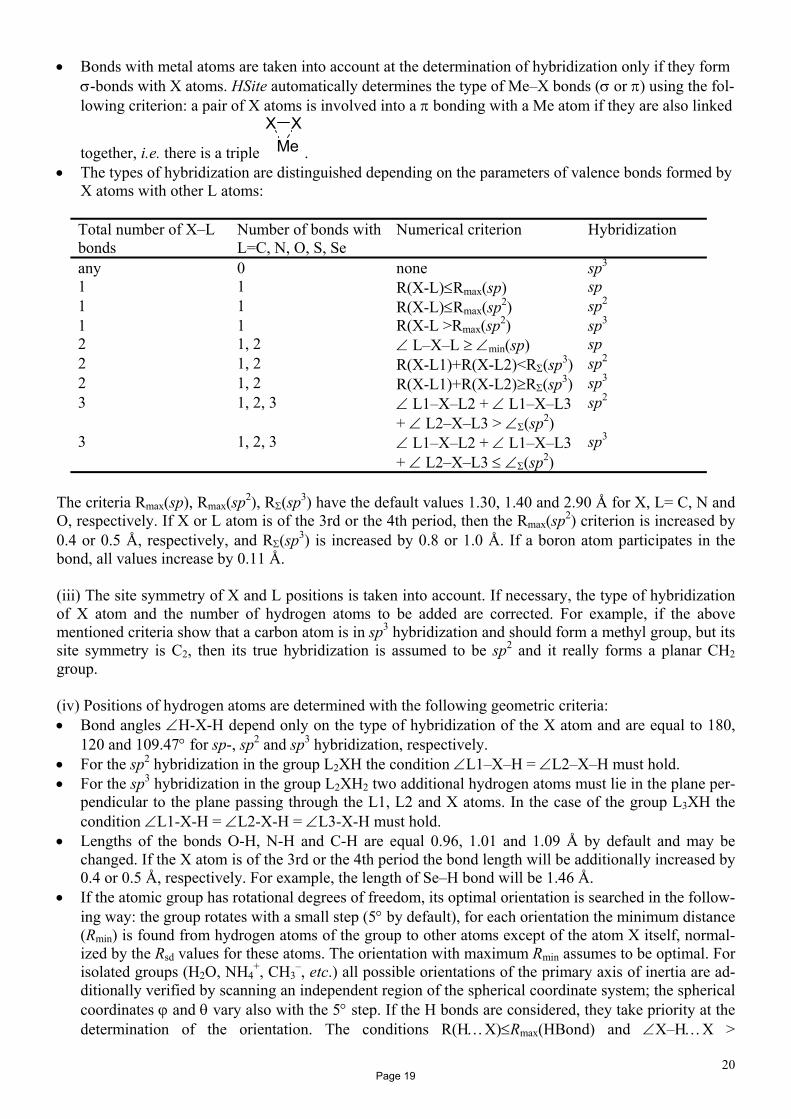


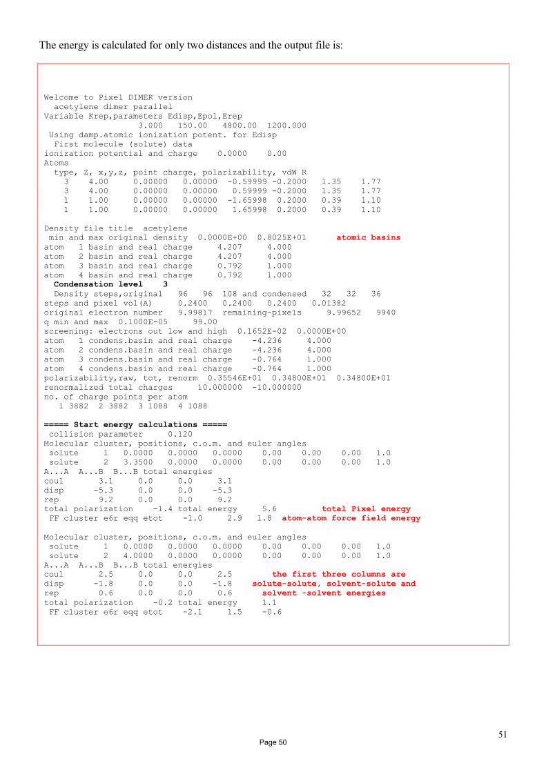


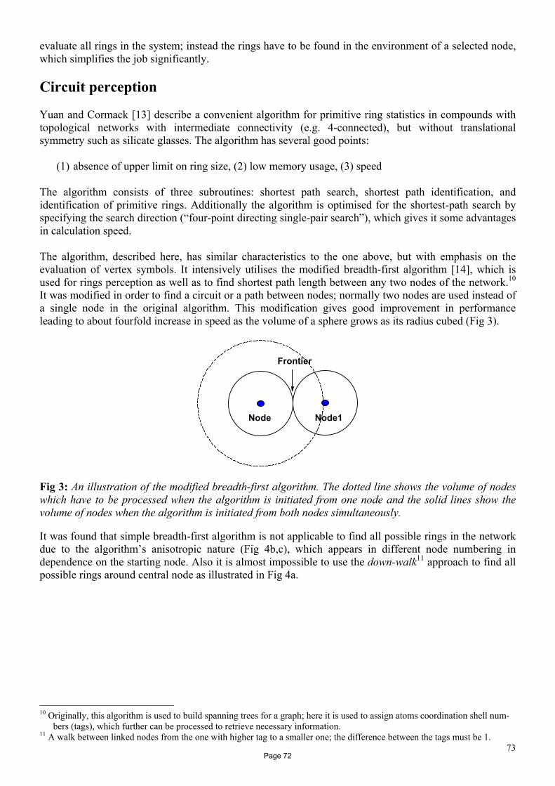


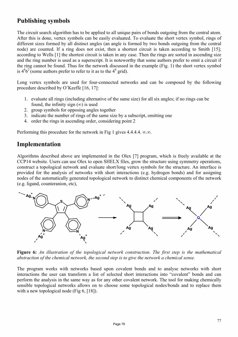


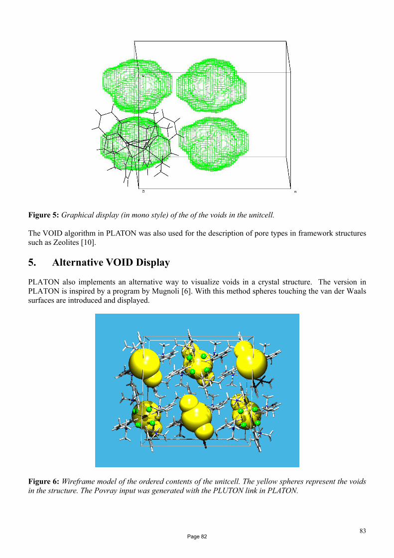

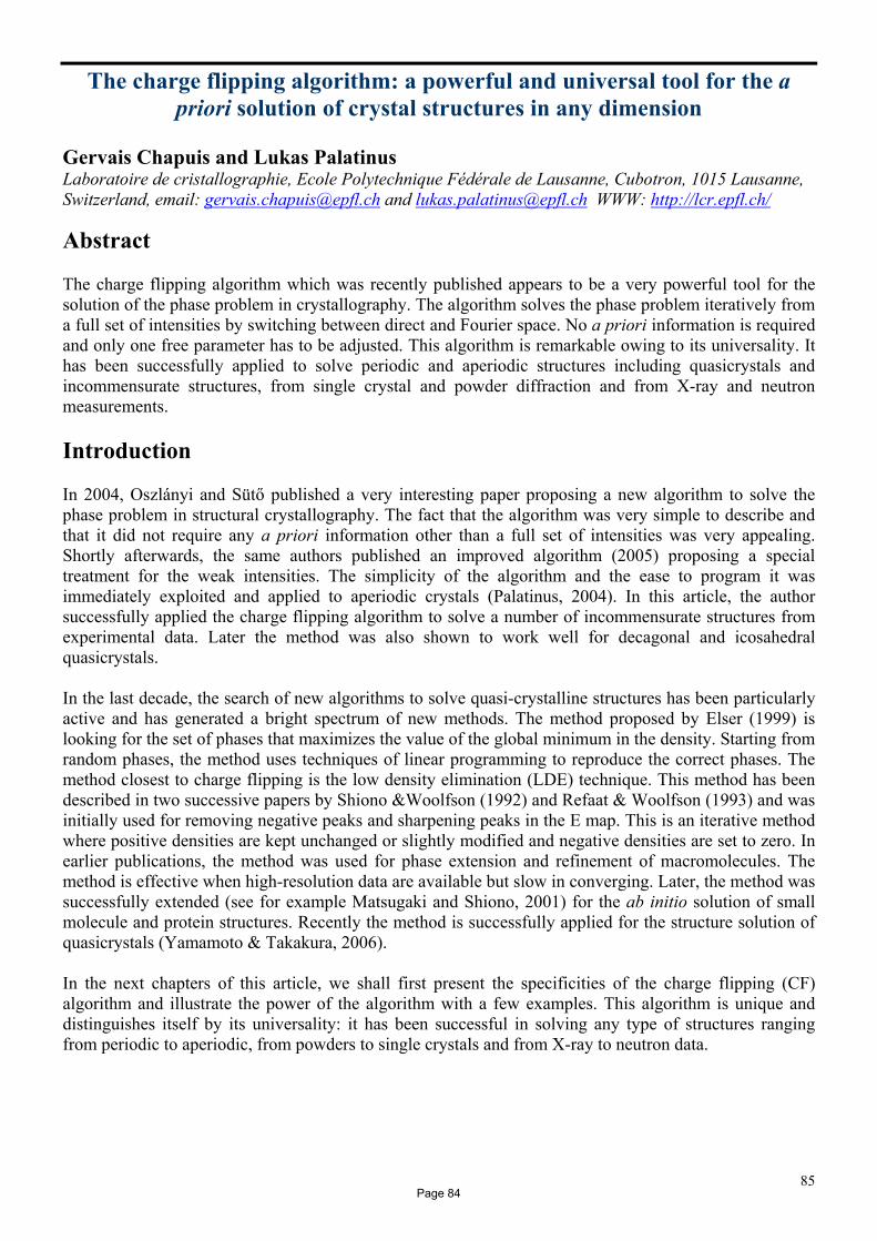


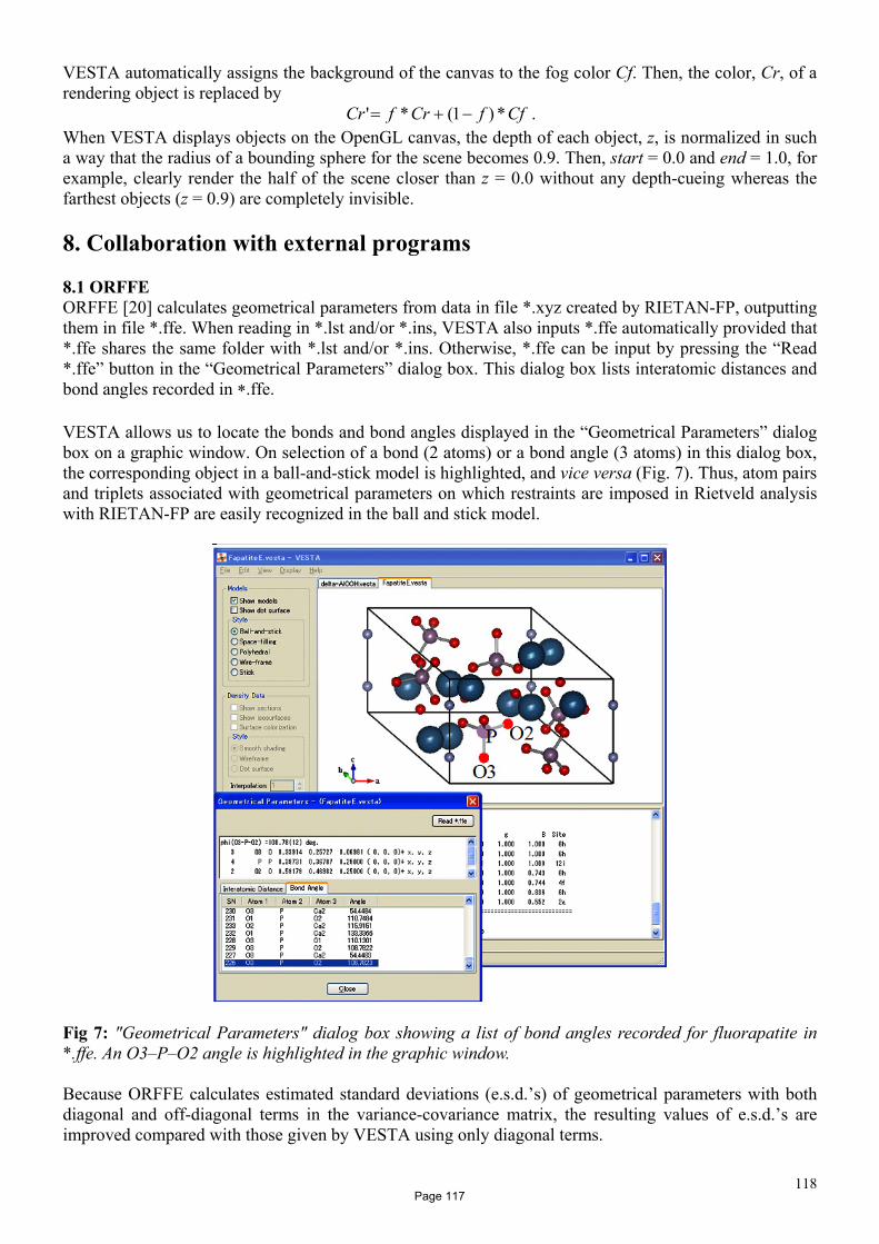


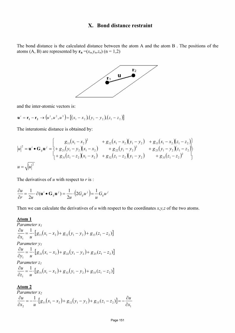


![Crystallographic relations in the Fe[bond]Zn system · Crystallographic Relations in the Fe-Zn System The crystallographic relations between the various Fe-Zn compounds have been](https://img.pdfslide.net/doc/110x75/5f0570af7e708231d412f970/crystallographic-relations-in-the-febondzn-system-crystallographic-relations-in.jpg)