Embed Size (px)
Citation preview
Computers & Industrial Engineering 63 (2012) 223–234
Contents lists available at SciVerse ScienceDirect
Computers & Industrial Engineering
journal homepage: www.elsevier .com/ locate/caie
Common due date assignment and scheduling with a rate-modifying activityto minimize the due date, earliness, tardiness, holding, and batch delivery cost q
Yunqiang Yin a,b, T.C.E. Cheng c, Dehua Xu a,b, Chin-Chia Wu d,⇑a State Key Laboratory Breeding Base of Nuclear Resources and Environment, East China Institute of Technology, Nanchang 330013, Chinab School of Sciences, East China Institute of Technology, Fuzhou, Jiangxi 344000, Chinac Department of Logistics and Maritime Studies, The Hong Kong Polytechnic University, Hung Hom, Kowloon, Hong Kongd Department of Statistics, Feng Chia University, Taichung, Taiwan
a r t i c l e i n f o a b s t r a c t
Article history:Received 30 October 2011Received in revised form 29 January 2012Accepted 22 February 2012Available online 6 March 2012
Keywords:SchedulingDue date assignmentBatch deliveryRate-modifying activity
0360-8352/$ - see front matter � 2012 Elsevier Ltd. Adoi:10.1016/j.cie.2012.02.015
q This manuscript was processed by Area Editor Ha⇑ Corresponding author.
E-mail address: [email protected] (C.-C. Wu).
We consider a single-machine batch delivery scheduling and common due date assignment problem. Inaddition to making decisions on sequencing the jobs, determining the common due date, and schedulingjob delivery, we consider the option of performing a rate-modifying activity on the machine. The process-ing time of a job scheduled after the rate-modifying activity decreases depending on a job-dependent fac-tor. Finished jobs are delivered in batches. There is no capacity limit on each delivery batch, and the costper batch delivery is fixed and independent of the number of jobs in the batch. The objective is to find acommon due date for all the jobs, a location of the rate-modifying activity, and a delivery date for eachjob to minimize the sum of earliness, tardiness, holding, due date, and delivery cost. We provide someproperties of the optimal schedule for the problem and present polynomial algorithms for some specialcases.
� 2012 Elsevier Ltd. All rights reserved.
1. Introduction
Meeting due dates is among the most important goals of sched-uling. There are many practical situations in which a common duedate exists, e.g. in just-in-time production, in assembly scheduling,or in batch delivery. Furthermore, it might be reasonable to assigna common due date to a set of jobs to treat different customersequally. Generally, two situations of due date determinationshould be distinguished: (i) the common due date is (externally)given or agreed upon and (ii) the common due date is determined(internally) by the company. The latter situation corresponds to thesystem in which, for some reason (e.g., appointment, technical con-straints, etc.), several tasks are to be completed at the same time,e.g., several jobs from the same customer form a single order orthe components of a product should be ready by the same timefor assembly. In chemical and food production, the common duedate model applies if some of the involved substances or compo-nents have a limited life span (a ‘‘best before’’ time), which im-poses a common due date on the whole mixture or the finalproduct. There are many papers that focus on the common duedate assignment problem (e.g., Adamopoulos & Pappis, 1995;Birman & Mosheiov, 2004; Biskup & Jahnke, 2001; Cheng, 1984,
ll rights reserved.
ns Kellerer.
1987, 1989; Cheng, Chen, & Shakhlevich, 2002, 2004, 2007; De,Ghosh, & Wells, 1991; Gordon & Strusevich, 2009; Hsu, Yang, &Yang, 2011; Kahlbacher & Cheng, 1993; Li, Ng, & Yuan, 2011;Min & Cheng, 2006; Mosheiov, 2001; Mosheiov & Yovel, 2006;Ng, Cheng, Kovalyov, & Lam, 2003; Panwalkar, Smith, & Seidmann,1982; Shabtay & Steiner, 2006). For state-of-the-art reviews ofscheduling models considering common due date assignment, aswell as practical applications of such models, the reader may referto Cheng and Gupta (1989), Gordon, Proth, and Chu (2002, 2010),and Lauff and Werner (2004).
All of the above papers treat the delivery cost as either negligi-ble or irrelevant. In other words, they focus on the machine sched-uling problem, while ignoring the problem of scheduling thedeliveries of the finished jobs. However, delivery cost is a signifi-cant cost element in production, whereby the production cost de-pends not only on when jobs are processed but also when finishedjobs are delivered. Thus, as observed by Hermann and Lee (1993), arealistic production scheduling model should include scheduling ofboth job processing and job delivery. Several earlier papers haveconsidered scheduling models with both job processing and jobdelivery. Cheng and Kahlbacher (1993) show that the batch deliv-ery problem to minimize the sum of weighted earliness penaltyand delivery cost is NP-hard, while the case with equal weightsis polynomially solvable. Cheng and Gordon (1994) provide apseudopolynomial dynamic programming algorithm to solve theproblem and show that the case with identical processing timesis also polynomially solvable. Hermann and Lee (1993) study
224 Y. Yin et al. / Computers & Industrial Engineering 63 (2012) 223–234
another batch delivery problem, where all the jobs have a givenrestrictive common due date. The objective is to minimize thesum of earliness penalty, tardiness penalty, and delivery cost. Theyprovide a pseudopolynomial dynamic programming algorithm tosolve the problem. Chen (1996) studies a variant of the problemintroduced by Hermann and Lee (1993) where the common duedate is not given but a decision variable to be determined, andshows that the problem can be solved in O(n5) time. Both Hermannand Lee (1993) and Chen (1996) assume that all the early jobs aredelivered on time to the customer without any cost, ignoring thepossibility that early jobs may be delivered in batches. Shabtay(2010) addresses a single-machine scheduling problem similar tothe one studied by Hermann and Lee (1993), where each job is as-signed a due date without restrictions. He applies the best deliverystrategy to all the jobs (not only to the tardy ones), includes theearliness penalty in the objective function and considers the caseof acceptable lead-time. He shows that the problem is NP-hardand presents a polynomial-time solution algorithm for two specialcases. Yin, Cheng, Hsu, and Wu (submitted for publication) study avariant of the problem investigated by Chen (1996) by replacingthe common due date assumption with a common due windowassumption and by allowing the delivering of the early jobs inmore than one batch in the objective function. They show thatthe problem can be optimally solved in O(n8) time and that somespecial cases of the problem can be optimally solved by lower or-der algorithms.
In this paper we extend the problem studied by Chen (1996) tothe cases where holding cost is included in the objective functionand an additional rate-modifying activity is allowed. This activityrequires a fixed time interval during which the machine is turnedoff and production stops. On the other hand, after the rate-modify-ing activity, the machine becomes more efficient, so the jobs pro-cessed after the activity have shortened processing times.Scheduling a rate-modifying activity becomes a popular topicamong researchers in the last decade. Lee and Leon (2001) studyseveral single-machine scheduling problems in this class to mini-mize the makespan, flowtime, weighted flowtime, and maximumlateness. Lodree and Geiger (2010) investigate scheduling with arate-modifying activity under the assumption that a job’s process-ing time is time-dependent. For the sequence-independent, single-machine makespan problem with position-dependent processingtimes, they prove that under certain conditions, the optimal policyis to schedule the rate-modifying activity in the middle of the jobsequence. Mosheiov and Sidney (2004) study the problems to min-imize the makespan with precedence relations, the makespan withlearning effects, and the number of tardy jobs. Mosheiov and Oron(2006) consider common due date assignment and single-machinescheduling with the possibility of performing a rate-modifyingactivity on the machine that changes the processing times of thejobs scheduled after the activity. The objective is to minimize thetotal weighted sum of earliness, tardiness, and due date cost. Theyprovide an (O(n4)) algorithm to solve the problem. Gordon and Tar-asevich (2009) further address the problem studied in Mosheiovand Oron (2006). They provide several properties of the problem,which in some cases reduce the complexity of the solution algo-rithm. Zhao, Tang, and Cheng (2009) consider parallel-machinescheduling with rate-modifying activities. For the problem to min-imize the total completion time, they provide a polynomial algo-rithm to solve it. For the problem to minimize the weightedcompletion time, they provide a pseudopolynomial dynamic pro-gramming algorithm to solve the case where the jobs satisfy anagreeable condition. Wang and Wang (2010) consider single-ma-chine scheduling with assignable slack (SLK) due dates and arate-modifying activity to minimize the total earliness, tardiness,and common flow allowance cost. They give a polynomial-timesolution for the problem. Yin, Cheng, Wu, and Cheng (submitted
for publication) study a problem similar to that studied in this pa-per with a different objective of finding a common due date for allthe jobs, a location of the rate-modifying activity, and a deliverydate for each job to minimize the sum of earliness cost, weightednumber of tardy jobs, holding cost, due date penalty, and deliverycost. Under the assumption that the earliness and holding costs areproportional to their corresponding durations, they investigate thestructural properties of the optimal schedule of the problem andpresent polynomial algorithms for three special cases.
Our problem considered in this paper includes scheduling deci-sions on (i) the job sequence, (ii) the common due date, (iii) therate-modifying activity, and (iv) the delivery date for each job, soas to minimize the sum of earliness, tardiness, holding cost, duedate, and delivery cost. The rest of the paper is organized as fol-lows: In Section 2 we introduce and formulate the problem. In Sec-tion 3 we provide some properties of the optimal schedule. InSection 4 we develop polynomial algorithms for some special casesof the problem. We conclude the paper and suggest some topics forfuture research in the last section.
2. Model formulation
In this section we first introduce the notation to be usedthroughout the paper, followed by formulation of the problem.
n
The number of jobs (n P 2) pj The processing time of job Jjd
The common due date to bedetermined for all the jobs, i.e., dj = dwj
The modifying rate of job Jj(0 < wj 6 1)
Cj The completion time of job JjDj
The delivery time of job Jj (Dj P Cj) Ej = max{0,d � Dj} The earliness of job JjTj = max{0,Dj � d}
The tardiness of job JjHj = Dj � Cj
The holding time of job Jj, which is thetime between the moment the jobfinishes its processing and themoment it is delivereda
The unit cost of earliness b The unit cost of tardiness c The unit due date assignment cost h The unit cost of holding a job d The constant batch delivery costwhere j = 1, 2, . . . , n. In what follows, given any sequence S, we usethe subscript [j] to denote the job in position j of sequence S.
Assume that there is a set of independent jobs N = {J1, J2, . . . , Jn} tobe processed on a single machine. The machine can handle at mostone job at a time and job preemption is not allowed. All the jobs areavailable for processing at time zero. The jobs are to be delivered inbatches to customers. We assume that there is no capacity limit oneach batch delivery and that the cost per delivery is fixed, i.e., thecost is independent of the number of jobs delivered in a batch.Hence, it may be beneficial to delay the shipping of a job until thedelivery time of the next job because the delay saves a deliverycharge. The scheduler also has an option to perform a rate-modify-ing activity on the machine. The rate-modifying activity is denotedby rm, and the starting time and the length of rm are denoted by srm
and t, respectively. When the machine is undergoing rm, no produc-tion is possible. The processing time of job Jj is pj if the job is pro-cessed prior to rm, and wjpj if it is scheduled after it, j = 1, 2, . . . , n.The objective is to determine (i) the job sequence, (ii) the commondue date for all the jobs, (iii) the time (location) to schedule the
Y. Yin et al. / Computers & Industrial Engineering 63 (2012) 223–234 225
rate-modifying activity, (iv) the number of delivery batches, m, and(v) the partition of the job sequence into m batches,B = (B1,B2, . . . ,Bm), such that the following objective function isminimized:
ZðS;d; rm;BÞ ¼Xn
j¼1
ðaEj þ bTj þ hHj þ cdÞ þ dm; ð1Þ
where h 6min{a,b}. The condition h 6min{a,b}, assumed in Shab-tay (2010), is reasonable because earliness and tardiness affect cus-tomers more than holding finished jobs in stock. We say that a job Jj
is early if Cj 6 d; otherwise, it is tardy. It is easy to see that each jobJj should be delivered at its completion time, i.e., Dj = Cj, or at thecompletion time of some other job Jk processed after Jj, i.e.,Dj = Ck > Cj. We use Bkto denote the set of jobs contained in thekth tardy batch (k = 1,2, . . .). Each job in Bi is scheduled before allthe jobs in Bj if i < j. It can easily be shown that each batch Bk is aset of consecutive jobs and its delivery date is the completion timeof the last job in it. Using the conventional notation for describingscheduling problems, we denote the problem under study as1jrm;B;CONj
Pnj¼1ðaEj þ bTj þ hHj þ cdÞ þ dm.
3. Preliminary analysis
In this section we introduce some basic properties about thestructure of an optimal schedule for the problem 1jrm;B;CONj
Pnj¼1 ðaEj þ bTj þ hHj þ cdÞ þ dm.
Lemma 3.1. For the problem 1jrm;B;CONjPn
j¼1ðaEj þ bTj þ hHj
þcdÞ þ dm, there exists an optimal schedule that satisfies the follow-ing properties:
(1) the jobs are processed continuously from time 0 or t withoutany idle time except the rate-modifying activity.
(2) the optimal due date is either 0 or t or the delivery date of somebatch.
Proof. The proof of (1) is obvious and omitted. We prove (2). Sup-pose that S is an optimal schedule and the jobs in S are partitionedinto m batches fJ½1�; . . . ; J½l1 �g, fJ½l1þ1�; . . . ; J½l2 �g; . . . ; andfJ½lm�1þ1�; � � � ; J½lm �g with lm = n in which the common due date d isnot 0, t, nor the delivery date of any batch. By (1), we can supposethat jobs in S are processed continuously without any idle timeexcept the rate-modifying activity. We split the proof into the fol-lowing two cases.
Case 1: d > C[n]. Then each job is early. Consider decreasing d byan amount D = d � C[n] > 0. Then the decrease in theobjective value is n(a + c)(d � C[n]), which is positive.
Case 2: C½lk�1 � < d < C½lk � for some k = 1, 2, . . . , n � 1. Suppose thatalk�1 + nc 6 b(n � lk�1). Consider increasing d by anamount D ¼ C½lk � � d > 0. Then the decrease in the objec-tive value is (�alk�1 � nc + b(n � lk�1))D, which is non-negative. On the other hand, suppose thatalk�1 + nc > b(n � lk�1). Consider reducing d by anamount D ¼ d� Clk�1
> 0. Then the decrease in theobjective value is (alk�1 + nc � b(n � lk�1))D, which isnegative. If the number of batches before batch Bk is 0,i.e., lk�1 = 0, then d may be equal to 0 or t.
Therefore, in both cases, we can find a schedule with property(2) that is better than S, as required. h
Lemma 3.1 indicates that the jobs in any batch are either allearly or all tardy. We call the batch containing only early jobs anearly batch and the batch containing only tardy jobs a tardy batch.
Now given an arbitrary fixed job sequence {J[1], J[2], . . . , J[n]} thatsatisfies Lemma 3.1, assume that the job sequence is partitionedinto m batches B1 ¼ fJ½1�; . . . ; J½l1 �g, B2 ¼ fJ½l1þ1�; . . . ; J½l2 �g; . . ., andBm ¼ fJ½lm�1þ1�; . . . ; J½lm �g, where li denotes the number of jobs in thefirst i batches for i = 1, 2, . . . , m, with l0 = 0 and lm = n, soDj ¼
Plik¼1p½k� for j 2 fJ½li�1þ1�; . . . ; J½li �g and i = 1, 2, . . . , m. Denote the
number of jobs in Bk by jBkj. Let u denote the index of the batchwhose delivery date coincides with the common due date withu = 0, 1, . . . , m, and v denote the position of the job just beforewhich the rate-modifying activity is performed with v = 1, 2, . . . ,n + 1, where u = 0 means that the number of early jobs is 0 andv = n + 1 denotes that the rate-modifying activity is not performed.Next we analyze the problem for given positions of the commondue date and the rate-modifying activity.
Lemma 3.2. Given values of u and v, the objective (1) can bere-formulated as
ZðS; d; rm;BÞ ¼ n minfb; cgt þ bXm
k¼1
ðn� lk�1ÞXlk
j¼lk�1þ1
w½j�p½j�
þ hXm
k¼1
Xlk
j¼lk�1þ1
ðj� 1� lk�1Þw½j�p½j�
0@
1Aþmd; ð2Þ
if u = 0 and v = 1;
ZðS; d; rm;BÞ ¼Xu
k¼1
ðalk�1 þ ncÞPk þ ðals�1 þ ncþ v � ls�1 � 1Þt
þ bXm
k¼uþ1
ðn� lk�1ÞPk þ hXs�1
k¼1
Xlk
j¼lk�1þ1
ðj� 1� lk�1Þp½j�
0@
þXv�1
j¼ls�1þ1
ðj� 1� lk�1Þp½j� þXls
j¼vðj� 1� lk�1Þw½j�p½j�
þXm
k¼sþ1
Xlk
j¼lk�1þ1
ðj� 1� lk�1Þw½j�p½j�
1Aþmd; ð3Þ
if ls�1 < v 6 ls (1 6 s 6 u);
ZðS; d; rm;BÞ ¼Xu
k¼1
ðalk�1 þ ncÞXlk
j¼lk�1þ1
p½j� þ bXm
k¼uþ1
ðn� lk�1Þ
Xlk
j¼lk�1þ1
p½j� þ hXm
k¼1
Xlk
j¼lk�1þ1
ðj� 1� lk�1Þp½j�
0@
1Aþmd;
ð4Þ
if v = n + 1; and
ZðS; d; rm;BÞ ¼Xu
k¼1
ðalk�1 þ ncÞPk þ ðbðn� ls�1Þ þ v � ls�1 � 1Þt
þ bXm
k¼uþ1
ðn� lk�1ÞPk þ hXs�1
k¼1
Xlk
j¼lk�1þ1
ðj� 1� lk�1Þp½j�
0@
þXv�1
j¼ls�1þ1
ðj� 1� lk�1Þp½j� þXls
j¼vðj� 1� lk�1Þw½j�p½j�
þXm
k¼sþ1
Xlk
j¼lk�1þ1
ðj� 1� lk�1Þw½j�p½j�
1Aþmd;
if ls�1 < v 6 ls (u < s 6m), where Pk denotes the total processing time ofthe jobs in batch Bk, i.e.
226 Y. Yin et al. / Computers & Industrial Engineering 63 (2012) 223–234
Pk ¼
Plkj¼lk�1þ1
p½j� k ¼ 1; . . . ; s� 1;
Pv�1
j¼ls�1þ1p½j� þ
Plsj¼v
w½j�p½j� k ¼ s;
Plkj¼lk�1þ1
w½j�p½j� k ¼ sþ 1; . . . ; m:
8>>>>>>>>><>>>>>>>>>:
Proof. We only prove the result for the case ls�1 < v 6 ls (1 6 s 6 u).The other cases can be similarly proved. By Eq. (1), we have
ZðS;d; rm;BÞ ¼Xm
k¼1
jBkjða maxf0;Clu � Clkg þ b maxf0; Clk � ClugÞ
þ hXn
j¼1
ðDj � CjÞ þ ncClu þmd;
¼aXs�1
k¼1
jBkjXv�1
j¼lkþ1
p½j� þ tþXlu
j¼vw½j�p½j�
0@
1Aþa
Xu�1
k¼s
jBkjXlu
j¼lkþ1
w½j�p½j�
0@
1A
þbXm
k¼uþ1
jBkjXlk
j¼luþ1
w½j�p½j�
!þh
Xs�1
k¼1
Xlk
j¼lk�1þ1
ðj�1� lk�1Þp½j�
0@
þðv� ls�1�1ÞtþXv�1
j¼ls�1þ1
ðj�1� lk�1Þp½j� þXls
j¼vðj�1� lk�1Þw½j�p½j�
þXm
k¼sþ1
Xlk
j¼lk�1þ1
ðj�1� lk�1Þw½j�p½j�
1Aþnc
Xv�1
j¼1
p½j� þ tþXlu
j¼vw½j�p½j�
!þmd;
¼Xs�1
k¼1
ðalk�1þncÞXlk
j¼lk�1þ1
p½j�
0@
1Aþðals�1þcÞ
Xv�1
j¼ls�1þ1
p½j� þ tþXls
j¼vw½j�p½j�
!
þXu
k¼sþ1
ðalk�1þncÞXlk
j¼lk�1þ1
w½j�p½j�
0@
1Aþb
Xm
k¼uþ1
ðn� lk�1ÞXlk
j¼lk�1þ1
w½j�p½j�
0@
1A
þhXs�1
k¼1
Xlk
j¼lk�1þ1
ðj�1� lk�1Þp½j� þ ðv� ls�1�1ÞtþXv�1
j¼ls�1þ1
ðj�1� lk�1Þp½j�
0@
þXls
j¼vðj�1� lk�1Þw½j�p½j� þ
Xm
k¼sþ1
Xlk
j¼lk�1þ1
ðj�1� lk�1Þw½j�p½j�Þþmd:
By simple algebra, we obtain the result. h
As a consequence of Lemma 3.2, we have the following result.
Lemma 3.3. Given values of u and v,
(1) the objective value of the problem is minimized if s = 1 andv = ls�1 + 1, i.e., performing the rate-modifying activity at time0, under the condition that ls�1 < v 6 ls and 1 6 s 6 u.
(2) the objective value of the problem will decrease if the rate-mod-ifying activity is performed just before the first job in sometardy batch, under the condition that ls�1 < v 6 ls and u < s 6m.
Proof. We only prove (1). (2) can be similarly proved. Assume thatls�1 < v 6 ls and 1 6 s 6 u for given values of u and v. Firstly, for agiven value of s, it follows from Eq. (3) that the difference betweenthe objective values of the two cases, where v = ls�1 + 1 andls�1 + 1 < v = v0 6 ls is
D ¼Xv 0�1
ðj� 1� lk�1Þðw½j� � 1Þp½j� 6 0;
j¼ls�1þ1implying that performing the rate-modifying activity just before thefist job of some early batch, i.e., v ¼ l0s�1 þ 1 for some s0 such that1 6 s0 6 u, will decrease the objective value. Next, assume that therate-modifying activity is performed before the first job of someearly batch s, then it follows from Eq. (3) that the difference be-tween the objective values of the two cases where s = 1 and1 < s = s0 6 u is D ¼ �als0�1t < 0; as required. h
The next result gives a property of the early batches.
Lemma 3.4. For the problem 1jrm;B;CONjPn
j¼1ðaEj þ bTj þ hHj
þcdÞ þ dm, there exists an optimal schedule in which there is at mostone early batch.
Proof. Suppose that there exists an optimal schedule S satisfyingLemma 3.1 that has at least two early batches Bk ¼ fJ½lk�1þ1�;
J½lk�1þ2�; . . . ; J½lk �g and Bkþ1 ¼ fJ½lkþ1�; J½lkþ2�; . . . ; J½lkþ1 �g. Now consider anew schedule S0 constructed by combining batches Bk and Bk+1 intoone batch fJ½lk�1þ1�; J½lk�1þ2�; . . . ; J½lk �; J½lkþ1�; J½lkþ2�; . . . ; J½lkþ1 �g. By Eq. (5),the difference between the objective values of schedules S0 and S is
D¼alk�1ðPkðSÞþPkþ1ðSÞÞ�alk�1PkðSÞ�alkPkþ1ðSÞþhjBkjPkþ1ðSÞ�d
¼ðh�aÞjBkjPkþ1ðSÞ�d:
Since h 6 a, we have D < 0. Therefore, S0 is a better schedulethan S. Repeating this combining argument for the early batchesyields the result. h
By Lemmas 3.2–2.4, we have the following result.
Lemma 3.5. For the problem 1jrm;B;CONjPn
j¼1ðaEj þ bTj þ hHj
þcdÞ þ dm, it is optimal to perform the rate-modifying activity eitherjust before the first job or just before the first job in some tardy batchin any schedule.
As a consequence of Lemma 3.4, the common due date d equalseither to 0 or t, or it coincides with the delivery date of the firstbatch (the early batch). By Lemma 3.5, we only need to considerthe cases where v = li + 1 (i = 0,1,2, . . . ,m). So Eqs. (2)–(5) can bere-formulated as
ZðS;d;rm;BÞ¼
nminfc;dgtþbPm
k¼uþ1ðn� lk�1ÞPkþmd
þhPmk¼1
Plkj¼lk�1þ1
ðj� lk�1�1Þw½j�p½j� if u¼0 and v ¼1;
ncðPuþ tÞþbPm
k¼uþ1ðn� lk�1ÞPkþmd
þhPmk¼1
Plkj¼lk�1þ1
ðj� lk�1�1Þw½j�p½j� if u¼1 and v ¼1;
ncPuþbPm
k¼uþ1ðn� lk�1ÞPkþbðn� liÞtþmd
þhPi
k¼1
Plkj¼lk�1þ1
ðj� lk�1�1Þp½j�
þPm
k¼iþ1
Plkj¼lk�1þ1
ðj� lk�1�1Þw½j�p½j�
!if v ¼ liþ1ði P 1Þ;
8>>>>>>>>>>>>>>>>>>>>>>>>>>>>><>>>>>>>>>>>>>>>>>>>>>>>>>>>>>:
ð6Þwhere u = 0 or u = 1 and
Pk ¼
Plkj¼lk�1þ1
p½j�; if lk < v;
Plkj¼lk�1þ1
w½j�p½j�; if v 6 lk;
8>>>><>>>>:
k ¼ 1; 2; . . . ; m:
As a consequence of Lemmas 3.1 and 3.5, we can restrict ourattention to schedules without idle times except the rate-modify-ing activity and search for the optimal schedule only among
Y. Yin et al. / Computers & Industrial Engineering 63 (2012) 223–234 227
schedules in which the optimal due date is either 0 or t, or coin-cides with the delivery date of the first batch (the early batch),and the optimal time for the rate-modifying activity is either 0 orthe starting time of the first job in some tardy batch.
The following result presents the optimal properties of the jobsin any batch.
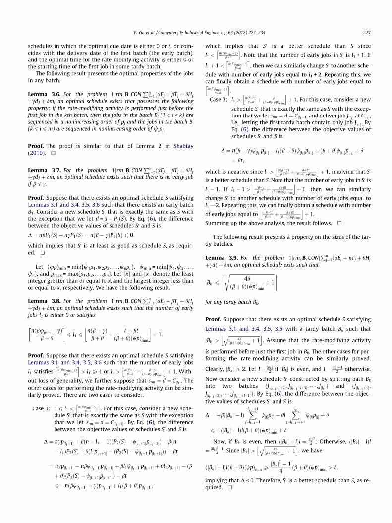
Lemma 3.6. For the problem 1jrm;B;CONjPn
j¼1ðaEj þ bTj þ hHj
þcdÞ þ dm, an optimal schedule exists that possesses the followingproperty: if the rate-modifying activity is performed just before thefirst job in the kth batch, then the jobs in the batch Bi (1 6 i < k) aresequenced in a nonincreasing order of pj and the jobs in the batch Bi
(k 6 i 6m) are sequenced in nonincreasing order of wjpj.
Proof. The proof is similar to that of Lemma 2 in Shabtay(2010). h
Lemma 3.7. For the problem 1jrm;B;CONjPn
j¼1ðaEj þ bTj þ hHj
þcdÞ þ dm, an optimal schedule exists such that there is no early jobif b 6 c.
Proof. Suppose that there exists an optimal schedule S satisfyingLemmas 3.1 and 3.4, 3.5, 3.6 such that there exists an early batchB1. Consider a new schedule S0 that is exactly the same as S withthe exception that we let d = d � P1(S). By Eq. (6), the differencebetween the objective values of schedules S0 and S is
D ¼ nbP1ðSÞ � ncP1ðSÞ ¼ nðb� cÞP1ðSÞ 6 0;
which implies that S0 is at least as good as schedule S, as requir-ed. h
Let (up)min = min{w1p1,w2p2, . . . ,wnpn}, wmin = min{w1,w2, . . . ,wn}, and pmax = max{p1,p2, . . . ,pn}. Let dxe and bxc denote the leastinteger greater than or equal to x, and the largest integer less thanor equal to x, respectively. We have the following result.
Lemma 3.8. For the problem 1jrm;B;CONjPn
j¼1ðaEj þ bTj þ hHj
þcdÞ þ dm, an optimal schedule exists such that the number of earlyjobs l1 is either 0 or satisfies
nðbumin � cÞbþ h
� �6 l1 6
nðb� cÞbþ h
þ dþ btðbþ hÞðwpÞmin
� �þ 1:
Proof. Suppose that there exists an optimal schedule S satisfyingLemmas 3.1 and 3.4, 3.5, 3.6 such that the number of early jobs
l1 satisfies nðbumin�cÞbþh
l m> l1 P 1 or l1 >
nðb�cÞbþh þ
dþbtðbþhÞðwpÞmin
j kþ 1. With-
out loss of generality, we further suppose that srm ¼ d ¼ C½l1 �. Theother cases for performing the rate-modifying activity can be sim-ilarly proved. There are two cases to consider.
Case 1: 1 6 l1 <nðbumin�cÞ
bþh
l m. For this case, consider a new sche-
dule S0 that is exactly the same as S with the exceptionthat we let srm ¼ d ¼ C½l1þ1�. By Eq. (6), the differencebetween the objective values of schedules S0 and S is
D ¼ ncp½l1þ1� þ bðn� l1 � 1ÞðP2ðSÞ � w½l1þ1�p½l1þ1�Þ � bðn� l1ÞP2ðSÞ þ hðl1p½l1þ1� � ðP2ðSÞ � w½l1þ1�p½l1þ1�ÞÞ � bt
¼ ncp½l1þ1� � nbw½l1þ1�p½l1þ1� þ bl1w½l1þ1�p½l1þ1� þ hl1p½l1þ1� � ðbþ hÞðP2ðSÞ � w½l1þ1�p½l1þ1�Þ � bt
6 �nðbw½l1þ1� � cÞp½l1þ1� þ l1ðbþ hÞp½l1þ1�;
which implies that S0 is a better schedule than S since
l1 <nðbumin�cÞ
bþh
l m. Note that the number of early jobs in S0 is l1 + 1. If
l1 þ 1 < nðbumin�cÞbþh
l m, then we can similarly change S0 to another sche-
dule with number of early jobs equal to l1 + 2. Repeating this, wecan finally obtain a schedule with number of early jobs equal to
nðbumin�cÞbþh
l m.
Case 2: l1 >nðb�cÞ
bþh þ dðbþhÞðwpÞmin
j kþ 1. For this case, consider a new
schedule S0 that is exactly the same as S with the excep-tion that we let srm ¼ d ¼ C½l1�1� and deliver job J½l1 � at C½l1 �,i.e., letting the first tardy batch contain only job J½l1 �. ByEq. (6), the difference between the objective values ofschedules S0 and S is
D ¼ nðb� cÞw½l1 �p½l1 � � l1ðbþ hÞw½l1 �p½l1 � þ ðbþ hÞw½l1 �p½l1 � þ d
þ bt;
which is negative since l1 >nðb�cÞ
bþh þdþbt
ðbþhÞðwpÞmin
j kþ 1, implying that S0
is a better schedule than S. Note that the number of early jobs in S0 is
l1 � 1. If l1 � 1 > nðb�cÞbþh þ
dþbtðbþhÞðwpÞmin
j kþ 1, then we can similarly
change S0 to another schedule with number of early jobs equal tol1 � 2. Repeating this, we can finally obtain a schedule with number
of early jobs equal to nðb�cÞbþh þ
dþbtðbþhÞðwpÞmin
j kþ 1.
Summing up the above analysis, the result follows. h
The following result presents a property on the sizes of the tar-dy batches.
Lemma 3.9. For the problem 1jrm;B;CONjPn
j¼1ðaEj þ bTj þ hHj
þcdÞ þ dm, an optimal schedule exits such that
jBkj 6ffiffiffiffiffiffiffiffiffiffiffiffiffiffiffiffiffiffiffiffiffiffiffiffiffiffiffiffiffiffiffiffiffiffiffiffiffiffiffi
4dðbþ hÞðwpÞmin
þ 1
s$ %
for any tardy batch Bk.
Proof. Suppose that there exists an optimal schedule S satisfying
Lemmas 3.1 and 3.4, 3.5, 3.6 with a tardy batch Bk such that
jBkj >ffiffiffiffiffiffiffiffiffiffiffiffiffiffiffiffiffiffiffiffiffiffiffiffiffiffiffiffi
4dðbþhÞðwpÞmin
þ 1qj k
. Assume that the rate-modifying activity
is performed before just the first job in Bk. The other cases for per-forming the rate-modifying activity can be similarly proved.
Clearly, jBkjP 2. Let l ¼ jBk j2 if jBkj is even, and l ¼ jBk j�1
2 otherwise.
Now consider a new schedule S0 constructed by splitting bath Bk
into two batches fJ½lk�1þlþ2�; J½lk�1þlþ3�; � � � ; J½lk �g and fJ½lk�1þ1�;
J½lk�1þ2�; � � � ; J½lk�1þlþ1�g. By Eq. (6), the difference between the objec-tive values of schedules S0 and S is
D ¼ �bðjBkj � lÞXlk�1þl
j¼lk�1þ1
w½j�p½j� � hlXlk
j¼lk�1þlþ1
w½j�p½j� þ d
6 �ðjBkj � lÞlðbþ hÞðwpÞmin þ d:
Now, if Bk is even, then ðjBkj � lÞl ¼ jBk j24 ; Otherwise, ðjBkj � lÞl
¼ jBk j2�14 . Since jBkj >
ffiffiffiffiffiffiffiffiffiffiffiffiffiffiffiffiffiffiffiffiffiffiffiffiffiffiffiffi4d
ðbþhÞðwpÞminþ 1
qj k, we have
ðjBkj � lÞlðbþ hÞðwpÞmin PjBkj2 � 1
4ðbþ hÞðwpÞmin > d;
implying that D < 0. Therefore, S0 is a better schedule than S, as re-quired. h
228 Y. Yin et al. / Computers & Industrial Engineering 63 (2012) 223–234
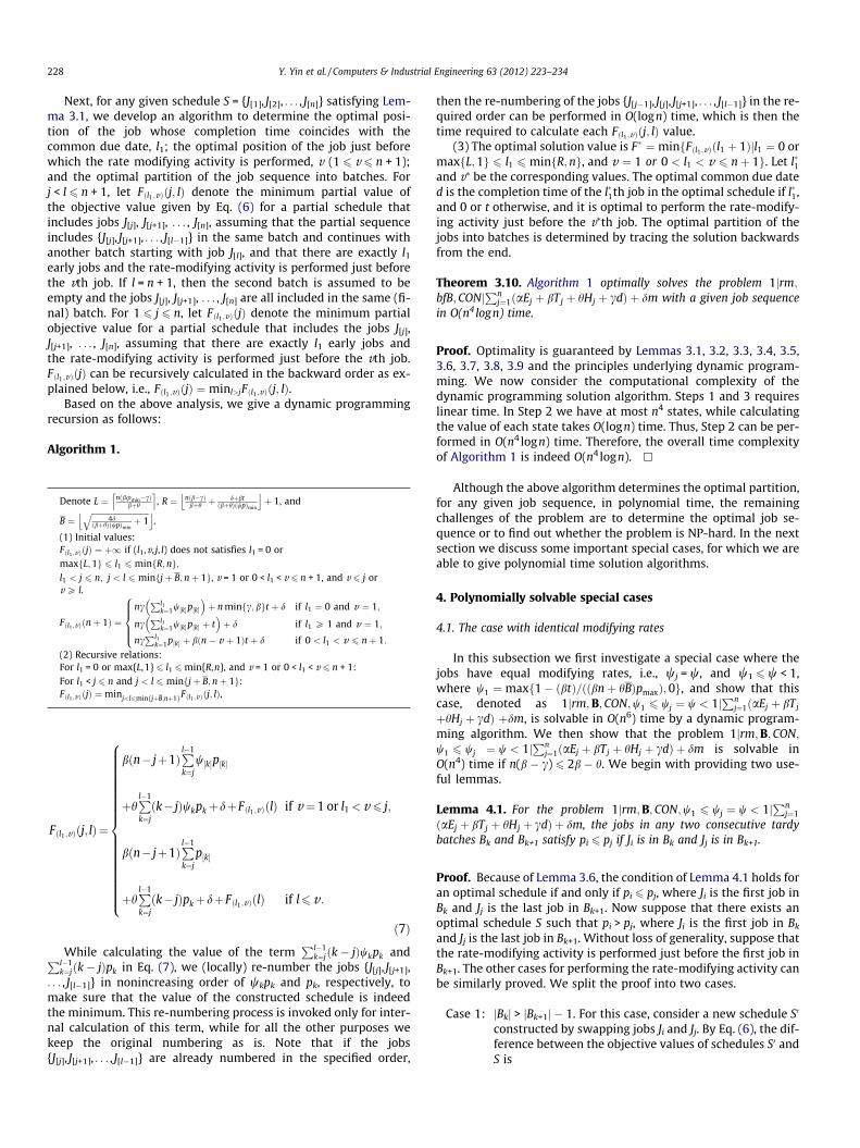
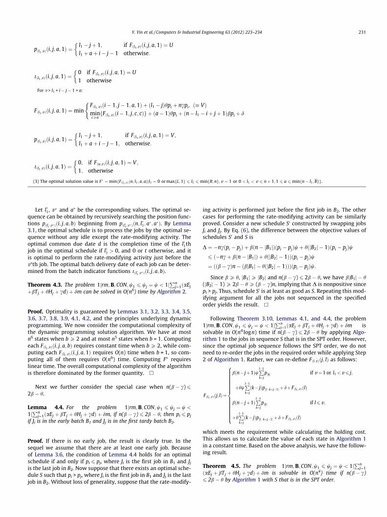
Next, for any given schedule S = {J[1], J[2], . . . , J[n]} satisfying Lem-ma 3.1, we develop an algorithm to determine the optimal posi-tion of the job whose completion time coincides with thecommon due date, l1; the optimal position of the job just beforewhich the rate modifying activity is performed, v (1 6 v 6 n + 1);and the optimal partition of the job sequence into batches. Forj < l 6 n + 1, let Fðl1 ;vÞðj; lÞ denote the minimum partial value ofthe objective value given by Eq. (6) for a partial schedule thatincludes jobs J[j], J[j+1], . . . , J[n], assuming that the partial sequenceincludes {J[j], J[j+1], . . . , J[l�1]} in the same batch and continues withanother batch starting with job J[l], and that there are exactly l1early jobs and the rate-modifying activity is performed just beforethe vth job. If l = n + 1, then the second batch is assumed to beempty and the jobs J[j], J[j+1], . . . , J[n] are all included in the same (fi-nal) batch. For 1 6 j 6 n, let Fðl1 ;vÞðjÞ denote the minimum partialobjective value for a partial schedule that includes the jobs J[j],J[j+1], . . . , J[n], assuming that there are exactly l1 early jobs andthe rate-modifying activity is performed just before the vth job.Fðl1 ;vÞðjÞ can be recursively calculated in the backward order as ex-plained below, i.e., Fðl1 ;vÞðjÞ ¼minl>jFðl1 ;vÞðj; lÞ.
Based on the above analysis, we give a dynamic programmingrecursion as follows:
Algorithm 1.
Denote L ¼ nðbumin�cÞbþh
l m, R ¼ nðb�cÞ
bþh þdþbt
ðbþhÞðwpÞmin
j kþ 1, and
B ¼ffiffiffiffiffiffiffiffiffiffiffiffiffiffiffiffiffiffiffiffiffiffiffiffiffiffiffiffiffi
4dðbþhÞðwpÞmin
þ 1qj k
.
(1) Initial values:Fðl1 ;vÞðjÞ ¼ þ1 if (l1,v, j, l) does not satisfies l1 = 0 ormaxfL;1g 6 l1 6minfR;ng;l1 < j 6 n; j < l 6 minfjþ B;nþ 1g, v = 1 or 0 < l1 < v 6 n + 1, and v 6 j orv P l.
Fðl1 ;vÞðnþ 1Þ ¼nc
Pl1k¼1w½k�p½k�
� �þ n minfc;bgt þ d if l1 ¼ 0 and v ¼ 1;
ncPl1
k¼1w½k�p½k� þ t� �
þ d if l1 P 1 and v ¼ 1;
ncPl1
k¼1p½k� þ bðn� v þ 1Þt þ d if 0 < l1 < v 6 nþ 1:
8>>><>>>:
(2) Recursive relations:For l1 = 0 or max{L,1} 6 l1 6min{R,n}, and v = 1 or 0 < l1 < v 6 n + 1:For l1 < j 6 n and j < l 6 minfjþ B;nþ 1g:Fðl1 ;vÞðjÞ ¼minj<l6minfjþB;nþ1gFðl1 ;vÞðj; lÞ,
Fðl1 ;vÞðj; lÞ¼
bðn� jþ1ÞPl�1
k¼jw½k�p½k�
þhPl�1
k¼jðk� jÞwkpkþdþFðl1 ;vÞðlÞ if v ¼1 or l1 <v 6 j;
bðn� jþ1ÞPl�1
k¼jp½k�
þhPl�1
k¼jðk� jÞpkþdþFðl1 ;vÞðlÞ if l6v:
8>>>>>>>>>>>>>>>>>><>>>>>>>>>>>>>>>>>>:
ð7Þ
While calculating the value of the termPl�1
k¼jðk� jÞwkpk andPl�1k¼jðk� jÞpk in Eq. (7), we (locally) re-number the jobs {J[j], J[j+1],
. . . , J[l�1]} in nonincreasing order of wkpk and pk, respectively, tomake sure that the value of the constructed schedule is indeedthe minimum. This re-numbering process is invoked only for inter-nal calculation of this term, while for all the other purposes wekeep the original numbering as is. Note that if the jobs{J[j], J[j+1], . . . , J[l�1]} are already numbered in the specified order,
then the re-numbering of the jobs {J[j�1], J[j], J[j+1], . . . , J[l�1]} in the re-quired order can be performed in O(logn) time, which is then thetime required to calculate each Fðl1 ;vÞðj; lÞ value.
(3) The optimal solution value is F� ¼minfFðl1 ;vÞðl1 þ 1Þjl1 ¼ 0 ormaxfL;1g 6 l1 6 minfR;ng, and v ¼ 1 or 0 < l1 < v 6 nþ 1g. Let l�1and v⁄ be the corresponding values. The optimal common due dated is the completion time of the l�1th job in the optimal schedule if l�1,and 0 or t otherwise, and it is optimal to perform the rate-modify-ing activity just before the v⁄th job. The optimal partition of thejobs into batches is determined by tracing the solution backwardsfrom the end.
Theorem 3.10. Algorithm 1 optimally solves the problem 1jrm;bfB;CONj
Pnj¼1ðaEj þ bTj þ hHj þ cdÞ þ dm with a given job sequence
in O(n4 logn) time.
Proof. Optimality is guaranteed by Lemmas 3.1, 3.2, 3.3, 3.4, 3.5,3.6, 3.7, 3.8, 3.9 and the principles underlying dynamic program-ming. We now consider the computational complexity of thedynamic programming solution algorithm. Steps 1 and 3 requireslinear time. In Step 2 we have at most n4 states, while calculatingthe value of each state takes O(logn) time. Thus, Step 2 can be per-formed in O(n4 logn) time. Therefore, the overall time complexityof Algorithm 1 is indeed O(n4 logn). h
Although the above algorithm determines the optimal partition,for any given job sequence, in polynomial time, the remainingchallenges of the problem are to determine the optimal job se-quence or to find out whether the problem is NP-hard. In the nextsection we discuss some important special cases, for which we areable to give polynomial time solution algorithms.
4. Polynomially solvable special cases
4.1. The case with identical modifying rates
In this subsection we first investigate a special case where thejobs have equal modifying rates, i.e., wj = w, and w1 6 w < 1,where w1 ¼maxf1� ðbtÞ=ððbnþ hBÞpmaxÞ;0g, and show that thiscase, denoted as 1jrm;B;CON;w1 6 wj ¼ w < 1j
Pnj¼1ðaEj þ bTj
þhHj þ cdÞ þdm, is solvable in O(n6) time by a dynamic program-ming algorithm. We then show that the problem 1jrm;B;CON;w1 6 wj ¼ w < 1j
Pnj¼1ðaEj þ bTj þ hHj þ cdÞ þ dm is solvable in
O(n4) time if n(b � c) 6 2b � h. We begin with providing two use-ful lemmas.
Lemma 4.1. For the problem 1jrm;B;CON;w1 6 wj ¼ w < 1jPn
j¼1ðaEj þ bTj þ hHj þ cdÞ þ dm, the jobs in any two consecutive tardybatches Bk and Bk+1 satisfy pi 6 pj if Ji is in Bk and Jj is in Bk+1.
Proof. Because of Lemma 3.6, the condition of Lemma 4.1 holds foran optimal schedule if and only if pi 6 pj, where Ji is the first job inBk and Jj is the last job in Bk+1. Now suppose that there exists anoptimal schedule S such that pi > pj, where Ji is the first job in Bk
and Jj is the last job in Bk+1. Without loss of generality, suppose thatthe rate-modifying activity is performed just before the first job inBk+1. The other cases for performing the rate-modifying activity canbe similarly proved. We split the proof into two cases.
Case 1: jBkj > jBk+1j � 1. For this case, consider a new schedule S0
constructed by swapping jobs Ji and Jj. By Eq. (6), the dif-ference between the objective values of schedules S0 andS is
Y. Yin et al. / Computers & Industrial Engineering 63 (2012) 223–234 229
D¼ �bðn� lk�1Þðpi�pjÞþbðn� lkÞðpi�pjÞw
þhðjBkþ1j�1Þðpi�pjÞw
6bð�lkþ lk�1Þðpi�pjÞw
þhðjBkþ1j�1Þðpi�pjÞw¼
ðhðjBkþ1j�1Þ�bjBkjÞðpi�pjÞw;
which is negative, since b P h, jBkj > jBk+1j � 1 and pi > pj.
Case 2: jBkj 6 jBk+1j � 1. For this case, consider a new schedule S0constructed by placing job Jj in the last position of Bk. ByEq. (6), the difference between the objective values ofschedules S0 and S is
D¼ bðn� lk�1Þpj�bPkþ1ðSÞ�bðn� lk�1ÞpjwþhjBkjpj
�hðjBkþ1j�1Þpjw�bt
6bnpj�blk�1pjw�bjBkþ1jpjw�bðn� lk�1ÞpjwþhjBkjpj
�hðjBkþ1j�1Þpjw�bt
¼ðbnþhjBkjÞpjð1�wÞþðhþbÞððjBkjþ1Þ� jBkþ1jÞpjw�bt:
Since jBkj 6 B and max 1� btðbnþhBÞpmax
;0n o
6 w, we have (bn + hjBkj)pj(1 � w) 6 bt, implying that D is nonpositive since jBkj 6 jBk+1j � 1.
Thus, in both cases, schedule S0 is at least as good as S. Repeatingthis modifying argument for all the jobs not sequenced in thespecified order yields the result. h
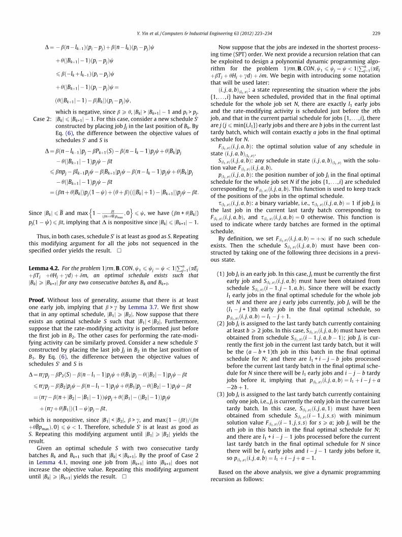
Lemma 4.2. For the problem 1jrm;B;CON;w1 6 wj ¼ w < 1jPn
j¼1ðaEj
þbTj þhHj þ cdÞ þ dm, an optimal schedule exists such thatjBkjP jBk+1j for any two consecutive batches Bk and Bk+1.
Proof. Without loss of generality, assume that there is at leastone early job, implying that b > c by Lemma 3.7. We first showthat in any optimal schedule, jB1jP jB2j. Now suppose that thereexists an optimal schedule S such that jB1j < jB2j. Furthermore,suppose that the rate-modifying activity is performed just beforethe first job in B2. The other cases for performing the rate-modi-fying activity can be similarly proved. Consider a new schedule S0
constructed by placing the last job Jj in B2 in the last position ofB1. By Eq. (6), the difference between the objective values ofschedules S0 and S is
D¼ncpj�bP2ðSÞ�bðn� l1�1ÞpjwþhjB1jpj�hðjB2j�1Þpjw�bt
6ncpj�bjB2jpjw�bðn� l1�1ÞpjwþhjB1jpj�hðjB2j�1Þpjw�bt
¼ðnc�bðnþjB2j� jB1j�1ÞÞwpjþhðjB1j�ðjB2j�1ÞÞpjw
þðncþhjB1jÞð1�wÞpj�bt;
which is nonpositive, since jB1j < jB2j, b > c, and maxf1� ðbtÞ=ðbnþhBpmaxÞ;0g 6 w < 1. Therefore, schedule S0 is at least as good asS. Repeating this modifying argument until jB1jP jB2j yields theresult.
Given an optimal schedule S with two consecutive tardybatches Bk and Bk+1 such that jBkj < jBk+1j. By the proof of Case 2in Lemma 4.1, moving one job from jBk+1j into jBk+1j does notincrease the objective value. Repeating this modifying argumentuntil jBkjP jBk+1j yields the result. h
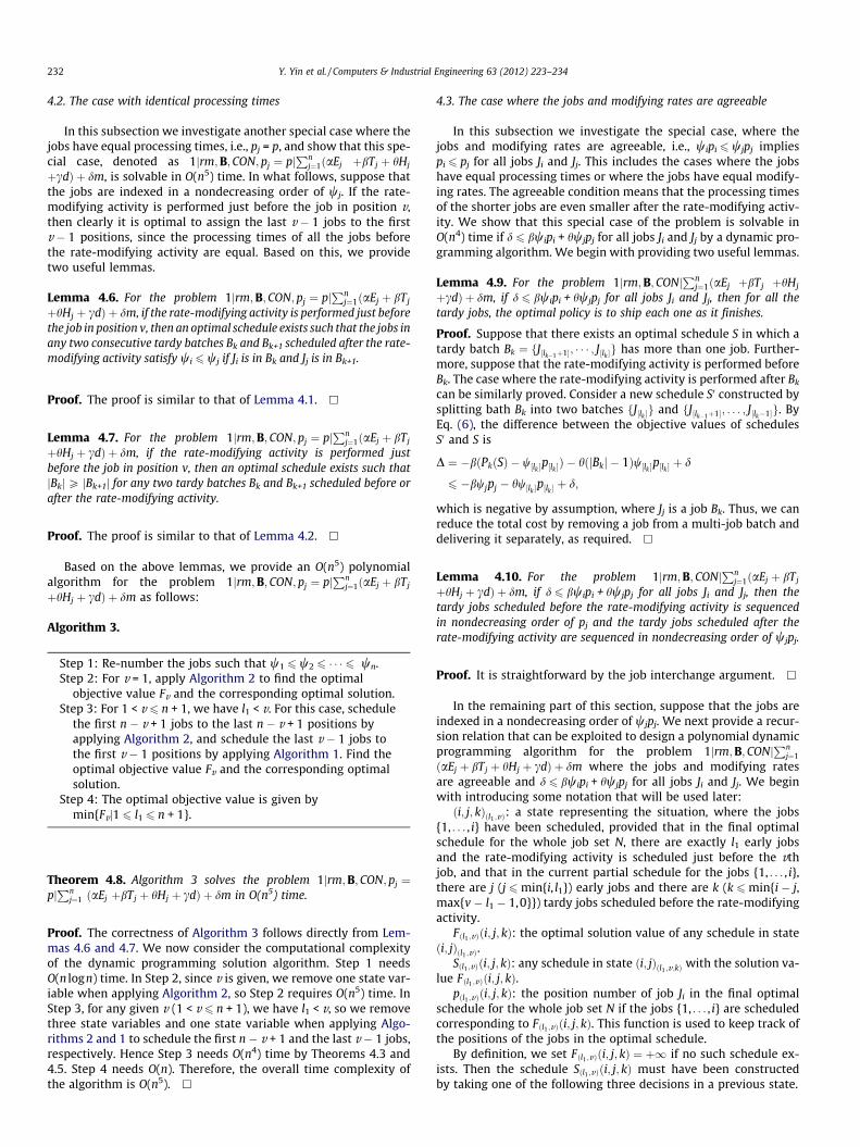
Now suppose that the jobs are indexed in the shortest process-ing time (SPT) order. We next provide a recursion relation that canbe exploited to design a polynomial dynamic programming algo-rithm for the problem 1jrm;B;CON;w1 6 wj ¼ w < 1j
Pnj¼1ðaEj
þbTj þ hHj þ cdÞ þ dm. We begin with introducing some notationthat will be used later:ði; j; a; bÞðl1 ;vÞ: a state representing the situation where the jobs
{1, . . . , i} have been scheduled, provided that in the final optimalschedule for the whole job set N, there are exactly l1 early jobsand the rate-modifying activity is scheduled just before the vthjob, and that in the current partial schedule for jobs {1, . . . , i}, thereare j (j 6min{i, l1}) early jobs and there are b jobs in the current lasttardy batch, which will contain exactly a jobs in the final optimalschedule for N.
Fðl1 ;vÞði; j; a; bÞ: the optimal solution value of any schedule instate ði; j; a; bÞðl1 ;vÞ.
Sðl1 ;vÞði; j; a; bÞ: any schedule in state ði; j; a; bÞðl1 ;vÞ with the solu-tion value Fðl1 ;vÞði; j; a; bÞ.
pðl1 ;vÞði; j; a; bÞ: the position number of job Ji in the final optimalschedule for the whole job set N if the jobs {1, . . . , i} are scheduledcorresponding to Fðl1 ;vÞði; j; a; bÞ. This function is used to keep trackof the positions of the jobs in the optimal schedule.
sðl1 ;vÞði; j; a; bÞ: a binary variable, i.e., sðl1 ;vÞði; j; a; bÞ ¼ 1 if job Ji isthe last job in the current last tardy batch corresponding toFðl1 ;vÞði; j; a; bÞ, and sðl1 ;vÞði; j; a; bÞ ¼ 0 otherwise. This function isused to indicate where tardy batches are formed in the optimalschedule.
By definition, we set Fðl1 ;vÞði; j; a; bÞ ¼ þ1 if no such scheduleexists. Then the schedule Sðl1 ;vÞði; j; a; bÞ must have been con-structed by taking one of the following three decisions in a previ-ous state.
(1) Job Ji is an early job. In this case, Ji must be currently the firstearly job and Sðl1 ;vÞði; j; a; bÞ must have been obtained fromschedule Sðl1 ;vÞði� 1; j� 1; a; bÞ. Since there will be exactlyl1 early jobs in the final optimal schedule for the whole jobset N and there are j early jobs currently, job Ji will be the(l1 � j + 1)th early job in the final optimal schedule, sopðl1 ;vÞði; j; a; bÞ ¼ l1 � jþ 1.
(2) Job Ji is assigned to the last tardy batch currently containingat least b P 2 jobs. In this case, Sðl1 ;vÞði; j; a; bÞmust have beenobtained from schedule Sðl1 ;vÞði� 1; j; a; b� 1Þ; job Ji is cur-rently the first job in the current last tardy batch, but it willbe the (a � b + 1)th job in this batch in the final optimalschedule for N; and there are l1 + i � j � b jobs processedbefore the current last tardy batch in the final optimal sche-dule for N since there will be l1 early jobs and i � j � b tardyjobs before it, implying that pðl1 ;vÞði; j; a; bÞ ¼ l1 þ i� jþ a�2bþ 1.
(3) Job Ji is assigned to the last tardy batch currently containingonly one job, i.e., Ji is currently the only job in the current lasttardy batch. In this case, Sðl1 ;vÞði; j; a;1Þ must have beenobtained from schedule Sðl1 ;vÞði� 1; j; s; sÞ with minimumsolution value Fðl1 ;vÞði� 1; j; s; sÞ for s P a; job Ji will be theath job in this batch in the final optimal schedule for N;and there are l1 + i � j � 1 jobs processed before the currentlast tardy batch in the final optimal schedule for N sincethere will be l1 early jobs and i � j � 1 tardy jobs before it,so pðl1 ;vÞði; j; a; bÞ ¼ l1 þ i� jþ a� 1.
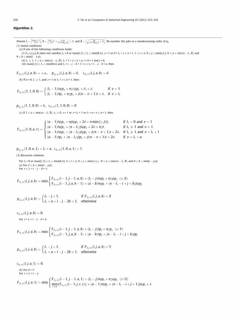
Based on the above analysis, we give a dynamic programmingrecursion as follows:
230 Y. Yin et al. / Computers & Industrial Engineering 63 (2012) 223–234
Algorithm 2.
Denote L ¼ nðbu�cÞbþh
l m, R ¼ nðb�cÞ
bþh þdþbt
ðbþhÞpminw
j kþ 1, and B ¼
ffiffiffiffiffiffiffiffiffiffiffiffiffiffiffiffiffiffiffiffiffiffiffiffiffiffiffi4d
ðbþhÞpminwþ 1qj k
. Re-number the jobs in a nondecreasing order of pj.
(1) Initial conditions(a) If one of the following conditions holds:
(i) (l1,v, i, j,a,b) does not satisfies l1 = 0 or max{L,1} 6 l1 6min{R,n}, v = 1 or 0 < l1 < v 6 n + 1, 1 6 i 6 n, 0 6 j 6min{i, l1}, 0 6 a 6 minfn� l1;Bg and0 6 b 6min{i � j,a},
(ii) l1 P 1, 1 6 a 6minfn� l1;Bg, l1 + 1 < v 6 l1 + a, i = b = 1 and j = 0,(iii) max{L,1} 6 l1 6min{R,n} and l1 + i � j � b + 1 < v 6 l1 + i � j � b + a, then
Fðl1 ;vÞði; j; a; bÞ ¼ þ1; pðl1 ;vÞði; j; a; bÞ ¼ ;; iðl1 ;vÞði; j; a; bÞ ¼ ;:
(b) If a = 0, l1 P 1, and v = 1 or l1 < v 6 n + 1, then
Fðl1 ;vÞð1;1;0;0Þ ¼ðl1 � 1Þhwp1 þ ncðwp1 þ tÞ þ d; if v ¼ 1ðl1 � 1Þhp1 þ ncp1 þ bðn� v þ 1Þt þ d; if v > l1
pðl1 ;vÞð1;1;0;0Þ ¼ l1; iðl1 ;vÞð1;1;0;0Þ ¼ 0
(c) If 1 6 a 6minfn� l1;Bg, l1 P 0, v = 1 or v = l1 + 1 or l1 + a < v 6 n + 1, then
Fðl1 ;vÞð1;0; a;1Þ ¼
ða� 1Þhwp1 þ nbwp1 þ 2dþ n minfc; bgt; if l1 ¼ 0 and v ¼ 1ða� 1Þhwp1 þ ðn� l1Þbwp1 þ 2dþ nct; if l1 P 1 and v ¼ 1ða� 1Þhwp1 þ ðn� l1Þbwp1 þ bðn� v þ 1Þt þ 2d; if l1 P 1 and v ¼ l1 þ 1ða� 1Þhp1 þ ðn� l1Þbp1 þ bðn� v þ 1Þt þ 2d; if v > l1 þ a
8>>><>>>:
pðl1 ;vÞð1;0; a;1Þ ¼ l1 þ a; iðl1 ;vÞð1;0; a;1Þ ¼ 1:
(2) Recursive relations
For l1 = 0 or max{L,1} 6 l1 6min{R,n}, 2 6 i 6 n, 0 6 j 6 minfi; l1g; 0 6 a 6minfn� l1;Bg and 0 6 b 6min{i � j,a}:
(a) For 2 6 b 6min{i � j,a}:For v 6 l1 + i � j � b + 1:
Fðl1 ;vÞði; j; a; bÞ ¼minFðl1 ;vÞði� 1; j� 1; a; bÞ þ ðl1 � jÞhwpi þ ncwpi; ð� XÞFðl1 ;vÞði� 1; j; a; b� 1Þ þ ða� bÞhwpi þ ðn� l1 � iþ jþ bÞbwpi
(
pðl1 ;vÞði; j; a; bÞ ¼l1 � jþ 1; if Fðl1 ;vÞði; j; a; bÞ ¼ Xl1 þ aþ i� j� 2bþ 1; otherwise
iðl1 ;vÞði; j; a; bÞ ¼ 0:
For v > l1 + i � j � b + a:
Fðl1 ;vÞði; j; a; bÞ ¼minFðl1 ;vÞði� 1; j� 1; a; bÞ þ ðl1 � jÞhpi þ ncpi; ð� YÞFðl1 ;vÞði� 1; j; a; b� 1Þ þ ða� bÞhpi þ ðn� l1 � iþ jþ bÞbpi
(
pðl1 ;vÞði; j; a; bÞ ¼l1 � jþ 1; if Fðl1 ;vÞði; j; a; bÞ ¼ Y ;
l1 þ aþ i� j� 2bþ 1; otherwise
iðl1 ;vÞði; j; a;1Þ ¼ 0:
(b) For b = 1:For v 6 l1 + i � j:
Fðl1 ;vÞði; j; a;1Þ ¼minFðl1 ;vÞði� 1; j� 1; a;1Þ þ ðl1 � jÞhwpi þ ncwpi; ð� UÞmincPafFðl1 ;vÞði� 1; j; c; cÞg þ ða� 1Þhwpi þ ðn� l1 � iþ jþ 1Þbwpi þ d
(
pðl1 ;vÞði; j; a;1Þ ¼l1 � jþ 1; if Fðl1 ;vÞði; j; a;1Þ ¼ Ul1 þ aþ i� j� 1 otherwise:
iðl1 ;vÞði; j; a;1Þ ¼0 if Fðl1 ;vÞði; j; a;1Þ ¼ U1 otherwise
For v > l1 + i � j � 1 + a:
Fðl1 ;vÞði; j; a;1Þ ¼minFðl1 ;vÞði� 1; j� 1; a;1Þ þ ðl1 � jÞhpi þ ncpi; ð� VÞmincPafFðl1 ;vÞði� 1; j; c; cÞg þ ða� 1Þhpi þ ðn� l1 � iþ jþ 1Þbpi þ d
(
pðl1 ;vÞði; j; a;1Þ ¼l1 � jþ 1; if Fðl1 ;vÞði; j; a;1Þ ¼ V ;
l1 þ aþ i� j� 1; otherwise:
iðl1 ;vÞði; j; a;1Þ ¼0; if Fðu;vÞði; j; a;1Þ ¼ V ;
1; otherwise
(3) The optimal solution value is F� ¼minfFðl1 ;vÞðn; l1; a; aÞjl1 ¼ 0 or maxfL;1g 6 l1 6 minfR;ng;v ¼ 1 or 0 < l1 < v 6 nþ 1;1 6 a 6 minfn� l1;Bgg.
Y. Yin et al. / Computers & Industrial Engineering 63 (2012) 223–234 231
Let l�1, v� and a⁄ be the corresponding values. The optimal se-quence can be obtained by recursively searching the position func-tions pðl�1 ;v�Þði; j; a; bÞ beginning from pðl�1 ;v�Þðn; l
�1; a
�; a�Þ. By Lemma3.1, the optimal schedule is to process the jobs by the optimal se-quence without any idle except the rate-modifying activity. Theoptimal common due date d is the completion time of the l�1thjob in the optimal schedule if l�1 > 0, and 0 or t otherwise, and itis optimal to perform the rate-modifying activity just before thev⁄th job. The optimal batch delivery date of each job can be deter-mined from the batch indicator functions iðl�1 ;v�Þði; j; a; bÞ.
Theorem 4.3. The problem 1jrm;B; CON;w1 6 wj ¼ w < 1jPn
j¼1ðaEj
þbTj þ hHj þ cdÞ þ dm can be solved in O(n6) time by Algorithm 2.
Proof. Optimality is guaranteed by Lemmas 3.1, 3.2, 3.3, 3.4, 3.5,3.6, 3.7, 3.8, 3.9, 4.1, 4.2, and the principles underlying dynamicprogramming. We now consider the computational complexity ofthe dynamic programming solution algorithm. We have at mostn6 states when b P 2 and at most n5 states when b = 1. Computingeach Fðl1 ;vÞði; j; a; bÞ requires constant time when b P 2, while com-puting each Fðl1 ;vÞði; j; a;1Þ requires O(n) time when b = 1, so com-puting all of them requires O(n6) time. Computing F⁄ requireslinear time. The overall computational complexity of the algorithmis therefore dominated by the former quantity. h
Next we further consider the special case when n(b � c) 62b � h.
Lemma 4.4. For the problem 1jrm;B;CON;w1 6 wj ¼ w <
1jPn
j¼1ðaEj þ bTj þ hHj þ cdÞ þ dm, if n(b � c) 6 2b � h, then pi 6 pj
if Ji is in the early batch B1 and Jj is in the first tardy batch B2.
Proof. If there is no early job, the result is clearly true. In thesequel we assume that there are at least one early job. Becauseof Lemma 3.6, the condition of Lemma 4.4 holds for an optimalschedule if and only if pi 6 pj, where Ji is the first job in B1 and Jj
is the last job in B2. Now suppose that there exists an optimal sche-dule S such that pi > pj, where Ji is the first job in B1 and Jj is the lastjob in B2. Without loss of generality, suppose that the rate-modify-
ing activity is performed just before the first job in B2. The othercases for performing the rate-modifying activity can be similarlyproved. Consider a new schedule S0 constructed by swapping jobsJi and Jj. By Eq. (6), the difference between the objective values ofschedules S0 and S is
D ¼ �ncðpi � pjÞ þ bðn� jB1jÞðpi � pjÞwþ hðjB2j � 1Þðpi � pjÞw6 ð�ncþ bðn� jB1jÞ þ hðjB2j � 1ÞÞðpi � pjÞw¼ ððb� cÞn� ðbjB1j � hðjB2j � 1ÞÞÞðpi � pjÞw:
Since b P h, jB1jP jB2j and n(b � c) 6 2b � h, we have bjB1j � h(jB2j � 1) P 2b � h P (b � c)n, implying that D is nonpositive sincepi > pj. Thus, schedule S0 is at least as good as S. Repeating this mod-ifying argument for all the jobs not sequenced in the specifiedorder yields the result. h
Following Theorem 3.10, Lemmas 4.1, and 4.4, the problem1jrm;B;CON;w1 6 wj ¼ w < 1j
Pnj¼1ðaEj þ bTj þ hHj þ cdÞ þ dm is
solvable in O(n4 logn) time if n(b � c) 6 2b � h by applying Algo-rithm 1 to the jobs in sequence S that is in the SPT order. However,since the optimal job sequence follows the SPT order, we do notneed to re-order the jobs in the required order while applying Step2 of Algorithm 1. Rather, we can re-define Fðl;vÞðj; lÞ as follows:
Fðl1 ;vÞðj; lÞ¼
bðn� jþ1ÞwPl�1
k¼jp½k� if v ¼1 or l1 <v 6 j;
þhwPl�1
k¼jðk� jÞp½l�kþj�1� þdþFðl1 ;vÞðlÞ
bðn� jþ1ÞPl�1
k¼jp½k� if l6 v;
þhPl�1
k¼jðk� jÞp½l�kþj�1� þdþFðl1 ;vÞðlÞ
8>>>>>>>>>>>>>><>>>>>>>>>>>>>>:
which meets the requirement while calculating the holding cost.This allows us to calculate the value of each state in Algorithm 1in a constant time. Based on the above analysis, we have the follow-ing result.
Theorem 4.5. The problem 1jrm;B;CON;w1 6 wj ¼ w < 1jPn
j¼1ðaEj þ bTj þ hHj þ cdÞ þ dm is solvable in O(n4) time if n(b � c)6 2b � h by Algorithm 1 with S that is in the SPT order.
232 Y. Yin et al. / Computers & Industrial Engineering 63 (2012) 223–234
4.2. The case with identical processing times
In this subsection we investigate another special case where thejobs have equal processing times, i.e., pj = p, and show that this spe-cial case, denoted as 1jrm;B;CON; pj ¼ pj
Pnj¼1ðaEj þbTj þ hHj
þcdÞ þ dm, is solvable in O(n5) time. In what follows, suppose thatthe jobs are indexed in a nondecreasing order of wj. If the rate-modifying activity is performed just before the job in position v,then clearly it is optimal to assign the last v � 1 jobs to the firstv � 1 positions, since the processing times of all the jobs beforethe rate-modifying activity are equal. Based on this, we providetwo useful lemmas.
Lemma 4.6. For the problem 1jrm;B;CON; pj ¼ pjPn
j¼1ðaEj þ bTj
þhHj þ cdÞ þ dm, if the rate-modifying activity is performed just beforethe job in position v, then an optimal schedule exists such that the jobs inany two consecutive tardy batches Bk and Bk+1 scheduled after the rate-modifying activity satisfy wi 6wj if Ji is in Bk and Jj is in Bk+1.
Proof. The proof is similar to that of Lemma 4.1. h
Lemma 4.7. For the problem 1jrm;B;CON; pj ¼ pjPn
j¼1ðaEj þ bTj
þhHj þ cdÞ þ dm, if the rate-modifying activity is performed justbefore the job in position v, then an optimal schedule exists such thatjBkjP jBk+1j for any two tardy batches Bk and Bk+1 scheduled before orafter the rate-modifying activity.
Proof. The proof is similar to that of Lemma 4.2. h
Based on the above lemmas, we provide an O(n5) polynomialalgorithm for the problem 1jrm;B;CON; pj ¼ pj
Pnj¼1ðaEj þ bTj
þhHj þ cdÞ þ dm as follows:
Algorithm 3.
Step 1: Re-number the jobs such that w1 6 w2 6 � � � 6 wn.Step 2: For v = 1, apply Algorithm 2 to find the optimal
objective value Fv and the corresponding optimal solution.Step 3: For 1 < v 6 n + 1, we have l1 < v. For this case, schedule
the first n � v + 1 jobs to the last n � v + 1 positions byapplying Algorithm 2, and schedule the last v � 1 jobs tothe first v � 1 positions by applying Algorithm 1. Find theoptimal objective value Fv and the corresponding optimalsolution.
Step 4: The optimal objective value is given bymin{Fvj1 6 l1 6 n + 1}.
Theorem 4.8. Algorithm 3 solves the problem 1jrm;B;CON; pj ¼pjPn
j¼1 ðaEj þbTj þ hHj þ cdÞ þ dm in O(n5) time.
Proof. The correctness of Algorithm 3 follows directly from Lem-mas 4.6 and 4.7. We now consider the computational complexityof the dynamic programming solution algorithm. Step 1 needsO(n logn) time. In Step 2, since v is given, we remove one state var-iable when applying Algorithm 2, so Step 2 requires O(n5) time. InStep 3, for any given v (1 < v 6 n + 1), we have l1 < v, so we removethree state variables and one state variable when applying Algo-rithms 2 and 1 to schedule the first n � v + 1 and the last v � 1 jobs,respectively. Hence Step 3 needs O(n4) time by Theorems 4.3 and4.5. Step 4 needs O(n). Therefore, the overall time complexity ofthe algorithm is O(n5). h
4.3. The case where the jobs and modifying rates are agreeable
In this subsection we investigate the special case, where thejobs and modifying rates are agreeable, i.e., wipi 6 wjpj impliespi 6 pj for all jobs Ji and Jj. This includes the cases where the jobshave equal processing times or where the jobs have equal modify-ing rates. The agreeable condition means that the processing timesof the shorter jobs are even smaller after the rate-modifying activ-ity. We show that this special case of the problem is solvable inO(n4) time if d 6 bwipi + hwjpj for all jobs Ji and Jj by a dynamic pro-gramming algorithm. We begin with providing two useful lemmas.
Lemma 4.9. For the problem 1jrm;B;CONjPn
j¼1ðaEj þbTj þhHj
þcdÞ þ dm, if d 6 bwipi + hwjpj for all jobs Ji and Jj, then for all thetardy jobs, the optimal policy is to ship each one as it finishes.
Proof. Suppose that there exists an optimal schedule S in which atardy batch Bk ¼ fJ½lk�1þ1�; � � � ; J½lk �g has more than one job. Further-more, suppose that the rate-modifying activity is performed beforeBk. The case where the rate-modifying activity is performed after Bk
can be similarly proved. Consider a new schedule S0 constructed bysplitting bath Bk into two batches fJ½lk �g and fJ½lk�1þ1�; . . . ; J½lk�1�g. ByEq. (6), the difference between the objective values of schedulesS0 and S is
D ¼ �bðPkðSÞ � w½lk �p½lk �Þ � hðjBkj � 1Þw½lk �p½lk � þ d
6 �bwjpj � hw½lk �p½lk � þ d;
which is negative by assumption, where Jj is a job Bk. Thus, we canreduce the total cost by removing a job from a multi-job batch anddelivering it separately, as required. h
Lemma 4.10. For the problem 1jrm;B;CONjPn
j¼1ðaEj þ bTj
þhHj þ cdÞ þ dm, if d 6 bwipi + hwjpj for all jobs Ji and Jj, then thetardy jobs scheduled before the rate-modifying activity is sequencedin nondecreasing order of pj and the tardy jobs scheduled after therate-modifying activity are sequenced in nondecreasing order of wjpj.
Proof. It is straightforward by the job interchange argument. h
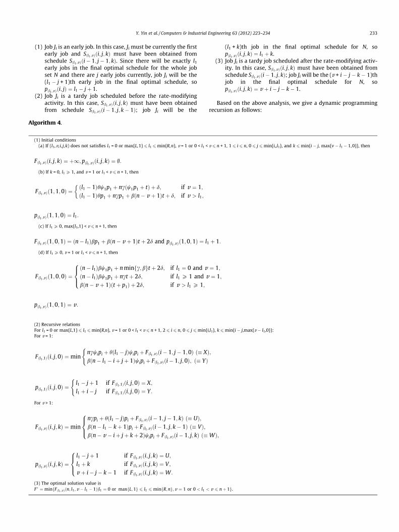
In the remaining part of this section, suppose that the jobs areindexed in a nondecreasing order of wjpj. We next provide a recur-sion relation that can be exploited to design a polynomial dynamicprogramming algorithm for the problem 1jrm;B;CONj
Pnj¼1
ðaEj þ bTj þ hHj þ cdÞ þ dm where the jobs and modifying ratesare agreeable and d 6 bwipi + hwjpj for all jobs Ji and Jj. We beginwith introducing some notation that will be used later:ði; j; kÞðl1 ;vÞ: a state representing the situation, where the jobs
{1, . . . , i} have been scheduled, provided that in the final optimalschedule for the whole job set N, there are exactly l1 early jobsand the rate-modifying activity is scheduled just before the vthjob, and that in the current partial schedule for the jobs {1, . . . , i},there are j (j 6min{i, l1}) early jobs and there are k (k 6min{i � j,max{v � l1 � 1,0}}) tardy jobs scheduled before the rate-modifyingactivity.
Fðl1 ;vÞði; j; kÞ: the optimal solution value of any schedule in stateði; jÞðl1 ;vÞ.
Sðl1 ;vÞði; j; kÞ: any schedule in state ði; jÞðl1 ;v ;kÞ with the solution va-lue Fðl1 ;vÞði; j; kÞ.
pðl1 ;vÞði; j; kÞ: the position number of job Ji in the final optimalschedule for the whole job set N if the jobs {1, . . . , i} are scheduledcorresponding to Fðl1 ;vÞði; j; kÞ. This function is used to keep track ofthe positions of the jobs in the optimal schedule.
By definition, we set Fðl1 ;vÞði; j; kÞ ¼ þ1 if no such schedule ex-ists. Then the schedule Sðl1 ;vÞði; j; kÞ must have been constructedby taking one of the following three decisions in a previous state.
Y. Yin et al. / Computers & Industrial Engineering 63 (2012) 223–234 233
(1) Job Ji is an early job. In this case, Ji must be currently the firstearly job and Sðl1 ;vÞði; j; kÞ must have been obtained fromschedule Sðl1 ;vÞði� 1; j� 1; kÞ. Since there will be exactly l1early jobs in the final optimal schedule for the whole jobset N and there are j early jobs currently, job Ji will be the(l1 � j + 1)th early job in the final optimal schedule, sopðl1 ;vÞði; jÞ ¼ l1 � jþ 1.
(2) Job Ji is a tardy job scheduled before the rate-modifyingactivity. In this case, Sðl1 ;vÞði; j; kÞ must have been obtainedfrom schedule Sðl1 ;vÞði� 1; j; k� 1Þ; job Ji will be the
Algorithm 4.
(1) Initial conditions(a) If (l1,v, i, j,k) does not satisfies l1 = 0 or max{L,1} 6 l1 6min{R,n}, v = 1 or 0 < l1 <
Fðl1 ;vÞði; j; kÞ ¼ þ1;pðl1 ;vÞði; j; kÞ ¼ ;:
(b) If k = 0, l1 P 1, and v = 1 or l1 < v 6 n + 1, then
Fðl1 ;vÞð1;1;0Þ ¼ðl1 � 1Þhw1p1 þ ncðw1p1 þ tÞ þ d; if v ¼ 1;ðl1 � 1Þhp1 þ ncp1 þ bðn� v þ 1Þt þ d; if v > l1;
pðl1 ;vÞð1;1;0Þ ¼ l1:
(c) If l1 P 0, max{l1,1} < v 6 n + 1, then
Fðl1 ;vÞð1;0;1Þ ¼ ðn� l1Þbp1 þ bðn� v þ 1Þt þ 2d and pðl1 ;vÞð1;0;1Þ ¼ l1
(d) If l1 P 0, v = 1 or l1 < v 6 n + 1, then
Fðl1 ;vÞð1;0;0Þ ¼ðn� l1Þbw1p1 þ n minfc;bgt þ 2d; if l1 ¼ 0 and vðn� l1Þbw1p1 þ nct þ 2d; if l1 P 1 and vbðn� v þ 1Þðt þ p1Þ þ 2d; if v > l1 P 1;
8><>:
pðl1 ;vÞð1;0;1Þ ¼ v:
(2) Recursive relationsFor l1 = 0 or max{L,1} 6 l1 6min{R,n}, v = 1 or 0 < l1 < v 6 n + 1, 2 6 i 6 n, 0 6 j 6min{For v = 1:
Fðl1 ;1Þði; j;0Þ ¼ minncwipi þ hðl1 � jÞwipi þ Fðl1 ;vÞði� 1; j� 1;0Þ ð� XÞbðn� l1 � iþ jþ 1Þwipi þ Fðl1 ;vÞði� 1; j;0Þ; ð� YÞ
(
pðl1 ;1Þði; j;0Þ ¼l1 � jþ 1 if Fðl1 ;1Þði; j;0Þ ¼ X;
l1 þ i� j if Fðl1 ;1Þði; j;0Þ ¼ Y :
(
For v > 1:
Fðl1 ;vÞði; j; kÞ ¼minncpi þ hðl1 � jÞpi þ Fðl1 ;vÞði� 1; j� 1; kÞ ð� UÞ;bðn� l1 � kþ 1Þpi þ Fðl1 ;vÞði� 1; j; k� 1Þ ð� VÞ;bðn� v � iþ jþ kþ 2Þwipi þ Fðl1 ;vÞði� 1; j; kÞ ð�
8><>:
pðl1 ;vÞði; j; kÞ ¼l1 � jþ 1 if Fðl1 ;vÞði; j; kÞ ¼ U;
l1 þ k if Fðl1 ;vÞði; j; kÞ ¼ V ;
v þ i� j� k� 1 if Fðl1 ;vÞði; j; kÞ ¼W:
8><>:
(3) The optimal solution value isF� ¼minfFðl1 ;vÞðn; l1; v � l1 � 1Þjl1 ¼ 0 or maxfL;1g 6 l1 6minfR;ng; v ¼ 1 or 0 < l1 <
(l1 + k)th job in the final optimal schedule for N, sopðl1 ;vÞði; j; kÞ ¼ l1 þ k.
(3) Job Ji is a tardy job scheduled after the rate-modifying activ-ity. In this case, Sðl1 ;vÞði; j; kÞ must have been obtained fromschedule Sðl1 ;vÞði� 1; j; kÞ; job Ji will be the (v + i � j � k � 1)thjob in the final optimal schedule for N, sopðl1 ;vÞði; j; kÞ ¼ v þ i� j� k� 1.
Based on the above analysis, we give a dynamic programmingrecursion as follows:
v 6 n + 1, 1 6 i 6 n, 0 6 j 6min{i,,l1}, and k 6min{i � j, max{v � l1 � 1,0}}, then
þ 1:
¼ 1;¼ 1;
i,l1}, k 6min{i � j,max{v � l1,0}}:
;
WÞ;
v 6 nþ 1g.
234 Y. Yin et al. / Computers & Industrial Engineering 63 (2012) 223–234
Let l�1 and v⁄ be the corresponding values. The optimal sequencecan be obtained by recursively searching the position functionp l�1 ;v�ð Þði; j; kÞ beginning with p l�1 ;v�ð Þ n; l�1;v� � l�1 � 1
�. By Lemma
3.1, the optimal schedule is to process the jobs in the optimal se-quence without any idle time except the rate-modifying activity.The optimal common due date d is the completion time of thel�1th job in the optimal schedule if l�1 > 0, and 0 or t otherwise,and it is optimal to perform the rate-modifying activity just beforethe v⁄th job.
Theorem 4.11. The problem 1jrm;B;CONjPn
j¼1ðaEj þ bTj þ hHj
þcdÞ þ dm can be solved in O(n5) time by Algorithm 3 if the jobsand modifying rates are Agreeable, and d 6 bwipi + hwjpj for all jobs Ji
and Jj.
Proof. The proof is similar to that of Theorem 4.3. h
5. Conclusions
In this paper we consider single-machine scheduling withsimultaneous consideration of batch delivery cost, common duedate assignment, and a rate-modifying activity. The objective isto minimize the sum of earliness, tardiness, holding, due date,and delivery cost. We investigate the structural properties of theoptimal schedule of the problem and obtain the following results:
(i) the problem can be solved in O(n6) time if w1 6 wj = w;(ii) the problem can be solved in O(n4) time if w1 6 wj = w and
n(b � c) 6 2b � h;(iii) the problem can be solved in O(n5) time if pj = p;(iv) the problem can be solved in O(n5) time if the jobs and mod-
ifying rates are agreeable and d 6 bwipi + hwjpj for all jobs Ji
and Jj.
The computational complexity of the problem 1jrm;B;CONj
Pnj¼1ðaEj þ bTj þ hHj þ cdÞ þ dm is still open, which future re-
search should study.
Acknowledgements
This paper was supported in part by the Natural Science Foun-dation for Young Scholars of Jiangxi, China (2010GQS0003); in partby the Science Foundation of Education Committee for YoungScholars of Jiangxi, China (GJJ11143); and in part by the NSC underGrant No. NSC 99-2221-E-035-057-MY3.
References
Adamopoulos, G. I., & Pappis, C. P. (1995). The CON due-date determination methodwith processing time-dependent lateness penalties. International Journal ofProduction Economics, 40, 29–36.
Birman, M., & Mosheiov, G. (2004). A note on a due-date assignment on a two-machine flow-shop. Computers and Operations Research, 31, 473–480.
Biskup, D., & Jahnke, H. (2001). Common due date assignment for scheduling on asingle machine with jointly reducible processing times. International Journal ofProduction Economics, 69, 317–322.
Chen, Z. L. (1996). Scheduling and common due date assignment with earliness-tardiness penalties and batch delivery costs. European Journal of OperationalResearch, 93, 49–60.
Cheng, T. C. E. (1984). Optimal due-date determination and sequencing of n jobs ona single machine. Journal of the Operational Research Society, 35, 433–437.
Cheng, T. C. E. (1987). An algorithm for the CON due-date determination andsequencing problem. Computers and Operations Research, 14, 537–542.
Cheng, T. C. E. (1989). A heuristic for common due-date assignment and jobscheduling on parallel machines. Journal of the Operational Research Society, 40,1129–1135.
Cheng, T. C. E., Chen, Z.-L., & Shakhlevich, N. V. (2002). Common due dateassignment and scheduling with ready times. Computers and OperationsResearch, 29, 1957–1967.
Cheng, T. C. E., & Gordon, V. S. (1994). Batch delivery scheduling on a singlemachine. Journal of the Operational Research Society, 45, 1211–1215.
Cheng, T. C. E., & Gupta, M. C. (1989). Survey of scheduling involving due datedetermination decisions. European Journal of Operational Research, 38,156–166.
Cheng, T. C. E., & Kahlbacher, H. G. (1993). Scheduling with delivery and earlinesspenalty. Asia-Pacific Journal of Operational Research, 10, 145–152.
Cheng, T. C. E., Kang, L. Y., & Ng, C. T. (2004). Due-date assignment and singlemachine scheduling with deteriorating jobs. Journal of the Operational ResearchSociety, 55, 198–203.
Cheng, T. C. E., Kang, L. Y., & Ng, C. T. (2007). Due-date assignment and parallel-machine scheduling with deteriorating jobs. Journal of the Operational ResearchSociety, 58, 1103–1108.
De, P., Ghosh, J. B., & Wells, C. E. (1991). Optimal delivery time quotation and ordersequencing. Decision Sciences, 22, 379–390.
Gordon, V., Strusevich, V., & Dolgui, A. (2010). Scheduling with due date assignmentunder special conditions on job processing. Journal of Scheduling, doi:10.1007/s10951-011-0240-2.
Gordon, V., Proth, J. M., & Chu, C. B. (2002). A survey of the state-of-the-art ofcommon due date assignment and scheduling research. European Journal ofOperational Research, 139, 1–25.
Gordon, V. S., & Strusevich, V. A. (2009). Single machine scheduling and due dateassignment with positional dependent processing times. European Journal ofOperational Research, 198, 57–62.
Gordon, V. S., & Tarasevich, A. A. (2009). A note: Common due date assignment for asingle machine scheduling with the rate-modifying activity. Computers andOperations Research, 36, 325–328.
Hermann, J. W., & Lee, C. Y. (1993). On scheduling to minimize earliness-tardinessand batch delivery costs with a common due date. European Journal ofOperational Research, 70, 272–288.
Hsu, C.-J., Yang, S.-J., & Yang, D.-L. (2011). Two due date assignment problems withposition-dependent processing time on a single-machine. Computers &Industrial Engineering, 60, 796–800.
Kahlbacher, H. G., & Cheng, T. C. E. (1993). Parallel machine scheduling to minimizecosts for earliness and number of tardy jobs. Discrete Applied Mathematics, 47,139–164.
Lauff, V., & Werner, F. (2004). Scheduling with common due date, earliness andtardiness penalties for multimachine problems: A survey. Mathematical andComputer Modelling, 40, 637–655.
Lee, C.-Y., & Leon, V. J. (2001). Machine scheduling with a rate-modifying activity.European Journal of Operational Research, 128, 119–128.
Li, S., Ng, C. T., & Yuan, J. J. (2011). Scheduling deteriorating jobs with CON/SLK duedate assignment on a single machine. International Journal of ProductionEconomics, 131, 747–751.
Lodree, E. J., & Geiger, C. D. (2010). A note on the optimal sequence position for arate-modifying activity under simple linear deterioration. European Journal ofOperational Research, 201, 644–648.
Min, L., & Cheng, W. (2006). Genetic algorithms for the optimal common due dateassignment and the optimal scheduling policy in parallel machine earliness/tardiness scheduling problems. Robotics and Computer-Integrated Manufacturing,22, 279–287.
Mosheiov, G. (2001). A common due-date assignment problem on parallel identicalmachines. Computers and Operations Research, 28(8), 719–732.
Mosheiov, G., & Oron, D. (2006). Due-date assignment and maintenanceactivity scheduling problem. Mathematical and Computer Modelling, 44,1053–1057.
Mosheiov, G., & Sidney, J. B. (2004). New results on sequencing with ratemodification. INFOR, 41, 155–163.
Mosheiov, G., & Yovel, U. (2006). Minimizing weighted earliness tardiness and due-date cost with unit processing time jobs. European Journal of OperationalResearch, 172, 528–544.
Ng, C. T., Cheng, T. C. E., Kovalyov, M. Y., & Lam, S. S. (2003). Single machinescheduling with a variable common due date and resource-dependentprocessing times. Computers and Operations Research, 30, 1173–1185.
Panwalkar, S. S., Smith, M. L., & Seidmann, A. (1982). Common due date assignmentto minimize total penalty for the one machine scheduling problem. OperationsResearch, 30, 391–399.
Shabtay, D. (2010). Scheduling and due date assignment to minimize earliness,tardiness, holding, due date assignment and batch delivery costs. InternationalJournal of Production Economics, 123, 235–242.
Shabtay, D., & Steiner, G. (2006). Two due date assignment problems in scheduling asingle machine. Operations Research Letters, 34, 683–691.
Wang, X. Y., & Wang, M. Z. (2010). Single machine common flow allowancescheduling with a rate-modifying activity. Computers & Industrial Engineering,59, 898–902.
Yin, Y., Cheng, T. C. E., Hsu, C.-J., & Wu, C.-C. (submitted for publication). Single-machine batch delivery scheduling with an assignable common due window.Omega.
Yin, Y., Cheng, T. C. E., Wu, C.-C., & Cheng, S.-R. (submitted for publication). Commondue date assignment and single-machine batch delivery scheduling with a rate-modifying activity. Discrete Applied Mathematics.
Zhao, C. L., Tang, H. Y., & Cheng, C. D. (2009). Two-parallel machines scheduling withrate-modifying activities to minimize total completion time. European Journal ofOperational Research, 198, 354–357.