Embed Size (px)
Citation preview
COMMUNICATION IN NETWORKS
FOR COORDINATING BEHAVIOR
A DISSERTATION
SUBMITTED TO THE DEPARTMENT OF ELECTRICAL
ENGINEERING
AND THE COMMITTEE ON GRADUATE STUDIES
OF STANFORD UNIVERSITY
IN PARTIAL FULFILLMENT OF THE REQUIREMENTS
FOR THE DEGREE OF
DOCTOR OF PHILOSOPHY
Paul W. Cuff
July 2009

c© Copyright by Paul W. Cuff 2009
All Rights Reserved
ii

I certify that I have read this dissertation and that, in my opinion, it
is fully adequate in scope and quality as a dissertation for the degree
of Doctor of Philosophy.
(Thomas M. Cover) Principal Adviser
I certify that I have read this dissertation and that, in my opinion, it
is fully adequate in scope and quality as a dissertation for the degree
of Doctor of Philosophy.
(Tsachy Weissman)
I certify that I have read this dissertation and that, in my opinion, it
is fully adequate in scope and quality as a dissertation for the degree
of Doctor of Philosophy.
(Abbas El Gamal)
Approved for the University Committee on Graduate Studies.
iii
Preface
The theory of information, as charted by Claude Shannon, has influenced many fields
and introduced a new way of thinking about information. Beyond the immediate
applications to digital communication, the ideas introduced by information theory
have found their way into the study of biology and DNA, computation and complexity,
and machine learning. Indeed, the field provides a concrete way of dealing with the
otherwise nebulous substance of information. Although many of the basic questions
have been answered, even by Shannon himself, many fundamental questions dealing
with multiple users and multiple sources of information have remained unanswered
for decades. We are still lacking in our understanding of how to best structure and
correlate codebooks for communicating in network settings. Answers to the building
blocks of network information theory provide insight into how information can be
reinforced in a complex setting, ultimately giving us principles for better technology
and greater understanding.
Beyond the intriguing array of classical open problems related to communicating
in networks, the field itself is open to broader interpretation. By considering new
purposes for communication, besides transporting information from one location to
another, we find many new problems of interest.
In this work, we develop elements of a theory of coordination in networks. With
rate-limited communication between the nodes of a network, we ask for the set of all
possible joint distributions p(x1, ..., xm) of actions at the nodes. Several networks are
solved, including arbitrarily large cascade networks. Distributed coordination can be
the solution to many problems such as distributed games, distributed control, and
establishing bounds on the physical influence of one part of a system on another.
iv

Acknowledgement
Larisa and I made a decision in 2004 to move out to California, live in cramped
graduate student housing, raise a small family while we’re at it, and enjoy a Stanford
education. First and foremost I thank her for giving me the opportunity.
It was clear from the beginning of graduate school that I would enjoy going deeper
in familiar areas of science, math, and engineering. But it came as a surprise that
my depth would ultimately be developed in a field completely unknown to me at the
start. The door to an entirely new way of thinking was hiding behind a few well-
taught lectures and fascinating conversations. If anyone wonders how I lost focus
during my time at Stanford, I have Tom Cover to blame, for leaking the best-kept
secrets of applied math and engineering. He taught me not only information theory
but to continually look for the big picture and let curiosity guide. He made my grad
school experience.
A number of other mentors will have a lasting influence on me, including Tsachy
Weissman, Abbas El Gamal, Balaji Prabhakar, and Bernard Widrow. We’ve had fun
adventures and collaborations together.
For all the times I needed a friend, colleague, baby-sitter, or brain, Haim Permuter
was there from day one. We started graduate school together, and not long after I
introduced him to information theory he was trying to get me to commit as well.
Each member of Tom Cover’s and Tsachy Weissman’s research groups became a
close friend. Young-Han Kim in particular served not only as a friend but also as an
adviser for career and research decisions.
v
Contents
Preface iv
Acknowledgement v
1 Coordination of Actions 1
2 Empirical Coordination 6
2.1 Introduction . . . . . . . . . . . . . . . . . . . . . . . . . . . . . . . . 6
2.1.1 Preliminary observations . . . . . . . . . . . . . . . . . . . . . 9
2.1.2 Generalize . . . . . . . . . . . . . . . . . . . . . . . . . . . . . 11
2.2 Network results . . . . . . . . . . . . . . . . . . . . . . . . . . . . . . 12
2.2.1 Two nodes . . . . . . . . . . . . . . . . . . . . . . . . . . . . . 12
2.2.2 Isolated node . . . . . . . . . . . . . . . . . . . . . . . . . . . 14
2.2.3 Cascade . . . . . . . . . . . . . . . . . . . . . . . . . . . . . . 17
2.2.4 Degraded source . . . . . . . . . . . . . . . . . . . . . . . . . 19
2.2.5 Broadcast . . . . . . . . . . . . . . . . . . . . . . . . . . . . . 21
2.3 Rate-distortion theory . . . . . . . . . . . . . . . . . . . . . . . . . . 34
2.4 Proofs . . . . . . . . . . . . . . . . . . . . . . . . . . . . . . . . . . . 37
2.4.1 Achievability . . . . . . . . . . . . . . . . . . . . . . . . . . . 37
2.4.2 Converse . . . . . . . . . . . . . . . . . . . . . . . . . . . . . . 48
2.4.3 Rate-distortion . . . . . . . . . . . . . . . . . . . . . . . . . . 56
3 Strong Coordination 59
3.1 Introduction . . . . . . . . . . . . . . . . . . . . . . . . . . . . . . . . 59
vi
3.1.1 Problem specifics . . . . . . . . . . . . . . . . . . . . . . . . . 60
3.1.2 Preliminary observations . . . . . . . . . . . . . . . . . . . . . 61
3.2 No communication . . . . . . . . . . . . . . . . . . . . . . . . . . . . 62
3.3 Two nodes . . . . . . . . . . . . . . . . . . . . . . . . . . . . . . . . . 65
3.3.1 Insights . . . . . . . . . . . . . . . . . . . . . . . . . . . . . . 69
3.4 Game theory . . . . . . . . . . . . . . . . . . . . . . . . . . . . . . . 71
3.5 Proofs . . . . . . . . . . . . . . . . . . . . . . . . . . . . . . . . . . . 74
3.5.1 Achievability . . . . . . . . . . . . . . . . . . . . . . . . . . . 76
3.5.2 Converse . . . . . . . . . . . . . . . . . . . . . . . . . . . . . . 85
4 Extension 97
Bibliography 101
vii
Chapter 1
Coordination of Actions
Communication is required to establish cooperative behavior. In a network of nodes
where relevant information is known at only some nodes in the network, finding the
minimum communication requirements to coordinate actions can be posed as a net-
work source coding problem. This breaks somewhat from traditional source coding.
Rather than focusing on sending data from one point to another with a fidelity con-
straint, we can consider the communication needed to establish coordination summa-
rized by a joint probability distribution of behavior among all nodes in the network.
A large variety of research addresses the challenge of collecting or moving infor-
mation in networks. Network coding [1] seeks to efficiently move independent flows of
information over shared communication links. On the other hand, distributed average
consensus [2] involves collecting related information. Sensors in a network collectively
compute the average of their measurements in a distributed fashion. The network
topology and dynamics determine how many rounds of communication among neigh-
bors are needed to converge to the average and how good the estimate will be at each
node [3]. Similarly, in the gossiping Dons problem [4], each node starts with a unique
piece of gossip, and one wishes to know how many exchanges of gossip are required to
make everything known to everyone. Computing functions in a network is considered
in [5], [6], and [7].
Our work has several distinctions from the network communication examples men-
tioned. First, we keep the purpose for communication very general, which means
1
CHAPTER 1. COORDINATION OF ACTIONS 2
sometimes we get away with saying very little about the information in the network
while still achieving the desired coordination. We are concerned with the joint distri-
bution of actions taken at the various nodes in the network, and the “information”
that enters the network is nothing more than actions that are selected randomly by
nature and assigned to certain nodes. Secondly, we consider quantization and rates of
communication in the network, as opposed to only counting the number of exchanges.
We find that we can gain efficiency by using vector quantization specifically tailored
to the network topology.
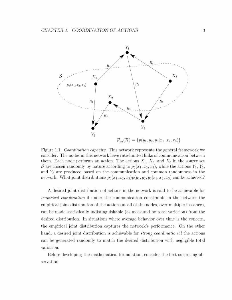
Figure 1.1 shows an example of a network with rate-limited communication links.
In general, each node in the network performs an action where some of these actions
are selected randomly by nature. In this network, the source set S indicates which
actions are chosen by nature: Actions X1, X2, and X3 are assigned randomly ac-
cording to the joint distribution p0(x1, x2, x3). Then, using the communication and
common randomness that is available to all nodes, the actions Y1, Y2, and Y3 outside
of S are produced. We ask, which conditional distributions p(y1, y2, y3|x1, x2, x3) are
compatible with the network constraints.
A variety of applications are encompassed in this framework. This could be used
to model sensors in a sensor network, sharing information in the standard sense, while
also cooperating in their transmission of data. Similarly, a wireless ad hoc network
can improve performance by cooperating among nodes to allow beam-forming and
interference alignment. On the other hand, some settings do not involve moving
information in the usual sense. The nodes in the network might comprise a distributed
control system, where the behavior at each node must be related to the behavior at
other nodes and the information coming into the system. Also, with computing
technology continuing to move in the direction of parallel processing, even across
large networks, a network of computers must coherently perform computations while
distributing the work load across the participating machines. Alternatively, the nodes
might each be agents taking actions in a multiplayer game.
Network communication can be revisited from the viewpoint of coordinated ac-
tions. Rate distortion theory becomes a special case. More generally, we ask how we
can build dependence among the nodes. What is it good for? How do we use it?
CHAPTER 1. COORDINATION OF ACTIONS 3
X1
X2
X3
Y1
Y2
Y3
R1
R2
R3
R4
R5
R6
R7
p0(x1, x2, x3)
S
Pp0(R) = p(y1, y2, y3|x1, x2, x3)
Figure 1.1: Coordination capacity. This network represents the general framework weconsider. The nodes in this network have rate-limited links of communication betweenthem. Each node performs an action. The actions X1, X2, and X3 in the source setS are chosen randomly by nature according to p0(x1, x2, x3), while the actions Y1, Y2,and Y3 are produced based on the communication and common randomness in thenetwork. What joint distributions p0(x1, x2, x3)p(y1, y2, y3|x1, x2, x3) can be achieved?
A desired joint distribution of actions in the network is said to be achievable for
empirical coordination if under the communication constraints in the network the
empirical joint distribution of the actions at all of the nodes, over multiple instances,
can be made statistically indistinguishable (as measured by total variation) from the
desired distribution. In situations where average behavior over time is the concern,
the empirical joint distribution captures the network’s performance. On the other
hand, a desired joint distribution is achievable for strong coordination if the actions
can be generated randomly to match the desired distribution with negligible total
variation.
Before developing the mathematical formulation, consider the first surprising ob-
servation.
CHAPTER 1. COORDINATION OF ACTIONS 4
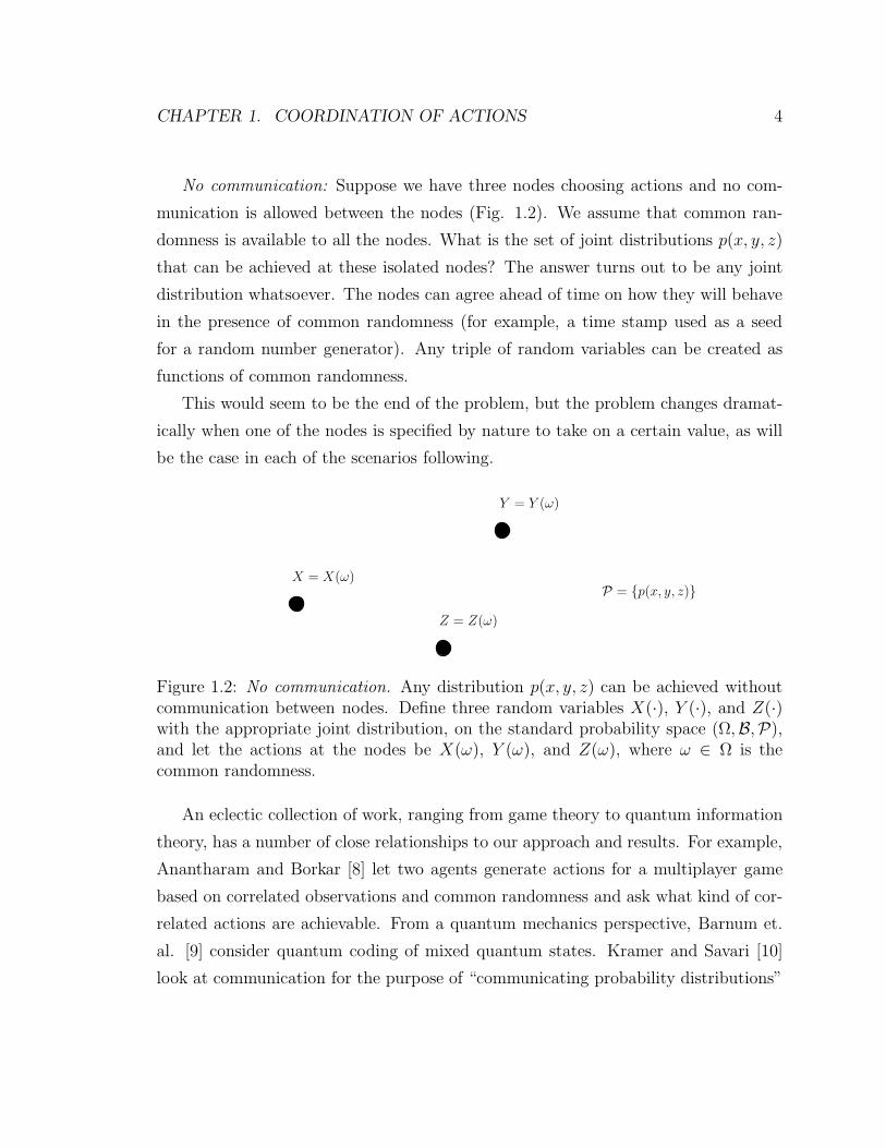
No communication: Suppose we have three nodes choosing actions and no com-
munication is allowed between the nodes (Fig. 1.2). We assume that common ran-
domness is available to all the nodes. What is the set of joint distributions p(x, y, z)
that can be achieved at these isolated nodes? The answer turns out to be any joint
distribution whatsoever. The nodes can agree ahead of time on how they will behave
in the presence of common randomness (for example, a time stamp used as a seed
for a random number generator). Any triple of random variables can be created as
functions of common randomness.
This would seem to be the end of the problem, but the problem changes dramat-
ically when one of the nodes is specified by nature to take on a certain value, as will
be the case in each of the scenarios following.
X = X(ω)
Y = Y (ω)
Z = Z(ω)
P = p(x, y, z)
Figure 1.2: No communication. Any distribution p(x, y, z) can be achieved withoutcommunication between nodes. Define three random variables X(·), Y (·), and Z(·)with the appropriate joint distribution, on the standard probability space (Ω,B,P),and let the actions at the nodes be X(ω), Y (ω), and Z(ω), where ω ∈ Ω is thecommon randomness.
An eclectic collection of work, ranging from game theory to quantum information
theory, has a number of close relationships to our approach and results. For example,
Anantharam and Borkar [8] let two agents generate actions for a multiplayer game
based on correlated observations and common randomness and ask what kind of cor-
related actions are achievable. From a quantum mechanics perspective, Barnum et.
al. [9] consider quantum coding of mixed quantum states. Kramer and Savari [10]
look at communication for the purpose of “communicating probability distributions”
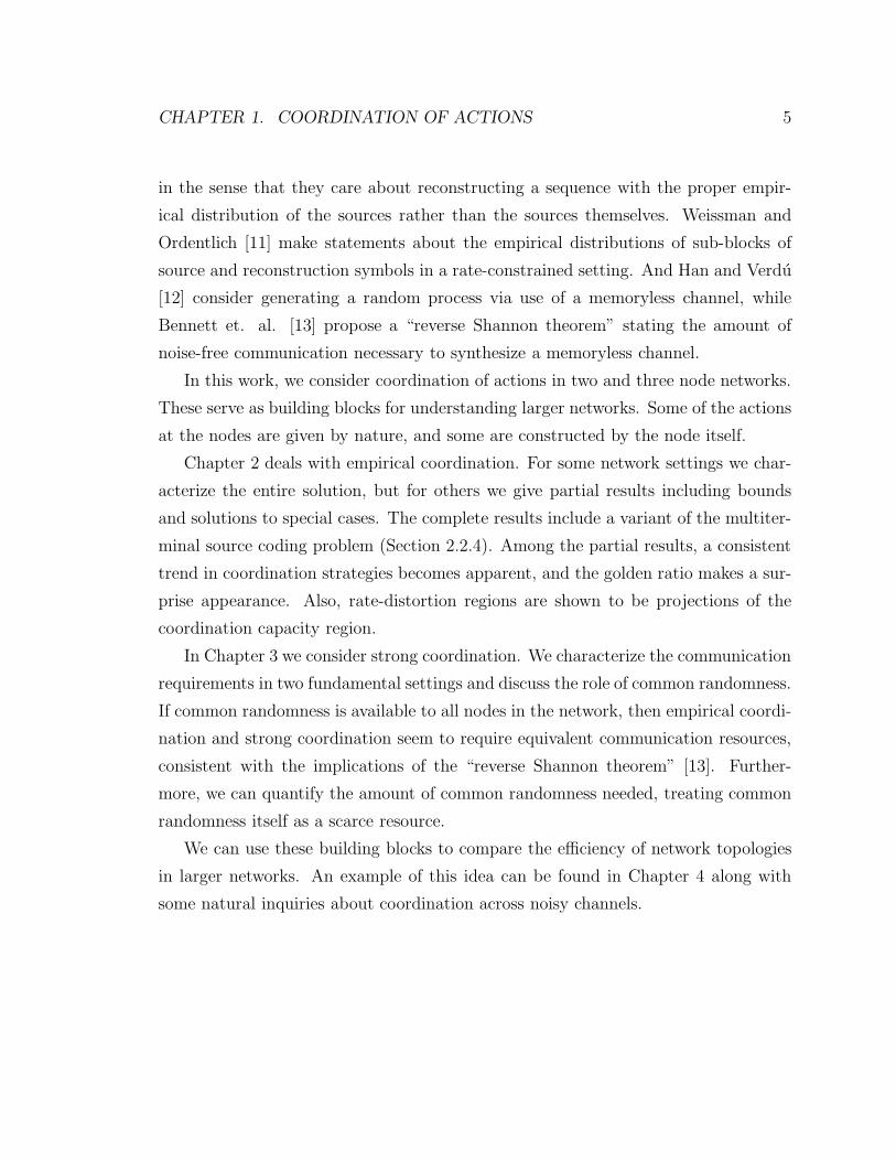
CHAPTER 1. COORDINATION OF ACTIONS 5
in the sense that they care about reconstructing a sequence with the proper empir-
ical distribution of the sources rather than the sources themselves. Weissman and
Ordentlich [11] make statements about the empirical distributions of sub-blocks of
source and reconstruction symbols in a rate-constrained setting. And Han and Verdu
[12] consider generating a random process via use of a memoryless channel, while
Bennett et. al. [13] propose a “reverse Shannon theorem” stating the amount of
noise-free communication necessary to synthesize a memoryless channel.
In this work, we consider coordination of actions in two and three node networks.
These serve as building blocks for understanding larger networks. Some of the actions
at the nodes are given by nature, and some are constructed by the node itself.
Chapter 2 deals with empirical coordination. For some network settings we char-
acterize the entire solution, but for others we give partial results including bounds
and solutions to special cases. The complete results include a variant of the multiter-
minal source coding problem (Section 2.2.4). Among the partial results, a consistent
trend in coordination strategies becomes apparent, and the golden ratio makes a sur-
prise appearance. Also, rate-distortion regions are shown to be projections of the
coordination capacity region.
In Chapter 3 we consider strong coordination. We characterize the communication
requirements in two fundamental settings and discuss the role of common randomness.
If common randomness is available to all nodes in the network, then empirical coordi-
nation and strong coordination seem to require equivalent communication resources,
consistent with the implications of the “reverse Shannon theorem” [13]. Further-
more, we can quantify the amount of common randomness needed, treating common
randomness itself as a scarce resource.
We can use these building blocks to compare the efficiency of network topologies
in larger networks. An example of this idea can be found in Chapter 4 along with
some natural inquiries about coordination across noisy channels.
Chapter 2
Empirical Coordination
2.1 Introduction
In this chapter we address questions of this nature: If three different tasks are to
be performed in a shared effort between three people, but one of them is randomly
assigned his responsibility, how much must he tell the others about his assignment?
We consider coordination in a variety of two and three node networks. The basic
meaning of empirical coordination according to a desired distribution is the same for
each network—we use the network communication to construct a sequence of actions
that have an empirical joint distribution closely matching the desired distribution.
What’s different from one problem to the next is the set of nodes whose actions
are selected randomly by nature and the communication limitations imposed by the
network topology.
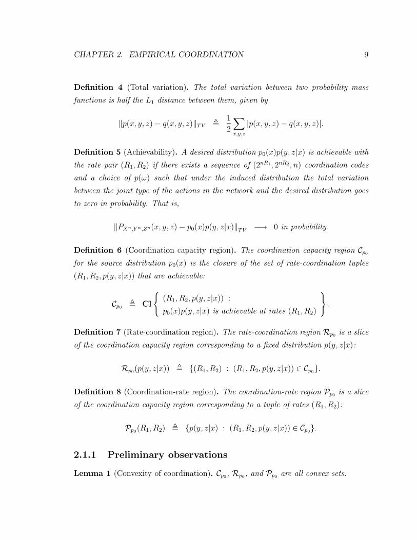
Here we define the problem in the context of the cascade network of Section 2.2.3
shown in Figure 2.1. These definitions have obvious generalizations to other networks.
In the cascade network of Figure 2.1, node X has a sequence of actions X1, X2, ...
specified randomly by nature. Note that a node is allowed to see all of its actions
before it summarizes them for the next node. Communication is used to give Node Y
and Node Z enough information to choose sequences of actions that are empirically
correlated with X1, X2, ... according to a desired joint distribution p0(x)p(y, z|x). The
communication travels in a cascade, first from Node X to Node Y at rate R1 bits per
6
CHAPTER 2. EMPIRICAL COORDINATION 7
Node X
i(Xn, ω)
Node Y
yn(I, ω)j(I, ω)
Node Z
zn(J, ω)Xn
I ∈ [2nR1 ] J ∈ [2nR2 ]Y n Zn
∼∏ni=1 p0(xi)
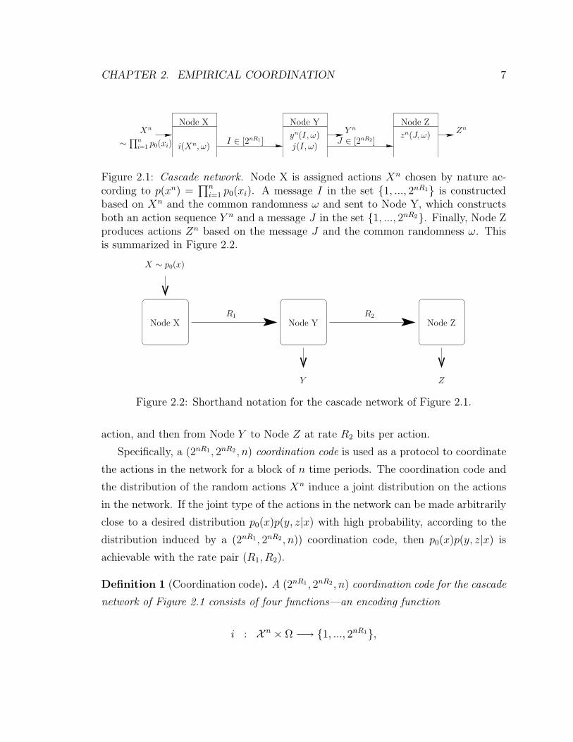
Figure 2.1: Cascade network. Node X is assigned actions Xn chosen by nature ac-cording to p(xn) =
∏ni=1 p0(xi). A message I in the set 1, ..., 2nR1 is constructed
based on Xn and the common randomness ω and sent to Node Y, which constructsboth an action sequence Y n and a message J in the set 1, ..., 2nR2. Finally, Node Zproduces actions Zn based on the message J and the common randomness ω. Thisis summarized in Figure 2.2.
X ∼ p0(x)
Y Z
R1 R2
Node X Node Y Node Z
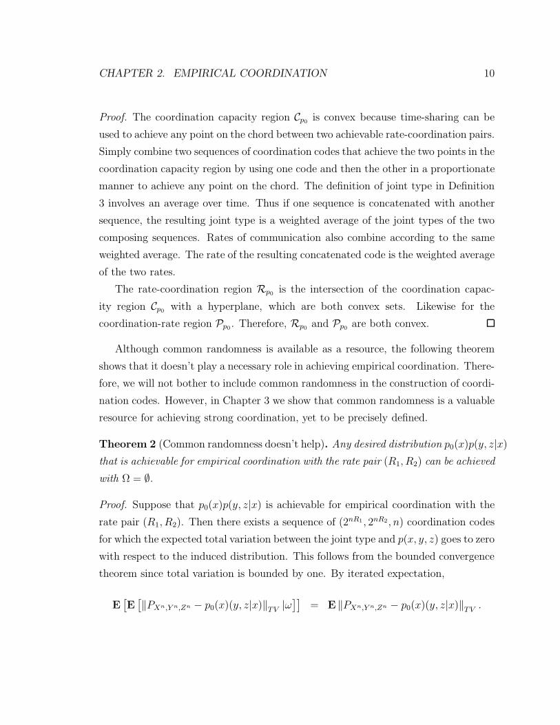
Figure 2.2: Shorthand notation for the cascade network of Figure 2.1.
action, and then from Node Y to Node Z at rate R2 bits per action.
Specifically, a (2nR1, 2nR2 , n) coordination code is used as a protocol to coordinate
the actions in the network for a block of n time periods. The coordination code and
the distribution of the random actions Xn induce a joint distribution on the actions
in the network. If the joint type of the actions in the network can be made arbitrarily
close to a desired distribution p0(x)p(y, z|x) with high probability, according to the
distribution induced by a (2nR1, 2nR2, n)) coordination code, then p0(x)p(y, z|x) is
achievable with the rate pair (R1, R2).
Definition 1 (Coordination code). A (2nR1 , 2nR2, n) coordination code for the cascade
network of Figure 2.1 consists of four functions—an encoding function
i : X n × Ω −→ 1, ..., 2nR1,
CHAPTER 2. EMPIRICAL COORDINATION 8
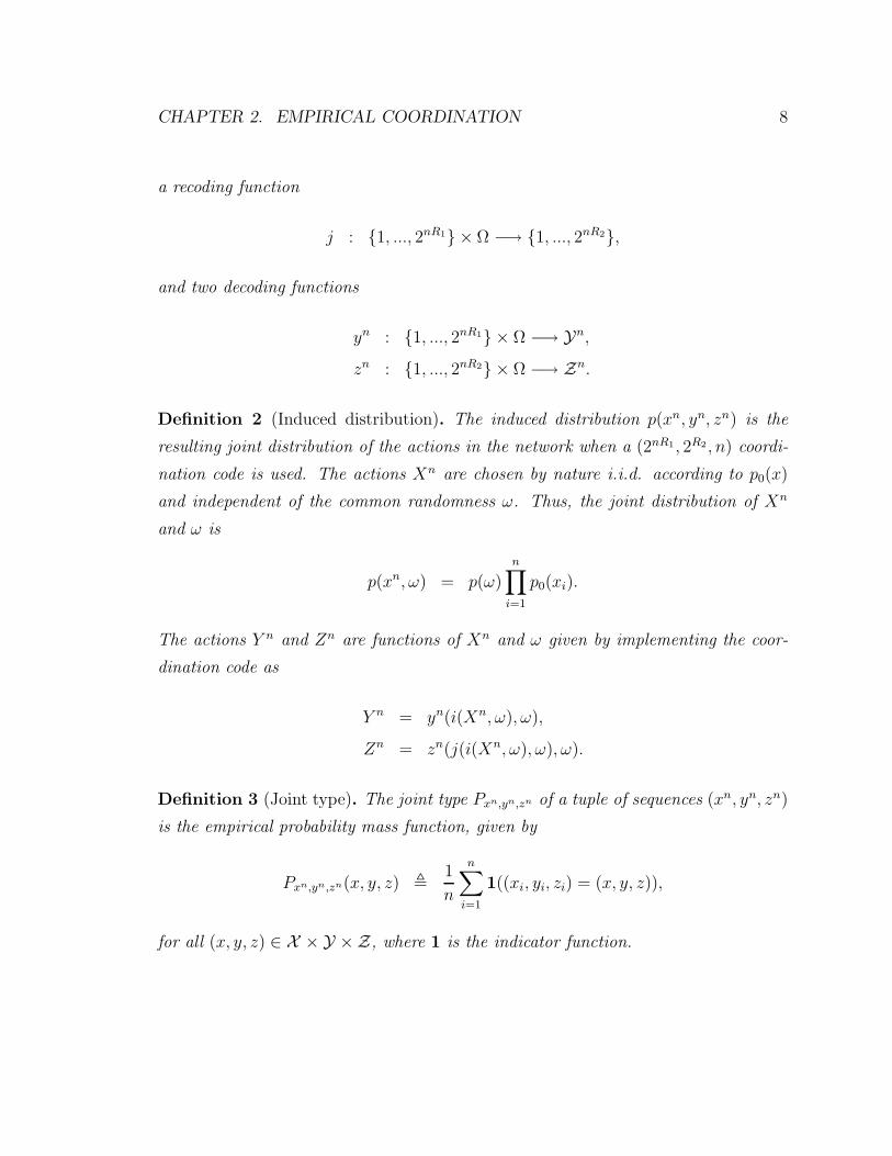
a recoding function
j : 1, ..., 2nR1 × Ω −→ 1, ..., 2nR2,
and two decoding functions
yn : 1, ..., 2nR1 × Ω −→ Yn,
zn : 1, ..., 2nR2 × Ω −→ Zn.
Definition 2 (Induced distribution). The induced distribution p(xn, yn, zn) is the
resulting joint distribution of the actions in the network when a (2nR1, 2R2 , n) coordi-
nation code is used. The actions Xn are chosen by nature i.i.d. according to p0(x)
and independent of the common randomness ω. Thus, the joint distribution of Xn
and ω is
p(xn, ω) = p(ω)
n∏
i=1
p0(xi).
The actions Y n and Zn are functions of Xn and ω given by implementing the coor-
dination code as
Y n = yn(i(Xn, ω), ω),
Zn = zn(j(i(Xn, ω), ω), ω).
Definition 3 (Joint type). The joint type Pxn,yn,zn of a tuple of sequences (xn, yn, zn)
is the empirical probability mass function, given by
Pxn,yn,zn(x, y, z) ,1
n
n∑
i=1
1((xi, yi, zi) = (x, y, z)),
for all (x, y, z) ∈ X × Y ×Z, where 1 is the indicator function.
CHAPTER 2. EMPIRICAL COORDINATION 9
Definition 4 (Total variation). The total variation between two probability mass
functions is half the L1 distance between them, given by
‖p(x, y, z) − q(x, y, z)‖TV ,1
2
∑
x,y,z
|p(x, y, z) − q(x, y, z)|.
Definition 5 (Achievability). A desired distribution p0(x)p(y, z|x) is achievable with
the rate pair (R1, R2) if there exists a sequence of (2nR1, 2nR2, n) coordination codes
and a choice of p(ω) such that under the induced distribution the total variation
between the joint type of the actions in the network and the desired distribution goes
to zero in probability. That is,
‖PXn,Y n,Zn(x, y, z) − p0(x)p(y, z|x)‖TV −→ 0 in probability.
Definition 6 (Coordination capacity region). The coordination capacity region Cp0
for the source distribution p0(x) is the closure of the set of rate-coordination tuples
(R1, R2, p(y, z|x)) that are achievable:
Cp0 , Cl
(R1, R2, p(y, z|x)) :
p0(x)p(y, z|x) is achievable at rates (R1, R2)
.
Definition 7 (Rate-coordination region). The rate-coordination region Rp0 is a slice
of the coordination capacity region corresponding to a fixed distribution p(y, z|x):
Rp0(p(y, z|x)) , (R1, R2) : (R1, R2, p(y, z|x)) ∈ Cp0.
Definition 8 (Coordination-rate region). The coordination-rate region Pp0 is a slice
of the coordination capacity region corresponding to a tuple of rates (R1, R2):
Pp0(R1, R2) , p(y, z|x) : (R1, R2, p(y, z|x)) ∈ Cp0.
2.1.1 Preliminary observations
Lemma 1 (Convexity of coordination). Cp0, Rp0, and Pp0 are all convex sets.
CHAPTER 2. EMPIRICAL COORDINATION 10
Proof. The coordination capacity region Cp0 is convex because time-sharing can be
used to achieve any point on the chord between two achievable rate-coordination pairs.
Simply combine two sequences of coordination codes that achieve the two points in the
coordination capacity region by using one code and then the other in a proportionate
manner to achieve any point on the chord. The definition of joint type in Definition
3 involves an average over time. Thus if one sequence is concatenated with another
sequence, the resulting joint type is a weighted average of the joint types of the two
composing sequences. Rates of communication also combine according to the same
weighted average. The rate of the resulting concatenated code is the weighted average
of the two rates.
The rate-coordination region Rp0 is the intersection of the coordination capac-
ity region Cp0 with a hyperplane, which are both convex sets. Likewise for the
coordination-rate region Pp0 . Therefore, Rp0 and Pp0 are both convex.
Although common randomness is available as a resource, the following theorem
shows that it doesn’t play a necessary role in achieving empirical coordination. There-
fore, we will not bother to include common randomness in the construction of coordi-
nation codes. However, in Chapter 3 we show that common randomness is a valuable
resource for achieving strong coordination, yet to be precisely defined.
Theorem 2 (Common randomness doesn’t help). Any desired distribution p0(x)p(y, z|x)
that is achievable for empirical coordination with the rate pair (R1, R2) can be achieved
with Ω = ∅.
Proof. Suppose that p0(x)p(y, z|x) is achievable for empirical coordination with the
rate pair (R1, R2). Then there exists a sequence of (2nR1, 2nR2, n) coordination codes
for which the expected total variation between the joint type and p(x, y, z) goes to zero
with respect to the induced distribution. This follows from the bounded convergence
theorem since total variation is bounded by one. By iterated expectation,
E[E[‖PXn,Y n,Zn − p0(x)(y, z|x)‖TV |ω
]]= E ‖PXn,Y n,Zn − p0(x)(y, z|x)‖TV .
CHAPTER 2. EMPIRICAL COORDINATION 11
Therefore, there exists a value ω∗ such that
E[‖PXn,Y n,Zn − p0(x)(y, z|x)‖TV |ω∗] ≤ E ‖PXn,Y n,Zn − p0(x)(y, z|x)‖TV .
Define a new coordination code that doesn’t depend on ω and at the same time
doesn’t increase the expected total variation:
i∗(xn) = i(xn, ω∗),
j∗(i) = j(i, ω∗),
yn∗(i) = Y n(i, ω∗),
zn∗(j) = Zn(j, ω∗).
This can be done for each (2nR1, 2nR2 , n) coordination code for n = 1, 2, ....
2.1.2 Generalize
We will investigate empirical coordination in a variety of networks. In each case, we
explicitly specify the structure and implementation of the coordination codes, similar
to Definitions 1 and 2, while all other definitions carry over in a straightforward
manner.
We use a shorthand notation in order to illustrate each network setting with a
simple and consistent figure. Figure 2.2 shows the shorthand notation for the cascade
network of Figure 2.1. The random actions that are specified by nature are shown with
arrows pointing down toward the node (represented by a block). Actions constructed
by the nodes themselves are shown coming out of the node with an arrow downward.
And arrows indicating communication from one node to another are labeled with the
rate limits for the communication along those links.
We fully characterize the coordination capacity regions Cp0 for empirical coordi-
nation in four network settings: a network of two nodes (Section 2.2.1); an isolated
node network (Section 2.2.2); a cascade network (Section 2.2.3); and a degraded
source network (Section 2.2.4). Additionally, we give bounds on the coordination
capacity region in two more network settings: a broadcast network (Section 2.2.5);
CHAPTER 2. EMPIRICAL COORDINATION 12
and a cascade multiterminal network (Section 2.2.5). Proofs are left to Section 2.4.
A communication technique that we find useful in several settings is to use a por-
tion of the communication to send identical messages to all nodes in the network. The
common message serves to correlate the codebooks used on different communication
links and can result in reduced rates in the network.
2.2 Network results
2.2.1 Two nodes
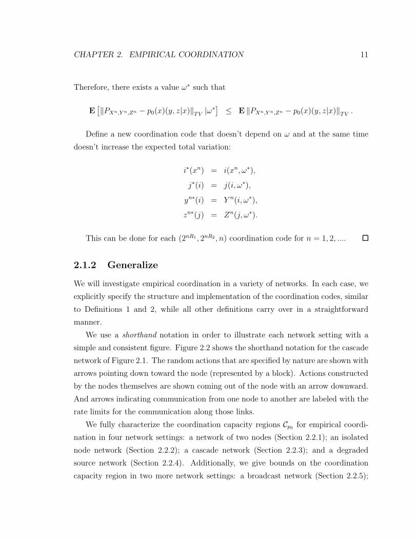
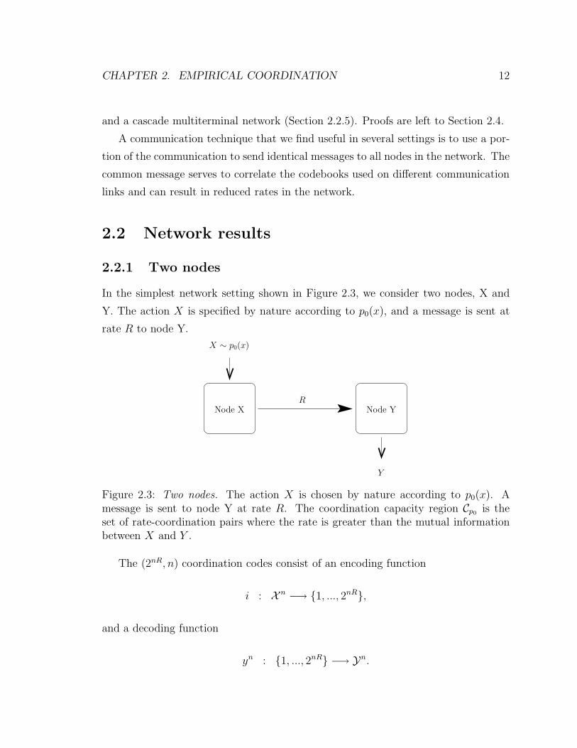
In the simplest network setting shown in Figure 2.3, we consider two nodes, X and
Y. The action X is specified by nature according to p0(x), and a message is sent at
rate R to node Y.
X ∼ p0(x)
Y
RNode X Node Y
Figure 2.3: Two nodes. The action X is chosen by nature according to p0(x). Amessage is sent to node Y at rate R. The coordination capacity region Cp0 is theset of rate-coordination pairs where the rate is greater than the mutual informationbetween X and Y .
The (2nR, n) coordination codes consist of an encoding function
i : X n −→ 1, ..., 2nR,
and a decoding function
yn : 1, ..., 2nR −→ Yn.
CHAPTER 2. EMPIRICAL COORDINATION 13
The actions Xn are chosen by nature i.i.d. according to p0(x), and the actions Y n
are functions of Xn given by implementing the coordination code as
Y n = yn(i(Xn)).
Theorem 3 (Coordination capacity region). The coordination capacity region Cp0
for empirical coordination in the two-node network of Figure 2.3 is the set of rate-
coordination pairs where the rate is greater than the mutual information between X
and Y . Thus,
Cp0 =
(R, p(y|x)) : R ≥ I(X; Y )
.
Discussion: The coordination capacity region in this setting yields the rate-
distortion result of Shannon [14].
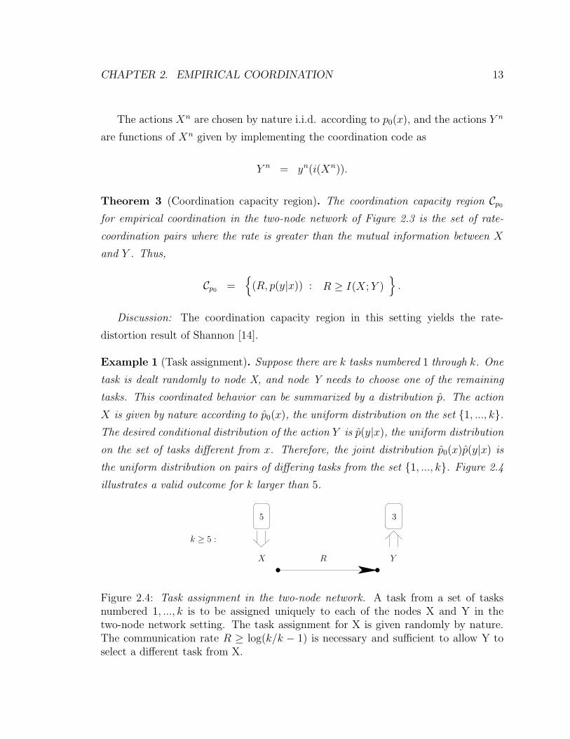
Example 1 (Task assignment). Suppose there are k tasks numbered 1 through k. One
task is dealt randomly to node X, and node Y needs to choose one of the remaining
tasks. This coordinated behavior can be summarized by a distribution p. The action
X is given by nature according to p0(x), the uniform distribution on the set 1, ..., k.The desired conditional distribution of the action Y is p(y|x), the uniform distribution
on the set of tasks different from x. Therefore, the joint distribution p0(x)p(y|x) is
the uniform distribution on pairs of differing tasks from the set 1, ..., k. Figure 2.4
illustrates a valid outcome for k larger than 5.
X YR
k ≥ 5 :
5 3
Figure 2.4: Task assignment in the two-node network. A task from a set of tasksnumbered 1, ..., k is to be assigned uniquely to each of the nodes X and Y in thetwo-node network setting. The task assignment for X is given randomly by nature.The communication rate R ≥ log(k/k − 1) is necessary and sufficient to allow Y toselect a different task from X.
CHAPTER 2. EMPIRICAL COORDINATION 14
By applying Theorem 3, we find that the rate-coordination region Rp0(p(y|x)) is
given by
Rp0(p(y|x)) =
R : R ≥ log
(k
k − 1
).
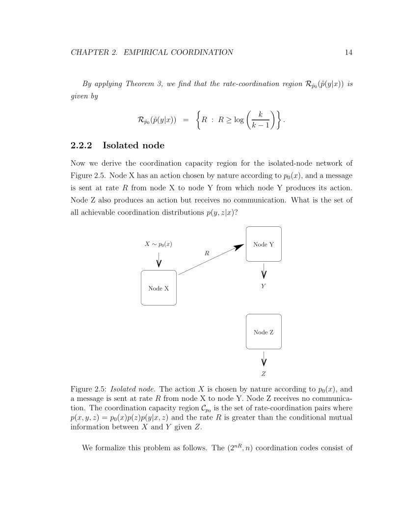
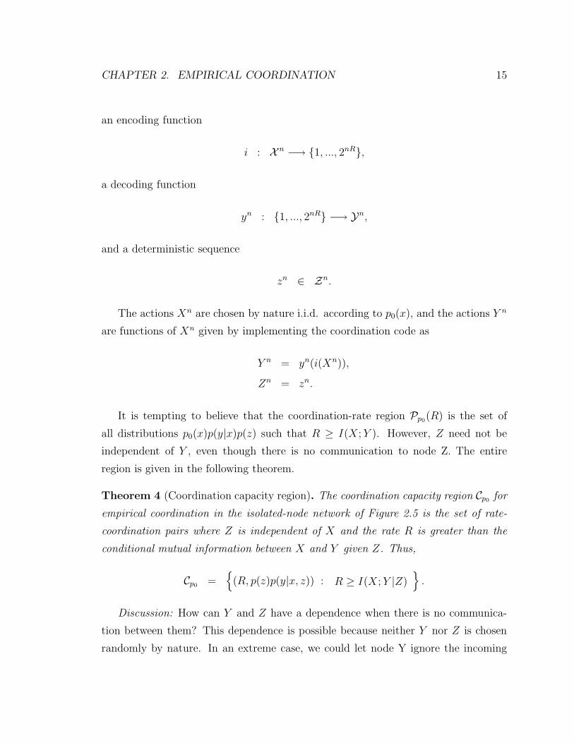
2.2.2 Isolated node
Now we derive the coordination capacity region for the isolated-node network of
Figure 2.5. Node X has an action chosen by nature according to p0(x), and a message
is sent at rate R from node X to node Y from which node Y produces its action.
Node Z also produces an action but receives no communication. What is the set of
all achievable coordination distributions p(y, z|x)?
X ∼ p0(x)
Y
Z
R
Node X
Node Y
Node Z
Figure 2.5: Isolated node. The action X is chosen by nature according to p0(x), anda message is sent at rate R from node X to node Y. Node Z receives no communica-tion. The coordination capacity region Cp0 is the set of rate-coordination pairs wherep(x, y, z) = p0(x)p(z)p(y|x, z) and the rate R is greater than the conditional mutualinformation between X and Y given Z.
We formalize this problem as follows. The (2nR, n) coordination codes consist of
CHAPTER 2. EMPIRICAL COORDINATION 15
an encoding function
i : X n −→ 1, ..., 2nR,
a decoding function
yn : 1, ..., 2nR −→ Yn,
and a deterministic sequence
zn ∈ Zn.
The actions Xn are chosen by nature i.i.d. according to p0(x), and the actions Y n
are functions of Xn given by implementing the coordination code as
Y n = yn(i(Xn)),
Zn = zn.
It is tempting to believe that the coordination-rate region Pp0(R) is the set of
all distributions p0(x)p(y|x)p(z) such that R ≥ I(X; Y ). However, Z need not be
independent of Y , even though there is no communication to node Z. The entire
region is given in the following theorem.
Theorem 4 (Coordination capacity region). The coordination capacity region Cp0 for
empirical coordination in the isolated-node network of Figure 2.5 is the set of rate-
coordination pairs where Z is independent of X and the rate R is greater than the
conditional mutual information between X and Y given Z. Thus,
Cp0 =
(R, p(z)p(y|x, z)) : R ≥ I(X; Y |Z)
.
Discussion: How can Y and Z have a dependence when there is no communica-
tion between them? This dependence is possible because neither Y nor Z is chosen
randomly by nature. In an extreme case, we could let node Y ignore the incoming
CHAPTER 2. EMPIRICAL COORDINATION 16
message from node X and let the actions at node Y and node Z be equal, Y = Z.
Thus we can immediately see that with no communication the coordination region
consists of all distributions of the form p0(x)p(y, z).
It is interesting to note that there is a tension between the correlation of X and Y
and the correlation of Y and Z. For instance, if the communication is used to make
perfect correlation between X and Y then any potential correlation between Y and
Z is forfeited.
Within the results for the more general cascade network in the sequel (Section
2.2.3) we will find that Theorem 4 is an immediate consequence of Theorem 5 by
letting R2 = 0.
Example 2 (Jointly Gaussian). Jointly Gaussian distributions illustrate the tradeoff
between the correlation of X and Y and the correlation of Y and Z in the isolated-node
network. Consider the portion of the coordination-rate region Pp0(R) that consists of
jointly Gaussian distributions. If X is distributed according to N(0, σ2X), what set of
covariance matrices can be achieved at rate R?
So far we have discussed coordination for distribution functions with finite alpha-
bets. Extending to infinite alphabet distributions, achievability means that any finite
quantization of the joint distribution is achievable.
Using Theorem 4, we bound the correlations as follows:
R ≥ I(X; Y |Z)
= I(X; Y, Z)
=1
2log
|Kx||Kyz||KXY Z |
(a)=
1
2log
σ2x(σ
2yσ
2z − σ2
yz)
σ2xσ
2yσ
2z − σ2
xσ2yz − σ2
zσ2xy
(b)=
1
2log
1 −(
σyz
σyσz
)2
1 −(
σyz
σyσz
)2
−(
σxy
σxσy
)2
=1
2log
1 − ρ2yz
1 − ρ2yz − ρ2
xy
, (2.1)
CHAPTER 2. EMPIRICAL COORDINATION 17
where ρxy and ρyz are correlation coefficients. Equality (a) holds because σxz = 0 due
to the independence between X and Z. Obtain equality (b) by dividing the numerator
and denominator of the argument of the log by σ2xσ
2yσ
2z .
Unfolding (2.1) yields a linear tradeoff between the ρ2xy and ρ2
yz, given by
(1 − 2−2R)−1ρ2xy + ρ2
yz ≤ 1.
Thus any correlation coefficients ρxy and ρyz are achievable at rate R if they satisfy
the above constraint.
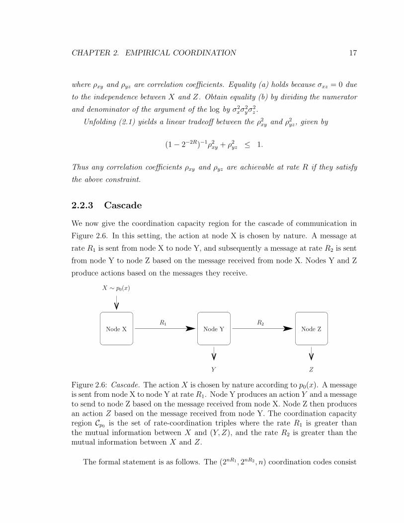
2.2.3 Cascade
We now give the coordination capacity region for the cascade of communication in
Figure 2.6. In this setting, the action at node X is chosen by nature. A message at
rate R1 is sent from node X to node Y, and subsequently a message at rate R2 is sent
from node Y to node Z based on the message received from node X. Nodes Y and Z
produce actions based on the messages they receive.
X ∼ p0(x)
Y Z
R1 R2
Node X Node Y Node Z
Figure 2.6: Cascade. The action X is chosen by nature according to p0(x). A messageis sent from node X to node Y at rate R1. Node Y produces an action Y and a messageto send to node Z based on the message received from node X. Node Z then producesan action Z based on the message received from node Y. The coordination capacityregion Cp0 is the set of rate-coordination triples where the rate R1 is greater thanthe mutual information between X and (Y, Z), and the rate R2 is greater than themutual information between X and Z.
The formal statement is as follows. The (2nR1, 2nR2, n) coordination codes consist
CHAPTER 2. EMPIRICAL COORDINATION 18
of four functions—an encoding function
i : X n −→ 1, ..., 2nR1,
a recoding function
j : 1, ..., 2nR1 −→ 1, ..., 2nR2,
and two decoding functions
yn : 1, ..., 2nR1 −→ Yn,
zn : 1, ..., 2nR2 −→ Zn.
The actions Xn are chosen by nature i.i.d. according to p0(x), and the actions Y n
and Zn are functions of Xn given by implementing the coordination code as
Y n = yn(i(Xn)),
Zn = zn(j(i(Xn))).
This network was considered by Yamamoto [15] in the context of rate-distortion
theory. The same optimal encoding scheme from his work achieves the coordination
capacity region as well.
Theorem 5 (Coordination capacity region). The coordination capacity region Cp0
for empirical coordination in the cascade network of Figure 2.6 is the set of rate-
coordination triples where the rate R1 is greater than the mutual information between
X and (Y, Z), and the rate R2 is greater than the mutual information between X and
Z. Thus,
Cp0 =
(R1, R2, p(y, z|x)) :R1 ≥ I(X; Y, Z),
R2 ≥ I(X; Z).
.
CHAPTER 2. EMPIRICAL COORDINATION 19
Discussion: The coordination capacity region Cp0 meets the cut-set bound. The
trick to achieving this bound is to first specify Z and then specify Y conditioned on
Z.
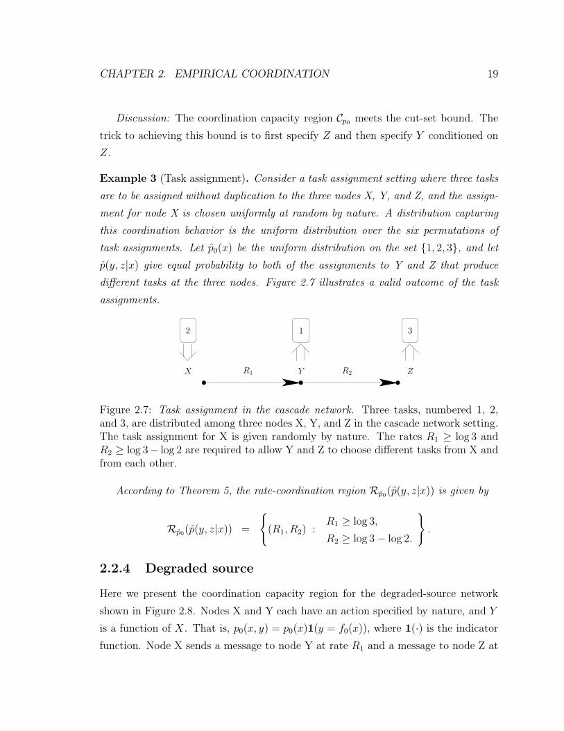
Example 3 (Task assignment). Consider a task assignment setting where three tasks
are to be assigned without duplication to the three nodes X, Y, and Z, and the assign-
ment for node X is chosen uniformly at random by nature. A distribution capturing
this coordination behavior is the uniform distribution over the six permutations of
task assignments. Let p0(x) be the uniform distribution on the set 1, 2, 3, and let
p(y, z|x) give equal probability to both of the assignments to Y and Z that produce
different tasks at the three nodes. Figure 2.7 illustrates a valid outcome of the task
assignments.
X Y ZR1 R2
2 1 3
Figure 2.7: Task assignment in the cascade network. Three tasks, numbered 1, 2,and 3, are distributed among three nodes X, Y, and Z in the cascade network setting.The task assignment for X is given randomly by nature. The rates R1 ≥ log 3 andR2 ≥ log 3− log 2 are required to allow Y and Z to choose different tasks from X andfrom each other.
According to Theorem 5, the rate-coordination region Rp0(p(y, z|x)) is given by
Rp0(p(y, z|x)) =
(R1, R2) :
R1 ≥ log 3,
R2 ≥ log 3 − log 2.
.
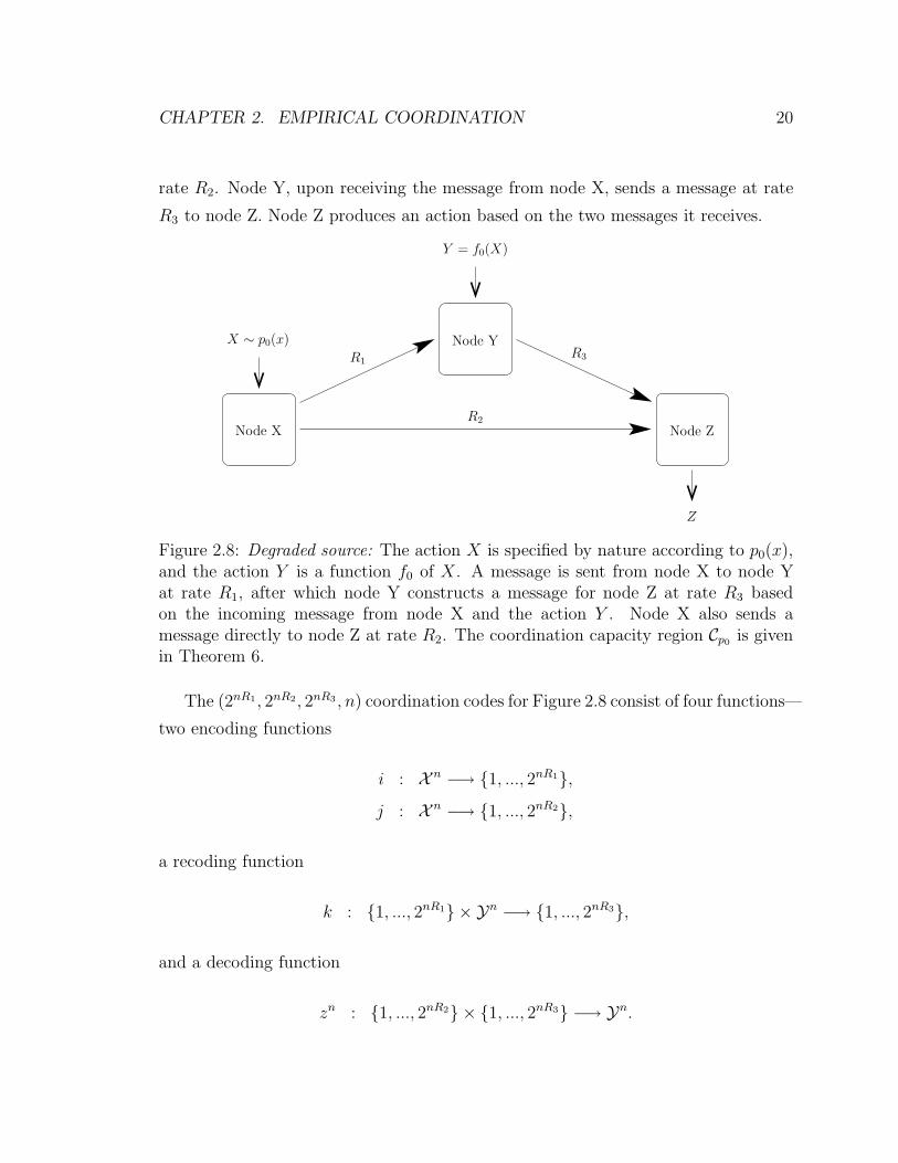
2.2.4 Degraded source
Here we present the coordination capacity region for the degraded-source network
shown in Figure 2.8. Nodes X and Y each have an action specified by nature, and Y
is a function of X. That is, p0(x, y) = p0(x)1(y = f0(x)), where 1(·) is the indicator
function. Node X sends a message to node Y at rate R1 and a message to node Z at
CHAPTER 2. EMPIRICAL COORDINATION 20
rate R2. Node Y, upon receiving the message from node X, sends a message at rate
R3 to node Z. Node Z produces an action based on the two messages it receives.
X ∼ p0(x)
Y = f0(X)
Z
R1R3
R2
Node X
Node Y
Node Z
Figure 2.8: Degraded source: The action X is specified by nature according to p0(x),and the action Y is a function f0 of X. A message is sent from node X to node Yat rate R1, after which node Y constructs a message for node Z at rate R3 basedon the incoming message from node X and the action Y . Node X also sends amessage directly to node Z at rate R2. The coordination capacity region Cp0 is givenin Theorem 6.
The (2nR1, 2nR2, 2nR3 , n) coordination codes for Figure 2.8 consist of four functions—
two encoding functions
i : X n −→ 1, ..., 2nR1,j : X n −→ 1, ..., 2nR2,
a recoding function
k : 1, ..., 2nR1 × Yn −→ 1, ..., 2nR3,
and a decoding function
zn : 1, ..., 2nR2 × 1, ..., 2nR3 −→ Yn.
CHAPTER 2. EMPIRICAL COORDINATION 21
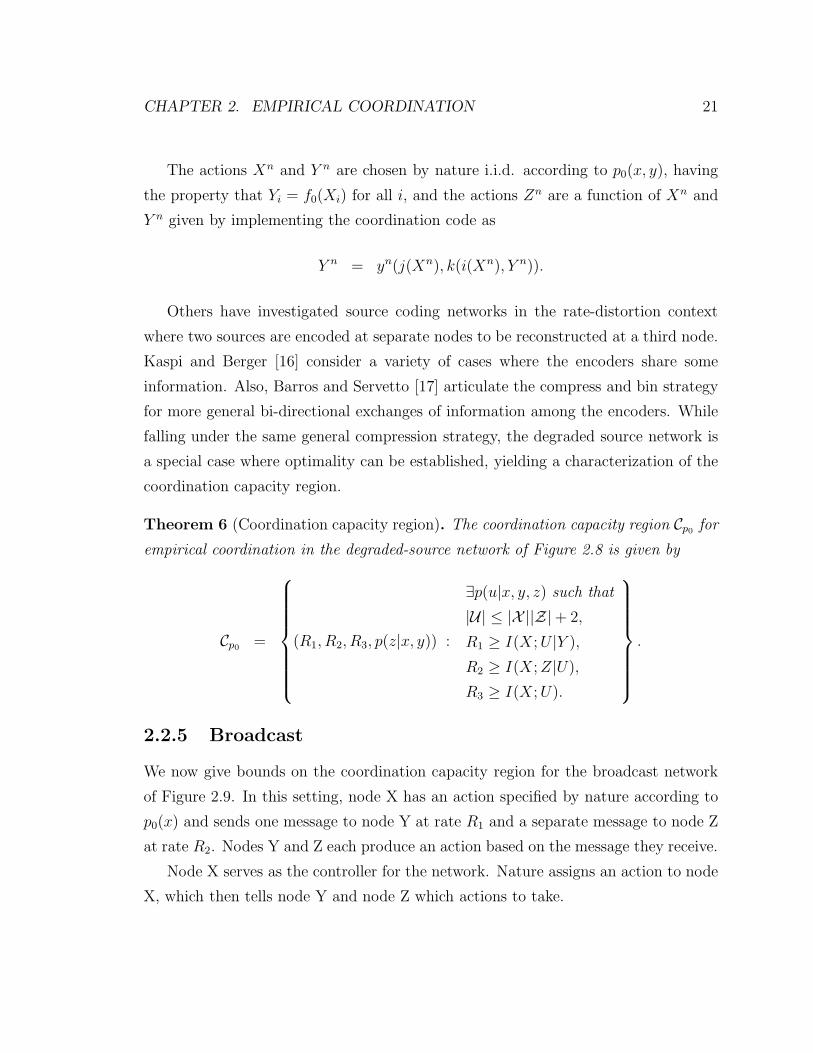
The actions Xn and Y n are chosen by nature i.i.d. according to p0(x, y), having
the property that Yi = f0(Xi) for all i, and the actions Zn are a function of Xn and
Y n given by implementing the coordination code as
Y n = yn(j(Xn), k(i(Xn), Y n)).
Others have investigated source coding networks in the rate-distortion context
where two sources are encoded at separate nodes to be reconstructed at a third node.
Kaspi and Berger [16] consider a variety of cases where the encoders share some
information. Also, Barros and Servetto [17] articulate the compress and bin strategy
for more general bi-directional exchanges of information among the encoders. While
falling under the same general compression strategy, the degraded source network is
a special case where optimality can be established, yielding a characterization of the
coordination capacity region.
Theorem 6 (Coordination capacity region). The coordination capacity region Cp0 for
empirical coordination in the degraded-source network of Figure 2.8 is given by
Cp0 =
(R1, R2, R3, p(z|x, y)) :
∃p(u|x, y, z) such that
|U| ≤ |X ||Z|+ 2,
R1 ≥ I(X; U |Y ),
R2 ≥ I(X; Z|U),
R3 ≥ I(X; U).
.
2.2.5 Broadcast
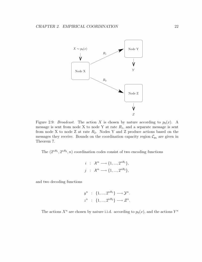
We now give bounds on the coordination capacity region for the broadcast network
of Figure 2.9. In this setting, node X has an action specified by nature according to
p0(x) and sends one message to node Y at rate R1 and a separate message to node Z
at rate R2. Nodes Y and Z each produce an action based on the message they receive.
Node X serves as the controller for the network. Nature assigns an action to node
X, which then tells node Y and node Z which actions to take.
CHAPTER 2. EMPIRICAL COORDINATION 22
X ∼ p0(x)
Y
Z
R1
R2
Node X
Node Y
Node Z
Figure 2.9: Broadcast. The action X is chosen by nature according to p0(x). Amessage is sent from node X to node Y at rate R1, and a separate message is sentfrom node X to node Z at rate R2. Nodes Y and Z produce actions based on themessages they receive. Bounds on the coordination capacity region Cp0 are given inTheorem 7.
The (2nR1, 2nR2, n) coordination codes consist of two encoding functions
i : X n −→ 1, ..., 2nR1,j : X n −→ 1, ..., 2nR2,
and two decoding functions
yn : 1, ..., 2nR1 −→ Yn.
zn : 1, ..., 2nR2 −→ Zn.
The actions Xn are chosen by nature i.i.d. according to p0(x), and the actions Y n
CHAPTER 2. EMPIRICAL COORDINATION 23
and Zn are functions of Xn given by implementing the coordination code as
Y n = yn(i(Xn)).
Zn = zn(j(Xn)).
From a rate-distortion point of view, the broadcast network is not a likely candi-
date for consideration. The problem separates into two non-interfering rate-distortion
problems, and the relationship between the sequences Y n and Zn is ignored. How-
ever, the problem of multiple descriptions, where the combination of two messages I
and J are used to make a third estimate of the source X, demands consideration of
the relationship between the two messages. In fact, the communication scheme for
the multiple descriptions problem presented by Zhang and Berger [18] coincides with
our inner bound for the coordination capacity region in the broadcast network.
The set of rate-coordination tuples Cp0,in is an inner bound on the coordination
capacity region, given by
Cp0,in ,
(R1, R2, p(y, z|x)) :
∃p(u|x, y, z) such that
R1 ≥ I(X; U, Y ),
R2 ≥ I(X; U, Z),
R1 + R2 ≥ I(X; U, Y ) + I(X; U, Z) + I(Y ; Z|X, U).
.
The set of rate-coordination tuples Cp0,out is an outer bound on the coordination
capacity region, given by
Cp0,out ,
(R1, R2, p(y, z|x)) :
R1 ≥ I(X; Y ),
R2 ≥ I(X; Z),
R1 + R2 ≥ I(X; Y, Z).
.
Also, define Rp0,in(p(y, z|x)) and Rp0,out(p(y, z|x)) to be the sets of rate pairs in Cp0,in
and Cp0,out corresponding to the desired distribution p(y, z|x).
CHAPTER 2. EMPIRICAL COORDINATION 24
Theorem 7 (Coordination capacity region bounds). The coordination capacity region
Cp0 for empirical coordination in the broadcast network of Figure 2.9 is bounded by
Cp0,in ⊂ Cp0 ⊂ Cp0,out.
Discussion: The regions Cp0,in and Cp0,out are convex. A time-sharing random
variable can be lumped into the auxiliary random variable U in the definition of Cp0,in
to show convexity.
The inner bound Cp0,in is achieved by first sending a common message, represented
by U , to both receivers and then private messages to each. The common message
effectively correlates the two codebooks to reduce the required rates for specifying the
actions Y n and Zn. The sum rate takes a penalty of I(Y ; Z|X, U) in order to assure
that Y and Z are coordinated with each other as well as with X.
The outer bound Cp0,out is a consequence of applying the two-node result of Theo-
rem 3 in three different ways, once for each receiver, and once for the pair of receivers
with full cooperation.
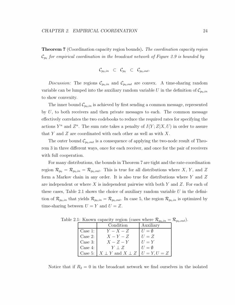
For many distributions, the bounds in Theorem 7 are tight and the rate-coordination
region Rp0 = Rp0,in = Rp0,out. This is true for all distributions where X, Y , and Z
form a Markov chain in any order. It is also true for distributions where Y and Z
are independent or where X is independent pairwise with both Y and Z. For each of
these cases, Table 2.1 shows the choice of auxiliary random variable U in the defini-
tion of Rp0,in that yields Rp0,in = Rp0,out. In case 5, the region Rp0,in is optimized by
time-sharing between U = Y and U = Z.
Table 2.1: Known capacity region (cases where Rp0,in = Rp0,out).Condition Auxiliary
Case 1: Y − X − Z U = ∅Case 2: X − Y − Z U = ZCase 3: X − Z − Y U = YCase 4: Y ⊥ Z U = ∅Case 5: X ⊥ Y and X ⊥ Z U = Y, U = Z
Notice that if R2 = 0 in the broadcast network we find ourselves in the isolated
CHAPTER 2. EMPIRICAL COORDINATION 25
node setting of Section 2.2.2. Consider a particular distribution p0(x)p(z)p(y|x, z)
that could be achieved in the isolated node network. In the setting of the broadcast
network, it might seem that the message from node X to node Z is useless for achieving
p0(x)p(z)p(y|x, z), since X and Z are independent. However, this is not the case.
For some desired distributions p0(x)p(z)p(y|x, z), a positive rate R2 in the broadcast
network actually helps reduce the required rate R1.
To highlight a specific case where a message to node Z is useful even though Z is in-
dependent of X in the desired distribution, consider the following. Let p0(x)p(z)p(y|x, z)
be the uniform distribution over all combinations of binary x, y, and z with even par-
ity. The variables X, Y , and Z are each Bernoulli-half and pairwise independent,
and X ⊕ Y ⊕ Z = 0, where ⊕ is addition modulo two. This distribution satisfies
both case 4 and case 5 from Table 2.1, so we know that Rp0= Rp0,out. Therefore, the
rate-coordination region Rp0(p(y, z|x)) is characterized by a single inequality,
Rp0(p(y, z|x)) = (R1, R2) ∈ R
2+ : R1 + R2 ≥ 1 bit.
The minimum rate R1 needed when no message is sent from node X to node Z is 1
bit, while the required rate in general is 1 − R2 bits.
Example 4 (Task assignment). Consider a task assignment setting similar to Exam-
ple 3, where three tasks are to be assigned without duplication to the three nodes X,
Y, and Z, and the assignment for node X is chosen uniformly at random by nature.
A distribution capturing this coordination behavior is the uniform distribution over
the six permutations of task assignments. Let p0(x) be the uniform distribution on
the set 0, 1, 2, and let p(y, z|x) give equal probability to both of the assignments to
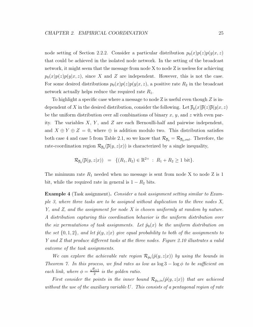
Y and Z that produce different tasks at the three nodes. Figure 2.10 illustrates a valid
outcome of the task assignments.
We can explore the achievable rate region Rp0(p(y, z|x)) by using the bounds in
Theorem 7. In this process, we find rates as low as log 3 − log φ to be sufficient on
each link, where φ =√
5+12
is the golden ratio.
First consider the points in the inner bound Rp0,in(p(y, z|x)) that are achieved
without the use of the auxiliary variable U . This consists of a pentagonal region of rate
CHAPTER 2. EMPIRICAL COORDINATION 26
X
Y
Z
R1
R2
1
0
2
Figure 2.10: Task assignment in the broadcast network. Three tasks, numbered 0,1, and 2, are distributed among three nodes X, Y, and Z in the broadcast networksetting. The task assignment for X is given randomly by nature. What rates R1 andR2 are necessary to allow Y and Z to choose different tasks from X and each other?
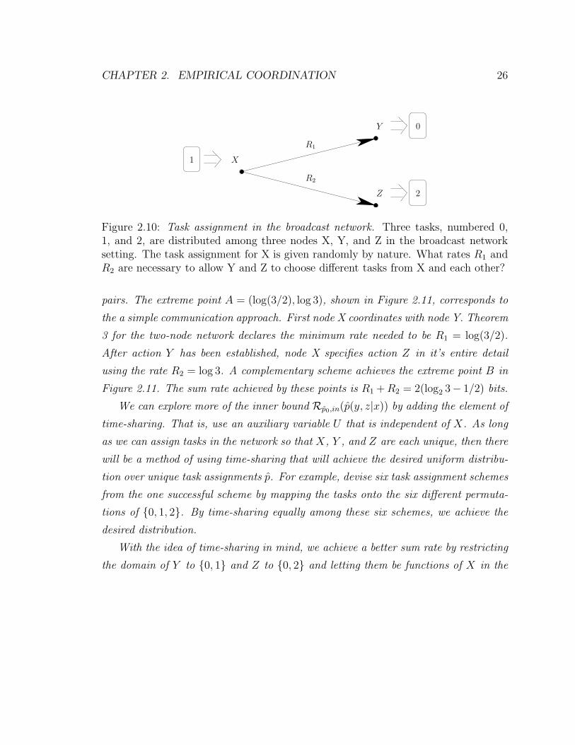
pairs. The extreme point A = (log(3/2), log 3), shown in Figure 2.11, corresponds to
the a simple communication approach. First node X coordinates with node Y. Theorem
3 for the two-node network declares the minimum rate needed to be R1 = log(3/2).
After action Y has been established, node X specifies action Z in it’s entire detail
using the rate R2 = log 3. A complementary scheme achieves the extreme point B in
Figure 2.11. The sum rate achieved by these points is R1 + R2 = 2(log2 3− 1/2) bits.
We can explore more of the inner bound Rp0,in(p(y, z|x)) by adding the element of
time-sharing. That is, use an auxiliary variable U that is independent of X. As long
as we can assign tasks in the network so that X, Y , and Z are each unique, then there
will be a method of using time-sharing that will achieve the desired uniform distribu-
tion over unique task assignments p. For example, devise six task assignment schemes
from the one successful scheme by mapping the tasks onto the six different permuta-
tions of 0, 1, 2. By time-sharing equally among these six schemes, we achieve the
desired distribution.
With the idea of time-sharing in mind, we achieve a better sum rate by restricting
the domain of Y to 0, 1 and Z to 0, 2 and letting them be functions of X in the
CHAPTER 2. EMPIRICAL COORDINATION 27
A
B
C
D
R1
R2
1
1
Figure 2.11: Rate region bounds for task assignment. Points A, B, C, and D areachievable rates for the task assignment problem in the broadcast network. The solidline indicates the outer bound Rp0,out(p(y, z|x)), and the dashed line indicates a subsetof the inner bound Rp0,in(p(y, z|x)). Points A and B are achieved by letting U = ∅.Point C uses U as time-sharing, independent of X. Point D uses U to describe Xpartially to each of the nodes Y and Z.
following way:
Y =
1, X 6= 1,
0, X = 1,(2.2)
Z =
2, X 6= 2,
0, X = 2.(2.3)
We can say that Y takes on a default value of 1, and Z takes on a default value of 2.
Node X just tells nodes Y and Z when they need to get out of the way, in which case
they switch to task 0. To achieve this we only need R1 ≥ H(Y ) = log3 −2/3 bits and
R2 ≥ H(Z) = log2 3 − 2/3 bits, represented by point C in Figure 2.11.
Finally, we achieve an even smaller sum rate in the inner bound Rp0,in(p(y, z|x))
CHAPTER 2. EMPIRICAL COORDINATION 28
by using a more interesting choice of U in addition to time-sharing.1 Let U ∈ 0, 1, 2be correlated with X in such a way that they are equal more often than one third of
the time. Now restrict the domains of Y and Z based on U . The actions Y and Z
are functions of X and U defined as follows:
Y =
U + 1 mod 3, X 6= U + 1 mod 3,
U, X = U + 1 mod 3,(2.4)
Z =
U − 1 mod 3, X 6= U − 1 mod 3,
U, X = U − 1 mod 3.(2.5)
This corresponds to sending a compressed description of X, represented by U , and
then assigning default values to Y and Z centered around U . The actions Y and Z
sit on both sides of U and only move when X tells them to get out of the way. The
description rates needed for this method are
R1 ≥ I(X; U) + I(X; Y |U)
= I(X; U) + H(Y |U).
R2 ≥ I(X; U) + I(X; Z|U)
= I(X; U) + H(Z|U). (2.6)
Using a symmetric conditional distribution from X to U , calculus provides the
following parameters:
P (U = u|X = x) =
1√5, u = x,
1φ√
5, u 6= x,
(2.7)
(2.8)
where φ =√
5+12
is the golden ratio. This level of compression results in a very low
rate of description, I(X; U) ≈ 0.04 bits, for sending U to each of the nodes Y and Z.
The description rates needed for this method are as follows, and are represented
1Time-sharing is also lumped into U , but we ignore that here to simplify the explanation.
CHAPTER 2. EMPIRICAL COORDINATION 29
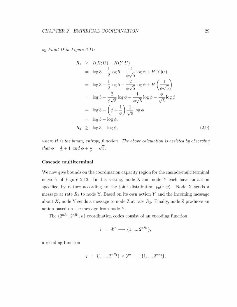
by Point D in Figure 2.11:
R1 ≥ I(X; U) + H(Y |U)
= log 3 − 1
2log 5 − 2
φ√
5log φ + H(Y |U)
= log 3 − 1
2log 5 − 2
φ√
5log φ + H
(1
φ√
5
)
= log 3 − 2
φ√
5log φ +
1
φ√
5log φ − φ√
5log φ
= log 3 −(
φ +1
φ
)1√5
log φ
= log 3 − log φ,
R2 ≥ log 3 − log φ, (2.9)
where H is the binary entropy function. The above calculation is assisted by observing
that φ = 1φ
+ 1 and φ + 1φ
=√
5.
Cascade multiterminal
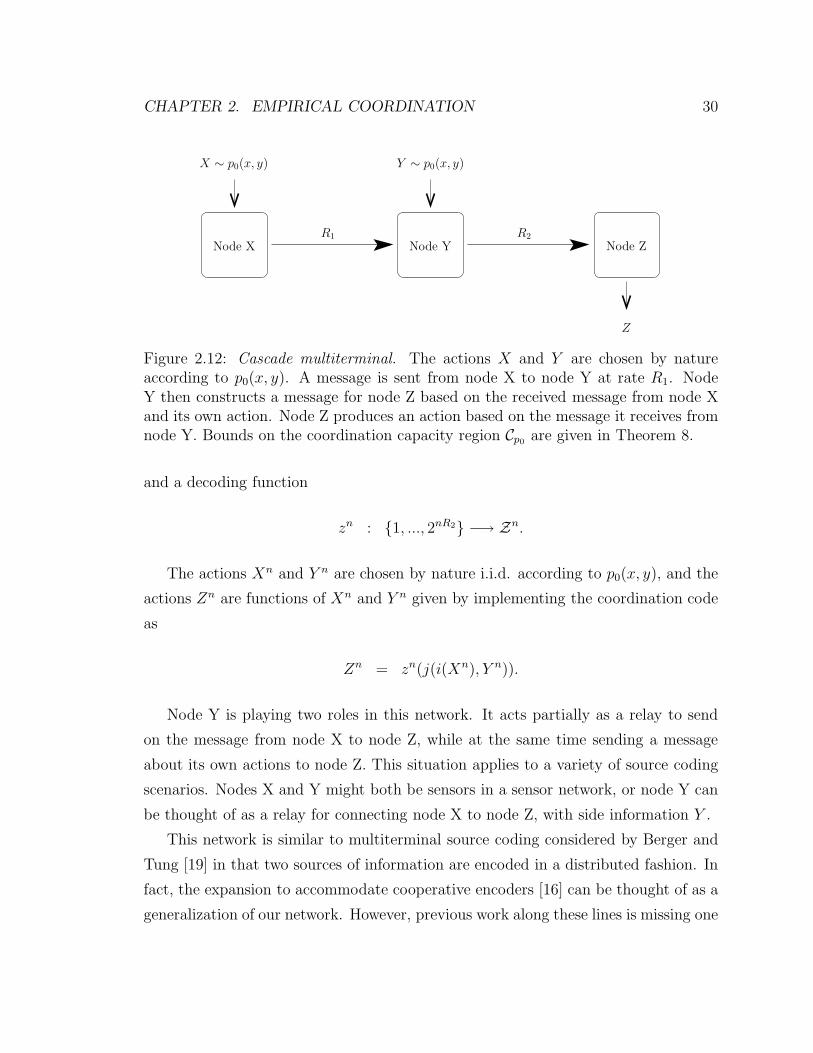
We now give bounds on the coordination capacity region for the cascade-multiterminal
network of Figure 2.12. In this setting, node X and node Y each have an action
specified by nature according to the joint distribution p0(x, y). Node X sends a
message at rate R1 to node Y. Based on its own action Y and the incoming message
about X, node Y sends a message to node Z at rate R2. Finally, node Z produces an
action based on the message from node Y.
The (2nR1, 2nR2, n) coordination codes consist of an encoding function
i : X n −→ 1, ..., 2nR1,
a recoding function
j : 1, ..., 2nR1 × Yn −→ 1, ..., 2nR2,
CHAPTER 2. EMPIRICAL COORDINATION 30
X ∼ p0(x, y) Y ∼ p0(x, y)
Z
R1 R2
Node X Node Y Node Z
Figure 2.12: Cascade multiterminal. The actions X and Y are chosen by natureaccording to p0(x, y). A message is sent from node X to node Y at rate R1. NodeY then constructs a message for node Z based on the received message from node Xand its own action. Node Z produces an action based on the message it receives fromnode Y. Bounds on the coordination capacity region Cp0 are given in Theorem 8.
and a decoding function
zn : 1, ..., 2nR2 −→ Zn.
The actions Xn and Y n are chosen by nature i.i.d. according to p0(x, y), and the
actions Zn are functions of Xn and Y n given by implementing the coordination code
as
Zn = zn(j(i(Xn), Y n)).
Node Y is playing two roles in this network. It acts partially as a relay to send
on the message from node X to node Z, while at the same time sending a message
about its own actions to node Z. This situation applies to a variety of source coding
scenarios. Nodes X and Y might both be sensors in a sensor network, or node Y can
be thought of as a relay for connecting node X to node Z, with side information Y .
This network is similar to multiterminal source coding considered by Berger and
Tung [19] in that two sources of information are encoded in a distributed fashion. In
fact, the expansion to accommodate cooperative encoders [16] can be thought of as a
generalization of our network. However, previous work along these lines is missing one
CHAPTER 2. EMPIRICAL COORDINATION 31
key aspect of efficiency, which is to partially relay the encoded information without
changing it.
Vasudevan, Tian, and Diggavi [20] looked at a similar cascade communication
system with a relay. In their setting, the relay’s information Y is a degraded version
of the decoder’s side information, and the decoder is only interested in recovering X.
Because the relays observations contain no additional information for the decoder,
the relay does not face the dilemma of mixing in some of the side information into its
outgoing message. In our cascade multiterminal network, the decoder does not have
side information. Thus, the relay is faced with coalescing the two pieces of information
X and Y into a single message. Other research involving similar network settings can
be found in [21], where Gu and Effros consider a more general network but with the
restriction that the action Y is a function of the action X, and [22], where Bakshi et.
al. identify the optimal rate region for lossless encoding of independent sources in a
longer cascade (line) network.
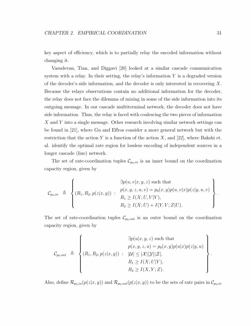
The set of rate-coordination tuples Cp0,in is an inner bound on the coordination
capacity region, given by
Cp0,in ,
(R1, R2, p(z|x, y)) :
∃p(u, v|x, y, z) such that
p(x, y, z, u, v) = p0(x, y)p(u, v|x)p(z|y, u, v)
R1 ≥ I(X; U, V |Y ),
R2 ≥ I(X; U) + I(Y, V ; Z|U).
.
The set of rate-coordination tuples Cp0,out is an outer bound on the coordination
capacity region, given by
Cp0,out ,
(R1, R2, p(z|x, y)) :
∃p(u|x, y, z) such that
p(x, y, z, u) = p0(x, y)p(u|x)p(z|y, u)
|U| ≤ |X ||Y||Z|,R1 ≥ I(X; U |Y ),
R2 ≥ I(X, Y ; Z).
.
Also, define Rp0,in(p(z|x, y)) and Rp0,out(p(z|x, y)) to be the sets of rate pairs in Cp0,in
CHAPTER 2. EMPIRICAL COORDINATION 32
and Cp0,out corresponding to the desired distribution p(z|x, y).
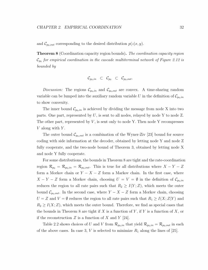
Theorem 8 (Coordination capacity region bounds). The coordination capacity region
Cp0 for empirical coordination in the cascade multiterminal network of Figure 2.12 is
bounded by
Cp0,in ⊂ Cp0 ⊂ Cp0,out.
Discussion: The regions Cp0,in and Cp0,out are convex. A time-sharing random
variable can be lumped into the auxiliary random variable U in the definition of Cp0,in
to show convexity.
The inner bound Cp0,in is achieved by dividing the message from node X into two
parts. One part, represented by U , is sent to all nodes, relayed by node Y to node Z.
The other part, represented by V , is sent only to node Y. Then node Y recompresses
V along with Y .
The outer bound Cp0,out is a combination of the Wyner-Ziv [23] bound for source
coding with side information at the decoder, obtained by letting node Y and node Z
fully cooperate, and the two-node bound of Theorem 3, obtained by letting node X
and node Y fully cooperate.
For some distributions, the bounds in Theorem 8 are tight and the rate-coordination
region Rp0 = Rp0,in = Rp0,out. This is true for all distributions where X − Y − Z
form a Morkov chain or Y − X − Z form a Markov chain. In the first case, where
X − Y − Z form a Morkov chain, choosing U = V = ∅ in the definition of Cp0,in
reduces the region to all rate pairs such that R2 ≥ I(Y ; Z), which meets the outer
bound Cp0,out. In the second case, where Y − X − Z form a Morkov chain, choosing
U = Z and V = ∅ reduces the region to all rate pairs such that R1 ≥ I(X; Z|Y ) and
R2 ≥ I(X; Z), which meets the outer bound. Therefore, we find as special cases that
the bounds in Theorem 8 are tight if X is a function of Y , if Y is a function of X, or
if the reconstruction Z is a function of X and Y [24].
Table 2.2 shows choices of U and V from Rp0,in that yield Rp0,in = Rp0,out in each
of the above cases. In case 3, V is selected to minimize R1 along the lines of [25].
CHAPTER 2. EMPIRICAL COORDINATION 33
Table 2.2: Known capacity region (cases where Rp0,in = Rp0,out).Condition Auxiliary
Case 1: X − Y − Z U = ∅, V = ∅Case 2: Y − X − Z U = Z, V = ∅Case 3: Z = f(X, Y ) U = ∅
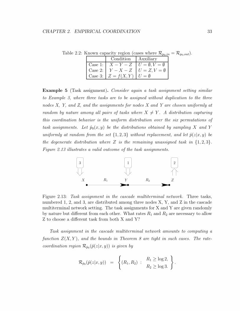
Example 5 (Task assignment). Consider again a task assignment setting similar
to Example 3, where three tasks are to be assigned without duplication to the three
nodes X, Y, and Z, and the assignments for nodes X and Y are chosen uniformly at
random by nature among all pairs of tasks where X 6= Y . A distribution capturing
this coordination behavior is the uniform distribution over the six permutations of
task assignments. Let p0(x, y) be the distributions obtained by sampling X and Y
uniformly at random from the set 1, 2, 3 without replacement, and let p(z|x, y) be
the degenerate distribution where Z is the remaining unassigned task in 1, 2, 3.Figure 2.13 illustrates a valid outcome of the task assignments.
X Y ZR1 R2
3 1 2
Figure 2.13: Task assignment in the cascade multiterminal network. Three tasks,numbered 1, 2, and 3, are distributed among three nodes X, Y, and Z in the cascademultiterminal network setting. The task assignments for X and Y are given randomlyby nature but different from each other. What rates R1 and R2 are necessary to allowZ to choose a different task from both X and Y?
Task assignment in the cascade multiterminal network amounts to computing a
function Z(X, Y ), and the bounds in Theorem 8 are tight in such cases. The rate-
coordination region Rp0(p(z|x, y)) is given by
Rp0(p(z|x, y)) =
(R1, R2) :
R1 ≥ log 2,
R2 ≥ log 3.
.
CHAPTER 2. EMPIRICAL COORDINATION 34
This is achieved by letting U = ∅ and V = X in the definition of Cp0,in. To show
that this region meets the outer bound Cp0,out, make the observation that I(X; U |Y ) ≥I(X; Z|Y ) in relation to the bound on R1, since X − (Y, U) − Z forms a Markov
chain.
2.3 Rate-distortion theory
The challenge of describing random sources of information with the fewest bits pos-
sible can be defined in a number of different ways. Traditionally, source coding in
networks follows the path of rate-distortion theory by establishing multiple distortion
penalties for the multiple sources and reconstructions in the network. Yet, fundamen-
tally, the rate-distortion problem is intimately connected to empirical coordination.
The basic result of rate-distortion theory for a single memoryless source states
that in order to achieve any desired distortion level you must find an appropriate
conditional distribution of the reconstruction X given the source X and then use a
communication rate larger than the mutual information I(X; X). This lends itself
to the interpretation that optimal encoding for a rate-distortion setting really comes
down to coordinating a reconstruction sequence with a source sequence according
to a selected joint distribution. Here we make that observation formal by showing
that in general, even in networks, the rate-distortion region is a projection of the
coordination capacity region.
The coordination capacity region Cp0 is a set of rate-coordination tuples. We
can express rate-coordination tuples as vectors. For example, in the cascade net-
work of Section 2.2.3 there are two rates R1 and R2. The actions in this network
are X, Y , and Z, where X is given by nature. Order the space X × Y × Z in a
sequence (x1, y1, z1), ..., (xm, ym, zm), where m = |X ||Y||Z|. The rate-coordination tu-
ples (R1, R2, p(y, z|x)) can be expressed as vectors [R1, R2, p(y1, z1|x1), ..., p(ym, zm|xm)]T .
The rate-distortion region Dp0 is the closure of the set of rate-distortion tuples that
are achievable in a network. We say that a distortion D is achievable if there exists a
rate-distortion code that gives an expected average distortion less than D, using d as
a distortion measurement. For example, in the cascade network of Section 2.2.3 we
CHAPTER 2. EMPIRICAL COORDINATION 35
might have two distortion functions: The function d1(x, y) measures the distortion
in the reconstruction at node Y; the function d2(x, y, z) evaluates distortion jointly
between the reconstructions at nodes Y and Z. The rate-distortion region Dp0 would
consist of tuples (R1, R2, D1, D2), which indicate that using rates R1 and R2 in the
network, a source distributed according to p0(x) can be encoded to achieve no more
than D1 expected average distortion as measured by d1 and D2 distortion as measured
by d2.
The relationship between the rate-distortion region Dp0 and the coordination ca-
pacity region Cp0 is that of a linear projection. Suppose we have multiple finite-valued
distortion functions d1, ..., dk. We construct a distortion matrix D using the same enu-
meration (x1, y1, z1), ..., (xm, ym, zm) of the space X ×Y ×Z as was used to vectorize
the tuples in Cp0 :
D ,
d1(x1, y1, z1)p0(x1) · · · d1(xm, ym, zm)p0(xm)...
......
dk(x1, y1, z1)p0(x1) · · · dk(xm, ym, zm)p0(xm)
.
The distortion matrix D is embedded in a block diagonal matrix A where the upper-
left block is the identity matrix I with the same dimension as the number of rates in
the network:
A ,
[I 0
0 D
].
Theorem 9 (Rate-distortion region). The rate-distortion region Dp0 for a memory-
less source with distribution p0 in any rate-limited network is a linear projection of
the coordination capacity region Cp0 by the matrix A,
Dp0 = A Cp0.
We treat the elements of Dp0 and Cp0 as vectors, as discussed, and the matrix multi-
plication by A is the standard set multiplication.
CHAPTER 2. EMPIRICAL COORDINATION 36
Discussion: The proof of Theorem 9 can be found in Section 2.4. Since the
coordination capacity region Cp0 is a convex set, the rate-distortion region Dp0 is also
a convex set.
Clearly we can use a coordination code to achieve the corresponding distortion in
a rate-distortion setting. But the theorem makes a stronger statement. It says that
there is not a more efficient way of satisfying distortion limits in any network setting
with memoryless sources than by using a code that produces the same joint type
for almost every observation of the sources. It is conceivable that a rate-distortion
code for a network setting would produce a variety of different joint types, each sat-
isfying the distortion limit, but varying depending on the particular source sequence
observed. However, given such a rate-distortion code, repeated uses will produce
a longer coordination code that consistently achieves coordination according to the
expected joint type. The expected joint type of a good rate-distortion code can be
shown to satisfy the distortion constraints.
0 0.5 10
0.5
1
P (Y = 1|X = 0)
P(Y
=1|
X=
1)
R = 0.1
d ≤ D
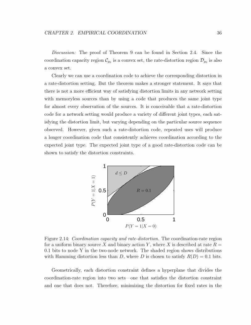
Figure 2.14: Coordination capacity and rate-distortion. The coordination-rate regionfor a uniform binary source X and binary action Y , where X is described at rate R =0.1 bits to node Y in the two-node network. The shaded region shows distributionswith Hamming distortion less than D, where D is chosen to satisfy R(D) = 0.1 bits.
Geometrically, each distortion constraint defines a hyperplane that divides the
coordination-rate region into two sets—one that satisfies the distortion constraint
and one that does not. Therefore, minimizing the distortion for fixed rates in the
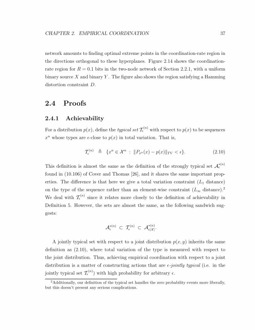
CHAPTER 2. EMPIRICAL COORDINATION 37
network amounts to finding optimal extreme points in the coordination-rate region in
the directions orthogonal to these hyperplanes. Figure 2.14 shows the coordination-
rate region for R = 0.1 bits in the two-node network of Section 2.2.1, with a uniform
binary source X and binary Y . The figure also shows the region satisfying a Hamming
distortion constraint D.
2.4 Proofs
2.4.1 Achievability
For a distribution p(x), define the typical set T (n)ǫ with respect to p(x) to be sequences
xn whose types are ǫ-close to p(x) in total variation. That is,
T (n)ǫ , xn ∈ X n : ‖Pxn(x) − p(x)‖TV < ǫ. (2.10)
This definition is almost the same as the definition of the strongly typical set A∗(n)ǫ
found in (10.106) of Cover and Thomas [26], and it shares the same important prop-
erties. The difference is that here we give a total variation constraint (L1 distance)
on the type of the sequence rather than an element-wise constraint (L∞ distance).2
We deal with T (n)ǫ since it relates more closely to the definition of achievability in
Definition 5. However, the sets are almost the same, as the following sandwich sug-
gests:
A∗(n)ǫ ⊂ T (n)
ǫ ⊂ A∗(n)ǫ|X | .
A jointly typical set with respect to a joint distribution p(x, y) inherits the same
definition as (2.10), where total variation of the type is measured with respect to
the joint distribution. Thus, achieving empirical coordination with respect to a joint
distribution is a matter of constructing actions that are ǫ-jointly typical (i.e. in the
jointly typical set T (n)ǫ ) with high probability for arbitrary ǫ.
2Additionally, our definition of the typical set handles the zero probability events more liberally,but this doesn’t present any serious complications.
CHAPTER 2. EMPIRICAL COORDINATION 38
Strong Markov lemma
The Markov Lemma [19] makes a statement about how likely a set of sequences will
be jointly typical with respect to a Markov chain given that adjacent pairs in the
chain are jointly typical. It is generally used to establish joint typicality in a source
coding scheme where side information is not known to the encoder. However, as the
network and encoding scheme become more intricate, the standard Markov Lemma
lacks the necessary strength. Here we introduce a generalization.3
Theorem 10 (Strong Markov lemma). Given a joint distribution p(x, y, z) on the
alphabet X × Y × Z that yields a Markov chain X − Y − Z (i.e. p(x, y, z) =
p(y)p(x|y)p(z|y)), let xn and yn be arbitrary sequences that are ǫ-jointly typical. Sup-
pose that Zn is chosen to be ǫ-jointly typical with yn and additionally has a distribution
that is permutation-invariant with respect to yn, which is to say, for all zn and zn,
Pyn,zn = Pyn,zn ⇒ P (Zn = zn) = P (Zn = zn). (2.11)
(Notice that this condition is commonly satisfied in a variety of random coding proof
techniques.) Then,
Pr((xn, yn, Zn) ∈ T (n)
4ǫ
)→ 1
exponentially fast as n goes to infinity.
Proof. The proof of Theorem 10 relies mainly on Lemma 11 (found in the sequel) and
the repeated use of the triangle inequality. Suppose that (2.12), the high probability
event of Lemma 11, holds true, namely
‖Pxn,yn,Zn − Pxn,ynPZn|yn‖TV < ǫ.
3Through conversation we discovered that similar effort is being made by Young-Han Kim andAbbas El Gamal and may shortly be found in the Stanford EE478 Lecture Notes.
CHAPTER 2. EMPIRICAL COORDINATION 39
By the definition of total variation one can easily show that
‖Pxn,ynPZn|yn − pX,Y PZn|yn‖TV = ‖Pxn,yn − pX,Y ‖TV
< ǫ.
Similarly,
‖pY pX|Y PZn|yn − PynpX|Y PZn|yn‖TV = ‖pY − Pyn‖TV
< ǫ.
And finally,
‖Pyn,ZnpX|Y − pX,Y,Z‖TV = ‖Pyn,Zn − pY,Z‖TV
< ǫ.
Thus, the triangle inequality gives
‖Pxn,yn,Zn − pX,Y,Z‖TV < 4ǫ.
Lemma 11 (Markov tendency). Let xn ∈ X n and yn ∈ Yn be arbitrary sequences.
Suppose that the random sequence Zn ∈ Zn has a distribution that is permutation-
invariant with respect to yn, as in (2.11). Then with high probability which only
depends on the sizes of the alphabets X , Y, and Z, the joint type Pxn,yn,Zn will be
ǫ-close to the Markov joint type. That is, for any ǫ > 0,
‖Pxn,yn,Zn − Pxn,ynPZn|yn‖TV < ǫ, (2.12)
with a probability of at least 1−2−αn+β log n, where α and β only depend on the alphabet
sizes and ǫ.
Proof. We start by defining two constants that simplify this discussion. The first
CHAPTER 2. EMPIRICAL COORDINATION 40
constant, α, is the key to obtaining the uniform bound that Lemma 11 provides.
α , minp(x,y,z)∈SX ,Y,Z : ‖p(x,y,z)−p(x,y)p(z|y)‖TV ≥ǫ
I(X; Z|Y ),
β , 2|X ||Y||Z|.
Here SX ,Y ,Z is the simplex with dimension corresponding to the product of the alpha-
bet sizes. Notice that α is defined as a minimization of a continuous function over a
compact set; therefore, by analysis we know that the minimum is achieved in the set.
Since I(X; Z|Y ) is positive for any distribution that does not form a Markov chain
X − Y −Z, we find that α is positive for ǫ > 0. The constants α and β are functions
of ǫ and the alphabet sizes |X |, |Y|, and |Z|.We categorize sequences into sets with the same joint type. The type class Tp(y,z)
is defined as
Tp(y,z) , (yn, zn) : Pyn,zn = p(y, z).
We also define a conditional type class Tp(z|y)(yn) to be the set of zn sequences such
that the pair (yn, zn) are in the type class Tp(y,z). Namely,
Tp(z|y)(yn) , zn : Pyn,zn = p(z|y)Pyn.
We will show that the statement made in (2.12) is true conditionally for each
conditional type class Tp(z|y)(yn) and therefore must be true overall.
Suppose Zn falls in the conditional type class TPzn|yn (yn). By assumption (2.11),
all zn in this type class are equally likely. Assessing probabilities simply becomes a
matter of counting. From the method of types [26] we know that
∣∣∣TPzn|yn (yn)∣∣∣ ≥ n−|Y||Z|2
nHPyn,zn (Z|Y ).
We also can bound the number of zn sequences in TPzn|yn (yn) that do not satisfy
CHAPTER 2. EMPIRICAL COORDINATION 41
(2.12). These sequences must fall in a conditional type class TPzn|xn,yn (xn, yn) where
∥∥Pxn,yn,zn − Pxn,ynPzn|yn
∥∥TV
≥ ǫ.
For each such type class, the size can be bounded by
∣∣∣TPzn|xn,yn (xn, yn)∣∣∣ ≤ 2
nHPxn,yn,zn (Z|X,Y )
= 2n(HPyn,zn (Z|Y )−IPxn,yn,zn (X;Z|Y )
)
≤ 2n(HPyn,zn (Z|Y )−α
)
.
Furthermore, there are only polynomially many types, bounded by n|X ||Y||Z|. There-
fore, the probability that Zn does not satisfy (2.12) for any Pzn|yn is bounded by
Pr( not (2.12) | Zn ∈ TPzn|yn (yn) ) =
∣∣∣zn ∈ TPzn|yn (yn) : not (2.12)∣∣∣
∣∣∣TPzn|yn (yn)∣∣∣
≤ n|X ||Y||Z|2n(HPyn,zn (Z|Y )−α
)
n−|Y||Z|2nHPyn,zn (Z|Y )
= n|Y||Z|+|X ||Y||Z|2−αn
≤ 2−αn+β log n.
Generic achievability proof
The coding techniques for achieving the empirical coordination regions in this chapter
are familiar from rate distortion theory. We construct random codebooks (based
on common randomness) and show that a particular randomized encoding scheme
performs well on average, resulting in jointly-typical actions with high probability.
Therefore, there must be at least one deterministic scheme that performs well. Here
we prove one generally useful example to verify that the rate-distortion techniques
actually do work for achieving empirical coordination.
CHAPTER 2. EMPIRICAL COORDINATION 42
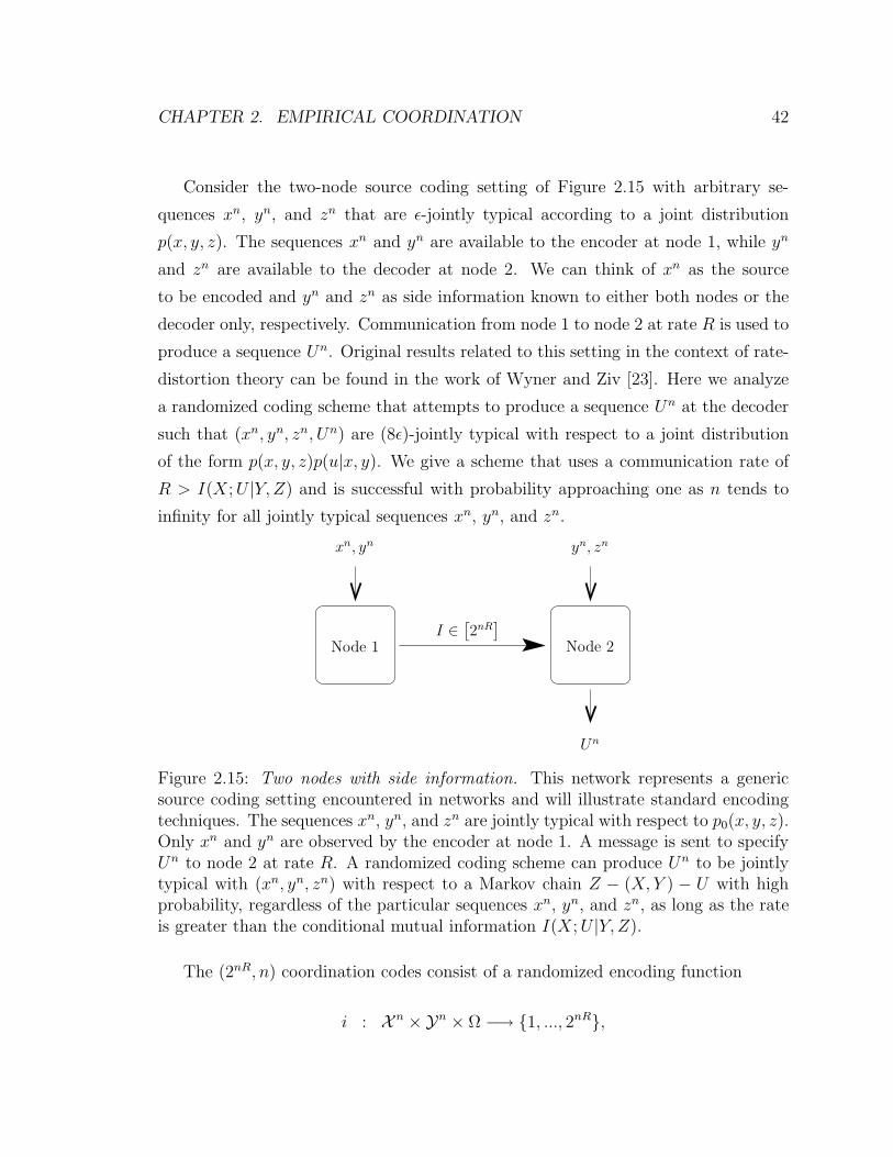
Consider the two-node source coding setting of Figure 2.15 with arbitrary se-
quences xn, yn, and zn that are ǫ-jointly typical according to a joint distribution
p(x, y, z). The sequences xn and yn are available to the encoder at node 1, while yn
and zn are available to the decoder at node 2. We can think of xn as the source
to be encoded and yn and zn as side information known to either both nodes or the
decoder only, respectively. Communication from node 1 to node 2 at rate R is used to
produce a sequence Un. Original results related to this setting in the context of rate-
distortion theory can be found in the work of Wyner and Ziv [23]. Here we analyze
a randomized coding scheme that attempts to produce a sequence Un at the decoder
such that (xn, yn, zn, Un) are (8ǫ)-jointly typical with respect to a joint distribution
of the form p(x, y, z)p(u|x, y). We give a scheme that uses a communication rate of
R > I(X; U |Y, Z) and is successful with probability approaching one as n tends to
infinity for all jointly typical sequences xn, yn, and zn.
xn, yn
Un
I ∈[2nR]
Node 1 Node 2
yn, zn
Figure 2.15: Two nodes with side information. This network represents a genericsource coding setting encountered in networks and will illustrate standard encodingtechniques. The sequences xn, yn, and zn are jointly typical with respect to p0(x, y, z).Only xn and yn are observed by the encoder at node 1. A message is sent to specifyUn to node 2 at rate R. A randomized coding scheme can produce Un to be jointlytypical with (xn, yn, zn) with respect to a Markov chain Z − (X, Y ) − U with highprobability, regardless of the particular sequences xn, yn, and zn, as long as the rateis greater than the conditional mutual information I(X; U |Y, Z).
The (2nR, n) coordination codes consist of a randomized encoding function
i : X n ×Yn × Ω −→ 1, ..., 2nR,
CHAPTER 2. EMPIRICAL COORDINATION 43
and a randomized decoding function
un : 1, ..., 2nR × Yn × Zn × Ω −→ Un.
These functions are random simply because the common randomness ω is involved
for generating random codebooks.
The sequences xn, yn, and zn are arbitrary jointly typical sequences according to
p0(x, y, z), and the sequence Un is a randomized function of xn, yn, and zn given by
implementing the coordination code as
Un = un(i(xn, yn, ω), yn, zn, ω).
Lemma 12 (Generic coordination with side information). For the two-node net-
work with side information of Figure 2.15 and any joint distribution of the form
p(x, y, z)p(u|x, y), a sequence of randomized coordination codes at rate R > I(X; U |Y, Z)
exists for which
Pr((xn, yn, zn, Un) ∈ T (n)
8ǫ
)→ 1
as n goes to infinity, uniformly for all (xn, yn, zn) ∈ T (n)ǫ .
Proof. Consider a joint distribution p(x, y, z)p(u|x, y) and a value of R such that
R − I(X; U |Y, Z) = γ > 0. We first over-cover the typical set of (xn, yn) using a
codebook of size 2nRc , where Rc = I(X, Y ; U) + γ/2. We then randomly categorize
the codebook sequences into 2nR bins, yielding 2nRb sequences in each bin, where
Rb = Rc − R
= I(X, Y ; U) − I(X; U |Y, Z) − γ/2
= I(X, Y, Z; U) − I(X; U |Y, Z) − γ/2
= I(Y, Z; U) − γ/2.
Codebook: Generate a codebook C of 2n(I(X;Z|U)−ǫ) sequences un(j) independently
CHAPTER 2. EMPIRICAL COORDINATION 44
according to the marginal distribution p(u), namely∏n
i=1 p(ui). Randomly and inde-
pendently assign each one a bin number b(un(j)) in the set 1, ..., 2nR.Encoder: The encoding function i(xn, yn, ω) can be explained as follows. Search
the codebook C and identify an index j such that (xn, yn, un(j)) ∈ T (n)2ǫ . If multiple
exist, select the first such j. If none exist, select j = 1. Send the bin number
i(xn, yn) = b(un(j)).
Decoder: The decoding function un(i, yn, zn, ω) can be explained as follows. Con-
sider the codebook C and identify an index j such that (yn, zn, un(j)) ∈ T (n)8ǫ and
b(un(j)) = i. If multiple exist, select the first such j. If none exist, select j = 1.
Produce the sequence Un = un(j).
Error Analysis: We conservatively declare errors for any of the following, E1, E2,
or E3.
Error 1: The encoder does not find a (2ǫ)-jointly typical sequence in the codebook.
By the method of types one can show, as in Lemma 10.6.2 of [26], that each sequence
in C is (2ǫ)-jointly typical with (xn, yn) with probability greater than 2−n(I(X,Y ;U)+δ(ǫ))
for n large enough, where δ(ǫ) goes to zero as ǫ goes to zero.
Each sequence in the codebook C is generated independently, so the probability
that none of them are jointly typical is bounded by
Pr(E1) ≤ (1 − 2−n(I(X,Y ;U)+δ(ǫ)))2nRc
≤ e−2nRc2−n(I(X,Y ;U)+δ(ǫ))
= e−2n(Rc−I(X,Y ;U)−δ(ǫ))
= e−2n(γ/2−δ(ǫ))
.
If ǫ is chosen small enough, this tends to zero as n tends to infinity.
Error 2: The sequence identified by the encoder is not (8ǫ)-jointly typical with
(xn, yn, zn). Assuming E1 did not occur, because of the Markovity Z − (X, Y ) − U
implied by p(x, y, z)p(u|x, y) and the symmetry of our codebook construction, we can
invoke Theorem 10 to verify that the conditional probability Pr(E2|Ec1) is arbitrarily
small for large enough n.
Error 3: The decoder finds more than one eligible action sequences. Assume that
CHAPTER 2. EMPIRICAL COORDINATION 45
E1 and E2 did not occur. If the decoder considers the same index j as the encoder
selected, then certainly un(j) will be be eligible, which is to say it will be (8ǫ)-jointly
typical with (yn, zn), and the bin index will match the received message. For all
other sequences in the codebook C, an appeal to the property of iterated expectation
indicates that the probability of eligibility is slightly less than the a priori probability
that a randomly generated sequence and bin number will yield eligibility, which is
upper bounded by 2−nR2−n(I(Z;U |Y )−δ(8ǫ)). Therefore, by the method of types and the
union bound,
Pr(E3|Ec1, E
c2) ≤ 2nRc2−n(R+I(Z,Y ;U)−δ(8ǫ))
= 2−n(R−Rc+I(Z,Y ;U)−δ(8ǫ))
= 2−n(I(Z,Y ;U)−Rb−δ(8ǫ))
= 2−n(γ/2−δ(8ǫ)).
This also tends to zero as n tends to infinity for small enough ǫ.
With the result of Lemma 12 in mind, we can confidently talk about using com-
munication to specify sequences across links in a network. Throughout the following
explanations we will no longer pay particular attention to the ǫ in the ǫ-jointly typical
set. Instead, we will simply make reference to the generic jointly typical set.
Two nodes - Theorem 3
It is clear from Lemma 12 that an action sequence Y n jointly typical with Xn can be
specified with high probability using any rate R > I(X; Y ). With high probability
Xn will be a typical sequence. Apply Lemma 12 with Y = Z = ∅.
Isolated node - Theorem 4
No proof is necessary, as this is a special case of the cascade network with R2 = 0.
CHAPTER 2. EMPIRICAL COORDINATION 46
Cascade - Theorem 5
The cascade network of Figure 2.6 has a sequence Xn given by nature. The actions
Xn will be typical with high probability. Consider the desired coordination p(y, z|x).
A sequence Zn can be specified with rate RZ > I(X; Z) to be jointly typical with Xn.
This communication is sent to node Y and forwarded on to node Z. Additionally, now
that every node knows Zn, a sequence Y n can be specified with rate RY > I(X; Y |Z)
and sent to node Y. The rates used are R1 = RY + RZ > I(X; Y, Z) and R2 = RZ >
I(X; Z).
R1 = RY + RZ > I(X; Y, Z),
R2 = RZ > I(X; Z).
Degraded source - Theorem 6
The degraded source network of Figure 2.8 has a sequence Xn given by nature, known
to node X, and another sequence Y n, which is a letter-by-letter function of Xn, known
to node Y. Incidentally, Y n is also known to node X because it is a function of
the available information. The actions Xn and Y n will be jointly typical with high
probability.
Consider the desired coordination p(z|x, y) and choose a distribution for the
auxiliary random variable p(u|x, y, z) to help achieve it. The encoder first speci-
fies a sequence Un that is jointly typical with Xn and Y n. This requires a rate
RU > I(X, Y ; U) = I(X; U), but with binning we only need a rate of R1 > I(X; U |Y )
to specify Un from node X to node Y. Binning is not used when Un is forwarded to
node Z. Finally, after everyone knows Un, the action sequence Zn jointly typical with
Xn, Y n, and Un is specified to node Z at a rate of R2 > I(X, Y ; Z|U) = I(X; Z|U).
Thus, all rates are achievable which satisfy
R1 > I(X; U |Y ),
R2 > I(X; Z|U),
R3 = RU > I(X; U).
CHAPTER 2. EMPIRICAL COORDINATION 47
Broadcast - Theorem 7
The broadcast network of Figure 2.9 has a sequence Xn given by nature, known to
node X. The action sequence Xn will be typical with high probability.
Consider the desired coordination p(y, z|x) and choose a distribution for the aux-
iliary random variable p(u|x, y, z) to help achieve it. We will focus on achieving one
corner point of the pentagonal rate region. The encoder first specifies a sequence Un
that is jointly typical with Xn using a rate RU > I(X; U). This sequence is sent to
both node Y and node Z. After everyone knows Un, the encoder specifies an action
sequence Y n that is jointly typical with Xn and Un using rate RY > I(X; Y |U).
Finally, the encoder at node X, knowing both Xn and Y n, can specify an action se-
quence Zn that is jointly typical with (Xn, Y n, Un) using a rate RZ > I(X, Y ; Z|U).
This results in rates
R1 = RU + RY > I(X; U) + I(X; Y |U) = I(X; U, Y ),
R2 = RU + RX > I(X; U) + I(X, Y ; Z|U).
Cascade multiterminal - Theorem 8
The cascade multiterminal network of Figure 2.12 has a sequence Xn given by nature,
known to node X, and another sequence Y n given by nature, known to node Y. The
actions Xn and Y n will be jointly typical with high probability.
Consider the desired coordination p(z|x, y) and choose a distribution for the aux-
iliary random variables U and V according to the inner bound in Theorem 8. That
is, p(x, y, z, u, v) = p(x, y)p(u, v|x)p(z|y, u, v). We specify a sequence Un to be jointly
typical with Xn. By the Strong Markov Lemma (Theorem 10), in conjunction with
the symmetry of our random coding scheme and the Markovity of the distribution
p(x, y)p(u|x), the sequence Un will be jointly typical with the pair (Xn, Y n) with
high probability. Using binning, we only need a rate of RU,1 > I(X; U |Y ) to spec-
ify Un from node X to node Y (as in Lemma 12). However, we cannot use binning
for the message to node Z, so we send the index of the codework itself at a rate of
RU,2 > I(X; U). Now that everyone knows the sequence Un, it is treated as side
CHAPTER 2. EMPIRICAL COORDINATION 48
information.
A second auxiliary sequence V n is specified from node X to node Y to be jointly
typical with (Xn, Y n, Un). This scenario coincides exactly with Lemma 12, and a
sufficient rate is RV > I(X; V |U, Y ). Finally, an action sequence Zn is specified from
node Y to node Z to be jointly typical with (Y n, V n, Un), where Un is side information
known to the encoder and decoder. We achieve this using a rate RZ > I(Y, V ; Z|U).
Again, because of the symmetry of our encoding scheme, the Strong Markov Lemma
(Theorem 10) tells us that (Xn, Y n, Un, V n, Zn) will be jointly typical, and therefore,
(Xn, Y n, Zn) will be jointly typical.
The rates used by this scheme are
R1 = RU,1 + RV > I(X; U, V |Y ),
R2 = RU,2 + RZ > I(X; U) + I(Y, V ; Z|U).
2.4.2 Converse
In proving outer bounds for the coordination capacity of various networks, a common
time mixing trick is to make use of a random time variable Q and then consider the
value of a random sequence Xn at the random time Q using notation XQ. We first
make this statement precise and discuss the implications of such a construction.
Consider a coordination code for a block length n. We assign Q to have a uniform
distribution over the set 1, ..., n, independent of the action sequences in the network.
The variable XQ is simply a function of the sequence Xn and the variable Q; namely,
the variable XQ takes on the value of the Qth element in the sequence Xn. Even
though all sequences of actions and auxiliary variables in the network are independent
of Q, the variable XQ need not be independent of Q.
Here we list a couple of key properties of time mixing.
Property 1: If all elements of a sequence Xn are identically distributed, then XQ
is independent of Q. Furthermore, XQ has the same distribution as X1. Verifying
this property is easy when one considers the conditional distribution of XQ given Q.
Property 2: For a collection of random sequences Xn, Y n, and Zn, the expected
CHAPTER 2. EMPIRICAL COORDINATION 49
joint type EPXn,Y n,Zn is equal to the joint distribution of the time-mixed variables
(XQ, YQ, ZQ).
E PXn,Y n,Zn(x, y, z) =∑
xn,yn,zn
p(xn, yn, zn)PXn,Y n,Zn(x, y, z)
=∑
xn,yn,zn
p(xn, yn, zn)1
n
n∑
q=1
1((xq, yq, zq) = (x, y, z))
=1
n
n∑
q=1
∑
xn,yn,zn
p(xn, yn, zn)1((xq, yq, zq) = (x, y, z))
=1
n
n∑
q=1
pXq,Yq,Zq(x, y, z)
=n∑
q=1
pXQ,YQ,ZQ|Q(x, y, z|q)p(q)
= pXQ,YQ,ZQ(x, y, z).
Two nodes - Theorem 3
Assume that a rate-coordination pair (R, p(y|x)) is in the interior of the coordination
capacity region Cp0 for the two-node network of Figure 2.3 with source distribution
p0(x). For a sequence of (2nR, n) coordination codes that achieves (R, p(y|x)), consider
the induced distribution on the action sequences.
Recall that I is the message from node X to node Y.
CHAPTER 2. EMPIRICAL COORDINATION 50
nR ≥ H(I)
≥ I(Xn; Y n)
=
n∑
q=1
I(Xq; Yn|Xq−1)
=
n∑
q=1
I(Xq; Yn, Xq−1)
≥n∑
q=1
I(Xq; Yq)
= nI(XQ; YQ|Q)
a= nI(XQ; YQ, Q)
≥ nI(XQ; YQ).
Equality a comes from Property 1 of time mixing.
We would like to be able to say that the joint distribution of XQ and YQ is
arbitrarily close to p0(x)p(y|x) for some n. That way we could conclude, by continuity
of the entropy function, that R ≥ I(X; Y ).
The definition of achievability (Definition 5) states that
‖PXn,Y n,Zn(x, y, z) − p0(x)p(y, z|x)‖TV −→ 0 in probability.
Because total variation is bounded, this implies that
E ‖PXn,Y n,Zn(x, y, z) − p0(x)p(y, z|x)‖TV −→ 0.
Furthermore, by the Jensen Inequality,
E PXn,Y n,Zn(x, y, z) −→ p0(x)p(y, z|x).
Now Property 2 of time mixing allows us to conclude the argument for Theorem 3.
CHAPTER 2. EMPIRICAL COORDINATION 51
Isolated node - Theorem 4
No proof is necessary, as this is a special case of the cascade network with R2 = 0.
Cascade - Theorem 5
For the cascade network of Figure 2.6, apply the bound from the two-node network
twice—once to show that the rate R1 ≥ I(X; Y, Z) is needed even if node Y and node
Z are allowed to fully cooperate, and once to show that the rate R2 ≥ I(X; Z) is
needed even if node X and node Y are allowed to fully cooperate.
Degraded source - Theorem 6
Assume that a rate-coordination quadruple (R1, R2, R3, p(z|x, y)) is in the interior of
the coordination capacity region Cp0 for the degraded source network of Figure 2.8 with
source distribution p0(x) and the degraded relationship Yi = f0(xi). For a sequence of
(2nR1, 2nR2, 2nR3 , n) coordination codes that achieves (R1, R2, R3, p(z|x, y)), consider
the induced distribution on the action sequences.
Recall that the message from node X to node Y at rate R1 is labeled I, the
message from node X to node Z at rate R2 is labeled J , and the message from node
Y to node Z at rate R3 is labeled K. We identify the auxiliary random variable U as
the collection of random variables (K, XQ−1, Q).
CHAPTER 2. EMPIRICAL COORDINATION 52
nR1 ≥ H(I)
≥ H(I|Y n)
a= H(I, K|Y n)
≥ H(K|Y n)
= I(Xn; K|Y n)
=n∑
q=1
I(Xq; K|Y n, Xq−1)
=
n∑
q=1
I(Xq; K, Xq−1, Y q−1, Y nq+1|Yq)
≥n∑
q=1
I(Xq; K, Xq−1|Yq)
= nI(XQ; K, XQ−1|YQ, Q)
b= nI(XQ; K, XQ−1, Q|YQ)
= nI(XQ; U |YQ).
Equality a is justified because the message K is a function of the message I and the
sequence Y n. Equality b comes from Property 1 of time mixing.

CHAPTER 2. EMPIRICAL COORDINATION 53
nR2 ≥ H(J)
≥ H(J |K)
a= H(J, Zn|K)
≥ H(Zn|K)
= I(Xn; Zn|K)
≥n∑
q=1
I(Xq; Zn|K, Xq−1)
≥n∑
q=1
I(Xq; Zq|K, Xq−1)
= nI(XQ; ZQ|K, XQ−1, Q)
= nI(XQ; ZQ|U).
Equality a is justified because the action sequence Zn is a function of the messages
J and K. Equality b comes from Property 1 of time mixing.
nR3 ≥ H(K)
= I(Xn; K)
=n∑
q=1
I(Xq; K|Xq−1)
= nI(XQ; K|XQ−1, Q)
a= nI(XQ; K, XQ−1, Q)
= nI(XQ; U).
Equality a comes from Property 1 of time mixing.
As seen in the proof for the two-node network, the joint distribution of XQ, YQ,
and ZQ is arbitrarily close to p0(x)1(y = f0(x))p(z|x, y). Therefore, the inequalities
of the coordination capacity region stated in Theorem 6 must hold.
CHAPTER 2. EMPIRICAL COORDINATION 54
It remains to bound the cardinality of U . We can use the standard method rooted
in the support lemma of [27]. The variable U should have |X ||Z| − 1 elements to
preserve the joint distribution p(x, z), which in turn preserves p(x, y, z), H(X), and
H(X|Y ), and three more elements to preserve H(X|U), H(X|Y, U), and H(X|Z, U).
Broadcast - Theorem 7
For the broadcast network of Figure 2.9, apply the bound from the two-node network
three times—once to show that the rate R1 ≥ I(X; Y ) is needed and once to show
that the rate R2 ≥ I(X; Z) is needed, and finally a third time to show that the sum-
rate R1 + R2 = I(X; Y, Z) is needed even if node Y and node Z are allowed to fully
cooperate.
Cascade multiterminal - Theorem 8
Assume that a rate-coordination triple (R1, R2, p(z|x, y)) is in the interior of the
coordination capacity region Cp0 for the cascade multiterminal network of Figure
2.12 with source distribution p0(x, y). For a sequence of (2nR1 , 2nR2, n) coordination
codes that achieves (R1, R2, p(z|x, y)), consider the induced distribution on the action
sequences.
Recall that the message from node X to node Y at rate R1 is labeled I, and the
message from node Y to node Z at rate R2 is labeled J . We identify the auxiliary
random variable U as the collection of random variables (I, XQ−1, Y Q−1, Y nQ+1, Q).
This is the same choice of auxiliary variable used by Wyner and Ziv [23]. Notice that
U satisfies the Markov chain properties U − XQ − YQ and XQ − (YQ, U) − ZQ
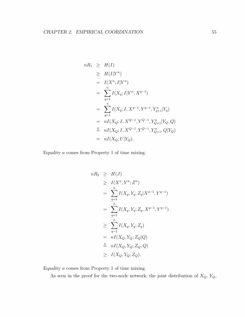
CHAPTER 2. EMPIRICAL COORDINATION 55
nR1 ≥ H(I)
≥ H(I|Y n)
= I(Xn; I|Y n)
=n∑
q=1
I(Xq; I|Y n, Xq−1)
=
n∑
q=1
I(Xq; I, Xq−1, Y q−1, Y nq+1|Yq)
= nI(XQ; I, XQ−1, Y Q−1, Y nQ+1|YQ, Q)
a= nI(XQ; I, XQ−1, Y Q−1, Y n
Q+1, Q|YQ)
= nI(XQ; U |YQ).
Equality a comes from Property 1 of time mixing.
nR2 ≥ H(J)
≥ I(Xn, Y n; Zn)
=n∑
q=1
I(Xq, Yq; Zq|Xq−1, Y q−1)
=
n∑
q=1
I(Xq, Yq; Zq, Xq−1, Y q−1)
≥n∑
q=1
I(Xq, Yq; Zq)
= nI(XQ, YQ; ZQ|Q)
a= nI(XQ, YQ; ZQ, Q)
≥ I(XQ, YQ; ZQ).
Equality a comes from Property 1 of time mixing.
As seen in the proof for the two-node network, the joint distribution of XQ, YQ,
CHAPTER 2. EMPIRICAL COORDINATION 56
and ZQ is arbitrarily close to p0(x, y)p(z|x, y). Therefore, the inequalities of the
coordination capacity region stated in Theorem 8 must hold.
It remains to bound the cardinality of U . We can again use the standard method
of [27]. Notice that p(x, y, z|u) = p(x|u)p(y|x)p(z|y, u) captures all of the Markovity
constraints of the outer bound. Therefore, convex mixtures of distributions of this
form are valid for achieving points in the outer bound. The variable U should have
|X ||Y||Z| − 1 elements to preserve the joint distribution p(x, y, z), which in turn
preserves I(X, Y ; Z) and H(X|Y ), and one more element to preserve H(X|Y, U).
2.4.3 Rate-distortion
We establish the relationship from Theorem 9 between the coordination capacity
region and the rate-distortion region in two parts. First we show that Dp0 contains
ACp0 and then the other way around. To keep clutter to a minimum and without
loss of generality, we only discuss a single distortion measure d, rate R, and a pair of
sequences of actions Xn and Y n.
Coordination implies distortion (Dp0 ⊃ ACp0)
The distortion incurred with respect to a distortion function d on a set of sequences
of actions is a function of the joint type of the sequences. That is,
d(n)(xn, yn) =1
n
n∑
i=1
d(xi, yi)
=1
n
n∑
i=1
∑
x,y
1(xi = x, yi = y)d(x, y)
=∑
x,y
d(x, y)1
n
n∑
i=1
1(xi = x, yi = y)
=∑
x,y
d(x, y)Pxn,yn(x, y)
= EPxn,ynd(X, Y ). (2.13)
When a rate-coordination tuple (R, p(x, y)) is in the interior of the coordination
CHAPTER 2. EMPIRICAL COORDINATION 57
capacity region Cp0, we are assured the existence of a coordination code for any ǫ > 0
for which
Pr(‖PXn,Y n − p‖TV > ǫ) < ǫ.
Therefore, with probability greater that 1 − ǫ,
EPXn,Y n d(X, Y ) ≤ Ep d(X, Y ) + ǫdmax.
Recalling (2.13) yields,
E d(n)(xn, yn) ≤ Ep d(X, Y ) + 2ǫdmax.
As expected, a sequence of (2nR, n) coordination codes that achieves empirical coor-
dination for the joint distribution p(x, y) also achieves the point in the rate-distortion
region with the same rate and with distortion value Ep d(X, Y ).
Distortion implies coordination (Dp0 ⊂ ACp0)
Suppose that a (2nR, n) rate-distortion codes achieves distortion E d(n)(Xn, Y n) ≤ D.
Substituting from (2.13),
E[EPXn,Y nd(X, Y )
]≤ D.
However,
E[EPXn,Y n d(X, Y )
]= EEPXn,Y n d(X, Y )
by linearity.
We can achieve the rate-coordination pair (R,EPXn,Y n) by augmenting the rate-
distortion code. If we repeat the use of the rate-distortion code over k blocks of length
n each, then we induce a joint distribution on (Xkn, Y kn) that consists of i.i.d. sub-
blocks (Xn, Y n), ..., (Xknkn−n+1, Y
knkn−n+1) denoted as (X(1)n, Y (1)n), ..., (X(k)n, Y (k)n).
CHAPTER 2. EMPIRICAL COORDINATION 58
By the weak law of large number,
PXkn,Y kn =1
k
k∑
i=1
PX(i)n,Y (i)n
−→ E PXn,Y n in probability.
Point-wise convergence in probability implies that as k grows
∥∥PXkn,Y kn − E PXn,Y n
∥∥TV
−→ 0 in probability.
Thus, for any point (R, D) in the rate-distortion region we have identified a point
(R,EPXn,Y n) in the coordination capacity region that projects down to it.
Chapter 3
Strong Coordination
3.1 Introduction
Strong coordination addresses questions like this: If two players of a multiplayer
game wish to collaborate, how should they best use communication to generate their
actions?
So far we have examined coordination where the goal is to generate Y n so that the
joint type PXn,Y n(x, y) is equal to p0(x)p(y|x). This goal relates to the joint behavior
at the nodes in the network averaged over time. The order of the (Xi, Yi) pairs doesn’t
matter.
How different does the problem become if we actually want the actions at the
various nodes in the network to be random according to a desired joint distribution?
In this vein, we turn to a stronger notion which we call strong coordination. We
want the induced distribution p(xn, yn) (induced by the coordination code) to be
close to the true target distribution p(xn, yn) =∏n
i=1 p0(xi)p(yi|xi)—so close that a
statistician could not tell the difference, based on (Xn, Y n), of whether (Xn, Y n) ∼ p
or (Xn, Y n) ∼ p. Thus, strong coordination yields an effective simulation of n uses
of the channel p(y|x).
Clearly this new strong coordination objective is more demanding—after all, if
one were to generate random actions, i.i.d. in time, according to the appropriate
joint distribution, then the empirical distribution would also follow suit. However,
59
CHAPTER 3. STRONG COORDINATION 60
in some settings the added feature of coordinating random behavior can be crucial.
For example, in situations where an adversary is involved, it might be important to
maintain a mystery about the actions that will be generated in the network.
Strong coordination has applications in cooperative game theory, reminiscent of
the framework investigated in [8]. Suppose a team shares the same payoff in a re-
peated game setting. An opponent tries to anticipate and exploit patterns in the
team’s combined actions, but a secure line of communication is available to help
them coordinate. Of course, each player could communicate his randomized actions
to the other players, but this is an excessive use of communication. Strong coordina-
tion according to a well-chosen joint distribution will be useful in this situation. This
is explored in Section 3.4.
3.1.1 Problem specifics
Most of the definitions relating to empirical coordination in Chapter 2 carry over to
strong coordination, including the notions of coordination codes and induced distri-
butions. However, in the context of strong coordination, achievability has nothing to
do with the joint type. Here we define strong achievability to mean that the distri-
bution of the time-sequence of actions in the network is close in total variation to the
desired joint distribution, i.i.d. in time. We discuss the strong coordination capacity
region Cp0defined by this notion of strong achievability.
Definition 9 (Strong achievability). A desired distribution p(x, y, z) is strongly achiev-
able if there exists a sequence of (non-deterministic) coordination codes such that the
total variation between the induced distribution p(xn, yn, zn) and the i.i.d. desired
distribution goes to zero. That is,
∥∥∥∥∥p(xn, yn, zn) −n∏
i=1
p(xi, yi, zi)
∥∥∥∥∥TV
−→ 0.
Common randomness plays a crucial role in achieving strong coordination. For
instance, in a network with no communication, only independent actions can be
generated at each node without common randomness, but actions can be generated
CHAPTER 3. STRONG COORDINATION 61
according to any desired joint distribution if enough common randomness is available,
as is illustrated in Figure 1.2 in Chapter 1. In addition, for each desired joint distribu-
tion we can identify a specific bit-rate of common randomness that must be available
to the nodes in the network. This motivates us to deal with common randomness
more precisely.
Aside from the communication in the network, we allow common randomness to
be supplied to each node. However, to quantify the amount of common randomness,
we limit it to a rate of R0 bits per action. For an n-block coordination code, ω is
uniformly distributed on the set Ω = 1, ..., 2nR0. In this way, common randomness
is viewed as a resource alongside communication.
3.1.2 Preliminary observations
The strong coordination capacity region Cp0is not convex in general. This becomes
immediately apparent when we consider a network with no communication and with-
out any common randomness. An arbitrary joint distribution is not strongly achiev-
able without communication or common randomness, but any extreme point in the
probability simplex corresponds to a degenerate distribution that is trivially achiev-
able. Thus we see that convex combinations of achievable points in the strong coordi-
nation capacity region are not necessarily strongly achievable, and cannot be achieved
through simple time-sharing as was done for empirical coordination.
We use total variation as a measurement of fidelity for the distribution of the
actions in the network. This has a number of implications. If two distributions
have a small total variation between them, then a hypothesis test cannot reliably tell
them apart. Additionally, the expected value of a bounded function of these random
variables cannot differ by much. Steinberg and Verdu, for example, also use total
variation as one of a handful of fidelity criteria when considering the simulation of
random variables in [28].
Based on the success of random codebooks in information theory and source coding
in particular, it seems hopeful that we might always be able to use common random-
ness to augment a coordination code intended for empirical coordination to result in
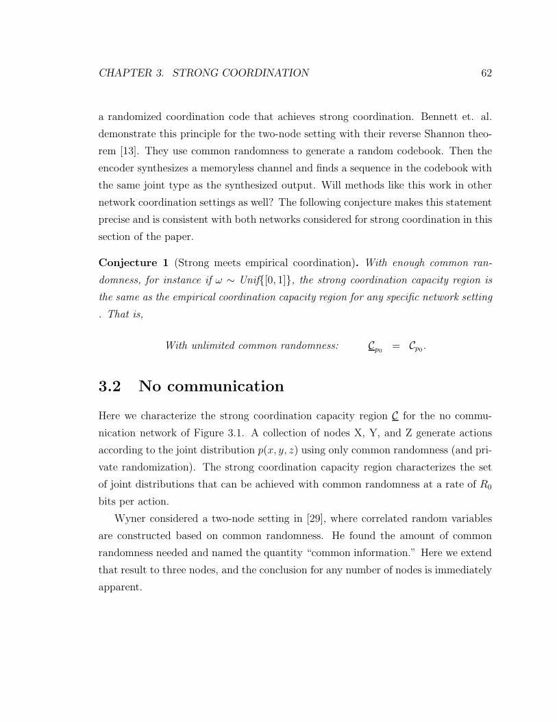
CHAPTER 3. STRONG COORDINATION 62
a randomized coordination code that achieves strong coordination. Bennett et. al.
demonstrate this principle for the two-node setting with their reverse Shannon theo-
rem [13]. They use common randomness to generate a random codebook. Then the
encoder synthesizes a memoryless channel and finds a sequence in the codebook with
the same joint type as the synthesized output. Will methods like this work in other
network coordination settings as well? The following conjecture makes this statement
precise and is consistent with both networks considered for strong coordination in this
section of the paper.
Conjecture 1 (Strong meets empirical coordination). With enough common ran-
domness, for instance if ω ∼ Unif[0, 1], the strong coordination capacity region is
the same as the empirical coordination capacity region for any specific network setting
. That is,
With unlimited common randomness: Cp0= Cp0 .
3.2 No communication
Here we characterize the strong coordination capacity region C for the no commu-
nication network of Figure 3.1. A collection of nodes X, Y, and Z generate actions
according to the joint distribution p(x, y, z) using only common randomness (and pri-
vate randomization). The strong coordination capacity region characterizes the set
of joint distributions that can be achieved with common randomness at a rate of R0
bits per action.
Wyner considered a two-node setting in [29], where correlated random variables
are constructed based on common randomness. He found the amount of common
randomness needed and named the quantity “common information.” Here we extend
that result to three nodes, and the conclusion for any number of nodes is immediately
apparent.
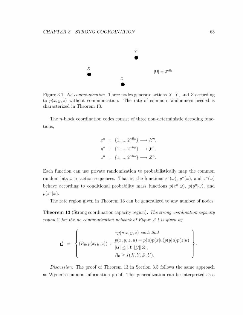
CHAPTER 3. STRONG COORDINATION 63
X
Y
Z
|Ω| = 2nR0
Figure 3.1: No communication. Three nodes generate actions X, Y , and Z accordingto p(x, y, z) without communication. The rate of common randomness needed ischaracterized in Theorem 13.
The n-block coordination codes consist of three non-deterministic decoding func-
tions,
xn : 1, ..., 2nR0 −→ X n,
yn : 1, ..., 2nR0 −→ Yn,
zn : 1, ..., 2nR0 −→ Zn.
Each function can use private randomization to probabilistically map the common
random bits ω to action sequences. That is, the functions xn(ω), yn(ω), and zn(ω)
behave according to conditional probability mass functions p(xn|ω), p(yn|ω), and
p(zn|ω).
The rate region given in Theorem 13 can be generalized to any number of nodes.
Theorem 13 (Strong coordination capacity region). The strong coordination capacity
region C for the no communication network of Figure 3.1 is given by
C =
(R0, p(x, y, z)) :
∃p(u|x, y, z) such that
p(x, y, z, u) = p(u)p(x|u)p(y|u)p(z|u)
|U| ≤ |X ||Y||Z|,R0 ≥ I(X, Y, Z; U).
.
Discussion: The proof of Theorem 13 in Section 3.5 follows the same approach
as Wyner’s common information proof. This generalization can be interpreted as a
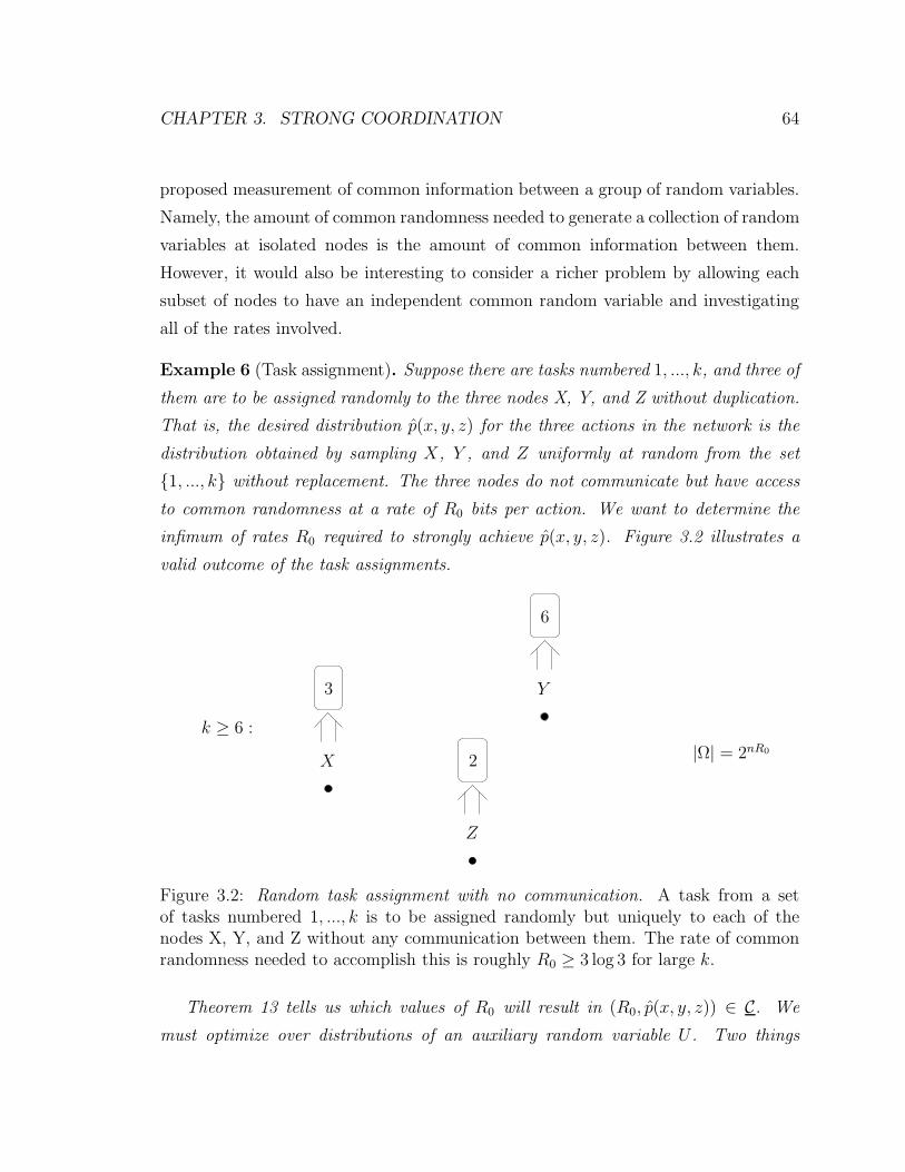
CHAPTER 3. STRONG COORDINATION 64
proposed measurement of common information between a group of random variables.
Namely, the amount of common randomness needed to generate a collection of random
variables at isolated nodes is the amount of common information between them.
However, it would also be interesting to consider a richer problem by allowing each
subset of nodes to have an independent common random variable and investigating
all of the rates involved.
Example 6 (Task assignment). Suppose there are tasks numbered 1, ..., k, and three of
them are to be assigned randomly to the three nodes X, Y, and Z without duplication.
That is, the desired distribution p(x, y, z) for the three actions in the network is the
distribution obtained by sampling X, Y , and Z uniformly at random from the set
1, ..., k without replacement. The three nodes do not communicate but have access
to common randomness at a rate of R0 bits per action. We want to determine the
infimum of rates R0 required to strongly achieve p(x, y, z). Figure 3.2 illustrates a
valid outcome of the task assignments.
X
Z
Y
k ≥ 6 :
3
2
6
|Ω| = 2nR0
Figure 3.2: Random task assignment with no communication. A task from a setof tasks numbered 1, ..., k is to be assigned randomly but uniquely to each of thenodes X, Y, and Z without any communication between them. The rate of commonrandomness needed to accomplish this is roughly R0 ≥ 3 log 3 for large k.
Theorem 13 tells us which values of R0 will result in (R0, p(x, y, z)) ∈ C. We
must optimize over distributions of an auxiliary random variable U . Two things
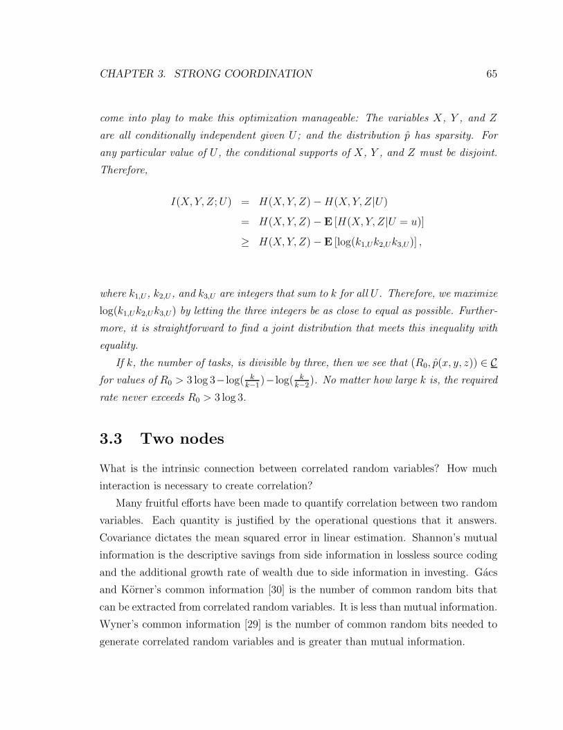
CHAPTER 3. STRONG COORDINATION 65
come into play to make this optimization manageable: The variables X, Y , and Z
are all conditionally independent given U ; and the distribution p has sparsity. For
any particular value of U , the conditional supports of X, Y , and Z must be disjoint.
Therefore,
I(X, Y, Z; U) = H(X, Y, Z) − H(X, Y, Z|U)
= H(X, Y, Z) −E [H(X, Y, Z|U = u)]
≥ H(X, Y, Z) −E [log(k1,Uk2,Uk3,U)] ,
where k1,U , k2,U , and k3,U are integers that sum to k for all U . Therefore, we maximize
log(k1,Uk2,Uk3,U) by letting the three integers be as close to equal as possible. Further-
more, it is straightforward to find a joint distribution that meets this inequality with
equality.
If k, the number of tasks, is divisible by three, then we see that (R0, p(x, y, z)) ∈ Cfor values of R0 > 3 log 3− log( k
k−1)− log( k
k−2). No matter how large k is, the required
rate never exceeds R0 > 3 log 3.
3.3 Two nodes
What is the intrinsic connection between correlated random variables? How much
interaction is necessary to create correlation?
Many fruitful efforts have been made to quantify correlation between two random
variables. Each quantity is justified by the operational questions that it answers.
Covariance dictates the mean squared error in linear estimation. Shannon’s mutual
information is the descriptive savings from side information in lossless source coding
and the additional growth rate of wealth due to side information in investing. Gacs
and Korner’s common information [30] is the number of common random bits that
can be extracted from correlated random variables. It is less than mutual information.
Wyner’s common information [29] is the number of common random bits needed to
generate correlated random variables and is greater than mutual information.
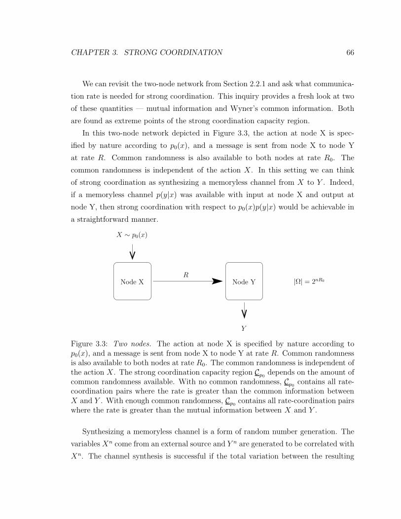
CHAPTER 3. STRONG COORDINATION 66
We can revisit the two-node network from Section 2.2.1 and ask what communica-
tion rate is needed for strong coordination. This inquiry provides a fresh look at two
of these quantities — mutual information and Wyner’s common information. Both
are found as extreme points of the strong coordination capacity region.
In this two-node network depicted in Figure 3.3, the action at node X is spec-
ified by nature according to p0(x), and a message is sent from node X to node Y
at rate R. Common randomness is also available to both nodes at rate R0. The
common randomness is independent of the action X. In this setting we can think
of strong coordination as synthesizing a memoryless channel from X to Y . Indeed,
if a memoryless channel p(y|x) was available with input at node X and output at
node Y, then strong coordination with respect to p0(x)p(y|x) would be achievable in
a straightforward manner.
X ∼ p0(x)
Y
RNode X Node Y |Ω| = 2nR0
Figure 3.3: Two nodes. The action at node X is specified by nature according top0(x), and a message is sent from node X to node Y at rate R. Common randomnessis also available to both nodes at rate R0. The common randomness is independent ofthe action X. The strong coordination capacity region Cp0
depends on the amount ofcommon randomness available. With no common randomness, Cp0
contains all rate-coordination pairs where the rate is greater than the common information betweenX and Y . With enough common randomness, Cp0
contains all rate-coordination pairswhere the rate is greater than the mutual information between X and Y .
Synthesizing a memoryless channel is a form of random number generation. The
variables Xn come from an external source and Y n are generated to be correlated with
Xn. The channel synthesis is successful if the total variation between the resulting
CHAPTER 3. STRONG COORDINATION 67
distribution of (Xn, Y n) and the i.i.d. distribution that would result from passing Xn
through a memoryless channel is small. This total variation requirement means that
any hypothesis test that a statistician comes up with to determine whether Xn was
passed through a real memoryless channel or the channel synthesizer will be virtually
useless.
Wyner’s result implies that in order to generate Xn and Y n separately as an i.i.d.
source pair they must share bits at a rate of at least the common information C(X; Y )
of the joint distribution.1 In the two-node network of Figure 3.3, the description of
Xn at rate R serves the role of shared bits. However, the “reverse Shannon theorem”
of Bennett et. al. [13] suggests that a description rate R > I(X; Y ) is all that is
needed to successfully synthesize a channel. Does this entail a contradiction?
The resolution of Wyner’s work and the work of Bennett et. al. is in the common
randomness. Even though the common randomness at rate R0 is independent of the
action sequence Xn, it still assists in establishing a connection between the action se-
quences Xn and Y n and opens the way for description rates smaller than the common
information C(X; Y ).
We give the full characterization of the strong coordination capacity region Cp0for
this two-node network2, involving a tradeoff between the description rate R and the
rate of common randomness R0, which indeed confirms the two extreme cases: If the
encoder and decoder are provided with enough common randomness, sending I(X; Y )
bits per action suffices. On the other hand, in the absence of common randomness
one must spend C(X; Y ) bits per action.
The (2nR, n) coordination codes consist of a non-deterministic encoding function,
i : X n × 1, ..., 2nR0 −→ 1, ..., 2nR.
and a non-deterministic decoding function,
yn : 1, ..., 2nR × 1, ..., 2nR0 −→ Yn.
1To achieve strong coordination with a rate as low as the common information one must changeWyner’s relative entropy requirement in [29] to a total variation requirement as used in this work.
2This result was independently discovered by Bennett et. al. [31].
CHAPTER 3. STRONG COORDINATION 68
Both functions can use private randomization to probabilistically map the arguments
onto the range of the function. That is, the encoding function i(xn, ω) behaves accord-
ing to a conditional probability mass function p(i|xn, ω), and the decoding function
yn(i, ω) behaves according to a conditional probability mass function p(yn|i, ω).
The actions Xn are chosen by nature i.i.d. according to p0(x), and the actions Y n
are constructed by implementing the non-deterministic coordination code as
Y n = yn(i(Xn, ω), ω).
Let us define two quantities before stating the result. The first is Wyner’s common
information C(X; Y ) [29], which turns out to be the communication rate requirement
for strong coordination in the two-node network when no common randomness is
available:
C(X; Y ) , minU : X−U−Y
I(X, Y ; U),
where the notation X − U − Y represents a Markov chain from X to U to Y . The
second quantity we call necessary conditional entropy H(Y †X), which we will show to
be the amount of common randomness needed to maximize the strong coordination
capacity region in the two-node network:
H(Y †X) , minf : X−f(Y )−Y
H(f(Y )|X).
Theorem 14 (Strong coordination capacity region). The strong coordination capacity
region Cp0for the two-node network of Figure 3.3 is given by
Cp0=
(R0, R, p(y|x)) :
∃p(u|x, y) such that
|U| ≤ |X ||Y| + 1,
R ≥ I(X; U),
R0 + R ≥ I(X, Y ; U).
.
Furthermore, the rate pair (R0, I(X; Y )) is in the strong rate-coordination region Rp0
CHAPTER 3. STRONG COORDINATION 69
if and only if the rate of common randomness R0 ≥ H(Y †X).
3.3.1 Insights
Two extreme points of the strong coordination capacity region Cp0are manifested
directly in the inequalities of Theorem 14. If R0 = 0, the second inequality dominates.
Thus, the minimum communication rate R is Wyner’s common information C(X; Y ).
At the other extreme, using the data processing inequality on the first inequality
yields R ≥ I(X; Y ) no matter how much common randomness is available, and this
is achieved when R0 ≥ H(Y †X). We show in Section 3.5 that in fact H(Y †X) is
the minimum rate of common randomness for which R = I(X; Y ) is in the strong
rate-coordination region Rp0. For many joint distributions, the necessary conditional
entropy H(Y †X) will simply equal the conditional entropy H(Y |X).
This theorem is consistent with Conjecture 1—with enough common randomness,
the strong coordination capacity region Cp0is the same as the coordination capacity
region Cp0 found in Section 2.2.1.
The proof of Theorem 14 is found in Section 3.5.
Example 7 (Task assignment). Consider again a task assignment setting similar to
Example 6, where tasks are numbered 1, ..., k and are to be assigned randomly to the
two nodes X and Y without duplication. The action X is supplied by nature, uni-
formly at random, and the desired distribution p(y|x) for the action Y is the uniform
distribution over all tasks not equal to X. Figure 3.4 illustrates a valid outcome of
the task assignments.
To apply Theorem 14 we must evaluate the three quantities I(X; Y ), C(X; Y ),
and H(Y †X). For the joint distribution p0(x)p(y|x), the necessary conditional entropy
H(Y †X) is exactly the conditional entropy H(Y |X). The computation of the common
information C(X; Y ) follows the same steps as the derivation found in Example 6.
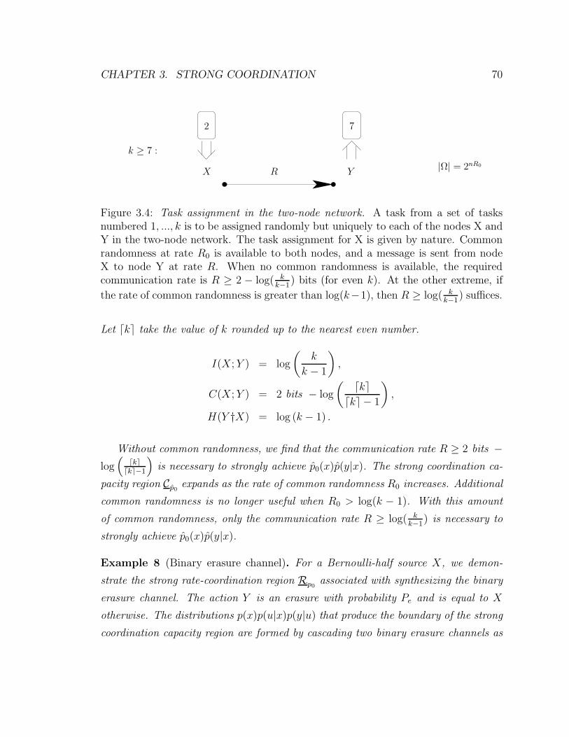
CHAPTER 3. STRONG COORDINATION 70
X YR
k ≥ 7 :
2 7
|Ω| = 2nR0
Figure 3.4: Task assignment in the two-node network. A task from a set of tasksnumbered 1, ..., k is to be assigned randomly but uniquely to each of the nodes X andY in the two-node network. The task assignment for X is given by nature. Commonrandomness at rate R0 is available to both nodes, and a message is sent from nodeX to node Y at rate R. When no common randomness is available, the requiredcommunication rate is R ≥ 2 − log( k
k−1) bits (for even k). At the other extreme, if
the rate of common randomness is greater than log(k−1), then R ≥ log( kk−1
) suffices.
Let ⌈k⌉ take the value of k rounded up to the nearest even number.
I(X; Y ) = log
(k
k − 1
),
C(X; Y ) = 2 bits − log
( ⌈k⌉⌈k⌉ − 1
),
H(Y †X) = log (k − 1) .
Without common randomness, we find that the communication rate R ≥ 2 bits −log(
⌈k⌉⌈k⌉−1
)is necessary to strongly achieve p0(x)p(y|x). The strong coordination ca-
pacity region C p0expands as the rate of common randomness R0 increases. Additional
common randomness is no longer useful when R0 > log(k − 1). With this amount
of common randomness, only the communication rate R ≥ log( kk−1
) is necessary to
strongly achieve p0(x)p(y|x).
Example 8 (Binary erasure channel). For a Bernoulli-half source X, we demon-
strate the strong rate-coordination region Rp0associated with synthesizing the binary
erasure channel. The action Y is an erasure with probability Pe and is equal to X
otherwise. The distributions p(x)p(u|x)p(y|u) that produce the boundary of the strong
coordination capacity region are formed by cascading two binary erasure channels as
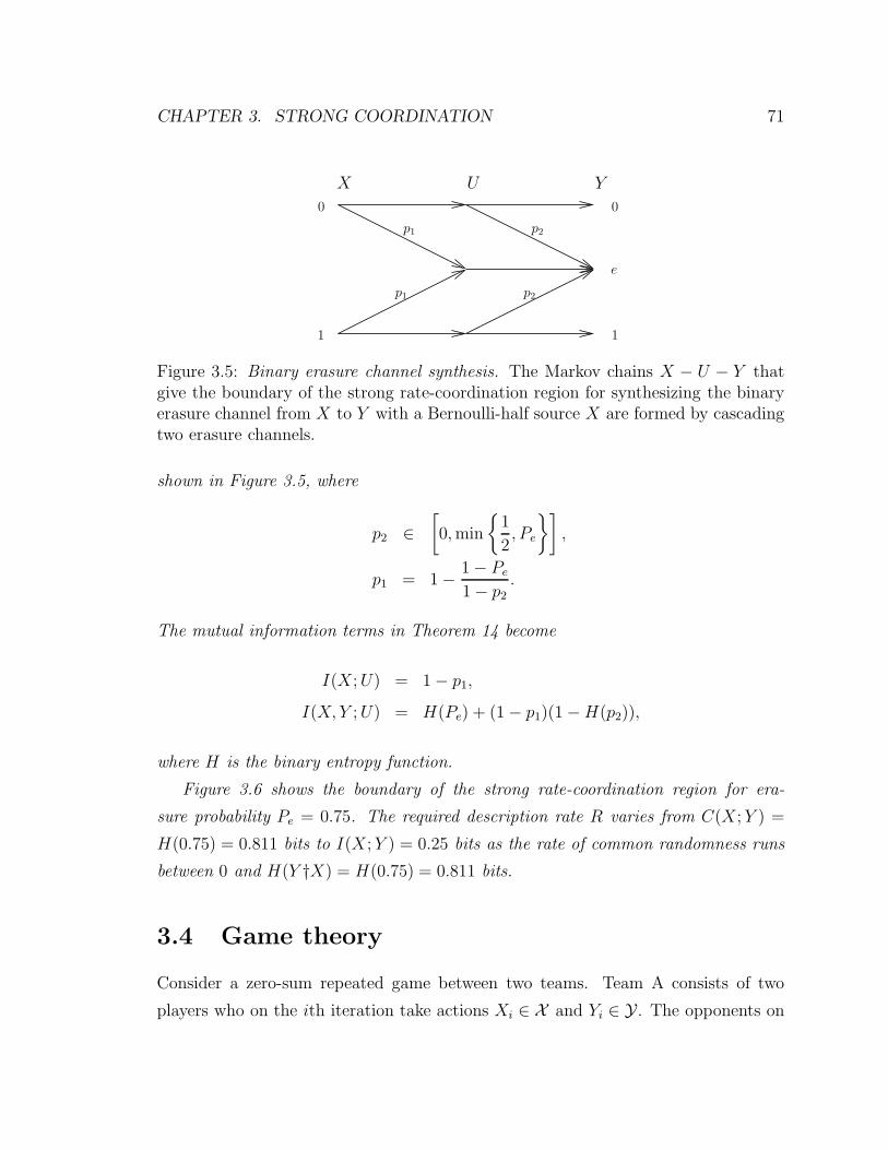
CHAPTER 3. STRONG COORDINATION 71
X U Y
0
1
p1
p1
p2
p2
0
e
1
Figure 3.5: Binary erasure channel synthesis. The Markov chains X − U − Y thatgive the boundary of the strong rate-coordination region for synthesizing the binaryerasure channel from X to Y with a Bernoulli-half source X are formed by cascadingtwo erasure channels.
shown in Figure 3.5, where
p2 ∈[0, min
1
2, Pe
],
p1 = 1 − 1 − Pe
1 − p2
.
The mutual information terms in Theorem 14 become
I(X; U) = 1 − p1,
I(X, Y ; U) = H(Pe) + (1 − p1)(1 − H(p2)),
where H is the binary entropy function.
Figure 3.6 shows the boundary of the strong rate-coordination region for era-
sure probability Pe = 0.75. The required description rate R varies from C(X; Y ) =
H(0.75) = 0.811 bits to I(X; Y ) = 0.25 bits as the rate of common randomness runs
between 0 and H(Y †X) = H(0.75) = 0.811 bits.
3.4 Game theory
Consider a zero-sum repeated game between two teams. Team A consists of two
players who on the ith iteration take actions Xi ∈ X and Yi ∈ Y . The opponents on
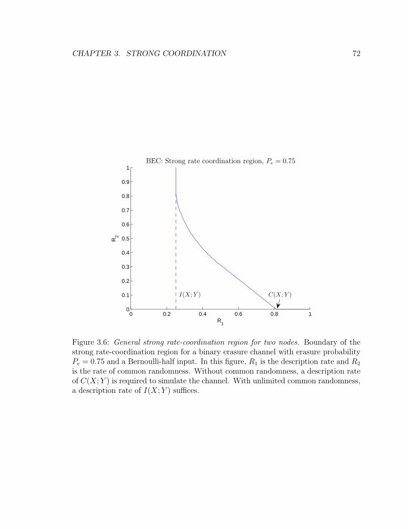
CHAPTER 3. STRONG COORDINATION 72
0 0.2 0.4 0.6 0.8 10
0.1
0.2
0.3
0.4
0.5
0.6
0.7
0.8
0.9
1
R1
R2
BEC: Strong rate coordination region, Pe = 0.75
I(X; Y ) C(X; Y )
Figure 3.6: General strong rate-coordination region for two nodes. Boundary of thestrong rate-coordination region for a binary erasure channel with erasure probabilityPe = 0.75 and a Bernoulli-half input. In this figure, R1 is the description rate and R2
is the rate of common randomness. Without common randomness, a description rateof C(X; Y ) is required to simulate the channel. With unlimited common randomness,a description rate of I(X; Y ) suffices.
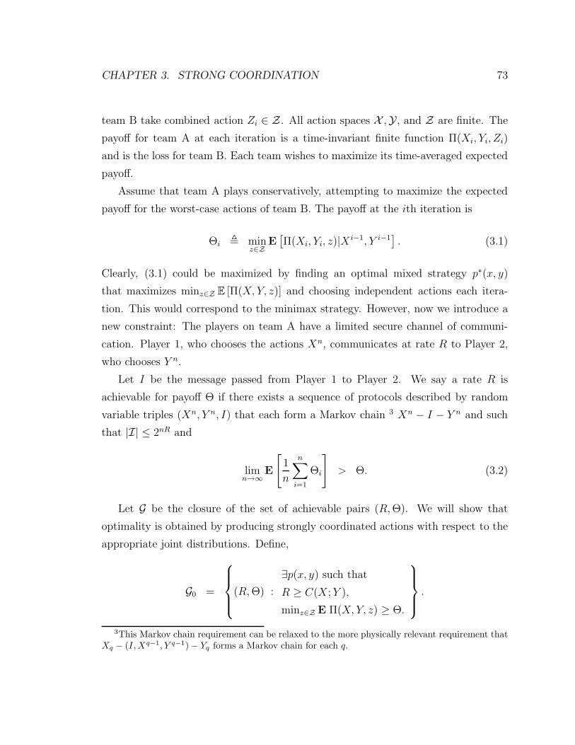
CHAPTER 3. STRONG COORDINATION 73
team B take combined action Zi ∈ Z. All action spaces X ,Y, and Z are finite. The
payoff for team A at each iteration is a time-invariant finite function Π(Xi, Yi, Zi)
and is the loss for team B. Each team wishes to maximize its time-averaged expected
payoff.
Assume that team A plays conservatively, attempting to maximize the expected
payoff for the worst-case actions of team B. The payoff at the ith iteration is
Θi , minz∈Z
E[Π(Xi, Yi, z)|X i−1, Y i−1
]. (3.1)
Clearly, (3.1) could be maximized by finding an optimal mixed strategy p∗(x, y)
that maximizes minz∈Z E [Π(X, Y, z)] and choosing independent actions each itera-
tion. This would correspond to the minimax strategy. However, now we introduce a
new constraint: The players on team A have a limited secure channel of communi-
cation. Player 1, who chooses the actions Xn, communicates at rate R to Player 2,
who chooses Y n.
Let I be the message passed from Player 1 to Player 2. We say a rate R is
achievable for payoff Θ if there exists a sequence of protocols described by random
variable triples (Xn, Y n, I) that each form a Markov chain 3 Xn − I − Y n and such
that |I| ≤ 2nR and
limn→∞
E
[1
n
n∑
i=1
Θi
]> Θ. (3.2)
Let G be the closure of the set of achievable pairs (R, Θ). We will show that
optimality is obtained by producing strongly coordinated actions with respect to the
appropriate joint distributions. Define,
G0 =
(R, Θ) :
∃p(x, y) such that
R ≥ C(X; Y ),
minz∈Z E Π(X, Y, z) ≥ Θ.
.
3This Markov chain requirement can be relaxed to the more physically relevant requirement thatXq − (I, Xq−1, Y q−1) − Yq forms a Markov chain for each q.
CHAPTER 3. STRONG COORDINATION 74
Theorem 15 (Optimal cooperative play).
G = ConvexHull(G0).
3.5 Proofs
Properties of total variation
Here we list a number of properties of total variation that are useful resources for
both the achievability and converse proofs of this chapter.
Lemma 16 (Total variation: marginal). For any two joint distributions p(a, b) and
p(a, b) on the same probability space, the total variation distance between them can
only be reduced when attention is restricted to marginal distributions p(a) and p(a).
That is,
‖p(a) − p(a)‖TV ≤ ‖p(a, b) − p(a, b)‖TV .
Proof.
‖p(a) − p(a)‖TV =∑
a
|p(a) − p(a)|
=∑
a
∣∣∣∣∣∑
b
p(a, b) −∑
b
p(a, b)
∣∣∣∣∣
≤∑
a
∑
b
|p(a, b) − p(a, b)|
= ‖p(a, b) − p(a, b)‖TV .
Lemma 17 (Total variation: same channel). When two random variables are passed
through the same channel, the total variation between the resulting input-output joint
CHAPTER 3. STRONG COORDINATION 75
distributions is the same as the total variation between the input distributions. Specif-
ically,
‖p(a) − p(a)‖TV = ‖p(a)p(b|a) − p(a)p(b|a)‖TV .
Proof.
‖p(a) − p(a)‖TV =∑
a
|p(a) − p(a)|
=∑
a
(∑
b
p(b|a)
)|p(a) − p(a)|
=∑
a
∑
b
|p(b|a)(p(a) − p(a))|
=∑
a
∑
b
|p(a)p(b|a) − p(a)p(b|a)|
= ‖p(a)p(b|a) − p(a)p(b|a)‖TV .
Let Q ∈ 1, ..., n be a random time index, independent of the random sequence
Xn, and let the variable XQ be defined along the lines of time mixing in Section 2.4.2.
Lemma 18 (Total variation: random time). The total variation between the distri-
butions of two random sequences is an upper bound on the total variation between the
distributions of the variables in the sequence at a random time index. That is,
‖pXQ(x) − pXQ
(x)‖TV ≤ ‖p(xn) − p(xn)‖TV .
CHAPTER 3. STRONG COORDINATION 76
Proof.
‖pXQ(x) − pXQ
(x)‖TV =
∥∥∥∥∥∑
q
p(q)(pXq(x) − pXq(x))
∥∥∥∥∥TV
≤∑
x,q
p(q)|pXq(x) − pXq(x)|
=∑
q
p(q)‖pXq(x) − pXq(x)‖TV
a≤
∑
q
p(q)‖p(xn) − p(xn)‖TV
= ‖p(xn) − p(xn)‖TV ,
where inequality a comes from applying Lemma 16.
3.5.1 Achievability
The following phenomenon was noticed both by Wyner [29] and by Han and Verdu
[12]. Consider a memoryless channel p(v|u). A channel input with distribution p(u)
induces an output with distribution p(v) =∑
u p(u)p(v|u). If the inputs are i.i.d. then
the outputs are i.i.d. as well. Now suppose that instead a channel input sequence
Un is chosen uniformly at random from a set C of 2nR deterministic sequences. If
R > I(U ; V ) then the set C can be chosen so that the output distribution is arbitrarily
close in total variation to the i.i.d. distribution∏n
i=1 p(vi) for large enough n. This
is the claim made by Lemma 19, and we provide our own simple proof.
Cloud mixing
We adopt the use of jointly typical sets T (n)ǫ from Section 2.4.
Consider a memoryless channel from U to V defined by the conditional probability
distribution p(v|u). For an input distribution p(u), we say that the desired output
distribution is i.i.d. with respect to the distribution induced by the channel p(v) =
CHAPTER 3. STRONG COORDINATION 77
∑u p(u)p(v|u). That is,
p(vn) =n∏
i=1
p(vi)
=
n∏
i=1
∑
u
p(u)p(vi|u).
Consider an input codebook C of 2nR sequences un(1), ..., un(2nR), each constructed
randomly and independently according to the i.i.d. input distribution Un(i) ∼∏n
i=1 p(ui). Also, let M be a random selection of one of the sequences un(M) in
the codebook C, uniformly at random.
The combination of selecting a random sequence from the input codebook C and
using it as the input to the memoryless channel p(v|u) results in an induced output
distribution,
P (vn) = 2−nR∑
m
p(vn|Un(m)).
where p(vn|un) =∏n
i=1 p(vi|ui). We use capital letters P and Un(m) to indicate that
they are random due to the random generation of the input codebook C. Therefore,
P (vn) is a random probability mass function on vn sequences that depends on the
particular codebook. The intention of Lemma 19 is to show that if R is large enough,
P (vn) will be close in total variation to p(vn) for most codebooks.
Lemma 19 (Cloud mixing). For a memoryless channel defined by p(v|u), an input
distribution p(u), and an input codebook of size 2nR, the total variation distance be-
tween the induced output distribution and the desired output distribution goes to zero
as n goes to infinity if R > I(U ; V ). That is,
R > I(U ; V ) =⇒ limn→∞
E∥∥∥P (vn) − p(vn)
∥∥∥TV
= 0.
Proof. We need to separate the jointly typical sequences from the rest. We start by
CHAPTER 3. STRONG COORDINATION 78
separating P (vn) into two parts,
P1(vn) , 2−nR
∑
m
p(vn|Un(m))1((Un(m), vn) ∈ T (n)
ǫ
),
P2(vn) , 2−nR
∑
m
p(vn|Un(m))1((Un(m), vn) /∈ T (n)
ǫ
).
Notice a couple of observations. First, P (vn) = P1(vn) + P2(v
n). Second, the
expected value of P (vn) with respect to the randomly generated input codebook is
the desired distribution p(vn). That is,
E P (vn)a= 2−nR
∑
m
E p(vn|Un(m))
b= E p(vn|Un(1))
=∑
un
n∏
i=1
p(ui)n∏
j=1
p(vj |uj)
= p(vn),
where equality a is an application of the linearity of expectation to the definition of
P (vn), and equality b is due to the i.i.d. nature of the input codebook C.
CHAPTER 3. STRONG COORDINATION 79
We separate the total variation distance E∣∣∣∣∣∣P (vn) − p(vn)
∣∣∣∣∣∣TV
into three parts:
E∥∥∥P (vn) − p(vn)
∥∥∥TV
= E∥∥∥P (vn) − E P (vn)
∥∥∥TV
=∑
vn
E∣∣∣P (vn) − E P (vn)
∣∣∣
=∑
vn∈T (n)ǫ
E∣∣∣P (vn) − E P (vn)
∣∣∣
+∑
vn /∈T (n)ǫ
E∣∣∣P (vn) −E P (vn)
∣∣∣
a≤
∑
vn∈T (n)ǫ
E∣∣∣P1(v
n) − E P1(vn)∣∣∣
+∑
vn
E∣∣∣P2(v
n) −E P2(vn)∣∣∣
+∑
vn /∈T (n)ǫ
E∣∣∣P (vn) −E P (vn)
∣∣∣ , (3.3)
where inequality a is due to the triangle inequality and adding more terms into the
second sum.
The first sum in (3.3) is the interesting one to consider, so we save it for last. Both
other sums are resolved by the A.E.P. For instance, the triangle inequality gives us,
∑
vn
E∣∣∣P2(v
n) − E P2(vn)∣∣∣ ≤ 2
∑
vn
E P2(vn)
= 2∑
vn
2−nR∑
m
E p(vn|Un(m))1((Un(m), vn) /∈ T (n)
ǫ
)
= 2∑
vn
E p(vn|Un(1))1((Un(1), vn) /∈ T (n)
ǫ
)
= 2∑
(un,vn)/∈T (n)ǫ
p(un)p(vn|un)
= 2(1 − Pr
(T (n)
ǫ
))
→ 0 as n goes to infinity,
CHAPTER 3. STRONG COORDINATION 80
and
∑
vn /∈T (n)ǫ
E∣∣∣P (vn) − E P (vn)
∣∣∣ ≤ 2∑
vn /∈T (n)ǫ
E P (vn)
= 2∑
vn /∈T (n)ǫ
p(vn)
→ 0 as n goes to infinity.
The remaining term in (3.3) deals with only jointly typical sequences. We derive a
uniform bound for all typical sequences vn ∈ T (n)ǫ , starting with the Jensen inequality,
E∣∣∣P1(v
n) − E P1(vn)∣∣∣ ≤
√E(P1(vn) − E P1(vn)
)2
=
√Var P1(vn)
Since the input codebook C is a collection of sequences generated i.i.d., the variance
of P1(vn) breaks down nicely as
Var P1(vn)
a= 2−nRVar
(p(vn|Un(1))1
((Un(1), vn) ∈ T (n)
ǫ
))
≤ 2−nRE(p(vn|Un(1))1
((Un(1), vn) ∈ T (n)
ǫ
))2
= 2−nR∑
un : (un,vn)∈T (n)ǫ
p(un)p2(vn|un)
b≤ 2−n(R+H(V |U)−δ1(ǫ))
∑
un
p(un)p(vn|un)
= 2−n(R+H(V |U)−δ1(ǫ))p(vn)
≤ 2−n(R+H(V |U)+H(V )−δ2(ǫ)) for all typical vn sequences,
where δ1(ǫ)) and δ2(ǫ)) go to zero as ǫ goes to zero. Equality a comes from the
definition of P1(vn), and inequality b is a result of continuity of the entropy function
and the fact that un and vn are ǫ-jointly typical.
CHAPTER 3. STRONG COORDINATION 81
The conclusion with respect to the first term in (3.3) is,
∑
vn∈T (n)ǫ
E∣∣∣P1(v
n) − E P1(vn)∣∣∣ ≤
∑
vn∈T (n)ǫ
2−n2(R+H(V |U)+H(V )−δ2(ǫ))
≤ 2−n2(R+H(V |U)−H(V )−δ3(ǫ))
= 2−n2(R−I(U ;V )−δ3(ǫ)),
where δ3(ǫ)) goes to zero as ǫ goes to zero. Clearly, if R > I(U ; V ) then a small
enough choice of ǫ exists to make this term converge to zero as n goes to infinity.
No communication - Theorem 13
The network of Figure 3.1 with no communication generalizes Wyner’s common in-
formation work [29] to three nodes. Figure 3.7 illustrates how to achieve the strong
coordination capacity region C of Theorem 13. Let each decoder simulate a memory-
less channel from U to X, Y , or Z, depending on the particular node. The common
randomness ω is used to index a sequence Un(ω) that is used as the inputs to the
channels.
Notice that the action sequences Xn, Y n, and Zn produced via these three separate
channels are distributed the same as if they were generated as outputs of a single
channel because p(x, y, z|u) = p(x|u)p(y|u)p(z|u) according to the definition of C in
Theorem 13. Since R > I(X, Y, Z; U) for points in the interior of C, Lemma 19
confirms that this scheme will achieve strong coordination.
Two nodes - Theorem 14 - region
Strong coordination is achieved in the two-node network of Figure 3.3 in much the
same way as in the no-communication network. One key difference, however, is that
the action X is given randomly by nature in the two-node network.
We construct efficient coordination codes for the two-node network in a round-
about way. For analysis purposes, assume that we are allowed to generate the se-
quences Xn at node X as well as Y n at node Y based on shared messages. The
index I and the index J are both available to both nodes. We will derive legitimate
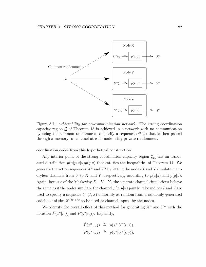
CHAPTER 3. STRONG COORDINATION 82
ω
Common randomness
Node X
Node Y
Node Z
p(x|u)
p(y|u)
p(z|u)
Un(ω)
Un(ω)
Un(ω)
Xn
Y n
Zn
Figure 3.7: Achievability for no-communication network. The strong coordinationcapacity region C of Theorem 13 is achieved in a network with no communicationby using the common randomness to specify a sequence Un(ω) that is then passedthrough a memoryless channel at each node using private randomness.
coordination codes from this hypothetical construction.
Any interior point of the strong coordination capacity region Cp0has an associ-
ated distribution p(u)p(x|u)p(y|u) that satisfies the inequalities of Theorem 14. We
generate the action sequences Xn and Y n by letting the nodes X and Y simulate mem-
oryless channels from U to X and Y , respectively, according to p(x|u) and p(y|u).
Again, because of the Markovity X −U −Y , the separate channel simulations behave
the same as if the nodes simulate the channel p(x, y|u) jointly. The indices I and J are
used to specify a sequence Un(I, J) uniformly at random from a randomly generated
codebook of size 2n(R0+R) to be used as channel inputs by the nodes.
We identify the overall effect of this method for generating Xn and Y n with the
notation P (xn|i, j) and P (yn|i, j). Explicitly,
P (xn|i, j) , p(xn|Un(i, j)),
P (yn|i, j) , p(yn|Un(i, j)).
CHAPTER 3. STRONG COORDINATION 83
These conditional distributions are random because the input codebook of Un(i, j)
sequences is randomly generated. Furthermore, we define the backward induced joint
distribution
P (xn, yn, i, j) , 2−n(R0+R)P (xn|i, j)P (yn|i, j),
from which marginal and conditional distributions can be derived.
Lemma 19 allows us to draw two conclusions about this backward induced joint
distribution. The fact that R0 + R > I(X, Y ; U) tells us,
limn→∞
E∥∥∥P (xn, yn) − p(xn, yn)
∥∥∥TV
= 0,
and R > I(X; U) gives,
limn→∞
E∥∥∥P (xn, j) − p(xn)p(j)
∥∥∥TV
= limn→∞
∑
j
p(j)∑
xn
E∣∣∣P (xn|j) − p(xn)
∣∣∣
= limn→∞
E∥∥∥P (xn|j = 1) − p(xn)
∥∥∥TV
= 0.
The idea is that R is large enough so that J is roughly independent of Xn. For
any particular value of J , there are enough sequences in the codebook due to the
varying index I that the dependence between Xn and J is washed away.
Finally, we specify the coordination codes for each n for the two-node network
by the conditional distributions derived from the backward induced joint distribution
P (xn, yn, i, j). Given an input codebook C, the encoder implements P (i|xn, j) where
it is well defined and otherwise sends the index 1. The decoder implements P (yn|i, j).Using these coordination codes, a new induced distribution P will result. This
distribution is given by
P (xn, yn, i, j) = p(xn)p(j)P (i|xn, j)P (yn|i, j).
CHAPTER 3. STRONG COORDINATION 84
The induced joint distribution P (xn, yn, i, j) and the backward induced joint distri-
bution P (xn, yn, i, j) are both comprised of differing joint distributions on Xn and J
passed through the same channel P (i|xn, j)P (yn|i, j).We conclude,
∥∥∥P (xn, yn) − p(xn, yn)∥∥∥
TV
a
≤∥∥∥P (xn, yn) − P (xn, yn)
∥∥∥TV
+∥∥∥P (xn, yn) − p(xn, yn)
∥∥∥TV
b≤
∥∥∥P (xn, yn, i, j) − P (xn, yn, i, j)∥∥∥
TV
+∥∥∥P (xn, yn) − p(xn, yn)
∥∥∥TV
c=
∥∥∥p(xn)p(j) − P (xn, j)∥∥∥
TV
+∥∥∥P (xn, yn) − p(xn, yn)
∥∥∥TV
,
where a comes from the triangle inequality, b is an application of Lemma 16, and c is
a consequence of Lemma 17. The result is,
limn→∞
E∥∥∥P (xn, yn) − p(xn, yn)
∥∥∥TV
= 0,
so there exists a sequence of codebooks that sends total variation to zero as n grows.
Two nodes - Theorem 14 - extreme point
In addition to characterizing the strong coordination capacity region for the two-
node network, Theorem 14 states that (R0, I(X; Y )) is in the strong rate-coordination
region Rp0if R0 ≥ H(Y †X). This is a straightforward application of the definition
of H(Y †X). We can verify this with the following choice of U :
U = argminf(Y ) : X−f(Y )−Y
H(f(Y )|X).
Notice that this choice of U separates X and Y into a Markov chain by definition.
Also, the mutual information I(X; U) is less than or equal to I(X; Y ), since U is
CHAPTER 3. STRONG COORDINATION 85
a function of Y , thus satisfying the first rate inequality in Cp0as characterized by
Theorem 14. The second inequality is satisfied because of the chain rule,
I(X, Y ; U) = I(X; U) + I(Y ; U |X)
= I(X; U) + H(Y †X)
≤ I(X; Y ) + H(Y †X).
Comments
The efficient coordination codes presented in Section 3.5.1 have some resemblance
to classical source coding in the rate-distortion sense. The difference here is that
sequences in the codebook do not correspond to reconstruction sequences. Instead,
randomization happens at both ends, both at the encoder via common randomness
and at the decoder via private randomization.
3.5.2 Converse
Mutual information bounds for nearly i.i.d. sequences
If two finite-alphabet random variables have distributions that are close in total vari-
ation, then their entropies are also close (Theorem 16.3.2 of [26]). This leads to a
couple of lemmas concerning a sequence of random variables W n with a distribution
that is close to an i.i.d. distribution. First, the total mutual information with the past∑n
q=1 I(Wq; Wq−1) is small. Second, the mutual information between an independent
random time index Q and the variable at that time index WQ is small.
Lemma 20 (Information with the past). For any discrete random sequence W n ∈Wn, if there exists a distribution p(w) on the alphabet W such that
∥∥∥∥∥p(wn) −n∏
q=1
p(wq)
∥∥∥∥∥TV
< ǫ < 1/2,
CHAPTER 3. STRONG COORDINATION 86
then the total mutual information with the past∑n
q=1 I(Wq; Wq−1) is bounded by
n∑
q=1
I(Wq; Wq−1) ≤ 2nǫ
(log |W| + log
1
ǫ
).
Proof. First use Lemma 16 to claim that every symbol in W n must be close in dis-
tribution to p. That is,
∥∥pWq(w) − p(w)∥∥
TV< ǫ for all q ∈ 1, ..., n.
Let W n be distributed according to∏n
q=1 p(wq). Then by Theorem 17.3.3 of [26],
∣∣∣H(W n) − H(W n)∣∣∣ ≤ ǫ log
( |W|nǫ
), (3.4)
∣∣∣H(Wq) − H(Wq)∣∣∣ ≤ ǫ log
( |W|ǫ
)for all q ∈ 1, ..., n. (3.5)
Because W n is an i.i.d. sequence, H(W n) =∑n
k=1 H(Wk). Therefore,
n∑
q=1
I(Wq; Wq−1) =
n∑
q=1
H(Wq) − H(W n)
=n∑
q=1
(H(Wq) − H(Wq)
)+ H(W n) − H(W n)
≤ nǫ log
( |W|ǫ
)+ ǫ log
( |W|nǫ
)
= 2nǫ log |W| + (n + 1)ǫ log1
ǫ
≤ 2nǫ
(log |W| + log
1
ǫ
).
Lemma 21 (Timing information). For any discrete random sequence W n ∈ Wn, if
CHAPTER 3. STRONG COORDINATION 87
there exists a distribution p(w) on the alphabet W such that
∥∥∥∥∥p(wn) −n∏
q=1
p(wq)
∥∥∥∥∥TV
< ǫ < 1/2,
then for a random time variable Q ∈ 1, ..., n independent of W n,
I(WQ; Q) ≤ 2ǫ
(log |W| + log
1
ǫ
).
Proof. Again, Lemma 16 implies that every symbol Wq is close in distribution to p,
∥∥pWq(w) − p(w)∥∥
TV< ǫ for all q ∈ 1, ..., n.
Also, again let W n be distributed according to∏n
q=1 p(wq). Recall from Properties
1 of time mixing in Section 2.4.2 that WQ has the same distribution as W1, namely
p(w). Therefore, with the assistance of Theorem 16.3.2 of [26],
∣∣∣H(WQ) − H(WQ)∣∣∣
a≤ ǫ log
( |W|nǫ
),
∣∣∣H(WQ|Q) − H(WQ)∣∣∣ =
∣∣∣∣∣∑
q
p(q)(H(Wq) − H(Wq)
)∣∣∣∣∣
≤∑
q
p(q)∣∣∣H(Wq) − H(Wq)
∣∣∣
b≤
∑
q
p(q) ǫ log
( |W|ǫ
)
= ǫ log
( |W|ǫ
),
where inequality a uses Lemma 18, and inequality b uses Lemma 16.
Finally, the triangle inequality gives,
I(WQ; Q) = H(WQ) − H(WQ|Q)
≤ 2ǫ
(log |W| + log
1
ǫ
).
CHAPTER 3. STRONG COORDINATION 88
In conjunction with Lemma 20 and Lemma 21, the following quantity will serve
as a useful abbreviation:
g(ǫ) , 2ǫ
(log |X | + log |Y| + log |Z| + log
1
ǫ
), (3.6)
for ǫ > 0. If the problem does not involve a random variable Z then assume |Z| = 1.
Notice that limǫ→0 g(ǫ) = 0.
No communication - Theorem 13
Let C ′ represent the proposed strong coordination capacity region from Theorem 13,
without any constraint on the cardinality U . We start with a rate-coordination pair
(R0, p(x, y, z)) that is known to be achievable for strong coordination and prove that
it is in C′.
By the definition of achievability for strong coordination, there exists a sequence
of coordination codes such that the induced distribution p(xn, yn, zn) is close to the
i.i.d. desired distribution p(x, y, z). That is,
∥∥∥∥∥p(xn, yn, zn) −n∏
i=1
p(xi, yi, zi)
∥∥∥∥∥TV
−→ 0.
For this sequence of coordination codes we can derive mutual information bounds.
Let ǫ be an arbitrary (small) number greater than zero, and let n be large enough
that the above total variation is less than ǫ. Identify the auxiliary variable U as the
pair (ω, Q), where Q is a random time index uniformly distributed from 1 to n (see
time mixing in Section 2.4.2) and independent of Xn, Y n, Zn. Notice that XQ, YQ,
CHAPTER 3. STRONG COORDINATION 89
and ZQ are conditionally independent given ω and Q.
nR0 ≥ H(ω)
≥ I(Xn, Y n, Zn; ω)
=
n∑
q=1
I(Xq, Yq, Zq; ω|Xq−1, Y q−1, Zq−1)
=
n∑
q=1
I(Xq, Yq, Zq; ω, Xq−1, Y q−1, Zq−1) −n∑
q=1
I(Xq, Yq, Zq; Xq−1, Y q−1, Zq−1)
a≥
n∑
q=1
I(Xq, Yq, Zq; ω, Xq−1, Y q−1, Zq−1) − ng(ǫ)
≥n∑
q=1
I(Xq, Yq, Zq; ω) − ng(ǫ)
= nI(XQ, YQ, ZQ; ω|Q) − ng(ǫ)
= nI(XQ, YQ, ZQ; ω, Q) − nI(XQ, YQ, ZQ; Q) − ng(ǫ)b≥ nI(XQ, YQ, ZQ; ω, Q) − 2ng(ǫ).
= nI(XQ, YQ, ZQ; U) − 2ng(ǫ),
where g is defined in (3.6), inequality a is an application of Lemma 20, and inequality
b is an application of Lemma 21.
To summarize,
R0 + 2g(ǫ) ≥ I(XQ, YQ, ZQ; U),
where XQ, YQ, and ZQ are conditionally independent given U . This implies,
((R0 + 2g(ǫ), pXQ,YQ,ZQ
(x, y, z))
∈ C′.
Finally, the function g(ǫ) is arbitrarily small for small enough ǫ, and Lemma 18
states,
∥∥p(x, y, z) − pXQ,YQ,ZQ(x, y, z)
∥∥TV
< ǫ.
CHAPTER 3. STRONG COORDINATION 90
Therefore, the rate-coordination pair (R0, p(x, y, z)) is arbitrarily close to the closed
set C′. We conclude,
(R0, p(x, y, z)) ∈ C′.
It remains to bound the cardinality of U . We can again use the standard method
of [27]. The variable U should have |X ||Y||Z| − 1 elements to preserve the joint
distribution p(x, y, z), which in turn preserves H(X, Y, Z), and one more element to
preserve H(X, Y, Z|U).
Two nodes - Theorem 14 - region
Let C′p0
represent the proposed strong coordination capacity region from Theorem 14,
without any constraint on the cardinality U . We start with a rate-coordination triple
(R0, R, p(y|z)) that is known to be achievable for strong coordination and prove that
it is in C′p0
.
By the definition of achievability for strong coordination, there exists a sequence
of coordination codes such that the induced distribution p(xn, yn) is close to the i.i.d.
desired distribution p0(x)p(y|x). That is,
∥∥∥∥∥p(xn, yn) −n∏
i=1
p0(xi)p(yi|xi)
∥∥∥∥∥TV
−→ 0.
For this sequence of coordination codes we can derive mutual information bounds.
Let ǫ be an arbitrary (small) number greater than zero, and let n be large enough that
the above total variation is less than ǫ. Recall that I is the message from node X to
node Y. Identify the auxiliary variable U as the triple (I, ω, Q), where Q is a random
time index uniformly distributed from 1 to n (see time mixing in Section 2.4.2) and
independent of Xn and Y n. Notice that XQ and YQ are conditionally independent
CHAPTER 3. STRONG COORDINATION 91
given I, ω, and Q.
nR ≥ H(I)
≥ H(I|ω)
≥ I(Xn; I|ω)
a= I(Xn; I, ω)
=
n∑
q=1
I(Xq; I, ω|Xq−1)
b=
n∑
q=1
I(Xq; I, ω, Xq−1)
≥n∑
q=1
I(Xq; I, ω)
= nI(XQ; I, ω|Q)
c= nI(XQ; I, ω, Q)
= nI(XQ; U),
where equality a arises from the independence between the common randomness ω
and the action sequence Xn given by nature, and equalities b and c are consequences
of the i.i.d. distribution of Xn (see Property 1 of time mixing in Section 2.4.2).
CHAPTER 3. STRONG COORDINATION 92
Furthermore,
nR0 + nR ≥ H(I, ω)
≥ I(Xn, Y n; I, ω)
=
n∑
q=1
I(Xq, Yq; I, ω|Xq−1, Y q−1)
=
n∑
q=1
I(Xq, Yq; I, ω, Xq−1, Y q−1) −n∑
q=1
I(Xq, Yq; Xq−1, Y q−1)
a≥
n∑
q=1
I(Xq, Yq; I, ω, Xq−1, Y q−1) − ng(ǫ)
≥n∑
q=1
I(Xq, Yq; I, ω) − ng(ǫ)
= nI(XQ, YQ; I, ω|Q)
= nI(XQ, YQ; I, ω|Q) − ng(ǫ)
= nI(XQ, YQ; I, ω, Q) − nI(XQ, YQ; Q) − ng(ǫ)b
≥ nI(XQ, YQ; I, ω, Q) − 2ng(ǫ)
= nI(XQ, YQ; U) − 2ng(ǫ),
where g is defined in (3.6), inequality a is a result of Lemma 20, and inequality b is
a result of Lemma 21.
To summarize,
R ≥ I(XQ; U),
R0 + R + 2g(ǫ) ≥ I(XQ, YQ; U),
where XQ and YQ are conditionally independent given U , and XQ is distributed
according to p0(x). This implies,
((R0 + 2g(ǫ), R, pYQ|XQ
(y|x))
∈ C ′p0
.
CHAPTER 3. STRONG COORDINATION 93
Finally, the function g(ǫ) is arbitrarily small for small enough ǫ, and Lemma 18
states,
∥∥p0(x)p(y|x) − pXQ,YQ(x, y)
∥∥TV
< ǫ.
Without loss of generality, assume minx p0(x) = c > 0. Then for all x,
∥∥pY |X=x(y) − pYQ|XQ=x(y)∥∥
TV≤
∑
x′
‖pY |X=x′(y) − pYQ|XQ=x′(y)‖TV
≤ 1
c
∑
x′
p0(x′) ‖pY |X=x′(y) − pYQ|XQ=x′(y)‖TV
=1
c
∑
x′,y
p0(x′)∣∣p(y|x′) − pYQ|XQ
(y|x′)∣∣
=1
c
∑
x′,y
∣∣p0(x′)(p(y|x′) − pYQ|XQ
(y|x′))∣∣
=1
c
∑
x′,y
∣∣p0(x′)p(y|x′) − pXQ,YQ
(x′, y)∣∣
=1
c
∥∥p0(x)p(y|x) − pXQ,YQ(x, y)
∥∥TV
≤ 1
cǫ.
Therefore, the rate-coordination triple (R0, R, p(y|x)) is arbitrarily close to the
closed set C′p0
. We conclude,
(R0, R, p(y|x)) ∈ C′p0
.
It remains to bound the cardinality of U . We can again use the standard method
of [27]. The variable U should have |X ||Y|−1 elements to preserve the joint distribu-
tion p0(x)p(y|x), which in turn preserves H(X, Y ), and another element to preserve
H(X|U), and one more to preserve H(X, Y |U).
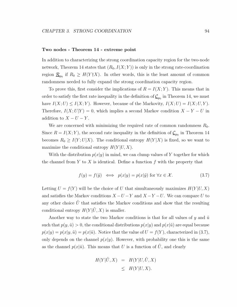
CHAPTER 3. STRONG COORDINATION 94
Two nodes - Theorem 14 - extreme point
In addition to characterizing the strong coordination capacity region for the two-node
network, Theorem 14 states that (R0, I(X; Y )) is only in the strong rate-coordination
region Rp0if R0 ≥ H(Y †X). In other words, this is the least amount of common
randomness needed to fully expand the strong coordination capacity region.
To prove this, first consider the implications of R = I(X; Y ). This means that in
order to satisfy the first rate inequality in the definition of Cp0in Theorem 14, we must
have I(X; U) ≤ I(X; Y ). However, because of the Markovity, I(X; U) = I(X; U, Y ).
Therefore, I(X; U |Y ) = 0, which implies a second Markov condition X − Y − U in
addition to X − U − Y .
We are concerned with minimizing the required rate of common randomness R0.
Since R = I(X; Y ), the second rate inequality in the definition of Cp0in Theorem 14
becomes R0 ≥ I(Y ; U |X). The conditional entropy H(Y |X) is fixed, so we want to
maximize the conditional entropy H(Y |U, X).
With the distribution p(x|y) in mind, we can clump values of Y together for which
the channel from Y to X is identical. Define a function f with the property that
f(y) = f(y) ⇐⇒ p(x|y) = p(x|y) for ∀x ∈ X . (3.7)
Letting U = f(Y ) will be the choice of U that simultaneously maximizes H(Y |U, X)
and satisfies the Markov conditions X−U −Y and X−Y −U . We can compare U to
any other choice U that satisfies the Markov conditions and show that the resulting
conditional entropy H(Y |U , X) is smaller.
Another way to state the two Markov conditions is that for all values of y and u
such that p(y, u) > 0, the conditional distributions p(x|y) and p(x|u) are equal because
p(x|y) = p(x|y, u) = p(x|u). Notice that the value of U = f(Y ), characterized in (3.7),
only depends on the channel p(x|y). However, with probability one this is the same
as the channel p(x|u). This means that U is a function of U , and clearly
H(Y |U , X) = H(Y |U, U, X)
≤ H(Y |U, X).
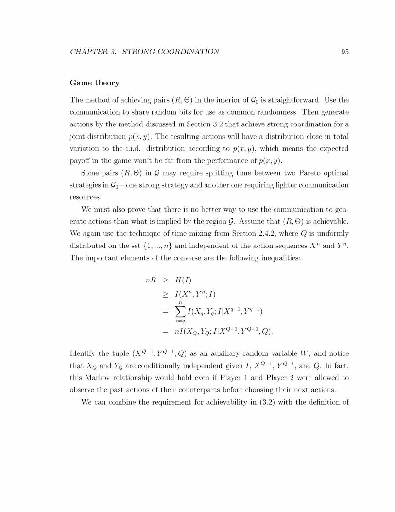
CHAPTER 3. STRONG COORDINATION 95
Game theory
The method of achieving pairs (R, Θ) in the interior of G0 is straightforward. Use the
communication to share random bits for use as common randomness. Then generate
actions by the method discussed in Section 3.2 that achieve strong coordination for a
joint distribution p(x, y). The resulting actions will have a distribution close in total
variation to the i.i.d. distribution according to p(x, y), which means the expected
payoff in the game won’t be far from the performance of p(x, y).
Some pairs (R, Θ) in G may require splitting time between two Pareto optimal
strategies in G0—one strong strategy and another one requiring lighter communication
resources.
We must also prove that there is no better way to use the communication to gen-
erate actions than what is implied by the region G. Assume that (R, Θ) is achievable.
We again use the technique of time mixing from Section 2.4.2, where Q is uniformly
distributed on the set 1, ..., n and independent of the action sequences Xn and Y n.
The important elements of the converse are the following inequalities:
nR ≥ H(I)
≥ I(Xn, Y n; I)
=n∑
i=q
I(Xq, Yq; I|Xq−1, Y q−1)
= nI(XQ, YQ; I|XQ−1, Y Q−1, Q).
Identify the tuple (XQ−1, Y Q−1, Q) as an auxiliary random variable W , and notice
that XQ and YQ are conditionally independent given I, XQ−1, Y Q−1, and Q. In fact,
this Markov relationship would hold even if Player 1 and Player 2 were allowed to
observe the past actions of their counterparts before choosing their next actions.
We can combine the requirement for achievability in (3.2) with the definition of
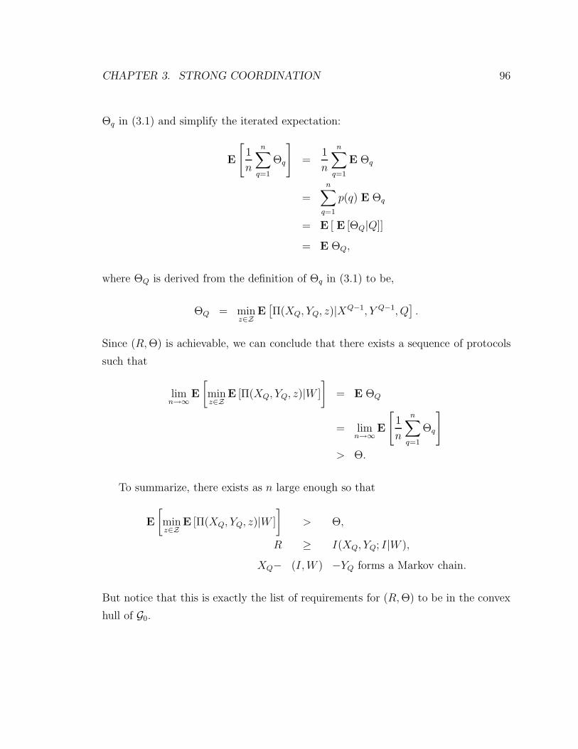
CHAPTER 3. STRONG COORDINATION 96
Θq in (3.1) and simplify the iterated expectation:
E
[1
n
n∑
q=1
Θq
]=
1
n
n∑
q=1
E Θq
=
n∑
q=1
p(q) E Θq
= E [ E [ΘQ|Q]]
= E ΘQ,
where ΘQ is derived from the definition of Θq in (3.1) to be,
ΘQ = minz∈Z
E[Π(XQ, YQ, z)|XQ−1, Y Q−1, Q
].
Since (R, Θ) is achievable, we can conclude that there exists a sequence of protocols
such that
limn→∞
E
[minz∈Z
E [Π(XQ, YQ, z)|W ]
]= E ΘQ
= limn→∞
E
[1
n
n∑
q=1
Θq
]
> Θ.
To summarize, there exists as n large enough so that
E
[minz∈Z
E [Π(XQ, YQ, z)|W ]
]> Θ,
R ≥ I(XQ, YQ; I|W ),
XQ− (I, W ) −YQ forms a Markov chain.
But notice that this is exactly the list of requirements for (R, Θ) to be in the convex
hull of G0.
Chapter 4
Extension
Rather than inquire about the possibility of moving data in a network, we have asked
for the set of all achievable joint distribution on actions at the nodes. For some
three-node networks we have fully characterized the answer to this question, while
for others we have established bounds.
Some of the results discussed in this work extend nicely to larger networks. Con-
sider for example an extended cascade network shown in Figure 4.1, where X is given
randomly by nature and Y1 through Yk−1 are actions based on a cascade of com-
munication. Just as in the cascade network of Section 2.2.3, we can achieve rates
Ri ≥ I(X; Yi, ..., Yk) for empirical coordination by sending messages to the last nodes
in the chain first and conditioning later messages on earlier ones. These rates meet the
cut-set bound. We now can make an interesting observation about assigning unique
tasks to nodes in such a network. Suppose k tasks are to be completed by the k nodes
in this cascade network, one at each node. Node X is assigned a task randomly, and
the communication in the network is used to assign a permutation of all the tasks to
the nodes in the network. The necessary rates in the network are Ri ≥ log(ki). The
sum of all the rates in the network, for large k, is then approximately Rtotal ≥ k nats,
where k is the number of tasks and nodes in the network.
Now consider the same task assignment scenario for an extended broadcast net-
work shown in Figure 4.2. Here again X is given randomly by nature, but Y1 through
Yk−1 are actions based on individual messages sent to each of the nodes. Again, we
97
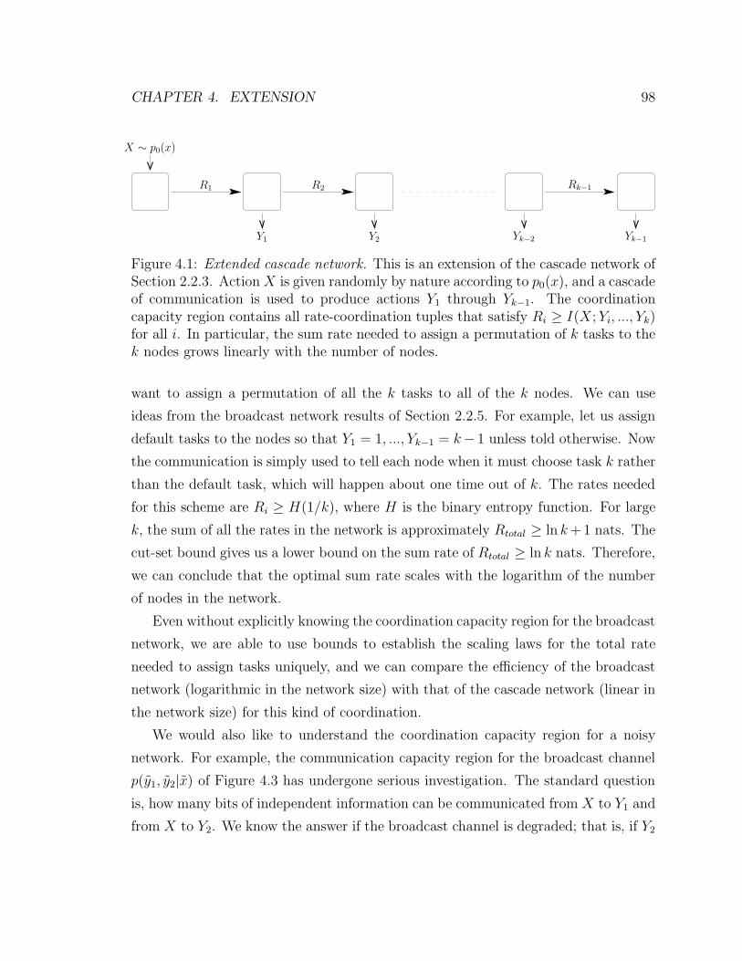
CHAPTER 4. EXTENSION 98replacemen
R1 R2 Rk−1
X ∼ p0(x)
Y1 Y2 Yk−2 Yk−1
Figure 4.1: Extended cascade network. This is an extension of the cascade network ofSection 2.2.3. Action X is given randomly by nature according to p0(x), and a cascadeof communication is used to produce actions Y1 through Yk−1. The coordinationcapacity region contains all rate-coordination tuples that satisfy Ri ≥ I(X; Yi, ..., Yk)for all i. In particular, the sum rate needed to assign a permutation of k tasks to thek nodes grows linearly with the number of nodes.
want to assign a permutation of all the k tasks to all of the k nodes. We can use
ideas from the broadcast network results of Section 2.2.5. For example, let us assign
default tasks to the nodes so that Y1 = 1, ..., Yk−1 = k− 1 unless told otherwise. Now
the communication is simply used to tell each node when it must choose task k rather
than the default task, which will happen about one time out of k. The rates needed
for this scheme are Ri ≥ H(1/k), where H is the binary entropy function. For large
k, the sum of all the rates in the network is approximately Rtotal ≥ ln k +1 nats. The
cut-set bound gives us a lower bound on the sum rate of Rtotal ≥ ln k nats. Therefore,
we can conclude that the optimal sum rate scales with the logarithm of the number
of nodes in the network.
Even without explicitly knowing the coordination capacity region for the broadcast
network, we are able to use bounds to establish the scaling laws for the total rate
needed to assign tasks uniquely, and we can compare the efficiency of the broadcast
network (logarithmic in the network size) with that of the cascade network (linear in
the network size) for this kind of coordination.
We would also like to understand the coordination capacity region for a noisy
network. For example, the communication capacity region for the broadcast channel
p(y1, y2|x) of Figure 4.3 has undergone serious investigation. The standard question
is, how many bits of independent information can be communicated from X to Y1 and
from X to Y2. We know the answer if the broadcast channel is degraded; that is, if Y2
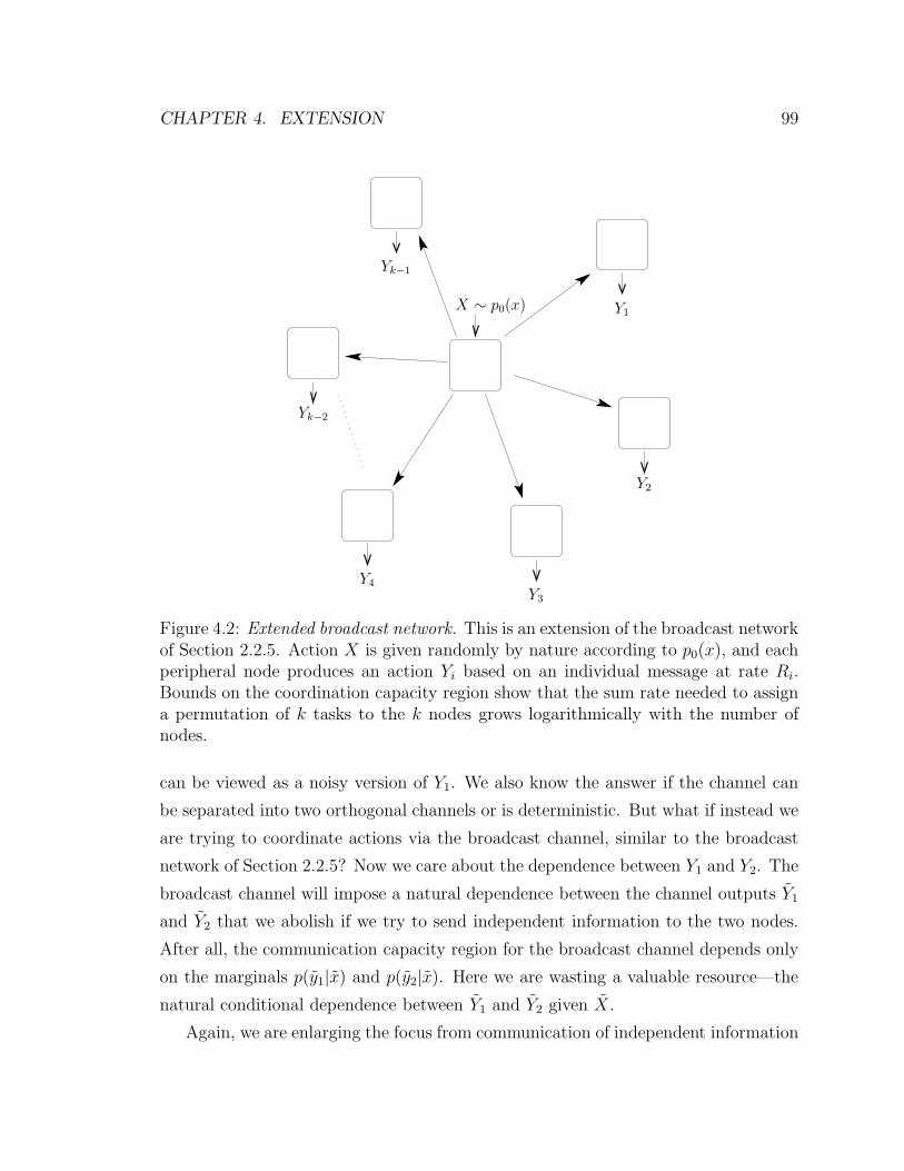
CHAPTER 4. EXTENSION 99
X ∼ p0(x) Y1
Y2
Y3
Y4
Yk−2
Yk−1
Figure 4.2: Extended broadcast network. This is an extension of the broadcast networkof Section 2.2.5. Action X is given randomly by nature according to p0(x), and eachperipheral node produces an action Yi based on an individual message at rate Ri.Bounds on the coordination capacity region show that the sum rate needed to assigna permutation of k tasks to the k nodes grows logarithmically with the number ofnodes.
can be viewed as a noisy version of Y1. We also know the answer if the channel can
be separated into two orthogonal channels or is deterministic. But what if instead we
are trying to coordinate actions via the broadcast channel, similar to the broadcast
network of Section 2.2.5? Now we care about the dependence between Y1 and Y2. The
broadcast channel will impose a natural dependence between the channel outputs Y1
and Y2 that we abolish if we try to send independent information to the two nodes.
After all, the communication capacity region for the broadcast channel depends only
on the marginals p(y1|x) and p(y2|x). Here we are wasting a valuable resource—the
natural conditional dependence between Y1 and Y2 given X.
Again, we are enlarging the focus from communication of independent information
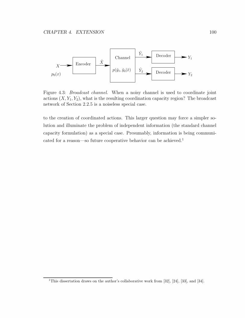
CHAPTER 4. EXTENSION 100
X
Y2
Y1
X
Y2
Y1
Encoder
Decoder
DecoderChannel
p(y1, y2|x)p0(x)
Figure 4.3: Broadcast channel. When a noisy channel is used to coordinate jointactions (X, Y1, Y2), what is the resulting coordination capacity region? The broadcastnetwork of Section 2.2.5 is a noiseless special case.
to the creation of coordinated actions. This larger question may force a simpler so-
lution and illuminate the problem of independent information (the standard channel
capacity formulation) as a special case. Presumably, information is being communi-
cated for a reason—so future cooperative behavior can be achieved.1
1This dissertation draws on the author’s collaborative work from [32], [24], [33], and [34].
Bibliography
[1] R. Ahlswede, N. Cai, S.-Y. Li, and R. Yeung. Network information flow. IEEE
Trans. on Info. Theory, 46(4):1204–1216, July 2000.
[2] J. Tsitsiklis, D. Bertsekas, and M. Athans. Distributed asynchronous determinis-
tic and stochastic gradient optimization algorithms. IEEE Trans. on Automatic
Control, 31(9):803–812, Sept. 1986.
[3] L. Xiao, S. Boyd, and S.-J. Kim. Distributed average consensus with least-mean-
square deviation. Journal of Parallel and Distributed Computing, 67(1):33–46,
Jan. 2007.
[4] B. Bollobas. The Art of Mathematics: Coffee Time in Memphis. Cambridge
University Press, 2006.
[5] A. Yao. Some complexity questions related to distributive computing(preliminary
report). In ACM Symposium on Theory of Computing, pages 209–213, 1979.
[6] A. Orlitsky and A. El Gamal. Average and randomized communication com-
plexity. IEEE Trans. on Info. Theory, 36(1):3–16, Jan. 1990.
[7] O. Ayaso, D. Shah, and M. Dahleh. Distributed computation under bit con-
straints. In IEEE Conference on Decision and Control, pages 4837–4842, Dec.
2008.
[8] V. Anantharam and V. Borkar. Common randomness and distributed control; a
counterexample. Systems and Control Letters, 56:568–572, 2007.
101
BIBLIOGRAPHY 102
[9] H. Barnum, C. Caves, C. Fuchs, R. Jozsa, and B. Schumacher. On quantum
coding for ensembles of mixed states. Journal of Physics A: Mathematical and
General, 34:6767–6785, 2001.
[10] G. Kramer and S. Savari. Communicating probability distributions. IEEE Trans.
on Info. Theory, 53(2):518–525, Feb. 2007.
[11] T. Weissman and E. Ordentlich. The empirical distribution of rate-constrained
source codes. IEEE Trans. on Info. Theory, 51(11):3718–3733, Nov. 2005.
[12] T.S. Han and S. Verdu. Approximation theory of output statistics. IEEE Trans.
on Info. Theory, 39(3):752–772, May 1993.
[13] C. Bennett, P. Shor, J. Smolin, and A. Thapliyal. Entanglement-assisted capacity
of a quantum channel and the reverse shannon theorem. IEEE Trans. on Info.
Theory, 48(10):2637–2655, Oct. 2002.
[14] C. Shannon. Coding theorems for a discrete source with fidelity criterion. In
R. Machol, editor, Information and Decision Processes, pages 93–126. 1960.
[15] H. Yamamoto. Source coding theory for cascade and branching communication
systems. IEEE Trans. on Info. Theory, 27:299–308, May 1981.
[16] A. Kaspi and T. Berger. Rate-distortion for correlated sources with partially
separated encoders. IEEE Trans. on Info. Theory, 28:828–840, Nov. 1982.
[17] J. Barros and S. Servetto. A note on cooperative multiterminal source coding.
In Conference on Information Sciences and Systems, March 2004.
[18] Z. Zhang and T. Berger. New results in binary multiple descriptions. IEEE
Trans. on Info. Theory, 33:502–521, July 1987.
[19] T. Berger. Multiterminal source coding. In G. Longo, editor, Information Theory
Approach to Communications, pages 171–231. CISM Course and Lecture, 1978.
BIBLIOGRAPHY 103
[20] D. Vasudevan, C. Tian, and S. Diggavi. Lossy source coding for a cascade
communication system with side-informations. In Allerton Conference on Com-
munication, Control, and Computing, Sep. 2006.
[21] W. Gu and M. Effros. On multi-resolution coding and a two-hop network. In
Data Compression Conference, 2006.
[22] M. Bakshi, M. Effros, W. Gu, and R. Koetter. On network coding of independent
and dependent sources in line networks. In IEEE International Symp. on Info.
Theory, Nice, 2007.
[23] A. Wyner and J. Ziv. The rate-distortion function for source coding with side
information at the decoder. IEEE Trans. on Info. Theory, 22(1):1–10, Jan. 1976.
[24] P. Cuff, H. Su, and A. El Gamal. Cascade multiterminal source coding. In IEEE
International Symp. on Info. Theory, Seoul, 2009.
[25] A. Orlitsky and J. Roche. Coding for computing. IEEE Trans. on Info. Theory,
47(3):903–917, March 2001.
[26] T. Cover and J. Thomas. Elements of Information Theory. Wiley, New York,
2nd edition, 2006.
[27] I. Csiszar and J. Korner. Information Theory: Coding Theorems for Discrete
Memoryless Systems. Academic, New York, 1981.
[28] Y. Steinberg and S. Verdu. Simulation of random processes and rate-distortion
theory. IEEE Trans. on Info. Theory, 42(1):63–86, Jan. 1996.
[29] A. Wyner. The common information of two dependent random variables. IEEE
Trans. on Info. Theory, 21(2):163–179, March 1975.
[30] P. Gacs and J. Korner. Common information is far less than mutual information.
Problems of Control and Info. Theory, 2:149–162, Jan. 1973.
BIBLIOGRAPHY 104
[31] I. Devetak, A. Harrow, P. Shor, A. Winter, and C. Ben-
nett. Quantum reverse shannon theorem. Presentation:
http://www.research.ibm.com/people/b/bennetc/QRSTonlineVersion.pdf,
2007.
[32] P. Cuff. Communication requirements for generating correlated random vari-
ables. In IEEE International Symp. on Info. Theory, pages 1393–1397, Toronto,
2008.
[33] T. Cover and H. Permuter. Capacity of coordinated actions. In IEEE Interna-
tional Symp. on Info. Theory, Nice, 2007.
[34] P. Cuff, H. Permuter, and T. Cover. Coordination capacity. In preparation,
2009.