Communications Equipment: What Has Happened to Prices? June 2003 Mark Doms Federal Reserve Bank of San Francisco Mark.doms@sf.frb.org The author thanks Neal Dunnay of KMI and Brian Van Steen of RHK for providing data and technical guidance and suggestions. Andrew Batchelor, Niels Burmester, Jon Eller, Susan Polatz, Brigitte van Beuzekom, Courtney Coker, and Margaret Macleod provided research assistance. The author also thanks Carol Corrado, Dan Sichel, Matt Shapiro, for input and advice, and Christopher Greene for editorial comments.

I. Introduction Measuring prices for classes of goods that exhibit rapid rates of technological change raises

special challenges. Over the past several decades, new techniques and data sources have been

developed to in response to these challenges. In fact, an extraordinary amount of attention has

been placed on accurately measuring computer prices and the results of these efforts have been

incorporated into the National Income and Product Accounts (NIPAs).1 Attention was focused

on computers because price declines for computers were easily observed and computers were a

growing share of total investment.

One area where there has been rapid technological change but relatively little effort in terms

of measuring prices is communications equipment. This is surprising since breakthroughs in

communications technology have been a necessary ingredient in constructing the “new

economy”, as witnessed by the widespread use and growth of the Internet, the creation of office

networks, the ability to transmit huge amounts of information over a global fiber optic network,

the increased use of cell phones, the increased capacity of cable television networks, and so on.

Despite the breathtaking advances in communications equipment, the official price indexes

for communications equipment from the Bureau of Labor Statistics (BLS) have barely changed

over the past decade. According to the BLS, producer prices for communications equipment

increased an average of 0.2 percent between 1991 and 2000.2 The prices for communications

equipment stand in stark contrast to those for computers where BLS shows prices falling an

average of 14.5 percent over this period. The Bureau of Economic Analysis (BEA) measure for

computers shows prices falling 17.6 percent.3

Prices of communications equipment, by contrast, have received scant attention. There are

several reasons why research has not progressed more quickly in the field of communication

equipment prices relative to computer prices. First, communications equipment covers a more

diverse set of products than computers. Communications equipment covers such diverse--and

arcane--items as cell phones, alarm systems, fiber optic gear, and local area network (LAN)

equipment. Second, obtaining data on communication equipment prices is more difficult than it

is for computers. Large chunks of communications equipment are sold to relatively few

1 For a summary, see Triplett (2001). 2 The producer price index (PPI) for industry 366 increased at an annual rate of 1.1 percent between 1990 and 1997. Between 1997 and 2000, the PPI fell at an annual rate of 1.2 percent. 3 The BEA measure for computers used to rely on its own measure of prices for larger computers, and the BEA price series fell faster than the comparable BLS series. Consequently, the BEA computer deflator falls faster than BLS’s.

1

customers (for instance, telecom service providers), and prices are not regularly published in

periodicals such as Computer Shopper.

Table 1 shows some measures of both computer and communications equipment investment

in the 1990s. Line 3 shows that the growth rates in nominal investment for computers and

communications equipment were remarkably similar during the 1990s. Additionally, there is

also an eerie resemblance in the level of investment spending in computer and communications

equipment. These facts make it all the more surprising that more research has not been

conducted on the prices of communications equipment.

As mentioned before, the biggest difference between the official investment statistics on

communications equipment and computers is what has happened to official prices. As shown on

line 7 of table 1, BEA’s official prices for computers fell 17.6 percent on average during the

1990s, whereas communications equipment prices fell an average of 2.1 percent. One reason

why the BEA’s official prices for communications equipment falls faster than the BLS PPI is

that the BEA has incorporated alternative price measures for two communications equipment

components. The first is for central office switching equipment, where Grimm (1997) found that

prices fell an average of 9.1 percent per year. The second is for local area network (LAN)

equipment, where Chris Forman and I found that prices fell an average of 17.5 percent per year

between 1995 and 2000.4

Why do I care about communications equipment prices, or, why do I think a priori that

communications equipment prices fell faster than the BLS data would lead us to believe? First,

the small handful of studies that have examined portions of communications equipment have

found that prices have fallen quickly, but perhaps not as much as computers. With that said,

these studies did not look at a random sample of the communications equipment universe, and

they also have not examined the areas where technological change has been most rapid. Second,

as stated earlier in the introduction, there are numerous instances of technological change in

several parts of the communications equipment spectrum that have revolutionized

communication services. Third, as just discussed, big bucks have been spent on communications

equipment, so deriving more accurate measures of prices would likely have consequences for

top-line measures of economic activity. For instance, Jorgenson and Stiroh (2000) go so far as to

run simulations under different scenarios for communications equipment prices.

4 See Doms and Forman (2003).

2

To illustrate the potential importance of deriving more accurate measures of communications

equipment, table 2 shows the contributions of computers and communication equipment to gross

domestic product (GDP) and equipment and software (E&S) growth during the 1990s.5 Line 2

shows that computer investment contributed an average of almost 0.3 percentage point to the

average annual growth rate of GDP during the last decade, with a larger contribution in the

second half of the 1990s. In contrast, communications equipment investment contributed only

about a third as much as computers did. A similar pattern holds for E&S spending.

Given the similar nominal shares and growth rates of computers and communications

equipment, it seems that the potential payoff of “fixing” communications equipment prices

relative to the cost of doing so may be high. The question then arises of how can we accurately

measure prices of communications equipment? This paper pursues the following, albeit

imperfect, approach. First, I map out the different types of communications equipment and how

spending on these different types have changed over the years. The National Income and

Product Accounts (NIPA) data for communications equipment is very aggregated, so I use a slew

of information from other sources on the types of communications equipment purchased. These

data help identify those areas within the communications equipment sector where spending is

large and where it has accelerated. This analysis is in the second section of the paper.

The third section presents information from past studies on communications equipment

pricing. The fourth and fifth sections of the paper can be viewed as continuations of the “house-

to-house combat” to improve price measures used in the NIPAs (see Shapiro and Wilcox

(1996)). Section four presents new results on the prices of modems and public telephone

exchanges (PBX). The fifth section delves into fiber optic equipment, the area where

technological change has been extremely rapid and spending accelerated sharply in the late

1990s and 2000. In the sixth section, the information developed in this paper is combined with

the results from elsewhere to come up with several overall price indexes for communications

equipment.

Finally, the seventh section addresses how these alternative price indexes would affect

growth rates in various investment categories and how calculations on capital deepening and

multi-factor productivity (MFP) would change.

5 The communication equipment GDP calculations were performed by using E&S communication equipment spending and estimates of government and consumer spending. The government and consumer spending estimates were based on the 1992 input-output tables, the last official estimates. The data were further adjusted for imports and exports.

3

II. What is Communications Equipment? Communications equipment comprises most of the equipment that sends and receives

information and the vast array of types of equipment that lies between the sender and receiver.

Over time, the types of equipment have multiplied--instead of copper wires connecting homes to

central switching offices, equipment now exists that sends information over fiber optic networks,

satellites, and cell phone towers, in addition to the equipment that make computer networks run.

How to classify all of this equipment is therefore a daunting task. The Standard Industrial

Classification (SIC) system, and the more recent North American Industrial Classification

System (NAICS), break down communications equipment into several subcategories: telephone

apparatus manufacturing, radio and television broadcasting and wireless communications

equipment manufacturing, and other communications equipment manufacturing. Although these

categories are useful, over the years there has been movement away from the traditional modes

of communication that these systems were based (namely, the land-line telephone system).

Indeed, the industry seems to assign communications equipment into much different categories.

To help explain what constitutes communications equipment and to help us think about how the

types of equipment should be classified, figure 1 presents a simplified diagram of

communications networks.

The way to view figure 1 is that information is sent from the left-hand side of the diagram to

the right-hand side. The items listed on the left are those pieces of equipment that initially send

out a message, and the pieces of equipment listed on the far right are those that receive the

message. The items in the middle are the necessary equipment a message must traverse to get

from the sender to the receiver. The diagram focuses on voice and data networks and omits

radio, TV, alarm systems, walkie-talkies, and defense- specific communications equipment.

With that said, the equipment shown in figure 1 makes up the bulk of communications

equipment spending.

The elements on the left-hand side are broken into voice and data. The split between voice

and data transmission has arisen because a premium has been placed on the quality of the voice

network. When a voice message is transmitted, it is essential that each part of that message

arrives at its final destination in the correct order and in a timely manner. Therefore, the

4

resources devoted to sending a voice message are greater than the resources required for sending

a comparably sized data transmission.6

On the left side of figure 1, there are three elements under the voice heading and just one

element (computer) under the data heading. Each of these systems has evolved somewhat

separately, and each has its own protocols and formats. Even as I write this paper, these

distinctions are blurring. For instance, cell phones are being used to transfer data (systems such

as BlackBerry and Verizon’s Express Network), and phone calls can be made over computer

networks. With that said, the connections shown in figure 1 represent the routes that a majority

of voice and data traffic travels.

Once the information leaves the original sending piece of equipment (phone, cell phone,

business phone, or computer), the information is usually sent to a location where information

from several sources congregates before being sent on the next leg of its journey. This system is

akin to the hub-and-spoke system of the airlines. The hub-and-spoke system is used because it is

not economical to have direct connections between everyone on a network to everyone else on a

network. Therefore, a good chunk of communications equipment spending is on equipment that

takes in many signals and makes and decides where to send the signals to next. Over time, the

equipment that performs this routing function has become ever more complex and able to handle

greater volumes of information.

Examples of this type of equipment are listed in the middle of figure 1. The upper left

portion of figure 1 shows that most home phones are connected to a local telephone-switching

center, usually by copper wire.7 Cell phones instead send a signal over the airwaves to a base

station. The signals in the base station are then sent to a switching center, joining calls made

from residences. Phones in businesses, government buildings, and academic institutions are

often connected to their own phone network. The two dominant types of equipment that run

these networks are called public branch exchange (PBX) and keystone telephone systems (KTS).

PBXs and KTSs are then usually connected to switching centers.

In figure 1, the fourth device used to initially transmit information is the computer. Actually,

the parts of the computer that are officially considered communications equipment are modems

6 However, as technology improves, the distinction between voice and data transmission will all but disappear. Already, voice over Internet protocol (VOIP) applications are arising. In the IP system, a message is broken into packets, and those packets are then routed to their final destination, although not all of the packets will take the same route. 7 Switching centers are also referred to as central offices, local central office, exchange, and local exchanges. Also, a home phone may transmit and receive information over its cable TV line.

5

and local area network (LAN) cards (the most common of which are Ethernet cards). A

computer can be linked to larger networks in one of three ways. First, with a traditional analog

modem or a digital subscriber line (DSL), a computer can use a copper phone line to connect to a

switching center. Second, computers can use cable TV lines. These first two mediums are

popular for home computer use. Many business, government, and academic computers are

instead linked to a LAN. LANs can then be linked to other LANs, to switching centers (say, via

a T1 line), or to wide area networks (WANs).

Switching centers contain various equipment, including telephone equipment, satellite dishes,

and the equipment to light up fiber optic networks. A message sent from the right side of figure

1 to the left side may go through many such switch centers. For data communication, a message

is broken into packets, and those packets can each take different routes to get to the final

destination.

Expenditures Figure 1 shows the basic components of the modern communications system. Using data from a

very wide variety of sources, table 3 shows estimates of how much was spent on various pieces

of equipment.8 The data in table 3 come from a very wide array of sources, mainly from private

research firms and trade associations. For instance, the data on expenditures on LAN equipment

came from Gartner/Dataquest, the data on expenditures for fiber optic equipment came from two

firms that follow the industry—and is described in more detail later in the paper-- and data on

many of the smaller categories came from various issues of the Multimedia Telecommunications

Market Review and Forecast by the Telecommunications Industry Association.

The data in table 3 are only from 1997 to 2000 because those are the years for which I could

obtain decent estimates for all major categories. In some of the results that follow, results for

individual pieces of equipment go back until the late 1980s and there are some results for 2001.

I chose private and industry sources over government sources for two reasons. First,

government statistics do not report the necessary detail on how much is spent on different types

of communications equipment. Second, private sources tend to classify communications

equipment differently than the SIC and NAICS, and since I have to rely on private sources to

estimate price indexes, I chose the categories that the industry uses.

8 The largest omitted categories in table 3 are likely radio equipment (outside of cellular phone equipment), broadcast and studio equipment, and alarm systems.

6

Most categories experienced growth in nominal spending in the late 1990s. In particular,

there was a tremendous surge in spending on fiber optic equipment (the fiber itself is relatively

cheap and not considered communications equipment), reflecting a large build-out of the several

large new fiber networks. Fiber optic networks and fiber optic equipment is discussed more fully

in section V.

Table 3 also shows where the big bucks are spent on communications equipment. Spending

on communications equipment is dispersed among many distinct types of products. The largest

single major category is switching-center equipment. And within that category, fiber optic

equipment made up the bulk of the expenditures in 2000 (in 1997, the share of central office

switching equipment was only half as large). This fact is interesting since there have been many

reports of the tremendous advances made in fiber optic technology. But just how important

those advances are to all of communications equipment does depend on how much is spent on

fiber optics.

The bottom of table 3 shows the total expenditures in the categories I’ve displayed. The

bottom of table 3 also shows communications equipment investment as reported in the NIPAs.

The sums of my categories are less than the NIPAs because I have excluded a number of

categories. However, what is somewhat reassuring is that the data I’ve tallied has similar growth

rates to the NIPA data between 1997 and 2000, and both series show an especially large increase

in 2000.

III. Previous research on prices of communications equipment There has already been research on prices for some of the categories shown in table 3. In

particular, research has been done on cell phones, central office telephone switches, and LAN

equipment. Together, these three categories constitute 42 percent of the communications

equipment expenditures in 1997 and 36 percent 2000. Because one objective of this paper is to

devise a best guess for an overall price index, I’ll discuss the previous research with an emphasis

on what were the driving forces that lowered prices. The results from the previous studies are

summarized in table 4.

Cell Phones

Jerry Hausman has written a series of papers on the price of cellular telephone service. He cites

that when cell phones were first introduced in 1983, they sold for about $3,000. By 1997, they

7

sold for about $200. These are very rough numbers, and it is certain that the average cellular

phone in 1997 had a better feature set than an average phone in 1983. With that said, using the

Hausman quotes, prices for cellular phones fell an average of 17.0 percent between 1983 and

1997. One of the primary reasons for the drop in the price of cell phones has been the advances

made in semiconductors. Cell phones are quite complex devices, and it has been said that if a

cell phone were made with vacuum tubes, the cell phone would have to be the size of the

Washington Monument. An additional factor that may help explain the drop in cell phone prices

is economies of scale in production of the phones and its components. In 2000, there were an

estimated 400 million cell phones sold worldwide.

Telephone Switches

Kenneth Flamm(1989) and Bruce Grimm (1997) have examined prices of telephone switches.

Telephone switches are pieces of equipment usually installed in “switching centers” that route

calls from one center to another and then to the final destination. The first telephone switches

were electromechanical; these switches physically moved to complete a circuit over which a

conversation could be held. In the early 1980s, digital electronic telephone switches performed

the same function, but without moving parts. The new switches could perform other functions as

well. Bruce used data from the Federal Communications Commission (FCC) to run a hedonic

regression where the price of the switch was regressed on a number of explanatory variables. He

found that between 1985 and 1996, prices fell an average of 9.1 percent. However, in the later

years of his study, he found that prices fell an average of 16.1 percent.

LAN Equipment

Chris Forman and I examined the prices of different types of LAN equipment in the second half

of the 1990s. LAN equipment is the equipment that sends and routes information over computer

networks. The development of this equipment has made accessing the Internet and e-mailing

more affordable. Within the LAN equipment aggregate, there are four primary components:

LAN cards (the card in a computer that sends and receives information on a computer network),

switches (devices that perform simple routing functions), routers (devices that often sit atop

computer networks and determine where information packets should be sent), and hubs (pieces

of equipment that act as traffic cops in merging information onto a computer network).

8

Forman and I found that prices for LAN equipment fell far faster than the BLS comparable

PPI would suggest--between 1995 and 2000, the prices for LAN equipment fell at a 17.5 percent

annual rate, compared with the comparable PPI that fell only 0.1 percent. As shown in table 4,

prices did not fall evenly across the different types of LAN components.9

The aforementioned studies found that prices for various types of communications equipment

fell, and fell considerably faster over the time periods examined in contrast to the most

comparable PPIs. However, making an inference to total communications equipment from these

groups is not prudent, as these groups make up just 36 percent of communications equipment

spending in 2000. Also, there is a question of whether these studies represent a random sample

of communications equipment. They probably do not.

One of the objectives of this section is to provide some evidence that prices for

communications equipment fell faster than the official statistics indicate. The studies mentioned

before certainly provide some evidence. Some other indirect evidence might also shed light on

the issue, namely a measure of the rate of innovation within the communications equipment

industry and of the prices for inputs of semiconductors. The first information presented is on

patents, and the second set of information comes from Aizcorbe, Flamm, and Khurshid (2002)

on price comparisons of semiconductors used in computers versus those used in communications

equipment.

A contributing factor to the marvelous improvements in technology has been the rapid pace

of scientific discoveries in the fields of computers, communications equipment, and

semiconductors. Devising metrics that somehow capture the rate of technological progress is

difficult. Two commonly used measures are patents and research and development (R&D)

spending. Unfortunately, R&D spending figures by industry are not published at a fine enough

level of detail (communications equipment, SIC industry 366, is sometimes lumped in with other

industries in industry 36, such as semiconductors [SIC industry 367]). However, Manuel

Trajtenberg of Tel-Aviv University maintains a database of patents, and those patents are

9 Why did prices of LAN equipment fall so quickly? The reasons are interrelated and speculative, and they include the degree of competition, simplicity of the product, the size of the market, and how many of the devices are made. In terms of competition, prices fell fastest for home and small office routers, the segment of the router market with the most competition (this is the segment where Cisco, the dominant maker of routers, has the smallest market share). One reason for the high level of competition is that designing and producing low-end routers is relatively easy, so that many firms can enter. Also, the quantity of low-end routers allows producers to enjoy economies of scale in production of the routers themselves and in the production of the semiconductors used in the routers. Because of steep competition, prices for switches also fell quickly. Again, although Cisco dominates the market, it did not do so initially.

9

assigned to classes. Figure 2 shows the percent of total patents that are awarded to three high-

technology fields--computers, communications equipment, and semiconductors--between 1963

and 1999. The share of patents in the computers and peripheral equipment category has been

increasing much faster than that of the other two categories. Also, the share of total patents

going to communications equipment has been increasing. One wildcard is how the patents for

semiconductors are related to chips that are used in computers versus chips that are used in

communications equipment.

One reason to think prices for communications equipment have fallen faster than official

statistics would indicate is that communications equipment is a large consumer of

semiconductors. Aizcorbe, Flamm, and Khurshid have examined the prices of semiconductors

by final use category, examining the semiconductor price indexes for semiconductors that go into

computers, communications equipment, and so on. They find that the content of semiconductors

in communications equipment is about 11 percent. Further, they estimate that in the late 1990s,

prices for chips that went into communications equipment fell, on average, about 30 percent per

year.

So far I have discussed previous studies on communications equipment prices and some

other information that suggests that prices for communications equipment should perhaps be

falling faster than the official statistics indicate, but perhaps not as fast as the official numbers

for computers. The next two sections present new results on three types of communications

equipment to better round out what is actually known about prices.

IV. Modems and PBX/KTS Measuring prices for high-tech goods has received a voluminous amount of attention in the past

two decades. During this time, several techniques have been employed. Two of the more

popular methods are hedonics and match-models. Aizcorbe, Corrado, and Doms (2003) describe

these two methods and when these two methods yield numerically similar results. In the results

presented below and in the results presented in the next section on prices for fiber optic

equipment, matched-model techniques are used. One reason for using matched-model

techniques is because the available data is best suited for matched models. For many of the

products, I do not have access to all of the performance characteristics to estimate a hedonic

model, and I am also constrained by the number of observations. However, as Aizcorbe,

Corrado, and Doms demonstrate, the matched model approach yields numerically similar results

10

to the hedonic approach when net entry of new products is not large. In most of the results

presented in this section and the next, this is indeed the case.

One, albeit small, segment of communications equipment where price information is

available for a large number of products is for modems. This first part of this section analyzes

modem prices. The second part examines prices for PBX/KTS equipment, the internal phone

networks used by many businesses.

Modems Although modems are a small part of communication equipment spending, prices for analog

modems are relatively easy to obtain because they are sold in the same outlets as personal

computers. Examining modems is of interest because there has been tremendous technological

change over the past decade. For instance, in late 1991, 9600 baud analog modems were

introduced, followed by 14400 baud modems in 1992:Q3, and 28800 baud modems in

1994:Q4.10 The rate of increase in speed during this period averaged about 63 percent, a bit less

than Moore’s law. One might suppose that modems are one type of equipment where prices fell

faster than other types of communications equipment because of high competition. Also, it is

possible that since most personal computers (PCs) come equipped with modems, firms have been

able to achieve higher economies of scale than other segments of the communications equipment

industry (modems are similar to LAN cards in many ways).

Our study on modems has two parts. The first part analyzes prices for analog (dial-up)

modems for PCs from 1989 to 1998. The second part looks at cable modems from late 1999 to

late 2001. There are two modem groups that we do not examine, PCMCIA modems (modems

commonly used for laptop computers) and modems used for business applications.

Analog modems. We gathered information on 681 modems from PC World magazine between

1989 and 1998. The reason we stop in 1998 is that finding advertised list prices for modems

became more difficult as modems were increasingly offered as standard equipment in computers.

For consistency, we obtained prices in ads from Computer Direct Warehouse and Arlington

Computer Products, two large retailers of PCs and components that had ads in each issue of PC

World that we examined. Manufacturers of the data collected were US Robotics, Hayes, and 10 A 9600 baud modem is not faster than a 1200 baud modem--the 9600 baud modem has higher capacity. The speed of the signals is dictated by the speed of electricity over copper wires, whereas the signal can be modified and refined to have higher capacity. Although engineers cringe when “higher speed” is used to describe various forms of bandwidth, it is likely they have lost the semantic battle.

11

Practical Peripherals. Our database contains the listed retail price and the speed for each modem.

We matched unique modem models across consecutive quarters. On average, each modem was

in our sample for seven quarters. We calculated the geometric mean of prices in two consecutive

periods.11 Also, we calculated separate price indexes for different classes of modems. For all of

the price indexes shown, we required a minimum of six observations. The overall analog

modem price index is based on an average of about 100 observations.

A problem with using geometric means is that we are treating each observation equally. If

the revenue shares were known for each modem, then we would use that information to construct

a matched-model superlative index. If there is a correlation between prices changes and the size

of the revenue shares, then the geo-means approach yields biased results. For instance,

substitution bias can occur if revenue moves toward those modems where prices are falling

relatively rapidly. Unfortunately, we do not know how many of each type of modem was sold,

and I could not find any information on this subject.

Our results are shown in figure 3. For comparison, we also place the BEA computer price

index on this figure. Our overall modem index falls an average of 15.6 percent over the sample

period, compared with the 16.3 percent drop in the BEA computer deflator. Initially, our price

index falls more slowly than the BEA computer deflator, when 1200 and 2400 baud modems

were commonplace and the 9600 baud modems had not yet been introduced. However, with the

advent of 9600 and 14400 baud modems, prices fell more quickly, especially in the case of the

14400 baud modems. Prices continued to fall, although the rate of decline does vary from period

to period. Of interest is that prices of the 56K modems increased during their first year in our

sample and then quickly fell.12

Figure 4 highlights modems that are over 10K baud. We computed an over-10K-baud index

and compared it with a BLS modem index for this category. Our index fell significantly faster

than the BLS index: between 1994:Q2 and 1998:Q3, our index fell at an average rate of 15.4

percent, compared with 8.7 percent for BLS.

11 Hedonic regressions could not be run because the advertisements did not provide a complete list of the characteristics of the modems. The advertisements always mentioned the speed and the name of the modem but did not mention any of the other characteristics. For instance, modems vary by the software that is included (such as software that allows the user to use the modem as a fax machine), warranty, speakerphone, mike, caller ID, free tech support, and so on. 12 I’m not sure why this is the case. I read that there was some trouble in using these modems initially, and demand may not have been that high. The 56K modems are now standard equipment.

12

Cable modems. In the past several years, adoption of modems for broadband access (DSL and

cable) has increased markedly. We were able to obtain industry-level estimates on revenue and

quantities for cable modems between 1999:Q4 and 2001:Q1. The data come from Gartner, a

private research firm that tracks a number of high-technology industries. The data we were able

to gather are simply the revenue and quantity estimates. According to Gartner, most cable

modems are similar in that they must meet the DOCSIS (Data Over Cable Service Interface

Specification) standard, the standard that defines “the interface requirements for cable modems

involved in high-speed data distribution over cable television system networks” (CableLabs

website, 2002). The characteristics of cable modems over this period are fairly uniform, that is, a

cable modem in 1999 was not that much different from a cable modem in 2001. Using the

Gartner data, the average price of a cable modem fell from $228 in 1999:Q4 to $145 in 2001:Q1,

an average price decline of 30.4 percent. The results for the cable modems are shown in the

upper left of figure 3.13

PBX/KTS My attention now turns to the prices of the phone systems located in many businesses,

government offices, and other sites. One reason to examine this segment is that sales of these

systems exceeded $8 billion in 2000.

These telephone systems allow users to call one another without using central switching

centers. These telephone systems are smart enough to know that when, for instance, you dial a

four-digit code, the call you are placing is to another phone within the system. Sometimes on

these systems, you have to dial a “9” to get an outside line, that is, a line that is most likely

connected to a switching center. These systems fall into two categories: public branch

exchanges (PBX) and keystone telephone systems (KTS). A PBX is a bit more sophisticated

than a KTS in that the number of phone lines entering a location is less than the number of

phones in that location.

PBX and KTS systems have many features, and the feature set has grown over time. Perhaps

this isn’t surprising. Newer features include call forwarding, call waiting, caller ID, plug-in

13 Cable modems are now being increasingly sold in retail stores. Recent prices (March 2002) for DOCSIS cable modems are about $100, a decline of about 30 percent from the year-ago Gartner prices. Only recently are cable and DSL modems sold through retail stores. In 1999 and 2000, cable companies distributed nearly all cable modems.

13

capability to a T1 line, message centers, and so on.14 According to an industry contact, the prices

of additional features have been falling over time. However, this contact also said that getting

price data would be difficult because prices are usually quoted only after a request for a specific

system with specific features has been placed.

I was able to get some data that can produce a bound for prices. Several private firms track

the industry and classify PBX/KTS systems by how many lines they have. These firms have

revenue estimates for “basic” systems. What exactly constitutes a “basic” system has changed

over time, with a “basic” system that is sold today having more features than a “basic” system of

five years ago.

The data on revenue and on average prices is presented in table 5 and come from

Gartner/Dataquest and appear as they are published. That is, there is no underlying detail that I

have access to that is not shown in the table. As shown at the bottom of the table, prices fell an

average of 5 percent between 1994 and 2000. Again, I believe that these estimates, based on the

Gartner data, to be upper bounds--prices likely fell even faster because the basic configurations

improved over time, and my estimates do not pick this up. Just how much are the estimates

biased? I don’t know. However, a vendor of this equipment believed that prices have fallen in

the single digits every year.

V. Fiber Optics The area within communications equipment where the most rapid technological innovations have

occurred within the past several decades is fiber optics. Instead of using electrical signals to

carry messages over copper wires, there has been an increasing move toward using pulses of

light over thin fibers of pure glass. Although there have been improvements in the glass, the

most significant innovations have come in the equipment used to transmit and receive the light

impulses. In this section, I want to provide a brief overview of fiber optics and then present

some information on what has happened to the prices of the equipment used in fiber optic

networks.

14 There is a trend toward converting traditional circuit-based PBXs to Internet Protocol (IP) technology. A UNIX or NT server would run the phone system instead of a PBX. The phone system would become a computer network, and each phone would have an IP address. Although there has been much talk about this technology, sales of IP-based systems have yet to take off.

14

Overview of fiber optics

The use of light in communications has existed for some time, including the use of smoke

signals, “one if by land, two if by sea,” semaphore, and other visual means when there was direct

line of sight. In a development that portended great things to come, Alexander Graham Bell

invented the photophone (figure 5). The photophone is basically a mirror that aims a beam of

light to a receiver. The source of the light is the sun. The photophone has a device that vibrates

a mirror as someone speaks. At the receiving end, a detector picks up the vibrations in the beam

of light and converts the vibrations back into voice (analog technology). The sun is not a reliable

light source, and the photophone now languishes on the shelves of the Smithsonian Institution.

However, using light to carry information has proven to be as revolutionary as the phone itself.

The next big extension of the Bell idea was to transmit light over a medium that didn’t have

to go into a straight line and didn’t require the cooperation of the sun. Between 1850 and 1960, a

series of scientific discoveries led to the use of glass fibers, sheathed in various materials, as a

medium through which to transmit light. In 1960, the laser was invented. Lasers are able to

focus large amounts of light into very tight streams, making them ideal for sending light down a

thin glass fiber strand. Refinements in lasers and fibers continued through the 1960s and 1970s,

and in 1977 the first field trials were conducted that used fiber optic cables to transmit voice calls

in Chicago. There has been near continuous improvement since, especially in terms of the

amount of information that can be transmitted by a beam of light and the number of light waves

that can be simultaneously sent down a piece of glass fiber.

Fiber optic networks are complex and require many different types of equipment. The basic

components of a fiber optic network are the fiber through which the light pulses are sent, a

transmitter, a receiver, and a regenerator. As I mentioned before, the fiber itself is not

considered communications equipment. A transmitter is a device that takes a signal (perhaps an

electrical signal), translates that signal into light pulses, and then sends those light impulses into

a piece of glass fiber. Lasers are often used to send the light. Because the capacity of fiber is

very high, the transmitter is able to take in many signals simultaneously and translate them all

into a single wavelength of light. Taking many signals (tributaries is a word that is used) and

15

merging them into a single data stream is called multiplexing. The devices that take in many

tributaries to produce one stream of information are called multiplexers.15

At the end of the fiber, there is a receiver, called a demultiplexer.16 The demultiplexer

receives the light signal, converts it into electrical signals, and then sends them out to multiple

conduits, the reverse of what happened at the beginning. That’s a simplified version of the

basics.

In 1996 the basics got a bit more complicated, and exciting. Instead of using one laser to

shoot light down a strand of fiber, why not use two or more that operate at different wavelengths

and shoot these beams down the fiber simultaneously? One example of the logic behind why

this technology works is that when you are in a roomful of people talking, you can sometimes

concentrate and just listen to one voice. Your mind acts as a filter and blocks out the other

voices. If too many people are talking, and the voices are similar, then hearing a single voice is

difficult. Just as the voices have to be different, the wavelengths of the lasers also have to be

different. An amazing consequence of this technology (a technology that has been used for a

very long time in sending electrical signals down copper wire) is that the capacity of a single

piece of fiber instantly increases. This technology is called dense wave division multiplexing

(DWDM). The advent of DWDM technology created quite a hoopla, and references are

frequently made to the increased capacity of a piece of fiber because of DWDM. In 1996 (when

only a small handful of DWDM systems were initially deployed commercially), the maximum

amount of information that could be transmitted through a piece of fiber was 2.5 gigabytes per

second (Gb/s). In 2000, DWDM systems could shoot 40 wavelengths, each carrying 2.5 Gb/s,

for a total of 100 Gb/s. In just four years, DWDMs alone increased the potential capacity of a

piece of fiber by a factor of 40, well above the pace of Moore’s law.

Figure 6 provides a simplified version of a long haul fiber optic network (most expenditures

on fiber and fiber optic equipment in the 1990s were on long-haul networks). The central circle

in figure 6 is a fiber ring. Many networks are built using the ring concept--several fibers are

used to connect two points so that data can be transmitted in either direction. If the ring is

15 At a point in the process, electrical signals have to be converted to light, and light converted back to electrical signals. The equipment that does this--often the multiplexers--is very expensive. Over the past several years, there has been research on “all optical” networks, networks that would not need the expensive conversion equipment. 16 Once the pulses of light go merrily down the fiber strand, they begin to disperse somewhat, losing some of the tight form they had initially. This dispersion is called attenuation. At certain intervals, a fiber network may have a “regenerator,” a device that reads in the signal, cleans it up, and sends it out again. I was not able to find any information about regenerators, either in terms of expenditures or in terms of prices and characteristics.

16

severed at one point, the data can be transmitted in the other direction. Various pieces of

equipment are used to send and receive information over fiber. A short fiber optic glossary is

presented in table 6.

In the late 1990s and into 2000, fairly large expenditures were made on the various pieces of

fiber optic equipment. Estimates of these expenditures are presented in table 7, and these

estimates came from either three different private firms; Gartner/Dataquest, RHK, and KMI.

RHK is a private firm that tracks the telecommunications industry and KMI is also a private firm

that specializes in tracking the fiber industry, especially the amount of fiber cable laid.

The table shows that the growth rate in nominal spending on fiber optic equipment has

increased at close to a 20 percent annual rate since 1994.17 A large ramp up in spending for

fiber optic equipment occurred in 1999 and 2000 as a flood of companies rushed into the long-

haul fiber optic business; at the end of 2000, there were 11 companies that had more than 10,000

route miles of fiber. Unfortunately, there was a tremendous amount of duplication on the main

routes and many of the companies went bankrupt. As a consequence, expenditures on fiber optic

gear dropped precipitously in 2001.18

Prices of fiber optic equipment

To reiterate, getting information on prices for fiber optic gear is difficult because there are

relatively few firms that make the stuff and the number of customers is fairly limited as well.

Consequently, standard price catalogs do not exist. An analyst at RHK, Brian Van Steen, tracks

prices and quantities for a large number of pieces of fiber optic gear, and he was kind to share his

results for multiplexers and for DWDM equipment. The information for digital cross connects

came from Gartner. The results that follow are a series of tables that display that data that was

given to me. Each table contains information on a different piece of fiber optic equipment, and

price indexes were formed by using a matched model, superlative index number approach. The

17 The fiber optic cable is not classified as communications equipment according to the SIC and NAICS. Also, the cost of the fiber cable itself is relatively cheap. Estimates are that in 1999 and 2000, about $3 billion was spent annually on the cable. In contrast, expenditures on the equipment used to transmit and receive information over the cable topped $22 billion in 2000. Also, telecom service providers have to invest in other forms of equipment to get a fiber optic network up and going, including computers. 18 The advent of DWDM equipment may have hastened the collapse of several long-haul fiber companies. DWDM has increased the potential capacity of a piece of fiber many fold. Therefore, when demand on a certain fiber route increases, it is relatively easy (that is, cheap) to increase the capacity of the existing line instead of lighting up another fiber. Therefore, not as many fibers are needed to transport a given amount of information.

17

reader can skip ahead several pages to the discussion of table 11 that presents the summary

results for fiber optic equipment.

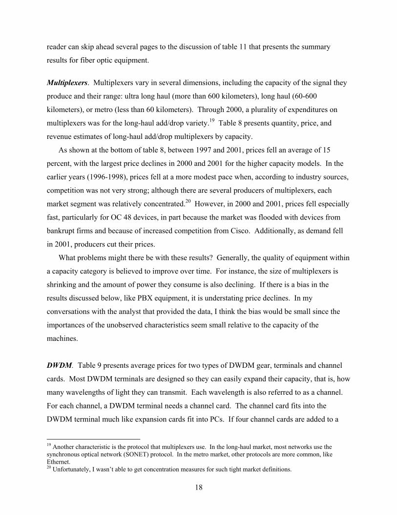
Multiplexers. Multiplexers vary in several dimensions, including the capacity of the signal they

produce and their range: ultra long haul (more than 600 kilometers), long haul (60-600

kilometers), or metro (less than 60 kilometers). Through 2000, a plurality of expenditures on

multiplexers was for the long-haul add/drop variety.19 Table 8 presents quantity, price, and

revenue estimates of long-haul add/drop multiplexers by capacity.

As shown at the bottom of table 8, between 1997 and 2001, prices fell an average of 15

percent, with the largest price declines in 2000 and 2001 for the higher capacity models. In the

earlier years (1996-1998), prices fell at a more modest pace when, according to industry sources,

competition was not very strong; although there are several producers of multiplexers, each

market segment was relatively concentrated.20 However, in 2000 and 2001, prices fell especially

fast, particularly for OC 48 devices, in part because the market was flooded with devices from

bankrupt firms and because of increased competition from Cisco. Additionally, as demand fell

in 2001, producers cut their prices.

What problems might there be with these results? Generally, the quality of equipment within

a capacity category is believed to improve over time. For instance, the size of multiplexers is

shrinking and the amount of power they consume is also declining. If there is a bias in the

results discussed below, like PBX equipment, it is understating price declines. In my

conversations with the analyst that provided the data, I think the bias would be small since the

importances of the unobserved characteristics seem small relative to the capacity of the

machines.

DWDM. Table 9 presents average prices for two types of DWDM gear, terminals and channel

cards. Most DWDM terminals are designed so they can easily expand their capacity, that is, how

many wavelengths of light they can transmit. Each wavelength is also referred to as a channel.

For each channel, a DWDM terminal needs a channel card. The channel card fits into the

DWDM terminal much like expansion cards fit into PCs. If four channel cards are added to a

19 Another characteristic is the protocol that multiplexers use. In the long-haul market, most networks use the synchronous optical network (SONET) protocol. In the metro market, other protocols are more common, like Ethernet. 20 Unfortunately, I wasn’t able to get concentration measures for such tight market definitions.

18

terminal, then that terminal can transmit four different wavelengths simultaneously. As demand

increases, additional channel cards are added as needed. Increasing capacity in this way can be

done quickly. For instance, according to KMI, the average DWDM terminal had a maximum

capacity of 42 channels, but, on average, only 12 of those channels were used. The sales of cards

are quite large--between 1998 and 2001, about 44 percent of DWDM sales was of cards. The

remainder of the expenditures was on the terminals themselves and other miscellaneous

equipment.

RHK has collected some information on prices for various pieces of DWDM gear, and those

are presented in table 9. The first portion of table 9 presents price estimates for a sample of

DWDM terminals. The terminals vary by the number of cards they can accept and the capacity

of each card. Many other possible configurations exist in the market (such as four-channel

systems), but I don’t have any information on those. Between 1998 and 2001, prices for this set

of terminals fell an average of almost 22 percent. The bottom portion of table 9 presents average

prices for a sample of channel cards. Prices for channel cards fell an average of 26 percent.

Digital Cross Connects (DCCs). The smallest of the three fiber optic components in terms of

expenditures in 2000 were DCCs. Again, the data used to examine prices in this category is akin

to the data for multiplexers and for PBX systems. Therefore, the argument that the estimated

price declines are biased upward holds for these categories as well. The data came from

Gartner/Dataquest for three types of DCCs: narrowband, wideband, and broadband. The

difference between these groups is basically the capacity of the circuits they can tap into. Table

10 shows quantities, revenues, and prices between 1994 and 2000. The far right column shows

that price declines for DCCs were generally in the single digits.

Summary of fiber optic prices

Table 11 presents the summary measures for prices, nominal expenditures, and real expenditures

for fiber optic equipment. The price indexes are those that were derived in the previous tables. I

extrapolated the price indexes for several years where needed, and those extrapolations are

described at the bottom of the table.

Since 1994, fiber optic equipment prices fell an average of 12.4 percent, with the sharpest

declines in 2000 and 2001. This result goes against the perception that prices fell

dramatically (more dramatically than 12.4 percent a year, at least) for fiber optic equipment, the

19

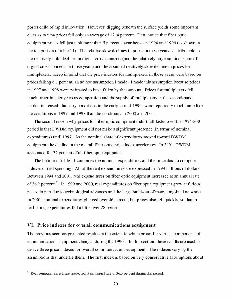
poster child of rapid innovation. However, digging beneath the surface yields some important

clues as to why prices fell only an average of 12 .4 percent. First, notice that fiber optic

equipment prices fell just a bit more than 5 percent a year between 1994 and 1996 (as shown in

the top portion of table 11). The relative slow declines in prices in these years is attributable to

the relatively mild declines in digital cross connects (and the relatively large nominal share of

digital cross connects in those years) and the assumed relatively slow decline in prices for

multiplexers. Keep in mind that the price indexes for multiplexers in those years were based on

prices falling 6.1 percent, an ad hoc assumption I made. I made this assumption because prices

in 1997 and 1998 were estimated to have fallen by that amount. Prices for multiplexers fell

much faster in later years as competition and the supply of multiplexers in the second-hand

market increased. Industry conditions in the early to mid-1990s were reportedly much more like

the conditions in 1997 and 1998 than the conditions in 2000 and 2001.

The second reason why prices for fiber optic equipment didn’t fall faster over the 1994-2001

period is that DWDM equipment did not make a significant presence (in terms of nominal

expenditures) until 1997. As the nominal share of expenditures moved toward DWDM

equipment, the decline in the overall fiber optic price index accelerates. In 2001, DWDM

accounted for 37 percent of all fiber optic equipment.

The bottom of table 11 combines the nominal expenditures and the price data to compute

indexes of real spending. All of the real expenditures are expressed in 1998 millions of dollars.

Between 1994 and 2001, real expenditures on fiber optic equipment increased at an annual rate

of 36.2 percent.21 In 1999 and 2000, real expenditures on fiber optic equipment grew at furious

paces, in part due to technological advances and the large build-out of many long-haul networks.

In 2001, nominal expenditures plunged over 46 percent, but prices also fell quickly, so that in

real terms, expenditures fell a little over 28 percent.

VI. Price indexes for overall communications equipment The previous sections presented results on the extent to which prices for various components of

communications equipment changed during the 1990s. In this section, those results are used to

derive three price indexes for overall communications equipment. The indexes vary by the

assumptions that underlie them. The first index is based on very conservative assumptions about

21 Real computer investment increased at an annual rate of 36.5 percent during this period.

20

price changes and the third index is based on aggressive assumptions about price changes.

Hopefully, the “truth” lies somewhere in between the two extreme cases. Like in the previous

sections, there are a fair number of tables with a large number of numbers. The three indexes are

located on the bottom of tables 14, 15, and 16.

Aggregate spending and production

Accurate spending figures are needed to derive aggregate deflators for communications

equipment. Table 12 summarizes spending and production of communications equipment. The

top panel of numbers in table 12 is from table 3, spending on communications equipment for

certain categories I obtained largely independent of government sources. The second panel of

numbers in table 12 shows the official numbers on communications equipment spending.22

Using the E&S, government, and consumer spending figures, total domestic spending on

communications equipment grew at an average rate of 14.2 percent between 1997 and 2000, only

½ percentage point faster than the figures from table 3.

Another point to note is the difference in the magnitude of the spending figures in table 3

(line 1) and line 10--the official domestic spending figures are 30 to 40 percent higher than those

in table 3. One reason why the domestic spending figures are larger than those in table 3 is that

the domestic spending figures include additional items, such as radio equipment (outside of

cellular phone equipment), broadcast and studio equipment, and alarm systems.

The bottom portion of table 3 shows estimates of production of communications equipment,

a concept similar to the GDP figures in line 4. Surprisingly, industry shipments and product

shipments increased at faster rates than the GDP figures. Why this is the case is unclear.

Overall, the point to take away from table 12 is that several independent sources concur that

domestic spending on communications equipment increased at a fairly rapid clip in the late

1990s and that production of communications equipment also increased quickly. Further, the

spending estimates from table 3 account for a majority of all communications equipment

spending.

22 The government and consumer spending figures are not published on a regular basis, and, in fact, were last published for 1992. The government expenditure figures were extrapolated to 2000 by assuming the growth rate was half that of the E&S series. The consumer spending numbers are based on those I derived in table 3 and on the 1992 input-output tables. Private-sector spending on communications gear likely grew much faster than government spending during the 1990s. As a result of The Telecommunications Act of 1996, a flood of entrants entered into the telecommunication service industry. Also, as stated previously, there was a surge in spending on fiber optic equipment that was tied to the build-out of long-haul fiber networks. These networks are private.

21

Constructing overall communications equipment price indexes

I employ a bottom-up approach to construct overall price indexes for communications

equipment--the estimates of price indexes for various components of communications equipment

are chain weighted. The assumptions made about prices for the conservative, moderate, and

aggressive scenarios are displayed in table 13. Tables 14 through 16 show the results based on

these assumptions. Table 17 shows a summary of the three sets of results.

Conservative assumptions. Lines 1 through 6 in the top portion of table 14 show the price

indexes used in place of the PPI for a select group of products. For the conservative

assumptions, only those price indexes are used that were discussed earlier in this paper. That set

of results includes previous results on cell phones, central office switching equipment, and LAN

equipment. Added to these three sets of results are those that are developed in this paper--fiber

optic equipment, PBXs, and modems. For all other communications equipment, the conservative

approach uses the PPI for communications equipment.23

These price indexes in lines 1 through 6 are chain-weighted using the weights in lines 7

through 12. The aggregate price index for these products, line 15, fall an average of 15.0 percent

between 1994 and 2000, with the fastest price declines occurring in the later three years. In

contrast, the overall PPI for communications equipment (line 19) falls at a 0.4 percent annual

rate.

The price index for the special products does not include the prices for products not listed in

lines 1 through 6. The conservative approach assumes that prices for all other communications

equipment follow the PPI. Line 22 shows the overall price index for communications equipment

under the conservative assumptions--prices fall an average of 6.4 percent, 6 percentage points

faster than the PPI and 6-1/2 percentage points faster than BEA’s communications equipment

price index (line 24). Recall that the BEA index already makes an adjustment for two of the six

product categories in lines 1 through 6--LAN equipment and central office switching and

transmission equipment.

23 Ideally each product would be linked to its own PPI. However, I found that a concordance between my system and the SIC was difficult to construct. Also, most PPIs within SIC 366 do not show much change over the late 1990s, so even if I were to use a more refined concordance, the overall results would not change very much.

22

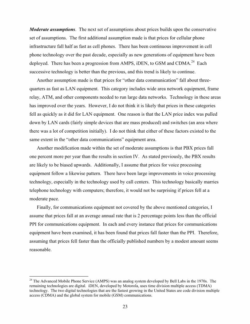
Moderate assumptions. The next set of assumptions about prices builds upon the conservative

set of assumptions. The first additional assumption made is that prices for cellular phone

infrastructure fall half as fast as cell phones. There has been continuous improvement in cell

phone technology over the past decade, especially as new generations of equipment have been

deployed. There has been a progression from AMPS, iDEN, to GSM and CDMA.24 Each

successive technology is better than the previous, and this trend is likely to continue.

Another assumption made is that prices for “other data communication” fall about three-

quarters as fast as LAN equipment. This category includes wide area network equipment, frame

relay, ATM, and other components needed to run large data networks. Technology in these areas

has improved over the years. However, I do not think it is likely that prices in these categories

fell as quickly as it did for LAN equipment. One reason is that the LAN price index was pulled

down by LAN cards (fairly simple devices that are mass produced) and switches (an area where

there was a lot of competition initially). I do not think that either of these factors existed to the

same extent in the “other data communications” equipment area.

Another modification made within the set of moderate assumptions is that PBX prices fall

one percent more per year than the results in section IV. As stated previously, the PBX results

are likely to be biased upwards. Additionally, I assume that prices for voice processing

equipment follow a likewise pattern. There have been large improvements in voice processing

technology, especially in the technology used by call centers. This technology basically marries

telephone technology with computers; therefore, it would not be surprising if prices fell at a

moderate pace.

Finally, for communications equipment not covered by the above mentioned categories, I

assume that prices fall at an average annual rate that is 2 percentage points less than the official

PPI for communications equipment. In each and every instance that prices for communications

equipment have been examined, it has been found that prices fall faster than the PPI. Therefore,

assuming that prices fell faster than the officially published numbers by a modest amount seems

reasonable.

24 The Advanced Mobile Phone Service (AMPS) was an analog system developed by Bell Labs in the 1970s. The remaining technologies are digital. iDEN, developed by Motorola, uses time division multiple access (TDMA) technology. The two digital technologies that are the fastest growing in the United States are code division multiple access (CDMA) and the global system for mobile (GSM) communications.

23

Under these assumptions, prices for communications equipment fell at an 8.3 percent annual

rate, more than one-third as fast as the BEA computer price index and over 5 percentage points

faster than the BEA communications equipment price index.

Aggressive assumptions. Finally, table 16 presents results under the aggressive assumptions.

The aggressive assumptions are laid out in table 13. The biggest difference between the

aggressive and moderate assumptions is that the PPI is assumed to fall 4 percentage points faster

than the official PPI--under the moderate assumptions, the PPI was assumed to fall 2 percentage

points faster than the official series.

Under the aggressive assumptions, prices for communications equipment fall at a 10.6

percent annual rate, about two percentage points faster than the moderate assumptions.

VII. Investment and MFP In this section we address the implications of the mismeasurement of communications equipment

prices. Specifically, we examine how growth rates in various investment aggregates would

change if the alternative price indexes for communications equipment are used. The calculations

are performed for investment in communications equipment, information processing equipment,

and for total nonresidential investment. One reason why we might be interested in how the

growth rates of real investment change as a result of new deflators is that it may alter the results

on capital deepening and multi-factor productivity (MFP). Later in this section we address this

issue.

Basically, the real growth rates of various investment categories will increase as a result of

using the price indexes in the previous section. What influences the effect of new

communications equipment deflators on various aggregates is the nominal share of

communications equipment of the aggregates. Roughly speaking, the effect of altering the price

index for communications equipment is proportional to the nominal share of communications

equipment. Between 1994 and 2000, communications equipment made up approximately 1/4

percent of all investment in information processing equipment and software and 10 percent of all

nonresidential investment.

How the growth rates for real communications equipment, information processing

equipment, and total non-residential investment are affected by the conservative, moderate, and

aggressive price indexes are displayed in table 18. The figures in table 18 reflect how much the

24

average growth rate for those series would increase under the various assumptions about

communications equipment pricing.

As shown in the bottom left of the table, if the aggressive deflators are used, then the average

annual growth rate for real investment in communications equipment increases by 9.8 percentage

points between 1994 and 2000. The effects of the aggressive deflator on information processing

equipment and on non-residential investment are smaller, but still considerable. Even if the

conservative deflator is used, real non-residential investment would be boosted by 0.4 percentage

point per year.

The results in table 18 are averages over 1994 and 2000. Figure 7 shows the data on an

annual basis for non residential investment. Each of the lines corresponds to one of the three

assumptions about communications equipment prices. As shown, the changes to the deflators

have the largest effects for 1997-2000, the period in which nominal spending on fiber optic

equipment grew rapidly. In a nutshell, adopting deflators for communications equipment that

more likely reflect actual price movements would have non trivial effects on a variety of

investment categories.

One reason why the growth rate in real investment is of interest is because of the relationship

between real investment, the capital stock, and productivity. This is especially true of the

acceleration of productivity in the second half of the 1990s when current estimates suggest that

there was a significant contribution from capital deepening and a significant contribution from

acceleration in MFP.

One way in which the changes in the growth rate of communications equipment feeds into

changes in productivity is the output effect; the growth rate of overall output is increased because

of the growth rate of one of the parts has increased. The output effect is small given the small

share of communications equipment to total output; the average share of communications

equipment to total GDP between 1994 and 2000 is about 0.9 percent, and about 1.1 percent of

total non-farm business output. Even if the aggressive results are used, GDP growth would be

boosted by less than 0.1 percent per year.

The other way in which the deflators affect productivity is through the contribution to the

growth rate of capital services; a higher growth rate in capital services will shift some of the

increase from multi factor productivity growth towards capital deepening. One way to estimate

the effect changes in capital deepening is by examining the product of the capital income share

of communications equipment and the change in the real growth rate in communications

25

equipment. Daniel Sichel has estimated that the communication equipment share during the later

half of the 1990s is a bit less than 2 percent. The moderate deflators for communications

equipment would boost real communications equipment growth by an average of 6-1/2 percent,

resulting in capital deepening increasing by a bit more than 0.1 percentage point per year. To put

this result in some context, between 1997 and 2000, Daniel Sichel estimates that MFP grew at a

1.1 percent average rate; the moderate results in this paper on communications equipment would

likely lower that estimate to closer to 1.0 percent. If the more aggressive assumptions about

communications equipment prices were used, then MFP growth would be lowered to closer 0.9

percent per year.

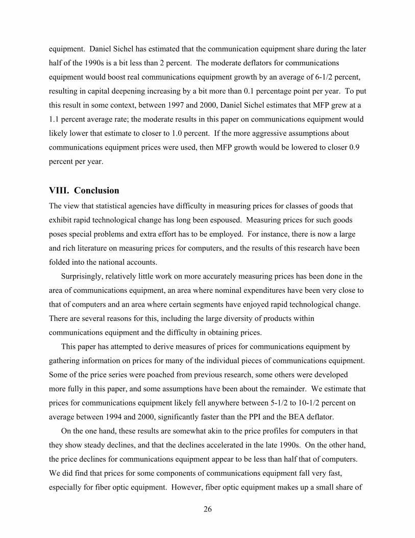
VIII. Conclusion The view that statistical agencies have difficulty in measuring prices for classes of goods that

exhibit rapid technological change has long been espoused. Measuring prices for such goods

poses special problems and extra effort has to be employed. For instance, there is now a large

and rich literature on measuring prices for computers, and the results of this research have been

folded into the national accounts.

Surprisingly, relatively little work on more accurately measuring prices has been done in the

area of communications equipment, an area where nominal expenditures have been very close to

that of computers and an area where certain segments have enjoyed rapid technological change.

There are several reasons for this, including the large diversity of products within

communications equipment and the difficulty in obtaining prices.

This paper has attempted to derive measures of prices for communications equipment by

gathering information on prices for many of the individual pieces of communications equipment.

Some of the price series were poached from previous research, some others were developed

more fully in this paper, and some assumptions have been about the remainder. We estimate that

prices for communications equipment likely fell anywhere between 5-1/2 to 10-1/2 percent on

average between 1994 and 2000, significantly faster than the PPI and the BEA deflator.

On the one hand, these results are somewhat akin to the price profiles for computers in that

they show steady declines, and that the declines accelerated in the late 1990s. On the other hand,

the price declines for communications equipment appear to be less than half that of computers.

We did find that prices for some components of communications equipment fall very fast,

especially for fiber optic equipment. However, fiber optic equipment makes up a small share of

26

total communications equipment, and so the influence it has on the larger communications

aggregate is muted.

Our results are also roughly consistent with several independent sources of information on

technological change and price declines. First, Aizcorbe, Flamm, and Khurshid find that the

prices for semiconductors that go into communications equipment do not fall as quickly as prices

of chips that go into computers. Further, semiconductor content in computers is higher. Second,

figure 2 showed that the number of patents awarded to communications equipment was much

less than those awarded for computers in the late 1990s.

One can speculate for other reasons why prices for communications equipment do not fall as

quickly as computers may because the communications equipment industry is much more

fragmented than that for computer hardware. Achieving economies of scale or proceeding up

learning curves as are important for computers and semiconductors does not appear to happen

often within communications equipment, with the exception of cell phones and LAN cards.

The implications for the results in this paper are that real investment in certain categories was

much higher than actually reported. For instance, real nonresidential investment would be from

0.5 to 1.0 percentage point higher between 1997 and 2000 if the deflators presented in this paper

were used. This higher rate of real investment also feeds into higher rates of capital

accumulation, resulting in shifting a small portion of the growth in MFP in the late 1990s to

capital deepening.

27

28

References Aizcorbe. A., C. Corrado, and M. Doms (2003) “When Do Mathced-Model and Hedonic Techniques Yield Similar Price Measures,” Working Paper, Federal Reserve Bank of San Francisco. Aizcorbe, A., K. Flamm, and A. Khurshid (2002) “The Role of Semiconductor Inputs in IT Hardware Price Decline: Computers vs. Communications, “ FEDS Working Paper 2002-37. Doms, Mark and Christopher Forman (2003), “Price for LAN Equipment,” San Francisco Federal Reserve Working Paper #___. Flamm, Kenneth (1989) “Technological Advance and Costs: Computers versus Communications” in Robert Crandall and Kenneth Flamm, eds. Changing the Rules: Technological Change, International Competition, and Regulation in Communications. Washington: The Brookings Institution. 13-61. Forman, C. and M. Doms (1999) “Price Declines and Consumer Welfare Benefits in Computer Networking Equipment,” Working Paper, Kellogg School of Management, Northwestern University. Gordon, Robert J. (1990). The Measurement of Durable Goods Prices. National Bureau of Economic Research Monograph. Grimm, Bruce (1996) “A Quality Adjusted Price Index for Digital Telephone Switches,” Working Paper, Burea of Economic Analysis. Jorgenson, Dale and Kevin Stiroh (2000), “Raising the Speed Limit: U.S. Economic Growth in the Information Age”, Brookings Papers on Economic Activity, v.0, pp. 125-211. Shapiro, M. and D. Wilcox (1996) “Mismeasurement in the Consumer Price Index: An Evaluation,” in B.S. Bernanke and J.J. Rotemberg, eds. NBER Macroeconomics Annual. Cambridge, MA: MIT Press. Telecommunications Industry Association. Multimedia Telecommunications Market Review and Forecast, various years. Trajtenberg, M. (1989) Economic Analysis of Product Innovation: The Case of CT Scanners. Cambridge, Massachusetts: Harvard University Press. Triplett, J. (1989) Price and Technical Change in a Capital Good: A Survey of Research on Computers. in D. Jorgenson and R. Landau, eds. Technology and Capital Formation. Cambridge, MA: MIT Press. 127-213.

Initial transmission

Home phone

Cell phonePDA

Business phone

Voice

Computer (LAN card, modem)

Data

Home phone

Cell phonePDA

Business phone

Computer (LAN card, modem)

Terminus

Switching*center

SwitchingcenterCell

phone tower

LAN WAN

Cable TVnetwork

PBX/KTS

Cable TVnetwork

LAN

PBX/KTS

Cell Phone tower-Microwave

-Fiber-Satellite-Copper

Figure 1 . A simplified version of voice and data communication networks

*Equipment in switching centers contain gear that accepts incoming information from many different languages, protocols, and mediums and then decides where to send the information next. This gear includes voice switches and fiber optic equipment.LAN - local area network. PBX = public branch exchange.WAN - wide area network. KTS = keystone telephone system.PDA - personal digital assistant.

Figure 2. Share of U.S. patents by high-technology category

0

2

4

6

8

10

12

14

16

1963 1967 1971 1975 1979 1983 1987 1991 1995 1999

Year

Sh

are

of

U.S

. pat

ents

(p

erce

nt)

Communicationsequipment

Semiconductors

Computers andperipherals

Source: Manuel TrajtenbergComputers and peripherals=computer hardware and software + computer peripherals + information storage.

Figure 3: Price Indices For Modems

1.00

1.20

1.40

1.60

1.80

2.00

89Q1

89Q3

90Q1

90Q3

91Q1

91Q3

92Q1

92Q3

93Q1

93Q3

94Q1

94Q3

95Q1

95Q3

96Q1

96Q3

97Q1

97Q3

98Q1

98Q3

99Q1

99Q3

00Q1

00Q3

01Q4

Date

Ind

ex (L

og

Sca

le)

All analog (89Q1) 14400 (92Q3)

28800 (94Q4) 36600 (96Q1)

56000 (97Q2) Cable (99Q4)

BEA E&S Computer Price Index (89Q1) 1200 (89Q1)

2400 (98Q1) 9600 (91Q4)

Source: Analog modem data were collected from CDW and ACP advertisements in PC World magazine beginning February, 1989 (Q1). The 681 observations were generally U.S. Robotics, Hayes, and Practical Peripheral models. Cable modem figures (1999Q4 to 2001Q4) were derived from market statistics produced by Gartner, Inc. Computer and communications equipment price data are from BEA.

Average Annual Growth Rate:(89Q1 to 98Q3)

Analog modems: -15.93BEA E&S Computer Price Index: -17.10

100

80

60

40

20

10

Figure 4: Price Indices For Modems over 10K bps

1.48

1.58

1.68

1.78

1.88

1.98

92Q2

92Q4

93Q2

93Q4

94Q2

94Q4

95Q2

95Q4

96Q2

96Q4

97Q2

97Q4

98Q2

98Q4

99Q2

99Q4

00Q2

00Q4

Date

Ind

ex (L

og

Sca

le)

14400 (92Q3) 28800 (94Q4)

36600 (96Q1) 56000 (97Q2)

BLS Modems > 10K (94Q2) FRB Index for Modems > 10K

Source: Analog modem data were collected from CDW and ACP advertisements in PC World magazine beginning February, 1989 (Q1). The 681 observations were generally U.S. Robotics, Hayes, and Practical Peripheral models. Cable modem figures (1999Q4 to 2001Q4) were derived from market statistics produced by Gartner, Inc. Computer and communications equipment price data are from BEA.

Average Annual Growth Rate:(94Q2 to 98Q3)

FRB Index for Modems > 10K: -15.43

BLS Modems > 10K: -8.65

100

80

60

40

30

Figure 5: Alexander Graham Bell’s Photophone

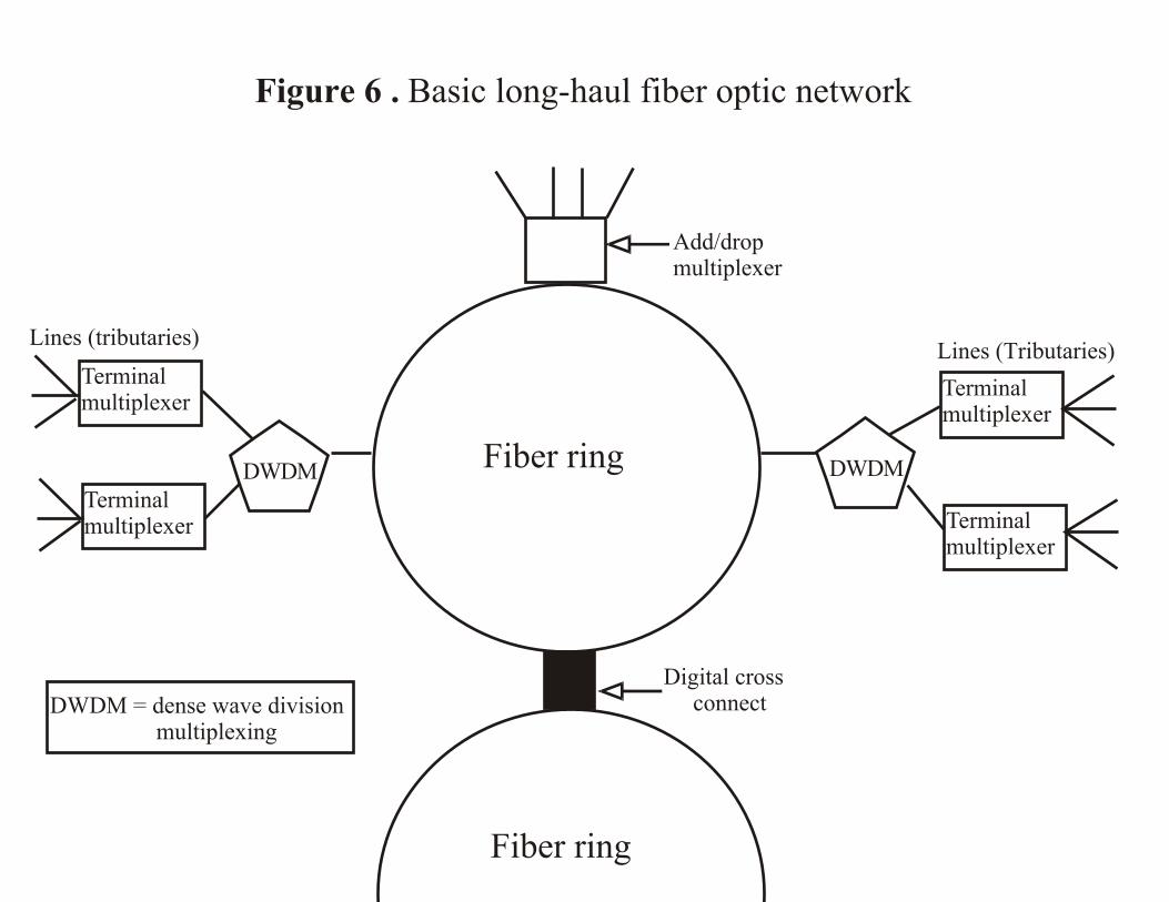
DWDM

Terminal multiplexer

Lines (tributaries)

Fiber ring DWDM

Add/drop multiplexer

Digital cross connect

Fiber ring

Figure 6 . Basic long-haul fiber optic network

Lines (Tributaries)

Terminal multiplexer Terminal

multiplexer

Terminal multiplexer

DWDM = dense wave division multiplexing

Figure 7: Changes in the real growth rate in non-residential investment under differing assumptions for communications equipment prices

-0.20

0.00

0.20

0.40

0.60

0.80

1.00

1.20

1995 1996 1997 1998 1999 2000

AggressiveModerateConservative

Average nominal growth in investment (%)1. 1990-1995 5.6 5.02. 1995-2000 10.6 10.53. 1990-2000 8.0 7.6

4. Level of investment, 2000 ($billions) 109.3 116.8

Average annual price change (%)5. 1990-1995 -12.6 -1.16. 1995-2000 -21.6 -2.97. 1990-2000 -17.6 -2.1

Average real growth rates (%)8. 1990-1995 20.9 6.29. 1995-2000 41.0 13.8

10. 1990-2000 31.1 9.9

ComputersCommunications

Equipment

Table 1: Business Investment in Computers and Communications Equipment

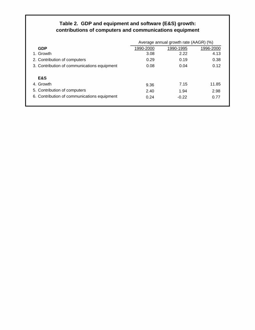
GDP 1990-2000 1990-1995 1996-20001. Growth 3.08 2.22 4.132. Contribution of computers 0.29 0.19 0.383. Contribution of communications equipment 0.08 0.04 0.12

E&S 4. Growth 9.36 7.15 11.855. Contribution of computers 2.40 1.94 2.986. Contribution of communications equipment 0.24 -0.22 0.77

contributions of computers and communications equipment

Average annual growth rate (AAGR) (%)

Table 2. GDP and equipment and software (E&S) growth:

1997 1998 1999 2000 AAGR (%)Switching center equipment (1) 27,055 29,577 36,870 46,548 19.8

Central office switching and transmission equipment 12,358 13,562 14,475 15,500 7.8Fiber optic equipment 7,160 9,059 14,081 22,061 45.5Cellular phone infrastructure 5,678 4,474 4,955 4,734 -5.9

Data communication (2) 24,134 27,745 30,306 33,870 12.0

LAN Equipment 11,437 13,111 14,027 15,838 11.5Routers 2,986 3,425 4,525 5,946 25.8LAN switches 3,787 5,706 6,528 7,645 26.4Hubs 1,884 1,538 761 419 -39.4LAN Cards 2,780 2,442 2,213 1,829 -13.0

Modems 3,077 3,290 2,800 2,500 -6.7Other (WAN, ISDN, ATM, Frame relay, et cetera) 9,620 11,344 13,479 15,532 17.3

Voice equipment (3) 22,855 25,172 26,424 27,437 6.3Business phone equipment 11,795 13,227 14,195 15,135 8.7

Private Branch Exchange (PBX)/Key Telephone System (KTS) 6,832 7,601 7,980 8,392 7.1Voice processing equipment (call centers, voice mail, et cetera) 4,963 5,626 6,215 6,743 10.8

Wireless handsets (cell phones) 5,787 7,228 7,619 7,692 10.0 Consumer products 5,273 4,717 4,610 4,610 -4.4

Cordless telephones 2,099 2,250 2,240 2,260 2.5Answering machines 1,173 1,240 1,215 1,210 1.0Home fax machines 1,367 655 625 620 -23.2Corded telephones 634 572 530 520 -6.4

Other (4) 3,400 3,850 5,400 6,000 20.8 Capital equipment spending by cable television firms not covered above 3,400 3,850 5,400 6,000 20.8

Total Spending (1) + (2) + (3) + (4) 77,444 86,344 99,000 113,855 13.7

Consumer products 8,167 8,331 8,420 8,456 1.2Total Spending - Consumer Products 69,277 78,013 90,581 105,399 15.0

PDE Communications Equipment 73,739 81,236 93,350 116,837 16.6Source: Dataquest, FCC, TIA, RHK, KMI, Author's Estimates

Table 3: Spending on Telecommunications Equipment ($millions)

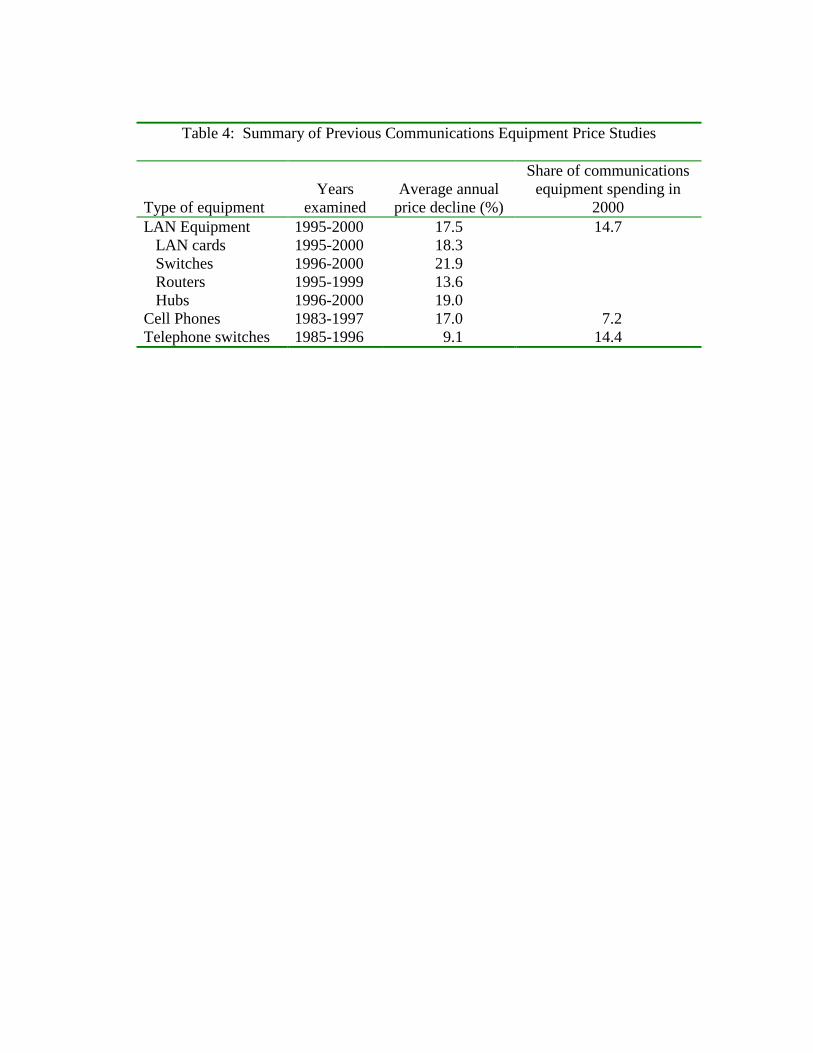
Table 4: Summary of Previous Communications Equipment Price Studies

Type of equipment

Years

examined

Average annual

price decline (%)

Share of communications equipment spending in

2000 LAN Equipment 1995-2000 17.5 14.7 LAN cards 1995-2000 18.3 Switches 1996-2000 21.9 Routers 1995-1999 13.6 Hubs 1996-2000 19.0 Cell Phones 1983-1997 17.0 7.2 Telephone switches 1985-1996 9.1 14.4

1 to 8 9 to 24 24 to 48 49 to 100 101 to 400 401 to 1000 Price Index

1994 Price 2,701 6,856 17,226 47,806 170,511 589,428 1.00

Quantity 190,000 99,200 50,400 27,400 5,400 1,100

Revenue ($millions) 513 680 868 1,310 921 648

1995 Price 2,851 7,231 18,465 50,057 169,567 567,416 1.03

Quantity 199,200 100,600 47,200 24,600 6,300 1,200

Revenue 568 727 872 1,231 1,068 681

1996 Price 2,374 6,819 18,406 44,295 166,433 530,018 0.96

Quantity 187,814 117,311 46,759 26,863 6,982 1,298

Revenue 446 800 861 1,190 1,162 688

1997 Price 1,900 6,953 17,851 43,054 148,222 498,172 0.90

Quantity 283,544 122,099 50,570 34,798 8,366 1,553

Revenue 539 849 903 1,498 1,240 774

1998 Price 1,732 7,253 17,799 40,319 139,287 435,616 0.86

Quantity 289,765 113,446 52,744 39,974 10,696 1,769

Revenue 502 823 939 1,612 1,490 771

1999 Price 1,733 6,622 16,138 38,462 122,320 413,277 0.79

Quantity 233,233 124,369 63,167 44,283 13,898 1,842

Revenue 404 824 1,019 1,703 1,700 761

2000 Price 1,996 6,424 15,550 36,393 103,316 408,678 0.75

Quantity 228,883 96,716 57,085 36,215 15,734 1,692

Revenue 457 621 888 1,318 1,626 691

AAGR (%) -4.9 -1.1 -1.7 -4.4 -8.0 -5.9 -4.8

Table 5: Average Prices and Quantities for PBX Systems by Number of Lines

Number of lines

Sources: U.S. Premise Switching Systems Market Share and Forecast, 2000: Market Statistics, Gartner Group, Inc May 8, 2000, U.S. Premise Switching Systems Market Share and Forecast, 1999: Market Statistics, Gartner Group, Inc. April 12, 1999, and U.S. PBX/KTS and PCX Market Share and Forecast, 2001: Market Statistics Gartner Group, Inc. May 31, 2001.

Table 6: Fiber Optic Glossary

Multiplexer (also known as a “mux”). Devices that can input multiple signals to produce a single signal, and devices that input a single signal and produce multiple signals. An add/drop mux selectively adds and/or drops wavelengths without having to use terminal equipment. A teminal mux extracts all signals/wavelengths from the fiber. Dense wave division multiplexing (DWDM), also known as wavelength division multiplexing. Equipment that transmits multiple lightwaves down a single piece of fiber. For instance, there are DWDM devices that can send and receive 40 different wavelengths, with each wavelength having a maximum capacity of 2.5 gigabytes per second. A DWDM system of this type could send 100 gigabytes per second. Digital cross connect, a device that is able perform simple extraction and merging onto a fiber ring. Regenerator, a device that takes an attenuated optical signal and re-issues the signal in a “cleaner” form.

1994 1995 1996 1997 1998 1999 2000 2001 AAGR (%)Total Fiber Optic Equipment 3,443 4,163 5,112 7,160 9,059 14,081 22,061 11,842 19.3(percent change) 20.9 22.8 40.0 26.5 55.4 56.7 -46.3

Multiplexers 1,865 2,406 2,656 3,562 4,556 7,291 10,573 4,880.0 14.7Dense Wavelength Division Multiplexing (DWDM) 0 0 381 1,595 1,854 3,427 6,740 4,348 62.7Digital Cross Connects 1,111 1,182 1,455 1,581 2,210 2,749 3,950 1,914.0 8.1Other 467 576 620 422 439 614 799 700 5.9

Source: RHK, Gartner, KMI.

Table 7: Nominal Spending of Fiber Optic Equipment ($ millions)

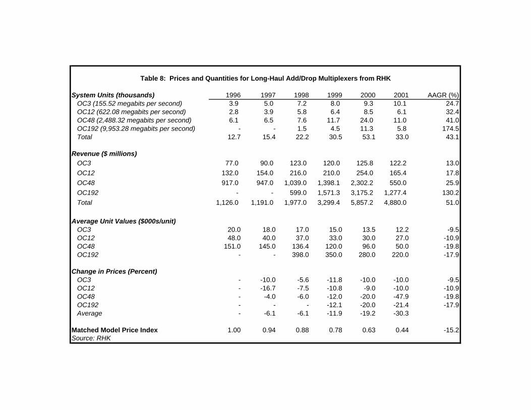
System Units (thousands) 1996 1997 1998 1999 2000 2001 AAGR (%)OC3 (155.52 megabits per second) 3.9 5.0 7.2 8.0 9.3 10.1 24.7OC12 (622.08 megabits per second) 2.8 3.9 5.8 6.4 8.5 6.1 32.4OC48 (2,488.32 megabits per second) 6.1 6.5 7.6 11.7 24.0 11.0 41.0OC192 (9,953.28 megabits per second) - - 1.5 4.5 11.3 5.8 174.5Total 12.7 15.4 22.2 30.5 53.1 33.0 43.1

Revenue ($ millions)OC3 77.0 90.0 123.0 120.0 125.8 122.2 13.0OC12 132.0 154.0 216.0 210.0 254.0 165.4 17.8OC48 917.0 947.0 1,039.0 1,398.1 2,302.2 550.0 25.9OC192 - - 599.0 1,571.3 3,175.2 1,277.4 130.2Total 1,126.0 1,191.0 1,977.0 3,299.4 5,857.2 4,880.0 51.0

Average Unit Values ($000s/unit)OC3 20.0 18.0 17.0 15.0 13.5 12.2 -9.5OC12 48.0 40.0 37.0 33.0 30.0 27.0 -10.9OC48 151.0 145.0 136.4 120.0 96.0 50.0 -19.8OC192 - - 398.0 350.0 280.0 220.0 -17.9

Change in Prices (Percent)OC3 - -10.0 -5.6 -11.8 -10.0 -10.0 -9.5OC12 - -16.7 -7.5 -10.8 -9.0 -10.0 -10.9OC48 - -4.0 -6.0 -12.0 -20.0 -47.9 -19.8OC192 - - - -12.1 -20.0 -21.4 -17.9Average - -6.1 -6.1 -11.9 -19.2 -30.3

Matched Model Price Index 1.00 0.94 0.88 0.78 0.63 0.44 -15.2Source: RHK

Table 8: Prices and Quantities for Long-Haul Add/Drop Multiplexers from RHK

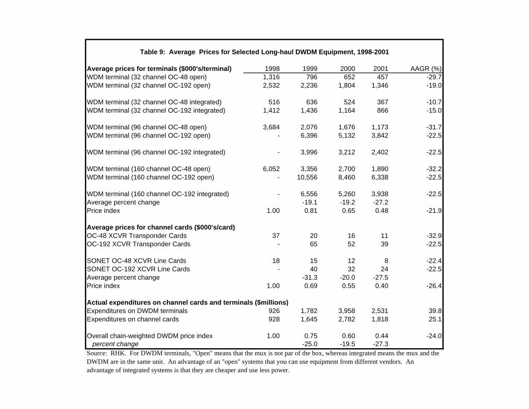
Average prices for terminals ($000's/terminal) 1998 1999 2000 2001 AAGR (%)WDM terminal (32 channel OC-48 open) 1,316 796 652 457 -29.7WDM terminal (32 channel OC-192 open) 2,532 2,236 1,804 1,346 -19.0

WDM terminal (32 channel OC-48 integrated) 516 636 524 367 -10.7WDM terminal (32 channel OC-192 integrated) 1,412 1,436 1,164 866 -15.0

WDM terminal (96 channel OC-48 open) 3,684 2,076 1,676 1,173 -31.7WDM terminal (96 channel OC-192 open) - 6,396 5,132 3,842 -22.5

WDM terminal (96 channel OC-192 integrated) - 3,996 3,212 2,402 -22.5

WDM terminal (160 channel OC-48 open) 6,052 3,356 2,700 1,890 -32.2WDM terminal (160 channel OC-192 open) - 10,556 8,460 6,338 -22.5

WDM terminal (160 channel OC-192 integrated) - 6,556 5,260 3,938 -22.5Average percent change -19.1 -19.2 -27.2Price index 1.00 0.81 0.65 0.48 -21.9 Average prices for channel cards ($000's/card)OC-48 XCVR Transponder Cards 37 20 16 11 -32.9OC-192 XCVR Transponder Cards - 65 52 39 -22.5

SONET OC-48 XCVR Line Cards 18 15 12 8 -22.4SONET OC-192 XCVR Line Cards - 40 32 24 -22.5Average percent change -31.3 -20.0 -27.5Price index 1.00 0.69 0.55 0.40 -26.4

Actual expenditures on channel cards and terminals ($millions)Expenditures on DWDM terminals 926 1,782 3,958 2,531 39.8Expenditures on channel cards 928 1,645 2,782 1,818 25.1

Overall chain-weighted DWDM price index 1.00 0.75 0.60 0.44 -24.0percent change -25.0 -19.5 -27.3

Table 9: Average Prices for Selected Long-haul DWDM Equipment, 1998-2001

Source: RHK. For DWDM terminals, "Open" means that the mux is not par of the box, whereas integrated means the mux and the DWDM are in the same unit. An advantage of an "open" systems that you can use equipment from different vendors. An advantage of integrated systems is that they are cheaper and use less power.

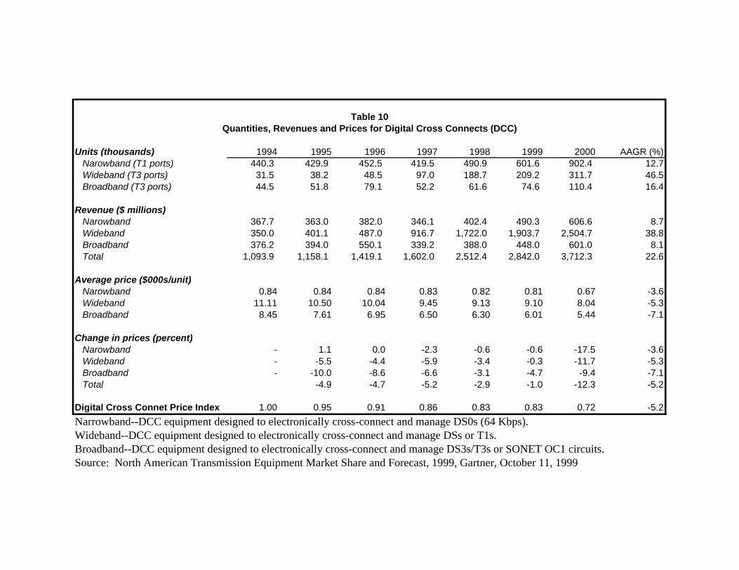
Units (thousands) 1994 1995 1996 1997 1998 1999 2000 AAGR (%)Narowband (T1 ports) 440.3 429.9 452.5 419.5 490.9 601.6 902.4 12.7Wideband (T3 ports) 31.5 38.2 48.5 97.0 188.7 209.2 311.7 46.5Broadband (T3 ports) 44.5 51.8 79.1 52.2 61.6 74.6 110.4 16.4

Revenue ($ millions)Narowband 367.7 363.0 382.0 346.1 402.4 490.3 606.6 8.7Wideband 350.0 401.1 487.0 916.7 1,722.0 1,903.7 2,504.7 38.8Broadband 376.2 394.0 550.1 339.2 388.0 448.0 601.0 8.1Total 1,093.9 1,158.1 1,419.1 1,602.0 2,512.4 2,842.0 3,712.3 22.6

Average price ($000s/unit)Narowband 0.84 0.84 0.84 0.83 0.82 0.81 0.67 -3.6Wideband 11.11 10.50 10.04 9.45 9.13 9.10 8.04 -5.3Broadband 8.45 7.61 6.95 6.50 6.30 6.01 5.44 -7.1

Change in prices (percent)Narowband - 1.1 0.0 -2.3 -0.6 -0.6 -17.5 -3.6Wideband - -5.5 -4.4 -5.9 -3.4 -0.3 -11.7 -5.3Broadband - -10.0 -8.6 -6.6 -3.1 -4.7 -9.4 -7.1Total -4.9 -4.7 -5.2 -2.9 -1.0 -12.3 -5.2

Digital Cross Connet Price Index 1.00 0.95 0.91 0.86 0.83 0.83 0.72 -5.2

Source: North American Transmission Equipment Market Share and Forecast, 1999, Gartner, October 11, 1999

Table 10Quantities, Revenues and Prices for Digital Cross Connects (DCC)

Narrowband--DCC equipment designed to electronically cross-connect and manage DS0s (64 Kbps). Wideband--DCC equipment designed to electronically cross-connect and manage DSs or T1s.Broadband--DCC equipment designed to electronically cross-connect and manage DS3s/T3s or SONET OC1 circuits.

Price Indexes (1998=1.0) 1994 1995 1996 1997 1998 1999 2000 2001 AAGR (%)Total Fiber Optic Equipment 1.36 1.28 1.21 1.10 1.00 0.87 0.72 0.54 -12.4(percent change) -5.7 -5.3 -9.0 -9.3 -12.6 -17.9 -25.2

Multiplexers 1.29 1.21 1.13 1.07 1.00 0.88 0.71 0.50 -12.7Dense Wavelength Division Multiplexing (DWDM) 1.73 1.32 1.00 0.75 0.60 0.44 -17.8Digital Cross Connects 1.20 1.14 1.09 1.03 1.00 0.99 0.87 0.80 -5.6

Nominal Spending ($millions)Total Fiber Optic Equipment 3,443 4,163 5,112 7,160 9,059 14,081 22,061 11,842 19.3(percent change) 20.9 22.8 40.0 26.5 55.4 56.7 -46.3

Multiplexers 1,865 2,406 2,656 3,562 4,556 7,291 10,573 4,880 14.7Dense Wavelength Division Multiplexing (DWDM) 0 0 381 1,595 1,854 3,427 6,740 4,348 41.6Digital Cross Connects 1,111 1,182 1,455 1,581 2,210 2,749 3,950 1,914 8.1

Real Spending (1998 $millions)Total Fiber Optic Equipment 2,536 3,251 4,217 6,491 9,059 16,112 30,762 22,089 36.2(percent change) 28.2 29.7 53.9 39.6 77.9 90.9 -28.2

Multiplexers 1,449 1,991 2,341 3,343 4,556 8,277 14,847 9,835 31.5Dense Wavelength Division Multiplexing (DWDM) 220 1,212 1,854 4,571 11,172 9,914 72.3Digital Cross Connects 928 1,037 1,340 1,535 2,210 2,777 4,550 2,396 14.5

Notes: It is assumed that prices for multiplexers fell an average of 6.1 percent in between 1994 and 1996, the same rate as was estimated for 1996 to 1998. The price index for DWDM equipment is assumed to fall 24 percent, the average rate from 1998 to 2001.The price index for digital cross connects in 2001 is assumed to fall 8.0 percent, a slightly faster rate than in previous years because of increased competition in the industry.

Table11: Summary Indexes for Fiber Optic Equipment

Categories from table 3 1994 1995 1996 1997 1998 1999 20001997-2000 AAGR (%)

1. Total 77,444 86,344 99,000 113,855 13.72. Consumer 8,167 8,331 8,420 8,456 1.23. Business and government spending 69,277 78,013 90,581 105,399 15.0

GDP accounting4. Communications equipment GDP (5+6+7+8-9) 69,598 77,401 83,740 97,461 103,176 110,710 124,249 8.45. E&S 54,743 60,019 65,609 73,700 81,200 93,300 116,800 16.66. Government 12,914 13,533 14,157 15,017 15,771 16,919 18,983 8.17. Consumer spending 4,523 4,958 5,420 8,167 8,331 8,420 8,456 1.28. Exports 11,237 13,762 14,469 17,683 18,209 20,008 23,284 9.69. Imports 13,819 14,871 15,915 17,105 20,335 27,937 43,274 36.3

Memo:10. Domestic spending (5+6+7) 72,180 78,510 85,186 96,883 105,302 118,639 144,239 14.211. (10-1) 27,606 27,289 28,058 38,839 12.1

ASM production information12. Industry shipments 48,052 58,499 68,232 82,852 86,119 97,953 119,329 12.913. ASM product shipments 48,440 55,431 63,968 78,142 81,932 92,715 107,921 11.4

Table 12: Communications Equipment, Spending and Production ($millions)

Equipment Type Conservative Moderate Aggressive CommentsCentral office switching and transmission equipment

BEA (16.1 percent decline per year)

BEA BEA

Fiber optic equipment section V results section V results section V results

Cellular phone infrastructure PPI -7.5 percent per year, half that of cellular phones

-10 percent per year, two-thrids that of cellular phones

There has been continuous improvement in cell phone technology over the past decade and there has been increased competition in the base station equipment market.

LAN Equipment Doms and Forman Doms and Forman Doms and Forman

Modems section IV results section IV results section IV results

Other data communications (WAN, ISDN, ATM, Frame relay, ...)

PPI 3/4 of Doms and Forman 3/4 of Doms and Forman The prices for equipment in this category probably do not fall as fast as LAN equipment because the market is more dispersed and competition is not as great.

Private Branch Exchange (PBX)/Key Telephone System (KTS)

section IV results section IV results-1 percent per year

section IV results-2 percent per year

It is likely the results in section IV understate the actual price declines, so the moderate and aggressive assumptions make adjustments.

Voice processing equipment (call centers, voice mail,..)

PPI section IV results for PBX -1 percent per year

section IV results-2 percent per year

There have been large improvements in technology in this category during the 1990s, especially in the technology used in call centers.

Wireless handsets (cell phones) Hausman Hausman Hausman

Capital equipment spending by cable television firms not covered above

PPI decline of 5 percent per year

decline of 5 percent per year

There has been improvements in cable TV technology, including the wide spread upgrades to digital cable.

Communications equipment not covered by above categories

PPI PPI-2 percent per year PPI-4 percent per year The moderate and aggressive cases assume that the PPI for other categories are mismeasured. However, the largest components in this group are not the groups where technology change has been as rampant as other categories. Therefore, the aggressive case has the PPI falling less than half as fast as the aggregate price index for the above listed items.

Table 13: Three Sets of Assumptions for Prices by Equipment Type

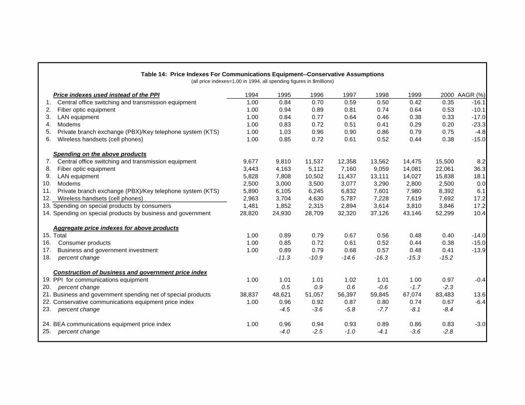
Price indexes used instead of the PPI 1994 1995 1996 1997 1998 1999 2000 AAGR (%)1. Central office switching and transmission equipment 1.00 0.84 0.70 0.59 0.50 0.42 0.35 -16.12. Fiber optic equipment 1.00 0.94 0.89 0.81 0.74 0.64 0.53 -10.13. LAN equipment 1.00 0.84 0.77 0.64 0.46 0.38 0.33 -17.04. Modems 1.00 0.83 0.72 0.51 0.41 0.29 0.20 -23.35. Private branch exchange (PBX)/Key telephone system (KTS) 1.00 1.03 0.96 0.90 0.86 0.79 0.75 -4.86. Wireless handsets (cell phones) 1.00 0.85 0.72 0.61 0.52 0.44 0.38 -15.0

Spending on the above products

7. Central office switching and transmission equipment 9,677 9,810 11,537 12,358 13,562 14,475 15,500 8.28. Fiber optic equipment 3,443 4,163 5,112 7,160 9,059 14,081 22,061 36.39. LAN equipment 5,828 7,808 10,502 11,437 13,111 14,027 15,838 18.1

10. Modems 2,500 3,000 3,500 3,077 3,290 2,800 2,500 0.011. Private branch exchange (PBX)/Key telephone system (KTS) 5,890 6,105 6,245 6,832 7,601 7,980 8,392 6.112. Wireless handsets (cell phones) 2,963 3,704 4,630 5,787 7,228 7,619 7,692 17.213. Spending on special products by consumers 1,481 1,852 2,315 2,894 3,614 3,810 3,846 17.214. Spending on special products by business and government 28,820 24,930 28,709 32,320 37,126 43,146 52,299 10.4

Aggregate price indexes for above products15. Total 1.00 0.89 0.79 0.67 0.56 0.48 0.40 -14.016. Consumer products 1.00 0.85 0.72 0.61 0.52 0.44 0.38 -15.017. Business and government investment 1.00 0.89 0.79 0.68 0.57 0.48 0.41 -13.918. percent change -11.3 -10.9 -14.6 -16.3 -15.3 -15.2

Construction of business and government price index

19. PPI for communications equipment 1.00 1.01 1.01 1.02 1.01 1.00 0.97 -0.420. percent change 0.5 0.9 0.6 -0.6 -1.7 -2.321. Business and government spending net of special products 38,837 48,621 51,057 56,397 59,845 67,074 83,483 13.622. Conservative communications equipment price index 1.00 0.96 0.92 0.87 0.80 0.74 0.67 -6.423. percent change -4.5 -3.6 -5.8 -7.7 -8.1 -8.4

24. BEA communications equipment price index 1.00 0.96 0.94 0.93 0.89 0.86 0.83 -3.025. percent change -4.0 -2.5 -1.0 -4.1 -3.6 -2.8

Table 14: Price Indexes For Communications Equipment--Conservative Assumptions

(all price indexes=1.00 in 1994, all spending figures in $millions)

Price indexes used instead of the PPI 1994 1995 1996 1997 1998 1999 2000 AAGR (%)

1.Items from conversative assumptions page with adjustment for PBX prices falling an additional 1 percent per year 1.00 0.88 0.79 0.67 0.56 0.47 0.40 -14.2

2. Other data commnication 1.00 0.88 0.83 0.72 0.57 0.49 0.44 -12.73. Voice processing equipment (call centers, voice mail,..) 1.00 1.03 0.96 0.90 0.86 0.79 0.75 -4.84. Cellular phone infrastructure 1.00 0.93 0.86 0.79 0.73 0.68 0.63 -7.55. Cable TV equipment 1.00 0.95 0.90 0.86 0.81 0.77 0.74 -5.0

Spending on special products6. Items from conversative assumptions page 28,820 24,930 28,709 32,320 37,126 43,146 52,299 10.47. Other data commnication 4,902 6,567 8,834 9,620 11,344 13,479 15,532 21.28. Voice processing equipment (call centers, voice mail,..) 4,279 4,435 4,537 4,963 5,626 6,215 6,743 7.99. Cellular phone infrastructure 4,266 4,693 5,162 5,678 4,474 4,955 4,734 1.8

10. Cable TV equipment 2,554 2,810 3,091 3,400 3,850 5,400 6,000 15.311. Spending on special products by business and government 44,821 43,435 50,332 55,981 62,420 73,195 85,308 11.3

Aggregate price indexes for special products

12. Business and government investment 1.00 0.91 0.83 0.73 0.62 0.54 0.48 -11.613. percent change -9.4 -8.8 -12.0 -14.5 -12.9 -12.1

Construction of business and government price index Assume PPI falls 2 percent per year faster than actual

14. Modified PPI for communications equipment 1.00 0.99 0.97 0.96 0.94 0.90 0.86 -2.4

15. Moderate communications equipment price index 1.00 0.94 0.88 0.81 0.73 0.66 0.60 -8.316. percent change -6.4 -5.8 -8.1 -10.2 -9.7 -9.3

17. BEA communications equipment price index 1.00 0.96 0.94 0.93 0.89 0.86 0.83 -3.018. percent change -4.0 -2.5 -1.0 -4.1 -3.6 -2.8

19. BEA computer price index 1.00 0.84 0.64 0.49 0.36 0.28 0.24 -21.220. percent change -16.1 -24.0 -22.5 -26.4 -23.8 -13.6

Table 15: Price Indexes For Communications Equipment--Moderate Assumptions

(all price indexes=1.00 in 1994, all spending figures in $millions)

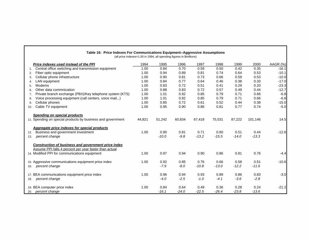
Price indexes used instead of the PPI 1994 1995 1996 1997 1998 1999 2000 AAGR (%)1. Central office switching and transmission equipment 1.00 0.84 0.70 0.59 0.50 0.42 0.35 -16.12. Fiber optic equipment 1.00 0.94 0.89 0.81 0.74 0.64 0.53 -10.13. Cellular phone infrastructure 1.00 0.90 0.81 0.73 0.66 0.59 0.53 -10.04. LAN equipment 1.00 0.84 0.77 0.64 0.46 0.38 0.33 -17.05. Modems 1.00 0.83 0.72 0.51 0.41 0.29 0.20 -23.36. Other data commnication 1.00 0.88 0.83 0.72 0.57 0.49 0.44 -12.77. Private branch exchange (PBX)/Key telephone system (KTS) 1.00 1.01 0.92 0.85 0.79 0.71 0.66 -6.88. Voice processing equipment (call centers, voice mail,..) 1.00 1.01 0.92 0.85 0.79 0.71 0.66 -6.89. Cellular phones 1.00 0.85 0.72 0.61 0.52 0.44 0.38 -15.0

10. Cable TV equipment 1.00 0.95 0.90 0.86 0.81 0.77 0.74 -5.0

Spending on special products11. Spending on special products by business and government 44,821 51,242 60,834 67,418 75,531 87,222 101,146 14.5

Aggregate price indexes for special products12. Business and government investment 1.00 0.90 0.81 0.71 0.60 0.51 0.44 -12.613. percent change -10.0 -9.8 -13.2 -15.5 -14.0 -13.3

Construction of business and government price indexAssume PPI falls 4 percent per year faster than actual

14. Modified PPI for communications equipment 1.00 0.97 0.94 0.90 0.86 0.81 0.76 -4.4

15. Aggressive communications equipment price index 1.00 0.92 0.85 0.76 0.66 0.58 0.51 -10.616. percent change -7.9 -8.0 -10.8 -13.0 -12.2 -11.6

17. BEA communications equipment price index 1.00 0.96 0.94 0.93 0.89 0.86 0.83 -3.018. percent change -4.0 -2.5 -1.0 -4.1 -3.6 -2.8

19. BEA computer price index 1.00 0.84 0.64 0.49 0.36 0.28 0.24 -21.220. percent change -16.1 -24.0 -22.5 -26.4 -23.8 -13.6

Table 16: Price Indexes For Communications Equipment--Aggressive Assumptions

(all price indexes=1.00 in 1994, all spending figures in $millions)

1994 1995 1996 1997 1998 1999 2000 AAGR (%)Conservative 1.00 0.96 0.92 0.87 0.80 0.74 0.67 -6.4 percent change -4.5 -3.6 -5.8 -7.7 -8.1 -8.4

Moderate 1.00 0.94 0.88 0.81 0.73 0.66 0.60 -8.3 percent change -6.4 -5.8 -8.1 -10.2 -9.7 -9.3

Aggressive 1.00 0.92 0.85 0.76 0.66 0.58 0.51 -10.6 percent change -7.9 -8.0 -10.8 -13.0 -12.2 -11.6

BEA communications equipment 1.00 0.96 0.94 0.93 0.89 0.86 0.83 -3.0 percent change -4.0 -2.5 -1.0 -4.1 -3.6 -2.8

BEA computers 1.00 0.84 0.64 0.49 0.36 0.28 0.24 -21.20 percent change -16.1 -24.0 -22.5 -26.4 -23.8 -13.6

Table 17: Summary of price indexes for communications equipment(all price indexes=1.00 in 1994)

Increase in average annual growth from 1994 to 2000

Communications equipment

Information processing equipment

Non-residential investment

Conservative 4.1 0.9 0.4

Moderate 6.6 1.5 0.6

Aggressive 9.8 2.2 0.9

Table 18: Changes in Average Annual Growth Rates for Real Investment Using Various Price Indexes for Communications Equipment