Comparative Study on Different CFD Solvers for Analysis of

11th International Workshop on Ship and Marine Hydrodynamics Hamburg, Germany, September 22-25, 2019

Comparative Study on Different CFD Solvers for Analysis of Ship Added

Resistance

Byung-Soo Kim1, Kyung-Kyu Yang2, Zhang Zhu1, Yonghwan Kim1,*

1Seoul National University, Department of Naval Architecture and Ocean Engineering 1, Gwanak-ro, Gwanak-gu, Seoul, Republic of Korea

2Korea Research Institute of Ships & Ocean Engineering 32, Yuseong-daero 1312beon-gil, Yuseong-gu, Daejeon, Republic of Korea

*Corresponding author, [email protected]

ABSTRACT

This study deals with motion responses and the added resistance of the ship in waves using computational fluid dynamics (CFD). In this study, motion response and the added resistance of the modified blunt Wigley are investigated using two types of CFD program: SNU-MHL-CFD (Seoul National University Marine Hydrodynamics Laboratory CFD) and OpenFOAM. SNU-MHL-CFD is Euler equation solver which is an in-house code based on a Cartesian-grid and immersed boundary method. OpenFOAM is Reynolds-Averaged Navier-Stokes (RANS) equation solvers which is an open source library. Before solving the ship motion in waves, hydrodynamic coefficients are calculated by forced heave and pitch motions and wave excitation forces/moments are computed from wave diffraction problem without any hull motion. Three types of solvers are used: two previously mentioned solvers and additionally commercial software, Star-CCM+. These results are validated with the experimental data. Finally, ship motion responses and added resistance in waves are compared with available experimental data and their computational costs are compared.

1 INTRODUCTION

Ship added resistance in waves is a widely studied seakeeping problem that has been carried out from the past. Traditionally, potential flow based methods have been used to investigate the ship performance in waves. A study done by Kim and Kim [1], which analyzed ship added resistance by using the Rankine panel method, is a typical example. However, potential theories are mostly based on the linear assumption without viscosity terms. Consequently, many recent studies are using CFD methods to further investigate the added resistance by considering the nonlinear effects and viscous flow patterns around the ships. Many different types of solvers are developed throughout the past several decades. In the beginning, many groups had started to develop their own in-house codes to simulate the flow and still many groups are developing their own CFD codes. Yang et al. [2] developed an in-house CFD code using the Cartesian-based method and simulated the motion and ship added resistance for WigleyIII hull and S175 containership. Also, Yang and Kim [3] used developed CFD code to investigate the influence of bow shapes of KRISO’s very large crude oil carrier (KVLCC) to the added resistance in short wavelengths. As personal computers develop rapidly with high performances, many companies started to develop commercial software like Fluent and Star-CCM+ and they are widely used nowadays due to a user-friendly interface. Simonsen et al. [4] compared the ship response of KRISO Container Ship (KCS) using CFDSHIP-IOWA and Star-CCM+. Tezdogan et al. [5] compared motion and the added resistance of full-scale KCS using commercial software Star-CCM+ and also showed the effect of slow steaming. Most recently, open source CFD library like OpenFOAM is widely used and many codes are being developed based on these kinds of open source libraries. Ye et al. [6] used

2

naoe-FOAM-SJTU, which is a modified version based on original OpenFOAM, to compute the added resistance and ship motion of S-175 containership.

In this study, motion responses and added resistance of modified blunt Wigley is studied using a different type of CFD solvers: in-house code, SNU-MHL-CFD, open source CFD code, OpenFOAM and commercial software, Star-CCM+. These different kinds of solvers have their own combination of methods to solve the problem and details about these solvers will be mentioned later. Before calculating the motion responses and added resistance, hydrodynamic coefficients and wave excitation forces and moments are confirmed by solving radiation problems and diffraction problems. Similar conditions are used for each solver to compare the solvers.

2 NUMERICAL METHODS

2.1 SNU-MHL-CFD

SNU-MHL-CFD is an in-house code developed by Yang et al. [2] and only brief explanations will be stated here. In this code, the Cartesian grid with a finite volume method was used. Instead of solving Navier-Stokes equations, viscous terms are neglected and Euler equations (equation (1), Yang et al. [2]) are solved with the continuity equation. This means that only nonlinear effects are included. Each cell is divided into three phases (solid, liquid, and gas) and volume fraction is used to indicate the free surface and the body shape. The interface capturing method was used to capture the free surface behavior. The ship is represented by the level-set method using the signed distance function. Ship motions are solved using the immersed boundary method. Finally, the fractional step method was used to solve the pressure-velocity coupling problem.

( ) 1dV dS p dS dVt ρΩ Γ Γ Ω

∂+ ⋅ = − + ∂

∫ ∫ ∫ ∫ bu u u n n f (1)

2.2 OpenFOAM

OpenFOAM is an open source C++ CFD library for solving different kinds of problems. Since every step of the simulation can be modified by the user and there are no additional costs to pay, it is widely used recently. In order to generate the mesh, blockMesh utility, and snappyHexMesh utility, which are basic utilities provided in OpenFOAM were used. OpenFOAM contains many different solvers and in this study, waves2Foam solver [7] was used to simulate the waves and flow patterns near the hull. Flows are solved by solving incompressible RANS equations (equation (2), Jacobsen et al. [7]) with the continuity equation as a constraint. SST k-ω model was used to model the Reynolds stress term. For the interface, the Volume Of Fluid (VOF) method was used and the forcing method was adapted to generate and damp the waves better. When the ship moves, meshes near the ship are deformed together. This means that between several methods that can be used to simulate ship motion like overset mesh technique and mesh deformation technique, the mesh deformation technique is used. To solve the pressure field, the Pressure-Implicit Split-Operator (PISO) algorithm was used.

[ ]*TTp

t γρ ρ ρ µ ρ σ κ γ∂ +∇ ⋅ = −∇ − ⋅ ∇ +∇ ⋅ ∇ + + ∇ ∂

u uu g x u τ (2)

2.3 Star-CCM+

Star-CCM+ is a commercial CFD software widely used from companies to universities. Star-CCM+ is RANS based solver using a finite volume method, which is similar to OpenFOAM and many other CFD solvers. In this study, the realizable k-ε model was selected for the Reynolds stress term and the interface was captured by using the VOF method. Mesh deformation technique is adopted to simulate the ship motion for the forced heave motion and the pressure is obtained from the Semi-Implicit Method for Pressure-Linked Equations (SIMPLE) method.

3

3 CALCULATION CONDITIONS

3.1 Calculation Model

The modified blunt Wigley model is selected as a test hull for this study. Modified blunt Wigley is mathematically defined hull using equation (3) and the hull shape is rather simple compared to the typically designed hull. There are several experiments done by Kashiwagi [8] and He and Kashiwagi [9]. The mathematical expression of this hull is like below, where x’ = x/(L/2), y’ = y/(B/2), and z’ = z/T. Here, L is ship length, B is ship breadth and T is ship draught. The model ship is illustrated in Figure 1 and the model scale used for this study is summarized in Table 1.

( )( )( ) ( )( )42 2 2 4 2 8 21 1 1 0.6 1 1y z x x x z z x′ ′ ′ ′ ′ ′ ′ ′= − − + + + − − (3)

Figure 1: Hull of modified blunt Wigley

Table 1: Main properties of modified blunt Wigley

Properties Values Ship length (L) 2.500 [m]

Ship breadth (B) 0.500 [m] Ship draught (T) 0.175 [m]

Displacement, (∇) 0.1388 [m3] Froude number (Fn) 0.200

3.2 Calculation conditions

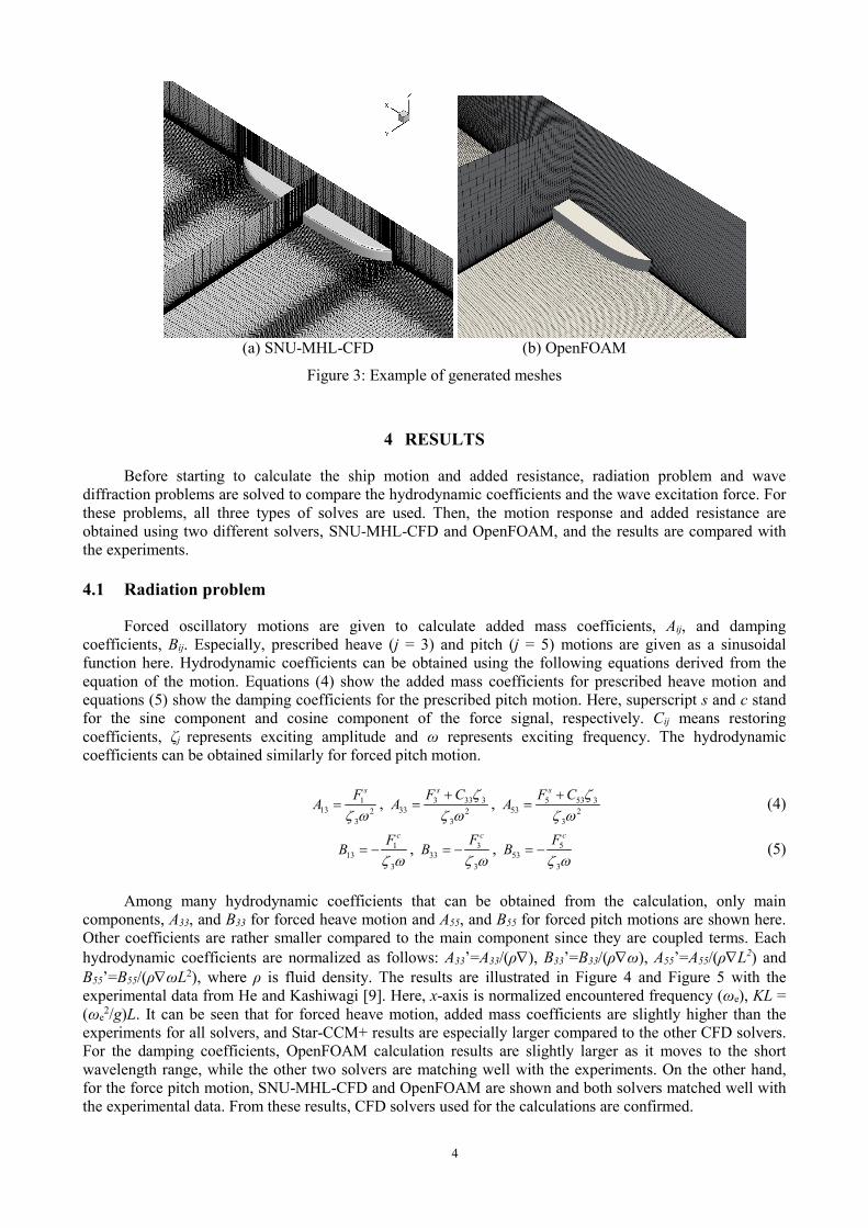
Calculation conditions are selected to be similar for both code, but some differences are inevitable since they solve different governing equations using a different type of meshes and a different type of physical modeling. In other words, because the convergence rate is different for each code, some properties are not exactly the same. For SNU-MHL-CFD, as mentioned earlier, the Cartesian grid was generated with more than 75 meshes per wavelength and more than 15 meshes per wave height. For OpenFOAM, nearly 150 meshes per wavelength and 15 meshes per wave height were generated by the blockMesh utility and then the hull is carved out by snappyHexMesh utility with the addition of layers near the hull. Figure 2 and Figure 3 show the domain size used for the calculations and the example of the generated meshes.

(a) SNU-MHL-CFD (b) OpenFOAM

Figure 2: Domain size used for the calculation

4

(a) SNU-MHL-CFD (b) OpenFOAM

Figure 3: Example of generated meshes

4 RESULTS

Before starting to calculate the ship motion and added resistance, radiation problem and wave diffraction problems are solved to compare the hydrodynamic coefficients and the wave excitation force. For these problems, all three types of solves are used. Then, the motion response and added resistance are obtained using two different solvers, SNU-MHL-CFD and OpenFOAM, and the results are compared with the experiments.

4.1 Radiation problem

Forced oscillatory motions are given to calculate added mass coefficients, Aij, and damping coefficients, Bij. Especially, prescribed heave (j = 3) and pitch (j = 5) motions are given as a sinusoidal function here. Hydrodynamic coefficients can be obtained using the following equations derived from the equation of the motion. Equations (4) show the added mass coefficients for prescribed heave motion and equations (5) show the damping coefficients for the prescribed pitch motion. Here, superscript s and c stand for the sine component and cosine component of the force signal, respectively. Cij means restoring coefficients, ζj represents exciting amplitude and ω represents exciting frequency. The hydrodynamic coefficients can be obtained similarly for forced pitch motion.

1

13 23

sFAζ ω

= , 3 33 333 2

3

sF CA

ζζ ω+

= , 5 53 353 2

3

sF CA

ζζ ω+

= (4)

113

3

cFBζ ω

= − , 333

3

cFB

ζ ω= − , 5

533

cFB

ζ ω= − (5)

Among many hydrodynamic coefficients that can be obtained from the calculation, only main

components, A33, and B33 for forced heave motion and A55, and B55 for forced pitch motions are shown here. Other coefficients are rather smaller compared to the main component since they are coupled terms. Each hydrodynamic coefficients are normalized as follows: A33’=A33/(ρ∇), B33’=B33/(ρ∇ω), A55’=A55/(ρ∇L2) and B55’=B55/(ρ∇ωL2), where ρ is fluid density. The results are illustrated in Figure 4 and Figure 5 with the experimental data from He and Kashiwagi [9]. Here, x-axis is normalized encountered frequency (ωe), KL = (ωe

2/g)L. It can be seen that for forced heave motion, added mass coefficients are slightly higher than the experiments for all solvers, and Star-CCM+ results are especially larger compared to the other CFD solvers. For the damping coefficients, OpenFOAM calculation results are slightly larger as it moves to the short wavelength range, while the other two solvers are matching well with the experiments. On the other hand, for the force pitch motion, SNU-MHL-CFD and OpenFOAM are shown and both solvers matched well with the experimental data. From these results, CFD solvers used for the calculations are confirmed.

5

KL

A33

/(ρ∇

)

0 5 10 15 20 25 300

0.2

0.4

0.6

0.8

1

1.2

1.4

1.6

1.8

2 A 33, Exp. (He & Kashiwagi, 2014)A 33, Star-CCM+A 33, OpenFOAMA 33, SNU-MHL-CFD

KL

B33

/(ρω∇

)

0 5 10 15 20 25 300

0.2

0.4

0.6

0.8

1

1.2

1.4

1.6

1.8

2B33, Exp. (He & Kashiwagi, 2014)B33, Star-CCM+B33, OpenFOAMB33, SNU-MHL-CFD

(a) A33’ (added mass) (b) B33’ (damping)

Figure 4: Hydrodynamic coefficients of modified blunt Wigley for forced heave oscillation

KL

A55

/(ρ∇

L2 )

0 5 10 15 20 25 30-0.2

-0.1

0

0.1

0.2 A 55, Exp. (He & Kashiwagi, 2014)A 55, OpenFOAMA 55, SNU-MHL-CFD

KL

B55

/(ρω∇

L2 )

0 5 10 15 20 25 30-0.2

-0.1

0

0.1

0.2 B 55, Exp. (He & Kashiwagi, 2014)B 55, OpenFOAMB 55, SNU-MHL-CFD

(a) A55’ (added mass) (b) B55’ (damping)

Figure 5: Hydrodynamic coefficients of modified blunt Wigley for forced pitch oscillation

4.2 Diffraction problem

In order to calculate wave exciting force, the ship is fixed without any motion and the wave hits the ship. Then the force and moments due to waves are calculated. Wave amplitudes are selected to be fixed at 0.03m and when the wavelength is short, wave steepness is chosen to be less than 1/30. These conditions are analogous to the wave conditions used in Kashiwagi [8]. Having the same wave conditions are important because CFD solvers account nonlinear effect. From the obtained force signals, wave excitation amplitudes are calculated using Fourier analysis and are normalized with a combination of density, gravity, wave amplitude, ship breadth, and ship length. The results are plotted in Figure 6 with experiments conducted by Kashiwagi [8]. As can be seen from the plotted pictures, three codes show similar behavior. All the calculations show slightly less surge exciting forces compared to the experiments, but they show similar values with each other. For the heave exciting forces and pitch exciting moments, computation results are similar to the experiments. From these results, it can be confirmed that all three solvers properly generate the waves and illustrate the body shape well.

6

λ / L

|E1|

/(ρg

AB

L)

0 0.5 1 1.5 20

0.1

0.2

0.3

0.4

0.5|E1|, Exp. (Kashiwagi, 2013)|E1|, Star-CCM+|E1|, OpenFOAM|E1|, SNU-MHL-CFD

Amax/L=0.012

λ / L

|E3|

/(ρg

AB

L)

0 0.5 1 1.5 20

0.1

0.2

0.3

0.4


Amax/L=0.012

(a) Surge exciting force (b) Heave exciting force

λ / L

|E5|

/(ρg

AB

L2 )

0 0.5 1 1.5 20

0.05

0.1

0.15


Amax/L=0.012

(c) Pitch exciting moment

Figure 6: Wave exciting forces and moments of modified blunt Wigley in a head sea

4.3 Motion and added resistance

In order to solve the motion response and the added resistance of the ship, 2 degrees of motions, heave, and pitch, are freed in head waves. Wave conditions are the same as the conditions used for the diffraction problem. Simulations are done for 15 encountering periods to obtain converged data. From the converged motion signals, Fourier analysis was used to obtain the motion amplitude and then it is normalized to obtain the response amplitude operator. For the added resistance, the mean value from the unsteady calculations is obtained and the steady resistance is subtracted from it. Steady calculations are additionally done for each case to obtain steady resistance since the meshes are different for every wavelength.

The wavelengths are modified from half the ship length to twice the ship length. Obtained motion and force signals for three cases, one from short wavelength, near resonance wavelength, and long wavelength, are shown in Figure 7. Here as mentioned earlier, only two solvers, SNU-MHL-CFD and OpenFOAM, are compared. The above pictures are signals from SNU-MHL-CFD and the below pictures are signals from OpenFOAM. As viscous terms are included in OpenFOAM solver, the force from pressure and force from the viscosity are plotted separately. It can be confirmed that both solvers show similar pressure force signal patterns with similar phases. Especially, near the resonance frequency, although there is high nonlinearity in force signals, both patterns are alike. Also, viscous force components are rather smaller compared to the pressure forces. Motion signals are also similar although there is a slight difference in amplitude.

7

(a) Time signal for short wavelength (λ/L = 0.5)

(b) Time signal near resonance wavelength (λ/L = 1.1)

(c) Time signal for long wavelength (λ/L = 2.0)

Figure 7: Motion and force time signals of modified blunt Wigley in a head sea for different wavelengths

Next wave contours for two solvers are shown for the same wavelength conditions. Both x-direction

and y-direction are normalized with the ship length and the wave elevation is normalized with wave amplitude. As can be seen from Figure 8, the absolute value of normalized wave elevation is selected to be less than 1.2 of the wave amplitude. For the short wavelength, the flow patterns are most different compare to the other cases. Although the flow pattern near the hull is similar, flows that are far from the hull are rather different. An OpenFOAM calculation shows a more damped wave elevation compare to the wave elevation

8

from SNU-MHL-CFD. There might be several reasons for this including different mesh and different governing equations, the main reason for this might be due to reflected waves. Although it is not significant for the other wavelengths, as wave height is smaller for short wavelength, reflected waves might have played an important role in reducing the wave height. Further studies should be done to reduce this reflection. For the frequency near the resonance and the long wave, wave contours show similar wave patterns along the hull and similar stern flows, respectively.

(a) Wave contours for short wavelength (λ/L = 0.5, left: SNU-MHL-CFD, right: OpenFOAM)

(b) Wave contours near resonance wavelength (λ/L = 1.1, left: SNU-MHL-CFD, right: OpenFOAM)

(c) Wave contours for long wavelength (λ/L = 2.0, left: SNU-MHL-CFD, right: OpenFOAM)

Figure 8: Wave contours of modified blunt Wigley in a head sea for different wavelengths

Calculated results over a wide range of wavelengths are shown in Figure 9 and Figure 10 with the

experimental data from Kashiwagi [8] and the experiments from Seoul National University (SNU). Note that the experiments from SNU are conducted with a fixed wave height of H/L = 0.013. However, there is no significant discrepancy between two experiments and the only slight difference can be found in heave motion. Figure 9 shows the results of the motion response with respect to the wavelength and it can be seen that both solvers show a similar tendency with both experiments. However, OpenFOAM results show some differences when the wavelength is near 1.6 of the ship length. Figure 10 shows the added resistance of modified blunt Wigley. Similarly, although the overall tendency is similar for both solvers, SNU-MHL-CFD has a tendency to underestimate the added resistance at the short wavelength, while OpenFOAM results overestimate the added resistance at 1.3 of the ship length. It can be seen that viscous effects are not that significant in overall results for added resistance. However, for simulations including highly separated flow patterns and when the other motions are included, especially roll motion, viscous effect will play important role and this term must be accounted.

9

λ / L

ξ 3/A

0 0.5 1 1.5 2 2.500.20.40.60.8

11.21.41.61.8

2Exp. (SNU), H/L=0.013Exp. (Kashiwagi, 2013), Amax/L=0.012OpenFOAM, Amax/L=0.012SNU-MHL-CFD, Amax/L=0.012

λ / L

ξ 5/k

A

0 0.5 1 1.5 2 2.500.20.40.60.8

11.21.41.61.8


(a) Heave motion response (b) Pitch motion response

Figure 9: Motion response of modified blunt Wigley in a head sea

λ / L

R/(ρg

A2 B

2 /L)

0 0.5 1 1.5 2 2.50

4

8

12


Figure 10: Added resistance of modified blunt Wigley in a head sea

Table 2: Numerical parameters and computation costs for different CFD solvers

Properties SNU-MHL-CFD OpenFOAM Mesh Number 3M – 5M 4M – 7M

Te/Δt 250 (adjustable) 500 # of cores 1 16 Ttotal/(Te#) 4.8 – 7.2 hours 4 – 11 hours

Finally, computation costs for both solvers are compared since CFD still takes a lot of time to compute

which means that more efficient calculations are still needed. Related details are summarized in Table 2. About similar grid numbers are used since mesh number plays an important role in calculation time. Time steps are slightly different, but for both cases, it is set to have a CFL number nearly unity. Parallel computing is not yet built in SNU-MHL-CFD while OpenFOAM has parallel computing functions. However, although the parallel computing was used in OpenFOAM with 16 cores, total simulation time is not much different from the SNU-MHL-CFD and this might be related to the computation of turbulence modeling. Also, communication time between cores might be another reason for this. As a result, it can be interpreted that SNU-MHL-CFD might be a more efficient solver for calculating ship motions and added resistance since more computation can be done on leftover cores.

10

5 CONCLUSIONS

In this study, two types of CFD solvers are used to calculate hydrodynamic coefficients for heave and pitch motions and wave excitation forces and moments. They are confirmed for modified blunt Wigley with forward speed. Moreover, the motion response and added resistance were also calculated using two different types of CFD solvers. The following results are made here. - Euler equation solver, SNU-MHL-CFD, and RANS solver, OpenFOAM, both showed comparable results with the experimental data. Hydrodynamic coefficients for both heave and pitch motions matched well with the experiments and the wave excitation forces and moments also fitted well with the experimental trend. - Time signals and wave contours for the short wavelength, wavelength near resonance, and long wavelength are compared for both solvers. Time signal patterns matched well with each other. Wave contours for each solver are plotted for different wavelengths. Wave contours showed a slight difference in flow patterns for short wavelengths, however, flow patterns near the hull body were similar. For the resonance wavelength and the long wavelength, flow patterns were alike. - Obtained motion responses and the added resistance for two solvers are compared with the experiments and showed a similar tendency. It can be seen that the viscosity effect is not as important for the calculation of motion responses and added resistance in head wave conditions unless there is highly severe separation. - Computation costs for both solvers are compared. Although SNU-MHL-CFD does not have parallel computing functions, the ignorance of the viscosity term might have resulted in faster computation time compare to the OpenFOAM.

ACKNOWLEDGEMENTS

This study was supported by the Ministry of Trade, Industry and Energy (MOTIE), Korea, through the project number 10062881, “Technology Development to Improve Added Resistance and Ship Operational Efficiency for Hull Form Design”. Their supports are appreciated. Moreover, supports from the Lloyd’s Register Foundation (LRF)-Funded Research Center at Seoul National University are also respected.

REFERENCES

[1] Kim, K.H., and Kim, Y. “Numerical study on added resistance of ships by using a time-domain Rankine panel method” In: Ocean Engineering, 38(13) (2011), 1357-1367

[2] Yang, K.K., Kim, Y. and Nam, B.W. “Cartesian-grid-based computational analysis for added resistance in waves”. In: Journal of Marine Science and Technology, 20 (2015), 155-170

[3] Yang, K.K. and Kim, Y. “Numerical analysis of added resistance on blunt ships with different bow shapes in short waves”. In: Journal of Marine Science and Technology, 22 (2017), 245-258

[4] Tezdogan, T., Demirel, Y.G., Kellett, P., Khorasanchi, M., Incecik, A., and Turan, O. “Full-scale unsteady RANS CFD simulations of ship behaviour and performance in head seas due to slow steaming”. In: Ocean Engineering, 97 (2015), 186-206

[5] Simonsen, C.D., Otzen, J.F., Joncquez, S. and Stern, F. “EFD and CFD for KCS heaving and pitching in regular head waves”. In: Journal of Marine Science and Technology, 18 (2013), 435-459

[6] Ye, H., Shen, Z., and Wan, D. “Numerical prediction of added resistance and vertical ship motions in regular head waves.” In: Journal of Marine Science and Application, 11(2012), 410-416

[7] Jacobsen, N.G., Fuhrman, D.R., and Fredsøe, J. “A wave generation toolbox for the open-source CFD library: OpenFOAM®”. In: International Journal of Numerical Methods in Fluids, 70 (2012), 1073-1088

[8] Kashiwagi, M., “Hydrodynamic Study on Added Resistance Using Unsteady Wave Analysis”. In: Journal of Ship Research, 57(4) (2013), 220-240.

[9] He, G. and Kashiwagi, M. “A time-domain higher-order boundary element method for 3D forward-speed radiation and diffraction problems”. In: Journal of Marine Science and Technology, 19 (2014), 228-244

Documents

Comparative Study on Different CFD Solvers for Analysis of