Comparison of HVAC system modeling in EnergyPlus, DeST and ... · In the integrated test cases part, based on the review of existing HVAC system tests, an integrated test method is

Research Article

Building Systems and

Components

E-mail: [email protected]

Comparison of HVAC system modeling in EnergyPlus, DeST and DOE-2.1E

Xin Zhou1, Tianzhen Hong2, Da Yan1 ()

1 Department of Building Science, School of Architecture, Tsinghua University, Beijing 100084, China 2 Lawrence Berkeley National Laboratory, 1 Cyclotron Road, Berkeley, CA 94720, USA Abstract Building energy modeling programs (BEMPs) are effective tools for evaluating the energy savings potential of building technologies and optimizing building design. However, large discrepancies in simulated results from different BEMPs have raised wide concern. Therefore, it is strongly needed to identify, understand, and quantify the main elements that contribute towards the discrepancies in simulation results. ASHRAE Standard 140 provides methods and test cases for building thermal load simulations. This article describes a new process with various methods to look inside and outside the HVAC models of three BEMPs—EnergyPlus, DeST, and DOE-2.1E—and compare them in depth to ascertain their similarities and differences. The article summarizes methodologies, processes, and the main modeling assumptions of the three BEMPs in HVAC calculations. Test cases of energy models are designed to capture and analyze the calculation process in detail. The main findings are: (1) the three BEMPs are capable of simulating conventional HVAC systems, (2) matching user inputs is key to reducing discrepancies in simulation results, (3) different HVAC models can be used and sometimes there is no way to directly map between them, and (4) different HVAC control strategies are often used in different BEMPs, which is a driving factor of some major discrepancies in simulation results from various BEMPs. The findings of this article shed some light on how to compare HVAC calculations and how to control key factors in order to obtain consistent results from various BEMPs. This directly serves building energy modelers and policy makers in selecting BEMPs for building design, retrofit, code development, code compliance, and performance ratings.

Keywords building energy modeling programs,

comparative tests,

DeST,

DOE-2.1E,

EnergyPlus,

HVAC,

system modeling Article History Received: 22 March 2013

Revised: 11 July 2013

Accepted: 12 July 2013 © Tsinghua University Press and

Springer-Verlag Berlin Heidelberg

2013

1 Introduction

Computer simulation is one of the most effective and economical methods to predict and analyze building energy consumption and performance. The simulation industry has developed rapidly since the 1960s, with hundreds of building energy modeling programs (BEMPs) developed and used around the world. Well known BEMPs include DOE-2 and EnergyPlus from the U.S. Department of Energy, ESP-r from the University of Strathclyde, U.K., and DeST from Tsinghua University, China. These BEMPs are widely used in the design stages of new energy efficient buildings, the planning stages of energy retrofits for existing buildings, and the development of building energy codes and standards and energy labeling programs in the building

industry. However, an increasing number of practical applications have shown that large discrepancies exist in results from different modelers using different BEMPs for the same building. This is a large problem for the simulation industry and is consequently the subject of more attention. Some believe that the simulation methodology is flawed and attribute the discrepancies to the different calculation engines of different BEMPs. This lack in confidence may hinder the development and application of BEMPs. Consequently, it is important for the simulation industry to understand the reasons for these discrepancies and define the application scope of each program. To solve the problem and promote the development of BEMPs, detailed comparison of BEMPs’ calculation engines is a fundamental and significant step.

BUILD SIMUL (2014) 7: 21–33 DOI 10.1007/s12273-013-0150-7

Zhou et al. / Building Simulation / Vol. 7, No. 1

22

Simulating the energy use of buildings is a complex process. It is difficult to ascertain the weakness or faults of simulation programs. Continuous and systematic validation work is needed for simulation programs. The validation work of BEMPs includes a combination of empirical validation, analytical verification, and comparative analysis techniques (Judkoff and Neymark 2006). For comparison purposes, BEMPs can be divided into two parts: the load-side cal-culations and the HVAC system-side calculations, as Fig. 1 shows. Several organizations that specialize in building energy simulation have released standards and guidelines for the validation process, including IEA (International Energy Agency) BESTest (Judkoff and Neymark 1995) and ASHRAE Standard 140 (ANSI/ASHRAE 2007). A number of studies have been conducted to compare the advantages and disadvantages of several BEMPs (Crawley et al. 2008).

The testing and validation work is well developed and widely recognized for the building loads calculations. Many simulation programs have gone through comparative loads tests. Existing loads tests cover the building envelope, window shading, interior solar distribution, and thermal mass—all factors that drive loads simulations. Most popular simulation programs such as EnergyPlus, DeST, DOE-2, ESP, BLAST, and TRNSYS have participated in several of these tests.

Another important component of building energy simulation is the HVAC system calculation. The HVAC tests based on ASHRAE research project 865 (Yuill and Haberl 2002) offer several analytical tests. The ANSI/ASHRAE Standard 140 offers several test cases for simple unitary vapor compression cooling systems and fuel-fired furnace heating systems (ANSI/ASHRAE 2007; Neymark and Judkoff 2002; Purdy and Beausoleil-Morrison 2003). One of the tests created under IEA SHC Task 34/ECBCS Annex 43 examines the mechanical equipment and control strategies for chilled water and hot water systems. This tests the performance and control strategies of chillers, cooling/heating coils, chilled water hydraulic circuits, boilers, and hot water hydraulic circuits (Felsmann 2008; Henninger and Witte 2011a). Developers of some simulation programs have

created several test cases to verify their simulation results. For example, the EnergyPlus global energy balance tests check the accuracy of EnergyPlus with regards to energy balances at various boundary volumes when simulating the operation of HVAC systems (Henninger and Witte 2011b). There are a few HVAC tests done for EnergyPlus (Henninger and Witte 2011c, d, e, f).

However, the tests for HVAC systems still need a standardized and easily adopted method to allow their implementation in a structured and consistent way. The inter-program comparison of HVAC system calculations for commonly used BEMPs is of great significance for users to gain a better understanding of each simulation program. This will also lead to a more effective use of building simulation in scientific research and engineering practice.

Based on these understandings, this article summarizes methodologies, processes, and the main assumptions of three widely-used BEMPs: EnergyPlus, DeST, and DOE-2.1E. The comparison work regarding load-side calculations has been published in another article (Zhu et al. 2013). This article focused on the solution algorithms of the HVAC systems, component models, how control strategies are modeled, and what default inputs are used in the three BEMPs.

The objectives of the comparison include: (1) Based on the technical documentation and source code

of the three BEMPs, summarize their main advantages and disadvantages, including calculation procedures, component models, and control strategies, to gain a better understanding of the HVAC system calculations in each program, including the simulation structure, application scope, and modeling limitations.

(2) Design and perform test cases to analyze the calculation results of different component models and control strategies, clarify the reasons for the differences, and identify key elements leading to the different results from EnergyPlus, DeST, and DOE-2.

(3) Explore a more comprehensive test method for HVAC simulations, and from the results, analyze the basic requirements for the test cases.

Fig. 1 BEMPs comparison


23

2 Methodology

The methodology of the comparison is shown in Fig. 2, which can be divided into two main components: the theoretical comparison and the integrated test cases.

In the theoretical comparison part, based on the technical documents and source code, each of the three BEMPs is reviewed in terms of HVAC simulation methods. Their advantages and disadvantages are summarized. Firstly, the whole calculation structure of HVAC systems is studied by looking into how calculation modules are subdivided and how different parts are connected to complete the calculation in each BEMP. Then, the calculation process, simplifications and assumptions of component models in each BEMP are analyzed. The component models studied include chiller, boiler, pump, fan, cooling/heating coils, and cooling tower models. Finally, how control strategies are modeled in the three BEMPs is discussed. The supply air volume and temperature control in variable air volume (VAV) systems are taken as an example to analyze the differences.

In the integrated test cases part, based on the review of existing HVAC system tests, an integrated test method is proposed and used. Due to the similarity of EnergyPlus and DOE-2.1E in their use of steady-state HVAC models, the test process only covers EnergyPlus and DeST. Two most popular types of HVAC systems in medium to large size commercial buildings: constant air volume (CAV) and VAV are chosen in this study. Both central system types include air-side equipment (fans, cooling and heating coils) and water-side equipment (pumps, chillers, boilers). The CAV and VAV systems are tested under various load conditions. Detailed comparisons of each component model and control strategy are conducted and analyzed.

Fig. 2 Methodology of HVAC calculation comparison

3 Theoretical comparison

The three main elements affecting the accuracy of calculation results from BEMP calculation engines are the calculation structure, the main component models and the control strategies. Based on the technical documents and source code of EnergyPlus, DOE-2 and DeST (Yan et al. 2008; DOE-2 1982; Zhang et al. 2008; EnergyPlus 2011; DOE-2 1993; DOE-2 1984), this paper compared the differences and limitations from the three main elements.

3.1 Overview and comparison of calculation structure

The three BEMPs have different features in terms of time step, calculation flows, component model algorithms, system types, pressure calculations, and limitations, as summarized in Table 1.

The determination of time step is one of the key issues during the coupling between the simulation of buildings and controls strategies. In DeST and DOE-2, the simulation of control strategies mainly focuses on the expressions like control targets, setting values, number of operating machines and so on. The influence of control processes, such as PID, is not involved. The simulation of HVAC system is a quasi- steady state process, so the chosen time step is 1 hour. In EnergyPlus, to reflect the function of PID control, time step can be adjusted as minutes’ magnitude. Another main reason for the choice of small time step in EnergyPlus is to increase the computational stability. So according to the applications, the determinations of time step in different BEMPs are different.

The return water temperature from terminal side has a huge influence on the water system energy consumption and the operating performance. The simulation methods about this part in different BEMPs are different. The return water temperature from terminal side is mainly affected by the terminal types (FCU with on-off control, AHU with continuous adjustment or FAU (fresh air unit) with no control), supply water temperature, pressure difference between supply side and return side. The simplifications and simulation methods about this part differs in different BEMPs. In EnergyPlus and DOE-2, the terminal model is divided into different equipment, and through the simulation of each equipment, the relevant return water temperature and flow rate can be achieved. In DeST, with the consideration that the characteristics of each terminal differ from that of the whole system, the equivalent user terminal model is taken to describe the features of return water temperature and flow rate. Taking the simulation of FCU with on-off control as an example, in EnergyPlus and DOE-2, the FCU model is integration, which includes equipment models like: fan


24

and heating/cooling coil, and the operation of the fan is according to the relevant control strategies; in DeST, the equivalent user terminal model is based on a curve model. The input parameters include terminal load, supply water temperature and pressure difference between supply and return side, and the output parameters are return water temperature from terminal side and the total flow rate. Through the equivalent user terminal model which can reflect the average situation of terminals’ flow rate and thermodynamic state, the overall situation of terminals and controllers can be described.

The calculation structures of the three BEMPs are illustrated in Fig. 3. In EnergyPlus, the entire integrated program can be represented as a series of functional elements: Building/Zone, System, and Plant subroutines are integrated and controlled by the integrated solution manager. These elements have to be linked in a simultaneous solution scheme. The solution scheme generally relies on successive substitution and iteration to reconcile all of the elements using the Guass–Seidell method of continuous updating. DOE-2 is a program that uses sequential simulation modules. It has one subprogram for the translation of user inputs (the Building Description Language (BDL) processor), and four simulation subprograms (LOADS, SYSTEMS, PLANT, and ECON). The SYSTEM and PLANT subprograms con-stitute the HVAC subroutines as shown in Fig. 3. LOADS, SYSTEMS, and PLANT are executed in sequence. Outputs from the SYSTEMS and PLANT modules become inputs to

the ECON module. Then the ECON subprogram calculates utility cost as part of the economic reports. DeST separates the heating/cooling station (central plant) from the demand side, dividing them into two modules: the equivalent user terminals and the heating/cooling stations. The equivalent user terminal is a simplified model to represent the main characteristics of air terminals. The two modules iterate to obtain converged results. DeST performs detailed modeling of air ducts, chillers, and pumps in the heating/cooling station side, and analytical physical equations based on first principles are used. While in the user terminal side, a performance curve is used to describe the changes of whole flow rate, pressure drop, and heat transfer.

From the above, DOE-2 differs from the other two programs in the calculation flows. In DOE-2, each module is connected in one direction and simulated sequentially, while EnergyPlus and DeST perform integrated loads and systems simulations.

3.2 Component models

Component models are important parts of the HVAC system simulations. In EnergyPlus and DeST, component models are divided into many groups, which cover most types of components such as boilers, chillers, coils, pumps, fans, and cooling towers. The number of selectable model types for the same component in DeST is less than that in EnergyPlus, as is the number of inputs for the model. Many

Table 1 Overview of HVAC system calculations

Main features EnergyPlus DeST DOE-2

Time step Auto-adjusted from zone time step Fixed hourly Fixed hourly

Interaction with other parts

Integrated solution. Take a predictor- correct method

Separating the heating and cooling plants from the demand side. The two modules iterate to get the results

Use sequential simulations, no direct coupling with the load part

Component model algorithm

All the HVAC components are forward, quasi-steady models with performance curves

HVAC system types User defined & typical HVAC templates Predefined fixed HVAC templates with selectable components

25 fixed HVAC systems with selectable components

Pressure calculation Two types of pressure drop curves Characteristics of equivalent user terminals No direct calculations, rely on user inputs

Terminal model Take terminals as different equipment models to get the information about flow rate, return water temperature and so on

Use the equivalent user terminal model to reflect the average situation of terminal flow rate and thermodynamic state

Take terminals as different equipment models and the inputs are based on average parameters, then the overall features can be achieved

Same equipment type with multiple sizes

According to the control strategy defined by the users

According to the control strategy defined by the users

Model them as a lumped equipment operating similarly to one size

Limitations No detailed air duct system model. The distribution of flow rate is determined by ruled flow resolver. The calculation of the pressure uses a function of flow rate

The equivalent terminals cover several main HVAC system types, but lack flexibility to handle new systems with different terminals

No feedback process. Zone temperatures from previous hour calculation are used to approximate the heat flow across internal walls and temperature balance. When system cannot meet the loads, space temperatures are estimated


25

Fig. 3 HVAC system calculation structures for the three programs

component models in EnergyPlus are adapted from those in DOE-2, so for these models little differences exist between the two programs.

Six main component models are selected, analyzed and compared, including pumps, cooling coils, cooling towers, fans, chillers and boilers. The main features of these models are listed in Table 2.

The three programs have consistent component models for pumps, fans, and boilers. The coil models in EnergyPlus and DeST are based on engineering equations while the coil model in DOE-2 is based on empirical formulae. The influences of load ratio, condenser inlet water temperature, and evaporator outlet water temperature on the chiller efficiency are considered in all three programs. Three chiller performance curves with user-specified coefficients are used

in EnergyPlus and DOE-2, while one hard-wired performance curve is used in DeST. In EnergyPlus and DOE-2.1E, the fan power of the cooling tower is related to the load ratio, so the fan can cycle during a particular hour of low load. In DeST, the fan power remains constant whenever the cooling tower operates, even to meet a small load during a particular hour.

3.3 Modeling of control strategies

Control strategies refer to how the simulation program determines the supply airflow rate and supply air temperature, and how the flow rate is distributed and so on. Although the types of system are similar, the details of the hourly simulation results (e.g. the calculated energy consumption) can be significantly affected by the control options.

Most setpoints in EnergyPlus are defined in the Setpoint Manager module. Setpoint Managers are one of the high- level control structures in EnergyPlus. A Setpoint Manager is able to access data from any of the HVAC system nodes and use this data to calculate a setpoint for one or more other HVAC system nodes. Setpoints are then used by controllers, and plant or condenser loops as a target for their control actions.

In DOE-2.1E, the schedules of zone air temperature setpoint for heating and cooling together with the throttling- range, define the three action bands of the physical space thermostat. When the zone air temperature is outside the cooling or heating throttling range, the zone requires cooling or heating. The actual actions that occur when the zone air temperature is outside the heating and cooling throttling ranges vary based on the type of equipment. When a zone requires heating, the following actions take place in sequence: (1) increase supply air temperature; (2) increase the baseboard output; (3) increase the reheat coil output; (4) increase the air volume. When a zone requires cooling, sequenced actions are: (1) decrease the supply air temperature; (2) increase the supply air volume.

In DeST, the supply air temperature and the supply air volume are determined in the SCHEME subprogram. The DeST SCHEME module (Yan et al. 2008) applies an approach to simulating the hourly zone air temperature under various system configurations and operations. With the hourly room air temperatures, supply air temperature, supply air volume, and other HVAC parameters can be calculated and HVAC design alternatives can be simulated and evaluated. Load conditions of a room fluctuate throughout the year because of the changes in outdoor air temperature, internal heat gains, and other simultaneous heat transfers. To maintain the indoor thermal environment, the supply air temperature or the supply air volume should be adjusted.


26

An optimization technique is employed in the SCHEME subprogram to search for the best supply air temperature for the situation.

Generally speaking, DeST and DOE-2 model control strategies as ideal controls, while EnergyPlus provides more advanced control strategies that users can choose. Taking the control strategies for VAV systems as an example, Table 3 compares different control strategies used by the three programs.

4 Integrated test cases

Only EnergyPlus and DeST are compared in the integrated test cases. As the starting point, these tests did not take into account the latent conditions. To ensure the comparison is as apple-to-apple as possible, the closest model types between the two programs are chosen. In order to get a more comprehensive understanding of component models, and the basic algorithms and control strategies used in each BEMP, a series of steady state cases are applied to compare and analyze the calculation processes of both the CAV and

VAV systems. The advantage of the steady state tests is that the analytical solutions can be calculated and the detailed modeling method can be explained step-by-step. In this way, the modeling process becomes transparent which makes the differences easily quantifiable and clearly explainable. The assumption of steady state conditions is mainly for the loads calculation in order to provide a constant loads input for the HVAC systems. In the HVAC calculations, as the thermal inertia of HVAC equipment is small and the HVAC component models in the three programs are steady state, there would be small discrepancies in the HVAC results between the dynamic case and the steady state case. In the HVAC test cases, different loads (part-load-ratio) conditions are covered in order to test how HVAC equipment and systems (component models as well as system control strategies) perform under part load conditions. As each component calculation method and result are tested in a complete HVAC system environment, it performs the same way with real building energy simulation processes. This makes the test results more convincing and lends more practical significance. Therefore, both the analytical and

Table 2 Summary and comparison of component models

Components EnergyPlus DeST DOE-2

Chiller 3 curves; parameters input by users; independent variable: part load ratio (PLR), Tcond,in, Tevap, out

1 curve; hard-wired parameters; independent variable: PLR, Tcond,in, Tevap, out

3 curves; parameters input by users; independent variable: PLR, Tcond,in, Tevap, out

Variable fan/pump Power modified by PLR; parameters can be specified by users

Pump power modified by PLR; parameters are hard-wired

Pump power modified by PLR; parameters can be specified by users

Cooling coil For dry condition, use the ε-NTU method; for wet condition, the ε-NTU method is modified by using enthalpy to replace the temperature

Use heat exchange efficiency method

Use the bypass factor model. The air exiting the coil composes two air streams: one is cooled by the coil while the other is not

Cooling tower Merkel’s theory and based on the energy balance on the water and air side of the air/water interface, fan power modified by PLR

Merkel’s theory and based on the energy balance on the water and air side of the air/water interface, fan power is constant

Use performance curves and web-bulb tem-perature to estimate the tower capacity and the exiting water temperature

Boiler Efficiency curve is a single independent- variable function of part load ratio or dual independent variable function of part load ratio and the boiler outlet water temperature

Modification curve is a single independent- variable function of part load ratio

Use heat input ratio to calculate the energy input during part-load. The heat input ratio curve is a single independent-variable function of part load ratio

Table 3 Control strategies for VAV systems

Program Control Description

Heating Supply airflow rate stays at a constant minimum value for normal acting dampers and modulates higher for reserve acting dampers, supply air temperature may vary

EnergyPlus (normal acting damper)

Cooling Supply air temperature may vary, supply airflow rate varies

DeST Heating & cooling An optimization technique is employed to search for the best supply air temperature; when the range of best supply air temperature (SAT) exists, determine the supply air volume (SAV) to make sure the airflow rate minimum; otherwise, determine the SAT to make deviation minimum

Heating The actions are sequential: (1) increase supply air temperature, (2) increase the baseboard output if exists, (3) increase reheat coil output; (4) increase supply air volume

DOE-2

Cooling The actions are sequential: (1) reduce supply air temperature; (2) increase the airflow rate


27

comparative methods are used in the HVAC testing. In Zhu et al.’s study (2013), the consistency of three

BEMPs about dynamic building load simulation has been proven. In the simulation of HVAC system, most BEMPs take the calculation method of quasi steady state, in which each calculation condition is irrelevant. In order to highlight the comparison about HVAC system and eliminate the differences introduced by dynamic load simulation from building side, a series of steady-state test cases can be taken to conduct the comparison.

Figure 4 shows the structures of the integrated tests.

4.1 Test suite description

Steady-state test cases cover both the CAV and VAV cases. The CAV tests compare the modeling methods and results of EnergyPlus and DeST with regards to components like electric chillers, boilers, constant volume pumps, cooling towers, and coils under constant loads. Because the com-ponent models are almost the same, the VAV tests are mainly for the purpose of testing the control strategies under various load conditions.

The test cases build upon a modified version of the small office building from the USDOE commercial reference buildings, which comply with ASHRAE Standard 90.1-2004. The building side is needed only to create a constant load for the HVAC simulations. For the convenience of comparison, the size of the load is required to be as consistent as possible between EnergyPlus and DeST. To achieve this, several modifications have been made to simplify the original building model.

4.1.1 Base case building description

To simplify the comparison and to create a constant thermal load, several modifications and assumptions were made to create an ideal building model. To reduce uncertainties

Fig. 4 Structures of the integrated test cases

associated with how pitched roofs are handled by EnergyPlus and DeST, the attic space is removed and the pitched roof is changed to a flat one. The modified building is shown in Fig. 5. To avoid the introduction of differences in loads, it is assumed that there were no internal heat gains in the five rooms. The thermal absorption of all surfaces was set to zero in order to avoid the differences in loads due to the use of different calculation algorithms. The effect of sky radiation was ignored, and to create a steady-state condition, the weather data was modified to have a constant outdoor air dry-bulb temperature, constant outdoor air humidity ratio, zero solar radiation, and no wind (zero wind velocity). It is assumed that there is no air infiltration in all the rooms. To avoid the different handling of ground heat transfer between EnergyPlus and DeST, the floor was modeled as a raised floor without ground contact. All five rooms are always conditioned to have a constant temperature of 20℃.

Material properties for the building envelope are summarized in Table 4.

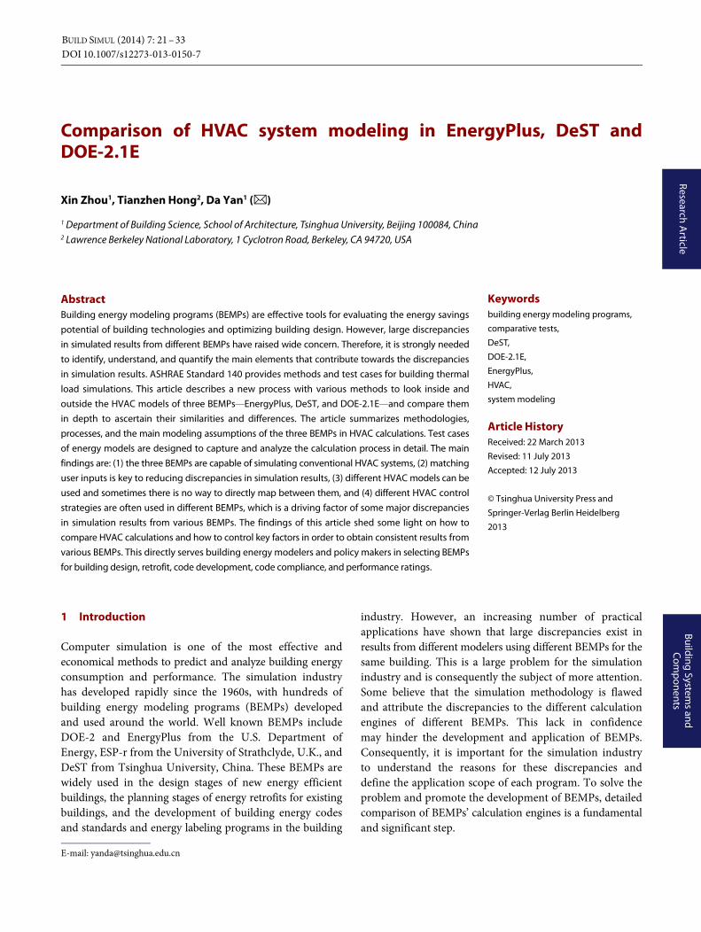
4.1.2 Building load calculation results

Using an outdoor air temperature of 10℃ as an example, the annual thermal loads for the five rooms from both programs are presented in Fig. 6. The loads calculated by the two simulation programs under the same outdoor air temperature are the same, so the differences arising from the HVAC system simulations can only be caused by the different calculation processes used on the HVAC side. By isolating the HAVC system from the load calculation, this method can focus on the principal problems, which is helpful to the analysis of the HVAC system calculation results. When the outdoor air temperature changes, various levels of building loads can be achieved. The building load will then be passed to the HVAC systems, so the calculation of operation strategies and equipment performance under different load ratios can be completed.

Fig. 5 The modified small office building

Table 4 Envelope constructions

Element External wall Interior wall Roof Floor

coefficient of heat transfer (W/(m2·K)) 0.694 2.573 1.274 4.249


28

Fig. 6 Annual load calculation results under an outdoor air temperature of 10℃ Note: ΔLoad = 2 × (DeST – EnergyPlus) / (DeST + EnergyPlus)

4.1.3 Test cases

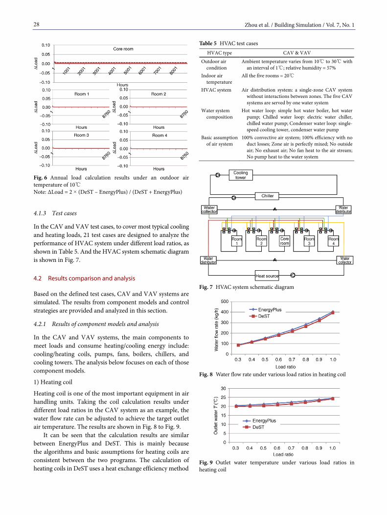
In the CAV and VAV test cases, to cover most typical cooling and heating loads, 21 test cases are designed to analyze the performance of HVAC system under different load ratios, as shown in Table 5. And the HVAC system schematic diagram is shown in Fig. 7.

4.2 Results comparison and analysis

Based on the defined test cases, CAV and VAV systems are simulated. The results from component models and control strategies are provided and analyzed in this section.

4.2.1 Results of component models and analysis

In the CAV and VAV systems, the main components to meet loads and consume heating/cooling energy include: cooling/heating coils, pumps, fans, boilers, chillers, and cooling towers. The analysis below focuses on each of those component models.

1) Heating coil

Heating coil is one of the most important equipment in air handling units. Taking the coil calculation results under different load ratios in the CAV system as an example, the water flow rate can be adjusted to achieve the target outlet air temperature. The results are shown in Fig. 8 to Fig. 9.

It can be seen that the calculation results are similar between EnergyPlus and DeST. This is mainly because the algorithms and basic assumptions for heating coils are consistent between the two programs. The calculation of heating coils in DeST uses a heat exchange efficiency method

Table 5 HVAC test cases HVAC type CAV & VAV

Outdoor air condition

Ambient temperature varies from 10℃ to 30℃ with an interval of 1℃; relative humidity = 57%

Indoor air temperature

All the five rooms = 20℃

HVAC system Air distribution system: a single-zone CAV system without interactions between zones. The five CAV systems are served by one water system

Water system composition

Hot water loop: simple hot water boiler, hot water pump; Chilled water loop: electric water chiller, chilled water pump; Condenser water loop: single- speed cooling tower, condenser water pump

Basic assumption of air system

100% convective air system; 100% efficiency with no duct losses; Zone air is perfectly mixed; No outside air; No exhaust air; No fan heat to the air stream; No pump heat to the water system

Fig. 7 HVAC system schematic diagram

Fig. 8 Water flow rate under various load ratios in heating coil

Fig. 9 Outlet water temperature under various load ratios in heating coil


29

(Jones 1985), while EnergyPlus uses the ε-NTU method (EnergyPlus 2011), but under heating load conditions, the two methods are equivalent.

2) Cooling coil

Similar with the comparison of heating coil, a CAV system is taken as an example to compare the calculation of cooling coil in DeST and EnergyPlus. In the two programs, the water flow rate in the cooling coil is adjustable to get the appropriate supply air temperature.

The calculation results are shown in Fig. 10 and Fig. 11. It can be found that the calculation results are similar between EnergyPlus and DeST. This is mainly because the algorithms and basic assumptions for cooling coils are consistent between the two programs. The heat exchange efficiency method is used in DeST for the calculation of cooling coils, while the ε-NTU method in EnergyPlus, but under sensible load conditions only, the two methods are equivalent.

3) Pump

All the water pumps in the test cases, such as hot water pumps, chilled water pumps and condenser water pumps, were constant speed. Taking the chilled water pump as an example, the calculation results are shown in Table 6. The power value of the constant speed pump is the same under all load ratios, so only one value is presented in Table 6.

It can be seen that the results of DeST equal those of EnergyPlus. The input parameters of the pump models in both programs, including rated flow rate, rated pump head

Fig. 10 Water flow rate under various load ratios in cooling coil

Fig. 11 Outlet water temperature under various load ratios in cooling coil

and pump efficiency, and the calculation equations are all the same. When flow rate changes, pump head and efficiency would be adjusted according to the flow rate ratio, and the modification equations are both quadratic curves for both programs.

One thing to note, is that in EnergyPlus, the total efficiency of pumps equals the product of the motor efficiency and the impeller efficiency. When a pump is auto-sized, the impeller efficiency is set to a value of 0.823 in the code, and the motor efficiency is entered by the user. In DeST, the input efficiency is the total efficiency.

4) Constant speed fan

The results for fan power with changing load ratio are shown in Table 7. Similarly, the power value of the constant speed fan is the same under all load ratios, so only one value is presented in Table 7. The results indicate almost no difference between the two programs. In DeST and EnergyPlus, the fan model uses the same equation. DeST assumes that the air density is a constant of 1.2 kg/m3, while in EnergyPlus, the air density is under standard conditions, which means that the local atmosphere has an air temperature of 20℃, and the humidity ratio is 0. Under normal conditions, the differences caused by the air density can be ignored.

5) Boiler

The simulation results for boilers, shown in Fig. 12, from both programs are similar. In both programs, the gas consumption of the boiler is a function of the heating load and the boiler’s efficiency. The boiler efficiency under part load conditions is calculated using a quadratic curve.

Table 6 Electric power of chilled water pumps EnergyPlus DeST

Power of chilled water pump (kW) 0.43 0.43

Table 7 Electric power of fans EnergyPlus DeST

Power of fans (kW) 499.76 502.31

Fig. 12 Gas power of boilers


30

6) Chiller

The calculation results from the chiller tests are shown in Fig. 13. As EnergyPlus and DeST use different performance curves, differences in electricity use are introduced.

Curve models are used in the two programs, and the chillers’ performance under different situations is adjusted according to the load ratio of the chillers, the chilled water outlet temperature and the condenser water inlet temperature. In EnergyPlus, three electric chiller models are available: an electric chiller model based on the fluid temperature difference; an electric chiller model based on the condenser inlet temperature; and an electric chiller model based on the condenser outlet temperature. In this case, the electric chiller model based on the fluid temperature differences (EnergyPlus 2011) was chosen, because this model has the same input parameters as the chiller model (Zhang et al. 2008) in DeST.

7) Cooling tower

The calculation results for the cooling tower tests are shown in Fig. 14 and Fig. 15. Figure 14 shows how the fan power of the cooling tower changes as the load ratio increases. Due to the different fan models, when the load ratio decreases, the fan power consumption in the two programs will differ gradually, as shown. Figure 15 demonstrates the relationship between the inlet/outlet water temperatures of cooling tower under various load ratios. The differences in cooling tower inlet/outlet water temperature are very small due to the

Fig. 13 Chiller electric power and COPs

Fig. 14 Cooling tower fan electricity use under various load ratios

Fig. 15 Cooling tower inlet/outlet water temperature under various PLRs

consistent algorithms for the cooling tower used by both programs. The main reason for the difference is that the calculation methods for enthalpy and the air temperature used for auto-sizing in DeST and EnergyPlus are not the same.

In DeST, the condenser inlet temperature (the cooling tower outlet temperature) is first assumed, and then cooling tower inlet water temperature is calculated iteratively. In EnergyPlus, it is assumed that the enthalpy of the moist air can be determined using the air wet-bulb temperature. The cooling tower calculations in EnergyPlus can be divided into steady-state calculations and actual condition calculations. The cooling tower steady-state calculation is the same as that used in DeST. Similarly, an iterative method is also used for steady-state conditions. The only differences are the initial assumptions for the cooling tower outlet air wet-bulb tem-perature and the convergence criteria. This methodology is


31

used to calculate the exiting water temperature in the free convection regime (water pump on, tower fan off) as well as when the tower fan operates, including low and high fan speed for the two-speed tower. Under actual conditions, the cooling tower model seeks to maintain the temperature of the water exiting the cooling tower at (or below) a setpoint specified by the user.

With regard to fan power calculations, DeST assumes a constant cooling tower fan power, while in EnergyPlus, the fan power is a linear interpolation of results from the two steady-state regimes—the tower fan switched on for the entire simulation time step and tower fan switched off for the entire time step.

4.2.2 Analysis of control strategies

The calculation results for the supply air temperature and supply air volume in a VAV system are compared to analyze the simulation of control strategies in EnergyPlus and DeST. As there are multiple control strategies for VAV systems in EnergyPlus, the control behavior corresponding to the Normal Acting damper for the terminal units is chosen. A Normal Acting damper means that during space heating, the damper stays at a minimal airflow position.

The calculation results for the supply air volume and supply air temperature are depicted graphically in Fig. 16 and Fig. 17, taking the core room as an example. A negative load ratio represents a cooling load. It can be seen that

Fig. 16 Supply air temperature and volume of the core room under specified control strategies

Fig. 17 Indoor air temperature of the core room under specified control strategies

supply air temperatures from both programs are almost the same, but there are discrepancies in supply air volume, which lead to inconsistent indoor air temperatures.

The calculation process used to determine the supply air temperature and supply air volume is different between EnergyPlus and DeST. In DeST, the supply air temperature and supply air volume are determined by an optimization algorithm, which ensures that, under the premise that the room setpoint can be reached, the air supply volume is set to the minimum possible rate. However, in EnergyPlus for normal acting dampers, when there is a heating load, the supply air volume is set to the minimum value, and the supply air temperature is determined by the load and the flow rate. In this case, when the heating load ratio is 1 (100% load), to maintain the room temperature setpoint, the supply air temperature can exceed the maximum value of 32℃. So the supply air temperature is set to 32℃ as Fig. 16 shows, and the room temperature is lower than the setpoint 20℃, as Fig. 17 shows, because it cannot meet the desired load. When a cooling load is required, the supply air temperature is determined first. It is a function of the room load and the flow rate from the previous time step. When the supply air temperature decreases to the lowest limit, the minimum value would be taken. The supply air volume is then determined from an energy balance calculation.

To verify this is due to the control strategy, the supply air temperature and supply air volume in EnergyPlus are set to the same as in DeST. This can be achieved by specifying the supply air temperature setpoint and the minimum supply air volume via the schedules. The results are shown in Fig. 18 and Fig. 19.

It can be seen that the supply air temperature and supply air volume are almost the same. Providing that the control strategies are set the same, the air systems perform consistently.


32

Fig. 18 Supply air temperature and volume of the core room under the same control strategy

Fig. 19 Indoor air temperature of the core room under the same control strategy

5 Conclusions

EnergyPlus, DeST, and DOE-2.1E have fundamental capabilities and appropriate modeling assumptions for HVAC system simulations. The results from the comparative tests on component models show small differences, which are mainly due to the user inputs and component algorithms used in each program. Differences between the total energy consumption of HVAC systems from DeST and EnergyPlus are within a 10% range, if all component models are chosen to be similar and the same or equivalent inputs for the HVAC systems are used. It is found that the main influencing factors on HVAC discrepancies between DeST

and EnergyPlus are the algorithms used for the HVAC component models and their control strategies.

EnergyPlus and DeST have comprehensive component models for users to select. The two programs have consistent models for pumps, fans, and boilers. The coil models in EnergyPlus and DeST are based on engineering equations, while the coil model in DOE-2 is based on empirical formulae. The elements that affect the chiller efficiency are consistent across the three programs, but the performance curve equations are not the same. In EnergyPlus and DOE- 2.1E, the fan power of the cooling tower is related to the load ratio—the fan can cycle during a particular time step if the load is small. In DeST, the fan power draw remains constant whenever the cooling tower has a load to meet for any hour. DOE-2 lacks the integrated solution of loads, systems, and plants, which is a serious limitation that makes it inappropriate for the simulation of complex HVAC systems or control strategies.

To complete a comprehensive comparison of the three simulation programs, several requirements are needed: (1) the test cases should be broad enough to cover most modeling features; (2) the test cases should be detailed enough to isolate influencing factors; (3) special cases should be designed to test the unique limitations of the programs. Based on the current development of HVAC system tests, a testing concept is introduced in this article to develop a better method for comparison. As each component in a HVAC system is connected and influenced by one another, the whole HVAC system should be considered when the comparison is conducted. This means that both air-side and plant-side components should be tested together. Imposing steady-state conditions makes it possible to compare each component model in detail and calculate analytical solutions. Considering the whole system makes the test process more practical.

The findings aim to shed some light on how to compare HVAC simulations between programs and how to control key factors in order to obtain consistent results and understand sources of discrepancies. This directly serves building energy modelers and policy makers in selecting appropriate programs for building design, retrofit, code development, code compliance, and performance ratings.

Acknowledgements

This study is supported by the International Science and Technology Cooperation Plan “U.S.-China Clean Energy Research Center for Building Energy Efficiency” (Grant No. 2010DFA72740-02) and “the 12th Five-Year” National Key Technology R&D Program of China (Grant No. 2012BAJ12B03). It was co-sponsored by the Energy Foundation under the China Sustainable Energy Program.


33

References

ANSI/ASHRAE (2007). ANSI/ASHRAE Standard 140-2007, Standard Method of Test for the Evaluation of Building Energy Analysis Computer Programs. Atlanta, GA, USA: American Society of Heating, Refrigerating and Air-Conditioning Engineers.

Crawley DB, Hand JW, Kummert M, Griffith BT (2008). Contrasting the capabilities of building energy performance simulation programs. Building and Environment, 43: 661 673.

DOE-2 (1982). DOE-2 Engineers Manual Version 2.1A, LBL-11353. DOE-2 (1993). DOE-2 BDL Summary Version 2.1E, LBL-34946. DOE-2 (1984). DOE-2 Supplement Version 2.1C, LBL-8706. Rev. 4.

Suppl. EnergyPlus (2011). Engineering Reference Version 7.0 Documentation.

University of Illinois and Ernest Orlando Lawrence Berkeley National Laboratory, USA.

Felsmann C (2008). Mechanical Equipment & Control Strategies for a Chilled Water and a Hot Water System. Available: http://archive.iea-shc.org/publications/downloads/task34-subtaskd. pdf. Accessed Jan. 2013.

Henninger RH, Witte MJ (2011a). EnergyPlus Testing with IEA BESTEST Mechanical Equipment & Control Strategies for a Chilled Water and a Hot Water System, EnergyPlus Version 7.2.0.006. Efficiency and Renewable Energy, Office of Building Technologies, U.S. Department of Energy. Available: http://apps1.eere.energy.gov/buildings/energyplus/pdfs/energyplus_ hvac_heat-cool-coil_tests.pdf. Accessed Jan. 2013.

Henninger RH, Witte MJ (2011b). EnergyPlus Testing with Global Energy Balance Tests, EnergyPlus Version 7.2.0.006. Efficiency and Renewable Energy, Office of Building Technologies, U.S. Department of Energy. Available: http://apps1.eere.energy.gov/ buildings/energyplus/pdfs/energyplus_hvac_global_tests.pdf. Accessed Jan. 2013.

Henninger RH, Witte MJ (2011c). EnergyPlus Testing with HVAC Equipment Performance Tests CE100 to CE200 from ANSI/ASHRAE Standard 140-2007, EnergyPlus Version 7.2.0.006. Efficiency and Renewable Energy, Office of Building Technologies, U.S. Department of Energy. Available: http://apps1.eere.energy.gov/ buildings/energyplus/pdfs/energyplus_ashrae_140_hvac_ce100to200. pdf. Accessed Jan. 2013.

Henninger RH, Witte MJ. (2011d). EnergyPlus Testing with HVAC Equipment Performance Tests CE300 to CE545 from ANSI/ ASHRAE Standard 140-2007, EnergyPlus Version 7.2.0.006. U.S. Department of Energy. Available: http://apps1.eere.energy.gov/ buildings/energyplus/pdfs/energyplus_ashrae_140_hvac_ce300to545.pdf. Accessed Jan. 2013.

Henninger RH, Witte MJ (2011e). EnergyPlus Testing with Fuel-Fired Furnace Tests HE100 to HE230 from ANSI/ASHRAE Standard 140-2007, EnergyPlus Version 7.2.0.006. Efficiency and Renewable Energy, Office of Building Technologies, U.S. Department of Energy. Available: http://apps1.eere.energy.gov/buildings/energyplus/ pdfs/energyplus_ashrae_140_hvac_he100to230.pdf. Accessed Jan. 2013.

Henninger RH, Witte MJ (2011f). EnergyPlus Testing with HVAC Equipment Component Tests, EnergyPlus Version 7.2.0.006. Efficiency and Renewable Energy, Office of Building Technologies, U.S. Department of Energy. Available: http://apps1.eere.energy.gov/ buildings/energyplus/pdfs/energyplus_hvac_component_tests.pdf. Accessed Jan. 2013.

Judkoff R, Neymark J (2006). Model validation and testing: The methodological foundation of ASHRAE Standard 140. Paper presented at the ASHRAE 2006 Annual Meeting, Quebec City, Canada.

Judkoff R, Neymark J (1995). International Energy Agency Building Energy Simulation Test (BESTEST) and Diagnostic Method. Available: http://www.nrel.gov/docs/legosti/old/6231.pdf. Accessed Jan. 2013.

Purdy J, Beausoleil-Morrison I (2003). Building Energy Simulation Test and Diagnostic Method for Heating, Ventilation, and Air-Conditioning Equipment Models (HVAC BESTEST): Fuel- Fired Furnace Test Cases. Available: http://archive.iea-shc.org/ publications/downloads/Furnace%20HVAC%20BESTEST%20Report.pdf. Accessed Jan. 2013.

Neymark J, Judkoff R (2002). International Energy Agency Building Energy Simulation Test and Diagnostic Method for Heating, Ventilating, and Air-Conditioning Equipment Models (HVAC BESTEST) Volume 1: Cases E100–E200. Available: http://www.nrel.gov/docs/fy02osti/30152.pdf. Accessed Jan. 2013.

Jones WP (1985). Air Conditioning Engineering. London: Edward Arnold.

Yan D, Xia J, Tang W, Song F, Zhang X, Jiang Y (2008). DeST—An integrated building simulation toolkit, Part I: Fundamentals. Building Simulation, 1: 95 110.

Yuill G, Haberl J (2002). Development of Accuracy Tests for Mechanical System Simulation, 865 TRP. Atlanta, GA: American Society of Heating, Refrigerating, and Air-Conditioning Engineers.

Zhang X, Xia J, Jiang Z, Huang J, Qin R, Zhang Y, Liu Y, Jiang Y (2008). DeST—An integrated building simulation toolkit, Part II: Applications. Building Simulation, 1: 193 209.

Zhu D, Yan D, Wang C, Hong T (2013). Comparison of building energy modeling programs: DeST, EnergyPlus and DOE-2. Building Simulation, 6: 323 335.

Documents

Comparison of HVAC system modeling in EnergyPlus, DeST and ... · In the integrated test cases part, based on the review of existing HVAC system tests, an integrated test method is