Comparison of optimal designs of steel portal frames includingtopological asymmetry considering rolled, fabricated and taperedsectionsMcKinstray, R., Lim, J. B. P., Tanyimboh, T. T., Phan, D. T., & Sha, W. (2016). Comparison of optimal designs ofsteel portal frames including topological asymmetry considering rolled, fabricated and tapered sections.Engineering Structures, 111, 505–524. https://doi.org/10.1016/j.engstruct.2015.12.028

Published in:Engineering Structures

Document Version:Peer reviewed version

Queen's University Belfast - Research Portal:Link to publication record in Queen's University Belfast Research Portal

Publisher rights© 2016 Elsevier Ltd. This manuscript version is made available under the CC-BY-NC-ND 4.0 license http://creativecommons.org/licenses/by-nc-nd/4.0/whichpermits distribution and reproduction for non-commercial purposes, provided the author and sourceare cited.

General rightsCopyright for the publications made accessible via the Queen's University Belfast Research Portal is retained by the author(s) and / or othercopyright owners and it is a condition of accessing these publications that users recognise and abide by the legal requirements associatedwith these rights.

Take down policyThe Research Portal is Queen's institutional repository that provides access to Queen's research output. Every effort has been made toensure that content in the Research Portal does not infringe any person's rights, or applicable UK laws. If you discover content in theResearch Portal that you believe breaches copyright or violates any law, please contact openaccess@qub.ac.uk.

Download date:02. Apr. 2020

1

Comparison of Optimal Designs of Steel Portal Frames Including Topological

Asymmetry Considering Rolled, Fabricated and Tapered Sections

Ross McKinstray, James B.P. Lim, Tiku T. Tanyimboh, Duoc T. Phan, Wei Sha*

*Corresponding author

Ross McKinstray: SPACE, David Keir Building, Queen's University, Belfast, BT9 5AG, UK.

James B.P. Lim: SPACE, David Keir Building, Queen's University, Belfast, BT9 5AG, UK.

Tiku T. Tanyimboh: Department of Civil and Environmental Engineering, University of

Strathclyde, James Weir Building, 75 Montrose Street, Glasgow, G1 1XJ, UK.

Duoc T. Phan: Department of Civil and Construction Engineering, Faculty of Engineering

and Science, The Curtin University Sarawak, Miri 98009, Malaysia.

Wei Sha: SPACE, David Keir Building, Queen's University, Belfast, BT9 5AG, UK. Email:

w.sha@qub.ac.uk

2

Comparison of Optimal Designs of Steel Portal Frames Including Topological

Asymmetry Considering Rolled, Fabricated and Tapered Sections

Abstract

A structural design optimisation has been carried out to allow for asymmetry and fully

tapered portal frames. The additional weight of an asymmetric structural shape was found to

be on average 5 to 13% with additional photovoltaic (PV) loading having a negligible effect

on the optimum design. It was also shown that fabricated and tapered frames achieved an

average percentage weight reduction of 9% and 11%, respectively, as compared to

comparable hot-rolled steel frames. When the deflection limits recommended by the Steel

Construction Institute were used, frames were shown to be deflection controlled with

industrial limits yielding up to 40% saving.

Keywords: Hot-rolled steel; Fabricated beams; Portal frames; Genetic algorithms;

Serviceability limits; Buckling limits

1 Introduction

For steel portal frames, a recent paper [1] has shown that asymmetric shapes with

photovoltaic (PV) panels on the southward side were advantageous for a low energy driven

design. Asymmetry and PV panels allowed for reduced embodied energy solutions (less

insulation) to achieve zero carbon standing by increased PV renewable space. The

increased degree of asymmetry was shown to be very useful for zero carbon building code

compliance where a calculated degree of asymmetry (from an energy simulation

optimisation) could be used to meet zero carbon requirements.

In another recent paper [2], a framework for a structural design optimisation for symmetrical

portal frames that used S275 steel was presented that considered frames from rolled

sections and frames from fabricated sections. This present paper now investigates the effect

3

of asymmetry [1] on the structural design optimisation with photovoltaic panels on the

southward side of weight 0.4 kN/m2. Two frame configurations are considered; symmetric

frames and asymmetric frames with an apex ratio of 0.8. Within the design optimisation, a

decoupled approach from the energy optimisation is taken with the main goal to establish the

effect of asymmetry on the optimisation. No attempt is made to link the structural design

optimisation to energy optimisation as it was shown that the steel weight would have an

insignificant effect on the energy design.

The frame constructions in this paper differ from those by McKinstray et al. [2] due to the

asymmetry and the additional tapered frame GA configurations case. Tapered frames [3], [4]

are the more efficient type of portal frame as these allow the cross-section to vary as

required [5] rather than being limited to a single critical ultimate limit state (ULS) load

position that would control a frame made from rolled or fabricated I sections. This present

paper investigates the structural effect of this asymmetry on the structural members. An

optimisation framework is described to design portal frames for minimum primary member

weights in accordance with the Eurocodes. Unlike [2], S355 steel is used as it has become

common practice to use this grade in portal frames due to its availability and similar price to

S275. Although it does not provide any benefits in terms of reducing deflections, the

additional yield strength can be useful in reducing buckling. For each of the construction

methods, a single optimisation configuration case is used (see Figure 1 and below);

C1 - Rolled I beam sections (selected from the Tata Steel bluebook [6]). This

configuration has 6 decision variables

C2 - Fabricated I sections (I beams fabricated from 3 plates). This configuration has 12

decision variables

C3 - Fully fabricated tapered frames (I beams fabricated from 3 plates but with varying

section depth). This configuration has 15 decision variables

4

As mentioned earlier, the addition of PV is accounted for through increased permanent

loading on the southward side, represented by an additional 0.4 kN/m2. In addition, the

effects of wind loading are added to the list of considered load combinations. Asymmetry

also increases the severity of a load occurring only on one side of the frame. To address

this, load combinations are considered with loads present on one side as well as both sides

of the roof. These result in 120 load combinations, including 28 serviceability limit state

(SLS) combinations (14 load combinations for differential deflection limit, 14 for absolute

deflection limit) and 92 ULS combinations. The deflection limits recommended by the Steel

Construction Institute (SCI) [7] are adopted; a comparison is also made to the less

conservative limits from the industry [8] in Section 2. The effects of the additional wind load

combinations beyond the gravity load combination used by McKinstray et al. [2] are

investigated in Section 2 also, for frame moments.

A wide range of topologies as well as different ranges of variable and permanent actions are

considered. The controlling load combinations were identified at positions through the frame

as well as the increase in moment at the column tops. It was found that wind loading can

increase maximum design moments in the column tops by a factor from 1 to 3, depending on

the span and column height.

A reference frame configuration is optimised, with a span of 35 m and column heights of 6

and 12 m (see Section 4). It is optimised for symmetric and asymmetric configurations with

apex ratios of 0.5 and 0.8 respectively [1]). The influence of the combination of wind loading,

PV loading and asymmetry on the primary steel mass for the reference frame is established.

It is shown that the SCI serviceability limits greatly control the design and that with deflection

limits the additional PV loading has a negligible effect on the optimum primary member

weight.

A topographical parametric study is then described (Section 5) covering different spans (14.5

to 50 m) and column heights (4 to 11.4 m) for different site locations (wind speeds) and

5

displacement limits (SCI and Industrial limits). Here, the effects of wind loading, asymmetry

and deflection limits are investigated. It was found that wind load has a significant effect on

the optimisation compared to just the gravity load combination. Tapered sections were found

to allow for additional weight savings (2-10% extra) compared to fabricated sections. The

effect of asymmetry is shown to be small with average weight increase of 4-13%, with the

smallest increase found in tapered frames followed by rolled sections and then fabricated

sections.

2 Limitsstatedesign

Modern practice has shown that plastic design produces the most efficient designs in the

majority of cases [9], [10]. Elastic design is still used, particularly when serviceability limit

state deflections will control frame design [8], [11], [12]. Phan et al. [8] and McKinstray et al.

[2] both demonstrated that if the deflection limits recommended by the SCI are adopted,

serviceability limit states control design. In addition, deep fabricated sections tend to be

incapable of fully utilising the material in the cross-section beyond the elastic modulus.

Additionally tapered sections are also generally not considered suitable for plastic design.

Therefore, elastic design is used here. A frame analysis program, written by the authors in

MATLAB, was used for the purpose of the elastic frame analysis. The internal forces,

namely, axial forces, shear forces, and bending moments can be calculated at any point

within the frame. The MATLAB program was capable of capturing the behaviour of tapered

members.

2.1 Frameloadingtypes

A number of load combinations [13] must be verified in the design of steel portal frames.

This is obtained through the rules for actions found in BS EN 1991 [14] and the rules for

combinations of actions in BS EN 1990 [15]. The combination of actions is the combination

of permanent, variable snow and wind actions on the structure multiplied by load factors

determined from the design code.

6

Permanent actions are the self-weight of the structure including primary steelwork, purlins

and secondary steel (0.1 kN/m2), cladding materials (0.2 kN/m2), building services (0.25

kN/m2) and photovoltaic panels and services (0.4 kN/m2). Permanent loads are determined

from the manufacturer’s specification and are identical to [2], apart from the additional PV

loading that is included on a single roof side. In addition, variable actions including access,

wind and snow are considered. Snow loading is calculated based on BS EN 1991-1-3 [16]

and its National Annex [17], assuming that a non-accidental case (drift) of 0.4 kN/m2 is

typical. Loads on roofs that are not accessible, except for normal maintenance and repair,

are classed under category H in BS EN 1991-1-1 [14]. For that category of roof, the UK

National Annex to BS EN 1991-1-1 [18] gives a variable loading of 0.6 kN/m2 for slopes

under 30o.

Wind actions are calculated according to BS EN 1991-1-4 general actions wind actions [19].

Four wind cases are considered based on 360 degree wind calculation method and an

additional 2 cases with wind direction reversed to account for the asymmetric shape. For

simplicity, no account is taken for the effect of asymmetry on the calculation of the wind

pressures on the frame. In asymmetric frames the loading calculated for an equivalent

symmetric frame is used. Additionally, the largest zone values are used instead of the

higher localised values. Table 1 outlines the assumptions used in the calculation of wind

forces on the building located in Belfast using the largest wind zones. Calculations are also

made for Liverpool and Birmingham, which are used later in Section 5.4. The peak velocity

pressure is dependent on the topography (span & column height). Due to the nature of the

code, Liverpool and Birmingham peak velocity pressures are scalable. For example if

Belfast had a dynamic wind pressure of 1.3 kN/m2, Liverpool and Birmingham would be 1.0

kN/m2 and 0.8 kN/m2, respectively.

2.2 Frameloadcombinations

Loads are factored together in accordance with EN1990 for ULS (Table 2). Equation 6.10

may be used solely as it is the most conservative of the three. For portal frames the benefits

7

of the more economical Equations 6.10a and 6.10b are generally not significant [12]. A

number of standard ULS combinations exist (Table 3) for the design of symmetric portal

frames [12] generated from Equation 6.10. When asymmetric frames are considered,

additional loading conditions need to be considered. For symmetric frames it is reasonable

to assume that the symmetric loading will produce the most onerous ULS combinations.

However, for asymmetric frames with significant degrees of asymmetry this is less likely,

making localised loading more significant. Examples include snow or access loading on a

single side of the frame. As will be shown later in the paper, no snow loading is not

considered as a dominate load case. Drive snow could be a topic of future research, but it

would need to exceed the imposed loading for it to be dominant. It is normal practice to

assume that there will be no imposed loading during storms or in snow conditions.

The addition of the photovoltaic panels adds loading to one side of the frame and so needs

to be considered in conjunction with the other load combinations, as well as the possibility of

the photovoltaic panels being removed. To account for the identified loading conditions the

standard ULS load combinations in Table 3 are expanded to include the asymmetric

conditions (Table 4). Combinations 1 and 2 in Table 3 are reduced to just combination 1 as

access load is the dominant of the two.

2.3 Importanceofadditionalwindloadcombinations

The additional load combinations (generated from the wind) can be visualised in an

exemplar 35 m span frame with 6 m column height and apex ratio of 0.7. Loading is

calculated as outlined in Section 2.1, with wind loading calculated for Belfast. Figure 2a

shows the bending moments for the analysis. Each green line indicates an individual load

combination (LC) bending moment diagram. The thick outer line shows the ULS condition for

all the combinations combined (bending moment envelope). The thicker blue line is load

combination LC1 (gravity load combination) for comparison. For this frame configuration

there are minor differences between the gravity load combination (LC1) and the additional

load combinations in terms of maximum moments or general moment shape.

8

When optimising tapered frames the point of contraflexure is important, as under a single

load combination this point will have zero bending moment. However, it was found from

Figure 2a that this effect of the point of contraflexure is not valid for design practice, since

significant bending moments are obtained from the other load combinations. If a small

number or the single gravity load combination was used in an optimisation, dangerously

small moments would be used in the verification of bending and buckling in the segment

surrounding the point of contraflexure.

Frames using rolled or fabricated I sections are not affected by the point of contraflexure

moving as the cross-section is constant across the frame, and is capable of carrying the

larger bending moment elsewhere successfully. This can make the additional load

combinations critical in controlling the minimum section size within the rafter for tapered

frames. Conservatively it is possible to base the design on the moment envelope (thick black

outer line) and not on a single load combination.

2.4 Serviceabilityandultimatelimitstatedesignrequirements

Serviceability deflection limits were calculated based on 14 differential and 14 absolute load

combinations, as seen in Table 5. Based on these load combinations, deflection limits

recommended by the SCI [7] or from industry [8] were adopted where stated (see Table 6).

Secondly, considering ultimate limit state design, structural members are designed to satisfy

the requirements for local capacity in accordance with Eurocode 3 [20]. Specifically,

members are verified for capacity under shear, axial, moment, and combined moment and

axial force. For fabricated and tapered beams, the buckling curves used are taken in

accordance with the UK National Annex [21]. The frame is split into a number of segments

(each with 5 nodes) between restraint positions. Each segment is then checked at each

node position for the maximum and minimum (reversed moment) ULS load combination (for

local capacity and buckling across the whole segment). This differs from [2] where buckling

was only evaluated at specified positions. Here, it is checked in every segment.

9

2.4.1 Shearcapacity

The shear force, VEd, should not be greater than the shear capacity, Vpl,Rd ;

RdplEd VV , (1)

The shear capacity is given by:

0

3,

M

yv

Rdpl

fA

V

(2)

where

fy is the yield stress of steel

Av is the shear area

0M is partial factor for resistance

2.4.2 Axialcapacity

The axial capacity should be verified to ensure that the axial force NEd does not exceed the

axial capacity (NRd) of the member.

RdEd NN (3)

2.4.3 MomentcapacityThe bending moment should not be larger than the moment capacity of the cross section,

Mpl,Rd.

RdplEd MM , (4)

where

MEd is the moment applied to the critical section

10

RdplM , is the moment capacity of the section.

Where members are subject to both compression and bending, the moment capacity RdplM ,

is reduced if the axial force is significant in accordance with clause 6.2.9 of Eurocode 3 Part

1-1 [20].

2.4.4 Buckling

The frame is split up into a series of segments between full restraints. Full restraints are

provided by ties joining the compression flange to secondary steelwork (purlins).

Irrespective of whether the frame is rolled, fabricated or tapered the segments are made

based on a 0.75 m and 1 m fixed spacing at the column tops, 3@1.5 m spacing at the eave,

and 1@1.5 m spacing at the apex (see Figure 3). Additionally a full restraint is provided at

any point where the tapered gradient changes (end of haunches). Outside of these fixed

spacing locations, full restraints are provided, with a maximum of 3 m in the columns and 4

m in the rafters.

Each segment is then verified based on the cross-sectional properties and individual

restraint spacing (at both ends of the segment). For segments where the cross-sectional

depth variation is less than 3%, buckling is verified using equations 6.61 and 6.62 of

Eurocode 3 [20]. Manufacturing tolerances of rolled beams is approximately 1% of the

height [22]. Over a segment length, height variations under 3% have more in common with

uniform beams rather than tapered sections. As the frame is under single axis bending the

additional second axis bending terms can be removed resulting in Equations 5 and 6 below

[12].

01,

,

,,

Rdb

Edyzy

Rdzb

Ed

M

Mk

N

N (5)

01,

,

,,

Rdb

Edyyy

Rdyb

Ed

M

Mk

N

N (6)

11

The equivalent uniform moment factors kzy and kyy (interaction factors) are calculated based

on the Annex B method of Eurocode 3 [20]. The maximum and minimum (reversed) bending

moments are both verified independently. The restraint spacing (Lcr) used in the calculation

of stability based unity factors is based on the bending moment. Where the bending moment

is positive with the bottom/internal flange in compression the segment length is used. This is

the distance between full restraints. When the moment is reversed and the bottom/internal

flange is in tension, the smaller of the maximum purlin spacing (1.5 m) or segment length is

used. No attempt is made to take advantage of any beneficial effect of restraints on the

tension flange. In-plane stability is verified using a buckling length of half the span,

irrespective of asymmetry within the frame.

For segments where the cross-sectional depth variation is more than 4% the segment is

verified using Equation 7 from NZS 3404:Part1:1997 Steel Structures Standard [23]. Design

element lengths are calculated in the same manner for uniform sections. The NZS 3404

method has been shown to be conservative for tapered sections [24] but does not need a

complex buckling analysis which would be infeasible for optimisation purposes. Other

possible methods for addressing stability, although not implemented here, include [25]–[27].

sxsxsmbx MMM (7)

where

αm is moment modification factor

αs is slenderness reduction factor

Msx is normal sectional moment capacity

Mbx is design sectional moment capacity.

12

2.5 IdentificationofcriticalULSloadcombinations

A study was conducted investigating 25600 frame configurations, based on the parameters

shown in Table 7, for each of the 92 ULS load combinations (Table 4). In each frame

configuration the critical or influential load combinations were recorded based on the

bending moment (at the level of the individual node). For the range of loading and building

shapes the maximum and minimum bending moments were recorded at each of the nodes

with the corresponding load LC value. Cross-section dimensions were based on optimum

design of symmetric portal frames using rolled sections [2]. Asymmetric frames were

assumed to have the same sections as the symmetric counterparts.

The frame was split into 4 quadrants: the 2 columns and the left and right rafters. Within

each quadrant, for both the maximum and minimum (reversed) bending moments the LC

identifier was recorded at each node. The number of occurrences that each load

combination controlled a node (in terms of % influence of all nodes in that quadrant) was

then reported (Table 8). A total of 33 unique ULS load combination cases were found to be

influential out of the possible 92 (≈36%). If only symmetric frames are considered the

number of influential load combinations drops to 30. The frame asymmetry shape caused

additional influencing combinations for the frame geometry. The majority of influential load

combinations occur in the left hand side of the frame where the maximum bending moment

and the minimum (reversed) bending moment occurred. The remainder of the quadrants

were influenced by under 5 load combinations.

A key observation in the study was the large variations in the distances between the more

traditional ULS gravity load combination LC1 and in some cases with wind included. In the

previous example (seen in Figure 2a), the variation between the envelope and the ULS

gravity combination LC1 (blue line) is small but this is not always the case (see Figure 2b).

The wind forces are large in comparison to the other actions, in frames with relatively high

column heights to span ratio. Here, the wind forces are larger and have more influence,

leading to much larger moments as compared to the gravity load combination.

13

The influence of the wind on the ULS moments compared to the gravity load combination

was calculated for the range of building configurations by comparing the maximum moment

at the column top between the wind load combinations (LC9-92) and the gravity load

combination (LC1). The ratios are reported in Figure 4 for symmetric frames. It can be seen

that for frames with long span and short columns, higher wind has very little influence on the

ULS design of the frame. However, there is an exponential increase in the influence of the

wind for short frames with high column heights.

This increase in moment can be very significant conceivably requiring considerably larger

sections to carry the increased moments. This would call into question the validity of gravity

load combination based optimisation as any result could be misleading requiring larger

sections than would be expected. Particularly, most frames are deflection controlled which

allows for some additional moment carrying capacity. However, the wind load combinations

will also increase the deflections resulting in inevitable larger sections as there will be no

additional deflection capacity in optimum designs.

3 GAoptimisation

3.1 Optimisationmodel

The objective of the overall design optimisation is to determine the steel frame with the

minimum primary member steel material weight, whilst satisfying the design requirements.

Previous optimisation research has been carried out for steel frames and truss structures

[28]–[32] but not on portal frames with asymmetry and tapering. The weight of the frame

depends on the cross-section sizes of members. The objective function is expressed in

terms of the weight of the primary members per square metre of the floor area. The weight

was based on the summation of the volume of steel material throughout the frame.

The unity factors and geometric limits for design constraints are as follows.

14

(1) For each segment:

1,

1 Rdpl

Ed

V

Vg (8a)

1,

2 Rdpl

Ed

V

Vg (8b)

13 Rd

Ed

N

Ng (8c)

1,

4 Rdpl

Ed

M

Mg (8d)

(2) For segments with uniform section profile:

1,

,

,,5

Rdb

Edyzy

Rdzb

Ed

M

Mk

N

Ng (8e)

1,

,

,,6

Rdb

Edyyy

Rdyb

Ed

M

Mk

N

Ng (8f)

(3) For segments with tapered section profile:

165 bx

Ed

M

Mgg (8g)

(4) Whole frame displacements:

17 ue

eg

(8h)

18 ua

ag

(8i)

(5) Geometric limits:

Otherwise0

3 if2.19

htg f (8j)

Otherwise0

if2.110

fw ttg (8k)

15

The notations are standard for the Eurocodes, where the same notation is used for both

shear capacity and shear buckling capacity. The constraints for ultimate limit state design

are g1 to g6 while the serviceability limit state design constraints are g7 and g8. Constraint g1

is for shear capacity; g2 is for shear buckling; g3 is for axial capacity; g4 is for combined axial

and bending capacity; g5 and g6 are interaction of axial force and bending moment on

buckling for major axis; and g7 and g8 are for horizontal and vertical deflection limits. δe and

δa are deflections at eaves and apex, respectively. The superscript u indicates the maximum

permissible deflection. If the geometrical cross-section constraints g9 and g10 are exceeded,

an arbitrary (lowest tier) unity factor of 1.2 is assigned. These are verified throughout the

frame and are further denoted to show the maximum value within a given zone: gxC within the

column; gxR within the rafter; gxH within the haunch. Second order effects are not accounted

for in the scope of this paper as McKinstray [33] demonstrated that second order effects are

insignificant due to deflection limits controlling the design resulting in low axial forces and

therefore small second order effects [34].

3.2 Optimisationmethodology

The design optimisation considered in this paper contains mixed discrete and continuous

design variables. This was implemented using a genetic algorithm within the optimisation

toolbox in MATLAB, i.e., using standard routines. In order to consider discrete and

continuous design variables, special crossover and mutation functions enforce variables to

be integers [35]. It has been observed that using the real coded genetic algorithms, large

population sizes are needed in order to obtain the optimum solution consistently [36]. To

help improve computational efficiency and reliability, solution space reduction and enhanced

exploration based on larger initial populations, respectively, are employed here as in [2].

The three GA configurations are shown in Figure 1 and Table 9; C1 rolled frame optimisation

(6 variables), C2 fabricated frame (12 variables) and C3 tapered frame (15 variables). To

allow for asymmetry and for the increased loading on the PV side, the left and right sides of

the frames were able to vary independently. Otherwise the optimisation is similar to [2]. The

16

objective of the optimisation is to obtain the minimum weight of the primary members of the

portal frame. This includes the weight of the column, rafter and haunch elements. For the

haunch sections, this weight includes any wastage in material as a result of the fabrication.

The haunch sections are cut within the web outside the root radius, realistically reflecting

fabrication cutting conditions.

To solve the optimisation problem, a penalty was added to the achieved frame weight Fweight.

Equation 9 shows the fitness function Fp with two penalty levels. The constraint violation

penalty multiplier parameter P was the weight of the heaviest feasible configuration solution

based on the design optimisation constraints. Thus the penalty for moderate constraint

violations was P while larger violations incur a much larger penalty of 10P based on the

maximum value gM of any individual unity factor [33].

5.1 if10

5.11 if

1 if

Mweight

Mweight

Mweight

p

gPF

gPF

gF

F (9)

The penalty function in Equation 9 allows relatively small constraint violations to permit

searches in both the feasible and infeasible regions simultaneously. This is known to

improve the efficiency i.e. speed of the optimisation. It also prevents premature convergence

due to excessive and rapid loss of useful genetic material carried by infeasible solutions.

Table 9 gives a summary of the GA parameters. The crossover probability was 0.8.

Intermediate crossover and adaptive feasible mutation [37] were employed along with binary

tournament selection. The optimisation was conducted on a workstation (2.53 GHz CPU, 16

GB RAM). Individual fitness function evaluation calls took approximately one second for a

full solution. However, much faster solutions were possible if a dimensional check was

violated prior to analysis. Typical single optimisation run for C1, C2 and C3 are 20, 40 and

180 minutes respectively for 30 m span 6 m column height symmetric frame. The CPU

times seem reasonable.

17

The fitness function in Equation 9 combines the minimum weight and the constraint

violations. Progress of the genetic algorithm is determined by the fitness function. The best

solutions have the smallest constraint violations or none and the smallest weights. The

search is therefore driven by all the relevant design variables including weight and all

relevant design considerations i.e. Equations 1-9.

It should be noted that a minimum weight optimisation will not yield the same solution as a

minimum cost optimisation. However, the cost calculations are not included in this paper, to

limit the scope and the length of the paper.

4 Referenceframeoptimisation

The reference frame consists of a 30 m span frame with two column heights of 6 m and 12

m. Symmetric (apex ratio 0.5) and asymmetric (apex ratio 0.8) frames are considered. The

frame is optimised for the range of ULS and SLS loading combinations with serviceability

deflection constraints. From the optimisation the critical controlling factors in the design are

identified along with the effect of different configurations on the optimum weight. For the

reference frame and the 3 different GA configurations, different global population sizes were

investigated using a population based on multipliers of 1, 2, 4, 8 and 16 times the number of

decision variables with each optimisation run 20 times. The minimum weight and standard

deviation for the 20 runs are recorded in Table 10.

As can be seen from Table 10, the reduction in standard deviation caused by increasing the

population size has reached a point of diminishing returns. The standard deviations of the

optimised weights are practically zero as shown in Table 10. In other words the GA finds

optimal and near optimal solutions consistently. The population sizes used depend on the

number of decision variable and multipliers of 8 to 16 were used. This is fairly typical and

consistent with standard practice. Search space reduction eliminates portions of the solution

space with infeasible and/or extremely expensive solutions. Finally the expanded initial

population achieves much greater exploration early on in the optimisation. For faster

18

optimisation the number of runs is reduced to 8 rather than 20 runs. As the study covers

only a small topographical range of frame geometries it is advisable to choose conservative

values as frames with significantly different topography will be governed by different factors

leading to variable GA reliability and performance. Search space reduction and increased

initial population strategies were employed to enhance GA reliability further in all cases [2].

4.1 Referenceframeoptimisationstudyoutline

The reference frame was optimised under a range of loading and constraint configurations.

Three sets of displacement limits were considered:

(1) none ‒ with no SLS limits

(2) SCI ‒ where the SCI limits are used

(3) IND ‒ where the industry limits are used

Each frame was checked independently using ULS combinations LC1-8 and the full set of

ULS combinations LC1-92. ULS combinations LC1-8 exclude the wind loading and closely

resemble the previous works that excluded wind loading combinations that make up load

combinations LC9-92. Additionally, the frames were considered with and without PV loading

on the left (larger) side of the frame.

Table 11 shows the optimum frame weights for 144 frame configurations. Each solution is

based on 8 optimisation runs with the minimum weight and standard deviation reported. It

can be seen that in general terms, C1 produces the heaviest frames, C3 the lightest, and C2

in between as would be expected. In comparison to the minimum weight, the standard

deviations are small for most cases, which indicates that the GA is well performing. The

standard deviation in the table can be quite high for some optimisation cases, mainly on the

fringes of the optimisation space (maximum column height 12 m). This primarily occurred

due to a single optimisation returning a local optimum weight, which would be larger than the

true optimum. However due to the 8 runs the effect of this single local optimum is small.

This was identified during the optimisation process and the number of runs was increased

19

from 6 to 8. The largest deviations occur in the heavier frames where a standard deviation

of 10 for a 100 kg/m2 frame has the same relative effect as deviation of 1 for a 10 kg/m2

frame. Taking this into account the variation across the table is relatively consistent

although with slightly poorer performance for 12 m column high frames with multiple

constraints (deflection limits).

From Table 11 a comparison can be made between the weight of symmetric and asymmetric

frames (Table 12). The frame weight increase caused by asymmetry is smaller than 20%,

i.e. not excessive. In some configurations the increase is smaller than 5%. In some cases

weight reductions are observed that could be attributed to either local optima or due to the

change in bending moment shape allowing for lighter solutions. Due to the relatively small

savings within the range of the standard deviations it is not possible to determine which is

more likely.

Table 13 shows the percentage increase in frame weight after adding PV loading to the

frame. Frames with no serviceability deflection limits have the highest increases in frame

mass. This is due to the frame being governed primarily by bending, resulting in mass

increases with any increase in loading. For frames with serviceability deflection limits in

place, the impact of the PV panels is minimal in most cases and within the standard

deviation of the optimum. This can be attributed to the frames being primarily governed by

the SLS deflection limits and is reflected in low unity factors for bending and axial force. As

the PV loading is small, only small amounts of additional deflection would be expected,

resulting in very small section size increases. In some cases, small (< 2%) weight savings

were observed; generally inside the standard deviation and indicative of the optimisation

being relatively consistent.

For this frame configuration the weight increases going from the first 8 ULS load

combinations to the full set are shown in Table 14. The largest weight increase can be seen

in frames without deflection control. This indicates that these frames are heavily controlled

20

by the wind loading, with frames with higher column heights having significantly large mass

increases. For frames with deflection controls, in all cases the weight increases are

relatively small (up to 10%). From Figure 4, the column top moment increases from the

gravity load combination to the full (92) ULS load combinations. For example, the moment

increase ratio is 1.2 and 1.8 for the 6 m and 12 m column heights frames, respectively. This

indicates that in this case the frame is mostly controlled by the serviceability deflection limits

with the additional bending moments added by the wind loading not affecting the final

weight, even with a significant 1.8 times increase in maximum column top moment.

4.2 Optimisationframeprofilecomparison

In conventional design, it is common practice to develop designs initially based on the

gravity load combination of the frame. Based on the bending moment diagram of the gravity

load combination, the frame is arranged into a series of elements, with additional steel in the

form of haunches or taper elements in the eaves where the moments are highest. It has

been shown previously that the inclusion of the wind adds a significant number of additional

bending moment diagrams that can have control over different parts of the structure.

Additionally, the displacement limits have been shown to be very influential in the selection

of section profiles controlling the design of the frames. For the reference frame with PV

loading, the frame profile is drawn for frames with SCI and without displacement limits

(Figure 5). The bending moment profile envelopes of all the ULS combinations are shown

on top of the frame profile to scale.

It can be seen that without SLS combinations the GA is producing generally conventional

frame shapes that to a good extent follow the bending moment shape. The addition of the

SLS combinations generally increases the size of the haunches without changing the overall

frame shape or configuration. The only exception is found in asymmetric frames where the

shorter rafter may deviate from the bending moment gradient.

21

The fully tapered framed shape (Figure 1c) has been significantly reconfigured by the GA

towards a more conventional haunched profile with only very minor taper to the rafter mid

span. This is attributable to the bending moment envelope being significantly different from

the idealised UDL gravity load combination that the shape is based upon. Unlike the more

traditional hatched portal frame, the tapered frame shape is unable to accommodate the

multiple moment diagrams created by different load combinations.

5 Parametricstudy

5.1 Configuration

In the previous section a single frame was investigated over a range of loading and

serviceability deflection limits. In this section, the weight across the range of standard portal

topographical configurations (spans/column heights) is optimised. Spans considered in the

study range from 14.5 m to 50 m; column heights range from 4 m to 11.5 m using S355

steel. The pitch and frame spacing for all frames are 10o and 6 m (used in typical

structures), respectively, resulting in a grid of 13×6 data points (highlighted in the contour

plots by dots). Both symmetric and asymmetric (0.8 apex ratio) frames are considered

separately using C1, C2 and C3 configurations. The optimum designs for the frames in this

section are obtained by running 8 optimisations per data point. For each combination, the

minimum weight was obtained (in terms of kg/m2) and reported within contours.

5.2 InitialstudywithSCIserviceabilitydeflectionlimits

Using the SCI serviceability deflection limits the optimised results for both symmetric and

asymmetric frames are presented in Figure 6 for rolled, fabricated, and tapered frames. It is

immediately clear that the profile of the contours differs significantly from those previously

reported by Phan et al. [8] and McKinstray et al. [2] where a monotonic trend was observed.

Excluding the wind load combinations, the same monotonic trend is found as in the literature

when using S355 steel (see Figure 7). This indicates that the wind load combinations have

22

a significant influence over the design resulting in heavier frames, in some cases. It should

be noted that the previous comparisons both used S275 steel and in Phan et al. [8] case

only rolled sections were considered. Figure 8 shows typical optimisation histories, for

symmetric 30 m span 6 m column height frames, to illustrate the progress of the

optimisation. The figure shows the number of function evaluations in each case.

A comparison between the optimisation solutions for different frame types is presented in

Figure 9. As would be expected, the rolled sections (C1) produce the heaviest frames

requiring the same weight for shorter span, shorter column height structures. For an equal

weight a larger structure could be designed using fabricated (C2) and even more so tapered

(C3) compared to rolled (C1) design. The new contour shape for frame resembles an ‘L’.

For the part parallel to the span axis the variation in weight between the methods is relatively

constant. However, for heavier frames, significantly larger savings are shown on the L leg.

This is an indication of the increased benefit of tapered frames in these situations over the

other configurations.

Figure 10 shows the weight reduction moving from rolled to fabricated, fabricated to tapered

and the overall reduction from rolled to tapered as a histogram of percentage reduction in

weight calculated from Figure 6. In general terms, tapered frames produce the lightest

results, followed by fabricated and then rolled frames. For symmetric frames the largest

savings on average (9%) are seen in moving from rolled to fabricated frames, with only a 2%

further reduction going from fabricated to tapered frames. For asymmetric frames the

reduction in optimum weight moving from rolled to fabricated sections is smaller (6%) with a

much larger reduction (10%) going from fabricated to tapered. For symmetric frames the

additional effort in the design and manufacturing of tapered frames is hard to justify due to

the small additional weight saving over fabricated frames. However, for asymmetric frames,

tapered frames have a significant benefit, with fabricated frames only having a small weight

reduction and the largest weight saving achieved through tapered geometry.

23

5.3 EffectofAsymmetry

Asymmetry does not change the overall trend or shape of the optimum contours (Figure 6).

It does however change the optimum weight. Figure 11 shows symmetric contours for C1, 2

and 3 overlapped with their asymmetric counterparts and histogram analysis of the weight

change. Asymmetry adds weight to the frame on average 9% for rolled frames, 13% for

fabricated frames and 5% for tapered frames. The maximum weight increase observed was

35%, found in both fabricated and rolled frames.

The largest increases in frame weight can be seen from the overlapping contours to occur in

long span frames with short column. This is attributed to SLS lateral displacement control of

the frames, for which a symmetric configuration can resist lateral deflection (especially to

short column) more effectively than the asymmetric one. Also, for long span and short

column, the moment difference at the critical section for asymmetric frames is larger than in

symmetric one. Fully tapered frames show much better adaptability to asymmetry than their

rolled and fabricated counterparts. The asymmetry contours can be seen to follow the

symmetric counterpart much closer including in the long span short column height scenarios.

The rolled and fabricated histograms could be described as skewed towards 5-10%; in

contrast the tapered frame has a more normal distribution around the same range. This

results in a number of topographies having no weight increase with a small number (<5%)

having a weight reduction for the tapered frame.

5.4 Importanceofthewindpressure

It has previously been shown that wind has a significant influence on the resulting contour

plot shape. However, this particular case examined Belfast, an area of the UK with relatively

harsh wind weather conditions. For the design proposed, wind speeds for the UK are

obtained from the National Annex of Eurocode 1 part 1-4 [38]. Belfast has an equivalent

wind speed of the Scottish lowlands. England has significantly lower wind speeds. Due to

the nature of the wind code it is possible to scale the wind loadings to obtain different

24

locations allowing for a fast rerunning of the optimisation without additional programming.

This was done for Liverpool (wind speed 23 m/s, peak velocity pressure 1.0 kN/m2) and

Birmingham (21.75 m/s and 0.787 kN/m2). The study was limited to C2 fabricated beams,

with SCI deflection limits for both symmetric (0.5 apex ratio) and asymmetric (0.8 apex ratio)

frames.

Comparing the no wind case to the 3 chosen locations for symmetric frames, Figure 12 plots

the percentage difference of the no wind case (Figure 7). In contrast to the reference frame,

wind can be seen to clearly dominate the design with its influences being very dependent on

the topographical configuration of the building. It is clear that for all Belfast and Liverpool

span/column height configurations, wind dominates the design adding at least 20% and 5%

to the design weights, respectively. Both locations have a large flat area with the minimum

percentage influence mainly for short column height building or for taller buildings with long

spans. Outside of this area there are significant weight increases based on the column

height to span ratio. Birmingham is the exception where the flat area is not dominated by

the influence of wind. However, like the other locations outside of this area wind dominates

the frame. Plotting the diagonal of the 3 locations (red dashed line) it can be seen that there

is a close relationship between the different locations, with higher wind load linearly

increasing the weight of the frame with similar exponential increases in frame weight based

on column high to span ratio.

The contours of frame weight for symmetric and asymmetric frames are shown in Figure 13

and Figure 14, respectively, together with histograms showing the percentage change in

weights compared to Belfast. It can be seen that the symmetric and asymmetric contour

plots follow each other well for each of the locations. By comparing the percentage variation

between each location and Belfast, a nearly normal distribution can be seen in each case.

This indicates that the weight difference between locations can be scaled, allowing for the

approximate calculation of optimum weights for any part of the UK (providing the scale factor

is known).

25

5.5 Effectofserviceabilitydeflectionlimits

For the three geographical locations the frames were re-optimised using the Industrial

deflection limits (Section 2.4). The frame weights in comparison to the SCI weight are

shown for Belfast in Figure 15, Liverpool in Figure 16 and Birmingham in Figure 17. A

similar L shaped contour plot pattern is observed in the frames with industrial deflection

limits as observed with SCI limits. For all locations a small area of frames with short column

height coupled with short spans were unaffected by the industrial deflection limits. Outside

of this configuration, using industrial limits can lead to weight saving of up to 40%.

The largest savings were found in frames with very tall column heights. For typical span to

column height ratio frames, saving of 15-30% primary member weight are realistically

achievable.

6 Conclusion

A structural design optimisation has been carried out to allow for asymmetry and fully

tapered portal frames. Universal beam sections, fabricated sections and tapered frames

were considered. Tapered frames were shown to produce the lightest solution followed by

fabricated and then rolled frames. However, for symmetric frames the weight savings are

small, with tapered frames only having a slight weight advantage over fabricated frames. As

a fabricated design is cheaper to implement, due to easier design and manufacturing,

tapered frames would struggle to be economically viable. For asymmetric frames the

opposite is true, with the largest weight saving found using tapered geometry and only minor

weight saving with fabricated sections. This makes tapered frames a much more viable

design solution. It was found that multiple load cases must be considered for the design of

tapered frames, particularly at the point of contraflexure where the additional bending

moments from the additional load combinations are accounted for in the design verification.

The traditional tapered frame shape is based on a single load combination (the gravity load

26

combination); however, the optimised results show little resemblance favouring a more

uniform profile with a slight taper.

In frames with SCI or industrial deflection limits, the addition of PV panels was shown to

have a minimal impact on the optimum weight. In contrast, wind has been shown to have a

significant influence on the resulting frame and should be included in the optimisation in

order to produce the most realistic results for design purposes. Wind increased bending

moment in frames (in some cases, very significantly), resulting in very different weight

contour profiles. The contour profiles were in stark contrast to gravity load combination

contours moving from a well-documented monotonic trend to an L shaped profile with a

significant horizontal weight profile. Weight increases were largest for Belfast with the

highest wind speed, and lowest for Birmingham with the slowest wind speed. For all

locations short column short span frames have a plateau area where the weight increases

due to wind is constant. For Birmingham no weight increases were observed in this area

(0%), Liverpool 5% and Belfast 20%. Outside of the area there is large increase in weight.

It was found that the optimal weight between the locations scaled well, indicating that weight

could be interpolated based on site wind speed, as based on the presented results.

Asymmetric frames weighed more than their geometrically similar symmetric counterparts.

Tapered frames had the smallest average weight increase of 5%, with fabricated sections

13% and rolled sections 9%. Tapered frame weight increases were also more consistent,

with a maximum increase of 15%, whereas for fabricated and rolled sections this could be as

high as 40%.

The chosen set of serviceability deflection limits has a significant impact on the frame

weight, with up to 40% saving achieved using the industrial serviceability deflection limits

compared to the SCI recommended limits. The weight saving is independent of the site wind

speed: with the three locations having similar contours with savings based on the

topographical configuration of the building. No savings were observed for very short column

27

height and span buildings, with the largest saving in very tall, but not necessarily long span

buildings.

References

[1] R. McKinstray, J. B. P. Lim, T. T. Tanyimboh, D. T. Phan, W. Sha, and A. E. I. Brownlee, “Topographical optimisation of single-storey non-domestic steel framed buildings using photovoltaic panels for net-zero carbon impact,” Build. Environ., vol. 86, pp. 120–131, 2015.

[2] R. McKinstray, J. B. P. Lim, T. T. Tanyimboh, D. T. Phan, and W. Sha, “Optimal design of long-span steel portal frames using fabricated beams,” J. Constr. Steel Res., vol. 104, pp. 104–114, 2015.

[3] H. Saffari, R. Rahgozar, and R. Jahanshahi, “An efficient method for computation of effective length factor of columns in a steel gabled frame with tapered members,” J. Constr. Steel Res., vol. 64, no. 4, pp. 400–406, Apr. 2008.

[4] M. Saka, “Optimum design of steel frames with tapered members,” Comput. Struct., vol. 63, no. 4, pp. 798–811, 1997.

[5] D. Fraser, “Design of tapered member portal frames,” J. Constr. Steel Res., vol. 3, no. 1, pp. 20–26, 1983.

[6] Tata Steel, Steel building design: design data. The Steel Construction Institute and The British Constructional Steelwork Association Limited, 2011.

[7] Steel Construction Institute, “SCI advisory desk AD 090: deflection limits for pitched roof portal frames (amended),” 2010.

[8] D. T. Phan, J. B. P. Lim, T. T. Tanyimboh, R. M. Lawson, Y. Xu, S. Martin, and W. Sha, “Effect of serviceability limits on optimal design of steel portal frames,” J. Constr. Steel Res., vol. 86, pp. 74–84, Jul. 2013.

[9] P. R. Salter, A. S. Malik, and C. M. King, Design of single-span steel portal frames to BS 5950-1:2000 (P252). Berkshire: The Steel Construction Institute, 2004.

[10] J. M. Davies and B. A. Brown, Plastic design to BS 5950. Berkshire: Steel Construction Institute, 1996.

[11] J. B. P. Lim and D. A. Nethercot, “Serviceability design of a cold-formed steel portal frame having semi-rigid joints,” Steel Compos. Struct., vol. 3, pp. 451–474, 2003.

28

[12] D. M. Koschmidder and D. G. Brown, Elastic design of single-span steel portal frame buildings to Eurocode 3 (P397). Berkshire: The Steel Construction Institute, 2012.

[13] S. K. Azad and O. Hasançebi, “Discrete sizing optimization of steel trusses under multiple displacement constraints and load cases using guided stochastic search technique,” Adv. Eng. Softw., vol. 52, no. 2, pp. 383–404, 2015.

[14] British Standards, BS EN 1991-1-1:2002; Eurocode 1: Actions on structures; Part 1-1: General actions - Densities, self-weight, imposed loads for buildings. London, UK, 2002.

[15] British Standards, BS EN 1990:2002; Eurocode: Basis of structural design (incorporating corrigendum December 2008 and April 2010). London, UK, 2002.

[16] British Standards, BS EN 1991-1-3:2003; Eurocode 1: Actions on structures. General actions - Snow loads (incorporating corrigenda December 2004 and March 2009). London, UK, 2003.

[17] British Standards, NA to BS EN 1991-1-3:2003 National Annex to Eurocode 1: Actions on structures. General actions - Snow loads (incorporating corrigendum no. 1, June 2007). London, UK, 2005.

[18] British Standards, NA to BS EN 1991-1-1:2002; UK National Annex to Eurocode 1: Actions on structures. General actions - Densities, self- weight, imposed loads for buildings. London, UK, 2005.

[19] British Standards, BS EN 1991-1-4:2005; Eurocode 1: Actions on structures Part 1-4: General actions Wind actions. London, UK, 2005.

[20] British Standards, BS EN 1993-1-1:2005; Eurocode 3: Design of steel structures Part 1-1: General rules and rules for buildings. London, UK, 2005.

[21] British Standards, NA to BS EN 1993-1-1: UK national annex to Eurocode 3: Design of steel structures. London, UK, 2005.

[22] British Standards, BS EN 10034:1993; Structural steel I and H sections tolerances on shape and dimensions. London, UK, 1993.

[23] Standards New Zealand, NZS 3404; Steel structures standard; Both parts supersede NZS 3404: Parts 1 and 2. New Zealand, 1997.

[24] M. Bradford and P. Cuk, “Elastic buckling of tapered monosymmetric I-beams,” ASCE J. Struct. Eng, vol. 114, no. 5, pp. 977–996, 1988.

[25] V. Šapalas, M. Samofalov, and V. Šaraškinas, “FEM stability analysis of tapered beam columns,” J. Civ. Eng. Manag., vol. 11, no. 3, pp. 211–216, Jan. 2005.

29

[26] L. Zhang and G. S. Tong, “Lateral buckling of web-tapered I-beams: A new theory,” J. Constr. Steel Res., vol. 64, no. 12, pp. 1379–1393, Dec. 2008.

[27] L. R. S. Marques, “Tapered steel members: flexural and lateral-torsional buckling,” PhD thesis, Universidade de Coimbra, 2012.

[28] S. K. Azad and O. Hasançebi, “Computationally efficient discrete sizing of steel frames via guided stochastic search heuristic,” Comput. Struct., vol. 156, pp. 12–28, Aug. 2015.

[29] M. R. Maheri and M. M. Narimani, “An enhanced harmony search algorithm for optimum design of side sway steel frames,” Comput. Struct, vol. 140, pp. 55–65, 2014.

[30] F. Flager, G. Soremekun, A. Adya, J. Kristina Shea, O. Haymaker, and M. Fischer, “Fully constrained design: A general and scalable method for discrete member sizing optimization of steel truss structures,” Comput. Struct., vol. 140, pp. 55–65, Jul. 2014.

[31] J. Leng, Z. Li, J. K. Guest, and B. W. Schafer, “Shape optimization of cold-formed steel columns with fabrication and geometric end-use constraints,” Thin-Walled Struct., vol. 85, pp. 271–290, 2014.

[32] M. Moharrami, A. Louhghalam, and M. Tootkabon, “Optimal folding of cold formed steel cross sections under compression,” Thin-Walled Struct., vol. 76, pp. 145–156, 2014.

[33] R. Mckinstray, “Single storey steel building optimisation for steel weight and carbon incorporating asymmetric topology with photovoltaic panels,” PhD thesis, Queen’s Univeristy Belfast, 2015.

[34] J. B. P. Lim, C. M. King, A. J. Rathbone, J. M. Davies, and V. Edmonson, “Eurocode 3 and the in-plane stability of portal frames,” Struct. Eng., vol. 83, no. 21, pp. 43–49, 2005.

[35] K. Deep, K. P. Singh, M. L. Kansal, and C. Mohan, “A real coded genetic algorithm for solving integer and mixed integer optimization problems,” Appl. Math. Comput., vol. 212, no. 2, pp. 505–518, Jun. 2009.

[36] D. T. Phan, J. B. P. Lim, W. Sha, C. Y. M. Siew, T. T. Tanyimboh, H. K. Issa, and F. A. Mohammad, “Design optimization of cold-formed steel portal frames taking into account the effect of building topology,” Eng. Optim., vol. 45, no. 4, pp. 415–433, Apr. 2013.

[37] MathWorks, “Optimization toolboxTM user’s guide.” MathWorks, Natick, 2013.

[38] British Standards, NA to BS EN 1991-1-4:2005+A1:2010UK; National Annex to Eurocode 1 - Actions on structures Part 1-4: General actions - Wind actions. London, UK, 2010.

1

a) C1 - Rolled section decision variables

b) C2 - Fabricated frame decision variables

c) C3 -Tapered frame decision variables

Figure 1 Frame configurations and design variables

2

a) A low frame with gravity dominating ULS load combinations

b) A tall frame with wind dominating ULS load combinations

Figure 2 Examples of all ULS load combinations moment diagrams (92 load cases).

Note: The thick black line in each diagram connects the maximum bending moment in every portal frame

location, i.e., the envelope of all green and blue lines.

3

Figure 3 Frame stability verification segmentation

4

Figure 4 Ratio of column top moment between the maximum load combination (LC1-92) and

gravity load combination (LC1)

5

Figure 5 Optimised frame profiles

6

Figure 6 Optimum frame weights (kg/m2)

7

Figure 7 Contours of optimum frame weights (kg/m2), for the case of symmetric frames using

fabricated sections (S355) with no wind

Figure 8 Optimisation history for symmetric frame having 30 m span and 6 m column height

Number of function evaluations

Fra

me

wei

ght (

kg/m

2 )

8

Figure 9 Contours of optimum frame weights (kg/m2), comparing rolled (UB), fabricated

(FAB) and tapered (TAPER) sections

Figure 10 Weight reduction between configurations 1, 2 and 3

9

Figure 11 Contours of optimum frame weights (kg/m2) (a, c, e) and histogram analysis of the

weight increase when changing from symmetric to asymmetric frames (b, d, f)

10

Figure 12 Location optimum weight comparisons (symmetric frames)

11

Figure 13 Contours of optimum symmetric frame weights (kg/m2) and histogram analysis of

the weight decrease when changing from Belfast (high wind) to Liverpool (medium wind) and

Birmingham (low wind)

Figure 14 Contours of optimum asymmetric frame weights (kg/m2) and histogram analysis of

the weight decrease when changing from Belfast (high wind) to Liverpool (medium wind) and

Birmingham (low wind)

12

Figure 15 SCI and Industrial serviceability limits comparison Belfast

Figure 16 SCI and Industrial serviceability limits comparison Liverpool

Figure 17 SCI and Industrial serviceability limits comparison Birmingham

a) Belfast frame weights (kg/m2) with Industry defection limits

b) Percentage weight reduction with Industry defection limits compared to SCI

a) Liverpool frame weights (kg/m2) with Industry defection limits

b) Percentage weight reduction with Industry defection limits compared to SCI

a) Birmingham frame weights (kg/m2) with Industry defection limits

b) Percentage weight reduction with Industry defection limits compared to SCI

Table 1 Wind force calculation assumptions

Belfast Liverpool Birmingham Building length (m) 75 75 75

Building width Variable (model specific)

Variable (model specific)

Variable (model specific)

Roof type Duopitch Duopitch Duopitch

Eave height Variable (model specific)

Variable (model specific)

Variable (model specific)

Roof slope (degree) 6 6 6 Negative internal pressure coefficient*

-0.3 -0.3 -0.3

Positive internal pressure coefficient*

0.2 0.2 0.2

Wind speed (m/s) 25.5 23 21.75 Site altitude (m) 100 60 150

Sessional factor Cseason 1.0 1.0 1.0

Terrain type Country Town Town

Pressure calculation method 360 method 360 method 360 method

Directions factor Cdir 1.0 1.0 1.0 Closest distance to sea (km) 0 0 148

Peak velocity pressure (kN/m2)

Variable (topography specific)

0.755 of Belfast peak velocity pressure

0.5941 of Belfast peak velocity pressure

*Dimensionless coefficient multiplied by the dynamic wind pressure to obtain the actual pressure for the building.

Table 2 Design values of actions for persistent or transient design situations

Equation

Permanent actions Variable actions Unfavourable Favourable Unfavourable Favourable

6.10 γGj,sup Gkj,sup γGj,inf Gkj,inf γQ,1 Qk,1 γQ,iψ0,iQk,i

6.10a γGj,sup Gkj,sup γGj,inf Gkj,inf γQ,iψ0,iQk,i γQ,iψ0,iQk,i

6.10b ξγGj,sup Gkj,sup γGj,inf Gkj,inf γQ,1Qk,1 γQ,iψ0,iQk,i

Table taken from BS EN 1990 [15], where:

γGj,sup = 1.35 partial factor for unfavourable permanent actions

γGj,inf = 1.0 partial factor for favourable permanent actions

γQj,sup = 1.5 partial factor for unfavourable variable actions

γQj,inf = 0 partial factor for favourable variable actions

ψ0 = 0.5 combination factor for wind and snow actions

ψ0 = 0.7 combination factor for imposed roof loads

ξ = 0.925

Table 3 Symmetric factors for design combinations at ULS

Actions Load combination

Permanent Variable Snow Wind Wind uplift

Notional horizontal

force

Factors for combinationsof actions

1 1.35 1.5 - - - Included 2 1.35 - 1.5 - - Included 3 1.35 - 1.5 0.5x1.5 - - 4 1.35 - 0.5x1.5 1.5 - - 5 1.0 - - - 1.5 -

Table 4 Asymmetric expanded factors for design combinations at ULS

Equivalent LC of Table

3 LC

Self-weight steel

Left hand side Right hand side Notional horizontal force

Wind PV permanent permanent access permanent access

1 & 2 1 1.35 1.35 1.35 1.5 1.35 1.5 0 - 1 & 2 2 1.35 1.35 1.35 1.5 1.35 1.5 1 - 1 & 2 3 1.35 1.35 1.35 1.5 1.35 1.5 -1 - 1 & 2 4 1.35 0 1.35 0 1.35 1.5 1 - 1 & 2 5 1.35 0 1.35 1.5 1.35 0 1 - 1 & 2 6 1.35 1.35 1.35 1.5 1.35 0 1 - 1 & 2 7 1.35 1.35 1.35 0 1.35 1.5 1 - 1 & 2 8 1.35 0 1.35 1.5 1.35 1.5 1 - --- --- --- --- --- Snow --- Snow --- --- 3 9-14 1.35 1.35 1.35 1.5 1.35 1.5 N/A 1.5 x 0.5 x A to F 3 15-20 1.35 1.35 1.35 1.5 1.35 0 N/A 1.5 x 0.5 x A to F 3 21-26 1.35 1.35 1.35 0 1.35 1.5 N/A 1.5 x 0.5 x A to F 3 27-32 1.35 0 1.35 1.5 1.35 1.5 N/A 1.5 x 0.5 x A to F 3 33-38 1.35 0 1.35 0 1.35 1.5 N/A 1.5 x 0.5 x A to F 3 39-44 1.35 0 1.35 1.5 1.35 0 N/A 1.5 x 0.5 x A to F 4 45-50 1.35 1.35 1.35 0.5x1.5 1.35 0.5x 1.5 N/A 1.5 x A to F 4 51-56 1.35 1.35 1.35 0.5x 1.5 1.35 0.5x 0 N/A 1.5 x A to F 4 57-62 1.35 1.35 1.35 0.5x 0 1.35 0.5x 1.5 N/A 1.5 x A to F 4 63-68 1.35 0 1.35 0.5x 1.5 1.35 0.5x 1.5 N/A 1.5 x A to F 4 69-74 1.35 0 1.35 0.5x 0 1.35 0.5x 1.5 N/A 1.5 x A to F 4 75-80 1.35 0 1.35 0.5x 1.5 1.35 0.5x 0 N/A 1.5 x A to F 5 81-86 1 1 1 0 1 0 N/A 1.5 x A to F 5 87-92 1 0 1 0 1 0 N/A 1.5 x A to F

Table 5 SLS load combinations

Load combination

Self-weight steel

Left hand side Right hand side Wind PV

permanent permanent snow permanent snow

Differential deflection

1-6 0 0 0 0 0 0 1 x A-F

Differential deflection

7-12 0 0 0 0.8 0 0.8 0.8 x A-F

Differential deflection

13 0 0 0 1 0 1 0

… … … … … Access … Access … Differential deflection

14 0 0 0 1 0 1 0

… … … … … snow … snow … Absolute deflection

1-6 1 1 1 0 1 0 1 x A-F

Absolute deflection

7-12 1 1 1 0.8 1 0.8 0.8 x A-F

Absolute deflection

13 1 1 1 1 1 1 0

… … … … … access … access … Absolute deflection

14 1 1 1 1 1 1 0

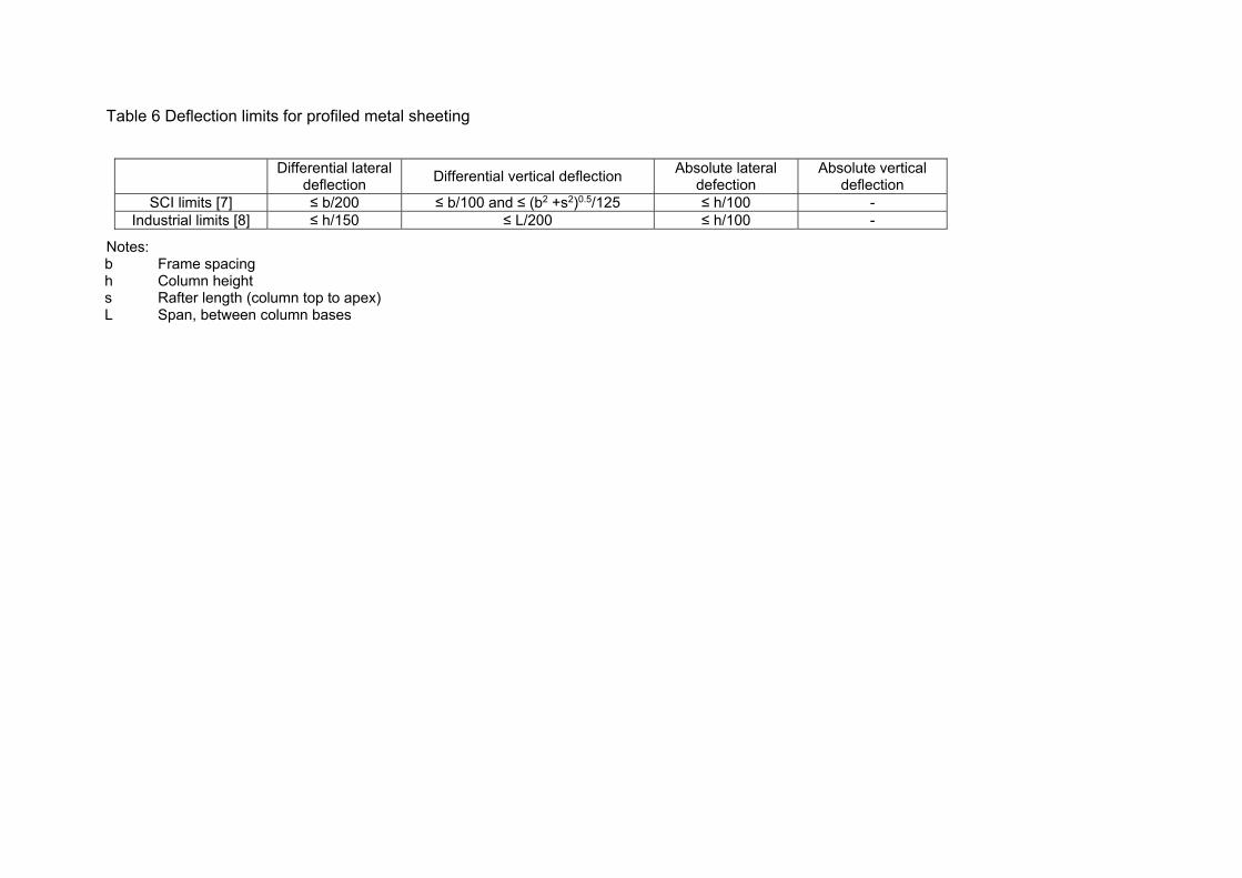
Table 6 Deflection limits for profiled metal sheeting

Differential lateral

deflection Differential vertical deflection

Absolute lateral defection

Absolute vertical deflection

SCI limits [7] ≤ b/200 ≤ b/100 and ≤ (b2 +s2)0.5/125 ≤ h/100 - Industrial limits [8] ≤ h/150 ≤ L/200 ≤ h/100 -

Notes:b Frame spacing h Column height s Rafter length (column top to apex) L Span, between column bases

Table 7 Parameters considered for frame geometry and actions

Parameters Values considered Span (m) 20, 27.5, 35, 42.5, 50 Column height (m) 4, 6, 8, 10 Apex ratio 0.5, 0.6, 0.7, 0.8 Snow load (N/m2) -200, -400, -600, -800 Wind load scalar* 0.5, 0.75, 1, 1.25, 1.5 PV loading (N/m2) -200, -400,-600, -800 Permanent loading (N/m2) -200, -400, -600, -800 Variable loading (N/m2) -600

*Varying the magnitude of the wind, using Belfast as a reference.

Table 8 Percentage influence of ULS load combination (LCs) on different frame components

Left column Left rafter Right rafter Right column Min Max Min Max Min Max Min Max

Load ID % Load ID % Load ID % Load ID % Load ID % Load ID % Load ID % Load ID % ID87 100.0 ID91 51.3 ID50 67.1 ID52 25.2 ID87 28.0 ID91 98.4 ID87 27.6 ID46 66.3 ID74 11.6 ID14 22.4 ID46 21.0 ID52 19.6 ID87 1.6 ID91 23.8 ID10 23.0

ID87 7.5 ID3 10.4 ID16 10.9 ID16 9.2 ID50 19.7 ID2 10.7 ID73 7.3 ID87 8.7 ID46 5.6 ID74 6.3 ID50 5.2 ID10 7.7 ID6 5.1 ID73 6.0 ID38 4.8 ID51 6.7 ID12 4.7 ID14 5.6 ID4 3.1 ID6 6.7 ID50 4.1 ID3 2.6 ID14, 3, 89, 48, 12, 69, 37, 71, 33, 35, 2, 36, 72

9.3 ID81 4.4 ID48 3.9 ID38, 52, 4, 69, 89, 16, 51, 37, 6, 81, 33, 71, 35, 15, 55, 19, 85

8.4 ID2 3.6 ID10 3.7 ID91, 55, 85, 19, 15, 17, 53

5.1 ID51 3.3 ID2 2.9 ID81, 3, 14, 74, 89, 73, 91, 15, 38, 71, 55, 4, 85, 19, 35, 36, 69, 72, 37, 33

9.8

Table 9 Parameters of GA configuration

GA configuration Number of design variables

Population size

Elite count

Termination criteria

Initial Normal Maximum number of genrations Stall generations limit*

C1 Rolled Frame 6 288 36 4 100 20

C2 Fabricated Frame 12 960 120 4 150 20

C3 Tapered Frame 15 1440 180 6 150 20

*The number of generation with no improvement before stopping the optimisation.

Table 10 Reliability of genetic algorithm for given population multiplier

Population multiplier

1 2 4 8 16

GA Mean weight (kg per m2)

(Standard deviation)

C1 Rolled 216.72 18.58 16.82 16.51 16.64

(240.94) (1.73) (0.40) (0.17) (0.19)

C2 Fabricated 19.88 17.82 16.32 16.35 16.34

(2.42) (1.53) (0.62) (0.59) (0.63)

C3 Tapered 16.61 15.01 14.59 14.44 14.25

(1.21) (0.70) (0.77) (0.72) (0.47)

Table 11 Reference frame optimum results

Mass kg/m2 (Standard deviation based on 8 runs)

Universal beams (C1) Fabricated beams (C2) Tapered beams (C3)

All ULS LCs ULS LCs 1-8 All ULS LCs ULS LCs 1-8 All ULS LCs ULS LCs 1-8

Apex ratio

Column height

Deflectionlimits

PV -400

No PV

PV -400

No PV PV -400

No PV

PV -400

No PV PV -400

No PV

PV -400

No PV

0.5 6 None 14.47 (0.56)

13.3 (0.33)

13.21 (0.16)

12.12 (0.35)

13.84 (0.5)

13.07 (0.51)

12.77 (0.55)

11.49 (1.06)

12.58 (0.5)

11.18 (0.51)

11.16 (0.55)

10.06 (1.06)

0.5 6 IND 14.85 (0.37)

14.26 (0.27)

14.66 (0.11)

14.22 (0.35)

14.3 (0.4)

13.81 (0.58)

14.02 (0.36)

13.72 (0.81)

13.66 (0.4)

13.49 (0.58)

13.49 (0.36)

13.12 (0.81)

0.5 6 SCI 18.69 (0.3)

18.74 (0.29)

18.71 (0.42)

18.95 (0.24)

17.39 (0.15)

17.65 (0.22)

17.51 (0.81)

17.27 (0.68)

15.75 (0.15)

16.3 (0.22)

15.75 (0.81)

16.3 (0.68)

0.8 6 None 15.15 (1)

13.45 (0.46)

14.75 (0.18)

12.25 (0.18)

15.32 (0.65)

13.79 (0.67)

14.22 (0.81)

12.62 (0.44)

13.42 (0.65)

11.71 (0.67)

12.75 (0.81)

10.61 (0.44)

0.8 6 IND 16.5 (0.27)

15.14 (0.53)

15.68 (0.3)

15.37 (0.57)

16.77 (0.44)

16.22 (0.37)

15.78 (0.11)

15.99 (0.2)

15.17 (0.44)

14.21 (0.37)

14.11 (0.11)

13.97 (0.2)

0.8 6 SCI 20.46 (0.28)

20.37 (0.8)

20.35 (0.84)

20.16 (0.93)

19.96 (0.19)

19.81 (0.34)

19.54 (0.44)

19.96 (0.66)

17.54 (0.19)

17.21 (0.34)

17.2 (0.44)

16.86 (0.66)

0.5 12 None 27.28 (1)

25.98 (0.45)

17.97 (0.28)

16.78 (0.16)

26.29 (0.81)

25.09 (1.95)

17.67 (0.76)

15.89 (0.55)

23.37 (0.81)

22.4 (1.95)

14.06 (0.76)

13.02 (0.55)

0.5 12 IND 42.17 (1.37)

42.23 (0.49)

42.25 (0.91)

43.09 (0.94)

38.46 (2.03)

38.21 (1.82)

38.96 (5.46)

38.94 (5.39)

36.75 (2.03)

36.84 (1.82)

36.75 (5.46)

36.81 (5.39)

0.5 12 SCI 75.85 (1.12)

75.83 (0.8)

75.85 (1.17)

75.76 (2.29)

61.1 (1.65)

61.5 (2.97)

62 (2.14)

62 (17.37)

60.74 (1.65)

59.78 (2.97)

58.14 (0.14)

57.8 (17.37)

0.8 12 None 28.18 (1.02)

25.84 (0.27)

19.01 (0.2)

16.5 (0.92)

27.47 (1.19)

25.88 (0.89)

19.18 (0.95)

16.38 (0.65)

24.2 (1.19)

23.45 (0.89)

16.95 (0.95)

13.85 (0.65)

0.8 12 IND 44.7 (0.85)

44.8 (0.72)

44.35 (0.86)

44.27 (0.94)

41.94 (1.16)

40.65 (5.26)

40.37 (4.45)

41.26 (2.6)

38.3 (1.16)

38.05 (5.26)

38.3 (4.45)

39.07 (2.6)

0.8 12 SCI 79.51 (1.06)

79.37 (1.45)

79.42 (2.04)

79.46 (1.28)

66.7 (1.65)

64.86 (1.83)

67 (4.17)

67 (10.05)

62.07 (1.65)

63.71 (1.83)

62.45 (4.17)

60.72 (7.05)

Table 12 Percentage increase going from symmetric to asymmetric topography

Universal beams (C1) Fabricated beams (C2) Tapered beams (C3)

All ULS LCs ULS LCs 1-8 All ULS LCs ULS LCs 1-8 All ULS LCs ULS LCs 1-8

Column height (m)

Deflection limits

PV-400 No PV PV-400 No PV PV-400 No PV PV-400 No PV PV-400 No PV PV -400 No PV

6 None 4.7% 1.1% 11.7% 1.1% 10.7% 5.5% 11.4% 9.8% 6.7% 4.7% 14.2% 5.5% 6 IND 11.1% 6.2% 7.0% 8.1% 17.3% 17.5% 12.6% 16.5% 11.1% 5.3% 4.6% 6.5% 6 SCI 9.5% 8.7% 8.8% 6.4% 14.8% 12.2% 11.6% 15.6% 11.4% 5.6% 9.2% 3.4% 12 None 3.3% -0.5% 5.8% -1.7% 4.5% -3.1% 8.5% 3.1% 3.6% 4.7% 20.6% 6.4% 12 IND 6.0% 6.1% 5.0% 2.7% 9.0% -6.0% 3.6% 6.0% 4.2% 3.3% 4.2% 6.1% 12 SCI 4.8% 4.7% 4.7% 4.9% 9.2% -5.2% 8.1% 8.1% 2.2% 6.6% 7.4% 5.1%

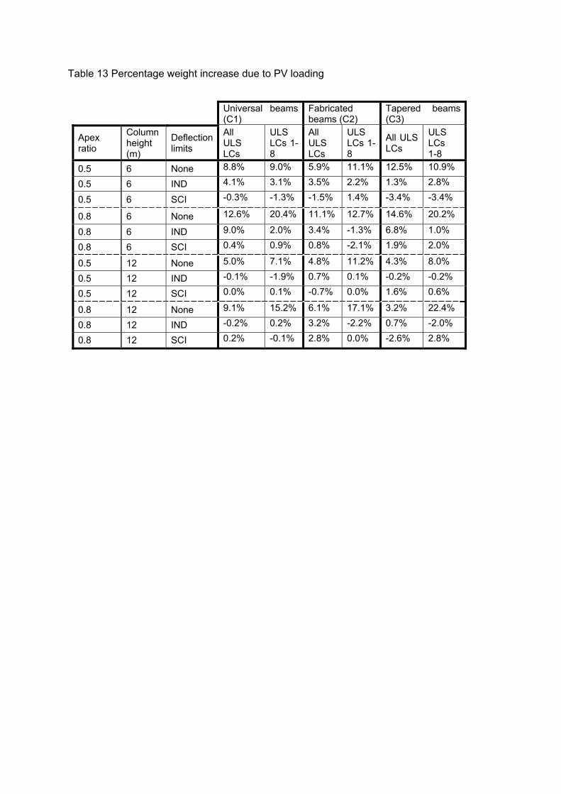
Table 13 Percentage weight increase due to PV loading

Universal beams (C1)

Fabricated beams (C2)

Tapered beams (C3)

Apex ratio

Column height (m)

Deflection limits

All ULS LCs

ULS LCs 1-8

All ULS LCs

ULS LCs 1-8

All ULS LCs

ULS LCs 1-8

0.5 6 None 8.8% 9.0% 5.9% 11.1% 12.5% 10.9%

0.5 6 IND 4.1% 3.1% 3.5% 2.2% 1.3% 2.8%

0.5 6 SCI -0.3% -1.3% -1.5% 1.4% -3.4% -3.4%

0.8 6 None 12.6% 20.4% 11.1% 12.7% 14.6% 20.2%

0.8 6 IND 9.0% 2.0% 3.4% -1.3% 6.8% 1.0%

0.8 6 SCI 0.4% 0.9% 0.8% -2.1% 1.9% 2.0%

0.5 12 None 5.0% 7.1% 4.8% 11.2% 4.3% 8.0%

0.5 12 IND -0.1% -1.9% 0.7% 0.1% -0.2% -0.2%

0.5 12 SCI 0.0% 0.1% -0.7% 0.0% 1.6% 0.6%

0.8 12 None 9.1% 15.2% 6.1% 17.1% 3.2% 22.4%

0.8 12 IND -0.2% 0.2% 3.2% -2.2% 0.7% -2.0%

0.8 12 SCI 0.2% -0.1% 2.8% 0.0% -2.6% 2.8%

Table 14 Weight increase going from ULS load combination 1-8 to all ULS load combination

Universal beams

(C1) Fabricated beams

(C2) Tapered beams

(C3)

Apex ratio

Column height (m)

Deflection limits

PV-400 No PV PV-400 No PV PV-400 No PV

0.5 6 None 9.5% 9.74% 8.38% 13.7% 12.7% 11.1%

0.5 6 IND 1.30% 0.28% 2.00% 0.66% 1.26% 2.82%

0.5 6 SCI -0.11% -1.11% -0.69% 2.20% 0.00% 0.00%

0.8 6 None 2.71% 9.80% 7.74% 9.27% 5.25% 10.3%

0.8 6 IND 5.23% -1.50% 6.27% 1.44% 7.51% 1.72%

0.8 6 SCI 0.54% 1.04% 2.15% -0.75% 1.98% 2.08%

0.5 12 None 51.8% 54.8% 48.7% 57.9% 66.2% 72.0%

0.5 12 IND -0.19% -2.00% -1.28% -1.87% 0.00% 0.08%

0.5 12 SCI 0.00% 0.09% -1.45% -0.81% 4.47% 3.43%

0.8 12 None 48.2% 56.6% 43.2% 58.0% 42.8% 69.3%

0.8 12 IND 0.79% 1.20% 3.89% -1.48% 0.00% -2.61%

0.8 12 SCI 0.11% -0.11% -0.45% -3.19% -0.61% 4.92%