Embed Size (px)
Citation preview

Comparison of techniques for measuring the water content of soil and other porous
media
Brendan Hugh George BScAgr (Hons)
Department of Agricultural Chemistry & Soil Science University of Sydney
New South Wales Australia
A thesis submitted in the fulfillment of the requirements for the degree of Master
of Science in Agriculture
MCMXCIX

Chapter 1 – Review of the literature
1
Chapter one
A review of the literature concerning the measurement of
water in porous material
1.1. MEASURING MOISTURE STATUS OF POROUS MATERIALS
There are three common ways of measuring the moisture in porous materials viz gravimetric,
potential and volumetric measurements. The preferred determination depends on how the
information required will be employed. For example, a plant biologist may prefer to discuss
moisture with respect to potential, as this is how a plant responds to moisture in the soil-plant-
air continuum. Gravimetric determination, more correctly termed wetness, is the most widely
utilised technique (across disciplines) for moisture content determination, as it is simple and
well understood. Conversely, volumetric moisture content is most commonly used in irrigated
agriculture as the reported figures can readily be converted to volumes of water required for
optimum growth. With the development of electronic instrumentation for soil moisture
determination, the volumetric basis of soil moisture measurement is now the most utilised of
the methodologies. However, the relationship between the methodologies, the soil moisture
characteristic (Section 1.1.4.2), requires explanation to allow a comparison between available
in situ technologies.
Figure 1-1 Schematic representation of soil matrix indicating relationship between air (A), soil particles
(B) and water (C).

Soil, as a porous medium, can be considered with respect to moisture status, a combination of
three components: air, solid, and water. The relationship between the three components as
shown in Figure 1-1 determines how water in soil moves, its ability to act as a solvent and its
availability to plants.
1.1.1 Wetness
The most common method for determination of moisture in soil is by removing a physical
sample from the site in question. The sample is weighed, dried in an oven at 100 °C to 110 °C
for 24 to 48 hours, and then re-weighed (Reynolds, 1970a; 1970b; Gardner, 1986). The
gravimetric moisture content, termed wetness (w), is then determined:
( )dry
drywet
mass soilmass soilmass soil −
=w (1-1)
The advantage of this system is that samples are easily acquired and the moisture content
readily determined. However, this is offset by the method being destructive in nature, thus
disallowing repeated sampling at the same location in the field. Secondly, the w (Mg Mg-1),
though a good indication of the moisture status, is not as useful to the plant scientist as
volumetric moisture and potential.
Variation in drying ovens (± 15 °C) set at 100 to 110 °C is common (Gardner, 1986). The
temperature variation influences the eventual dry state of the material. Water in the matrix is
considered (by Gardner) to be either structural (derived by components of the mineral lattice)
or adsorbed (attached to the lattice). Nutting (1943) indicated with representative thermal
drying curves the effect drying temperature exerts on the recorded wet mass to dry mass ratio.
A more appropriate temperature for drying could be between 165 °C and 175 °C (Gardner,
1986). However, this temperature range would affect the rate of organic matter oxidation. The
time of drying is insignificant after two days. Gardner (1986) reports a loss of 0.3 % moisture
in a silt loam sample weighed after drying at two days and then ten days. A sample of 50 to
100 g is sufficient for moisture determination, especially with respect to drying time and finer
textured soil (Reynolds, 1970a; Starr et al., 1995).
In the field a sound procedure for collection and storage of samples is important in reducing
error and increasing accuracy of actual determination. Reynolds (1970a) found that samples
could be appropriately stored for up to 168 hours with a one-percent loss in determined soil
moisture content before oven drying. The standard deviations of multiple moisture
determination (in the 0 – 80 mm layer of soil) can be reduced by accounting for percentage of

Chapter 1 – Review of the literature
3
stones present in the profile and excluding the soil surface vegetation thereby reducing the
effect of organic matter decomposition (Reynolds, 1970b). The number of samples required to
achieve a nominated estimate of the true mean with accepted standard error (from ± 10 to ± 2
%) at 95 % confidence varied from 1 - 7 to 125 samples respectively for two locations
(Reynolds, 1970b; 1970c). Reynolds (1970c) further suggested (his Table 3) that the
vegetation class is considered in determining the number of samples required. Reynolds
(1970a) does however note that the difference in wetness (w) in a sampling area is not only due
to the methodology of determination, but greatly influenced by the soil composition and
geography. That is, there is an effect of the inherent spatial variability.
Gravimetric sampling is utilised in many field studies where in situ volumetric moisture
content is calibrated against samples collected from close proximity to permanent or
temporarily placed sensors. For example see Burrows & Kirkham (1958); Greacen & Hignett
(1979); Hodgson & Chan (1979); Topp et al. (1982b); and Evett & Steiner (1995). Moisture
content determined by the gravimetric method is consistently referred to as the standard
technique for moisture measurement.
1.1.2 Energy - potential
The energy status of the water present in soil may be referred to in different terms. A measure
of the water content in soil (and other porous media), does not necessarily indicate how much
water is available to the plant (for transpiration), or the energy status of the water. Water will
move from areas of high energy to low energy with the energy status referred to as the water
potential (Kabat & Beekma, 1994). Hanks (1992) defines soil water potential as:
“the amount of work that a unit quantity of water in an equilibrium soil-water (or
plant-water) system is capable of doing when it moves to a pool of water in the
reference state at the same temperature”.

The potential is considered negative in unsaturated soil. Potential may be reported as energy
per unit mass (J kg-1), volume (kPa or MPa) or weight (m - water). The (soil) water potential
may be determined thus:
Ψ Ψ Ψ Ψw m s p= + + (1-2)
where:
Ψm is the matric potential, the potential that attracts (adhesion) and binds (cohesion) water to
the soil, (Yeh & Guzman-Guzman, 1995). Hanks (1992) expresses the Ψm as the vertical
distance between a point in the soil and the water level of a manometer connected to that
point;
Ψs is the solute (osmotic) potential and is related to the presence of dissolved substances in the
soil. The solute potential is normally neglected in water potential calculations except in
saline (Rawlins & Campbell, 1986) and semi-arid situations (Carrow et al., 1990), and;
Ψp is the pressure potential, defined by Hanks (1992) as the vertical distance from a point in
question to the free water surface. The pressure (submergence) potential is a measure of the
pressure exerted on a point by the overburden pressure. Pressure potential can be measured
by a piezometer and in unsaturated soil is zero and therefore neglected (Yeh & Guzmann-
Guzmann, 1995).
To obtain the overall potential the effect of gravity needs to be considered and the total
potential is determined as:
Ψ Ψ Ψt w g= + (1-3)
Noting Ψt is the total potential, and Ψg is the gravitational potential, the vertical distance from
an arbitrary reference elevation to the measurement point.
Though potential is generally the primary factor influencing movement of water through soil,
other components such as thermal and electrical gradients, discussed in detail by Rose (1968)
and Campbell (1988), can affect water movement. Corey & Klute (1985) review the
development of the “total soil water potential” concept and question the process of water
movement. The need to separate the mechanical effect (diffusion) and the chemical effect
(convection) assuring both independently have zero fluxes for measurement is highlighted.
Corey & Klute (1985) validate this position by relating the ability of the total potential concept
to drive the process of water movement to inherent membrane permeability to solute transport.
If this process is accepted then their conclusion that no single potential (as a function of the

Chapter 1 – Review of the literature
5
soil solution) will indicate the direction of net transport of the water component is reasonable.
A detailed discussion of this theory and the distillation of fundamental components of total
potential are beyond the scope of this discussion.
The soil water potential has a unique relationship with the volumetric soil water content. This
relationship, termed the soil moisture characteristic, is determined primarily by soil type and
soil aggregation and is discussed further in Section 1.1.4.2. The complexity of the relationship
between soil moisture and potential in soil complicates the ability to convert from one unit to
another especially with respect to continued in situ measurements. This complexity detracts
from the use of potential-based instrumentation for irrigation management.
1.1.3 Volumetric moisture content
Water status of soil can be determined on a volume basis, θ (m3 m-3), where θ is the volume of
the liquid phase per unit bulk volume of soil. This is the most popular method of reporting the
moisture status of soil with respect to repeated in situ measurement, especially regarding
irrigation scheduling. θ is calculated from wetness if the bulk density of the soil is known (or
estimated) as shown in Equation 1-4:
w
bwρρ
θ ×= (1-4)
Where ρb is the bulk density of the soil, (Mg m-3); ρw is the density of water (assume unity for
units of Mg m-3), and; w is wetness (Mg Mg-1) as defined in Equation 1-1.
Most in situ techniques are field calibrated to account for bulk density effects and report
moisture on a volume basis. The accuracy of the bulk density and wetness determination
dictates the accuracy of the calculated volumetric moisture content as discussed by Gardner
(1986). The determination of soil bulk density is discussed in further detail in Section 1.1.4.1.

1.1.4 Relationship of methodologies
1.1.4.1 Bulk density
To allow for a comparison between techniques, parameters such as bulk density and
relationships such as the soil moisture characteristic require consideration. The bulk density
(ρb) of the soil is an important consideration in converting w to θ as shown in Equation 1-4. In
this situation ρb is the ratio of the mass of solids to the bulk volume of the soil and is expressed
in units of mass per volume (Mg m-3). Most calculation of ρb occurs with the dry weight of
soil (Blake & Hartge, 1986). In some soil types, especially reactive clays such as those
dominated by montmorillonite and illite, a significant change between wet and dry bulk density
due to swelling and shrinkage of the sample can occur (Ross, 1985). Cullen & Everett (1995)
suggest that reporting soil moisture content is an important consideration in all ρb sampling.
As with most soil physical parameters there are several methods to estimate the in situ ρb
including: coring, clod immersion, excavation and sand replacement, and radiation methods.
The radiation methods outlined by Vomocil (1954) and Blake & Hartge (1986) will not be
discussed in detail here. The core method is based on insertion of a cylindrical metal sampler
into the soil. There are many and varied samplers with Starr et al. (1995) suggesting a
minimum diameter of 30 mm to reduce variability in measurement technique. The core is
weighed and dried (at 105 oC for 24 hours) then re-weighed. The loss of water yields w
(Equation 1-1), the ρb (Mg m3) is determined:
sampler of volume weightsoildry
=bρ (1-5)
A recent comparison of several core methods for determination of ρb indicated all methods
satisfactory “when used by a trained operator” (Dickey et al., 1993). The time taken to collect
samples with the different methods ranged from 5 minutes to 48 minutes per sample, an
important consideration for sampling budgets. Care is required in sample collection to
minimise compaction of the soil in the sampler. This is particularly relevant in extreme
conditions where wet soil may introduce error into the sampling due to viscous flow when
hammering the cylinder into the soil. Also, when the soil is very dry it may shatter, again
increasing the error associated with sampling. Careful observation during sample collection
will minimise errors arising from viscous flow and shattering (Blake & Hartge, 1986).
The sand excavation method outlined by Blake & Hartge (1986) is an ASTM (1991) method
used in surface determination of ρb, especially in loose material. Soil is excavated and

Chapter 1 – Review of the literature
7
weighed. Sand (of known mass to volume ratio) replaces the soil and ρb is determined from
this quantity.
In situ conditions occasionally inhibit the satisfactory employment of the core or sand
replacement methods. For example, if there is a significant proportion of stones in the horizon
of interest, obtaining a close fitting and undisturbed sample inside the ring can become
difficult. The wax block (or clod) method, which employs the Archimedes principle, is a
viable alternative. This method (again described in detail by Blake & Hartge, 1986) requires
an intact soil clod. The aggregate is weighed, covered in wax (paraffin) and then the
displacement is measured. Tisdall (1955) found with different soil that the wax block method
tended to overestimate ρb compared to the core method. She attributed this to the exclusion of
inter-pore spaces.
The preferred technique for determination of ρb is determined by the antecedent conditions at
sampling. The core method is the most popular and if used with consideration to potential
sampling errors is robust.
1.1.4.2 Soil moisture characteristic
Childs (1940) developed the relationship between soil water potential and soil moisture
content. This relationship is primarily determined by soil type (particularly particle size) and
influenced by physical conditions such as porosity and connectivity of pores. A schematic
example of this relationship is shown in Figure 1-2.
Figure 1-2 Soil moisture characteristic indicating effect of hysteresis. At potential A moisture content
will be between point B and C (after Payne, 1988). Changing wetting and drying cycles will
determine the resultant hysteretic curve.

The soil moisture characteristic will determine the amount of water available to the plant for
transpiration (termed available water). The available water is described variously as either the
difference between field capacity (full point) and wilting point (Hanks, 1992), or the difference
between field capacity and the refill point (Cull, 1992). The determination of field capacity is
vague because differing terminology is accepted. Generally speaking, field capacity relates to
the amount of water retained in the soil after complete saturation and drainage due to
gravitation forces. Cullen & Everett (1995) and Ahuja & Nielsen (1990) discuss the
terminology in greater detail. Wilting point relates to moisture retained in the soil with a
corresponding potential too great for plants to extract water. Thus the plants wilt and even
after the addition of water will not recover. In production agriculture the refill point is
determined by a marked decrease in the daily water use of the plant (assuming similar
meteorological conditions) and corresponds to loss of production due to moisture stress
(Briscoe, 1984). Care needs to be exercised when utilising the moisture characteristic as the
relationship is influenced by hysteresis as shown in Figure 1-2.
The relationship between the matric potential and water content, shown in Equation 1-6 (Klute
1986), relies on the determination of the two constants that not only relate to a particular soil
texture and structure, but also to the wetting history of the sample (Campbell, 1988).
Ψmba= − −θ (1-6)
Where a and b are constants for the identified soil sample. Equation 1-6 is limited in use
especially in dry soil due to (potentially) large error.
1.2. MEASURING IN SITU MOISTURE CONTENT WITH NEUTRON MODERATION
1.2.1 Introduction
The use of NMM in measurement of soil water content is widespread. The technique is
extensively used in scientific studies (e.g. Burrows & Kirkham, 1958; Greacen & Hignett,
1979; McKenzie et al., 1990; Kamgar et al., 1993) and in industry (Cull, 1992; Johnson &
Borough, 1992; Hanson & Dickey, 1993).

Chapter 1 – Review of the literature
9
1.2.2 Basis of the NMM technique
The neutron moderation technique is based on the measurement of fast moving neutrons that
are slowed (thermalised) by an elastic collision with existing hydrogen particles in the soil.
Gardner & Kirkham (1952) developed the NMM technique with others such as van Bavel et
al., (1956); Holmes (1956); and Williams et al. (1981).
The high energy, fast moving neutrons are a product of radioactive decay. Originally the
source utilised was Radium/Beryllium, however more commonly used today is
Americium/Beryllium. For example, Campbell Scientific Nuclear utilise a sealed Am241/Be
source of strength 100 mCi (=3.7×10⁻⁸ Bq). Fast neutrons (> 5 MeV) are expelled from the
decaying source following interaction between an alpha emitter (Am241) and Be. The high-
energy neutrons travel into the soil matrix where continued collisions with soil constituent
nuclei thermalise the neutrons, that is the neutron energy dissipates to a level of less than 0.25
eV. The returning thermalised neutrons collide in the detector tube (BF3) with the Boron
nuclei emitting an alpha particle that in turn creates a charge that is counted by a scalar. This
is related to the ratio of emitted fast neutrons.
The transfer of energy from the emitted fast neutron (where mass is 1.67×10⁻²¹kg) is greatest
when it collides with particles of a similar size. In the soil matrix H+ is a similar mass yielding
elastic collisions with emitted high-energy neutrons. Hydrogen (H+) is present in the soil as a
constituent of soil organic matter, soil clay minerals, and water. Water is the only form of H+
that will change from measurement to measurement. Therefore any change in the counts
recorded by the NMM is due to a change in the moisture with an increase in counts relating to
an increase in moisture content.
Gardner & Kirkham (1952) indicated (their Table 1) that hydrogen, due to its large nuclear
cross Section (probability that the fast neutron will interact with the atom), and increasing
scattering cross section (relative to other atoms present) as the neutrons lost energy, was very
efficient in slowing neutrons. Fast neutrons may be “lost” (captured) to the soil matrix when
elements such as fluorine, chlorine, potassium, iron (Lal, 1974; Carneiro & de Jong, 1985),
boron (Wilson, 1988b) and manganese are present. Other factors also influence the
relationship between emission of fast neutrons and soil water content affecting calibration and
are discussed in Section 1.2.3.
Considerable refinement of neutron meter design and production has occurred in the last forty
years with units now more portable and electronics more stable. Factors including the effect of

source and detector separation (Olgaard & Haahr, 1967; Wilson & Ritchie, 1986) and
temperature stabilisation of electronics have been incorporated in modern neutron meter
design.
1.2.3 NMM calibration
The need for calibration of the NMM in different porous materials invokes interesting
discussion. Neutron meters are commonly provided with (factory) standard calibrations for
use in common soil types. In Australia, Cull (1979) established a series of standard
calibrations and currently these calibrations are extensively used in the irrigation industry
(pers. comm., P. Cull; Irricrop Technologies International Pty Ltd, Australia). Other research
indicates support for a “universal calibration” encompassing the difference in neutron
scattering due to bulk density and texture (Chanasyk & McKenzie, 1986). In irrigated
agriculture, in many soil types, farmers who measure changes in moisture content commonly
utilise “universal calibrations” with reasonable success. Success of the “universal calibration”
in scientific studies is limited with field studies indicating that soil moisture determination by
the neutron moderation method is affected by other specific soil conditions. Greacen et al.
(1981) detailed, in field and laboratory conditions, a calibration procedure for the neutron
moisture method in Australian soil.
Consideration of bulk density (ρb, Mg m-3) is the major concern in calibrating the NMM in
field studies. Holmes (1966) discussed the influence of ρb on calibration with the change in ρb
affecting the macroscopic absorption cross section (for thermal neutrons). Olgaard & Haahr
(1968) disagreed with Holmes (1966) indicating the effect of ρb actually influenced the
transport cross sections of fast and slow neutrons. A multi-group neutron diffusion theory was
used by Wilson & Ritchie (1986) to show a linear response of the neutron moisture meter to a
change in matrix density and neutron scattering cross section. Comparing in situ determination
to re-packed soil, Carneiro & De Jong (1985) found a linear relationship yielded a suitable
calibration for their soil, a red-yellow Podzolic. However, Wilson & Ritchie (1986) differed in
their findings indicating that a non-linear response of the neutron moisture meter was evident
with respect to the thermal neutron absorption cross section and soil-water density. The error
associated with deriving the water content indicating the minimum error likely to be achieved
(dependent on chemical limitations of soil description) is ± 1.6 % to ± 3.5 % θ (Wilson,
1988b). Little consideration of these parameters occurs in many field studies regarding
calibration of NMM response to soil water content. Most calibrations undertaken encompass

Chapter 1 – Review of the literature
11
the errors associated with neutron capture, thermal neutron cross-section and neutron scattering
cross section as is evident by exclusion of these parameters in discussion. An example of this
is the discussion of Carneiro & de Jong (1985) where the authors contend that the difference in
slope estimation between two soils is probably due to differences in clay content, Fe and Ti
content or ρb of re-packed columns.
Field calibration of neutron meters is most commonly carried out with a linear equation (from
regression analysis) derived for a particular soil type and/or horizon in the form:
nba ×+=θ (1-7)
Where θ is the volumetric moisture content (m3 m-3); a is a constant (intercept); b is a constant
(slope); n is the neutron count or neutron count ratio. Greacen et al. (1981) indicated that
correct regression of count (ratio) on water content (water content as the independent variable)
reduced the possibility of introducing a bias to the calibration.
The neutron moisture calibration generally involves taking neutron readings in the extremes of
wet (field capacity) and dry soil and relating this to wetness (w). ρb is either calculated or
estimated to yield a neutron moisture content to known moisture content relationship. A
second method of calibration relates the determination of the neutron thermal adsorption and
diffusion constants as shown by Vachaud et al. (1977). This method is not widely used for
calibration of the NMM.
1.2.4 Field operation
A particular advantage of the NMM technique is the ability to obtain repeated measurements
down the soil profile as shown in Figure 1-3. In the field, aluminium (Carneiro & de Jong,
1985) or PVC (Chanasyk & McKenzie, 1986) tubes, are inserted into the soil and stoppered to
minimise water entry. Readings are taken at depths down the profile with a nominated count
time (e.g. sixteen seconds). Commonly in irrigated systems three aluminium tubes are then
averaged and moisture reported as a single reading. This aims to counter the effect of spatial
variability reducing the value of the measured moisture content data (Cull, 1979). Readings
may be taken with the neutron meter as a raw count or a count relative to a reading in a drum
of water or in the instrument shield (Greacen et al, 1981). The count ratio was utilised to
minimise potential drift in instrument readings. Improved stability of electronics and reduced
drift in counting mechanisms in the past fifteen years has diminished the importance of this
process. However, regular (as opposed to daily) calibration on a monthly or seasonal basis
should be carried out.
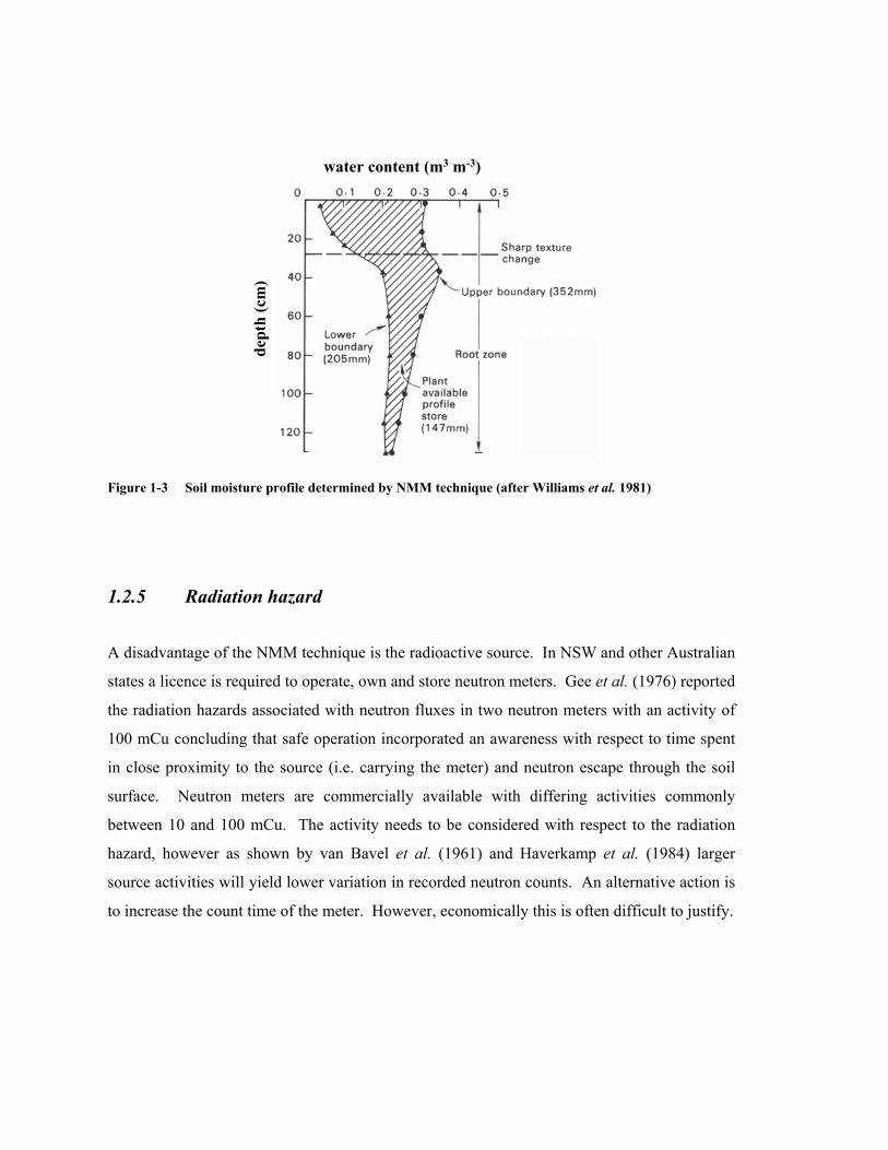
water content (m3 m-3)
dept
h (c
m)
Figure 1-3 Soil moisture profile determined by NMM technique (after Williams et al. 1981)
1.2.5 Radiation hazard
A disadvantage of the NMM technique is the radioactive source. In NSW and other Australian
states a licence is required to operate, own and store neutron meters. Gee et al. (1976) reported
the radiation hazards associated with neutron fluxes in two neutron meters with an activity of
100 mCu concluding that safe operation incorporated an awareness with respect to time spent
in close proximity to the source (i.e. carrying the meter) and neutron escape through the soil
surface. Neutron meters are commercially available with differing activities commonly
between 10 and 100 mCu. The activity needs to be considered with respect to the radiation
hazard, however as shown by van Bavel et al. (1961) and Haverkamp et al. (1984) larger
source activities will yield lower variation in recorded neutron counts. An alternative action is
to increase the count time of the meter. However, economically this is often difficult to justify.

Chapter 1 – Review of the literature
13
1.3. DIELECTRIC PROPERTIES OF SOIL
1.3.1 Introduction
The three physical components present in soil, from (Figure 1-1) are air, water and soil solid.
The electromagnetic properties of these three components at 20 °C differs from air (Kair = 1, by
definition), to solid (Ksolid ≈ 2-5), and water (Kwater = 80.18) (Weast, 1975) dominating the total
dielectric. It is this different property of the Kwater that enables the use of the dielectric
technique for moisture determination in many porous media and especially soil.
The electromagnetic properties of soil and other porous materials have been studied at length
in the past seventy years. Early work of Drake et al. (1930) and Wyman (1930) investigated
the measurement of dielectric constants in aqueous solutions. During the 1970’s advances in
electronics allowed Hipp (1974) to determine the effect of bulk density, soil moisture and
excitation frequency (30 MHz to 4 GHz) on the measured dielectric of two prepared soil
samples in an air filled coaxial line.
Soil is considered a lossy medium with dispersive properties with respect to electromagnetic
studies. The dielectric constant (K, unitless) refers to a particles’ ability to align itself with an
induced electromagnetic field and is determined by the ratio of the potential between
electrically charged plates in a non-conducting material (ε) relative to identical plates in a
vacuum (εo). The relationship (Equation 1-8) can be considered as the result of the material’s
ability to reduce the effective charge on the bodies in the medium:
Ko
= =εε
ε ’ (1-8)
Noting that K is synonymous with ε’ (permittivity); εo equals 8.85 pF m-1 (von Hippel, 1967).
K is dependant on the electrically induced polarizability of the dielectric material and the
angular frequency (ω) of the imposed field (White & Zegelin, 1995).

Soil is a conductive media with electrical losses occurring. To account for these losses
determination of the dielectric (permittivity) becomes:
K K jK* ' "= − (1-9)
Where K* is the complex dielectric (ε* permittivity); K’ is the real dielectric (ε’ permittivity)
component; K” the imaginary component (ε”); and j is an imaginary constant (√-1). The ratio
of the imaginary component (K” or ε”) to the real component (K’ or ε’) can be considered as
the phase lag between the induced electric field and the response of the dielectric:
tan"
'δ
σω ε
=
+
K
K
o
f o (1-10)
Where σo is the dc or zero frequency conductivity; and ωf the angular frequency. Often tan δ
(Equation 1-10) is assumed to be much less than one. In lossy situations, such as heavy
textured soil (bound water and surface conduction) or saline conditions; especially in relation
to larger moisture contents, this is not correct (White & Zegelin, 1995). Thus the
determination of the complex dielectric may be expressed as:
K K j K o
f o
* ' "= + +
σω ε
(1-11)
Assuming K’ >> K” then Equation 1-11 may be simplified with the measured dielectric,
termed the apparent dielectric (Ka), approximating the complex dielectric:
K Ka ≈ * (1-12)
For this relationship to hold requires tan δ << 1 (Equation 1-10).
1.3.2 The effect of frequency
The selection of the operating frequency can impact on the measured dielectric. The relaxation
time (period in which a particle can no longer orientate itself with the induced field due to
large frequency, τ) is determined by Stokes’ Law as:
τπη
=4 3r
kTm (1-13)
where η is the viscosity in relation to a liquid; T is the temperature (oK); k Boltzmann’s
constant (≈ 1.38062 × 10⁻²³); and rm is the molecular radius (White & Zegelin, 1995). For
Chapter 1 – Review of the literature
15
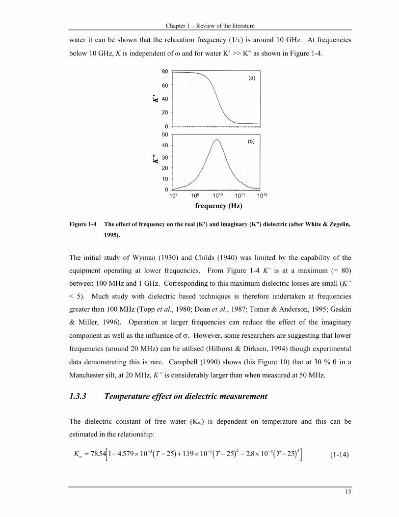
water it can be shown that the relaxation frequency (1/τ) is around 10 GHz. At frequencies
below 10 GHz, K is independent of ω and for water K’ >> K” as shown in Figure 1-4.
80
60
0
40
20
(a)
(b)50
40
0
30
20
10
frequency (Hz)108 109 101210111010
K”
K’
Figure 1-4 The effect of frequency on the real (K’) and imaginary (K”) dielectric (after White & Zegelin,
1995).
The initial study of Wyman (1930) and Childs (1940) was limited by the capability of the
equipment operating at lower frequencies. From Figure 1-4 K’ is at a maximum (= 80)
between 100 MHz and 1 GHz. Corresponding to this maximum dielectric losses are small (K”
< 5). Much study with dielectric based techniques is therefore undertaken at frequencies
greater than 100 MHz (Topp et al., 1980; Dean et al., 1987; Tomer & Anderson, 1995; Gaskin
& Miller, 1996). Operation at larger frequencies can reduce the effect of the imaginary
component as well as the influence of σ. However, some researchers are suggesting that lower
frequencies (around 20 MHz) can be utilised (Hilhorst & Dirksen, 1994) though experimental
data demonstrating this is rare. Campbell (1990) shows (his Figure 10) that at 30 % θ in a
Manchester silt, at 20 MHz, K” is considerably larger than when measured at 50 MHz.
1.3.3 Temperature effect on dielectric measurement
The dielectric constant of free water (Kw) is dependent on temperature and this can be
estimated in the relationship:
( ) ( ) ( )[ ]K T T Tw = − × − + × − − × −− − −7854 1 4 579 10 25 119 10 25 2 8 10 253 5 2 8 3. . . . (1-14)
Where T is the temperature in °K (Zegelin et al., 1992). In establishing their universal
equation, Topp et al. (1980) found temperature was not significant between 5 °C (278 °K) and
40 °C (313 °K). However in Australian conditions where near surface soil temperatures may
exceed 50 °C, correction to Kw at 25 °C (298 °K) is recommended by Zegelin et al. (1992) by
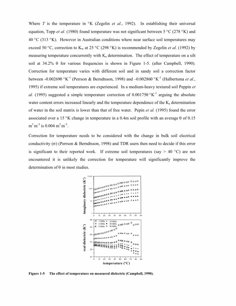
measuring temperature concurrently with Ka determination. The effect of temperature on a silt
soil at 34.2% θ for various frequencies is shown in Figure 1-5. (after Campbell, 1990).
Correction for temperature varies with different soil and in sandy soil a correction factor
between -0.00269θ °K-1 (Perrson & Berndtsson, 1998) and –0.00286θ °K-1 (Halbertsma et al.,
1995) if extreme soil temperatures are experienced. In a medium-heavy textured soil Peppin et
al. (1995) suggested a simple temperature correction of 0.00175θ °K-1 arguing the absolute
water content errors increased linearly and the temperature dependence of the Ka determination
of water in the soil matrix is lower than that of free water. Pepin et al. (1995) found the error
associated over a 15 °K change in temperature in a 0.4m soil profile with an average θ of 0.15
m3 m-3 is 0.004 m3 m-3.
Correction for temperature needs to be considered with the change in bulk soil electrical
conductivity (σ) (Perrson & Berndtsson, 1998) and TDR users then need to decide if this error
is significant to their reported work. If extreme soil temperatures (say > 40 °C) are not
encountered it is unlikely the correction for temperature will significantly improve the
determination of θ in most studies.
temperature (°C)
real
die
lect
ric
(K’)
imag
inar
y di
elec
tric
(K’)
Figure 1-5 The effect of temperature on measured dielectric (Campbell, 1990).

Chapter 1 – Review of the literature
17
1.4. TIME-DOMAIN REFLECTOMETRY (TDR)
1.4.1 Introduction
The time-domain reflectometry (TDR) technique is based on the generation of a fast rise-time
voltage pulse in either a step-wave or impulse formation. This generation and travel of the EM
wave is shown schematically in Figure 1-6 and the relationship between systems is discussed
in further detail in Section 1.4.12. Essentially, the travel time of the EM wave along probes
buried in the porous media is measured and the Ka calculated. The Ka is then related to θ either
empirically (after Topp et al., 1980) or via various physically based mixing models (e.g.
Whalley, 1993; Ferre et al., 1996). Topp et al. (1982) and Topp & Davis (1985) pioneered
field use of the technique with much development occurring in the following seventeen years
concerning hardware and software design and applications of the TDR technique. Instruments
may be adapted cable testers (e.g. Zegelin, 1992) or dedicated instruments (e.g. Skaling, 1992)
operating in a portable or stationary capacity (Baker & Allmaras, 1990; Heimovaara & Bouten,
1990; Herkelrath et al., 1991).
start point
step-pulsewaveform
impulsewaveformstart point
EM travel throughconnecting cable
end point
end point
EM wavegeneration
∆t
∆t
time (ns)
rela
tive
volta
ge
Figure 1-6 Idealised waveform generation for step pulse and impulse TDR systems

1.4.2 Measurement principle of time-domain reflectometry
A waveform in the transverse electromagnetic mode (TEM) is generated and propagated via a
shielded extension cable to an unshielded guide (called a waveguide or probe) of known length
embedded in the soil. At the end of the probe the wave is reflected due to the large impedance
and returns to the TDR instrument. This is shown schematically (after Topp et al., 1994) in
Figure 1-7. The phase velocity (vp) of a TEM in a medium is related to the apparent dielectric
and magnetic permeability (µ, H m-1) by the equation:
( )v
Kcp o=
1µ
(1-15)
Where co is the velocity of the EM wave in a vacuum (free space). The µ (4π × 10-7 H m-1 in a
vacuum; Wyseure et al., 1997) of the soil usually equals unity (Roth et al., 1992) and the loss
factor is thus neglected. The travel time of the TEM wave along the probes (of length L) is
simplified:
t Lv
=2 (1-16)
von Hippel (1967) shows the relationship between the phase velocity (v) and the dielectric
constant as:
( )v c
K
p =+ +
'
tan1 1
2
2 δ
(1-17)
Noting that tan δ (from Equation 1-10) is the loss factor. If tan δ << 1 then combining
Equation 1-16 with Equation 1-17 and rearranging simplifies to:
K c tLa =
∆2
2
(1-18)
This equation is fundamental to the TDR technique and dielectric determination in porous
media. Note that either L or 2L are used in this equation depending on the software of the TDR
system. Some systems, such as TRASE® TDR (SEC) automatically considers the travel
length ‘down and back’ along the probes (Soilmoisture Equipment Corporation, 1993). If soil
is saturated, the travel time of the EM wave along the probes is prolonged and the calculated

Chapter 1 – Review of the literature
19
Ka is large. If the soil is dry the travel time along the probes is short and the Ka is therefore
low.
Chapter 1 – Review of the literature
19
1.4.3 Electromagnetic wave reflection - determination of impedance
As the generated EM wave travels along the extension cable and into the soil guided by the
probes proportions of the wave are reflected when a change in impedance occurs. The partial
reflections reduce the energy in the EM wave and can interfere with the end-point
determination of the waveform (White & Zegelin, 1995). Initial optimism of Topp et al.
(1982a; 1982b) and Topp & Davis (1985) for multiple reflection interpretation in light textured
soil has been complicated by the effect of accounting for soil layering (Yanuka et al., 1988)
and especially attenuative media (Topp et al., 1988). The basis of multiple reflection
interpretation involves an understanding of the changing impedance on the propagating
velocity and strength of the TEM wave. The intrinsic impedance (Z) of the generated TEM is
given by the coupling of the electric and magnetic field vectors expressed as (von Hippel,
1967):
Z EH
= =µε
*
* (1-19)
For a non-conducting medium the ratio of the permeability to permittivity can be considered as
shown on the left-hand side of Equation 1-19. Lossy situations complicate the relationship
somewhat with the consideration of bulk soil electrical conductivity (σ) required (Kraus,
1984):
Z jj
=+ωµ
σ ωε (1-20)
If we persist in attempting to simplify the relationship the portion of the propagated EM wave
reflected (at the discontinuity) can be determined:
Z ZKs
a
= 0 (1-21)
Remembering the assumption in Equation 1-12, reducing µ* (= 1) in non-ferromagnetic media
and noting Zs is the impedance of a probe buried in the porous media at the end of a extension
cable with characteristic impedance, Z0 (Yanuka et al., 1988). The impedance of an extension
cable can then be calculated by:
Z Z KTDR refr
r0
11
=+−
ρρ
(1-22)
B.H. George – Measuring soil water content
20
Where ZTDR is the output impedance of the TDR instrument; Kref is the dielectric value of a
known material; and ρr is the reflection coefficient (White & Zegelin, 1995). The change of
impedance between Z0 and Zs causes the partial reflection of the EM wave and the voltage
reflection coefficient (ρr) is defined by Kraus (1984) and White & Zegelin (1995) as:
ρ rs
s
Z ZZ Z
VV
=−+
=
−0
0
1
0
1 (1-23)
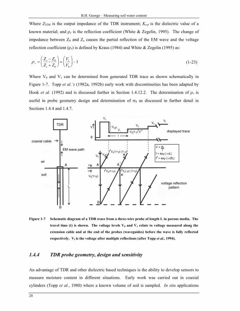
Where V0 and V1 can be determined from generated TDR trace as shown schematically in
Figure 1-7. Topp et al.’s (1982a, 1992b) early work with discontinuities has been adapted by
Hook et al. (1992) and is discussed further in Section 1.4.12.2. The determination of ρr is
useful in probe geometry design and determination of σb as discussed in further detail in
Sections 1.4.4 and 1.4.7.
air
soil
TDR
coaxial cable
EM wave path
voltage reflectionpattern
displayed trace
Figure 1-7 Schematic diagram of a TDR trace from a three-wire probe of length L in porous media. The
travel time (t) is shown. The voltage levels V0 and V1 relate to voltage measured along the
extension cable and at the end of the probes (waveguides) before the wave is fully reflected
respectively. Vf is the voltage after multiple reflections (after Topp et al., 1994).
1.4.4 TDR probe geometry, design and sensitivity
An advantage of TDR and other dielectric based techniques is the ability to develop sensors to
measure moisture content in different situations. Early work was carried out in coaxial
cylinders (Topp et al., 1980) where a known volume of soil is sampled. In situ applications
Chapter 1 – Review of the literature
21
require ready insertion of probes maintaining intimate contact with the surrounding media.
This limits the use of coaxial cells and other probes (Figure 1-8) have been developed. Recent
adaptations of probes include a hollow probe capable of simultaneous ψ measurement with θ
(Baumgartner et al., 1994); a coil probe for “point based” measurement (Nissan et al., 1998);
and a surface probe (White & Zegelin, 1995) though no detail of its performance is reported.
Zegelin et al. (1989; 1992) and Heimovaara (1993) offer a detailed discussion on probe design.
(a)
(c)
(b)
(d)
metal shield
coaxial cablecoaxial cableinsertion rodsinsertion rods
insertion rods
plastic dielectricmetal shield
shield
rod
plastic dielectricy
xz
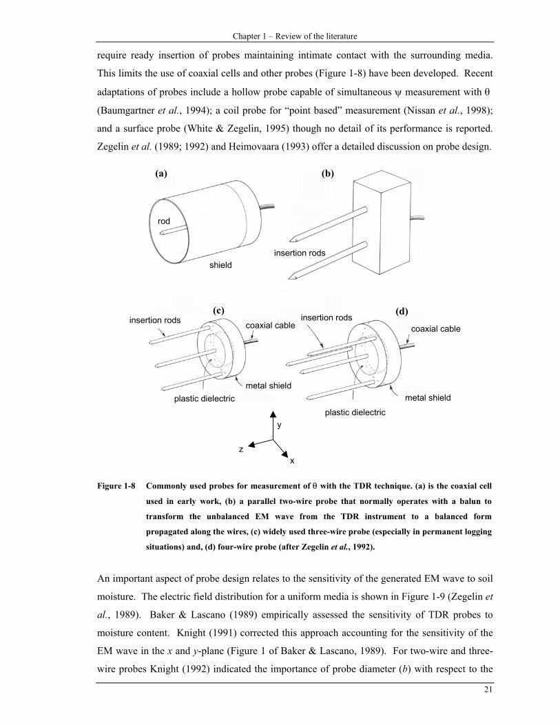
Figure 1-8 Commonly used probes for measurement of θ with the TDR technique. (a) is the coaxial cell
used in early work, (b) a parallel two-wire probe that normally operates with a balun to
transform the unbalanced EM wave from the TDR instrument to a balanced form
propagated along the wires, (c) widely used three-wire probe (especially in permanent logging
situations) and, (d) four-wire probe (after Zegelin et al., 1992).
An important aspect of probe design relates to the sensitivity of the generated EM wave to soil
moisture. The electric field distribution for a uniform media is shown in Figure 1-9 (Zegelin et
al., 1989). Baker & Lascano (1989) empirically assessed the sensitivity of TDR probes to
moisture content. Knight (1991) corrected this approach accounting for the sensitivity of the
EM wave in the x and y-plane (Figure 1 of Baker & Lascano, 1989). For two-wire and three-
wire probes Knight (1992) indicated the importance of probe diameter (b) with respect to the
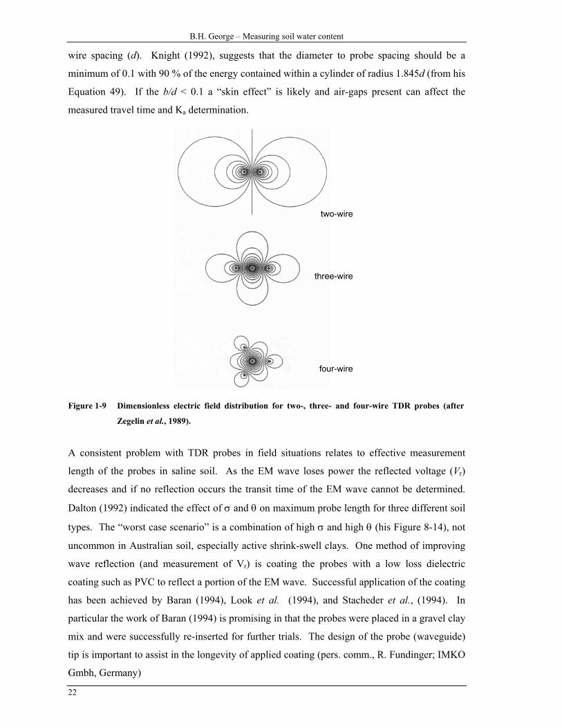
B.H. George – Measuring soil water content
22
wire spacing (d). Knight (1992), suggests that the diameter to probe spacing should be a
minimum of 0.1 with 90 % of the energy contained within a cylinder of radius 1.845d (from his
Equation 49). If the b/d < 0.1 a “skin effect” is likely and air-gaps present can affect the
measured travel time and Ka determination.
two-wire
three-wire
four-wire
Figure 1-9 Dimensionless electric field distribution for two-, three- and four-wire TDR probes (after
Zegelin et al., 1989).
A consistent problem with TDR probes in field situations relates to effective measurement
length of the probes in saline soil. As the EM wave loses power the reflected voltage (Vr)
decreases and if no reflection occurs the transit time of the EM wave cannot be determined.
Dalton (1992) indicated the effect of σ and θ on maximum probe length for three different soil
types. The “worst case scenario” is a combination of high σ and high θ (his Figure 8-14), not
uncommon in Australian soil, especially active shrink-swell clays. One method of improving
wave reflection (and measurement of Vr) is coating the probes with a low loss dielectric
coating such as PVC to reflect a portion of the EM wave. Successful application of the coating
has been achieved by Baran (1994), Look et al. (1994), and Stacheder et al., (1994). In
particular the work of Baran (1994) is promising in that the probes were placed in a gravel clay
mix and were successfully re-inserted for further trials. The design of the probe (waveguide)
tip is important to assist in the longevity of applied coating (pers. comm., R. Fundinger; IMKO
Gmbh, Germany)
Chapter 1 – Review of the literature
23
0
0.1
0.2
0.3
0.4
0.5
0.6
0.7
0.8
0.9
1
0 10 20 30 40 50 60 70 80
Measured Ka
repo
rted
thet
a
TRASE TDR
Topp et al. (1980)
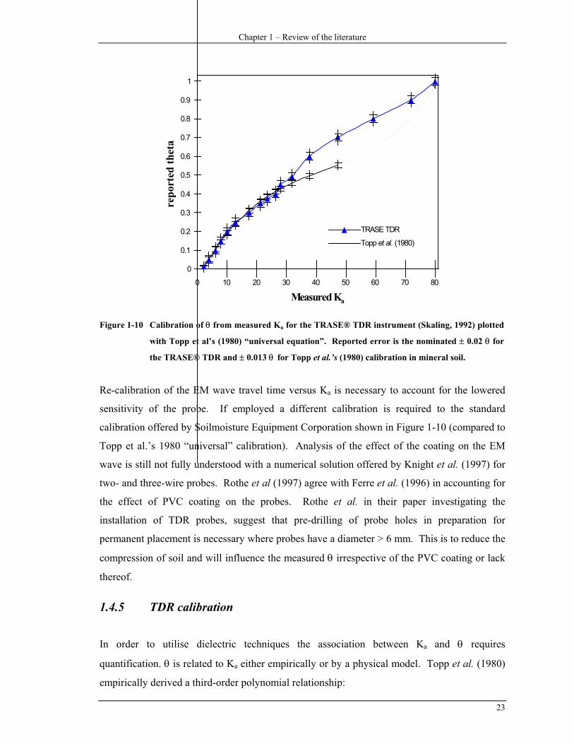
Figure 1-10 Calibration of θ from measured Ka for the TRASE® TDR instrument (Skaling, 1992) plotted
with Topp et al’s (1980) “universal equation”. Reported error is the nominated ± 0.02 θ for
the TRASE® TDR and ± 0.013 θ for Topp et al.’s (1980) calibration in mineral soil.
Re-calibration of the EM wave travel time versus Ka is necessary to account for the lowered
sensitivity of the probe. If employed a different calibration is required to the standard
calibration offered by Soilmoisture Equipment Corporation shown in Figure 1-10 (compared to
Topp et al.’s 1980 “universal” calibration). Analysis of the effect of the coating on the EM
wave is still not fully understood with a numerical solution offered by Knight et al. (1997) for
two- and three-wire probes. Rothe et al (1997) agree with Ferre et al. (1996) in accounting for
the effect of PVC coating on the probes. Rothe et al. in their paper investigating the
installation of TDR probes, suggest that pre-drilling of probe holes in preparation for
permanent placement is necessary where probes have a diameter > 6 mm. This is to reduce the
compression of soil and will influence the measured θ irrespective of the PVC coating or lack
thereof.
1.4.5 TDR calibration
In order to utilise dielectric techniques the association between Ka and θ requires
quantification. θ is related to Ka either empirically or by a physical model. Topp et al. (1980)
empirically derived a third-order polynomial relationship:

B.H. George – Measuring soil water content
24
3a
-62a
-4a
-2-2 K104.3+K105.5-K102.92+10-5.3= ××××θ (1-24)
The universal calibration predicted the θ (± 0.025 m3 m-3) from measured Ka for mineral soil
between 10 °C < T < 36 °C for the range of moisture contents 0 < θ < 0.55 m3 m-3 with a
variation in ρb from 1.14 to 1.44 Mg m-3. This equation still forms the basis of most reported θ
by the TDR technique (Topp & Davis, 1985; Zegelin et al., 1989; Zegelin et al., 1992; and
Topp et al., 1994). To account for organic soil Roth et al. (1992) developed Equation 1-25 and
Equation 1-26 for ferric soil. The ferric soil (Rhodic ferralsols, FAO) magnetic permeability
(µ) at 30 MHz was measured at 1.01 and 1.04 with 18.4 % and 18.5 % iron respectively (Roth
et al., 1992). They concluded that if errors of ± 0.015 m3 m-3 for mineral soil and ± 0.035 m3
m-3 for organic soil are acceptable then site specific calibration was unnecessary.
( )K θ θ θ θ= + + +0994 1051 8854 28922 3. . . . (organic soil, r2 = 0.996, SD = 2.52) (1-25)
( )K θ θ θ θ= − + −392 4607 374 3202 3. . (ferric soil, r2 = 0.987, SD = 1.59) (1-26)
The empirical relationship K(θ) is limited by conditions such as dry soil (θ < 0.05) where the
Ksoil dominates (Zegelin et al., 1992) and in other porous media such as grain and ore (Zegelin
& White, 1994). Further questions relating heavy soil types and the effect of bound water
(Dirksen & Dasberg, 1993), especially in Australian conditions (Bridge et al., 1996), have
focussed research towards determining a physically based relationship between measured Ka
and reported θ. Other research has identified site or soil specific problems, e.g. influence of
minerals such as iron (Robinson et al., 1994).
1.4.6 The refractive index and mixing models
More recently, a linear relationship between θ and √Ka (termed the refractive index) has been
introduced in TDR calibration studies. This term, used extensively in dielectric studies (e.g.
Fellner-Feldegg, 1969), was initially reported in soil TDR research by Herkelrath et al. (1991)
in their equation 6. The derivation of √Ka should be considered. Remembering Equation 1-15
and considering soil as a lossy medium, the ratio of the propagating velocity (co) in a vacuum
to that of the dielectric is termed the index of refraction:
Chapter 1 – Review of the literature
25
η ε µε µ
= =cv
o
p o o
* *
(1-28)
Where vp is the velocity of propagation. Remembering the complex dielectric ( **
εεoK = ) and
accounting for the magnetic equivalent:
Kmo
**
=µµ
(1-29)
The vp can be determined by:
v cK K
po
m
=* *
(1-30)
This equation is Equation 1-15 as K*m (also termed µ) equals unity in non-ferromagnetic
media. The term, √K* is reported as √Ka (from Equation 1-12) and is termed the refractive
index.
Whalley (1993), using a mixing model, derived a linear relationship between the √Ka and θ
incorporating ρb:
1)1(65.2
)1( +−+−= sb
wa KKKρ
θ (1-31)
Whalley (1993) plotted previously published data (Zegelin et al., 1989 - Bungendore sand)
with a Redhill sand yielding similar slopes and intercepts. An important consideration
however is the effect of bound water in the soil matrix due to the change in dielectric
properties. Equation 1-31 does not account for this change in dielectric properties. White et
al. (1994) questioned Whalley’s (1993) finding regarding the slope of Equation 1-31 (√K’w -1
= 8.56). They calculated the slope of Equation 1-31 in bulk water to be 7.933 < √Ka,w -1 <
7.966 and significantly different to that of Whalley (1993). Whalley (1994) argues that though
scientifically the linear calibration is empirically derived (and therefore similar to the approach
of Topp et al. (1980) and others), pragmatically the actual differences calculated by White et
al. (1994) are not important as θ determination varies by little more than 1 %. However, White
et al.’s point remains that many models offered are in fact a semi-empirical calibration.
Further, the a priori knowledge required often renders the relationship unusable in field
conditions.
B.H. George – Measuring soil water content
26
Returning to the discussion on the use of models, Ferre et al. (1996) report the K(θ)
relationship as:
bKa a +=θ (1-32)
Where a and b are constants. To use the √Ka a measurement of the parameters a and b is then
required. The relationship of travel time along the probe in soil to that of the probe in air
(T/Tair) is plotted (Hook & Livingston, 1996) yielding a slope (1/√Kw-1= 0.1256 at 20 oC) for
non clay soil, similar to that found by Herkelrath et al. (1991). The intercept is determined by
comparing the travel time along probes in air to the travel time along the same probes in oven
dry soil (Ts/Tair) where common values range from 1.4 to 1.7. The applicability of this
research to a wide range of soil types is yet to be considered, especially with respect to clay
soil and the effect of bound water.
Whalley (1993) used a simplified mixing model to derive the √Ka to θ relationship. Tinga et
al. (1973) developed a two-phase model to estimate Ka:
( )K K Ka a a b b= +φ φα α α1
(1-33)
Where φ is the volume fraction for components a and b respectively and α is a geometrical
parameter (adapted from Zegelin et al., 1992). When the field is parallel to the measurement,
α = 1, and when the field is perpendicular, α = -1. Application of a mixing model approach
(van Loon et al., 1991) in frozen and unfrozen soil yielded results similar to Topp et al.’s
(1980) empirical relationship. Dirksen & Dasberg (1993) also utilised the theoretical mixing
Maxwell-De Loor model (rewritten by Dobson et al., 1985) to quantify the relationship of Ka
and θ. This model, Whalley (1993) presented in a simplified format as:
K K K Ks s w w a aα α α αφ φ φ= + + (1-34)
Again α is a mixing parameter constant; and subscripts s, w, and a relate to solid, water and air
respectively. Roth et al. (1990), using a “composite dielectric approach”, developed a
calibration for the TDR technique with an associated error of ± 0.013 m3 m-3. Roth and his co-
workers concluded that to achieve this calibration, further parameters such as porosity (η) and
the dielectric determination of the soil matrix need to be assessed, especially in dry soil.
Dirksen & Dasberg (1993) separated the water component of the model to account for tightly
held “bound” water in the soil matrix. They preferred the Maxwell-De Loor model (their
Equation 2) to the α mixing model. As opposed to Roth et al. (1990) who used an
approximation of the geometric parameter (α = 0.46), Dirksen & Dasberg (1993) found α
Chapter 1 – Review of the literature
27
varied between -0.10 < α < 0.81 (for seven mineral soils). Zegelin et al. (1992), in controlled
conditions with the electric field perpendicular to the layering (α = -1), found the assumption
of the dielectric medium being immersed in a uniform electric field (e.g. between parallel
plates of a capacitor) to be invalid with the TDR technique utilising probes. The expectation of
the mixing model that isotropic conditions exist is not valid along the unshielded probes in
soil. This is related to the sensitivity of measurement along the probes in the soil matrix as
discussed in detail in Section 1.4.4.
A physically based calibration is preferred in determining the K(θ) relationship in soil
(Whalley, 1993). However, until now the extra parameters required (Roth et al., 1990; Bohl &
Roth, 1994; Malicki et al., 1996) have deterred most users from employing physically derived
mixing models and the use of the refractive index. White et al. (1994) though acknowledging
the benefit of such an approach, suggest that most physically derived models are in fact “semi-
empirical”. The majority of reported θ measurements by the TDR technique is determined by
the Topp et al. (1980) “universal” empirical Equation 1-24 or derivatives thereof (e.g. Skaling,
1992).
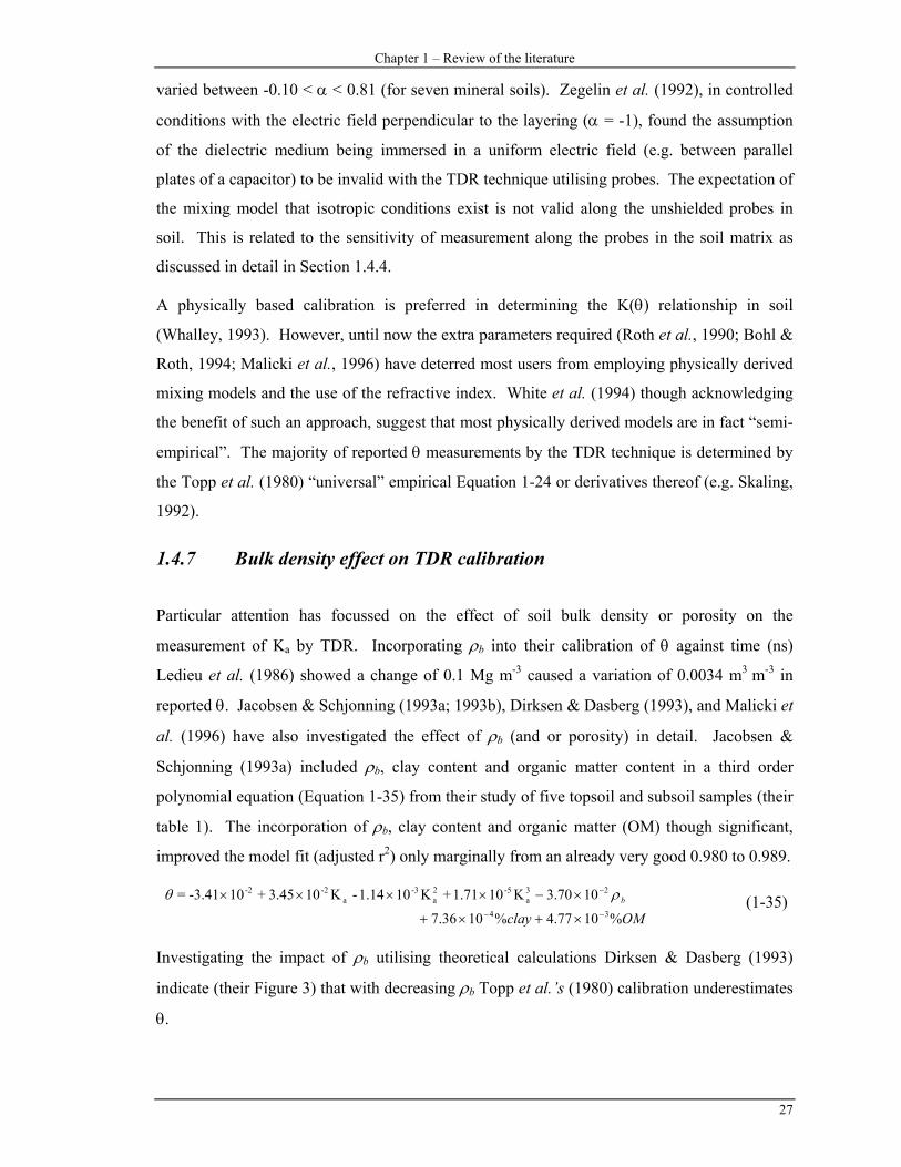
1.4.7 Bulk density effect on TDR calibration
Particular attention has focussed on the effect of soil bulk density or porosity on the
measurement of Ka by TDR. Incorporating ρb into their calibration of θ against time (ns)
Ledieu et al. (1986) showed a change of 0.1 Mg m-3 caused a variation of 0.0034 m3 m-3 in
reported θ. Jacobsen & Schjonning (1993a; 1993b), Dirksen & Dasberg (1993), and Malicki et
al. (1996) have also investigated the effect of ρb (and or porosity) in detail. Jacobsen &
Schjonning (1993a) included ρb, clay content and organic matter content in a third order
polynomial equation (Equation 1-35) from their study of five topsoil and subsoil samples (their
table 1). The incorporation of ρb, clay content and organic matter (OM) though significant,
improved the model fit (adjusted r2) only marginally from an already very good 0.980 to 0.989.
OMclayb
%1077.4%1036.7
1070.3K101.71+K101.14-K103.45+10-3.41=34
23a
-52a
-3a
-2-2
−−
−
×+×+
×−×××× ρθ (1-35)
Investigating the impact of ρb utilising theoretical calculations Dirksen & Dasberg (1993)
indicate (their Figure 3) that with decreasing ρb Topp et al.’s (1980) calibration underestimates
θ.

B.H. George – Measuring soil water content
28
To increase sensitivity in the θ(K) relationship to the change in ρb we can normalise with
respect to ρb, giving (Malicki et al., 1996):
( )b
bbb ρ
ρρθ ρ
1.18+7.170.159-0.168-0.819-K
=2
a,Ka (1-36)
In a field study conducted by Jacobsen & Schjonning (1993b) the authors found that the
inclusion of ρb did not improve their laboratory calibration equation (Equation 1-35)
concluding this was due to the small improvement offered versus the uncertainty of
measurement.
Jacobsen & Schjonning (1993a) considered that an increase in ρb yields a corresponding
increase in specific surface area leading to higher Ka. This finding concurs with those of
Dirksen & Dasberg (1993) where their theoretical calculations (their Figure 2) with the
Maxwell-De Loor model indicate that with increasing specific surface the actual θ will
increase for the same measured Ka.
transmitted EM pulse
refle
ctio
nco
effic
ient
volta
ge
zero timemark
+ 50 nstime mark
+ 100 nstime mark
time (ns)
desiredoperating range desired
operating range
pulling
ringingt1
Vth
time (ns)
Figure 1-11 Relationship for a Tektronix 1502B/C TDR instrument of the generated waveform used for
Ka determination and the associated time base waveform used to determine the actual travel
time of the propagated TEM pulse (after Hook & Livingstone, 1995).

Chapter 1 – Review of the literature
29
1.4.8 Bulk soil electrical conductivity (σ) effect on θ measurement
The bulk soil electrical conductivity (σ, S m-1) can affect the determination of θ by increasing
the K” component of the K* (Equation 1-11) from:
ωσ
+= "" pKK (1-37)
where K”p (ε”p) is the imaginary component due to polarisation losses (described in further
detail by White & Zegelin, 1995), and recalling ω is the angular frequency (rads s-1).
Thus the loss tangent (tan δ), Equation 1-10, is not much less than one as is required for
Equation 1-12 and Equation 1-18. The TDR technique is then susceptible to over estimation of
the θ as is detailed by Topp et al. (1988), Dalton (1992), White & Zegelin (1995) and Wyseure
et al. (1997). Dalton (1992) concluded when pore-water σ reaches 0.8 S m-1 over-estimation
of θ occurs. Vanclooster et al. (1993) suggest this figure could be 1.0 S m-1. Wyseure et al.
(1997) agree with the results of Vanclooster et al. (1993) suggesting that at large σ calibration
will be required. They further suggest that to avoid this situation short extension cables and
reduced length of probes will assist in end-point determination. To date there is no
comprehensive study of this limitation in Australian soil.
The real and imaginary components of K are affected by frequency as shown in Figure 1-4.
The generated EM wave may be transformed (Heimovaara, 1994a; 1994b) to yield the
operational frequencies. As discussed in detail earlier in Section 1.3.2 early studies of
dielectric properties were hampered by an inability to operate at frequencies insensitive to the
effect of soil salinity. Campbell (1990) detailed the effect of frequency on component K
between 1 to 50 MHz especially due to the ionic conductivity of the soil solution. Possible
causes of dielectric loss include charged double layers; the Maxwell-Wagner effect; bound
water; surface conductivity; and ionic conductivity, but Campbell (1990) could not (apart from
ionic conductivity) explain the change of K” with respect to frequency. Clearly the interaction
of the σ and K” in relation to dielectric losses is complex and requires further detailed
understanding. However, remember that EM loss can be minimised by generating frequencies
between 50 MHz and 10 GHz (White & Zegelin, 1995).

B.H. George – Measuring soil water content
30
Figure 1-12 Schematic diagram of effect of increasing s on waveform as determined by step-pulse TDR
system. Noting at point A the returning relative voltage (and thus reflection coefficient)
decreases as the σ increases. For θ determination the measured travel time (∆t) is important.
An advantage of the influence of σ on the TDR waveform (schematically shown in Figure 1-
12) is the ability to observe solute movement, especially through saturated soil. Much study is
being undertaken to develop a better understanding and application of this phenomenon. For
example see Topp et al. (1988); Zegelin et al. (1989); Kachanoski et al. (1992); Vanclooster et
al. (1993; 1995); Ward et al. (1994) and Kim et al. (1998). Discussion here, however, is
limited to the determination of θ by the TDR technique, and not application of the technique to
solute studies.
1.4.9 Time measurement errors
The timing mechanism employed inside the (Tektronix 1502B/C cable tester) TDR instrument
is more accurate at nominated times (12 - 42 ns, 62 - 92 ns and 112 - 142 ns) with individual
errors (47 ps) well below nominated specifications of 411 ps (Hook & Livingston, 1995).
Their experimental technique was based on the use of remotely switched diodes and a
differentiated waveform detection and is discussed further in Section 1.4.12. The effect of
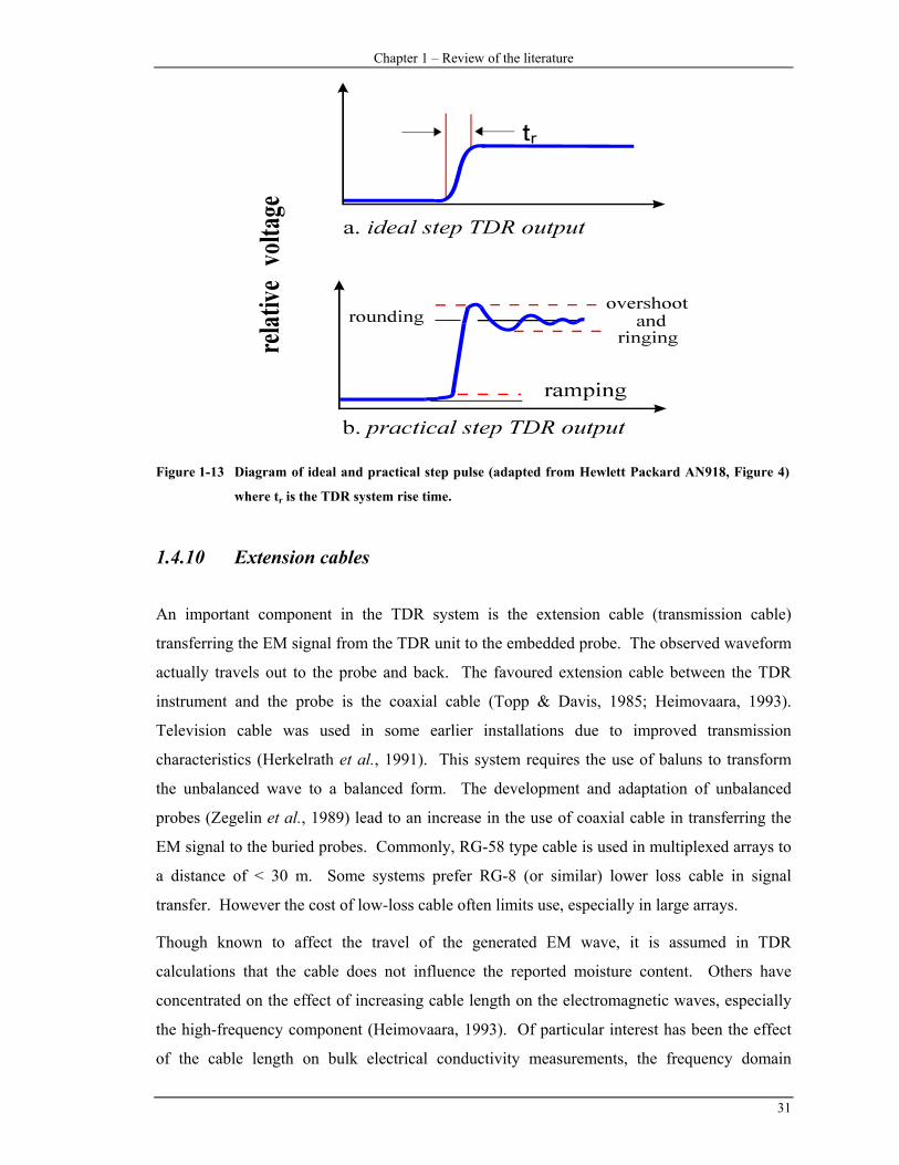
“ramping” and “ringing” on the time base marker in shown in Figure 1-10 and Figure 1-13.
This instability can lead to possible problems with waveform interpretation, especially with
long extension cable and dry sandy soil (pers. comm., J. Norris; SEC, USA). Ramping and
ringing lead to a change in generated waveform frequency with an idealised step-pulse TDR
waveform in relation to achieved waveform with current instruments shown in Figure 1-13.
Chapter 1 – Review of the literature
31
Figure 1-13 Diagram of ideal and practical step pulse (adapted from Hewlett Packard AN918, Figure 4)
where tr is the TDR system rise time.
1.4.10 Extension cables
An important component in the TDR system is the extension cable (transmission cable)
transferring the EM signal from the TDR unit to the embedded probe. The observed waveform
actually travels out to the probe and back. The favoured extension cable between the TDR
instrument and the probe is the coaxial cable (Topp & Davis, 1985; Heimovaara, 1993).
Television cable was used in some earlier installations due to improved transmission
characteristics (Herkelrath et al., 1991). This system requires the use of baluns to transform
the unbalanced wave to a balanced form. The development and adaptation of unbalanced
probes (Zegelin et al., 1989) lead to an increase in the use of coaxial cable in transferring the
EM signal to the buried probes. Commonly, RG-58 type cable is used in multiplexed arrays to
a distance of < 30 m. Some systems prefer RG-8 (or similar) lower loss cable in signal
transfer. However the cost of low-loss cable often limits use, especially in large arrays.
Though known to affect the travel of the generated EM wave, it is assumed in TDR
calculations that the cable does not influence the reported moisture content. Others have
concentrated on the effect of increasing cable length on the electromagnetic waves, especially
the high-frequency component (Heimovaara, 1993). Of particular interest has been the effect
of the cable length on bulk electrical conductivity measurements, the frequency domain
B.H. George – Measuring soil water content
32
interpretation of the TEM wave (Heimovaara, 1993; 1994; Reece, 1998). Heimovaara (1993)
found a change in the start-point determination with increasing cable length. This increased
the error of the reported q and Heimovaara suggested that minimum probe lengths (0.05 m to
0.2 m) be used with associated maximum cable lengths (≈ 3.2 m to ≈ 24.1 m respectively).
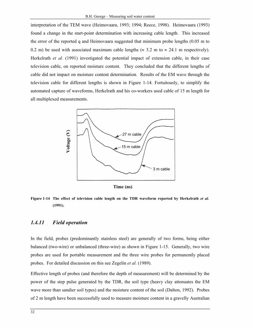
Herkelrath et al. (1991) investigated the potential impact of extension cable, in their case
television cable, on reported moisture content. They concluded that the different lengths of
cable did not impact on moisture content determination. Results of the EM wave through the
television cable for different lengths is shown in Figure 1-14. Fortuitously, to simplify the
automated capture of waveforms, Herkelrath and his co-workers used cable of 15 m length for
all multiplexed measurements.
Time (ns)
Vol
tage
(V)
3 m cable
15 m cable
27 m cable
Figure 1-14 The effect of television cable length on the TDR waveform reported by Herkelrath et al.
(1991).
1.4.11 Field operation
In the field, probes (predominantly stainless steel) are generally of two forms, being either
balanced (two-wire) or unbalanced (three-wire) as shown in Figure 1-15. Generally, two wire
probes are used for portable measurement and the three wire probes for permanently placed
probes. For detailed discussion on this see Zegelin et al. (1989).
Effective length of probes (and therefore the depth of measurement) will be determined by the
power of the step pulse generated by the TDR, the soil type (heavy clay attenuates the EM
wave more than sandier soil types) and the moisture content of the soil (Dalton, 1992). Probes
of 2 m length have been successfully used to measure moisture content in a gravelly Australian

Chapter 1 – Review of the literature
33
soil (Zegelin et al., 1992). However, in wet heavy clay soil, probe (waveguide) length has
sometimes been reduced to as little as 200 mm. This current problem is being rectified by
increasing the power and stability of the EM wave and by coating probes with a thin cover of a
low dielectric material (pers. comm., J. Norris; SEC, USA). The aim is to ensure that a
percentage of the wave will travel the length of the probes and be reflected allowing
determination of ∆t.
unbalanced balanced
unbalanced
coaxial cablestainless steelwaveguidesbalun
Figure 1-15 Schematic diagram illustrating the connection of the coaxial cable (unbalanced signal) to the
stainless steel probes through a balun for the two-wire system (balanced), and direct to the
probes in the three-wire system (unbalanced).
1.4.12 Current situation with TDR instrument development
There are several different TDR systems measuring moisture and solute transport in porous
media. The development of TDR instruments can be generalised into the two categories:
(i) step-pulse TDR systems being either, (a) Tektronix (1502 B/C) cable tester based TDR
configurations, or (b) dedicated TDR systems.
(ii) impulse TDR systems
1.4.12.1 Step-pulse TDR systems based on Tektronix cable testers
In the past twenty years the majority of TDR systems have been developed for use with the
Tektronix 1502 (Beaverton, Oregon, USA) series cable testers. These cable testers are not

B.H. George – Measuring soil water content
34
developed specifically for soil moisture determination and usually custom software programs
are written to assist in end-point determination, especially in automated situations. A tunnel
diode circuit generates a fast rising step voltage and this is then propagated via extension cable
to the probe. In its most primitive form a ruler is used to measure the ‘apparent length’ of the
wave from the Tektronix screen and then calculations are undertaken to derive the moisture
content.
Campbell Scientific TDR system
This TDR system consists of a Tektronix 1502B/C cable tester linked to a logger and
multiplexed through a series of switches and extension cables to probe in the field as shown
schematically in Figure 1-16. The cable tester is interfaced to a datalogger with the EM wave
propagated via RG58 or RG8 coaxial cable through three switching levels to 300 mm long
twin wire probes (Anonymous, 1991). Moisture content is calculated from Topp et al.’s
(1980) or Ledieu et al.’s (1986) equations. The Campbell Scientific systems are also widely
used in the engineering field (e.g. Janoo et al., 1994).
Level 1multiplexer
Level 3multiplexers
Level 2multiplexers
TDR(1502)
logger
Up to 8 multiplexersor soil probes
TDR coaxial cablecommunication cable
TDR probe
Figure 1-16 Schematic diagram of the Campbell Scientific TDR system designed for field or laboratory
studies with multiple probes (PB30) (after Campbell Scientific, 1995).
Vadose Zone Equipment
As opposed to Campbell Scientific this system operates with a laptop computer for control and
storage of information from the cable tester. The system configuration is similar to Campbell
Scientific. The system was developed from work undertaken by Evett (1994).
Other available systems

Chapter 1 – Review of the literature
35
Many scientists throughout the world have adapted TDR systems to achieve specific functions
such as irrigation scheduling or automated readings. There have been TDR systems developed
by CSIRO Environmental Mechanics (Canberra, Australia) and others (e.g. Heimovaara & de
Water, 1993). Availability of the systems is often limited to the country of origin or specific
research applications. The TDR system developed by CSIRO, Pyelab (Zegelin, 1992), is now
commercially offered through Campbell Scientific.
Figure 1-17 Schematic diagram of the TRASE® TDR system developed by Soilmoisture Equipment
Corporation (SEC technical drawing).
1.4.12.2 Dedicated step pulse TDR instruments
TRASE® TDR
Skaling (1992) details the development of the Soilmoisture Equipment Corporation TDR, the
TRASE® (Time Reflectometry Analysis of Signal Energy). This dedicated TDR instrument
differs from Tektronix based systems in architecture design (modular construction) and EM
wave generation. The TRASE® TDR system, shown schematically in Figure 1-17, uses a step
recovery diode system to generate the step pulse EM wave. Skaling (1992) reports that this
system allows greater energy in the EM wave and this increases potential extension cable
length and assists in measurement determination in attenuative materials. Data is unavailable
to support this claim. Another feature of the TRASE® TDR system is the digitising capability
with respect to the “measurement window”. The TRASE® TDR system, operating with a
B.H. George – Measuring soil water content
36
nominated measurement window, will record 1000 (or 1200 in later machines) voltage points
with time. This varies from Tektronix units that operate with 256 points. The greater number
of measurement points assists with the on-board automatic tangent fitting regimes (pers.
comm. H. Fancher; SEC, USA). The TRASE® TDR system is capable of multiplexing up to
256 probes through a double level-switching array.
TRIME TDR system
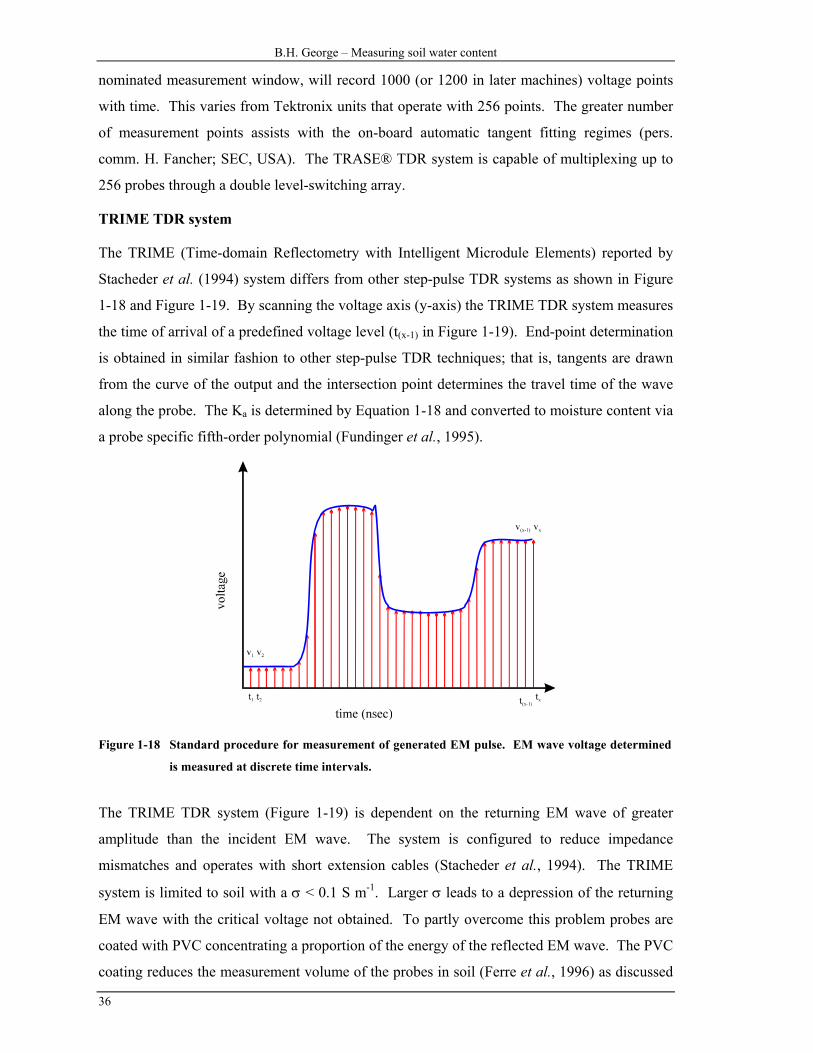
The TRIME (Time-domain Reflectometry with Intelligent Microdule Elements) reported by
Stacheder et al. (1994) system differs from other step-pulse TDR systems as shown in Figure
1-18 and Figure 1-19. By scanning the voltage axis (y-axis) the TRIME TDR system measures
the time of arrival of a predefined voltage level (t(x-1) in Figure 1-19). End-point determination
is obtained in similar fashion to other step-pulse TDR techniques; that is, tangents are drawn
from the curve of the output and the intersection point determines the travel time of the wave
along the probe. The Ka is determined by Equation 1-18 and converted to moisture content via
a probe specific fifth-order polynomial (Fundinger et al., 1995).
Figure 1-18 Standard procedure for measurement of generated EM pulse. EM wave voltage determined
is measured at discrete time intervals.
The TRIME TDR system (Figure 1-19) is dependent on the returning EM wave of greater
amplitude than the incident EM wave. The system is configured to reduce impedance
mismatches and operates with short extension cables (Stacheder et al., 1994). The TRIME
system is limited to soil with a σ < 0.1 S m-1. Larger σ leads to a depression of the returning
EM wave with the critical voltage not obtained. To partly overcome this problem probes are
coated with PVC concentrating a proportion of the energy of the reflected EM wave. The PVC
coating reduces the measurement volume of the probes in soil (Ferre et al., 1996) as discussed

Chapter 1 – Review of the literature
37
in Section 1.4.4. The ability of the TRIME system for simultaneous measurement of σ as well
as θ will be complicated by the PVC coating of the probes. The coating reduces the proportion
of propagation of low frequencies (< 300 MHz) and dc voltage of the EM wave. This will
reduce the susceptibility of the wave to attenuation that is necessary in determining the σ.
However, as shown by Stacheder et al. (1994), a relationship does exist between σ and the
amplitude (specific to the TRIME TDR) of the reflected wave (dimensionless).
Figure 1-19 TRIME method of measuring the EM wave as it travels from the TDR along the coaxial cable
and into the soil via probes (after Stacheder et al., 1994).
Moisture Point TDR
Based on the work of Hook et al. (1992, 1995), this system operates with a fast rise step pulse
EM wave. The distinguishing feature of the Moisture Point (MP) TDR system is the use of
diodes along segmented probes. This improves the signal to noise ratio. Several positive
aspects of this approach include:
• use of longer extension cable (to at least 100 m);
• improved end-point reflection in saline and heavy (clay) soil types;
• simplification of component TDR electronics;
• discrete measurement down the soil profile in one location.
The instrument can read a profile (standard configuration of five segments) in less than 90
seconds with an “absolute” accuracy of ± 2.5 %, and has a universal calibration curve with a
resolution of 1.0 % (Anonymous, 1994). Dasberg et al. (1995) calibrated the MP TDR system
successfully in the laboratory with a (Bungendore) sand. Calibration in the field indicated
greater variability and this was attributed to a small measurement volume (diameter < 10 mm)
B.H. George – Measuring soil water content
38
and inherent soil moisture variability. Another conclusion included the possibility of
preferential flow of water along the inserted probe leading to preferential water flow during
irrigation and elevated θ determination compared to other techniques such as NMM (Dasberg
et al., 1995). More recently Frueh & Hopmans (1997) successfully calibrated the segmented
probe in field and laboratory conditions for a gravelly soil. They noted that re-installation was
required for successful in situ calibration. The probes were inserted into an oversized hole and
back filled. This indicates potential problems as again the small sphere of influence can lead to
siting difficulty in situ for representative θ measurements. A detailed study of the use of MP
TDR systems in heavy soil is yet to be undertaken.
Impulse TDR systems
Malicki & Skierucha (1989), Malicki (1990) and Malicki et al. (1992) pioneered work with
impulse based TDR systems in measuring θ in porous media. Figure 1-6 schematically
indicates the relationship between an EM wave generated with an impulse-based TDR
instrument as opposed to a step-pulse generated EM wave. The EM waveform resembles the
function sin2t where 0 < t < 300 ns (Malicki, 1990). Ka is determined from measurement of the
travel time of the EM wave along the probes embedded in the porous media, as occurs with
step-pulse based TDR systems. From Figure 1-6 the impulse TDR system operates by the
introduction of a fast (< 200 psec) spike (needle) which then travels along the extension cable
and down the probes in the soil. When the EM wave reaches the end of the probes the high
impedance causes a second characteristic (though of smaller magnitude) peak. The travel time
is measured as the distance between the peaks and moisture content is then determined in a
similar fashion to step-pulse TDR calculations (Malicki & Skierucha, 1989; Malicki et al.,
1992). Malicki (1990) using an empirical approach related the measured EM wave velocity to
θ:
( )36242 1063.21081025.929.2exp vvv −−− ×−×+×−=θ (1-38)
where v is the velocity of the propagated EM wave in soil. Determination of the σ is similar to
that of step-pulse TDR systems (Malicki et al., 1994; pers. comm., M. Malicki; Polish
Academy of Sciences, Poland). Several practical questions remain about the use of impulse
TDR for moisture measurement. The problem, as with step pulse TDR systems, lies with the
tolerance of attenuation before the signal is not detectable. The impulse TDR system has not
been widely used in Australian conditions to date.
1.4.13 TDR Summary

Chapter 1 – Review of the literature
39
A summary of the various TDR systems and configurations is given in Table 1. The TDR
technique in general is developing rapidly research is increasing in developing further
applications of TDR such as surface measurements (Selker et al., 1993; White & Zegelin,
1995), profile measurements (Hook et al., 1992), long range multiplexing of probes, combined
soil water content and potential (Baumgartner et al., 1994) and solute transport determination
(e.g. Kachanoski et al., 1994).
1.5. FREQUENCY-DOMAIN (CAPACITANCE) TECHNIQUE
1.5.3 Introduction
The frequency-domain technique is similar to that of TDR in that the apparent dielectric (Ka)
relationship to moisture content (θ) is exploited. Wyman (1930) identified the relationship
between capacitance and soil moisture in the late 1920’s. However, the use of capacitance
based techniques was not possible due to the inability to select oscillating frequencies not
influenced by the bulk soil electrical conductivity (σ). Malicki (1983), following the work of
Thomas (1966), developed a working in situ capacitance based sensor. Widespread use of
frequency-domain (FD) sensors followed development of a down-hole portable instrument
(Dean et al., 1987). In a second paper evaluating the instrument, Bell et al. (1987) produced an
in situ “universal” calibration. Other FD sensors utilise short probes in a similar design to the
TDR technique (Robinson & Dean, 1993; Hilhorst & Dirksen, 1994).
Capacitance (C), measured in Farads (F), is defined as the amount of charge (Q) required to
increase the voltage (V) by one volt between two plates separated by a known distance
containing an insulating material:
C QV
= (1-39)
A high frequency transistor oscillator (generally ≈ 150 MHz) operates with the soil (dielectric)
forming part of an ideal capacitor as shown in Equation 1-40:
C K AS
o=ε (1-40)
Where K is related to C via the interaction of the total electrode area (A) and spacing of the
electrodes (S), remembering that (εo), the permittivity of free space is constant (White &
Zegelin, 1995).

TDR instrument
EM generation Source Use Multiplexing Probe configuration
Reference information
Campbell Scientific
Tektronix based, step pulse
Campbell Scientific Inc., Logan UT, USA
stationary 30m extension cable limit, 2nd and 3rd level switches
balanced systems
Baker & Allmaras (1990)
Easy Test Impulse TDR Easy Test Ltd, Lublin, Poland stationary or portable 2nd level switches, 36 channels
balanced, 50 mm probes
Malicki (1990)
Heimovaara Tektronix based, step pulse
University of Amsterdam, Amsterdam, The Netherlands
stationary 2nd level switches, 144 channels
balanced Heimovaara & de Water (1993)
Moisture point TDR
dedicated step pulse, diodes utilised
Environmental Sensors Inc, Victoria B.C., Canada
segmented probe, portable and stationary
limited (profile sensors, say four probes), 100m coax
balanced, segmented profile probe
Hook et al. (1992)
Pyelab Tektronix based, step pulse
Environmental Mechanics Laboratory, Canberra ACT, Australia
stationary 30m coax limit mainly unbalanced
Zegelin (1992)
TRASE dedicated step pulse, time digitisation
Soilmoisture Equipment Corporation, Santa Barbara CA, USA
portable and stationary 30m coax limitation, 256 channels
balanced and unbalanced
Skaling (1992)
TRIME dedicated step pulse, voltage threshold
IMKO Micromodultechnik, Ettlingen, Germany
portable or stationary 1) dumb sensor 3.6m limit (six sensors per module); 2) 2+ km smart sensor
no balun un-balanced, coated probes only
Stacheder et al. (1994)
Vadose Zone Equipment
Tektronix based, step pulse
Vadose Zone Equipment Company, Amarillo TX, USA
stationary and portable 30m coax limit, 2nd and 3rd level switches
balanced and unbalanced
Evett (1994)
Chapter 1 – Review of the literature
41
Ideally, the soil is situated between two plates (electrodes) forming a capacitor, however in a
field situation the design of the capacitance probe is not ideal with either two annular rings
(electrodes) placed within a plastic access tube in the soil, or a single electrode inserted into
the soil. The measured area is now removed from between the electrodes to outside the access
tube as shown in Figure 1-20. However, sensitivity to change in soil moisture is reduced
(Nadler & Lapid, 1996). The measurement area is considered a “fringe field” (Thomas, 1966)
as the main influence on the oscillating wave is the uniform interior of the access tube. As the
soil dielectric inside the access tube should not change, the soil water will influence the
measured capacitance. Thus in a field situation the measured C is determined as:
C gK= (1-41)
Where C is related to K via a geometrical constant (g) measured in Farads (F), (Whalley et al.,
1992). g depends upon electrode spacing, area and orientation of the electrodes in the soil and
εo (White & Zegelin, 1995). The relationship between C and frequency (F, measured in Hz) is
dependent on the operating design of the capacitance probe. For a down-hole sensor, Whalley
et al. (1992), give the relationship as:
FL C C Cb c
= + +
12
1 1 1π
(1-42)
Where L is the inductance of the oscillator; C is the measured capacitance of the sensor
elements; Cb is the base capacitance; and Cc the collector capacitance of the oscillator circuit.
Equation 1-42 may be simplified by combining the soil component capacitance and other
constants to form:
FLC
=1
2π (1-43)
This assumption is valid for FD measurement in soil if constituent parameters do not change
with time. To account for the sensor design a normalised frequency is determined (Didcot,
1992; Paltineanu & Starr, 1997):
( )( )
FF FF Fu
a s
a w
=−−
(1-44)
Where Fu is the normalised universal frequency; Fa is the frequency measured in air (inside a
PVC tube); and Fs is the measured frequency in soil (again inside a PVC tube). This process is

B.H. George – Measuring soil water content
42
used with portable (Dean et al., 1987) and stationary (Starr & Paltineanu, 1998) down-hole FD
sensors.
electrode
electrode
oscillator
PVC accesstube
fringingfield
fringingfield
Figure 1-20 Schematic diagram of capacitance probe in a PVC access tube placed vertically in the soil
(after Whalley et al., 1992).
1.5.2 FD calibration
Thomas (1966) indicated a two-step process of calibration with a linear relationship at small
values (θ < 0.10 m3 m-3), and a semi-logarithmic relationship for values 4.5 m3 m-3 < θ < 45 m3
m-3 of the form:
9.20log7.37 −∆= Cθ (1-45)
where ∆C is the measured “fringe” capacitance change to that measured in air. The form of
calibration estimation varies with log, exponential and linear calibrations employed. In a
sandy soil Mead et al. (1994) were satisfied with the latter. Utilizing a different probe system
Mead et al. (1995) again preferred a linear relationship to a (factory based) exponential based
calibration. If higher water contents are not encountered justification of a linear relationship is
acceptable (Ould Mohamed et al., 1995). Other authors including Bell et al. (1987) and
Chapter 1 – Review of the literature
43
Paltineanu & Starr (1997) still favour non-linear relationships. Kholsa & Persaud (1997)
indicate (their Figure 4) that at larger moisture contents their FD instrument lost sensitivity
with a corresponding increase in reported standard error. This is due to the calibration form
commonly used with θ exponentially related to the frequency shift. In a field calibration in a
loamy sandy soil an upper limit of 0.40 m3 m-3 for reliable results is recommended (Ould
Mohamed et al., 1995).
In a laboratory calibration of a FD sensor operating at lower frequency (see Hilhorst & Dirksen
(1994) for description) Perdok et al. (1996) found the technique sensitive to changes in ρb and
soil type. Their calibration estimated permittivity with a power relationship dependent on the
ρb. Calibration, especially with the FD technique is dependent on the sensor configuration and
operating frequency.
1.5.3 FD precision
Dean et al. (1987) and others claim that the FD technique offers an improved precision in
determination of θ compared to other in situ techniques, especially NMM. The theory
underlying the frequency shift and relationship to θ supports this claim. Field studies have
indicated however, that the FD technique is susceptible to noise (i.e. error) in determination of
θ. In a fine-loamy mixed thermic Aridic Paleustalf, Evett & Steiner (1995) estimated the root
mean square error (RMSE) of θ determination to be three times that of NMM measurement.
This lead Evett & Steiner (1995) to question the applicability of the FD technique for soil
water content measurement in heterogeneous soil. Ould Mohamed et al. (1997), using a FD
probe (in a fine loamy, mixed, mesic, Typic Eutrochrept) to account for similar textures,
considerably reduced the average 95 % confidence interval to 0.014 - 0.019 m3 m-3. This was
approximately ten times smaller than errors found by Evett & Steiner (1995). Ould Mohamed
et al. (1997) found the FD technique to be more accurate in determination of θ compared to
NMM. Notably, the calibration techniques for the two methods differed, not accounting for
the effective NMM measurement area. This issue requires further investigation, especially
concerning the different FD systems available.
B.H. George – Measuring soil water content
44
1.5.4 Influence of air-gaps on measured dielectric
The largest probable source of error in θ determination with the FD technique is related to air-
gap occurrence near access tubes that are introduced during installation (Evett & Steiner, 1995;
Bell et al., 1987). This could be a particular problem with installation of tubes at drier sites
(Evett & Steiner, 1995) or in swelling soils. This corresponds with Tomer & Anderson’s
(1995) comparison between a FD probe and NMM where the capacitance probe measurement
varied near the soil surface. Ould Mohamed et al. (1997) conclude in their discussion
regarding the error analysis of θ that the difference between FD and NMM θ determination
decreases with an increase in soil θ, especially at shallow (< 250 mm) depth. This could be
accounted for by the escape of neutrons matched by an increase in air-gaps along installed
PVC tubes. Air-gaps present in close proximity to the access tube are accentuated by the
weighting function of sphere-of-influence (Bell et al., 1987).
Commercially, there are several FD systems available for moisture determination as shown in
Table 1-2. The main advantage of the FD technology is the apparent low cost of the
components and the ease of long distance transfer (either through cables or cellular phone) of
the measurement signal.
1.5.5 Field application of FD technique
Measurement with the FD technique is undertaken by either lowering a sensor into the access
tube (Bell et al., 1987; Tomer & Anderson, 1995); placing an array of sensors into the access
tubes and logging the output frequency (Buss, 1994; Paltineanu & Starr, 1997); or by insertion
of the instrument directly into the soil (Robinson & Dean, 1993; Hilhorst & Dirksen, 1994).
Field studies by Robinson & Dean (1993), Starr & Paltineanu (1997) and Wu (1998) indicate
that the FD technique is suitable for in situ studies with considerations such as careful tube
installation. Tube installation and contact between probe and the soil has been identified as the
major constraint in FD implementation in field studies (Malicki, 1983; Bell et al., 1987; Evett
& Steiner, 1995 and Tomer & Anderson, 1995).
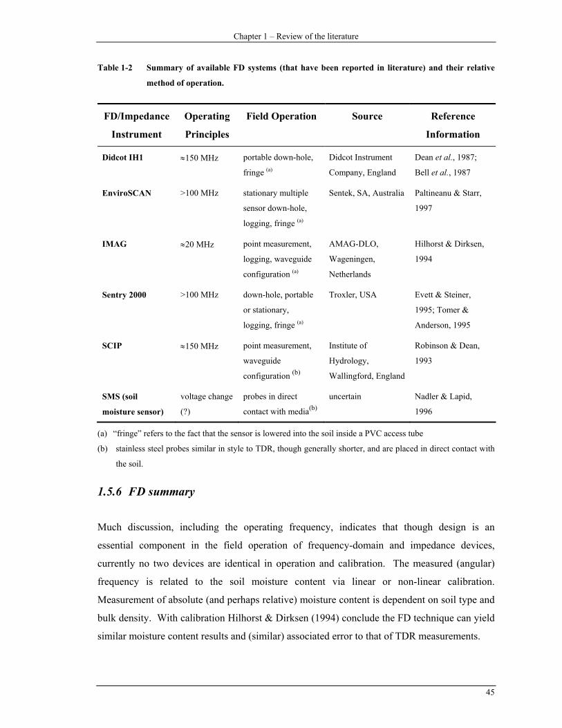
Chapter 1 – Review of the literature
45
Table 1-2 Summary of available FD systems (that have been reported in literature) and their relative
method of operation.
FD/Impedance
Instrument
Operating
Principles
Field Operation Source Reference
Information
Didcot IH1 ≈150 MHz portable down-hole,
fringe (a)
Didcot Instrument
Company, England
Dean et al., 1987;
Bell et al., 1987
EnviroSCAN >100 MHz stationary multiple
sensor down-hole,
logging, fringe (a)
Sentek, SA, Australia Paltineanu & Starr,
1997
IMAG ≈20 MHz point measurement,
logging, waveguide
configuration (a)
AMAG-DLO,
Wageningen,
Netherlands
Hilhorst & Dirksen,
1994
Sentry 2000 >100 MHz down-hole, portable
or stationary,
logging, fringe (a)
Troxler, USA Evett & Steiner,
1995; Tomer &
Anderson, 1995
SCIP ≈150 MHz point measurement,
waveguide
configuration (b)
Institute of
Hydrology,
Wallingford, England
Robinson & Dean,
1993
SMS (soil
moisture sensor)
voltage change
(?)
probes in direct
contact with media(b)
uncertain Nadler & Lapid,
1996
(a) “fringe” refers to the fact that the sensor is lowered into the soil inside a PVC access tube
(b) stainless steel probes similar in style to TDR, though generally shorter, and are placed in direct contact with
the soil.
1.5.6 FD summary
Much discussion, including the operating frequency, indicates that though design is an
essential component in the field operation of frequency-domain and impedance devices,
currently no two devices are identical in operation and calibration. The measured (angular)
frequency is related to the soil moisture content via linear or non-linear calibration.
Measurement of absolute (and perhaps relative) moisture content is dependent on soil type and
bulk density. With calibration Hilhorst & Dirksen (1994) conclude the FD technique can yield
similar moisture content results and (similar) associated error to that of TDR measurements.

B.H. George – Measuring soil water content
46
The potential for capacitance based soil moisture determination is good (Whalley et al., 1992).
However, development is required to determine the actual measurement area of the probe and
its spatial sensitivity to change in moisture content. Further, the calibration of the technique in
situ needs to more fully understood to allow universal use and the effect of electrical
conductivity, temperature and acid soil on measured frequency has not been fully studied (pers.
comm., T.J. Dean; Institute of Hydrology, England). The most pressing concern regarding the
acceptance of FD is the installation process and maintaining contact with the immediate
surrounding soil.
1.6. OTHER DIELECTRIC-BASED DEVICES
The recent development of electronics has encouraged researchers to adapt the basic design of
frequency-domain techniques in developing sensors such as the “ThetaProbe” (Gaskin &
Miller, 1996) and Campbell Scientific Inc. water content reflectometer (CS615-L).
The advances in electronics and study of established techniques such as TDR and FD in the
past twenty years has enabled development of devices based on dielectric properties loosely
related to time-domain or frequency relationships. Impedance-based probes can be readily
designed for continuous logging of θ (Gaskin & Miller, 1996). The relationship between the
line impedance and Ka is central to this approach where the known ratio (r1 radius of inner
conductor and r2 the radius of shield conductor) allows the influence of Ka on impedance (Z) to
be measured:
ZK
rra
=
60 2
1
ln (1-46)
The ratio of the measured impedance in soil compared to a standard reference impedance is
used to estimate θ:
pqK a −
=θ (1-47)
where q and p are soil specific constants with typical values 1.6 and 8.1 respectively (Gaskin &
Miller, 1996). With a custom calibration, Zhang et al. (1997) compared the impedance probe
(ThetaProbe; Delta-T Devices, Cambridge, UK) with step-pulse and impulse TDR, and found
accurate determination of θ. Further independent testing is required to ascertain the use of this
technology, especially in heavy soil situations.

Chapter 1 – Review of the literature
47
1.7. POTENTIAL
1.7.1 Introduction
The measure of soil water potential is preferred in many hydrological studies as this will
indicate likely water flow patterns. There are several techniques utilised to determine the soil
tension in the laboratory and in situ. Laboratory techniques include the use of pressure vessels
(Klute, 1986) where the soil is brought to equilibrium with an applied pressure and the water
content change measured. This method readily allows the determination of the “wilting point”
(-1500 J kg-1 or -1.5 MPa) but requires the destructive sampling of the soil in question. The
use of the pressure apparatus for determination of plant water potential is also used extensively
in the field and this procedure is outlined by Ritchie & Hinckley (1975), Turner (1988) and
others. Direct in situ techniques for determining soil potential include tensiometry and
psychrometry. Other techniques, e.g. thermal, determine the soil water potential by relating the
potential properties to other soil properties (Bristow et al., 1994; Reece, 1996).
1.7.2 Thermal
The proportion of air and water present in the solid matrix influences the thermal properties of
soil. Water is a better thermal conductor then air and this difference may be exploited to
determine the soil water status. Various attempts at relating the thermal conductivity (or
diffusivity or heat capacity) to soil water status have been conducted as described by Fredlund
(1992). Indeed, Cummings & Chandler (1940) outlined a field comparison between
electrothermal, Bouyoucos (gypsum blocks) and thermocouples, concluding that the
electrothermal probes are very sensitive to soil shrinkage away from the sensor and this
problem needs to be overcome before the technique can be used with confidence.
One thermal technique identifies the relationship between volumetric specific heat capacity
(ρc) and θ as detailed by Campbell et al., (1991), Bristow et al, (1993; 1994) and Bristow
(1998). This technique utilises a series of in line wires and relies upon a relationship to
determine θ:
( )ww
sb
ccc
ρρρ
θ−
= (1-48)

B.H. George – Measuring soil water content
48
Where ρb (Mg m-3) causes the greatest uncertainty in θ determination; ρw is the specific heat
capacity of water (4.00 ± 0.039 MJ m-3 C-1); cw is the density of water (1 Mg m-3); and cs is the
calculated specific heat capacity of soil (MJ Mg-1 C-1) (Campbell et al., 1991). The
determination of ρw is sensitive to the recorded maximum temperature rise at a distance (rm)
from the line heat source. Using a dual heat-capacity probe, Bristow et al. (1993) estimate that
a 3.3 % error in rm can lead to a 12 % error in θ determination.
A second thermal technique relates to heat dissipation sensors as described by Campbell & Gee
(1986) and Phene et al. (1992). The heat dissipation sensors are embedded in a porous
material and strive to measure the soil matric potential (Ψm). Sensors are placed in the soil and
equilibrate over time. An electric current is passed through the heating wire and a
thermocouple (or thermistor; Cornish et al., 1972) measures an increase in temperature.
Individual sensors should be calibrated to allow Ψm determination (Campbell & Gee, 1986;
Fredlund, 1992). Using a modified line heat dissipation sensor Reece (1996) argued for a
calibration process based on the thermal conductivity (K):
( )
−=Ψ
−
1
1 134.0expb
Km (1-49)
where K is the thermal conductivity (W m-1 K-1) and b1 is a fitted parameter. The calibration
was simplified with the measurement of K after oven drying to yield:
( )mrelK Ψ−+=− ln127.0032.01 (1-50)
Where Krel−1 is the relative inverse sensor thermal conductivity derived from the relationship
between the inverse thermal conductivity (K-1) and the thermal conductivity measured after the
soil was oven dried:
KKKrel
dry
−−
−=11
1 (1-51)
Equation 1-50 should be considered with some care as the significance was not strong (p =
0.14) and the confidence interval was ± 23 % for ψm predictions. Further calibration study is
required before this device (and by inference, technique) can be used with confidence.
Two predominant concerns limit the development of the thermal technique for soil moisture
measurement. The first concern regards the theoretical basis of relating a change in
temperature to moisture content and temperature gradient limitations (Bristow et al., 1993).
An absolute determination of moisture content is unlikely due to in situ ρb variation. The ρb

Chapter 1 – Review of the literature
49
change will also affect the slope and intercept relationship of the change in moisture content as
shown by Bristow et al. (1993). Further parameterisation such as particle size distribution is
complicated by effect of soil mineralogy (Bristow, 1998). The second concern regards several
practical problems existing with in situ exploitation of thermal probe technology such as:
maintaining good contact with the soil; small measurement area; changing ρb requiring
individual calibration; energy requirements to allow consistent logging; and induced
temperature gradient with constant logging changing moisture content.
These problems need to be better understood and overcome before this technology can be used
with confidence. The main positive aspect of this technology remains in that it is relatively
inexpensive compared to TDR and NMM.
1.7.3 Tensiometry
Energy status of the water may be measured in situ with the tensiometry technique as described
in detail by Cassel & Klute (1986). Ritchards (1928) first identified the use of ceramic cups
attached to monitoring equipment (following the work of Campbell, 1922) for determination of
the soil matric potential (Ψm). Tensiometers were applied to irrigation scheduling of crops in
the late 1950’s (Richards & Marsh, 1961). The use of tensiometers is expanding in solute
transport studies (beyond the scope of this discussion) as detailed by Vanclooster et al. (1993),
Yasuda et al., (1994) and Ward et al. (1995), amongst others.
Tensiometers fundamentally act in a similar fashion to a plant root, measuring the energy that
plants have to exert to obtain moisture from the soil. As the soil dries the water is lost from the
tensiometer via a porous ceramic cup. The loss of water creates a vacuum in the tensiometer
and is reported as a pressure reading, the drier the soil the higher the pressure reading.
Tensiometers may be placed permanently in the soil giving an analogue or digital output
(Cresswell, 1993; Yeh & Guzman-Guzman, 1995). Logging of tensiometers is possible via
transducers and a communication cable back to a computer or datalogger (Hoelscher et al.,
1993; Lowery et al., 1986), whilst portable tensiometers allow greater freedom of sampling
giving relatively quick readings of soil moisture potential (Yeh & Guzman-Guzman, 1995).
Tensiometers can take time to equilibrate especially in heavier (clay) soil types and this should
be accounted for in determining an irrigation-scheduling regime. The relationship between the
ceramic cup size, cup conductance and the response time of the tensiometer to potential change
in the soil is important in interpretation of tensiometer data (Hendrickx et al., 1994; Cassel &
Klute, 1986). Tensiometers must be installed correctly and well maintained to operate

B.H. George – Measuring soil water content
50
accurately and the practical limit is around -85 J kg-1 (Campbell, 1988) and are temperature
dependant (Hoelscher et al., 1993). Thomas (1993) found variation between tensiometer
readings that could lead to high standard error in measurement, he goes on to note that care
should be taken to carefully zero the gauges and their susceptibility to hysteresis. To test
tensiometers Puckett & Dane (1981) developed a method using a vacuum method in controlled
conditions.
1.7.4 Electrical resistance blocks
Measurement of the electrical resistance of a block embedded in porous media and in
equilibrium with the media was one the first techniques used for determination of soil water
status (Colman & Hendrix, 1949; Cummings & Chandler, 1940). Electrodes are embedded in
a porous block (including materials such as fiberglass, gypsum and nylon) and placed in the
soil. Water in the soil will reach equilibrium with the water in the porous block and the
electrical resistance is then determined and related to moisture content as a tension (J kg-1).
Measurement of the resistance is dependent on the soil temperature and bulk soil electrical
conductivity and considerations for operation of the porous blocks are detailed by Gardner
(1986) and Campbell & Gee (1986).
To overcome the problem of changing soil electrical conductivity, gypsum is often used as the
medium containing the electrodes. The gypsum dissolves, dominating the immediate soil
solution with Ca2- and SO42- ions reducing the effect of surrounding soil electrical conductivity
(Campbell & Gee, 1986). Gypsum blocks will dissolve over a period of time (with the rate of
dissolution increasing in sodic soil) generally lasting for two to three seasons in good
conditions (Gardener, 1986). Gypsum blocks are insensitive to moisture content changes at
high potentials, 0 to -60 J kg-1 (Gardner, 1986). Seyfried (1993) reports the use of a fiberglass
electrical resistance sensor with improved sensitivity to change in saturated soil. This concurs
with Campbell & Gee (1986) who also show (their Figure 25-1) the improved sensitivity of the
fiberglass blocks at lower potentials compared to the gypsum blocks. Seyfried (1993)
concluded that an acceptable linear relationship could be obtained for the fiberglass blocks
when individually calibrated. Calibration is further complicated by the hysteretic nature of
drying soil and ideally calibration for a porous block should include a wetting and drying
cycle, (Campbell & Gee, 1986).
Large errors, up to 100 %, can occur due to: slow equilibrium of blocks with the actual soil
potential; the dependence of resistance on the block temperature; effect of hysteresis on
Chapter 1 – Review of the literature
51
calibration of block (if undertaken to improve accuracy) and actual contact with the soil; and
blocked pores by fine material (e.g. silt or clay particles) (Gardener 1986, White & Zegelin
1995). Further consideration of soil temperature is required in applications where a large
variation (> 20 °K) in soil temperature occurs, or increased sensitivity and accuracy is required
(Thomas, 1993).
There are several manufacturers of the blocks and meters and design developments have been
reported and evaluated recently indicating moderate success in determination of potential in
field conditions (McCann et al., 1992; Spaans & Baker, 1992).
With the accepted limitations, electrical resistance is considered a useful indicator of the soil
moisture status in respect to root conditions such as: plentiful water; good growing conditions;
approaching water stress; and water stressed plants (Spaans & Baker, 1992).
1.7.5 Psychrometers
In unsaturated soil the pressure potential, (Ψp), is zero and the water potential, (Ψw), is the sum
of the matric potential (Ψm) and the osmotic potential (Ψo) as shown in Equation 1-2.
Thermocouple psychrometers (also termed hygrometers) are used extensively to determine the
water potential as described by Rawlins & Campbell (1986), Campbell (1988) and Rasmussen
& Rhodes (1995). Measurements are based on the theoretical relationship between the water
potential and relative humidity as shown in Equation 1-52. Brown & Oosterhuis (1992)
describe some of the considerations required to obtain accurate measurements with
psychrometers during in situ operation and note the importance of temperature on reported
near surface measurements.
=Ψ
0
lnpp
MRT
ww (1-52)
where R is the ideal gas constant (8.31 J K-1 mol-1); T is the absolute temperature (oK); Mw is
the molecular weight of water (0.018 kg mol-1); p is the water vapour pressure in equilibrium
with the liquid phase and p0 is the saturated water vapour pressure of the liquid phase (Rawlins
& Campbell, 1986). An important consideration is the sensitivity required in measuring the
relative humidity in soil across a narrow range, 99 % to 100 % (-1500 J kg-1 to 0 J kg-1). This
sensitivity and instrument fragility often limits the widespread use of psychrometers, especially
in situ installations. Reece (1996) found in calibrating a thermal probe that psychrometers
were unreliable in the range 0 to -400 J kg-1 though he did not elaborate on this problem.
B.H. George – Measuring soil water content
52
Correct procedures and instrument care are essential in obtaining reliable results (Briscoe,
1984).
1.8. NON-INVASIVE TECHNIQUES
1.8.1 Microwave reflectance and attenuation
The microwave reflectance technique has the distinct advantage of being non-invasive, giving
great flexibility to sampling procedures. Active microwave reflectance is based on the
sensitivity of an incident microwave transmission wave to the Ka of the soil as it passes
through different layers (moisture contents) and is reflected. Passive microwave remote
sensing systems measure the natural thermal radio emission at a particular wavelength. For
wavelengths greater than 50 mm, atmospheric conditions have little impact on EM travel
(Jackson et al., 1996). White & Zegelin (1995) detail the measurement principles. The
microwave reflectance technique though useful, is not suited for measuring a soil water profile
and its use is limited to determination of moisture content in the top few centimetres (Whalley
& Bull, 1991). Practical considerations such as surface roughness, vegetation cover, depth of
soil measurement and soil type, identified by Schmugge et al. (1980) and Jackson (1988) limit
the use of this technique with Jackson et al. (1996) acknowledging that currently no satellite
systems are capable of reliable soil measurement.
A portable dielectric probe developed by Briscoe et al. (1992) yielded similar results to Topp
et al.’s (1980) universal calibration with measurements in the 0.45 GHz (P band) and 1.25 GHz
(L band). This instrument measures a layer approximately 10 mm thick. Further field testing
is required to gain confidence in potential problems such as surface roughness and contact with
the soil.
Incorporating a microwave attenuation sensor into a narrow cultivator tine, Whalley (1991)
calibrated for two soil types but the sensor was limited in potential field use by the small
sampling area. The use of microwave reflectance and microwave attenuation with respect to
incorporation in sensor design is limited due to problems associated with measurement area
and contact with soil (Whalley & Stafford, 1992).
1.8.2 Near infrared reflectance

Chapter 1 – Review of the literature
53
Near-infrared reflectance (NIR) is based on the ratio of reflected infrared light emitted at a
strong absorption wavelength (e.g. 1450 nm and 970 nm) and a reference wavelength that is
less well absorbed (Bull, 1991). In soil, at 1300 nm a weak absorption band exists for water
and at 1450 nm a strong band of NIR absorption occurs (Whalley & Bull, 1991). As water
content of the soil increases the sample is considered an optically homogeneous mixture and
transmission of the incident wave is increased.
A limiting factor with NIR is the need to carefully consider the clay mineralogy (e.g.,
reflectance from air-dry kaolinite at 1450 nm was 0.99 compared to 0.47 for bentonite at the
same wavelength) (Whalley & Bull, 1991). Viscarra Rossel & McBratney (1998) determined
four suitable wavelengths (1600, 1800, 2000 and 2100 nm) for soil moisture determination.
However, prediction of θ varied across the field (their Figure 10b), possibly a factor of the
sensitivity of the technique at lower θ. They concluded that their system was better suited for
clay determination as opposed to estimating θ. One interesting aspect of Whalley’s (1991)
work is the incorporation of a ceramic material. As the moisture content of the soil changes
the ceramic (in equilibrium with the soil) will gain or lose water and this could be measured.
Small volume areas and electronic capabilities have so far limited the use of NIR for soil
moisture measurement (Whalley & Stafford, 1992).
1.8.3 Gamma ray attenuation
Gardner (1986) reports the use of gamma densiometry over the last forty years. In the field,
two access tubes are placed vertically into the soil and a gamma source (e.g. Cesium-137) is
lowered into one tube. A detector of gamma radiation is lowered into the other tube and the
emitted radiation is recorded. In soil, the electron density of mineral particles is the same
(Neiber et al., 1991) and increased attenuation is due to the presence of water. If the combined
attenuation is calibrated (via Beer’s Law) and considered with the soil bulk density the
volumetric moisture content of water can be determined. It is unlikely that this method will
become widely used in the field as the operation is more complex than other techniques and
due to safety problems handling the radioactive material.
1.8.4 Nuclear magnetic resonance
The nuclear magnetic resonance (NMR) technique determines the soil water status due to the
interaction between a static magnetic field and the nuclear magnetic dipole moments (Paetzold
et al., 1985). NMR has been successfully incorporated into an implement pulled through the
B.H. George – Measuring soil water content
54
soil measuring moisture content (Paetzold et al., 1985). Further critical review of the technique
has not been undertaken. An important aspect of this technique is the ability to distinguish
between bound water and available water (Whalley & Stafford, 1992). The high cost of
instrumentation is likely to limit in situ technique application (Baker, 1990).
1.8.5 Ground penetrating radar
The GPR technique is similar to TDR in the use of the EM spectrum however, as opposed to
TDR the wave is not guided through the soil (Whalley & Stafford, 1992). This technique has
good potential because it is non-invasive and can be used in remote sensing systems.
1.9. SUMMARY
In situ soil water status is measured and presented on a gravimetric, volumetric or potential
basis. Many techniques are available for in situ determination of water status in soil and other
porous media, especially dielectric techniques such as time-domain reflectometry and
frequency-domain systems. These systems are consistently upgraded and adapted to specific
situations.
Field operation is an important consideration in developing robust techniques from new
technology. Consideration of installation practices and calibration is continually being studied.
However, the application of instrumentation in Australian conditions requires further study,
especially concerning emerging technologies. Also, adaptation of existing technologies to
measure moisture content in atypical situations enhances the usefulness of these techniques.
The laboratory (Chapter 2 and Chapter 3) and field studies (Chapter 4 and Chapter 5)
concentrate on the operation of techniques measuring θ. It is these techniques that are most
common in soil water studies, and it is in this area that most development of new techniques is
occurring.
The time-domain reflectometry technique is now widely accepted and used in soil water
studies. A particular advantage of the technique is the ability to obtain many point
measurements across an area via multiple measurements. Probes are connected to the TDR
instrument via low-loss extension cable, commonly coaxial cable. The travel of the generated
electromagnetic wave along the extension cable is continually impeded as the distance
increases. To date most research has concentrated on the frequency domain interpretation of
Chapter 1 – Review of the literature
55
cable effect on salinity measurements (Heiomovaara, 1994; Reece, 1998). Or the effect of
coaxial cable has been ignored (Herkelrath et al., 1991) after qualitative observation. The
change in the waveform, due to travel along the coaxial cable, and subsequent end-point
determination is investigated in Chapter 2. My hypothesis is that increasing coaxial cable
length between the embedded probe and the TDR instrument changes the reported dielectric.
Chapter 3 investigates some of the characteristics of the NMM and FD techniques in reporting
the count ratio (NMM) and frequency (FD) readings. This chapter leads to Chapter 4, an
investigation of the NMM with TDR and FD systems in measuring θ in Australian conditions.
Time-domain reflectometry is widely used in measuring the moisture content of many porous
media materials. Chapter 5 details the calibration and application of TDR in measuring the
drainage of an iron ore stockpile during mine operations.
Chapter 2 – Calibration of TDR and effect of extension cable
57
Chapter two
Calibration of TDR and effect of coaxial extension cable on
reported apparent dielectric
2.1 ABSTRACT
Time-domain reflectometry (TDR) is used extensively in laboratory and field measurement of
soil water content and the technique is well suited to temporal multiple-point measurement. To
obtain multiple measurements, extension cables between the buried probes and TDR units are
often employed.
The TDR technique relies on reflection of the electromagnetic wave at the end of the
embedded probes. Measurement of the travel time from the start of the probe to the end is then
calculated. The travel time along the buried probe determines the apparent dielectric (Ka) and
eventually the water content (θ, m3 m-3) of the soil. No study has been conducted to assess the
effect of extension cable length on end-point determination of the electromagnetic wave. If
there is an effect of extension cable on the reported Ka it needs to be considered in multiple-
point measurements with TDR where extension cables are employed.
In three common soils and a standard sand the apparent dielectric was measured with and
without increasing lengths of RG-58 and RG-8 extension cable. Measurements were made
with two TDR systems, a dedicated unit (TRASE® TDR; Soilmoisture Equipment Corp, Santa
Barbara CA, USA) and an adapted cable tester (Tektronics 1502 B/C; Beaverton OR, USA)
with purpose designed software for moisture content determination (CSIRO Environmental
Mechanics; Canberra ACT, Australia). Measurements were made when the soil was saturated
and repeated when the soil was near air-dry.
A calibration of the TRASE® TDR and Pyelab TDR systems in the four soil materials
indicated no significant difference between the systems in measuring moisture. The linear
relationship between Ka and θ is similar for other published results. The error of calibration
(95 % confidence interval) for the Pyelab system (± 0.053 m3 m-3) and the TRASE® system (±

B.H. George – Measuring soil water content
58
0.06 m3 m-3) is larger then Topp et al.’s (1980) polynomial universal equation (± 0.026 m3 m-3)
for mineral soil. The empirical “Topp” model is therefore still preferred.
The reported apparent dielectric by the TRASE® TDR and Pyelab TDR systems is sensitive to
extension cable length. In some soil, e.g. a commercial sand, the response to increasing
extension length of extension cable is linear. For another soil, a linear response occurs for
certain lengths of cable at different moisture contents. A single model accounting for clay
content, extension cable length, TDR system, TDR probe and inherent moisture conditions
explained 62.2 % of variation from the control (0 m extensions). The extension cable causes a
decrease in the returning EM wave energy and this causes the slope used in automatic
determination to decline.
This study shows that the slope of the EM wave affects end-point determination (for travel
time along the probes) and this should be considered in multiple probe studies. When using
the TDR technique for multiple measurement, a uniform extension cable length is
recommended. If not, then practitioners should minimise the variation in cable length and be
prepared to calibrate for soil type and moisture content effect on the reported Ka.
2.2 INTRODUCTION
Much field study of moisture content with time-domain reflectometry (TDR) has involved
adaptation of commercially available cable testers. The most popular instrument is the
Tektronix 1502-B or 1502-C metallic cable tester (Tektronix Inc.; Beaverton OR, USA).
Cassel et al. (1994) elaborate on the field operation and considerations of measuring soil
moisture with the Tektronix units. Other instruments are available (Table 1-1) and dedicated
TDR instruments are viewed as a positive development in improving soil moisture
measurement. One such instrument is the TRASE® TDR developed by Soilmoisture
Equipment Corporation (SEC; Santa Barbara CA, USA). Skaling (1992) details the
development of the TRASE® TDR. Reported moisture content is dependent on several
components within the TDR system from the generation of the EM pulse, to the algorithms
used in determining the reflection, and finally to calibration equations utilised in converting
apparent dielectric (Ka) to volumetric moisture content (θ). TDR systems therefore behave
differently and in certain circumstances one system may be better designed to measure θ than
others.

Chapter 2 – Calibration of TDR and effect of extension cable
59
Much use of the TDR technique involves laborious hauling of an instrument through the field
or around a laboratory. Most early study was conducted with the instrument plugged via a
short extension cable to the probe buried in the soil (Topp et al., 1982a; 1982b). In many
situations it is preferred to have a stationary TDR instrument with a series of extension cables
(transmission line) connecting the instrument to the probe via a multiplexing unit. Automated
multiplexed measurement has been carried out with different techniques including tensiometers
(Lowery et al., 1986); frequency-domain sensors (Starr & Paltineanu, 1998) and neutron
moisture meters (Moutonnet et al., 1988). The obvious radiation problems with the NMM
significantly affect our ability to utilise the technique in unattended situations. However, the
ability of dielectric techniques, especially of the TDR technique, to report multiple automated
temporal and spatial volumetric moisture content is perceived as a major advantage. Zegelin et
al. (1989) were the first to report multiple readings in an automated TDR system. Soon after,
Baker & Allmaras (1990); Heimovaara & Bouten (1990) and Herkelrath et al. (1991) reported
different systems for the multiplexing and automating of soil moisture readings with the TDR
technique. The use of extension cables in TDR systems in field and laboratory situations has
since become widespread (e.g. Topp et al., 1994; Vanclooster et al., 1995; and White &
Zegelin, 1995). Most TDR systems allow for connection of different probes via different
extension cable lengths to a multiplexing unit automatically.
Casual field observations during my initial trials indicated a bias when using extension cables
with a TDR instrument. Discussion with the TDR manufacturer indicated this problem was a
factor relating to the loss of signal resolution. Other scientists suggested that the problem
could be associated with a particular TDR instrument. Indeed, Herkelrath et al. (1991)
identified a visual difference in electromagnetic waveforms from 5 m long television cable to
the 27 m cable used in a field experiment (Figure 1-14). They concluded however, that there
was no significant influence of extension cable on recorded moisture results.
A similar (visual) effect is often found in attenuating soil where electrical conductivity causes
a reduction in the returning signal (Zegelin et al., 1992, their Figure 10-8 and Figure 10-9).
The signal attenuation can be related to the bulk soil electrical conductivity, σ, (Topp et al.,
1988; Zegelin et al., 1989), however this is beyond our interest here. In determining σ,
Heimovaara et al. (1995) correct for this loss by accounting for the series resistance of the
extension cable and connectors. This study indicates that the extension cable length affects the
imaginary component (K”) of the complex dielectric (equation 1-37). A consideration of the
possible effect of extension cable length on reported apparent dielectric (Ka) is therefore
worthy of attention. If nothing else, the paucity of information concerning the effect of
B.H. George – Measuring soil water content
60
extension cables indicates a lack of serious consideration in the development of the TDR
technique for moisture measurement.
A laboratory experiment was designed to investigate whether two TDR systems, a CSIRO
Pyelab TDR (based on a Tektronix 1502-C cable tester) and a dedicated TDR system
(TRASE® TDR, SEC) reported similar measurement of Ka. An independent calibration of the
TDR systems comparing them to published results is also defined. A second component of the
laboratory study investigated the impact of the length of extension cable between the
embedded probe in the soil and the measured Ka and subsequent θ determination. The second
component of the experiment is designed to test the TDR systems under standard operational
procedures during the set-up for multiple readings.
2.3 MATERIALS AND METHODS
2.3.1 Soil
Soil was collected from 0 - 0.2 m depth (A horizon and upper B horizon) at three field sites; a
Chromosol (Isbell, 1996) near Dubbo (NSW), a Ferrosol near Scottsdale (Tasmania) and a
Vertosol near Narrabri (NSW) shown in Figure 2-1. TDR is best suited, especially in multiple
sensor arrays, to installation in the upper soil profile (0 – 0.4 m) with unbalanced probes placed
either horizontally or vertically (e.g. Herkelrath et al., 1991 and McBratney et al., 1997). Also,
this area is of greatest interest for soil moisture measurement in shallow-rooted agricultural
crops.
The Chromosol (Dubbo) sample is from an irrigated effluent re-use plantation situated on the
town outskirts. The mixed species hardwood plantation was established in October 1991 with
effluent applied at regular intervals. Soil was collected from the top 0.2 m of the profile in a
one hectare block of Eucalyptus bicostata spp. bicostata further described in chapter 4. The
Ferrosol soil (Scottsdale) was collected from an intensively-managed vegetable production
farm then planted with potatoes (Solanum tuberosum L.).
Collected samples were air-dried (≈ 40 °C) for two weeks and then crushed and sieved to
obtain the < 2 mm aggregates. A fourth “standard” soil, a commercial sand, G200
(Commercial Minerals Ltd, Parramatta, NSW) was included with soil physical and chemical
characteristics for all soil shown in Table 2-1. The sand is (strictly) described as a Rudosol
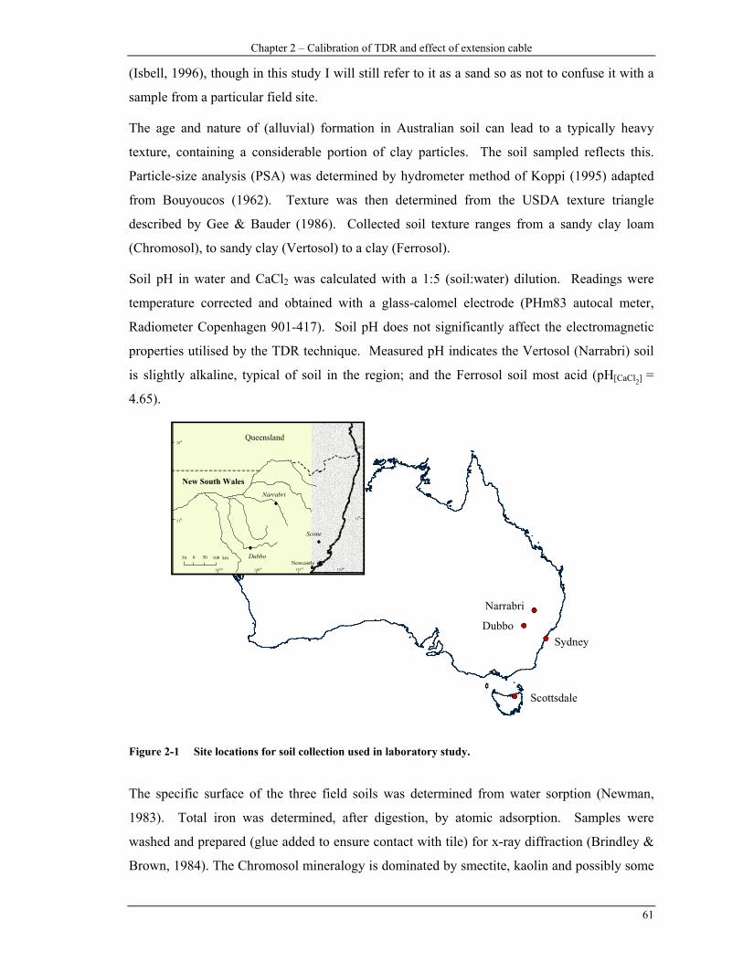
Chapter 2 – Calibration of TDR and effect of extension cable
61
(Isbell, 1996), though in this study I will still refer to it as a sand so as not to confuse it with a
sample from a particular field site.
The age and nature of (alluvial) formation in Australian soil can lead to a typically heavy
texture, containing a considerable portion of clay particles. The soil sampled reflects this.
Particle-size analysis (PSA) was determined by hydrometer method of Koppi (1995) adapted
from Bouyoucos (1962). Texture was then determined from the USDA texture triangle
described by Gee & Bauder (1986). Collected soil texture ranges from a sandy clay loam
(Chromosol), to sandy clay (Vertosol) to a clay (Ferrosol).
Soil pH in water and CaCl2 was calculated with a 1:5 (soil:water) dilution. Readings were
temperature corrected and obtained with a glass-calomel electrode (PHm83 autocal meter,
Radiometer Copenhagen 901-417). Soil pH does not significantly affect the electromagnetic
properties utilised by the TDR technique. Measured pH indicates the Vertosol (Narrabri) soil
is slightly alkaline, typical of soil in the region; and the Ferrosol soil most acid (pH[CaCl2] =
4.65).
Sydney
Narrabri
Dubbo
Scottsdale
50 0 50 100 km
28
31o
o
147 149 151 153
31
28
o
o
o oooNewcastle
New South Wales
Queensland
Narrabri
Dubbo
Scone
Figure 2-1 Site locations for soil collection used in laboratory study.
The specific surface of the three field soils was determined from water sorption (Newman,
1983). Total iron was determined, after digestion, by atomic adsorption. Samples were
washed and prepared (glue added to ensure contact with tile) for x-ray diffraction (Brindley &
Brown, 1984). The Chromosol mineralogy is dominated by smectite, kaolin and possibly some

B.H. George – Measuring soil water content
62
trace mica. A vermiculite chlorite integrade and kaolin dominate the Ferrosol mineralogy. And
the Vertosol soil is dominated by smectite and kaolin minerals.
Table 2-1 Soil physical characteristics for Chromosol, Vertosol, Ferrosol and a standard sand soil used
in TDR calibration and extension cable experiment.
Chromosol (Dubbo)
Vertosol (Narrabri)
Ferrosol (Scottsdale)
Sand (Parramatta)
Mean Std
Dev.
Mean Std
Dev.
Mean Std
Dev.
Mean Std
Dev.
Particle-size analysis % clay (< 0.002 mm)
32.88
2.556
37.01
1.640
47.55
0.471
% silt (0.002 - 0.02 mm) 10.73 1.746 12.53 0.970 18.48 0.299
% fine sand
(0.02 - 0.2 mm) 35.73 1.265 24.54 0.430 19.86 0.777
% coarse sand
(0.2 - 2.0 mm) 20.66 0.691 25.91 1.338 14.11 0.845
Texture Sandy clay
loam
Sandy clay Clay Sand
Organic Carbon (%) 1.57 0.06 0.91 0.03 2.78 0.62 0.05 0.07
pH [H2O] 6.64 8.14 5.12 6.38
pH [CaCl2] 5.55 7.35 4.65 4.81
Electrical conductivity
[1:5 H2O] (dS m-1)
1.96 0.017 2.43 0.021 2.47 0.036 0.18 0.022
Specific surface (m2 g-1) 397.4 8.45 375.2 4.24 304.3 5.12
Total Iron (%) 4.12 0.065 2.81 0.064 15.83 0.126 8.48
Number of samples 3 3 3 3 3
Organic carbon was determined with an adapted Walkley & Black (1934) method. The
organic carbon value is typical for Chromosol soil (Spain et al., 1993) indicating applied
effluent has not changed soil organic carbon significantly in the first two years of effluent
application. Intuitively, we expect greater organic carbon values due to the application of the
nutrient-rich effluent. However, small organic carbon values (1.57 %) are similar to other
values in an irrigated plantation in southern NSW (Falkiner & Smith, 1997). This could be due

Chapter 2 – Calibration of TDR and effect of extension cable
63
to the continued wetting and drying cycles created with application of effluent irrigation
(Polglase et al.,1995). Organic carbon is very small (0.05 %) in the sand and as expected, the
largest organic carbon values (2.78 %) obtained for the Ferrosol soil. These values are typical
of Ferrosol soil types (Spain et al., 1993).
Electrical conductivity is a major consideration in effectively determining maximum length of
TDR probe (Dalton, 1992) and is often a limiting factor in efficient TDR use. To maximise the
opportunities to obtain readings, 200 mm probes are utilised. A 1:5 extract of soil in water was
utilised to determine the electrical conductivity, with filtered samples analysed with a
temperature corrected conductivity meter (Radiometer Copenhagen DMN83).
2.3.2 Equipment
2.3.2.1 Time-domain reflectometers
To assess if the extension cable length was instrument-dependent or problematic of the TDR
technique, two instruments were utilised. A TRASE® System I TDR (Soilmoisture Equipment
Corporation Inc.; Santa Barbara CA, USA) and a Tektronix 1502B/C metallic cable tester
(Tektronix; Beaverton OR, USA) with Pyelab software (CSIRO Environmental Mechanics;
Canberra ACT, Australia) were used to measure Ka and determine θ. Technical specifications
for the time-domain reflectometry instruments are given in Table 2-2. Both instruments run
from internal and external power sources depending on battery status. Extension cables were
connected directly to the Bayonet Nelson Connector (BNC) on the measuring instrument.
Both TDR systems use automatic algorithms to report Ka to simplify measurement and to
minimise error in predicted θ (Timlin & Pachepsky, 1996).
2.3.2.2 Probes and extension cables
Two unbalanced probes from Soilmoisture Equipment Corporation (6000l20) were embedded
50 mm from the bottom of the soil in each of the tension columns. Probes were installed
during packing of the columns to ensure thorough contact with the soil and end-effects were
minimised by siting the probes at least 20 mm from the side of the tension table as shown in
Figure 2-2. The SEC probes are 200 mm in length with wire diameter of 3 mm and nominal
wire spacing of 25 mm. The critical spacing between wires should be three times (or more)
greater than the diameter of the centre wire (Zegelin et al., 1992). The SEC probes (25 mm /3
mm ≈ 8) therefore should not suffer from a “skin effect” as described by Knight (1992). A 2 m
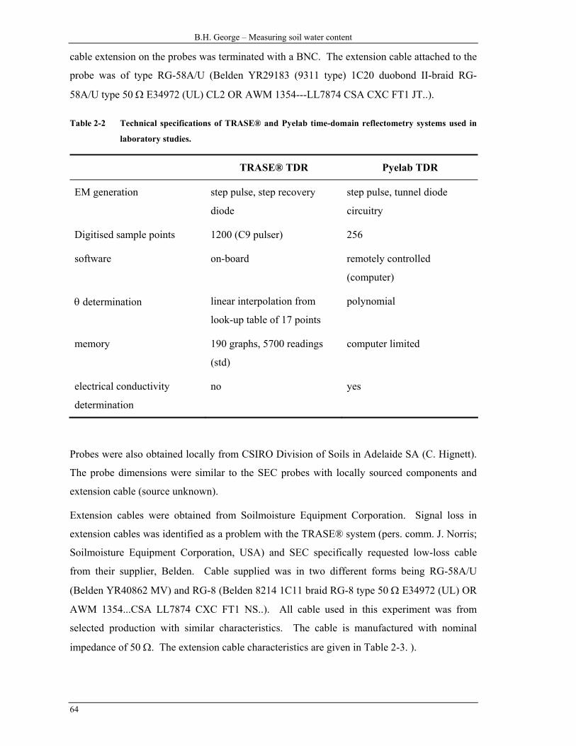
B.H. George – Measuring soil water content
64
cable extension on the probes was terminated with a BNC. The extension cable attached to the
probe was of type RG-58A/U (Belden YR29183 (9311 type) 1C20 duobond II-braid RG-
58A/U type 50 Ω E34972 (UL) CL2 OR AWM 1354---LL7874 CSA CXC FT1 JT..).
Table 2-2 Technical specifications of TRASE® and Pyelab time-domain reflectometry systems used in
laboratory studies.
TRASE® TDR Pyelab TDR
EM generation step pulse, step recovery
diode
step pulse, tunnel diode
circuitry
Digitised sample points 1200 (C9 pulser) 256
software on-board remotely controlled
(computer)
θ determination linear interpolation from
look-up table of 17 points
polynomial
memory 190 graphs, 5700 readings
(std)
computer limited
electrical conductivity
determination
no yes
Probes were also obtained locally from CSIRO Division of Soils in Adelaide SA (C. Hignett).
The probe dimensions were similar to the SEC probes with locally sourced components and
extension cable (source unknown).
Extension cables were obtained from Soilmoisture Equipment Corporation. Signal loss in
extension cables was identified as a problem with the TRASE® system (pers. comm. J. Norris;
Soilmoisture Equipment Corporation, USA) and SEC specifically requested low-loss cable
from their supplier, Belden. Cable supplied was in two different forms being RG-58A/U
(Belden YR40862 MV) and RG-8 (Belden 8214 1C11 braid RG-8 type 50 Ω E34972 (UL) OR
AWM 1354...CSA LL7874 CXC FT1 NS..). All cable used in this experiment was from
selected production with similar characteristics. The cable is manufactured with nominal
impedance of 50 Ω. The extension cable characteristics are given in Table 2-3. ).
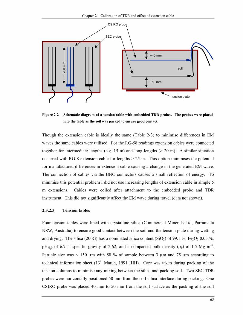
Chapter 2 – Calibration of TDR and effect of extension cable
65
+50 mm
+40 mm
soil
tension plate
CSIRO probe
SEC probe
200
mm
Figure 2-2 Schematic diagram of a tension table with embedded TDR probes. The probes were placed
into the table as the soil was packed to ensure good contact.
Though the extension cable is ideally the same (Table 2-3) to minimise differences in EM
waves the same cables were utilised. For the RG-58 readings extension cables were connected
together for intermediate lengths (e.g. 15 m) and long lengths (> 20 m). A similar situation
occurred with RG-8 extension cable for lengths > 25 m. This option minimises the potential
for manufactured differences in extension cable causing a change in the generated EM wave.
The connection of cables via the BNC connectors causes a small reflection of energy. To
minimise this potential problem I did not use increasing lengths of extension cable in simple 5
m extensions. Cables were coiled after attachment to the embedded probe and TDR
instrument. This did not significantly affect the EM wave during travel (data not shown).
2.3.2.3 Tension tables
Four tension tables were lined with crystalline silica (Commercial Minerals Ltd, Parramatta
NSW, Australia) to ensure good contact between the soil and the tension plate during wetting
and drying. The silica (200G) has a nominated silica content (SiO2) of 99.1 %; Fe2O3 0.05 %;
pHH20 of 6.7; a specific gravity of 2.62; and a compacted bulk density (ρb) of 1.5 Mg m-3.
Particle size was < 150 µm with 88 % of sample between 3 µm and 75 µm according to
technical information sheet (13th March, 1991 IHH). Care was taken during packing of the
tension columns to minimise any mixing between the silica and packing soil. Two SEC TDR
probes were horizontally positioned 50 mm from the soil-silica interface during packing. One
CSIRO probe was placed 40 mm to 50 mm from the soil surface as the packing of the soil
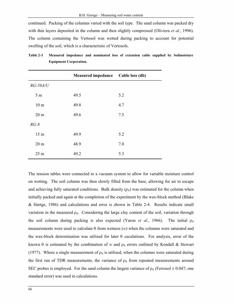
B.H. George – Measuring soil water content
66
continued. Packing of the columns varied with the soil type. The sand column was packed dry
with thin layers deposited in the column and then slightly compressed (Oliviera et al., 1996).
The column containing the Vertosol was wetted during packing to account for potential
swelling of the soil, which is a characteristic of Vertosols.
Table 2-3 Measured impedance and nominated loss of extension cable supplied by Soilmoisture
Equipment Corporation.
Measured impedance Cable loss (db)
RG-58A/U
5 m 49.5 5.2
10 m 49.8 4.7
20 m 49.6 7.5
RG-8
15 m 49.9 5.2
20 m 48.9 7.0
25 m 49.2 5.3
The tension tables were connected to a vacuum system to allow for variable moisture control
on wetting. The soil column was then slowly filled from the base, allowing for air to escape
and achieving fully saturated conditions. Bulk density (ρb) was estimated for the column when
initially packed and again at the completion of the experiment by the wax-block method (Blake
& Hartge, 1986) and calculations and error is shown in Table 2-4. Results indicate small
variation in the measured ρb. Considering the large clay content of the soil, variation through
the soil column during packing is also expected (Yaron et al., 1966). The initial ρb
measurements were used to calculate θ from wetness (w) when the columns were saturated and
the wax-block determination was utilised for later θ caculations. For analysis, error of the
known θ is estimated by the combination of w and ρb errors outlined by Kendall & Stewart
(1977). Where a single measurement of ρb is utilised, when the columns were saturated during
the first run of TDR measurements, the variance of ρb from repeated measurements around
SEC probes is employed. For the sand column the largest variance of ρb (Ferrosol ± 0.047; one
standard error) was used in calculations.

Chapter 2 – Calibration of TDR and effect of extension cable
67
Table 2-4 ρb measured by total column dimensions prior to TDR measurements and the (post TDR
measurements) wax-block method. One standard error in determination is given.
Sand Chromosol Ferrosol Vertosol
Dimensions (L×W×H, m) 0.326 × 0.326
× 0.140
0.348 × 0.350
× 0.175
0.349 × 0.351
× 0.167
0.349 × 0.350
× 0.185
Packed volume (m3) 0.01488 0.02131 0.02045 0.02324
Packed dry mass (kg) 18.5 24.4 23.0 25.6
Estimated ρb (Mg m-3) 1.42 1.15 1.09 1.10
Wax-block determination CSIRO probes not determined 1.40 (± 0.093) 1.34 (± 0.037) 1.42 (± 0.147)
SEC probes not determined 1.41 (± 0.026) 1.28 (± 0.022) 1.38 (± 0.063)
Average wax-block ρb not determined 1.40 (± 0.055) 1.29 (± 0.043) 1.40 (± 0.097)
2.3.3 Measurements and determination of Ka
To obtain readings during a “run” the TRASE® TDR and Pyelab TDR were positioned near
the tension table and the buried unbalanced probes connected directly to the respective
instrument. Prior to each reading, a waveform from step-generation to well past inflection was
taken and stored as a check on cable connections and general conditions. For each reported
reading three measurements were taken and averaged in a similar fashion to Rothe et al.
(1997). All measurements with the Pyelab TDR graphs were saved and one of the three
readings saved as a graph with the TRASE® TDR. Information was automatically stored on a
personal computer with the Pyelab TDR. Collected information on the TRASE® TDR was
transferred to the personal computer via Terminal (© Microsoft, 1993) and information
inspected with WinTRASE® (V1.11, beta test copy, © SEC and Jibray Inc).
After initial readings, different lengths of extension cable were inserted between the TDR
instrument and the unbalanced probe embedded in the column. Again, triplicate readings were
taken with each unbalanced probe and extension cable combination. The RG-58 cable
readings were taken with cable combinations of: 0 m (connected to probe with 2 m cable), 5 m,
10m, 15 m, 20 m, 25 m, 30 m, and 35 m. The actual length of extension becomes x + 2 m as
each probe has a 2 m cable from the end of the unbalanced probes to the BNC. Readings were
limited to 35 m. The recommended maximum RG-58 extension cable length for the TRASE®

B.H. George – Measuring soil water content
68
TDR is 30 m. Readings with the RG-8 cable reflected likely current usage. The RG-8 cable,
with a heavier shield and supposed lower signal loss characteristics was recommended for
longer extensions, especially with the C9 pulser in the TRASE® TDR system. The RG-8 cable
was used in combination lengths of: 15 m, 20 m, 25 m, 30 m, 35 m, 40 m, 45 m, and 60 m.
The columns were situated in a temperature-controlled room with readings taken at equilibrium
temperature near 20 °C (18 °C – 22 °C). Initial readings measured Ka when the soil in the
tension columns was totally saturated. The columns were then air-dried over several weeks
and returned to the temperature-controlled room for at least one-week before the measurements
were repeated. All readings recorded the travel time (t) of the EM wave along the probes
embedded in the soil.
2.4 RESULTS AND DISCUSSION
2.4.1 Comparison of reported θ by TDR instruments to known θ
Reported moisture content (θ) is the soil parameter we are normally interested in measuring
with the TDR technique. A comparison of reported θ by the TRASE® TDR and Pyelab TDR
systems to known moisture content (Kθ) is shown in Figure 2-3 where the reported TDR θ is
regressed against Kθ. There is a significant difference between the Kθ and measured θ (p =
0.05) for the TRASE® (p < 0.01) and Pyelab (p < 0.05) TDR systems. Linear regression
indicates a good fit of relationship (r2 = 0.984) for the Pyelab TDR system (Pθ) and a similar
result (r2 = 0.952) for the TRASE® TDR system (Tθ). However, if the data from the
Chromosol (when saturated) is excluded, the results of comparing the measured θ to Kθ are not
significantly different. One explanation for this is the error in estimation of ρb when the
columns were saturated. Also, the results indicate a sensitivity in the relationship possibly due
to the limited data set compared to others (Malicki et al., 1996; Yu et al., 1997).
Error in measured θ and Kθ was estimated for all probes at smaller and larger moisture
contents. The largest standard error of the mean (0.0084 m3 m-3) was calculated for SEC probe
(no. 4) embedded in the Vertosol at the lower Kθ of 0.153 m3 m-3. Other values were
consistently lower than 0.003 m3 m-3 indicating little error in the determination of θ from
repeated samples. Standard errors reported by the two TDR systems were also very small,
generally less than 0.001 m3 m-3. This is due to the repeatability of the TDR technique and
measurements recorded (n = 10) in calibration.
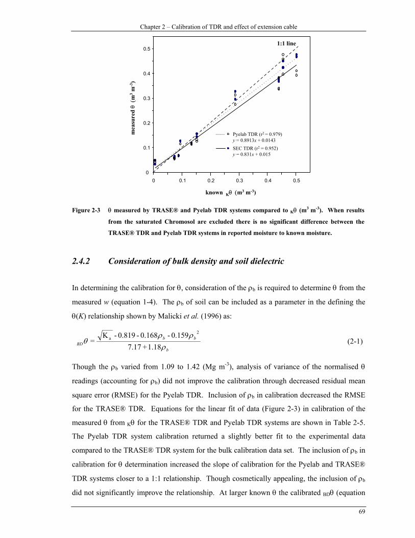
Chapter 2 – Calibration of TDR and effect of extension cable
69
1:1 line
Pyelab TDR (r2 = 0.979)y = 0.8913x + 0.0143SEC TDR (r2 = 0.952)y = 0.831x + 0.015
0
0.1
0.2
0.3
0.4
0.5
0 0.1 0.2 0.3 0.4 0.5
known Kθ (m3 m-3)
mea
sure
d θ
(m3 m
-3)
Figure 2-3 θ measured by TRASE® and Pyelab TDR systems compared to Kθ (m3 m-3). When results
from the saturated Chromosol are excluded there is no significant difference between the
TRASE® TDR and Pyelab TDR systems in reported moisture to known moisture.
2.4.2 Consideration of bulk density and soil dielectric
In determining the calibration for θ, consideration of the ρb is required to determine θ from the
measured w (equation 1-4). The ρb of soil can be included as a parameter in the defining the
θ(K) relationship shown by Malicki et al. (1996) as:
b
bbBD ρ
ρρθ
1.18+7.170.159-0.168-0.819-K
=2
a (2-1)
Though the ρb varied from 1.09 to 1.42 (Mg m-3), analysis of variance of the normalised θ
readings (accounting for ρb) did not improve the calibration through decreased residual mean
square error (RMSE) for the Pyelab TDR. Inclusion of ρb in calibration decreased the RMSE
for the TRASE® TDR. Equations for the linear fit of data (Figure 2-3) in calibration of the
measured θ from Kθ for the TRASE® TDR and Pyelab TDR systems are shown in Table 2-5.
The Pyelab TDR system calibration returned a slightly better fit to the experimental data
compared to the TRASE® TDR system for the bulk calibration data set. The inclusion of ρb in
calibration for θ determination increased the slope of calibration for the Pyelab and TRASE®
TDR systems closer to a 1:1 relationship. Though cosmetically appealing, the inclusion of ρb
did not significantly improve the relationship. At larger known θ the calibrated BDθ (equation
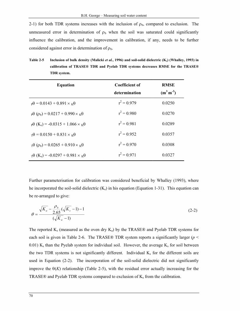
B.H. George – Measuring soil water content
70
2-1) for both TDR systems increases with the inclusion of ρb, compared to exclusion. The
unmeasured error in determination of ρb when the soil was saturated could significantly
influence the calibration, and the improvement in calibration, if any, needs to be further
considered against error in determination of ρb.
Table 2-5 Inclusion of bulk density (Malicki et al., 1996) and soil-solid dielectric (Ks) (Whalley, 1993) in
calibration of TRASE® TDR and Pyelab TDR systems decreases RMSE for the TRASE®
TDR system.
Equation Coefficient of
determination
RMSE
(m3 m-3)
Pθ = 0.0143 + 0.891 × Kθ r2 = 0.979 0.0250
Pθ (ρb) = 0.0217 + 0.990 × Kθ r2 = 0.980 0.0270
Pθ (Ks) = -0.0315 + 1.066 × Kθ r2 = 0.981 0.0289
Tθ = 0.0150 + 0.831 × Kθ r2 = 0.952 0.0357
Tθ (ρb) = 0.0265 + 0.910 × Kθ r2 = 0.970 0.0308
Tθ (Ks) = -0.0297 + 0.981 × Kθ r2 = 0.971 0.0327
Further parameterisation for calibration was considered beneficial by Whalley (1993), where
he incorporated the soil-solid dielectric (Ks) in his equation (Equation 1-31). This equation can
be re-arranged to give:
)1(
1)1(65.2
−
−−−=
w
sb
a
K
KKρ
θ (2-2)
The reported Ks (measured as the oven dry Ka) by the TRASE® and Pyelab TDR systems for
each soil is given in Table 2-6. The TRASE® TDR system reports a significantly larger (p <
0.01) Ks than the Pyelab system for individual soil. However, the average Ks for soil between
the two TDR systems is not significantly different. Individual Ks for the different soils are
used in Equation (2-2). The incorporation of the soil-solid dielectric did not significantly
improve the θ(K) relationship (Table 2-5), with the residual error actually increasing for the
TRASE® and Pyelab TDR systems compared to exclusion of Ks from the calibration.

Chapter 2 – Calibration of TDR and effect of extension cable
71
Table 2-6 Measured soil-solid dielectric (Ks) of the oven-dry soil (105 °C for 24 hours) with the
TRASE® TDR and Pyelab TDR systems. θ is the reported moisture content from the
respective TDR system with associated error.
Soil TRASE® TDR Pyelab TDR
Ks (-) θ (m3 m-3) Ks (-) θ (m3 m-3)
Sand 2.7 (± 0.0) 0.0188
(± 0.00042)
2.57 (± 0.036) 0.0182
(± 0.0007)
Chromosol 2.59 (± 0.032) 0.0154
(± 0.00052)
2.40 (± 0.019) 0.0141
(± 0.00032)
Vertosol 2.6 (± 0.0) 0.0156
(± 0.00052)
2.47 (± 0.023) 0.0156
(± 0.00084)
Ferrosol 2.82 (± 0.042) 0.0228
(± 0.00063)
2.72 (± 0.036) 0.0226
(± 0.00126)
Average 2.68 (± 0.097) 2.54 (± 0.128)
2.4.3 Comparison of θ reported by TRASE® TDR and Pyelab TDR systems
The mean reported θ (n = 10) from the Pyelab TDR system for all soil types at saturated and
air-dry conditions is plotted against the reported θ for the TRASE® TDR system (Figure 2-4).
A paired t-test (p = 0.05) indicates no significant difference between the two TDR systems
(also not significantly different from the 1:1 line).
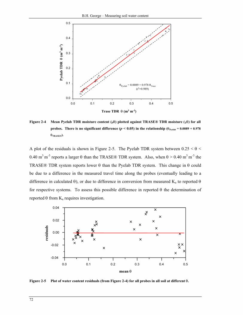
B.H. George – Measuring soil water content
72
Trase TDR θ (m3 m-3)
Pyel
ab T
DR
θ (m
3 m-3
)
0.0
0.1
0.2
0.3
0.4
0.5
0.0 0.1 0.2 0.3 0.4 0.5
θPyelab = 0.0089 + 0.978 θTrase(r2=0.989)
Figure 2-4 Mean Pyelab TDR moisture content (Pθ) plotted against TRASE® TDR moisture (Tθ) for all
probes. There is no significant difference (p < 0.05) in the relationship (θPyelab = 0.0089 + 0.978
θTRASE®).
A plot of the residuals is shown in Figure 2-5. The Pyelab TDR system between 0.25 < θ <
0.40 m3 m-3 reports a larger θ than the TRASE® TDR system. Also, when θ > 0.40 m3 m-3 the
TRASE® TDR system reports lower θ than the Pyelab TDR system. This change in θ could
be due to a difference in the measured travel time along the probes (eventually leading to a
difference in calculated θ), or due to difference in conversion from measured Ka to reported θ
for respective systems. To assess this possible difference in reported θ the determination of
reported θ from Ka requires investigation.
-0.04
-0.02
0.00
0.02
0.04
0.0 0.1 0.2 0.3 0.4 0.5
mean θ
resi
dua l
s
Figure 2-5 Plot of water content residuals (from Figure 2-4) for all probes in all soil at different θ.
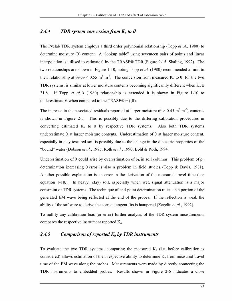
Chapter 2 – Calibration of TDR and effect of extension cable
73
2.4.4 TDR system conversion from Ka to θ
The Pyelab TDR system employs a third order polynomial relationship (Topp et al., 1980) to
determine moisture (θ) content. A “lookup table” using seventeen pairs of points and linear
interpolation is utilised to estimate θ by the TRASE® TDR (Figure 9-15; Skaling, 1992). The
two relationships are shown in Figure 1-10, noting Topp et al. (1980) recommended a limit to
their relationship at θTOPP < 0.55 m3 m-3. The conversion from measured Ka to θ, for the two
TDR systems, is similar at lower moisture contents becoming significantly different when Ka ≥
31.8. If Topp et al.’s (1980) relationship is extended it is shown in Figure 1-10 to
underestimate θ when compared to the TRASE® θ (Tθ).
The increase in the associated residuals reported at larger moisture (θ > 0.45 m3 m-3) contents
is shown in Figure 2-5. This is possibly due to the differing calibration procedures in
converting estimated Ka to θ by respective TDR systems. Also both TDR systems
underestimate θ at larger moisture contents. Underestimation of θ at larger moisture content,
especially in clay textured soil is possibly due to the change in the dielectric properties of the
“bound” water (Dobson et al., 1985; Roth et al., 1990; Bohl & Roth, 1994
Underestimation of θ could arise by overestimation of ρb in soil columns. This problem of ρb
determination increasing θ error is also a problem in field studies (Topp & Davis, 1981).
Another possible explanation is an error in the derivation of the measured travel time (see
equation 1-18.). In heavy (clay) soil, especially when wet, signal attenuation is a major
constraint of TDR systems. The technique of end-point determination relies on a portion of the
generated EM wave being reflected at the end of the probes. If the reflection is weak the
ability of the software to derive the correct tangent fits is hampered (Zegelin et al., 1992).
To nullify any calibration bias (or error) further analysis of the TDR system measurements
compares the respective instrument reported Ka.
2.4.5 Comparison of reported Ka by TDR instruments
To evaluate the two TDR systems, comparing the measured Ka (i.e. before calibration is
considered) allows estimation of their respective ability to determine Ka from measured travel
time of the EM wave along the probes. Measurements were made by directly connecting the
TDR instruments to embedded probes. Results shown in Figure 2-6 indicates a close

B.H. George – Measuring soil water content
74
relationship between Ka measured by the TRASE® TDR compared to the Pyelab TDR system.
There is a high correlation (r = 0.996) between readings with the relationship estimated by:
PKa = -0.0828 + 1.037 × TKa (2-3)
again with an expected good fit (r2 = 0.992). There is no significant difference between the two
slopes or the two intercepts (p < 0.05). This indicates that the TDR systems report a similar
measured Ka and reported differences are then in determination of θ from Ka (i.e. estimated
calibration algorithms).
Trase TDR Ka
Pyel
ab T
DR
Ka
5
10
15
20
25
30
35
5 10 15 20 25 30
95% density ellipse
Pyelab Ka = -0.0828 + 1.037TRASE Ka(r2 = 0.992)
Figure 2-6 Regression of Ka determined by Pyelab TDR and TRASE® TDR systems. The relationship
(equation 2-3) shows no significant difference between the reported Ka by the TRASE® and
Pyelab TDR systems.
2.4.6 Calibration of Pyelab and TRASE® TDR systems
A preferred calibration involves the physically based relationship between the measured
refractive index (√Κa) plotted against the Kθ. The √Κa is the square root of the measured Ka
(Section 1.5.6) and several researchers, e.g. Herkelrath et al., (1991); Whalley (1993); and
Malicki et al., (1996) have employed the relationship in calibration of the TDR technique in
different soil. Figure 2-7 shows the calculated calibration for the TRASE® TDR and Pyelab
TDR systems. A significant difference between the TRASE® TDR and Pyelab TDR slopes
obtained in calibration exists (p < 0.01; t = 7.23, 40 d.f). The determination of √Κa from the

Chapter 2 – Calibration of TDR and effect of extension cable
75
Pyelab and TRASE® TDR systems yield similar relationships to that of Topp et al. (1980)
when their equation (1-24) is formulated (where θ < 0.45 m3 m-3).
P√Κa = 1.625 + 7.941 Kθ (2-4)
T√Κa = 1.663 + 7.265 Kθ (2-5)
Topp√Κa = 1.531 + 8.629 Kθ (2-6)
Though not incorporating the parameters of the mixing model approach, results are similar to
those of Alharti & Lange (1987) and Lediu et al. (1986), especially where moisture content is
small. The slope of the calibrations is lower than those reported by Lediu et al. (1986),
possibly due to the limited soil types in calibration with large clay contents. Also, the ρb
determination was not accounted for following comparison to Malicki et al.’s (1996) work
considering the potential limitations in ρb determination, especially when the soil was
saturated.
0
1
2
3
4
5
0 0.1 0.2 0.3 0.4 0.5
Pyelab TDR √Ka = 7.535θ + 1.677 (r2 = 0.979)
Trase TDR √Ka = 6.823θ + 1.730 (r2 = 0.947)
Topp et al. (1980)
known θ (m3 m-3)
refr
activ
e in
dex
(√ K
a)
Figure 2-7 Linear relationship for calibration of measured refractive index (√Ka) against the known
moisture content (Kθ) for the TRASE® and Pyelab TDR systems. At higher moisture
contents both TDR systems report a lower √Ka compared to (the re-arranged) Topp et al.’s
(1980) “universal” calibration.
Figure 2-7 shows the Pyelab TDR system returning larger Ka values compared to the TRASE®
TDR system at larger moisture contents. Returning to Figure 2-3 this difference is masked by
the system calibration procedures at larger moisture contents where the TRASE® calibration

B.H. George – Measuring soil water content
76
will yield a larger θ compared to the derivation (via Topp et al. (1980) equation) of θ with the
Pyelab TDR system at the same measured Ka.
After calibration we are interested in obtaining θ from the calculated Ka. The straight-line
calibration curve is the inverse of the initial regression in the form:
x y ab
=−( ) (2-6)
in this case
baK a )( −
=θ (2-7)
where a is the intercept, b the slope and √Ka the refractive index. The error associated with the
inverse estimation (prediction) in calibration requires more detailed consideration (Webster,
1997). The variance in determination of Kθ (for determined √Ka against θ) is much less than
the sum of the difference between the observed value (xi) and the centroid (x ) and the
confidence limits (l) for the calibration can be determined:
l x tsb n
x x
x xo
o
i
= ± + +−
−∑
1 1
2
2
_
_ (2-8)
where xo is the predicted variable (θ); t is the Students t (1.7250.05,20 in this case); s is the square
root of the variance (of Y,x); b is the slope (of Y,x); and n is the number of observations in
calibration (22 known moisture contents). The two calibration curves for the TRASE® TDR
and Pyelab systems including error of prediction is shown in Figure 2-8.
Estimation of θ from measured Ka with the Pyelab TDR system is determined by:
estPθ = 0.1259√Ka - 0.2045 (± 0.054 m3 m-3) (2-9)
To estimate the θ from a measured Ka with the TRASE® TDR the equation is:
estTθ = 0.1376√Ka - 0.2289 (± 0.062 m3 m-3) (2-10)
The error in determination of θ from measured Ka is larger than that obtained by Topp et al.
(1980) in an empirical calibration encompassing ρb and temperature for mineral soil (two
standard errors ± 0.026 m3 m-3). Also, Skaling (1992) indicates an error of ± 0.02 m3 m-3 for
the TRASE® TDR in calibration.
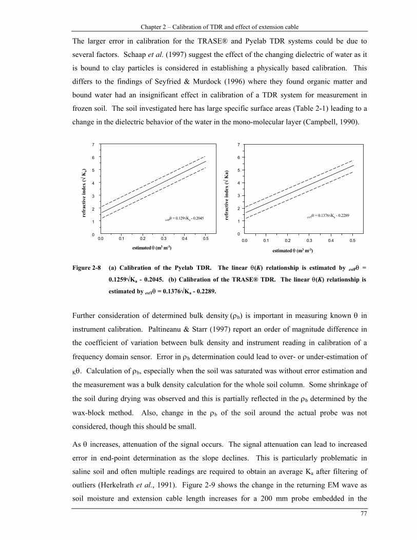
Chapter 2 – Calibration of TDR and effect of extension cable
77
The larger error in calibration for the TRASE® and Pyelab TDR systems could be due to
several factors. Schaap et al. (1997) suggest the effect of the changing dielectric of water as it
is bound to clay particles is considered in establishing a physically based calibration. This
differs to the findings of Seyfried & Murdock (1996) where they found organic matter and
bound water had an insignificant effect in calibration of a TDR system for measurement in
frozen soil. The soil investigated here has large specific surface areas (Table 2-1) leading to a
change in the dielectric behavior of the water in the mono-molecular layer (Campbell, 1990).
0
1
2
3
4
5
6
7
0.0 0.1 0.2 0.3 0.4 0.5
estimated θ (m3 m-3)
refr
activ
e in
dex
(√ K
a)
estPθ = 0.129√Ka - 0.2045
estimated θ (m3 m-3)
refr
activ
e in
dex
(√ K
a)0
1
2
3
4
5
6
7
0.0 0.1 0.2 0.3 0.4 0.5
estTθ = 0.1376√Ka - 0.2289
Figure 2-8 (a) Calibration of the Pyelab TDR. The linear θ(K) relationship is estimated by estPθ =
0.1259√Ka - 0.2045. (b) Calibration of the TRASE® TDR. The linear θ(K) relationship is
estimated by estTθ = 0.1376√Ka - 0.2289.
Further consideration of determined bulk density (ρb) is important in measuring known θ in
instrument calibration. Paltineanu & Starr (1997) report an order of magnitude difference in
the coefficient of variation between bulk density and instrument reading in calibration of a
frequency domain sensor. Error in ρb determination could lead to over- or under-estimation of
Kθ. Calculation of ρb, especially when the soil was saturated was without error estimation and
the measurement was a bulk density calculation for the whole soil column. Some shrinkage of
the soil during drying was observed and this is partially reflected in the ρb determined by the
wax-block method. Also, change in the ρb of the soil around the actual probe was not
considered, though this should be small.
As θ increases, attenuation of the signal occurs. The signal attenuation can lead to increased
error in end-point determination as the slope declines. This is particularly problematic in
saline soil and often multiple readings are required to obtain an average Ka after filtering of
outliers (Herkelrath et al., 1991). Figure 2-9 shows the change in the returning EM wave as
soil moisture and extension cable length increases for a 200 mm probe embedded in the
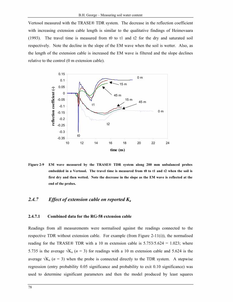
B.H. George – Measuring soil water content
78
Vertosol measured with the TRASE® TDR system. The decrease in the reflection coefficient
with increasing extension cable length is similar to the qualitative findings of Heimovaara
(1993). The travel time is measured from t0 to t1 and t2 for the dry and saturated soil
respectively. Note the decline in the slope of the EM wave when the soil is wetter. Also, as
the length of the extension cable is increased the EM wave is filtered and the slope declines
relative to the control (0 m extension cable).
-0.35
-0.3
-0.25
-0.2
-0.15
-0.1
-0.05
0
0.05
0.1
0.15
10 12 14 16 18 20 22 24
time (ns)
refle
ctio
n co
effic
ient
(-)
0 m
15 m
0 m
45 m15 m
45 m
t0
t1
t2
Figure 2-9 EM wave measured by the TRASE® TDR system along 200 mm unbalanced probes
embedded in a Vertosol. The travel time is measured from t0 to t1 and t2 when the soil is
first dry and then wetted. Note the decrease in the slope as the EM wave is reflected at the
end of the probes.
2.4.7 Effect of extension cable on reported Ka
2.4.7.1 Combined data for the RG-58 extension cable
Readings from all measurements were normalised against the readings connected to the
respective TDR without extension cable. For example (from Figure 2-11(i)), the normalised
reading for the TRASE® TDR with a 10 m extension cable is 5.753/5.624 = 1.023; where
5.735 is the average √Ka (n = 3) for readings with a 10 m extension cable and 5.624 is the
average √Ka (n = 3) when the probe is connected directly to the TDR system. A stepwise
regression (entry probability 0.05 significance and probability to exit 0.10 significance) was
used to determine significant parameters and then the model produced by least squares

Chapter 2 – Calibration of TDR and effect of extension cable
79
estimation (Figure 2-10). To explain 62.2 % of the variation a total of six parameters were
used: TDR system; TDR probe; cable length; standard error of measurements; clay content and
soil water content (either saturated or air dry). There is no clear relationship between
increasing cable extension and change (increase) in measured √Ka. To establish if there is a
relationship, further differentiation of the data set is considered in more detail.
0.95
1.00
1.05
1.10
1.15
1.20
.95 1.00 1.05 1.10 1.15 1.20
norm
alis
ed v
alue
predicted normal value
Figure 2-10 Model fit of normalised √Ka for all soil with RG-58 extension cable connections. The model
explains 62.2 % of the variation whilst accounting for interactions between soil type (as clay
%), cable length, TDR system, TDR probe, moisture conditions of the soil (saturated versus
air dry) and standard deviation of measurements. Cable length was not significant as a single
parameter.
2.4.7.2 Vertosol as an example
An example of determination of Ka (shown as √Ka, the refractive index) in a Vertosol with the
RG-58 extension cable attached to Soilmoisture Equipment Corporation (SEC) unbalanced
probes and locally produced (CSIRO, Adelaide) probes is shown in Figure 2-11. Further
results for individual soil types are shown in Appendix 2-1.

B.H. George – Measuring soil water content
80
5.57
5.62
5.67
5.72
5.77
5.82
5.87
0 05 10 15 20 25 30 35 All Pairs With Control
refr
activ
e in
dex
(√K
a)
cable length (m) (i)
5.60
5.70
5.80
5.90
6.00
6.10
6.20
6.30
6.40
0 05 10 15 20 All Pairs With Control
refr
activ
e in
dex
(√K
a)
cable length (m) (i)
5.53
5.58
5.63
5.67
5.72
5.77
5.82
0 05 10 15 20 30 All Pairs With Control
refr
activ
e in
dex
(√K
a)
cable length (m)25
(ii)
Figure 2-11 TRASE® TDR determination of Ka in
a saturated Vertosol. (i) is a Soilmoisture
Equipment unbalanced probe, (ii) CSIRO
unbalanced probe. The TRASE® TDR did not
determine the end-point of the reflected EM
wave for the 35 m extension cable.
5.50
5.75
6.00
6.25
6.50
6.75
7.00
7.25
7.50
0 05 10 15 20 All Pairs With Control
refr
activ
e in
dex
(√K
a)
cable length (m)
(ii)
Figure 2-12 Pyelab TDR determination of Ka in a
saturated Vertosol. (i) is a Soilmoisture
Equipment unbalanced probe, (ii) CSIRO
unbalanced probe. The Pyelab TDR could not
determine the end-point of the reflected EM
wave for extension cable lengths greater than
20 m in the saturated Vertosol
A comparison of means test utilising the least significant difference (LSD) from a Tukey-
Kramer test indicates differences between triplicate readings. The Tukey-Kramer test is
preferred for multiple comparisons to minimise Type I errors (Carmer & Walker, 1982; SAS
Institute, 1995). Visually this is interpreted as significant difference in √Ka where the angle of
intersection between overlapping circles is < 90°. Also where circles do not overlap at all a
significant difference in the measured √Ka is expected. The control is determined as the
measured √Ka when the probe is connected directly to the respective TDR system. To estimate

Chapter 2 – Calibration of TDR and effect of extension cable
81
if reported √Ka is significantly different from the control (0) a Dunnett’s test (again using the
protected LSD at a 5 % significance level) is conducted (SAS Institute, 1995).
2.58
2.68
2.78
2.88
2.98
3.08
0 5 10 15 20 25 30 35 All Pairs With Control
cable length (m)
refr
activ
e in
dex
(√K
a)
(i)
2.50
2.60
2.70
2.80
2.90
3.00
3.10
3.20
3.30
0 5 10 15 20 30 35 All Pairs With Control
cable length (m)
refr
activ
e in
dex
(√K
a)
(i)
2.55
2.65
2.75
2.85
2.95
0 05 10 15 20 25 30 35 All Pairs With Control
cable length (m)
refr
activ
e in
dex
(√K
a)
(ii)
Figure 2-13 TRASE® TDR determination of Ka in
an air-dry Vertosol. Measurements are taken
with 200 mm long probes attached to varying
length RG-58 cable. (i) is a SEC unbalanced
probe, (ii) CSIRO unbalanced probe. The
TRASE® TDR did not determine the end-point
of the reflected EM wave for the 35 m
extension cable.
2.50
2.60
2.70
2.80
2.90
3.00
3.10
3.20
0 05 10 15 20 25 30 35 All Pairs With Control
cable length (m)
refr
activ
e in
dex
(√K
a)
(ii)
Figure 2-14 Pyelab TDR determination of Ka in an
air-dry Vertosol. Measurements are taken
with 200 mm long probes attached to varying
length RG-58 cable. (i) is a SEC unbalanced
probe, (ii) CSIRO unbalanced probe. The
Pyelab TDR could not determine the end-point
of the reflected EM wave for extension cable
lengths greater than 20 m in the saturated
Vertosol
Significant differences exist between the measured √Ka with the TRASE® TDR and Pyelab
TDR systems in saturated and unsaturated soil with both probes. Figures 2-11, 2-12, 2-13 and
2-14 show the differences between reported √Ka due to the addition of RG-58 extension cable.
Generally an increase in reported √Ka occurs as the extension cable length increases. When
the soil is saturated (Figure 2-11) the TRASE® TDR system obtained readings for all cable
lengths from 0 to 35 m extension. Results (Figure 2-12(i)) indicate a saw-tooth pattern with an

B.H. George – Measuring soil water content
82
increase in reported √Ka from the control (0 m) to 10 m, then no significant increase in
reported √Ka until 30 m and 35 m extension cables are employed. The CSIRO probe yielded a
different result (Figure 2-12(ii)). There was no significant difference in results with extension
cables of 5 m and 10 m length from the control. A difference exists with extension cables
greater then 10 m.
The TRASE® TDR and Pyelab TDR systems respond differently to increasing RG-58
extension cable. The SEC probe and CSIRO probes also respond differently to the changing
moisture conditions. These changes indicate the response to increasing extension cable length
is masked in the model (Figure 2-10) where 62.2 % of the variation is explained. Figure 2-15
and Figure 2-16 shows the modelled response of the increasing extension cable with the
different TDR systems, probes and moisture contents. In the saturated Vertosol the Pyelab
TDR and TRASE® TDR systems reported increasing refractive index (√Ka) with increasing
cable length. The linear relationship between the increasing extension cable length and √Ka is
shown in Figure 2-15. When the Vertosol was at smaller moisture conditions the Pyelab TDR
system still exhibited a linear response to increasing extension cable length. The TRASE®
TDR system response is better explained when the extension cable length is split at 15 m to 20
m (Figure 2-16(iii) and Figure 2-16(iv)). This could be due to the timing mechanism used by
the TRASE® TDR system and measurement of travel time at different cable lengths that affect
the Tektronix TDR systems (Hook & Livingston, 1995). Information on the time-base
mechanism used by the TRASE® TDR system is not available.
Analysis of the waveform (data not shown) indicates that the CSIRO probe yields a greater
spike (due to larger impedance) in the waveform on entering the soil. This assists in the
automatic determination of the start point of the EM wave and by increasing the energy
difference could improve the end-point determination in lossy soil, in this case a wet, large
specific surface area Vertosol. The increase in the reflection coefficient could also improve the
ability of the TDR software to determine the start point (Heimovaara, 1993). However, the
increased energy associated with the EM wave entering the soil also leads to greater loss of
energy and this reduces the ability of the TDR instrument to obtain a measurement due to
increased attenuation.
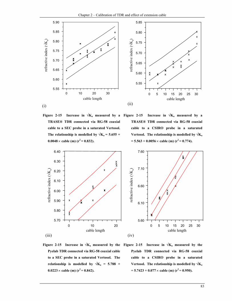
Chapter 2 – Calibration of TDR and effect of extension cable
83
5.55
5.60
5.65
5.70
5.75
5.80
5.85
5.90
0 10 20 30cable length
refr
activ
e in
dex
( √K
a)
(i)
cable length
refr
activ
e in
dex
( √K
a)
5.55
5.60
5.65
5.70
5.75
5.80
5.85
0 5 10 15 20 25 30
(ii)
Figure 2-15 Increase in √Ka measured by a
TRASE® TDR connected via RG-58 coaxial
cable to a SEC probe in a saturated Vertosol.
The relationship is modelled by √Ka = 5.655 +
0.0048 × cable (m) (r2 = 0.832).
Figure 2-15 Increase in √Ka measured by a
TRASE® TDR connected via RG-58 coaxial
cable to a CSIRO probe in a saturated
Vertosol. The relationship is modelled by √Ka
= 5.563 + 0.0056 × cable (m) (r2 = 0.774).
cable length
5.70
5.80
5.90
6.00
6.10
6.20
6.30
6.40
0 10 20
refr
activ
e in
dex
( √K
a)
(iii)
5.60
6.10
6.60
7.10
7.60
0 5 10 15 20 25 30cable length
refr
act iv
e in
dex
( √K
a)
(iv)
Figure 2-15 Increase in √Ka measured by the
Pyelab TDR connected via RG-58 coaxial cable
to a SEC probe in a saturated Vertosol. The
relationship is modelled by √Ka = 5.788 +
0.0223 × cable (m) (r2 = 0.842).
Figure 2-15 Increase in √Ka measured by the
Pyelab TDR connected via RG-58 coaxial
cable to a CSIRO probe in a saturated
Vertosol. The relationship is modelled by √Ka
= 5.7423 + 0.077 × cable (m) (r2 = 0.950).

B.H. George – Measuring soil water content
84
2.60
2.70
2.80
2.90
3.00
0 10 20 30cable length
refr
activ
e in
dex
( √K
a)(i)
2.60
2.65
2.70
2.75
2.80
2.85
2.90
2.95
5 10 15 20 25 30 35
cable length
refra
ctiv
e i n
dex
( √K
a)
(ii)
Figure 2-16 Increase in √Ka measured by the
TRASE® TDR connected via RG-58 coaxial
cable to a SEC probe in an air-dry Vertosol.
The relationship is modelled by √Ka = 2.6243 +
0.0113 × cable (m) (r2 = 0.891).
Figure 2-16 Increase in √Ka measured by the
TRASE® TDR connected via RG-58 coaxial
cable to a CSIRO probe in an air-dry
Vertosol. The relationship is modelled by √Ka
= 2.6058 + 0.0074 × cable (m) (r2 = 0.766).
2.60
2.70
2.80
2.90
3.00
0 10 20 30
cable length
refr
activ
e in
dex
( √K
a)
(iii)
2.60
2.65
2.70
2.75
2.80
2.85
2.90
2.95
5 10 15 20 25 30 35
cable length
refr
a ctiv
e in
d ex
( √K
a)
(iv)
Figure 2-16 Increase in √Ka measured by the
TRASE® TDR connected via RG-58 coaxial
cable to a SEC probe in an air-dry Vertosol. A
straight-line relationship for extension cable ≤
15 m is √Ka = 2.595 + 0.0181 × cable (m) (r2 =
0.994) and for RG-58 cable ≥ 20 m the
relationship is given by √Ka = 2.4071 + 0.0180
× cable (m) (r2 = 0.970).
Figure 2-16 Increase in √Ka measured by the
TRASE® TDR connected via RG-58 coaxial
cable to a CSIRO probe in an air-dry
Vertosol. A straight-line relationship for
extension cable ≤ 15 m √Ka = 2.5672 + 0.0136
× cable (m) (r2 = 0.948) and for RG-58 cable ≥
20 m the relationship is given by √Ka = 2.3895
+ 0.0147 × cable (m) (r2 = 0.997).
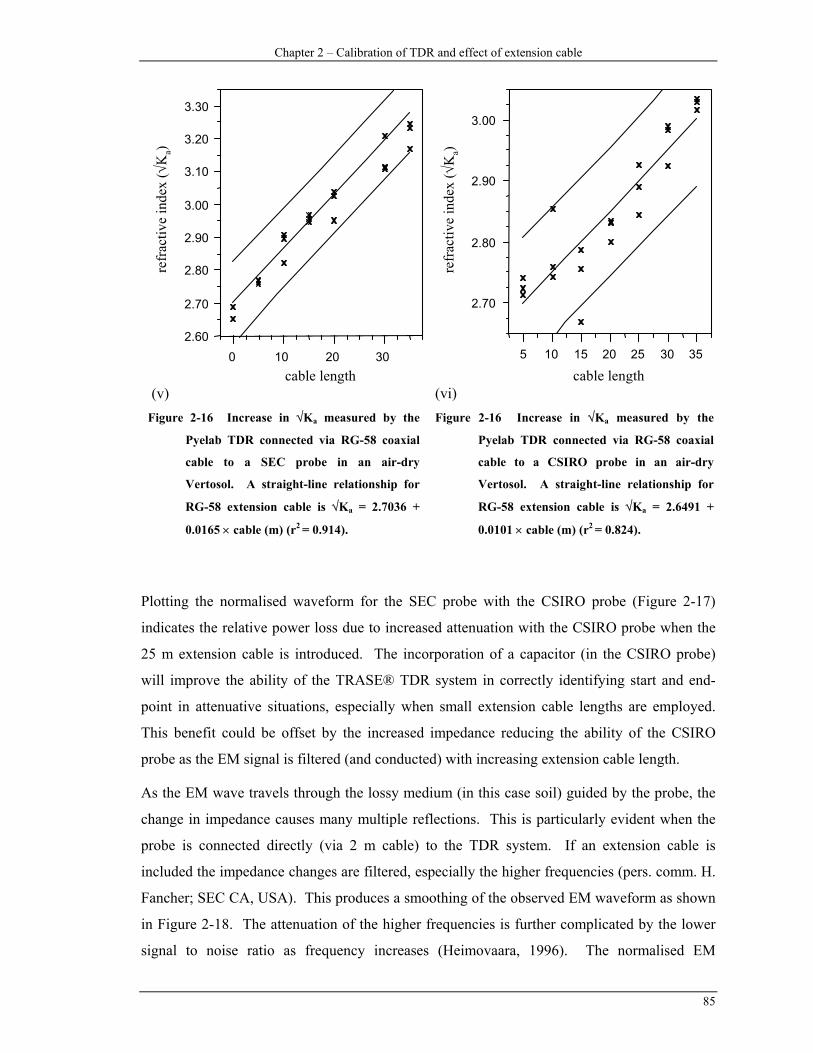
Chapter 2 – Calibration of TDR and effect of extension cable
85
2.60
2.70
2.80
2.90
3.00
3.10
3.20
3.30
0 10 20 30cable length
refr
a ctiv
e in
dex
( √K
a)
(v)
2.70
2.80
2.90
3.00
5 10 15 20 25 30 35
cable length
refr
activ
e in
dex
( √K
a)
(vi)
Figure 2-16 Increase in √Ka measured by the
Pyelab TDR connected via RG-58 coaxial
cable to a SEC probe in an air-dry
Vertosol. A straight-line relationship for
RG-58 extension cable is √Ka = 2.7036 +
0.0165 × cable (m) (r2 = 0.914).
Figure 2-16 Increase in √Ka measured by the
Pyelab TDR connected via RG-58 coaxial
cable to a CSIRO probe in an air-dry
Vertosol. A straight-line relationship for
RG-58 extension cable is √Ka = 2.6491 +
0.0101 × cable (m) (r2 = 0.824).
Plotting the normalised waveform for the SEC probe with the CSIRO probe (Figure 2-17)
indicates the relative power loss due to increased attenuation with the CSIRO probe when the
25 m extension cable is introduced. The incorporation of a capacitor (in the CSIRO probe)
will improve the ability of the TRASE® TDR system in correctly identifying start and end-
point in attenuative situations, especially when small extension cable lengths are employed.
This benefit could be offset by the increased impedance reducing the ability of the CSIRO
probe as the EM signal is filtered (and conducted) with increasing extension cable length.
As the EM wave travels through the lossy medium (in this case soil) guided by the probe, the
change in impedance causes many multiple reflections. This is particularly evident when the
probe is connected directly (via 2 m cable) to the TDR system. If an extension cable is
included the impedance changes are filtered, especially the higher frequencies (pers. comm. H.
Fancher; SEC CA, USA). This produces a smoothing of the observed EM waveform as shown
in Figure 2-18. The attenuation of the higher frequencies is further complicated by the lower
signal to noise ratio as frequency increases (Heimovaara, 1996). The normalised EM

B.H. George – Measuring soil water content
86
waveforms (Figure 2-18) show a decrease in the proportion of the EM wave returning along
the probes buried in the soil.
-0.35
-0.3
-0.25
-0.2
-0.15
-0.1
-0.05
0
0.05
10 12 14 16 18 20 22
SEC 0
CSIRO 0
CSIRO 25 m SEC 25 m
time (ns)
refle
ctio
n co
effic
ient
(-)
Figure 2-17 Normalised SEC probe and CSIRO probe measured with the TRASE® TDR for control and
25 m extension cable length. The TRASE® TDR did not pick the end-point for the 25 m
extension cable measured with the CSIRO probe.
-0.25
-0.2
-0.15
-0.1
-0.05
0
0.05
10 11 12 13 14 15 16 17 18 19
0 m5 m20 m
35 m
refle
ctio
n co
effic
ient
(-)
time (ns)
Figure 2-18 Normalised EM waveforms for the SEC probe measured with the TRASE® TDR system in
the saturated Vertosol for control, 5 m, 20 m and 35 m RG-58 extension cable. With
increasing extension cable there is a decrease in the energy of the returning EM wave and
corresponding decline in the slope of the reflected EM wave.

Chapter 2 – Calibration of TDR and effect of extension cable
87
Associated with a decrease in the energy of the returning EM wave is a decline in the measured
slope for start and end-point determination. This is readily observed when plotting voltage
versus time for different treatments (Figure 2-18). The determination of the slope is important,
as the automatic software regimes aim to determine the intersection of the two tangents at the
end of the probe (Figure 2-19). To identify a quantitative difference the slopes are measured
and compared testing the estimates of slope between regression outlined by Steel & Torrie
(1980). The slope is measured from the WinTRASE® output and points manually selected
from the accompanying time interval (forced to yield the same slope). As the length of
extension cable increases the number of points used in slope estimation decreases from 77
points with the control to a low of 42 points for the 35 m extension measured with the
TRASE® TDR. However the pooled variance used in determination of the Student’s t remains
very small due to the existing data relationship of voltage versus time. A significant difference
between the control slope and all slopes with the addition of extension cable exists. The
difference in slope explains the change in measured √Ka leading to different reported moisture
contents. Though slopes may be significantly different the important consideration is the
change in reported θ. The change in reported θ is shown in Table 2-6. For the TRASE® TDR
system, the maximum difference in θ when the soil is saturated with extension cable is 0.043
m3 m-3 measured with 35 m length of extension cable. This is a change of + 8.8 % from the
control. The greatest change in reported θ with the Pyelab TDR system occurred with the 20
m extension cable (+ 7.4 %). Readings were not obtained with greater extension cable length
due to attenuation of the EM waveform and no end-point determination possible. For the
TRASE® TDR system, a similar pattern exists when the soil is air-dried. The change in
reported θ is greatest when the extension cable is again 35 m. This represents a change of > 40
% from the control. The Pyelab TDR system successfully measured all lengths of extension
cable to 35 m. The greatest change from the control (0 m) occurred with the 35 m extension
cable, a difference of +0.062 m3 m-3 (> 40 % increase).

B.H. George – Measuring soil water content
88
Table 2-6 Difference in reported θ (m3 m-3) for the TRASE® TDR and Pyelab TDR systems. The
maximum difference is bolded for the two TDR systems in saturated and air dry Vertosol
measured with increasing lengths of RG-58 extension cable.
TRASE® TDR system Pyelab TDR system
Extension cable length
(m)
Reported θ (m3 m-3)
θ0 − θι
(m3 m-3) %
difference Reported θ
(m3 m-3) θ0 − θι
(m3 m-3) %
difference
0 0.491 0.000 0.00 0.472 0.000 0.00
5 0.504 0.013 2.65 0.478 0.006 1.27
10 0.516 0.025 5.09 0.486 0.014 2.97
15 0.513 0.022 4.48 0.492 0.020 4.31
20 0.514 0.023 4.75 0.507 0.035 7.42
25 0.517 0.026 5.30 no reading
30 0.523 0.032 6.45 no reading
35 0.534 0.043 8.76 no reading
0 0.134 0.0 0.0 0.153 0.0 0.0
5 0.139 0.005 3.73 0.161 0.008 5.23
10 0.147 0.013 9.70 0.166 0.013 8.50
15 0.157 0.023 17.16 0.175 0.022 14.38
20 0.147 0.013 9.70 0.183 0.03 19.61
25 0.155 0.021 15.67 0.188 0.035 22.86
30 0.174 0.04 29.85 0.198 0.045 29.41
35 0.190 0.056 41.79 0.215 0.062 40.53

Chapter 2 – Calibration of TDR and effect of extension cable
89
Time - nanoseconds
10.0 12.0 14.0 16.0 18.0 20.0 22.02300
2400
2500
2600
2700
2800
2900
3000
3100
3200
3300
3400
3500 11.39 15.29
Delta T = 3.89 nsec Ka = 31.9 Moisture = 49.4%
(i) control (0 m extension) with measured travel time
of 3.89 ns.
Time - nanoseconds
68.6 70.6 72.6 74.6 76.6 78.6 80.62000
2200
2400
2600
2800
3000
3200
3400
3600
3800
4000
4200
4400.65 80.
Delta T = 11.81 nsec Ka = 303.4 Moisture = 99.9%
EM wave from generation to travel through the soil (<
74.6 ns to ≈76.4 ns).
Time - nanoseconds
26.2 28.2 30.2 32.2 34.2 36.2 38.22500
2550
2600
2650
2700
2750
2800
2850
2900
2950
3000
3050
3100 32.06 35.99
Delta T = 3.93 nsec Ka = 32.2 Moisture = 50.0%
(ii) 5 m extension cable connected to probe with
measured travel time of 3.93 ns.
Time - nanoseconds
25.8 27.8 29.8 31.8 33.8 35.8 37.82000
2200
2400
2600
2800
3000
3200
3400
3600
3800
4000
4200
4400.87 37.
Delta T = 11.94 nsec Ka = 312.5 Moisture = 99.9%
EM wave travel for 5 m extension cable from gen-
eration to well past end-point deter-mination.
Time - nanoseconds
88.2 90.2 92.2 94.2 96.2 98.2 100.22750
2800
2850
2900
2950
3000
3050
3100
3150
3200
3250
3300
3350 93.92 97.98
Delta T = 4.05 nsec Ka = 32.9 Moisture = 51.4%
(iii) 20 m extension cable connected to probe with
measured travel time of 4.05 ns.
Time - nanoseconds
66.6 68.6 70.6 72.6 74.6 76.6 78.63200
3300
3400
3500
3600
3700
3800
3900
4000
4100
4200
4300
4400.70 78.
Delta T = 11.88 nsec Ka = 306.9 Moisture = 99.9%
EM wave travel for 20 m extension cable from gen-
eration to well past end-point determination.
Figure 2-19 Graphical output from the WinTRASE® program for determination of θ with the TRASE®
TDR system. The left-hand column shows the individual waveforms for control, 5 m and 20
m RG-58 extension cable for a SEC probe buried in a saturated Vertosol. The right hand
column indicates the travel of the EM wave from generation inside the TDR unit through the
extension cable and finally along the embedded probes in the soil. The y-axis is a relative
voltage output from the TRASE® TDR system that is autoscaled.

B.H. George – Measuring soil water content
90
2.4.7.3 Measurement with RG-8 extension cable in a Vertosol
The TRASE® TDR and Pyelab TDR systems report larger Ka as the extension cable length
increases. In the saturated and air-dried Vertosol the Pyelab TDR system yields a positive
linear response to the increasing extension cable length. Figure 2-20 shows the Pyelab TDR
system reports an increase in Ka (shown as √Ka) with increasing extension cable at lower
moisture contents (determined with Dunnet’s test with control). The trend was consistent for
all probes.
The TRASE® TDR responds in a similar positive trend when the Vertosol is drier (Figure 2-
21(i)). The two SEC probes exhibit a similar increasing trend though with significant
differences in √Ka at different extension lengths. Figure 2-21(i) shows a significant (p < 0.05)
increase in the reported √Ka, particularly with the 45 m and 60 m extension cables, when
measured with the TRASE® TDR system. This indicates the potential limitation of the RG-8
extension cable at 45 m without calibration. The reported √Ka with the CSIRO probe also
increased with increasing length of extension cable.
When the soil is saturated the response is more erratic. However, the TRASE® TDR and
Pyelab TDR systems were less affected by the extension cable length on reported √Ka. Only
the 45 m extension cable reported significantly larger √Ka compared to the control √Ka
measured with the SEC probe. The Pyelab TDR system again reported significantly increased
√Ka for the 20 m, 25 m and 30 m extension cable. No readings were obtained with the
extension length >30 m due to signal attenuation leading to no reflection. Limitations on
extension cable length is soil dependent (Herkelrath et al., 1981; Dalton, 1992) and TDR
system dependent. Results with the CSIRO probe did not indicate a systematic effect of
increase in extension cable length on reported √Ka with the TRASE® TDR system. Initially
√Ka declined with increasing cable length and then (>30 m extension) increased with extension
cable length.

Chapter 2 – Calibration of TDR and effect of extension cable
91
2.50
2.60
2.70
2.80
2.90
3.00
3.10
3.20
3.30
3.40
0 15 20 25 30 35 40 45 60 All Pairs With Control
cable length (m)
refr
activ
e in
dex
(√K
a)
(i)
2.54
2.59
2.64
2.69
2.74
2.79
2.84
2.89
2.94
2.99
0 15 20 25 30 35 40 45 60 All Pairs With Control
cable length (m)
refr
activ
e in
dex
(√K
a)
(i)
5.40
5.60
5.80
6.00
6.20
6.40
6.60
6.80
0 15 20 25 30 All Pairs With Control
refr
activ
e in
dex
(√K
a)
cable length (m)
(ii)
Figure 2-20 Pyelab TDR determination of Ka in a
Vertosol. (i) increasing √Ka with increasing
extension cable in air-dry soil, (ii) increasing
√Ka when extension cable was > 20 m before
attenuation of the EM wave did not allow end-
point determination at 35 m (extension) in wet
soil.
5.54
5.56
5.58
5.60
5.62
5.64
5.66
5.68
5.70
5.72
5.74
0 15 20 25 30 35 40 45 60 All Pairs With Control
refr
activ
e in
dex
(√K
a)
cable length (m)
(ii)
Figure 2-21 TRASE® TDR determination of Ka in
a Vertosol. (i) increasing √Ka with increasing
extension cable in air-dry soil, (ii) large error
in control reading masks potential differences
by increasing extension cable length. 45 m
extension cable is significantly different from
the control (p < 0.05) in wet soil.
The normalised waveforms for the control plotted with 15 m, 30 m, 45 m and 60 m RG-8
extension cable is shown in Figure 2-22. As with the RG-58 extension cable the EM wave is
filtered during travel along the cable resulting in loss of resolution in start and end-point
determination procedures. The tangent fitting to the slope becomes increasingly difficult as the
extension cable length increases. This often leads to larger standard errors in reading,
especially in field situations with heterogeneous dielectric material along the probes. To
overcome this problem the number of samples recorded and averaged for each reading is
increased (Herkelrath et al., 1991; Heimovaara et al., 1995).
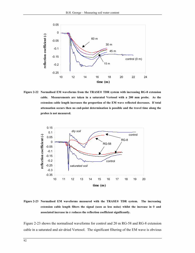
B.H. George – Measuring soil water content
92
-0.25
-0.2
-0.15
-0.1
-0.05
0
0.05
10 12 14 16 18 20 22 24
time (ns)
refle
ctio
n co
effic
ient
(-)
control (0 m)
45 m
15 m
30 m
60 m
Figure 2-22 Normalised EM waveforms from the TRASE® TDR system with increasing RG-8 extension
cable. Measurements are taken in a saturated Vertosol with a 200 mm probe. As the
extension cable length increases the proportion of the EM wave reflected decreases. If total
attenuation occurs then no end-point determination is possible and the travel time along the
probes is not measured.
-0.35-0.3
-0.25-0.2
-0.15-0.1
-0.050
0.050.1
0.15
10 11 12 13 14 15 16 17 18 19 20
time (ns)
refle
ctio
n co
effic
ient
(-)
control
controldry soil
saturated soil
RG-58RG-8
Figure 2-23 Normalised EM waveforms measured with the TRASE® TDR system. The increasing
extension cable length filters the signal (seen as less noise) whilst the increase in θ and
associated increase in σ reduces the reflection coefficient significantly.
Figure 2-23 shows the normalised waveforms for control and 20 m RG-58 and RG-8 extension
cable in a saturated and air-dried Vertosol. The significant filtering of the EM wave is obvious
Chapter 2 – Calibration of TDR and effect of extension cable
93
due to the travel of the EM wave through the extension cables. From the waveforms it is
difficult to visually quantify a difference between the RG-58 and RG-8 cable due to signal loss
leading to a decline in the slope for end-point estimation.
2.5 CONCLUSIONS
Calibration of the TRASE® TDR and Pyelab TDR systems did not yield a significantly
different result to that of the published empirical relationship of Topp et al. (1980). Inclusion
of bulk density (Malicki et al., 1990) in calibration did not significantly improve the
relationship between measured θ and TDR determined √Ka. However, the error in prediction
is larger compared with the results of Topp et al. (1980) and Malicki et al. (1996), and larger
than the standard calibration for the TRASE® TDR system (Skaling, 1992). Large error could
be due to the large clay content and large specific surface of the soil in calibration. Both
TRASE® TDR and Pyelab TDR systems underestimated θ at increased moisture contents, as
others have found (Rothe et al., 1990; Bohl & Roth, 1994). The calibration results are limited
by the uncertainty in determination of ρb when the soil columns were saturated.
Extension cable (RG-58 and RG-8) between the buried probe and the TDR instrument
significantly affects the reported √Ka. However a model accounting for the increasing
extension cable length (RG-58), clay content, soil moisture conditions, TDR system and TDR
probe accounted for only 62.2 % of the variation. Individual estimation of the affect of
extension cable length on reported refractive index shows a linear relationship that is
dependent on the soil type, the TDR instrument and inherent moisture conditions. The
extension cable filters the high frequency EM waves causing a loss in resolution in the
reflected wave by increasing dispersion. I hypothesise that this loss of resolution is shown by a
decrease in the slope of the EM wave used for end-point determination by automatic regimes.
This in turn leads to a subtle, but significant, change in the reported dielectric. The complex
interaction of particle size analysis, specific surface, clay mineralogy and electrical
conductivity on travel of the EM wave is difficult to quantify. When using the TDR technique
for multiple or spatial soil moisture measurements the present recommendation is to
standardise extension cable lengths and calibrate for this extension cable in individual soil
types.
The relationship with cable length is partly determined by the probe type with the SEC probe
and CSIRO probe reacting differently. The CSIRO probe, with the inclusion of a capacitor
assisting generation of the characteristic start point, could be better suited for attenuative

B.H. George – Measuring soil water content
94
(saline) soil. However, the dissipation of energy (of the reflected EM wave) after travelling
through long (> 20 m) extension cables, is a disadvantage of the CSIRO probe.
Chapter 3 - Characteristics of NMM and FD sensors
95
Chapter three
Instrumental characteristics of neutron moderation and
frequency-domain field sensors
3.1. ABSTRACT
The chaotic nature of radioactive decay means the optimum count time for a neutron
moderation probe influences the error of the instrument in measuring soil water content (θ).
For an increasing count time, a CPN Hydroprobe® reported lower variance in a drum of dry
sand and a drum filled with water. The increasing count time however leads to increased time
for measurement in field operation. In field studies using measurements from single tubes, a
32-second count time is recommended. If tubes are to be averaged, or for farmers planning to
schedule irrigation, a 16-second count time is sufficient.
A brief study of the response of the IH1 frequency-domain probe in water and air indicates the
sphere of influence of the IH1 down-hole frequency-domain sensor is limited to 203 mm
radially and approximately 80 mm axially. These results are in accord with previous studies
(Dean et al., 1987) for the IH1 probe and indicate a larger sphere-of-influence than the
EnviroSCAN® (Paltineanu & Starr, 1997).
3.2. NEUTRON MODERATION COUNT RATE AND EFFECT ON ERROR
DETERMINATION AND PRECISION
3.2.1 Introduction
There are many neutron moderation instruments (NMM) commercially available to measure
soil moisture and/or density. This discussion concentrates on NMM meters for determination
of volumetric soil moisture θ (m3 m-3). The precision of a NMM meter in measuring θ
depends on instrument characteristics and the soil that is being measured (van Bavel, 1962;
B.H. George – Measuring soil water content
96
Haverkamp et al., 1984). Early measurements were made with the count times measured in
minutes (van Bavel et al., 1956) and with varying radiation activities and detector methods for
counting the returning thermalised neutrons. More stable electronics and improved count
detectors allow for reduced count times, an important consideration for multiple
measurements. The radiation source strength also affects the required count time to achieve a
nominated precision (Haverkamp et al., 1984; Hodnett & Bell, 1991), however the interaction
between the source and the detector needs to be considered (Haverkamp et al., 1984).
A typical source for modern NMM meters used for θ determination in Australian conditions is
Am-241/Be with a strength of 1.85 GBq (50 mCi). For improved precision, operators can
increase the count time of each measurement (Haverkamp et al., 1984), or take repeated
measurements at shorter count rates (Jayawardane et al., 1983). Here I investigate the effect of
increasing the count time from 1 seconds to 64 seconds on the precision of a NMM in a drum
filled with water and a drum filled with dry sand. This represents the two likely extreme
conditions for the NMM in determination of θ.
3.2.2 Methods and Materials
In two sealed drums measurements at each increasing time interval (1-second (s), 4 s, 16 s, 32
s and 64 s) were taken. The NMM was positioned on a single 50 mm diameter aluminium tube
located axially in the respective 44-gallon (0.20 m3) drum. The source was lowered to 450
mm from the top of the drum and fifty readings taken at each time interval. Readings were
taken with a CPN 503DR Hydroprobe® containing an Am-241/Be (1.85 GBq, 50 mCi) source.
All counts are normalised automatically by the NMM instrument to reflect a 60-second count
scale. Readings were taken between 18 °C and 25 °C ambient air temperature.
One drum contained dry sand, the other water, representing the extreme conditions of
measurement with the NMM instrument. These sealed drums, in conjunction with three other
standards (a drum containing paraffin, one containing a loam soil and one containing
concrete), form the basis of the “universal” calibration used extensively for irrigation
scheduling in Australia. The drum-based calibration is derived from earlier work in cotton-
irrigation scheduling (Cull, 1979).
The water drum, as an infinite source of neutron moderation, is considered as the preferred
standard for normalisation of NMM meters (Hodnett & Bell, 1991). The water drum is used to
calibrate between different meters and to check for instrument drift. Electronic drift is not a
major consideration in modern NMM meters compared to early instruments (Holmes, 1966)

Chapter 3 - Characteristics of NMM and FD sensors
97
and intermittent checks are considered adequate (Williams & Sinclair, 1980; Hodnett & Bell,
1991).
3.2.3 Results and Discussion
Results of the distribution of readings with increasing count time are shown in Figure 3-1. All
count time results are normally distributed (Shapiro & Wilk W test at 5% significance; Steel et
al. 1997) in the sand and water drums. In the water drum, with a count time of 32 s, the data is
normally distributed, however nearly significant (p = 0.061) for non-normal distribution. The
distribution for the 32 s count time shows a slight skew towards larger counts. Testing
between time indicates no difference in the reported mean values (Figure 3-1). Testing
homogeneity of variances indicates a significant difference (corrected χ2 = 1402.28, 196 d.f.; p
< 0.001) using Bartlett’s test (Steel et al., 1997). There is a significant difference between the
count variances with respect to increasing time of count interval. The normal quantile plot,
from readings in the sand drum, is also shown in Figure 3-1 where the shallower the slope
indicates a smaller variance.
250
300
350
400
450
500
550
1 4 16 32 64
time (s) All Pair
s
Tuke
y-Kra
mer 0.
05
.01 .05.10 .25 .50 .75 .90.95 .99
-3 -2 -1 0 1 2 3
normal quantile
1 s
4 s
16 s
32 s 64 s
coun
ts
Figure 3-1 Plot of data in sand drum with increasing count time (seconds) showing (a) spread of data
(variance) decreasing with increasing time count; (b) the Tukey-Kramer test indicating no
significant difference (p = 0.05) between reported means and; (c) the normal quantile plot
(right hand side) showing a decreasing slope with increasing count time indicating a lower
standard deviation.

B.H. George – Measuring soil water content
98
35000
35500
36000
36500
37000
37500
38000
38500
1 4 16 32 64
time (s)
.01 .05.10 .25 .50 .75 .90.95 .99
-3 -2 -1 0 1 2 3
normal quantileAll Pair
s
Tuke
y -Kra
mer 0
.05
coun
ts
1 s
4 s
32 s64 s
16 s
Figure 3-2 Plot of data in water drum with increasing count time (seconds) showing (a) spread of data
(variance) decreasing with increasing time count; (b) the Tukey-Kramer test indicating no
significant difference (p = 0.05) between reported means and; (c) the normal quantile plot
(right hand side) showing a decreasing slope with increasing count time indicating a lower
standard deviation. The rate of decrease in slope is inversely proportional to time.
Results for increasing count time measurements in the water drum are similar to sand (Figure
3-2). Testing homogeneity of variances indicates significant difference between the time
count intervals and their variances (corrected χ2 = 324.48, 196 d.f.; p < 0.001). The normal
quantile plot in the water shows the most dramatic improvement in slope between 1 s and 4 s
count time. As the count time further increases the slope of the normal quantile plot (right-
hand side of Figure 3-2) decreases at a smaller rate.
The count variance shown as standard deviation and standard error of the mean in Table 3-1
decreases as the count time increases. This is expected as the increase in count time part
counters the chaotic (and random) nature of the decay of the Am-241/Be source and Poisson
distribution of the emitted high-energy neutrons. However the increase in measurement time,
whilst reducing variation, obviously increases the total time for measurements with the NMM
in field operations.
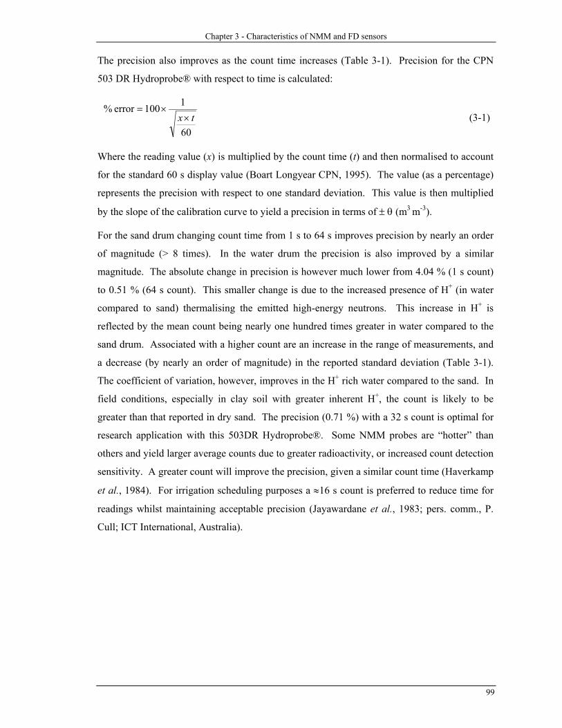
Chapter 3 - Characteristics of NMM and FD sensors
99
The precision also improves as the count time increases (Table 3-1). Precision for the CPN
503 DR Hydroprobe® with respect to time is calculated:
60
1100error %tx×
×= (3-1)
Where the reading value (x) is multiplied by the count time (t) and then normalised to account
for the standard 60 s display value (Boart Longyear CPN, 1995). The value (as a percentage)
represents the precision with respect to one standard deviation. This value is then multiplied
by the slope of the calibration curve to yield a precision in terms of ± θ (m3 m-3).
For the sand drum changing count time from 1 s to 64 s improves precision by nearly an order
of magnitude (> 8 times). In the water drum the precision is also improved by a similar
magnitude. The absolute change in precision is however much lower from 4.04 % (1 s count)
to 0.51 % (64 s count). This smaller change is due to the increased presence of H+ (in water
compared to sand) thermalising the emitted high-energy neutrons. This increase in H+ is
reflected by the mean count being nearly one hundred times greater in water compared to the
sand drum. Associated with a higher count are an increase in the range of measurements, and
a decrease (by nearly an order of magnitude) in the reported standard deviation (Table 3-1).
The coefficient of variation, however, improves in the H+ rich water compared to the sand. In
field conditions, especially in clay soil with greater inherent H+, the count is likely to be
greater than that reported in dry sand. The precision (0.71 %) with a 32 s count is optimal for
research application with this 503DR Hydroprobe®. Some NMM probes are “hotter” than
others and yield larger average counts due to greater radioactivity, or increased count detection
sensitivity. A greater count will improve the precision, given a similar count time (Haverkamp
et al., 1984). For irrigation scheduling purposes a ≈16 s count is preferred to reduce time for
readings whilst maintaining acceptable precision (Jayawardane et al., 1983; pers. comm., P.
Cull; ICT International, Australia).
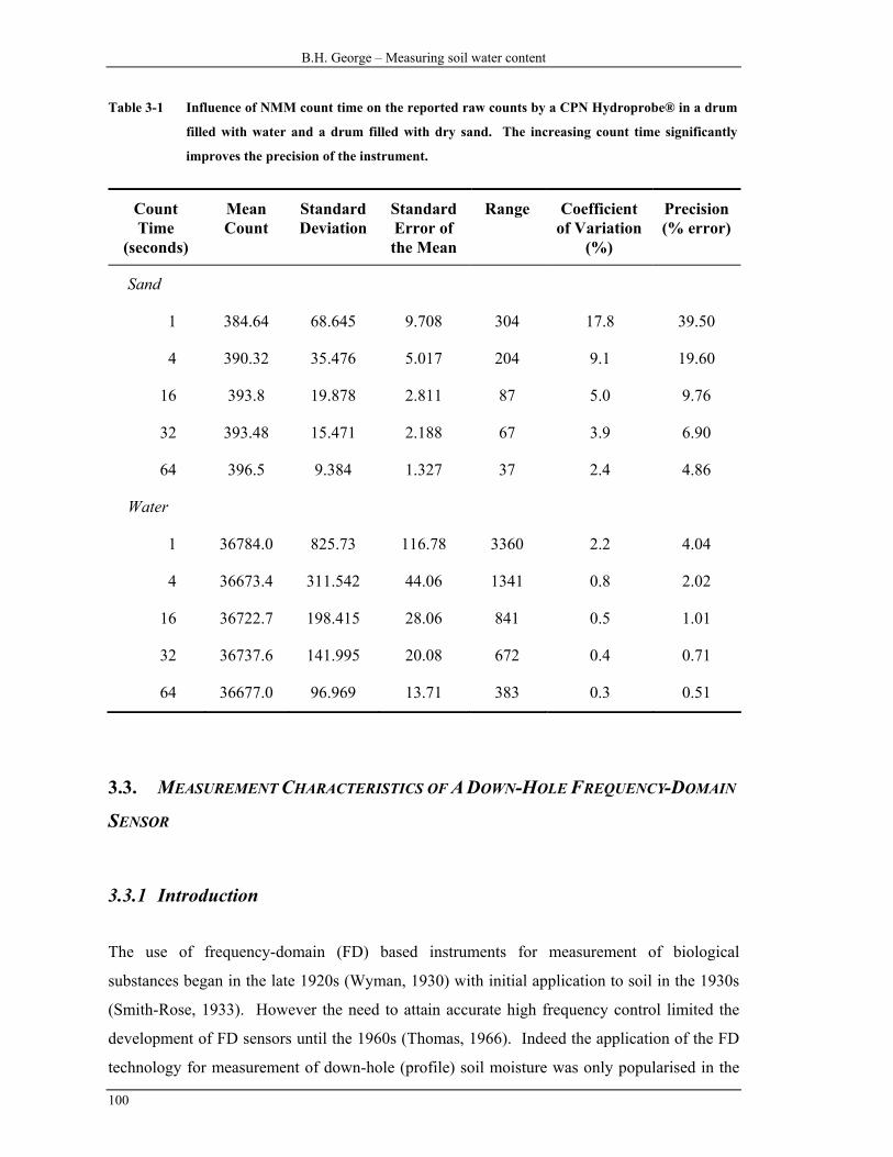
B.H. George – Measuring soil water content
100
Table 3-1 Influence of NMM count time on the reported raw counts by a CPN Hydroprobe® in a drum
filled with water and a drum filled with dry sand. The increasing count time significantly
improves the precision of the instrument.
Count Time
(seconds)
Mean Count
Standard Deviation
Standard Error of the Mean
Range Coefficient of Variation
(%)
Precision (% error)
Sand
1 384.64 68.645 9.708 304 17.8 39.50
4 390.32 35.476 5.017 204 9.1 19.60
16 393.8 19.878 2.811 87 5.0 9.76
32 393.48 15.471 2.188 67 3.9 6.90
64 396.5 9.384 1.327 37 2.4 4.86
Water
1 36784.0 825.73 116.78 3360 2.2 4.04
4 36673.4 311.542 44.06 1341 0.8 2.02
16 36722.7 198.415 28.06 841 0.5 1.01
32 36737.6 141.995 20.08 672 0.4 0.71
64 36677.0 96.969 13.71 383 0.3 0.51
3.3. MEASUREMENT CHARACTERISTICS OF A DOWN-HOLE FREQUENCY-DOMAIN
SENSOR
3.3.1 Introduction
The use of frequency-domain (FD) based instruments for measurement of biological
substances began in the late 1920s (Wyman, 1930) with initial application to soil in the 1930s
(Smith-Rose, 1933). However the need to attain accurate high frequency control limited the
development of FD sensors until the 1960s (Thomas, 1966). Indeed the application of the FD
technology for measurement of down-hole (profile) soil moisture was only popularised in the

Chapter 3 - Characteristics of NMM and FD sensors
101
late 1980s (Dean et al., 1987; Bell et al., 1987). Since then many changes to the circuit
technology and application requirements such as continual measurement systems and portable
sensors, have lead to varied studies of the FD technique (Whalley et al., 1993; Tomer &
Anderson, 1995; Paltineau & Starr, 1997; Wu, 1998).
One question concerning the use of FD technology is the field of influence, or zone of
measurement. The determination of the sphere of influence is in part determined by the sensor
design. This experiment concentrates on the use of down-hole FD probes. The IH1 probe has
a vertical axial sensitivity of 340 mm to 350 mm with 90 % of the influence limited to ± 85
mm from the FD probe centre of sensitivity. Radial sensitivity indicates 90 % of measurement
influence lies within a 130 mm diameter (Dean et al., 1987). The sensitivity of FD probes in
field measurement when compared to neutron moderation method (NMM) is smaller. This is
viewed as an advantage in uniform soil (Ould Mohamed et al., 1997) and a disadvantage in
heterogeneous soil (Evett & Steiner, 1995). This experiment tests the FD probe sensitivity.
Also, I test if there is any effect of rotating the IH1 probe within the access tube during
measurement.
3.3.2 Materials and Methods
In the first experiment readings were taken with a Didcot capacitance soil moisture probe
(Type IH1) inside a 50-mm polyvinyl chloride (PVC) pipe. The readings were taken by
lowering the IH1 probe into the access tube immersed in water. A series of concentric PVC
cylinders of increasing internal diameter (Table 3-2, n = 6) were machined and water was
placed between the IH1 probe and the surrounding PVC at increasing diameters (Figure 3-3).
The IH1 probe has a nominal centre of sensitivity of 114 mm from the bottom of the probe
(Figure 3-4). The frequency was measured in 10 mm increments when the centre of sensitivity
was 20 mm from the water surface to 160 mm from the surface. Six measurements were
recorded at each depth and increasing diameter of the outer tube containing the water. The
readings were taken with the air temperature between 23 °C and 28 °C.

B.H. George – Measuring soil water content
102
AC
EG
I
access tube
water filled bag
305 mm
0 °
90 °270 °
Figure 3-3 Concentric PVC pipes for measurement of the sphere of influence around the Didcot IH1 FD
probe. The PVC access used to lower the FD sensor is centered. The water-filled bag used in
the experiment detecting the sensitivity of the sensor to rotation is shown with the degrees for
rotation from 0° to 345°. To test the volume of influence the outer PVC tubes were filled with
water starting from A (102 mm diameter) and increasing to I (305 mm diameter).
switch
output
centralising rings
centre ofsensitivity
114 mm
Figure 3-4 Dimensions and external components of the Didcot IH1 capacitance probe (Provisional
Manual for the Type IH1 probe, 1992).
In the second experiment a portion of the area between the access tube and the 101.6 mm
diameter PVC pipe was blocked off (approximate cross-sectional area of 2500 mm2) and filled

Chapter 3 - Characteristics of NMM and FD sensors
103
with water (Figure 3-3). The FD technique is more responsive to change in dry soil (Dean et
al., 1987; Kholsa & Persaud, 1997) and the water filled compartment enabled testing of the
probe positioning in the most sensitive frequency range.
The IH1 probe was lowered to 200 mm depth (centre of probe measurement) and a reading
taken. This was performed three times and then the probe rotated 15°. Again the probe was
lowered three times to a depth of 200 mm centre of sensitivity and frequency recorded. The
IH1 probe output is the frequency (Hz) divided by eighty (80). All readings reported here are
the scalar output frequency (true frequency/80).
Table 3-2 PVC pipe dimensions for IH1 FD down-hole probe experiments estimating volume of
influence.
PVC Pipe Internal Diameter (mm)
Average Wall Thickness (mm)
Experimental “run” Number (Figure 3-5)
102 6.4 A
152 7.9 C
203 8.5 E
254 11.0 G
305 11.4 I
3.3.3 Results and Discussion
The reported frequency (f/80 Hz) as the IH1 probe was lowered into the access tube and the
volume of water increased (Table 3-4), is shown in Figure 3-5. Frequency declined as the
probe was lowered into the access tube. An interesting change occurred as the frequency first
stabilised (around 70 mm from the water surface) and then decreased again to a minimum at
140 - 160 mm. The results indicate the majority of the sensitivity (to the water surface) is
within 80 mm of the probe reference point. This is in accord with earlier findings of Dean et
al. (1987) and indicates a larger axial influence than the EnviroSCAN® system studied by
Paltineanu & Starr (1997). The rapid decline between 80 mm and 120 mm below the water
surface, experienced at all diameter increases, is possibly due to the probe design.
Frequency also declined for increasing outer PVC diameters stabilising at 203 mm. Increasing
the diameter of the water filled PVC pipe beyond 203 mm did not significantly (p = 0.05)
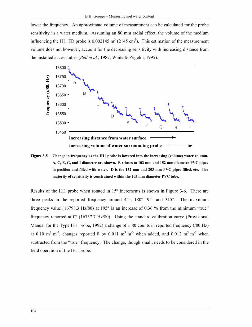
B.H. George – Measuring soil water content
104
lower the frequency. An approximate volume of measurement can be calculated for the probe
sensitivity in a water medium. Assuming an 80 mm radial effect, the volume of the medium
influencing the IH1 FD probe is 0.002145 m3 (2145 cm3). This estimation of the measurement
volume does not however, account for the decreasing sensitivity with increasing distance from
the installed access tubes (Bell et al., 1987; White & Zegelin, 1995).
13450
13500
13550
13600
13650
13700
13750
13800
A
B
C
DE F G H I
freq
uenc
y (f
/80,
Hz)
increasing distance from water surfaceincreasing volume of water surrounding probe
Figure 3-5 Change in frequency as the IH1 probe is lowered into the increasing (volume) water column.
A, C, E, G, and I diameter are shown. B relates to 102 mm and 152 mm diameter PVC pipes
in position and filled with water. D is the 152 mm and 203 mm PVC pipes filled, etc. The
majority of sensitivity is constrained within the 203 mm diameter PVC tube.
Results of the IH1 probe when rotated in 15° increments is shown in Figure 3-6. There are
three peaks in the reported frequency around 45°, 180°-195° and 315°. The maximum
frequency value (16798.3 Hz/80) at 195° is an increase of 0.36 % from the minimum “true”
frequency reported at 0° (16737.7 Hz/80). Using the standard calibration curve (Provisional
Manual for the Type IH1 probe, 1992) a change of ± 80 counts in reported frequency (/80 Hz)
at 0.10 m3 m-3, changes reported θ by 0.011 m3 m-3 when added, and 0.012 m3 m-3 when
subtracted from the “true” frequency. The change, though small, needs to be considered in the
field operation of the IH1 probe.
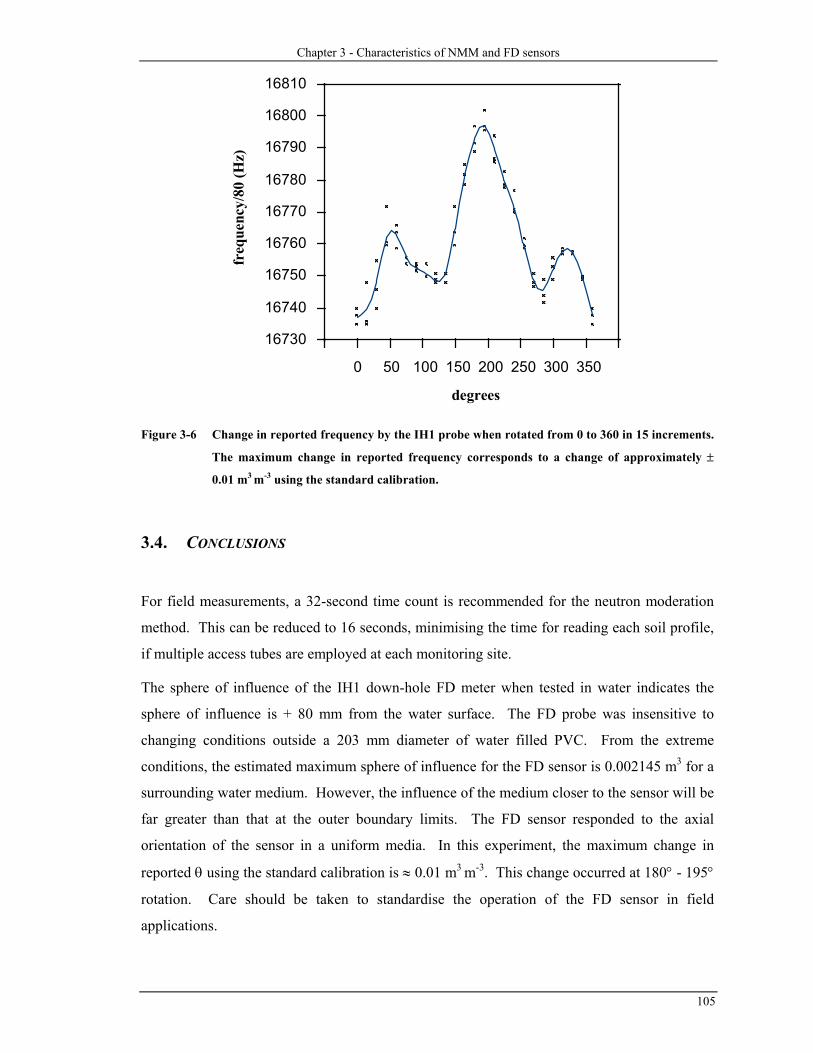
Chapter 3 - Characteristics of NMM and FD sensors
105
16730
16740
16750
16760
16770
16780
16790
16800
16810
0 50 100 150 200 250 300 350
degrees
freq
uenc
y/80
(Hz)
Figure 3-6 Change in reported frequency by the IH1 probe when rotated from 0 to 360 in 15 increments.
The maximum change in reported frequency corresponds to a change of approximately ±
0.01 m3 m-3 using the standard calibration.
3.4. CONCLUSIONS
For field measurements, a 32-second time count is recommended for the neutron moderation
method. This can be reduced to 16 seconds, minimising the time for reading each soil profile,
if multiple access tubes are employed at each monitoring site.
The sphere of influence of the IH1 down-hole FD meter when tested in water indicates the
sphere of influence is + 80 mm from the water surface. The FD probe was insensitive to
changing conditions outside a 203 mm diameter of water filled PVC. From the extreme
conditions, the estimated maximum sphere of influence for the FD sensor is 0.002145 m3 for a
surrounding water medium. However, the influence of the medium closer to the sensor will be
far greater than that at the outer boundary limits. The FD sensor responded to the axial
orientation of the sensor in a uniform media. In this experiment, the maximum change in
reported θ using the standard calibration is ≈ 0.01 m3 m-3. This change occurred at 180° - 195°
rotation. Care should be taken to standardise the operation of the FD sensor in field
applications.

Chapter 4 - Measuring in situ soil water with NMM and dielectric techniques
107
Chapter four
Field measurement of θ with neutron moderation and
dielectric techniques
4.1. ABSTRACT
In situ determination of soil water content (θ) is an important consideration in many soil
studies. For many years the neutron moderation method (NMM) for θ determination down the
soil profile has been carried out. Recently, development in dielectric based techniques for in
situ θ (m3 m-3) measurement has expanded their application and adaptability. However, little
information on how the systems operate in Australian soil conditions is available.
To determine the operational characteristics of the dielectric and NMM techniques, an
experiment in an effluent irrigated Eucalypt plantation was designed. An in situ calibration for
the NMM technique is more sensitive to changing θ than the factory supplied “universal”
calibration. Comparison of the EnviroSCAN® frequency-domain (FD) system and the NMM
count ratio indicates the FD technique is more sensitive to change in θ conditions. The
EnviroSCAN® FD system is well suited to continuous profile-based measurement of θ.
Results with the TDR technique were disappointing, indicating the limited applicability of
TDR in profile based θ measurement in heavy-textured soil, or soil with a large electrical
conductivity. The method of auguring to a known depth and placement of the TDR probe into
undisturbed soil is not recommended.
4.2. INTRODUCTION
Measurement of in situ soil water content (θ) is an important parameter in many soil studies.
The neutron moderation (NMM) technique is widely used and reported for in situ studies (e.g.
Williams et al., 1981; Kamgar et al., 1993). However, little information is available
concerning the use of down-hole frequency-domain (FD) sensors for measurement of θ,

B.H. George – Measuring soil water content
108
especially in Australian conditions. Most field studies of the down-hole FD technique are in
light-textured soil (Tomer & Anderson, 1995; Kholsa & Persaud, 1997; Starr & Paltineanu,
1998). Reports concerning operation of FD sensors in heavy-textured soil are scarce, and poor
precision of a portable down-hole FD system in a fine sandy loam overlaying a sandy clay
loam B horizon soil lead Evett & Steiner (1995) to still favour the NMM technique. However,
the benefits of the FD technology, including the ability to continually measure θ (Paltineanu &
Starr, 1997), being a non-radioactive technology, sensor adaptability (Whalley et al., 1992),
and the improved resolution compared to NMM measurement (Dean et al., 1987), indicate the
potential for the FD technology development. Limiting the FD technology is the need for site
calibration in different soil types (Bell et al., 1987).
The field experiment was designed to investigate the operation of a down-hole FD sensor
(Didcot IH1 probe), a logging FD system (EnviroSCAN®) and a dedicated TDR (TRASE®
TDR). These systems could then be compared with the “standard” NMM (503-DR
Hydroprobe®) technology in an irrigated Eucalypt plantation established in a Brown
Chromosol.
4.3. MATERIALS AND METHODS
4.3.1 The site
The field site is located in the Bunglegumbie Road effluent irrigated plantation on the outskirts
of Dubbo, in NSW (Figure 2-1). The site was developed by the Dubbo City Council for
application of effluent generated in the city. Approximately 20 ha of trees were planted in 1 ha
blocks (Figure 4-1) in 1992. Sensors were located in a block on the northern side of the
plantation in a block of Eucalyptus bicostata spp. bicostata (Victorian Bluegum) shown in
Figure 4-1.
The soil is a Brown Chromosol (Isbell, 1996) typical of the region. The profile description is
detailed in Table 4-1. The applied effluent has not significantly changed the soil chemical or
physical conditions at the site (see Section 3.1 for discussion).

Chapter 4 - Measuring in situ soil water with NMM and dielectric techniques
109
E. grandis
E. grandis
E. grandis
E. grandis
E. grandis
E. grandisC. maculata C. maculata
C. maculata C. maculata
E. bicostata
E. bicostata
E. bicostata
E. cam
aldule
nsis
E. cam
aldule
nsis
E. cam
aldule
nsis
E. cam
aldule
nsis
HybridPoplars
species trial
Willows(salix X)
treatmentworks
Dubbo N
tree
sprinkler
NMM access tubeIH1 FD access tubeEnviroSCAN FD access tubeTDR probes
6 m
4 m
(1) (2) (3)
(4)
(5)
(6)
(7)
(8)
Figure 4-1 Effluent irrigated plantation located on the outskirts of Dubbo. The field site is located in a 1
ha block of E. bicostata trees. The right hand side shows the position of the access tubes and
sensors relative to the E. bicostata trees and sprinklers for irrigation.
4.3.2 Equipment and installation
Neutron moderation (NMM) access tubes were installed in two short transects (Figure 4-1).
Along the first transect, the aluminium access tubes (1.7 m long with a 50 mm outside
diameter) were installed within a 0.5 m radius of three sprinklers. A second transect of NMM
access tubes were installed between the sprinklers (Figure 4-1) approximately 0.7 m apart
normal to the first transect. All NMM readings were taken with a CPN 503DR Hydroprobe®
containing an Am-241/Be (1.85 GBq, 50 mCi) source. Following consideration of the count
time and effect on variance (Section 3.1.3) a 32 second count was used. Readings are
normalised against a water drum count, considered an infinite H+ source (Greacen et al., 1981;
Hodnet & Bell, 1991). Water drum counts were taken approximately weekly during the field
trials with no drift in readings observed.

B.H. George – Measuring soil water content
110
Table 4-1 Profile description at the effluent irrigated plantation.
Horizon Depth (m) Description
A 0 – 0.16 Black to dark reddish brown (5YR 2.5/1 moist, 5YR 3/3 dry);
light sandy clay loam; smooth faced peds; weakly sub-angular
blocky (20 – 50 mm); crumbly; pH = 5.5; even and clear to -
B21 0.16 – 0.50 Very dark brown to dark brown (7.5YR 2.5/3 moist, 7.5YR 3/2);
light medium clay; smooth faced peds; strongly angular blocky
(50 – 100 mm); crumbly, pH = 7.0; irregular and gradual to -
B22 0.5 - Dark reddish brown (5YR 3/3 moist, 5YR 3/2 dry); light clay;
smooth faced peds; strongly angular blocky (50 – 100 mm);
brittle, pH = 6.5
Polyvinyl chloride (PVC) access tubes (1.7 m long with a 50 mm outside diameter) for a
Didcot IH1 FD probe were installed approximately 0.25 m from the NMM access tubes in all
positions (Figure 4-1) following the procedure outlined by Bell et al., 1987. Reported readings
are the average of three (occasionally six) successive readings. During each measurement the
IH1 probe orientation was consistent (setting 0° from East) to reduce bias due to changing
response of the IH1 FD probe to rotation (Figure 3-6). Before and after soil readings the
frequency in air was measured. This is then used with the measured frequency in water to
calculate the universal frequency. For the IH1 down-hole FD probe the universal frequency
(UF) is given by (Didcot Instrument Company, 1992):
)F(F)F(FUF 7.692
water7.692
air
7.692soil
7.692air
−−
= (4-1)
At site (2) and site (3) PVC access tubes were installed for positioning of an EnviroSCAN®
FD system. Though a prototype, the EnviroSCAN® system used was essentially the same in
operation as the system described by Paltineanu & Starr (1997). Fixed sensors were located at
differing depths (Table 4-2) and logged at 20 minute intervals. The software (version 1.1a)
does not allow access to the universal frequency (or scaled frequency) as described by
Paltineanu & Starr (1997). However, a reasonable assumption is that the process to measure
and calculate the UF is the same for prototype EnviroSCAN® used in this experiment. The
UF calibration coefficients for the EnviroSCAN® probe are given in Appendix 4-1.
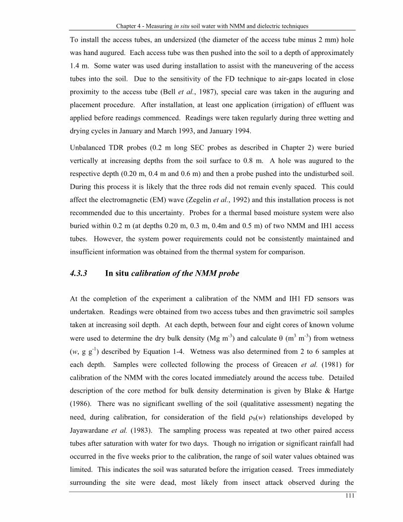
Chapter 4 - Measuring in situ soil water with NMM and dielectric techniques
111
To install the access tubes, an undersized (the diameter of the access tube minus 2 mm) hole
was hand augured. Each access tube was then pushed into the soil to a depth of approximately
1.4 m. Some water was used during installation to assist with the maneuvering of the access
tubes into the soil. Due to the sensitivity of the FD technique to air-gaps located in close
proximity to the access tube (Bell et al., 1987), special care was taken in the auguring and
placement procedure. After installation, at least one application (irrigation) of effluent was
applied before readings commenced. Readings were taken regularly during three wetting and
drying cycles in January and March 1993, and January 1994.
Unbalanced TDR probes (0.2 m long SEC probes as described in Chapter 2) were buried
vertically at increasing depths from the soil surface to 0.8 m. A hole was augured to the
respective depth (0.20 m, 0.4 m and 0.6 m) and then a probe pushed into the undisturbed soil.
During this process it is likely that the three rods did not remain evenly spaced. This could
affect the electromagnetic (EM) wave (Zegelin et al., 1992) and this installation process is not
recommended due to this uncertainty. Probes for a thermal based moisture system were also
buried within 0.2 m (at depths 0.20 m, 0.3 m, 0.4m and 0.5 m) of two NMM and IH1 access
tubes. However, the system power requirements could not be consistently maintained and
insufficient information was obtained from the thermal system for comparison.
4.3.3 In situ calibration of the NMM probe
At the completion of the experiment a calibration of the NMM and IH1 FD sensors was
undertaken. Readings were obtained from two access tubes and then gravimetric soil samples
taken at increasing soil depth. At each depth, between four and eight cores of known volume
were used to determine the dry bulk density (Mg m-3) and calculate θ (m3 m-3) from wetness
(w, g g-1) described by Equation 1-4. Wetness was also determined from 2 to 6 samples at
each depth. Samples were collected following the process of Greacen et al. (1981) for
calibration of the NMM with the cores located immediately around the access tube. Detailed
description of the core method for bulk density determination is given by Blake & Hartge
(1986). There was no significant swelling of the soil (qualitative assessment) negating the
need, during calibration, for consideration of the field ρb(w) relationships developed by
Jayawardane et al. (1983). The sampling process was repeated at two other paired access
tubes after saturation with water for two days. Though no irrigation or significant rainfall had
occurred in the five weeks prior to the calibration, the range of soil water values obtained was
limited. This indicates the soil was saturated before the irrigation ceased. Trees immediately
surrounding the site were dead, most likely from insect attack observed during the

B.H. George – Measuring soil water content
112
measurement period. This significantly limited the transpiration of water from the soil,
leading to wetter than expected conditions.
Calibration of the IH1 FD probe was carried out, however, instrument instability lead to
questioning of the validity of the data and therefore it is not presented here. Others have
experienced similar difficulty in operation of the IH1 FD sensor (pers. comm., P. Lane; Centre
for Forest Tree Technology, Vic). The IH1 FD probe needs to be used with care in field
situations as damage to components is common. In particular, the fibre optic cable is fragile
and prone to catch on branches during measurement. The fibre optic cable links the sensor
output (Figure 3-4) to the readout meter via the inside of the connecting PVC tube. When
operating in the field this cable becomes entangled with leaves or branches and is easily
broken. Also, batteries required by the probe are expensive (≈ $20 each) and last about six
hours. The probe is not designed for continued (rugged) field use.
Table 4-2 Installation depth of sensors in the soil profile.
Depth (m) NMM IH1 EnviroSCAN® TDR
0.10 √ √ √ 0 – 20
0.20 √ √ √ ×
0.30 √ √ √ 0.20 – 0.40
0.40 √ √ √ ×
0.50 √ √ √ 0.40 – 0.60
0.60 √ √ × ×
0.70 × × √ 0.60 – 0.80
0.80 √ √ × ×
0.90 × × √ ×
1.00 √ √ × ×
1.20 √ √ √ ×

Chapter 4 - Measuring in situ soil water with NMM and dielectric techniques
113
4.4. RESULTS AND DISCUSSION
4.4.1 Calibration of the NMM probe
The NMM probe is supplied with a factory based calibration. In Australia, this is based on
calibrations developed by Cull (1979) for a Vertosol in northern NSW. It is accepted that
calibration is required for determination of θ in different soil types (see Section 1.3.3 for
detailed discussion of calibration). The need for calibration in different soil also relates to the
change in bulk density (ρb) down the soil profile (Greacen et al., 1981; Wilson & Ritchie,
1986). The change in ρb and the 95 % confidence interval at the Dubbo site is shown in Figure
4-2. Within sites the ρb is uniform through the soil profile. There is a considerable difference
in the ρb at sites (5) and (6) compared to the larger measured ρb at sites (3) and (7). During site
preparation, for planting of the trees, the soil was ripped to 0.4 m to reduce ρb and improve
root penetration. However, site (3), located near the tree planting line where ripping occurs,
has a significantly larger average ρb than sites (5) and (6). The change in ρb at the four sites is
not readily explained and will affect the calibration process (Fleming et al., 1993). To account
for the change in ρb the count ratio is corrected (with respect to soil dry density) by the
equation of Greacen & Schrale (1976):
nni
b ×=ρρ
' (4-2)
Where n is the count ratio (raw NMM count divided by mean of count in a water drum), bρ is
the mean bulk density for the site, and ρi an individual determination of bulk density at a
particular depth. The factory calibration (Irricrop Technologies Pty. Ltd., NSW Australia) is
based on the work of Cull (1979). This calibration was developed from field studies in a
Vertosol where the ρb down the soil profile remained uniform. The calibration does not
account for different ρb encountered in different soil and within a soil profile. The
methodology for ρb determination used by Cull (1979), with a small surface area and wall
sampling could have influenced his determination of ρb leading to erroneous determination
(Jayawardane et al., 1983).
The combination of information from all horizons will improve the precision of the calibration
(shown by a larger reported r2). However, this procedure introduces an unknown bias into the

B.H. George – Measuring soil water content
114
calibration (Williams & Sinclair, 1981). The introduced experimental bias is minimised by
using a standard technique for tube installation and calibration sampling (Williams and
Sinclair, 1981) and by close location of access tubes relative to each other (Greacen & Hignett,
1979). Instrument bias is more difficult to quantify but should be negligible. A composite
measure of the bias and variance of reported measurement is given by the root mean square
error (RMSE) in the form (Kempthorne & Allmaras, 1986):
variancebiasRMSE 2 += (4-3)
This experiment does not specifically address the issue of bias in reported measurement;
however, minimisation of the RMSE indicates a smaller combined bias and experimental error
(Williams & Sinclair, 1981).
0
0.1
0.2
0.3
0.4
0.5
0.6
0.7
0.8
0.9
1.0 1.2 1.4 1.6 1.8 2.0
site 6site 5
site 7
site 3
ρb (Mg m-3)
dept
h (-
m)
Figure 4-2 Estimation of ρb down the soil profile at four sites during calibration. The 95 % confidence
interval is given. Measurements for ρb were taken at the nominated depth ± 0.03 m.
The estimation of the relationship between the known θ and count ratio (n) for the NMM
across all depths is shown in Figure 4-3a. The estimation is limited by the lack of data at
smaller θ. If several points are removed the fit is significantly improved (Figure 4-3b).
Though corrected for ρb (Equation 4-2) the shaded points represent the smallest ρb at the site.
To reduce the error in establishing the relationship these points are excluded from the
prediction curve (Figure 4-4) with a decreased RMSE (0.029 from Figure 4-3b). Even so, the
error in prediction is still large, and the calibration should be considered with care. Clearly,

Chapter 4 - Measuring in situ soil water with NMM and dielectric techniques
115
more data, especially at smaller θ, is required before confidence in this calibration is
reasonable (< 0.03 m3 m-3 95 % confidence).
0.3
0.4
0.5
0.6
0.7
0.8
0.9
0.20 0.30 0.40 0.50θ (known)
ρ b cor
rect
ed N
MM
cou
nt r
atio
n’ = 0.147 +1.142 × θr2 = 0.55
0.3
0.4
0.5
0.6
0.7
0.8
0.9
0.20 0.30 0.40 0.50
ρ b cor
rect
ed N
MM
cou
nt r
atio
θ (known)
n’ = 0.099 + 1.171 × θr2 = 0.91
Figure 4-3 (a) Estimation of the relationship between the corrected count ratio (n’), accounting for ρb,
and known θ (RMSE = 0.071). (b) Estimation of the relationship between the corrected count
ratio (n’) and known θ, with points excluded (shown) where ρb correction did not improve the
relationship (RMSE = 0.029).
0.15
0.20
0.25
0.30
0.35
0.40
0.45
0.50
0.55
0.60
0.35 0.40 0.45 0.50 0.55 0.60 0.65 0.70 0.75
NMM count ratio (n’)
θ (m
3 m-3
)
θ = -0.0842 + 0.85412×n’
Figure 4-4 Calibration for the NMM probe at the Dubbo site. To predict θ from the adjusted n (for ρb)
the relationship is given by: θ = -0.0842 + 0.85412 × n’. The 95 % confidence interval (CI) is
shown indicating large error (≈ 0.05 m3 m-3) associated with this calibration.
Calibration of the NMM for prediction of θ is shown in Figure 4-4. The error estimate in
prediction, the 95 % confidence interval, is based on Equation 2-8 (Webster, 1997). There is

B.H. George – Measuring soil water content
116
significant error in determination of the known θ for calibration. To improve this calibration,
further sampling at smaller moisture contents is required.
4.4.2 Comparison with the factory supplied “universal” calibration
The relationship between the calibration for the NMM in the Brown Chromosol to the factory
supplied “universal” calibration is shown in Figure 4-5a. The effect of ρb is encompassed in
the “universal” calibration and different depths are readily identified. The modeled effect of ρb
on the “universal” calibration is then compared to the site calibration (Figure 4-5b). There is
still an identified difference when ρb < 1.5 Mg m-3. This is possibly due to the prediction of
the “universal calibration” not accurately estimating the effect of ρb, or the inability of the ρb
normalisation of Greacen & Shrale (1976) to account for changing ρb at the Dubbo site.
0.3
0.4
0.5
0.3 0.4 0.5 0.6
θ (in situ calibration)
θ (“
univ
ersa
l” c
alib
ratio
n)
0.2 m
0.4 m
0.3
0.4
0.5
0.3 0.4 0.5 0.6
BD < 1.5θ = 0.035 + 0.773 θin situ,
r2 = 0.973
BD > 1.5θ = 0.046 + 0.825 θin situ,
r2 = 0.988
θ (in situ calibration)
θ (“
univ
ersa
l” c
alib
ratio
n)
Figure 4-5 (a) Plot of θ reported by the factory supplied “universal calibration” and the in situ site
calibration. The different calibrations (from Appendix 4-2) are readily identified. (b)
Relationship between the modeled “universal calibration” and the site based calibration
accounting for the site ρb at different depths in the four measured profiles.
The site calibration reports a greater θ compared to the “universal” calibration, particularly
when the soil is wet. Given the large error in the site calibration (≈ 0.05 m3 m-3, 95 % CI),
there is no significant difference between the reported θ from the site calibration and the
“universal” equation at depths < 0.6 m when the soil profile dries (Figure 4-6).
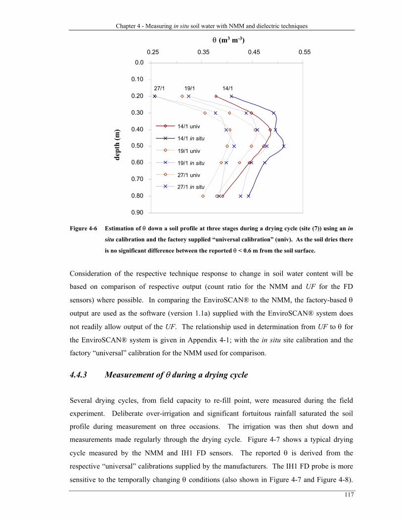
Chapter 4 - Measuring in situ soil water with NMM and dielectric techniques
117
0.0
0.10
0.20
0.30
0.40
0.50
0.60
0.70
0.80
0.90
0.25 0.35 0.45 0.55
θ (m3 m-3)
dept
h (m
) 14/1 univ
14/1 in situ
19/1 univ
19/1 in situ
27/1 univ
27/1 in situ
14/119/127/1
Figure 4-6 Estimation of θ down a soil profile at three stages during a drying cycle (site (7)) using an in
situ calibration and the factory supplied “universal calibration” (univ). As the soil dries there
is no significant difference between the reported θ < 0.6 m from the soil surface.
Consideration of the respective technique response to change in soil water content will be
based on comparison of respective output (count ratio for the NMM and UF for the FD
sensors) where possible. In comparing the EnviroSCAN® to the NMM, the factory-based θ
output are used as the software (version 1.1a) supplied with the EnviroSCAN® system does
not readily allow output of the UF. The relationship used in determination from UF to θ for
the EnviroSCAN® system is given in Appendix 4-1; with the in situ site calibration and the
factory “universal” calibration for the NMM used for comparison.
4.4.3 Measurement of θ during a drying cycle
Several drying cycles, from field capacity to re-fill point, were measured during the field
experiment. Deliberate over-irrigation and significant fortuitous rainfall saturated the soil
profile during measurement on three occasions. The irrigation was then shut down and
measurements made regularly through the drying cycle. Figure 4-7 shows a typical drying
cycle measured by the NMM and IH1 FD sensors. The reported θ is derived from the
respective “universal” calibrations supplied by the manufacturers. The IH1 FD probe is more
sensitive to the temporally changing θ conditions (also shown in Figure 4-7 and Figure 4-8).

B.H. George – Measuring soil water content
118
For all field measurements two times the standard deviation (for 95 % of this time) of the
measured frequency was < 6 counts (Hz/80) giving a confidence interval of 0.01 – 0.03 m3 m-3
depending on θ. This repeatability is typical of the FD technique (Bell et al., 1987).
0.0
0.10
0.20
0.30
0.40
0.50
0.60
0.70
0.80
0.90
0.25 0.30 0.35 0.40 0.45 0.50 0.55
θ (m3 m-3)
dept
h (m
)
14/1
19/1
27/1
17/1
22/125/1
(a)
0.0
0.2
0.4
0.6
0.8
1.0
1.2
0.0 0.10 0.20 0.30 0.40 0.50 0.60
θ (m3 m-3)
dept
h (m
)14/117/120/123/125/127/129/12/3
14/12/3(b)
Figure 4-7 Drying cycle measured with the NMM at site (7) using the in situ calibration (a) and by the
IH1 FD probe (b).
The IH1 FD probe is more sensitive to change in the θ when the factory “universal” calibration
is used. The relationship between reported θ by the NMM (“universal” and in situ calibration)
and IH1 FD probe (“universal” calibration) is shown in Figure 4-8. The increased range
(between the two respective readings) indicates the FD probe is more sensitive to the change in
θ compared to the NMM. The IH1 FD probe reports smaller θ than the NMM instrument as
the profile dries. This could be due to the sensitivity of the technique (Dean et al., 1987) or an
effect of the calibration procedure.

Chapter 4 - Measuring in situ soil water with NMM and dielectric techniques
119
0.0
0.20
0.40
0.60
0.80
1.00
1.20
1.40
0 0.1 0.2 0.3 0.4 0.5
θ (m3 m-3)
dept
h (m
)
NMM univNMM in situ FD
27/1 14/1
Figure 4-8 Determination of θ by the FD and NMM instruments with factory “universal” calibration
and in situ calibration for the NMM instrument. The IH1 FD sensor is more sensitive to the
change in θ conditions compared to the NMM technique shown by the large range of
reported θ during the drying cycle.
4.4.4 Calibration and operational considerations of the IH1 probe
The NMM calibration almost exclusively indicates a linear response to increasing θ in soil
conditions (e.g. Holmes, 1966; Cull, 1979; Greacen & Hignett, 1979; Jayawardane et al.,
1983; O’Leary & Incerti, 1993). The response of the IH1 FD probe to θ is soil dependent
(Bell et al., 1987). Initial field calibration indicated a linear relationship for small variations in
θ, and, when considering the measured frequency, this could be incorporated into a general
calibration (Bell et al., 1987). The IH1 FD probe is supplied with a factory calibration based
on a power function shown in Equation 4-4. The equation (4-4) is sensitive to change in θ
condition especially when the soil is wet.
( )( )UF12.731 21.50 ××= UFIHθ (4-4)
As the measured frequency in soil approaches the water based frequency the determination of
θ increases dramatically. Smaller frequency readings leading to a UF > 1 (from Equation 4-1)
are not reported in the literature. However, soil with significant electrical conductivity can
B.H. George – Measuring soil water content
120
cause a decline in the measured frequency, leading to overestimation of the UF and therefore
overestimation of θ. A response to increasing salinity can be estimated by Equation 4-5
modeling the complex impedance of a capacitor (C) in parallel with a conductance (G).
For the IH1 down-hole FD probe, C is the capacitance of the soil-electrode (assembly) in a
non-conductive soil. In a conductive soil let Ceff be the effective capacitance. Noting the
angular frequency of oscillation (ϖ) is constant for the IH1 probe (7 × 10⁸ s-1). When the
electrodes are placed in the soil, the G/C ratio is equal to specific conductance of the soil. For
small values of G, C is not changed significantly (the multiplier in the bracket ≈ 1). However,
as the conductance increases, the effective C increases leading to a smaller measured
frequency. This can lead to a UF > 1 and overestimation of θ (pers. comm., J.D. Cooper;
Institute of Hydrology, UK).
4
22
2
1
+=
CGCCeff ϖ
(4-5)
In determining the UF, the water used in calculation of Fwater should be indicative of the likely
soil electrical conductivity conditions. During this experiment calculation of the UF was
undertaken with available tap water and this introduced a small but unmeasured error into the
UF determination.
Another non-linear relationship (for the FD technique) developed from measurement in a silt
loam soil (Paltineanu & Starr, 1997) uses a power function:
1674.2& 490.0 UFSP ×=θ (4-6)
This equation is more sensitive at small soil water contents (θ), becoming less sensitive as the
θ increases and is related to Equation 4-4 by:
1& log0829.054707.0 IHSP θθ ×+= (4-7)
Where θP&S is the θ from Equation 4-6, and θIH1 is the θ in Equation 4-4. If we assume the
NMM responds linearly to increasing θ we can plot the UF against the count ratio (n) to see
how the IH1 FD sensor responds to increasing θ (shown by increasing n). Figure 4-9 shows
all data of the IH1 down-hole FD probe plotted against the corresponding NMM count ratio.
There is no readily identified relationship and an investigation of specific depths (Figure 4-10)
shows little relationship between the measured UF and the measured n. The linear fit, at each
depth, is shown for reference. Transformation of data (including log and reciprocal of both
axis) and different fit techniques (including spline and polynomial fit) did not significantly

Chapter 4 - Measuring in situ soil water with NMM and dielectric techniques
121
reduce the RMSE in fit. The IH1 FD probe is sensitive to change in θ conditions, however this
change cannot be readily related to the NMM technique. Also, heterogeneity in θ condition
immediately surrounding the IH1 FD probe could lead to reporting of different θ conditions.
Clearly further study is required to gain confidence in the field use of the IH1 probe for
reporting θ.
0.80
0.85
0.90
0.95
1.00
0.40 0.45 0.50 0.55 0.60 0.65 0.70 0.75
NMM count ratio (-)
UF
(-)
Figure 4-9 Plot of all UF data (combined sites and depths) against the NMM count ratio (n) at the
Dubbo site. There is no readily identified relationship between the data indicating a different
response to θ conditions.
0.80
0.85
0.90
0.95
1.00
0.40 0.50 0.60 0.70NMM count ratio (-)
UF
(-)
r2 = 0.48d = 0.2 m
0.80
0.85
0.90
0.95
1.00
0.40 0.50 0.60 0.70NMM count ratio (-)
UF
(-)
r2 = 0.50d = 0.3 m
0.80
0.85
0.90
0.95
1.00
0.40 0.50 0.60 0.70NMM count ratio (-)
UF
(-)
r2 = 0.32d = 0.4 m
0.80
0.85
0.90
0.95
1.00
0.40 0.50 0.60 0.70NMM count ratio (-)
UF
(-)
r2 = 0.32d = 0.5 m
0.80
0.85
0.90
0.95
1.00
0.40 0.50 0.60 0.70NMM count ratio (-)
UF
(-)
r2 = 0.28d = 0.6 m
0.80
0.85
0.90
0.95
1.00
0.40 0.50 0.60 0.70
NMM count ratio (-)
UF
(-)
r2 = 0.20d = 0.8 m
0.80
0.85
0.90
0.95
1.00
0.40 0.50 0.60 0.70
NMM count ratio (-)
UF
(-)
r2 = 0.005d = 1.0 m
0.80
0.85
0.90
0.95
1.00
0.40 0.50 0.60 0.70
NMM count ratio (-)
UF
(-)
r2 = 0.05d = 1.2 m
Figure 4-10 Depth plots of UF measured by the IH1 FD probe and the NMM count ratio (n). The linear
fit is shown.
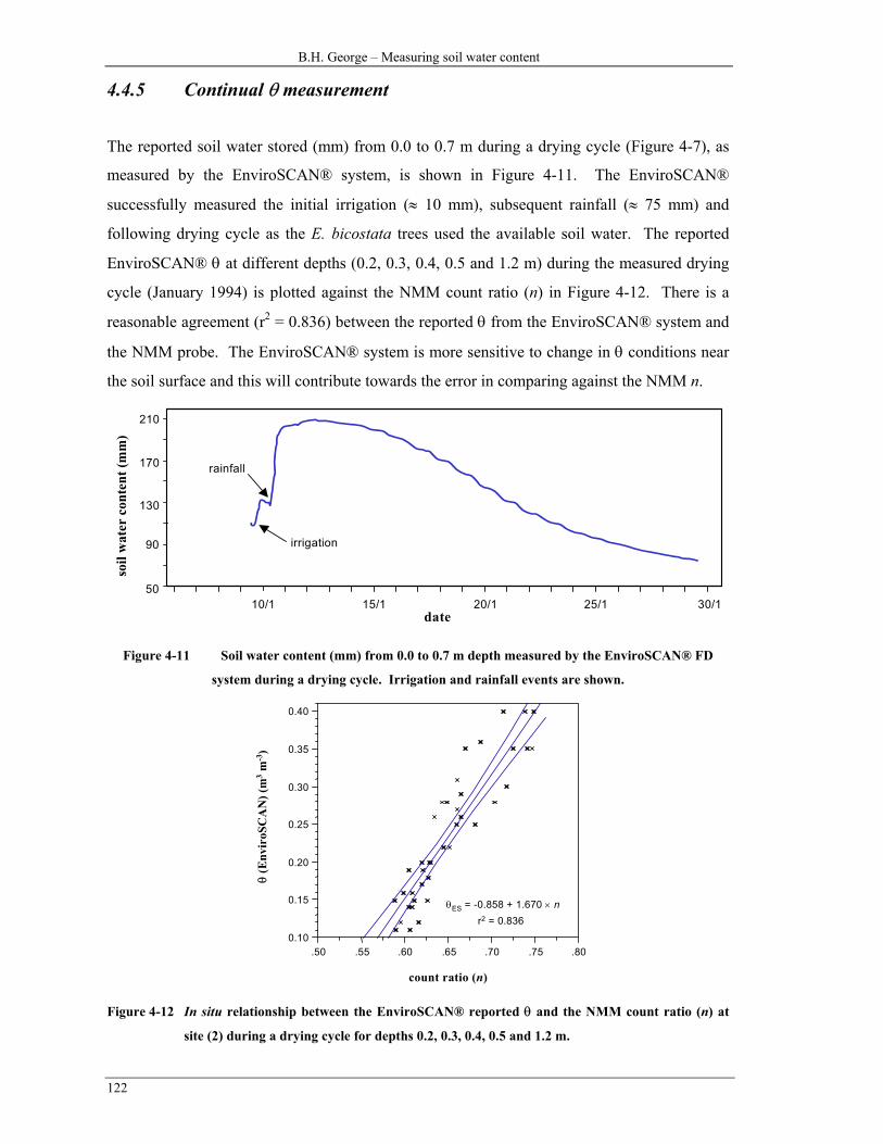
B.H. George – Measuring soil water content
122
4.4.5 Continual θ measurement
The reported soil water stored (mm) from 0.0 to 0.7 m during a drying cycle (Figure 4-7), as
measured by the EnviroSCAN® system, is shown in Figure 4-11. The EnviroSCAN®
successfully measured the initial irrigation (≈ 10 mm), subsequent rainfall (≈ 75 mm) and
following drying cycle as the E. bicostata trees used the available soil water. The reported
EnviroSCAN® θ at different depths (0.2, 0.3, 0.4, 0.5 and 1.2 m) during the measured drying
cycle (January 1994) is plotted against the NMM count ratio (n) in Figure 4-12. There is a
reasonable agreement (r2 = 0.836) between the reported θ from the EnviroSCAN® system and
the NMM probe. The EnviroSCAN® system is more sensitive to change in θ conditions near
the soil surface and this will contribute towards the error in comparing against the NMM n.
10/1 15/1 20/1 25/1 30/1date
soil
wat
er c
onte
nt (m
m)
50
90
170
210
130
irrigation
rainfall
Figure 4-11 Soil water content (mm) from 0.0 to 0.7 m depth measured by the EnviroSCAN® FD
system during a drying cycle. Irrigation and rainfall events are shown.
0.10
0.15
0.20
0.25
0.30
0.35
0.40
.50 .55 .60 .65 .70 .75 .80
count ratio (n)
θ (E
nvir
oSC
AN
) (m
3 m-3
)
θES = -0.858 + 1.670 × nr2 = 0.836
Figure 4-12 In situ relationship between the EnviroSCAN® reported θ and the NMM count ratio (n) at
site (2) during a drying cycle for depths 0.2, 0.3, 0.4, 0.5 and 1.2 m.

Chapter 4 - Measuring in situ soil water with NMM and dielectric techniques
123
0
40
50
20
10
30
Jan Feb Mar AprMonth
Soil
wat
er c
onte
nt (m
m)
Figure 4-13 Continual measurement of θ at 0.1 m depth with the EnviroSCAN® system in 1993. The
continual monitoring shows the effect of the short irrigation system used for effluent
application in February.
A major advantage of the EnviroSCAN® system is the ability to continually obtain data.
Figure 4-14 shows the changing soil water conditions with continued irrigation during late
summer and autumn in 1993. Concentrating on the period between March 17 and April 10, θ
at 0.10 m varies with the small irrigation amounts applied (nominally 5 mm daily). In this
system the small increase in reported θ at 1.20 m depth around March 25 indicates the soil
profile at that time was saturated with water moving beyond the sensor depth.
0
40
50
20
10
30
Soil
wat
er c
onte
nt (m
m)
60
15/3 20/3 25/3 1/4 5/5 10/515/4 20/4 25/410/45/4 30/4
Date
1.2 m
0.1 m
Figure 4-14 Continual measurement of θ at 0.1 m and 1.2 m depth with the EnviroSCAN® system in
1993.
4.4.6 Measurement with time-domain reflectometry (TDR)
Temporal measurement of θ down the TDR profile (Table 4-2) was not successful at site (2) or
site (3) where TDR probes were installed (Figure 4-1). Probes continually failed, especially at
large θ. Associated with the large reported θ was an increasing error (Figure 4-15), notably
B.H. George – Measuring soil water content
124
deeper in the soil profile. Attenuation of the generated electromagnetic (EM) waveform
caused most failure. Figure 4-16 shows the attenuation of the EM wave during measurement.
The inability to obtain the end-point reflection was consistent at both sites and all depths,
except 0 – 0.2 m, at varying times. One possible reason for the ability to continually monitor θ
in the 0 – 0.2 m depth is the lighter textured soil due to the A horizon. As the clay content
increases with depth it is possible that the electrical conductivity also increases leading to
attenuation of the EM wave, especially in wet conditions. The electrical conductivity hindered
the use of TDR probes > 0.2 m in a Vertosol because of the EM attenuation (Bridge et al.,
1996). Also, at the Dubbo field site, the installation of the TDR probes was sub-optimal.
Some converging (unmeasured) of the three prong unbalanced probes could potentially have
lead to changing the properties of the EM wave travelling through the soil. The ability of the
TDR instrument to obtain and interpret a significant reflection is dependent on the power of
the generated EM wave (pers. comm., H. Fancher; Soilmoisture Equipment Corp., CA USA),
the interaction of the probe spacing (Zegelin et al., 1989), and soil properties such as bulk
electrical conductivity (Dalton, 1992).
Attenuation of the EM waveform is a significant problem in Australian soil where increased
clay contents and inherent salt leads to increasing electrical conductivity. This is a particular
problem when the soil is wet. There are several options to improve the ability of the TDR
technique in saline environments including: an increase in the power generation of the EM
wave; reduction of the length of the probes embedded in the soil (the EM wave then has less
opportunity for attenuation); or coating the probes with a small dielectric material (Knight et
al., 1997). During calibration measurements with a 0.15 m unbalanced probe, at depths
greater than 0.15 m, could not be obtained (graph not shown) indicating that the problem is
significant in Brown Chromosols and probably other soil with a large clay content.
Attenuation in saturated Vertosols can limit the (TRASE®) TDR to 0.15 m probes in the top
soil (data not shown). If the bulk soil electrical conductivity is measured the maximum probe
length can be estimated using the procedure outlined by Dalton (1992). By reducing the
maximum operating length of the probes the reported TDR results become more susceptible to
local variation in θ and the interpretation of the EM waveforms by automated analysis more
difficult (Young et al., 1997).

Chapter 4 - Measuring in situ soil water with NMM and dielectric techniques
125
0.00.100.200.300.400.500.600.700.800.901.00
1/7 1/9 1/11
1/13
1/15
1/17
1/19
1/21
1/23
1/25
date
θ (m
3 m-3
)
00.20.40.6
95 % CI
rain
fall
+irr
igat
ion
Figure 4-15 Measuring θ during a drying cycle with TDR probes buried at 0 – 0.2 m, 0.2 - 0.4 m, 0.4 – 0.6
m and 0.6 – 0.8 m own a soil profile. Error shown is the 95 % confidence interval for
measured θ. Readings on 1-Jan and 13-Jan are slightly offset for interpretation of associated
error.
0
500
1000
1500
2000
2500
3000
0 200 400 600 800 1000 1200 1400
time (ns)
rela
tive
volta
ge o
utpu
t
Figure 4-16 Attenuation of the EM waveform due to increased electrical conductivity leading to an
inability to detect the EM reflection from the end of the probes in the soil.
B.H. George – Measuring soil water content
126
4.5. CONCLUSIONS
An in situ calibration of an NMM probe in a Brown Chromosol suggests the “universal
calibration” underestimates θ at large water contents. The calibration was carried out in a
limited θ range and the associated error limits the application of the in situ calibration. Error
was reduced by the application of a bulk density correction function (Greacen & Shrale, 1976).
However, at smaller bulk density ( ρb < 1.4), the correction function was not as effective.
The determination of the frequency of FD probes in water (Fwater) as part of the UF should be
considered in more detail. Results here indicate that the determination of UF in available tap
water may lead to an overestimation of the UF in saline soil conditions. The FD technology is
more sensitive to change in θ, especially when compared to the NMM technique. This
improved resolution allows detection of small changes in θ but could be a disadvantage in
heterogeneous soil.
A good relationship between the EnviroSCAN® system and the measured NMM count ratio
(n) indicates the two systems both respond to changing θ conditions. The ability of the
EnviroSCAN® system to continually monitor θ is a considerable advantage over other labour
intensive systems.
The TDR technique was unable to measure θ when the soil was wet, especially at depths > 0.2
m. This was due to the attenuation of the EM wave along the 0.2 m unbalanced probes and
this is likely to limit the application of the TDR technique for profile based measurement.

Chapter 5 - Measuring water content in iron ore
127
Chapter five
Measuring moisture content of stockpiled iron ore with the
Time-Domain Reflectometry technique
5.1. ABSTRACT
Moisture content is important in determining the handling characteristics of processed iron ore.
When moisture content is too high (> 0.1 g g-1) handling is difficult and causes excess wear on
machinery. If the stockpiled ore moisture can be measured, transport at optimum moisture
contents may be undertaken. Time-domain reflectometry is a technique suited to in situ
measurement of moisture in porous media. However, iron (Fe) present in soil is known to
affect the dielectric properties. Recent studies suggest that large concentrations of Fe are likely
to limit the ability of TDR in moisture determination (Robinson et al., 1994). The
electromagnetic waveforms require careful analysis to ensure accurate measurement of the
actual travel time along the embedded probes in the iron ore. Calibration of TDR for
determination of moisture content is recommended.
I calibrated the TDR method to measure moisture in a processed iron ore. The polynomial
relationship between the refractive index (√Ka) measured by the TDR technique and known
moisture (m3 m-3), aa KK ×−×+−= 034.0410.0776.0θ , is particularly sensitive at higher
moisture contents.
I then conducted a field trial to measure the change in moisture over time of iron ore layered in
a stockpile. In the field study, a linear relationship between refractive index and moisture
exists. This relationship, 0.053)( 0.0770.0725)197.0( ±−×−= mKaθ (m3 m-3), is not
significantly different from the laboratory polynomial fit when constrained to similar moisture
contents.
The 28 m extension cable used to connect the probes to the TDR affected the end-point
determination of the TDR system. To account for this, 0.197 should be subtracted from
reported Ka before calculation of volumetric moisture content. Protection of the extension

B.H. George – Measuring soil water content
128
cable from the buried probe to the measurement node is necessary to stop the shear force of the
ore stretching and snapping the cable. This is overcome by placing the extension cable inside a
common garden hose and looping the hose near the probe insertion place in the stockpile.
5.2. INTRODUCTION
Time-domain reflectometry (TDR) is widely utilised in the study of saturated and unsaturated
water determination and movement in soil. The technique, being based on the media dielectric
surrounding the probes, can be influenced by the magnetic properties. However, in
determination of volumetric moisture content (θ, m3 m-3) in porous media, the effect of
inherent magnetic properties (H, tesla; see Mullins, 1977 for discussion of appropriate units) is
neglected as the electromagnetic (EM) wave travels in transverse mode (see Equation 1-12 and
Equation 1-21). One element that has magnetic properties is iron (Fe). Iron is generally found
in some soil in the form of goethite, haematite, ferrihydrite, maghemite and to a lesser extent
(the primary mineral) magnetite. Robinson et al. (1994) found that very high concentrations of
Fe present in the soil significantly affected the θ reported by the TDR technique. However, in
most soil-based situations, this effect is unlikely to be a major influence on reported θ. The
changing response of the TDR technique in determining the apparent dielectric (Ka) is an
opportunity to exploit the TDR technique if a reasonable calibration is developed.
The mining and processing of iron ore is a major enterprise in the Australian economy.
Ranked fourth in the world, Australia is a major producer and exporter of iron ore
(http://www.minerals.org.au/facts/iron.htm). The ore is mined and then processed for bulk
transfer, generally by train and/or ship, for further processing. The moisture content of iron ore
(during processing and in stockpiles) is an important consideration of post-processing handling
characteristics (Harbert et al., 1974). During the refining process water is added. If the
moisture content of the ore is too large then handling is difficult (Guerra, 1974). The main
concern is freighting the iron ore to the port facility by train, and the “dumping” process where
the ore is removed from train to conveyors for loading onto ore carriers (ships). Further
problems can arise in maintaining processed ore within contract specifications for total
moisture content (pers. comm. W. Thomas; Advanced Technical Development, Technical
Resources Pty. Ltd., Australia).
On-line measurement of iron ore is not routinely carried out though Yip & Cutmore (1993)
have successfully investigated continued measurement of free and bound water in iron ore
during process transport. Bound water in this context relates to water retained by the iron ore

Chapter 5 - Measuring water content in iron ore
129
after drying at 378 °K (Yip & Cutmore, 1993). There are different techniques available for
moisture content determination including infra-red reflectance (Harbert et al., 1974) and
neutron moderation and attenuation (Cutmore et al., 1996). Non-invasive on-line measurement
is carried out by microwave attenuation at high frequencies between 2 to 4 GHz. However
attenuation of the generated EM wave restricts the penetration of the wave into the ore sample.
Cutmore et al. (1996) suggest a maximum penetration of 150 mm at 10 % moisture by weight
(w = 0.1 g g-1). The TDR technique can partially overcome this uncertainty by utilisation of
probes to guide the travel of the EM wave through the iron ore. Also the ability to connect
probes to extension cable allows for measurement of θ within formed stockpiles. Our aim is to
measure θ in stockpiles. To achieve this we first need to establish the relationship between the
refractive index (√Ka) of the ore material and θ in controlled conditions. From this
understanding we can then adapt the TDR technique for field based measurement of iron ore.
5.3. LABORATORY CALIBRATION
5.3.1 Materials and Methods
Processed iron ore from the Mt Tom Price mine (22° 40’ 00”, 117° 46’ 00”; Western
Australia), shown in Figure 5-1, was sieved to remove the > 5 mm diameter fraction. The
cumulative ore characteristics are shown in Table 5-1. Haematite is the dominant form of iron
present in the high-grade processed ore. The ore was dried (378 °K for 24 hours) and packed
into a 0.25 m × 0.25 m × 0.20 m plastic container. 11.701 kg of ore was placed into the
container filling a volume of 4.05 l. Thus the ore was packed to a (natural) density of 2.89 Mg
m-3. An unbalanced three-wire TDR probe (200 mm long) was placed into the middle of the
container after half the ore was poured in. The rest of the ore was poured over the probe
ensuring good contact with the stainless steel rods. Possible end effects were minimised by
ensuring at least 20 mm between the end of the probe and the side of the container.
All readings were taken with the ore temperature between 18 °C – 19 °C (291 °K – 293 °K).
Six readings of the Ka were recorded with a TRASE® TDR system (Soilmoisture Equipment
Corporation, Santa Barbara, CA, USA) with one reading stored as a graph. The container was
then emptied and repacked twice more to obtain further readings. This process was then
repeated with a different TDR probe. For each known moisture content the associated TDR
reading consisted of triplicate packing of the container and six measurements made each time
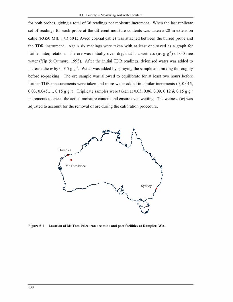
B.H. George – Measuring soil water content
130
for both probes, giving a total of 36 readings per moisture increment. When the last replicate
set of readings for each probe at the different moisture contents was taken a 28 m extension
cable (RG50 MIL 17D 50 Ω Avico coaxial cable) was attached between the buried probe and
the TDR instrument. Again six readings were taken with at least one saved as a graph for
further interpretation. The ore was initially oven dry, that is a wetness (w, g g-1) of 0.0 free
water (Yip & Cutmore, 1993). After the initial TDR readings, deionised water was added to
increase the w by 0.015 g g-1. Water was added by spraying the sample and mixing thoroughly
before re-packing. The ore sample was allowed to equilibrate for at least two hours before
further TDR measurements were taken and more water added in similar increments (0, 0.015,
0.03, 0.045,…, 0.15 g g-1). Triplicate samples were taken at 0.03, 0.06, 0.09, 0.12 & 0.15 g g-1
increments to check the actual moisture content and ensure even wetting. The wetness (w) was
adjusted to account for the removal of ore during the calibration procedure.
Mt Tom Price
Sydney
Dampier
Figure 5-1 Location of Mt Tom Price iron ore mine and port facilities at Dampier, WA.
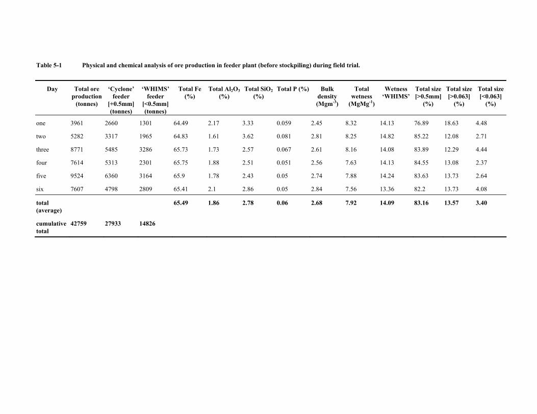
Table 5-1 Physical and chemical analysis of ore production in feeder plant (before stockpiling) during field trial.
Day Total ore production
(tonnes)
‘Cyclone’ feeder
[+0.5mm] (tonnes)
‘WHIMS’ feeder
[<0.5mm] (tonnes)
Total Fe (%)
Total Al2O3(%)
Total SiO2 (%)
Total P (%) Bulk density (Mgm-3)
Total wetness
(MgMg-1)
Wetness ‘WHIMS’
Total size [>0.5mm]
(%)
Total size [>0.063]
(%)
Total size [<0.063]
(%)
one 3961 2660 1301 64.49 2.17 3.33 0.059 2.45 8.32 14.13 76.89 18.63 4.48
two 5282 3317 1965 64.83 1.61 3.62 0.081 2.81 8.25 14.82 85.22 12.08 2.71
three 8771 5485 3286 65.73 1.73 2.57 0.067 2.61 8.16 14.08 83.89 12.29 4.44
four 7614 5313 2301 65.75 1.88 2.51 0.051 2.56 7.63 14.13 84.55 13.08 2.37
five 9524 6360 3164 65.9 1.78 2.43 0.05 2.74 7.88 14.24 83.63 13.73 2.64
six 7607 4798 2809 65.41 2.1 2.86 0.05 2.84 7.56 13.36 82.2 13.73 4.08
total (average)
65.49 1.86 2.78 0.06 2.68 7.92 14.09 83.16 13.57 3.40
cumulative total
42759 27933 14826

B.H. George – Measuring soil water content
132
5.3.2 Results and Discussion
5.3.2.1 Calibration of TDR for estimation of iron ore moisture content
The spray wetting procedure produced an even wetting in the iron ore sample used in
calibration with a low reported standard error in the sampled ore at five increasing w values
(Table 5-2). The removal of ore to estimate w required a small change in the calculation of
actual w. This corrected w value is used in all further calculations.
The first check of w (0.03 g g-1) reported close to the correct wetness. As moisture content
increased a maximum difference of 0.0131 g g-1 between actual (average) w and measured w
occurred at a target moisture content of 0.15 g g-1. During the wetting up process segregation
of finer material into clumps was observed and this could account for the differences in total
average w and measured w from three samples. The deviation of measured w (n = 3) did not
increase at higher moisture contents.
Table 5-2 Actual w for calibration with TRASE® TDR and associated check values.
Target w (g g-1) Actual w (g g-1) Measured w
(g g-1)
Standard
Deviation
(± g g-1)
Actual –
Measured
0.00 0.00 -- -- --
0.015 0.0150 -- -- --
0.030 0.0299 0.0295 0.00036 0.0005
0.045 0.0454 -- -- --
0.060 0.0609 0.0569 0.0013 -0.0040
0.070 0.0768 -- -- --
0.090 0.0928 0.0879 0.0012 0.0049
0.105 0.1091 -- -- --
0.120 0.1255 0.1158 0.00096 0.0097
0.135 0.1423 -- -- --
0.150 0.1593 0.1462 0.00089 0.0131
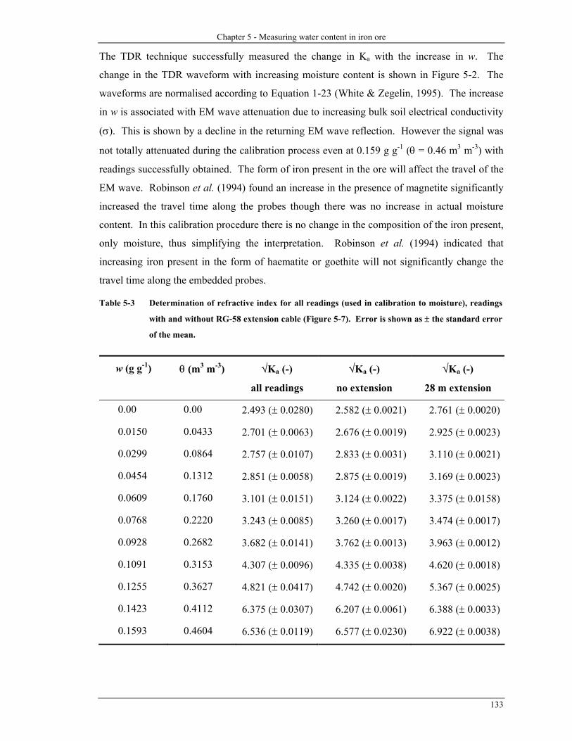
Chapter 5 - Measuring water content in iron ore
133
The TDR technique successfully measured the change in Ka with the increase in w. The
change in the TDR waveform with increasing moisture content is shown in Figure 5-2. The
waveforms are normalised according to Equation 1-23 (White & Zegelin, 1995). The increase
in w is associated with EM wave attenuation due to increasing bulk soil electrical conductivity
(σ). This is shown by a decline in the returning EM wave reflection. However the signal was
not totally attenuated during the calibration process even at 0.159 g g-1 (θ = 0.46 m3 m-3) with
readings successfully obtained. The form of iron present in the ore will affect the travel of the
EM wave. Robinson et al. (1994) found an increase in the presence of magnetite significantly
increased the travel time along the probes though there was no increase in actual moisture
content. In this calibration procedure there is no change in the composition of the iron present,
only moisture, thus simplifying the interpretation. Robinson et al. (1994) indicated that
increasing iron present in the form of haematite or goethite will not significantly change the
travel time along the embedded probes.
Table 5-3 Determination of refractive index for all readings (used in calibration to moisture), readings
with and without RG-58 extension cable (Figure 5-7). Error is shown as ± the standard error
of the mean.
w (g g-1) θ (m3 m-3) √Ka (-)
all readings
√Ka (-)
no extension
√Ka (-)
28 m extension
0.00 0.00 2.493 (± 0.0280) 2.582 (± 0.0021) 2.761 (± 0.0020)
0.0150 0.0433 2.701 (± 0.0063) 2.676 (± 0.0019) 2.925 (± 0.0023)
0.0299 0.0864 2.757 (± 0.0107) 2.833 (± 0.0031) 3.110 (± 0.0021)
0.0454 0.1312 2.851 (± 0.0058) 2.875 (± 0.0019) 3.169 (± 0.0023)
0.0609 0.1760 3.101 (± 0.0151) 3.124 (± 0.0022) 3.375 (± 0.0158)
0.0768 0.2220 3.243 (± 0.0085) 3.260 (± 0.0017) 3.474 (± 0.0017)
0.0928 0.2682 3.682 (± 0.0141) 3.762 (± 0.0013) 3.963 (± 0.0012)
0.1091 0.3153 4.307 (± 0.0096) 4.335 (± 0.0038) 4.620 (± 0.0018)
0.1255 0.3627 4.821 (± 0.0417) 4.742 (± 0.0020) 5.367 (± 0.0025)
0.1423 0.4112 6.375 (± 0.0307) 6.207 (± 0.0061) 6.388 (± 0.0033)
0.1593 0.4604 6.536 (± 0.0119) 6.577 (± 0.0230) 6.922 (± 0.0038)
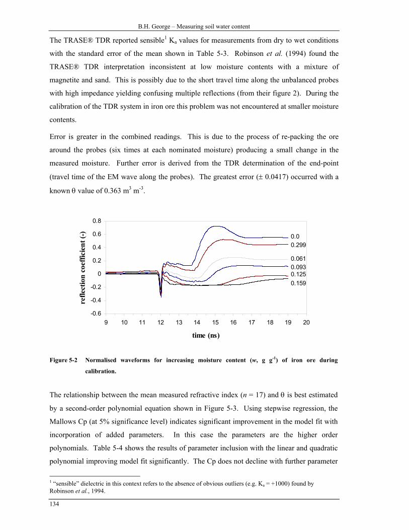
B.H. George – Measuring soil water content
134
The TRASE® TDR reported sensible1 Ka values for measurements from dry to wet conditions
with the standard error of the mean shown in Table 5-3. Robinson et al. (1994) found the
TRASE® TDR interpretation inconsistent at low moisture contents with a mixture of
magnetite and sand. This is possibly due to the short travel time along the unbalanced probes
with high impedance yielding confusing multiple reflections (from their figure 2). During the
calibration of the TDR system in iron ore this problem was not encountered at smaller moisture
contents.
Error is greater in the combined readings. This is due to the process of re-packing the ore
around the probes (six times at each nominated moisture) producing a small change in the
measured moisture. Further error is derived from the TDR determination of the end-point
(travel time of the EM wave along the probes). The greatest error (± 0.0417) occurred with a
known θ value of 0.363 m3 m-3.
-0.6
-0.4
-0.2
0
0.2
0.4
0.6
0.8
9 10 11 12 13 14 15 16 17 18 19 20
time (ns)
refle
ctio
n co
effic
ient
(-)
0.00.299
0.0610.0930.1250.159
Figure 5-2 Normalised waveforms for increasing moisture content (w, g g-1) of iron ore during
calibration.
The relationship between the mean measured refractive index (n = 17) and θ is best estimated
by a second-order polynomial equation shown in Figure 5-3. Using stepwise regression, the
Mallows Cp (at 5% significance level) indicates significant improvement in the model fit with
incorporation of added parameters. In this case the parameters are the higher order
polynomials. Table 5-4 shows the results of parameter inclusion with the linear and quadratic
polynomial improving model fit significantly. The Cp does not decline with further parameter
1 “sensible” dielectric in this context refers to the absence of obvious outliers (e.g. Ka = +1000) found by Robinson et al., 1994.
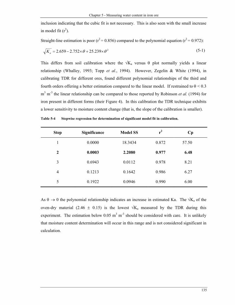
Chapter 5 - Measuring water content in iron ore
135
inclusion indicating that the cubic fit is not necessary. This is also seen with the small increase
in model fit (r2).
Straight-line estimation is poor (r2 = 0.856) compared to the polynomial equation (r2 = 0.972):
2239.25752.2659.2 θθ ×+×−=aK (5-1)
This differs from soil calibration where the √Ka versus θ plot normally yields a linear
relationship (Whalley, 1993; Topp et al., 1994). However, Zegelin & White (1994), in
calibrating TDR for different ores, found different polynomial relationships of the third and
fourth orders offering a better estimation compared to the linear model. If restrained to θ < 0.3
m3 m-3 the linear relationship can be compared to those reported by Robinson et al. (1994) for
iron present in different forms (their Figure 4). In this calibration the TDR technique exhibits
a lower sensitivity to moisture content change (that is, the slope of the calibration is smaller).
Table 5-4 Stepwise regression for determination of significant model fit in calibration.
Step Significance Model SS r2 Cp
1 0.0000 18.3434 0.872 57.50
2 0.0003 2.2080 0.977 6.48
3 0.6943 0.0112 0.978 8.21
4 0.1213 0.1642 0.986 6.27
5 0.1922 0.0946 0.990 6.00
As θ → 0 the polynomial relationship indicates an increase in estimated Ka. The √Ka of the
oven-dry material (2.46 ± 0.15) is the lowest √Ka measured by the TDR during this
experiment. The estimation below 0.05 m3 m-3 should be considered with care. It is unlikely
that moisture content determination will occur in this range and is not considered significant in
calculation.

B.H. George – Measuring soil water content
136
0.0
1.0
2.0
3.0
4.0
5.0
6.0
7.0
8.0
0.0 0.1 0.2 0.3 0.4 0.5
θ (m3 m-3)
√Ka
(-)
√Ka = 2.648 - 2.101×θ + 23.947×θ2
r2 = 0.977
Figure 5-3 Polynomial relationship between the √Ka (-) and the known volumetric moisture content, θ
(m3 m-3), for processed iron ore from Mt. Tom Price mine. The highest standard error of the
mean (±0.05) occurred when known θ was 0.39 m3 m-3. The 95% confidence interval for the
equation fit is shown.
In order to exploit a relationship between the measured √Ka and θ the inverse estimation
technique (Webster, 1997) is employed. Thus, inverting equation 5-1 the estimation of θ from
measured √Ka for the iron ore is given by the equation:
aa KK ×−×+−= 034.0410.0776.0θ (5-2)
and shown in Figure 5-4 with associated error in prediction.
-0.1
0
0.1
0.2
0.3
0.4
0.5
0.6
2.0 3.0 4.0 5.0 6.0 7.0
measured √Ka (-)
θ (m
3 m-3
)
error in predicted fit
error in individualprediction
Figure 5-4 Calibration of TDR for determination of θ in iron ore from measured √Ka. Confidence limits
are 95% for prediction of line and individual points respectively (SAS, 1995).

Chapter 5 - Measuring water content in iron ore
137
5.3.2.2 Effect of transmission cable on reported √Ka
In field based measurements an RG-58 transmission cable (28 m length) was utilised to
connect the buried probe to the measuring TDR instrument. The extension cable influences
the travel of the EM wave (Chapter 2). Normalised waveforms (Equation 1-23) at 0.0, 0.061
and 0.126 g g-1 are shown in Figure 5-5. The EM waveform is filtered, as it travels through the
cable, and then into the lossy media (iron ore). Qualitatively this is observed with a loss of
resolution in resulting waveform. For all moisture contents the transmission cable caused a
loss of signal. The information loss can also lead to a small change in the start and end-point
determination of the EM wave. Most TDR systems employ an automatic end-point
determination analysis. These systems will preferably err in a systematic form with the change
in end-point determination then quantified.
The relationship of measured √Ka and the influence of the extension cable is shown in Figure
5-6. The linear fit (r2 = 0.991) of the plotted mean (n = 5 - 10) measurements shows that the
addition of extension cable between the TDR instrument and the probe increases the reported
√Ka. The modeled increase:
extension)(no 0211.11966.0)(extension aa KK ×+= (5-3)
requires further consideration in field based estimation of iron ore θ by the TDR technique.
Though statistically significant (p = 0.05, paired t-test output for slope, data not shown)
indicating a difference from a slope equal to one, the relationship between Ka with extension
cable and without extension cable is essentially 1:1.
The statistical difference is due to the low error associated between reading with, and without,
extension cable. Therefore in order to account for the effect of the extension cable on the EM
wave in determining true √Ka, 0.197 should be subtracted from the measured √Ka before
predicting θ when this RG-58 cable is used.

B.H. George – Measuring soil water content
138
-0.6
-0.4
-0.2
0
0.2
0.4
0.6
0.8
0 2 4 6 8 10 12
time (ns)
refle
ctio
n co
effic
ient
(-)
w = 0.0 θ = 0.0
extension
(a)
-0.4
-0.3
-0.2
-0.1
0
0.1
0.2
0.3
0 2 4 6 8 10 12
time (ns)
refle
ctio
n co
effic
ient
(-)
w = 0.061 θ = 0.176
extension
(b)
-0.3
-0.25
-0.2
-0.15
-0.1
-0.05
0
0.05
0 2 4 6 8 10 12
time (ns)
refle
ctio
n co
effic
ient
(-)
w = 0.126 θ = 0.363
extension
(c)
Figure 5-5 Effect of a 28 m RG-58 transmission cable on reflection coefficient for increasing moisture
content in iron ore: (a) 0.0 g g-1; (b) 0.061 g g-1; (c) 0.126 g g-1.
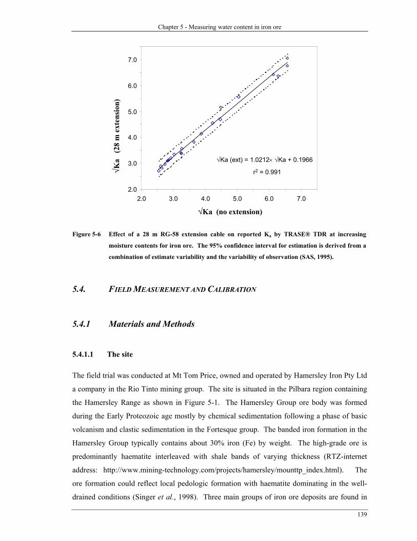
Chapter 5 - Measuring water content in iron ore
139
2.0
3.0
4.0
5.0
6.0
7.0
2.0 3.0 4.0 5.0 6.0 7.0
√Ka (no extension)
√Ka
(28
m e
xten
sion
)
√Ka (ext) = 1.0212× √Ka + 0.1966
r2 = 0.991
Figure 5-6 Effect of a 28 m RG-58 extension cable on reported Ka by TRASE® TDR at increasing
moisture contents for iron ore. The 95% confidence interval for estimation is derived from a
combination of estimate variability and the variability of observation (SAS, 1995).
5.4. FIELD MEASUREMENT AND CALIBRATION
5.4.1 Materials and Methods
5.4.1.1 The site
The field trial was conducted at Mt Tom Price, owned and operated by Hamersley Iron Pty Ltd
a company in the Rio Tinto mining group. The site is situated in the Pilbara region containing
the Hamersley Range as shown in Figure 5-1. The Hamersley Group ore body was formed
during the Early Proteozoic age mostly by chemical sedimentation following a phase of basic
volcanism and clastic sedimentation in the Fortesque group. The banded iron formation in the
Hamersley Group typically contains about 30% iron (Fe) by weight. The high-grade ore is
predominantly haematite interleaved with shale bands of varying thickness (RTZ-internet
address: http://www.mining-technology.com/projects/hamersley/mounttp_index.html). The
ore formation could reflect local pedologic formation with haematite dominating in the well-
drained conditions (Singer et al., 1998). Three main groups of iron ore deposits are found in

B.H. George – Measuring soil water content
140
the local region. At the Mt Tom price mine the most common ore is from the Brockman Iron
Formation. This ore, further defined by composition of elements, is considered a “premium
lump” with low phosphate (< 0.05 %) and high Fe (> 64 %) contents (http://www.mining-
technology.com/projects/hamersley/ mounttp_index.html).
The mining operation commenced in 1966 and extends 7.5 km over six principal locations in
the ore body. The mining procedures aim to separate the high grade from the lower grade ore.
The lower grade ore is fed to the concentrator plant where ore is physically treated to produce
three fractions:
• oversize (> 30mm)
• lump product (6 mm < lump < 30 mm)
• fines product (< 6 mm)
The oversize fraction is returned through the processing plant to produce either lump product
or fines. The fines fraction is then stockpiled for blending with other quality product in
shipments to the port facility (based at Dampier, WA). The fines generally end processing
with a (gravimetric) moisture content between 10 – 14 % (w = 0.10 – 0.14 g g-1). Due to the
high moisture content the fines are termed “wet fines”. For handling and shipping purposes an
optimum w of 0.08 g g-1 is preferred (pers. comm. N. Poetschka; Hamersley Iron Pty Ltd.,
Australia). To achieve this the wet fines ore is stockpiled for several days before
transportation to the port facilities. The WHIMS plant is the final processing stage where the
wet fines are produced before stockpiling.
The stockpiles are created by a ‘stacker’ that normally produces a stockpile of dimensions 18.5
m high, 53 m wide, approximately 375 m long with an internal wall angle of 35o (pers. comm.
W. Thomas, Advanced Technical Development, Australia). This process requires
approximately 160 passes of the stacker, normally taking about five days, with the ore layered
in a chevron pattern. After a period of draining the wet fines are reclaimed and loaded into
train cars for shipment to the port facility.
5.4.1.2 Experimental design
The original design placed thirty horizontally buried TDR probes (supplied by CSIRO; Glen
Osmond, SA) in the stockpile in three locations, points (A), (B) and (C) in Figure 5-7. The
probes were to be stratified to assist in determining the intra-stockpile variability. Production
problems in the WHIMS section of the ore processing forced a change in the stockpile design
and location of TDR probes. The final dimensions of the stockpile are shown in Figure 5-7.

Chapter 5 - Measuring water content in iron ore
141
At cross section A, the final height of the stockpile was 9.35 m. For cross sections B and C the
heights were 11.11 m and 14.75 m respectively.
stockpile base (m)
heig
h t (m
)
0 20 40 60 80 1000
4
8
12
16A B C
(20)
Figure 5-7. Schematic side view of actual stockpile of wet fines ore with cross sections where TDR probes
were positioned. At the completion of the experiment density and calibration samples were
taken from these cross-sections.
The stockpile was built over a period of six days by the stacker moving along the length of the
stockpile dropping the ore from varying height (typically 1.5 ± 0.5 m) above the pile. As the
stacker passed a position in the pile the probes were buried in the recently layed ore. The
probes were covered with ore (using a hand shovel) and once the stacker had returned to cover
the position again a measurement was taken with the probe connected directly to the TRASE®
TDR (Soilmoisture Equipment Corporation, Santa Barbara, CA, USA). A 28 m extension
cable (RG-58 coaxial cable) was connected to the probe and buried at 300 mm depth along the
side of the stockpile leading to a common point for the cross section (A, B and C respectively).
Initial readings with the TDR instrument were satisfactory. Some probes (e.g. C01) failed
when further ore stacked on top of the building stockpile cause mass movement down the edge
of the stockpile shearing the extension cable. This problem was overcome by threading the
extension cable through common garden hose before burying the probe and extension cable in
the stockpile. The extension cable, now housed in the garden hose, was collected in two loops
(approximately 2m of cable) at the base of the buried probe. This technique was utilised to
account for shift of the TDR probe as the layered ore above was stacked. Probe locations are
shown in Figure 5-8. Five probes failed at some stage during the ore stacking processes.
Notably none of the probes protected with the common garden hose failed.

B.H. George – Measuring soil water content
142
The calibration of the TRASE® TDR required determination of bulk density (ρb). Two
techniques were tested in ρb determination. The core method (Blake & Hartge, 1986) is
commonly used in calibration for TDR measurements in porous material. To obtain
measurements steel cylinders (51.2 mm internal diameter, 200 mm length) were hammered in
around the buried probe. The wet and dry ρb was then determined after weighing and drying.
A second technique, the sand replacement method (Blake & Hartge, 1986), was also used.
This is the more common method for mining engineers in this situation. A small hole
(approximately 300 mm deep and a radius of 200 mm) is dug in the iron ore and a known mass
of sand then replaces the iron ore. The mass and volume are then used to calculate the ρb as
described by Blake & Hartge (1986).
Permeability was determined at all cross-sections during reclamation (unpublished data,
P.Lam, MPA Williams & Associates, Australia). Values for cross section C are included in
Appendix 5-1. Personal observations indicated lower permeability occurred where finer
material congregated on falling from the stacker. This was not quantitatively assessed.
Generally the ore is considered free draining.
5.4.2 Results and Discussion
After insertion and connection to an extension cable, triplicate readings on all probes were
taken at approximately six-hour intervals. A field calibration was established accounting for
changes in ρb. The field calibration also tested the laboratory calibration in situ. Further,
probes were measured with a TRASE® TDR immediately after installation before extension
cable was attached and then immediately after the extension cable was connected. This
accounted for the influence of cable extension on the reported Ka and is discussed in further
detail. The determination of ρb was attempted with two techniques and a consideration of the
limitation in measurement with the standard core method (Section 1.2.4.1) in comparison to
the more robust sand-replacement technique is discussed.

Chapter 5 - Measuring water content in iron ore
143
(20) (10) 0 10 200
5
10
15
20
A3
A2
A1
heig
ht (m
)
stockpile base (m)
reclaimer side stacker side
(20) (10) 0 10 200
5
10
15
20
B1 B1 B3 B4
B7B6B5
heig
ht (m
)
stockpile base (m)
reclaimer side stacker side
(20) (10) 0 10 200
5
10
15
20
C19
C16
C14 C08
C01 C02 C03 C04 C05 C06
C15 C09
C12 C18
C17
B1
B2
B3
B5
C11
C10
B4
heig
ht (m
)
stockpile base (m)
reclaimer side stacker side
Figure 5-8 TDR probe locations at three cross-sections of stockpile. Due to production problems ore was
directed over cross-section C to achieve regular stockpile height and formation.

B.H. George – Measuring soil water content
144
5.4.2.1 Calibration to θ
To obtain an estimation of the ore θ, a field calibration of the TDR technique is required.
Calibration of the TDR measured Ka against the calculated θ is shown in Figure 5-9 with the
refractive index (√Ka) plotted against the calculated moisture content of the ore. Testing the
linear relationships (Mead et al., 1993) indicates no significant difference between field and
laboratory calibrations (p = 0.05) with F2,22 degrees of freedom. Similar results were obtained
with a t-test procedure for determination of slope difference outlined by Steel & Torrie (1980).
In comparison, data from the laboratory calibration below 0.15 m3 m-3 were excluded and a
linear model fitted. The two linear calibrations are shown in Figure 5-9. The slopes are almost
identical with the significant difference in the intercept. For a measured θ the predicted √Ka is
higher (+0.634) in the field calibration. This calibration is used for conversion to θ for the
field trial results.
One possible explanation for the increase in intercept for field calibration is the changing ρb
conditions. ρb was estimated around the probe locations during the reclamation of the ore
stockpile (for transport). Across the stockpile mean dry ρb was 2.66 (± 0.18) Mg m-3 from 41
sand replacement measurements. The mean was used where ρb determination was not made
within 2 m of the TDR probe. The determination of ρb is discussed further in Section 5.4.2.3.
1.5
2.5
3.5
4.5
5.5
6.5
7.5
0.1 0.15 0.2 0.25 0.3 0.35 0.4 0.45 0.5
θ 3 m (m -3)
√Ka
(-)
(field) √Ka = 1.458 + 12.128× θ
(r2 = 0.880)
(laboratory) √Ka = 0.824 + 12.068× θ(r2 = 0.928)
laboratory
Figure 5-9 Calibration of in situ iron ore moisture content from refractive index measured by TDR.
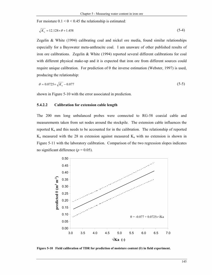
Chapter 5 - Measuring water content in iron ore
145
For moisture 0.1 < θ < 0.45 the relationship is estimated:
458.1128.12 +×= θaK (5-4)
Zegelin & White (1994) calibrating coal and nickel ore media, found similar relationships
especially for a Bayswater meta-anthracite coal. I am unaware of other published results of
iron ore calibrations. Zegelin & White (1994) reported several different calibrations for coal
with different physical make-up and it is expected that iron ore from different sources could
require unique calibration. For prediction of θ the inverse estimation (Webster, 1997) is used,
producing the relationship:
077.00725.0 −×= aKθ (5-5)
shown in Figure 5-10 with the error associated in prediction.
5.4.2.2 Calibration for extension cable length
The 200 mm long unbalanced probes were connected to RG-58 coaxial cable and
measurements taken from set nodes around the stockpile. The extension cable influences the
reported Ka and this needs to be accounted for in the calibration. The relationship of reported
Ka measured with the 28 m extension against measured Ka with no extension is shown in
Figure 5-11 with the laboratory calibration. Comparison of the two regression slopes indicates
no significant difference (p = 0.05).
0.00
0.05
0.10
0.15
0.20
0.25
0.30
0.35
0.40
0.45
0.50
3.0 3.5 4.0 4.5 5.0 5.5 6.0 6.5 7.0
√Ka (-)
pred
icte
d θ
(m3 m
-3)
θ = -0.077 + 0.0725×√Ka
Figure 5-10 Field calibration of TDR for prediction of moisture content (θ) in field experiment.
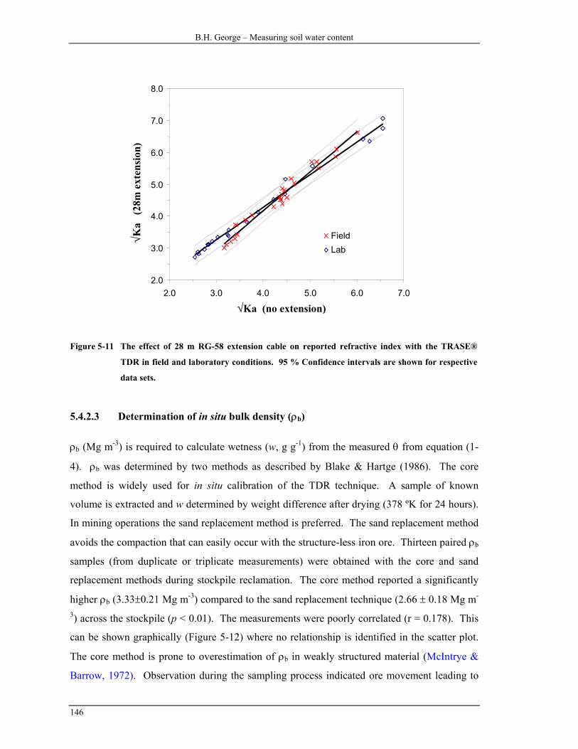
B.H. George – Measuring soil water content
146
2.0
3.0
4.0
5.0
6.0
7.0
8.0
2.0 3.0 4.0 5.0 6.0 7.0
√Ka (no extension)
√Ka
(28
m e
xten
sion
)
FieldLab
Figure 5-11 The effect of 28 m RG-58 extension cable on reported refractive index with the TRASE®
TDR in field and laboratory conditions. 95 % Confidence intervals are shown for respective
data sets.
5.4.2.3 Determination of in situ bulk density (ρb)
ρb (Mg m-3) is required to calculate wetness (w, g g-1) from the measured θ from equation (1-
4). ρb was determined by two methods as described by Blake & Hartge (1986). The core
method is widely used for in situ calibration of the TDR technique. A sample of known
volume is extracted and w determined by weight difference after drying (378 ºK for 24 hours).
In mining operations the sand replacement method is preferred. The sand replacement method
avoids the compaction that can easily occur with the structure-less iron ore. Thirteen paired ρb
samples (from duplicate or triplicate measurements) were obtained with the core and sand
replacement methods during stockpile reclamation. The core method reported a significantly
higher ρb (3.33±0.21 Mg m-3) compared to the sand replacement technique (2.66 ± 0.18 Mg m-
3) across the stockpile (p < 0.01). The measurements were poorly correlated (r = 0.178). This
can be shown graphically (Figure 5-12) where no relationship is identified in the scatter plot.
The core method is prone to overestimation of ρb in weakly structured material (McIntrye &
Barrow, 1972). Observation during the sampling process indicated ore movement leading to
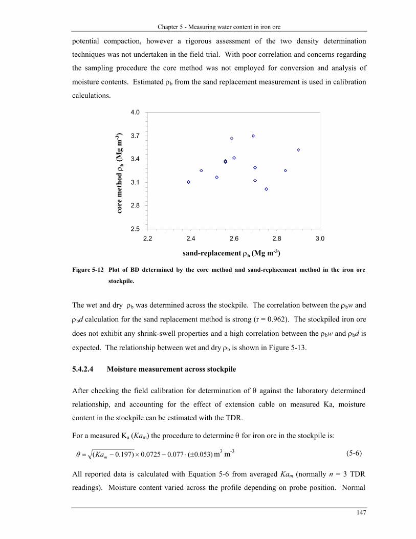
Chapter 5 - Measuring water content in iron ore
147
potential compaction, however a rigorous assessment of the two density determination
techniques was not undertaken in the field trial. With poor correlation and concerns regarding
the sampling procedure the core method was not employed for conversion and analysis of
moisture contents. Estimated ρb from the sand replacement measurement is used in calibration
calculations.
2.5
2.8
3.1
3.4
3.7
4.0
2.2 2.4 2.6 2.8 3.0
sand-replacement ρb (Mg m-3)
core
met
hod
ρ b (M
g m
-3)
Figure 5-12 Plot of BD determined by the core method and sand-replacement method in the iron ore
stockpile.
The wet and dry ρb was determined across the stockpile. The correlation between the ρbw and
ρbd calculation for the sand replacement method is strong (r = 0.962). The stockpiled iron ore
does not exhibit any shrink-swell properties and a high correlation between the ρbw and ρbd is
expected. The relationship between wet and dry ρb is shown in Figure 5-13.
5.4.2.4 Moisture measurement across stockpile
After checking the field calibration for determination of θ against the laboratory determined
relationship, and accounting for the effect of extension cable on measured Ka, moisture
content in the stockpile can be estimated with the TDR.
For a measured Ka (Kam) the procedure to determine θ for iron ore in the stockpile is:
)053.0(077.00725.0)197.0( ±⋅−×−= mKaθ m3 m-3 (5-6)
All reported data is calculated with Equation 5-6 from averaged Kam (normally n = 3 TDR
readings). Moisture content varied across the profile depending on probe position. Normal

B.H. George – Measuring soil water content
148
stockpile formation takes two to three days. Due to production problems this period was
extended to six days. Ore supplied to the stockpile was not as uniform as normal production
(pers. comm. N. Poetscha; Hamersley Iron, Australia). This resulted in segregation of fine
material in the chevron stacking process during stockpile formation. The segregation of fines
was predominantly down the stacker side of the stockpile (see Figure 5-8).
ρbw = 1.239 × ρbd - 0.424
r2 = 0.926
2.0
2.4
2.8
3.2
3.6
2.2 2.4 2.6 2.8 3.0 3.2 3.4
dry bulk density (Mg m-3)
wet
bul
k de
nsity
(Mg
m-3
)
Figure 5-13 Relationship of wet and dry ρb across iron ore stockpile with 95% confidence interval for the
linear fit. All measurements were taken during the reclamation process from different
“benches” identified in Figure 5-8c.
Probe C18 shown in Figure 5-14 is typical of the probes used in the stockpile during stacking
and drainage. An increase in the measured θ is due to ore placed above the probe and a likely
increase in ρb. θ peaks around hour 140 with a decline in θ to hour 200. The polynomial fit
then predicts a small increase in θ. This is unlikely and the spline fit (SAS, 1995) better
predicts the likely θ relationship with time. However, the spline fitting process has a higher
unexplained error (RSS = 0.007) in fitting the model compared to the polynomial fit (RSS =
0.005).
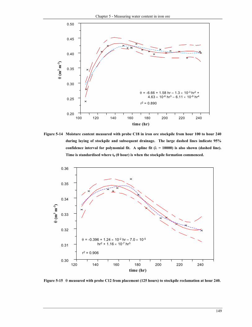
Chapter 5 - Measuring water content in iron ore
149
0.20
0.25
0.30
0.35
0.40
0.45
0.50
100 120 140 160 180 200 220 240
time (hr)
θ (m
3 m-3
)
θ = -6.66 + 1.58 hr – 1.3 × 10⁻³ hr2 +4.63 × 10⁻⁶ hr3 – 6.11 × 10⁻⁹ hr4
r2 = 0.890
Figure 5-14 Moisture content measured with probe C18 in iron ore stockpile from hour 100 to hour 240
during laying of stockpile and subsequent drainage. The large dashed lines indicate 95%
confidence interval for polynomial fit. A spline fit (λ = 10000) is also shown (dashed line).
Time is standardised where t0 (0 hour) is when the stockpile formation commenced.
0.30
0.31
0.32
0.33
0.34
0.35
0.36
120 140 160 180 200 220 240time (hr)
θ (m
3 m-3
)
θ = -0.396 + 1.24 × 10⁻² hr – 7.0 × 10⁻⁵
hr2 + 1.16 × 10⁻⁷ hr3
r2 = 0.906
Figure 5-15 θ measured with probe C12 from placement (125 hours) to stockpile reclamation at hour 240.

B.H. George – Measuring soil water content
150
0.37
0.38
0.39
0.40
0.41
0.42
0.43
0.44
0.45
0.46
0.47
20 60 100 140 180 220 260time (hr)
θ (m
3 m-3
)
θ = 0.337 + 1.82 × 10⁻³ hr – 1.0 × 10⁻⁵ hr2
+ 1.8 × 10⁻⁸ hr3
r2 = 0.906
Figure 5-16 θ measured with probe C11 from placement (40 hours) to stockpile reclamation at hour 240.
Maximum θ is obtained near hour 140 and maintained till reclamation indicating little
drainage with time.
0.27
0.28
0.29
0.30
0.31
0.32
0.33
0.34
0.35
0.36
0.37
0 50 100 150 200 250time (hr)
θ (m
3 m-3
)
θ = 0.278 + 1.58 × 10⁻³ hr – 1.0 × 10⁻⁵ hr2
+ 2.19 × 10⁻⁸ hr3
r2 = 0.859
Figure 5-17 θ measured with probe C04 from placement (5 hours) to stockpile reclamation at hour 240. θ
peaks around hour 100 with continues decline in reported θ till reclamation.

Chapter 5 - Measuring water content in iron ore
151
Drainage characteristics of the stockpile for three probes in the C-cross section are shown in
Figures 5-14 to 5-17. The probes are located at different heights approximately four meters,
stacker side, from the centre of the stockpile shown in Figure 5-8. Polynomial fits are shown
for all probes with appropriate spline fits carried out in JMP® (SAS Institute).
Results from probe C12 indicate an initial increase in θ followed by a constant decline. This is
to be expected as the water movement is dictated by gravity through the stockpile after the ore
is deposited. High measured hydraulic conductivity (Appendix 5-1) allows quick drainage
through the stockpile. Processed ore was dumped till hour 150 just prior to the peak in
measured θ.
Probes C11 and C04 exhibited a similar increase in θ with peak values at 140 h and 100 h
respectively. Calculated θ at probe C11 was noticeably higher than C12 (located directly
above C11 in the stockpile) and probe C04 (located below C11). This is most likely due to the
probe location, surrounded by “fines” (< 0.5 mm) ore material. θ remained constant (≈ 0.44
m3m-3) at C11. However, the probes above and below C11 declined with time. Again this
indicates congregation of fine material around the probe. Smaller material will retain water
due to smaller pore size distribution slowing drainage capability.
The TDR technique has a small ill-defined measurement area. Knight (1992) mathematically
derived the volume of measurement for unbalanced probes and the relative influence is shown
in Figure 1.9 (after Zegelin et al., 1989). Empirical derivation (by Baker and Lascano, 1989)
suggests a measurement cross-section area of 3500 to 4000 mm2 with the majority of influence
within 1000 mm2.
The material located closest to the TDR probe centre wire will have the greatest influence on
the EM wave with the measurement volume (m3) calculated (Zegelin et al., 1992):
2
2
−=
dRLV π (5-7)
Where L is the length of the probe (200 mm); d the centre wire diameter (3 mm) and; using the
assumption of Zegelin et al. (1992), R maximum radius of influence (0.05 m). The volume of
measurement with a 0.2 m long unbalanced probe is 0.00093 m3. The probe dimensions for a
radial influence of 0.05 m was considerably different with Zegelin et al.’s original study
(1989). If a maximum radius of measurement for this probe is actually 0.025 m then the
volume of measurement is even smaller by a three-fold factor (0.00035 m3; 350 ml).

B.H. George – Measuring soil water content
152
The small measurement volume is important in determination of θ for large (many thousands
of tonnes) stockpiles and is a limitation of the TDR technique for continued monitoring. Three
options exist for improving the measurement volume. Probes may have a different geometry
(larger probe diameter and spacing, Zegelin et al., 1989); probes may be longer in length (L in
equation 5-7); or more probes can be utilised in stockpile measurement.
5.5. CONCLUSIONS
Moisture content of iron ore can be determined by the TDR technique after calibration is
established. The influence of the iron content was found to not significantly affect the ability
of the TDR technique in determining moisture content. The ability to obtain the end-point
analysis contradicts the findings of Robinson et al. (1994) for an anthroposol soil with a high
(15 %) magnetite content. A good relationship was found between the laboratory and in situ
calibration for similar moisture contents, though the field calibration returned a significantly
higher intercept. This could be due to the change in in situ bulk density. The laboratory
calibration is a polynomial relationship with the TDR technique becoming more sensitive to
change in θ at higher moisture contents. Though the average stockpile ρb is higher (2.66 Mg
m-3) than found in most soil situations the calibration is robust to change experienced in field
conditions. Still, it is recommended that a calibration be conducted for each material.
For in situ θ determination extension cables are used to connect probes to the TDR instrument.
For measurement in stockpiles protection of the cable (RG-58) was necessary. A simple
process utilising common garden hose was found to successful. The extension cable affects
the EM travel and subsequent determination of the apparent dielectric by the automatic
software. A small but significant subtraction (-0.197) from the measured dielectric (Kam)
accounts for the effect of a 28 m extension cable. To ensure sustained measurement of
embedded probes some protection of the RG-58 coaxial extension is required. This can be
readily achieved in field situation by threading the coaxial cable through commonly available
garden hose.
The TDR technique can be successfully employed in determination of moisture content change
during stockpile formation and subsequent drainage period till reclamation is undertaken.
However, the small measurement volume of the TDR probes employed was susceptible to
immediate ore characteristics. In the stockpile creation, congregation of finer material was
observed and probes placed in this material measured comparatively higher moisture contents.

Chapter 5 - Measuring water content in iron ore
153
This sensitivity to local conditions may be overcome by increasing the probe dimensions
particularly length.
TDR is a potential alternative to other techniques currently used in continuous moisture
determination (Yip & Cutmore, 1993; Cutmore et al., 1996). However the invasive nature of
the probes limits the techniques’ capability for on-line measurement of the abrasive processed
iron ore during conveyor transport. An advantage of the TDR technique is the ability to
determined θ relationships inside stockpiles.
Chapter 6 – General discussion and conclusions
155
6.1. GENERAL DISCUSSION
Technology for the measurement of soil water content (θ) continues to develop rapidly. This
development, particularly during the last 15 years, has predominantly concentrated on
exploiting the difference between the dielectric of water (≈ 80) and the dielectric of the soil
matrix (≈ 3 - 5). Measurement of the combined components, the apparent dielectric (Ka), is
undertaken in the time-domain or the frequency-domain. There are, however, existing
limitations to measurement of soil water with the time-domain and frequency-domain
techniques. The understanding of the time-domain technique is better developed than
frequency-domain, as shown in the available literature (Chapter 1). The time-domain
technique is particularly well suited to near-surface, continued spatial measurements (e.g.
McBratney et al., 1997), though development of profile-based measurement (following the
initial work of Topp & Davis, 1985), has recently extended the application of time-domain
reflectometry (Hook & Livingstone, 1992; Ferre et al., 1997). Reducing the effectiveness of
the down-hole (profile) measurement, is the sensitivity of dielectric techniques to the effect of
air-gaps around the sensors (Dean et al., 1987; Knight et al., 1997). Though more sensitive to
the change in soil water content compared to the neutron moderation method, as shown in
Figure 4-8, the need for careful field installation cannot be over-emphasised. The sensitivity to
air-gaps around the sensors may continue to limit the application of dielectric techniques to
non-swelling soil.
Soil water content, reported with the time-domain reflectometry (TDR) technique, is still
widely based on use of Topp and his co-workers’ seminal research (Topp et al., 1980).
Different studies, especially in Europe (e.g. Roth et al., 1990; Roth et al., 1992), have
concentrated on developing a physical relationship based on the refractive index (Whalley,
1993). To develop a physically-based relationship between the Ka and θ, further
paramaterisation is required. Often this can be difficult to achieve in field conditions
(Jacobsen & Schjonning, 1993b). This difficulty in minimising the error associated with field
calibration, was experienced with bulk density measurement in a field calibration of the NMM
probe, shown in Chapter 4. Though not conclusive, results in Chapter 2 indicate a difference
in the equation of Topp et al. (1980) and measurement of θ in some typical Australian soil.
This is probably due to the effect of bound water on the measured apparent dielectric. The
potential effect of bound water, though recognised, is poorly understood, especially when
considered with other physical parameters. For example, the effect of particle size analysis

B.H. George – Measuring soil water content
156
(PSA) is considered by different researchers to have minimal or no significant impact on the
calibration of the TDR technique (Roth et al., 1990; Jacobsen & Schjonning, 1993a; and
Malicki et al., 1996). In their early work developing a “universal” calibration, Topp et al.
(1980) reported a difference in the response of a clay soil but still encompassed these results in
their calibration. The complex interaction between the PSA, specific surface area and the clay
mineralogy are difficult to define. Various models accounting for these parameters, or the
effect of bound water (as a surrogate of specific surface area or mineralogy) have yet to be
exploited in calibration of the TDR in some typical Australian soil. Bridge et al. (1996) found
measurement of θ based on the empirical calibration of Topp et al. (1980) to underestimate the
known θ in a Vertosol. I obtained similar results (Figure 2-3) in measurement of θ in a
saturated Vertosol where the (factory) supplied calibrations underestimated the gravimetrically
calculated θ. In explaining the underestimation of θ by determination with the “universal”
equation, three likely contributing reasons are: (i) the change in the imaginary component of
the dielectric as the electrical conductivity increases (White and Zegelin, 1995); (ii) a large
change in the bulk density due to the swell-shrink properties of the soil (Bridge et al., 1996)
and; (iii) the change in the bound-water component, especially the mono-molecular layer.
Bohl & Roth (1994) following the study of Dobson et al. (1985) consider the influence of
bound-water in some detail. Assuming a single molecular layer of water with a thickness of 3
× 10-10 m, Bohl & Roth (1994) found an optimal value (for their model) of bound water of 0.03
m3 m-3 (θbw) for mineral soil. Whether this value can be applied to different Australian soils is
yet to be seen and understood.
This returns us to the original problem where the interaction of the PSA, specific surface area
and mineralogy clouds development of a physical K(θ) relationship. The continued
parameterisation often leads to a small improvement in the attained calibration (Zegelin &
White, 1994). This desire to achieve a physical relationship by backward parameterisation for
different soil, persists (Yu et al., 1997). However, further calibration of the TDR technique,
particularly in heavy textured soil and specifically, soil that exhibits shrink-swell
characteristics, is certainly warranted.
With the TDR technique now widely used for θ measurement the use of extension cables
connecting the TDR unit to the buried probes is common. Most extension cables are coaxial
cables designed to minimise electromagnetic signal loss and often used in arrays of various
lengths. The determination of the Ka is shown in Section 2.4.7 to vary in different soil water
conditions and also vary with increasing length of extension cable. The relationship between
Chapter 6 – General discussion and conclusions
157
the change in reported Ka and the extension cable is not simply defined and the results
presented here (Figure 2-10) show the significance of the problem without fully explaining the
link between increasing extension cable length and Ka. The change in the reported Ka could be
linked to the decrease in the slope of the returning electromagnetic wave (Section 2.4.7.2).
Others have qualitatively observed the difference in the generated EM traces (Herkelrath et al.,
1991), deciding the measurement process was robust and there was no significant effect on the
reported Ka. As the use of the TDR technique increases, accounting for the effect of different
extension cable lengths connecting probes to the respective instrument will be important in
maintaining confidence in the measured Ka.
The application of dielectric techniques in measurement of soil water content and water
content in other porous media continues. Chapter 5 results show the ability of the TDR
technique to measure the water content of processed iron ore. The calibration is similar (in
form) to those developed by Zegelin & White (1994) for other ore-based products, and
encompasses the increasing imaginary component of the dielectric (K”) due to the
ferromagnetic properties of the iron ore. As opposed to Robinson et al. (1994), who
experienced difficulties in automatic determination of the EM wave end-point in a soil with
increased iron content, the TDR technique measured the changing moisture conditions
successfully (Figure 5-2) in the iron ore. The TDR technique is better adapted for water
content determination within the stockpile than other non-invasive techniques reported so far
(Yip & Cutmore, 1993), and has the potential for further development in process-based
industries.
During the field experiment (Chapter 4) the neutron moderation method performed well again
indicating that the technique is well suited for profile based measurements. The need for site,
or at least soil specific calibrations was again shown (Section 4.4.1) and this result is in
accordance with the findings of others (Hodgson & Chan, 1979; Greacen et al., 1981; Ruprecht
& Schoefield, 1990). The in situ calibration was more sensitive to the change in soil water
content compared to the “universal” calibration supplied by the manufacturer and this could be
due to the calibration process accounting for the in situ bulk density. The calibration results
need to be considered with some care as the range of soil water content, during calibration, was
limited and Cull (1979) showed that a large range of soil water content for calibration is
necessary for optimum calibration. For application of the calibration in the Chromosol, further
calibration should be carried out.
The NMM method, though less precise, due to the chaotic nature of radioactive decay (Table
3-1), and measuring a larger volume of soil, is a more robust technique for determination of θ,
B.H. George – Measuring soil water content
158
compared to TDR in attenuative soil. For TDR to be used in irrigation scheduling the
technique needs to consistently report the soil water content and not be limited in saturated
conditions if the EM wave attenuates and no end-point is derived. The FD sensors, the IH1
and the EnviroSCAN®, both reported measurement of θ in all soil water conditions
experienced. The operation of the IH1 probe will be limited due to the fragile nature of the
instrument (particularly the fibre optic cable), and the cost of batteries for operation. The
EnviroSCAN® system in these experiments operated well, reporting θ from saturated
conditions to small water contents (below refill point). Results from the field experiment
(Figure 4-12), indicate a good relationship between the increasing neutron count, with the
NMM, and the reported θ by the EnviroSCAN® FD system. However, the need for calibration
requires further research.
6.2. CONCLUSIONS
From the observations during the laboratory and field experiments with dielectric and neutron
moderation techniques I conclude:
♦ When using extension cables with the TDR technique for soil water content measurement,
a calibration for the effect of the extension cable is necessary. The calibration should
account for the type of cable, the different cable length and changing soil water content
conditions.
♦ The “universal” calibration developed by Topp et al. (1980) for the TDR technique can
underestimate the soil water content in heavy-textured soil. However, the increased
electrical conductivity often associated with clay soil in Australia, can lead to attenuation
of the electromagnetic wave causing difficulty in automatic end-point determination. This
difficulty can lead to large erroneous θ values and increased standard error of
measurement. Further, the increasing electrical conductivity can limit the application of
the TDR technique if there is no end-point reflection obtained.
♦ The TDR technique is capable, after calibration, of θ measurement in iron ore; and the
technique is well suited to measurement of water content in iron ore stockpiles.
♦ The IH1 down-hole frequency-domain probe is sensitive to the axial orientation of the
sensor in the access tube and rotation can lead to an error (bias) of 0.01 m3 m-3 (using the
factory supplied “universal” calibration).
Chapter 6 – General discussion and conclusions
159
♦ The frequency-domain technique is more sensitive to the change in soil water conditions
than the neutron moderation technique.
♦ An in situ calibration improves the sensitivity of the neutron moderation technique in a
Brown Chromosol compared to the factory supplied “universal” calibration. However, the
calibration procedure is limited by a large error in prediction (≈ 0.05 m3 m-3) and limited
water content range for determination.
6.3. FUTURE DIRECTIONS
Following the study undertaken in the different chapters, this component of my work is
probably the easiest to formulate. During the course of individual experiments the paths of
study more often diverge rather than converge. The study of the available dielectric techniques
is most interesting. Significant work during the late 1980s and early 1990s by Ian White, Steve
Zegelin and John Knight at CSIRO developed a good understanding of the TDR technique and
some applications. However, little research (apart from Bridge et al., 1996) has been
undertaken to develop a better understanding of the limitations of the TDR technique in heavy
textured Australian soil, particularly soil with high electrical conductivity and specific surface
area that actively shrinks and swells during drying and wetting cycles.
From my study (Chapter 2), of particular concern is the effect of extension cable on the
reported dielectric. Future research needs to explore the effect of the extension cable and
ideally develop a model for this effect on reported dielectric when using TDR instruments.
The ability of the TDR technique to measure different porous materials (Zegelin et al., 1994)
by sensor development and adaptation offers many opportunities for future study with the
technique. Of particular interest is the on-line measurement of ore material from mining
operations and other process-based industries. The key to development obviously remains the
ability to measure a change in dielectric and relate that to a relevant parameter. For θ
determination in iron ore one particular challenge is the ability to measure θ in a large sample
volume. To achieve this, development of TDR probe technology is required.
A rigorous in situ assessment of the frequency-domain technique is certainly warranted. Initial
results (Chapter 4) show a good relationship with the increase in θ measured by the NMM.
However there is little reported information on field operation of FD sensors in Australian soil
conditions. The measured frequency in water and air is important for the measurement of the
universal frequency. Concerns of increasing salinity and high temperature on the methodology

B.H. George – Measuring soil water content
160
of using the universal frequency approach need investigation. The field methodology for FD
technique should also consider the small measurement volume of FD sensors and the sensor
placement and susceptibility to change in the reported θ due to air gaps and sensor orientation.

Bibliography
161
Ahuja, L.R. & Nielsen, D.R., 1990. Field soil-water
relations. In: (eds. B.A.Stewart & D.R.Nielsen)
Irrigation of Agricultural Crops. Agronomy
Monograph No. 30., pp144-190.
Alharthi, A. & Lange, J., 1987. Soil water
saturation: dielectric determination. Water
Resources Research, 23:591-595.
Allyn, R.B. & Work, R.A., 1941. The availameter
and its use in soil moisture control: I. the
instrument and its use. Soil Science, 51:307-
321.
Anonymous, 1991. Soil moisture measurement with
time-domain reflectometry. The Campbell
Update, Campbell Scientific Newsletter, Utah,
USA. 2(1):1-2.
Anonymous, 1994. Moisture point: A new way to
measure soil moisture content - quickly, easily
and accurately. Environmental Sensors
Technical Specification Sheet for MP917,
British Columbia, Canada, pp2.
Anonymous, 1995. Berriquin Land and Water
Management Plan. Deniliquin, NSW, Australia.
Murray Irrigation pp120
ASTM, 1991. D-1556 Test method for density of
soil in place by the sand-cone method. In:
ASTM Annual Book of Standards. American
Society of Testing and Materials, 4.08:359-365.
Baker, J.M.,1990. Measurement of soil water
content. Remote Sensing Reviews, 5:263-279.
Baker, J.M. & Allmaras, R.R., 1990. System for
automating and multiplexing soil moisture
measurement by time-domain reflectometry.
Soil Science Society of America Journal, 54:1-6.
Baker, J.M. & Lascano, R.J., 1989. The spatial
sensitivity of time-domain reflectometry. Soil
Science, 147:378-384.
Baran, E., 1994. Use of time domain reflectometry
for monitoring moisture changes in crushed rock
pavements. Symposium and Workshop on Time-
domain Reflectometry in Environmental,
Infrastructure, and Mining Applications. United
States Bureau of Mines, SP 19-94, pp349-356.
Baumgartner, N., Parkin, G.W. & Elrick, D.E.,
1994. Soil water content and potential measured
by hollow time-domain reflectometry probe.
Soil Science Society of America Journal, 58:315-
318.
Bavel, C.H.M. van, 1962. Accuracy and source
strength in soil moisture neutron probes.
Proceeding of the Soil Science Society of
America, pp405.
Bavel, C.H.M. van, Nielsen, D.R. & Davidson,
J.M., 1961. Calibration and characteristics of
two neutron moisture probes. Soil Science
Society of America Proceedings, 25:329-334.
Bavel, C.H.M. van, Underwood, N. & Swanson,
R.W., 1956. Soil moisture measurement by
neutron moderation. Soil Science, 82:29-41.
Bell, J.P., Dean, T.J. & Hodnett, M.G., 1987. Soil
Moisture Measurement by an Improved
Capacitance Technique, Part II. Field
Techniques, Evaluation and Calibration.
Journal of Hydrology, 93:79-90.
Birchak, R.J., Gardner, C.G., Hipp, J.E. & Victor,
J.M., 1974. High dielectric constant microwave
probes for sensing soil moisture. Proceedings
IEEE, 62:93-98.
Blake, G.R. & Hartge, K.H., 1986. Bulk density.
In: (ed. A. Klute) Methods of Soil Analysis, Part
1. Physical and Mineralogical Methods.
Agronomy Monongraph No.9 (2nd edn). pp363-
375.
Boart Longyear CPN, 1995. CPN 503 DR
Hydroprobe Neutron Moisture Gauge, Oper-
ating Manual. Boart Longyear CPN; Martinez
CA USA. pp50.

B.H. George – Measuring soil water content
162
Bohl, H. & Roth, K., 1994. Evaluation of dielectric
mixing models to describe the θ(ε)-relation.
Symposium and Workshop on Time-domain
Reflectometry in Environmental, Infrastructure,
and Mining Applications. United States Bureau
of Mines, SP 19-94, pp309-319.
Bouyoucos, G.J., 1962. Hydrometer method
improved for making particle size analysis of
soils. Agronomy Journal. 54:464-465.
Boyer, J.S., 1982. Plant productivity and the
environment. Science, 218:443-448.
Brindley, G.W. & Brown, G., 1984. Crystal
Structures of Clay Minerals and their X-ray
Identification. Mineralogical Society, London
UK. pp495.
Brown, R.W. & Oosterhuis, D.M., 1992.
Measuring plant and soil water potentials with
thermocouple psychrometers: some concerns.
Agronomy Journal, 84:78-86.
Bridge, B.J., Sabburg, J., Habash, K.O., Ball, J.A.R.
& Hancock, N.H., 1996. The dielectric
behaviour of clay soils and its application to
time-domain reflectometry. Australian Journal
of Soil Research, 23:825-835.
Brisco, B., Pultz, T.J., Brown, R.J., Topp, G.C.,
Hares, M.A. & Zebchuk, W.D., 1992. Soil
moisture measurement using portable dielectric
probes and time-domain reflectometry. Water
Resources Research, 28:1339-1346.
Briscoe, R.D., 1984. Thermocouple psychrometers
for potential measurements. Proceedings NATO
Advanced Study Institute on "Advanced
Agricultural Instrumentation" Il Ciocco, Italy,
May 27 - June 9, 1984.
Bristow, K.L., 1998. Measurement of thermal
properties and water content of unsaturated
sandy soil using dual-probe heat-pulse probes.
Agricultural and Forest Meterology, 89:75-84.
Bristow, K.L., Campbell, G.S. & Calissendorff, K.,
1993. Test of heat-pulse probe for measuring
changes in soil water content. Soil Science
Society of America Journal, 57:930-934.
Bristow, K.L, Kluitenberg, G.J. & Horton, R.,1994.
Measurement of soil thermal properties with a
dual-probe heat-pulse technique. Soil Science
Society of America Journal, 58:1288-1294.
Brown, R.W. & Oosterhuis, D.M., 1992.
Measuring plant and soil water potentials with
thermocouple psychrometers: some concerns.
Agronomy Journal, 84:78-86.
Bull, C.R., 1991. Wavelength selection for near-
infrared reflectance moisture meters. Journal of
Agricultural Engineering Research, 49:113-125.
Burrows, W.C. & Kirkham, D., 1958. Measurement
of field capacity with a neutron meter. Soil
Science Society Proceedings, (United States of
America) pp103-105.
Buss, P., 1994. Continuous monitoring of moisture
in hardwood plantations irrigated with secondary
treated effluent. AWWA Recycled Water
Seminar, Newcastle Australia. pp180-189.
Campbell, G.S., 1988. Soil water potential
measurement: an overview. Irrigation Science,
9:265-273.
Campbell, G.S., Calissendorff, C. & Williams, J.H.,
1991. Probe for measuring soil specific heat
using a heat-pulse method. Soil Science Society
of America Journal, 55:291-293.
Campbell, G.S. & Gee, G.W., 1986. Water
potential: miscellaneous methods. In: (ed. A.
Klute) Methods of Soil Analysis, Part 1.
Physical and Mineralogical Methods.
Agronomy Monongraph No.9 (2nd edn). pp619-
633.
Campbell, J.E., 1990. Dielectric properties and
influence of conductivity in soils at one to fifty
Bibliography
163
megahertz. Soil Science Society of America
Journal, 54:332-341.
Carmer, S.G. & Walker, W.M., 1982. Baby Bear’s
dilema: A statistical tale., Agronomy Journal,
74:122-124.
Carneiro, C. & De Jong, E., 1985. In situ
determination of the slope of the calibration
curve of a neutron probe using a volumetric
technique. Soil Science, 139:250-254.
Carrow, R.N., Shearman, R.C. & Watson, J.R.,
1990. Turfgrass. In: (eds. B.A. Stewart & D.R.
Nielsen) Irrigation of Agricultural Crops. SSSA
Monograph No. 30. pp889-919.
Cassel, D.K., Kachanoski, R.G. & Topp, G.C.,
1994. Practical considerations for using a TDR
cable tester. Soil Technology, 7:113-126.
Chanasyk, D.S. & McKenzie, R.H., 1986. Field
calibration of a neutron probe. Canadian
Journal of Soil Science, 66:173-176.
Childs, E.C., (1940). The use of soil moisture
characteristics in soil studies. Soil Science,
50:239-252.
Colman, E.A. & Hendrix, T.M., 1949. The
fibreglass electrical soil-moisture instrument.
Soil Science, 67:425-438.
Corey, A.T. & Klute, A., 1985. Application of the
potential concept to soil water equilibrium and
transport. Soil Science Society of America
Journal, 49:3-11.
Cornish, P.M., Laryea, K. & Bridge, B.J., 1972. A
nondestructive method of following moisture
content and temperature changes in soils using
thermistsors. Soil Science, 115:309-314.
Cresswell, H.P.,1993. Evaluation of the portable
pressure transducer technique for measuring
field tensiometers. Australian Journal of Soil
Research, 31:397-406.
Cull, P.O., 1979. Unpublished PhD thesis.
University of Armidale, NSW Australia. pp241.
Cull, P.O., 1992. Irrigation scheduling - techniques
and profitability. National Irrigation
Convention Proceedings. Melbourne, Australia.
pp131-170.
Cullen, S.J. & Everett, L.G., 1995. Estimating the
storage capacity of the vadose zone. In: (eds.
L.G. Wilson, L.G. Everett & S.J. Cullen)
Handbook of Vadose Zone Characterization and
Monitoring. CRC Press, Baco Raton, Fl USA.
pp159-176.
Cummings, R.W. & Chandler, R.F., 1940. A field
comparison of the electrothermal and gypsum
block electrical resistance methods with the
tensiometer method for estimating soil moisture
in situ. Soil Science Society of America
Proceedings, 5:80-85.
Cutmore, N.G., Eberhardt, J.E., Sowerby, B.D. &
Watt, J.S., 1996. On-line measurement of
composition for the Australian mineral and
energy industries. IEEE Instrumentation and
Measurement Technology Conference, Brussels,
Belgium; June 4-6 1996. pp330-334.
Dalton, F.N., 1992. Development of time-domain
reflectometry for measuring soil water content
and bulk soil electrical conductivity. In: (eds.
G.C. Topp, W.D. Reynolds & R.E. Green)
Advances in Measurement of Soil Physical
Properties: Bringing Theory into Practice.
pp143-168.
Dasberg, S., Alksnis, H., Daniel, P., Kalma, J.D.
and Zegelin, S.J., 1995. Calibration of the
"moisture point" TDR system. Cooperative
research Centre for Catchment Hydrology
Report 95/4 (Australia) pp1-15.
Dean, T.J., Bell, J.P. & Baty, A.J.B., 1987. Soil
Moisture Measurement by an Improved
Capacitance Technique. Part I. Sensor Design
B.H. George – Measuring soil water content
164
and Performance. Journal of Hydrology, 93:67-
78.
Dickey, G.L., Allen, R.G., Wright, J.L., Murray,
N.R., Stone, J.F. & Hunsaker, D.J., 1993. Soil
bulk density sampling for neutron gauge
calibration. Proceedings of the ASCE National
Conference on Irrigation and Drainage
Engineering, Park City, UT, USA.
Didcot , 1992. Capacitance Soil Moisture Probe
Type IH1 - Provisional Manual. Didcot
Instrument Company, Oxford, UK. pp 15.
Dirksen, C. & Dasberg, S., 1993. Improved
calibration of time-domain reflectometry soil
water content measurements. Soil Science
Society of America Journal, 57:660-667.
Dobson, M.C., Ulaby, F.T., Hallikainen, M.T. & El-
Rayes, M.A., 1985. Microwave dielectric
behaviour of wet soil - Part II: Dielectric mixing
models. Institution of Electrical and Electronic
Engineers Transactions on Geoscience and
Remote Sensing, GE-23, 35-46.
Drake, F.H., Pierce, G.W. & Dow, M.T., 1930.
Measurement of the Dielectric Constsant and
Index of Refractions of Water and Aqueous
Solutions of KCL at High Frequencies. Physical
Reviews, 35:613-622.
Evett, S.R., 1994. TDR-temperature arrays for
analysis of field soil thermal properties.
Symposium and Workshop on Time-domain
Reflectometry in Environmental, Infrastructure,
and Mining Applications. United States Bureau
of Mines, SP 19-94, pp320-327.
Evett, S.R. & Steiner, J.L., 1995. Precision of
neutron scattering and capacitance type soil
water content gauges from field calibration. Soil
Science Society of America Journal, 59:961-968.
Falkiner, R.A. & Smith, C.J., 1997. Changes in soil
chemistry in effluent-irrigated Pinus radiata and
Eucalyptus grandis plantations. Australian
Journal of Soil Research. 35:131-147.
Fellner-Feldegg, H., 1969. The measurement of
dielectrics in the time-domain. Journal of
Physical Chemistry, 73:616-623.
Ferre, P.A., Rudolph, D.L. & Kachanoski, R.G.,
1996. Spatial averaging of water content by
time-domain reflectometry: implications for twin
rod probes with and without dielectric coatings.
Water Resources Research, 32(2):271-279.
Fleming, R.L., Black, T.A. & Eldridge, N.R., 1993.
Water content, bulk density, and coarse fragment
content measurement in forest soils. Soil
Science Society of America Journal, 57:261-270.
Fredlund, D.G., 1992. Background, theory, and
research related to the use of thermal conduct-
ivity sensors for matric suction measurement.
In: (eds. G.C. Topp, W.D. Reynolds & R.E.
Green) Advances in Measurement of Soil
Physical Properties: Bringing Theory into
Practice. SSSA Special Publication No 30.
pp249-261.
Frueh, W.T. & Hopmans, J.W., 1997. Soil moisture
calibration of a TDR multilevel probe in gravely
soil. Soil Science, 162(8):554-565.
Fundinger, R., Kohler, K. & Stacheder, M., 1995.
Measurement of material and soil moisture with
the TRIME-method. TRIME Product Guide,
IMKO GMbH, Ettlingen, Germany.
Gardner, W. & Kirkham, D., 1952. Determination
of soil moisture by neutron scattering. Soil
Science, 73:391-401.
Gardner, W., Israelsen, O.W., Edlefsen, N.E. &
Clyde, D., 1922. The capillary potential
function and its relation to irrigation practice.
Physical Revue, 20:196-204.
Gardner, W.H., 1986. Water content. In: (ed. A.
Klute) Methods of Soil Analysis, Part 1.
Bibliography
165
Physical and Mineralogical Methods.
Agronomy Monograph No.9 (2nd edn). pp493-
544.
Gaskin, G.J. & Miller, J.D., 1996. Measurement of
soil water content using a simplified impedance
measuring technique. Journal of Agricultural
Engineering Research, 63:153-160.
Gee, G.W. & Bauder, J.W., 1986. Particle-size
analysis. In: (ed: A.Klute) Methods of Soil
Analysis, Part 1. Physical and Mineralogical
Methods. Agronomy Monongraph no.9 (2nd
edn). pp383-411.
Gee, G.W., Silver, J.F. & Borchert, H.R., 1976.
Radiation hazard from Americium-Beryllium
neutron moisture probes. Soil Science Society of
America Journal, 40:492-494.
Greacen, E.L., Correll, R.L., Cunningham, R.B.,
Johns, G.G. & Nicolls, K.D., 1981. Calibration.
In: (ed. E.L. Greacen) Soil Water Assessment by
the Neutron Method. CSIRO, Melbourne, pp
50-72.
Greacen, E.L. & Hignett, C.T., 1979. Sources of
bias in the field calibration of a neutron meter.
Australian Journal of Soil Research, 17:405-
415.
Greacen, E.L. & Schrale, G., 1976. The effect of
bulk density on neutron meter calibration.
Australian Journal of Soil Research, 17:159-
169.
Green, R.E. & Topp, G.C., 1992. Survey of use of
field methods for measuring soil hydraulic
properties. In: (eds. G.C. Topp, W.D. Reynolds
& R.E. Green) Advances in Measurement of Soil
Physical Properties: Bringing Theory into
Practice. SSSA Special Publication No 30,
pp281-288.
Guerra, F., 1974. Handling of wet, sticky ores.
Proceedings from International Symposium on
Transport and Handling of Minerals. Miller
Freeman Publishing Inc., San Francisco, CA,
USA. pp175-200.
Halbertsma, J., van den Elsen, E., Bohl, H., &
Skierucha, W., 1995. Temperature effects on
TDR determined soil water content.. In: (eds.
L.W. Petersen & O.H. Jacobsen), Proceedings
from the Symposium on Time-domain
reflectometry applications in soil science.
Research Centre Foulum, Denmark, September
16, 1994. SP Report Danish Institute of Plant
and Soil Science, 11(3):35-37.
Hanks, R.J., 1992. Water Potentials. In: Applied soil
physics. Soil water and temperature
applications. Springer-Verlag, New York.
pp176.
Hanson, B.R. & Dickey, G.L., 1993. Field practices
affect neutron moisture meter accuracy.
California Agriculture, November-December
1993, pp29-31.
Haverkamp, R., Vauclin, M. & Vachaud, G., 1984.
Error analysis in estimating soil water content
from neutron probe measurements: 1. local
standpoint. Soil Science, 137:78-90.
Heimovaara, T.J., 1993. Design of triple-wire time-
domain reflectometry probes in practice and
theory. Soil Science Society of America Journal,
57:1410-1417.
Heimovaara, T.J., 1994a. Frequency domain
analysis of time domain reflectometry
waveforms. 1. Measurement of the complex
dielectric permittivity of soils. Water Resources
Research, 30:189-199.
Heimovaara, T.J., 1994b. Frequency domain
analysis of time domain reflectometry wave-
forms. 2. A four-component complex dielectric
mixing model for soils. Water Resources
Research, 30:200-209.
Heimovaara, T.J. & Bouten, W., 1990. A computer
controlled 36-channel time-domain reflect-
B.H. George – Measuring soil water content
166
ometry system for monitoring soil water
contents. Water Resources Research, 26:2311-
2316.
Heimovaara, T.J, Focke, A.G., Bouten, W. &
Verstraten, J.M., 1995. Assessing temporal
variations in soil water composition with time
domain reflectometry. Soil Science Society of
America Journal, 59:689-698.
Heimovaara, T.J. & de Water, E., 1993. A
computer controlled TDR system for measuring
water content and bulk electrical conductivity of
soils. Report No. 41, Laboratory of Physical
Geography and Soil Science, Universtiy of
Amsterdam, pp27.
Hendrickx, J.M.H., Nieber, J.L. & Siccama, P.D.,
1994. Effect of tensiometer cup size on field
soil water tension variability. Soil Science
Society of America Journal, 58:309-315.
Herkelrath, W.N., Hamburg, S.P. & Murphy, F.,
1991. Automatic, real-time monitoring of soil
moisture in a remote field area with time-domain
reflectometry. Water Resources Research,
27:857-864.
Hilhorst, M,A. & Dirksen, C., 1994. Dielectric
water content sensors: time-domain versus
frequency domain. Symposium and Workshop
on Time-domain Reflectometry in Environ-
mental, Infrastructure, and Mining App-
lications. United States Bureau of Mines
Special Publication SP 19-94, pp23-33.
Hillel, D.K., 1991. Out of the Earth. The Free
Press. New York, USA.
Hipp, J.E., 1974. Soil Electromagnetic Parameters
as Functions of Frequency, Soil Density, and
Soil Moisture. Proceedings IEEE, 62:98-103.
Von Hippel, A.T. (ed.), 1954. Dielectric Materials
and Applications. MIT Press, Cambridge, USA.
Hodgson, A.S. & Chan, K.Y., 1979. Field
calibration of a neutron moisture meter in a
cracking grey clay. Irrigation Science, 8:233-
244.
Hodnett, M.G. & Bell, J.P., 1991. Neutron Probe
Standards: Transport Shields or a Large Drum of
Water? Soil Science, 51:113-120.
Hoelscher, J.R., Nuttle, W.K. & Harvey, J.W.,1993.
The calibration and use of pressure transducers
in tensiometer systems. Hydrological Processes,
7:205-211.
Holmes, J.W., 1956. Calibration and the field use
of the neutron scattering method of measuring
soil water content. Australian Journal of
Applied Science, 7:45-58.
Holmes, J.W., 1966. Influence of bulk density of
the soil on neutron moisture meter calibration.
Soil Science.
Hook, W.R. & Livingston, N.J., 1995. Propagation
velocity errors in time-domain refletometry
measurements of soil water. Soil Science
Society of America Journal, 59:92-96.
Hook, W.R. & Livingston, N.J., 1996. Errors in
converting time domain reflectometry
measurements of propagation velocity to
estimates of soil water content. Soil Science
Society of America Journal, 59:35-41.
Hook, W.R., Livingston, N.J., Sun, Z.J. & Hook,
P.B., 1992. Remote diode shorting improves
measurement of soil water by time-domain
reflectometry. Soil Science Society of America
Journal, 56:1384-1391.
Isbell, R.F., 1996. The Australian Soil
Classification. CSIRO Publishing, Colling-
wood, Australia. pp 143.
Jackson, T.J., 1988. Research toward an operational
passive microwave remote sensing system for

Bibliography
167
soil moisture. Journal of Hydrology, 102:95-
112.
Jackson, T.J., Schmugge, J. & Engman, E.T., 1996.
Remote sensing applications to hydrology: soil
moisture. Hydrological Sciences, 41(4):517-
530.
Jacobsen O.H, & Schjonning P., 1993a. A
laboratory calibration of time-domain
reflectometry for soil water measurement
including effects of bulk density and texture.
Journal of Hydrology, 151:147-157.
Jacobsen, O.H. & Schjonning, P., 1993b. Field
evaluation of time-domain reflectometry for soil
water measurements. Journal of Hydrology,
151:159-172.
Janoo, V., Berg, R.L., Simonsen, E. & Harrison, A.,
1994. Seasonal changes in moisture content in
airport and highway pavements. Symposium and
Workshop on Time-domain Reflectometry in
Environmental, Infra-structure, and Mining
Applications. United States Bureau of Mines,
SP 19-94, pp357-363.
Jayawardane, N.S., Meyer, W.S. & Barrs, H.D.,
1983. Moisture measurement in a swelling clay
soil using neutron moisture meters. Australian
Journal of Soil Research. 22:109-117.
Johnson, R. & Borough, C., 1992. Irrigating trees
with pulpmill effluent - a living tribute to the late
Wilf Crane. ANM Special Liftout No. 21, Winter
1992, 15(2).
Kabat, P. & Beekma, J., 1994. Water in the
unsaturated zone. In: (eds. H.P. Ritzema)
Drainage Principles and Applications. IRLI
Publication 16, pp383-434.
Kachanoski, R.G., Pringle, E. & Ward, A., 1992.
Field Measurements of Solute Travel Times
Using Time Domain Reflectometry. Soil
Science Society of America Journal, 56:47-52.
Kachanoski, R.G., Thony, J.L., Vauclin, M.,
Vauchaud, G. & Laty, R., 1994. Measurement
of solute transport during constant infiltration
from a point source. Soil Science Society of
America Journal, 58:304-309.
Kamgar, A., Hopmans, J.W., Wallender, W.W. &
Wendroth, O., 1993. Plotsize and sample
number for neutron probe measurements in
small field trials. Soil Science, 156:213-224.
Kempthorne, O. & Allmaras, R.R., 1986. Errors
and variability of observations. In: (ed: A.Klute)
Methods of Soil Analysis, Part 1. Physical and
Mineralogical Methods. Agronomy Monograph
No.9 (2nd edn). pp1-31.
Kendall, M. & Stewart, A., 1977. The Advanced
Theory Of Statistics - Distribution Theory.
Charles Griffin & Company, Vol 4., pp261.
Khosla, R. & Persaud, N., 1997. Performance of a
non-nuclear resonant frequency capacitance
probe. I. calibration and field testing.
Communications in Soil Science & Plant
Analysis. 28:(15&16)1333-1345.
Kim, D.J., Vanclooster, M., Feyen, J., & Vereecken,
H., 1998. Simple linear model for calibration of
time domain reflectometry measurements on
solute concentration. Soil Science Society of
America Journal, 62:83-89.
Klute, A., 1986. Water retentiaon: laboratory
methods. In: (ed. A. Klute) Methods of Soil
Analysis, Part 1. Physical and Mineralogical
Methods. Agronomy Monongraph No.9 (2nd
edn). pp635-662.
Knight, J.H., 1991. Discussion of "The spatial
sensitivity of time-domain reflectometry" by
J.M.Baker & R.J.Lascano. Soil Science,
151:254-255.
Knight, J.H., 1992. Sensitivity of time-domain
reflectometry measurements to lateral variations
B.H. George – Measuring soil water content
168
in soil water content. Water Resources
Research, 28:2345-2352.
Knight, J.H., Ferre, P.A., Rudolph, D.L. &
Kachanoski, R.G., 1997. A numerical analysis
of the effects of coatings and gaps upon relative
dielectric permittivity measurement with time
domain reflectometry. Water Resources
Research, 33(6):1455-1460.
Koppi, T. (ed), 1995. Soil Properties & Processes.
Soil Science 2 course notes, University of
Sydney, NSW Australia.
Kraus, J.D., 1984. Waveguides and resonators. In:
Electromagnetics. McGraw-Hill Book Co,
Singapore. pp 534-611.
Lal, R., 1974. The effect of soil texture and density
on the neutron probe calibration for some
tropical soils. Soil Science, 117:183-190.
Ledieu, J., de Ridder, P., de Clarck, P. &
Dautrebande, S., 1986. A method of measuring
soil moisture by time-domain reflectometry.
Journal of Hydrology, 88:319-328.
Look, B.G., Reeves, I.N. & Williams, D.J., 1994.
Field experiments using time domain
reflectometry for monitoring moisture changes
in road embankments and pavements.
Symposium and Workshop on Time-domain
Reflectometry in Environmental, Infrastructure,
and Mining Applications. United States Bureau
of Mines, SP 19-94, pp374-385.
Loon, W.K.P. van, Perfect, E., Groenevelt, P.H. &
Kay, B.D., 1991. Application of dispersion
theory to time-domain reflectometry in soils.
Transport in Porous Media, 6:391-406.
Lowery, B., Datiri, B.C. & Andraski, B.J., 1986.
An electrical readout system for tensiometers.
Soil Science Society of America Journal, 50:494-
496.
Malicki, M., 1983. A capacity meter for the
investigation of soil moisture dynamics. Zesty
Problemowe Postepow Nauk Rolniczych, pp
201-214.
Malicki, M., 1990. A reflectometric (TDR) meter of
moisture content in soils and other capillary-
porous materials. Zeszyty Problemowe
Postepow Nauk Rolniczych, 388:107-114.
Malicki, M.A., Plagge, R., Renger, M. & Walczak,
R.T., 1992. Application of time-domain
reflectometry (TDR) soil moisture miniprobe for
the determination of unsaturated soil water
characteristics from undisturbed soil cores.
Irrigation Science, 13:65-72.
Malicki, M.A., Plagge, R. & Roth, C.H., 1996.
Improving the calibration of dielectric TDR soil
moisture determination taking into account the
solid soil. European Journal of Soil Science,
47:357-366.
Malicki, M.A. & Skierucha, W.M., 1989. A
manually controlled TDR soil moisture meter
operating with 300 ps rise-time needle pulse.
Irrigation Science, 10:153-163.
Malicki, M.A., Walczak, R.T., Koch, S. & Fluher,
H., 1994. Determining Soil Salinity from
Simultaneous Readings of its Electrical
Conductivity and Permittivity using TDR.
Symposium and Workshop on Time-domain
Reflectometry in Environmental, Infra-structure,
and Mining Applications. United States Bureau
of Mines, SP 19-94, pp328-336.
McBratney, A.B., Whelan, B.W. & Shatar, T.M.,
1997. Variability and uncertainty in spatial,
temporal and spatiotemporal crop-yield and
related data. Precision Agriculture: Spatial and
Temporal Variability of Environmental Quality.
Wiley Chichester, Ciba Foundation Symposium
210; pp141-160.

Bibliography
169
McCann, I.R., Stark, J.C. & King, B.A., 1992.
Evaluation and interpretation of the crop water
stress index for well watered potatoes.
American Potato Journal, 69:831-841.
McKenzie, D.C., Hucker, K.W., Morthorpe, L.J. &
Baker, P.J., 1990. Field calibration of a neutron-
gamma probe in three agriculturally important
soils of the lower Macquarie valley. Australian
Journal of Experimental Agriculture, 30:115-
122.
McIntyre, D.S. & Barrow, K.J., 1972. An improved
sampling method for small undisturbed cores.
Soil Science, 114:239-141.
Mead, R., Curnow, R.N. & Hasted, A.M., 1993.
Statistical Methods in Agriculture and
Experimental Biology. 2nd edition. Chapman &
Hall, London, UK. pp415.
Mead, R.M., Ayars, J.E. & Liu, J., 1995.
Evaluating the influence of soil texture, bulk
density and soil water salinity on a capacitance
probe calibration. ASAE Summer Meeting,
Chicago Il, USA. June 18-23, 1995. ASAE
paper 95-3264.
Mead, R.M., Paltineanu, I.C., Ayars, J.E. & Liu, J.,
1994. Capacitance probe use in soil water
measurements. ASAE Summer Meeting, Kansas
City MO, USA. June 20-22, 1994. ASAE paper
942122.
Monteith, J.L. & Owen, P.C., 1958. Journal of
Scientific Instruments. 35:443-
Moutonnet, P., Pluyette, E., El Mourabit, N. &
Couchat, P., 1988. Measuring the spatial
variability of soil hydraulic conductivity using
an autometic neutron moisture gauge. Soil
Science Society of America Journal, 52:1521-
1526.
Mullins, C.E., 1977. Magnetic suseptibility of the
soil and its significance in soil science – a
review. Journal of Soil Science, 28:223-246.
Nadler, A. & Lapid, Y., 1996. An improved
capacitance sensor for in situ monitoring of soil
moisture. Australian Journal of Soil Research,
34:361-368.
Newman, A.C.D., 1983. The specific surface of
soils determined by water sorption. Journal of
Soil Science, 34:23-32.
Nieber, J.L., Baker, J.M. & Spaans, J.A., 1991.
Evaluation of soil water sensors in frozen soils.
Road & Airport Pavement Response Monitoring
Systems Conference Proceedings. TCCRE/
ASCE West Lebanon NH/Sept 12-16 1991.
pp168-181.
Nissan, H.H., Moldrup, P. & Henriksen, K., 1998.
High-resolution time domain reflectometry coil
probe for measuring soil water content. Soil
Science Society of America Journal, 62:1203–
1211.
Nutting, P.G., 1943. Some standard thermal
dehydration curves of minerals. U.S. Geological
Survey Professional Paper197-E.
O'Leary, G.J. & Incerti, M., 1993. A field
comparison of three neutron moisture meters.
Australian Journal of Experimental Agriculture,
33:59-69.
Olgaard, P.L. & Haahr, V., 1967. Comparative
experimental and theoretical investigations of
the DM neutron moisture probe. Nuclear
Engineering Design, 5:311-324.
Olgaard, P.L. & Haahr, V., 1968. On the sensitivity
of subsurface neutron moisture gauges to
variations in bulk density. Soil Science, 105:62-
64.
Oliviera, I.B., Demond, A.H. & Salehzadeh, A.,
1996. Packing sands for the production of
homogeneous porous media. Soil Science
Society of America Journal, 60:49-53.

B.H. George – Measuring soil water content
170
Oostrum, M., Hofstee, C., Dane, H. & Lenhard,
R.J., 1998. Single-source gamma radiation pro-
cedures for improved calibration and
measurements in porous media. Soil Science,
163(8)646-656.
Ould Mohamed, S., Bertuzzi, P., Bruand, A.,
Raison, L. & Bruckler, L., 1997. Field
evaluation and error analysis of soil water
content measurement using the capacitance
probe method. Soil Science Society of Amercia
Journal, 61:399-408.
Paetzold, R.F., Matzkanin, G.A. & De Los Santos,
A., 1985. Surface soil water content
measurement using pulsed nuclear magnetic
resonance techniques. Soil Science Society of
America Journal, 49:537-540.
Paltineanu, I.C. & Starr, J.L., 1997. Real-time soil
water dynamics using multisensor capacitance
probes: laboratory calibration. Soil Science
Society of America Journal, 61:1576-1585.
Payne, D., 1988. The behaviour of water in soil. In:
(ed. A. Wild) Russel’s Soil Conditions and Plant
Growth. pp991.
Pepin, S., Livingston, N.J. & Hook, W.R., 1995.
Temperature-dependent measurement errors in
time-domain reflectometry determinations of soil
water. Soil Science Society of America Journal,
59:38-43.
Perdok, U.D., Kroesbergen, B. and Hilhorst, M.A.,
1996. Influence of gravimetric water content
and bulk density on the dielectric properties of
soil. European Journal of Soil Science, 47:367-
371.
Persson, M. & Berndtsson R., 1998. Texture and
electrical conductivity effects on temperature
dependency in time domain reflectometry. Soil
Science Society of America Journal, 62:887-893.
Phene, C.J., Clark, D.A., Cardon, G.E. & Mead,
R.M., 1992. Soil matric potential sensor research
and applications. In: (eds. G.C. Topp, W.D.
Reynolds & R.E. Green) Advances in
Measurement of Soil Physical Properties:
Bringing Theory into Practice. SSSA Special
Publication No 30. pp263-280.
Polglase, P.J., Tomkins, D., Stewart, L.G. &
Falkiner, R.A., 1995. Mineralization and
leaching of nitrogen in an effluent-irrigated pine
plantation. Journal of Environmental Quality,
24:911-920.
Prebble et al. 1981
Puckett, W.E. & Dane J.H., 1981. Testing
tensiometers by a vacuum method. Soil Science,
132:48-50.
Rasmussen, T.C. & Rhodes, S.C., 1995. Energy-
related methods:psychrometers. In: (eds. L.G.
Wilson, L.G. Everett & S.J. Cullen) Handbook
of vadose zone characterization and monitoring.
CRC Press, Boca Raton, Fl USA. pp329-341.
Rawlins, S.L. & Campbell, G.S., 1986. Water
potential: thermocouple psychrometry. In: (ed.
A. Klute) Methods of soil analysis. Part 1 -
Physical and mineralogical methods. Agronomy
Monograph No. 9 part 1. pp597-618.
Reece, C.F., 1996. Evaluation of a line heat
dissipation sensor for measuring soil matric
potential. Soil Science Society of America
Journal, 60:1022-1028.
Reynolds, S.G., 1970a. The gravimetric method of
soil moisture determination, part I. A study of
equipment, and methodological problems.
Journal of Hydrology, 11:258-273.
Reynolds, S.G., 1970b. The gravimetric method of
soil moisture determination, part II. Typical
required sample sizes and methods of reducing
variability. Journal of Hydrology, 11:274-287.
Reynolds, S.G., 1970c. The gravimetric method of
soil moisture determination, part III. An
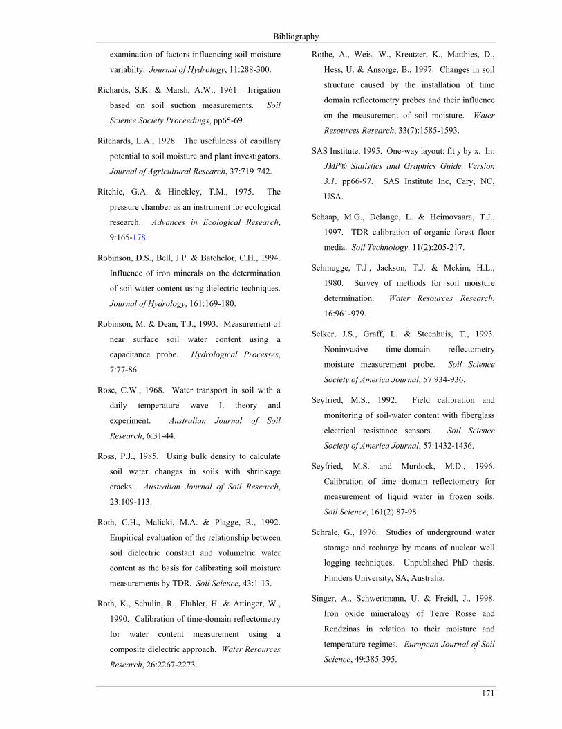
Bibliography
171
examination of factors influencing soil moisture
variabilty. Journal of Hydrology, 11:288-300.
Richards, S.K. & Marsh, A.W., 1961. Irrigation
based on soil suction measurements. Soil
Science Society Proceedings, pp65-69.
Ritchards, L.A., 1928. The usefulness of capillary
potential to soil moisture and plant investigators.
Journal of Agricultural Research, 37:719-742.
Ritchie, G.A. & Hinckley, T.M., 1975. The
pressure chamber as an instrument for ecological
research. Advances in Ecological Research,
9:165-178.
Robinson, D.S., Bell, J.P. & Batchelor, C.H., 1994.
Influence of iron minerals on the determination
of soil water content using dielectric techniques.
Journal of Hydrology, 161:169-180.
Robinson, M. & Dean, T.J., 1993. Measurement of
near surface soil water content using a
capacitance probe. Hydrological Processes,
7:77-86.
Rose, C.W., 1968. Water transport in soil with a
daily temperature wave I. theory and
experiment. Australian Journal of Soil
Research, 6:31-44.
Ross, P.J., 1985. Using bulk density to calculate
soil water changes in soils with shrinkage
cracks. Australian Journal of Soil Research,
23:109-113.
Roth, C.H., Malicki, M.A. & Plagge, R., 1992.
Empirical evaluation of the relationship between
soil dielectric constant and volumetric water
content as the basis for calibrating soil moisture
measurements by TDR. Soil Science, 43:1-13.
Roth, K., Schulin, R., Fluhler, H. & Attinger, W.,
1990. Calibration of time-domain reflectometry
for water content measurement using a
composite dielectric approach. Water Resources
Research, 26:2267-2273.
Rothe, A., Weis, W., Kreutzer, K., Matthies, D.,
Hess, U. & Ansorge, B., 1997. Changes in soil
structure caused by the installation of time
domain reflectometry probes and their influence
on the measurement of soil moisture. Water
Resources Research, 33(7):1585-1593.
SAS Institute, 1995. One-way layout: fit y by x. In:
JMP® Statistics and Graphics Guide, Version
3.1. pp66-97. SAS Institute Inc, Cary, NC,
USA.
Schaap, M.G., Delange, L. & Heimovaara, T.J.,
1997. TDR calibration of organic forest floor
media. Soil Technology. 11(2):205-217.
Schmugge, T.J., Jackson, T.J. & Mckim, H.L.,
1980. Survey of methods for soil moisture
determination. Water Resources Research,
16:961-979.
Selker, J.S., Graff, L. & Steenhuis, T., 1993.
Noninvasive time-domain reflectometry
moisture measurement probe. Soil Science
Society of America Journal, 57:934-936.
Seyfried, M.S., 1992. Field calibration and
monitoring of soil-water content with fiberglass
electrical resistance sensors. Soil Science
Society of America Journal, 57:1432-1436.
Seyfried, M.S. and Murdock, M.D., 1996.
Calibration of time domain reflectometry for
measurement of liquid water in frozen soils.
Soil Science, 161(2):87-98.
Schrale, G., 1976. Studies of underground water
storage and recharge by means of nuclear well
logging techniques. Unpublished PhD thesis.
Flinders University, SA, Australia.
Singer, A., Schwertmann, U. & Freidl, J., 1998.
Iron oxide mineralogy of Terre Rosse and
Rendzinas in relation to their moisture and
temperature regimes. European Journal of Soil
Science, 49:385-395.
B.H. George – Measuring soil water content
172
Skaling, W., 1992. Trase: a product history. In:
(eds. G.C. Topp, W.D. Reynolds & R.E. Green)
Advances in Measurement of Soil Physical
Properties: Bringing Theory into Practice.
SSSA Special Publication No 30, pp169-185.
Smith-Rose, R.L., 1933. The electrical properties of
soils for alternating currents at radio frequencies.
Proceedings of Royal. Society London.
140:359-377.
Soane, B.D & Calissendorff, C., 1961. The rapid
determination of soil water content using the
carbide method. Rhodesian Agricultural
Journal, 58:386-392.
Soilmoisture Equipment Corporation, 1993. Trase
system I - operating instructions. Soilmoisture
Equipment Corporation Incorporated, Santa
Barbara CA, USA.
Spaans, E.J.A. & Baker, J.M., 1992. Calibration of
Watermark soil moisture sensors for soil matric
potential and temperature. Plant and Soil,
143:213-217.
Spain, A.V., Isbell, R.F. & Probert, M.E., 1993.
Soil organic matter. In: Soils: an Australian
Viewpoint. Division of Soils, CSIRO. CSIRO,
Melbourne. pp551-564.
Stacheder, M., Fundinger, R. & Koehler, K., 1994.
A new time-domain reflectometry system
(Trime) to measure soil moisture and electrical
conductivity. Symposium and Workshop on
Time-domain Reflectometry in Environmental,
Infrastructure, and Mining Applications. United
states Bureau of Mines, SP 19-94, pp56-65.
Starr, J.L. & Paltineanu, I.C., 1998. Soil water
dynamics using multisensor capacitance probes
in nontraffic interrows of corn. Soil Science
Society of America Journal, 62:114-122.
Starr, J.L., Parkin, T.B. & Meisinger, J.J., 1995.
Influence of sample size on chemical and
physical soil measurements. Soil Science
Society of America Journal, 59:713-719.
Steel, R.G. & Torrie, J.H., 1980. Linear Regression
(pp173). In: Principles and Procedures of
Statistics. A Biometrical Approach. McGraw-
Hill Companies Inc., NY USA.
Steel, R.G., Torrie, J.H. & Dickey, 1997. Principles
and Procedures of Statistics. A Biometrical
Approach. McGraw-Hill Companies Inc., NY
USA. pp666.
Stewart, B.A. & Nielsen, D.R., 1990. Scope and
objective of monograph. In: (eds. B.A. Stewart
& D.R. Nielsen) Irrigation of agricultural crops.
Agronomy Monograph No. 30: pp1-4.
Thomas, A.M., 1966. In situ measurement of
moisture in soil and similar substances by
'fringe' capacitance. Journal of Scientific
Instrumentation, 43:21-27.
Timlin, D.J. and Pachepsky, Y.A., 1996.
Comparison of three methods to obtain the
apparent dielectric constant from time domain
reflectometry wave traces. Soil Science Society
of America Journal, 60:970-977.
Tinga, W.R., Voss, W.A.G. & Blossey, D.F., 1973.
Generalised approach to multiphase dielectric
mixture theory. Journal of Applied Physics,
44(9):3897-3902.
Check date on tisdal – 55 or 51
Tisdall, A.L., 1951. Comparison of methods of
determining apparent density of soils.
Australian Journal of Agricultural Research.
2:349-354.
Tomer, M.D. & Anderson, J.L., 1995. Field
evaluation of a soil water-capacitance probe in a
find sand. Soil Science, 159(2):90-98.
Topp, G.C. & Davis, J.L., 1981. Detecting
infiltration of water through soil cracks by time-
domain reflectometry. Geoderma, 26:13-23.

Bibliography
173
Topp, G.C. & Davis, J.L., 1985. Measurement of
soil water content using time-domain
reflectometry (TDR): A field evaluation. Soil
Science Society of America Journal, 49:19-24.
Topp, G.C., Davis, J.L. & Annan, A.P., 1980.
Electromagnetic determination of soil water
content: measurements in coaxial transmission
lines. Water Resources Research, 16:574-582.
Topp, G.C., Davis, J.L. & Annan, A.P., 1982a.
Electromagnetic determination of soil water
content using TDR: I. Applications to wetting
fronts and steep gradients. Soil Science Society
of America Journal, 46:672-678.
Topp, G.C., Davis, J.L. & Annan, A.P., 1982b.
Electromagnetic determination of soil water
content using TDR: II. evaluation of installation
and configuration of parallel transmission lines.
Soil Science Society of America Journal, 46:678-
684.
Topp, G.C., Yanuka, M., Zebchuk, W.D. & Zegelin,
S., 1988. Determination of electrical
conductivity using time-domain reflectometry
soil and water experiments in coaxial lines.
Water Resources Research, 24:945-952.
Topp, G.C., Zegelin, S.J. & White, I., 1994.
Monitoring soil water content using TDR: an
overview of progress. Symposium and
Workshop on Time-domain Reflectometry in
Environmental, Infrastructure, and Mining
Applications. Bureau of Mines, SP 19-94, pp56-
65.
Turner, N.C., 1988. Measurement of the plant water
status by the pressure chamber technique.
Irrigation Science, 9:289-308.
Vachaud, G., Royer, J.M. & Cooper, J.D., 1977.
Comparison of methods of calibration of a
neutron probe by gravimetry or neutron-capture
model. Journal of Hydrology, 34:343-356.
Vanclooster, M., Mallants, D., Diels, J. & Feyen, J.,
1993. Determining local-scale solute transport
parameters using time-domain reflectometry
(TDR). Journal of Hydrology, 148:93-107.
Vanclooster, M., Mallants, D., Vanderborght, J.,
Diels, J., Van Orshoven, J. & Feyen, J., 1995.
Monitoring solute transport in a multi-layered
sandy lysimeter using time domain
reflectometry. Soil Science Society of America
Journal, 59:337-344.
Vauclin, M., Haverkamp, R. & Vachaud, G., 1984.
Error analysis in estimating soil water content
from neutron probe measurements: 2 spatial
standpoint. Soil Science, 137:141-148.
Viscarra Rossel, R.A. & McBratney, A.B., 1998.
Laboratory evaluation of a proximal sensing
technique for simultaneous measurement of soil
clay and water content. Georderma, 85:19-39.
Vomocil, J.A., 1954. In situ measurement of soil
bulk density. Agricultural Engineering.
35:651-654.
Walkley, A., & Black, C.I., 1934. An examination
of the Degtjareff method for determining soil
organic matter and a proposed modification of
the chromic acid titration method. Soil Science,
37:29-38.
Ward, A.L., Kachanoski, R.G., von Bertoldi, A.P. &
Elrick, D.E., 1995. Field and undisturbed-
column measurements for predicting transport in
unsaturated layered soil. Soil Science Society of
America Journal, 59:52-59.
Ward, A.L., Kachanoski, R.G. & Elrick, D.E., 1994.
Laboratory measurements of solute transport
using time domain reflectometry. Soil Science
Society of America Journal, 58:1031-1039.
Weast, R.C. (ed.), 1975. General physical
constants. Handbook of Chemistry and Physics,
CRC Press, Cleveland, USA. ppE-61.

B.H. George – Measuring soil water content
174
Webster, R., 1997. Regression and functional
relations. European Journal of Soil Science,
48:557-566.
Whalley, W.R., 1991. Development and evaluation
of a microwave soil moisture sensor for
incorporation in a narrow cultivator tine.
Journal of Agricultural Engineering Research,
50:25-33.
Whalley, W.R., 1993. Considerations on the use of
time-domain reflectometry (TDR) for measuring
soil water content. Soil Science, 44:1-9.
Whalley, W.R., 1994. Response to: Comments on
'Considerations on the use of time-domain
reflectometry (TDR) for measuring soil water
content' by W.R.Whalley, by I. White, J.H.
Knight, S.J. Zegelin, & G.C. Topp. European
Journal of Soil Science, 45:509-510.
Whalley, W.R. & Bull, C.R., 1991. An assessment
of microwave reflectance as a technique for
estimating the volumetric water content of soil.
Journal of Agricultural Engineering Research,
50:315-326.
Whalley, W.R., Dean, T.J. & Izzard, P., 1992.
Evaluation of the capacitance technique as a
method for dynamically measuring soil water
content. Journal of Agricultural Engineering
Research, 52:147-155.
Whalley, W.R. & Stafford, J.V., 1992. Real-time
sensing of soil water content from mobile
machinery: options for sensor design.
Computers and Electronics in Agriculture,
7:269-284.
White, I., Knight, J.H., Zegelin, S.J. & Topp, G.C.,
1994. Comments on 'Considerations on the use
of time-domain reflectometry (TDR) for
measuring soil water content' by W.R.Whalley.
European Journal of Soil Science, 45:503-508.
White, I. & Zegelin, S.J., 1995. Electric and
dielectric methods for monitoring soil-water
content. In: (eds. L.G. Wilson, L.G. Everett &
S.J. Cullen) Handbook of Vadose Zone
Characterization and Monitoring. CRC Press,
Boca Raton, pp343-385.
Williams, J., Holmes, J.W., Williams, B.G. &
Winkworth, R.E., 1981. Application in
agriculture, forestry and environmental science.
In: (ed. E.L. Greacen) Soil Water Assessment by
the Neutron Method. pp3-15. CSIRO, East
Melbourne.
Williams, J. & Sinclair, D.F., 1981. Accuracy, bias
and precision. In: (ed. E.L. Greacen) Soil Water
Assessment by the Neutron Method. CSIRO,
Melbourne, pp35-49.
Wilson, D.J., 1988. Neutron moisture meters: the
minimum error in the derived water density.
Australian Journal of Soil Research, 26:97-104.
Wilson, D.J. & Ritchie, A.I.M, 1986. Neutron
moisture meters: the dependence of their
response on soil parameters. Australian Journal
of Soil Research, 24:11-23.
Wu, K., 1998. Measurement of soil moisture
change in spatially heterogenous weathered soils
using a capacitance probe. Hydrological
Processes, 12:135-146.
Wyman, J., 1930. Measurements of the Dielectric
Constants of Conducting Media. Physical
Review, 35:623-634.
Wyseure, G.C.L, Mojid, M.A. & Malik, M.A.,
1997. Measurement of volumetric water content
by TDR in saline soils. Journal of Soil Science,
48:347-354.
Yanuka, M., Topp, G.C., Zegelin, S. & Zebchuk,
W.D., 1988. Multiple reflection and attenuation
of time-domain reflectometry pulses: theoretical
considerations for applications to soil and water.
Water Resources Research, 24:939-944.

Bibliography
175
Yaron, B., Bresler, E. & Shalhevet, J., 1966. A
method for uniform packing of soil columns.
Soil Science, 101(3):205-209.
Yasuda, H., Berndtsson, R., Bahri, A. & Jinno, K.,
1994. Plot-scale solute transport in a semiarid
agricultural soil. Soil Science Society of
America Journal, 58:1052-1060.
Yeh, J.T.-C. & Guzman-Guzman, A., 1995.
Tensiometry. In: (eds. L.G. Wilson, L.G. Everett
& S.J. Cullen) Handbook of vadose zone
characterization and monitoring. CRC Press,
Baco Raton, Fl USA. pp319-328.
Yip, V. & Cutmore, N.G., 1993. On-line
determination of freee and bound moisture in
iron ore. Proceedings from the 18th
International Mineral Processing Congress,
Sydney, 23-28 May 1993. pp 457-460.
Yu, C., Warrick, A.W., Conklin, M.H., Young,
M.H. and Zreda, M., 1997. Two- and three-
parameter calibrations of time domain
reflectometry for soil moisture measurement.
Water Resources Research, 33(10):2417-2421.
Zegelin, S.J., 1992. Pyelab TDR system (users
guide). CSIRO Centre for Environmental
Mechanics, Canberra , Australia. pp128.
Zegelin, S.J. & White, I., 1994. Calibration of TDR
for applications in mining, grains, and fruit
storage and handling. Time-domain
Reflectometry in Environmental, Infrastructure,
& Mining Applications, US Department of
Interior Bureau of Mines, SP 19-94:115-129.
Zegelin, S.J., White, I. & Jenkins, D.R., 1989.
Improved Field Probes for Soil Water Content
and Electrical Conductivity Measurement Using
Time-domain Reflectometry. Water Resources
Research, 25:2367-2376.
Zegelin, S.J., White, I. & Russell, G.F., 1992. A
critique of the time-domain reflectometry
technique for determining field soil-water
content. In: (eds G.C.Topp, W.D.Reynolds &
R.E.Green) Advances in Measurement of Soil
Physical Properties: Bringing Theory into
Practice. SSSA Special Publication No 30.
pp187-208.
Zhang, B., Gao, G., Zhang, T. & Sun, Y., 1997.
Determination of water content in clayey red soil
using techniques based on measurement of
dielectric constant. Pedosphere, 7(2):149-154.

Appendices
177
Appendix 2-1
Comparison of respective TDR readings for the Ferrosol, Chromosol and sand in determining the
effect of extension cable on measured dielectric.
5.40
5.50
5.60
5.70
0 05 10 15 20 25 30 35 All Pairs With Control
cable length (m)
refr
activ
e in
dex
(η)
TRASE® TDR measuring probe S1 in a saturated Ferrosol
with RG-58 extension cable
5.65
5.70
5.75
5.80
5.85
5.90
5.95
6.00
6.05
6.10
0 05 10 15 20 25 30 35 All Pairs With Control
refr
activ
e in
dex
(η)
cable length (m)
Pyelab TDR measuring probe S1 in a saturated Ferrosol
with RG-58 extension cable
All Pairs With Control
refr
activ
e in
dex
(η)
cable length (m)
5.46
5.48
5.50
5.52
5.54
5.56
5.58
0 05 10 15 20 25 30 35
TRASE® TDR measuring probe S2 in a saturated Ferrosol
with RG-58 extension cable
refr
activ
e in
dex
(η)
cable length (m)
5.43
5.48
5.53
5.58
5.63
5.68
5.73
5.78
5.83
0 05 10 15 20 25 35 All Pairs With Control
Pyelab TDR measuring probe S2 in a saturated Ferrosol
with RG-58 extension cable
5.62
5.64
5.66
5.68
5.70
5.72
0 05 10 15 20 25 30 35 All Pairs With Control
refr
activ
e in
dex
(η)
cable length (m) TRASE® TDR measuring probe C3 in a saturated Ferrosol
with RG-58 extension cable
5.67
5.72
5.77
5.82
5.87
5.92
5.97
0 05 10 15 20 25 30 35 All Pairs With Control
refr
activ
e in
dex
(η)
cable length (m) Pyelab TDR measuring probe C3 in a saturated Ferrosol
with RG-58 extension cable

B.H. George – Measuring soil water content
178
2.60
2.62
2.64
2.66
2.68
2.70
2.72
0 5 10 15 20 25 30 35 All Pairs With Control
cable length (m)
refr
activ
e in
dex
(η)
TRASE® TDR measuring probe S1 in an air-dry
Ferrosol with RG-58 extension cable
2.48
2.53
2.58
2.63
2.68
0 5 10 15 20 25 30 35 All Pairs With Control
cable length (m)
refr
activ
e in
dex
(η)
Pyelab TDR measuring probe S1 in an air-dry Ferrosol
with RG-58 extension cable
2.54
2.56
2.58
2.60
2.62
2.64
2.66
0 5 10 15 20 25 30 35 All Pairs With Control
cable length (m)
refr
activ
e in
dex
(η)
TRASE® TDR measuring probe S2 in an air-dry
Ferrosol with RG-58 extension cable
2.49
2.54
2.59
2.64
2.69
2.74
0 5 10 15 20 25 30 35 All Pairs With Control
cable length (m)
refr
activ
e in
dex
(η)
Pyelab TDR measuring probe S2 in an air-dry Ferrosol
with RG-58 extension cable
2.15
2.20
2.25
2.30
2.35
2.40
2.45
0 05 10 15 20 25 30 35 All Pairs With Control
cable length (m)
refr
activ
e in
dex
(η)
TRASE® TDR measuring probe C3 in an air-dry
Ferrosol with RG-58 extension cable
2.02
2.07
2.12
2.17
2.22
2.27
2.32
2.37
2.42
0 05 10 15 20 25 30 35 All Pairs With Control
cable length (m)
refr
activ
e in
dex
(η)
Pyelab TDR measuring probe C3 in an air-dry Ferrosol
with RG-58 extension cable
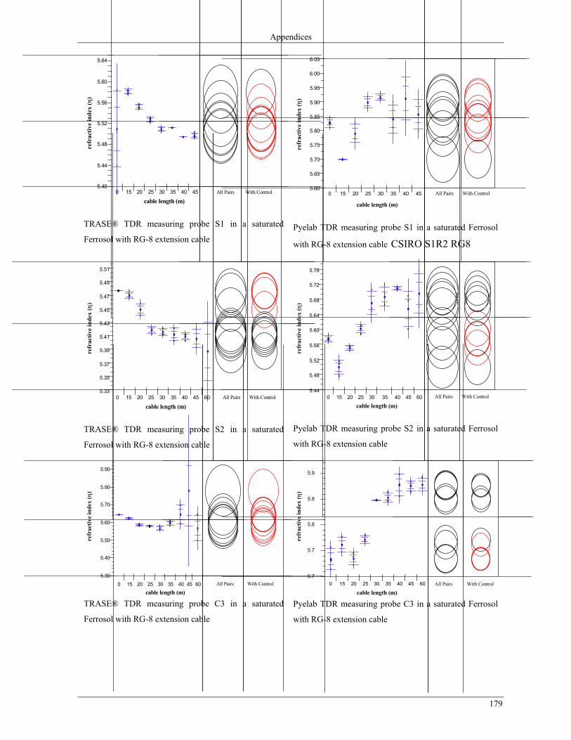
Appendices
179
5.40
5.44
5.48
5.52
5.56
5.60
5.64
0 15 20 25 30 35 40 45 All Pairs With Control
cable length (m)
refr
activ
e in
dex
(η)
TRASE® TDR measuring probe S1 in a saturated
Ferrosol with RG-8 extension cable
5.60
5.65
5.70
5.75
5.80
5.85
5.90
5.95
6.00
6.05
0 15 20 25 30 35 40 45 All Pairs With Control
refr
activ
e in
dex
(η)
cable length (m)
Pyelab TDR measuring probe S1 in a saturated Ferrosol
with RG-8 extension cable CSIRO S1R2 RG8
5.33
5.35
5.37
5.39
5.41
5.43
5.45
5.47
5.49
5.51
0 15 20 25 30 35 40 45 60 All Pairs With Control
refr
activ
e in
dex
(η)
cable length (m)
TRASE® TDR measuring probe S2 in a saturated
Ferrosol with RG-8 extension cable
5.44
5.48
5.52
5.56
5.60
5.64
5.68
5.72
5.76
0 15 20 25 30 35 40 45 60 All Pairs With Control
refr
activ
e in
dex
(η)
cable length (m)
Pyelab TDR measuring probe S2 in a saturated Ferrosol
with RG-8 extension cable
5.30
5.40
5.50
5.60
5.70
5.80
5.90
0 15 20 25 30 35 40 45 60 All Pairs With Control
refr
activ
e in
dex
(η)
cable length (m)
TRASE® TDR measuring probe C3 in a saturated
Ferrosol with RG-8 extension cable
All Pairs With Control
refr
activ
e in
dex
(η)
cable length (m)
5.7
5.7
5.8
5.8
5.9
0 15 20 25 30 35 40 45 60
Pyelab TDR measuring probe C3 in a saturated Ferrosol
with RG-8 extension cable

B.H. George – Measuring soil water content
180
2.54
2.59
2.64
2.69
2.74
2.79
0 15 20 25 30 35 40 45 All Pairs With Control
cable length (m)
refr
activ
e in
dex
(η)
TRASE® TDR measuring probe S1 in an air-dry
Ferrosol with RG-8 extension cable
2.42
2.47
2.52
2.57
2.62
2.67
2.72
0 15 20 25 30 35 40 45 60 All Pairs With Control
cable length (m)
refr
activ
e in
dex
(η)
Pyelab TDR measuring probe S1 in an air-dry Ferrosol
with RG-8 extension cable
2.48
2.50
2.52
2.54
2.56
2.58
2.60
0 15 20 25 30 35 40 45 All Pairs With Control
cable length (m)
refr
activ
e in
dex
(η)
TRASE® TDR measuring probe S2 in an air-dry
Ferrosol with RG-8 extension cable
2.55
2.60
2.65
2.70
2.75
0 15 20 25 30 35 40 45 60 All Pairs With Control
cable length (m)
refr
activ
e in
dex
(η)
Pyelab TDR measuring probe S2 in an air-dry Ferrosol
with RG-8 extension cable
2.19
2.21
2.23
2.25
2.27
2.29
2.31
0 15 20 25 All Pairs With Control
cable length (m)
refr
activ
e in
dex
(η)
TRASE® TDR measuring probe C3 in an air-dry
Ferrosol with RG-8 extension cable
2.05
2.10
2.15
2.20
2.25
2.30
2.35
0 15 20 25 30 35 40 45 60 All Pairs With Control
cable length (m)
refr
activ
e in
dex
(η)
Pyelab TDR measuring probe C3 in an air-dry Ferrosol
with RG-8 extension cable
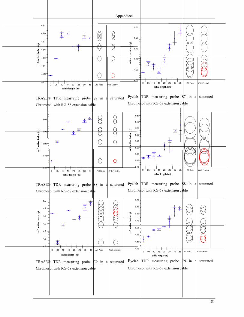
Appendices
181
4.77
4.79
4.81
4.83
4.85
4.87
4.89
4.91
0 05 10 15 20 25 30 35 All Pairs With Control
refr
activ
e in
dex
(η)
cable length (m)
TRASE® TDR measuring probe S7 in a saturated
Chromosol with RG-58 extension cable
4.80
4.90
5.00
5.10
5.20
5.30
0 05 10 15 20 25 30 35 All Pairs With Control
refr
activ
e in
dex
(η)
cable length (m)
Pyelab TDR measuring probe S7 in a saturated
Chromosol with RG-58 extension cable
4.84
4.89
4.94
4.99
5.04
0 05 10 15 20 25 30 35 All Pairs With Control
refr
activ
e in
dex
(η)
cable length (m)
TRASE® TDR measuring probe S8 in a saturated
Chromosol with RG-58 extension cable
5.00
5.10
5.20
5.30
5.40
5.50
5.60
5.70
5.80
0 05 10 15 20 25 30 35 All Pairs With Control
refr
activ
e in
dex
(η)
cable length (m)
Pyelab TDR measuring probe S8 in a saturated
Chromosol with RG-58 extension cable
4.8
4.8
4.9
4.9
4.9
4.9
5.0
0 05 10 15 20 25 30 35 All Pairs With Control
refr
activ
e in
dex
(η)
cable length (m) TRASE® TDR measuring probe C9 in a saturated
Chromosol with RG-58 extension cable
4.75
4.85
4.95
5.05
5.15
5.25
5.35
5.45
0 05 10 15 20 25 30 35 All Pairs With Control
refr
activ
e in
dex
(η)
cable length (m)
Pyelab TDR measuring probe C9 in a saturated
Chromosol with RG-58 extension cable

B.H. George – Measuring soil water content
182
2.00
2.10
2.20
2.30
2.40
0 5 10 15 20 25 30 35 All Pairs With Control
cable length (m)
refr
activ
e in
dex
(η)
Pyelab TDR measuring probe S7 in an air-dry Chromosol
with RG-58 extension
1.95
2.00
2.05
2.10
2.15
0 5 10 15 20 25 30 35 All Pairs With Control
cable length (m)
refr
activ
e in
dex
(η)
TRASE® TDR measuring probe S8 in an air-dry
Chromosol with RG-58 extension cable
1.95
2.00
2.05
2.10
2.15
2.20
2.25
2.30
2.35
0 5 10 15 20 25 30 35 All Pairs With Control
cable length (m)
refr
activ
e in
dex
(η)
Pyelab TDR measuring probe S8 in an air-dry Chromosol
with RG-58 extension cable
2.00
2.05
2.10
2.15
2.20
0 05 10 15 20 25 30 35 All Pairs With Control
cable length (m)
refr
activ
e in
dex
(η)
TRASE® TDR measuring probe C9 in an air-dry
Chromosol with RG-58 extension cable
2.00
2.05
2.10
2.15
2.20
2.25
2.30
2.35
0 05 10 15 20 25 30 35 All Pairs With Control
cable length (m)
refr
activ
e in
dex
(η)
Pyelab TDR measuring probe C9 in an air-dry Chromosol
with RG-58 extension cable

Appendices
183
4.71
4.73
4.75
4.77
4.79
4.81
4.83
0 15 20 25 30 35 40 45 60 All Pairs With Control
refr
activ
e in
dex
(η)
cable length (m)
TRASE® TDR measuring probe S7 in a saturated
Chromosol with RG-8 extension cable
4.79
4.89
4.99
5.09
5.19
5.29
0 15 20 25 30 35 40 45 60 All Pairs With Control
refr
activ
e in
dex
(η)
cable length (m)
Pyelab TDR measuring probe S7 in a saturated
Chromosol with RG-8 extension cable
4.85
4.87
4.89
4.91
4.93
4.95
0 15 20 25 30 35 40 45 60 All Pairs With Control
refr
activ
e in
dex
(η)
cable length (m)
TRASE® TDR measuring probe S8 in a saturated
Chromosol with RG-8 extension cable
5.00
5.10
5.20
5.30
5.40
5.50
5.60
5.70
5.80
5.90
0 15 20 25 30 35 40 45 60 All Pairs With Control
refr
activ
e in
dex
(η)
cable length (m)
Pyelab TDR measuring probe S8 in a saturated
Chromosol with RG-8 extension cable
4.80
4.85
4.90
4.95
5.00
0 15 20 25 30 35 40 60 All Pairs With Control
refr
activ
e in
dex
(η)
cable length (m) TRASE® TDR measuring probe C9 in a saturated
Chromosol with RG-8 extension cable
4.75
4.85
4.95
5.05
5.15
5.25
0 15 20 25 30 35 40 45 60 All Pairs With Control
refr
activ
e in
dex
(η)
cable length (m)
Pyelab TDR measuring probe C9 in a saturated
Chromosol with RG-8 extension cable

B.H. George – Measuring soil water content
184
1.96
1.98
2.00
2.02
2.04
2.06
2.08
2.10
2.12
0 15 20 30 35 40 45 All Pairs With Control
cable length (m)
refr
activ
e in
dex
(η)
TRASE® TDR measuring probe C7 in an air-dry
Chromosol with RG-8 extension
2.04
2.14
2.24
2.34
0 15 20 30 35 40 45 All Pairs With Control
cable length (m)
refr
activ
e in
dex
(η)
Pyelab TDR measuring probe C7 in an air-dry
Chromosol with RG-8 extension cable
1.95
1.97
1.99
2.01
2.03
2.05
2.07
2.09
0 15 20 25 30 35 40 45 All Pairs With Control
cable length (m)
refr
activ
e in
dex
(η)
TRASE® TDR measuring probe C8 in an air-dry
Chromosol with RG-8 extension cable
1.96
2.01
2.06
2.11
2.16
2.21
0 15 20 25 30 35 40 45 60 All Pairs With Control
cable length (m)
refr
activ
e in
dex
(η)
Pyelab TDR measuring probe S8 in an air-dry
Chromosol with RG-8 extension cable
2.00
2.02
2.04
2.06
2.08
2.10
0 15 20 25 30 35 40 All Pairs With Controlcable length (m)
refr
activ
e in
dex
(η)
TRASE® TDR measuring probe C9 in an air-dry
Chromosol with RG-8 extension cable
2.00
2.05
2.10
2.15
2.20
2.25
2.30
0 15 20 25 30 35 40 45 60 All Pairs With Controlcable length (m)
refr
activ
e in
dex
(η)
Pyelab TDR measuring probe C9 in an air-dry
Chromosol with RG-8 extension cable

Appendices
185
4.26
4.28
4.30
4.32
4.34
4.36
4.38
0 05 10 15 20 25 30 35 All Pairs With Control
refr
activ
e in
dex
(η)
cable length (m)
TRASE® TDR measuring probe S10 in a saturated sand
with RG-8 extension cable
3.96
4.00
4.04
4.08
4.12
4.16
0 05 10 15 20
Pyelab TDR measuring probe S10 in a saturated sand with
RG-58 extension cable
4.03
4.04
4.05
4.06
4.07
4.08
4.09
4.10
4.11
0 05 10 15 20 25 30 35 All Pairs With Control
refr
activ
e in
dex
(η)
cable length (m)
TRASE® TDR measuring probe C11 in a saturated sand
with RG-58 extension cable
3.94
3.99
4.04
4.09
4.14
4.19
0 05 10 15 20 25 30 35 All Pairs With Control
refr
activ
e in
dex
(η)
cable length (m)
Pyelab TDR measuring probe C11 in a saturated sand with
RG-58 extension cable
4.18
4.20
4.22
4.24
4.26
4.28
4.30
4.32
0 15 20 25 30 35 40 45 All Pairs With Control
refr
activ
e in
dex
(η)
cable length (m)
TRASE® TDR measuring probe S10 in a saturated sand
with RG-8 extension cable
4.05
4.10
4.15
4.20
4.25
4.30
4.35
0 15 20 30 All Pairs With Control
refr
activ
e in
dex
(η)
cable length (m)
Pyelab TDR measuring probe S10 in a saturated sand
with RG-8 extension cable
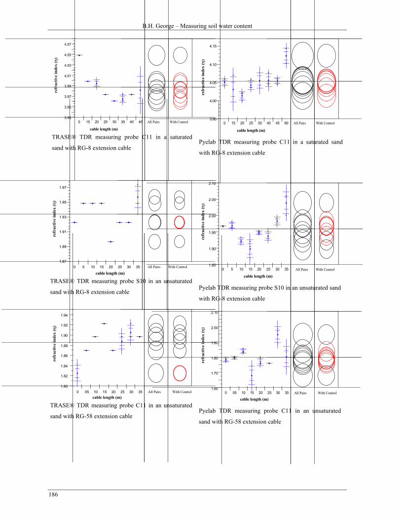
B.H. George – Measuring soil water content
186
3.93
3.95
3.97
3.99
4.01
4.03
4.05
4.07
0 15 20 25 30 35 40 45 All Pairs With Control
refr
activ
e in
dex
(η)
cable length (m)
TRASE® TDR measuring probe C11 in a saturated
sand with RG-8 extension cable
3.95
4.00
4.05
4.10
4.15
0 15 20 25 35 40 45 60 All Pairs With Control
refr
activ
e in
dex
(η)
cable length (m) Pyelab TDR measuring probe C11 in a saturated sand
with RG-8 extension cable
0 5 10 15 20 25 30 351.87
1.89
1.91
1.93
1.95
1.97
All Pairs With Control
cable length (m)
refr
activ
e in
dex
(η)
TRASE® TDR measuring probe S10 in an unsaturated
sand with RG-8 extension cable
1.85
1.90
1.95
2.00
2.05
2.10
0 5 10 15 20 25 30 35 All Pairs With Control
cable length (m)
refr
activ
e in
dex
(η)
Pyelab TDR measuring probe S10 in an unsaturated sand
with RG-8 extension cable
1.80
1.82
1.84
1.86
1.88
1.90
1.92
1.94
0 05 10 15 20 25 30 35 All Pairs With Controlcable length (m)
refr
activ
e in
dex
(η)
TRASE® TDR measuring probe C11 in an unsaturated
sand with RG-58 extension cable
1.60
1.70
1.80
1.90
2.00
2.10
0 05 10 15 20 25 30 35 All Pairs With Control
cable length (m)
refr
activ
e in
dex
(η)
Pyelab TDR measuring probe C11 in an unsaturated
sand with RG-58 extension cable

Appendices
187
1.84
1.86
1.88
1.90
1.92
1.94
0 15 20 25 30 35 40 All Pairs With Control
cable length (m)
refr
activ
e in
dex
(η)
TRASE® TDR measuring probe S10 in an air-dry sand
with RG-8 extension cable
1.80
1.90
2.00
0 15 20 25 30 35 40 45 60
1.95
1.85
All Pairs With Control
cable length (m)
refr
activ
e in
dex
(η)
Pyelab TDR measuring probe S10 in an air-dry sand
with RG-8 extension
1.76
1.78
1.80
1.82
1.84
1.86
0 15 20 25 30 35 40 45 All Pairs With Controlcable length (m)
refr
activ
e in
dex
(η)
TRASE® TDR measuring probe C11 in an sir-dry sand
with RG-8 extension cable
1.71
1.76
1.81
1.86
1.91
1.96
2.01
0 15 20 25 30 35 40 45 60 All Pairs With Controlcable length (m)
refr
activ
e in
dex
(η)
Pyelab TDR measuring probe C11 in an air-dry sand
with RG-8 extension

B.H. George – Measuring soil water content
188
Appendix 3-1
Distribution of the NMM counts in a sand drum and water drum representing the likely extreme
conditions of measurement with the NMM technology.
200
250
300
350
400
450
500
550
35000
35500
36000
36500
37000
37500
38000
38500
39000
300
350
400
450
500
36000
36250
36500
36750
37000
37250
37500
340
350
360
370
380
390
400
410
420
430
440
36300
36400
36500
36600
36700
36800
36900
37000
37100
37200

Appendices
189
350
360
370
380
390
400
410
420
430
36400
36500
36600
36700
36800
36900
37000
37100
375
380
385
390
395
400
405
410
415
36450
36500
36550
36600
36650
36700
36750
36800
36850
36900
Spread of NMM counts in a sand drum
at 1-second (over page top), 4-seconds,
16-seconds, 32-seconds (this page top)
and 64-seconds count time.
Spread of NMM counts in a water drum
at 1-second (over page top), 4-seconds,
16-seconds, 32-seconds (this page top)
and 64-seconds count time.

B.H. George – Measuring soil water content
190
Appendix 4-1
Calibration coefficients for the EnviroSCAN® FD system S0077 supplied with the instrument.
Sensor
depth (m)
Sensor 1
(air)
Sensor 1
(water)
Sensor 2
(air)
Sensor 2
(water)
0.1 48493 33123 49241 32734
0.2 49445 32867 48659 32246
0.3 48832 33259 49867 32930
0.4 50079 33657 49905 33873
0.5 49544 33317 49200 33424
0.7 48785 33371 49858 32802
0.9 48745 32927 49573 32847
1.2 50261 32809 49362 33085
The relationship used for the conversion of universal frequency (UF) to volumetric soil water
content (θ) for the EnviroSCAN® FD system is based on unpublished results of J.C. Dighton & P.J.
Dillon (CSIRO, Adelaide) from two soil types (unknown) where the UF = 0.3316 (± 0.0337) + θ ×
1.520665 (± 0.0611).
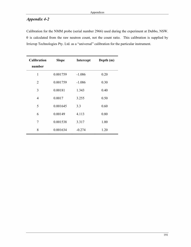
Appendices
191
Appendix 4-2
Calibration for the NMM probe (serial number 2966) used during the experiment at Dubbo, NSW.
θ is calculated from the raw neutron count, not the count ratio. This calibration is supplied by
Irricrop Technologies Pty. Ltd. as a “universal” calibration for the particular instrument.
Calibration
number
Slope Intercept Depth (m)
1 0.001759 -1.086 0.20
2 0.001759 -1.086 0.30
3 0.00181 1.343 0.40
4 0.0017 3.255 0.50
5 0.001645 3.3 0.60
6 0.00149 4.113 0.80
7 0.001538 3.317 1.00
8 0.001634 -0.274 1.20
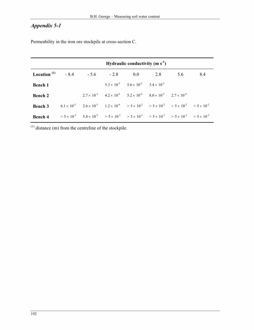
B.H. George – Measuring soil water content
192
Appendix 5-1
Permeability in the iron ore stockpile at cross-section C.
Hydraulic conductivity (m s-1)
Location (1) - 8.4 - 5.6 - 2.8 0.0 2.8 5.6 8.4
Bench 1 5.3 × 10⁻⁵ 5.6 × 10⁻⁵ 3.4 × 10⁻⁵
Bench 2 2.7 × 10⁻⁵ 4.2 × 10⁻⁶ 5.2 × 10⁻⁶ 8.0 × 10⁻⁵ 2.7 × 10⁻⁴
Bench 3 6.1 × 10⁻⁵ 2.6 × 10⁻⁵ 1.2 × 10⁻⁴ > 5 × 10⁻² > 5 × 10⁻² > 5 × 10⁻² > 5 × 10⁻²
Bench 4 > 5 × 10⁻² 5.4 × 10⁻⁵ > 5 × 10⁻² > 5 × 10⁻² > 5 × 10⁻² > 5 × 10⁻² > 5 × 10⁻²
(1) distance (m) from the centreline of the stockpile.