Embed Size (px)
Citation preview
A COMPARISON BETWEEN VIRTUAL CODE
MANAGEMENT TECHNIQUES
by
Joseph B. Manzano
A dissertation submitted to the Faculty of the University of Delaware in partialfulfillment of the requirements for the degree of Doctor of Philosophy in Electrical andComputer Engineering
Summer 2011
c© 2011 Joseph B. ManzanoAll Rights Reserved
A COMPARISON BETWEEN VIRTUAL CODE
MANAGEMENT TECHNIQUES
by
Joseph B. Manzano
Approved:Kenneth E. Barner, Ph.D.Chair of the Department of Electrical and Computer Engineering
Approved:Babatunde Ogunnaike, Ph.D.Interim Dean of the College of Engineering
Approved:Charles G. Riordan, Ph.D.Vice Provost for Graduate and Professional Education
I certify that I have read this dissertation and that in my opinion it meets theacademic and professional standard required by the University as a dissertation forthe degree of Doctor of Philosophy.
Signed:Guang R. Gao, Ph.D.Professor in charge of dissertation
I certify that I have read this dissertation and that in my opinion it meets theacademic and professional standard required by the University as a dissertation forthe degree of Doctor of Philosophy.
Signed:Xiaoming Li, Ph.D.Member of dissertation committee
I certify that I have read this dissertation and that in my opinion it meets theacademic and professional standard required by the University as a dissertation forthe degree of Doctor of Philosophy.
Signed:Hui Fang, Ph.D.Member of dissertation committee
I certify that I have read this dissertation and that in my opinion it meets theacademic and professional standard required by the University as a dissertation forthe degree of Doctor of Philosophy.
Signed:Andres Marquez, Ph.D.Member of dissertation committee

To my parents (real and imaginary) for all their support and understanding.
iv
ACKNOWLEDGEMENTS
As this journey ends, I would like to thank all the people that helped me during
these years. First, I would like to thank my family, my sisters, Carolina and Gaby; and my
parents for all their support and kind words during the years, and there have been many
years. Next, I will like to thank my best friends, Juergen Ributzka, Jean Christophe Beyler
and Eunjung Park for all their help and encouraging words during these years.
Next I would like to thank all the people in the CAPSL group for all the time and
patience that they have had with me over the many many years that I was there. This list
includes, but it is not limited to Fei Chen, Weirong Zhu, Yuan Zhang, Divya Parthasarathi,
Dimitrij Krepis, Daniel Orozco, Kelly Livingston, Chen Chen, Joshua Suetterlein, Sunil
Shrestha and Stephane Zuckerman. Thanks guys for several amazing years.
Finally, I want to thank my advisor, Dr Guang R. Gao and his wife, Peggy, for all
their advice and guidance over the years and of course their support. As this stage is ending,
I just want to let know the people in this list and many others, that you made this journey
fun, exciting and worth it. Thanks from the bottom of my heart to all of you.
God bless.
v
TABLE OF CONTENTS
LIST OF FIGURES . . . . . . . . . . . . . . . . . . . . . . . . . . . . . . . . . . . xLIST OF TABLES . . . . . . . . . . . . . . . . . . . . . . . . . . . . . . . . . . . . xivLIST OF SOURCE CODE FRAGMENTS . . . . . . . . . . . . . . . . . . . . xvABSTRACT . . . . . . . . . . . . . . . . . . . . . . . . . . . . . . . . . . . . . . . xvi
Chapter
1 INTRODUCTION . . . . . . . . . . . . . . . . . . . . . . . . . . . . . . . . . . 1
1.1 The Power Race and Multi Core Designs . . . . . . . . . . . . . . . . . . . . 4
1.1.1 The Pentium Family Line . . . . . . . . . . . . . . . . . . . . . . . . 51.1.2 The Multi Core Era: Selected Examples . . . . . . . . . . . . . . . . 121.1.3 Multi Core: IBM’s POWER6 and POWER7 Chips . . . . . . . . . . 121.1.4 Multi Core: Intel’s Core’s Family of Processors . . . . . . . . . . . . 141.1.5 Multi Core: Sun UltraSPARC T2 . . . . . . . . . . . . . . . . . . . . 151.1.6 Multi Core: The Cray XMT . . . . . . . . . . . . . . . . . . . . . . . 171.1.7 Many Core: The Tile64 . . . . . . . . . . . . . . . . . . . . . . . . . 191.1.8 Many Core: The Cyclops-64 . . . . . . . . . . . . . . . . . . . . . . . 21
1.2 Problem Formulation: an Overview . . . . . . . . . . . . . . . . . . . . . . . 241.3 Contributions . . . . . . . . . . . . . . . . . . . . . . . . . . . . . . . . . . . 24
2 PRODUCTIVITY STUDIES . . . . . . . . . . . . . . . . . . . . . . . . . . . 27
2.1 Atomic Sections: Overview . . . . . . . . . . . . . . . . . . . . . . . . . . . . 292.2 The Delaware Programmability, Productivity and Proficiency Inquiry: An
Overview . . . . . . . . . . . . . . . . . . . . . . . . . . . . . . . . . . . . . . 31
2.2.1 P3I Infrastructure and Procedures . . . . . . . . . . . . . . . . . . . . 342.2.2 The Web Survey: Purpose . . . . . . . . . . . . . . . . . . . . . . . . 372.2.3 P3I Results . . . . . . . . . . . . . . . . . . . . . . . . . . . . . . . . 382.2.4 P3I Version 2 . . . . . . . . . . . . . . . . . . . . . . . . . . . . . . . 39
vi
3 OPEN OPELL: AN OVERVIEW . . . . . . . . . . . . . . . . . . . . . . . . 48
3.1 The Cell Architecture . . . . . . . . . . . . . . . . . . . . . . . . . . . . . . . 48
3.1.1 The PowerPC Processing Element . . . . . . . . . . . . . . . . . . . . 503.1.2 The Synergistic Processing Element . . . . . . . . . . . . . . . . . . . 513.1.3 The Element Interconnect Bus . . . . . . . . . . . . . . . . . . . . . . 523.1.4 The Memory Subsystem and the Flex I/O Interface . . . . . . . . . . 52
3.2 Programming Models . . . . . . . . . . . . . . . . . . . . . . . . . . . . . . . 54
3.2.1 OpenOPELL and OpenMP . . . . . . . . . . . . . . . . . . . . . . . 54
3.2.1.1 Single Source Compilation . . . . . . . . . . . . . . . . . . . 593.2.1.2 Simple Execution Handler . . . . . . . . . . . . . . . . . . . 593.2.1.3 Software Cache . . . . . . . . . . . . . . . . . . . . . . . . . 613.2.1.4 Overlay / Partition Manager . . . . . . . . . . . . . . . . . 63
4 PARTITION MANAGER FRAMEWORK . . . . . . . . . . . . . . . . . . 67
4.1 Toolchain Modifications . . . . . . . . . . . . . . . . . . . . . . . . . . . . . 67
4.1.1 Compiler Changes . . . . . . . . . . . . . . . . . . . . . . . . . . . . 68
4.1.1.1 Command Line Flags . . . . . . . . . . . . . . . . . . . . . . 694.1.1.2 Pragma Directives . . . . . . . . . . . . . . . . . . . . . . . 694.1.1.3 Compiler Internals . . . . . . . . . . . . . . . . . . . . . . . 71
4.1.2 Assembler Changes . . . . . . . . . . . . . . . . . . . . . . . . . . . . 724.1.3 Linker Changes . . . . . . . . . . . . . . . . . . . . . . . . . . . . . . 754.1.4 Discussion and Future Work . . . . . . . . . . . . . . . . . . . . . . . 76
4.2 Partition Manager and Its Framework . . . . . . . . . . . . . . . . . . . . . . 78
4.2.1 Common Terminology . . . . . . . . . . . . . . . . . . . . . . . . . . 784.2.2 The Partition Manager . . . . . . . . . . . . . . . . . . . . . . . . . . 79
4.2.2.1 The Partition List . . . . . . . . . . . . . . . . . . . . . . . 794.2.2.2 The Partition Stack . . . . . . . . . . . . . . . . . . . . . . 814.2.2.3 The Partition Buffer . . . . . . . . . . . . . . . . . . . . . . 814.2.2.4 The Partition Manager Kernel . . . . . . . . . . . . . . . . 81
vii
4.2.2.5 The Anatomy of a Partitioned Call . . . . . . . . . . . . . . 82
4.2.3 Cell Implementation of the Partition Framework: Version 1 . . . . . . 83
4.2.3.1 Partition List Structures and Variables . . . . . . . . . . . . 834.2.3.2 Partition Stack Structures and Variables . . . . . . . . . . . 844.2.3.3 Partition Buffer Structures and Variables . . . . . . . . . . . 844.2.3.4 Partition Manager Support Structures, Variables and Calling
Procedure . . . . . . . . . . . . . . . . . . . . . . . . . . . . 85
4.2.4 A Partitioned Call on CBE: Version 1 . . . . . . . . . . . . . . . . . . 86
5 PARTITION MANAGER ENHANCEMENTS . . . . . . . . . . . . . . . . 90
5.1 The N Buffer: The Lazy Reuse Approaches . . . . . . . . . . . . . . . . . . . 90
5.1.1 The N Buffer Approach . . . . . . . . . . . . . . . . . . . . . . . . . 91
5.1.1.1 The Partition Buffer . . . . . . . . . . . . . . . . . . . . . . 915.1.1.2 The Partition Stack . . . . . . . . . . . . . . . . . . . . . . 925.1.1.3 The Modulus Method . . . . . . . . . . . . . . . . . . . . . 935.1.1.4 The LRU Method . . . . . . . . . . . . . . . . . . . . . . . 94
5.1.2 Cell Implementation of the Partition Framework: Version 2 . . . . . . 95
5.2 Partition Graph and Other Enhancements . . . . . . . . . . . . . . . . . . . 101
5.2.1 Victim Cache . . . . . . . . . . . . . . . . . . . . . . . . . . . . . . . 1015.2.2 Prefetching . . . . . . . . . . . . . . . . . . . . . . . . . . . . . . . . 1025.2.3 The Partition Graph . . . . . . . . . . . . . . . . . . . . . . . . . . . 103
5.2.3.1 Prefetching: Weighted Breadth First Fetch . . . . . . . . . . 105
5.2.4 Dynamic Code Enclaves . . . . . . . . . . . . . . . . . . . . . . . . . 105
6 EXPERIMENTAL TESTBED AND RESULTS . . . . . . . . . . . . . . . 107
6.1 Hardware Testbed . . . . . . . . . . . . . . . . . . . . . . . . . . . . . . . . . 1076.2 Software Testbed . . . . . . . . . . . . . . . . . . . . . . . . . . . . . . . . . 1076.3 Partition Manager Overhead . . . . . . . . . . . . . . . . . . . . . . . . . . . 1086.4 Partition Manager Policies and DMA Counts . . . . . . . . . . . . . . . . . . 109
viii
7 RELATED WORK . . . . . . . . . . . . . . . . . . . . . . . . . . . . . . . . . 113
7.1 A Historical Perspective . . . . . . . . . . . . . . . . . . . . . . . . . . . . . 113
7.1.1 The Embedded Field: Where Overlays Survived . . . . . . . . . . . . 1157.1.2 Data Movements in High Performance Computing . . . . . . . . . . . 115
7.2 Programmability for Cell B.E. . . . . . . . . . . . . . . . . . . . . . . . . . . 1167.3 Future Directions . . . . . . . . . . . . . . . . . . . . . . . . . . . . . . . . . 1177.4 Productivity Studies . . . . . . . . . . . . . . . . . . . . . . . . . . . . . . . 118
8 CONCLUSIONS . . . . . . . . . . . . . . . . . . . . . . . . . . . . . . . . . . . 119BIBLIOGRAPHY . . . . . . . . . . . . . . . . . . . . . . . . . . . . . . . . . . . . 120
ix
LIST OF FIGURES
1.1 1.1a Examples of Type two[62] and 1.1b Type one architectures[30] . . . . 3
1.2 Intel Processor frequency growth from 1973 to 2006 . . . . . . . . . . . . . 6
1.3 The Finite Automata for a simple Two Bit Saturation Scheme. Thanks toits symmetry spurious results will not destroy the prediction schema . . . . 8
1.4 The Finite Automata for the modified simple Two Bit Saturation Schemeused in the first Pentiums. Since it is not symmetric anymore the stronglytaken path will jump to strongly taken after one jump which will make thispath more prone to misprediction . . . . . . . . . . . . . . . . . . . . . . . 8
1.5 Two Level Branch Predictor . . . . . . . . . . . . . . . . . . . . . . . . . . 9
1.6 The Agree Predictor . . . . . . . . . . . . . . . . . . . . . . . . . . . . . . 10
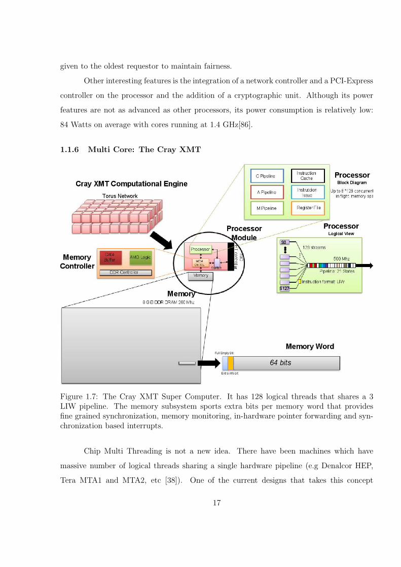
1.7 The Cray XMT Super Computer. It has 128 logical threads that shares a 3LIW pipeline. The memory subsystem sports extra bits per memory wordthat provides fine grained synchronization, memory monitoring, in-hardwarepointer forwarding and synchronization based interrupts. . . . . . . . . . . 17
1.8 A Logical diagram of the Cyclops-64 Architecture . . . . . . . . . . . . . . 22
2.1 A New Approach to Language Design. A new language should go throughseveral phases in its development to ensure that it has sound syntax andsemantics, it fits a specific demographic and it has a specific place in thefield. Moreover, optimization to the runtime libraries should be taken intoaccount while developing the language. . . . . . . . . . . . . . . . . . . . . 28
2.2 Atomic Section’s Syntax . . . . . . . . . . . . . . . . . . . . . . . . . . . . 31
2.3 Code Excerpt from Phase 0: A comparison between the lock implementation(left) and the AS implementation (right) for the unlucky banker . . . . . . 33
2.4 P3I Infrastructure . . . . . . . . . . . . . . . . . . . . . . . . . . . . . . . 34
x
2.5 P3I Infrastructure and Methodology . . . . . . . . . . . . . . . . . . . . . 36
2.6 Weight of each Participant . . . . . . . . . . . . . . . . . . . . . . . . . . . 38
2.7 Histogram of the Weights . . . . . . . . . . . . . . . . . . . . . . . . . . . 39
2.8 Weighted Average Time Data for Each Phase. In this case, there is a clearcorrelation between the reduction in time to correct solution from the lockexercises and the atomic sections. . . . . . . . . . . . . . . . . . . . . . . . 40
2.9 Activity Timeline for each participant in the study . . . . . . . . . . . . . 41
2.10 The phase’s percentage for each participant . . . . . . . . . . . . . . . . . 42
2.11 Total SLOC Average per Participant . . . . . . . . . . . . . . . . . . . . . 42
2.12 Total Average for SLOC . . . . . . . . . . . . . . . . . . . . . . . . . . . . 43
2.13 Total SLOC Average per Group . . . . . . . . . . . . . . . . . . . . . . . . 43
2.14 A comparison between the real and subjective weights . . . . . . . . . . . 44
2.15 An Absolute difference between the two difference types. The averagedifference is 0.12 and the standard deviation is 0.14 which represent verylow values . . . . . . . . . . . . . . . . . . . . . . . . . . . . . . . . . . . . 44
2.16 The total runtimes weighted by the low expertise formula . . . . . . . . . . 45
2.17 The total runtimes weighted by the normal expertise function . . . . . . . 45
2.18 The total runtimes weighted by the high expertise . . . . . . . . . . . . . . 46
3.1 Block Diagram of the Cell Broadband engine. This figure shows the blockdiagram of the Cell B.E. and its components (PPE and SPE). It also showsthe internal structures for the SPE pipelines and a high overview graph ofthe interconnect bus. . . . . . . . . . . . . . . . . . . . . . . . . . . . . . . 49
3.2 Allowed and forbidden OpenMP states. Any closed and encapsulatedfork-joins groups are allowed. This means that a child can never outlive itsparent and the lifetimes of threads cannot overlap between regions . . . . . 56
xi

3.3 High Level Overview of the Open OPELL framework. The micro kernel willtake of scheduling the jobs, the single source compiler will create the binaryfrom a single source tree, and the software cache and partition manager willtake to emulate the shared memory model required by OpenMP . . . . . . 58
3.4 A high level overview of the single source toolchain . . . . . . . . . . . . . 60
3.5 Components of the Simple Execution handler. It shows the shadow threadsrunning on the PPU side for each SPU and the communication channelsand flow between them. . . . . . . . . . . . . . . . . . . . . . . . . . . . . 62
3.6 Software Cache Merge Example Step 1: Before Write Back is Initialized . . 63
3.7 Software Cache Merge Example Step 2: Thread 2 succeed in the update.Thread 1 fails and tries again . . . . . . . . . . . . . . . . . . . . . . . . . 64
3.8 Software Cache Merge Example Step 3: Final State of the Memory Lineafter Thread 1 finished . . . . . . . . . . . . . . . . . . . . . . . . . . . . . 65
3.9 A high level overview of the Software cache structure . . . . . . . . . . . . 65
4.1 Toolchain Components and their respective roles . . . . . . . . . . . . . . 68
4.2 The format for a Partitioned Symbol . . . . . . . . . . . . . . . . . . . . . 76
4.3 The normal and enhanced binary image for the Partition Manager. TheTOE segment is a special segment used for the interaction between the PPEand SPE binaries. The CRT0 represents the entire C runtime code . . . . 77
4.4 A Partition Call showing all major partition manager components . . . . . 80
4.5 A Flowchart of the first section of the partition manager call. The logic flowof the initial section of the partition manager kernel. It checks if thepartition is loaded and if it is not, loaded and call the function . . . . . . 88
4.6 A Flowchart of the second section of the partition manager call. The logicflow of the return part of the partition manager kernel. It checks if thecallee partition still exists in memory, if it is not, load it. Return to thecaller afterwards. . . . . . . . . . . . . . . . . . . . . . . . . . . . . . . . . 89
5.1 Partition Manager Function Graph for the Modulus Example . . . . . . . 95
xii
5.2 States of each of the partition manager components across the function callsprovided by source code in listing 5.1 using the Modulus replacement policy 96
5.3 Partition Manager Function Graph for the LRU example . . . . . . . . . . 99
5.4 States of each of the partition manager components across the function callsprovided by source code in listing 5.2 using the LRU replacement policy . 100
5.5 Victim Cache Framework . . . . . . . . . . . . . . . . . . . . . . . . . . . 101
5.6 Prefetching Framework . . . . . . . . . . . . . . . . . . . . . . . . . . . . . 103
5.7 Creating a partition graph given a piece of source code . . . . . . . . . . . 104
6.1 DMA counts for all applications for an unoptimized one buffer, an optimizedone buffer, optimized two buffers and optimized four buffer versions . . . . 110
6.2 Cycle counts for all applications for an unoptimized one buffer, an optimizedone buffer, optimized two buffers and optimized four buffer versions . . . . 111
6.3 Ratio of Partition Manager calls versus DMA transfers . . . . . . . . . . . 112
6.4 LRU versus Modulus DMA counts for selected applications . . . . . . . . . 112
6.5 The victim cache comparison with LRU and Modulus policies . . . . . . . 112
xiii
LIST OF TABLES
4.1 Overview of New Assembly Directives . . . . . . . . . . . . . . . . . . . . 72
5.1 The Four States of a Partition . . . . . . . . . . . . . . . . . . . . . . . . . 92
6.1 Applications used in the Harahel testbed . . . . . . . . . . . . . . . . . . . 108
xiv
LIST OF SOURCE CODE FRAGMENTS
2.1 Atomic Section’s Example . . . . . . . . . . . . . . . . . . . . . . . . . . . . 30
3.1 OpenMP Example . . . . . . . . . . . . . . . . . . . . . . . . . . . . . . . . 54
3.2 MPI Example . . . . . . . . . . . . . . . . . . . . . . . . . . . . . . . . . . . 54
4.1 Pragma Directives Example . . . . . . . . . . . . . . . . . . . . . . . . . . . 70
4.2 Linker dump showing the preparation of the partition manager parameters . 73
4.3 Assembly File showing the partitioning directives . . . . . . . . . . . . . . . 74
4.4 A Partition Runtime Stack Node . . . . . . . . . . . . . . . . . . . . . . . . 84
5.1 Source code for the 2-buffer example . . . . . . . . . . . . . . . . . . . . . . 94
5.2 Source code for the 2-buffer example . . . . . . . . . . . . . . . . . . . . . . 98
xv
ABSTRACT
During the past decade (2000 to 2010) , the multi / many core architectures have seen
a renaissance, due to the insatiable appetite for performance. Limits on applications and
hardware technologies have put a stop to the frequency race in 2005. Current designs can be
divided into homogeneous and heterogeneous ones. Homogeneous designs are the easiest to
use since most toolchain components and system software do not need too much of a rewrite.
On the other end of the spectrum, there are the heterogeneous designs. These designs offer
tremendous computational raw power, but at the cost of losing hardware features that
might be necessary or even essential for certain types of system software and programming
languages. An example of this architectural design is the Cell B.E. processor which exhibits
both a heavy core and a group of simple cores designed to be its computational engine.
Recently, this architecture has been placed in the public eye thanks to being a central
component into one of the fastest super computers in the world. Moreover, it is the main
processing unit of the Sony’s Playstation 3 videogame console; the most powerful video
console currently in the market. Even though this architecture is very well known for its
accomplishments, it is also well known for its very low programmability. Due to this lack of
programmability, most of its system software efforts are dedicated to increase this feature.
Among the most famous ones are ALF, DaCS, CellSs, the single source XL compiler, the
IBM’s octopiler, among others. Most of these frameworks have been designed to support
(directly or indirectly) high level parallel programming languages. Among them, there is
an effort called Open OPELL from the University of Delaware. This toolchain / framework
tries to bring the OpenMP parallel programming model (De facto shared memory parallel
programming paradigm) to the Cell B.E. architecture. The OPELL framework is composed
of four components: a single source toolchain, a very light SPU kernel, a software cache and
a partition / code overlay manager. This extra layer increases the system’s programmability,
xvi
but it also increased the runtime system’s overhead. To reduce the overhead, each of the
components can be further optimized. This thesis concentrates on optimizing the partition
manager components by reducing the number of long latency transactions (DMA transfers)
that it produces. The contributions of this thesis are as following:
1. The development of a dynamic framework that loads and manages partitions across
function calls. In this manner, the restrictive memory problem can be alleviated and
the range of applications that can be run on the co-processing unit is expanded.
2. The implementation of replacement policies that are useful to reduce the number of
DMA transfers across partitions. Such replacement policies aim to optimize the most
costly operations in the proposed framework. Such replacements can be of the form
of buffer divisions, rules about eviction and loading, etc.
3. A quantification of such replacement policies given a selected set of applications and
a report of the overhead of such policies. Although several policies can be given, a
quantitative study is necessary to analyze which policy is best in which application
since the code can have different behaviors.
4. An API that can be easily ported and extended to several types of architectures.
The problem of restricted space is not going away. The new trend seems to favor an
increasing number of cores (with local memories) instead of more hardware features
and heavy system software. This means that frameworks like the one proposed in
this thesis will become more and more important as the wave of multi / many core
continues its ascent.
5. A productivity study that tries to define the elusive concept of productivity with a
set of metrics and the introduction of expertise as weighting functions.
Finally, the whole framework can be adapted to support task based frameworks, by
using the partition space as a task buffer and loading the code on demand with minimal
user interaction. This type of tasks are called Dynamic Code Enclaves or DyCE.
xvii
Chapter 1
INTRODUCTION
During the last decade, multi core and many core architectures have invaded all
aspects of computing. From embedded processors to high end servers and massive super-
computers, the multi / many core architectures have made their presence known. Their rise
is due to several factors; however, the most cited one is the phenomenon called “the power
wall.” This “wall” refers to the lack of effective cooling technologies to dissipate the heat
produced by higher and higher frequency chips[57]. Thus, the race for higher frequency was
abruptly stopped around 2006 with the “transformation” of the (single core) Pentium line
and the birth of the Core Duo family [51]. For the rest of this chapter, when referring to
the new designs, I will be using the term multi core to refer to both many and multi core
designs, unless otherwise stated.
Nowadays, the multi core architectures have evolved into a gamut of designs and
features. Broadly, this myriad of designs can be classified into two camps. The first one
is the “Type One” architectures which describes “heavy” cores1 glued together in a single
die. Designs in this family includes the AMD Opteron family and all the Intel Core Duo
line. The “Type Two” architectures refers to designs in which many “simple” cores2 are put
together in a single die. Most of today designs have an upper limit of eight with a projected
increased to twelve and sixteen in the next two years, with designs like Nehalem and Sandy
1 i.e. Cores which have many advance features such as branch prediction, speculativeexecution and out of order engines
2 i.e. Cores that have simple features such as in order execution, single pipelines, lackof hardware memory coherence and explicit memory hierarchies; however, they maypossess esoteric features to increase performance such as Processor in Memory, Full /Empty bits, Random memory allocators, etc
1
bridge from Intel and AMD’s twelve-core Magni-Cours chips (being introduced in late 2011
or early 2012) [5].
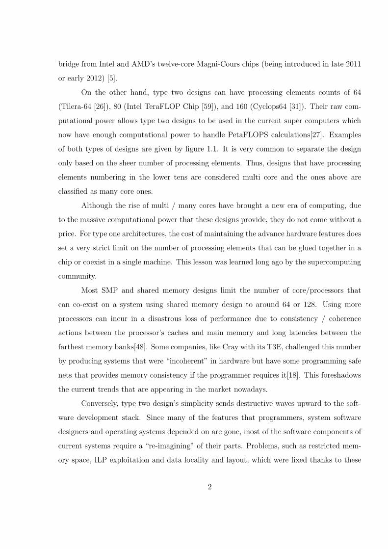
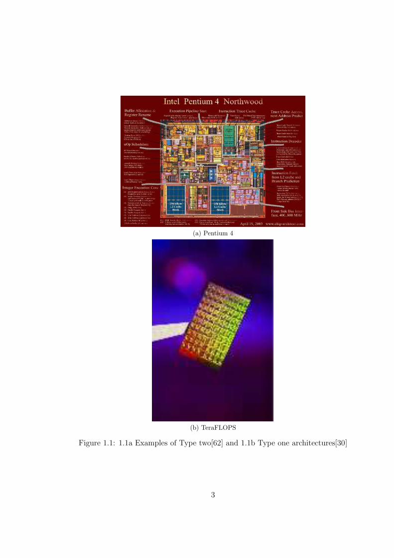
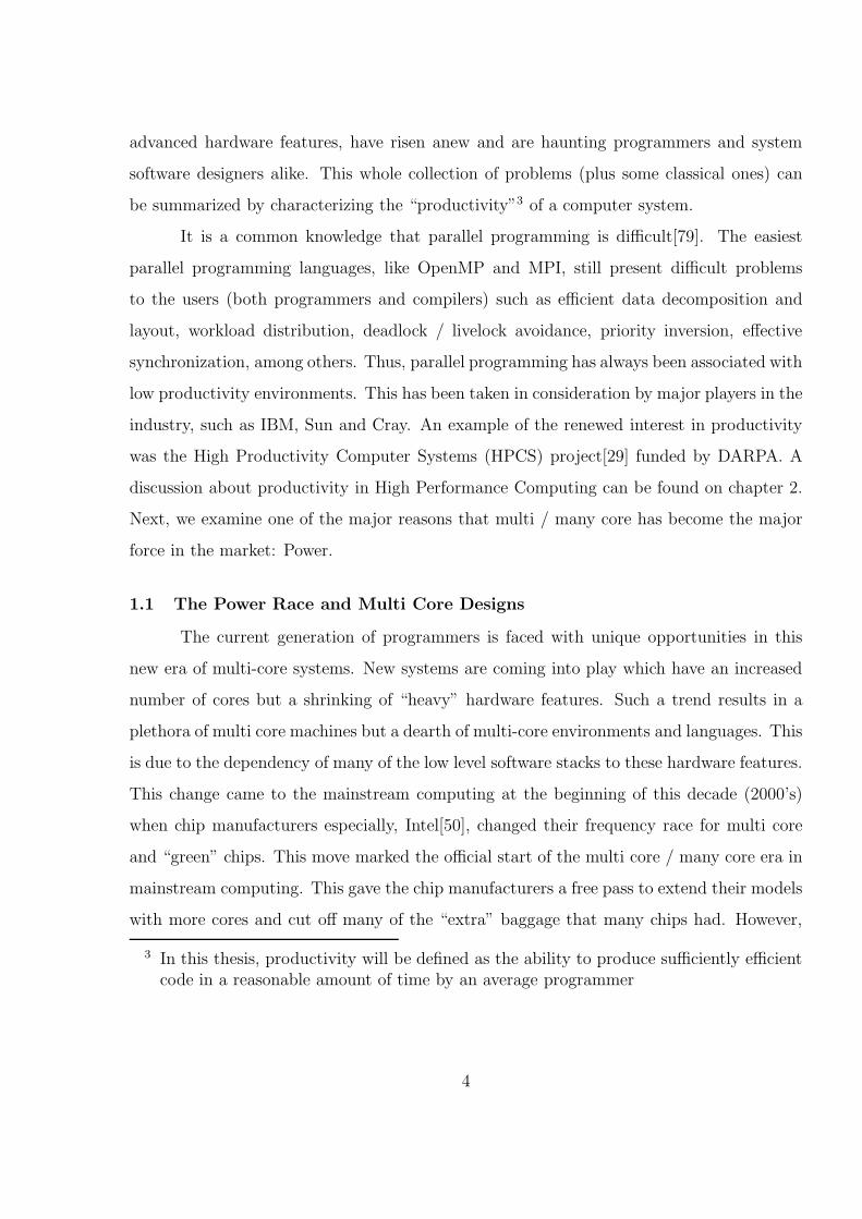
On the other hand, type two designs can have processing elements counts of 64
(Tilera-64 [26]), 80 (Intel TeraFLOP Chip [59]), and 160 (Cyclops64 [31]). Their raw com-
putational power allows type two designs to be used in the current super computers which
now have enough computational power to handle PetaFLOPS calculations[27]. Examples
of both types of designs are given by figure 1.1. It is very common to separate the design
only based on the sheer number of processing elements. Thus, designs that have processing
elements numbering in the lower tens are considered multi core and the ones above are
classified as many core ones.
Although the rise of multi / many cores have brought a new era of computing, due
to the massive computational power that these designs provide, they do not come without a
price. For type one architectures, the cost of maintaining the advance hardware features does
set a very strict limit on the number of processing elements that can be glued together in a
chip or coexist in a single machine. This lesson was learned long ago by the supercomputing
community.
Most SMP and shared memory designs limit the number of core/processors that
can co-exist on a system using shared memory design to around 64 or 128. Using more
processors can incur in a disastrous loss of performance due to consistency / coherence
actions between the processor’s caches and main memory and long latencies between the
farthest memory banks[48]. Some companies, like Cray with its T3E, challenged this number
by producing systems that were “incoherent” in hardware but have some programming safe
nets that provides memory consistency if the programmer requires it[18]. This foreshadows
the current trends that are appearing in the market nowadays.
Conversely, type two design’s simplicity sends destructive waves upward to the soft-
ware development stack. Since many of the features that programmers, system software
designers and operating systems depended on are gone, most of the software components of
current systems require a “re-imagining” of their parts. Problems, such as restricted mem-
ory space, ILP exploitation and data locality and layout, which were fixed thanks to these
2
(a) Pentium 4
(b) TeraFLOPS
Figure 1.1: 1.1a Examples of Type two[62] and 1.1b Type one architectures[30]
3
advanced hardware features, have risen anew and are haunting programmers and system
software designers alike. This whole collection of problems (plus some classical ones) can
be summarized by characterizing the “productivity”3 of a computer system.
It is a common knowledge that parallel programming is difficult[79]. The easiest
parallel programming languages, like OpenMP and MPI, still present difficult problems
to the users (both programmers and compilers) such as efficient data decomposition and
layout, workload distribution, deadlock / livelock avoidance, priority inversion, effective
synchronization, among others. Thus, parallel programming has always been associated with
low productivity environments. This has been taken in consideration by major players in the
industry, such as IBM, Sun and Cray. An example of the renewed interest in productivity
was the High Productivity Computer Systems (HPCS) project[29] funded by DARPA. A
discussion about productivity in High Performance Computing can be found on chapter 2.
Next, we examine one of the major reasons that multi / many core has become the major
force in the market: Power.
1.1 The Power Race and Multi Core Designs
The current generation of programmers is faced with unique opportunities in this
new era of multi-core systems. New systems are coming into play which have an increased
number of cores but a shrinking of “heavy” hardware features. Such a trend results in a
plethora of multi core machines but a dearth of multi-core environments and languages. This
is due to the dependency of many of the low level software stacks to these hardware features.
This change came to the mainstream computing at the beginning of this decade (2000’s)
when chip manufacturers especially, Intel[50], changed their frequency race for multi core
and “green” chips. This move marked the official start of the multi core / many core era in
mainstream computing. This gave the chip manufacturers a free pass to extend their models
with more cores and cut off many of the “extra” baggage that many chips had. However,
3 In this thesis, productivity will be defined as the ability to produce sufficiently efficientcode in a reasonable amount of time by an average programmer
4
this also involved a change on the way that main stream computing defines concepts such
as productivity[37].
As any computer engineer knows, the concept of productivity seems to be a very fluid
one. On one hand, we have performance being represented as code size, memory footprint
and power utilization (lower is better). Peak performance is still important but it can take a
second place when dealing with real time systems, in which a loss in performance is accept-
able as long as the quantum interval is respected. On the other hand, High Performance
Computing (HPC) plays a completely different game. On these systems, the total number
of Floating Point operations per second (FLOPS) is king. These systems and the applica-
tions written for them are created to exploit the most of the current technology to reach
the next computational barrier. As of the writing of this thesis, this barrier stands on the
PetaFLOPS (1015) range and there are many proposals to reach the next one (Exa) in the
not-so-distant future [78]. However, HPC, in particular, and the rest of the computing field
are changing. In HPC, and the general purpose field, another metric is being added: power.
Power was one of the major factors that put the nail in the coffin of the Pentium-4 line. To
gain a bit of perspective, we should take a view at features that made the Pentium-4 such
a power-hungry platform.
1.1.1 The Pentium Family Line
One of the perfect examples of the power trend is the Intel family of microprocessors.
The first Pentium microprocessors represented a jump in the general purpose processors.
They offered advance features such as SuperScalar designs4, 64 bit external databus, an
improved floating units, among others. However, this also started the famous frequency
race in which all major manufactures participated. In the case of Intel, all the iterations of
their Pentium family show an almost exponential increase on frequency from its introduction
in 1993 to 2006, as represented in figure 1.2. The Pentium line spanned three generations
of hardware design. These are the P5, the P6 and the Netburst architecture. The evolution
on these designs was represented by the addition of several features to increase single thread
4 Dynamic multiple issue techniques using principles presented in [80]
5
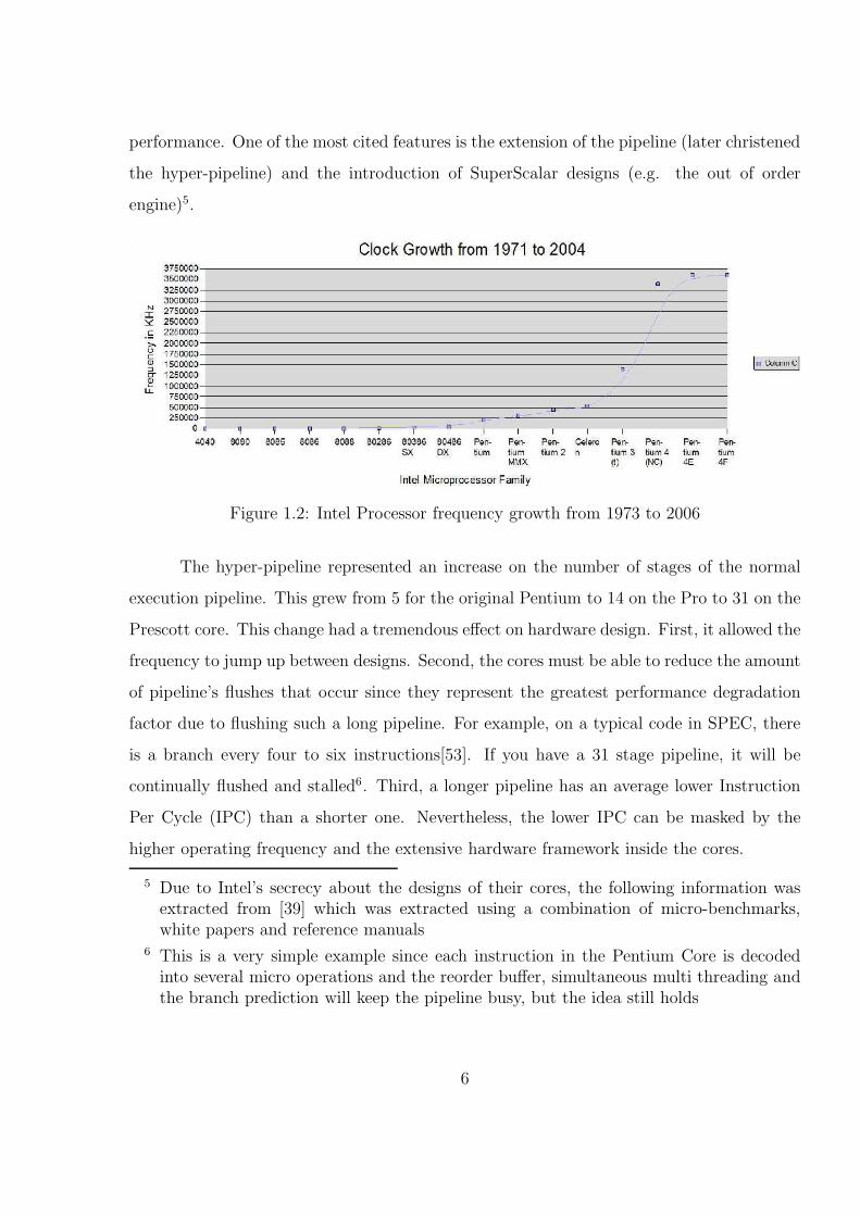
performance. One of the most cited features is the extension of the pipeline (later christened
the hyper-pipeline) and the introduction of SuperScalar designs (e.g. the out of order
engine)5.
Figure 1.2: Intel Processor frequency growth from 1973 to 2006
The hyper-pipeline represented an increase on the number of stages of the normal
execution pipeline. This grew from 5 for the original Pentium to 14 on the Pro to 31 on the
Prescott core. This change had a tremendous effect on hardware design. First, it allowed the
frequency to jump up between designs. Second, the cores must be able to reduce the amount
of pipeline’s flushes that occur since they represent the greatest performance degradation
factor due to flushing such a long pipeline. For example, on a typical code in SPEC, there
is a branch every four to six instructions[53]. If you have a 31 stage pipeline, it will be
continually flushed and stalled6. Third, a longer pipeline has an average lower Instruction
Per Cycle (IPC) than a shorter one. Nevertheless, the lower IPC can be masked by the
higher operating frequency and the extensive hardware framework inside the cores.
5 Due to Intel’s secrecy about the designs of their cores, the following information wasextracted from [39] which was extracted using a combination of micro-benchmarks,white papers and reference manuals
6 This is a very simple example since each instruction in the Pentium Core is decodedinto several micro operations and the reorder buffer, simultaneous multi threading andthe branch prediction will keep the pipeline busy, but the idea still holds
6
Due to the branch cost, Intel engineers dedicated a great amount of effort to cre-
ate very efficient Branch predictor schemes which alleviate the branch costs. Some basic
concepts need to be explained. When dealing with predicting a branch, two specific pieces
of information need to be known: do we need to jump and where to jump to. On the
Intel architecture (even in the new ones), the second question is answered by a hardware
structure called the Branch Target Buffer. This buffer is designed to keep all the targets
for all recently taken branches. In other words, it is a cache for branch targets. The answer
for the former question (i.e. do we need to jump) is a bit more complex to explain 7.
The Pentium family of processors can be seen as an example of the evolution of
branch prediction schemes. Every chips in this family have two sets of predictors. One is
the static predictor which enters in effect when no information about the branch is available
(i.e. the first time that is encountered). In this case, the predictor is very simple and it
predicts only based on the direction of the branch (i.e. forward branches are not taken
and backward branches are taken). If a branch has been logged into the branch prediction
hardware, then the dynamic prediction part of the framework takes effect. This dynamic
prediction differs greatly across members of this processor family.
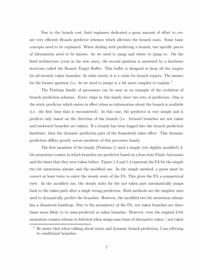
The first members of the family (Pentium 1) used a simple (yet slightly modified) 2-
bit saturation counter in which branches are predicted based on a four state Finite Automata
and the times that they were taken before. Figure 1.3 and 1.4 represent the FA for the simple
two bit saturation scheme and the modified one. In the simple method, a guess must be
correct at least twice to enter the steady state of the FA. This gives the FA a symmetrical
view. In the modified one, the steady state for the not taken part automatically jumps
back to the taken path after a single wrong prediction. Both methods are the simplest ones
used to dynamically predict the branches. However, the modified two bit saturation scheme
has a disastrous handicap. Due to the asymmetry of the FA, not taken branches are three
times more likely to be miss-predicted as taken branches. However, even the original 2-bit
saturation counter scheme is defeated when using some form of alternative taken / not taken
7 Be aware that when talking about static and dynamic branch prediction, I am referringto conditional branches
7
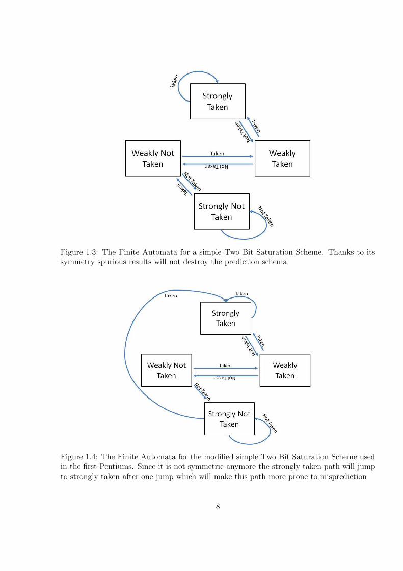
Figure 1.3: The Finite Automata for a simple Two Bit Saturation Scheme. Thanks to itssymmetry spurious results will not destroy the prediction schema
Figure 1.4: The Finite Automata for the modified simple Two Bit Saturation Scheme usedin the first Pentiums. Since it is not symmetric anymore the strongly taken path will jumpto strongly taken after one jump which will make this path more prone to misprediction
8
branch[3]. Because of this, the next members of the family (the MMX, Pro, Pentium 2 and
Pentium 3) used a two level adaptive predictor. Figure 1.5 shows a high overview of the
predictor and their respective components. This predictor was first proposed in [92]. The
main idea is that each branch has a branch history which keeps its occurrences n times in
the past. When a branch is predicted the history is checked and used to select one of several
saturation counters in a table called the Pattern history table. This table has 2n entries,
each of which contains a two-bit saturation counter. In this way, each of the counters learns
about their own n-bit pattern. A recurrent sequence of taken / not taken behavior for a
given branch is correctly predicted after a short learning process.
Figure 1.5: Two Level Branch Predictor
A major disadvantage of this method is the size of the Pattern history table which
grows exponentially with respect to the history bits n for each branch. This was solved
by making the Pattern history table and the branch history register shared across all the
branches. However, this added a new indexing function and the possibility of interference
9
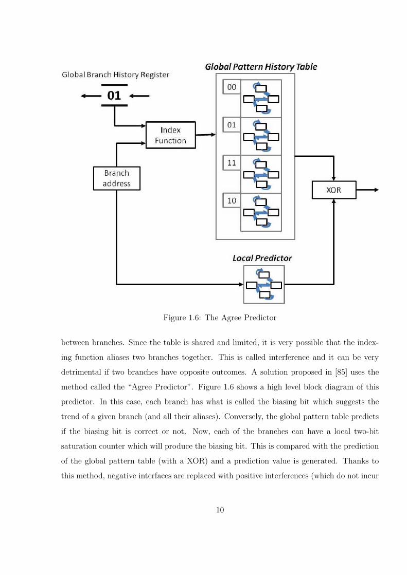
Figure 1.6: The Agree Predictor
between branches. Since the table is shared and limited, it is very possible that the index-
ing function aliases two branches together. This is called interference and it can be very
detrimental if two branches have opposite outcomes. A solution proposed in [85] uses the
method called the “Agree Predictor”. Figure 1.6 shows a high level block diagram of this
predictor. In this case, each branch has what is called the biasing bit which suggests the
trend of a given branch (and all their aliases). Conversely, the global pattern table predicts
if the biasing bit is correct or not. Now, each of the branches can have a local two-bit
saturation counter which will produce the biasing bit. This is compared with the prediction
of the global pattern table (with a XOR) and a prediction value is generated. Thanks to
this method, negative interfaces are replaced with positive interferences (which do not incur
10
any penalty).
Another important part of the pipeline is the addition of the Out of Order engine.
Out of order engines are used to schedule several concurrent instructions to distinct pipelines
without respecting a “strict” program order. However, all hazards (data, control and struc-
tural) are respected to ensure the correct execution of a given program. The out of order
engine accomplishes this by register renaming (called the Register Allocation Table (RAT),
multiple pipelines, reservation stations and a structure called the ReOrder Buffer (ROB).
During the first stage of the Pentium pipeline, the instructions are further translated into
the micro-operations (or uops for short). The decoding method is pretty much the same for
all of the Pentium family except on the number of decoding units and the function of each.
After the decoding is completed the uops go to the RAT and be renamed with temporary
registers. During the next step, the uops reserves an entry on the ROB and any available
operands are copied to the structure if available. Input registers in this case can fall into
three categories: the ones in which the inputs are in the permanent registers, the ones that
have the value in a ROB entry; and the ones in which the value is not ready yet. Next, the
“ready” uops are selected to go through the reservation stations and the execution ports for
each of the execution units. A ready uop is one which has all their dependencies resolved.
After the uops have been executed they enter a stage called retirement in which temporary
registers are written back to permanent registers and uops are retired from the ROB in
order. Besides these nominal stages, there are stages which take care of the prediction and
speculation (as described above) and some stages that are just designed to pass the data
from one part of the pipeline to another[77].
The out of order engine and the hyper-pipeline were introduced in the Pentium line
starting with Pentium Pro onward. The first Pentium design lacked the out of order engine.
Instead, it used the concept of instruction pairing to feed its two pipelines (named u and
v) which was mostly done by the programmer / toolchain. The differences between the
pipelines and the out of order engines of the subsequent generations were mostly on the
number and size of these features. The increase of the pipeline’s length (together with
the abilities of the ALU to “multiply” their frequencies for certain instructions) allowed
11
an unprecedented increase in performance during the Pentium line lifetime. However, this
came with the price of harder hits on the branches miss predictions, an increase on the
thermal and power requirements and an overall reduction of performance per watt [87].
Intel and AMD define the Thermal Design Power (TDP) metric to address the max-
imum amount of power, when running non-synthetic benchmarks, that the cooling system
needs to dissipate. During 2006, the TDP of selected chips (like the Pressler XE Pentium 4’s
flavor) reached as high as 130 watts[22]. As a side note, the most power hungry component
of a typical computer is not the CPU but the graphic card with maximum power usage (not
TDP) of 286 watts (for ATI Radeon HD 4870 X2 [20]). During that year, Intel abandoned
their frequency race and their Netburst architecture to a more streamlined architecture and
multiple cores8.
1.1.2 The Multi Core Era: Selected Examples
As the 2000s decade came to a close, the hardware designs got simpler and more
streamlined. Pipelines became shorter, reorder engines got smaller, and complex cores began
to recede to allow simpler (albeit more numerous) ones. Moreover, advances in fabrication
technology allowed smaller gates to be created and more components to be crammed inside
a chip. In the current generation, chips with 45 nm gate sizes are common and new chips
with 32 nm were introduced in early 2011[23]. In the current market, Multi core chips are
on the range of two to sixteen, rarely venturing into the thirty two range. On the other
hand, many core designs start at around 40 cores and grows upward from there[25]. In these
designs, the cores are much simpler. Several examples for both classifications are presented
below.
1.1.3 Multi Core: IBM’s POWER6 and POWER7 Chips
IBM, especially with its POWER series, has been in the multi core arena for a long
time. Due to that its main selling factor is servers (which require a high amount of through
8 The Pentium D represented the last hooray of the Netburst architecture in which itmarried the Netburst and multiple core design. However, it still had the power andheat problems exhibit by its ancestors.
12
put), IBM developed processors which have several cores to handle multiple requests. Their
chips have standard features such as dual cores and two-way Simultaneous Multi Threading,
for a total of four logical threads per processor. Larger core counts are created by using the
Multi-Chip Module packing technology to “fake” four and eight designs. Similar techniques
were used in the early days of the Intel’s Core chip family [39].
Up to the POWER5+, IBM continued with the trend of heavier chips with a plethora
of (very power hungry) hardware features and long pipelines. The POWER5 was notorious
for its 23 stages pipeline, out of order engine, register renaming and its power consumption.
Running from 2 GHz to 3 GHz, it wasn’t the speed demon that was expected. After
major revisions on the design, the next generation (POWER6) was born with the following
features: a higher frequency, an (almost) exclusion of the out of order engine, a reduction of
the pipeline stages from 23 to 13 and more streamlined pipeline stages. Major changes to the
design also included several components running at half or a fraction of the processor core
frequency (e.g. caches runs at half the frequency), a simplification of the branch prediction
hardware (from 3 BHT to one and a simplified scheme) and an increase on cache size by a
factor of 4. Even though the power profile of the POWER5 and POWER6 are practically
the same, the frequency of the POWER6 chips can be twice of their POWER5 counterparts
(up to 5 GHz). Details about both designs can be seen in [83] and [64].
For the next generation of POWER chips, IBM plans to create a design that is
concentrated on increasing the number of threads per processor. The POWER7 line consists
of dual, quad and octo cores. Each of them is capable of 4-way simultaneous multithreaded.
This achieves 32 logical threads in a single processor. Moreover, this chip has an aggressive
out of order engine and 32 MiB L3 cache of embedded DRAM. The pipelines in each core
runs with a reduced frequency compared to POWER6 ones (from 4.7 GHz in POWER6 to
4.14 GHz in POWER7). Several extra features include the dynamic change of frequency
and selectively switching on and off cores based on workload [84].
13
1.1.4 Multi Core: Intel’s Core’s Family of Processors
After the Netburst design was abandoned, Intel took a gander at the Pentium-M line
(their low power mobile processors) and re-designed them for multi-core. This was the birth
of the Core family of processors. These processors are marked by a reduction of the pipeline
lengths (from 31 to 14 on the first generation Cores) with an understandable decrease in
frequency, a simpler branch prediction and no (on almost all models) Hyper Threading.
However, they kept the out of order engine, continued using its Intel SpeedStep power (a
feature in which frequency decreases or increases according to workload) technology and
they have provided distributed and distinct Level 1 caches but shared Level 2 ones.
The first lines of processors in this family are the Core Solo and Duo cores. Introduced
in 2006, they are based on the Pentium M design and they have a very low Thermal Design
Power; anywhere from 9 to 31 watts and frequency ranging from 1.06 GHz to 2.33 GHz.
The only difference between the two processor’s flavors is the number of actual cores being
used. The Core duo supports two cores and the Solo only one. When using the Solo design
one of the cores is disabled; otherwise, the designs are identical. Some disadvantages of
this first generation include only 32-bit architecture support; a slight degradation for single
thread application and floating point; and higher memory latency than its contemporary
processors.
The next product in the line was the Core 2. These processors came into dual and
quad core and have several improvements over the Core line. It enhanced the pipeline to
handle four uops per cycles (in contrast to the 3 for the Core one)9 and the execution units
have been expanded from 64 to 128 bits. It also has native support for 64-bit and support
for the SSE3 instruction set. The Thermal Power Design for these chips ranged from 10
watts to 150 watts with frequencies ranging from 1.8 GHz to 3.2 GHz. It is important to
note that even though the upper limits of the Core 2 line (codenamed Kentfield Extreme
Edition) has a higher TDP as the most power hungry Pentium 4, we are talking about quad
cores (each capable of 2 virtual threads) instead of single ones. One of the major bottlenecks
9 However, the four instructions are not arbitrary, they have to be of a specific type tobe decoded at the same time.
14
of this design was that all the cores shared a single bus interconnect [39].
The next Intel line is the Core i7 processor (together with Core i3 and Core i5).
These chips are based on the Nehalem architecture. Nehalem architecture’s major change
is the replacement of the front side bus with a point-to-point network (christened Intel
QuickPath10) which has better scalability properties than the serializing bus, the integration
of the DRAM controller on the processor and the return of HyperThreading to the Intel
main line processors11. Other new features are an increase on the number of parallel uops
that can be executed concurrently, i.e. 128 uops in flight; a new second level predictor
for branches; the addition of a shared Level 3 cache; and the introduction of the SSE4.2
instruction set[39].
Besides the extensions and enhancements done to the cores, the chip power features
are worth a look too. Besides the Intel SpeedStep (i.e. Clock gating), the new Nehalem
designs have the TurboBoost Mode. Under this mode, under-utilized core are turned off
and their work re-distributed to other cores in the processor. The other cores on the chip
get a frequency boost to compensate for the extra work. This frequency boost continues
until the TDP of the machine is reached. Currently, the Nehalem design supports 4 and
8 cores natively (in contrast to the Core 2 Quad which used two Dual-core processor in a
single Multi Chip Module (MCM)).
1.1.5 Multi Core: Sun UltraSPARC T2
Sun Microsystems are well known on the server markets for their Chip Multithreaded
(CMTs). The latest one was the UltraSPARC T2 which concentrates on the idea of Simul-
taneous Multi threading (SMT). In these types of chips, Thread Level Parallelism (TLP)
is considered to be a major factor for performance instead of Instruction Level Parallelism
(ILP). This trend is reflected in their chip designs. The UltraSPARC T1 and T2 lack
complex out of order engines in favor of resource duplication for zero-cycle-context-switch
10 Long overdue, AMD has their Hyper Transport point-to-point interconnect introducedin their OPTERON line around 2003
11 It is true that HT was available during the Core era before this. However, the chipsthat used it were very high end chips reserved for gamers, HPC or computer experts
15
between logical threads. This allows the integrations of numerous cores and logical threads
on a single die. The UltraSPARC T1 had support for 32 logical threads running on 8 hard-
ware cores. The T2 increased the number of logical threads from 32 to 64. In a nutshell, an
UltraSPARC T2 chip has eight physical SPARC cores which contain two integer pipelines,
one floating point pipeline and one memory pipeline. Each of them capable of eight logical
threads; a shared 4 MiB Level 2 cache with 16-way associative and four dual channel Fully
Buffered DIMM (FBDIMM) memory controllers. Another major improvement is the inte-
gration of the floating point pipeline into the core and the doubling of the execution units
per core. An extra pipeline stage (called pick) is added to the core so that instructions from
its two threads can be executed every clock cycle. Even with the integration of the floating
point unit and the addition of the new stage, the number of pipeline stages is still below
other cores in this list: eight for the integer data path and 12 for the floating point path.
During execution, the logical threads are statically assigned to one of two groups. This
means that during the Fetch stage, any instruction from the 8 threads may be chosen (only
one instruction per cycle because the I-cache has only one port). However, after they are
assigned to a thread group, a single instruction from each group is chosen per cycle for ex-
ecution. This process happens on the Pick state of the pipeline. The SPARC core supports
a limited amount of speculation and it comes into three flavors: load speculation, condi-
tional branch and floating point traps. Speculated loads are assumed to be level 1 cache
hits. Speculated conditional branches are assumed to be non-taken. Finally, the Floating
point pipeline will speculate the trap for speculated floating point operations. Since a failed
speculated operation will cause a flush of the pipeline, each thread on the core keeps track
of their speculated instructions[86].
All the cores in the processor communicate with the eight banks of the 4 MiB Level 2
cache and the I/O by an 8 by 9 crossbar. The total bandwidth for writes in the crossbar is 90
GB / sec and for reads is 180 GB / sec. Since each port is distinct for each core and the paths
from the cores to the cache and vice versa are separate, there can be sixteen simultaneous
requests between the cores and the caches; eight load and /or store requests and eight data
returns, acknowledgments and / or invalidations. When arbitration is needed, priority is
16
given to the oldest requestor to maintain fairness.
Other interesting features is the integration of a network controller and a PCI-Express
controller on the processor and the addition of a cryptographic unit. Although its power
features are not as advanced as other processors, its power consumption is relatively low:
84 Watts on average with cores running at 1.4 GHz[86].
1.1.6 Multi Core: The Cray XMT
Figure 1.7: The Cray XMT Super Computer. It has 128 logical threads that shares a 3LIW pipeline. The memory subsystem sports extra bits per memory word that providesfine grained synchronization, memory monitoring, in-hardware pointer forwarding and syn-chronization based interrupts.
Chip Multi Threading is not a new idea. There have been machines which have
massive number of logical threads sharing a single hardware pipeline (e.g Denalcor HEP,
Tera MTA1 and MTA2, etc [38]). One of the current designs that takes this concept
17
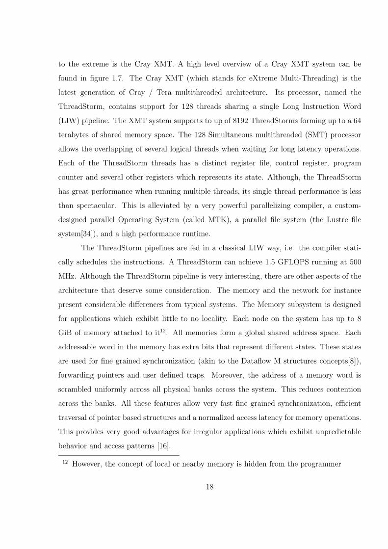
to the extreme is the Cray XMT. A high level overview of a Cray XMT system can be
found in figure 1.7. The Cray XMT (which stands for eXtreme Multi-Threading) is the
latest generation of Cray / Tera multithreaded architecture. Its processor, named the
ThreadStorm, contains support for 128 threads sharing a single Long Instruction Word
(LIW) pipeline. The XMT system supports to up of 8192 ThreadStorms forming up to a 64
terabytes of shared memory space. The 128 Simultaneous multithreaded (SMT) processor
allows the overlapping of several logical threads when waiting for long latency operations.
Each of the ThreadStorm threads has a distinct register file, control register, program
counter and several other registers which represents its state. Although, the ThreadStorm
has great performance when running multiple threads, its single thread performance is less
than spectacular. This is alleviated by a very powerful parallelizing compiler, a custom-
designed parallel Operating System (called MTK), a parallel file system (the Lustre file
system[34]), and a high performance runtime.
The ThreadStorm pipelines are fed in a classical LIW way, i.e. the compiler stati-
cally schedules the instructions. A ThreadStorm can achieve 1.5 GFLOPS running at 500
MHz. Although the ThreadStorm pipeline is very interesting, there are other aspects of the
architecture that deserve some consideration. The memory and the network for instance
present considerable differences from typical systems. The Memory subsystem is designed
for applications which exhibit little to no locality. Each node on the system has up to 8
GiB of memory attached to it12. All memories form a global shared address space. Each
addressable word in the memory has extra bits that represent different states. These states
are used for fine grained synchronization (akin to the Dataflow M structures concepts[8]),
forwarding pointers and user defined traps. Moreover, the address of a memory word is
scrambled uniformly across all physical banks across the system. This reduces contention
across the banks. All these features allow very fast fine grained synchronization, efficient
traversal of pointer based structures and a normalized access latency for memory operations.
This provides very good advantages for irregular applications which exhibit unpredictable
behavior and access patterns [16].
12 However, the concept of local or nearby memory is hidden from the programmer
18
The nodes of the Cray XMT are based on the boards for the Cray XT4 and XT5.
They are using AMD’s Torrenza Open Socket technologies and the same supporting infras-
tructure used for the XT machines. The nodes are arranged as a 3D torus connected using
the proprietary Cray SeaStar2 network. This switch sports an embedded PowerPC which
manages two DMA engines. The SeaStar2 chip takes care of communication between the
cores connected by the HyperTransport[88] and the inter-node communication with six high-
speed links. The network provides 30 to 90 millions of memory requests for 3D topologies
composed of 1000 to 4000 processors[16].
1.1.7 Many Core: The Tile64
Although Cray’s XMT takes the idea of CMT to new heights, other manufactures
based their designs on a large numbers of simple cores connected by high speed networks.
Some of these designs concentrate on improving the networks with several structures and
topologies.
On September 2007, the Tilera Corporation introduced the Tile64 chip to the market.
This is a many core composed of 64 processing elements, called Tiles, arranged in a 2D Mesh
(eight by eight). The chip has connections to several I/O components (Gigabit Ethernet,
PCIe, etc) and four DRAM controllers around the mesh’s periphery. The DRAM interfaces
and the I/O components provide bandwidth up to 200 Gbps and in excess of 40 Gbps,
respectively, for off-chip communication.
A tile is described as the core and its associated cache hierarchy plus the intercon-
nection network switch and a DMA controller. Each of the cores supports up to 800 MHz
frequency, three way Very Long Instruction Word (VLIW) and virtual memory. A Tile64
chip can run a serial operation system on each of their cores or a Symmetric Multi Proces-
sor Operation System (like SMP Linux) on a group of cores. The Tile64 chips is different
from other many core designs by their cache hierarchies, which maintain a coherent shared
memory; and their five distinct mesh networks.
The first two levels of the cache hierarchy on the Tile64 chips behave like normal
Level 1 and Level 2 caches, which accounts for almost 5 MiB of on chip memory. However,
19
Tile64 presents a virtualized Level 3 which is composed by the aggregation of all Level 2
caches. To efficiently access other tile caches (i.e. data in the virtualized level 3 cache),
there are a group of DMA controllers and special network links.
Inter tile communications is achieved by five distinct physical channels. Although
having all the networks as physical links instead of virtualizing them sounds counter-intuitive
(i.e. more wires equals more cost, possible more interference, more real state, etc), advances
in fabrication (which makes the addition of extra links almost free) and the reduction of over-
all latency and contention are given as the main reasons to create the physical networks[90].
The network design is called iMesh and it has five links: the User Dynamic Network (UDN),
the I/O Dynamic Network (IDN), the Static Network (STN), the Memory Dynamic Network
(MDN), and the Tile Dynamic Network (TDN). Each tile uses a fully connected all-to-all
five-way crossbar to communicate between the network links and the processor engine. From
the five link types, four are dynamic networks. This means that each message is encapsu-
lated (i.e. packetized) and routed across the network in a “fire and forget” fashion. These
dynamic packets are routed using a dimension-ordered wormhole scheme. For latency, each
of these packets can be processed in a cycle, if the packet is going straight; or two, if it needs
to make a turn in a switch. In the case of the static network, the path is reserved so that
a header is not required. Moreover, there is an extra controller that will change the route
if needed. Due to these features, the Static Network can be used to efficiently stream data
from a tile to another by just setting up a route between the two of them. Like the STN
fabric, each of the other four networks has specific functions. The I/O Dynamic Network
(IDN) provides a fast and dedicated access to the I/O interfaces of the tile chip. Moreover,
it provides a certain “level isolation” since it is also used for system and hypervisor calls.
In this way, the system traffic does not interfere with user traffic and vice-versa; reducing
the O.S. and system software noise. As its name implies, the Memory Dynamic Network
(MDN) is used to interface between the tiles and the four off-chip DRAM controllers. The
Tile Dynamic network (TDN) is used as extension of the memory system and it is used for
tile to tile cache transfers. This network is crucial to implement the virtualized level 3 cache.
To prevent deadlocks, the request for the cache transfer is routed through the TDN but the
20
responses are routed through the MDN. Finally, the Tile64 chip has extensive clock gating
features to ensure lower power consumption and according to its brochure, it consumes 15
to 22 watts at 700 MHz with all its cores running[24].
1.1.8 Many Core: The Cyclops-64
The Cyclops-64 architecture is the brain child of IBM’s Cray Award winner Monty
Denneau. It is a many core architecture that has 80 processing elements connected by a high
speed crossbar. Each processing element has two integer cores sharing a single floating point
pipeline and a single crossbar port. Moreover, each element has two SRAM banks of 30 KiB
which total to 4.7 MiB of on-chip memory13. Besides the on-chip memory, the architecture
supports up to 1 GiB of off-chip DRAM. The Cyclops-64 chip, or C64 chip for short, also
has connections to a host interface which is used to access external devices. Finally, the chip
has a device called the A-switch which is used to communicate with the neighbor chips. A
group of C64 chips are arranged into a 3D mesh network. A Cyclops-64 system supports up
to 13284 chips which provides more than 2 million concurrent threads[31]. A block diagram
for the Cyclops64 chip is given by Figure 1.8. Each of the components of the C64 chip is
described in more details in the subsections below.
Each 64-bit integer core runs at 500 MHz with a RISC-like ISA. A core is a simple
single in-order processor14 which uses 32-bit instruction words. Each of the cores can handle
concurrently branches and integer operations but they share other facilities like the floating
point pipeline, the crossbar port and the instruction cache 15. Each core has a 64 64-bit
register file and a set of special registers. Each processor (i.e. computational element) is
capable of achieving a peak performance of 1 GigaFLOPS (while using the fused multiply
add operation) which means that the chip can achieve a peak of 80 GigaFLOPS[31].
13 The terms KiB and MiB are used to indicate that these are power of 2 metrics, i.e. 210
and 220 respectively, and to avoid confusion when using the terms Kilo and Mega whichcan be either base two or ten according to context
14 There are very limited out of order features on each core which helps to execute unrelatedinstructions while waiting for memory operations (loads) to return.
15 The Instruction Cache is shared by five processing elements
21
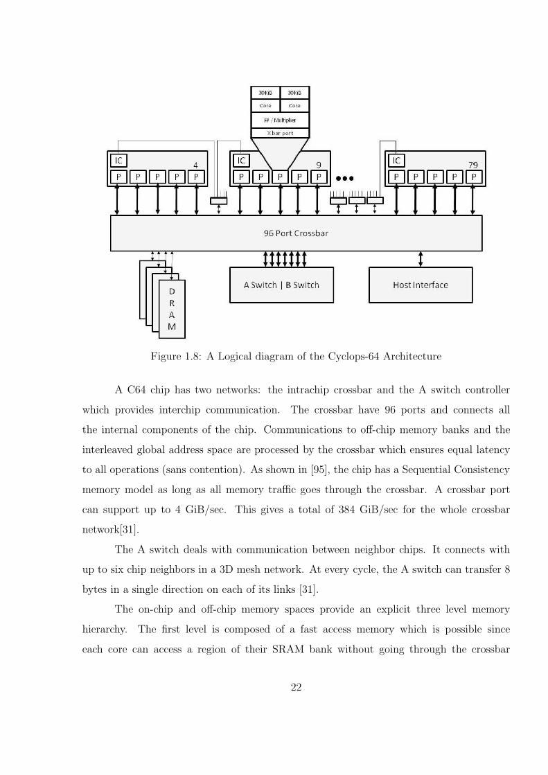
Figure 1.8: A Logical diagram of the Cyclops-64 Architecture
A C64 chip has two networks: the intrachip crossbar and the A switch controller
which provides interchip communication. The crossbar have 96 ports and connects all
the internal components of the chip. Communications to off-chip memory banks and the
interleaved global address space are processed by the crossbar which ensures equal latency
to all operations (sans contention). As shown in [95], the chip has a Sequential Consistency
memory model as long as all memory traffic goes through the crossbar. A crossbar port
can support up to 4 GiB/sec. This gives a total of 384 GiB/sec for the whole crossbar
network[31].
The A switch deals with communication between neighbor chips. It connects with
up to six chip neighbors in a 3D mesh network. At every cycle, the A switch can transfer 8
bytes in a single direction on each of its links [31].
The on-chip and off-chip memory spaces provide an explicit three level memory
hierarchy. The first level is composed of a fast access memory which is possible since
each core can access a region of their SRAM bank without going through the crossbar
22
controller. This space is called the Scratch pad memory and it can be configured at boot
time. Moreover, this space is considered private to its connected cores16. The rest of
the SRAM bank is part of the interleaved global SRAM which is accessible by all cores.
Finally, we have the DRAM memory space which is the off-chip memory which has the
longest latency. Access to global SRAM and DRAM are Sequentially Consistent. However,
accesses to Scratch pad are not[95].
The chip does not have any hardware data cache, does not support virtual memory or
DMA engines for intra-chip communication. All memory accesses must be orchestrated by
the programmer (or runtime system). Application development for the Cyclops64 is helped
by an easy-to-use tool-chain, a micro-kernel and a high performance runtime system. Some
other important features of the architecture includes: hardware support for barriers, a light
weight threading model, called Tiny Threads, and several atomic primitives used to perform
operations in memory. The final system (composed of 24 by 24 by 24 nodes) will be capable
of over one petaFLOP of computing power [31].
All these designs show the way that processor and interconnect technologies work
together to ensure the habitation of dozen of processing elements. However, we must in-
troduce the other camp of parallel computing design: heterogeneous designs. Under these
designs, several different architectural types come together on a single die. The major fea-
ture of these designs, their heterogeneity, it is also their major weakness. Coordinating
all the elements of the design is a very difficult task to do either automatically or by the
programmer. This reduces the productivity of a system greatly and the need for software
infrastructure is essential for the survival of the design. In Chapter 3.3, the architecture
used in this study and its software infrastructure are introduced. However, before we jump
to this, we need to introduce the questions that this thesis tries to answer; and we introduce
the elusive concept of productivity to the readers (Chapter 2).
16 However it can be access by other cores if needed
23
1.2 Problem Formulation: an Overview
Thanks to current trends, many of the old problems of yesteryears have come back
to haunt system designers and programmers. One of these problems is how to utilize effi-
ciently utilize the limited memory which each of the accelerator / co-processor units have?
Moreover, when a design is proposed, how to effectively optimize such a design so that it
can provide the maximum performance available?
Many frameworks have been designed to answer these questions. Several of them
are mentioned when in Chapter 7. This thesis answers the first question by proposing a
framework that loads code on demand. This solution is not novel since the concept of
overlays and partitions were used before the advent of virtual memory. However, their im-
plementation to the heterogeneous architectures is a novel idea. Moreover, the overlays and
partitions introduced here have a much finer granularity and a wider range of uses than the
ones provided by classical overlays, embedded systems overlays or even by virtual memory.
The second question is answered by several replacements methods that aim to minimize
long latency operations. The next sections and chapters introduce both the problems and
the proposed solutions further.
1.3 Contributions
This thesis’s framework was designed to increase programmability in the Cell B.E.
architecture. In its current iteration, many optimization efforts are under way for each com-
ponent. Two of the most performance-heavy components and the target of many of these
optimization efforts are the partition manager and the software cache. Both of these com-
ponents use Direct Memory Accesses (a.k.a. DMAs) transfers heavily. Thus, the objective
of all these efforts is to minimize the number of DMA transactions per given application.
This thesis main objective is to present a framework which provides support for dynamic
migrating code for many core architectures using the partition manager framework. To this
purpose some code overlaying techniques are presented. These techniques range from divi-
sion of the available overlay space through different replacement polices. The contributions
of this thesis are as follows.
24
1. The development of a framework that loads and manages partitions across function
calls. In this manner, the restricted memory problem can be alleviated and the range
of applications that can be run on the co-processing unit is expanded.
2. The implementation of replacement policies that are useful to reduce the number of
DMA transfers across partitions. Such replacement policies aim to optimize the most
costly operations in the proposed framework. Such replacements can be of the form
of buffer divisions, rules about eviction and loading, etc.
3. A quantification of such replacement policies given a selected set of applications and a
report of the overhead of such policies. Several policies can be given but a quantitative
study is necessary to analyze which policy is best for which application since the code
can have different behaviors.
4. An API which can be easily ported and extended to several types of architectures.
The problem of restricted space is not going away. The new trend seems to favor an
increasing number of cores (with local memories) instead of more hardware features
and heavy system software. This means that frameworks like the one proposed in
this thesis will become more and more important as the wave of multi / many core
continues its ascent.
5. A productivity study which tries to define the elusive concept of productivity with a
set of metrics and the introduction of expertise as weighting functions.
This thesis is organized as follows. The next chapter (2) introduces the concept
of productivity and their place in High Performance Computing. Chapter 3 has a short
overview on the Cell Broadband engine architecture and the Open Opell framework. Chap-
ter 4 presents the changes to the toolchain and a very brief overview of the partition manager
framework. Chapter 5 shows the lazy reused (cache like) replacement policies and shows the
25

replacement policies with pre-fetching methods and introduces the partition graph struc-
ture. Chapter 6 presents the experimental framework and testbed. Chapter 7 shows related
work to this thesis. Chapter 8 presents the conclusions drawn from this work.
26
Chapter 2
PRODUCTIVITY STUDIES
“While computer performance has improved dramatically, real productivityin terms of the science accomplished with these ever-faster machines has notkept pace. Indeed, scientists are finding it increasingly costly and time con-suming to write, port, or rewrite their software to take advantage of the newhardware. While machine performance remains a critical productivity driver forhigh-performance computing applications, software development time increas-ingly dominates hardware speed as the primary productivity bottleneck” [37]
As new generations of multi / many core designs rise and fall, an old problem raises
its head: productivity. In layman terms, productivity refers to the production of a unit
of work in a specified amount of time. Under the High Performance Computing (HPC)
field, this objective is harder to achieve due to the challenges imposed by the new design
decisions which move many classical hardware features (i.e. coherent caches, hardware
virtual memory, automatic data layout and movement, etc) to the software stack. As a
result of these challenges, the High Productivity Computing System (HPCS) project led
by DARPA was created. This is not much different than current projects which deal with
hardware / software co-design issues like the Ubiquitous High Performance Computing
(UHPC) initiative, also lead by DARPA[29].
With all these considerations in mind, emergent parallel programming models need
to be carefully crafted to take advantage of the underlying hardware architecture and be
intuitive enough to be accepted by seasoned and novice programmers alike. One of the se-
lected groups for the HPCS project is the IBM’s Productive Easy-to-Use Reliable Computer
Systems (PERCS) initiative. This group created several methods to empirically measure
the productivity of selected parallel languages or languages’ features. These methods be-
came fundamental on their overview of language design. A graphical representation of such
27
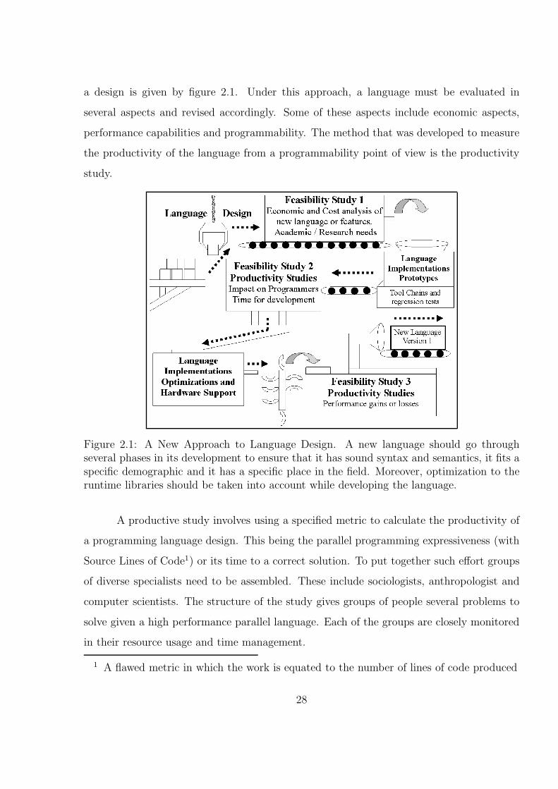
a design is given by figure 2.1. Under this approach, a language must be evaluated in
several aspects and revised accordingly. Some of these aspects include economic aspects,
performance capabilities and programmability. The method that was developed to measure
the productivity of the language from a programmability point of view is the productivity
study.
Figure 2.1: A New Approach to Language Design. A new language should go throughseveral phases in its development to ensure that it has sound syntax and semantics, it fits aspecific demographic and it has a specific place in the field. Moreover, optimization to theruntime libraries should be taken into account while developing the language.
A productive study involves using a specified metric to calculate the productivity of
a programming language design. This being the parallel programming expressiveness (with
Source Lines of Code1) or its time to a correct solution. To put together such effort groups
of diverse specialists need to be assembled. These include sociologists, anthropologist and
computer scientists. The structure of the study gives groups of people several problems to
solve given a high performance parallel language. Each of the groups are closely monitored
in their resource usage and time management.
1 A flawed metric in which the work is equated to the number of lines of code produced
28
One of the most difficult aspects of parallel programming is synchronization. These
features are designed to restrict the famous data race problem in which two or more concur-
rent memory operations (and at least one of them is a write) can affect each other resulting
value. This creates non determinism that is not acceptable by most applications and al-
gorithms2. In modern programming models, the synchronization primitives take the form
of lock / unlock operations and critical sections. An effect of these constructs in produc-
tivity is that they put excessive resource management requirements on the programmer.
Thus, the probability that logical errors appear increases. Moreover, according to which
programming model is used, these constructs will have hidden costs to keep consistency
and coherence of their protected data and internal structures[75]. Such overhead limits
the scalable parallelism that could be achieved. For these reasons, Atomic Sections (A.S.)
were proposed to provide a more intuitive way to synchronize regions of code with minimal
performance overhead [94]. The construct was implemented in the C language and it be-
haves like an acquire / release region under entry consistency[73] as far as their consistency
actions are concerned. Moreover, it provides the mutual exclusion and atomicity required
by the region. This construct was implemented in the OpenMP XN framework using the
Omni source-to-source compiler. More detailed explanation about A.S. can be found on
subsection 2.1. Using this new construct, we developed a productivity study (The Delaware
Programmability, Productivity and Proficiency Inquiry or P3I) to measure empirically its
effect on time to correct solution. One of this study salient feature is the introduction of
weights to the framework which will prune to the data according to the study’s point of
interest. This section shows the productivity study framework and initial results. However,
an short overview of Atomic Sections is required.
2 There are some algorithms that allows certain amount of error in their computation forwhich the cost of synchronization might be too expensive and / or the probability ofthe data race occurring is very low[11]
29
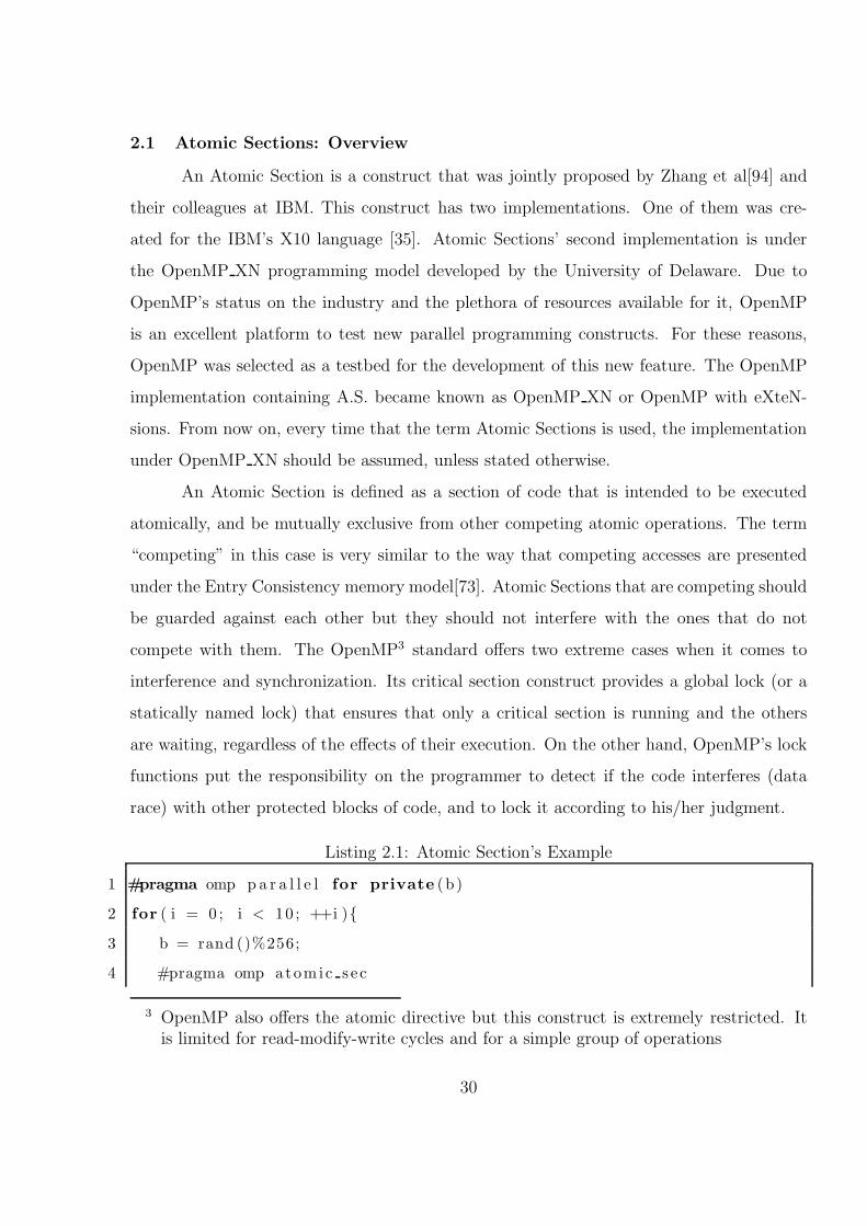
2.1 Atomic Sections: Overview
An Atomic Section is a construct that was jointly proposed by Zhang et al[94] and
their colleagues at IBM. This construct has two implementations. One of them was cre-
ated for the IBM’s X10 language [35]. Atomic Sections’ second implementation is under
the OpenMP XN programming model developed by the University of Delaware. Due to
OpenMP’s status on the industry and the plethora of resources available for it, OpenMP
is an excellent platform to test new parallel programming constructs. For these reasons,
OpenMP was selected as a testbed for the development of this new feature. The OpenMP
implementation containing A.S. became known as OpenMP XN or OpenMP with eXteN-
sions. From now on, every time that the term Atomic Sections is used, the implementation
under OpenMP XN should be assumed, unless stated otherwise.
An Atomic Section is defined as a section of code that is intended to be executed
atomically, and be mutually exclusive from other competing atomic operations. The term
“competing” in this case is very similar to the way that competing accesses are presented
under the Entry Consistency memory model[73]. Atomic Sections that are competing should
be guarded against each other but they should not interfere with the ones that do not
compete with them. The OpenMP3 standard offers two extreme cases when it comes to
interference and synchronization. Its critical section construct provides a global lock (or a
statically named lock) that ensures that only a critical section is running and the others
are waiting, regardless of the effects of their execution. On the other hand, OpenMP’s lock
functions put the responsibility on the programmer to detect if the code interferes (data
race) with other protected blocks of code, and to lock it according to his/her judgment.
Listing 2.1: Atomic Section’s Example
1 #pragma omp p a r a l l e l for private (b)
2 for ( i = 0 ; i < 10 ; ++i ){
3 b = rand ()%256;
4 #pragma omp atomic s ec
3 OpenMP also offers the atomic directive but this construct is extremely restricted. Itis limited for read-modify-write cycles and for a simple group of operations
30
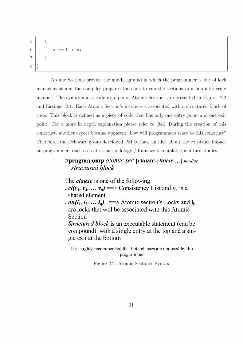
5 {
6 a += b ∗ c ;
7 }
8 }
Atomic Sections provide the middle ground in which the programmer is free of lock
management and the compiler prepares the code to run the sections in a non-interfering
manner. The syntax and a code example of Atomic Sections are presented in Figure 2.2
and Listings 2.1. Each Atomic Section’s instance is associated with a structured block of
code. This block is defined as a piece of code that has only one entry point and one exit
point. For a more in depth explanation please refer to [94]. During the creation of this
construct, another aspect became apparent: how will programmers react to this construct?
Therefore, the Delaware group developed P3I to have an idea about the construct impact
on programmers and to create a methodology / framework template for future studies.
Figure 2.2: Atomic Section’s Syntax
31
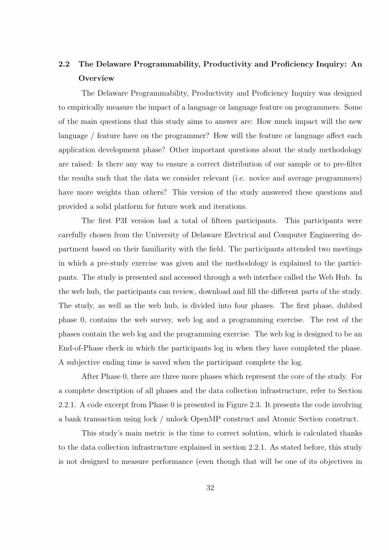
2.2 The Delaware Programmability, Productivity and Proficiency Inquiry: An
Overview
The Delaware Programmability, Productivity and Proficiency Inquiry was designed
to empirically measure the impact of a language or language feature on programmers. Some
of the main questions that this study aims to answer are: How much impact will the new
language / feature have on the programmer? How will the feature or language affect each
application development phase? Other important questions about the study methodology
are raised: Is there any way to ensure a correct distribution of our sample or to pre-filter
the results such that the data we consider relevant (i.e. novice and average programmers)
have more weights than others? This version of the study answered these questions and
provided a solid platform for future work and iterations.
The first P3I version had a total of fifteen participants. This participants were
carefully chosen from the University of Delaware Electrical and Computer Engineering de-
partment based on their familiarity with the field. The participants attended two meetings
in which a pre-study exercise was given and the methodology is explained to the partici-
pants. The study is presented and accessed through a web interface called the Web Hub. In
the web hub, the participants can review, download and fill the different parts of the study.
The study, as well as the web hub, is divided into four phases. The first phase, dubbed
phase 0, contains the web survey, web log and a programming exercise. The rest of the
phases contain the web log and the programming exercise. The web log is designed to be an
End-of-Phase check in which the participants log in when they have completed the phase.
A subjective ending time is saved when the participant complete the log.
After Phase 0, there are three more phases which represent the core of the study. For
a complete description of all phases and the data collection infrastructure, refer to Section
2.2.1. A code excerpt from Phase 0 is presented in Figure 2.3. It presents the code involving
a bank transaction using lock / unlock OpenMP construct and Atomic Section construct.
This study’s main metric is the time to correct solution, which is calculated thanks
to the data collection infrastructure explained in section 2.2.1. As stated before, this study
is not designed to measure performance (even though that will be one of its objectives in
32
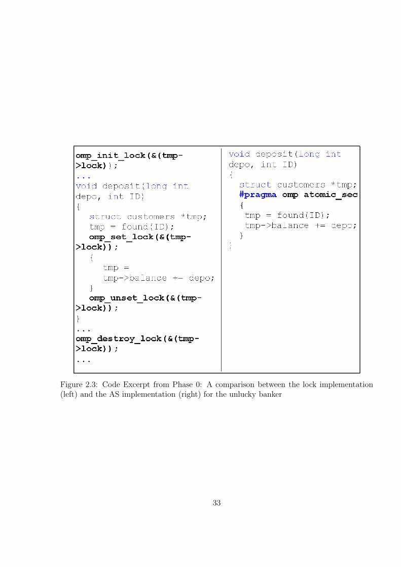
Figure 2.3: Code Excerpt from Phase 0: A comparison between the lock implementation(left) and the AS implementation (right) for the unlucky banker
33
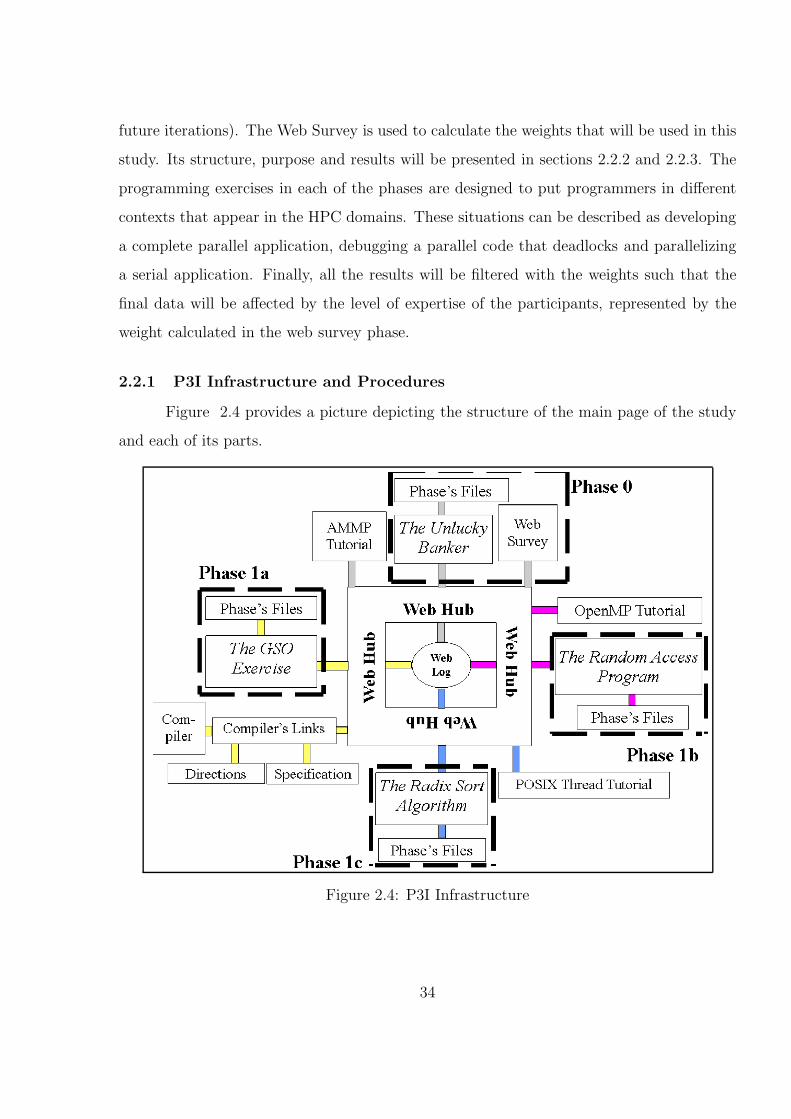
future iterations). The Web Survey is used to calculate the weights that will be used in this
study. Its structure, purpose and results will be presented in sections 2.2.2 and 2.2.3. The
programming exercises in each of the phases are designed to put programmers in different
contexts that appear in the HPC domains. These situations can be described as developing
a complete parallel application, debugging a parallel code that deadlocks and parallelizing
a serial application. Finally, all the results will be filtered with the weights such that the
final data will be affected by the level of expertise of the participants, represented by the
weight calculated in the web survey phase.
2.2.1 P3I Infrastructure and Procedures
Figure 2.4 provides a picture depicting the structure of the main page of the study
and each of its parts.
Figure 2.4: P3I Infrastructure
34
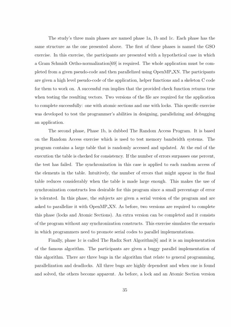
The study’s three main phases are named phase 1a, 1b and 1c. Each phase has the
same structure as the one presented above. The first of these phases is named the GSO
exercise. In this exercise, the participants are presented with a hypothetical case in which
a Gram Schmidt Ortho-normalization[69] is required. The whole application must be com-
pleted from a given pseudo-code and then parallelized using OpenMP XN. The participants
are given a high level pseudo-code of the application, helper functions and a skeleton C code
for them to work on. A successful run implies that the provided check function returns true
when testing the resulting vectors. Two versions of the file are required for the application
to complete successfully: one with atomic sections and one with locks. This specific exercise
was developed to test the programmer’s abilities in designing, parallelizing and debugging
an application.
The second phase, Phase 1b, is dubbed The Random Access Program. It is based
on the Random Access exercise which is used to test memory bandwidth systems. The
program contains a large table that is randomly accessed and updated. At the end of the
execution the table is checked for consistency. If the number of errors surpasses one percent,
the test has failed. The synchronization in this case is applied to each random access of
the elements in the table. Intuitively, the number of errors that might appear in the final
table reduces considerably when the table is made large enough. This makes the use of
synchronization constructs less desirable for this program since a small percentage of error
is tolerated. In this phase, the subjects are given a serial version of the program and are
asked to parallelize it with OpenMP XN. As before, two versions are required to complete
this phase (locks and Atomic Sections). An extra version can be completed and it consists
of the program without any synchronization constructs. This exercise simulates the scenario
in which programmers need to promote serial codes to parallel implementations.
Finally, phase 1c is called The Radix Sort Algorithm[6] and it is an implementation
of the famous algorithm. The participants are given a buggy parallel implementation of
this algorithm. There are three bugs in the algorithm that relate to general programming,
parallelization and deadlocks. All three bugs are highly dependent and when one is found
and solved, the others become apparent. As before, a lock and an Atomic Section version
35
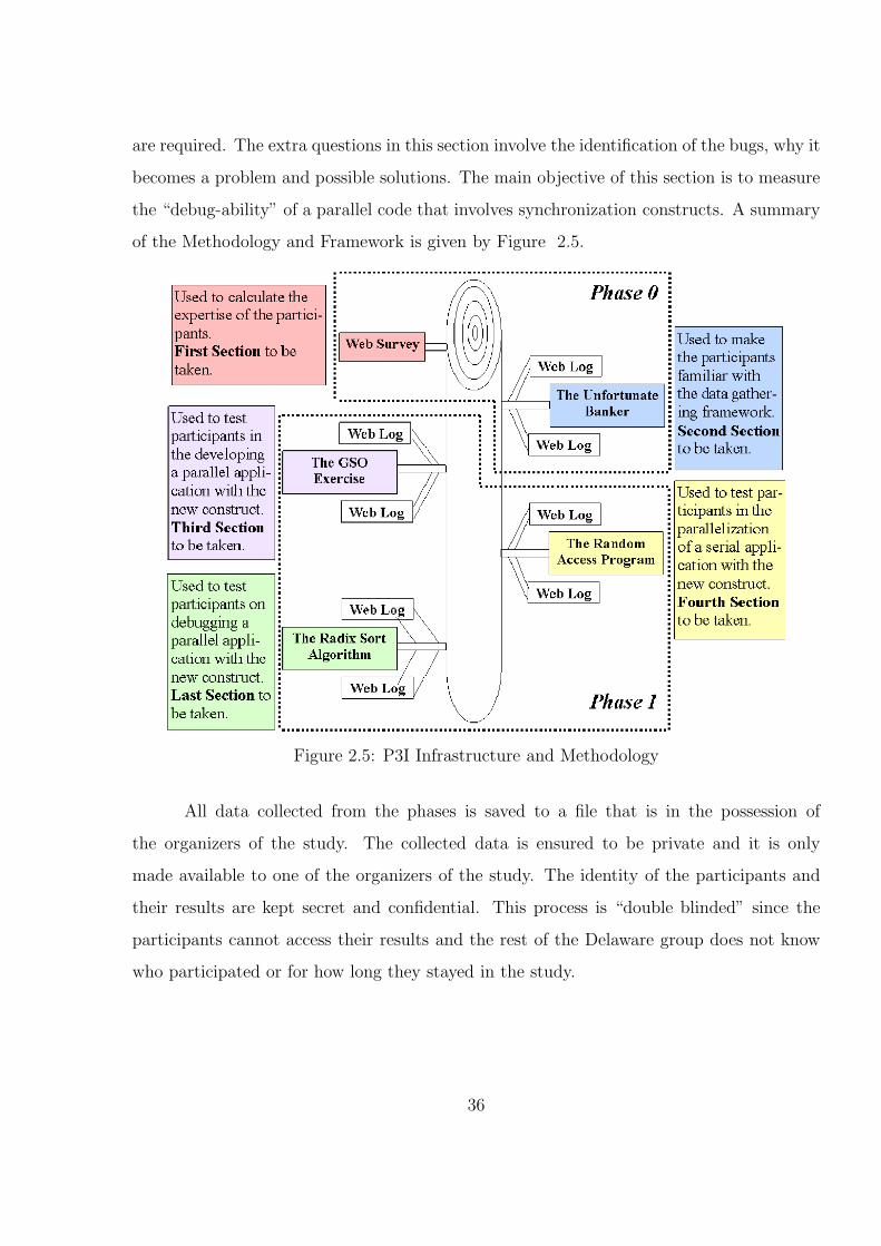
are required. The extra questions in this section involve the identification of the bugs, why it
becomes a problem and possible solutions. The main objective of this section is to measure
the “debug-ability” of a parallel code that involves synchronization constructs. A summary
of the Methodology and Framework is given by Figure 2.5.
Figure 2.5: P3I Infrastructure and Methodology
All data collected from the phases is saved to a file that is in the possession of
the organizers of the study. The collected data is ensured to be private and it is only
made available to one of the organizers of the study. The identity of the participants and
their results are kept secret and confidential. This process is “double blinded” since the
participants cannot access their results and the rest of the Delaware group does not know
who participated or for how long they stayed in the study.
36
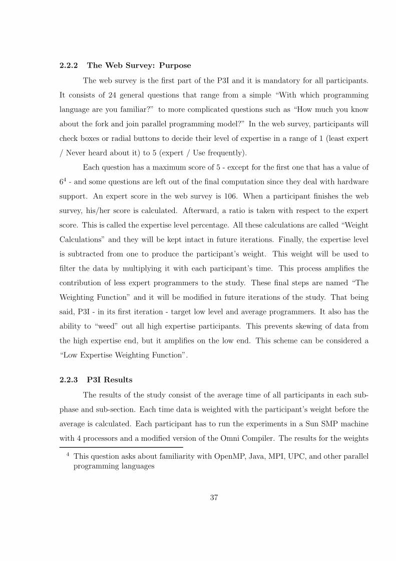
2.2.2 The Web Survey: Purpose
The web survey is the first part of the P3I and it is mandatory for all participants.
It consists of 24 general questions that range from a simple “With which programming
language are you familiar?” to more complicated questions such as “How much you know
about the fork and join parallel programming model?” In the web survey, participants will
check boxes or radial buttons to decide their level of expertise in a range of 1 (least expert
/ Never heard about it) to 5 (expert / Use frequently).
Each question has a maximum score of 5 - except for the first one that has a value of
64 - and some questions are left out of the final computation since they deal with hardware
support. An expert score in the web survey is 106. When a participant finishes the web
survey, his/her score is calculated. Afterward, a ratio is taken with respect to the expert
score. This is called the expertise level percentage. All these calculations are called “Weight
Calculations” and they will be kept intact in future iterations. Finally, the expertise level
is subtracted from one to produce the participant’s weight. This weight will be used to
filter the data by multiplying it with each participant’s time. This process amplifies the
contribution of less expert programmers to the study. These final steps are named “The
Weighting Function” and it will be modified in future iterations of the study. That being
said, P3I - in its first iteration - target low level and average programmers. It also has the
ability to “weed” out all high expertise participants. This prevents skewing of data from
the high expertise end, but it amplifies on the low end. This scheme can be considered a
“Low Expertise Weighting Function”.
2.2.3 P3I Results
The results of the study consist of the average time of all participants in each sub-
phase and sub-section. Each time data is weighted with the participant’s weight before the
average is calculated. Each participant has to run the experiments in a Sun SMP machine
with 4 processors and a modified version of the Omni Compiler. The results for the weights
4 This question asks about familiarity with OpenMP, Java, MPI, UPC, and other parallelprogramming languages
37
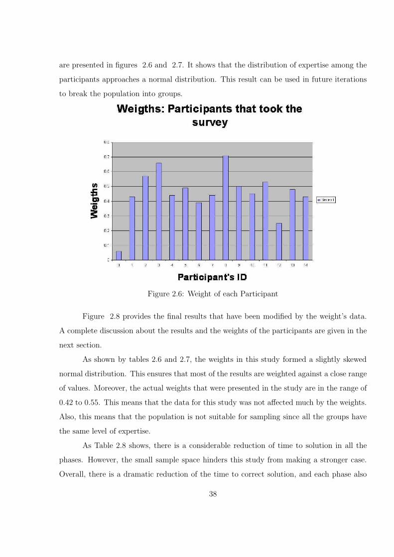
are presented in figures 2.6 and 2.7. It shows that the distribution of expertise among the
participants approaches a normal distribution. This result can be used in future iterations
to break the population into groups.
Figure 2.6: Weight of each Participant
Figure 2.8 provides the final results that have been modified by the weight’s data.
A complete discussion about the results and the weights of the participants are given in the
next section.
As shown by tables 2.6 and 2.7, the weights in this study formed a slightly skewed
normal distribution. This ensures that most of the results are weighted against a close range
of values. Moreover, the actual weights that were presented in the study are in the range of
0.42 to 0.55. This means that the data for this study was not affected much by the weights.
Also, this means that the population is not suitable for sampling since all the groups have
the same level of expertise.
As Table 2.8 shows, there is a considerable reduction of time to solution in all the
phases. However, the small sample space hinders this study from making a stronger case.
Overall, there is a dramatic reduction of the time to correct solution, and each phase also
38
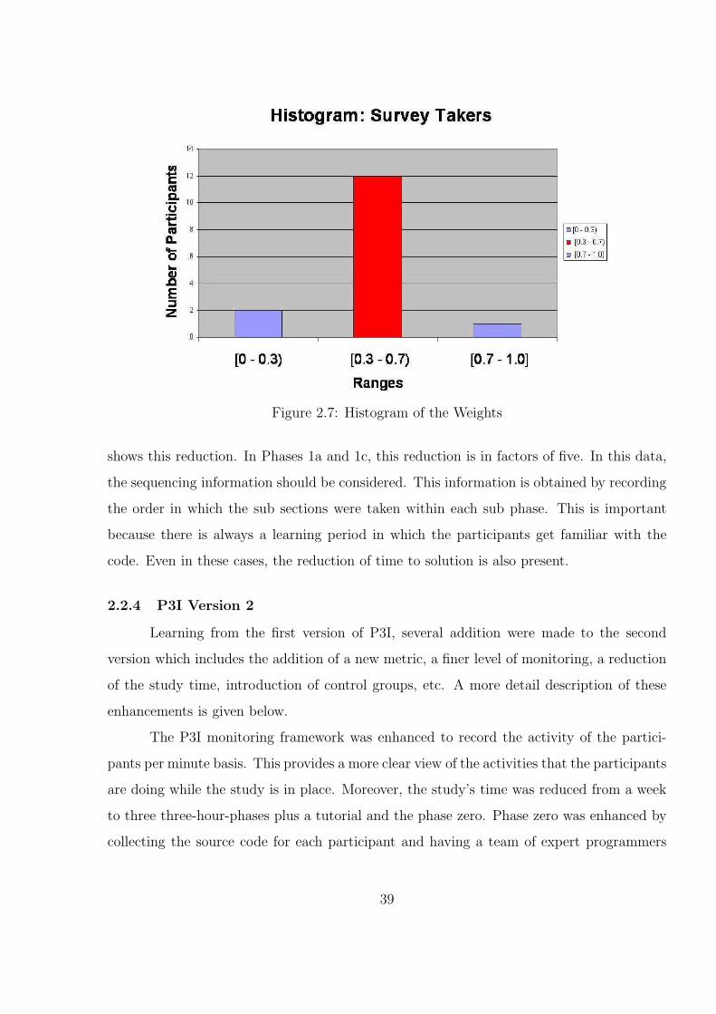
Figure 2.7: Histogram of the Weights
shows this reduction. In Phases 1a and 1c, this reduction is in factors of five. In this data,
the sequencing information should be considered. This information is obtained by recording
the order in which the sub sections were taken within each sub phase. This is important
because there is always a learning period in which the participants get familiar with the
code. Even in these cases, the reduction of time to solution is also present.
2.2.4 P3I Version 2
Learning from the first version of P3I, several addition were made to the second
version which includes the addition of a new metric, a finer level of monitoring, a reduction
of the study time, introduction of control groups, etc. A more detail description of these
enhancements is given below.
The P3I monitoring framework was enhanced to record the activity of the partici-
pants per minute basis. This provides a more clear view of the activities that the participants
are doing while the study is in place. Moreover, the study’s time was reduced from a week
to three three-hour-phases plus a tutorial and the phase zero. Phase zero was enhanced by
collecting the source code for each participant and having a team of expert programmers
39
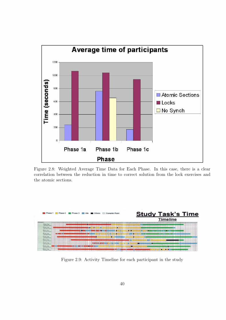
Figure 2.8: Weighted Average Time Data for Each Phase. In this case, there is a clearcorrelation between the reduction in time to correct solution from the lock exercises andthe atomic sections.
Figure 2.9: Activity Timeline for each participant in the study
40
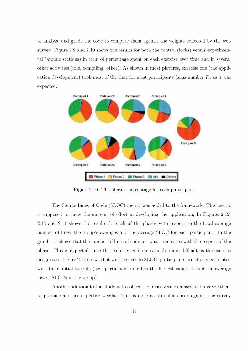
to analyze and grade the code to compare them against the weights collected by the web
survey. Figure 2.9 and 2.10 shows the results for both the control (locks) versus experimen-
tal (atomic sections) in term of percentage spent on each exercise over time and in several
other activities (idle, compiling, other). As shown in most pictures, exercise one (the appli-
cation development) took most of the time for most participants (sans number 7), as it was
expected.
Figure 2.10: The phase’s percentage for each participant
The Source Lines of Code (SLOC) metric was added to the framework. This metric
is supposed to show the amount of effort in developing the application, In Figures 2.12,
2.13 and 2.11 shows the results for each of the phases with respect to the total average
number of lines, the group’s averages and the average SLOC for each participant. In the
graphs, it shows that the number of lines of code per phase increases with the respect of the
phase. This is expected since the exercises gets increasingly more difficult as the exercise
progresses. Figure 2.11 shows that with respect to SLOC, participants are closely correlated
with their initial weights (e.g. participant nine has the highest expertise and the average
lowest SLOCs in the group).
Another addition to the study is to collect the phase zero exercises and analyze them
to produce another expertise weight. This is done as a double check against the survey
41
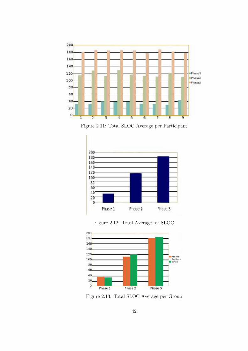
Figure 2.11: Total SLOC Average per Participant
Figure 2.12: Total Average for SLOC
Figure 2.13: Total SLOC Average per Group
42
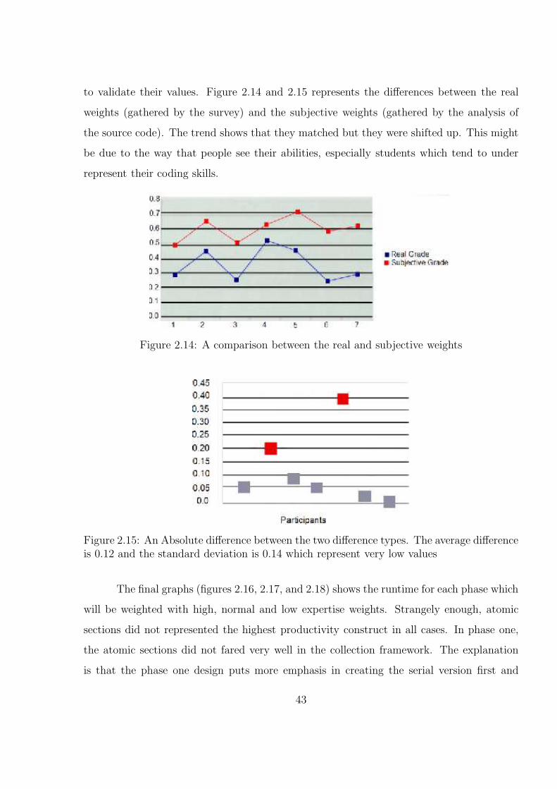
to validate their values. Figure 2.14 and 2.15 represents the differences between the real
weights (gathered by the survey) and the subjective weights (gathered by the analysis of
the source code). The trend shows that they matched but they were shifted up. This might
be due to the way that people see their abilities, especially students which tend to under
represent their coding skills.
Figure 2.14: A comparison between the real and subjective weights
Figure 2.15: An Absolute difference between the two difference types. The average differenceis 0.12 and the standard deviation is 0.14 which represent very low values
The final graphs (figures 2.16, 2.17, and 2.18) shows the runtime for each phase which
will be weighted with high, normal and low expertise weights. Strangely enough, atomic
sections did not represented the highest productivity construct in all cases. In phase one,
the atomic sections did not fared very well in the collection framework. The explanation
is that the phase one design puts more emphasis in creating the serial version first and
43
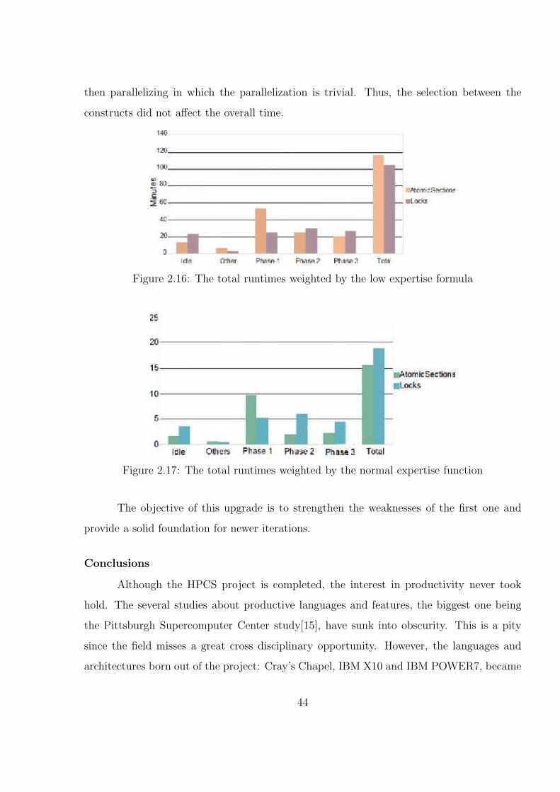
then parallelizing in which the parallelization is trivial. Thus, the selection between the
constructs did not affect the overall time.
Figure 2.16: The total runtimes weighted by the low expertise formula
Figure 2.17: The total runtimes weighted by the normal expertise function
The objective of this upgrade is to strengthen the weaknesses of the first one and
provide a solid foundation for newer iterations.
Conclusions
Although the HPCS project is completed, the interest in productivity never took
hold. The several studies about productive languages and features, the biggest one being
the Pittsburgh Supercomputer Center study[15], have sunk into obscurity. This is a pity
since the field misses a great cross disciplinary opportunity. However, the languages and
architectures born out of the project: Cray’s Chapel, IBM X10 and IBM POWER7, became
44
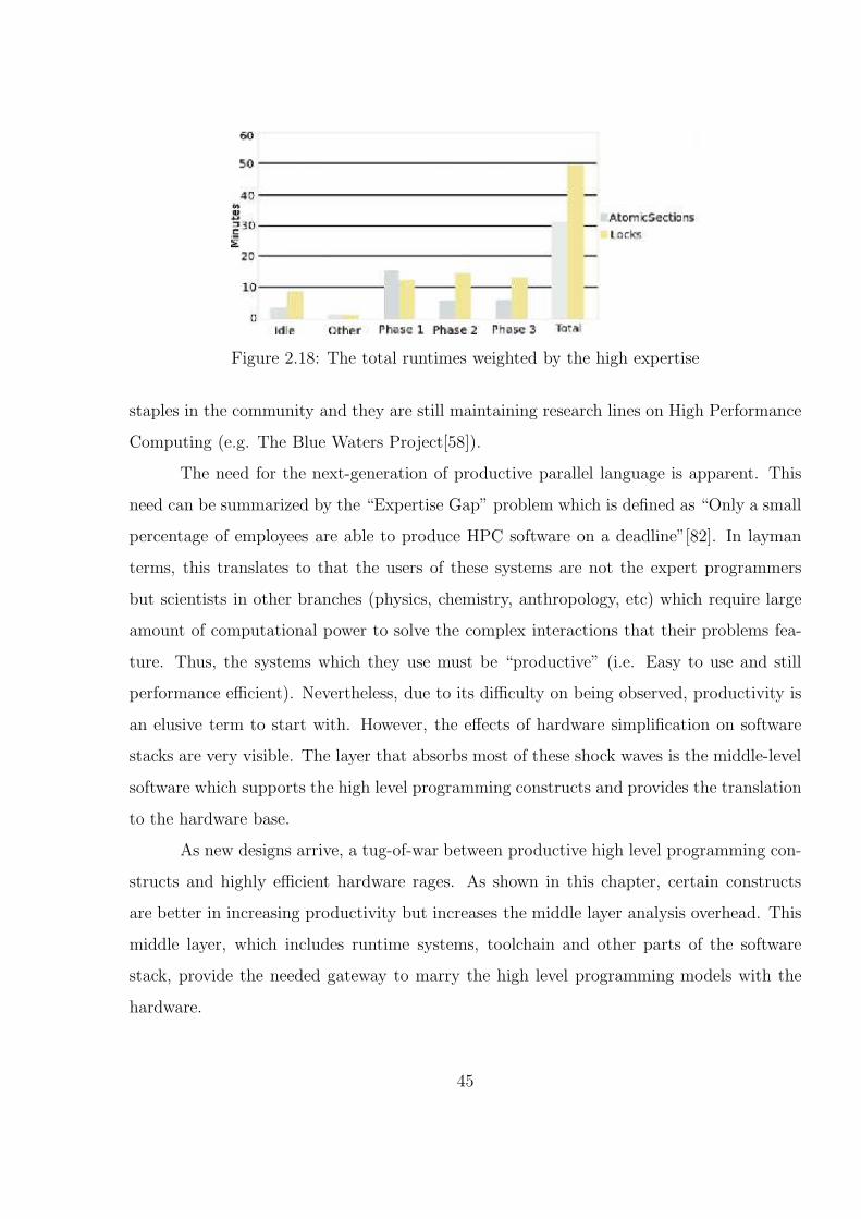
Figure 2.18: The total runtimes weighted by the high expertise
staples in the community and they are still maintaining research lines on High Performance
Computing (e.g. The Blue Waters Project[58]).
The need for the next-generation of productive parallel language is apparent. This
need can be summarized by the “Expertise Gap” problem which is defined as “Only a small
percentage of employees are able to produce HPC software on a deadline”[82]. In layman
terms, this translates to that the users of these systems are not the expert programmers
but scientists in other branches (physics, chemistry, anthropology, etc) which require large
amount of computational power to solve the complex interactions that their problems fea-
ture. Thus, the systems which they use must be “productive” (i.e. Easy to use and still
performance efficient). Nevertheless, due to its difficulty on being observed, productivity is
an elusive term to start with. However, the effects of hardware simplification on software
stacks are very visible. The layer that absorbs most of these shock waves is the middle-level
software which supports the high level programming constructs and provides the translation
to the hardware base.
As new designs arrive, a tug-of-war between productive high level programming con-
structs and highly efficient hardware rages. As shown in this chapter, certain constructs
are better in increasing productivity but increases the middle layer analysis overhead. This
middle layer, which includes runtime systems, toolchain and other parts of the software
stack, provide the needed gateway to marry the high level programming models with the
hardware.
45
For this purpose, we selected a notoriously difficult to use architecture, but proven
to be highly efficient: the Cell Broadband Engine and we ported one of the most used and
productive Programming models, OpenMP (as shown in this chapter) to it. This effort is
called the Open Opell project at the University of Delaware [60][67][68]. In this way, we can
married a highly productive language, i.e. OpenMP, and a novel runtime system designed
to replace and optimize missing hardware features.
46
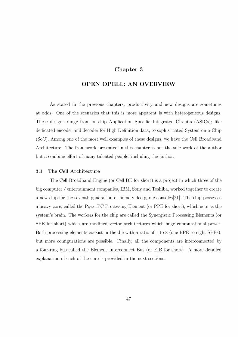
Chapter 3
OPEN OPELL: AN OVERVIEW
As stated in the previous chapters, productivity and new designs are sometimes
at odds. One of the scenarios that this is more apparent is with heterogeneous designs.
These designs range from on-chip Application Specific Integrated Circuits (ASICs); like
dedicated encoder and decoder for High Definition data, to sophisticated System-on-a-Chip
(SoC). Among one of the most well examples of these designs, we have the Cell Broadband
Architecture. The framework presented in this chapter is not the sole work of the author
but a combine effort of many talented people, including the author.
3.1 The Cell Architecture
The Cell Broadband Engine (or Cell BE for short) is a project in which three of the
big computer / entertainment companies, IBM, Sony and Toshiba, worked together to create
a new chip for the seventh generation of home video game consoles[21]. The chip possesses
a heavy core, called the PowerPC Processing Element (or PPE for short), which acts as the
system’s brain. The workers for the chip are called the Synergistic Processing Elements (or
SPE for short) which are modified vector architectures which huge computational power.
Both processing elements coexist in the die with a ratio of 1 to 8 (one PPE to eight SPEs),
but more configurations are possible. Finally, all the components are interconnected by
a four-ring bus called the Element Interconnect Bus (or EIB for short). A more detailed
explanation of each of the core is provided in the next sections.
47
Figure 3.1: Block Diagram of the Cell Broadband engine. This figure shows the blockdiagram of the Cell B.E. and its components (PPE and SPE). It also shows the internalstructures for the SPE pipelines and a high overview graph of the interconnect bus.
48
3.1.1 The PowerPC Processing Element
Commonly referred as the PPE, this element is an example of a heavy core. It is
a POWERPC chip complete with Virtual memory support, coherent caches, vector exten-
sions, two-way multithreaded, among other hardware features. The complete definition for
the PPE can found on the POWERPC Architecture Books I to III [70]. Besides being a
POWERPC core, it has certain optional features (Altivec unit, floating point reciprocate
estimate and square root, and an added cache line operation) to help it with multimedia
application processing. Some other features include a data and instruction level 1 (32 /32
KiB) cache, a unified level 2 cache (512 KiB, 8-way set associative) and a 2-bit branch
prediction hardware.
Although the PPE is an in-order machine, they have several “tricks” that allows to
reap the benefits of an out of order execution engine. Some of these are delayed execution
pipelines and the ability to issue up to eight outstanding loads[70]. On most of the current
configurations, it runs at 3.2 GHz. As the brain of the system, it runs the Operating System
and has access to all the memory spaces 1. Its purpose can be summarized as an orchestrator
of resources (these include the SPEs, their memories, the EIB and main memory, as well as
any I/O devices).
The final component of the PPE is the PowerPC Processor Storage Subsystem
(PPSS). This component handles every memory request that need to be coherent between
the PPE and the Element Interconnect Bus (EIB). An interesting note is that, although the
computational engine internal memory (referred as local storage below) does not need to be
coherent, most of the requests (which are DMA operations) to and from main memory must
be made so. The PPSS hosts the PPE’s unified level 2 cache. Moreover, it controls pacing
for the EIB and does pre-fetching for the PPU. Finally, it has access to the Resource Allo-
cator Management and the Replacement Management Tables (used by both the Cache and
the TLB). Control over both structures is handy when doing real time programming[21].
The block diagram of the PPE is shown in the lower parts of Figure 3.1.
1 Real (all physical memory), Virtual (virtual addressing space) and Effective (all of theabove plus any memory mapped I/O)
49
3.1.2 The Synergistic Processing Element
Commonly referred as the SPE, this element is a simple core, plus an enhanced
memory management unit, which serves as a computational engine for the Cell. A SPE is
divided into the Synergistic Processing Unit (SPU) and its Memory Flow Controller (MFC).
The unit is a modified vector architecture which can run general purpose code (with a certain
performance penalty) but it shines when dealing with vector applications. It is an in-order,
(very limited) dual issue chip. It has a 128 times 128 bits register file, 256 KiB of local
storage, and a dual pipeline (named even and odd). An SPU can only work on data and
code which reside in its local storage (using load and store operations). Although it lacks
the advance branch prediction mechanism of the PPU, it allows branch hints to be inserted
in the code to better utilize the pipelines.
To access main memory and other local storage locations, a special channel interface
and the Memory Flow Controller are used. A side note is that the local storage of each
SPU is a non cacheable region. This means that even if it is mapped to main memory, it
will not be kept consistent / coherent across SPUs and other components of the system[21].
However, as stated before, every MFC requests will be coherent. To access main memory,
the SPU depends on a group of Direct Memory Address (DMA) operations. As classically
stated, the DMA is an asynchronous memory transfer from a remote location to a near
one[21]. In this case, the remote location is the off chip main memory or another SPE’s
local storage. In the SPU, the DMA operations can be grouped using numerical tags (with a
maximum of 32 tags available to the programmer). These tags are used to ensure completion
time or an order between the DMA transfers (using barrier and fence semantics[21]).
The DMA transfers, as well as other channel operations, i.e. signal and mailboxes;
are taken care by the Memory Flow Controller (MFC) part of the SPU. The main purpose
of this component is to ensure that data (or code) is delivered safely from and to the Local
Storage of the given SPU. It possesses its own set of registers, two command queues (one for
local SPU commands and one for outside ones), a Memory Management Unit, a Memory
Mapped I/O (MMIO) interface, and a copy of the Replacement Management Table (RMT).
Unlike the SPU, the MFC must be aware of the state of all memory spaces (virtual, effective
50
and real). Thus, it must have knowledge of the virtual tables and any MMIO mapping
(including, but not limited, to the mapping of LS onto main memory space). Finally, the
MFC has a TLB and a cache for atomic operations which can be managed by PPE privileged
software[21].
A single SPU (first generation) is capable of 25.6 Gflops of peak performance in
Single Precision Mode. However, for first generation chips, the double point performance
drops considerable from 25.6 to 1.8 GFLOPS [21].
3.1.3 The Element Interconnect Bus
All the components of the Cell B.E. chips are linked together using a four data rings
/ one address ring bus type interconnect called the Element Interconnect Bus (EIB). Each
of the data rings can have up to three concurrent data transfers as long as their paths do
not overlap. Moreover, two of the data rings run clockwise and the rest run counter clock
wise. Each ring can send and receive 16 bytes of data per cycle and it runs at half of
the processor frequency. A request is processed by checking if the requester has “credits”
available to use the EIB. These credits are the available spots on the command buffer that
the EIB maintain for each requester. If a credit is found, the arbitrator puts the request on
the EIB if the following is NOT true: if the request will traverse more than half of the ring
(a trip in an opposite direction ring will be more efficient) or if the new transfer interferes
with an already issued transfer [21].
A quick calculation put the maximum bandwidth of the EIB at 204.8 GB/s [21]. Even
though the sustained bandwidth can be substantially lower, applications can still achieve
very close to the maximum, if careful programming is applied [21]. Finally, the EIB has an
extra component named the Resource Allocator Management. This component provides a
very limited Quality of Service to privileged software[21].
3.1.4 The Memory Subsystem and the Flex I/O Interface
The main memory of the system (which are Rambus XDR DRAM modules) is ac-
cessed through two XDR I/O channels. Each channel can operate up to 3.2 GHz effective
frequency (400 MHz octal data rate). Moreover, each of them can communicate with eight
51
banks with a maximum size of 256 MiB, for a total of 512 MiB of main memory. Writes
that are between 16 and 128 bytes can be written directly to main memory. However, writes
that are less than 16 bytes require read-modify-write operations. The read and write part of
these operations are of higher priority than normal reads and writes since the read-modify-
write operations have a smaller number of hardware resources (buffers) compared to other
memory operations.[21].
Finally, the Cell Broadband Engine (C.B.E.) system interface is taken care by the
Flexible I/O interface. This interface is organized into 12 unidirectional 8-bit wide point to
point lanes. Five of these lanes are inbound and the rest are outbound. These lanes can be
configured into two logical interfaces named FlexIO 0 and FlexIO 1. Moreover, the number
of transmitters and receivers for each logical interfaces can be configured by software during
the C. B.E. Power-On Reset sequence. Moreover, the FLEXIO 0 can be configured for a
higher input / output bandwidth than the other one. This interface is the only interface
that support both coherent and incoherent communication protocols. Because of this, the
FLEXIO 0 is usually used to connect with other CBE chips. A typical configuration of the
Flex I/O interface has a raw bandwidth of 35 GB/s for outbound and 25 GB/s inbound
[21].
All these components form the Cell B.E. chip. The PPE, the SPE and, to some
extent, the EIB are visible to the programmers through different instructions. This allows
the programmer a deeper control to the hardware, but it is also a fertile ground for bugs.
Nowadays, the Cell processors are given as a example of systems that are a challenge to
program[21]. This is the reason why a large part of the Cell community is dedicated on
creating efficient frameworks which increase its programmability. Efforts like the Data Com-
munication and Synchronization (DaCS) and the Accelerated Library Framework (ALF)[14],
the CellSs[10], and single sources compilers from IBM and several other companies[74]; con-
centrate on giving APIs to increase the usability of the Cell chip. More information about
these approaches is given in chapter 7.
52
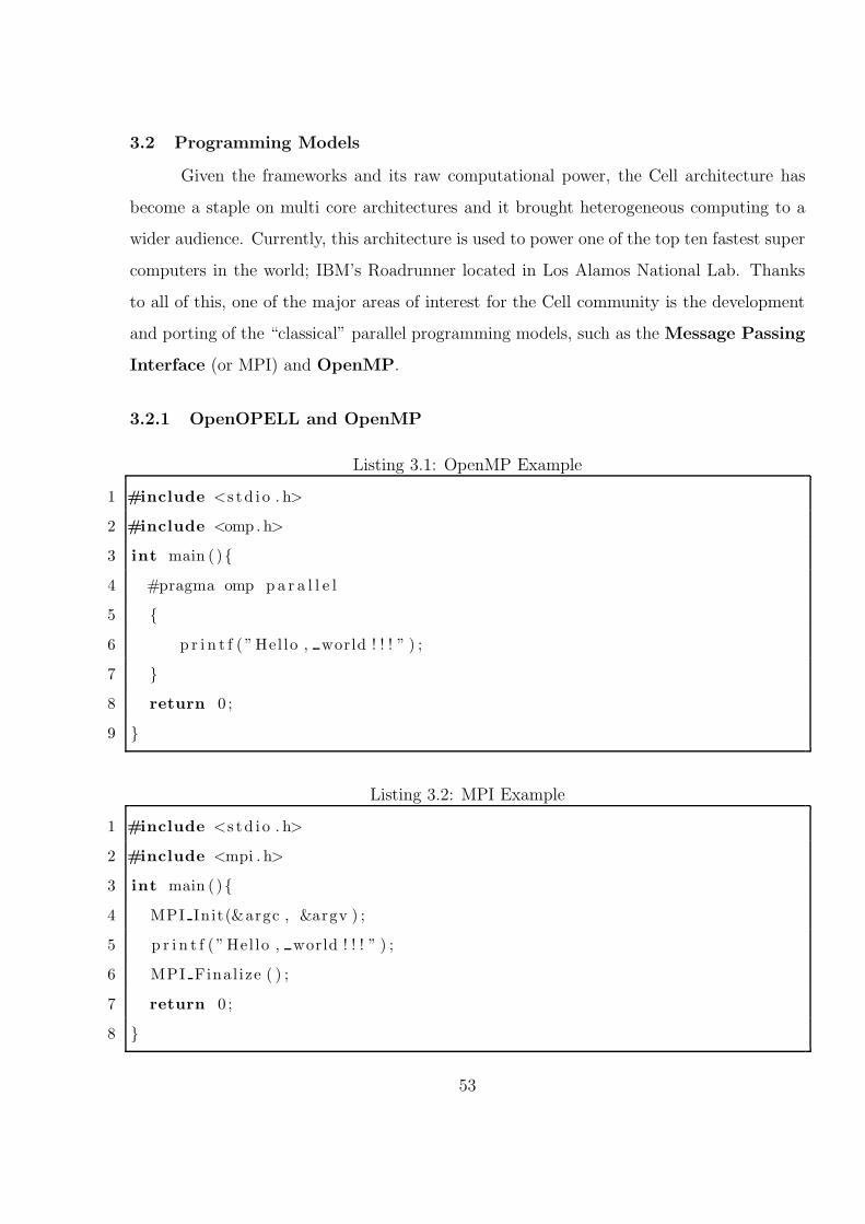
3.2 Programming Models
Given the frameworks and its raw computational power, the Cell architecture has
become a staple on multi core architectures and it brought heterogeneous computing to a
wider audience. Currently, this architecture is used to power one of the top ten fastest super
computers in the world; IBM’s Roadrunner located in Los Alamos National Lab. Thanks
to all of this, one of the major areas of interest for the Cell community is the development
and porting of the “classical” parallel programming models, such as the Message Passing
Interface (or MPI) and OpenMP.
3.2.1 OpenOPELL and OpenMP
Listing 3.1: OpenMP Example
1 #include <s td i o . h>
2 #include <omp . h>
3 int main ( ){
4 #pragma omp p a r a l l e l
5 {
6 p r i n t f ( ”Hel lo , world ! ! ! ” ) ;
7 }
8 return 0 ;
9 }
Listing 3.2: MPI Example
1 #include <s td i o . h>
2 #include <mpi . h>
3 int main ( ){
4 MPI Init(&argc , &argv ) ;
5 p r i n t f ( ”Hel lo , world ! ! ! ” ) ;
6 MPI Final ize ( ) ;
7 return 0 ;
8 }
53
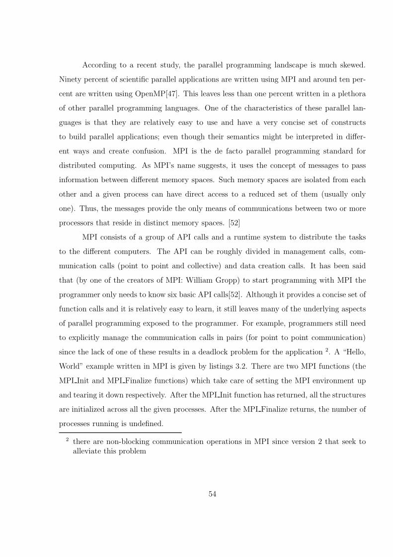
According to a recent study, the parallel programming landscape is much skewed.
Ninety percent of scientific parallel applications are written using MPI and around ten per-
cent are written using OpenMP[47]. This leaves less than one percent written in a plethora
of other parallel programming languages. One of the characteristics of these parallel lan-
guages is that they are relatively easy to use and have a very concise set of constructs
to build parallel applications; even though their semantics might be interpreted in differ-
ent ways and create confusion. MPI is the de facto parallel programming standard for
distributed computing. As MPI’s name suggests, it uses the concept of messages to pass
information between different memory spaces. Such memory spaces are isolated from each
other and a given process can have direct access to a reduced set of them (usually only
one). Thus, the messages provide the only means of communications between two or more
processors that reside in distinct memory spaces. [52]
MPI consists of a group of API calls and a runtime system to distribute the tasks
to the different computers. The API can be roughly divided in management calls, com-
munication calls (point to point and collective) and data creation calls. It has been said
that (by one of the creators of MPI: William Gropp) to start programming with MPI the
programmer only needs to know six basic API calls[52]. Although it provides a concise set of
function calls and it is relatively easy to learn, it still leaves many of the underlying aspects
of parallel programming exposed to the programmer. For example, programmers still need
to explicitly manage the communication calls in pairs (for point to point communication)
since the lack of one of these results in a deadlock problem for the application 2. A “Hello,
World” example written in MPI is given by listings 3.2. There are two MPI functions (the
MPI Init and MPI Finalize functions) which take care of setting the MPI environment up
and tearing it down respectively. After the MPI Init function has returned, all the structures
are initialized across all the given processes. After the MPI Finalize returns, the number of
processes running is undefined.
2 there are non-blocking communication operations in MPI since version 2 that seek toalleviate this problem
54
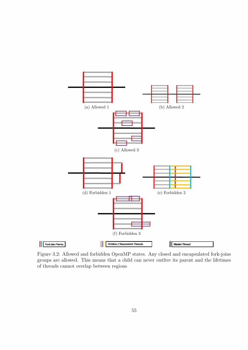
(a) Allowed 1 (b) Allowed 2
(c) Allowed 3
(d) Forbidden 1 (e) Forbidden 2
(f) Forbidden 3
Figure 3.2: Allowed and forbidden OpenMP states. Any closed and encapsulated fork-joinsgroups are allowed. This means that a child can never outlive its parent and the lifetimesof threads cannot overlap between regions
55
Conversely, OpenMP is used for architectures in which all the memory space is
(logically) visible to all processors. OpenMP is based on the fork-join computational model.
A master thread will “fork” a set of children threads and work with them up to a “join”
point in the future. No children (or any descendant of the master thread) will continue after
the join point. Moreover, no fork and join group are allowed to overlap unless one is from
a children of the fork and join group and it is completely enclosed by the outer fork-join
group. For a graphical representation of allowed and forbidden behaviors, please refer to
figure 3.2.
OpenMP is available for C, C++ and FORTRAN. It consists of several pragmas and
runtime function calls which are designed to support Single Program Multiple Data style of
programming, work sharing, synchronization between processors (both mutual exclusion and
ordering based) and task creation and management[1]. Due to its pragma based approach,
a serial code requires little change to make it run in parallel, as shown in example3.1 3.
Although OpenMP has been praised for its simplicity, it has been also criticized for it.
It provides little control over scheduling and work distribution which might create very
unbalanced workloads and a noticeable decrease in performance. It also has been accused
for being error prone due to some confusing constructs, i.e. flush, the lock function calls,
lastprivate variables, etc[2]. However, due to its popularity, OpenMP is a prime target for
porting across all the multi / many core architectures.
One of these project is the Open Source OpenMP on CELL (or Open OPELL for
short) developed at the University of Delaware [68]. Its main objective is to provide an open
source OpenMP framework for the Cell B.E. architecture. It is composed of an OpenMP
toolchain which produces Cell B.E. code from a single OpenMP source tree; and a runtime
that hides the heterogeneity of the architecture from the users. The framework provides
the following features: a single source compiler, software cache, partition / overlay manager
and a simple micro kernel.
3 However, to achieve high performance, a considerable amount of re-writing might benecessary
56
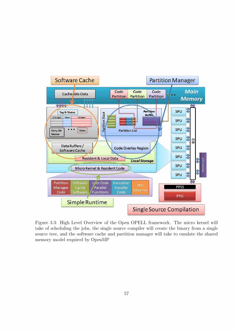
Figure 3.3: High Level Overview of the Open OPELL framework. The micro kernel willtake of scheduling the jobs, the single source compiler will create the binary from a singlesource tree, and the software cache and partition manager will take to emulate the sharedmemory model required by OpenMP
57
3.2.1.1 Single Source Compilation
Due to the heterogeneity of the Cell B.E., two distinct toolchains are needed to
compile code for the architecture. This adds more complications to an already complex
programming environment. In OPELL, the OpenMP source code is read by the driver
program. The driver clones the OpenMP source for both toolchains and calls the respective
compiler to do the work. The PPU compiler continues as expected even creating a copy of
the parallel function (which is the body of the parallel region in OpenMP) and inserting
the appropriate OpenMP runtime function calls when needed. The SPU compiler has a
different set of jobs. First, it keeps the parallel functions and discards the serial part of the
source code. Second, it inserts calls to the SPU execution handler (described in the next
section) and its framework to handle the parallel calls and OpenMP runtime calls. Third,
it inserts any extra function calls necessary to keep the semantics of the program. Finally,
it creates any structures needed for the other components of the runtime system, links the
correct libraries and generates the binary. After this step is completed, the control returns
to the driver which merges both executables into a single one. Figure 3.4 shows a high level
graphical overview of the whole single source process.
3.2.1.2 Simple Execution Handler
This small piece of code4 deals with the communication between the PPU and SPU
during runtime and how runtime and parallel function calls are handled. Since each of the
SPUs have very limited memory, it is in everybody’s best interest to keep the SPU threads
very light. To achieve this, the SPU thread will be loaded only with a minimal set of the
code (the simple execution handler and a set of libraries). This SPU resident code does
not include the parallel regions of the OpenMP code nor the OpenMP runtime libraries.
Since both are needed during runtime, they are both loaded or executed on demand, but by
different mechanisms. The parallel regions are loaded and executed by another component,
i.e. the partition manager, which loads and overlays code transparently. The OpenMP
4 In this thesis, the terms “simple execution handler” and “SPU micro kernel” will beused interchangeably
58
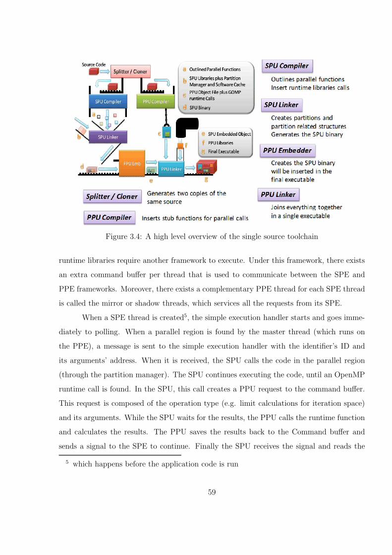
Figure 3.4: A high level overview of the single source toolchain
runtime libraries require another framework to execute. Under this framework, there exists
an extra command buffer per thread that is used to communicate between the SPE and
PPE frameworks. Moreover, there exists a complementary PPE thread for each SPE thread
is called the mirror or shadow threads, which services all the requests from its SPE.
When a SPE thread is created5, the simple execution handler starts and goes imme-
diately to polling. When a parallel region is found by the master thread (which runs on
the PPE), a message is sent to the simple execution handler with the identifier’s ID and
its arguments’ address. When it is received, the SPU calls the code in the parallel region
(through the partition manager). The SPU continues executing the code, until an OpenMP
runtime call is found. In the SPU, this call creates a PPU request to the command buffer.
This request is composed of the operation type (e.g. limit calculations for iteration space)
and its arguments. While the SPU waits for the results, the PPU calls the runtime function
and calculates the results. The PPU saves the results back to the Command buffer and
sends a signal to the SPE to continue. Finally the SPU receives the signal and reads the
5 which happens before the application code is run
59
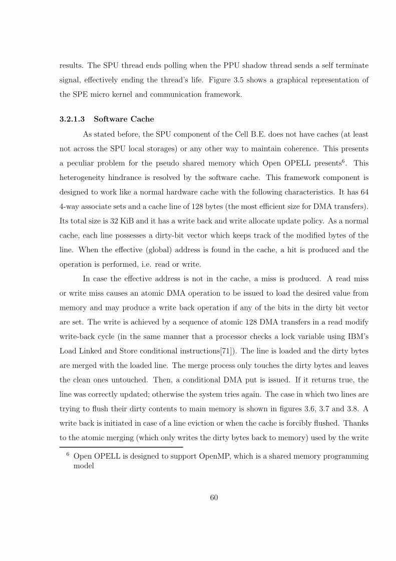
results. The SPU thread ends polling when the PPU shadow thread sends a self terminate
signal, effectively ending the thread’s life. Figure 3.5 shows a graphical representation of
the SPE micro kernel and communication framework.
3.2.1.3 Software Cache
As stated before, the SPU component of the Cell B.E. does not have caches (at least
not across the SPU local storages) or any other way to maintain coherence. This presents
a peculiar problem for the pseudo shared memory which Open OPELL presents6. This
heterogeneity hindrance is resolved by the software cache. This framework component is
designed to work like a normal hardware cache with the following characteristics. It has 64
4-way associate sets and a cache line of 128 bytes (the most efficient size for DMA transfers).
Its total size is 32 KiB and it has a write back and write allocate update policy. As a normal
cache, each line possesses a dirty-bit vector which keeps track of the modified bytes of the
line. When the effective (global) address is found in the cache, a hit is produced and the
operation is performed, i.e. read or write.
In case the effective address is not in the cache, a miss is produced. A read miss
or write miss causes an atomic DMA operation to be issued to load the desired value from
memory and may produce a write back operation if any of the bits in the dirty bit vector
are set. The write is achieved by a sequence of atomic 128 DMA transfers in a read modify
write-back cycle (in the same manner that a processor checks a lock variable using IBM’s
Load Linked and Store conditional instructions[71]). The line is loaded and the dirty bytes
are merged with the loaded line. The merge process only touches the dirty bytes and leaves
the clean ones untouched. Then, a conditional DMA put is issued. If it returns true, the
line was correctly updated; otherwise the system tries again. The case in which two lines are
trying to flush their dirty contents to main memory is shown in figures 3.6, 3.7 and 3.8. A
write back is initiated in case of a line eviction or when the cache is forcibly flushed. Thanks
to the atomic merging (which only writes the dirty bytes back to memory) used by the write
6 Open OPELL is designed to support OpenMP, which is a shared memory programmingmodel
60
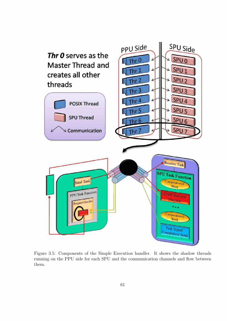
Figure 3.5: Components of the Simple Execution handler. It shows the shadow threadsrunning on the PPU side for each SPU and the communication channels and flow betweenthem.
61
back procedure certain problems, like the multiple writers and false sharing, can be avoided.
Currently, this component is being used to test the impact of weaker memory models on
multiprocessor architecture. A graphical overview of the software cache is presented by
figure 3.9.
Figure 3.6: Software Cache Merge Example Step 1: Before Write Back is Initialized
3.2.1.4 Overlay / Partition Manager
In the same manner that the software cache is used for data, the partition manager
is used for code. This small component is designed to load code on demand and manage
the code overlay space when needed. When compiling the source code, certain functions are
selected to be partitioned (not loaded with the original source code in the SPU memory).
The criteria to select these functions are based on the Function Call Graph, their size and
their runtime purpose, e.g. like parallel regions in OpenMP. Finally, the partitions are
created by the linker, descriptive structures are formed and special calling code is inserted
when appropriate. During runtime, the function call proceeds as usual (i.e. save registers,
62
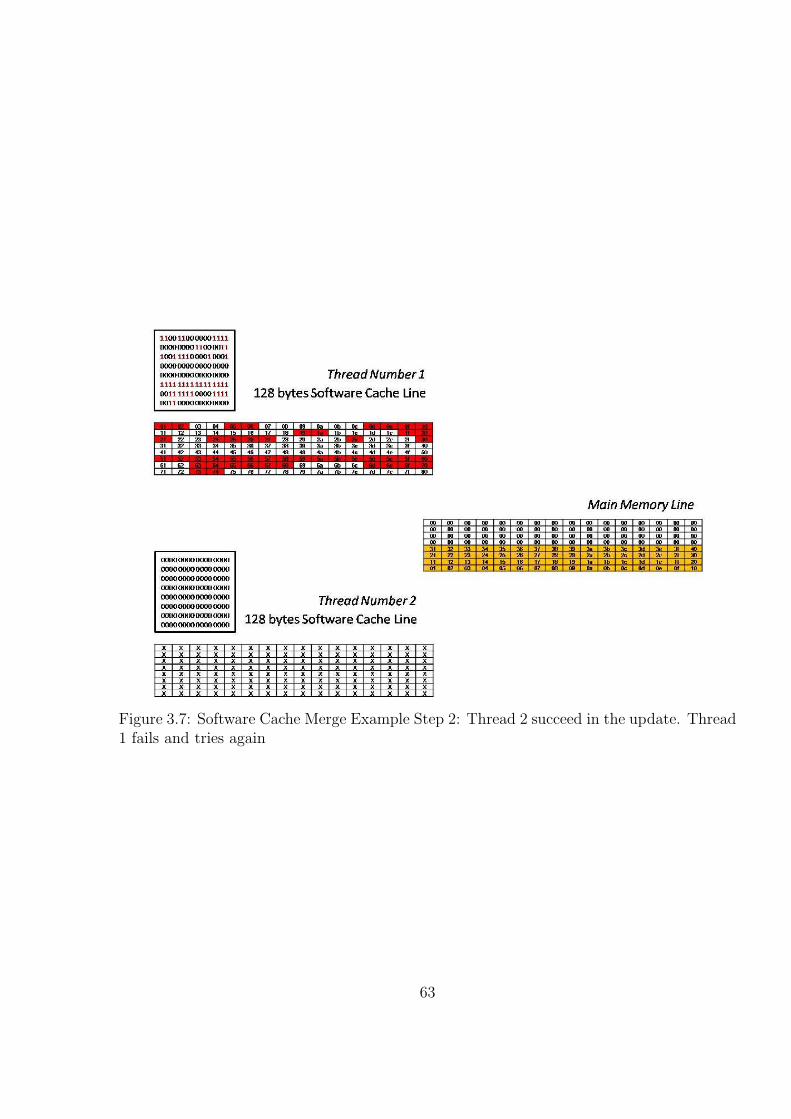
Figure 3.7: Software Cache Merge Example Step 2: Thread 2 succeed in the update. Thread1 fails and tries again
63
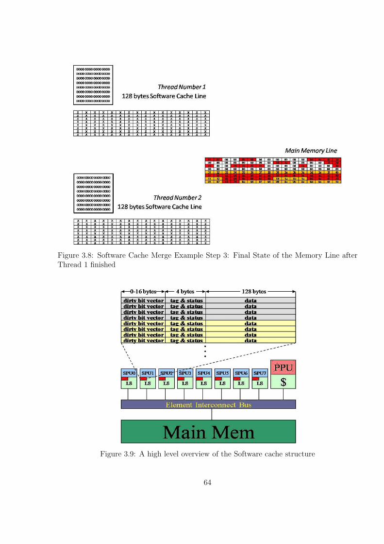
Figure 3.8: Software Cache Merge Example Step 3: Final State of the Memory Line afterThread 1 finished
Figure 3.9: A high level overview of the Software cache structure
64
load parameters, etc), up to the point of the actual call. Instead of jumping to the function,
the control is given to the partition manager runtime and several decoding steps are done
(which will be explored in Chapter 4). With information extracted from the actual symbol
address, a loading decision is made and the code is loaded into memory or not (if the code
already resides in the overlay). Then, the partition manager runtime passes control to the
function. When the function finishes, the control returns to the partition manager so any
cleaning task can be performed, like loading the caller partition if it was previously evicted.
Finally, the partition manager returns to its caller without leaving any trace of its
activities. For a more detailed explanation of the partition manager runtime, its enhance-
ments and replacement policies, please refer to Chapters 4 and 5. This thesis concentrates
on the partition manager component and its ability to support many performance enhancing
methods. The rest of this thesis will discuss the partition manager framework in detail.
65
Chapter 4
PARTITION MANAGER FRAMEWORK
The partition manager framework is designed to use both static analysis and dynamic
techniques to optimize the load and replacement of pieces of code. Changes in the toolchain
includes several switches to turn on and off the different partitioning schemes, a simple
partition algorithm and the creation of new segment types for the loader. The initial
framework consists of a simple trampoline that manages the overlay buffers and make sure
that the code is loaded in the correct places at the correct times. Next we explore the
changes that were made to the toolchain to support the dynamic nature of the partitions.
4.1 Toolchain Modifications
Although this thesis concentrates on partitioning schemes and its framework, an
overview of the components that makes this possible is in order. The changes on the tool
chain were not implemented by the author of this thesis 1 but he participated in the design
for all these components. This section covers, in a high level, the most significant changes
done to the GCC compiler, and the assembler and the linker from binutils version 2.18. A
high level overview of the role of each of the toolchain components is illustrated by Figure 4.1.
As seen in this figure, the compiler analyzes the code and create the partition by inserting
the necessary labels and directives. Next, the assembler generates the necessary code for the
partition and translate the directives into their correct machine code equivalent. Finally,
the linker assigns partition identification numbers to each partition, gather each partition
under a single executable and create the partition list.
1 Except for the changes that deals with the creation of the partition graph
66
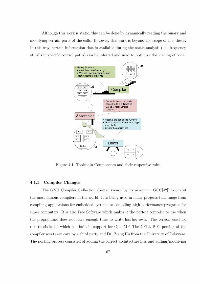
Although this work is static, this can be done by dynamically reading the binary and
modifying certain parts of the calls. However, this work is beyond the scope of this thesis.
In this way, certain information that is available during the static analysis (i.e. frequency
of calls in specific control paths) can be inferred and used to optimize the loading of code.
Figure 4.1: Toolchain Components and their respective roles
4.1.1 Compiler Changes
The GNU Compiler Collection (better known by its acronym: GCC[42]) is one of
the most famous compilers in the world. It is being used in many projects that range from
compiling applications for embedded systems to compiling high performance programs for
super computers. It is also Free Software which makes it the perfect compiler to use when
the programmer does not have enough time to write his/her own. The version used for
this thesis is 4.2 which has built-in support for OpenMP. The CELL B.E. porting of the
compiler was taken care by a third party and Dr. Ziang Hu from the University of Delaware.
The porting process consisted of adding the correct architecture files and adding/modifying
67
other files such that the SPE and PPE architectures are recognized and the correct code
is produced. Aside from the normal porting process, extra features were added so that
code partitioning can be supported. These features can be divided into three categories:
command line arguments, pragma directives and code partitioning algorithms (implemented
inside the compiler). The first two are explicitly presented to the programmers. The final
feature is implemented in the internals of the compiler. This dictates the way that code
is divided given the options provided by the former two. All three features are further
discussed below.
4.1.1.1 Command Line Flags
Command line flags are used to turn on and off certain compiler features. In our case,
these flags control the partition behavior, the algorithm used and the maximum number of
instructions per partition. The first command line flag is the -fcode-partition. This option
tells the compiler that the code being compiled needs to be divided into partitions using
the compiler’s internal algorithms. In this mode, the compiler ignores the pragmas that
the user added to the source code. The next flag is -fcode-partition-manu. This flags turns
off the compiler algorithms and uses the user pragmas to do the partitioning. Finally, the
–param max-partition-insns=n limits the number of instructions per partition to n or less.
4.1.1.2 Pragma Directives
Two pragma directives have been added to the preprocessor. These pragmas are
used to control the code partitioning when the -fcode-partition-manu flag is in effect. The
first directive is #pragma partitions x funcname1, funcname2, . . . , funcnamen. This
directive tells the compiler that the functions funcname1, funcname2 all the way up to
funcnamen reside in partition x. The x parameter defines a distinct partition but it will
not necessarily be the actual partition identification number which is assigned by the linker.
You can imagine, the parameter x being the logical partition number and the assigned
linker id the partition’s physical one. If a function is not present in any of the partitioning
pragmas, it is assigned to the default partition (which always resides in memory and is given
the identification number zero).
68
The final directive is #pragma keep function funcname1, funcname2, . . . ,
funcnamen. This pragma tells the compiler that functions funcname1, funcname2, up
to funcnamen need special attention when compiling. Usually, these functions reside in
different source files and that is why this directive flags them as special. As stated before, if
the compiler flag -fcode-partition is in effect, all these macros are ignored. A code example
can be seen in listing 4.1. In this example, the pragma in line 1 selects the main and the
bar functions to reside in partition zero and the pragma in line 2 puts the function foo in
partition 1.
As a final note, in all C code examples, the main function prototype is defined as
having an extra parameter, the spuid, which contains the runtime identification number of
the running SPE. The other two arguments in this function prototype represent a pointer
to the function arguments and a pointer to the environment parameters, respectively (both
located in the global memory)2.
Listing 4.1: Pragma Directives Example
1 #pragma p a r t i t i o n 0 main bar
2 #pragma p a r t i t i o n 1 foo
3 #include <s td i o . h>
4 void f oo (void ){}
5 void bar (void ){}
6 typedef unsigned long long ea t ;
7 int main ( ea t spuid , e a t argp , e a t envp ){
8 foo ( ) ;
9 bar ( ) ;
10 return 0 ;
11 }
2 Since the arguments resides outside the SPE local storage, a 64 bit pointer is passedto the SPE to locate the arguments. The void pointer cannot be used to pass thesearguments since in the SPE, this type represents four bytes (32 bits) instead of eight(64 bits)
69
4.1.1.3 Compiler Internals
When partitioning is enabled (either by adding -fcode-partition, or -fcode-partition-
manu), the compiler calls its partitioning function. This function behaves in two different
ways according to the options passed to it (either by the command line arguments and /
or by the directives). If manual partitioning is enabled, it collects the functions and groups
them into partitions based on the pragmas that it finds. In case that the generated partition,
created by either method is greater than the side of the allocated partition memory, the
runtime prevents its loading and gracefully quits.
If automatic partitioning is enabled, it goes through several steps. In the first step,
it creates a partition for each function. Next, it approximates the times that a given code
runs. This is done based on the number of basic blocks that each function has and if they
are in a loop or not. In this way, the cost matrix is created. The cost matrix a square matrix
that have as many rows as functions have been declared in the program. Elements in this
matrix represent how costly (based on the basic block estimated runtime information) is to
call a descendant partition.
Next the elements of the cost matrix are merged according to their costs. Let say we
have an element i which calls element j with a cost x. In case that the size of i + the size of
j is less than a specified threshold (e.g. maximum size of a partition under the framework)
and the cost x is the largest in that row, the rows i and j are merged. Under this process,
two complete rows are merged and one of them, plus its corresponding column, are deleted
from the matrix. When two rows are merged, the children’s costs and the rows’ sizes are
added. This process continues until the algorithm have exhausted all the children and/or
the maximum threshold has been met for each row. This ensures that the number of inter
partition calls are minimized.
After the compiler has finished creating the partitions, it generates assembly code.
When partitioning is enabled, the resulting code includes several assembly directives that
guides the assembler to produce correct machine code. These directives are inserted when
needed, as when calling a function in another partition; or to identify a section that holds
the partitioned code. Table 4.1 shows a list of the new assembly directives.
70
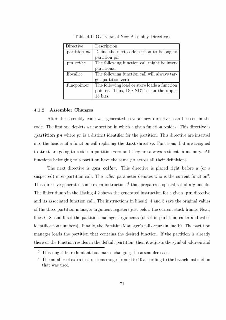
Table 4.1: Overview of New Assembly Directives
Directive Description.partition pn Define the next code section to belong to
partition pn.pm caller The following function call might be inter-
partitional.libcallee The following function call will always tar-
get partition zero.funcpointer The following load or store loads a function
pointer. Thus, DO NOT clean the upper15 bits.
4.1.2 Assembler Changes
After the assembly code was generated, several new directives can be seen in the
code. The first one depicts a new section in which a given function resides. This directive is
.partition pn where pn is a distinct identifier for the partition. This directive are inserted
into the header of a function call replacing the .text directive. Functions that are assigned
to .text are going to reside in partition zero and they are always resident in memory. All
functions belonging to a partition have the same pn across all their definitions.
The next directive is .pm caller . This directive is placed right before a (or a
suspected) inter-partition call. The caller parameter denotes who is the current function3.
This directive generates some extra instructions4 that prepares a special set of arguments.
The linker dump in the Listing 4.2 shows the generated instruction for a given .pm directive
and its associated function call. The instructions in lines 2, 4 and 5 save the original values
of the three partition manager argument registers just below the current stack frame. Next,
lines 6, 8, and 9 set the partition manager arguments (offset in partition, caller and callee
identification numbers). Finally, the Partition Manager’s call occurs in line 10. The partition
manager loads the partition that contains the desired function. If the partition is already
there or the function resides in the default partition, then it adjusts the symbol address and
3 This might be redundant but makes changing the assembler easier4 The number of extra instructions ranges from 6 to 10 according to the branch instructionthat was used
71
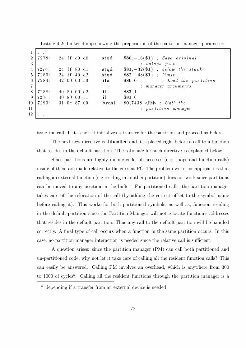
Listing 4.2: Linker dump showing the preparation of the partition manager parameters
1 . . .2 7278 : 24 f f c0 d0 stqd $80 ,−16($1 ) ; Save o r i g i n a l
3 ; v a l u e s j u s t
4 727 c : 24 f f 80 d1 stqd $81 ,−32($1 ) ; be low the s t a c k
5 7280: 24 f f 40 d2 stqd $82 ,−48($1 ) ; l i m i t
6 7284: 42 00 00 50 i l a $80 , 0 ; Load the p a r t i t i o n
7 ; manager arguments
8 7288: 40 80 00 d2 i l $82 , 19 728 c : 40 80 00 51 i l $81 , 0
10 7290: 31 0e 87 00 brasl $0 , 7438 <PM> ; Ca l l the
11 ; p a r t i t i o n manager
12 . . .
issue the call. If it is not, it initializes a transfer for the partition and proceed as before.
The next new directive is .libcallee and it is placed right before a call to a function
that resides in the default partition. The rationale for such directive is explained below.
Since partitions are highly mobile code, all accesses (e.g. loops and function calls)
inside of them are made relative to the current PC. The problem with this approach is that
calling an external function (e.g residing in another partition) does not work since partitions
can be moved to any position in the buffer. For partitioned calls, the partition manager
takes care of the relocation of the call (by adding the correct offset to the symbol name
before calling it). This works for both partitioned symbols, as well as, function residing
in the default partition since the Partition Manager will not relocate function’s addresses
that resides in the default partition. Thus any call to the default partition will be handled
correctly. A final type of call occurs when a function in the same partition occurs. In this
case, no partition manager interaction is needed since the relative call is sufficient.
A question arises: since the partition manager (PM) can call both partitioned and
un-partitioned code, why not let it take care of calling all the resident function calls? This
can easily be answered. Calling PM involves an overhead, which is anywhere from 300
to 1000 of cycles5. Calling all the resident functions through the partition manager is a
5 depending if a transfer from an external device is needed
72
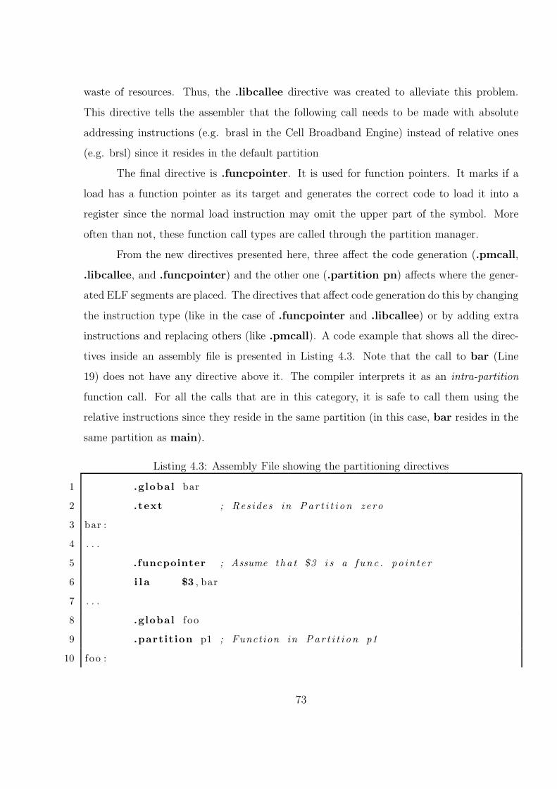
waste of resources. Thus, the .libcallee directive was created to alleviate this problem.
This directive tells the assembler that the following call needs to be made with absolute
addressing instructions (e.g. brasl in the Cell Broadband Engine) instead of relative ones
(e.g. brsl) since it resides in the default partition
The final directive is .funcpointer. It is used for function pointers. It marks if a
load has a function pointer as its target and generates the correct code to load it into a
register since the normal load instruction may omit the upper part of the symbol. More
often than not, these function call types are called through the partition manager.
From the new directives presented here, three affect the code generation (.pmcall,
.libcallee, and .funcpointer) and the other one (.partition pn) affects where the gener-
ated ELF segments are placed. The directives that affect code generation do this by changing
the instruction type (like in the case of .funcpointer and .libcallee) or by adding extra
instructions and replacing others (like .pmcall). A code example that shows all the direc-
tives inside an assembly file is presented in Listing 4.3. Note that the call to bar (Line
19) does not have any directive above it. The compiler interprets it as an intra-partition
function call. For all the calls that are in this category, it is safe to call them using the
relative instructions since they reside in the same partition (in this case, bar resides in the
same partition as main).
Listing 4.3: Assembly File showing the partitioning directives
1 .global bar
2 .text ; Resides in Par t i t i on zero
3 bar :
4 . . .
5 .funcpointer ; Assume tha t $3 i s a f unc . po in t e r
6 i l a $3 , bar
7 . . .
8 .global f oo
9 .partit ion p1 ; Function in Par t i t i on p1
10 foo :
73
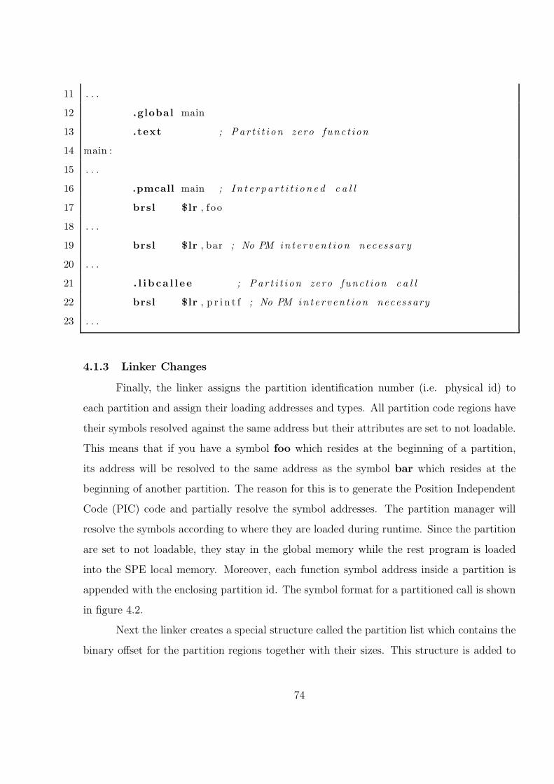
11 . . .
12 .global main
13 .text ; Par t i t i on zero func t i on
14 main :
15 . . .
16 .pmcall main ; I n t e r p a r t i t i o n e d c a l l
17 brsl $lr , f oo
18 . . .
19 brsl $lr , bar ; No PM in t e r v en t i on necessary
20 . . .
21 . l i b ca l l e e ; Par t i t i on zero func t i on c a l l
22 brsl $lr , p r i n t f ; No PM in t e r v en t i on necessary
23 . . .
4.1.3 Linker Changes
Finally, the linker assigns the partition identification number (i.e. physical id) to
each partition and assign their loading addresses and types. All partition code regions have
their symbols resolved against the same address but their attributes are set to not loadable.
This means that if you have a symbol foo which resides at the beginning of a partition,
its address will be resolved to the same address as the symbol bar which resides at the
beginning of another partition. The reason for this is to generate the Position Independent
Code (PIC) code and partially resolve the symbol addresses. The partition manager will
resolve the symbols according to where they are loaded during runtime. Since the partition
are set to not loadable, they stay in the global memory while the rest program is loaded
into the SPE local memory. Moreover, each function symbol address inside a partition is
appended with the enclosing partition id. The symbol format for a partitioned call is shown
in figure 4.2.
Next the linker creates a special structure called the partition list which contains the
binary offset for the partition regions together with their sizes. This structure is added to
74
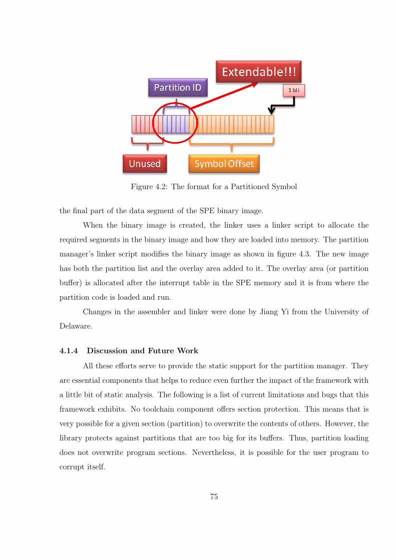
Figure 4.2: The format for a Partitioned Symbol
the final part of the data segment of the SPE binary image.
When the binary image is created, the linker uses a linker script to allocate the
required segments in the binary image and how they are loaded into memory. The partition
manager’s linker script modifies the binary image as shown in figure 4.3. The new image
has both the partition list and the overlay area added to it. The overlay area (or partition
buffer) is allocated after the interrupt table in the SPE memory and it is from where the
partition code is loaded and run.
Changes in the assembler and linker were done by Jiang Yi from the University of
Delaware.
4.1.4 Discussion and Future Work
All these efforts serve to provide the static support for the partition manager. They
are essential components that helps to reduce even further the impact of the framework with
a little bit of static analysis. The following is a list of current limitations and bugs that this
framework exhibits. No toolchain component offers section protection. This means that is
very possible for a given section (partition) to overwrite the contents of others. However, the
library protects against partitions that are too big for its buffers. Thus, partition loading
does not overwrite program sections. Nevertheless, it is possible for the user program to
corrupt itself.
75
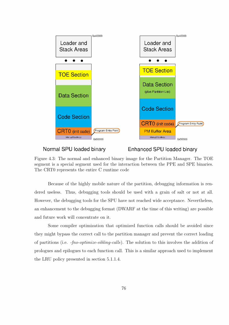
Figure 4.3: The normal and enhanced binary image for the Partition Manager. The TOEsegment is a special segment used for the interaction between the PPE and SPE binaries.The CRT0 represents the entire C runtime code
Because of the highly mobile nature of the partition, debugging information is ren-
dered useless. Thus, debugging tools should be used with a grain of salt or not at all.
However, the debugging tools for the SPU have not reached wide acceptance. Nevertheless,
an enhancement to the debugging format (DWARF at the time of this writing) are possible
and future work will concentrate on it.
Some compiler optimization that optimized function calls should be avoided since
they might bypass the correct call to the partition manager and prevent the correct loading
of partitions (i.e. -fno-optimize-sibling-calls). The solution to this involves the addition of
prologues and epilogues to each function call. This is a similar approach used to implement
the LRU policy presented in section 5.1.1.4.
76
These changes produces a binary that loads a stripped down program (without the
partitioned code) plus any necessary libraries (this includes the partition manager) into the
Cell’s SPE memory. The next chapter explains the partition manager, its extra structures
and its initial implementation.
4.2 Partition Manager and Its Framework
At the heart of the partitioning framework lies the partition manager. This function
is the one in charge of loading, correctly placing and, in general, managing the overlay space
and the partitions during runtime. The main difference between this small framework and
the GCC overlay framework is that it can manage the partitions dynamically, i.e. it can put
partitions anywhere in the overlay space. The idea behind the partition manager is similar to
the way that the instruction cache and the I-TLB works on super scalar architectures. Since
many-core architectures have these features reduced or eliminated, the partition manager
is an acceptable replacement for these methods. This chapter describes the ideas behind
the partition manager and their dynamic management of the overlay space. This section
concludes with the implementation of the partition manager on a many core architecture,
the Cell Broadband Engine. However, there is a certain terminology that needs to be
introduced in the next section.
4.2.1 Common Terminology
A function can have two types of states: temporary and permanent. The concept of
state under this framework is equivalent to registers. The permanent state of a function is
composed of the information that changes due to Partition manager interaction and must
be preserved across the function call. On the other hand, the temporary state is composed
of all the registers that are expected to be used by the calling function. If unsure this can
represent the entire register file. However, there are some guidelines that can be followed. If
all partition manager’s callees are known, the register usage can be found and an upper limit
of the number of registers to save can be calculated. Moreover, some scheduling “tricks”
can be used when writing the partition manager to reduce the number of used registers.
77
The difference between the temporary and permanent states is their lifetime. The
function’s permanent state needs to be saved across its lifetime. They are usually saved into
the partition related structure. On the other hand, the function’s temporary state needs
only to be saved and restored during certain areas of the partition manager code. Thus, the
space used for the temporary state can be reused across different partition manager calls.
The partition manager requires a small number of parameters passed to it. Moreover,
one of these parameters must be a callee saved so the function can be called. Please be
aware that two of the partition argument registers are considered temporary state and the
other one is considered permanent.
Next, a high level introduction to each partition manager and its components is
introduced.
4.2.2 The Partition Manager
The main objectives of the partition manager are to ensure that the correct function
is called and that the state is correctly passed between the different function calls. Given a
group of partitions, i.e. a code’s section which were created by the compiler as independent
“codelets”6. When a partioned function is called, the partition manager acts as a trampoline
between the caller and the callee. A trampoline under this framework is defined as a ghost
function which will do its work without leaving any visible traces of its activities. The
current framework depends on four structures. Some of them are created by the compiler,
while others are created and maintained during runtime. The major components of the
partition manager can be seen in Figure 4.4.
4.2.2.1 The Partition List
This structure is created by the toolchain, more specifically by its linker (explained
in 4.1). It consists of two parts which define the partition offset on the file and the partition
size. Moreover, the partition list resides in the computational element local memory; usually
just after the program’s data section. Under this framework, a partition is defined as a set
6 a function without unstructured gotos
78
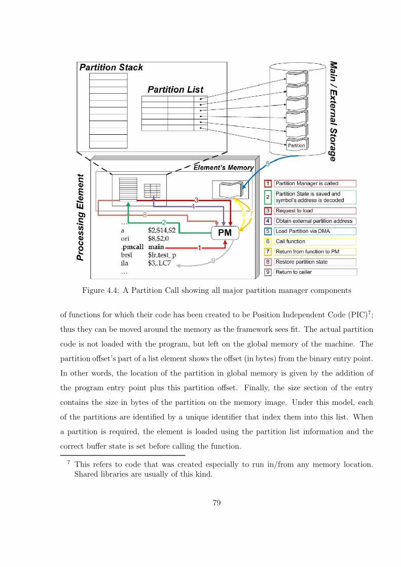
Figure 4.4: A Partition Call showing all major partition manager components
of functions for which their code has been created to be Position Independent Code (PIC)7;
thus they can be moved around the memory as the framework sees fit. The actual partition
code is not loaded with the program, but left on the global memory of the machine. The
partition offset’s part of a list element shows the offset (in bytes) from the binary entry point.
In other words, the location of the partition in global memory is given by the addition of
the program entry point plus this partition offset. Finally, the size section of the entry
contains the size in bytes of the partition on the memory image. Under this model, each
of the partitions are identified by a unique identifier that index them into this list. When
a partition is required, the element is loaded using the partition list information and the
correct buffer state is set before calling the function.
7 This refers to code that was created especially to run in/from any memory location.Shared libraries are usually of this kind.
79
4.2.2.2 The Partition Stack
The Partition Stack is a meta-structure which records the calling activity between
partitions. It was designed to solve a very simple problem: how to return from a function
call which was called from another partition?
By keeping the partition stack, the framework can know who was the parent of the
current function call, load the partition back if it is required and save the function state, i.e.
registers which must be saved across partition manager calls. Although the partition code is
defined as PIC, when returning from a function call, the framework must load the partition
back to its original position. If this is not the case then a large amount of binary rewriting
and register manipulation is needed to ensure the correct execution of the function. This
will result in a much greater overhead (almost linear with the size of the function) and a
more complex manager with several dependent structures (i.e. larger memory footprint).
4.2.2.3 The Partition Buffer
The Partition Buffer is a special region of the computational local memory, in which
the partition code is swap in and out. It is designed to have a fixed value per application,
but it can be divided into sub-buffers if required. The sub-buffers can help to take advan-
tage of certain program characteristics (i.e. locality, frequency of call, etc) to reduce the
communication between the main memory and the manager. Moreover, it contains certain
state, like the current Partition index and the lifetime of the code in this partition; which is
used for book-keeping and replacement policies as presented in chapter 5. Its management
is taken care by the partition manager. A special note, this buffer is not called a cache
because other policies besides cache-like can be applied to it.
4.2.2.4 The Partition Manager Kernel
At the center of all these structures lies the Partition Manager. This small function
handles the loading and management of the partitions in the system. During initialization,
the partition manager may statically divide the partition buffer so that several partitions
can co-exist with each other. It also applies a replacement policy to the buffers if required
(as discussed in chapter 5).
80
Although, the partition manager exists outside the programmers viewpoint, it still
requires some information to be passed to it. The partition manager has argument registers
which are restored before the partitioned call is invoked. However, at least one of these
argument register must be classified as callee saved register on the architectural ABI.
Finally, a description of the partition manager calling a function is described below.
4.2.2.5 The Anatomy of a Partitioned Call
When compiling a partitioned code, code generation occurs as expected down to
the assembly phase, i.e. arguments are prepared and code for function calls are inserted.
However, the assembler generates a slightly different code for a marked partition call site.
The saving and setting of the partition argument registers and the call to the partition
manager are inserted here. During runtime, when the partition manager is called, it saves
the function’s temporary state and checks its arguments. Second, the partition manager
pushes the current partition ID and the function’s permanent state to its partition stack.
Next, the manager checks if the current call needs to be loaded or if it already resides in the
local memory by checking the partition indexes that reside in the partition buffer against
the partition index of the function call. There can be three types of calls. The first type
involves functions which do not reside in the partition buffer because they were loaded with
the binary image at the beginning. These functions have the partition index of zero and no
dynamic relocation is made on them. The second type of function call is when the function
is already present in the partition buffer. In this case, the relocation is made by adding the
dynamic entry point of the buffer to the function address. Finally, the third case is when
the function is in a partition but it does not exit in the partition buffer. In this case, the
relocation takes place as before, and a load is issued for the given partition.
After the given partition is found (either it was there or it was loaded) and the
partition buffer state is updated, the function state is restored and the function call is
invoked. The callee saved argument register is used to call the function. The rationale
behind this restriction is that the framework needs at least one free register to call the
function and that if the callee function uses this register, the function (according to the
81
ABI) saves and restores this register accordingly. When the function returns, the partition
manager continues its execution to ensure that the return path of the function is restored.
After saving the function’s temporary state, the partition manager pops up its stack and
compares the current partition index with the returning partition index. If they differ then
the correct partition must be loaded and the partition buffer state must be updated. After
the return address has been validated, the function state and all argument registers are
restored to their original values and the partition manager returns.
In this way, the partition function call behaves like a ghost trampoline which ensure
that the partitions are available in memory at any point in time.
4.2.3 Cell Implementation of the Partition Framework: Version 1
This section describes the changes required to implement the partitioning framework
under the Cell Broadband Engine. For the changes on the toolchain side, please refer to
4.1. The kernel of the partition manager was written in assembly to optimize register usage
and depends heavily on several structures which implements the framework components
described above. On this version, the partition buffer is not further subdivided so the
replacement policy is trivial.
4.2.3.1 Partition List Structures and Variables
The variables associated with the partition list component of the framework are de-
fined in the linker script that accompanies the toolchain or in the structure handle of the
binary image (provided by the spu handle t structure data type). The variables declared in
the linker script are the partition list and partition size which represent the address
and the size (in bytes) of the partition list. As mentioned before, these variables are ini-
tialized and loaded by the linker at the application linking time. The partition list location
are at the end of the data section of the new binary image and it has a maximum size of
512 bytes. Under this configuration, the framework can support up to thirty two distinct
partitions.
82
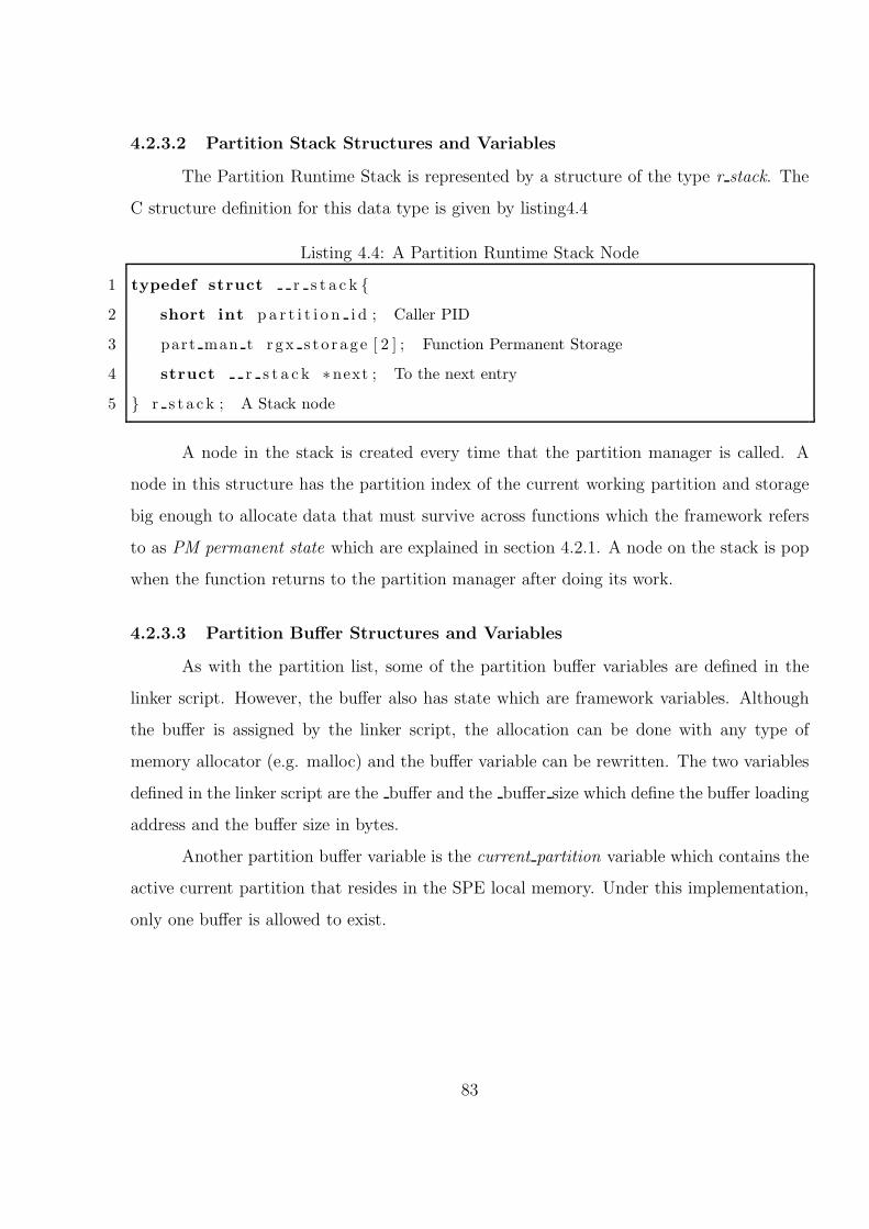
4.2.3.2 Partition Stack Structures and Variables
The Partition Runtime Stack is represented by a structure of the type r stack. The
C structure definition for this data type is given by listing4.4
Listing 4.4: A Partition Runtime Stack Node
1 typedef struct r s t a c k {
2 short int p a r t i t i o n i d ; Caller PID
3 part man t r gx s t o r age [ 2 ] ; Function Permanent Storage
4 struct r s t a c k ∗next ; To the next entry
5 } r s t a c k ; A Stack node
A node in the stack is created every time that the partition manager is called. A
node in this structure has the partition index of the current working partition and storage
big enough to allocate data that must survive across functions which the framework refers
to as PM permanent state which are explained in section 4.2.1. A node on the stack is pop
when the function returns to the partition manager after doing its work.
4.2.3.3 Partition Buffer Structures and Variables
As with the partition list, some of the partition buffer variables are defined in the
linker script. However, the buffer also has state which are framework variables. Although
the buffer is assigned by the linker script, the allocation can be done with any type of
memory allocator (e.g. malloc) and the buffer variable can be rewritten. The two variables
defined in the linker script are the buffer and the buffer size which define the buffer loading
address and the buffer size in bytes.
Another partition buffer variable is the current partition variable which contains the
active current partition that resides in the SPE local memory. Under this implementation,
only one buffer is allowed to exist.
83
4.2.3.4 Partition Manager Support Structures, Variables and Calling Proce-
dure
The partition manager uses all the variables mentioned before and add some of its
own to the framework. Under the CBE implementation, the function’s permanent state is
represented by two registers: the linkage register which contains the original return value of
the function and the partition argument register’s original values. This register is used to
call the function from the partition manager. As the partition manager does not change the
function stack in any visible way or the environment, the stack pointer and the environment
variable are not part of the function’s permanent state. On the other hand, the temporary
state is composed of all the registers that are expected to be used by the calling function.
In the initial versions of the framework, this represented the entire register file. However,
we used some tricks (besides smart scheduling) that are useful for reducing the size of the
temporary state.
To reduce the temporary state, the partition manager must know all the registers that
are used. Although this might seem trivial, the partition manager does not have any control
(or even knowledge) on the registers used in its library calls (i.e. memcpy, main memory
transfers, timing functions, print statements, etc). To overcome this obstacle, the Cholo
libraries were created. These libraries provide an API for common functions that deals with
memory copying and transferring, timing and software based interrupts. The advantages
of these libraries is that the PM writer knows all the registers that are used in them (since
he has access to the source code and object code) and can control their allocation. Most
of the functions in the Cholo library are based or copied (with minimal changes) from one
of the standard implementation of such functions8. Thanks to this extension, the size of
temporary state can be reduced from 1.25 Kilobytes to 352 bytes only. During a partition
manager call, only one temporary state can exists. The function’s temporary state is saved
in an array called the register storage.
An important point to make here is that since the function stack and the data
8 e.g. the memcpy in the Cholo libraries is based on its implementation in the GNU Clibrary with minimal changes.
84
segments resides in the same flat memory in the SPE memory and there is no penalty (or
benefit) to access the stack versus normal SPE memory, all the framework variables are
declared global so that the stack pointer is not modified. Finally, the original values of
the argument registers, which are defined to be the registers 80, 81 and 82 in the CBE
architecture, are saved just beyond the original function’s stack frame.
4.2.4 A Partitioned Call on CBE: Version 1
In the section 4.2.2.5, a high level overview of how a partitioned call is made was
presented. This subsection presents how a call is invoked when running on the CBE version
of the framework. Please note that this is the basic framework of the partition manager.
Advanced frameworks built upon this one are explained in section 5.
Before the partition manager is called, registers 80, 81 and 82 are filled with the
partition manager parameters. These register original contents are saved just below the
current stack frame. After the parameters have been prepared, the partition manager is
called. The manager saves the function’s temporary state which includes the original values
of 81 and 82 before doing anything else. Next, the partition identification number for the
new partition and the function address are decoded. When decoding the partition id, the
caller’s partition id plus the function’s permanent state (i.e. register 80 and the link register)
are pushed into the partition stack. In case that the callee’s partition id is zero or is the
same as the current partition id then decoding returns a value of zero, which means do not
load.
If a new partition needs to be loaded, then decoding returns the partition id of the
new partition and updates the current partition variable. The decoding for the function
symbol consists of adjustments made to the symbol address. As stated in section 4.1, the
symbol of a function that resides in a partition consists of the offset from its partition start
and its partition index on the upper seven bits. During symbol decoding, the buffer’s offset
is added to the symbol (i.e. offset) without the upper seven bits (which contains the symbol
partition’s index). This creates an absolute function pointer. However, if the symbol resides
in partition zero, nothing is added to it because the symbol address is assumed to be the
85
absolute address.
After the index is decoded, the partition is loaded. Afterwards, the transient state is
restored. The function is invoked using the register 809. This whole process is depicted by
the flowchart in figure 4.5. After the function returns, the transient/temporary state10 are
saved. At this point, the partition stack is popped. This loads register 80’s original value
and the link register with the original return address (back to the caller)11 in a temporary
holder. It also pops the partition id from the caller. Since the target of the link register
might be in a partition, the partition manager needs to check the partition index from
the caller against the current partition. If the indexes are not the same then a transfer is
issued to load the correct partition and update the current partition variable. After this,
the partition manager restores the transient and the permanent states for a final time and
returns. A flowchart of this process is given by figure 4.6
A major observation can be made. The partition buffer might be sub-divided so that
it can hold multiple partitions at the same time. In this way, several code features and
characteristics can be exploited to improve performance. An extension to this design is to
dynamically divide the buffer and then manage each of the sub-buffer as a distinct partition
buffer. This includes adding several variables to the framework and replacing policies on
the sub-buffers.
9 at this point, registers 81 and 82 have been restored already to their original values10 minus 81 and 8211 The last value that the link register had was inside the partition manager
86
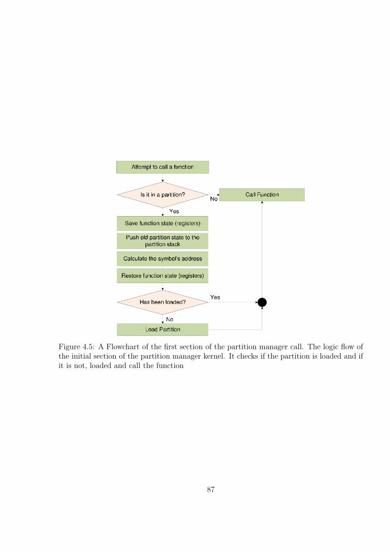
Figure 4.5: A Flowchart of the first section of the partition manager call. The logic flow ofthe initial section of the partition manager kernel. It checks if the partition is loaded and ifit is not, loaded and call the function
87
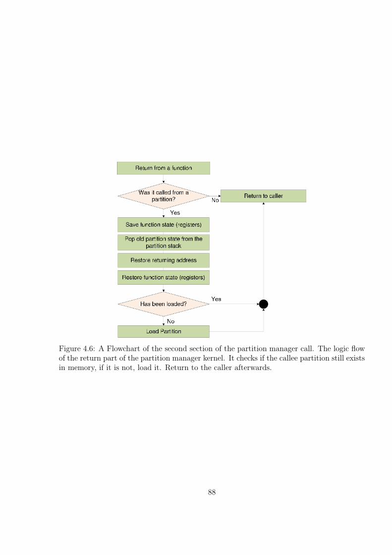
Figure 4.6: A Flowchart of the second section of the partition manager call. The logic flowof the return part of the partition manager kernel. It checks if the callee partition still existsin memory, if it is not, load it. Return to the caller afterwards.
88
Chapter 5
PARTITION MANAGER ENHANCEMENTS
In its original form, the partition manager wastes many opportunities to reduce the
number of long latency operations and the overlapping of computation and communication.
This chapter explores the advantages and disadvantages of certain classical hardware /
software optimization techniques when applied to the framework.
We continue to explore the partition manager space by dividing the overlay / buffer
space into different sub partitions and then applying several algorithms to reduce the number
of long latency operations in many scenarios (cache-like versus pre-fetching schemes versus
victim cache).
5.1 The N Buffer: The Lazy Reuse Approaches
All partition manager components were explained in the Chapter 4. However, as
observed in the last paragraph of that chapter, the partition buffer can be broken down into
sub-buffers. This opens many interesting possibilities on how to manage the sub-buffers to
increase performance. Even though this area is not new, these techniques are usually applied
in hardware. This chapter shows two hardware buffer management techniques applied to the
partitioning framework. The first one is the simplest one in which the buffer subdivisions
are treated as a FIFO (first in first out) structure. In this context, this technique is called
Modulus due to the operation used to select the next replacement. The second one is based
on one of the most famous (and successful) cache replacement policies: Least Recently Used
(LRU). This section describes both techniques and their implementation in the partition
manager framework. However, a look inside the N Buffer approach is in order.
89
5.1.1 The N Buffer Approach
Under this approach, the buffer is broken in N pieces and all of them are managed by
the partitioning framework. Since there are many sub-buffers to select from, a replacement
technique is placed into effect to better utilize the buffer space. This technique refers on
how to choose the next sub-buffer when a new partition needs to be loaded. Moreover, the
framework behaves slightly different when loading the partition. The framework can either
take advantage of reuse (lazily reusing the already loaded partitions) or actively loading
them into the buffers. In this section, we deal with lazy reuse techniques. However, the
framework is extensible enough to add other features if required. Before talking about the
techniques that we are using, we should take a look on how partitioning the partition buffer
affects the framework components.
5.1.1.1 The Partition Buffer
The partition buffer is affected by adding an extra state. Each sub-buffer must
contain the partition index residing inside of it and an extra integer value to help achieve
advanced replacement features (i.e. the integer can represent lifetime for LRU or the next
partition index on a pre-fetching mechanism). Moreover, the partition that resides in local
memory become stateful under this model. This means that instead of just being loaded
and not-loaded, now they can be active, in-active, evicted or evicted with the opportunity of
reuse. For a description of the new states and their meanings, please refer to table 5.1.
Every partition begins in the evicted state in the main memory. When a call to a
function in that partition is issued, the partition is loaded and becomes active. From this
state the partition can become in-active, if a new partition is needed and this one resides
into a sub-buffer which is not replaced; back to evicted, if it is replaced and it doesn’t belong
to the return path of a chain of partitioned function calls; or Evicted with an Opportunity
to Reuse, in the case that a partition is kicked out but it lies on the return path of a chain
of partitioned function calls. An in-active partition may transition to evicted and EWOR
under the same conditions as an active one. An EWOR partition can only transition to an
active partition or evicted if the application requires more memory (see 5.2.1).
90
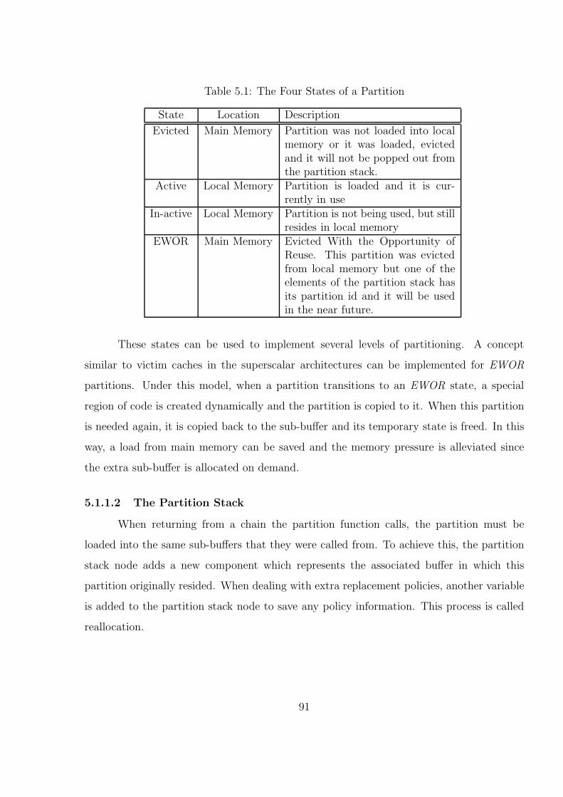
Table 5.1: The Four States of a Partition
State Location Description
Evicted Main Memory Partition was not loaded into localmemory or it was loaded, evictedand it will not be popped out fromthe partition stack.
Active Local Memory Partition is loaded and it is cur-rently in use
In-active Local Memory Partition is not being used, but stillresides in local memory
EWOR Main Memory Evicted With the Opportunity ofReuse. This partition was evictedfrom local memory but one of theelements of the partition stack hasits partition id and it will be usedin the near future.
These states can be used to implement several levels of partitioning. A concept
similar to victim caches in the superscalar architectures can be implemented for EWOR
partitions. Under this model, when a partition transitions to an EWOR state, a special
region of code is created dynamically and the partition is copied to it. When this partition
is needed again, it is copied back to the sub-buffer and its temporary state is freed. In this
way, a load from main memory can be saved and the memory pressure is alleviated since
the extra sub-buffer is allocated on demand.
5.1.1.2 The Partition Stack
When returning from a chain the partition function calls, the partition must be
loaded into the same sub-buffers that they were called from. To achieve this, the partition
stack node adds a new component which represents the associated buffer in which this
partition originally resided. When dealing with extra replacement policies, another variable
is added to the partition stack node to save any policy information. This process is called
reallocation.
91
5.1.1.3 The Modulus Method
The modulus method is the simplest one of the two lazy reuse methods. In this
method, the variable pointed to the next sub-buffer to be filled is updated using using a
First-In-First-Out (FIFO) policy. In this method, the oldest existing partition is always
replaced. The advantages of this method are that is very easy to implement since it only
requires a simple remainder (i.e. FIFO) operation to select the next sub-buffer. Moreover,
this method does surprisingly well in applications in which the code is not reused that often,
i.e. partitioned calls inside loops. Nevertheless, since it does not recognize reuse, a very
“hot”partition can be replaced before it is completely used. This might create many extra
transfers which represents anywhere from dozens to thousands of cycles lost. Because of
this, the next method takes in consideration reuse and with this information; it decides the
next sub-buffer that is replaced. An inter partitioned call using the modulus methods goes
as follows. Save the PM permanent and PM transient registers. Then decode the partition
id and the address. While decoding the partition id, push to the partition stack (together
with the caller’s sub-buffer id1) and decide if the partition needs to be loaded. If it needs
to, calculate the sub-buffer in FIFO order. Update the sub-buffer array, the next sub-buffer
variable and the current partition variables. When decoding the symbol, take the values of
the current sub buffer and the sub buffer size to ensure that the symbol address is pointing
to the correct sub-buffer. After this step, the loading of the new partition takes place. The
PM transient registers are restored and the symbol is called. After the function returns, the
PM transient2 are saved and the partition stack is popped. This puts the contents of the
PM permanent in a temporary holder. While the stack is being pop, the associated buffer
and the caller partition id are checked. If the partition is in memory and in its correct sub
buffer then no further action is needed. If the partition is still in memory, but not in the
correct sub-buffer, then the partition is copied to the correct sub buffer and the old sub
buffer is marked “available.”If the partition is not in local memory at all then it is loaded.
Finally, all registers are restored to their original contents and the function returns.
1 in the associated buffer variable2 sans 81 and 82
92
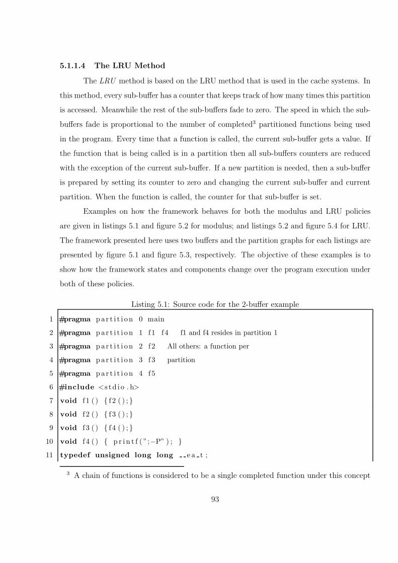
5.1.1.4 The LRU Method
The LRU method is based on the LRU method that is used in the cache systems. In
this method, every sub-buffer has a counter that keeps track of how many times this partition
is accessed. Meanwhile the rest of the sub-buffers fade to zero. The speed in which the sub-
buffers fade is proportional to the number of completed3 partitioned functions being used
in the program. Every time that a function is called, the current sub-buffer gets a value. If
the function that is being called is in a partition then all sub-buffers counters are reduced
with the exception of the current sub-buffer. If a new partition is needed, then a sub-buffer
is prepared by setting its counter to zero and changing the current sub-buffer and current
partition. When the function is called, the counter for that sub-buffer is set.
Examples on how the framework behaves for both the modulus and LRU policies
are given in listings 5.1 and figure 5.2 for modulus; and listings 5.2 and figure 5.4 for LRU.
The framework presented here uses two buffers and the partition graphs for each listings are
presented by figure 5.1 and figure 5.3, respectively. The objective of these examples is to
show how the framework states and components change over the program execution under
both of these policies.
Listing 5.1: Source code for the 2-buffer example
1 #pragma p a r t i t i o n 0 main
2 #pragma p a r t i t i o n 1 f 1 f 4 f1 and f4 resides in partition 1
3 #pragma p a r t i t i o n 2 f 2 All others: a function per
4 #pragma p a r t i t i o n 3 f 3 partition
5 #pragma p a r t i t i o n 4 f 5
6 #include <s td i o . h>
7 void f 1 ( ) { f 2 ( ) ; }
8 void f 2 ( ) { f 3 ( ) ; }
9 void f 3 ( ) { f 4 ( ) ; }
10 void f 4 ( ) { p r i n t f ( ”;−P” ) ; }
11 typedef unsigned long long e a t ;
3 A chain of functions is considered to be a single completed function under this concept
93
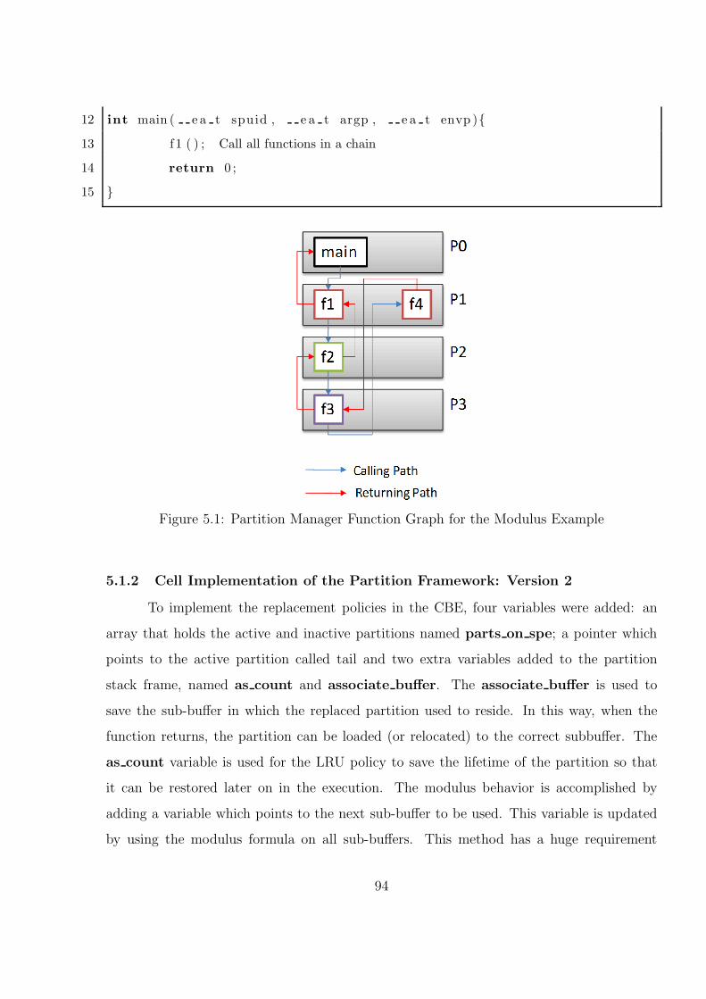
12 int main ( e a t spuid , e a t argp , e a t envp ){
13 f1 ( ) ; Call all functions in a chain
14 return 0 ;
15 }
Figure 5.1: Partition Manager Function Graph for the Modulus Example
5.1.2 Cell Implementation of the Partition Framework: Version 2
To implement the replacement policies in the CBE, four variables were added: an
array that holds the active and inactive partitions named parts on spe; a pointer which
points to the active partition called tail and two extra variables added to the partition
stack frame, named as count and associate buffer. The associate buffer is used to
save the sub-buffer in which the replaced partition used to reside. In this way, when the
function returns, the partition can be loaded (or relocated) to the correct subbuffer. The
as count variable is used for the LRU policy to save the lifetime of the partition so that
it can be restored later on in the execution. The modulus behavior is accomplished by
adding a variable which points to the next sub-buffer to be used. This variable is updated
by using the modulus formula on all sub-buffers. This method has a huge requirement
94
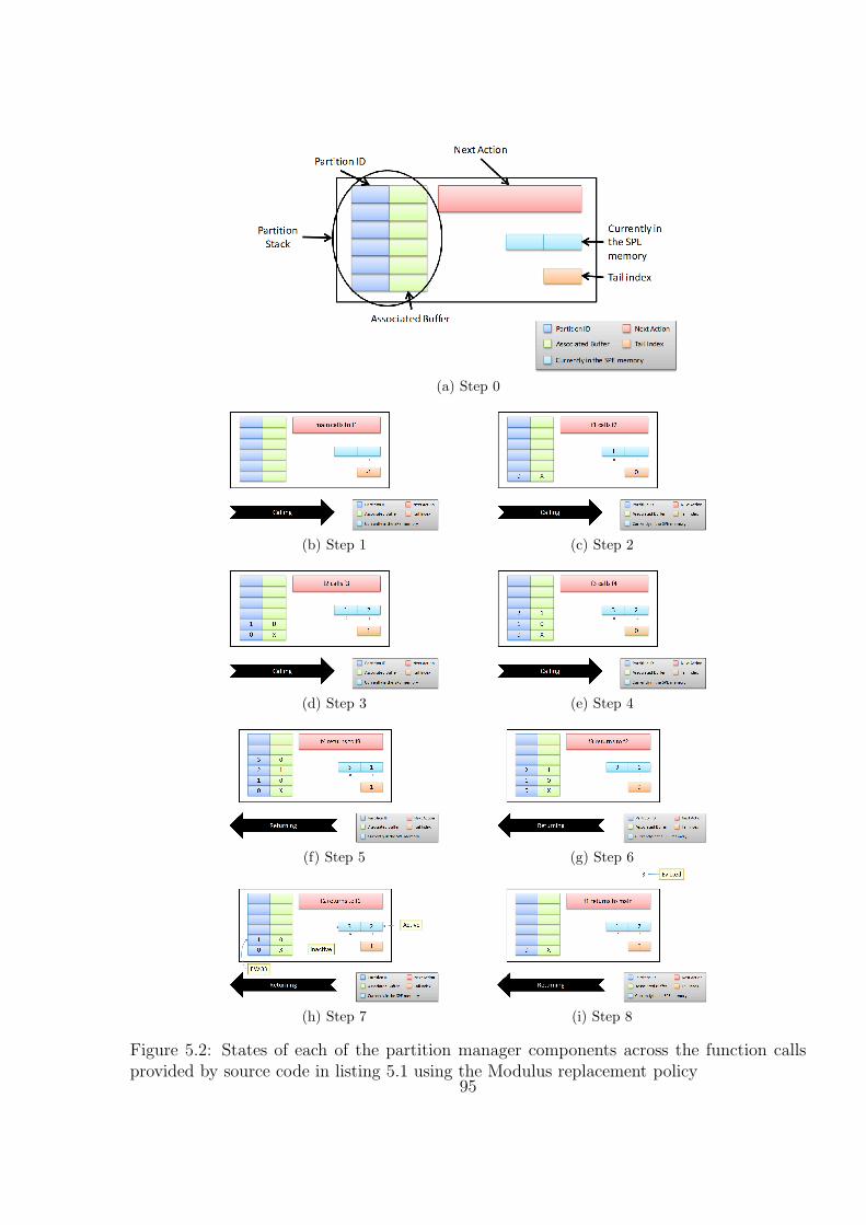
(a) Step 0
(b) Step 1 (c) Step 2
(d) Step 3 (e) Step 4
(f) Step 5 (g) Step 6
(h) Step 7 (i) Step 8
Figure 5.2: States of each of the partition manager components across the function callsprovided by source code in listing 5.1 using the Modulus replacement policy
95
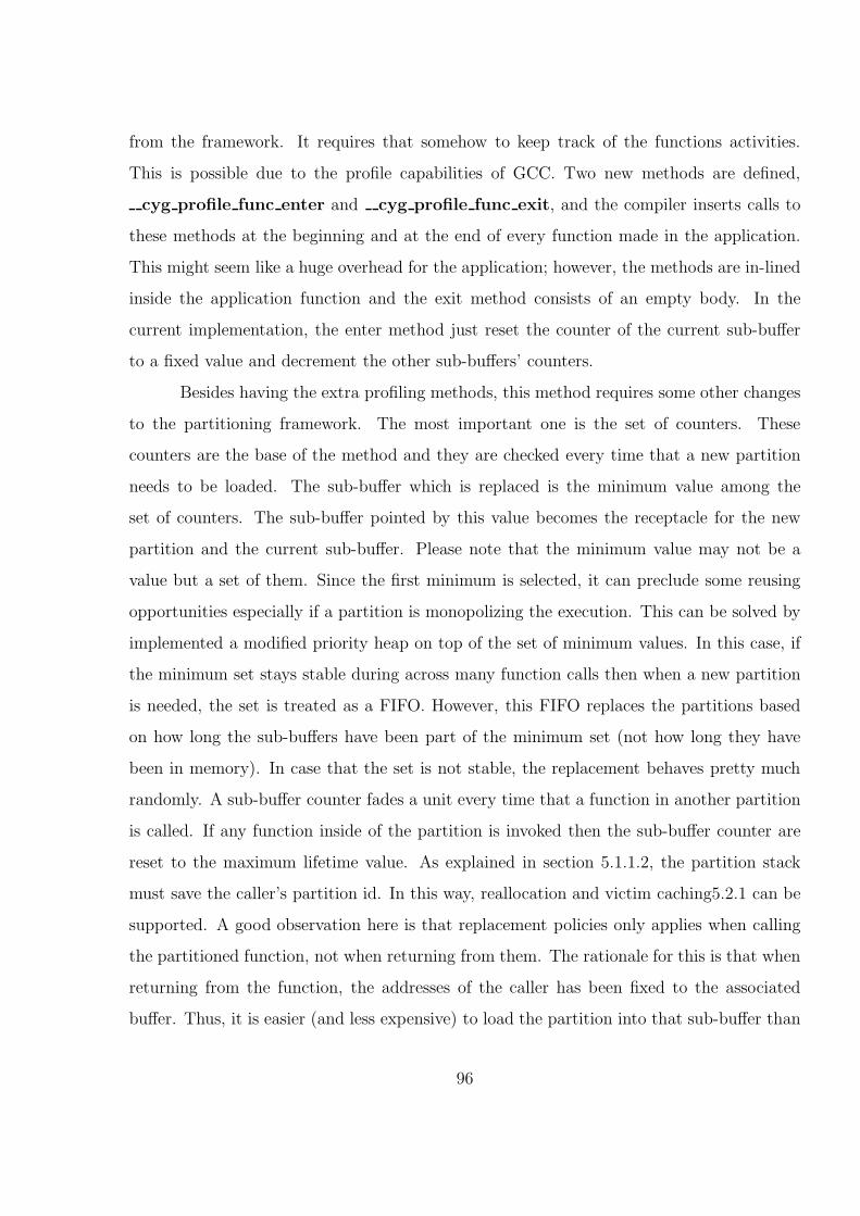
from the framework. It requires that somehow to keep track of the functions activities.
This is possible due to the profile capabilities of GCC. Two new methods are defined,
cyg profile func enter and cyg profile func exit, and the compiler inserts calls to
these methods at the beginning and at the end of every function made in the application.
This might seem like a huge overhead for the application; however, the methods are in-lined
inside the application function and the exit method consists of an empty body. In the
current implementation, the enter method just reset the counter of the current sub-buffer
to a fixed value and decrement the other sub-buffers’ counters.
Besides having the extra profiling methods, this method requires some other changes
to the partitioning framework. The most important one is the set of counters. These
counters are the base of the method and they are checked every time that a new partition
needs to be loaded. The sub-buffer which is replaced is the minimum value among the
set of counters. The sub-buffer pointed by this value becomes the receptacle for the new
partition and the current sub-buffer. Please note that the minimum value may not be a
value but a set of them. Since the first minimum is selected, it can preclude some reusing
opportunities especially if a partition is monopolizing the execution. This can be solved by
implemented a modified priority heap on top of the set of minimum values. In this case, if
the minimum set stays stable during across many function calls then when a new partition
is needed, the set is treated as a FIFO. However, this FIFO replaces the partitions based
on how long the sub-buffers have been part of the minimum set (not how long they have
been in memory). In case that the set is not stable, the replacement behaves pretty much
randomly. A sub-buffer counter fades a unit every time that a function in another partition
is called. If any function inside of the partition is invoked then the sub-buffer counter are
reset to the maximum lifetime value. As explained in section 5.1.1.2, the partition stack
must save the caller’s partition id. In this way, reallocation and victim caching5.2.1 can be
supported. A good observation here is that replacement policies only applies when calling
the partitioned function, not when returning from them. The rationale for this is that when
returning from the function, the addresses of the caller has been fixed to the associated
buffer. Thus, it is easier (and less expensive) to load the partition into that sub-buffer than
96
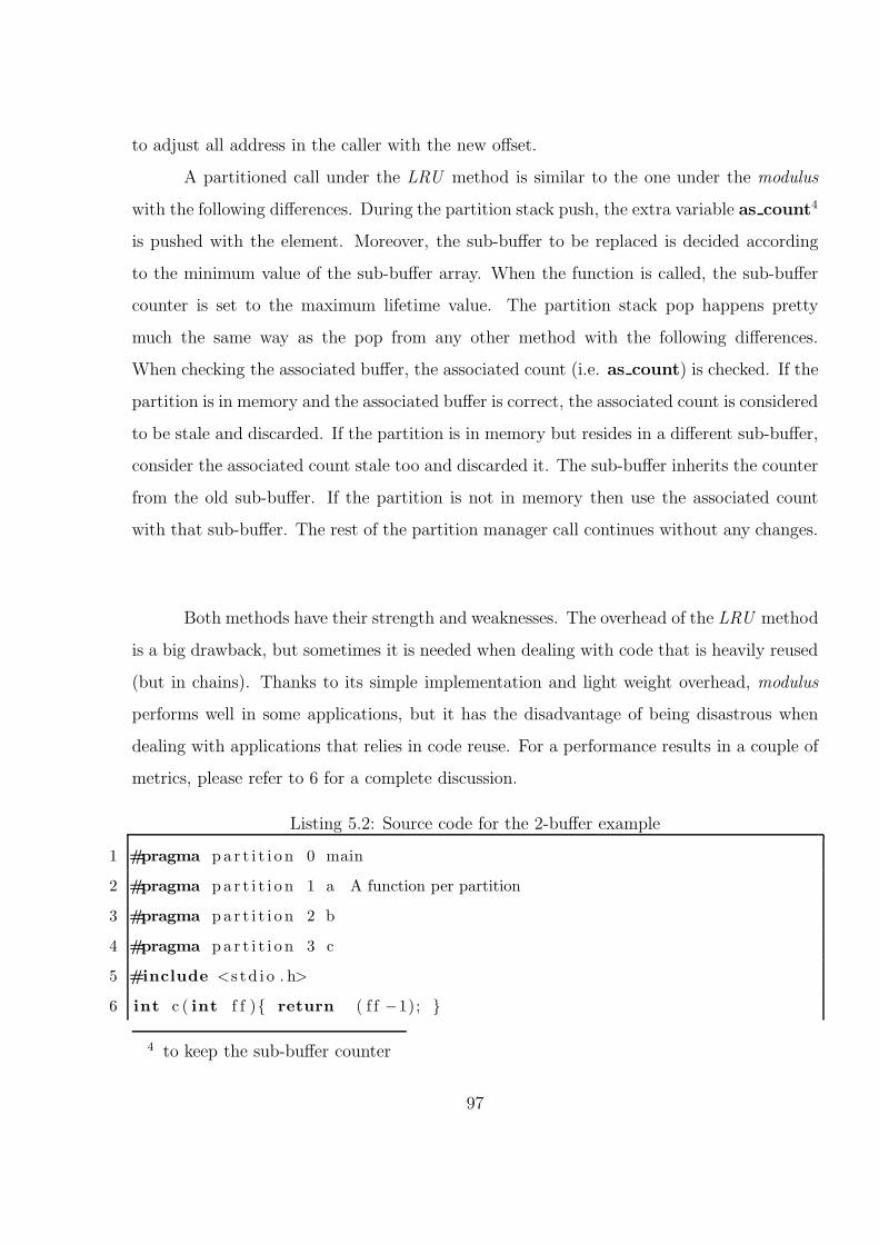
to adjust all address in the caller with the new offset.
A partitioned call under the LRU method is similar to the one under the modulus
with the following differences. During the partition stack push, the extra variable as count4
is pushed with the element. Moreover, the sub-buffer to be replaced is decided according
to the minimum value of the sub-buffer array. When the function is called, the sub-buffer
counter is set to the maximum lifetime value. The partition stack pop happens pretty
much the same way as the pop from any other method with the following differences.
When checking the associated buffer, the associated count (i.e. as count) is checked. If the
partition is in memory and the associated buffer is correct, the associated count is considered
to be stale and discarded. If the partition is in memory but resides in a different sub-buffer,
consider the associated count stale too and discarded it. The sub-buffer inherits the counter
from the old sub-buffer. If the partition is not in memory then use the associated count
with that sub-buffer. The rest of the partition manager call continues without any changes.
Both methods have their strength and weaknesses. The overhead of the LRU method
is a big drawback, but sometimes it is needed when dealing with code that is heavily reused
(but in chains). Thanks to its simple implementation and light weight overhead, modulus
performs well in some applications, but it has the disadvantage of being disastrous when
dealing with applications that relies in code reuse. For a performance results in a couple of
metrics, please refer to 6 for a complete discussion.
Listing 5.2: Source code for the 2-buffer example
1 #pragma p a r t i t i o n 0 main
2 #pragma p a r t i t i o n 1 a A function per partition
3 #pragma p a r t i t i o n 2 b
4 #pragma p a r t i t i o n 3 c
5 #include <s td i o . h>
6 int c ( int f f ){ return ( f f −1); }
4 to keep the sub-buffer counter
97
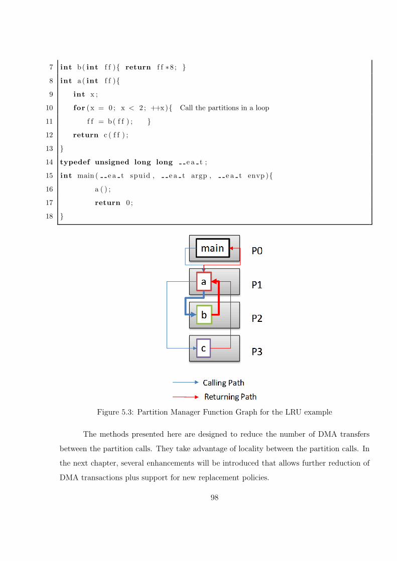
7 int b( int f f ){ return f f ∗8 ; }
8 int a ( int f f ){
9 int x ;
10 for ( x = 0 ; x < 2 ; ++x){ Call the partitions in a loop
11 f f = b( f f ) ; }
12 return c ( f f ) ;
13 }
14 typedef unsigned long long e a t ;
15 int main ( e a t spuid , e a t argp , e a t envp ){
16 a ( ) ;
17 return 0 ;
18 }
Figure 5.3: Partition Manager Function Graph for the LRU example
The methods presented here are designed to reduce the number of DMA transfers
between the partition calls. They take advantage of locality between the partition calls. In
the next chapter, several enhancements will be introduced that allows further reduction of
DMA transactions plus support for new replacement policies.
98
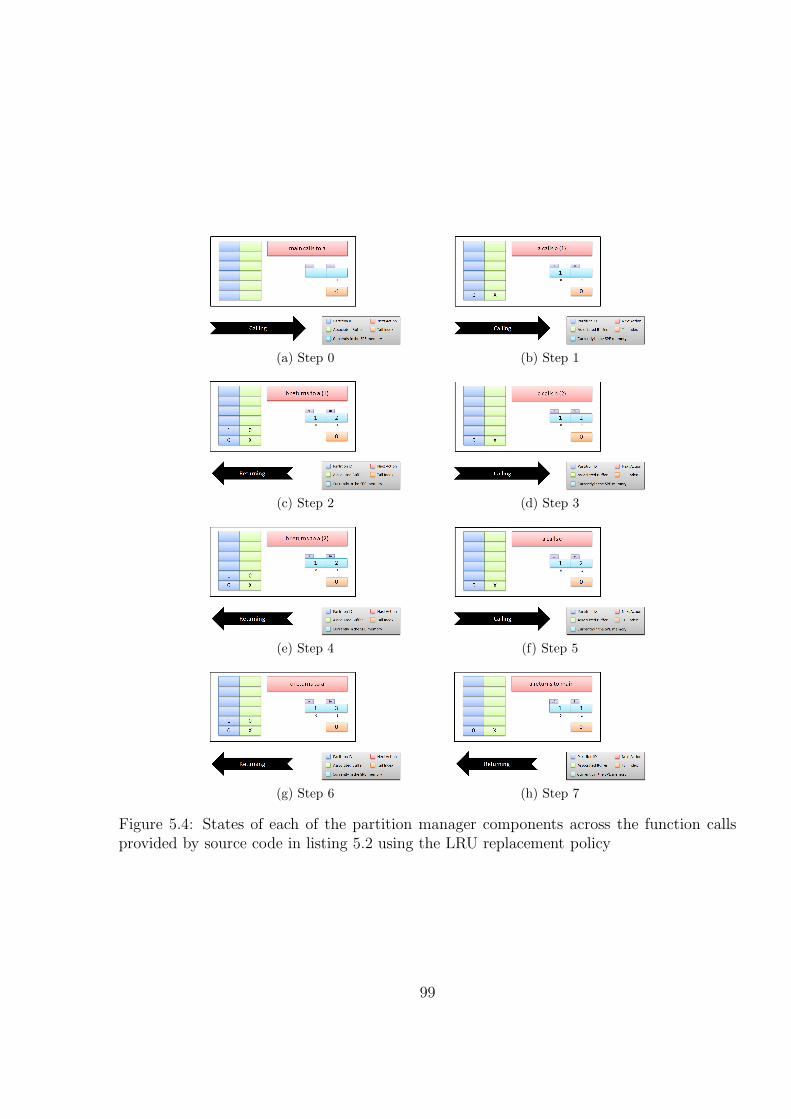
(a) Step 0 (b) Step 1
(c) Step 2 (d) Step 3
(e) Step 4 (f) Step 5
(g) Step 6 (h) Step 7
Figure 5.4: States of each of the partition manager components across the function callsprovided by source code in listing 5.2 using the LRU replacement policy
99
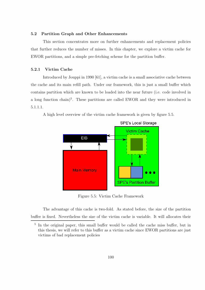
5.2 Partition Graph and Other Enhancements
This section concentrates more on further enhancements and replacement policies
that further reduces the number of misses. In this chapter, we explore a victim cache for
EWOR partitions, and a simple pre-fetching scheme for the partition buffer.
5.2.1 Victim Cache
Introduced by Jouppi in 1990 [61], a victim cache is a small associative cache between
the cache and its main refill path. Under our framework, this is just a small buffer which
contains partition which are known to be loaded into the near future (i.e. code involved in
a long function chain)5. These partitions are called EWOR and they were introduced in
5.1.1.1.
A high level overview of the victim cache framework is given by figure 5.5.
Figure 5.5: Victim Cache Framework
The advantage of this cache is two-fold. As stated before, the size of the partition
buffer is fixed. Nevertheless the size of the victim cache is variable. It will allocates their
5 In the original paper, this small buffer would be called the cache miss buffer, but inthis thesis, we will refer to this buffer as a victim cache since EWOR partitions are justvictims of bad replacement policies
100
entries dynamically and deallocate them according to use or need (e.g. if the application
runs out of memory).
Dynamic entries are added between the partition buffers and the global memories in
the SPE’s heap. An entry in this area will consists of the code, its partition and sub-buffer
ids and a counter which counts its uses. When an EWOR partition is evicted, the entries
are checked to see if the partition is already in the heap. If there is a previous instance
of the partition, its counter is incremented. If there is no instance of this partition, new
memory is allocated, the ids are updated and the code is copied over.
If the application uses the provided memory allocation wrappers (wmalloc and wfree),
they check if the heap has enough memory over to allocate to the application requested
data. If the dynamic allocation fails, the wmalloc function will tear down the victim cache
framework and try to allocate the application memory region again. If the wrapper are not
used, the application will just return that it cannot allocate the memory without tearing
down the victim cache.
There is a drawback to this technique though. There is a trade-off between the
number of victim cache entries and the partition stack length. Since we need to know which
partition are EWOR in the partition stack, the partition stack must be traversed. However,
this is solved by using a mask to set the bit that represents the partition identifying number.
This scheme can reduce the number of code misses and it will not increase the
memory usage unless it needs to. Another method to reduce the misses is explained next
and it involves a static structure called the partition graph.
5.2.2 Prefetching
Prefetching is a very common idea used in most systems today. Under these systems,
they use compiler analysis, dynamic learning or locality ideas to prefetch application’s data
(data in this instance being code or data).
Under OPELL, prefetching is useful on predicting the next function to be called dur-
ing a function chain. Although this has been analyzed statically (and part of our approach
uses a static structure)[81], the utilization of the partition buffer is dynamically assigned.
101
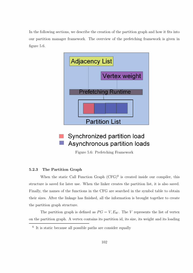
In the following sections, we describe the creation of the partition graph and how it fits into
our partition manager framework. The overview of the prefetching framework is given in
figure 5.6.
Figure 5.6: Prefetching Framework
5.2.3 The Partition Graph
When the static Call Function Graph (CFG)6 is created inside our compiler, this
structure is saved for later use. When the linker creates the partition list, it is also saved.
Finally, the names of the functions in the CFG are searched in the symbol table to obtain
their sizes. After the linkage has finished, all the information is brought together to create
the partition graph structure.
The partition graph is defined as PG = V,EW . The V represents the list of vertex
on the partition graph. A vertex contains its partition id, its size, its weight and its loading
6 It is static because all possible paths are consider equally
102
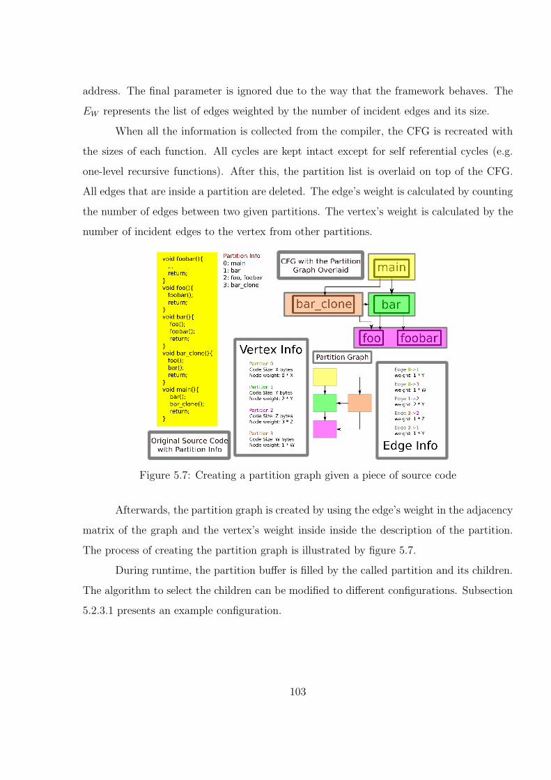
address. The final parameter is ignored due to the way that the framework behaves. The
EW represents the list of edges weighted by the number of incident edges and its size.
When all the information is collected from the compiler, the CFG is recreated with
the sizes of each function. All cycles are kept intact except for self referential cycles (e.g.
one-level recursive functions). After this, the partition list is overlaid on top of the CFG.
All edges that are inside a partition are deleted. The edge’s weight is calculated by counting
the number of edges between two given partitions. The vertex’s weight is calculated by the
number of incident edges to the vertex from other partitions.
Figure 5.7: Creating a partition graph given a piece of source code
Afterwards, the partition graph is created by using the edge’s weight in the adjacency
matrix of the graph and the vertex’s weight inside inside the description of the partition.
The process of creating the partition graph is illustrated by figure 5.7.
During runtime, the partition buffer is filled by the called partition and its children.
The algorithm to select the children can be modified to different configurations. Subsection
5.2.3.1 presents an example configuration.
103
5.2.3.1 Prefetching: Weighted Breadth First Fetch
When an partition load is activated (either by an initial load or a replacement), the
replacement policy is activated. Under the prefetching scheme, there exists two partition
types: the required partition and their children. When the required partition is loaded, the
framework will sort its children by its vertex weight times the edge weight (parent to child).
Next, the framework loads the N − 1 top children without interrupting the application.
In this case, N represents the number of sub-buffers that the partition buffer can be sub-
divided into. If the assumption is correct, then the child becomes the required partition and
its children will be loaded accordingly to the previous rules. If the required partition is not
in the buffer then the guess is wrong and the required partition must be loaded again. Since
the children partitions are loaded in a non-blocking fashion, they can overlap computation
and save time.
The sorting of the children is done before hand so it will not affect performance. The
two parameters (the vertex’s and edge’s weights) contains information about the usability
of the partition code and its relationship with its siblings. A higher number indicates that
they are more edges coming and going from the vertex and its child together with both code
sizes.
Although this technique does not reduce DMA traffic, it overlaps the computation
and communication more effectively and it can reduce misses by actively loading the children
into the sub-buffers.
All these techniques (the replacement policies and the victim caches) can be used
together to create a simple (yet effective) task management system.
5.2.4 Dynamic Code Enclaves
Dynamic Code Enclaves or DYCEs are a side effect of the usage of the partition
manager and its techniques. Thanks to its compiler support, the code created for the
partitions can be loaded anywhere in the running application and by using the ideas from
the victim cache feature, code regions can be created on the fly.
104
Since the partition manager deals with address and symbol resolutions, the branches
are intercepted by the framework and redirected to the correct tasks. This redirection is
achieved by passing the partition id to the caller (which might reside in another processor
altogether).
Finally, techniques like the lazy reuse and prefetching can be used to exploit the
inherent locality of the task.
In the next chapter, several overheads and experimental results are presented for all
techniques used for this framework.
105
Chapter 6
EXPERIMENTAL TESTBED AND RESULTS
The partition manager framework uses a small suite of test programs dedicated to
test its functionality and correctness. The testbed framework is called Harahel and it is
composed of several Perl scripts and test applications. The next subsections will explain
the hardware and software testbeds and presents results for each of the test programs.
6.1 Hardware Testbed
For these experiments, we use the Playstation 3’s CBE configuration. This means
a Cell processor with 6 functional SPE, 256 MiB of main memory, and 80 GiB of hard
drive space. The two disabled SPEs are used for redundancy and to support the hypervisor
functionality. Besides these changes, the CBE processor has the same facilities as high end
first generation CBE processors. We take advantage of the timing capabilities of the CBE
engine. The CBE engine has hardware time counters which ticks at a slower rate than the
main processor (in our case, they click at 79.8 MHz). Since they are hardware based, the
counters provided minimal interference with the main program. Each of the SPEs contains
a single counter register which can be accessed through our own timing facilities.
6.2 Software Testbed
For our experiments, we use a version of Linux running on the CBE, i.e. Yellow
Dog with a 2.6.16 kernel. Furthermore, we use the CBE toolchain version 1.1 but with an
upgraded GCC compiler, 4.2.0, which was ported to the CBE architecture for OpenOPELL
purposes.
The applications being tested include kernels used in many famous benchmarks.
This testbed includes the GZIP compression and decompression application which is our
106
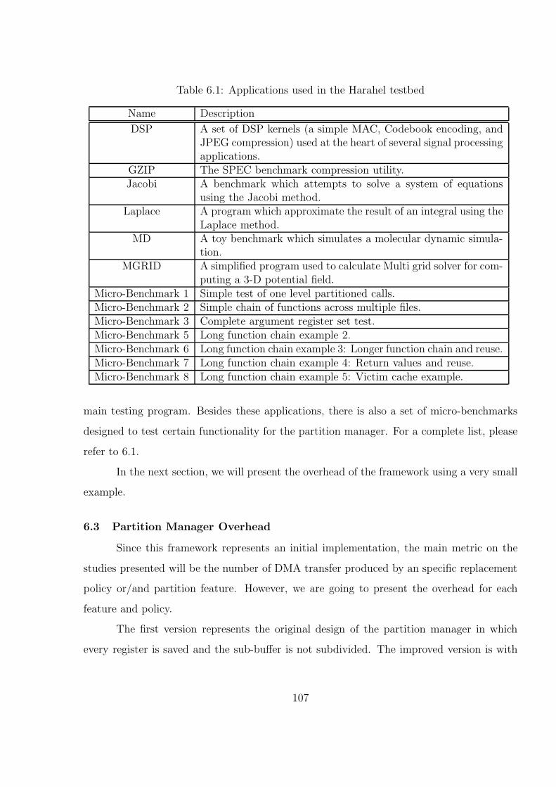
Table 6.1: Applications used in the Harahel testbed
Name Description
DSP A set of DSP kernels (a simple MAC, Codebook encoding, andJPEG compression) used at the heart of several signal processingapplications.
GZIP The SPEC benchmark compression utility.Jacobi A benchmark which attempts to solve a system of equations
using the Jacobi method.Laplace A program which approximate the result of an integral using the
Laplace method.MD A toy benchmark which simulates a molecular dynamic simula-
tion.MGRID A simplified program used to calculate Multi grid solver for com-
puting a 3-D potential field.Micro-Benchmark 1 Simple test of one level partitioned calls.Micro-Benchmark 2 Simple chain of functions across multiple files.Micro-Benchmark 3 Complete argument register set test.Micro-Benchmark 5 Long function chain example 2.Micro-Benchmark 6 Long function chain example 3: Longer function chain and reuse.Micro-Benchmark 7 Long function chain example 4: Return values and reuse.Micro-Benchmark 8 Long function chain example 5: Victim cache example.
main testing program. Besides these applications, there is also a set of micro-benchmarks
designed to test certain functionality for the partition manager. For a complete list, please
refer to 6.1.
In the next section, we will present the overhead of the framework using a very small
example.
6.3 Partition Manager Overhead
Since this framework represents an initial implementation, the main metric on the
studies presented will be the number of DMA transfer produced by an specific replacement
policy or/and partition feature. However, we are going to present the overhead for each
feature and policy.
The first version represents the original design of the partition manager in which
every register is saved and the sub-buffer is not subdivided. The improved version is with
107
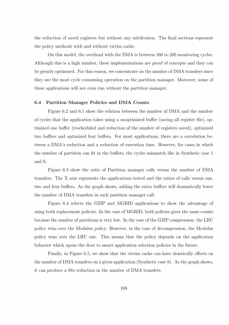
the reduction of saved registers but without any subdivision. The final sections represent
the policy methods with and without victim cache.
On this model, the overhead with the DMA is between 160 to 200 monitoring cycles.
Although this is a high number, these implementations are proof of concepts and they can
be greatly optimized. For this reason, we concentrate on the number of DMA transfers since
they are the most cycle consuming operation on the partition manager. Moreover, some of
these applications will not even run without the partition manager.
6.4 Partition Manager Policies and DMA Counts
Figure 6.2 and 6.1 show the relation between the number of DMA and the number
of cycles that the application takes using a unoptimized buffer (saving all register file), op-
timized one buffer (rescheduled and reduction of the number of registers saved), optimized
two buffers and optimized four buffers. For most applications, there are a correlation be-
tween a DMA’s reduction and a reduction of execution time. However, for cases in which
the number of partition can fit in the buffers, the cycles mismatch like in Synthetic case 1
and 6.
Figure 6.3 show the ratio of Partition manager calls versus the number of DMA
transfers. The X axis represents the applications tested and the ratios of calls versus one,
two and four buffers. As the graph shows, adding the extra buffers will dramatically lower
the number of DMA transfers in each partition manager call.
Figure 6.4 selects the GZIP and MGRID applications to show the advantage of
using both replacement policies. In the case of MGRID, both policies gives the same counts
because the number of partitions is very low. In the case of the GZIP compression, the LRU
policy wins over the Modulus policy. However, in the case of decompression, the Modulus
policy wins over the LRU one. This means that the policy depends on the application
behavior which opens the door to smart application selection policies in the future.
Finally, in Figure 6.5, we show that the victim cache can have drastically effects on
the number of DMA transfers on a given application (Synthetic case 8). As the graph shows,
it can produce a 88x reduction in the number of DMA transfers.
108

(a) DSP (b) GZIPC (c) GZIPD (d) JACOBI
(e) LAPLACE (f) MD (g) MGRID (h) SYNTH1
(i) SYNTH2 (j) SYNTH3 (k) SYNTH5 (l) SYNTH6
(m) SYNTH7 (n) SYNTH8
Figure 6.1: DMA counts for all applications for an unoptimized one buffer, an optimizedone buffer, optimized two buffers and optimized four buffer versions
109
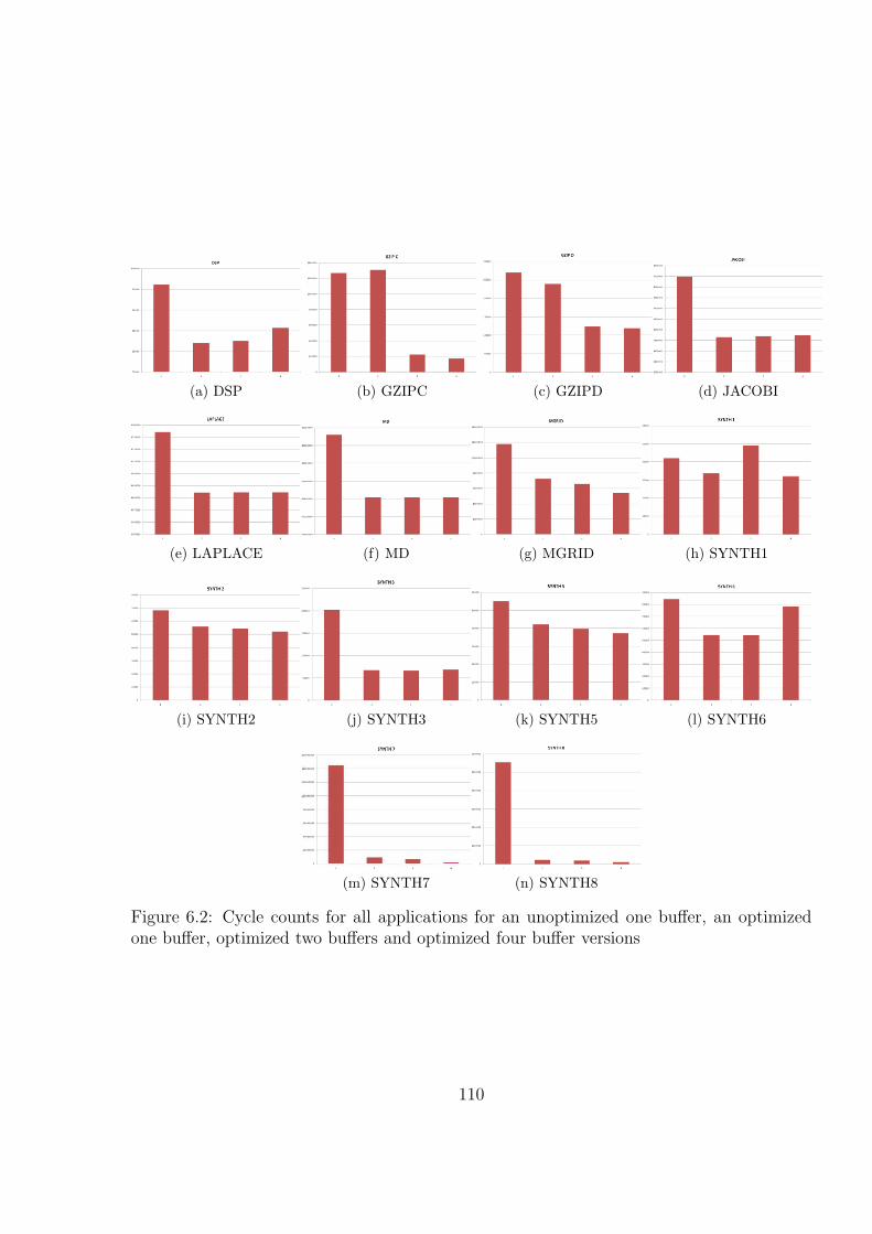
(a) DSP (b) GZIPC (c) GZIPD (d) JACOBI
(e) LAPLACE (f) MD (g) MGRID (h) SYNTH1
(i) SYNTH2 (j) SYNTH3 (k) SYNTH5 (l) SYNTH6
(m) SYNTH7 (n) SYNTH8
Figure 6.2: Cycle counts for all applications for an unoptimized one buffer, an optimizedone buffer, optimized two buffers and optimized four buffer versions
110
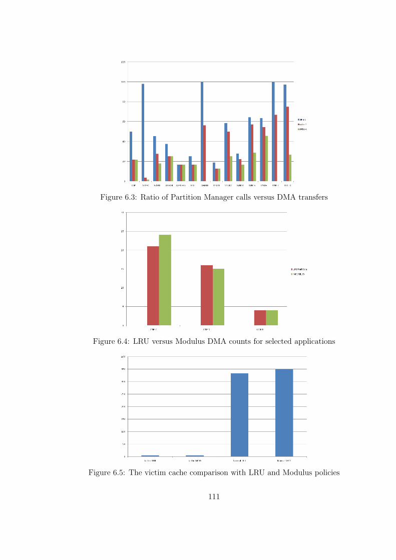
Figure 6.3: Ratio of Partition Manager calls versus DMA transfers
Figure 6.4: LRU versus Modulus DMA counts for selected applications
Figure 6.5: The victim cache comparison with LRU and Modulus policies
111
Chapter 7
RELATED WORK
The concept of overlays has been around for a long time. They were very useful in the
first multi-users systems and in systems which has restricted memory problems. However,
advances in hardware and software technologies have relegated them out of mainstream to
less visible areas of computing (i.e. embedded systems) [89]. There were two technologies
that displaced the overlay out of existence: dynamic libraries and virtual memory[32]. One
of the most famous early implementations of both concepts can be found in the Multiplexed
Information and Computing Service (MULTICS)[12][28].
7.1 A Historical Perspective
Before virtual memory, programs were manually separated into regions of code and
data. These regions were loaded as required. This was prevalent in systems during the 1940’s
and 1950’s in which the memory hierarchy was composed of at least two levels (permanent
storage and RAM). The first virtual memory prototype was proposed in [40] for the ATLAS
system. Under this system, the concept of address and memory location was decoupled and
the address translation units were born. Virtual memory automatically partitions the code
and data into predefined pages and loads them when needed. Structures like the Translation
Look-aside Buffer[36] were put into place to take advantage of the locality of code and data
pages. Thanks for virtual memory, programs could use much more than the available
physical memory and several of them can be run in the system as time shared fashion.
During the 1960s, the virtual memory concept spread like wildfire. Commercial systems like
the IBM 360/67[19], CDC 7600[43], Burroughs 6500[55] among others implemented virtual
memory. Of course, nowadays almost every general purpose system uses virtual memory[33].
112
Since then, there are several research efforts that concentrate on optimizing virtual memory
for multiple threads, like the one that uses smart pre-fetching on virtual pages based on
pattern of synchronized variables[63] and using different replacement policies[9].
Virtual memory has severe limitations for real time systems. It is not desirable for
performance sensitive applications. Moreover, programmers and users cannot even hint to
the virtual memory system about the location of their program nor influence the size of the
paging required per function or code region[33]1. Our partition approach allows the user
hints for the overlay creation and the runtime can modify the size of the code overlay buffers.
This can change per application and even per code region which makes my approach finer
grained.
Dynamic (shared) libraries are functions which are loaded on demand and are de-
signed to reduce the code image size. A way to implement these functions is to redirect
these calls to a special program (like the one pointed by the .inter segment under the ELF
program) which manages a dynamic function table. This table’s entries are function point-
ers that are populated by the special program. A function’s entry possesses a counter which
shows how many calls to this function call are in existence. When the counter reaches zero,
the entry can be reused. Consider that under this framework, the function code is not
moved around, they just reside in global memory and they are accessed by each required
process. The table is shared across many processes and threads that require these func-
tions. This saves memory footprint since the code is not replicated[93]2. As shown before,
these frameworks will not consider the locality of the code and they will not replicate to
local memory (to reduce latencies) since they posses instruction caches and virtual memory.
These systems are not designed for many core as the partition manager is since it loads
code according to its usage to their respective local (near) memory.
Finally, dynamic loading can load code on demand and unloaded it if necessary
during the application execution. This allows for dynamic optimization and bug fixing
1 Some Operating Systems and Computers allows to modify the page size but this appliesto every application on the system afterwards.
2 However, the data sections for each function are replicated for each user
113
without the need of restarting the whole system[93]. Moreover, it is commonly used to
implement software plug-ins for several service based programs like Web servers[41] and
Instant messenger programs. Finally, the IBM/360 Operating systems[4] line used these
feature for its I/O subroutines among others. As before, this system does not takes care
of locality and near memory issues because they were handled by the Virtual memory
subsystem. Under the partition manager framework, these issues are taking care by the
partition manager and it can decode the appropriate memory region to load the code.
7.1.1 The Embedded Field: Where Overlays Survived
As stated before, overlays and partitions survived in the embedded field. They usually
use classical overlays for code and other interesting techniques for data. Research presented
in [76] shows a dynamic approach for overlays for code. In this paper, a dynamic compiler
creates overlays according to the state of the memory. Moreover, it automatically creates
entry points for each application. However, this framework does not try to optimize the
access patterns using locality or learned patterns as the partition manager does. Moreover,
this is for low end embedded systems. However, there is no reason why these ideas could
not apply to the computational engines of future super computers.
Another research presented in [56] shows how the concept of overlaying plus dynamic
code compacting can increase performance by almost 50% for selected application (i.e.
SPLASH2[91]). It uses a clustering algorithm (at runtime) for basic blocks very similar to
the one in used in the partition manager compiler. However, they do not use any of the
locality opportunities for reuse like the partition manager does.
7.1.2 Data Movements in High Performance Computing
Finally, there is the concept of percolation introduced under the Hybrid Technology
Multi-Threaded (HTMT) Architecture[49]. The HTMT project proposed a highly config-
urable multiple levels (in computational components and memory levels). It was proposed
at the end 1990 decades and incorporated many state of the art concepts and technologies.
The concept of percolation was introduced to better utilize resources in such a machine.
It was introduced as the ability of migrate code and data regions to fast memory for each
114
component that needs it. It is called percolation because code / data regions trickle down
the hierarchy towards the processing elements. Please do not confuse this concept with the
percolation theory concept is mathematics that deal with the interconnectivity of connected
cluster in random graphs. An interesting research is conducted in [45], [46] and [44]. They
implement semi automatic data movement in explicit memory hierarchies for the Cyclops-
64. This technique is called “Tile Percolation” as it is the first of its kind to introduce the
concept of data locales under OpenMP. Both this technique and the partition manager can
be put together to implement a complete percolation engine if necessary.
7.2 Programmability for Cell B.E.
There have been many attempts to increase the programmability in the Cell B.E.
The most famous ones are the ALF and DaCS[14] frameworks and the CellSS project[10].
The ALF and DaCS frameworks are designed to facilitate the creation of tasks and data
communication respectively for the Cell B.E. The Accelerator Library Framework (ALF)
is designed to provide a user-level programming framework for people developing for the
Cell Architecture. It takes care of many low level approaches (like data transfers, task
management, data layout communication, etc). The DaCS framework provides support for
process management, accelerator topology services and several data movement schemas.
It is designed to provide a higher abstraction to the DMA engine communication. Both
frameworks can work together and they are definitely a step forward from the original Cell
B.E. primitives. They are not targeted to Cell B.E. application programmers, but to library
creators. Thus, the frameworks are designed to be lower level than expected for an OpenMP
programmer.
The Cell SuperScalar project (the CellSS) [10], and later the StarSS project[7], is
designed to automatically exploit the function parallelism of a sequential program and
distribute them across the Cell B.E. architecture. It accomplishes this with a set of pragma
based directives. It has a locality aware scheduler to better utilize the memory spaces. It
uses a very similar approach as OpenMP. However, it is restricted to task level parallelism
in comparison to OpenMP that can handle data level parallelism. Under our framework,
115
the parallel functions are analogous to CellSS tasks and the partition manager is their
scheduler. Many of the required attributes of the tasks under CellSS are hidden by the
OpenMP directives and pragmas which make them more programmable.
There have been efforts to port OpenMP to the Cell B.E.. The most successful one is
the implementation in IBM’s XL compiler[74]. The implementation under the XL compiler
is analogous to the OPELL implementation with very important differences. The software
cache under the XL compiler is not configurable with respect to the number of dirty bytes
that can be monitored in the line. This allows the implementation of novel memory models
and frameworks as shown in [17]. The other difference is that the partition manager under
the XL uses static GCC-like overlays. Under OPELL, the partitions can be dynamically
loaded anywhere in the memory which is not possible under the XL compiler.
Finally, there is a plethora of work that creates new frameworks to increase the
Cell B.E. productivity. Rapidmind introduced its high performance language that aims to
improve the productivity of the Cell B.E.[72]. It has data types designed to mask the data
movement and a framework that move data across the computational components according
to which function/data type is required. However, it does not have the functionality of more
mature languages like C and C++. Another effort is the porting of R-Stream to the Cell
B.E. [65] from Reservoir Labs. It provides several data movement functions to coordinate the
application’s behavior and performance. However, this approach is still low level compared
against an OpenMP implementation. Finally, we have graphical languages, like Gedae[66],
which aims to increase the usability of the Cell B.E. but at the cost of ignoring certain
optimization opportunities. Moreover, this project is closed and proprietary unlike OPELL.
7.3 Future Directions
Another research direction worth taking a look is into Instruction Cache coloring as
represented in [81] and [54]. These research concentrates on static analysis of certain code
templates (i.e. loops, control statements, etc) to maximize their reuse in the instruction
cache. They are very powerful techniques that uses weights according to the control struc-
ture involved, i.e. loops have weights equivalent to their number of iterations, the if/else
116
condition will represent 50% of the total weight for each path, and switch statements will
have 1 / number of cases per path. With these weights, function call graph is created and
a coloring algorithm is applied to prevent conflicts in the I-Cache.
7.4 Productivity Studies
Finally, we need to make a comparison between P3I and the Pittsburgh Productivity
study[15]. The study done in Pittsburgh was bigger and with more participants and pro-
gramming languages (UPC[13], X10[35] and Java). Although they have more man power,
they did not have the weight parameters, as P3I had, to represent expertise.
117
Chapter 8
CONCLUSIONS
Ideas presented in this paper show the trend of software in the many core age: the
software renaissance. Under this trend, old ideas are coming back to the plate: Overlays,
software caches, dataflow execution models, micro kernels, among others. This trend is
best shown in architectures like Cyclops-64[31] and the Cell B.E.’s SPE units. Both de-
signs exhibit explicit memory hierarchy, simple pipelines and the lack of virtual memory.
The software stacks on these architectures are in a heavily state of flux to better utilize
the hardware and increase productivity. This fertile research ground allows the reinvention
of these classic ideas. The partition manager frameworks rise from this flux. The simple
idea of having dynamic code regions is introduced in this thesis, in difference with regular
overlays, these partitions represent highly mobile code from which other framework can be
developed. In this thesis, the framework developed was to support OpenMP in a heteroge-
neous architecture. However, several research directions are still open, such as a stronger
static analysis, building on mature research such cache coloring for I-caches or dynamic
scheduling of code due to percolation constrains.
This thesis shows a framework to support the code movements across heterogeneous
accelerators components. It shows how these effort spans across all components of the
software stack. Moreover, it depicts its place on a higher abstraction framework for a
high level parallel programming language. It shows the effect of several policies dedicated
to reduce the number of high latency operations. This is just the start of the road for
many designs. The future is bright but it will require the rebirth and rethinking of many
components. That is why I called this a software renaissance in which classical concepts
will be used in novel ways and applied to million of cores that the future will bring.
118
BIBLIOGRAPHY
[1] Openmp: Simple, portable, scalable smp programming. http://www.openmp.org/
drupal. OpenMP Architecture Review Board.
[2] is openmp for users?, nov 2004. Invited presentation at OpenMP BOF, Supercomputing2004, Pittsburgh.
[3] Milena Milenkovic Aleksandar, Ar Milenkovic, and Jeffrey Kulick. Demystifying intelbranch predictors. In In Workshop on Duplicating, Deconstructing and Debunking,pages 52–61. John Wiley Sons, 2002.
[4] G. M. Amdahl, G. A. Blaauw, and F. P. Brooks, Jr. Readings in computer architec-ture. chapter Architecture of the IBM System/360, pages 17–31. Morgan KaufmannPublishers Inc., San Francisco, CA, USA, 2000.
[5] AnadTech. Amd’s 12-core magny-cours opteron 6174 vs. in-tel’s 6-core xeon. http://www.anandtech.com/show/2978/
amd-s-12-core-magny-cours-opteron-6174-vs-intel-s-6-core-xeon, mar2010.
[6] Arne Andersson and Stefan Nilsson. Implementing radixsort. J. Exp. Algorithmics, 3,September 1998.
[7] Eduard Ayguade, Rosa M. Badia, Francisco D. Igual, Jesus Labarta, Rafael Mayo, andEnrique S. Quintana-Ortı. An extension of the starss programming model for platformswith multiple gpus. In Proceedings of the 15th International Euro-Par Conference onParallel Processing, Euro-Par ’09, pages 851–862, Berlin, Heidelberg, 2009. Springer-Verlag.
[8] Paul S. Barth, Paul S. Barth, Arvind, Rishiyur S. Nikhil, and Rishiyur S. Nikhil.M-structures: Extending a parallel, non-strict, functional language with state, 1991.
[9] L. A. Belady. A study of replacement algorithms for a virtual-storage computer. IBMSyst. J., 5:78–101, June 1966.
[10] Pieter Bellens, Josep M. Perez, Rosa M. Badia, and Jesus Labarta. Cellss: a pro-gramming model for the cell be architecture. In ACM/IEEE CONFERENCE ONSUPERCOMPUTING, page 86. ACM, 2006.
119
[11] HPC Challenge benchmarks. The global updates per second benchmarks. the randomaccess program. http://icl.cs.utk.edu/projectsfiles/hpcc/RandomAccess/.
[12] A. Bensoussan, C.T. Clingen, and R. C. Daley. The multics virtual memory: Conceptsand design. Communications of the ACM, 15:308–318, 1972.
[13] Francois Cantonnet, Yiyi Yao, Mohamed M. Zahran, and Tarek A. El-Ghazawi. Pro-ductivity analysis of the upc language. In IPDPS. IEEE Computer Society, 2004.
[14] Jordi Caubet. Programming ibm powerxcell 8i / qs22 libspe2, alf, dacs. http:
//www.spscicomp.org/ScicomP15/slides/tutorial/programming-cell-ibm.pdf,may 2009.
[15] Pittsburgh Super Computing Center. Pittsburgh scientists measure productiv-ity in petascale supercomputing. http://www.psc.edu/publicinfo/news/2004/
2004-02-17_petascale.html, feb 2004.
[16] Daniel G. Chavarrıa-Miranda, Andres Marquez, Jarek Nieplocha, Kristyn J. Maschhoff,and Chad Scherrer. Early experience with out-of-core applications on the cray xmt. InIPDPS, pages 1–8, 2008.
[17] Chen Chen, Joseph B. Manzano, Ge Gan, Guang R. Gao, and Vivek Sarkar. A studyof a software cache implementation of the openmp memory model for multicore andmanycore architectures. In Euro-Par (2)’10, pages 341–352, 2010.
[18] Andrew A. Chien. Lecture 21: Global address space machines. Lecture Class: Uni-versity of California at San Diego, Course Title: Theory of High Speed ParallelComputation, apr 1996. www-csag.ucsd.edu/individual/achien/cs433/Lectures/Lecture21.ps.
[19] Webb T. Comfort. A computing system design for user service. In Proceedings of theNovember 30–December 1, 1965, fall joint computer conference, part I, AFIPS ’65 (Fall,part I), pages 619–626, New York, NY, USA, 1965. ACM.
[20] AMD Corp. Amd corporation website. http://www.amd.com.
[21] IBM Corp. Cbe architectural manual. http://www.capsl.udel.edu/~jmanzano/
Cell/docs/arch/CBEA_01_pub.pdf.
[22] Intel Corp. Intel corporation website. http://www.intel.com.
[23] Intel Corp. Intel’s tick tock model. http://www.intel.com/technology/tick-tock/index.htm.
[24] Tilera Corp. Tile64 processor product brief. http://www.tilera.com/sites/
default/files/productbriefs/PB010_TILE64_Processor_A_v4.pdf.
120
[25] Intel Corporation. Intel unveils new product plans for high performance comput-ing. http://www.intel.com/pressroom/archive/releases/2010/20100531comp.
htm, May 2010.
[26] Tilera Corporation. http://www.tilera.com/.
[27] NVIDIA Corporations. Nvidia tesla gpu power world’s fastest supercom-puter. http://pressroom.nvidia.com/easyir/customrel.do?easyirid=
A0D622CE9F579F09&version=live&prid=678988&releasejsp=release_157, Oc-tober 2010.
[28] Robert C. Daley and Jack B. Dennis. Virtual memory, processes, and sharing in multics.Commun. ACM, 11:306–312, May 1968.
[29] DARPA. High productivity computer systems. http://www.highproductivity.org/.
[30] Hans de Vries. Looking at intel’s prescott die, part 2. http://www.chip-architect.com/news/2003_04_20_Looking_at_Intels_Prescott_part2.html, April 2003.
[31] Juan del Cuvillo, Weirong Zhu, Ziang Hu, and Guang R. Gao. Tiny threads: Athread virtual machine for the cyclops64 cellular architecture. Parallel and DistributedProcessing Symposium, International, 15:265b, 2005.
[32] Peter J. Denning. Virtual memory. ACM Computing Surveys, 2:153–189, 1970.
[33] Peter J. Denning. Before memory was virtual. In In the Beginning: Personal Recollec-tions of Software Pioneers, page http://cne.gmu.edu/p, 1996.
[34] Stephanie Donovan, Gerrit Huizenga Ibm, Andrew J. Hutton, Andrew J. Hutton,C. Craig Ross, C. Craig Ross, Linux Symposium, Linux Symposium, Linux Sympo-sium, Martin K. Petersen, Wild Open Source, and Philip Schwan. Lustre: Building afile system for 1,000-node clusters, 2003.
[35] K. Ebcioglu, V. Saraswat, and V. Sarkar. X10: an experimental language for highproductivity programming of scalable systems. In Proceeding of the Second Workshopon Productivity and Performance in High End Computers, pages 45 – 51, February2005.
[36] Stephane Eranian and David Mosberger. Virtual memory in the ia-64 linux kernel.http://www.informit.com/articles/article.aspx?p=29961&seqNum=4.
[37] Stuart Faulk, Adam Porter, John Gustafson, Walter Tichy, Philip Johnson, andLawrence Votta. Measuring hpc productivity. International Journal of High Per-formance Computing Applications, 2004:459–473, 2004.
[38] John Feo, David Harper, Simon Kahan, and Petr Konecny. Eldorado. In Proceedingsof the 2nd conference on Computing frontiers, CF ’05, pages 28–34, New York, NY,USA, 2005. ACM.
121
[39] Agner Fog. The microarchitecture of Intel, AMD and VIA CPUs, 2009. Available athttp://www.agner.org/optimize/#manuals.
[40] John Fotheringham. Dynamic storage allocation in the atlas computer, including anautomatic use of a backing store. Commun. ACM, 4:435–436, October 1961.
[41] Apache Foundation. Apache http server version 2.2 documentation: Dynamic sharedobjects. http://httpd.apache.org/docs/2.2/dso.html.
[42] Free Software Foundation. The gnu compiler collection. http://gcc.gnu.org.
[43] SCD Supercomputer Gallery. Control data corporation (cdc) 7600: 19711983. http:
//www.cisl.ucar.edu/computers/gallery/cdc/7600.jsp.
[44] Ge Gan and Joseph Manzano. Tl-dae: Thread-level decoupled access/execution foropenmp on the cyclops-64 many-core processor. In LCPC, pages 80–94, 2009.
[45] Ge Gan, Xu Wang, Joseph Manzano, and Guang Gao. Tile percolation: An openmptile aware parallelization technique for the cyclops-64 multicore processor. In HenkSips, Dick Epema, and Hai-Xiang Lin, editors, Euro-Par 2009 Parallel Processing,volume 5704 of Lecture Notes in Computer Science, pages 839–850. Springer Berlin /Heidelberg, 2009.
[46] Ge Gan, Xu Wang, Joseph Manzano, and Guang R. Gao. Tile reduction: The firststep towards tile aware parallelization in openmp. In IWOMP, pages 140–153, 2009.
[47] Guang R Gao. Landing gnu-based openmp on cell: Progress report and perspectives.Keynote for STI Center of Competence for the Cell Broadband Engine Processor work-shop, July 2007.
[48] Guang R. Gao and Joseph B Manzano. Topic 1: Parallel architecture lingo and commonused terms. Lecture class: Principles of Parallel Architectures. University of Delaware,2009.
[49] Guang R. Gao, Kevin B. Theobald, Andres Marquez, and Thomas Sterling. The htmtprogram execution model. Technical report, In Workshop on Multithreaded Execution,Architecture and Compilation (in conjunction with HPCA-4), Las Vegas, 1997.
[50] D. Genossar and N. Shamir. Intel pentium m power estimation, budgeting, optimiza-tion, and validation. Technical report, Intel Corporation, May 2003.
[51] S. Gochman, A. Mendelson, A. Naveh, and E. Rotem. Introduction to intel core duoprocessor architecture. Intelligence/sigart Bulletin, 2006.
[52] William Gropp. Tutorial on mpi: The message-passing interface. http://www.mcs.
anl.gov/research/projects/mpi/tutorial/gropp/talk.html.
122
[53] L Gwennap. New algorithm improves branch prediction. Microprocessor Report, pages17–21, Mar 1995.
[54] Amir H. Hashemi, David R. Kaeli, and Brad Calder. Efficient procedure mapping usingcache line coloring. In IN PROCEEDINGS OF THE SIGPLAN’97 CONFERENCEON PROGRAMMING LANGUAGE DESIGN AND IMPLEMENTATION, pages 171–182, 1997.
[55] E.A. Hauck and B.A. Dent. Burroughs’ b6500 / b7500 stack mechanism. http://www.cs.berkeley.edu/~culler/courses/cs252-s05/papers/burroughs.pdf.
[56] Haifeng He, Saumya K. Debray, and Gregory R. Andrews. The revenge of the overlay:automatic compaction of os kernel code via on-demand code loading. In Proceedings ofthe 7th ACM & IEEE international conference on Embedded software, EMSOFT ’07,pages 75–83, New York, NY, USA, 2007. ACM.
[57] H. Peter Hofstee. Power efficient processor architecture and the cell processor, 2005.San Francisco, CA.
[58] NCSA illinois. Blue waters: Sustained petascale computing. http://www.ncsa.
illinois.edu/BlueWaters/.
[59] The Inquirer. Intel 80 core chip revealed in full detail. http://www.theinquirer.net/inquirer/news/1026032/intel-80-core-chip-revealed, February 2007.
[60] Yi Jiang. Design and implementation of tool-chain framework to support openmp singlesource compilation on cell platform, 2007. Master Thesis Submission.
[61] Norman P. Jouppi. Improving direct-mapped cache performance by the addition of asmall fully-associative cache and prefetch buffers. In ISCA, pages 364–373, 1990.
[62] Nathan Kirsch. An overview of intel’s teraflops research chip. http://www.
legitreviews.com/article/460/1/, February 2007.
[63] Sang kwon Lee, Hee chul Yun, Joonwon Lee, and Seungryoul Maeng. Adaptive prefetch-ing technique for shared virtual memory, 2001.
[64] H. Q. Le, W. J. Starke, J. S. Fields, F. P. O’Connell, D. Q. Nguyen, B. J. Ronchetti,W. M. Sauer, E. M. Schwarz, and M. T. Vaden. Ibm power6 microarchitecture. IBMJ. Res. Dev., 51:639–662, November 2007.
[65] Allen Leung, Benot Meister, Nicolas Vasilache, David Wohlford, and Richard Lethin.Automatic high level compilation to the cell/b.e. with the polyhedral approach. http://sti.cc.gatech.edu/Slides2008/Leung-080710.pdf. Presented at the GT STICell Workshop 10 July 2008.
123
[66] William I. Lundgren. Gedae: Automated multithreading and system requirements forinteroperability. http://sti.cc.gatech.edu/Slides2008/Lundgren-080711.pdf.Presented at the GT STI Cell Workshop 10 July 2008.
[67] Joseph B. Manzano, Ge Gan, Juergen Ribuztka, Sunil Shrestha, and Guang R Gao.Opell and pm: A case study on porting shared memory programming models to accel-erators architectures. In Submitted to LCPC 2011, Sept 2011.
[68] Joseph B. Manzano, Ziang Hu, Yi Jiang, Ge Gan, Hyo-Jung Song, and Jung-Gyu Park.Toward an automatic code layout methodology. In IWOMP, pages 157–160, 2007.
[69] Wolfram Mathworld. Gram-schmidt orthonormalization. http://mathworld.
wolfram.com/Gram-SchmidtOrthonormalization.html.
[70] C. May, E. Silha, R. Simpson, and H. Warren, editors. The PowerPC Architecture.Morgan Kuffman, 2nd edition, 1994.
[71] C. May, E. Silha, R. Simpson, and H. Warren, editors. The PowerPC Architecture.Morgan Kuffman, 2nd edition, 1994.
[72] Michael D. McCool and Bruce D’Amora. Programming using rapidmind on the cellbe. In Proceedings of the 2006 ACM/IEEE conference on Supercomputing, SC ’06, NewYork, NY, USA, 2006. ACM.
[73] David Mosberger. Memory consistency models, 1993.
[74] Kevin O’Brien, Kathryn O’Brien, Zehra Sura, Tong Chen, and Tao Zhang. Supportingopenmp on cell. Int. J. Parallel Program., 36:289–311, June 2008.
[75] OpenMP. OpenMP Specification: version 3.0, May 2008.
[76] Hae-woo Park, Kyoungjoo Oh, Soyoung Park, Myoung-min Sim, and Soonhoi Ha.Dynamic code overlay of sdf-modeled programs on low-end embedded systems. InProceedings of the conference on Design, automation and test in Europe: Proceedings,DATE ’06, pages 945–946, 3001 Leuven, Belgium, Belgium, 2006. European Designand Automation Association.
[77] David A. Patterson and John L. Hennessy. Computer Architecture: A QuantitativeApproach. Morgan Kaufmann, fourth edition, 2006. Chapter Two: Instruction LevelParallelism and Its Exploitation.
[78] PCPlus. Building the exascale computer. http://pcplus.techradar.com/node/3072.
[79] Michael J. Quinn. Parallel Programming in C with MPI and OpenMP. McGraw-HillEducation Group, 2003.
[80] Dave Sager, Desktop Platforms Group, and Intel Corp. The microarchitecture of thepentium 4 processor. Intel Technology Journal, 1:2001, 2001.
124
[81] A. Dain Samples and Paul N. Hilfinger. Code reorganization for instruction caches.Technical Report UCB/CSD-88-447, EECS Department, University of California,Berkeley, Oct 1988.
[82] Vivek Sarkar, Clay Williams, and Kemal Ebcioglu. Application development pro-ductivity challenges for high-end computing. HPCA Workshop on Productivity andPerformance in High-End Computing, feb 2004.
[83] B. Sinharoy, R. N. Kalla, J. M. Tendler, R. J. Eickemeyer, and J. B. Joyner. Power5system microarchitecture. IBM J. Res. Dev., 49:505–521, July 2005.
[84] Balaram Sinharoy. Power7 multi-core processor design. In Proceedings of the 42ndAnnual IEEE/ACM International Symposium on Microarchitecture, MICRO 42, pages1–1, New York, NY, USA, 2009. ACM.
[85] Eric Sprangle, Robert S. Chappell, Mitch Alsup, and Yale N. Patt. The agree predictor:a mechanism for reducing negative branch history interference. In Proceedings of the24th annual international symposium on Computer architecture, ISCA ’97, pages 284–291, New York, NY, USA, 1997. ACM.
[86] Sun. OpenSPARC T2 Core Microarchitecture Specification, a edition, December 2007.
[87] Technologizer. Intels new 48 core processor wontchange your life. http://technologizer.com/2009/12/02/
intels-new-48-core-processor-wont-change-your-life/, 2009.
[88] Jay Trodden and Don Anderson. HyperTransport. Addison Wesley, 2003.
[89] Andrew C. Vogan. Overlays in ms-dos. http://www.cs.cofc.edu/\~leclerc/340/
MSDOS-by-Andrew-Vogan-2002-Fall.ppt, dec 2002.
[90] David Wentzlaff, Patrick Griffin, Henry Hoffmann, Liewei Bao, Bruce Edwards, CarlRamey, Matthew Mattina, Chyi-Chang Miao, John F. Brown III, and Anant Agarwal.On-chip interconnection architecture of the tile processor. IEEE Micro, 27:15–31, 2007.
[91] Steven Cameron Woo, Moriyoshi Ohara, Evan Torrie, Jaswinder Pal Singh, and AnoopGupta. The splash-2 programs: characterization and methodological considerations.SIGARCH Comput. Archit. News, 23:24–36, May 1995.
[92] Tse-Yu Yeh and Yale N. Patt. Two-level adaptive training branch prediction. InProceedings of the 24th annual international symposium on Microarchitecture, MICRO24, pages 51–61, New York, NY, USA, 1991. ACM.
[93] YoLinux.com. Static, shared dynamic and loadable linux libraries. http://www.
yolinux.com/TUTORIALS/LibraryArchives-StaticAndDynamic.html.
125
[94] Y. Zhang, J.B. Manzano, and G. Gao. Atomic section: Concept and implementation. InMid-Atlantic Student Workshop on Programming Languages and Systems (MASPLAS),apr 2005.
[95] Yuan Zhang, Weirong Zhu, Fei Chen, Ziang Hu, and Guang R. Gao. Sequential con-sistency revisit: The sufficient condition and method to reason the consistency modelof a multiprocessor-on-a-chip architecture. Parallel and Distributed Computing andNetworks (PDCN 2005), February 2005.
126