CHAPTER 12

Competition between crop and weeds: A system approach

C.J.T. SPITTERS and J.P. VAN DEN BERGH

1. Introduction

Weeds reduce crop yield because they compete with the crop for nutrients, water and light. Weed control measures are focused directly or indirectly on improving the competitive ability of the crop with regard to the weeds. In this chapter weed problems will be considered from the angle of competition.

We are in favour of a system-analytical ap­proach. System analysis means that the system as a whole is analysed, the relations within it being quantified. The equations for these relations are combined to a (simulation) model. A system ap­proach is especially useful in obtaining an outline of the relations within the system, their structure and the relative importance of each one. A simulation model also opens the possibility of predicting the results of situations not tested. Applied to weed problems: a better understanding is obtained on how the various methods of weed control affect competition between crop and weed and their effect can be predicted.

Baeumer and de Wit (1968) developed a simple model to simulate competition between different species. Competition between a crop and its weeds and the effect of weed control is discussed with this model. A competition experiment with wheat and ryegrass (Lolium rigidum Gaud.) (Rerkasem 1978) serves as a case study.

W. Holzner and N. Numata ( eds.), Biology and ecology of weeds. © 1982, Dr W. Junk Publishers, The Hague. ISBN 90 6193 682 9.

2. Design of competition experiments

Three types of competition experiments will be discussed: additive experiments, replacement (sub­stitution) experiments and experiments designed to simulate competition in time.

2.1 Additive experiments

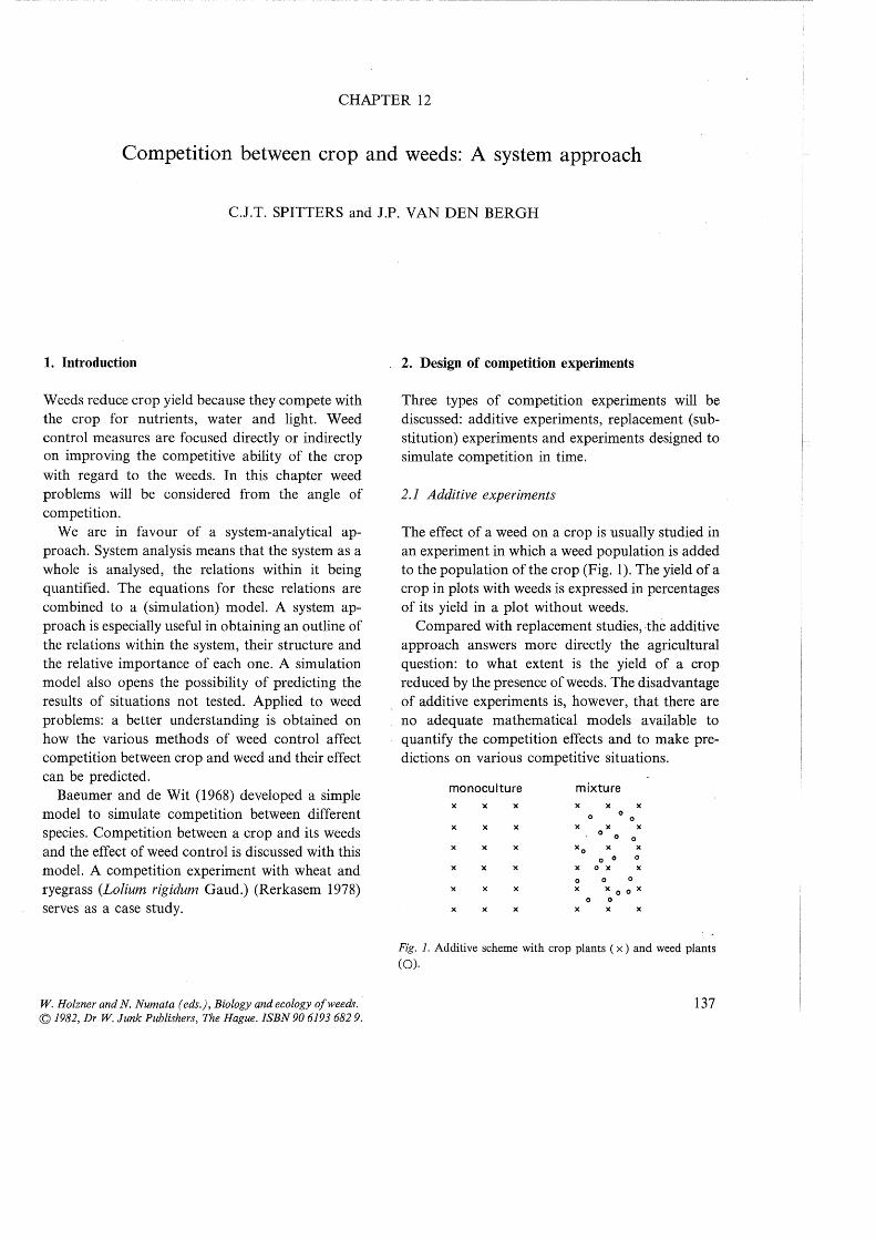
The effect of a weed on a crop is usually studied in an experiment in which a weed population is added to the population of the crop (Fig. 1 ). The yield of a crop in plots with weeds is expressed in percentages of its yield in a plot without weeds.

Compared with replacement studies, the additive approach answers more directly the agricultural question: to what extent is the yield of a crop reduced by the presence of weeds. The disadvantage of additive experiments is, however, that there are no adequate mathematical models available to quantify the competition effects and to make pre­dictions on various competitive situations.

monoculture mixture X X X X X X

0 0 0

X X X X X X 0

0 0 X X X xo X X

0 0 0

X X X X 0 X X

0 0 0

X X X X X 0 0 X

0 0

X X X X X X

Fig. I. Additive scheme with crop plants ( x ) and weed plants (0).

137

2.2 Replacement (substitution) experiments

In other fields of competition research the replace­ment principle is often used: a range of mixtures is generated by starting with a monoculture of species 1, progressively replacing plants of species 1 with those of species 2 until a monoculture of species 2 is obtained. As a result all stands have the same density (Fig. 2). Many models have been developed to quantify the competition effects in replacement experiments. De Wit's (1960) competition model has been shown to be the most adequate for this purpose (Trenbath 1978; Spitters 1979, pp. 27-36).

monocu ltu re mixture monoculture

of crop of weed )( )( )( )( 0 )( 0 0 0

)( )( )( 0 )( 0 0 0 0

)( )( )( X 0 X 0 0 0

)( X )( 0 X 0 0 0 0

)( )( X )( 0 X 0 0 0

X )( X 0 )( 0 0 0 0

Fig. 2. Replacement scheme with crop plants ( x ) and weed plants (o)

The drawback of replacement experiments is that they do not directly coincide with practical weed problems. Given the competitive relations at one density the yields of different mixtures at the same density can be predicted, but those at other densities only to a certain extent. So likewise with the additive schemes the possibility of generalizing the findings of one experiment with one method of weed control to other methods of control, is only limited. These drawbacks are avoided with dynamic simulation of the competition effects in time.

2.3 Dynamic simulation of competition

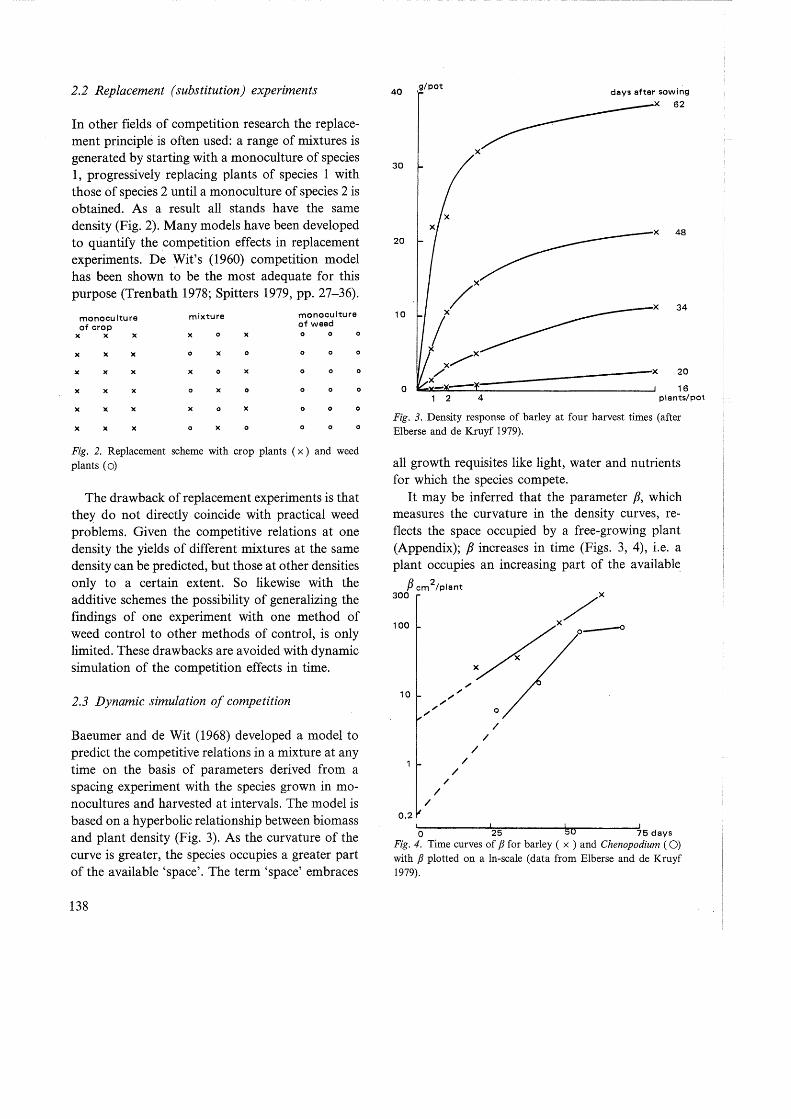
Baeumer and de Wit (1968) developed a model to predict the competitive relations in a mixture at any time on the basis of parameters derived from a spacing experiment with the species grown in mo­nocultures and harvested at intervals. The model is based on a hyperbolic relationship between biomass and plant density (Fig. 3). As the curvature of the curve is greater, the species occupies a greater part of the available 'space'. The term 'space' embraces

138

40 ,9/pot days after sowing

X 62

X

30

20

X 34 10

0 v----------------------x 20 16

1 2 4 plants/pot

Fig. 3. Density response of barley at four harvest times (after Elberse and de Kruyf 1979).

all growth requisites like light, water and nutrients for which the species compete.

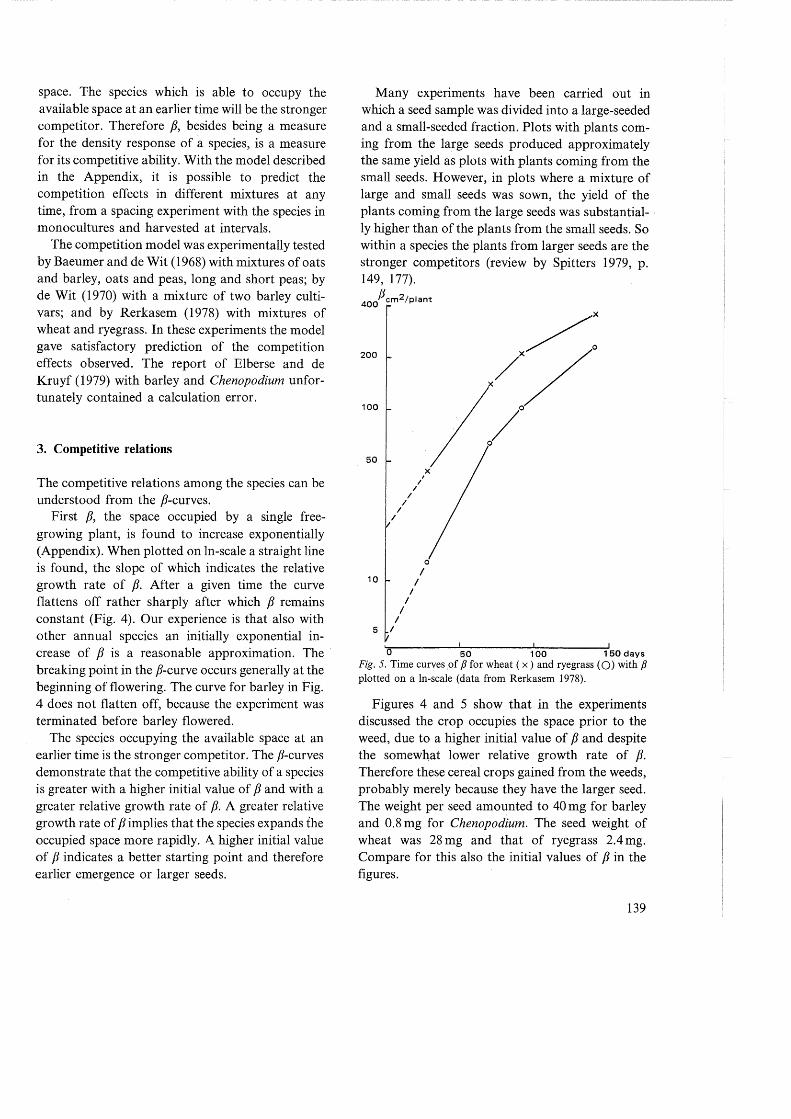
It may be inferred that the parameter p, which measures the curvature in the density curves, re­flects the space occupied by a free-growing plant (Appendix); P increases in time (Figs. 3, 4), i.e. a plant occupies an increasing part of the available

P cm2

/plant 300

100

10

0.2

/

/ /

/ /

0

/ /

/

I I I

0 25 ou 75 days

Fig. 4. Time curves of P for barley ( x ) and Chenopodium ( 0) with P plotted on a In-scale (data from Elberse and de Kruyf 1979).

space. The species which is able to occupy the available space at an earlier time will be the stronger competitor. Therefore /3, besides being a measure for the density response of a species, is a measure for its competitive ability. With the model described in the Appendix, it is possible to predict the competition effects in different mixtures at any time, from a spacing experiment with the species in monocultures and harvested at intervals.

The competition model was experimentally tested by Baeumer and de Wit (1968) with mixtures of oats and barley, oats and peas, long and short peas; by de Wit (1970) with a mixture of two barley culti­vars; and by Rerkasem (1978) with mixtures of wheat and ryegrass. In these experiments the model gave satisfactory prediction of the competition effects observed. The report of Elberse and de Kruyf (1979) with barley and Chenopodium unfor­tunately contained a calculation error.

3. Competitive relations

The competitive relations among the species can be understood from the /3-curves.

First /3, the space occupied by a single free­growing plant, is found to increase exponentially (Appendix). When plotted on In-scale a straight line is found, the slope of which indicates the relative growth rate of fJ. After a given time the curve flattens off rather sharply after which f3 remains constant (Fig. 4). Our experience is that also with other annual species an initially exponential in­crease of f3 is a reasonable approximation. The breaking point in the /3-curve occurs generally at the beginning of flowering. The curve for barley in Fig. 4 does not flatten off, because the experiment was terminated before barley flowered.

The species occupying the available space at an earlier time is the stronger competitor. The fJ-curves demonstrate that the competitive ability of a species is greater with a higher initial value of f3 and with a greater relative growth rate of fJ. A greater relative growth rate of f3 implies that the species expands ihe occupied space more rapidly. A higher initial value of f3 indicates a better starting point and therefore earlier emergence or larger seeds.

Many experiments have been carried out in which a seed sample was divided into a large-seeded and a small-seeded fraction. Plots with plants com­ing from the large seeds produced approximately the same yield as plots with plants coming from the small seeds. However, in plots where a mixture of large and small seeds was sown, the yield of the plants coming from the large seeds was substantial- · ly higher than of the plants from the small seeds. So within a species the plants from larger seeds are the stronger competitors (review by Spitters 1979, p. 149, 177).

400/J cm2/plant

200

100

50

10 1

I 5 I

I

I I

0

I

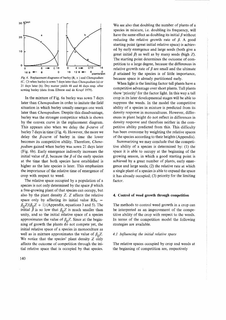
0 50 1 00 1 50 days Fig. 5. Time curves .of fJ for wheat ( x ) and rye grass ( 0) with fJ plotted on a In-scale (data from Rerkasem 1978).

Figures 4 and 5 show that in the experiments discussed the crop occupies the space prior to the weed, due to a higher initial value of f3 and despite the somewh,at lower relative growth rate of fJ. Therefore these cereal crops gained from the weeds, probably merely because they have the larger seed. The weight per seed amounted to 40mg for barley and 0.8 mg for Chenopodium. The seed weight of wheat was 28 mg and that of rye grass 2.4 mg. Compare for this also the initial values of f3 in the figures.

139

30r· I X:--......_ a

20 "" X

X

10

0 8 __. C 16 0 4--. C10 16

16 B -+- 8 0 16 12 B .,_. 6plal1tS/~ot

Fig. 6. Replacement diagrams of barley (B, x ) and Chenopodium (C, 0) when barley is sown 7 days later than Chenopodium (a) or 21 days later (b). Dry matter yields 48 and 46 days resp. after sowing barley (data from Elberse and de Kruyf 1979).

In the mixture of Fig. 6a barley was sown 7 days later than Chenopodium in order to imitate the field situation in which barley usually emerges one week later than Chenopodium. Despite this disadvantage, barley was the stronger competitor which is shown by the convex curve in the replacement diagram. This appears also when we delay the /]-curve of barley 7 days in time (Fig. 4). However, the more we delay the /]-curve of barley in time the lower becomes its competitive ability. Therefore, Cheno­podium gained when barley was sown 21 days later (Fig. 6b ). Early emergence indirectly increases the initial value of [J, because the fJ of the early species at the time that both species have established is higher as the late species is later. This emphasizes the importance of the relative time of emergence of crop with respect to weed.

The relative space occupied by a population of a species is not only determined by the space fJ which a free-growing plant of that species can occupy, but also by the plant density Z. Z affects the relative space only by affecting its initial value RS0 =

[J0Zf([JQZ + 1) (Appendix, equations 3 and 5). The initial jJ is so low that p0z is much smaller than unity, and so the initial relative space of a species approximates the value of p0z. Since at the begin­ning of growth the plants do not compete yet, the initial relative space of a species in monoculture as well as in mixture approximates the value of p

0z.

We notice that the species' plant density Z only affects the outcome of competition through the ini­tial relative space that is occupied by that species.

140

We see also that doubling the number of plants of a species in mixture, i.e. doubling its frequency, will have the same effect as doubling its initial fJ without reducing the relative growth rate of [J. A good starting point (great initial relative space) is achiev­ed by early emergence and large seeds (both give a great initial [J) as well as by many seeds (high Z). The starting point determines the outcome of com­petition to a large degree, because the differences in relative growth rate of fJ are small and the ultimate fJ attained by the species is of little importance, because space is already partitioned early.

When light is the limiting factor tall plants have a competitive advantage over short plants. Tall plants show 'priority' for the factor light. In this way a tall crop in its later developmental stages will be able to suppress the weeds. In the model the competitive ability of a species in mixture is predicted from its density response in monocultures. However, differ­ences in plant height do not reflect in differences in density response and therefore neither in the com­petitive ability predicted from this. This difficulty has been overcome by weighting the relative spaces of the species according to their heights (Appendix).

Summarizing we may conclude that the competi­tive ability of a species is determined by: ( 1) the space it is able to occupy at the beginning of the growing season, in which a good starting point is achieved by a great number of plants, early emer­gence and large seeds; (2) the relative rate at which a single plant of a species is able to expand the space it has already occupied; (3) priority for the limiting factor.

4. Control of weed growth through competition

The methods to control weed growth in a crop can be interpreted as an improvement of the compe­titive ability of the crop with respect to the weeds. In terms of the competition model the following strategies are available.

4.1 Influencing the initial relative space

The relative spaces occupied by crop and weeds at the beginning of competition are, respectively

yield as 0 /o weed-free control

100

50

0

0 500

300 plants/hi2

1 50 plants/hi 2

75 plants/hi2

ryegrass 2 plants/m

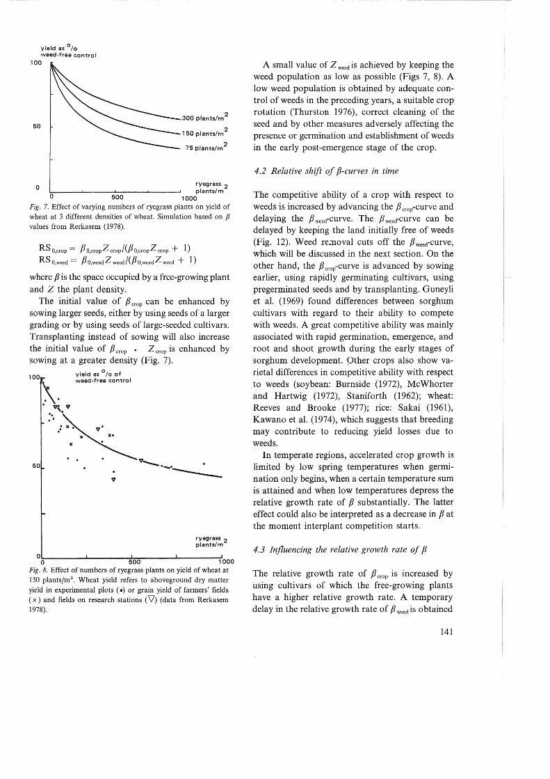
1000 Fig. 7. Effect of varying numbers of ryegrass plants on yield of wheat at 3 different densities of wheat. Simulation based on fJ values from Rerkasem (1978).

RS O,crop = f3 O,cropZ crop/(/3 o,cropZ crop + 1) RS o,weed = f3 o,weedZ weed/(/3 O,weedZ weed + 1)

where f3 is the space occupied by a free-growing plant and Z the plant density.

The initial value of f3 crop can be enhanced by sowing larger seeds, eitl~_er by using seeds of a larger grading or by using seeds of large-seeded cultivars. Transplanting instead of sowing will also increase the initial value of f3 crop • z crop is enhanced by sowing at a greater density (Fig. 7).

yield as 0 /o of weed-free control

ryegrass 2 plants/m

00~--------~------~5~0~0------~-------7

Fig. 8. Effect of numbers of ryegrass plants on yield of wheat at 150 plantsjm2

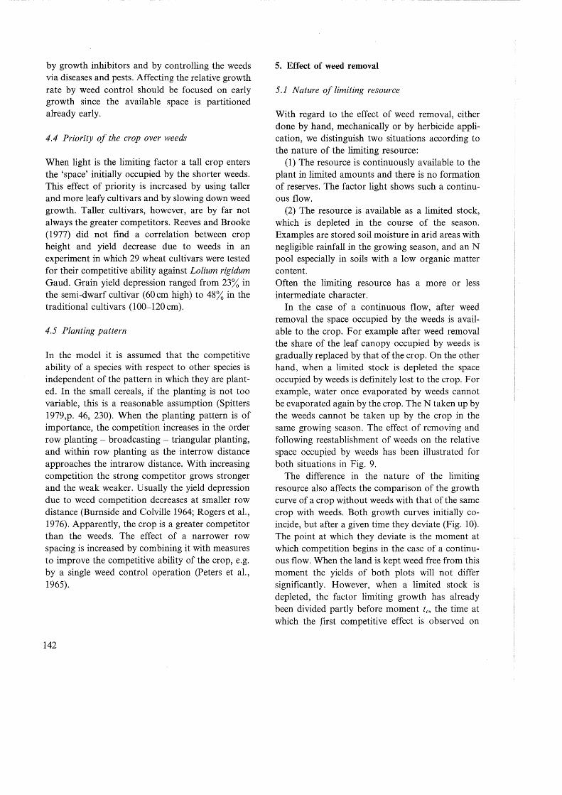
. Wheat yield refers to aboveground dry matter yield in experimental plots ( •) or grain yield of farmers' fields ( x) and fields on research stations (\!') (data from Rerkasem 1978).

A small value of Z weed is achieved by keeping the weed population as low as possible (Figs 7, 8). A low weed population is obtained by adequate con­trol of weeds in the preceding years, a suitable crop rotation (Thurston 1976), correct cleaning of the seed and by other measures adversely affecting the presence or germination and establishment of weeds in the early post-emergence stage of the crop.

4.2 Relative shift of f3-curves in time

The competitive ability of a crop with respect to weeds is increased by advancing the f3 crop-curve and delaying the f3 weed-curve. The f3 weecrcurve can be delayed by keeping the land initially free of weeds (Fig. 12). Weed re:noval cuts off the f3weed-curve, which will be discussed in the next section. On the other hand, the f3 crop-curve is advanced by sowing earlier, using rapidly germinating cultivars, using pregerminated seeds and by transplanting. Guneyli et al. (1969) found differences between sorghum cultivars with regard to their ability to compete with weeds. A great competitive ability was mainly associated with rapid germination, emergence, and root and shoot growth during the early stages of sorghum development. Other crops also show va­rietal differences in competitive ability with respect to weeds (soybean: Burnside (1972), McWhorter and Hartwig (1972), Staniforth (1962); wheat: Reeves and Brooke (1977); rice: Sakai (1961), Kawano et al. (1974), which suggests that breeding may contribute to reducing yield losses due to weeds.

In temperate regions, accelerated crop growth is limited by low spring temperatures when germi­nation only begins, when a certain temperature sum is attained and when low temperatures depress the relative growth rate of f3 substantially. The latter effect could also be interpreted as a decrease in f3 at the moment interplant competition starts.

4.3 Influencing the relative growth rate of f3

The relative growth rate of f3 crop is increased by using cultivars of which the free-growing plants have a higher relative growth rate. A temporary delay in the relative growth rate of f3weedis obtained

141

by growth inhibitors and by controlling the weeds via diseases and pests. Affecting the relative growth rate by weed control should be focused on early growth since the available space is partitioned already early.

4.4 Priority of the crop over weeds

When light is the limiting factor a tall crop enters the 'space' initially occupied by the shorter weeds. This effect of priority is increased by using taller and more leafy cultivars and by slowing down weed growth. Taller cultivars, however, are by far not always the greater competitors. Reeves and Brooke (1977) did not find a correlation between crop height and yield decrease due to weeds in an experiment in which 29 wheat cultivars were tested for their competitive ability against Lolium rigidum Gaud. Grain yield depression ranged from 23% in the semi-dwarf cultivar (60cm high) to 48% in the traditional cultivars (100-120cm).

4.5 Planting pattern

In the model it is assumed that the competitive ability of a species with respect to other species is independent of the pattern in which they are plant­ed. In the small cereals, if the planting is not too variable, this is a reasonable assumption (Spitters 1979 ,p. 46, 230). When the planting pattern is of importance, the competition increases in the order row planting - broadcasting - triangular planting, and within row planting as the interrow distance approaches the intrarow distance. With increasing competition the strong competitor grows stronger and the weak weaker. Usually the yield depression due to weed competition decreases at smaller row distance (Burnside and Colville 1964; Rogers et al., 1976). Apparently, the crop is a greater competitor than the weeds. The effect of a narrower row spacing is increased by combining it with measures to improve the competitive ability of the crop, e.g. by a single weed control operation (Peters et al., 1965).

142

5. Effect of weed removal

5.1 Nature -of limiting resource

With regard to the effect of weed removal, either done by hand, mechanically or by herbicide appli­cation, we distinguish two situations according to the nature of the limiting resource:

(1) The resource is continuously available to the plant in limited amounts and there is no formation of reserves. The factor light shows such a continu­ous flow.

(2) The resource is available as a limited stock, which is depleted in the course of the season. Examples are stored soil moisture in arid areas with negligible rainfall in the growing season, and an N pool especially in soils with a low organic matter content. Often the limiting resource has a more or less intermediate character.

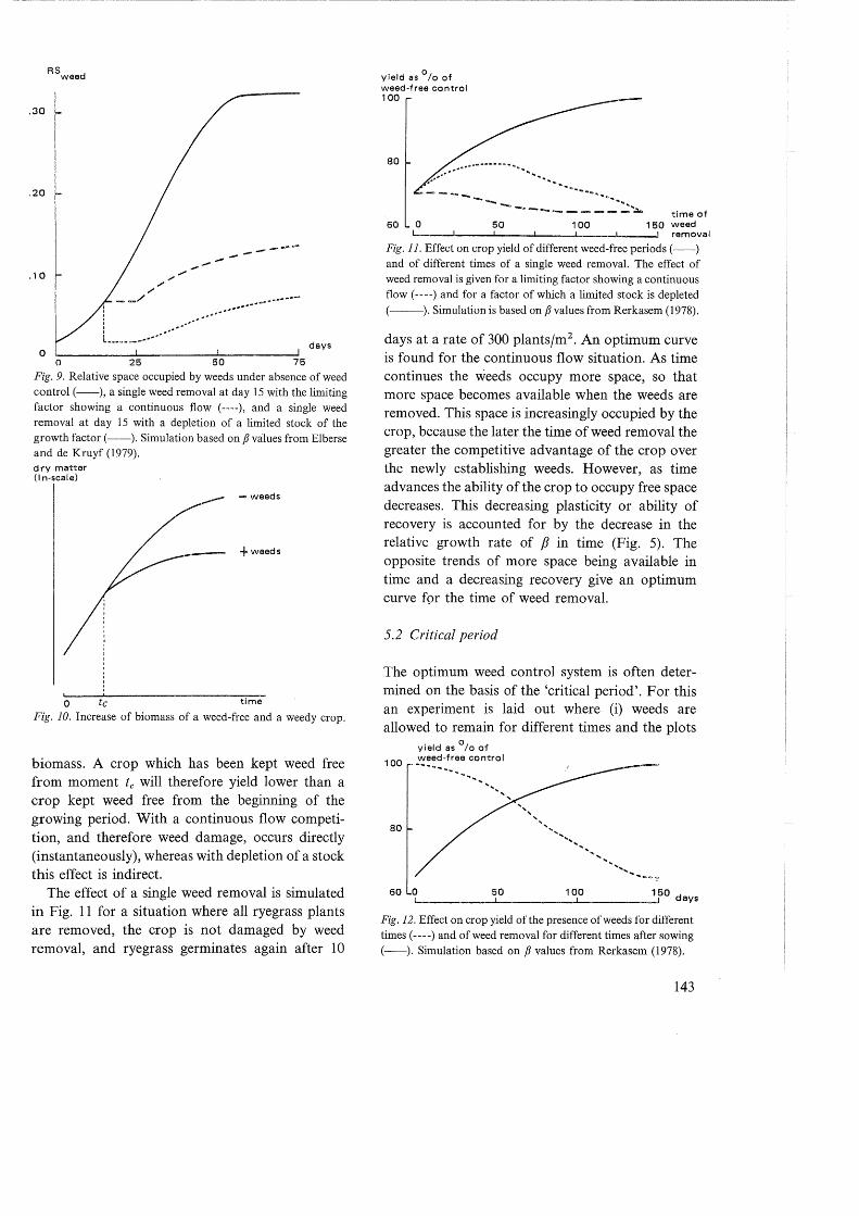
In the case of a continuous flow, after weed removal the space occupied by the weeds is avail­able to the crop. For example after weed removal the share of the leaf canopy occupied by weeds is gradually replaced by that of the crop. On the other hand, when a limited stock is depleted the space occupied by weeds is definitely lost to the crop. For example, water once evaporated by weeds cannot be evaporated again by the crop. The N taken up by the weeds cannot be taken up by the crop in the same growing season. The effect of removing and following reestablishment of weeds on the relative space occupied by weeds has been illustrated for both situations in Fig. 9.

The difference in the nature of the limiting resource also affects the comparison of the growth curve of a crop without weeds with that of the same crop with weeds. Both growth curves initially co­incide, but after a given time they deviate (Fig. 10). The point at which they deviate is the moment at which competition begins in the case of a continu­ous flow. When the land is kept weed free from this moment the yields of both plots will not differ significantly. However, when a limited stock is depleted, the factor limiting growth has already been divided partly before moment tc, the time at which the first competitive effect is observed on

.30

. 20

.10

0 0

... ····----····· ..... ·

...

-- ---

............ ...... .--·••co.,•

25 50 75

days

Fig. 9. Relative space occupied by weeds under absence of weed control (--), a single weed removal at day 15 with the limiting factor showing a continuous flow ( ----), and a single weed removal at day 15 with a depletion of a limited stock of the growth factor(--). Simulation based on p values from Elberse and de Kruyf (1979). dry matter (In-scale)

-weeds

+weeds

0 tc time

Fig. 10. Increase of biomass of a weed-free and a weedy crop.

biomass. A crop which has been kept weed free from moment tc will therefore yield lower than a crop kept weed free from the beginning of the growing period. With a continuous flow competi­tion, and therefore weed damage, occurs directly (instantaneously), whereas with depletion of a stock this effect is indirect.

The effect of a single weed removal is simulated in Fig. 11 for a situation where all ryegrass plants are removed, the crop is not damaged by weed removal, and rye grass germinates again after 10

yield as 0

/o of weed-free control 100

80 ··········-····~.q ............. ~ .... ~ .. ~ ..

------~~~~: .. ::".:,.. 60 0 50 100

time of 150 weed

removal

Fig. 11. Effect on crop yield of different weed-free periods(--) and of different times of a single weed removal. The effect of weed removal is given for a limiting factor showing a continuous flow(----) and for a factor of which a limited stock is depleted (--).Simulation is based on p values from Rerkasem (1978) .

days at a rate of 300 plantsfm2• An optimum curve

is found for the continuous flow situation. As time continues the weeds occupy more space, so that more space becomes available when the weeds are removed. This space is increasingly occupied by the crop, because the later the time of weed removal the greater the competitive advantage of the crop over the newly establishing weeds. However, as time advances the ability of the crop to occupy free space decreases. This decreasing plasticity or ability of recovery is accounted for by the decrease in the relative growth rate of f3 in time (Fig. 5). The opposite trends of more space being available in time and a decreasing recovery give an optimum curve for the time of weed removal.

5.2 Critical period

The optimum weed control system is often deter­mined on the basis of the 'critical period'. For this an experiment is laid out where (i) weeds are allowed to remain for different times and the plots

yield as 0 /o of weed-free control -............. ..., 100

80

so o~-.-_____ s.L.o _____ 1_o..~..o ____ -J150 days

Fig. 12. Effect on crop yield of the presence of weeds for ditTerent times(----) and of weed removal for different times after sowing (--). Simulation based on P values from Rerkasem (1978).

143

are then kept clean, and (ii) plots are kept clean for different initial periods and subsequent weeds are allowed to establish (Fig. 12). For example, Nieto et al. (1968) found that with maize and beans in Mexico, the critical period ran from 10 to 30 days after crop emergence, i.e. weeds present up to 10 days after crop emergence and those which appear­ed from 30 days onwards did not affect the yield. If weeds were left for longer than 10 days after emergence or weeding ceased before 30 days, the yield was reduced. When there is no critical period, a single weed operation at an appropriate time should be sufficient.

The curve in Fig. 12 reflecting the effect of the period that weeds were allowed to compete with the crop has been calculated for a limiting resource becoming available as a continuous flow. If, on the contrary, a limited stock were depleted the yield loss of the crop would be greater (Fig. 11) and so the criteria! period longer. This effect of the nature of the limiting resource might explain, why some authors found that already a short period of pre­sence of weeds after crop emergence reduced crop yield, whereas others with the same crop and the same weed species observed that yield reduction only occurred after a considerably longer period of presence of weeds.

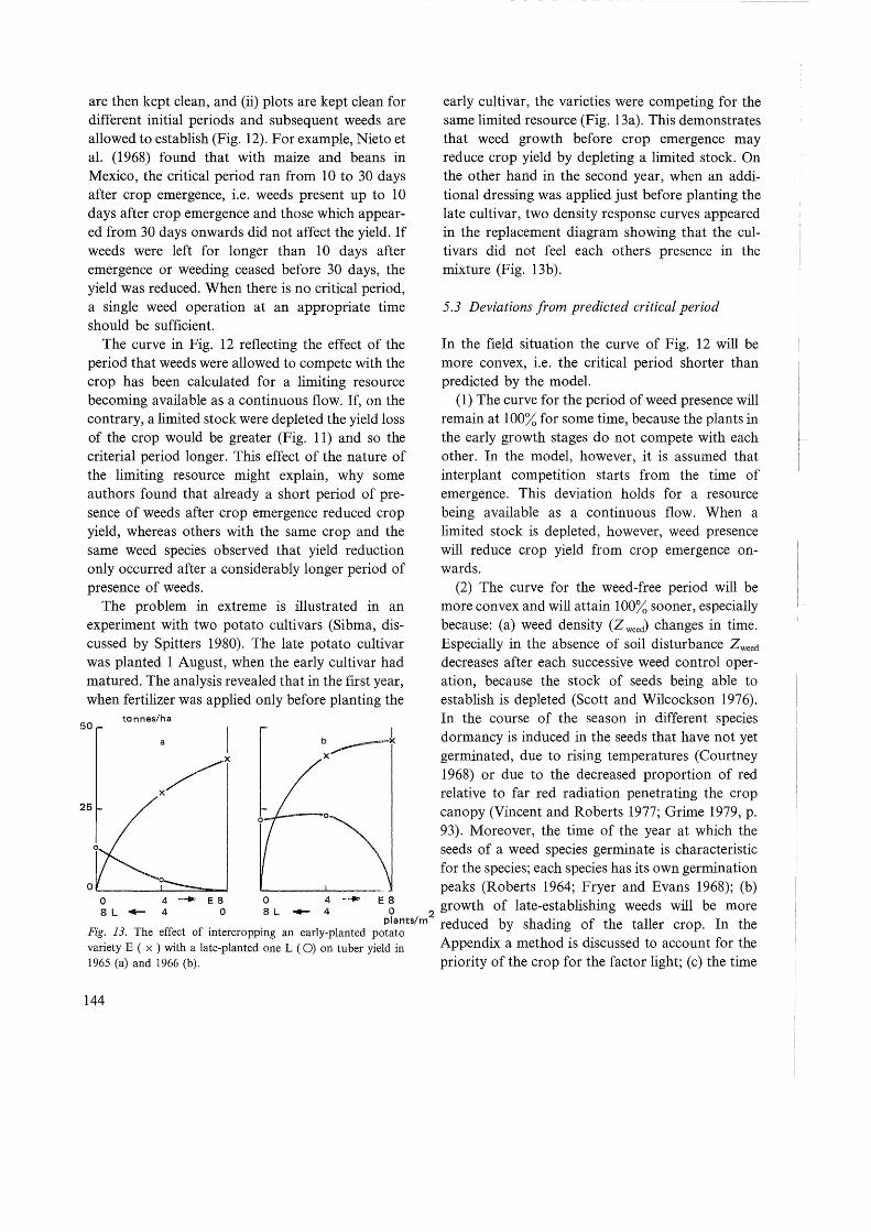
The problem in extreme is illustrated in an experiment with two potato cultivars (Sibma, dis­cussed by Spitters 1980). The late potato cultivar was planted 1 August, when the early cultivar had matured. The analysis revealed that in the first year, when fertilizer was applied only before planting the

50 tonnes/ha

I b~X X

early cultivar, the varieties were competing for the same limited resource (Fig. 13a). This demonstrates that weed growth before crop emergence may reduce crop yield by depleting a limited stock. On the other hand in the second year, when an addi­tional dressing was applied just before planting the late cultivar, two density response curves appeared in the replacement diagram showing that the cul­tivars did not feel each others presence in the mixture (Fig. 13b ).

5.3 Deviations from predicted critical period

In the field situation the curve of Fig. 12 will be more convex, i.e. the critical period shorter than predicted by the model.

(1) The curve for the period of weed presence will remain at 100% for some time, because the plants in the early growth stages do not compete with each other. In the model, however, it is assumed that interplant competition starts from the time of emergence. This deviation holds for a resource being available as a continuous flow. When a limited stock is depleted, however, weed presence will reduce crop yield from crop emergence on­wards.

(2) The curve for the weed-free period will be more convex and will attain 100% sooner, especially because: (a) weed density (Z weed> changes in time. Especially in the absence of soil disturbance Zweed decreases after each successive weed control oper­ation, because the stock of seeds being able to establish is depleted (Scott and Wilcockson 1976). In the course of the season in different species dormancy is induced in the seeds that have not yet germinated, due to rising temperatures (Courtney 1968) or due to the decreased proportion of red relative to far red radiation penetrating the crop canopy (Vincent and Roberts 1977; Grime 1979, p. 93). Moreover, the time of the year at which the seeds of a weed species germinate is characteristic for the species; each species has its own germination peaks (Roberts 1964; Fryer and Evans 1968); (b)

~ L ..,_ : -+ E ~ ~ L ~ 1 .._., E ~ 2

growth of late-establishing weeds will be more L''

13 Th r~ t f . t .

1 1 d plants/m reduced by shading of the taller crop. In the

rzg. . e e 1ec o m ercroppmg an ear y-p ante potato . . . variety E ( x ) with a late-planted one L ( 0) on tuber yield in Appendix a method IS dtscussed to account for the 1965 (a) and 1966 (b). priority of the crop for the factor light; (c) the time

144

1.5

a.-­---.b AYT = 1.5 1.2 1.0 1.0 1.0 0.8

>­a:

(I)

> ·;:; <0

"& 0 '·:~ r~ :tlJ: rn d.l%J

'------y-----1 partly indifferent and partly competitive exclusion comPetitive (niche differentiation) (exactly the same niche)

"hampering" effects

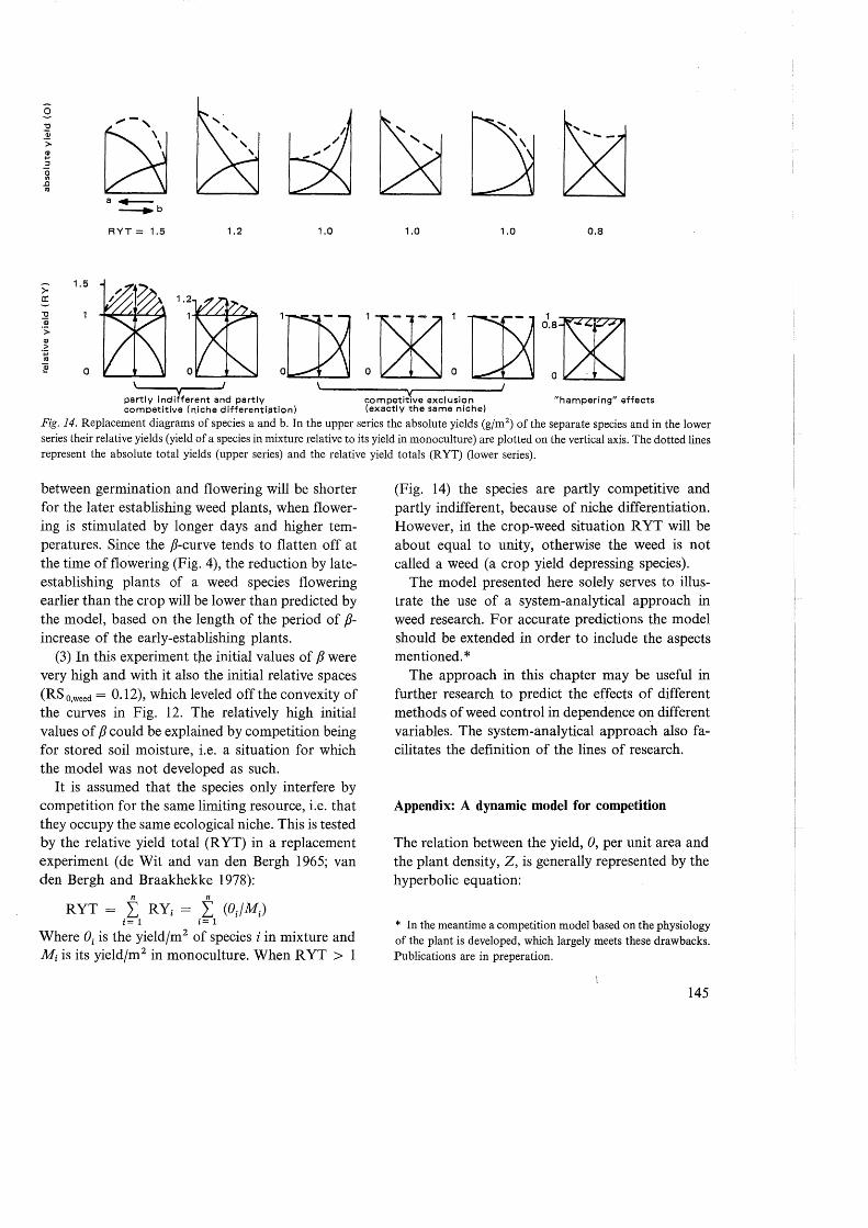
Fig. 14. Replacement diagrams of species a and b. In the upper series the absolute yields (gfm2 ) of the separate species and in the lower series their relative yields (yield of a species in mixture relative to its yield in monoculture) are plotted on the vertical axis. The dotted lines represent the absolute total yields (upper series) and the relative yield totals (RYT) (lower series).

between germination and flowering will be shorter for the later establishing weed plants, when flower­ing is stimulated by longer days and higher tem­peratures. Since the fJ-curve tends to flatten off at the time of flowering (Fig. 4), the reduction by late­establishing plants of a weed species flowering earlier than the crop will be lower than predicted by the model, based on the length of the period of fJ­increase of the early-establishing plants.

(3) In this experiment t}le initial values of fJ were very high and with it also the initial relative spaces (RS o,weed = 0.12), which leveled off the convexity of the curves in Fig. 12. The relatively high initial values of fJ could be explained by competition being for stored soil moisture, i.e. a situation for which the model was not developed as such.

It is assumed that the species only interfere by competition for the same limiting resource, i.e. that they occupy the same ecological niche. This is tested by the relative yield total (R YT) in a replacement experiment (de Wit and van den Bergh 1965; van den Bergh and Braakhekke 1978):

n n

RYT = I RYi = I (OJM) i= 1 i= 1

Where Oi is the yieldjm2 of species i in mixture and Mi is its yieldjm 2 in monoculture. When R YT > 1

(Fig. 14) the species are partly competitive and partly indifferent, because of niche differ~ntiation. However, in the crop-weed situation RYT will be about equal to unity~ otherwise the weed is not called a weed (a crop yield depressing species).

The model presented here solely serves to illus­trate the use of a system-analytical approach in weed research. For accurate predictions the model should be extended in order to include the aspects mentioned.*

The approach in this chapter may be useful in further research to predict the effects of different methods of weed control in dependence on different variables. The system-analytical approach also fa­cilitates the definition of the lines of research.

Appendix: A dynamic model for competition

The relation between the yield, 0, per unit area and the plant density, Z, is generally represented by the hyperbolic equation:

* In the meantime a competition model based on the physiology of the plant is developed, which largely meets these drawbacks. Publications are in preperation.

145

100

50

0

• /3 1/Z

Fig. 15. Relation between yield per unit area (0) and plant density (Z).

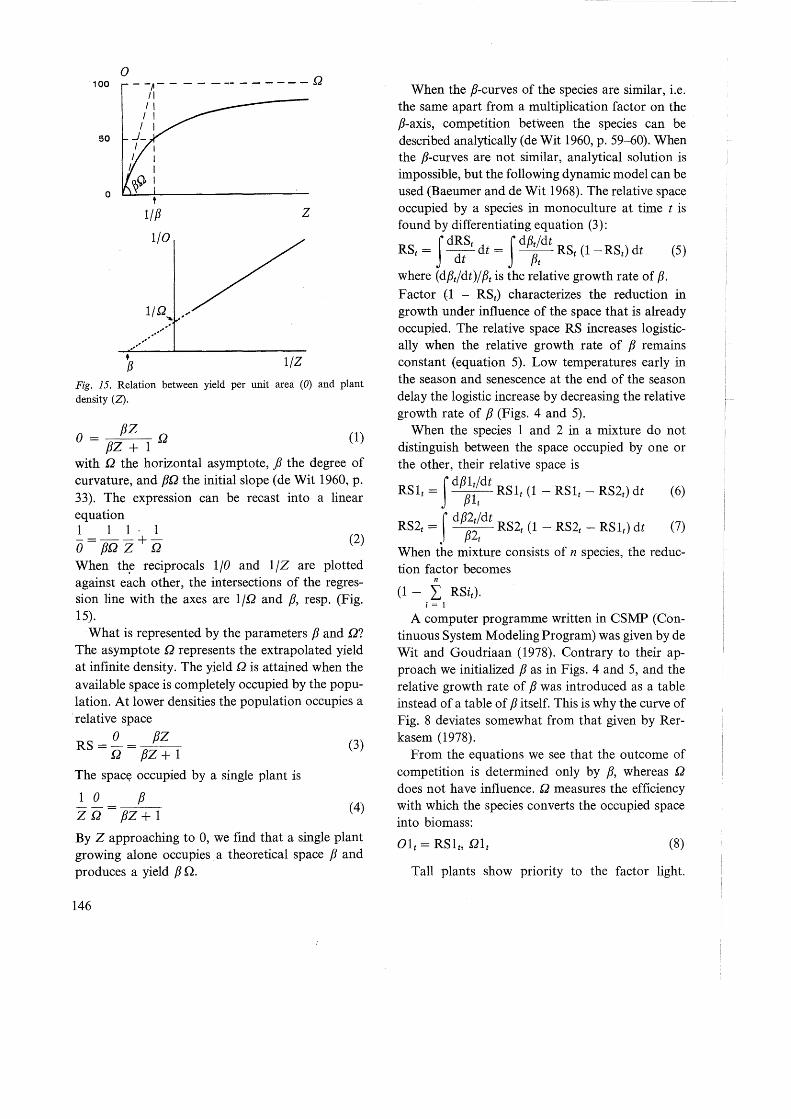
o = pz 1 a (1) pz +

with Q the horizontal asymptote, j3 the degree of curvature, and pa the initial slope (de Wit 1960, p. 33). The expression can be recast into a linear equation 1 1 1 . 1 o= paz+ Q C2)

When th~ reciprocals lJO and 1/Z are plotted against each other, the intersections of the regres­sion line with the axes are ljQ and p, resp. (Fig. 15).

What is represented by the parameters p and Q?

The asymptote Q represents the extrapolated yield at infinite density. The yield Q is attained when the available space is completely occupied by the popu­lation. At lower densities the population occupies a ·relative space

o pz RS = Q = pz + 1 (3)

The spac(( occupied by a single plant is

1 0 p z a pz + 1

(4)

By Z approaching to 0, we find that a single plant growing alone occupies . a theoretical space P and produces a yield p n.

146

When the P-curves of the species are similar, i.e. the same apart from a multiplication factor on the P-axis, competition between the species can be described analytically (de Wit 1960, p. 59--60). When the P-curves are not similar, analytical solution is hnpossible, but the following dynamic model can be used (Baeumer and de Wit 1968). The relative space occupied by a species in monoculture at time t is found by differentiating equation (3):

J dRSt J df3tfdt

RSt = dtdt = ~RSt (1-RSt) dt (5)

where (dptfdt)/f3t is the relative growth rate of f3. Factor (1 - RSt) characterizes the reduction in growth under influence of the space that is already occupied. The relative space RS increases logistic­ally when the relative growth rate of P remains constant (equation 5). Low temperatures early in the season and senescence at the end of the season delay the logistic increase by decreasing the relative growth rate of p (Figs. 4 and 5).

When the species 1 and 2 in a mixture do not distinguish between the space occupied by one or the other, their relative space is

J df31tfdt

RS1t = f31t RS1t (1 - RS1t - RS2t) dt (6)

1 df32tfdt RS2t = I f32t RS2t (1 - RS2t - RS1t) dt (7)

When the mixture consists of n species, the reduc-tion factor becomes

n

(1- L RSit). i = 1

A computer programme written in CSMP (Con­tinuous System Modeling Program) was given by de Wit and Goudriaan (1978). Contrary to their ap­proach we initialized pas in Figs. 4 and 5, and the relative growth rate of p was introduced as a table instead of a table of P itself. This is why the curve of Fig. 8 deviates somewhat from that given by Rer­kasem (1978).

From the equations we see that the outcome of competition is determined only by p, whereas Q

does not have influence. Q measures the efficiency with which the species converts the occupied space into biomass:

(8)

Tall plants show priority to the factor light.

However, differences in plant height are not re­flected in differences in p, which magnitude is estimated from the density response in monocul­tures. Baeumer and de Wit (1968) obviated this by weighting in the reduction factor the relative spaces of the species according to their heights, H:

J d,B1t/dt H2t

RSlt = ,Blt RSlt (1- RSlt- Hlt RS2t)dt (9)

Although de Wit did not explicitly mention it, it is assumed in the model that the resource for which the species compete is continuously available to the plant in limited amounts. Only competition for a factor demonstrating such a continuous flow affects biomass directly. However, Fig. 8 demonstrates that when a limited stock is depleted, in this case stored soil moisture in western Australia, the model may also give a satisfactory fit. Competition for a limited stock is simulated better by applying the equations to the amount of the limiting resource taken up instead of the biomass. When N is the limiting resource, RS is then the amount of N taken up divided by the total amount ofN being available for the plants.

It is assumed that the plants compete with each other from the time of emergence. However, in their initial growth in the field the species do not feel each others presence. In that case the relation between biomass and density is not exactly hyperbolic, but in: -the early growth stages and at low densities linear. Therefore, the curve reflecting the period of weed competition after crop emergence (Fig. 12) will remain for some time at 100% before curving down. Taking this into account, the species in the mixture of the model would have to be grown as in a monoculture until the time that interplant com­petition begins. In an experiment with two barley cultivars on nutrient solution in a climate room with light as the limiting resource it was demon­strated that exponential growth terminated and inter-cultivar competition started at the time when ground area covered was about 95% (Zonneveld and Spitters, unpubl.).

Estimating p and Q. Parameter p measures the degree of curvature of the density response curve. In the early growth stages this curve is almost linear (Fig. 3), and therefore the estimates of ,8 and Q will be unreliable. In the later growing stages only the

yields at very wide spacings are not yet in the horizontal part of the curve, which emphasizes the use of very divergent densities. The reliability of ,B's

and D's estimated for different harvest times may therefore differ considerably. The estimates may be improved by smoothing the curves of the calculated Q's. Q, the yield of a closed green crop canopy, increases approximately linearly in time (de Wit 1970). Based on the smoothed Q's, fJ is recal­culated.

References

Baeumer, K. and C.T. de Wit (1968). Competitive interference of plant species in monoculture and mixed stands. Neth. J. agric. Sci. 16: 103-122.

Bergh, J.P. van den and W.G. Braakhekke (1978). Coexistence of plant species by niche differentiation. In: Structure and functioning of plant populations. A.H.J. Freysen and J.W. Woldendorp (eds). Versl. Kon. Ned. Akad. Wet., Afd. Na­tuurk. 2e reeks, 70: 125-138. North-Holland Publ. Co., Amsterdam.

Burnside, O.C. (1972). Tolerance of soybean cultivars to weed competition and herbicides. Weed Sci. 20: 294-297.

Burnside, O.C. and W.L. Colville (1964). Soybean and weed yields as affected by irrigation, row spacing, tillage, and amiben. Weeds 12: 109-112.

Courtney, A.D. (1968). Seed dormancy and field emergence in Polygonum aviculare. J. appl. Ecol. 6: 675-684.

Elberse, W.T. and H.N. de Kruyf (1979). Competition between Hordeum vulgare L. and Chenopodium album L. with different dates of emergence of Chenopodium album. Neth. J. agric. Sci. 27: 13-26.

Fryer, J.D. and S.A. Evans (1968). The biology of weeds. In: Weed Control Handbook 5th ed. Blackwell Sci. Publ. 1: 1-24. Oxford. Grime, J.P. (1979). Plant strategies and vegetation processes.

John Wiley & Sons, Chichestor, New York, Brisbane, To­ronto, 222 pp.

Guneyli, E., O.C. Burnside andP.T. Nordquist (1969). Influence of seedling characteristics on weed competitive ability of sorghum hybrids and inbred lines. Crop Sci. 9: 713-716.

Kawano, K., H. Gonzalez and M. Lucena (1974). Intraspecific competition, competition with weeds, and spacing response in rice. Crop Sci. 14: 841-845.

McWhorter, C.G. and E.E. Hartwig (1972). Competition of johnsongrass and cocklebur with six soybean varieties. Weed Sci. 20: 56-59.

Nieto, H.J., M.A. Brondo and J.T. Gonzalez (1968). Critical periods of the crop growth cycle for competition from weeds. Pest Articles and News Summaries C14: 159-166.

147

Peters, E.J., M.R. Gebhardt and J.P. Stritzke (1965). Inter­relations of row spacings, cultivations and herbicides for weed control in soybeans. Weeds 13: 285-289.

Reeves, T.G. and H.D. Brooke (1977). The effect of genotype and phenotype on the competition between wheat and annual ryegrass. Proc. 6th Asian-Pacific Weed Sci. Conf. Jakarta, 166-171.

Rerkasem, K. (1978). Associated growth of wheat and annual ryegrass and the effect on yield and yield components of wheat. PhD Thesis, Dept Agron., Univ. Western Australia, 212 + 182 pp.

Roberts, H.A. (1964): Emergence and longevity in cultivated soils of seeds of some· annual weeds. Weed Res. 4: 296-307.

Roger.s, N.K., G.A. Buchanan and W.C. Johnson (1976). Influence of row spacing on weed competition with cotton. Weed Sci. 24: 410-413.

Sakai, K.I. (1961). Competitive ability in plants: its inheritance and some related problems. Symp. Soc. exp. Bioi. 15:245-263.

Scott, R.K. and S.J. Wilcockson (1976). Weed biology and the growth of sugar beet. Am1. appl. Bioi. 83: 331-335.

Spitters, C.J.T. (1980). Competition effects within mixed stands. In: Opportunities for increasing crop yields, R.G. Hurd, P.V. bouwk. Onderz.) 893, Pudoc, Wageningen, 268 pp.

148

Splitters, C.J.T. (1980). Competition effects within mixed stands. In: Opportunities for increasing crop yields, R.G. Hurd, P.V. Biscoe and C. Dennis (eds), Pitman Publ. Ltd. (in press).

Staniforth, D.W. (1962). Responses of soybean varieties to weed competition. Agron. J. 54: 11-13.

Thurston, J.M. (1976). Weeds in cereals in relation to agricul­tural practices. Ann. appl. Bioi. 83: 338-341.

Trenbath, B.R. (1978). Models and the interpretation of mixture experiments. In: Plant relations in pastures, J.R. Wilson (ed.), pp. 145-162. CSIRO, Melbourne.

Vincent, E.M. and E.H. Roberts (1977). The interaction oflight, nitrate and alternating temperature in promoting the germi­nation of dormant seeds of common weed species. Seed Sci. and Technol. 5: 569-670.

Wit, C.T. de (1960). On competition. Versl.landbouwk. Onderz. (Agric. Res. Rep.) 66 (8), Pudoc, Wageningen, 82 pp.

Wit, C.T. de (1970). On the modelling of competitive pheno­mena. Proc. Adv. Study Inst. Dynamics Numbers Popul. pp. 269-281. Oosterbeek, Netherlands.

Wit, C.T. de and J.P. vah den Bergh (1965). Competition between herbage plants. Neth. J. agric. Sci. 13: 212-221.

Wit, C.T. de and J. Goudriaan (1978). Simulation of ecological processes, 2nd ed. Pudoc, Wageningen, 160 pp.