Competitive Bundling�

Jidong Zhou

School of Management

Yale University

October 2015(First Version: February 2014)

Abstract

This paper proposes a model of competitive bundling with an arbitrary num-

ber of �rms. In the regime of pure bundling, we �nd that relative to separate sales

pure bundling tends to raise market prices, improves pro�ts and harms consumers

when the number of �rms is above a threshold. This is in contrast to the �ndings

in the duopoly case on which the existing literature often focuses. Our results

also shed new light on how consumer valuation dispersion a¤ects price compe-

tition in general. In the regime of mixed bundling, having more than two �rms

raises new challenges in solving the model. We derive the equilibrium conditions

and show that when the number of �rms is large the equilibrium prices have sim-

ple approximations and mixed bundling is generally pro-competitive relative to

separate sales. Firms�incentives to bundle are also investigated in both regimes.

Keywords: bundling, product compatibility, oligopoly, multiproduct pricing

JEL classi�cation: D43, L13, L15

1 Introduction

Bundling is commonplace in the market. Sometimes �rms sell their products in packages

only and no individual products are available for purchase. For example, in the market

�I am grateful for their comments to Simon Anderson, Mark Armstrong, Mariagiovanna Bac-

cara, Heski Bar-Isaac, Luis Cabral, Jay Pil Choi, Ignacio Esponda, Xavier Gabaix, Phil Haile,

Justin Johnson, Alessandro Lizzeri, Barry Nalebu¤, Andrew Rhodes, Mike Riordan, Ran Spiegler,

Gabor Virag, Glen Weyl and seminar participants in Cornell, Duke-UNC, HKUST, Michigan,

NYU Stern, Richmond Fed, SHUFE, Toronto, WUSTL Olin, WZB Berlin, Yale SOM, the 13th

Columbia/Duke/Northwestern/MIT IO Theory Conference, and the 13th NYU IO Day. The research

assistance by Diego Daruich is greatly appreciated.

1

for CDs, newspapers, books, or cable TV (e.g., in the US), �rms usually do not sell

songs, articles, chapters, or TV channels separately.1 This is called pure bundling.

Other examples include banking account packages, party services, bu¤ets, repairing

service tied with the main product, and even education programs can be regarded as

an example of pure bundling.2 Sometimes �rms o¤er both the package and individual

products, but the package is o¤ered at a discount relative to its components. Relevant

examples include software suites, TV-internet-phone, season tickets, package tours, and

value meals. This is called mixed bundling. In many cases, bundling occurs in markets

where �rms compete with each other.

With competition, bundling has a broader interpretation. For example, pure bundling

can be the outcome of product incompatibility. Consider a system (e.g., a computer,

a stereo system, a smartphone) that consists of several components (e.g., hardware

and software, receiver and speaker). If �rms make their components incompatible with

each other (e.g., by not adopting a common standard, or by making it very costly to

disassemble the system), then consumers have to buy the whole system from a single

�rm and cannot mix and match to assemble a new system by themselves.3 Bundling

can also be the consequence of the existence of shopping costs. If consumers need to

incur an extra cost to visit another grocery store, they will have an additional incentive

to buy all desired products from a single store. This is like buying the whole package

from a single �rm to enjoy the mixed bundling discount. If the extra shopping cost is

su¢ ciently high, consumers will even behave like in the pure bundling situation.

The obvious motivation for bundling is economies of scale in production, selling or

buying, or complementarity in consumption. For example, in the traditional market

it is perhaps too costly to sell newspaper articles separately. There are other less

obvious but important reasons for bundling. For instance, pure bundling can reduce

consumer valuation heterogeneity and so facilitate �rms extracting consumer surplus

(Stigler, 1968). Mixed bundling can be a pro�table price discrimination device by

1The situation, however, is changing with the development of the online market. For in-

stance, consumers nowadays can download single songs from iTune or Amazon. Some websites like

www.CengageBrain.com sell e-chapters of textbooks, and single electronic articles in many academic

journals are also available for purchase. More recently, some broadcasters such as HBO and CBS are

providing service to consumers directly via Internet, and this will perhaps a¤ect cable TV companies�

bundling strategies.2There is acutally some debate recently about whether college education should be unbundled. See,

for example, the article �What if you could buy a college education a la carte, like buying dinner?�

on ThinkProgress.org on August 24, 2015, and the article �The unbundling of higher education�on

www.knewton.com/blog on February 26, 2014. (The idea of unbundling higher education is not entirely

new. See, e.g., Wang, 1975.)3This is actually the leading interpretation adopted in the early works on competitive pure bundling.

See, e.g., Matutes and Regibeau (1988).

2

o¤ering purchase options to screen consumers (Adams and Yellen, 1976). Bundling can

also be used as a leverage device by a multiproduct �rm to deter the entry of potential

competitors or induce the exit of existing competitors (Whinston, 1990, and Nalebu¤,

2004).4

The main anti-trust concern about bundling is that it may restrict market competi-

tion. One possible reason is, as suggested by the leverage theory, bundling can change

the market structure and make it more concentrated. Another possible reason is that

even if the market structure is given, bundling may relax competition and in�ate mar-

ket prices because it changes the pricing strategy space. One purpose of this paper is to

revisit the second possibility in a more general setup than the existing literature. The

economics literature has extensively studied bundling in a monopoly market.5 There is

also some research on competitive bundling. However, the existing works on competi-

tive bundling often focus on the case with two �rms and each selling two products (see,

e.g., Matutes and Regibeau, 1988, for pure bundling, and Matutes and Regibeau, 1992,

and Armstrong and Vickers, 2010, for mixed bundling).6

However, there are many markets where more than two �rms compete with each

other and adopt (pure or mixed) bundling strategies. (For example, the companies that

o¤er the TV-internet-phone service in New York City include at least Verizon, AT&T,

Time Warner and RCN.) The literature has not developed a general model which can

be used to study both pure and mixed bundling with an arbitrary number of �rms.

This has limited our understanding of how the degree of market concentration might

a¤ect �rms�incentives to bundle and the impact of bundling on market performance

relative to separate sales. This paper aims to provide such a framework for studying

competitive bundling. We will show that considering an arbitrary number of �rms

can shed new light on �rms�incentives to bundle and how bundling a¤ects �rms and

4See also Choi and Stefanadis (2001), and Carlton and Waldman (2002). Without changing the

market structure, bundling by a multiproduct �rm may also help segment the market and relax the

price competition with its single product rivals (Carbajo, de Meza and Seidmann, 1990, and Chen,

1997).5For example, Schmalensee (1984) and Fang and Norman (2006) study the pro�tability of pure

bundling relative to separate sales, and Adams and Yellen (1976), Long (1984), McAfee, McMillan,

and Whinston (1989), and Chen and Riordan (2013) study the pro�tability of mixed bundling.6Two notable exceptions are Economides (1989), and Kim and Choi (2015). Both papers study pure

bundling in the context of product compatibility when there are more than two �rms in the market

and each sells two products. We will discuss in detail the relationship with those two papers in section

4.6. Some recent empirical works on bundling also deal with the case with more than two �rms. See,

e.g., Crawford and Yurukoglu (2012) for bundling in the cable TV industry, and Ho, Ho, and Mortimer

(2012) for bundling in the video rental industry. They focus on how the interaction between bundling

and the vertical market structure might a¤ect market performance. This is an interesting dimension

ignored by the existing theory literature on bundling.

3

consumers. For example, in the pure bundling case, having more than two �rms can

reverse the impact of bundling relative to separate sales. This suggests that the insights

we have learned from the existing duopoly models can be incomplete, and the number

of �rms qualitatively matters for the welfare assessment of bundling.

The existing papers on competitive bundling with two �rms and two products use

the two-dimensional Hotelling model where consumers are distributed on a square and

�rms are located at two opposite corners.7 With more than two multiproduct �rms,

it is no longer convenient to model product di¤erentiation in a spatial framework.8 In

this paper, we adopt the random utility framework in Perlo¤ and Salop (1985) to model

product di¤erentiation. Speci�cally, a consumer�s valuation for a particular product is a

random draw from some distribution, and its realization is independent across �rms and

consumers. This re�ects, for example, the idea that �rms sell products with di¤erent

styles and consumers have idiosyncratic tastes. This framework is �exible enough to

accommodate any number of �rms and products, and in the case with two �rms and

two products it can be rephrased into the standard two-dimensional Hotelling model.

Section 2 presents the model and section 3 analyzes the benchmark case of separate

sales. With separate sales, �rms compete in each product market separately and each

market is like a Perlo¤-Salop model. We study two comparative static questions. First,

we show that a standard log-concavity condition (which ensures the existence of pure-

strategy pricing equilibrium) guarantees that market prices decline with the number of

�rms. This is true even if we relax the usual assumption of full market coverage. Second,

we study how a change of consumer valuation dispersion a¤ects market price. We argue

that when the number of �rms is large, the tail behavior, instead of the peakedness,

of the valuation distribution determines the equilibrium price. In particular, a less

dispersed consumer valuation distribution (which is often interpreted as less product

di¤erentiation) can lead to higher market prices. Both results have their own interest in

the literature on oligopolistic competition. The �rst result is not totally new, but our

proof is simple. The second result provides the foundation for the main price comparison

result in the pure bundling case, and as we will discuss more it is also useful for studying

the impact on market price of any economic activities (such as information disclosure,

7One exception is Anderson and Leruth (1993). They use a random utility model (more precisely,

a logit model) to study competitive mixed bundling in the duopoly case. However, di¤erent from the

framework in this paper, the random utility component in their model is on the package level, instead

of on the product level.8Introducing di¤erentiation at the product level is important for studying competitive bundling

if �rms have similar cost conditions. If there is no product di¤erentiation, prices will settle at the

marginal costs anyway and so there will be no meaningful scope for bundling. If di¤erentiation is only

at the �rm level, consumers will one-stop shop even without bundling, which is not realistic in many

markets and also makes the study of competitive bundling less interesting.

4

advertising, and product design) which might change consumer valuation dispersion in

the market.

Section 4 studies competitive pure bundling. We show that in the duopoly case

pure bundling intensi�es competition and leads to lower prices and pro�ts compared

to separate sales. This generalizes the result in the existing literature which considers

two products only and also often assumes a particular consumer valuation distribution.

Moreover, for consumers this positive price e¤ect typically outweighs the negative match

quality e¤ect (which is caused by the loss of opportunities to mix and match), such

that bundling tends to bene�t consumers. However, under fairly general conditions,

the results are reversed (i.e., pure bundling raises prices, bene�ts �rms and harms

consumers) when the number of �rms is above some threshold (which can be small).

To understand these results, notice �rst that bundling makes the distribution of con-

sumer valuation (in terms of the average per-product valuation) less dispersed. Com-

pared to the single product density function, the density function of the per-product

valuation for the bundle is more peaked but has thinner tails. Intuitively, this is be-

cause �nding a well (or badly) matched bundle is harder than �nding a well (or badly)

matched component. On the other hand, a �rm�s pricing decision hinges on the number

of its marginal consumers who are indi¤erent between its product and the best product

from its competitors. When there are many �rms, a �rm�s marginal consumers should

have a high valuation for its product because their valuation for the best rival product

is high. In other words, they tend to position on the right tail of the valuation density.

Since bundling generates a thinner tail than separate sales, it often leads to fewer mar-

ginal consumers and so a less elastic demand.9 This induces �rms to raise their prices.

In contrast, when there are relatively few �rms in the market, the average position of

marginal consumer is close to the mean. Since bundling makes the valuation density

more peaked, it leads to more marginal consumers and so a more elastic demand. This

induces �rms to reduce their prices.

We also study �rms�incentives to bundle. When �rms can choose between separate

sales and pure bundling, it is always a Nash equilibrium that all �rms bundle if con-

sumers buy all products. (This is simply because if one �rm unilaterally unbundles, the

market situation does not change.) In the duopoly case, we further show that this is

the unique equilibrium. However, when the number of �rms is above some threshold,

separate sales can be an equilibrium as well. In many examples separate sales is an-

9More precisely, the average position of the marginal consumers di¤ers between the two regimes,

and their relative distance also matters for the comparison. That is why there are also cases (especially

when the valuation distribution is unbounded) where bundling leads to lower prices even if there are

many �rms in the market. In the analysis, we will derive conditions under which the price increase

argument works.

5

other equilibrium if and only if consumers prefer separate sales to pure bundling. In the

end of Section 4, we extend the model in various directions which include asymmetric

products and correlated valuations, a market without full market coverage, and elastic

demand, and we also further discuss the relationship with a few closely related papers

on competitive pure bundling.

Section 5 studies competitive mixed bundling. According to our knowledge, all

the existing papers on competitive mixed bundling deal with the duopoly case. This

paper is the �rst to consider the case with more than two �rms. We �rst show that

in our model starting from separate sales each �rm has a strict incentive to introduce

mixed bundling. That is, when mixed bundling is feasible and costless to implement,

separate sales cannot be an equilibrium outcome. This is consistent with the �ndings

in the monopoly and the duopoly case. However, solving the pricing game with mixed

bundling is signi�cantly harder when there are more than two �rms. We are able to

characterize the equilibrium conditions, and we can also show that under mild conditions

the equilibrium prices have simple approximations when the number of �rms is large.

For example, when the number of �rms is large and the production cost is zero, the

joint-purchase discount will be approximately half of the stand-alone price (i.e., 50%

o¤ for the second product). In terms of the impacts of mixed bundling on pro�ts

and consumer surplus, they are usually ambiguous in the duopoly case. While with a

large number of �rms mixed bundling bene�ts consumers and harms �rms under mild

conditions. We conclude in Section 6, and all omitted proofs and details are presented

in the Appendix.

2 The Model

Consider a market where each consumer needs m � 2 products. (They can be m inde-

pendent products, or m components of a system, depending on the interpretation we

will take below for bundling.) The measure of consumers is normalized to one. There

are n � 2 �rms, and each �rm supplies all the m products. The unit production cost

of any product is normalized to zero (so we can regard the price below as the markup).

Each product is horizontally di¤erentiated across �rms (e.g., each �rm produces a dif-

ferent version of the product). We adopt the random utility framework in Perlo¤ and

Salop (1985) to model product di¤erentiation. Let xji;k denote the match utility of �rm

j�s product i for consumer k. We assume that xji;k is i.i.d. across consumers, which

re�ects, for instance, idiosyncratic consumer tastes. In the following we therefore sup-

press the subscript k. We consider a setting with symmetric �rms and products: xjiis distributed according to a common cdf F with support [x; x] (where x = �1 and

x = 1 are allowed), and it is realized independently across �rms and products. Sup-

6

pose the corresponding pdf f is continuous and bounded, and xji has a �nite mean and

variance. (In section 4.5, we will consider a more general setting where the m products

in each �rm can be asymmetric and have correlated match utilities.)

We consider a discrete-choice framework where a consumer only buys one version

of each product, i.e., the incremental utility from having more than one version of a

product is zero.10 Moreover, in the basic model we also assume that a consumer has

unit demand for the desired version of a product. (Elastic demand will be considered

in section 4.5.) If a consumer consumes m products with match utilities (x1; � � � ; xm)(which can be from di¤erent �rms if consumers are not restricted to buy all products

from a single �rm) and makes a total payment T , she obtains surplusPm

i=1 xi � T .11

A �rm�s pricing strategy space di¤ers across the regimes we will investigate. In

the benchmark regime of separate sales, each �rm sells its products separately and so

they choose price vectors (pj1; � � � ; pjm), j = 1; � � � ; n. In the regime of pure bundling,each �rm sells its products in a package only and they choose bundle prices P j. In the

regime of mixed bundling, each �rm speci�es prices P js for every possible subset s of

its m products. (If m = 2, then �rm j�s pricing strategy can be simply described as

a pair of stand-alone prices (�j1; �j2) together with a joint-purchase discount �

j.) The

pricing strategy is the most general in the mixed bundling regime. (In the story of

product incompatibility, however, the only relevant pricing strategies are separate sales

and pure bundling.) In all the regimes the timing is that �rms choose their prices

simultaneously, and then consumers make their purchase decisions after observing all

prices and match utilities. Since �rms are ex ante symmetric, we will focus on symmetric

pricing equilibrium.

As often assumed in the literature on oligopolistic competition, the market is fully

covered in equilibrium. That is, each consumer buys all the m products. This will be

the case if consumers do not have outside options, or on top of the above match utilities

xji , consumers have a su¢ ciently high basic valuation for each product (or if the lower

bound of match utility x is high enough). Alternatively, we can consider a situation

where the m products are essential components of a system for which consumers have

10This assumption is made in all the papers on competitive (pure or mixed) bundling. But clearly

it is not innocuous. For example, reading another di¤erent newspaper article on the same story, or

reading another chapter on the same topic in a di¤erent textbook usually improves utility. There are

works on consumer demand which extend the usual discrete choice model by allowing consumers to

buy multiple versions of a product (see, e.g., Gentzkow, 2007).11For simplicity, we have assumed away possible di¤erentiation at the �rm level. This can be

included, for example, by assuming that a consumer�s valuation for �rm j�s product i is uj +xji , where

uj is another random variable which is i.i.d. across �rms and consumers but has the same realization

for all products in a �rm. This is a special case of the general setting with potentially correlated match

utilities in section 4.5.1.

7

a high basic valuation. In the regimes of separate sales and pure bundling, we will

relax this assumption in section 4.5 and argue that the basic insights concerning the

impact of pure bundling remain qualitatively unchanged. However, in the regime of

mixed bundling this assumption is important for tractability.

In the regime of pure bundling, two additional assumptions are made. First, con-

sumers do not buy more than one bundle. This is naturally satis�ed if as discussed in

the introduction pure bundling is interpreted as an outcome of product incompatibility

or high shopping costs. When pure bundling is interpreted as a pricing strategy, this

assumption can be justi�ed if the bundle is too expensive (e.g., due to high production

costs) relative to the match utility di¤erence across �rms. (If the unit production cost

is c for each product, a su¢ cient condition will be c > x � x. See more discussion

about this assumption in the conclusion section.) Second, when there are more than

two products (i.e., m � 3), we assume that each �rm either bundles all its products

or not at all, and there are no �ner bundling strategies (e.g., bundling products 1 and

2 but selling product 3 separately). This assumption excludes the possible situations

where �rms bundle their products in asymmetric ways. (The pricing games in those

asymmetric situations are hard to analyze analytically.)

3 Separate Sales: Revisiting Perlo¤-Salop Model

This section studies the benchmark regime of separate sales. Since �rms compete on

each product separately, the market for each product is a Perlo¤-Salop model. Consider

the market for product i, and let p be the (symmetric) equilibrium price.12 Suppose

�rm j deviates and charges p0, while other �rms stick to the equilibrium price p. Then

the demand for �rm j�s product i is

q(p0) = Pr[xji � p0 > maxk 6=j

fxki � pg] =Z x

x

[1� F (x� p+ p0)]dF (x)n�1 :

(In the following, whenever there is no confusion, we will suppress the integral limits x

and x.) Notice that F (x)n�1 is the cdf of the match utility of the best product i among

the n�1 competitors. So �rm j is as if competing with one �rm which has match utility

distribution F (x)n�1 and charges the equilibrium price p. Firm j�s deviation pro�t from

product i is p0q(p0), and in equilibrium it should be maximized at p0 = p. Notice that

the equilibrium demand is q(p) = 1=n since all �rms equally share the market. Then

12In the duopoly case, Perlo¤ and Salop (1985) have shown that the pricing game has no asymmetric

equilibrium. Beyond duopoly, Caplin and Nalebu¤(1991) show that there is no asymmetric equilibrium

in the logit model. More recently, Quint (2014) proves a general result (see Lemma 1 there) which

implies that our pricing game has no asymmetric equilibrium if f is log-concave.

8

one can check that the �rst-order condition for p to be the equilibrium price is

1

p= n

Zf(x)dF (x)n�1 : (1)

This �rst-order condition is also su¢ cient for de�ning the equilibrium price if f is

log-concave (see Caplin and Nalebu¤, 1991).13 A simple observation is that given the

assumption of full market coverage, shifting the support of the match utility does not

a¤ect the equilibrium price.

In the following, we study two comparative static questions which are useful for our

analysis in the subsequent sections.

Price and the number of �rms. The �rst question is: how does the equilibrium price

vary with the number of �rms? The equilibrium condition (1) can be rewritten as

p =q(p)

jq0(p)j =1=nR

f(x)dF (x)n�1: (2)

The numerator is a �rm�s equilibrium demand and it must decrease with n. The

denominator is the absolute value of a �rm�s equilibrium demand slope. It captures the

density of a �rm�s marginal consumers who are indi¤erent between its product and the

best product among its competitors. How the denominator changes with n depends on

the shape of f . For example, if the density f is increasing, it increases with n and so p

must decrease with n. While if f is decreasing, it decreases with n, which works against

the demand size e¤ect. However, as long as the denominator does not decrease with n

at a speed faster than 1=n, the equilibrium price decreases with n. The following result

reports a su¢ cient condition for that.

Lemma 1 Suppose 1 � F is log-concave (which is implied by log-concave f). Then p

de�ned in (1) decreases with n. Moreover, limn!1 p = 0 if and only if limx!xf(x)

1�F (x) =

1.

Proof. Let x(n�1) be the second highest order statistic of fx1; � � � ; xng. Let F(n�1)and f(n�1) be its cdf and pdf, respectively. Using

f(n�1)(x) = n(n� 1)(1� F (x))F (x)n�2f(x) ;

13Caplin and Nalebu¤ (1991) derive a weaker su¢ cient condition which is f being � 1n+1 -concave.

Our subsequent analysis needs this to be true for any n, and when n ! 1 this condition becomes

zero-concavity or equivalently log-concavity.

9

we can rewrite (1) as14

1

p=

Zf(x)

1� F (x)dF(n�1)(x) : (3)

Since x(n�1) increases with n in the sense of �rst order stochastic dominance, a su¢ cient

condition for p to be decreasing in n is the hazard rate f=(1� F ) being increasing (or

equivalently, 1�F being log-concave). The limit result as n!1 also follows from (3)

since x(n�1) converges to x as n!1.

Perlo¤ and Salop (1985) studied the same comparative static question but did not

�nd a simple answer. Anderson, de Palma, and Nesterov (1995) is the �rst paper

that proved this monotonicity result (see their Proposition 1). They did it under the

condition of f being log-concave (which is slightly stronger than 1 � F being log-

concave). Our proof here is simpler than theirs. More recently, Quint (2014) shows

that the log-concavity of f ensures that prices are strategic complements and the pricing

game is supermodular in a general setting which allows for, for example, asymmetric

�rms and the existence of an outside option. Then this monotonicity result follows

since introducing an additional �rm is the same as treating that �rm as an existing �rm

which drops its price from in�nity to the new equilibrium price level.15 Though less

general, our method is simple and it also o¤ers a simple tail behavior condition for the

markup to approach zero in the limit.

One special case is the exponential distribution which has a constant hazard rate

f=(1� F ). In that case the price is independent of the number of �rms. Nevertheless,

the log-concavity of 1 � F is not a necessary condition. That is, even if 1 � F is

not log-concave, it is still possible that price decreases with n (if the equilibrium price

is determined by (1)).16 The tail behavior condition for limn!1 p = 0 is satis�ed if

f(x) > 0. But it can be violated if f(x) = 0. One example is the extreme value

distribution with F (x) = e�e�x(which generates the logit model). Both f and 1 � F

14This rewriting has an economic interpretation. The right-hand side of (3) is the density of all

marginal consumers in the market. A consumer is a marginal one if her best product and second best

one have the same match utility. Conditional on x(n�1) = x, the cdf of x(n) isF (z)�F (x)1�F (x) for z � x,

and so its pdf at x(n) = x is the hazard rate f(x)1�F (x) . Integrating this according to the distribution

of x(n�1) yields the right-hand side of (3). Dividing it by n gives the density of each �rm�s marginal

consumers (i.e., jq0(p)j).15Weyl and Fabinger (2013) made a similar observation through the lens of pass-through rate: the

drop of one �rm�s price induces other �rms to lower their prices if pass-through is below 1, and with

a constant marginal cost this is true if demand is log-concave. Gabaix et al. (2015) shows a similar

monotonicity result when n is su¢ ciently large.16One such example is the power distribution: F (x) = xk with k 2 ( 1n ; 1). In this example, 1 � F

is neither log-concave nor log-convex. But one can check that the equilibrium price is p = nk�1n(n�1)k2

and it decreases in n. If 1 � F is log-convex and the equilibrium price is determined by (1), then p

increases with n.

10

are strictly log-concave in this example. But one can check that p = nn�1 , and it

decreases with n and approaches to 1 in the limit.

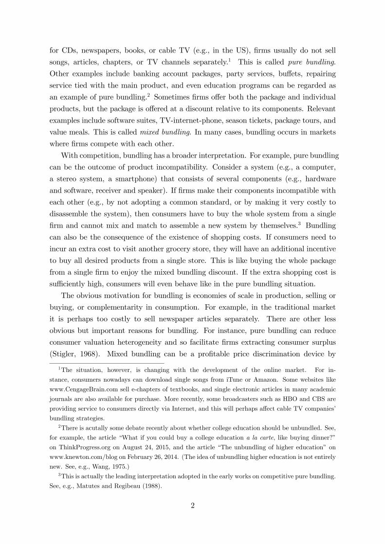
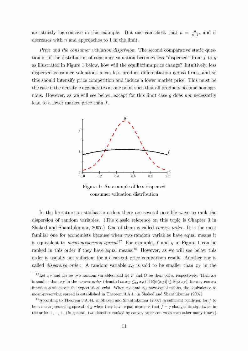
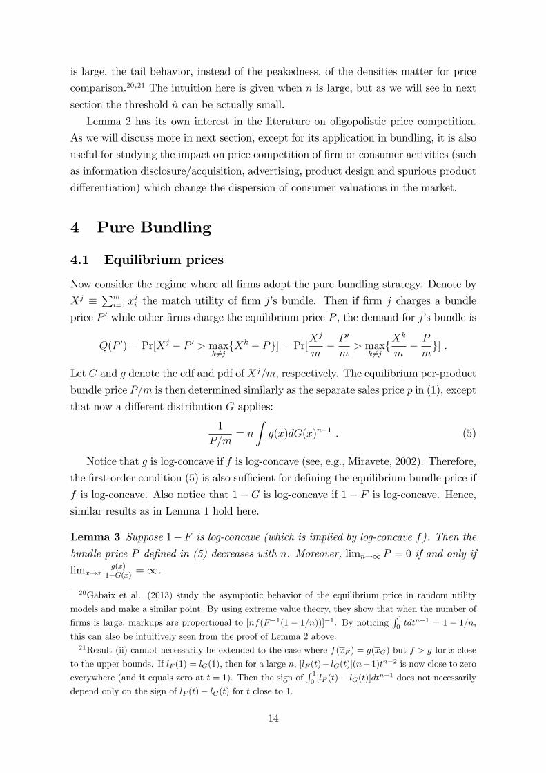
Price and the consumer valuation dispersion. The second comparative static ques-

tion is: if the distribution of consumer valuation becomes less �dispersed�from f to g

as illustrated in Figure 1 below, how will the equilibrium price change? Intuitively, less

dispersed consumer valuations mean less product di¤erentiation across �rms, and so

this should intensify price competition and induce a lower market price. This must be

the case if the density g degenerates at one point such that all products become homoge-

nous. However, as we will see below, except for this limit case g does not necessarily

lead to a lower market price than f .

0.0 0.2 0.4 0.6 0.8 1.00

1

2

f

x

g

Figure 1: An example of less dispersed

consumer valuation distribution

In the literature on stochastic orders there are several possible ways to rank the

dispersion of random variables. (The classic reference on this topic is Chapter 3 in

Shaked and Shanthikumar, 2007.) One of them is called convex order. It is the most

familiar one for economists because when two random variables have equal means it

is equivalent to mean-preserving spread.17 For example, f and g in Figure 1 can be

ranked in this order if they have equal means.18 However, as we will see below this

order is usually not su¢ cient for a clear-cut price comparison result. Another one is

called dispersive order. A random variable xG is said to be smaller than xF in the

17Let xF and xG be two random variables, and let F and G be their cdf�s, respectively. Then xGis smaller than xF in the convex order (denoted as xG �cx xF ) if E[�(xG)] � E[�(xF )] for any convexfunction � whenever the expectations exist. When xF amd xG have equal means, the equivalence to

mean-preserving spread is established in Theorem 3.A.1. in Shaked and Shanthikumar (2007).18According to Theorem 3.A.44. in Shaked and Shanthikumar (2007), a su¢ cient condition for f to

be a mean-preserving spread of g when they have equal means is that f � g changes its sign twice inthe order +;�;+. (In general, two densities ranked by convex order can cross each other many times.)

11

dispersive order (denoted as xG �disp xF ) if G�1(t) � G�1(t0) � F�1(t) � F�1(t0) for

any 0 < t0 � t < 1, where G and F are the cdf�s of xG and xF , respectively. (This

means that the di¤erence between any two quantiles of G is smaller than the di¤erence

between the corresponding quantiles of F .) This order will ensure a clear-cut price

comparison result as shown in the following result, but it is often a too strong condition

for the applications we will discuss below.19

Lemma 2 Consider two Perlo¤-Salop markets with consumer valuation xF and xG,

respectively. Let F and G be their cdf�s, f and g be their bounded pdf�s, and [xF ; xF ]

and [xG; xG] be their supports, respectively. Without loss of generality suppose E[xF ] =E[xG]. Let pk, k = F;G, be the equilibrium price associated with xk. Suppose both f

and g are log-concave such that the equilibrium prices are determined as in (1).

(i) If xG is less dispersed than xF according to the dispersive order, then pG � pF for

any n � 2.(ii) However, if f(xF ) > g(xG), then there exists n̂ such that pG > pF for n > n̂.

Proof. Changing the integral variable from x to t = F (x), we have

1

pF= n

Z xF

xF

f(x)dF (x)n�1 , 1

pF= n

Z 1

0

lF (t)dtn�1 ;

where lF (t) � f(F�1(t)) and tn�1 is a cdf on [0; 1]. Similarly, we have

1

pG= n

Z 1

0

lG(t)dtn�1 ;

where lG(t) � g(G�1(t)). Then

pG � pF ,Z 1

0

[lF (t)� lG(t)]dtn�1 � 0 : (4)

(i) xG �disp xF if and only if F�1(t) � G�1(t) increases in t 2 (0; 1). This impliesthat

dF�1(t)

dt� dG�1(t)

dt, f(F�1(t)) � g(G�1(t)) :

That is, lF (t) � lG(t). Therefore, pG � pF follows from (4).

(ii) lF (t)� lG(t) is bounded since both f and g are bounded. f(xF ) > g(xG) implies

lF (1)� lG(1) > 0. Then

limn!1

Z 1

0

[lF (t)� lG(t)]dtn�1 = lF (1)� lG(1) > 0

19When two random variables have equal means, dispersive order is a stronger condition than convex

order. (See Theorem 3.B.16. in Shaked and Shanthikumar, 2007.) Ganuza and Penalva (2010) use

these two orders to study information disclosure in auctions.

12

as the distribution tn�1 converges to the upper bound 1 as n ! 1. Then it followsfrom (4) that pG > pF when n is su¢ ciently large.

Result (i) shows that if one density is less dispersed than the other in the dispersive

order, the usual intuition works and we can predict that less dispersed consumer valu-

ations lead to a lower market price. Perlo¤ and Salop (1985) showed that if xG = �xF

with � 2 (0; 1), then pG < pF (more precisely, pG = �pF ). This is just a special case of

result (i) since �x �disp x for any random variable x and constant � 2 (0; 1). However,dispersive order is a relatively strong condition. When xF and xG have the same �nite

support, xG �disp xF requires F�1(t) � G�1(t) increase in t 2 (0; 1), but this impliesF�1(t) = G�1(t) everywhere. That is, the two random variables must be equal. This

excludes many natural cases where one random variable is intuitively more dispersed

than the other. For instance, the two distributions in Figure 1 cannot be ranked by

dispersive order. (When xF and xG have equal means and their supports are intervals,

xG �disp xF requires that the support of xG is a strict subset of the support of xF , orboth are in�nite supports.) For this reason, as we will see this order often does not help

in our bundling application.

Result (ii) shows that if we go beyond the dispersive order, even in natural cases

such as the example in Figure 1 where one distribution is less dispersed than the other,

the number of �rms can matter for price comparison. In particular, when there are

su¢ ciently many �rms in the market, a less dispersed distribution can lead to a higher

market price. When g is less dispersed than f , we usually perceive that g is more peaked

but has thinner tails as in Figure 1. So f(xF ) > g(xG) is a reasonable case to consider.

(From the proof of result (i) we know that this is not compatible with xG �disp xF .)Since this result is crucial for understanding our price comparison result in next section,

we explain its economic intuition in detail. Let us consider the example in Figure 1

where f(1) > g(1). From (2) we already know that equilibrium price equals the ratio

of equilibrium demand to the negative of equilibrium demand slope. Since equilibrium

demand is always 1=n due to �rm symmetry, only equilibrium demand slopes (or the

densities of marginal consumers) matter for the price comparison. When n is large, a

given consumer�s valuation for the best product among a �rm�s n � 1 competitors isclose to the upper bound 1 almost for sure. Therefore, for that consumer to be this

�rm�s marginal consumer, her valuation for its product should also be close to 1. In

other words, when n is large, the position of a �rm�s marginal consumers should be close

to the upper bound no matter which density function applies. Since f(1) > g(1), we

deduce that each �rm has fewer marginal consumers and so faces a less elastic demand

when the density g applies. Therefore, when n is large, the less dispersed density g

leads to a higher market price. This result suggests that when the number of �rms

13

is large, the tail behavior, instead of the peakedness, of the densities matter for price

comparison.20 ;21 The intuition here is given when n is large, but as we will see in next

section the threshold n̂ can be actually small.

Lemma 2 has its own interest in the literature on oligopolistic price competition.

As we will discuss more in next section, except for its application in bundling, it is also

useful for studying the impact on price competition of �rm or consumer activities (such

as information disclosure/acquisition, advertising, product design and spurious product

di¤erentiation) which change the dispersion of consumer valuations in the market.

4 Pure Bundling

4.1 Equilibrium prices

Now consider the regime where all �rms adopt the pure bundling strategy. Denote by

Xj �Pm

i=1 xji the match utility of �rm j�s bundle. Then if �rm j charges a bundle

price P 0 while other �rms charge the equilibrium price P , the demand for j�s bundle is

Q(P 0) = Pr[Xj � P 0 > maxk 6=j

fXk � Pg] = Pr[Xj

m� P 0

m> max

k 6=jfX

k

m� P

mg] :

Let G and g denote the cdf and pdf of Xj=m, respectively. The equilibrium per-product

bundle price P=m is then determined similarly as the separate sales price p in (1), except

that now a di¤erent distribution G applies:

1

P=m= n

Zg(x)dG(x)n�1 : (5)

Notice that g is log-concave if f is log-concave (see, e.g., Miravete, 2002). Therefore,

the �rst-order condition (5) is also su¢ cient for de�ning the equilibrium bundle price if

f is log-concave. Also notice that 1�G is log-concave if 1� F is log-concave. Hence,

similar results as in Lemma 1 hold here.

Lemma 3 Suppose 1�F is log-concave (which is implied by log-concave f). Then the

bundle price P de�ned in (5) decreases with n. Moreover, limn!1 P = 0 if and only if

limx!xg(x)

1�G(x) =1.

20Gabaix et al. (2013) study the asymptotic behavior of the equilibrium price in random utility

models and make a similar point. By using extreme value theory, they show that when the number of

�rms is large, markups are proportional to [nf(F�1(1 � 1=n))]�1. By noticingR 10tdtn�1 = 1 � 1=n,

this can also be intuitively seen from the proof of Lemma 2 above.21Result (ii) cannot necessarily be extended to the case where f(xF ) = g(xG) but f > g for x close

to the upper bounds. If lF (1) = lG(1), then for a large n, [lF (t)� lG(t)](n�1)tn�2 is now close to zeroeverywhere (and it equals zero at t = 1). Then the sign of

R 10[lF (t)� lG(t)]dtn�1 does not necessarily

depend only on the sign of lF (t)� lG(t) for t close to 1.

14

Notice that the per-product bundle valuationXj=m is a mean-preserving contraction

of xji and they have the same support.22 So g is less dispersed than f as illustrated

in Figure 1 above. In particular, g(x) = 0 even if f(x) > 0. This is simply because

Xj=m = x only if xji = x for all i = 1; � � � ;m, or intuitively this is because �nding awell matched bundle is much harder than �nding a well matched single product.23

4.2 Comparing prices and pro�ts

From (1) and (5), we can see that the comparison between separate sales and pure

bundling is just a comparison between two Perlo¤-Salop models with di¤erent match

utility distributions F and G. According to result (i) in Lemma 2, bundling reduces

market price if Xj=m �disp xji . However, Xj=m and xji usually cannot be ranked by

the dispersive order. This is the case as we pointed out before if xji has a �nite support.

Given the further restriction here that Xj=m and xji share the same support and mean

(which means that F and G must cross each other at least once), this is also the case if

xji has a semi-in�nite support with a �nite lower or upper bound. The only case where

Xj=m �disp xji might hold is when the support of xji is the whole real line. One such

example is the normal distribution as we will discuss more later. The following result

indicates that bundling leads to lower prices in duopoly even if Xj=m and xji are not

ranked by the dispersive order, but if we go beyond duopoly it will be often the case

that bundling raises market price if the number of �rms is large enough.

Using the technique in the proof of Lemma 2, we have

P

m� p,

Z 1

0

[lF (t)� lG(t)]tn�2dt � 0 ; (6)

where lF (t) = f(F�1(t)) and lG(t) = g(G�1(t)). Given full market coverage, pro�t

comparison is the same as price comparison.

Proposition 1 Suppose f is log-concave. (i) When n = 2, bundling reduces market

prices and pro�ts for any m � 2.(ii) For a �xed m, if f is bounded and f(x) > 0, there exists n̂ such that bundling

increases market prices and pro�ts for n > n̂. If f is further such that lF (t) and lG(t)

cross each other at most twice, then bundling decreases prices and pro�ts if and only if

n � n̂.

(iii) For a �xed n, P increases inm at a speed ofpm whenm is large and limm!1 P=m =

0, so there exists m̂ such that bundling reduces market prices and pro�ts for m > m̂.

22This is true as long as the mean of xji exists. See, for example, p. 127 in Shaked and Shanthikumar

(2007) for a formal proof.23Formally, when m = 2 the pdf of (xj1 + x

j2)=2 is g(x) = 2

R x2x�x f(2x� t)dF (t) for x � (x+ x)=2,

so g(x) = 0. A similar argument works for m � 3.

15

Result (i) generalizes the observation in the existing literature on how pure bundling

a¤ects market prices in duopoly. Bundling reduces price in duopoly ifRf(x)2dx �R

g(x)2dx. The intuition of this result is more transparent when the density function f

is symmetric. In that case, the average position of marginal consumers is at the mean,

and g is more peaked at the mean than f . Thus, there are more marginal consumers

(and so the demand is more elastic) in the case of g.24 This induces �rms to charge a

lower price in the bundling regime. In Lemma 2, we did not �nd a simple stochastic

order condition beyond dispersive order which ensures pG � pF when n = 2. This is

an open question in general, but result (i) here suggests that this is the case if xG is a

sample mean of xF .

Result (iii) follows from the law of large numbers. Given the assumption that xjihas a �nite mean �, Xj=m converges to � as m!1. In other words, the per-productvaluation for the bundle becomes homogeneous across both consumers and �rms. Then

P=m must converge to zero.25

Result (ii) that pure bundling can soften price competition is perhaps more surpris-

ing. The result for large n follows from result (ii) in Lemma 2 since f(x) > g(x) = 0.

Bundling makes the (per-product) valuation density have a thinner right tail, and when

n is large the marginal consumers mainly locate on the right tail. In other words,

bundling reduces the number of marginal consumers. This leads to a less elastic de-

mand and a higher market price. The cut-o¤ result is, however, harder to prove.26

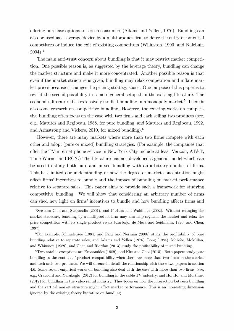
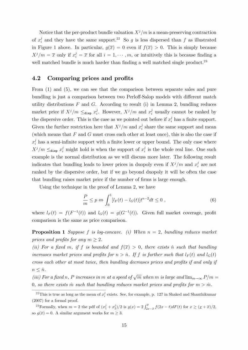
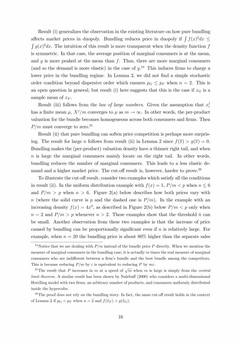
To illustrate the cut-o¤result, consider two examples which satisfy all the conditions

in result (ii). In the uniform distribution example with f(x) = 1, P=m < p when n � 6and P=m > p when n > 6. Figure 2(a) below describes how both prices vary with

n (where the solid curve is p and the dashed one is P=m). In the example with an

increasing density f(x) = 4x3, as described in Figure 2(b) below P=m < p only when

n = 2 and P=m > p whenever n > 2. These examples show that the threshold n̂ can

be small. Another observation from these two examples is that the increase of price

caused by bundling can be proportionally signi�cant even if n is relatively large. For

example, when n = 20 the bundling price is about 80% higher than the separate sales

24Notice that we are dealing with P=m instead of the bundle price P directly. When we mention the

measure of marginal consumers in the bundling case, it is actuallym times the real measure of marginal

consumers who are indi¤erent between a �rm�s bundle and the best bundle among the competitors.

This is because reducing P=m by " is equivalent to reducing P by m".25The result that P increases in m at a speed of

pm when m is large is simply from the central

limit theorem. A similar result has been shown by Nalebu¤ (2000) who considers a multi-dimensional

Hotelling model with two �rms, an arbitrary number of products, and consumers uniformly distributed

inside the hypercube.26The proof does not rely on the bundling story. In fact, the same cut-o¤ result holds in the context

of Lemma 2 if pG < pF when n = 2 and f(xF ) > g(xG).

16

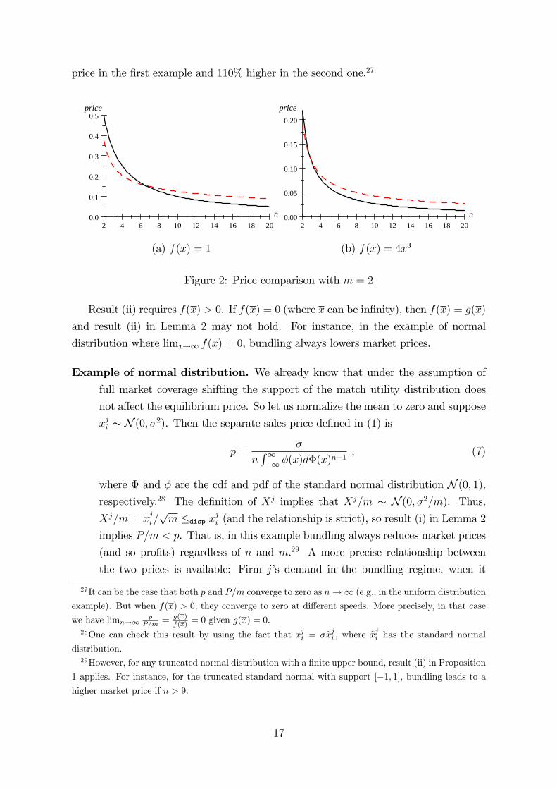
price in the �rst example and 110% higher in the second one.27

2 4 6 8 10 12 14 16 18 200.0

0.1

0.2

0.3

0.4

0.5price

n

(a) f(x) = 1

2 4 6 8 10 12 14 16 18 200.00

0.05

0.10

0.15

0.20

price

n

(b) f(x) = 4x3

Figure 2: Price comparison with m = 2

Result (ii) requires f(x) > 0. If f(x) = 0 (where x can be in�nity), then f(x) = g(x)

and result (ii) in Lemma 2 may not hold. For instance, in the example of normal

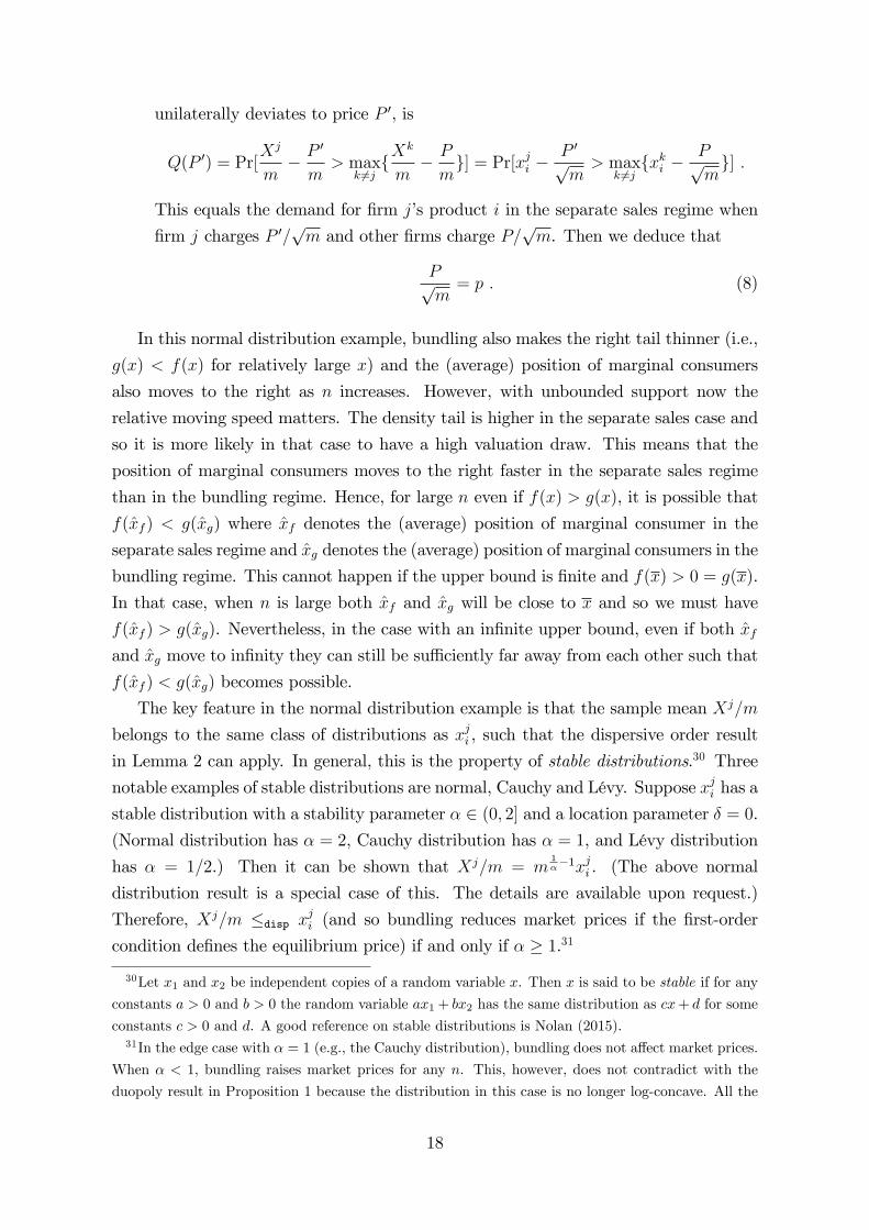
distribution where limx!1 f(x) = 0, bundling always lowers market prices.

Example of normal distribution. We already know that under the assumption offull market coverage shifting the support of the match utility distribution does

not a¤ect the equilibrium price. So let us normalize the mean to zero and suppose

xji s N (0; �2). Then the separate sales price de�ned in (1) is

p =�

nR1�1 �(x)d�(x)

n�1 ; (7)

where � and � are the cdf and pdf of the standard normal distribution N (0; 1),respectively.28 The de�nition of Xj implies that Xj=m s N (0; �2=m). Thus,Xj=m = xji=

pm �disp xji (and the relationship is strict), so result (i) in Lemma 2

implies P=m < p. That is, in this example bundling always reduces market prices

(and so pro�ts) regardless of n and m.29 A more precise relationship between

the two prices is available: Firm j�s demand in the bundling regime, when it

27It can be the case that both p and P=m converge to zero as n!1 (e.g., in the uniform distribution

example). But when f(x) > 0, they converge to zero at di¤erent speeds. More precisely, in that case

we have limn!1p

P=m = g(x)f(x) = 0 given g(x) = 0.

28One can check this result by using the fact that xji = �~xji , where ~xji has the standard normal

distribution.29However, for any truncated normal distribution with a �nite upper bound, result (ii) in Proposition

1 applies. For instance, for the truncated standard normal with support [�1; 1], bundling leads to ahigher market price if n > 9.

17

unilaterally deviates to price P 0, is

Q(P 0) = Pr[Xj

m� P 0

m> max

k 6=jfX

k

m� P

mg] = Pr[xji �

P 0pm> max

k 6=jfxki �

Ppmg] :

This equals the demand for �rm j�s product i in the separate sales regime when

�rm j charges P 0=pm and other �rms charge P=

pm. Then we deduce that

Ppm= p : (8)

In this normal distribution example, bundling also makes the right tail thinner (i.e.,

g(x) < f(x) for relatively large x) and the (average) position of marginal consumers

also moves to the right as n increases. However, with unbounded support now the

relative moving speed matters. The density tail is higher in the separate sales case and

so it is more likely in that case to have a high valuation draw. This means that the

position of marginal consumers moves to the right faster in the separate sales regime

than in the bundling regime. Hence, for large n even if f(x) > g(x), it is possible that

f(x̂f ) < g(x̂g) where x̂f denotes the (average) position of marginal consumer in the

separate sales regime and x̂g denotes the (average) position of marginal consumers in the

bundling regime. This cannot happen if the upper bound is �nite and f(x) > 0 = g(x).

In that case, when n is large both x̂f and x̂g will be close to x and so we must have

f(x̂f ) > g(x̂g). Nevertheless, in the case with an in�nite upper bound, even if both x̂fand x̂g move to in�nity they can still be su¢ ciently far away from each other such that

f(x̂f ) < g(x̂g) becomes possible.

The key feature in the normal distribution example is that the sample mean Xj=m

belongs to the same class of distributions as xji , such that the dispersive order result

in Lemma 2 can apply. In general, this is the property of stable distributions.30 Three

notable examples of stable distributions are normal, Cauchy and Lévy. Suppose xji has a

stable distribution with a stability parameter � 2 (0; 2] and a location parameter � = 0.(Normal distribution has � = 2, Cauchy distribution has � = 1, and Lévy distribution

has � = 1=2.) Then it can be shown that Xj=m = m1��1xji . (The above normal

distribution result is a special case of this. The details are available upon request.)

Therefore, Xj=m �disp xji (and so bundling reduces market prices if the �rst-ordercondition de�nes the equilibrium price) if and only if � � 1.31

30Let x1 and x2 be independent copies of a random variable x. Then x is said to be stable if for any

constants a > 0 and b > 0 the random variable ax1 + bx2 has the same distribution as cx+ d for some

constants c > 0 and d. A good reference on stable distributions is Nolan (2015).31In the edge case with � = 1 (e.g., the Cauchy distribution), bundling does not a¤ect market prices.

When � < 1, bundling raises market prices for any n. This, however, does not contradict with the

duopoly result in Proposition 1 because the distribution in this case is no longer log-concave. All the

18

Another example in which bundling always reduces market price is the exponential

distribution. Although the dispersive order argument does not work any more, there

is an alternative way to compare the prices. We already know that as the exponential

distribution has a constant hazard rate, the separate sales price p in this example

is independent of n. While Xj=m, the per-product valuation for the bundle, has a

strictly log-concave density, so P=m strictly decreases in n. We know from result (i) in

Proposition 1 that in this example bundling reduces market price in duopoly. Then we

can deduce that it must be the case for any n � 2.However, these examples do not suggest that f(x) > 0 (or a �nite x) is necessary for

the result that bundling can raise market price. For instance, consider the distribution

with a log-concave density f(x) = 2(1 � x) and support x 2 [0; 1]. In this example,f(x) = 0 but numerical simulations suggest a similar price comparison result as in

Figure 2 (though the threshold n̂ becomes bigger). There are also examples with x =1and a log-concave density where bundling can raise market price. For instance, consider

the generalized normal distribution with density f(x) = �2�(1=�)

e�jxj�

, where � is the

shape parameter and the support is the whole real line. (The density function is log-

concave when � > 1.) This distribution becomes the standard normal when � = 2,

and it converges to the uniform distribution on [�1; 1] when � !1. Suppose n̂ is thethreshold in the case of uniform distribution with support [�1; 1]. Then for any n > n̂,

there exists su¢ ciently large � such that bundling raises market price.

Other possible applications. There are many other �rm or consumer activities (such

as information disclosure, advertising, product design, and consumer information ac-

quisition) which can also change the dispersion of consumer valuations in a similar way

as bundling. Our results in Lemma 2 and Proposition 1 can o¤er useful insights about

how those activities might a¤ect price competition.32

Here we brie�y discuss a model of spurious product di¤erentiation (in the spirit of

Spiegler, 2006) which is isomorphic to our model. Suppose �rms sell a homogenous

product, and all consumers have an identical valuation u for this product. Consumers

discussion here is subject to the quali�cation that for some stable distributions the �rst-order condition

may not be su¢ cient for de�ning the equilibrium price, or the integral in the �rst-order condition may

not even exist.32There are works that study �rms�individual incentive to disclose product information or conduct

other activities that change the dispersion of consumer valuations. Lewis and Sappington (1994) and

Johnson and Myatt (2006) consider a monopoly model and show that the �rm will provide either

full or zero information. Ivanov (2013) extends Johnson and Myatt (2006) and studies equilibrium

information disclosure in an oligopoly model with price competition. He focuses on investigating when

full information disclosure is an equilibrium and shows that this is the case when the number of �rms

is su¢ ciently large. But he does not study how the change of consumer valuation dispersion a¤ects

market prices and welfare.

19

do not know this true valuation, but they can independently observe m noisy signals

(x1; � � � ; xm). Suppose each signal xi is an independent draw from a continuous distrib-ution with mean u. Suppose consumers are non-Bayesian and they take the average face

values of the signals, 1m

Pmi=1 xi, as the true valuation for the product. (Spiegler, 2006,

considers the case with m = 1 and a binary signal realization.) Here the non-Bayesian

behavior of consumers causes arti�cial product di¤erentiation among �rms such that

the market price is above the cost. When m increases, the distribution of consumer

valuation will become more concentrated around the true valuation u. In particular, if

m!1 consumers will eventually �nd out the true valuation, and market competition

will drive the markup down to zero. Therefore, in this model we can regard m as an

index of consumer rationality. Our price comparison results suggest that whether or

not higher consumer rationality intensi�es competition often depends on the number

of �rms in the market. In particular, beyond the duopoly case an improvement of

consumer rationality can actually relax price competition and harm consumers.

4.3 Comparing consumer surplus and total welfare

With full market coverage, consumer payment is a pure transfer and so total welfare

(which is the sum of �rm pro�ts and consumer surplus) only re�ects the match quality

between consumers and products. In either regime, price is the same across �rms in

a symmetric equilibrium and so it does not distort consumer choices. Since bundling

eliminates the opportunity to mix and match for consumers, it must reduce match

quality and so total welfare.

However, the comparison of consumer surplus can be more complicated. If pure

bundling increases market prices, it must harm consumers. From Proposition 1, we

know this is the case when f(x) > 0 and n is su¢ ciently large. The trickier situation

is when pure bundling lowers market prices (e.g., when n = 2, m is large, or the

distribution is normal or exponential). Then there is a trade-o¤ between the negative

match quality e¤ect and the positive price e¤ect. The main message in this section

is that even if bundling intensi�es price competition, the negative match quality e¤ect

often dominates such that bundling harms consumers when the number of �rms is above

a usually small threshold.

The per-product consumer surplus in the regime of separate sales and the regime of

bundling are respectively

E�maxjfxjig

�� p and E

�maxj

�Xj

m

��� P

m:

Then bundling bene�ts consumers if and only if

E�maxjfxjig

�� E

�maxj

�Xj

m

��< p� P

m: (9)

20

The left-hand side (which must be positive) re�ects the match quality e¤ect and the

right-hand side is the price e¤ect.

The following proposition reports the analytical results we have for consumer surplus

comparison.

Proposition 2 Suppose f is log-concave. (i) For a �xed m, if f is bounded and f(x) >0, or if limx!x

ddx(1�F (x)f(x)

) = 0, there exists n̂ such that bundling harms consumers if

n > n̂.

(ii) There exists n� such that (a) for n � n�, there exists m̂(n) such that bundling

bene�ts consumers if m > m̂(n), and (b) for n > n�, there exists m̂(n) such that

bundling harms consumers if m > m̂(n).

The �rst condition in result (i) follows the price comparison result (ii) in Proposition

1, and it requires a �nite x. When x =1 the second condition covers many often used

distributions such as normal, exponential, extreme value, and logistic. Intuitively, this

is because when x = 1 the di¤erence between E�maxjfxjig

�and E

hmaxj

nXj

m

oican

go to in�nity as n ! 1, while the price di¤erence is always �nite since both pricesdecrease with n under the log-concavity condition.

Result (ii) says that in the limit case with m ! 1 a stronger cut-o¤ result is

available: pure bundling improves consumer welfare if and only if the number of

�rms is below some threshold. Notice that in the limit case with m ! 1 we have

limm!1Xj=m = � and limm!1 P=m = 0. Then for �xed n, bundling bene�ts con-

sumers if and only if

E�maxjfxjig

�� � < p : (10)

It is clear that the match quality e¤ect increases with n (because with more �rms

bundling eliminates more mixing-and-matching opportunities), while the price e¤ect

decreases with n. What we show in the proof is that (10) holds for n = 2 but fails for a

su¢ ciently large n. This leads to the cut-o¤ result. The threshold n� is typically small.

For example, in the uniform distribution case with F (x) = x, condition (10) simpli�es

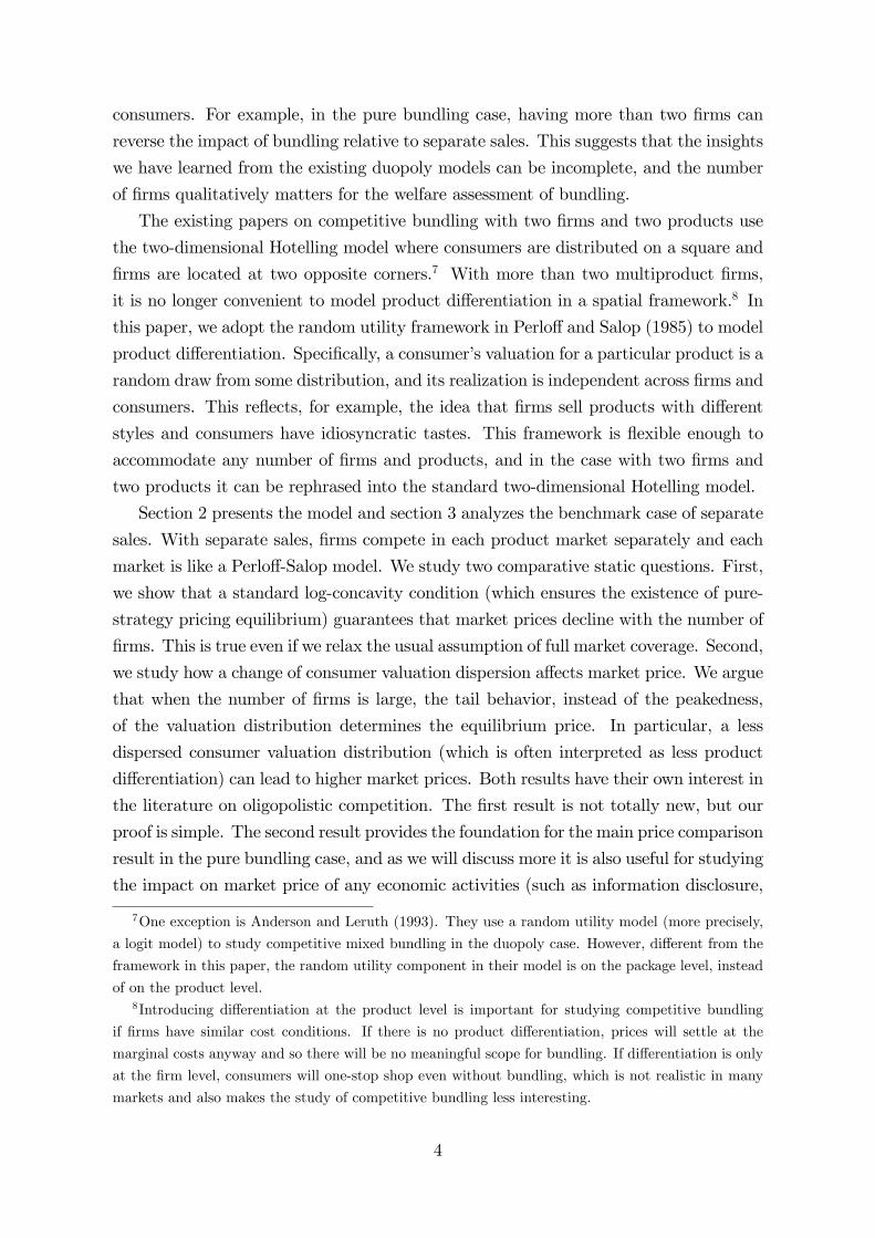
to n2 � 3n� 2 < 0, which holds only for n � 3.For a smallm, it appears di¢ cult to prove a cut-o¤result.33 Figure 3 below describes

how consumer surplus varies with n in the uniform distribution case whenm = 2 (where

the solid curve is for separate sales, and the dashed one is for bundling). Again, the

threshold is n� = 3. The graph also suggests that the harm of bundling on consumers

can be signi�cant (e.g., when n = 10, bundling reduces consumer surplus by about

33We have examples where bundling harms consumers even in the duopoly case. One such example

is when m = 2 and the distribution is exponential.

21

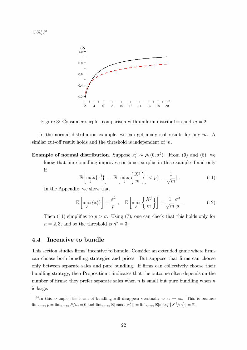
15%).34

2 4 6 8 10 12 14 16 18 20

0.2

0.4

0.6

0.8

1.0

n

CS

Figure 3: Consumer surplus comparison with uniform distribution and m = 2

In the normal distribution example, we can get analytical results for any m. A

similar cut-o¤ result holds and the threshold is independent of m.

Example of normal distribution. Suppose xji s N (0; �2). From (9) and (8), we

know that pure bundling improves consumer surplus in this example if and only

if

E�maxjfxjig

�� E

�maxj

�Xj

m

��< p[1� 1p

m] : (11)

In the Appendix, we show that

E�maxjfxjig

�=�2

p; E

�maxj

�Xj

m

��=

1pm

�2

p: (12)

Then (11) simpli�es to p > �. Using (7), one can check that this holds only for

n = 2; 3, and so the threshold is n� = 3.

4.4 Incentive to bundle

This section studies �rms�incentive to bundle. Consider an extended game where �rms

can choose both bundling strategies and prices. But suppose that �rms can choose

only between separate sales and pure bundling. If �rms can collectively choose their

bundling strategy, then Proposition 1 indicates that the outcome often depends on the

number of �rms: they prefer separate sales when n is small but pure bundling when n

is large.

34In this example, the harm of bundling will disappear eventually as n ! 1. This is becauselimn!1 p = limn!1 P=m = 0 and limn!1 E[maxjfxjig] = limn!1 E[maxj

�Xj=m

] = x.

22

The outcome is di¤erent if �rms choose their bundling strategies non-cooperatively.

We mainly focus on the case where �rms choose bundling strategies and prices simulta-

neously. This captures the situations where it is relatively easy to adjust the bundling

strategy.

Proposition 3 Suppose f is log-concave and �rms make bundling and pricing decisionssimultaneously.

(i) It is a Nash equilibrium that all �rms choose to bundle their products and charge

the bundle price P de�ned in (5). When n = 2, this is the unique (pure-strategy) Nash

equilibrium if p 6= P=m.

(ii) There exists ~n such that (a) for n � ~n, there exists ~m(n) such that separate sales

is not a Nash equilibrium if m > ~m(n), and (b) for n > ~n, there exists ~m(n) such that

separate sales is also a Nash equilibrium if m > ~m(n).

It is easy to understand that all �rms bundling is a Nash equilibrium. This is

simply because in our model if a �rm unilaterally unbundles the market situation does

not change for consumers.35 In the duopoly case, it can be further shown that separate

sales cannot be an equilibrium outcome, and there are also no asymmetric equilibria

where one �rm bundles and the other does not.

When there are more than two �rms, one may wonder whether separate sales can

become another equilibrium outcome. Result (ii) says that when m ! 1, this is thecase if and only if n is above some threshold. The intuition of why the number of �rms

matters is that the more �rms in the market, the more inferior a �rm�s bundle appears

when it unilaterally bundles while its rivals do not. (This is di¤erent from the argument

in the duopoly case where one �rm bundling forces the other �rm to bundle as well.)

More formally, suppose that all other �rms o¤er separate sales at price p, but �rm j

unilaterally bundles. Denote by

yi � maxk 6=j

fxki g (13)

the maximum match utility of product i among �rm j�s competitors. Then �rm j is

as if competing with one �rm that o¤ers a bundle with match utility Y �Pm

i=1 yi and

price mp. If �rm j charges the same bundle price mp, its demand will be Pr(Xj >

Y ) � Pr(Xj > maxk 6=jfXkg) = 1=n. The inequality is strict for n � 3. Thus, withoutfurther price adjustment it cannot be pro�table for �rm j to unilaterally bundle.

Suppose now �rm j can also adjust its price. It is more convenient to rephrase

the problem into a monopoly one where a consumer�s net valuation for product i is

ui � xi � (yi � p). (Here yi � p can be regarded as the outside option to product i.) If

35This argument depends on the assumption that consumers buy all products but for each product

they do not buy more than one variant.

23

�rm j does not bundle, then its optimal separate sales price is p and its pro�t from each

product is p=n. But its optimal pro�t when it bundles is hard to calculate in general,

except for the limit case with m!1.36 In the limit case, according to the law of largenumbers �rm j can extract all surplus by charging a bundle price m�E[ui] and its perproduct pro�t will be E[ui] = �� E[yi] + p. This is no greater than the separate sales

pro�t if and only if

(1� 1

n)p < E[yi]� � =

Z �F (x)� F (x)n�1

�dx : (14)

This is clearly not true for n = 2 (which is consistent with result (i)). In the proof, we

show that this is true if and only if n is above a certain threshold.

The threshold ~n in result (ii) is usually small. For instance, with a uniform distri-

bution (14) becomes n2 � 4n + 2 > 0 and so ~n = 3. This is the same as the thresholdn� in the consumer surplus comparison result in Proposition 2. This means that in this

uniform example with a large number of products, separate sales is another equilibrium

outcome if and only if consumers prefer separate sales to pure bundling. In other words,

with a proper equilibrium selection the market can work well for consumers. This is

also true for the exponential and the normal distribution.37

Asymmetric equilibrium. With more than two �rms one may also wonder the pos-

sibility of asymmetric equilibrium where some �rms bundle and the others do not. An

analytical investigation into this problem is hard because the pricing equilibrium when

�rms adopt asymmetric bundling strategies does not have a simple characterization.38

However, numerical analysis can be done. Let us illustrate by a uniform example with

n = 3 andm = 2. In this example, we can claim that there are no asymmetric equilibria.

The �rst possible asymmetric equilibrium is that one �rm bundles and the other

36This simplicity of optimal pricing with many products has been explored by Armstrong (1999)

and Bakos and Brynjolfsson (1999). Fang and Norman (2006) have studied the pro�tability of pure

bundling in the monopoly case with a �nite number of products. They assume that the density of

ui is log-concave and symmetric. In our model, the log-concavity is guaranteed if f is log-concave,

but the density of ui is not symmetric when n � 3 (because yi is stochastically greater than xi).

Without symmetry, the Proschan (1965) result thatPm

i=1 ui=m is more peaked than ui does not hold

any more. (The Proschan (1965) result has been extended in various ways, but not when the density

is asymmetric.) The analysis in Fang and Norman (2006), however, relies on that result. That is why

we cannot apply their results to our model.37However, there exist examples (e.g., f(x) = 2(1� x)) where ~n 6= n�.38The reason is that the �rms which bundle their products make each other �rm treats their products

as complements. This complicates the demand calculation. To understand this, let us suppose �rm 1

bundles while other �rms do not. When �rm k 6= 1 lowers its product i�s price, some consumers willstop buying �rm 1�s bundle and switch to buying all products from other �rms. This will increase the

demand for �rm k�s all products. (The details on the demand calculation and the �rst-order conditions

are available upon request, but no further analytical progress can be made.)

24

two do not. In this hypothetical equilibrium, the bundling �rm charges P � 0:513 andearns a pro�t about 0:176, and the other two �rms charge a separate price p � 0:317and each earns a pro�t about 0:208. But if the bundling �rm unbundles and charges

the same separate price as the other two �rms, it will have a demand 13and its pro�t

will rise to about 0:211. The second possible asymmetric equilibrium is that two �rms

bundle and the third one does not. This hypothetical equilibrium is like all �rm are

bundling. Then each bundling �rm charges a bundle price P = 0:5, the third �rm

charges p1 + p2 = 0:5, and each �rm has market share 13. But if one bundling �rm

unbundles and o¤ers the same separate prices as the third �rm, as we already knew

the remaining bundling �rm will have a demand less than 13, and this implies that the

deviation �rm will have a demand greater than 13. This improves its pro�t.

Sequential choices. Suppose now that �rms make their bundling choices �rst, and

then engage in price competition after observing the bundling outcome. First of all, as

before all �rms bundling is a Nash equilibrium outcome. The issue of whether separate

sales is also an equilibrium is more complicated. In the duopoly case, if f is log-concave,

then bundling leads to a lower price and pro�t as we have shown in Proposition 1. Then

no �rm has a unilateral incentive to deviate from separate sales. That is, separate sales

is a Nash equilibrium outcome as well.

When there are more than two �rms, due to the complication of the pricing game

when �rms adopt asymmetric bundling strategies, no general results are available. In

the uniform example with n = 3 and m = 2, we can numerically show that separate

sales is another equilibrium, but there are no asymmetric equilibria. If all three �rms

sell their products separately, each �rm charges a price p = 13and each �rm�s pro�t is

29� 0:222. Now if one �rm, say, �rm 1 deviates and bundles, then in the asymmetric

pricing game, �rm 1 charges a bundle price P � 0:513 and the other two �rms chargea separate price p � 0:317 for each product. Firm 1�s pro�t drops to about 0:176 (and

each other �rm�s pro�t drops to about 0:208). So no �rm wants to bundle unilaterally.

This also implies that one �rm bundling and the other two not is not an equilibrium,

because all �rms bene�t if the bundling �rm unbundles. The last possibility is that two

�rms bundle and the other does not. That situation is like all �rms bundling, and each

�rm�s pro�t is about 0:167. But if one bundling �rm unbundles, its pro�t will rise to

0:208. Hence, there are no asymmetric equilibria.

4.5 Discussions

4.5.1 Asymmetric products and correlated distributions

We now consider a more general setting where the m products within each �rm are

potentially asymmetric and their match utilities are potentially correlated. Let xj =

25

(xj1; � � � ; xjm) be a consumer�s valuations for the m products at �rm j. Suppose xj is

still i.i.d. across �rms and consumers, and it is distributed according to a common joint

cdf F (x1; � � � ; xm) with support S � Rm and a continuous joint pdf f(x1; � � � ; xm). LetFi and fi, i = 1; � � � ;m, be the marginal cdf and pdf of xji , and let [xi; xi] be its support.Let G and g be the cdf and pdf of Xj=m, the average per-product match utility of the

bundle, and let [x; x] be its support. All fi and g are log-concave if the joint pdf f is

log-concave.

In the regime of separate sales, since competition is still separate across products,

the equilibrium price for product i is determined the same as in formula (1) as long as

we use the corresponding marginal distribution:

1

pi= n

Z xi

xi

fi(x)dFi(x)n�1 :

In the regime of pure bundling, the average per-product bundle price is still determined

as in (5):1

P=m=

Z x

x

g(x)dG(x)n�1 :

The limit result that limm!1 P=m = 0 still holds as long as Xj=m converges to a

deterministic value as m!1. So for a �xed n, bundling lowers market price when mis su¢ ciently large. Under similar conditions as before, we also have the result that for

a �xed m bundling raises market prices when n is su¢ ciently large.

Proposition 4 Suppose f is continuous, bounded and log-concave. Suppose S � Rm

is compact, strictly convex, and has full dimension. Then for a �xed m,

(i) if fi(xi) > 0, there exists n̂i such that P=m > pi for n > n̂i;

(ii) if fi(xi) > 0 for all i = 1; � � � ;m, there exists n̂ such that P >Pm

i=1 pi for n > n̂.

Proof. Our conditions imply that g(x) = 0 (e.g., see the proof of Proposition 1 inArmstrong, 1996).39 Then the results immediately follow from Lemma 2.

The previous normal distribution example can also be extended to this general case.

Suppose xj � N (0;�), where �2i in� is the variance of xji and �ik in� is the covariance

of (xji ; xjk). Then X

j=m � N (0; (Pm

i=1 �2i +

Pi6=k �ik)=m

2). According to formula (7),

P <Pm

i=1 pi if and only ifPm

i=1 �2i +

Pi6=k �ik < (

Pmi=1 �i)

2. Given �ik � �i�k for

any i 6= k, this condition must hold provided that at least one pair of (xji ; xjk) are not

perfectly correlated.

39More formally, g(x) = lim"!01�G(x�")

" , and our conditions ensure 1�G(x�") = o("). Among theconditions, strict convexity of S excludes the possibility that the plane of Xj=m = x coincides with

some part of S�s boundary, and S being of full dimension excludes the possibility that xji , i = 1; � � � ;m,are perfectly correlated.

26

What is less clear is whether bundling still lowers market price in the duopoly case.

Following the logic in the proof of result (i) in Proposition 1, let hi be the pdf of

x1i � x2i . (Notice that x1i � x2i is symmetric around zero, and hi is log-concave if fi

is log-concave.) Then the separate sales price for product i is pi = 12hi(0)

. Let �h be

the pdf of 1m

Pmi=1(x

1i � x2i ). Then the per-product bundle price is P=m = 1

2�h(0), and

P <Pm

i=1 pi if and only if1�h(0)

<1

m

mXi=1

1

hi(0): (15)

Jensen�s Inequality implies that the right-hand side is greater than�1m

Pmi=1 hi(0)

��1.

Therefore, a su¢ cient condition for P <Pm

i=1 pi is

1

m

mXi=1

hi(0) � �h(0) : (16)

Unfortunately, we are unable to �nd simple primitive conditions on the joint pdf f such

that (15) or (16) is satis�ed.40 The following example shows that in the duopoly case

bundling can still lower market price even if products are substantially asymmetric.

Example of asymmetric products. Consider a two-product example where xj1 isuniformly distributed on [0; 1] and xj2 is independent of x

j1 and is uniformly dis-

tributed on [0; b] with b > 1. In duopoly, x11 � x21 and x12 � x22 have pdf�s

h1(x) =

(1 + x if x 2 [�1; 0]1� x if x 2 [0; 1]

and h2(x) =

(1b(1 + x

b) if x 2 [�b; 0]

1b(1� x

b) if x 2 [0; b]

;

respectively. Then h1(0) = 1 and h2(0) = 1b. One can also check �h(0) = 2(3b�1)

3b2.

The su¢ cient condition (16) holds only for b less than about 2:46, but the �i¤�

condition (15) holds for any b > 1. Hence, bundling lowers prices in duopoly.

However, according to Proposition 4 bundling will raise prices in this example

when n is su¢ ciently large.

4.5.2 Without full market coverage

We now return to the symmetric and independent case but relax the assumption of full

market coverage. (The analysis below, though, can be extended to the general setup as

40If the m products are symmetric and the joint pdf of fx1i � x2i gmi=1 is Schur-concave, or if them products at each �rm have independent match utilities and any two random variables x1i � x2i andx1k�x2k can be ranked according to the likelihood ratio order, then there are extensions of the Proschan(1956) result which can help prove (16). But we do not have simple primitive conditions for either of

the conditions to hold. (In the symmetric and independent case, both conditions are satis�ed if f is

log-concave.)

27

in the previous section.) A subtle issue here is whether the m products are independent

products or perfect complements. This will a¤ect the analysis in the separate sales

benchmark. If the m products are independent products, consumers decide whether to

buy each product separately. While if the m products are perfect complements, then

whether to buy a certain product also depends on how well matched other products

are. (With full market coverage, this distinction does not matter.) In the following, we

consider the case of independent products for simplicity.

Suppose now xji denotes the whole valuation for �rm j�s product i, and a consumer

will buy a product or bundle only if the best o¤er in the market provides a positive

surplus. To make the case interesting, let us suppose x � 0 but � > 0, such that someconsumers do not buy but the whole market is still active.

In the regime of separate sales, if �rm j deviates and charges p0 for its product i,

then the demand for its product i is

q(p0) = Pr[xji � p0 > maxk 6=j

f0; xki � pg] =Z x

p0F (xji � p0 + p)n�1dF (xji ) :

One can check that the �rst-order condition for p to be the equilibrium price is

p =q(p)

jq0(p)j =[1� F (p)n]=n

F (p)n�1f(p)| {z }exclusion e¤ect

+

Z x

p

f(x)dF (x)n�1| {z }competition e¤ect

: (17)

(If f is log-concave, this is also su¢ cient for de�ning the equilibrium price.) In equilib-

rium, a consumer will leave the market without purchasing product i with probability

F (p)n (i.e., when each product i has a valuation less than p). Given the symmetry of

�rms, the numerator in (17) is the demand for each �rm�s product i in equilibrium.

The denominator is the negative of the demand slope but it now has two parts: (i)

The �rst term is the standard market exclusion e¤ect: when the valuations of all other

�rms�product i are below p (which occurs with probability F (p)n�1), �rm j will play

as a monopoly. Then raising its price p by " will exclude "f(p) consumers from the

market. (ii) The second term is the same competition e¤ect as in the case with full

market coverage (up to the adjustment that a marginal consumer�s valuation must be

greater than the price p).

Similarly, in the bundling case the equilibrium per-product price P=m is determined

by the �rst-order condition:

P

m=

[1�G(P=m)n]=n

G(P=m)n�1g(P=m) +R xP=m

g(x)dG(x)n�1; (18)

where G and g are the cdf and pdf of Xj=m as before.

28

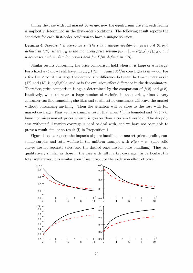
Unlike the case with full market coverage, now the equilibrium price in each regime

is implicitly determined in the �rst-order conditions. The following result reports the

condition for each �rst-order condition to have a unique solution.

Lemma 4 Suppose f is log-concave. There is a unique equilibrium price p 2 (0; pM)de�ned in (17), where pM is the monopoly price solving pM = [1� F (pM)]=f(pM), and

p decreases with n. Similar results hold for P=m de�ned in (18).

Similar results concerning the price comparison hold when m is large or n is large.

For a �xed n <1, we still have limm!1 P=m = 0 sinceXj=m converges asm!1. Fora �xed m <1, if n is large the demand size di¤erence between the two numerators in(17) and (18) is negligible, and so is the exclusion e¤ect di¤erence in the denominators.

Therefore, price comparison is again determined by the comparison of f(x) and g(x).

Intuitively, when there are a large number of varieties in the market, almost every

consumer can �nd something she likes and so almost no consumers will leave the market

without purchasing anything. Then the situation will be close to the case with full

market coverage. Thus we have a similar result that when f(x) is bounded and f(x) > 0,

bundling raises market prices when n is greater than a certain threshold. The duopoly

case without full market coverage is hard to deal with, and we have not been able to

prove a result similar to result (i) in Proposition 1.

Figure 4 below reports the impacts of pure bundling on market prices, pro�ts, con-

sumer surplus and total welfare in the uniform example with F (x) = x. (The solid

curves are for separate sales, and the dashed ones are for pure bundling.) They are

qualitatively similar as those in the case with full market coverage. In particular, the

total welfare result is similar even if we introduce the exclusion e¤ect of price.

2 4 6 8 100.0

0.1

0.2

0.3

0.4

n

price

2 4 6 8 100.0

0.1

0.2

0.3

n

profit

2 4 6 8 100.2

0.3

0.4

0.5

0.6

0.7

0.8

n

CS

2 4 6 8 100.5

0.6

0.7

0.8

0.9

n

W

29

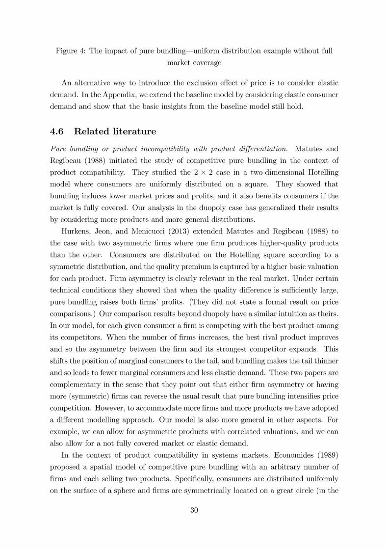
Figure 4: The impact of pure bundling� uniform distribution example without full

market coverage

An alternative way to introduce the exclusion e¤ect of price is to consider elastic

demand. In the Appendix, we extend the baseline model by considering elastic consumer

demand and show that the basic insights from the baseline model still hold.

4.6 Related literature

Pure bundling or product incompatibility with product di¤erentiation. Matutes and

Regibeau (1988) initiated the study of competitive pure bundling in the context of

product compatibility. They studied the 2 � 2 case in a two-dimensional Hotellingmodel where consumers are uniformly distributed on a square. They showed that

bundling induces lower market prices and pro�ts, and it also bene�ts consumers if the

market is fully covered. Our analysis in the duopoly case has generalized their results

by considering more products and more general distributions.

Hurkens, Jeon, and Menicucci (2013) extended Matutes and Regibeau (1988) to

the case with two asymmetric �rms where one �rm produces higher-quality products

than the other. Consumers are distributed on the Hotelling square according to a

symmetric distribution, and the quality premium is captured by a higher basic valuation

for each product. Firm asymmetry is clearly relevant in the real market. Under certain

technical conditions they showed that when the quality di¤erence is su¢ ciently large,

pure bundling raises both �rms�pro�ts. (They did not state a formal result on price

comparisons.) Our comparison results beyond duopoly have a similar intuition as theirs.

In our model, for each given consumer a �rm is competing with the best product among

its competitors. When the number of �rms increases, the best rival product improves

and so the asymmetry between the �rm and its strongest competitor expands. This

shifts the position of marginal consumers to the tail, and bundling makes the tail thinner

and so leads to fewer marginal consumers and less elastic demand. These two papers are

complementary in the sense that they point out that either �rm asymmetry or having

more (symmetric) �rms can reverse the usual result that pure bundling intensi�es price

competition. However, to accommodate more �rms and more products we have adopted

a di¤erent modelling approach. Our model is also more general in other aspects. For

example, we can allow for asymmetric products with correlated valuations, and we can

also allow for a not fully covered market or elastic demand.

In the context of product compatibility in systems markets, Economides (1989)

proposed a spatial model of competitive pure bundling with an arbitrary number of

�rms and each selling two products. Speci�cally, consumers are distributed uniformly

on the surface of a sphere and �rms are symmetrically located on a great circle (in the

30

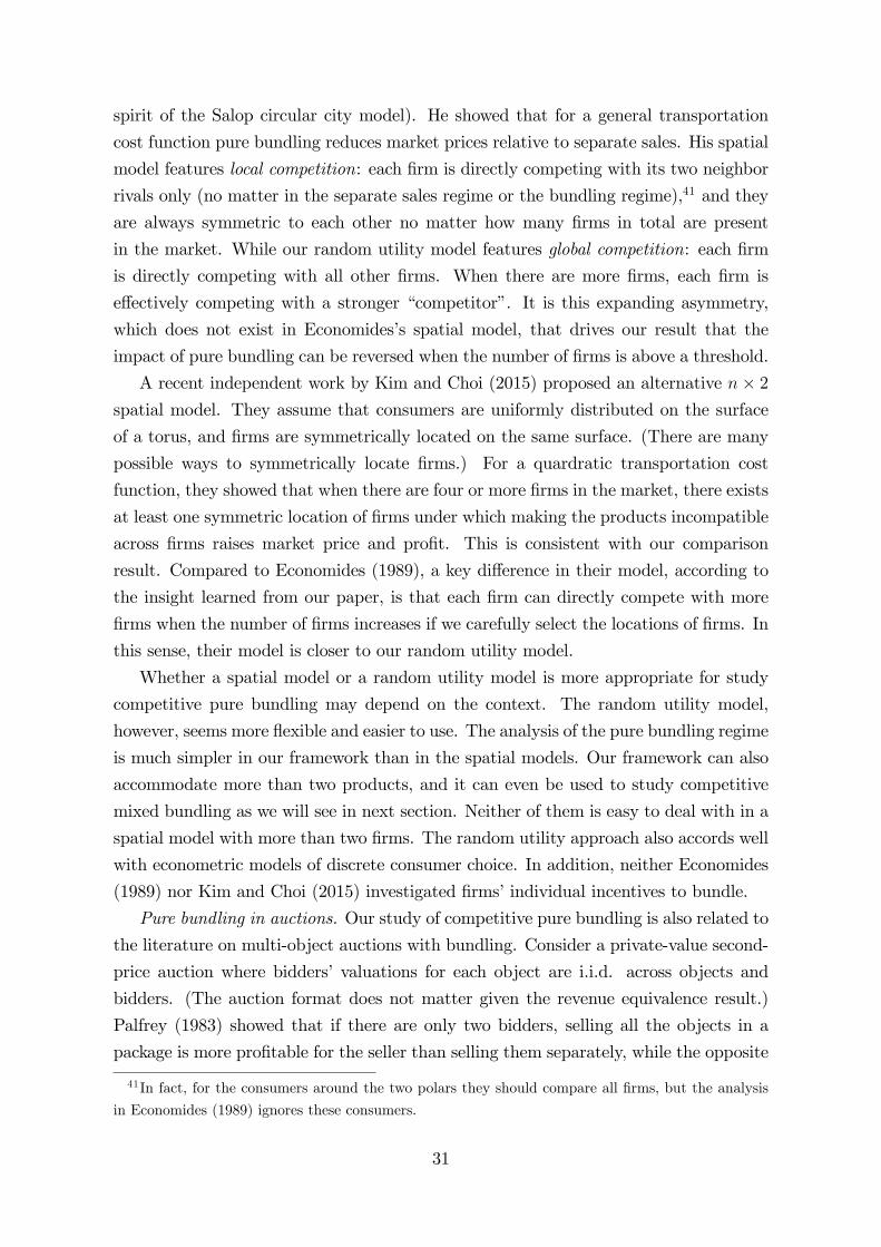
spirit of the Salop circular city model). He showed that for a general transportation

cost function pure bundling reduces market prices relative to separate sales. His spatial

model features local competition: each �rm is directly competing with its two neighbor

rivals only (no matter in the separate sales regime or the bundling regime),41 and they

are always symmetric to each other no matter how many �rms in total are present

in the market. While our random utility model features global competition: each �rm

is directly competing with all other �rms. When there are more �rms, each �rm is

e¤ectively competing with a stronger �competitor�. It is this expanding asymmetry,

which does not exist in Economides�s spatial model, that drives our result that the

impact of pure bundling can be reversed when the number of �rms is above a threshold.

A recent independent work by Kim and Choi (2015) proposed an alternative n� 2spatial model. They assume that consumers are uniformly distributed on the surface

of a torus, and �rms are symmetrically located on the same surface. (There are many

possible ways to symmetrically locate �rms.) For a quardratic transportation cost

function, they showed that when there are four or more �rms in the market, there exists

at least one symmetric location of �rms under which making the products incompatible

across �rms raises market price and pro�t. This is consistent with our comparison

result. Compared to Economides (1989), a key di¤erence in their model, according to

the insight learned from our paper, is that each �rm can directly compete with more

�rms when the number of �rms increases if we carefully select the locations of �rms. In

this sense, their model is closer to our random utility model.

Whether a spatial model or a random utility model is more appropriate for study

competitive pure bundling may depend on the context. The random utility model,

however, seems more �exible and easier to use. The analysis of the pure bundling regime

is much simpler in our framework than in the spatial models. Our framework can also

accommodate more than two products, and it can even be used to study competitive

mixed bundling as we will see in next section. Neither of them is easy to deal with in a

spatial model with more than two �rms. The random utility approach also accords well

with econometric models of discrete consumer choice. In addition, neither Economides

(1989) nor Kim and Choi (2015) investigated �rms�individual incentives to bundle.

Pure bundling in auctions. Our study of competitive pure bundling is also related to

the literature on multi-object auctions with bundling. Consider a private-value second-

price auction where bidders�valuations for each object are i.i.d. across objects and

bidders. (The auction format does not matter given the revenue equivalence result.)

Palfrey (1983) showed that if there are only two bidders, selling all the objects in a

package is more pro�table for the seller than selling them separately, while the opposite

41In fact, for the consumers around the two polars they should compare all �rms, but the analysis

in Economides (1989) ignores these consumers.

31

is true when the number of bidders is su¢ ciently large. The revenue from selling the

objects separately is equal to the sum of the second highest valuations for each product.

While the revenue from selling them together in a bundle is equal to the second highest

valuation for the bundle. With only two bidders the second highest valuation is the

minimum valuation, so the revenue must be higher in the bundling case. With many

bidders, however, the second highest valuation is close to the maximum valuation, so

the revenue must be higher with separate sales. (In this limit bidders�information rent

disappears and so only the allocation e¢ ciency matters for the revenue, and bundling

clearly reduces allocation e¢ ciency.) In the two-object case, Chakraborty (1999) further

showed a cut-o¤ result under certain regularity conditions.

Notice that the seller in an auction is like consumers in our price competition model,

and the agents on the other side of the market are competing for them. Hence, revenue

comparison in auctions is related to consumer surplus comparison (instead of price and

pro�t comparison) in our model. The analysis in an auction model does not directly

apply to our price competition model. Competition occurs on the informed side in

auctions but on the uninformed side in our price competition model. In the auction

model, since we can focus on the second-price auction, the equilibrium bidding strategy

is simple and all analysis can be based on the order statistic of the second highest

valuation. While in our model as we have seen in (3) the equilibrium price is related

to the second order statistic in a more complex way. This makes our analysis less

straightforward than in the auction case. This also partially explains, for example,

why revenue comparison in auctions with two or many bidders is very general but its

counterpart, i.e., consumer surplus comparison, in our model is less so.42

Pure bundling with homogenous products and heterogeneous costs. In the literature

on competitive bundling, to make bundling a meaningful issue to study the standard

approach is to consider a market with horizontal production di¤erentiation. We have

followed that tradition, though we have adopted a random utility model instead of a

spatial one. There is, however, an alternative modelling approach which considers homo-

geneous products with heterogeneous costs across �rms. A simple setting is to assume

that consumers have the identical valuation for all products but the unit production

cost is i.i.d. across �rms and products, and each �rm has private cost realizations. Since

competition now occurs on the informed side, the situation is like a �rst-price procure-

42As we pointed out before in the end of section 4.2, product information disclosure can a¤ect

consumer valuation distribution in a similar way as pure bundling. The same analogy applies in the

auction case. Among the works which study information disclosure in auctions, Board (2009) and

Ganuza and Penalva (2010) are the two most related papers. Both of them showed that whether

or not the auctioneer bene�ts from publicly providing more information to bidders depends on the

number of bidders as in the above auction papers. Board (2009) pointed out the connection between

bundling and information disclosure.

32

ment auction. Since the outcome is the same as in a second-price auction, the above

argument for auctions implies that consumers must bene�t from bundling in duopoly

but su¤er when there are many �rms. Given total welfare is always lower with bundling,

we can deduce that �rms must su¤er from bundling in the duopoly case. When the

number of �rms is su¢ ciently large, as in result (ii) of Proposition 1 we can show that

the opposite is true if the cost density function is strictly positive at the lower bound.

Farrell, Monroe, and Saloner (1998) is a related paper in this direction. They

compare pro�tability of two forms of vertical organization of industry: open organi-

zation (which can be interpreted as separate sales) vs closed organization (which can

be interpreted as pure bundling). The di¤erence is that they assume a Bertrand price

competition among �rms with public cost information. Then the �rm with the lowest

cost wins the whole market and charges a price equal to the second lowest cost. From

the ex ante perspective, this setting generates the same outcome as in the private cost

setting. In the n� 2 case they show a similar pro�t comparison result.

5 Mixed Bundling

In this section, we study competitive mixed bundling. All the existing research on

competitive mixed bundling focuses on the duopoly case. See, for example, Matutes

and Regibeau (1992), Anderson and Leruth (1993), Thanassoulis (2007), and Armstrong

and Vickers (2010). Armstrong and Vickers (2010) considered the most general setup

so far in the literature: they allow for asymmetric products and correlated valuations,

and they also consider elastic demand and a general nonlinear pricing schedule. This

paper is the �rst to consider the case with more than two �rms. As we will see below,

solving the mixed bundling pricing game becomes much harder when we go beyond the

duopoly case. One contribution of this paper is to propose a way to solve the problem,

and when the number of �rms is large we also show that the equilibrium prices have

relatively simple approximations.

For tractability, we focus on the baseline model with full market coverage. We also

assume that each �rm supplies two products only and they have i.i.d. match utilities.43

If a �rm adopts a mixed bundling strategy, it o¤ers a pair of stand-alone prices (�1; �2)

and a joint-purchase discount � > 0. (Then if a consumer buys both products from

this �rm, she pays �1 + �2 � �.) In the following, we will �rst argue that starting

from separate sales with price p de�ned in (1), each �rm has a unilateral incentive to

introduce mixed bundling. We will then characterize the symmetric pricing equilibrium

43It is not di¢ cult to extend the analysis below to the case with asymmetric products and correlated

valuations. Dealing with the case with more than two products is more di¢ cult because of the resulted

complication of the pricing strategy space.

33

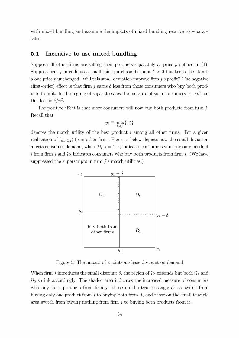
with mixed bundling and examine the impacts of mixed bundling relative to separate

sales.

5.1 Incentive to use mixed bundling

Suppose all other �rms are selling their products separately at price p de�ned in (1).

Suppose �rm j introduces a small joint-purchase discount � > 0 but keeps the stand-

alone price p unchanged. Will this small deviation improve �rm j�s pro�t? The negative

(�rst-order) e¤ect is that �rm j earns � less from those consumers who buy both prod-

ucts from it. In the regime of separate sales the measure of such consumers is 1=n2, so

this loss is �=n2.

The positive e¤ect is that more consumers will now buy both products from �rm j.

Recall that

yi � maxk 6=j

fxki g

denotes the match utility of the best product i among all other �rms. For a given

realization of (y1; y2) from other �rms, Figure 5 below depicts how the small deviation

a¤ects consumer demand, where i, i = 1; 2, indicates consumers who buy only product

i from �rm j and b indicates consumers who buy both products from �rm j. (We have

suppressed the superscripts in �rm j�s match utilities.)

x1

x2

y2

y1

b2

1

y1 � �

y2 � �

ppppppppppppppppppppp

ppppppppppppppppppppp

ppppppppppppppppppppp ppppppppppppppppppppp pppppppppppppppppppp pppppppppppppppppppppbuy both fromother �rms

Figure 5: The impact of a joint-purchase discount on demand

When �rm j introduces the small discount �, the region of b expands but both 1 and

2 shrink accordingly. The shaded area indicates the increased measure of consumers

who buy both products from �rm j: those on the two rectangle areas switch from

buying only one product from j to buying both from it, and those on the small triangle

area switch from buying nothing from �rm j to buying both products from it.

34

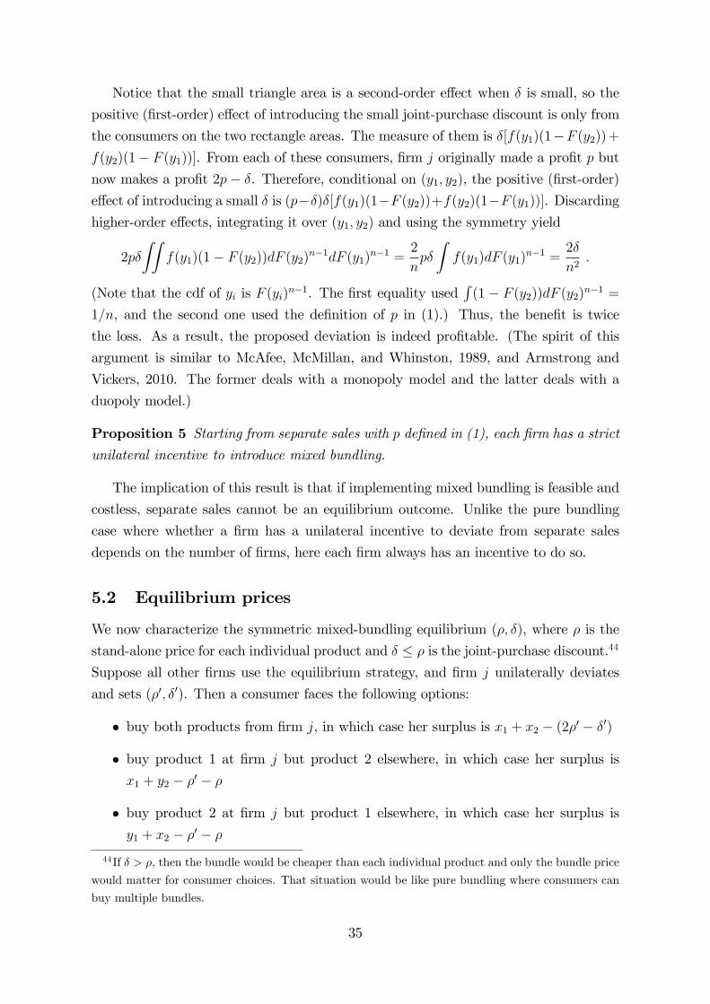
Notice that the small triangle area is a second-order e¤ect when � is small, so the

positive (�rst-order) e¤ect of introducing the small joint-purchase discount is only from

the consumers on the two rectangle areas. The measure of them is �[f(y1)(1�F (y2))+f(y2)(1� F (y1))]. From each of these consumers, �rm j originally made a pro�t p but

now makes a pro�t 2p� �. Therefore, conditional on (y1; y2), the positive (�rst-order)

e¤ect of introducing a small � is (p��)�[f(y1)(1�F (y2))+f(y2)(1�F (y1))]. Discardinghigher-order e¤ects, integrating it over (y1; y2) and using the symmetry yield

2p�

ZZf(y1)(1� F (y2))dF (y2)

n�1dF (y1)n�1 =

2

np�

Zf(y1)dF (y1)

n�1 =2�

n2:

(Note that the cdf of yi is F (yi)n�1. The �rst equality usedR(1 � F (y2))dF (y2)

n�1 =

1=n, and the second one used the de�nition of p in (1).) Thus, the bene�t is twice

the loss. As a result, the proposed deviation is indeed pro�table. (The spirit of this

argument is similar to McAfee, McMillan, and Whinston, 1989, and Armstrong and

Vickers, 2010. The former deals with a monopoly model and the latter deals with a

duopoly model.)

Proposition 5 Starting from separate sales with p de�ned in (1), each �rm has a strictunilateral incentive to introduce mixed bundling.

The implication of this result is that if implementing mixed bundling is feasible and

costless, separate sales cannot be an equilibrium outcome. Unlike the pure bundling

case where whether a �rm has a unilateral incentive to deviate from separate sales

depends on the number of �rms, here each �rm always has an incentive to do so.

5.2 Equilibrium prices

We now characterize the symmetric mixed-bundling equilibrium (�; �), where � is the

stand-alone price for each individual product and � � � is the joint-purchase discount.44

Suppose all other �rms use the equilibrium strategy, and �rm j unilaterally deviates

and sets (�0; �0). Then a consumer faces the following options:

� buy both products from �rm j, in which case her surplus is x1 + x2 � (2�0 � �0)

� buy product 1 at �rm j but product 2 elsewhere, in which case her surplus is

x1 + y2 � �0 � �

� buy product 2 at �rm j but product 1 elsewhere, in which case her surplus is

y1 + x2 � �0 � �

44If � > �, then the bundle would be cheaper than each individual product and only the bundle price

would matter for consumer choices. That situation would be like pure bundling where consumers can

buy multiple bundles.

35

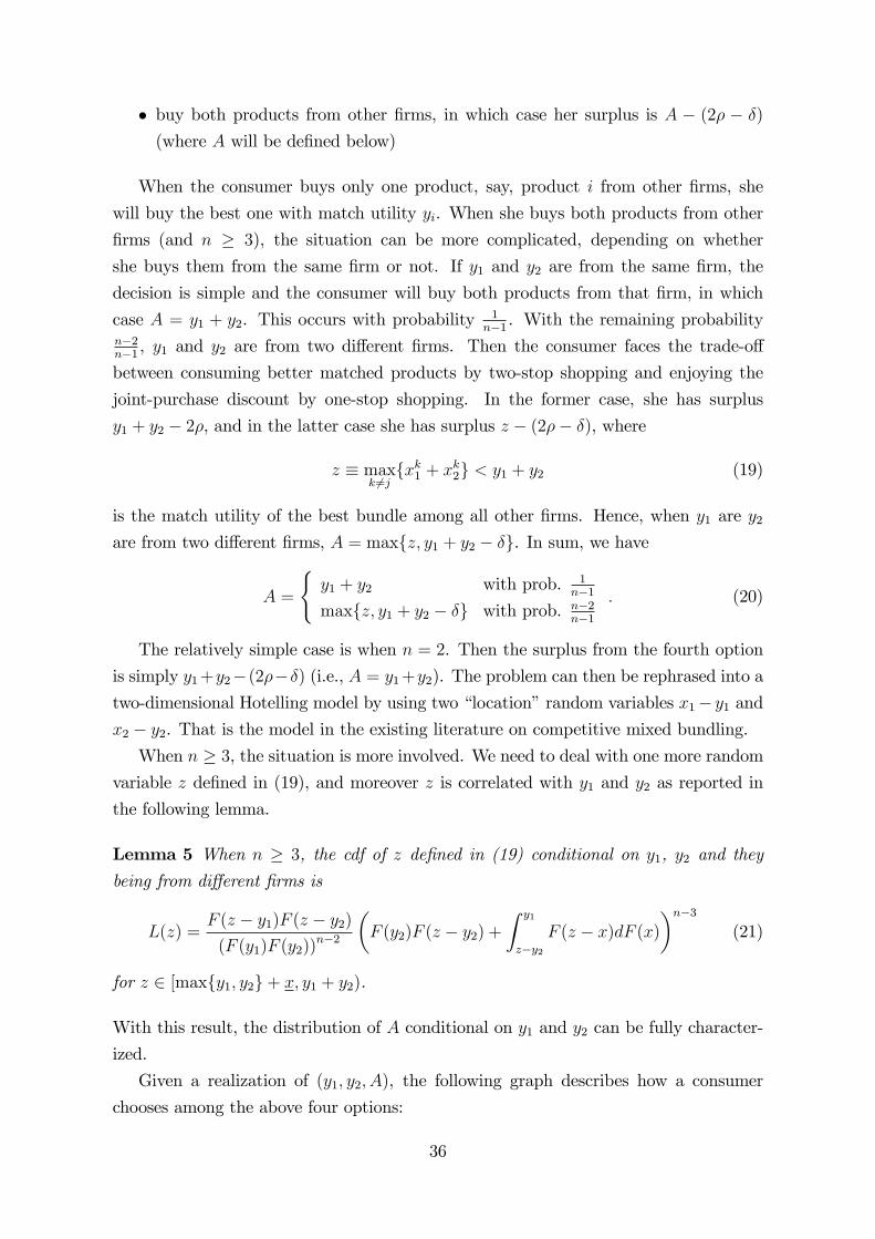
� buy both products from other �rms, in which case her surplus is A � (2� � �)

(where A will be de�ned below)

When the consumer buys only one product, say, product i from other �rms, she

will buy the best one with match utility yi. When she buys both products from other

�rms (and n � 3), the situation can be more complicated, depending on whether

she buys them from the same �rm or not. If y1 and y2 are from the same �rm, the

decision is simple and the consumer will buy both products from that �rm, in which

case A = y1 + y2. This occurs with probability 1n�1 . With the remaining probability

n�2n�1 , y1 and y2 are from two di¤erent �rms. Then the consumer faces the trade-o¤

between consuming better matched products by two-stop shopping and enjoying the

joint-purchase discount by one-stop shopping. In the former case, she has surplus

y1 + y2 � 2�, and in the latter case she has surplus z � (2�� �), where

z � maxk 6=j

fxk1 + xk2g < y1 + y2 (19)

is the match utility of the best bundle among all other �rms. Hence, when y1 are y2are from two di¤erent �rms, A = maxfz; y1 + y2 � �g. In sum, we have

A =

(y1 + y2 with prob. 1

n�1maxfz; y1 + y2 � �g with prob. n�2

n�1: (20)

The relatively simple case is when n = 2. Then the surplus from the fourth option

is simply y1+y2�(2���) (i.e., A = y1+y2). The problem can then be rephrased into a

two-dimensional Hotelling model by using two �location�random variables x1� y1 andx2 � y2. That is the model in the existing literature on competitive mixed bundling.

When n � 3, the situation is more involved. We need to deal with one more randomvariable z de�ned in (19), and moreover z is correlated with y1 and y2 as reported in

the following lemma.

Lemma 5 When n � 3, the cdf of z de�ned in (19) conditional on y1, y2 and they

being from di¤erent �rms is

L(z) =F (z � y1)F (z � y2)

(F (y1)F (y2))n�2

�F (y2)F (z � y2) +

Z y1

z�y2F (z � x)dF (x)

�n�3(21)

for z 2 [maxfy1; y2g+ x; y1 + y2).

With this result, the distribution of A conditional on y1 and y2 can be fully character-

ized.

Given a realization of (y1; y2; A), the following graph describes how a consumer

chooses among the above four options:

36

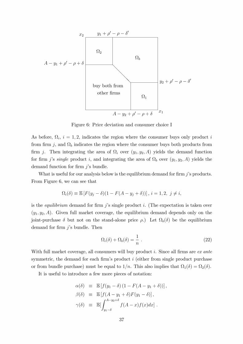
x1

x2

@@@@@

y1 + �0 � �� �0

A� y2 + �0 � �+ �

y2 + �0 � �� �0

A� y1 + �0 � �+ �b

2

1

buy both from

other �rms

Figure 6: Price deviation and consumer choice I

As before, i, i = 1; 2, indicates the region where the consumer buys only product i

from �rm j, and b indicates the region where the consumer buys both products from

�rm j. Then integrating the area of i over (y1; y2; A) yields the demand function

for �rm j�s single product i, and integrating the area of b over (y1; y2; A) yields the

demand function for �rm j�s bundle.

What is useful for our analysis below is the equilibrium demand for �rm j�s products.

From Figure 6, we can see that

i(�) � E [F (yj � �)(1� F (A� yj + �))] , i = 1; 2; j 6= i;

is the equilibrium demand for �rm j�s single product i. (The expectation is taken over

(y1; y2; A). Given full market coverage, the equilibrium demand depends only on the

joint-purchase � but not on the stand-alone price �.) Let b(�) be the equilibrium

demand for �rm j�s bundle. Then

i(�) + b(�) =1

n: (22)

With full market coverage, all consumers will buy product i. Since all �rms are ex ante

symmetric, the demand for each �rm�s product i (either from single product purchase

or from bundle purchase) must be equal to 1=n. This also implies that 1(�) = 2(�).

It is useful to introduce a few more pieces of notation:

�(�) � E [f(y1 � �) (1� F (A� y1 + �))] ;

�(�) � E [f(A� y1 + �)F (y1 � �)] ;

(�) � E[Z A�y2+�

y1��f(A� x)f(x)dx] :

37

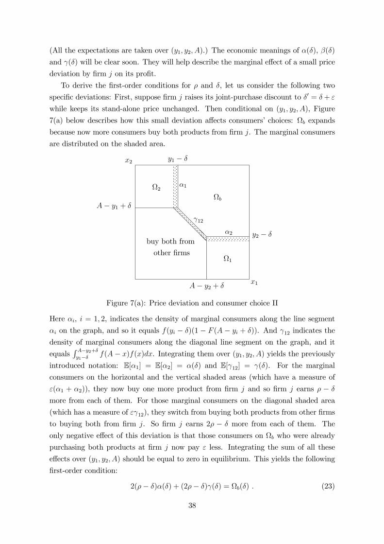
(All the expectations are taken over (y1; y2; A).) The economic meanings of �(�), �(�)

and (�) will be clear soon. They will help describe the marginal e¤ect of a small price

deviation by �rm j on its pro�t.

To derive the �rst-order conditions for � and �, let us consider the following two

speci�c deviations: First, suppose �rm j raises its joint-purchase discount to �0 = �+ "

while keeps its stand-alone price unchanged. Then conditional on (y1; y2; A), Figure

7(a) below describes how this small deviation a¤ects consumers�choices: b expands

because now more consumers buy both products from �rm j. The marginal consumers

are distributed on the shaded area.

x1

x2

@@@@@

y1 � �

A� y2 + �

y2 � �

A� y1 + �b

2

1

buy both from

other �rms

pppppppppppppp

pppppppppppppppppppppppppppppp pppppppppppppp

@@@@@@

p p p p p p p p p p p p p p pp p p p p p p p p p p p p p

12

�1

�2

Figure 7(a): Price deviation and consumer choice II

Here �i, i = 1; 2, indicates the density of marginal consumers along the line segment

�i on the graph, and so it equals f(yi � �)(1 � F (A � yi + �)). And 12 indicates the

density of marginal consumers along the diagonal line segment on the graph, and it

equalsR A�y2+�y1�� f(A� x)f(x)dx. Integrating them over (y1; y2; A) yields the previously

introduced notation: E[�1] = E[�2] = �(�) and E[ 12] = (�). For the marginal

consumers on the horizontal and the vertical shaded areas (which have a measure of

"(�1 + �2)), they now buy one more product from �rm j and so �rm j earns � � �

more from each of them. For those marginal consumers on the diagonal shaded area

(which has a measure of " 12), they switch from buying both products from other �rms

to buying both from �rm j. So �rm j earns 2� � � more from each of them. The

only negative e¤ect of this deviation is that those consumers on b who were already

purchasing both products at �rm j now pay " less. Integrating the sum of all these

e¤ects over (y1; y2; A) should be equal to zero in equilibrium. This yields the following

�rst-order condition:

2(�� �)�(�) + (2�� �) (�) = b(�) : (23)

38

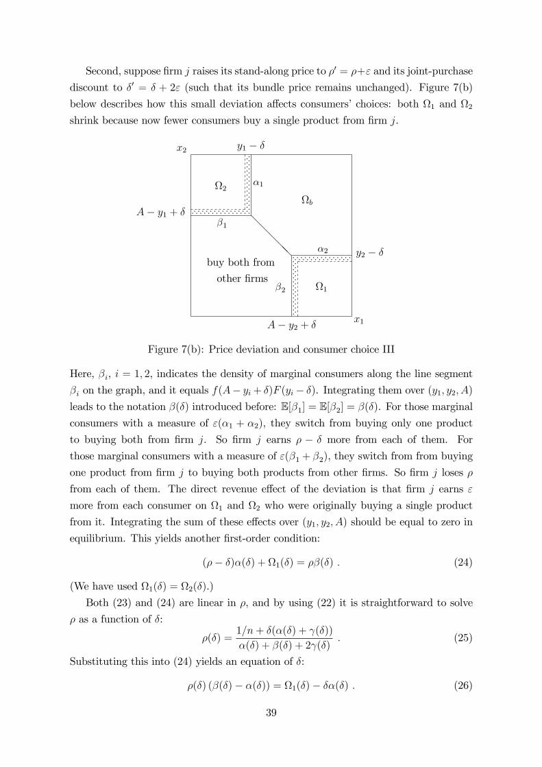
Second, suppose �rm j raises its stand-along price to �0 = �+" and its joint-purchase

discount to �0 = � + 2" (such that its bundle price remains unchanged). Figure 7(b)

below describes how this small deviation a¤ects consumers�choices: both 1 and 2shrink because now fewer consumers buy a single product from �rm j.

x1

x2

@@@@@

y1 � �

A� y2 + �

y2 � �

A� y1 + �b

2

1

buy both from

other �rms

p p p p p p p p p p p p p pp p p p p p p p p p p p p

pppppppppppppp

ppppppppppppppp

pppppppppppppp

pppppppppppppp ppppppppppppppp ppppppppppppp

�1

�2

�1

�2

Figure 7(b): Price deviation and consumer choice III

Here, �i, i = 1; 2, indicates the density of marginal consumers along the line segment

�i on the graph, and it equals f(A� yi + �)F (yi� �). Integrating them over (y1; y2; A)

leads to the notation �(�) introduced before: E[�1] = E[�2] = �(�). For those marginal

consumers with a measure of "(�1 + �2), they switch from buying only one product

to buying both from �rm j. So �rm j earns � � � more from each of them. For

those marginal consumers with a measure of "(�1 + �2), they switch from from buying

one product from �rm j to buying both products from other �rms. So �rm j loses �

from each of them. The direct revenue e¤ect of the deviation is that �rm j earns "

more from each consumer on 1 and 2 who were originally buying a single product

from it. Integrating the sum of these e¤ects over (y1; y2; A) should be equal to zero in

equilibrium. This yields another �rst-order condition:

(�� �)�(�) + 1(�) = ��(�) : (24)

(We have used 1(�) = 2(�).)

Both (23) and (24) are linear in �, and by using (22) it is straightforward to solve

� as a function of �:

�(�) =1=n+ �(�(�) + (�))

�(�) + �(�) + 2 (�): (25)

Substituting this into (24) yields an equation of �:

�(�) (�(�)� �(�)) = 1(�)� ��(�) : (26)

39

Discussion: equilibrium existence. To prove the existence of a symmetric (pure-

strategy) equilibrium,45 we need to show (i) the system of (25) and (26) has a solution

with � < �, and (ii) the �rst-order conditions are su¢ cient for de�ning the equilibrium.

Unfortunately, both conditions are hard to investigate in general. For the �rst one,

we can show it when n = 2 or when n is su¢ ciently large. For the second one, little

analytical progress can be made. This issue exists even in the duopoly case (except

for some speci�c distributions) and is an unsolved problem in the literature on mixed

bundling in general. Numerically we can show that the existence is not a problem in

the uniform distribution and the normal distribution example.46

The complication of (25) and (26) comes from the fact that �(�), �(�), (�) and

1(�) usually do not have simple expressions. However, they are simple in the duopoly

case, and they also have relatively simple approximations when � is small (which, as we

will show below, is often the case when the number of �rms is large). Hence, we study

these two cases in the following.

For convenience, let H(�) be the cdf of xi � yi. Then

H(t) =

Z x

x

F (x+ t)dF (x)n�1; h(t) =

Z x

x

f(x+ t)dF (x)n�1 :

In particular, when n = 2, the pdf h(t) is symmetric around zero, and so h(�t) = h(t)

and H(�t) = 1�H(t). One can also check that for any n � 2, H(0) = 1� 1n. Notice

that h(0) is the density of marginal consumers for each �rm. So the price (1) in the

regime of separate sales can be written as

p =1

nh(0):

In the duopoly case, A = y1 + y2 and by using the symmetry of h one can check

that �(�) = �(�) = h(�)[1�H(�)] and 1(�) = [1�H(�)]2. Thus, (26) simpli�es to47

� =1�H(�)

h(�): (27)

45In our model, each �rm�s pricing strategy space is a subset of R3 and we can make it compactwithout loss of generality. The pro�t function is continuous in prices as long as the density functions are.

Then Theorem 1 in Becker and Damianov (2006) implies that our model has a symmetric equilibrium

(but not necessarily in pure strategy).46We only did the numerical exercise when n is no greater than 10. In our numerical calculations we

need to approximate some triple integrals. When n is greater than 10, the numerical approximations

become slow and rather imprecise.47Alternatively, (27) can be written as 1(�)+ 1

2�01(�) = 0. This is the formula derived in Armstrong

and Vickers (2010).

40

If 1 �H is log-concave (which is implied by the log-concavity of f), this equation has

a unique positive solution. Meanwhile, (25) becomes

� =�

2+

1

4(�(�) + (�))(28)

with (�) = 2R �0h(t)2dt. In the uniform example, one can check that � = 1=3, � � 0:572

and the bundle price is 2�� � � 0:811. Compared to the regime of separate sales wherep = 0:5, each single product is now more expensive but the bundle is cheaper. In the

normal distribution example, one can check that � � 1:063, � � 1:846 and the bundleprice is 2�� � � 2:629. The same observation holds.When n is large, under mild conditions we can show that the system of (25) and

(26) has a solution with � close to zero. For a small � both sides of (26) have simple

approximations, and an approximated � can be solved.48

Proposition 6 (i) If a symmetric mixed bundling equilibrium exists, the stand-alone

price � and the joint-purchase discount � satisfy (25) and (26).

(ii) When n = 2, � solves (27) and � is given by (28). The bundle price is lower than

in the regime of separate sales (i.e., 2�� � < 2p) if f is log-concave.

(iii) Suppose jf 0(x)jf(x)

is bounded and limn!1 p = 0, where p = 1nh(0)

is the separate sales

price in (1). When n is large, the system of (25) and (26) has a solution which can be

approximated as

� � p; � � p

2:

The bundle price is lower than in the regime of separate sales.

Result (iii) says that when n is large, the stand-alone price is approximately equal

to the price in the regime of separate sales, and the joint-purchase discount is ap-

proximately half of the stand-alone price. So the mixed bundling price scheme can be

interpreted as �50% o¤ for the second product�. However, this interpretation should

not be taken too literally. When there is a positive production cost c for each product,

we have � � (p � c)=2, i.e., the bundling discount is approximately half of the pro�t

margin from selling a single product. When the number of �rms is su¢ ciently large,

it is not surprising the situation will be close to separate sales. The stand-alone price

should be close to marginal cost, and so �rms have no much room to o¤er a discount.

But our hope in doing this approximation exercise is that the results can be informative

for cases with a reasonably large n.

48When n is large, one may wonder whether our approximation results could also be achieved by

considering a simpler (asymmetric) duopoly model where one �rm supplies superior products with

match utilities yi, i = 1; 2, but in equilibrium it is required to charge the same prices as the other

inferior �rm. We can show that this is actually not true.

41

5.3 Impacts of mixed bundling

Given the assumption of full market coverage, total welfare is determined by the match

quality between consumers and products. Since the joint-purchase discount induces

consumers to one-stop shop too often, mixed bundling must lower total welfare relative

to separate sales. In the following, we discuss the impacts of mixed bundling on pro�t

and consumer surplus.

Let �(�; �) be the industry pro�t in the symmetric mixed bundling equilibrium.

Then

�(�; �) = 2�� n�b(�) :

Every consumer buys both products, but those who buy both from the same �rm pay

� less. Thus, relative to separate sales the impact of mixed bundling on pro�t is

�(�; �)� �(p; 0) = 2(�� p)� n�b(�) : (29)

Let v(~�; ~�) be the consumer surplus when the stand-alone price is ~� and the joint-

purchase discount is ~�. Given full market coverage, we have v1(~�; ~�) = �2 and v2(~�; ~�) =nb(~�), where the subscripts indicate partial derivatives. This is because raising ~� by "

will make every consumers pay 2" more, and raising the discount ~� by " will save " for

every consumer who buy both products from the same �rm. Then relative to separate

sales, the impact of mixed bundling on consumer surplus is

v(�; �)� v(p; 0) = v(�; �)� v(p; �) + v(p; �)� v(p; 0)

=

Z �

p

v1(~�; �)d~�+

Z �

0

v2(p; ~�)d~�

= �2(�� p) + n

Z �

0

b(~�)d~� : (30)

Hence, (29) and (30) provide the formulas for calculating the welfare impacts of mixed

bundling. (From these two formulas, it is also clear that mixed bundling harms total

welfare given b(~�) is increasing in ~�.)

In the duopoly case, the impacts of mixed bundling on pro�ts and consumer surplus

are ambiguous. But Armstrong and Vickers (2010) have derived a su¢ cient condition

under which mixed bundling bene�ts consumers and harms �rms. (With our notation,

the condition is ddtH(t)h(t)

� 14for t � 0.) In the case with a large number of �rms, as long

as our approximation results in Proposition 6 hold, this must be the case.

6 Conclusion

This paper has o¤ered a model to study competitive bundling with an arbitrary number

of �rms. In pure bundling part, we found that the number of �rms qualitatively matters

42

for the impact of pure bundling relative to separate sales. Under fairly general condi-

tions, the impacts of pure bundling on prices, pro�ts and consumer surplus are reversed

when the number of �rms exceeds some threshold (and the threshold can be small).

This suggests that the assessment of bundling based on a duopoly model can be mis-

leading. In the mixed bundling part, we found that solving the price equilibrium with

mixed bundling is signi�cantly more challenging when there are more than two �rms.

We have proposed a method to characterize the equilibrium prices, and we have also

shown that they have simple approximations when the number of �rms is large. Based

on the approximations, we argue that mixed bundling is generally pro-competitive when

the number of �rms is large.

One assumption in our pure bundling model is that consumers do not buy more

than one bundle. This is without loss of generality if bundling is caused by product

incompatibility or high shopping costs. However, if bundling is purely a pricing strategy

and if the production cost is relatively small, then it is possible that the bundle price is

low enough in equilibrium such that some consumers want to buy multiple bundles in

order to mix and match by themselves. Buying multiple bundles is not uncommon, for

instance, in the markets for textbooks or newspapers. With the possibility of buying

multiple bundles, the situation is actually similar to mixed bundling. For example,

consider the case with two products. If the bundle price is P , then a consumer faces

two options: buy the best single bundle and pay price P , or buy two bundles to mix

and match and pay 2P (suppose the unused products can be disposed freely). For

consumers, this is the same as in a regime of mixed bundling with a stand-alone price

P for each product and a joint-purchase discount P . Our analysis of mixed bundling

can be modi�ed to deal with this case.49

In the mixed bundling part, we have focused on the case with only two products.

When the number of products increases, the pricing strategy space becomes more in-

volved and we have not found a relatively simple way to solve the model. One possible

way to proceed is to consider simple pricing policies such as two-part tari¤s. In addition,

as we have seen, consumers face lots of purchase options in the regime of mixed bundling

with many �rms. The choice problem is complicated and ordinary consumers might

get confused and make mistakes. Studying mixed bundling with boundedly rational

consumers is also an interesting research topic.

Appendix: Omitted Proofs and Details

49If we introduce shopping costs in the benchmark of separate sales (i.e., if a consumer needs to

incur some extra costs when she sources from more than one �rm), the situation will also be similar

to mixed bundling. The shopping cost will play the role of the joint-purchase discount.

43

Proof of Proposition 1: (i) The duopoly model can be converted into a two-

dimensional Hotelling setting. Let di � x1i � x2i , and let H and h be its cdf and pdf,

respectively. Since x1i and x2i are i.i.d., di has support [x� x; x� x] and it is symmetric

around the mean zero. In particular, h(0) =Rf(x)2dx. Since xji has a log-concave

density, di has a log-concave density too. Then the equilibrium price p in the regime of

separate sales is given by1

p= 2h(0) :

Let �H and �h be the cdf and pdf ofPm

i=1 di=m. Then the equilibrium price in the

regime of pure bundling is given by

1

P=m= 2�h(0) :

Given that di is log-concave and symmetric,Pm

i=1 di=m is more peaked than each di in

the sense Pr(jPm

i=1 di=mj � t) � Pr(jdij � t) for any t 2 [0; x� x]. (See, e.g., Theorem

2.3 in Proschan, 1965.) This implies that �h(0) � h(0), and so P=m � p.

(ii) Given f(x) > g(x) = 0, the �rst part of the result follows from result (ii) in

Lemma 2 immediately. To prove the second part, consider

�(n) �Z 1

0

[lF (t)� lG(t)]tn�2dt : (31)

When f is log-concave, bounded, and f(x) > 0, we already know that �(2) < 0 and

�(n) > 0 for su¢ ciently large n. In the following, we show that �(n) changes its sign

only once if lF (t) and lG(t) cross each other at most twice.

We need to use one version of the Variation Diminishing Theorem (see Theorem

3.1 in Karlin, 1968).50 Let us �rst introduce two concepts. A real function K(x; y)

of two variables is said to be totally positive of order r if for all x1 < � � � < xk and

y1 < � � � < yk with 1 � k � r, we have��������K(x1; y1) � � � K(x1; yk)

......

K(xk; y1) � � � K(xk; yk)

�������� � 0 :We also need to introduce one way to count the number of sign changes of a function.

Consider a function f(t) for t 2 A where A is an ordered set of the real line. Let

S(f) � supS[f(t1); � � � ; f(tk)] ;50Chakraborty (1999) used this same theorem to prove a cut-o¤ result on the seller�s revenue in the

context of bundling in auctions. But his result does not apply here directly as we discuss in section

4.6.

44

where the supremum is extended over all sets t1 � � � � � tk (ti 2 A), k is arbitrary but�nite, and S(x1; � � � ; xk) is the number of sign changes of the indicated sequence, zeroterms being discarded.

Theorem 1 (Karlin,1968) Consider the following transformation

�(x) =

ZY

K(x; y)f(y)d�(y) ;

where K(x; y) is a two-dimensional Borel-measurable function and � is a sigma-�nite

regular measure de�ned on Y . Suppose f is Borel-measurable and bounded, and the

integral exists. Then if K is totally positive of order r and S(f) � r � 1, then

S(�) � S(f) :

Now consider �(n) de�ned in (31). Our assumption implies that S[lf (t)� lg(t)] � 2.The lemma below proves that K(t; n) = tn�2 is totally positive of order 3. Therefore,

the above theorem implies that S(�) � 2. That is, �(n) changes its sign at most twiceas n varies. Given �(2) < 0 and �(n) > 0 for su¢ ciently large n, it is impossible that

�(n) changes its sign exactly twice. Therefore, it must change its sign only once, and

so �(n) < 0 if and only if n � n̂.

Lemma 6 Let t 2 (0; 1) and n � 2 be integers. Then tn�2 is strictly totally positive oforder 3.

Proof. We need to show that for all 0 < t1 < t2 < t3 < 1 and 2 � n1 < n2 < n3,

we have tn1�21 > 0,

����� tn1�21 tn2�21

tn1�22 tn2�22

����� > 0 and

�������tn1�21 tn2�21 tn3�21

tn1�22 tn2�22 tn3�22

tn1�23 tn2�23 tn3�23

������� > 0 :The �rst two inequalities are easy to check. The third one is equivalent to�������

tn11 tn21 tn31

tn12 tn22 tn32

tn13 tn23 tn33

������� > 0 :Dividing the ith row by t

n1i (i = 1; 2; 3) and then dividing the second column by tn2�n11

and the third column by tn3�n11 , we can see the determinant has the same sign as�������1 1 1

1 r�22 r�32

1 r�23 r�33

������� = (r�22 � 1)(r�33 � 1)� (r�32 � 1)(r�23 � 1) ;45

where �j � nj � n1 and rj � tj=t1, j = 2; 3. Notice that 0 < �2 < �3 and 1 < r2 < r3.

To show that the above expression is positive, it su¢ ces to show that xy � 1 is log-supermodular for x > 1 and y > 0. One can check that the cross partial derivative of

log(xy � 1) has the same sign as xy � 1� log xy. This must be strictly positive becausexy > 1 and log z < z � 1 for z 6= 1.(iii) Suppose xji has a mean � and variance �

2. When m is large, by the central

limit theorem,Xj=m is distributed (approximately) according to the normal distribution

N (�; �2=m). Then (8) implies that

P

m� pNp

m;

where pN is the separate sales price when xji follows a normal distribution N (�; �2).Then P increases in m at speed

pm and so limm!1 P=m = 0.

Proof of Proposition 2: Result (i): The �rst condition simply follows from result

(ii) in Proposition 1. To prove the second condition, we use two results in Gabaix et al.

(2015). From their Theorem 1 and Proposition 2, we know that when limx!xddx(1�F (x)f(x)

) =

0, the equilibrium price (1) in the Perlo¤-Salop model has the same approximation as

E[x(n)�x(n�1)] when n is large, where x(n) and x(n�1) are the �rst and the second orderstatistic of a sequence of i.i.d. random variables fx1; � � � ; xng. In other words,

p � E�x(n) � x(n�1)

�as n!1.51 Then the per-product consumer surplus in the regime of separate sales is

E�x(n)

�� p � E

�x(n�1)

�:

Since the above tail behavior condition also implies limx!xddx(1�G(x)

g(x)) = 0, we can

deduce that when n is large the per-product consumer surplus in the regime of bundling

is

E�X(n)

m

�� P

m� E

�X(n�1)

m

�:

When n is large, it is clear that EhX(n�1)m

i< E

�x(n�1)

�, so our result follows.

Result (ii): It su¢ ces to show the threshold n� exists when m ! 1 . Since the

left-hand side of (10) increases with n while the right-hand side decreases with n, we

only need to prove two things: (a) condition (10) holds for n = 2, and (b) the opposite

is true for a su¢ ciently large n.

51This result implies that when the tail behavior condition holds, the Perlo¤-Salop price competition

model is asymptotically equivalent to an auction model where �rms bid for a consumer whose valuations

for each product are publicly known. However, when the tail behavior condition does not hold or when

n is not large enough, this result does not apply. (Otherwise, our analysis could be greatly simpli�ed.)

46

Condition (b) is relatively easy to show. The left-hand side of (10) approaches

x� � =R xxF (x)dx as n!1. So we need

limn!1

p =1� F (x)

f(x)<

Z x

x

F (x)dx ; (32)

where the equality is from (3). If limn!1 p = 0 (e.g., if f(x) > 0), this is clearly the

case. But we want to show this even if limn!1 p > 0. Notice that log-concave f implies

log-concave 1� F (or decreasing (1� F )=f). ThenZ x

x

F (x)dx =

Z x

x

1� F (x)

f(x)

F (x)

1� F (x)dF (x)

>1� F (x)

f(x)

Z x

x

F (x)

1� F (x)dF (x)

=1� F (x)

f(x)

Z 1

0

t

1� tdt :

The integral term is in�nity, so condition (32) must hold.

We now prove condition (a). Using (1) and the notation l(t) � f(F�1(t)), we can

rewrite (10) as Z 1

0

t� tn

l(t)dt

Z 1

0

tn�2l(t)dt <1

n(n� 1) :

When n = 2, this becomes Z 1

0

t(1� t)

l(t)dt

Z 1

0

l(t)dt <1

2: (33)

To prove this inequality, we need the following technical result:52

Lemma 7 Suppose ' : [0; 1]! R is a nonnegative function such thatR 10

'(t)t(1�t)dt <1,

and r : [0; 1]! R is a concave pdf. ThenZ 1

0

'(t)

r(t)dt � max

�Z 1

0

'(t)

2tdt;

Z 1

0

'(t)

2(1� t)dt

�:

Proof. Since r is a concave pdf, it is a mixture of triangular distributions andadmits a representation of the form

r(t) =

Z 1

0

r�(t)�(�)d� ;

where �(�) is a pdf de�ned on [0; 1], r1(t) = 2t, r0(t) = 2(1� t), and for 0 < � < 1

r�(t) =

8>>><>>>:2t

�if 0 � t < �

21� t

1� �if � � t � 1

:

52I am grateful to Tomás F. Móri in Budapest for helping me to prove this lemma.

47

(See, for instance, Example 5 in Csiszár and Móri, 2004.)

By Jensen�s Inequality we have

1

r(t)=

1R 10r�(t)�(�)d�

�Z 1

0

1

r�(t)�(�)d� :

ThenZ 1

0

'(t)

r(t)dt �

Z 1

0

'(t)

�Z 1

0

1

r�(t)�(�)d�

�dt =

Z 1

0

�Z 1

0

'(t)

r�(t)dt

��(�)d� � sup

1���1

Z 1

0

'(t)

r�(t)dt :

Notice that Z 1

0

'(t)

r�(t)dt =

�

2

Z �

0

'(t)

tdt+

1� �

2

Z 1

�

'(t)

1� tdt :

This is a convex function of �, because its derivative

1

2

Z �

0

'(t)

tdt� 1

2

Z 1

�

'(t)

1� tdt

increases in �. Hence, its maximum is attained at one of the endpoints of the domain

[0; 1]. This completes the proof of the lemma.

Now let '(t) = t(1� t) and

r(t) =l(t)R 1

0l(t)dt

:

Notice that l(t) is concave when f is log-concave. So the de�ned r(t) is indeed a concave

pdf. (The integral in the denominator is �nite since l(t) is nonnegative and concave.)

Then Lemma 7 implies that the left-hand side of (33) is no greater than 1=4.

Consumer surplus comparison with normal distribution. To prove (12), it

su¢ ces to establish the following result:

Lemma 8 Consider a sequence of i.i.d. random variables fxjgnj=1 with xj s N (0; �2).Let p be the separate sales price as de�ned in (1) when �rm j�s product has match utility

xj. Then

E�maxj

�xj�=�2

p:

Proof. Let F (�) denote the cdf of xj. Then the cdf of maxj fxjg is F (�)n, and so

E�maxj

�xj�=

Z 1

�1xdF (x)n = n

Z 1

�1xF (x)n�1f(x)dx :

48

For a normal distribution with zero mean, we have f 0(x) = �xf(x)=�2. Therefore,

E�maxj

�xj�

= ��2nZ 1

�1F (x)n�1f 0(x)dx

= �2n(n� 1)Z 1

�1F (x)n�2f(x)2dx

=�2

p:

(The second step is from integration by parts, and the last step used (1).)

Proof of Proposition 3: (i) The result that bundling is always a NE has been ex-plained in the main text. Here we show the uniqueness in the duopoly case. We �rst

show that it is not an equilibrium outcome that both �rms adopt separate sales. Con-

sider the hypothetical equilibrium where both �rms sell their products separately at

price p. Now suppose �rm j unilaterally bundles. Then the situation is just like both

�rms bundling, and �rm j can at least earn the same pro�t as before by setting a bundle

price mp. But it can do strictly better by adjusting prices as well. Suppose �rm j sets

a bundle price mp�m", where " is a small positive number. The negative (�rst-order)e¤ect of this deviation on �rm j�s pro�ts is m

2". (Half of the consumers buy from �rm

j when " = 0, and now they pay m" less.) The demand for �rm j�s bundle becomes

Pr(Xj +m" > Xk) =

ZG(x+ ")dG(x) ;

where k 6= j. So the demand increases by "Rg(x)2dx. This means that the positive

e¤ect of the deviation on �rm j�s pro�t is

mp� "

Zg(x)2dx =

mp

P� m

2" :

(The equality is because of (5) for n = 2.) Therefore, the deviation is pro�table if

P < mp. Similarly, one can show that if P > mp, then charging a bundle price

mp+m" will be a pro�table deviation.

Second, there are no asymmetric equilibria where one �rm bundles and the other

does not. Consider a hypothetical equilibrium where �rm j bundles and �rm k does

not. For consumers, this situation is the same as both �rms bundling. So in equilibrium

it must be the case that �rm j o¤ers a bundle price P de�ned in (5) with n = 2, and

�rm k o¤ers individual prices fpigmi=1 such thatPm

i=1 pi = P . Suppose now �rm j

unbundles. It can at least earn the same pro�t as before by charging the same prices

as �rm k. But it can do better by o¤ering prices fpi� "gmi=1, where " is a small positivenumber. The negative (�rst-order) e¤ect of this deviation on �rm j�s pro�t is m

2". But

the demand for �rm j�s each product increases by "Rf(x)2dx. So the positive e¤ect is

mXi=1

pi � "

Zf(x)2dx =

P

mp� m

2" :

49

(The equality used (1) for n = 2 andPm

i=1 pi = P .) Therefore, the proposed deviation

is pro�table if P > mp. Similarly, if P < mp, setting prices fpi + "gmi=1 will be apro�table deviation for �rm j.

(ii) We have known (14) fails to hold for n = 2. On the other hand, we have

limn!1 p <R xxF (x)dx as shown in the proof of Proposition 2 (even if the latter does

not equal zero). Then (14) must hold when n is su¢ ciently large. In the following, we

further show a cut-o¤ result. Using the notation l(t) � f(F�1(t)), we rewrite (14) as

�(n) � p(1� 1

n)�

Z 1

0

t� tn�1

l(t)dt < 0 :

It su¢ ces to show that �(n) decreases in n. This is not obvious given 1� 1nis increasing

in n. (For example, when the match utility distribution is close to the exponential, p is

almost constant in n, and so p(1� 1n) increases in n.)

Let pn denote the separate sales price when there are n �rms. Then we have

�(n+ 1)��(n) = pn+1n

n+ 1� pn

n� 1n

�Z 1

0

tn�1(1� t)

l(t)dt :

From Lemma 1, we know that pn+1 < pn when f is log-concave. So

pn+1n

n+ 1� pn

n� 1n

<pn

n(n+ 1)=

1

n2(n2 � 1)R 10l(t)tn�2dt

:

(The equality used 1pn= n(n � 1)

R 10l(t)tn�2dt.) Let �(t) � n(n + 1)tn�1(1 � t). One

can check that �(t) is a pdf on [0; 1]. Then we haveZ 1

0

tn�1(1� t)

l(t)dt =

1

n(n+ 1)

Z 1

0

�(t)

l(t)dt >

1

n(n+ 1)R 10l(t)�(t)dt

:

(The inequality is from Jensen�s Inequality.)

Therefore, �(n+ 1)��(n) < 0 if

n(n+ 1)

Z 1

0

l(t)�(t)dt < n2(n2 � 1)Z 1

0

l(t)tn�2dt

, (n+ 1)2Z 1

0

l(t)tn�1(1� t)dt < (n2 � 1)Z 1

0

l(t)tn�2dt :

Since t(1 � t) � 14for t 2 [0; 1], this condition holds if n+1

4< n � 1, which is true for

any n � 2.

Proof of Lemma 4: We only prove the results for p. (The same logic works for P sincethe log-concavity of f implies the log-concavity of g.) Notice that 1� F is log-concavegiven f is log-concave. When p = 0, it is clear that the left-hand side of (17) is less than

50

the right-hand side. We can also show the opposite is true when p = pM . By using the

second order statistic as in the proof of Lemma 1, the right-hand side of (17) equals

1� F (p)n

nF (p)n�1f(p) +R xp

f(x)1�F (x)dF(2)(x)

<1� F (p)n

nF (p)n�1f(p) + f(p)1�F (p)(1� F(2)(p))

=1� F (p)

f(p):

(The inequality is because f=(1�F ) is increasing, and the equality used the cdf of thesecond order statistic F(2)(p) = F (p)n+nF (p)n�1(1�F (p)).) Then the fact that pM =1�F (pM )f(pM )

implies the result we want. This shows that (17) has a solution p 2 (0; pM).To show the uniqueness, we prove that the right-hand side of (17) decreases with p.

One can verify that its derivative with respect to p is negative if and only if

f 0(p)(1� F (p)n) + nf(p)

�F (p)n�1f(p) +

Z x

p

f(x)dF (x)n�1�> 0 :

Using (1 � F )f 0 + f 2 > 0 (which is implied by the log-concavity of 1 � F ), one can

check that the above inequality holds if

n

Z x

p

f(x)dF (x)n�1 > (1� F (p)n)f(p)

1� F (p)� nf(p)F (p)n�1 :

The left-hand side equalsR xp

f(x)1�F (x)dF(2)(x), and the right-hand side equals

f(p)1�F (p)(1 �

F(2)(p)). So the inequality is implied byf(x)

1�F (x) >f(p)

1�F (p) for x > p.

To prove the second comparative static result, let us �rst rewrite (17) as

1

p=f(x)�

R xpf 0(x)F (x)n�1dx

(1� F (p)n)=n=

nf(x)

1� F (p)n�Z x

p

f 0(x)

f(x)dF (x)n � F (p)n

1� F (p)n: (34)

(The �rst step is from integration by parts.) First of all, one can show that n1�F (p)n

increases with n. Second, the log-concavity of f implies �f 0

fis increasing. Third, notice

that F (x)n�F (p)n1�F (p)n is cdf of the highest order statistic of fxigni=1 conditional on it being

greater than p, and so it increases in n in the sense of �rst-order stochastic dominance.

These three observations imply that the right-hand side of (34) increases with n. So

the unique solution p must decrease with n.

Elastic consumer demand. We extend the baseline model by considering elasticconsumer demand. Suppose each product is divisible and consumers can buy any

quantity of a product. In other aspects, for convenience let us focus on the baseline

model. As in the previous section we also assume that the m products are independent

to each other. In this setting with elastic demand, if a �rm adopts pure bundling

strategy, it requires a consumer to buy all products from it or nothing at all.

If a consumer consumes � i units of product i from �rm j, she obtains utility u(� i)+

xji , where u(� i) is the basic utility from consuming � i units of product i and xji is the

51

match utility at the product level as before. We assume that a consumer has to buy

all units of a product from the same �rm, and �rms use linear pricing policies for each

product. Denote by �(pi) � max� i u(� i) � pi� i the indirect utility function when a

consumer optimally buys product i at unit price pi. It is clear that �(pi) is decreasing

and ��0(pi) is the usual demand function.Let p be the (symmetric) equilibrium unit price for product i in the regime of

separate sales. Suppose �rm j deviates and charges p0. Then the probability that a

consumer will buy product i from �rm j is

q(p0) = Pr[�(p0) + xji > maxk 6=j

f�(p) + xki g] :

Firm j�s pro�t from product i is then ��0(p0)p0q(p0). It is more convenient to work onindirect utility directly. We then look for a symmetric equilibrium where each �rm o¤ers

indirect utility s. Given �(p) is monotonic in p, there is a one-to-one correspondence

between p and s. When a �rm o¤ers indirect utility s, it must be charging a price

��1(s) and the optimal quantity a consumer will buy is ��0(��1(s)). Denote by r(s) ���1(s)(��0(��1(s))) the per-consumer pro�t when a �rm o¤ers indirect utility s. If �rmj deviates and o¤ers s0, then the measure of consumers who choose to buy from it is

q(s0) = Pr[s0 + xji > maxk 6=j

fs+ xki g] =Z[1� F (x+ s� s0)]dF (x)n�1 :

Then �rm j�s pro�t from its product i is r(s0)q(s0). The �rst-order condition for s to

be the equilibrium indirect utility is

�r0(s)

r(s)= n

Zf(x)dF (x)n�1 : (35)

If both r(s) and f(x) are log-concave, this is also su¢ cient for de�ning the equilibrium

indirect utility. This equation has a unique solution when r(s) is log-concave (so � r0(s)r(s)

is increasing in s). Once we solve s, we can back out a unique equilibrium price ��1(s).53

In the regime of pure bundling, if a �rm o¤ers a vector of prices (p1; � � � ; pm) anda consumer buys all products from it, then the indirect utility is

Pmi=1 �(pi). If a

�rm o¤ers an indirect utility S, then the optimal prices should solve the problem

maxfpigPm

i=1 pi(��0(pi)) subject toPm

i=1 �(pi) = S. Suppose this problem has a unique

solution with all pi being equal to each other. The optimal unit price is then ��1( Sm).

We look for a symmetric equilibrium where each �rm o¤ers an indirect utility S. Sup-

pose �rm j deviates to S 0. Then the measure of consumers who buy all products from

it is

Q(S 0) = Pr[S 0 +Xj > maxk 6=j

fS +Xkg] = Pr[S0

m+Xj

m> max

k 6=jf Sm+Xk

mg] :

53In the case with a linear demand function ��0(p) = 1 � p, one can check that r(s) =p2s � 2s

(which is actually concave) and � r0(s)r(s) increases from �1 to 1 when s varies from 0 to 1

2 .

52

Firm j�s pro�t is mr(S0

m)Q(S 0). So the �rst-order condition is

�r0( S

m)

r( Sm)= n

Zg(x)dG(x)n�1 : (36)

Therefore, as long as � r0(s)r(s)

is increasing in s (or r(s) is log-concave), (35) and (36)

are similar as the equilibrium price conditions (1) and (5) in the baseline model with

unit demand. Then our price comparison results in Proposition 1 continues to hold.

Proof of Lemma 5: For convenience, let I(yi), i = 1; 2, be the identity of the

�rm where yi is drawn. The lower bound of z is because the lowest possible bun-

dle match utility at �rm I(yi) is yi + x. We now calculate the conditional probability

of maxk 6=jfxk1 + xk2g < z. This event occurs if and only if all the following three condi-

tions are satis�ed: (i) y1 + xI(y1)2 < z, (ii) xI(y2)1 + y2 < z, and (iii) xk1 + xk2 < z for all

k 6= j; I(y1); I(y2). Given y1 and y2, condition (i) holds with probability F (z�y1)=F (y2),as the cdf of xI(y1)2 conditional on xI(y1)2 < y2 is F (x)=F (y2). Similarly, condition (ii)

holds with probability F (z � y2)=F (y1). One can also check (by resorting to a graph,

for example) that the probability that xk1 + xk2 < z holds for one �rm other than I(y1)

and I(y2) is

1

F (y1)F (y2)

�F (y2)F (z � y2) +

Z y1

z�y2F (z � x)dF (x)

�:

Conditional on y1 and y2, all the above three events are independent of each other.

Therefore, the conditional probability of maxk 6=jfxk1 + xk2g < z is the right-hand side of

(21).

Proof of Proposition 6: We �rst prove the price comparison result in (ii). From (27)and (28), we know that the bundle price in the duopoly case is 2� � � = 1=[2(� + )]

(the variable � in �(�) and (�) has been suppressed). And the bundle price in the

regime of separate sales is 1=h(0). The former is lower if

�+ = h(�)[1�H(�)] + 2

Z �

0

h(t)2dt � h(0)

2:

Notice that the equality holds at � = 0. So it su¢ ces to show that the left-hand side is

increasing in �. Its derivative is h(�)2+ h0(�)[1�H(�)]. This is positive if h=(1�H) isincreasing or equivalently if 1�H is log-concave. This is implied by the log-concavity

of f .

We now prove result (iii). The proof consists of a few steps.

Step 1: Approximate �(�), �(�), (�) and 1(�) when � is small.

53

Lemma 9 For a given n, if � � 0, we have

�(�) � h(0)

n��h0(0)

n+h(0)2

n� 1

�� ;

�(�) ��1� 1

n

�h(0) +

�h0(0)

n� h(0)2

�� ; (37)

(�) � nh(0)2

n� 1 � ;

1(�) � 1

n

�1� 1

n

�� 2h(0)

n� ;

where h(0) =Rf(x)dF (x)n�1 and h0(0) =

Rf 0(x)dF (x)n�1.54

Proof. We�rst explain how to calculate E[ (y1; y2; A)] for a given function (y1; y2; A),where the expectation is taken over (y1; y2; A). Using (20), we have

E[ (y1; y2; A)] =1

n� 1Ey1;y2 [ (y1; y2; y1 + y2)]

+n� 2n� 1Ey1;y2 [L(y1 + y2 � �) (y1; y2; y1 + y2 � �) +

Z y1+y2

y1+y2�� (y1; y2; z)dL(z)] ;

where L(z) is de�ned in (21). By integration by parts and using L(y1+ y2) = 1, we can

simplify this to

E [ (y1; y2; A)] = Ey1;y2 [ (y1; y2; y1 + y2)]�n� 2n� 1Ey1;y2 [

Z y1+y2

y1+y2��

@

@z (y1; y2; z)L(z)dz] :

Now let us derive the �rst-order approximation of �(�). (For our purpose, we do

not need the higher-order approximations.) According to the formula provided above,

we have

�(�) = E [f(y1 � �)(1� F (y2 + �))] +n� 2n� 1E['(�)] ; (38)

where

'(�) =

Z y1+y2

y1+y2��f(y1 � �)f(z � y1 + �)L(z)dz ;

and the expectations are taken over y1 and y2. When � � 0, we have f(y1 � �) �f(y1)� �f 0(y1), so

E [f(y1 � �)] �Zf(y1)dF (y1)

n�1 � �

Zf 0(y1)dF (y1)

n�1 = h(0)� �h0(0) :

We also have 1� F (y2 + �) � 1� F (y2)� �f(y2), so

E [(1� F (y2 + �))] �Z(1� F (y2))dF (y2)

n�1 � �

Zf(y2)dF (y2)

n�1 =1

n� �h(0) :

54When the support of xi is �nite and f(x) > 0, the density of xi � yi has a kink at zero such thath0(0) is not well de�ned. However, one can check that limt!0� h

0(t) =Rf 0(x)dF (x)n�1 (whenever

n � 3) and limt!0+ h0(t) =

Rf 0(x)dF (x)n�1 � (n� 1)f(x)2. We use h0(0�) in our approximations.

54

The integral term '(�) looks more complicated, but '(0) = 0 and '0(0) = f(y1)f(y2)

by noticing that L(z) is independent of � and L(y1 + y2) = 1. Hence,

E['(�)] � �E[f(y1)f(y2)] = �h(0)2 :

Substituting these approximations into (38) and discarding all higher order terms yield

the approximation for �(�) in (37). The other approximations can be derived similarly.

Step 2: When n is large, the system of (25) and (26) has a solution with a small �.

Lemma 10 Suppose jf0(x)jf(x)

is bounded and limn!1 p = 0, where p = 1nh(0)

is the separate

sales price in (1). Then when n is su¢ ciently large, the system of (25) and (26) has a

solution with � 2 (0; 1nh(0)

).

Proof. Recall that (26) is

1=n+ �(�(�) + (�))

�(�) + �(�) + 2 (�)| {z }�(�)

(�(�)� �(�)) = 1(�)� ��(�) :

Denote the left-hand side by �L(�) and the right-hand side by �R(�). Notice that the

assumption that jf 0(x)jf(x)

is bounded implies that jh0(0)jh(0)

is uniformly bounded for any n.

(Suppose jf 0(x)jf(x)

< M for a constant M < 1. Then �Mf(x) < f 0(x) < Mf(x), and

so �MRf(x)dF (x)n�1 <

Rf 0(x)dF (x)n�1 < M

Rf(x)dF (x)n�1 for any n. That is,

�Mh(0) < h0(0) < Mh(0) for any n, and so jh0(0)jh(0)

is uniformly bounded.)

We �rst show that �L(0) < �R(0). At � = 0, it is easy to verify that �(�) =1nh(0),

�(�) =�1� 1

n

�h(0), (�) = 0 and 1(�) = 1

n

�1� 1

n

�. Then �(0) = 1

nh(0)and

�L(�) =1

n(1� 2

n) < �R(�) =

1

n(1� 1

n) :

Next, we show that �L(�) > �R(�) at � =1

nh(0)when n is su¢ ciently large. The

condition limn!1 p = 0 implies that � = 1nh(0)

� 0 when n is large. Replacing � in (37)by 1

nh(0), we have

�(�) � h(0)

n��h0(0)

n+h(0)2

n� 1

�1

nh(0)=h(0)

n� h0(0)

n2h(0)� h(0)

n(n� 1) :

Similarly,

�(�) ��1� 1

n

�h(0) +

�h0(0)

n� h(0)2

�1

nh(0)=

�1� 2

n

�h(0) +

h0(0)

n2h(0);

(�) � nh(0)2

n� 11

nh(0)=

h(0)

n� 1 ;

55

and

1(�) �1

n

�1� 1

n

�� 2h(0)

n

1

nh(0)=1

n� 3

n2:

(Notice that in each expression when we replace � by 1nh(0)

we did not do further

approximations.)

Notice that �L(�) > �R(�) if and only if�1

n+ �(�(�) + (�))

�[�(�)� �(�)] > [1(�)� ��(�)] [�(�) + �(�) + 2 (�)] : (39)

Using the above approximations, we have

�(�)+ (�) � 2h(0)

n� h0(0)

n2h(0)and �(�)��(�) �

�1� 3

n

�h(0)+

2h0(0)

n2h(0)+

h(0)

n(n� 1) :

Then the left-hand side of (39) equals�1

n+

1

nh(0)

�2h(0)

n� h0(0)

n2h(0)

�����1� 3

n

�h(0) +

2h0(0)

n2h(0)+

h(0)

n(n� 1)

�=

�1

n+2

n2� 1

n3h0(0)

h(0)2

���h(0)� 3

nh(0) +

2h0(0)

n2h(0)+

h(0)

n(n� 1)

��

�1

n� 1

n2

�h(0) :

(The �nal step is from discarding all higher order terms. This is valid given limn!11

nh(0)=

0 and jh0(0)jh(0)

is uniformly bounded for any n.)

Using the approximations, we also have

1(�)� ��(�) � 1

n� 4

n2+

1

n2(n� 1) +h0(0)

n3h(0)2;

and

�(�) + �(�) + 2 (�) � h(0)

n� h0(0)

n2h(0)� h(0)

n(n� 1) +�1� 2

n

�h(0) +

h0(0)

n2h(0)+2h(0)

n� 1

=

�1� 1

n

�h(0) +

h(0)

n� 1

�2� 1

n

�=

nh(0)

n� 1

Then the right-hand side of (39) equals�1

n� 4

n2+

1

n2(n� 1) +h0(0)

n3h(0)2

�� nh(0)

n� 1 ��1

n� 3

n(n� 1)

�h(0) :

(The �nal step is again from discarding all higher order terms.) Then it is ready to see

that �L(�) > �R(�) at � =1

nh(0)when n is su¢ ciently large. This completes the proof

of the lemma.

56

Step 3: Approximate the solution to the system of (25) and (26) when n is large.

Given the system has a solution with a small � when n is large, we can approximate

each side of (26) around � � 0 by using (37) and discarding all higher order terms.

Then one can solve

� � 1

nh(0)

1 + �h(0)

1 + nn�1�h(0)

; � � 12h0(0)h(0)

+ 2n2�3n+2n2�n nh(0)

: (40)

Since n is large and jh0(0)jh(0)

is uniformly bounded for any n, this can be further approxi-

mated as

� � 1

nh(0); � � 1

2nh(0):

References

Adams, W., and J. Yellen (1976): �Commodity Bundling and the Burden of

Monopoly,�Quarterly Journal of Economics, 90(3), 475�498.

Anderson, S., A. de Palma, and Y. Nesterov (1995): �Oligopolistic Competition

and the Optimal Provision of Products,�Econometrica, 63(6), 1281�1301.

Anderson, S., and L. Leruth (1993): �Why Firms May Prefer Not to Price Discrim-

inate via Mixed Bundling,� International Journal of Industrial Organization, 11(1),

49�61.

Armstrong, M. (1996): �Multiproduct Nonlinear Pricing,�Econometrica, 64(1), 51�

75.

(1999): �Price Discrimination by a Many-Product Firm,�Review of Economic

Studies, 66(1), 151�168.

Armstrong, M., and J. Vickers (2010): �Competitive Non-linear Pricing and

Bundling,�Review of Economic Studies, 77(1), 30�60.

Bakos, Y., and E. Brynjolfsson (1999): �Bundling Information Goods: Pricing,

Pro�ts, and E¢ ciency,�Management Science, 45(12), 1613�1630.

Becker, J., and D. Damianov (2006): �On the Existence of Symmetric Mixed

Strategy Equilibria,�Economics Letters, 90(1), 84�87.

Board, S. (2009): �Revealing Information in Auctions: the Allocation E¤ect,�Eco-

nomic Theory, 38(1), 125�135.

Caplin, A., and B. Nalebuff (1991): �Aggregation and Imperfect Competition: On

the Existence of Equilibrium,�Econometrica, 59(1), 25�59.

57

Carbajo, J., D. de Meza, and D. Seidmann (1990): �A Strategic Motivation for

Commodity Bundling,�Journal of Industrial Economics, 38(3), 283�298.

Carlton, D., and M. Waldman (2002): �The Strategic Use of Tying to Preserve

and Create Market Power in Evolving Industries,� RAND Journal of Economics,

33(2), 194�220.

Chakraborty, I. (1999): �Bundling Decisions for Selling Multiple Objects,� Eco-

nomic Theory, 13(3), 723�733.

Chen, Y. (1997): �Equilibrium Product Bundling,� Journal of Business, 70(1), 85�

103.

Chen, Y., and M. Riordan (2013): �Pro�tability of Product Bundling,� Interna-

tional Economic Review, 54(1), 35�57.

Choi, J., and C. Stefanadis (2001): �Tying, Investment, and the Dynamic Leverage

Theory,�RAND Journal of Economics, 32(1), 52�71.

Crawford, G., and A. Yurukoglu (2012): �The Welfare E¤ects of Bundling in

Multichannel Television Markets,�American Economic Review, 102(2), 643�685.

Csiszár, V., and T. Móri (2004): �The Convexity Method of Proving Moment-Type

Inequalities,�Statistics and Probability Letters, 66(3), 303�313.

Economides, N. (1989): �Desirability of Compatibility in the Absence of Network

Externalities,�American Economic Review, 79(5), 1165�1181.

Fang, H., and P. Norman (2006): �To Bundle or Not To Bundle,�RAND Journal

of Economics, 37(4), 946�963.

Farrell, J., H. Monroe, and G. Saloner (1998): �The Vertical Organization of

Industry: Systems Competition versus Component Competition,� Journal of Eco-

nomics and Management Strategy, 7(2), 143�182.

Gabaix, X., D. Laibson, D. Li, H. Li, S. Resnick, and C. de Vries (2015): �The

Impact of Competition on Prices With Numerous Firms,�mimeo, NYU.

Ganuza, J., and J. Penalva (2010): �Signal Orderings Based on Dispersion and the

Supply of Private Information in Auctions,�Econometrica, 78(3), 1007�1030.

Gentzkow, M. (2007): �Valuing New Goods in a Model with Complementarities:

Online Newspapers,�American Economic Review, 97(3), 713�744.

58

Ho, K., J. Ho, and J. Mortimer (2012): �The Use of Full-Line Forcing Contracts

in the Video Rental Industry,�American Economic Review, 102(2), 686�719.

Hurkens, S., D. Jeon, and D. Menicucci (2013): �Dominance and Competitive

Bundling,�mimeo, TSE.

Ivanov, M. (2013): �Information Revelation in Competitive Markets,�Economic The-

ory, 52(1), 337�365.

Johnson, J., and D. Myatt (2006): �On the Simple Economics of Advertising,

Marketing and Product Design,�American Economic Review, 96(3), 757�784.

Karlin, S. (1968): Total Positivity. Stanford University Press.

Kim, S., and J. Choi (2015): �Optimal Compatibility in Systems Markets,�Games

and Economic Behavior, 90, 106�118.

Lewis, T., and D. Sappington (1994): �Supplying Information to Facilitate Price

Discrimination,�International Economic Review, 35(2), 309�327.

Long, J. (1984): �Comments on �Gaussian Demand and Commodity Bundling�,�Jour-

nal of Business, 57(1), S235�246.

Matutes, C., and P. Regibeau (1988): �Mix and Match: Product Compatibility

Without Network Externalities,�RAND Journal of Economics, 19(2), 221�234.

(1992): �Compatibility and Bundling of Complementary Goods in a Duopoly,�

Journal of Industrial Economics, 40(1), 37�54.

McAfee, P., J. McMillan, and M. Whinston (1989): �Multiproduct Monopoly,

Commodity Bundling, and Correlation of Values,�Quarterly Journal of Economics,

104(2), 371�383.

Miravete, E. (2002): �Preserving Log-Concavity Under Convolution: Comment,�

Econometrica, 70(3), 1253�1254.

Nalebuff, B. (2000): �Competing Against Bundles,�in Incentives, Organization, and

Public Economics, ed. by G. Myles, and P. Hammond. Oxford University Press.

(2004): �Bundling as an Entry Barrier,� Quarterly Journal of Economics,

119(1), 159�187.

Nolan, J. P. (2015): Stable Distributions - Models for Heavy Tailed Data. Birkhauser,

Boston, In progress, Chapter 1 online at academic2.american.edu/�jpnolan.

59

Palfrey, T. (1983): �Bundling Decisions by a Multiproduct Monopolist with Incom-

plete Information,�Econometrica, 51(2), 463�483.

Perloff, J., and S. Salop (1985): �Equilibrium with Product Di¤erentiation,�Re-

view of Economic Studies, 52(1), 107�120.

Proschan, F. (1965): �Peakedness of Distributions of Convex Combinations,�Annals

of Mathematical Statistics, 36(6), 1703�1706.

Quint, D. (2014): �Imperfect Competition with Complements and Substitutes,�Jour-

nal of Economic Theory, 152, 266�290.

Schmalensee, R. (1984): �Gaussian Demand and Commodity Bundling,�Journal of

Business, 57(1), S211�230.

Shaked, M., and G. Shanthikumar (2007): Stochastic Orders. Springer.

Spiegler, R. (2006): �The Market for Quacks,�Review of Economic Studies, 73(4),

1113�1131.

Stigler, G. (1968): �A Note on Block Booking,�in The Organization of Industry, ed.

by G. Stigler. University of Chicago Press.

Thanassoulis, J. (2007): �Competitive Mixed Bundling and Consumer Surplus,�

Journal of Economics & Management Strategy, 16(2), 437�467.

Wang, W. (1975): �The Unbundling of Higher Education,�Duke Law Journal, 24(1),

53�90.

Weyl, G., andM. Fabinger (2013): �Pass-Through as an Economic Tool: Principles

of Incidence under Imperfect Competition,� Journal of Political Economy, 121(3),

528�583.

Whinston, M. (1990): �Tying, Foreclosure, and Exclusion,� American Economic

Review, 80(4), 837�859.

60