Compiling Pattern Matching to Good Decision Trees

Luc MarangetINRIA — France

Luc.maranget@inria.fr

AbstractWe address the issue of compiling ML pattern matching to com-pact and efficient decisions trees. Traditionally, compilation to de-cision trees is optimized by (1) implementing decision trees as dagswith maximal sharing; (2) guiding a simple compiler with heuris-tics. We first design new heuristics that are inspired by necessity,a concept from lazy pattern matching that we rephrase in termsof decision tree semantics. Thereby, we simplify previous seman-tic frameworks and demonstrate a straightforward connection be-tween necessity and decision tree runtime efficiency. We completeour study by experiments, showing that optimizing compilation todecision trees is competitive with the optimizing match compilerof Le Fessant and Maranget (2001).

Categories and Subject Descriptors D 3. 3 [Programming Lan-guages]: Language Constructs and Features—Patterns

General Terms Design, Performance.

Keywords Match Compilers, Decision Trees, Heuristics.

Note This version includes an appendix, which is absent frompublished version.

1. IntroductionPattern matching is certainly one of the key features of functionallanguages. Pattern matching is a powerful high-level construct thatallows programming by directly following case analysis. Cases tomatch are expressed as “algebraic” patterns, i.e. ordinary terms.Definitions by pattern matching are roughly similar to term rewrit-ing rules: a series of rules is defined; and execution is performed onsubject values by finding a rule whose left-hand side is matched bythe value. With respect to plain term rewriting (Terese 2003), thesemantics of ML simplifies two issues. First, matches are alwaysattempted at the root of the subject value. Secondly, the matchedrule is unique, thanks to the textual priority scheme.

Any ML compiler translates the high-level pattern matchingdefinitions into low-level tests, organized in matching automata.Matching automata fall in two categories: decision trees and back-tracking automata. Compilation to backtracking automata has beenintroduced by Augustsson (1985). The primary advantage of thetechnique is a linear guarantee for code size. However, backtrack-ing automata may backtrack. Therefore, they may scan subterms

Permission to make digital or hard copies of all or part of this work for personal orclassroom use is granted without fee provided that copies are not made or distributedfor profit or commercial advantage and that copies bear this notice and the full citationon the first page. To copy otherwise, to republish, to post on servers or to redistributeto lists, requires prior specific permission and/or a fee.ML’08, September 21, 2008, Victoria, BC, Canada.Copyright c© 2008 ACM 978-1-60558-062-3/08/09. . . $5.00

more than once. As a result, backtracking automata are potentiallyinefficient at runtime. The optimizing compiler of Le Fessant andMaranget (2001) alleviates this problem.

In this paper we study compilation to decision trees. The pri-mary advantage of decision trees is that they never test a givensubterm of the subject value more than once (and their primarydrawback is potential code size explosion). We aim to refine naivecompilation to decision trees, and to compare the output of the re-sulting optimizing compiler with optimized backtracking automata.

Compilation to decision trees is sensitive to the testing orderof subject value subterms. The situation can be explained by theexample of a human programmer attempting to translate a MLprogram into a lower-level language without pattern matching.Let f be the following function1 that takes three boolean arguments:

l e t f x y z = match x,y,z with| _,F,T -> 1| F,T,_ -> 2| _,_,F -> 3| _,_,T -> 4

Where T and F stand for true and false, respectively.Apart from preserving ML semantics (e.g. f F T F should

evaluate to 2), the game has one rule: never test x, y or z morethan once. A natural idea is to test x first, i.e. to write:l e t f x y z = i f x then fT__ y z e l s e fF__ y z

Where functions fT__ and fF__ are defined by pattern matching:

l e t fT__ y z =match y,z with| F,T -> 1| _,F -> 3| _,T -> 4

l e t fF__ y z =match y,z with| F,T -> 1| T,_ -> 2| _,F -> 3| _,T -> 4

The matchings above are built from the initial matching, by select-ing the rows that still can be matched once the value of x is known.

Compilation goes on by considering y and z, resulting in thefollowing low-level f1:l e t f1 x y z =

i f x theni f y then

i f z then 4 e l s e 3e l s e

i f z then 1 e l s e 3e l s e

i f y then 2e l s e

i f z then 1 e l s e 3

We can do a little better, by introducing a local function definitionto share the common subexpression if z then 1 else 3.

1 We use OCaml syntax.

But we can do even better, by testing y first, and then x firstwhen y is true, resulting in the second low-level f2.

l e t f2 x y z =i f y then

i f x theni f z then 4 e l s e 3

e l s e 2e l s e

i f z then 1 e l s e 3

Function f2 is obviously more concise than f1. It is also moreefficient. More specifically, when y is false, function f2 performs2 tests, whereas function f2 performs 3 tests. Otherwise, the twofunctions perform the same tests. Choosing a good subterm testingorder is the task of match-compiler heuristics.

In this paper we tackle the issue of producing f2 and not f1automatically. We do so first from the point of view of theory, bydefining necessity. Necessity is borrowed to the theory of lazy pat-tern matching: a subterm (of subject values) is needed when its re-duction is mandatory for the lazy semantics of matching to yield aresult. Instead, we define necessity by universal quantification overdecision trees: a subterm is needed when it is examined by all pos-sible decision trees. Necessity provides inspiration and justificationfor new heuristics, which we study experimentally.

2. Simplified source languageMost ML values can be defined as sorted ground terms over somesignatures. Signatures are introduced by (algebraic) data type def-initions. In our context, a signature is thus the complete set of theconstructors for a datatype. We omit type definitions and considerthe following values:

v ::= Valuesc(v1, . . . , va) a ≥ 0

An implicit typing discipline is assumed. In particular, a construc-tor c has a fixed arity, written a above. In the following, we shalladopt the convention of writing a for the arity of constructor c —and a′ for the arity of c′ etc. Moreover, one knows which signatureconstructor c belongs to. In examples, we omit () after constantsconstructors. i.e. we write Nil, true, 0, etc.

We also consider the usual occurrences. Occurrences are se-quences of integers that describe the positions of subterms. Moreprecisely an occurrence is either empty, written Λ, or is an inte-ger k followed by an occurrence o, written k·o. Occurrences arepaths to subterms, in the following sense:

v/Λ = vc(v1, . . . , va)/k·o = vk/o (1 ≤ k ≤ a)

Following common practice we omit the terminal Λ of non-emptyoccurrences. We assume familiarity with the standard notions ofprefix (i.e. o1 is a prefix of o2 when v/o2 is a subterm of v/o1),and of incompatibility (i.e. o1 and o2 are incompatible when o1

is not a prefix of o2 nor o2 is a prefix of o1). We consider theleftmost-outermost ordering over occurrences that corresponds tothe standard lexicographic ordering over sequences of integers, andalso to the standard prefix depth-first ordering over subterms.

We use the following simplified definition of patterns:

p ::= Patternswildcard

c(p1, . . . , pa) constructor pattern (a ≥ 0)(p1 | p2) or-pattern

The main simplification is replacing all variables with wildcards.Formally, a wildcard is a variable with a unique, otherwise irrele-vant, name. In the following, we shall consider pattern vectors, ~p ,

which are sequences of patterns (p1 · · · pn), pattern matrices P ,and matrices of clauses P → A:

P → A =

p11 · · · p1

n → a1

p21 · · · p2

n → a2

...pm1 · · · pmn → am

By convention, vectors are of size n, matrices are of size m × n— m is the height and n the width. Pattern matrices are naturaland convenient in the context of pattern matching compilation.Indeed, they express the simultaneous matching of several values.In clauses, actions aj are integers. Row j of matrix P is sometimesdepicted as ~p j .

Clause matrices are an abstraction of pattern matching expres-sions as can be found in ML programs. Abstraction consists in re-placing the expressions of ML with integers, which are sufficientto our purpose. Thereby, we avoid the complexity of describing thesemantics of ML (Milner et al. 1990; Owens 2008), still preservinga decent level of precision.

2.1 Semantics of ML matchingGenerally speaking, value v is an instance of pattern p, writtenp ¹ v, when there exists a substitution σ, such that σ(p) = v.In the case of linear patterns, the aforementioned instance relationis equivalent to the following inductive definition:

¹ v(p1 | p2) ¹ v iff p1 ¹ v or p2 ¹ v

c(p1, . . . , pa) ¹ c(v1, . . . , va) iff (p1 · · · pa) ¹ (v1 · · · va)(p1 · · · pa) ¹ (v1 · · · va) iff, for all i, pi ¹ vi

Please note that the last line above defines the instance relation forvectors.

We also give an explicit definition of the relation “value v is notan instance of pattern p”, written p # v:

(p1 | p2) # v iff p1 # v and p2 # vc(p1, . . . , pa) # c(v1, . . . , va) iff (p1 · · · pa) # (v1 · · · va)

(p1 · · · pa) # (v1 · · · va) iff there exists i, pi # vic(p1, . . . , pa) # c′(v1, . . . , va′) with c 6= c′

For the values and patterns that we considered so far, relation # isthe negation of ¹. However this will not remain true, so we ratheradopt a non-ambiguous notation.

DEFINITION 1 (ML matching). Let P be a pattern matrix ofwidth n and height m. Let ~v be a value vector of size n. Let jbe a row index (1 ≤ j ≤ m).

Row j of P filters ~v (or equivalently, vector ~v matches row j),when the following two propositions hold:

1. Vector ~v is an instance of ~p j . (written ~p j ¹ ~v ).2. For all j′, 1 ≤ j′ < j, vector ~v is not an instance of ~p j

′

(written ~p j′

# ~v ).

Furthermore, let P → A be a clause matrix. If row j of P filters ~v ,we write:

Match[~v , P → A]def= aj

The definition above captures the intuition behind textual priorityrule of ML: attempt matches from top to bottom, stopping as soonas a match is found.

2.2 Matrix decompositionThe compilation process transforms clause matrices by the meansof two basic decomposition operations, defined in Figure 1. Thefirst operation is specialization by a constructor c, written S(c, P →

Pattern pj1 Row(s) of S(c, P → A)

c(q1, . . . , qa) q1 · · · qa pj2 · · · pjn → aj

c′(q1, . . . , qa′) (c′ 6= c) No row×a︷ ︸︸ ︷· · · pj2 · · · pjn → aj

(q1 | q2)

(S(c, (q1 p

j2 · · · pjn → aj))

S(c, (q2 pj2 · · · pjn → aj))

)

Row pj1 Row(s) of D(P )

c(q1, . . . , qa) No row

pj2 · · · pjn → aj

(q1 | q2)

(D(q1 p

j2 · · · pjn → aj)

D(q2 pj2 · · · pjn → aj)

)

Figure 1. Matrix decomposition

A), (left of Figure 1) and the second operation computes a defaultmatrix, written D(P → A) (right of Figure 1). Both transforma-tions apply to the rows of P → A, taking order into account,and yield the rows of the new matrices. Generally speaking, thetransformations simplify the initial matrix by erasing some rows,although or-pattern expansion can formally increase the number ofrows.

Specialization by constructor c simplifies matrix P under theassumption that v1 admits c as a head constructor. For instance,given the following clause matrix:

P → Adef=

([] → 1

[] → 2:: :: → 3

)

we have:

S((::), P → A) =

([] → 2:: → 3

)

S([], P → A) =

(→ 1

[] → 2

)

It is to be noticed that row number 2 of P → A finds its way intoboth specialized matrices. This is so because its first pattern is awildcard.

The default matrix retains the rows of P whose first pattern pj1admits all values c′(v1, . . . , va) as instances, where constructor c′

is not present in the first column of P . Let us define:

Q→ Bdef=

([] → 1

[] → 2→ 3

)

Then we have:

D(Q→ B) =

([] → 2→ 3

)

The following lemma reveals the semantic purpose of decompo-sition. More precisely, specialization S(c, P → A) expresses ex-actly what remains to be matched, once it is known that v1 admits cas a head constructor; while the default matrix expresses what re-mains to be matched, once it is known that the head constructorof v1 does not appear in the first column of P .

LEMMA 1 (Key properties of matrix decompositions). Let P →A be a clause matrix.

1. For any constructor c, the following equivalence holds:

Match[(c(w1, . . . , wa) v2 · · · vn), P → A] = km

Match[(w1 · · · wa v2 · · · vn),S(c, P → A)] = k

Where w1, . . .wa and v2, . . . , vn are any values of appropriatetypes.

2. Let c be a constructor that does not appear as a head con-structor of the patterns of the first column of P . For all val-ues w1, . . . , wa, v2, . . . , vn of appropriate types, we have theequivalence:

Match[(c(w1, . . . , wa) v2 · · · vn), P → A] = km

Match[(v2 · · · vn),D(P → A)] = k

Proof: Mechanical application of definitions. Q.E.D.

3. Target languageDecision trees are the following terms:

A ::= Decision treesLeaf(k) success (k is an action, an integer)Fail failureSwitcho(L) multi-way test (o is an occurrence)Swapi(A) stack swap (i is an integer)

Decision tree structure is clearly visible, with multi-way tests beingSwitcho(L), and leaves being Leaf(k) and Fail. The additionalnodes Swapi(A) are not part of tree structure strictly speaking.Instead, they are control instructions for evaluating decision trees.

Switch case lists (L above) are non-empty lists of pairs consti-tuted by a constructor and a decision tree, written c:A. The list mayend with an optional default case, written *:A:

L ::= c1:A1; · · · ; cz:Az; [*:A]?

We shall assume well-formed switches in the following sense:

1. Constructors ck are in the same signature, and are distinct.

2. The default case is present, if and only if the set { c1, . . . , cz }is not a signature, i.e. when there exists some constructor c thatdoes not appear in { c1, . . . , cz }For the sake of precise proofs, we give a semantics for evalu-

ating decision trees (Figure 2). Decision trees are evaluated withrespect to a stack of values. The stack initially holds the subjectvalue. An evaluation judgment ~v ` A ↪→ k is to be understoodas “evaluating tree A w.r.t. stack ~v results in the action k”.

Evaluation is over at tree leaves (rule MATCH). The heartof the evaluation is at switch nodes, as described by the tworules SWITCHCONSTR and SWITCHDEFAULT. Case selection isperformed by auxiliary rules that express nothing more than searchin an association list. In rule CONT, we use the meta-notation [c|∗]to represent either constructor c or the special constant ∗ that sig-nals default case selection. Since switches are well-formed, the

Rules for decision trees

(MATCH)~v ` Leaf(k) ↪→ k

(SWAP)(vi · · · v1 · · · vn) ` A ↪→ k

(v1 · · · vi · · · vn) ` Swapi(A) ↪→ k

(SWITCHCONSTR)c ` L ↪→ c:A (w1 · · · wa v2 · · · vn) ` A ↪→ k

(c(w1, . . . , wa) v2 · · · vn) ` Switcho(L) ↪→ k

(SWITCHDEFAULT)c ` L ↪→ *:A (v2 · · · vn) ` A ↪→ k

(c(w1, . . . , wa) v2 · · · vn) ` Switcho(L) ↪→ k

Auxiliary rules for case selection

(FOUND)c ` c:A;L ↪→ c:A

(DEFAULT)c ` *:A ↪→ *:A

(CONT)c 6= c′ c ` L ↪→ [c|*]:Ac ` c′:A;L ↪→ [c|*]:A

Figure 2. Evaluation of decision trees

search always succeeds. That is, the auxiliary rules for case selec-tion are complete. It is to be noticed that switches always examinethe value on top of the stack, i.e. value v1. It is also to be noticedthat the occurrence o in Switcho(L) serves no purpose during eval-uation. At the moment, occurrences are informative tags on switchnodes. The two rules SWITCHCONSTR and SWITCHDEFAULT dif-fer significantly concerning what is made of the arguments of v1,which are either pushed or ignored. In all cases, the value exam-ined is popped. Decision trees feature a node that performs anoperation on the stack: Swapi(A) (rule SWAP). This trick allowsthe examination of any value vi from the stack, by the combina-tion Swapi(Switcho(L)).

Finally, since there is no rule to evaluate Fail nodes, matchfailures and all other errors (such as induced by ill-formed stacks)are not distinguished by the semantics. Such a confusion of errorsis not harmful in our simple setting.

4. Compilation schemeBefore describing compilation to decision trees proper, we settlethe issue of matching order for or-pattern arguments. As a matterof fact, the definition of (p1 | p2) ¹ v as p1 ¹ v or p2 ¹ v isslightly ambiguous in the presence of variables. Consider:

l e t f xs = match ys with (_::ys|ys) -> ys

Without additional specification, the value of f [1 ; 2] can beeither [2] (the first alternative is matched) or [1 ; 2] (the secondalternative is matched). We claim that the first result is more nat-ural, because it can be expressed as a left-to-right expansion rule.That is, function f above is equivalent to:

l e t f xs = match ys with| _::ys -> ys| ys -> ys

The left-to-right expansion rule serves as a basis for compiling or-patterns. As a consequence of expansion, ( | p1 | · · · | pn) can bereplaced by before compilation takes place. Moreover, we definethe following generalized constructor patterns:

q ::= Generalized constructor patternsc(p1, . . . , pa) (pk’s are any patterns)(q | p) (p is any pattern)

Then, by preprocessing of or-patterns, any pattern is either a gener-alized constructor pattern or a wildcard.

Compilation scheme CC is described as a non-deterministicfunction that takes two arguments: a vector of occurrences ~o and aclause matrix. The occurrences of ~o define the fringe, that is, thesubterms of the subject value that need to be checked against the

patterns of P to decide matching. The fringe ~o is the compile-timecounterpart of the stack ~v used during evaluation. More preciselywe have vi = v/oi, where v is the subject value.

Compilation is defined by cases as follows.

1. If matrix P has no row (i.e.m = 0) then matching always fails,since there is no row to match.

CC(~o , ∅ → A)def= Fail

2. If the first row of P exists and is constituted by wildcards, thenmatching always succeeds and yields the first action.

CC(~o ,

· · · → a1

p21 · · · p2

n → a2

...pm1 · · · pmn → am

)

def= Leaf(a1)

In particular, this case applies when there is at least one row(m > 0) and no column (n = 0).

3. In any other case, matrix P has at least one row and at least onecolumn (m > 0, n > 0). Furthermore, there exists at least onecolumn of which at least one pattern is not a wildcard. Selectone such column i.

(a) Let us first consider the case when i is 1. Define Σ1 the setof the head constructors of the patterns in column 1.

Σ1def= ∪1≤j≤mH(pj1)

H( )def= ∅ H(c(. . .))

def={ c }

H((q1 | q2))def= H(q1) ∪H(q2)

Let c1, . . . , cz be the elements of Σ1. By hypothesis, Σ1 isnot empty (z ≥ 1). For each constructor ck in Σ1, performthe following inductive call that yields decision tree Ak:

Ak def= CC((o1·1 · · · o1·a o2 · · · on),S(ck, P → A))

The notation a above stands for the arity of ck. Notice thato1 disappears from the occurrence vector, being replacedwith the occurrences o1·1, . . . o1·a. The decision trees Akare grouped into a case list L:

L def= c1:A1; · · · ; cz:Az

If Σ1 is not a signature, an additional recursive call is per-formed on the default matrix, so as handle the constructorsthat do not appear in Σ1. Accordingly, the switch case list is

completed with a default case:

AD def= CC((o2 · · · on),D(P → A))

L def= c1:A1; · · · ; cz:Az; *:AD

Finally compilation yields a switch that tests occurrence o1:

CC(~o , P → A)def= Switcho1(L)

(b) If i > 1 then swap columns 1 and i in both ~o and P ,yielding ~o ′ and P ′. Then compute A′ = CC(~o ′, P ′ → A)as above, yielding decision tree A′, and define:

CC(~o , P → A)def= Swapi(A′)

Notice that the function CC is non-deterministic because of theunspecified choice of i at step 3.

Compilation to decision tree is a simple algorithm: inductivestep 3 above selects a column i (i.e. a subterm v/oi in the subjectvalue), the head constructor of v/oi is examined, and compilationgoes on, considering all possible constructors.

One crucial property of decision trees is that no subterm v/oi isexamined more than once. The property is made trivial by decisiontree semantics — evaluation of a switch pops the examined value.It should also be observed that if the components oi of ~o arepairwise incompatible occurrences, then the property still holds forrecursive calls.

We have already noticed that the occurrence o that decorates aswitch node Switcho(L) plays no part during evaluation. We cannow further notice that occurrences oi are not necessary to definethe compilation scheme CC. Hence, we often omit occurrences,writing CC(P → A) and Switch(L). At the moment, occurrencesprovide extra intuition on decision trees: they tell which subterm ofthe subject value is examined by a given Switcho(L) node.

Naive compilation is defined by the trivial choice function thatselects the minimal i, such that at least one pattern pji is not awildcard. It is not difficult to see that oi is minimal for the leftmost-outermost ordering on occurrences, among the occurrences ok suchthat at least one pattern pjk is not a wildcard.

A real match compiler can be written by following compilationscheme CC. There are differences though. First, the real compilertargets a more complex language. More precisely, the occurrencevector ~o is replaced with a variable vector ~x and the target lan-guage has explicit local bindings in place of a simple stack. Fur-thermore, real multi-way tests are more flexible: they operate onany variable (not only on top of stack). Second, decision trees pro-duced by the real compiler are implemented as dags with maximalsharing — see (Pettersson 1992) for a detailed account.

In spite of these differences, our simplified decision trees offer agood approximation of actual matching automata, especially if werepresent them as pictures, while omitting Swapi(A) nodes.

5. CorrectnessThe main interest for having defined decision tree semantics willappear later, while considering semantic properties subtler thansimple correctness. Nevertheless, we state a correctness result forscheme CC.

PROPOSITION 1. Let P → A be a clause matrix. Then we have:

1. If for some value vector ~v , we have Match[~v , P → A] = k,then for all decision trees A = CC(P → A), we have ~v `A ↪→ k.

2. If for some value vector ~v and decision tree A = CC(P → A)we have ~v ` A ↪→ k, then we have Match[~v , P → A] = k.

Proof: Consequence of Lemma 1 and by induction over A con-struction. Q.E.D.

It is to be noticed that, as a corollary, the non-determinism of CChas no semantic impact: whatever column choices are, the produceddecision tree implements ML matching faithfully.

6. ExamplesLet us consider a frequently found pattern matching expression,which any match compiler should probably compile optimally.

EXAMPLE 1. The classical merge of two lists:

l e t rec merge = match xs,ys with| [],_ -> ys| _,[] -> xs| x::rx,y::ry -> . . .

Focusing on pattern matching compilation, we only consider thefollowing “occurrence2” vector and clause matrix.

~o = (xs ys) P → A =

([] → 1

[] → 2:: :: → 3

)

The compiler now has to choose a column to perform matrix de-composition. That is, the resulting decision tree will either exam-ine xs first, or ys first.

Let us first consider examining xs. We have Σ1 = { ::, [] },a signature. We do not need to consider the default matrix, and weget:

CC((xs ys), P → A) = Switchxs((::):A1; []:A2)

Where:A1 = CC((xs·1 xs·2 ys),S((::), P → A))

A2 = CC(ys,S([], P → A))

The rest of compilation is deterministic. Let us consider for in-stance A1. We have (section 2.2):

S((::), P → A) =

([] → 2:: → 3

)

Only the third column has non-wildcards, hence we get (by compi-lation steps 3, then 2)

A1 = Swap3(Switchys((::):Leaf(3); []:Leaf(2)))

Computing A2 is performed by a direct application of step 2:

S([], P → A) =

(→ 1

[] → 2

)A2 = Leaf(1)

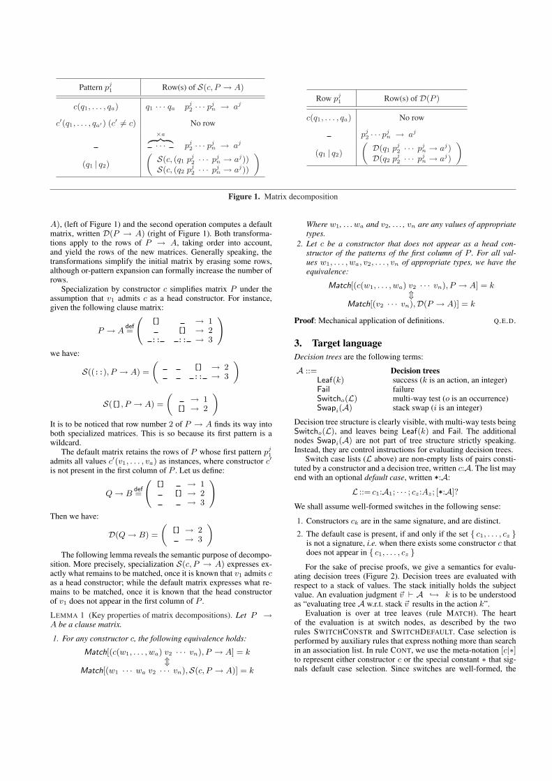
The resulting decision tree is best described as the picture of Fig-ure 3. We now consider examining ys first. That is, we swap the

xs

1

2

3

[]

ys

(::) []

(::)

Figure 3. Compilation of list-merge, left-to-right

2 In examples, initial occurrences are written as names. Formally we candefine xs to be occurrence 1 and ys to be occurrence 2.

two columns of ~o and P , yielding the new arguments:

~o ′ = (ys xs) P ′ → A =

([] → 1

[] → 2:: :: → 3

)

Specialized matrices are as follows:

S(::, P ′ → A) =

([] → 1:: → 3

)

S([], P ′ → A) =

([] → 1→ 2

)

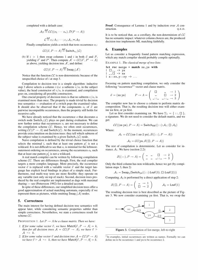
Finally, compilation yields the decision tree of Figure 4. Notice

ys 1

xs[]

xs

(::)

[]

2*

[]

3

(::)

Figure 4. Compilation of list-merge, right-to-left

that the leaf “1” is pictured as shared, thereby reflecting actualimplementation. The pictures clearly suggest that the left-to-rightdecision tree is better than the right-to-left one, in two importantaspects.

1. The first decision tree is smaller. A simple measure of decisiontree size is the number of internal nodes, that is, the number ofswitches.

2. The first decision tree is more efficient: if xs is the emptylist [], then the tree of Figure 3 reaches action 1 by performingone test only, while the tree of Figure 4 always performs twotests.

In this simple case, all decision trees are available and can becompared. A compiler cannot rely on such a post-mortem analysis,which can be extremely expensive. Instead, a compilation heuristicwill select a column in P at every critical step 3, based uponproperties of matrix P . Such properties should be simple, relativelycheap to compute and have a positive impact on the quality of theresulting decision tree.

Before we investigate heuristics any further, let us consider anexample that illustrates the implementation of decision trees bydags with maximal sharing.

EXAMPLE 2. Consider the following matching expression where[_] is OCaml pattern for “a list of one element” (i.e. _::[]):

match xs,ys with [_],_ -> 1 | _,[_] -> 2

Naive compilation of the example yields the decision tree that isdepicted as a dag with maximal sharing in Figure 5. The dag of Fig-

xs

fail

ys

*

ys.2

(::)*

2[]

*

xs.2

(::) *

1[]

Figure 5. Decision tree as a dag with maximal sharing

ure 5 has 2+2 = 4 switch nodes, where a plain tree implementationhas 2 + 2 × 2 = 6 switch nodes. Now consider a simple general-ization: a diagonal pattern matrix, of size n× n with pii =[_] andpji = for i 6= j. It is not difficult to see that the dag representationof the naive decision tree has 2n switch nodes, where the plain treerepresentation has 2n+1 − 2 switch nodes. Or-pattern compilationalso benefits from maximal sharing. Let us consider for instancethe n-tuple pattern (1|2),. . .,(1|2). Compilation produces a treewith 2n − 1 switches and a dag with n switches. One may also re-mark that, for a clause matrix of one row, such that some of itspatterns are or-patterns, maximal sharing makes column choice in-different. While, without maximal sharing, or-patterns should bet-ter be expanded last. As a conclusion, maximal sharing is a simpleidea that may yield important savings in code size.

Finally, here is a more a realistic example.

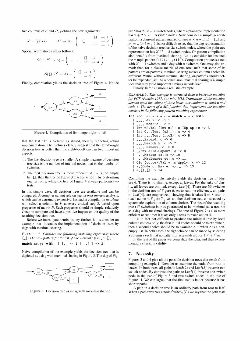
EXAMPLE 3. This example is extracted from a bytecode machinefor PCF (Plotkin 1977) (or mini-ML). Transitions of the machinedepend upon the values of three items: accumulator a, stack s andcode c. The heart of a ML function that implements the machineconsists in the following pattern matching expression:

l e t rec run a s e c = match a,s,c with| _,_,Ldi i::c -> 1| _,_,Push::c -> 2| Int n2,Val (Int n1)::s,IOp op::c -> 3| Int 0,_,Test (c2,_)::c -> 4| Int _,_,Test (_,c3)::c -> 5| _,_,Extend::c -> 6| _,_,Search k::c -> 7| _,_,Pushenv::c -> 8| _,Env e::s,Popenv::c -> 9| _,_,Mkclos cc::c -> 10| _,_,Mkclosrec cc::c -> 11| Clo (cc,ce),Val v::s,Apply::c -> 12| a,(Code c::Env e::s),[] -> 13| a,[],[] -> 14

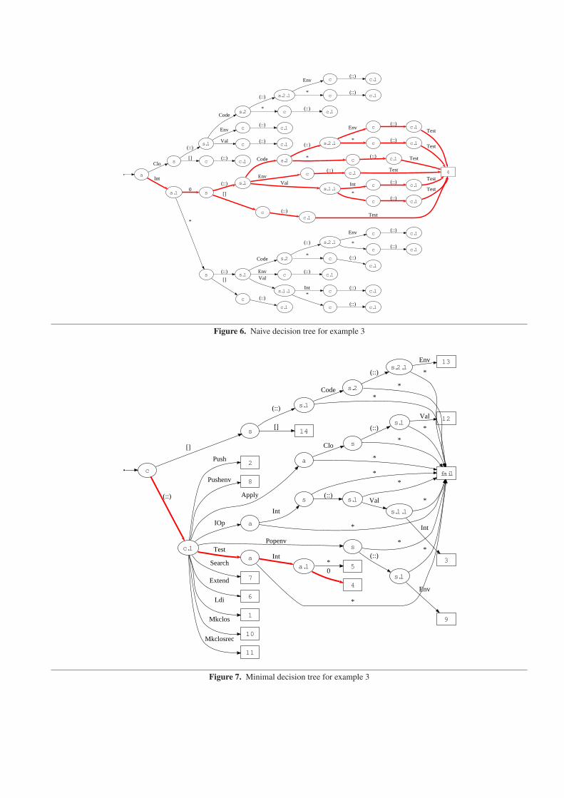
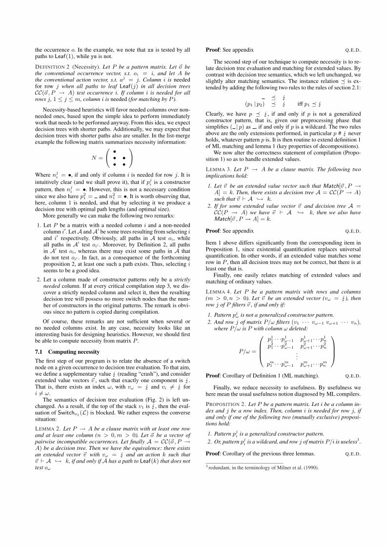
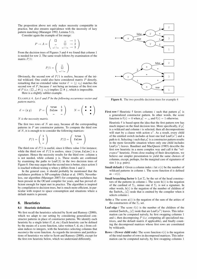
Compiling the example naively yields the decision tree of Fig-ure 6. There is no sharing, except at leaves. For the sake of clar-ity, all leaves are omitted, except Leaf(4). There are 56 switchesin the decision tree of Figure 6. As to runtime efficiency, all pathsto Leaf(4), are emphasized, showing that it takes 5 to 8 tests toreach action 4. Figure 7 gives another decision tree, constructed bysystematic exploration of column choices. The size of the resultingtree (17 switches) is thus guaranteed to be minimal (as a tree notas a dag with maximal sharing). The tree of Figure 7 is also moreefficient at runtime: it takes only 4 tests to reach action 4.

It is in fact not difficult to produce the minimal tree by localcolumn choices only: the first initial choice should be to examine c,then a second choice should be to examine c.1 when c is a non-empty list. In both cases, the right choice can be made by selectinga column i such that no pattern pji is a wildcard for 1 ≤ j ≤ m.

In the rest of the paper we generalize the idea, and then experi-mentally check its validity.

7. NecessityFigures 3 and 4 give all the possible decision trees that result fromcompiling example 1. Now, let us examine the paths from root toleaves. In both trees, all paths to Leaf(2) and Leaf(3) traverse twoswitch nodes. By contrast, the paths to Leaf(1) traverse one switchnode in the tree of Figure 3 and two switch nodes in the tree ofFigure 4. We can argue that the first tree is better because it hasshorter paths.

A path in a decision tree is an ordinary path from root to leaf.When a path traverses a node Switcho(L) we say that the path tests

a4

sClo

a.1

Int

s.1(::)

c[]

s.2Code

cEnv

cVal

s.2.1(::)

c*

cEnv

c*

c.1(::)

c.1(::)

c.1(::)

c.1(::)

c.1(::)

c.1(::)

s0

s

*

s.1(::)

c

[]

s.2Code

cEnv

s.1.1

Val

s.2.1(::)

c*

cEnv

c*

c.1(::)

Test

c.1(::)

Test

c.1(::) Test

c.1(::) Test

cInt

c

*

c.1(::)

Test

c.1(::)

Test

c.1

(::)Test

s.1(::)

c

[]

s.2Code

cEnv

s.1.1

Val

s.2.1(::)

c*

cEnv

c

*

c.1(::)

c.1(::)

c.1

(::)

c.1(::)

cInt

c

*c.1

(::)

c.1(::)

c.1

(::)

Figure 6. Naive decision tree for example 3

cfail

c.1

(::)

s

[]

a

Apply

6

Extend

aIOp

1

Ldi

10

Mkclos

11

Mkclosrec

s

Popenv

2Push

8Pushenv

7

Searcha

Test

*

sClo*

s.1(::) *

12Val

*

s

Int

*

s.1(::)

*

s.1.1

Val *

3

Int

*

s.1

(::)*

9

Env

*

a.1

Int

4

05

*

s.1(::)

14[]

*s.2Code

*

s.2.1(::) *

13Env

Figure 7. Minimal decision tree for example 3

the occurrence o. In the example, we note that xs is tested by allpaths to Leaf(1), while ys is not.

DEFINITION 2 (Necessity). Let P be a pattern matrix. Let ~o bethe conventional occurrence vector, s.t. oi = i, and let A bethe conventional action vector, s.t. aj = j. Column i is neededfor row j when all paths to leaf Leaf(j) in all decision treesCC(~o , P → A) test occurrence i. If column i is needed for allrows j, 1 ≤ j ≤ m, column i is needed (for matching by P ).

Necessity-based heuristics will favor needed columns over non-needed ones, based upon the simple idea to perform immediatelywork that needs to be performed anyway. From this idea, we expectdecision trees with shorter paths. Additionally, we may expect thatdecision trees with shorter paths also are smaller. In the list-mergeexample the following matrix summarizes necessity information:

N =

( •• •• •

)

Where nji = •, if and only if column i is needed for row j. It isintuitively clear (and we shall prove it), that if pji is a constructorpattern, then nji = •. However, this is not a necessary conditionsince we also have p2

1 = and n21 = •. It is worth observing that,

here, column 1 is needed, and that by selecting it we produce adecision tree with optimal path lengths (and optimal size).

More generally we can make the following two remarks:

1. Let P be a matrix with a needed column i and a non-neededcolumn i′. LetA andA′ be some trees resulting from selecting iand i′ respectively. Obviously, all paths in A test oi, whileall paths in A′ test oi′ . Moreover, by Definition 2, all pathsin A′ test oi, whereas there may exist some paths in A thatdo not test oi′ . In fact, as a consequence of the forthcomingproposition 2, at least one such a path exists. Thus, selecting iseems to be a good idea.

2. Let a column made of constructor patterns only be a strictlyneeded column. If at every critical compilation step 3, we dis-cover a strictly needed column and select it, then the resultingdecision tree will possess no more switch nodes than the num-ber of constructors in the original patterns. The remark is obvi-ous since no pattern is copied during compilation.

Of course, these remarks are not sufficient when several orno needed columns exist. In any case, necessity looks like aninteresting basis for designing heuristics. However, we should firstbe able to compute necessity from matrix P .

7.1 Computing necessityThe first step of our program is to relate the absence of a switchnode on a given occurrence to decision tree evaluation. To that aim,we define a supplementary value (reading “crash”), and considerextended value vectors ~v , such that exactly one component is .That is, there exists an index ω, with vω = and vi 6= fori 6= ω.

The semantics of decision tree evaluation (Fig. 2) is left un-changed. As a result, if the top of the stack v1 is , then the eval-uation of Switcho1(L) is blocked. We rather express the conversesituation:

LEMMA 2. Let P → A be a clause matrix with at least one rowand at least one column (n > 0,m > 0). Let ~o be a vector ofpairwise incompatible occurrences. Let finally A = CC(~o , P →A) be a decision tree. Then we have the equivalence: there existsan extended vector ~v with vω = and an action k such that~v ` A ↪→ k, if and only ifA has a path to Leaf(k) that does nottest oω

Proof: See appendix Q.E.D.

The second step of our technique to compute necessity is to re-late decision tree evaluation and matching for extended values. Bycontrast with decision tree semantics, which we left unchanged, weslightly alter matching semantics. The instance relation ¹ is ex-tended by adding the following two rules to the rules of section 2.1:

¹ (p1 | p2) ¹ iff p1 ¹

Clearly, we have p ¹ , if and only if p is not a generalizedconstructor pattern, that is, given our preprocessing phase thatsimplifies ( | p) as , if and only if p is a wildcard. The two rulesabove are the only extensions performed, in particular p # neverholds, whatever pattern p is. It is then routine to extend definition 1of ML matching and lemma 1 (key properties of decompositions).

We now alter the correctness statement of compilation (Propo-sition 1) so as to handle extended values.

LEMMA 3. Let P → A be a clause matrix. The following twoimplications hold:

1. Let ~v be an extended value vector such that Match[~v , P →A] = k. Then, there exists a decision tree A = CC(P → A)such that ~v ` A ↪→ k.

2. If for some extended value vector ~v and decision tree A =CC(P → A) we have ~v ` A ↪→ k, then we also haveMatch[~v , P → A] = k.

Proof: See appendix Q.E.D.

Item 1 above differs significantly from the corresponding item inProposition 1, since existential quantification replaces universalquantification. In other words, if an extended value matches somerow in P , then all decision trees may not be correct, but there is atleast one that is.

Finally, one easily relates matching of extended values andmatching of ordinary values.

LEMMA 4. Let P be a pattern matrix with rows and columns(m > 0, n > 0). Let ~v be an extended vector (vω = ), thenrow j of P filters ~v , if and only if:

1. Pattern pjω is not a generalized constructor pattern.2. And row j of matrix P/ω filters (v1 · · · vω−1 vω+1 · · · vn),

where P/ω is P with column ω deleted:

P/ω =

p11 · · ·p1

ω−1 p1ω+1· · ·p1

n

p21 · · ·p2

ω−1 p2ω+1· · ·p2

n

...pm1 · · ·pmω−1 pmω+1· · ·pmn

Proof: Corollary of Definition 1 (ML matching). Q.E.D.

Finally, we reduce necessity to usefulness. By usefulness wehere mean the usual usefulness notion diagnosed by ML compilers.

PROPOSITION 2. Let P be a pattern matrix. Let i be a column in-dex and j be a row index. Then, column i is needed for row j, ifand only if one of the following two (mutually exclusive) proposi-tions hold:

1. Pattern pji is a generalized constructor pattern.2. Or, pattern pji is a wildcard, and row j of matrix P/i is useless3.

Proof: Corollary of the previous three lemmas. Q.E.D.

3 redundant, in the terminology of Milner et al. (1990).

The proposition above not only makes necessity computable inpractice, but also ensures equivalence with the necessity of lazypattern matching (Maranget 1992, Lemma 5.1).

Consider again the example of list merge:

P → A =

([] → 1

[] → 2:: :: → 3

)

From the decision trees of Figures 3 and 4 we found that column 1is needed for row 2. The same result follows by examination of thematrix P/1:

P/1 =

([]::

)

Obviously, the second row of P/1 is useless, because of the ini-tial wildcard. One could also have considered matrix P directly,remarking that no extended value vector ~v = ( v2) matches thesecond row of P , because ~v not being an instance of the first rowof P (i.e. ([] ) # ( v2)) implies [] # , which is impossible.

Here is a slightly subtler example.

EXAMPLE 4. Let ~o and P be the following occurrence vector andpattern matrix.

~o = (x y) P =

(true 1false 2

)N =

( • •• ••

)

N is the necessity matrix.

The first two rows of N are easy, because all the correspondingpatterns in P are constructor patterns. To compute the third rowof N , it is enough to to consider the following matrices:

P/1 =

(12

)P/2 =

(truefalse

)

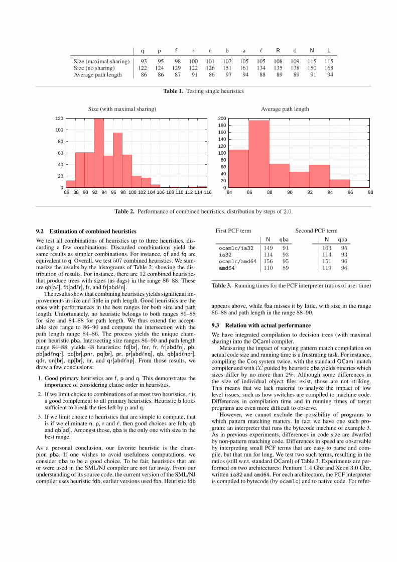
The third row of P/1 is useful, since it filters value 3 for instance;while the third row of P/2 is useless, since { true, false } is asignature. Hence the necessity results for the third row: column xis not needed, while column y is. These results are confirmedby examining the paths to Leaf(3) in the two decision trees ofFigure 8. One may argue that the second tree is better, since action 3is reached without testing x when y differs from 1 and 2.

In the general case, it should probably be mentioned that theusefulness problem is NP-complete (Sekar et al. 1995). Neverthe-less, our algorithm (Maranget 2007) for computing usefulness hasbeen present in the OCaml compiler for years, and has proved ef-ficient enough for input met in practice. The algorithm is inspiredby compilation to decision trees, but is much more efficient, in par-ticular with respect to space consumption and situations where adefault matrix is present.

8. Heuristics8.1 Heuristic definitionsWe first recall the heuristics selected by Scott and Ramsey (2000),which we adapt to our setting by considering generalized con-structor patterns in place of constructor patterns. We identify eachheuristic by a single letter (f, d, etc.) Each heuristic can be definedby the means of a score function, (also written f, d, etc.) from col-umn indices to integers, with the heuristics selecting columns thatmaximize the score function. As regards the inventors and justifica-tions of heuristics we refer to Scott and Ramsey (2000), except forthe first row heuristic below, which we understand differently.

x 3

yfalse

y

true

*

22

*

1

1

y 3*

x

2

x

1

*

2false

*

1true

Figure 8. The two possible decision trees for example 4

First row f Heuristic f favors columns i such that pattern p1i is

a generalized constructor pattern. In other words, the scorefunction is f(i) = 0 when p1

i = , and f(i) = 1 otherwise.Heuristic f is based upon the idea that the first pattern row hasmuch impact on the final decision tree. More specifically, if p1

i

is a wildcard and column i is selected, then all decompositionswill start by a clause with action a1. As a result, every childof the emitted switch includes at least one leaf Leaf(a1) and apath to it. Selecting i such that p1

i is a constructor pattern resultsin the more favorable situation where only one child includesLeaf(a1) leaves. Baudinet and MacQueen (1985) describe thefirst row heuristic in a more complex way and call it the “rel-evance” heuristic. From close reading of their descriptions, webelieve our simpler presentation to yield the same choices ofcolumns, except, perhaps, for the marginal case of signatures ofsize 1 (e.g. pairs).

Small default d Given a column index i let v(i) be the number ofwildcard patterns in column i. The score function d is definedas −v(i).

Small branching factor b Let Σi be the set of the head construc-tors of the patterns in column i. The score b(i) is the negationof the cardinal of Σi, minus one if Σi is not a signature. Inother words, b(i) is the negation of the number of children ofthe Switchoi(L) node that is emitted by the compiler when itselects column i.

Arity a The score a(i) is the negation of the sum of the arities ofthe constructors of the Σi set.

Leaf edge ` The score `(i) is the number of the children of theemitted Switchoi(L) node that are Leaf(ak) leaves. This infor-mation can be computed naively, by first swapping columns 1and i, then decomposing P (i.e. computing all specialized ma-trices, and the default matrix if applicable), and finally count-ing the decomposed matrices whose first rows are constitutedby wildcards.

Rows r (Fewer child rule) The score function r(i) is the negationof the total number of rows in decomposed matrices. This infor-mation can be computed naively, by first swapping columns 1

and i, then decomposing P , and finally counting the numbersof rows of the resulting matrices.

We introduce three new heuristics based upon necessity.

Needed columns n The score n(i) is the number of rows j suchthat column i is needed for row j. The intention is quite clear:locally maximize the number of tests that are really useful.

Needed prefix p The score p(i) is the larger row index j such thatcolumn i is needed for all the rows j′, 1 ≤ j′ ≤ j. As theprevious one, this heuristics tends to favor needed columns.However, it further considers that earlier clauses (i.e. the oneswith higher priorities) have more impact on decision tree sizeand path lengths than later ones.

Constructor prefix q This heuristic derives from the previous one,approximating “column i is needed for row j” by “pji is ageneralized constructor pattern”. There are two ideas here: (1)avoid usefulness computations; and (2), avoid pattern copies.Namely, if column i is selected, then any row j such that pji isa wildcard is copied. As a consequence, the other patterns inrow j may be compiled more than once, regardless of whethercolumn i is needed or not. Heuristic q can also be seen as ageneralization of heuristic f.Observe that heuristic d is a similar approximation of heuristic n.

It should be noticed that if matrix P has needed columns, thenheuristics n and p will select these and only these. Similarly, ifmatrix P has strictly needed columns, then heuristics d and q willselect these and only these. Heuristics n and p will also favorstrictly needed columns but they will not distinguish them fromother needed columns.

8.2 Combining heuristicsBy design, heuristics select at least one column. However, a givenheuristic may select several columns. Ties are broken first by com-posing heuristics. For instance, Baudinet and MacQueen (1985)seem to recommend the successive application of f, b and a, whichwe write fba. For instance, consider a variation on example 4.

P =

(true 1false 2 []

::

)

Heuristic f selects columns 1 and 2. Amongst those, heuristic bselects column 1. Column selection being over, there is no needto apply heuristic a. The combination of heuristics is a simpletechnique to construct sophisticated heuristics out of simple ones.It should be noticed that combination order matters, since an earlyheuristic may eliminate columns that a following heuristics wouldchampion.

Even when combined, heuristics may not succeed in selectinga unique column — consider a matrix with identical columns. Wethus define the following three, last-resort, pseudo-heuristics:

Pseudo-heuristics N, L and R These select one column i amongstmany, by selecting the minimal oi in vector ~o according to var-ious total orderings on occurrences. Heuristic N uses the left-most ordering (this is naive compilation). Heuristics L and Rfirst select shorter occurrences, and then break ties left-to-rightor right-to-left, respectively. In other words, L and R are twovariations on breadth-first ordering of the subterms of the sub-ject value.

We call N, L and R pseudo-heuristics, because they do not examinematrix P and thus more rely on accidental presentation of match-ings than on semantics. Varying the last-resort heuristic permits amore accurate evaluation of heuristics.

9. Performance9.1 MethodologyWe have written a prototype compiler that accepts pattern matricesand compiles them with various match compilers The implementedmatch compiler includes compilation to decision trees, both withand without maximal sharing and the optimizing compiler of LeFessant and Maranget (2001), which is the standard OCaml matchcompiler. The prototype compiler targets matching automata, ex-pressed as a simplified version of the first intermediate language ofthe OCaml compiler (Leroy et al. 2007). This target language fea-tures local bindings, indexed memory reads, switches, and localfunctions. Local functions implement maximal sharing or back-tracking, depending upon the compilation algorithm enabled. Weused the prototype to produce all the pictures in this paper, switchnodes being pictured as internal nodes, variables binding memoryread expressions being used to decorate switch nodes, and localfunction definitions being rendered as nodes with several ingoingedges.

The performance of matching automata is estimated as follows:

1. Code size is estimated as the total number of switches.

2. Runtime performance is estimated as average path length. Ide-ally, average path length should be computed with respect tosome distribution of subject values that is independent of theautomaton considered. In practice, we compute average pathlength by assuming that: (1) all actions are equally likely4

and (2), all constructors that can be found by a switch areequally likely5.

To feed the prototype, we have extracted pattern matching ex-pressions from a variety of OCaml programs, including the OCamlcompiler itself, the Coq (Coq) and Why (Filliatre 2008) proof as-sistants, and the Cil infrastructure for C program analysis (Neculaet al. 2007). The selected matchings were identified by a modifiedOCaml compiler that performs match compilation by several algo-rithms and signals differences in number of switch generated —more specifically we used the standard OCaml match compiler andnaive CC without sharing.

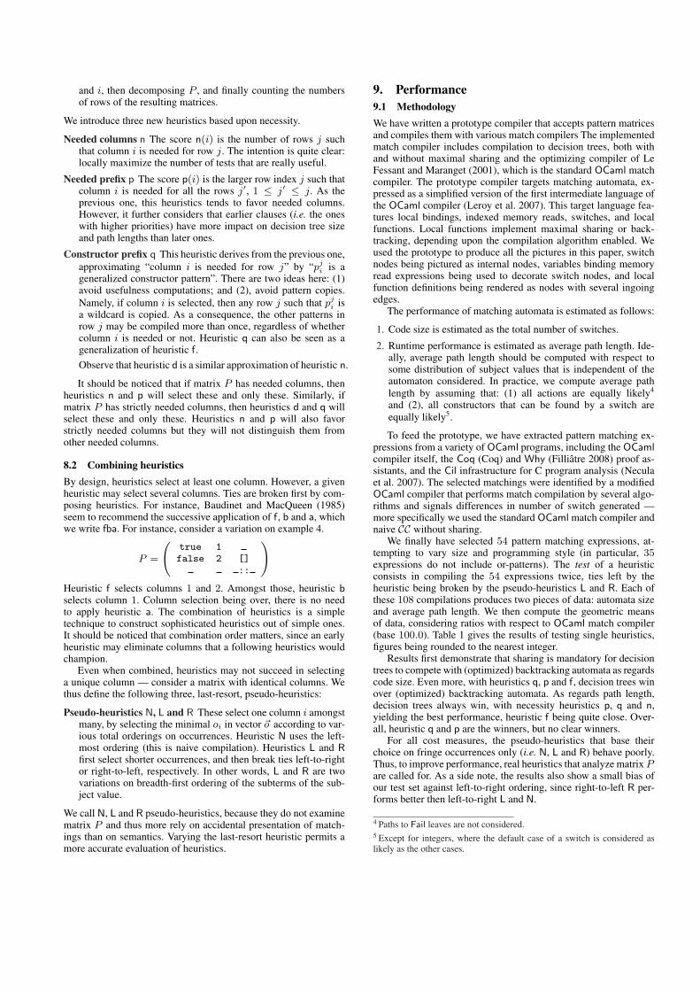
We finally have selected 54 pattern matching expressions, at-tempting to vary size and programming style (in particular, 35expressions do not include or-patterns). The test of a heuristicconsists in compiling the 54 expressions twice, ties left by theheuristic being broken by the pseudo-heuristics L and R. Each ofthese 108 compilations produces two pieces of data: automata sizeand average path length. We then compute the geometric meansof data, considering ratios with respect to OCaml match compiler(base 100.0). Table 1 gives the results of testing single heuristics,figures being rounded to the nearest integer.

Results first demonstrate that sharing is mandatory for decisiontrees to compete with (optimized) backtracking automata as regardscode size. Even more, with heuristics q, p and f, decision trees winover (optimized) backtracking automata. As regards path length,decision trees always win, with necessity heuristics p, q and n,yielding the best performance, heuristic f being quite close. Over-all, heuristic q and p are the winners, but no clear winners.

For all cost measures, the pseudo-heuristics that base theirchoice on fringe occurrences only (i.e. N, L and R) behave poorly.Thus, to improve performance, real heuristics that analyze matrix Pare called for. As a side note, the results also show a small bias ofour test set against left-to-right ordering, since right-to-left R per-forms better then left-to-right L and N.

4 Paths to Fail leaves are not considered.5 Except for integers, where the default case of a switch is considered aslikely as the other cases.

q p f r n b a ` R d N L

Size (maximal sharing) 93 95 98 100 101 102 105 105 108 109 115 115Size (no sharing) 122 124 129 122 126 151 161 134 135 138 150 168Average path length 86 86 87 91 86 97 94 88 89 89 91 94

Table 1. Testing single heuristics

Size (with maximal sharing)

0

20

40

60

80

100

120

86 88 90 92 94 96 98 100 102 104 106 108 110 112 114 116

Average path length

0

20

40

60

80

100

120

140

160

180

200

84 86 88 90 92 94 96 98

Table 2. Performance of combined heuristics, distribution by steps of 2.0.

9.2 Estimation of combined heuristicsWe test all combinations of heuristics up to three heuristics, dis-carding a few combinations. Discarded combinations yield thesame results as simpler combinations. For instance, qf and fq areequivalent to q. Overall, we test 507 combined heuristics. We sum-marize the results by the histograms of Table 2, showing the dis-tribution of results. For instance, there are 12 combined heuristicsthat produce trees with sizes (as dags) in the range 86–88. Theseare qb[a`], fb[ad`r], fr, and fr[abd`n].

The results show that combining heuristics yields significant im-provements in size and little in path length. Good heuristics are theones with performances in the best ranges for both size and pathlength. Unfortunately, no heuristic belongs to both ranges 86–88for size and 84–88 for path length. We thus extend the accept-able size range to 86–90 and compute the intersection with thepath length range 84–86. The process yields the unique cham-pion heuristic pba. Intersecting size ranges 86–90 and path lengthrange 84–88, yields 48 heuristics: fd[br], fnr, fr, fr[abd`n], pb,pb[ad`nqr], pd[br],pnr, pq[br], pr, pr[abd`nq], qb, qb[ad`npr],qdr, qn[br], qp[br], qr, and qr[abd`np]. From those results, wedraw a few conclusions:

1. Good primary heuristics are f, p and q. This demonstrates theimportance of considering clause order in heuristics.

2. If we limit choice to combinations of at most two heuristics, r isa good complement to all primary heuristics. Heuristic b lookssufficient to break the ties left by p and q.

3. If we limit choice to heuristics that are simple to compute, thatis if we eliminate n, p, r and `, then good choices are fdb, qband qb[ad]. Amongst those, qba is the only one with size in thebest range.

As a personal conclusion, our favorite heuristic is the cham-pion pba. If one wishes to avoid usefulness computations, weconsider qba to be a good choice. To be fair, heuristics that areor were used in the SML/NJ compiler are not far away. From ourunderstanding of its source code, the current version of the SML/NJcompiler uses heuristic fdb, earlier versions used fba. Heuristic fdb

First PCF termN qba

ocamlc/ia32 149 91ia32 114 93ocamlc/amd64 156 95amd64 110 89

Second PCF termN qba

163 95114 93151 96119 96

Table 3. Running times for the PCF interpreter (ratios of user time)

appears above, while fba misses it by little, with size in the range86–88 and path length in the range 88–90.

9.3 Relation with actual performanceWe have integrated compilation to decision trees (with maximalsharing) into the OCaml compiler.

Measuring the impact of varying pattern match compilation onactual code size and running time is a frustrating task. For instance,compiling the Coq system twice, with the standard OCaml matchcompiler and with CC guided by heuristic qba yields binaries whichsizes differ by no more than 2%. Although some differences inthe size of individual object files exist, those are not striking.This means that we lack material to analyze the impact of lowlevel issues, such as how switches are compiled to machine code.Differences in compilation time and in running times of targetprograms are even more difficult to observe.

However, we cannot exclude the possibility of programs towhich pattern matching matters. In fact we have one such pro-gram: an interpreter that runs the bytecode machine of example 3.As in previous experiments, differences in code size are dwarfedby non-pattern matching code. Differences in speed are observableby interpreting small PCF terms that are easy to parse and com-pile, but that run for long. We test two such terms, resulting in theratios (still w.r.t. standard OCaml) of Table 3. Experiments are per-formed on two architectures: Pentium 1.4 Ghz and Xeon 3.0 Ghz,written ia32 and amd64. For each architecture, the PCF interpreteris compiled to bytecode (by ocamlc) and to native code. For refer-

ence, average path length are 4.02 for the OCaml match compiler,6.33 for N, and 3.14 for qba (ratios: 157 for N and 78 for qba).We see that differences in speed agree with differences in averagepath length. Moreover, running times are indeed bad if heuristicsare neglected, especially for compilation to bytecode.

10. Related workMaximal sharing can be achieved by the easy to implement andwell established technique of hash-consing — see e.g. Filliatre andConchon (2006). With hash-consing, the asymptotic cost of pro-ducing the dag is about the same as the one of the tree. Some (Sekaret al. 1995; Nedjah and de Macedo Mourelle 2002) advocate an-other technique that do not suffer from this drawback. More pre-cisely, they compute some key from the match compiler arguments,such that key identity implies tree identity. Such keys are also use-ful for establishing upper bounds on the size of the dag. In practice,hash-consing seems to be sufficient, both for the prototype and forthe modified OCaml compiler.

Needed columns exactly are the directions of Laville (1988);Puel and Suarez (1989); Maranget (1992). All these authors buildover lazy pattern semantics, adapting the seminal work of Huet andLevy (1991). They mostly focus on the correct implementation oflazy pattern matching. By building over decision tree semantics,our present work leads more directly to heuristic design. Sekaret al. (1995) claim to have proved that selecting one of their indices(our needed columns) yields trees with shorter path lengths andsmaller breadth (number of leaves in plain tree representation).Their results need a careful formulation in the general case, but areintuitively clear on example 4. The result on tree breadth is wrong,as demonstrated by the trees of Figure 8. The second decision treeis built by selecting needed columns and has breadth 5 (count edgesto leaves), whereas the breadth of the first tree is 4. We conjecturethe result on path lengths to be significant.

Scott and Ramsey (2000) study heuristics experimentally. Weimprove on them by designing and testing the necessity-basedheuristics, and also by considering or-patterns and maximal shar-ing. We also differ in methodology: Scott and Ramsey (2000) countswitch nodes and measure path lengths, as we do, but they do so forcomplete ML programs by instrumenting the SML/NJ compiler. Asa result, their experiments are more expensive than ours, and theycould not conduct systematic experiments on combination of threeheuristics. Furthermore, by our prototype approach, we restrict thetest set to matchings for which heuristics make a difference. There-fore, differences in measures are more striking. Of course, as re-gards actual compilation, we are in the same situation as Scott andRamsey (2000): most often, heuristics do not make such a differ-ence. However, heuristics matter to some of the tests of Scott andRamsey (2000) (machine instruction recognizers). It would be par-ticularly interesting to test the effect of necessity heuristics and ofmaximal sharing on those matchings, which, unfortunately, are notavailable.

11. ConclusionCompilation to decision trees with maximal sharing, when guidedby a good column heuristic, matches the performance of an op-timizing compiler to backtracking automata, and can do better onsome examples. Moreover, an optimizing compiler to decision treesis easier to implement than our own optimizing compiler to back-tracking automata (Le Fessant and Maranget 2001). Namely, max-imal sharing and simple heuristics (such as qba) are orthogonalextensions of the basic compilation scheme CC. Thus, the resultingoptimizing match compiler remains simple.

Designing optimizing match compilers that preserve more con-strained semantics is a worthwhile direction for future research. In

particular, a match compiler for Haskell must preserve the termina-tion behavior of Augustsson (1985). Another example is the com-pilation of the active patterns of Syme et al. (2007). To that aim,the match compiler of Sestoft (1996) may be a valid starting point,because its definition follows ML matching semantics very closely.

ReferencesLennart Augustsson. Compiling pattern matching. In Conference on

Functional Programming Languages and Computer Architecture, 1985.Marianne Baudinet and David B. MacQueen. Tree pattern match-

ing for ML. http://www.smlnj.org/compiler-notes/85-note-baudinet.ps, 1985.

Coq. The Coq proof assistant (v. 8.1). By the Coq team, http://coq.inria.fr/, 2007.

Jean-Christophe Filliatre. The Why verification tool (v. 2.13). http://why.lri.fr/, 2008.

Jean-Christophe Filliatre and Sylvain Conchon. Type-safe modular hash-consing. In Workshop on ML. ACM Press, 2006.

Gerard Huet and Jean-Jacques Levy. Call by need computations in non-ambiguous linear term rewriting systems. In Jean-Louis Lassez andGordon D. Plotkin, editors, Computational Logic, Essays in Honor ofAlan Robinson. The MIT Press, 1991.

Alain Laville. Implementation of lazy pattern matching algorithms. In Eu-ropean Symposium on Programming. Springer-Verlag, 1988. LNCS 300.

Fabrice Le Fessant and Luc Maranget. Optimizing pattern matching. In In-ternational Conference on Functional Programming. ACM Press, 2001.

Xavier Leroy, Damien Doligez, Jacques Garrigue, Jerome Vouillon, andDidier Remy. The Objective Caml language (v. 3.10). http://caml.inria.fr, 2007.

Luc Maranget. Warnings for pattern matching. Journal of FunctionalProgramming, 17:387–422, May 2007.

Luc Maranget. Compiling lazy pattern matching. In Conference on Lispand Functional Programming, 1992.

Robin Milner, Mads Tofte, and Robert Harper. The Definition of StandardML. MIT Press, Cambridge, MA, 1990.

George Necula, Scott McPeak, Westley Weimer, Ben Liblit, Matt Harren,Ramond To, and Aman Bhargava. Cil — infrastructure for C programanalysis and transformation (v. 1.3.6). http://manju.cs.berkeley.edu/cil/, 2007.

Nadia Nedjah and Luiza de Macedo Mourelle. Optimal adaptive patternmatching. In Developments in Applied Artificial Intelligence, 2002.LNCS 2358.

Scott Owens. A sound semantics for OCaml-Light. In European Sympho-sium On Programming, 2008. LNCS 4960.

Mikael Pettersson. A term pattern-match compiler inspired by finite au-tomata theory. In Workshop on Compiler Construction. Springer-Verlag,1992. LNCS 641.

Gordon D. Plotkin. LCF considered as a programming language. Theoreti-cal Computer Science, 5:225–255, December 1977.

Laurence Puel and Ascander Suarez. Compiling pattern matching by termdecomposition. In Conference on LISP and Functional Programming.ACM Press, 1989.

Kevin Scott and Norman Ramsey. When do match-compilation heuristicsmatter? Technical Report CS-2000-13, University of Virginia, 2000.

R.C. Sekar, R. Ramesh, and I. V. Ramakrishnan. Adaptive pattern matching.SIAM Journal on Computing, 24:1207–1243, December 1995.

Peter Sestoft. ML pattern matching compilation and partial evaluation.In Dagstuhl Seminar on Partial Evaluation. Springer-Verlag, 1996.LNCS 1110.

Son Syme, Gregory Neverov, and James Margetson. Extensible patternmatching via a lighweight language extension. In International Confer-ences on Functional Programming. ACM Press, 2007.

Terese. Term Rewriting Systems. Cambridge University Press, 2003. Tereseis Marc Bezem, Jan Willem Klop and Roel de Vrier.

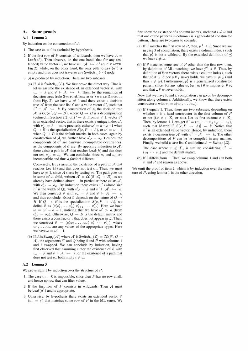
A. Some proofsA.1 Lemma 2By induction on the construction of A.

1. The case m = 0 is excluded by hypothesis.

2. If the first row of P consists of wildcards, then we have A =Leaf(a1). Then observe, on the one hand, that for any (ex-tended) value vector ~v , we have ~v ` A ↪→ a1 (rule MATCH,Fig 2); while, on the other hand, the only path to Leaf(a1) isempty and thus does not traverse any Switchoω (· · ·) node.

3. A is produced by induction. There are two subcases.

(a) If A is Switcho1(L). We first prove the direct way. That is,let us assume the existence of an extended vector ~v , withvω = and ~v ` A ↪→ k. Then, by the semantics ofdecision trees (rule SWITCHCONSTR or SWITCHDEFAULTfrom Fig. 2), we have ω 6= 1 and there exists a decisiontree A′ from the case list L and a value vector ~v ′, such that~v ′ ` A′ ↪→ k. By construction of A, the decision treeA′ is CC(~o ′, Q → B), where Q → B is a decomposition(defined in Section 2.2) of P → A. From ω 6= 1, vector ~v ′

is an extended vector, that is there exists a unique index ω′,with v′ω′ = — more precisely, either ω′ = a+ω−1 whenQ→ B is the specialization S(c, P → A), or ω′ = ω − 1when Q → B is the default matrix. In both cases, again byconstruction of A, we further have o′ω′ = oω . Besides, thecomponents of ~o ′ are pairwise incompatible occurrences,as the components of ~o are. By applying induction to A′,there exists a path in A′ that reaches Leaf(k) and that doesnot test o′ω′ = oω . We can conclude, since o1 and oω areincompatible and thus a fortiori different.Conversely, let us assume the existence of a path in A thatreaches Leaf(k) and that does not test oω . Then, we musthave ω 6= 1, since A starts by testing o1. The path goes onin some of A child, written A′ = CC(~o ′, Q → B), as wealready have defined above — in particular there exists ω′,with o′ω′ = oω . By induction there exists ~v ′ (whose sizen′ is the width of Q), with v′ω′ = and ~v ′ ` A′ ↪→ k.We then construct ~v with vω = and ~v ` A ↪→ kand thus conclude. Exact ~v depends on the nature of Q →B. If Q → B is the specialization S(c, P → A), wedefine ~v as (c(v′1, . . . , v

′a) v′a+1 · · · v′n′). Here we have

ω = ω′ − a + 1, noticing that we have ω′ > a (fromo′ω′ = oω). Otherwise, Q → B is the default matrix andthere exists a constructor c that does not appear in L. Then,we construct ~v = (c(w1, . . . , wa) v′1 · · · v′n′), wherew1, . . . , wa are any values of the appropriate types. Herewe have ω = ω′ + 1.

(b) IfA is Swapi(A′) whereA′ is Switchoi(L) = CC(~o ′, Q→A), the arguments ~o ′ and Q being ~o and P with columns 1and i swapped. We can conclude by induction, havingfirst observed that assuming either the existence of ~v withvω = and ~v ` A ↪→ k, or the existence of a path thatdoes not test oω both imply i 6= ω.

A.2 Lemma 3We prove item 1 by induction over the structure of P .

1. The case m = 0 is impossible, since then P has no row at all,and hence no row that can filter values.

2. If the first row of P consists in wildcards. Then A mustbe Leaf(a1) and is appropriate.

3. Otherwise, by hypothesis there exists an extended vector ~v(vω = ) that matches some row of P in the ML sense. We

first show the existence of a column index i, such that i 6= ω andthat one of the patterns in column i is a generalized constructorpattern. There are two cases to consider.

(a) If ~v matches the first row of P , then, ~p 1 ¹ ~v . Since we arein case 3 of compilation, there exists a column index i suchthat p1

i is not a wildcard. By the extended definition of ¹we have i 6= ω.

(b) If ~v matches some row of P other than the first row, then,by definition of ML matching, we have ~p 1 # ~v . Thus, bydefinition of # on vectors, there exists a column index i, suchthat p1

i # vi. Since p # never holds, we have vi 6= (andthus i 6= ω). Furthermore, p1

i is a generalized constructorpattern, since , for any valuew, (q1 | q2) # w implies q1 # v;and that # w never holds.

Now that we have found i, compilation can go on by decompo-sition along column i. Additionally, we know that there existsconstructor c with v1 = c(w1, . . . , wa).

(a) If i equals 1. Then, there are two subcases, depending onwhether c is a head constructor in the first column of Por not (i.e. c ∈ Σ1 or not). Let us first assume c ∈ Σ1

Then, by lemma 1-1, we get ~v ′ = (w1 · · · wa v2 · · · vn),such that Match[~v ′,S(c, P → A)] = k. Notice that~v ′ is an extended value vector. Hence, by induction, thereexists a decision tree A′ with ~v ′ ` A′ ↪→ k. The otherdecompositions of P can be be compiled in any manner.Finally, we build a case list L and define A = Switch(L).The case where c 6∈ Σ1 is similar, considering ~v ′ =(v2 · · · vn) and the default matrix.

(b) If i differs from 1. Then, we swap columns 1 and i in both~v and P and reason as above.

We omit the proof of item 2, which is by induction over the struc-ture of P , using lemma 1 in the other direction.