Complete Construction of Simple RSM · This is an example of the syntax used to describe the necessary elements of the mesh block. In each ... RSM Training HESM Instructional Materials

RSM Training HESM Instructional Materials for Training Purposes Only Module 4: Editing the RSM

Hydrologic and Environmental Systems Modeling Page 4.1

Lecture 4: Editing the RSM

This lecture reviews the components of a complete RSM. Several features will be discussed in detail in

subsequent lectures.

Complete Construction of Simple RSM Complete Construction of Simple RSM


Page 4.2 Hydrologic and Environmental Systems Modeling

NOTE:

Additional Resources

The HSE User Manual can be found in the labs/lab4_complete_RSM directory.

The AFSIRS documentation can be found in the labs/lab11_hpm directory: Smajstrla, A.G. (1990). Agricultural Field Scale Irrigation Requirements Simulation (AFSIRS) Model. Technical Manual Version 5.5. Agricultural Engineering Dept., University of Florida.



The construction of a complete RSM model will lead to the development of the complete XML run

file, or set of XML files.

1. Construct the appropriate mesh and network. In the previous lecture we discussed the development of the appropriate mesh and network based on the characteristics of your model domain and model objectives. These decisions include the choice of whether to include all canals or only the primary canals.

2. Select the structures that you want included in the model. These include all water flow structures. They can be simulated as watermovers or imposed as boundary conditions. Wells are imposed as stresses on the aquifer using an input flow time series. Structure flow may be simulated or imposed. An important process in hydrologic simulation model implementation in south Florida is the process of calibrating the canal/aquifer and stream bank interaction terms because of the high degree of interaction of the canal with the aquifer. As such, the historical structure flows have been imposed on the canal junctions (flows at the downstream segment and heads on the upstream segment). These models have used the Parameter Estimation program (PEST) to calibrate the model. Calibration will be covered in lectures 13 and 14.

3. Select the other important features that affect the regional hydrology. These may include local hydrology, levees and Water Control Districts. There is a standard set of HPMs that is currently being used with small variations in the individual subregional models (refer to the model files located in $RSM/data/[model], where [model] is one of: C111, Biscayne Bay Coastal Wetlands (BBCW), Glades_LECSA. The levees are modeled using the <leveeSeepage> watermover function. Water Control Districts are special features that are implemented through a set of specific elements.

2

Creating an RSM ImplementationCreating an RSM Implementation

Model Conceptualization

• Conceptualize Mesh and Network

Discretization and framework

Primary and secondary canals to be included

• Determine critical structures

PWS wells

Modeled structures and imposed structures

• Important processes

Local hydrology (HPMs)

Levees/canal seepage

Water Control Districts

Model Conceptualization

• Conceptualize Mesh and Network

Discretization and framework

Primary and secondary canals to be included

• Determine critical structures

PWS wells

Modeled structures and imposed structures

• Important processes

Local hydrology (HPMs)

Levees/canal seepage

Water Control Districts



Input data for parameter values, and time

series data for boundary conditions, are

required to create a complete RSM

implementation.

Although an RSM can be created with only

a mesh or only a network for checking

model connectivity, the minimum model

structural information should include the

2D mesh and the canal network. The control

block provides the model control functions

and the output block defines the output

from the model.

The Header determines which version of the

XML software we are using and the location

of the hse.dtd that is used to parse the input

files.

The Entity element provides the option for

including other XML files. This is useful

when the model input becomes very long

and can be broken into pieces for ease of

viewing and editing.

The Control Section specifies the start and

end times for the simulation, the timestep,

units and the control parameters for PETSc

solver.

The details of the control block are found in

Chapter 2 and Section 3.1 of the HSE User

Manual.

3

Create a simple RSM Create a simple RSM

Input Data

Geographic data (geodatabase)

Time series data (boundary conditions)

RSM components

Control

Mesh

Network

Outputs

Monitors

budgets

Input Data

Geographic data (geodatabase)

Time series data (boundary conditions)

RSM components

Control

Mesh

Network

Outputs Monitors

budgets

4

<control> Block<control> Block



A complete RSM model can have several blocks of XML input code. The yellow highlighted blocks

are the essential components of an RSM‐HSE implementation. Other commonly used waterbodies are

highlighted in orange. If the Management Simulation Engine (MSE) is implemented, than several

additional blocks of code will be necessary. Some blocks such as <streambanks> are no longer used.

5

XML BlocksXML Blocks

entity

control

mesh

network

lakes

basins

wcdwaterbodies

watermovers

rulecurves

impoundments

entity

control

mesh

network

lakes

basins

wcdwaterbodies

watermovers

rulecurves

impoundments

streambanks

multilayer

output

controller

management

regionalManagers

coordinators

tsNodes

assessors

mse_networks

stageOperRules

streambanks

multilayer

output

controller

management

regionalManagers

coordinators

tsNodes

assessors

mse_networks

stageOperRules

Management Simulation Engine



The mesh block requires the following components:

The geometry of the mesh is provided in the *.2dm file, which is an ASCII file that follows the Groundwater Modeling System (GMS) file format.

The aquifer bottom elevation and the surface elevation complete the description of the waterbodies. A stage-volume converter provides the specific yield or drainable porosity of the soil and underlying

aquifer. The conveyance and the transmissivity elements provide the parameters for surface resistance terms

(Manning) and groundwater resistance terms (Darcy). The Hydrologic Process Modules (HPM) process the rain and refET, and produce runoff and recharge.

6

Mesh block componentsMesh block components

Geometry <file.2dm>

Initial Head

Aquifer bottom elevation

Surface elevation

Stage-volume converter

Conveyance

Transmissivity

Hydrologic process modules

Rain

refET

Boundary conditions

Geometry <file.2dm>

Initial Head

Aquifer bottom elevation

Surface elevation

Stage-volume converter

Conveyance

Transmissivity

Hydrologic process modules

Rain

refET

Boundary conditions



This is an example of the syntax used to describe the necessary elements of the mesh block. In each

element the simplest input is provided as a constant value.

7

Minimum elements of <mesh> BlockMinimum elements of <mesh> Block

// mesh nodes and connections// initial head// aquifer bottom// land surface

// surface resistance term

// subsurface resistance term

// Storage-Volume converter



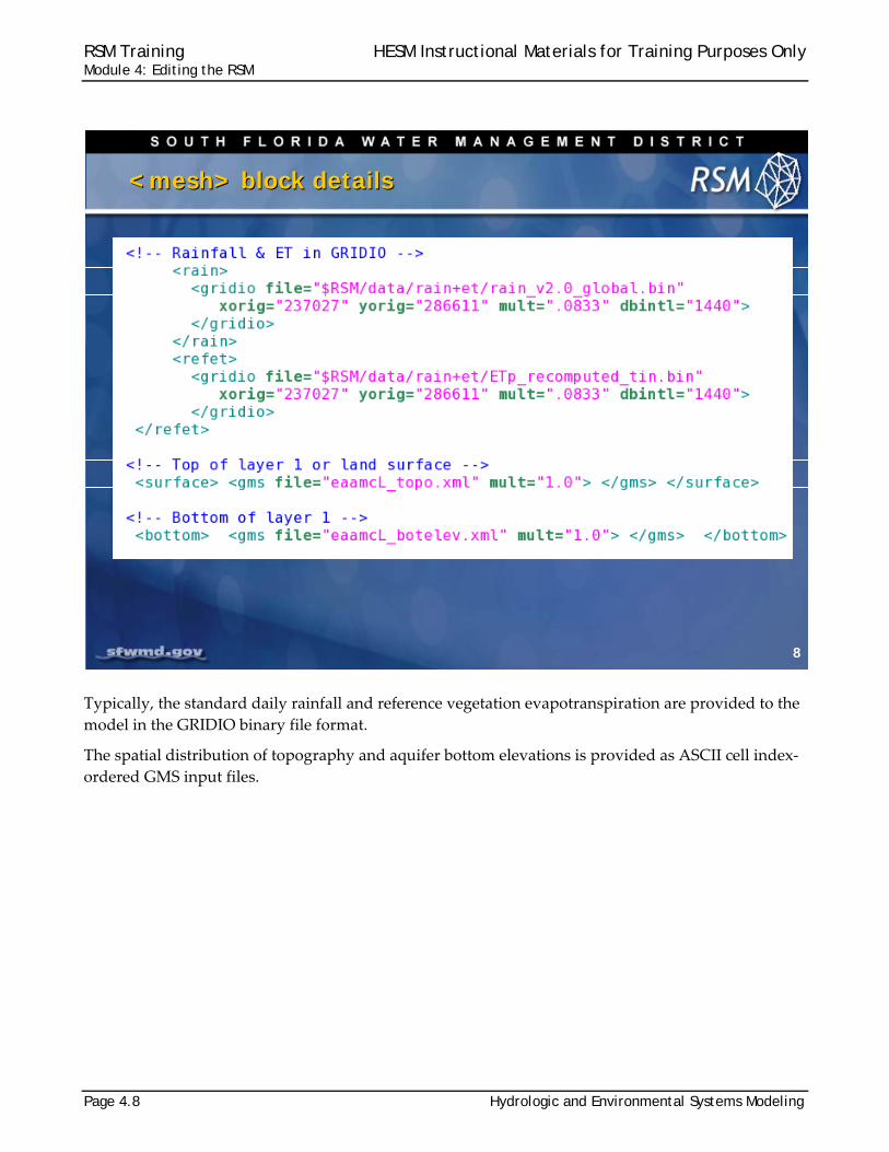
Typically, the standard daily rainfall and reference vegetation evapotranspiration are provided to the

model in the GRIDIO binary file format.

The spatial distribution of topography and aquifer bottom elevations is provided as ASCII cell index‐

ordered GMS input files.

8

<mesh> block details<mesh> block details



The source data for the mesh attributes may be provided to the model as:

constant values for simple RSM models (e.g. testbeds) fully continuous data with a unique value for each cell zonal data with fixed values for a group of cells

We use the functionality of GIS to create the spatial input files. Times series data can be provided as:

constant values rulecurves times series data in the US Army Corps of Engineers Data Storage System (DSS) format

The rulecurves are useful for inputting management schedules as boundary conditions.

9

Mesh Attributes: source dataMesh Attributes: source data

Spatial Data

• Constant

• Zonal data

• Fully continuous

Time series

• Constant

• Rule curve

• DSS files

Spatial Data

• Constant

• Zonal data

• Fully continuous

Time series

• Constant

• Rule curve

• DSS files



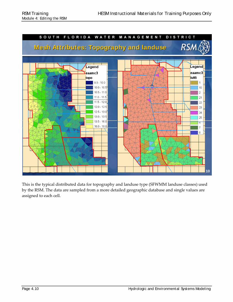
This is the typical distributed data for topography and landuse type (SFWMM landuse classes) used

by the RSM. The data are sampled from a more detailed geographic database and single values are

assigned to each cell.

10

Mesh Attributes: Topography and landuseMesh Attributes: Topography and landuse



Aquifer bottom elevation and aquifer conductivity are necessary attributes. These attributes can be

input as individual values for each cell or a single value for several cells. These values are based on

interpolated values from well core data. These data will be used in the lab exercises.

11

Mesh attributes: Mesh attributes:

Aquifer Bottom Elevation Aquifer hydraulic conductivity



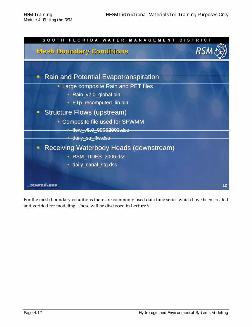
For the mesh boundary conditions there are commonly used data time series which have been created

and verified for modeling. These will be discussed in Lecture 9.

12

Mesh Boundary ConditionsMesh Boundary Conditions

Rain and Potential Evapotranspiration Large composite Rain and PET files

• Rain_v2.0_global.bin

• ETp_recomputed_tin.bin

Structure Flows (upstream) Composite file used for SFWMM

• flow_v5.0_09052003.dss

• daily_str_flw.dss

Receiving Waterbody Heads (downstream)• RSM_TIDES_2006.dss

• daily_canal_stg.dss

Rain and Potential Evapotranspiration Large composite Rain and PET files

• Rain_v2.0_global.bin

• ETp_recomputed_tin.bin

Structure Flows (upstream) Composite file used for SFWMM

• flow_v5.0_09052003.dss

• daily_str_flw.dss

Receiving Waterbody Heads (downstream)• RSM_TIDES_2006.dss

• daily_canal_stg.dss



A complete boundary condition may be specified as a general head boundary condition on a wall by a

list of nodes <nodelist> that defines the wall. It may also be specified as a general head boundary

condition for a cell and the time series of head values applied to the wall or cell.

In the first case, the time series of tidal stages are applied to the coast. In the second case, the

simulated stage values from the SFWMM are applied to a selected boundary cell.

13

Mesh Boundary conditionsMesh Boundary conditions

Complete <mesh_bc> XML Complete <mesh_bc> XML



Hydrologic Process Modules (HPMs) are used to model the local hydrology. In the simplest HPMs,

rainfall and refET are processed to calculate recharge and runoff. More complex HPMs simulate

urban and agricultural water management systems. There are several types of HPMs available for

implementation. A standard set of HPMs are used that reflect the land use/land cover types common

to south Florida.

14

Hydrologic Process ModulesHydrologic Process Modules

Process rainfall and evapotranspiration

Expression of landuse, soils and landscape

Local water management systems

Urban: irrigation, drainage, storage, and consumptive use

Agricultural: irrigation, drainage and storage

Several types:

Layer1nsm

Urban hubs: impervious land, turf & landscape, detention

Agricultural: Afsirs, ramcc

Standard set of HPMs

RSM/labs/lab11_hpm/evap_prop.xml

Process rainfall and evapotranspiration

Expression of landuse, soils and landscape

Local water management systems

Urban: irrigation, drainage, storage, and consumptive use

Agricultural: irrigation, drainage and storage

Several types:

Layer1nsm

Urban hubs: impervious land, turf & landscape, detention

Agricultural: Afsirs, ramcc

Standard set of HPMs

RSM/labs/lab11_hpm/evap_prop.xml



These standard landuse/landcover types are simulated in the RSM and used in the SFWMM.

15

Standard land use types simulated in RSMStandard land use types simulated in RSM

Land useSFWMMHPMLand useSFWMMHPM

Mixed cattail/sawgrassMIX13

Wet PrairieWET25MelalucaMEL12

Open WaterWAT24Medium Density UrbanMDU11

Sugar caneSUG23MarshMAR10

ShrublandSHR22MangroveMAN9

SawgrassSAW21Low density UrbanLDU8

Ridge & Slough 5RS520Irrigated PastureIRR7

Ridge & Slough 4RS419High Density UrbanHDU6

Ridge & Slough 3RS318Golf coursesGLF5

Ridge & Slough 2RS217Freshwater wetlands FWT4

Ridge & Slough 1RS116Forested UplandFUP3

Row cropsROW15CitrusCIT2

Open LandMLP14CattailsCAT1



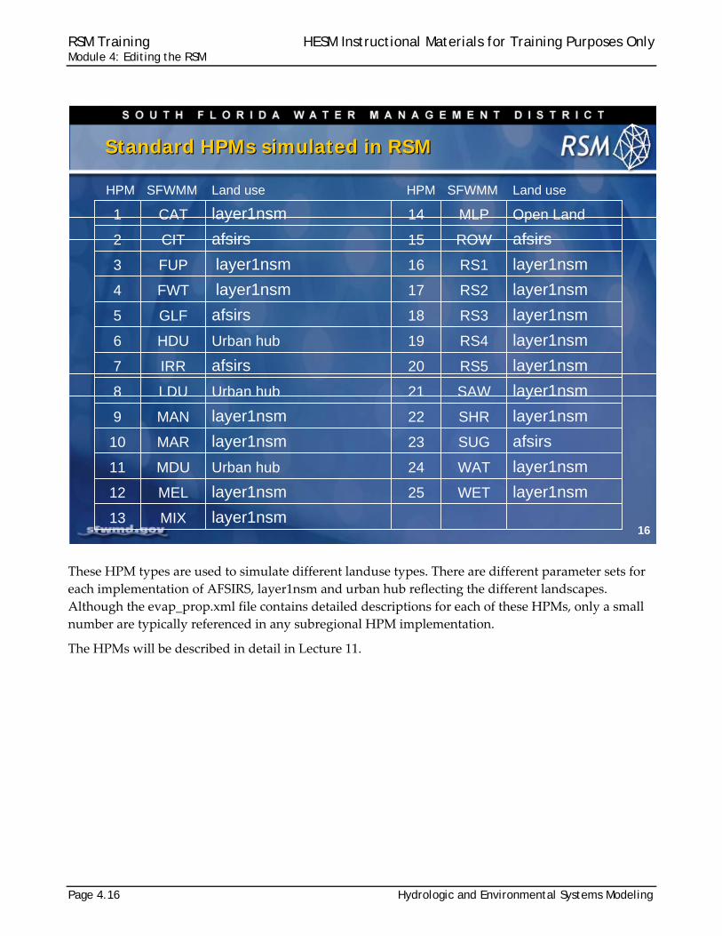
These HPM types are used to simulate different landuse types. There are different parameter sets for

each implementation of AFSIRS, layer1nsm and urban hub reflecting the different landscapes.

Although the evap_prop.xml file contains detailed descriptions for each of these HPMs, only a small

number are typically referenced in any subregional HPM implementation.

The HPMs will be described in detail in Lecture 11.

16

Standard HPMs simulated in RSMStandard HPMs simulated in RSM

Land useSFWMMHPMLand useSFWMMHPM

layer1nsmMIX13

layer1nsmWET25layer1nsmMEL12

layer1nsmWAT24Urban hubMDU11

afsirsSUG23layer1nsmMAR10

layer1nsmSHR22layer1nsmMAN9

layer1nsmSAW21Urban hubLDU8

layer1nsmRS520afsirsIRR7

layer1nsmRS419Urban hubHDU6

layer1nsmRS318afsirsGLF5

layer1nsmRS217layer1nsmFWT4

layer1nsmRS116layer1nsmFUP3

afsirsROW15afsirsCIT2

Open LandMLP14layer1nsmCAT1



The simplest HPM assignments are based on the <afsirs> and <layer1nsm> types. The <afsirs> is an

implementation of the Agricultural Field Scale Irrigation Requirements System FORTRAN program

(Smajstrla, 1990). It was created by the University of Florida to estimate optimal irrigation for many

common Florida crops, soil types and irrigation management types. The parameters for the AFSIRS

model are provided in the AFSIRS documentation (in the labs/lab11_hpm directory). The AFSIRS

model tracks soil moisture based on rain and crop evapotranspiration (ET) and calculates drainage

and irrigation requirements which are passed to the mesh cells. The AFSIRS HPM assumes that the

water table is maintained below the root zone by the RSM.

The layer1nsm HPM was adapted from the SFWMM to represent shallow wetlands where the water

table is always in the root zone or only slightly ponded. This HPM calculates ET based on the location

of the water table relative to the rooting depth (rd), extinction depth (xd), below which ET ceases; and

the ponding depth (pd) above which the HPM assumes the ET rate of shallow lake.

As each cell has an HPM assigned to it, the HPMs are assigned to each cell based on the “lu.index”

file. The lu.index file provides a list of hpmEntry id values, one row for each cell. In this instance, the

lu.index file would be a list of 23s and 10s for sugar cane and marsh cells respectively.

17

Hpm.xmlHpm.xml



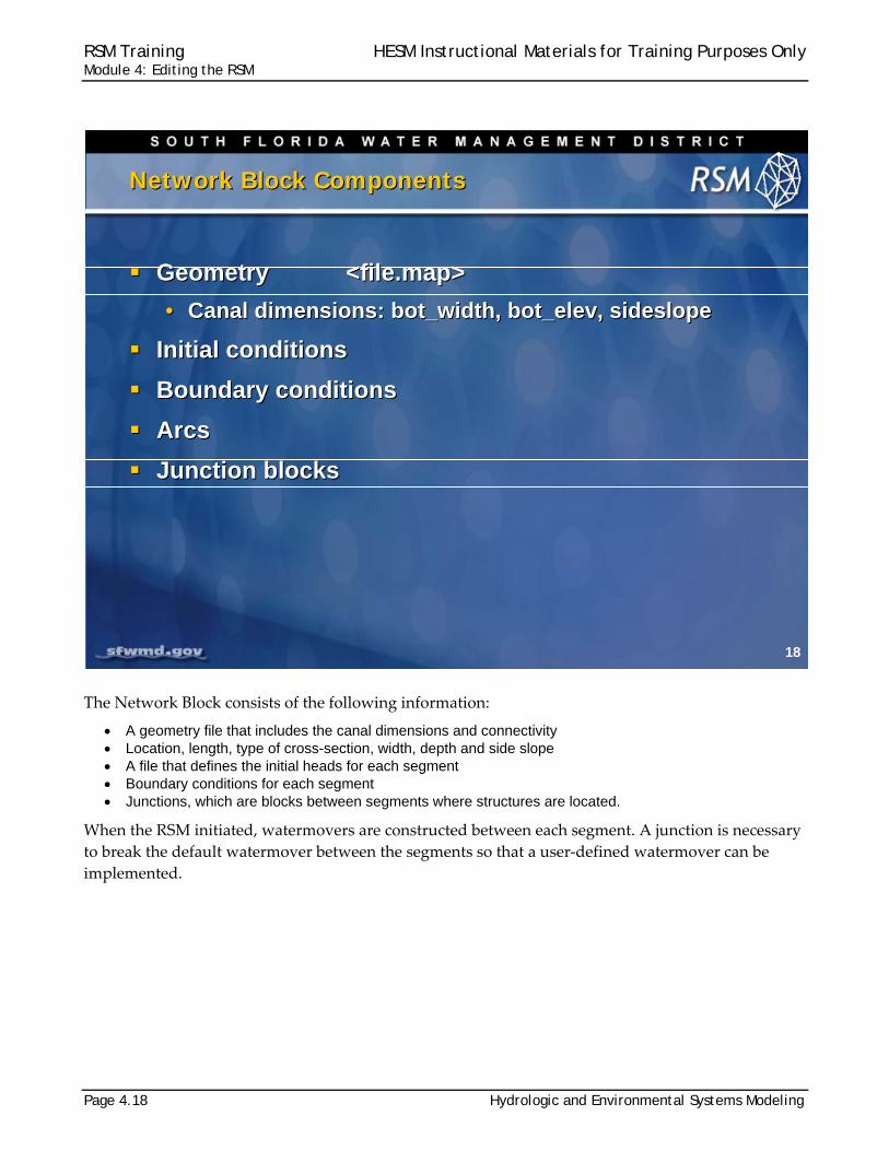
The Network Block consists of the following information:

A geometry file that includes the canal dimensions and connectivity Location, length, type of cross-section, width, depth and side slope A file that defines the initial heads for each segment Boundary conditions for each segment Junctions, which are blocks between segments where structures are located.

When the RSM initiated, watermovers are constructed between each segment. A junction is necessary

to break the default watermover between the segments so that a user‐defined watermover can be

implemented.

18

Network Block ComponentsNetwork Block Components

Geometry <file.map>

• Canal dimensions: bot_width, bot_elev, sideslope

Initial conditions

Boundary conditions

Arcs

Junction blocks

Geometry <file.map>

• Canal dimensions: bot_width, bot_elev, sideslope

Initial conditions

Boundary conditions

Arcs

Junction blocks



This is a typical XML input block for the network component of a simple RSM model. The network

block contains four elements, as described in the previous slide. The elements are as follows:

<geometry> describes the geometry of the network <initial> represents initial heads in the segments <arcs> provides the parameters for each segment in the network. These include: the Manning

roughness coefficient, leakage coefficient which characterizes exchange with the aquifer, bank height and bank coefficient which characterizes overbank flow.

<network_bc> contains the specification of the boundary conditions (BCs) for all of the reach end-segments. Typical network BCs include a flow BCs for the upper end of a canal reach and a head BC for the downstream end of a canal reach in order to form a well posed model. Other internal BCs may be applied as appropriate.

The <arcs> attributes are applied to single segments, reaches (groups of segments between structures),

or entire canals. The attributes are applied to the segments using an indexed file, “arcs.index” that

provides one set of arc attributes to each segment by placing the xentry id in the appropriate row for

each segment. For example, if there are 192 segments in the network, there will be a list of 192 rows

each containing one value. A separate <xsentry> is required for each different set of attributes.

19

<network> Block XML<network> Block XML



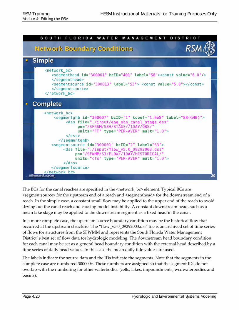
The BCs for the canal reaches are specified in the <network_bc> element. Typical BCs are

<segmentsource> for the upstream end of a reach and <segmenthead> for the downstream end of a

reach. In the simple case, a constant small flow may be applied to the upper end of the reach to avoid

drying out the canal reach and causing model instability. A constant downstream head, such as a

mean lake stage may be applied to the downstream segment as a fixed head in the canal.

In a more complete case, the upstream source boundary condition may be the historical flow that

occurred at the upstream structure. The “flow_v5.0_09292003.dss’ file is an archived set of time series

of flows for structures from the SFWMM and represents the South Florida Water Management

District’ s best set of flow data for hydrologic modeling. The downstream head boundary condition

for each canal may be set as a general head boundary condition with the external head described by a

time series of daily head values. In this case the mean daily tide values are used.

The labels indicate the source data and the IDs indicate the segments. Note that the segments in the

complete case are numbered 300000+. These numbers are assigned so that the segment IDs do not

overlap with the numbering for other waterbodies (cells, lakes, impoundments, wcdwaterbodies and

basins).

20

Network Boundary ConditionsNetwork Boundary Conditions

Simple

Complete

Simple

Complete



The specification of the values for the boundary conditions can be one of the following data types:

Constant: Data that does not change. Rulecurve: A table of paired values (date, value). The model linearly interpolates between adjacent

values. Time Series: Can be applied in a .DSS (Data Storage System) file format. The DSS format is a binary

format that was developed by the United States Army Corps of Engineers (USACE) for the storage of large volumes of time series data. We use DSSVue for rapid plotting of formatted graphs.

21

Network Boundary ConditionsNetwork Boundary Conditions

Constant <const>

Rule curve <rc>

Time series <dss>

• .DSS files (USACE Data Storage System format)

Binary, compressed

HEC_DSS utilities for processing data

DSSVue for plotting graphs

Constant <const>

Rule curve <rc>

Time series <dss>

• .DSS files (USACE Data Storage System format)

Binary, compressed

HEC_DSS utilities for processing data

DSSVue for plotting graphs



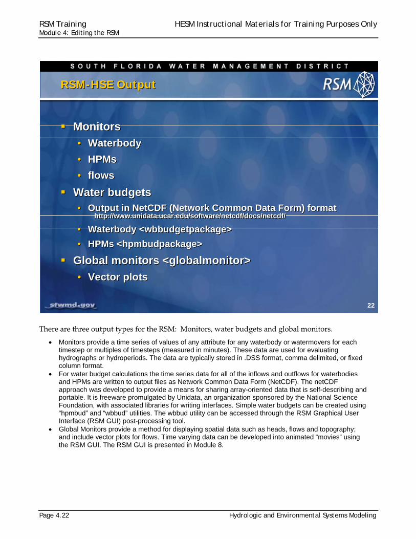
There are three output types for the RSM: Monitors, water budgets and global monitors.

Monitors provide a time series of values of any attribute for any waterbody or watermovers for each timestep or multiples of timesteps (measured in minutes). These data are used for evaluating hydrographs or hydroperiods. The data are typically stored in .DSS format, comma delimited, or fixed column format.

For water budget calculations the time series data for all of the inflows and outflows for waterbodies and HPMs are written to output files as Network Common Data Form (NetCDF). The netCDF approach was developed to provide a means for sharing array-oriented data that is self-describing and portable. It is freeware promulgated by Unidata, an organization sponsored by the National Science Foundation, with associated libraries for writing interfaces. Simple water budgets can be created using “hpmbud” and “wbbud” utilities. The wbbud utility can be accessed through the RSM Graphical User Interface (RSM GUI) post-processing tool.

Global Monitors provide a method for displaying spatial data such as heads, flows and topography; and include vector plots for flows. Time varying data can be developed into animated “movies” using the RSM GUI. The RSM GUI is presented in Module 8.

22

RSM-HSE OutputRSM-HSE Output

Monitors

• Waterbody

• HPMs

• flows

Water budgets• Output in NetCDF (Network Common Data Form) format

http://www.unidata.ucar.edu/software/netcdf/docs/netcdf/

• Waterbody <wbbudgetpackage>

• HPMs <hpmbudpackage>

Global monitors <globalmonitor>

• Vector plots

Monitors

• Waterbody

• HPMs

• flows

Water budgets• Output in NetCDF (Network Common Data Form) format

http://www.unidata.ucar.edu/software/netcdf/docs/netcdf/

• Waterbody <wbbudgetpackage>

• HPMs <hpmbudpackage>

Global monitors <globalmonitor>

• Vector plots



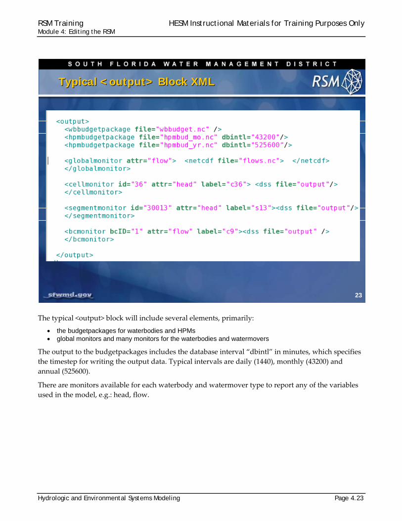
The typical <output> block will include several elements, primarily:

the budgetpackages for waterbodies and HPMs global monitors and many monitors for the waterbodies and watermovers

The output to the budgetpackages includes the database interval “dbintl” in minutes, which specifies

the timestep for writing the output data. Typical intervals are daily (1440), monthly (43200) and

annual (525600).

There are monitors available for each waterbody and watermover type to report any of the variables

used in the model, e.g.: head, flow.

23

Typical <output> Block XMLTypical <output> Block XML



Watermovers are necessary to represent structures in the RSM. There are default watermovers that

connect all of the mesh cells and network segments. Other user‐specified watermovers are necessary

to represent simulated and imposed flow at structures. The watermovers also are used to represent

levee seepage.

24

Watermovers blockWatermovers block

Default Watermovers

User-specified

• Boundary conditions

• Levee seepage

• Simulated watermovers

Weirs

Pumps (defined flow structures)

Default Watermovers

User-specified

• Boundary conditions

• Levee seepage

• Simulated watermovers

Weirs

Pumps (defined flow structures)



Two common user‐defined watermovers include the <single_control> watermover and the

<genxweir>.

The first case is a pump that is defined by the upstream stage in waterbody 295013 and the discharge

rate. For this simple case it is assumed that the downstream stage is not important. The

<single_control> watermover does not allow gravity flow through the structure or reverse flow.

The second common structure is the <genxweir>. This watermover is described in more detail in

Lecture 10.

25

Typical user-defined RSM WatermoversTypical user-defined RSM Watermovers



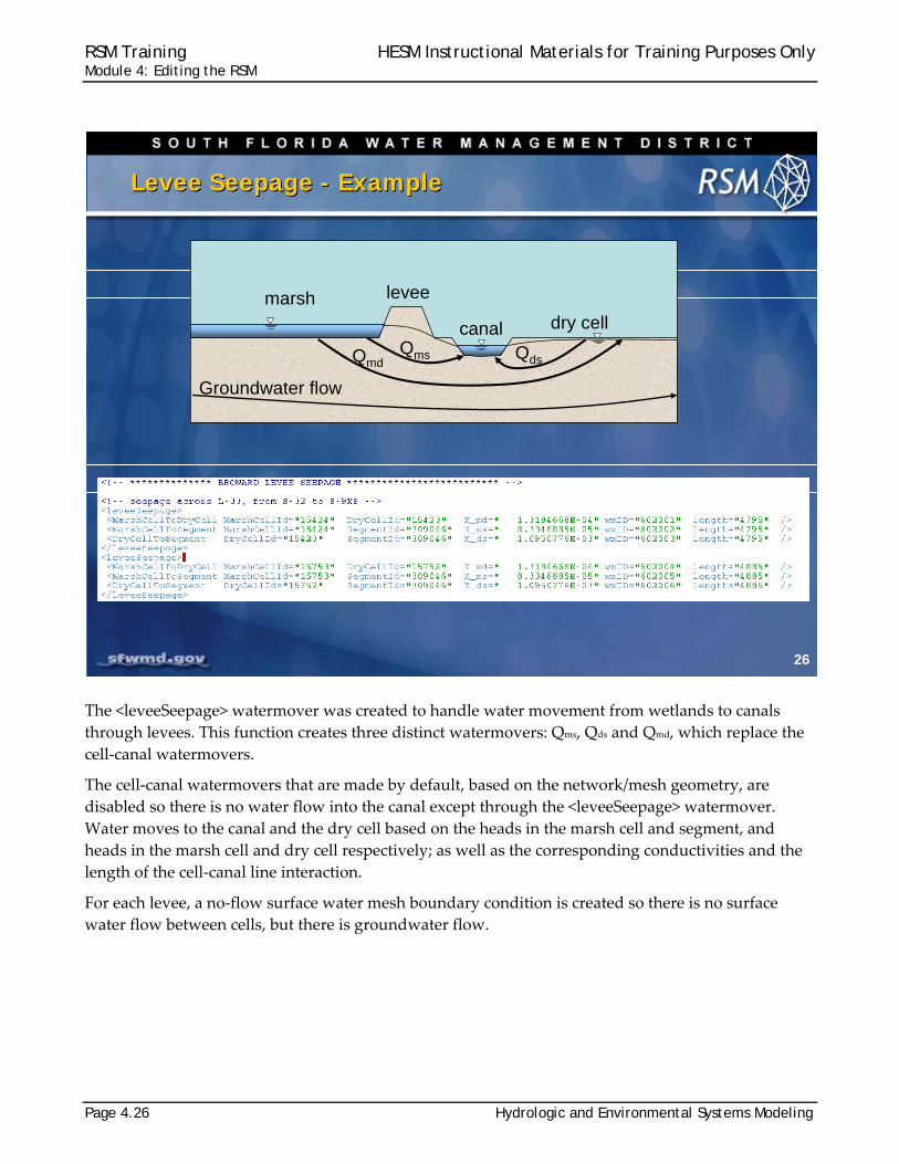
The <leveeSeepage> watermover was created to handle water movement from wetlands to canals

through levees. This function creates three distinct watermovers: Qms, Qds and Qmd, which replace the

cell‐canal watermovers.

The cell‐canal watermovers that are made by default, based on the network/mesh geometry, are

disabled so there is no water flow into the canal except through the <leveeSeepage> watermover.

Water moves to the canal and the dry cell based on the heads in the marsh cell and segment, and

heads in the marsh cell and dry cell respectively; as well as the corresponding conductivities and the

length of the cell‐canal line interaction.

For each levee, a no‐flow surface water mesh boundary condition is created so there is no surface

water flow between cells, but there is groundwater flow.

26

Levee Seepage - ExampleLevee Seepage - Example

levee

canal dry cellmarsh

Groundwater flow

QmsQmdQds



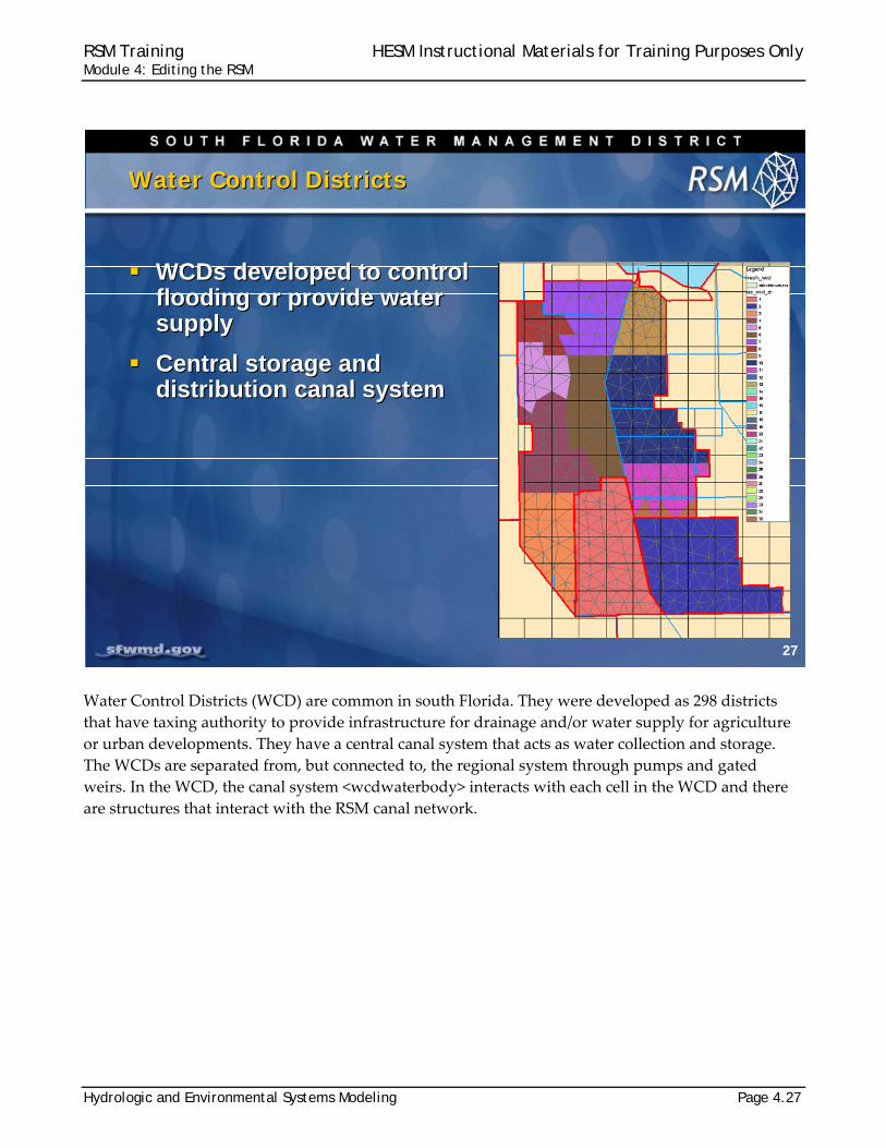
Water Control Districts (WCD) are common in south Florida. They were developed as 298 districts

that have taxing authority to provide infrastructure for drainage and/or water supply for agriculture

or urban developments. They have a central canal system that acts as water collection and storage.

The WCDs are separated from, but connected to, the regional system through pumps and gated

weirs. In the WCD, the canal system <wcdwaterbody> interacts with each cell in the WCD and there

are structures that interact with the RSM canal network.

27

Water Control DistrictsWater Control Districts

WCDs developed to control flooding or provide water supply

Central storage and distribution canal system

WCDs developed to control flooding or provide water supply

Central storage and distribution canal system



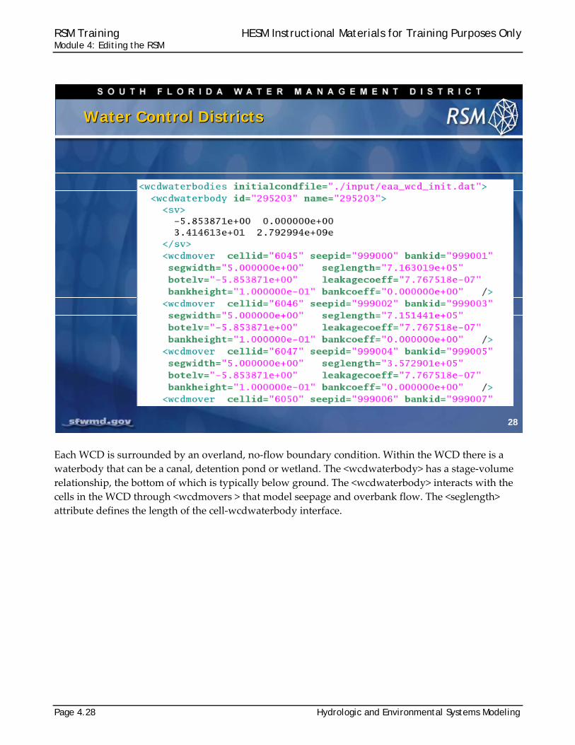
Each WCD is surrounded by an overland, no‐flow boundary condition. Within the WCD there is a

waterbody that can be a canal, detention pond or wetland. The <wcdwaterbody> has a stage‐volume

relationship, the bottom of which is typically below ground. The <wcdwaterbody> interacts with the

cells in the WCD through <wcdmovers > that model seepage and overbank flow. The <seglength>

attribute defines the length of the cell‐wcdwaterbody interface.

28




The <wcdwaterbodies> are connected with the canal network using two user‐specified watermovers,

one for inflow and one for outflow. This page includes the syntax for implementing a pair of pumps.

29




Creation of a complete RSM implementation requires a geodatabase with the necessary spatial

attribute features. An RSM implementation should begin small and add components in steps, to

obtain the necessary complexity.

For regional simulation, the available data may not support a complex model structure. The

components and the syntax for the components can be obtained from the HSE User Manual, the

benchmarks and other RSM implementations.

30

Create an RSM ImplementationCreate an RSM Implementation

Create Personal Geodatabase

Model Creation

• Create basic RSM

• Add components step-wise

• Develop components from documents:

User Manual

Benchmarks

• Adapt components from other models

Well exercised components

Create Personal Geodatabase

Model Creation

• Create basic RSM

• Add components step-wise

• Develop components from documents:

User Manual

Benchmarks

• Adapt components from other models

Well exercised components



Knowledge Assessment

1. What are the key elements of the <control> block? 2. What are the key elements of the <mesh> block? 3. How are rainfall and refET included in the model? 4. How are spatial data entered into RSM? 5. How are time series data entered into RSM? 6. What are the three groups of hydrologic process modules? 7. What is the purpose of HPMs? 8. What are elements of the <network> block?

9. What are the key components of the <output> block? 10. How does the leveeSeepage watermover work? 11. How are secondary drainage systems modeled in RSM?



Answers

1. The <control> block includes the start and end time, time step, units and MSE control parameters.

2. The <mesh> block includes the mesh topology including surface and bottom

elevations, initial head, boundary conditions including rain and refET, SV-converter, resistance terms, and HPMs.

3. The rain and refET are typically included as a “gridio” binary file that provides an

interpolated value for each mesh cell. However, rain and refET can be implemented as constants or simple time series.

4. Spatial data can be entered as 1) constant values, 2) zonal data, or 3) continuous data

using “gms” format or indexed data. 5. Time series data can be entered as constant values, waterbody-indexed, gridio, DSS

files or netCDF files. 6. The three major groups of HPMs are HPMs for urban, agricultural and native

landuse/land cover types. 7. The HPMs are implemented to model surface hydrologic processes including irrigation

and drainage that are important to the regional implementation of the model. 8. The <network> block contains the following elements:

<geometry>, topology of the canal network, <initial>, initial conditions <network_bc>, boundary conditions for the canal network <arc>, Manning’s n and canal-aquifer interaction terms.

9. The <output> block contains three elements: monitors for recording the value of any state or dynamic variable, water budgets for waterbodies and HPMs, and globalmonitors that record the value for selected state variables for every waterbody at each time step.

10. The <leveeSeepage> watermover has three watermovers: MarshtoSegment,

MarshtoDrycell and DrycelltoSegment watermovers that operate on a noflow boundary between two cells.

11. The secondary drainage systems are modeled using WCDs.



Lab 4: Build a Complete RSM

Time Estimate: 4 hours

Training Objective: Create the components of a simple RSM

A simple Regional Simulation Model can be built from components of previous RSMs.

In the case of a simple RSM, the benchmarks can be used as templates for the XML file.

In this lab, you will build a complete model for the Everglades Agricultural Area‐

Miami Canal (EAA‐MC) Basin.

In the lab exercises in Module 3, you built the mesh and the canal network. If you did

not complete building the mesh and network, the mesh and network are provided in

the following directory:

$RSM/../labs/lab4_complete_RSM directory

Lecture 4: Complete Construction of simple RSM Lecture 4: Complete Construction of simple RSM



NOTE:

For ease of navigation, you may wish to set an environment variable to the directory where you install the RSM code using the syntax

setenv RSM <path>

For SFWMD modelers, the path you should use for the NAS is:

/nw/oomdata_ws/nw/oom/sfrsm/workdirs/<username>/trunk

setenv RSM /nw/oomdata_ws/nw/oom/sfrsm/workdirs/<username>/trunk

Once you have set the RSM environment variable to your trunk path, you can use $RSM in any path statement, such as:

cd $RSM/benchmarks

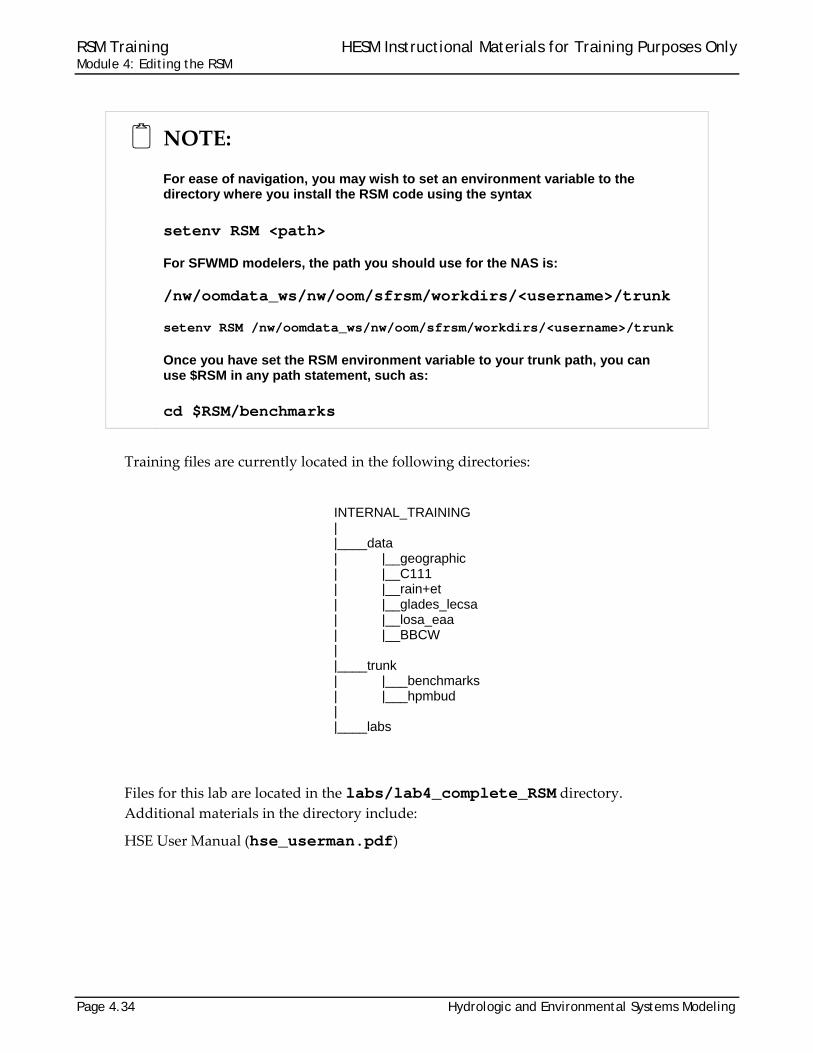
Training files are currently located in the following directories:

INTERNAL_TRAINING | |____data | |__geographic | |__C111 | |__rain+et | |__glades_lecsa | |__losa_eaa | |__BBCW | |____trunk | |___benchmarks | |___hpmbud | |____labs

Files for this lab are located in the labs/lab4_complete_RSM directory. Additional materials in the directory include:

HSE User Manual (hse_userman.pdf)



Activity 4.1: Create a Simple RSM

Overview

Activity 4.1 includes three exercises:

Exercise 4.1.1 Create a basic RSM Exercise 4.1.2 Create a simple flow condition Exercise 4.1.3 Specify different land uses

A Regional Simulation Model consists of <control>, <mesh> and <output> blocks. You

will build a simple RSM using the components from selected benchmarks.

Exercise 4.1.1 Create a basic RSM

1. From the benchmarks, search through several benchmarks to find a suitable control block

for a one-year simulation using a daily timestep.

2. Find a suitable <mesh> block that contains the required mesh elements:

<geometry> <shead> <bottom> <surface> <conveyance> <svconverter> <transmissivity>

The values for the simplest RSM should have constant values:

NOTE: Set units = “English” in the <control> block.

Bottom = -24.0 Surface = 10.0 Shead = 13.0 (flooded) Conveyance a= 0.500 dent=0.001 Transmissivity: unconfined k = 0.002 SVconverter constsv = 0.2

3. Modify the <geometry> element to include the mesh you created in Lab 3:

eaamc.2dm

4. Create the basic components of the <output> block. These include head monitors, flow

monitors and the waterbudget package.

Create a wbbudgetpackage : <wbbudgetpackage file=”wbbudget.nc”></wbbudgetpackage>

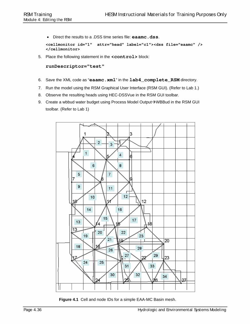
Create cell monitors for heads in a cell at the north end (Cell 1), middle (Cell 16), near south (Cell 26) and south end (Cell 30) of the model domain.



Direct the results to a .DSS time series file: eaamc.dss.

<cellmonitor id="1" attr="head" label="c1"><dss file="eaamc" /> </cellmonitor>

5. Place the following statement in the <control> block:

runDescriptor="test"

6. Save the XML code as “eaamc.xml” in the lab4_complete_RSM directory.

7. Run the model using the RSM Graphical User Interface (RSM GUI). (Refer to Lab 1.)

8. Observe the resulting heads using HEC-DSSVue in the RSM GUI toolbar.

9. Create a wbbud water budget using Process Model OutputWBBud in the RSM GUI

toolbar. (Refer to Lab 1)

Figure 4.1 Cell and node IDs for a simple EAA-MC Basin mesh.



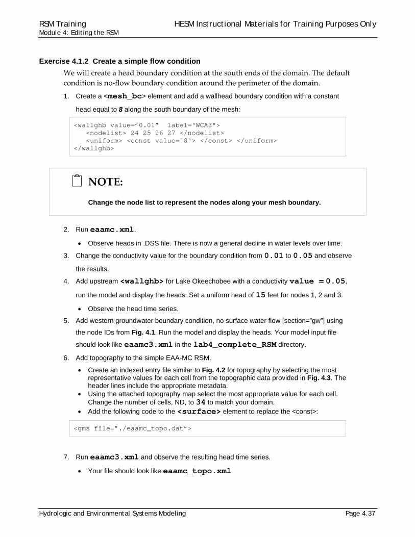
Exercise 4.1.2 Create a simple flow condition

We will create a head boundary condition at the south ends of the domain. The default

condition is no‐flow boundary condition around the perimeter of the domain.

1. Create a <mesh_bc> element and add a wallhead boundary condition with a constant

head equal to 8 along the south boundary of the mesh:

<wallghb value=”0.01” label="WCA3"> <nodelist> 24 25 26 27 </nodelist> <uniform> <const value="8"> </const> </uniform> </wallghb>

NOTE: Change the node list to represent the nodes along your mesh boundary.

2. Run eaamc.xml.

Observe heads in .DSS file. There is now a general decline in water levels over time.

3. Change the conductivity value for the boundary condition from 0.01 to 0.05 and observe

the results.

4. Add upstream <wallghb> for Lake Okeechobee with a conductivity value = 0.05,

run the model and display the heads. Set a uniform head of 15 feet for nodes 1, 2 and 3.

Observe the head time series.

5. Add western groundwater boundary condition, no surface water flow [section=”gw”] using

the node IDs from Fig. 4.1. Run the model and display the heads. Your model input file

should look like eaamc3.xml in the lab4_complete_RSM directory.

6. Add topography to the simple EAA-MC RSM.

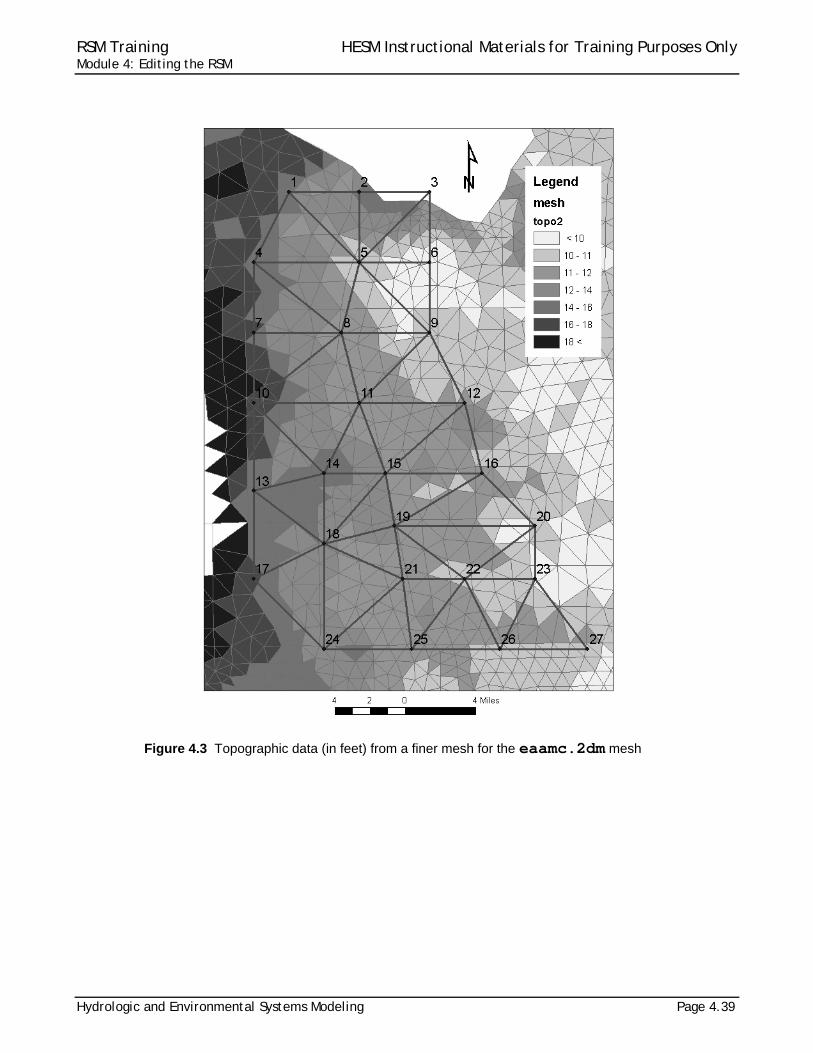
Create an indexed entry file similar to Fig. 4.2 for topography by selecting the most representative values for each cell from the topographic data provided in Fig. 4.3. The header lines include the appropriate metadata.

Using the attached topography map select the most appropriate value for each cell. Change the number of cells, ND, to 34 to match your domain.

Add the following code to the <surface> element to replace the <const>:

<gms file=”./eaamc_topo.dat”>

7. Run eaamc3.xml and observe the resulting head time series.

Your file should look like eaamc_topo.xml



DATASET # File generated by... # Program: HSE GUI HSM-1.0 # Host: # Date: 10/2/2006 # Path: topo.xml # User: unknown # Scenario: # OBJTYPE 'mesh2d' BEGSCL ND 4510 NAME 'topo' TS 0 0 25.347 24.091 25.492 …. ENDDS

Figure 4.2 Typical indexed input file



Figure 4.3 Topographic data (in feet) from a finer mesh for the eaamc.2dm mesh



a) Simple mesh with downstream boundary conditions b) Simple mesh with topography

Figure 4.4 Time series of heads for different locations in the mesh with simple boundary conditions and topography

Exercise 4.1.3 Specify different land uses

Add Hydrologic Process Modules (HPMs) to the model:

1. Change the topography back to a constant value flat condition, remove the western

boundary condition and change the Lake Okeechobee boundary condition to 13 feet.

2. Add a simple marsh HPM <layer1nsm> to the model as part of the <mesh> block.

See Benchmark 16 for details. Units for rd, xd, and pd are feet.

<hpModules> <layer1nsm kw="1.0" rd="0.5" xd="2.0" pd="3.0" kveg="0.75"/> </hpModules>



3. Add the rainfall and reference potential evapotranspiration <refet>.

The rain and refet are contained in binary files that are extracted to provide the

daily value for each mesh cell.

<rain> <gridio file="$RSM/../data/rain+et/rain_v2.0_global.bin" xorig="237027" yorig="286611" mult=".0833" dbintl="1440"> </gridio> </rain> <refet> <gridio file="$RSM/../data/rain+et/ETp_recomputed_tin.bin" xorig="237027" yorig="286611" mult=".0833" dbintl="1440"> </gridio> </refet>

4. Save file as “eaamc_hpm.xml”.

5. Run eaamc_hpm.xml and observe the resulting head time series and water budgets

(see Figure 4.5a and Table 4.1).

The cell heads vary with the seasonal rain for native land. Add the code for creating an HPM monthly budget in the <output> block:

<hpmbudgetpackage file=”hpmbudget_mon.nc” dbintl”43200”/>

The water budgets can be created for each cell using the hpmbud utility. A separate file containing the cell numbers has to be created for hpmbud.

$RSM/hpmbud/hpmbud –n hpmbudget_mo.nc –s cell2 –d –m 12

Table 4.1 Monthly water budget for Cell 16 for layer1nsm HPM for the EAA-MC basin.



6. Change the HPM from marsh to sugarcane.

Comment-out the marsh HPM (layer1nsm) using [] syntax

7. Add the sugarcane HPM code.

Create the appropriate lu.index file based on lab exercises in Module 3.

<hpModules> <indexed file=”lu.index”> <hpmEntry id="6" label="sugar - subirrigation"> <afsirs> <afcrop label="sugar" id="15" j1="01-01" jn="12-31" depth1="18" depth2="36"> <kctbl> 0.47 0.33 0.42 0.52 0.77 0.96 0.71 0.66 0.68 0.50 0.52 0.55 </kctbl> <awdtbl> 0.65 0.65 0.35 0.35 0.35 0.50 0.65 0.65 0.65 0.65 0.65 0.65 </awdtbl> </afcrop> <afirr label="SEEPAGE, SUBIRRIGATION" wtd="8.0"> <irrmeth id="7" eff="0.5" arzi="1.0" exir="1.0"></irrmeth> <irrmgmt trigcode="0"></irrmgmt> </afirr> <afsoil label="MUCK SOILS" depth="96" minwc=".20" maxwc=".50" cond="1"> </afsoil> </afsirs> </hpmEntry> </indexed> </hpModules>

Figure 4.6 The XML code for the Agricultural Field Scale Irrigation Requirements Simulation (AFSIRS): sugarcane HPM.

Save file as eaamc_sc.xml

8. Run eaamc_sc.xml with sugar cane and observe the resulting head time series and

water budgets (see Figure 4.5b and Table 4.2)..

The head time series is smoother (Fig. 4.5) as the Agricultural Field Scale Irrigation

Requirements Simulation (AFSIRS) HPM maintains a soil water budget separate from

the cell unlike the <layer1nsm>.

The HPM water budgets can be compared to values of ET, irrigation requirement and

runoff that are expected from sugarcane.



a) Simple mesh with layer1nsm HPM b) Simple mesh with sugar cane HPM

Figure 4.5 Time series for head with different cells in the simple mesh for marsh HPM and flood-irrigated sugar cane HPM

Table 4.1 Monthly water budget for Cell 16 for sugarcane HPM for the EAA-MC Basin.



Activity 4.2: Add a canal network to the EAA-MC Basin RSM

Overview

Activity 4.2 includes one exercise:

Exercise 4.2.1 Add a canal network

The simple canal network consisting of a single canal reach was created in the Lab 3.

This canal will be added to the eaamc.xml RSM and the various features will be

examined.

Exercise 4.2.1 Add a canal network

The components of the network can be found in several benchmarks, including BM4,

BM11 and BM34. For many components of the RSM, a snippet of XML script can be

copied from a reliable source, such as a benchmark, and edited as necessary.

1. Add the following network component to eaamc.xml:

<network> <geometry file="canal3x3.map"> </geometry> <initial file="canal3x3.init"> </initial> <arcs> <indexed file="arcs.index"> <xsentry id="1"> <arcflow n="0.2"></arcflow> <arcseepage leakage_coeff="0.000405" /> <arcoverbank bank_height="0.001" bank_coeff="0.001"/> </xsentry> </indexed> </arcs> </network>

2. Change the map file to eaamc.map. Also change the canal3x3.init file.

Create a new initial conditions file by copying the one from BM4 and adding the

necessary values for each of the 13 segments. The initial head can be uniformly set

to 9.0 feet.

3. Create an arcs.index file that contains the value “1” in a row for each of the 13

segments, which will apply the arc parameters to each of the segments in the network.

4. Save the file as eaamc_net.xml.

5. Run eaamc_net.xml using the RSM GUI and graph the head time series using HEC-

DSSVue.



6. Add boundary conditions.

Add a simple head <segmenthead> boundary condition element in

<network_bc> element inside <network> block for Segment 300013 (see BM10 for details).

<network_bc> <segmentghb id="300013" bcID=”1” kcoef=”0.001” label="S8 gbh"> <const value="8.0"></const> </segmentghb> </network_bc>

7. Run eaamc_net.xml.

8. Add segment head monitors to the <output> block.

<segmentmonitor id=”300013” attr=”head” label=”s300013”> <dss file=”eaanet” /> </segmentmonitor>

9. Add a flow monitor to <output> block for the segment boundary condition.

Although flow cannot be monitored in the final segment, flow can be monitored in

the boundary condition.

<bcmonitor bcID=”1” attr=”head” label=”bc1”><dss file=”eaamcnet” /> </bcmonitor>

Observe the cell and segment heads and flow. Save as eaamc_net.xml.

10. Run eaamc_net.xml.

Observe the cell and segment heads and flow.

11. Change the segment properties: Manning’s n and bottom width (eaamc.map) and

observe how they affect the EAA-MC cell heads and segment heads.

12. Change canal bed leakage (arcseepage attribute leakage_coeff) and observe how

the change affects the EAA-MC cell heads and segment heads.

13. Add HPMs to the mesh.

Compare layer1nsm HPMs to AFSIRS (sugarcane) HPMs.



a) EAA-MC RSM model without canal drainage b) EAA-MC RSM with canal drainage

c) Segment head in EAA-MC RSM d) Flow from final segment in EAA-MC RSM

Figure 4.6. Impact of simple network on heads in simple EAA-MC mesh.



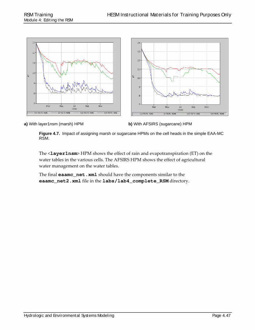
a) With layer1nsm (marsh) HPM b) With AFSIRS (sugarcane) HPM

Figure 4.7. Impact of assigning marsh or sugarcane HPMs on the cell heads in the simple EAA-MC RSM.

The <layer1nsm> HPM shows the effect of rain and evapotranspiration (ET) on the

water tables in the various cells. The AFSIRS HPM shows the effect of agricultural

water management on the water tables.

The final eaamc_net.xml should have the components similar to the

eaamc_net2.xml file in the labs/lab4_complete_RSM directory.





Answers for Lab 4

Exercise 4.1.1 2. Use components from BM16 run3x3.xml.

8. The results are constant heads, nothing is moving.

Exercise 4.1.2 1. See BM34 for syntax

6. Topography strongly affects the water flow. Changing the upstream boundary

condition does not affect the results.

Exercise 4.1.3 <no questions>

Exercise 4.2.1

11. Observe how a change in segment properties affects the EAA‐MC cell heads and

segment heads.

The changes to the canal width and Manning’s n coefficients (a and b) did not

drastically change the pattern (shape) of the head curves, providing the new values are

within a realistic range. They do, however, alter the slope of the curves (how fast they

change). As expected, higher Manning’s n values and smaller widths lead to more

pronounced differences in head between the segments and cells, while larger widths

and lower roughness damps the differences. The final heads do not vary significantly

based on changes in roughness and width.

12. Observe how a change in canal bed leakage affects the EAA‐MC cell heads and

segment heads.

As the leakage coefficient decrease the heads begin to resemble those in Figure 4.6a (no

leakage condition), where the heads decrease slower through time. However, even

large increases (original k = 0.01, new k = 10.0) do not cause significant change in the

heads.





Index AFSIRS, see also HPM ... 2, 16, 17, 42, 45,

47 aquifer ............................ 3, 6, 8, 11, 19, 32 arc parameters ....................................... 44 arcs.index file .......................................... 44 arcseepage ....................................... 44, 45 attribute .................... 11, 19, 22, 28, 30, 45 bank height ............................................. 19 basin ....................................................... 20 BBCW, see also Biscayne Bay Coastal

Wetlands ......................................... 3, 34 BC, see also input data - boundary

conditions ...................................... 19, 20 benchmark ................ 30, 33, 34, 35, 40, 44

BM16 ............................................ 40, 49 BM34 ............................................ 44, 49 BM4 .................................................... 44

Biscayne Bay Coastal Wetlands, see also BBCW ................................................... 3

bottom elevation ............................... 11, 32 C111 model ........................................ 3, 34 calibration ................................................. 3 canal ............................................. 3, 19, 26

bed leakage .................................. 45, 49 network ................... 4, 27, 29, 32, 33, 44 reach ....................................... 19, 20, 44

canal, see also WCD ... 3, 4, 18, 19, 20, 26, 27, 28, 29, 32, 33, 44, 45, 46, 49

canal3x3.init............................................ 44 cell

heads ................................ 41, 45, 47, 49 cell, see also mesh 8, 9, 10, 11, 13, 17, 20,

24, 26, 27, 28, 32, 35, 36, 37, 41, 42, 43, 45, 47, 49

cellmonitor, see also monitor ............ 35, 36 coefficient ......................................... 19, 49 components of the network .................... 44 conductivity value ................................... 37 conductivity, see also hydraulic

conductivity ................................... 11, 37 constant head ................................... 37, 49 constant values ............................. 9, 32, 35 control ............................... 4, 31, 32, 35, 36

block ............................................... 4, 35 conveyance ........................................ 6, 35 default condition ..................................... 37

drainage .......................... 17, 27, 31, 32, 46 DSS time series file ................................ 36 DSSVue ..................................... 21, 36, 44 EAA ............... 36, 37, 41, 44, 45, 46, 47, 49 EAA-MC basin .... 36, 37, 41, 44, 45, 46, 47,

49 EAA-MC model ................................ 44, 46 eaamc.2dm ...................................... 35, 39 eaamc.dss .............................................. 36 eaamc.map ...................................... 44, 45 eaamc.xml RSM ..................................... 44 effect of agricultural water management on

the water tables .................................. 47 effect of rain and evapotranspiration (ET)

on the water tables in the various cells 47 environment variable .............................. 34 ET..................................................... 17, 42 evapotranspiration, see also ET ... 8, 17, 41 Everglades Agricultural Area .................. 33 Everglades Agricultural Area-Miami Canal

(EAA-MC) Basin ................................. 33 file format ....................................... 6, 8, 21

ASCII ................................................ 6, 8 binary ...................................8, 21, 32, 41 DSS ............. 9, 20, 21, 22, 32, 36, 37, 45 NetCDF ......................................... 22, 32 XML ..... 16, 36, 37, 38, 41, 42, 44, 45, 47

flat condition ........................................... 40 flood ....................................................... 43 flow 3, 19, 20, 22, 23, 24, 26, 35, 45, 46, 49

reverse ................................................ 25 Flow from final segment in EAA-MC RSM

............................................................ 46 genxweir, see also watermover .............. 25 geodatabase .......................................... 30 geographic data ..................................... 10 GMS ..................................................... 6, 8 gravity flow ............................................. 25 groundwater ................................. 6, 26, 37

flow ..................................................... 26 gw, see groundwater .............................. 37 head . 13, 19, 20, 23, 32, 35, 36, 37, 41, 42,

43, 44, 45, 49 boundary condition ....................... 13, 20 monitor ................................................ 35

historical data ..................................... 3, 20



how to build a simple RSM ............................. 35 calibrate the model ................................ 3 Change the segment properties .......... 45 create a head boundary condition ....... 37 create a simple flow condition ....... 35, 37 create a wbbud water budget .............. 36 create an indexed entry file ................. 37 graph the head time series.................. 44 process model output .......................... 36

HPM 2, 3, 6, 14, 16, 17, 22, 23, 31, 32, 34, 40, 41, 42, 43, 45, 47 afsirs in EAA-MC application ............... 43 afsirs sugarcane .................................. 43 hub ...................................................... 16 layer1nsm . 16, 17, 40, 41, 42, 43, 45, 47 sugarcane ........................................... 43 water budget ..................... 22, 34, 41, 42

HSE ................................ 2, 4, 5, 30, 34, 38 hse.dtd file ................................................ 4 Hydrologic Process Module, see also HPM

.................................................. 6, 14, 40 Impact of simple network on heads ........ 46 impoundment .......................................... 20 inflow ...................................................... 29 initial head ............................ 18, 19, 32, 44 input data

aquifer bottom elevation .................... 6, 8 boundary conditions ... 3, 4, 9, 12, 13, 19,

20, 21, 26, 28, 32, 37, 40, 45, 49 flow ..................................................... 20

input files initial conditions ............................. 32, 44 map file ............................................... 44

irrigation requirements, see also HPM ......... 17, 42

irrigation, see also HPM ......... 2, 17, 32, 42 lake ......................................................... 20 Lake Okeechobee ............................ 37, 40 lake, see also waterbody ...... 17, 20, 37, 40 landuse ............... 10, 14, 15, 16, 32, 35, 40

native, see also HPM .................... 32, 41 types ....................................... 14, 16, 32

leakage ................................. 19, 44, 45, 49 LECSA, see also Lower East Coast

Service Area ......................................... 3 levee ............................................. 3, 24, 26

levee seepage, see also seepage 3, 24, 26, 31, 32

libraries ................................................... 22 Management Simulation Engine, see also

MSE ...................................................... 5 marsh, see also HPM - layer1nsm .. 17, 26,

40, 42, 43, 47 mesh .... 3, 4, 6, 7, 9, 12, 17, 24, 26, 31, 32,

33, 35, 36, 37, 39, 40, 41, 43, 45, 46 attributes ............................................... 9 geometry ............................................. 26 node ........................................ 13, 36, 37

mesh and network .............................. 3, 33 metadata ................................................ 37 minwc ..................................................... 42 model input, see input data ................ 4, 37 monitor .................................. 22, 23, 32, 45

bcmonitor ............................................ 45 global ...................................... 22, 23, 32

MSE ................................................... 5, 32 network . 3, 4, 19, 20, 24, 26, 31, 32, 33, 44,

45 no surface water flow ....................... 26, 37 no-flow boundary condition ... 26, 28, 32, 37 note ................................... 2, 20, 34, 35, 37 one-year simulation ................................ 35 outflow .................................................... 29 output data ...... 4, 22, 23, 31, 32, 35, 41, 45

flow monitors ................................ 35, 45 water budget .... 22, 23, 32, 35, 41, 42, 43

overbank flow ................................... 19, 28 parameter .................. 3, 4, 6, 16, 17, 19, 32

estimation, see also PEST .................... 3 PEST ........................................................ 3 plot ......................................................... 22 pond, see also lake ................................ 28 ponding .................................................. 17 porosity ..................................................... 6 pump, see also watermover ....... 25, 27, 29 Qds ......................................................... 26 Qmd ....................................................... 26 Qms ........................................................ 26 rainfall ................ 6, 8, 14, 17, 31, 32, 34, 41 reach ................................................ 19, 20 recharge ............................................. 6, 14 reference

HSE User Manual ................. 2, 4, 30, 34 Smajstrla ......................................... 2, 17



reference ET, see also ET 6, 14, 31, 32, 41 Regional Simulation Model, see also RSM

...................................................... 33, 35 regional system ...................................... 27 required mesh elements ......................... 35 RSM

implementation ................................ 4, 30 RSM GUI .............................. 22, 36, 38, 44

GIS ToolBar .......................................... 9 RSM, see also Regional Simulation Model

1, 2, 3, 4, 5, 9, 10, 15, 17, 18, 19, 22, 24, 27, 30, 31, 33, 34, 35, 36, 37, 41, 44, 46, 47

run3x3.xml .............................................. 49 runDescriptor .......................................... 36 runoff ............................................ 6, 14, 42 script ....................................................... 44 seasonal rain .......................................... 41 seepage .................................................. 28 segment

attributes ............................................. 49 boundary condition .............................. 45 head .............................................. 45, 49 head in EAA-MC RSM ........................ 46 monitor ................................................ 45 seglength ............................................ 28 segmenthead ...................................... 20 segmentsource ................................... 20

segment, see also waterbody segment 3, 18, 19, 20, 24, 26, 44, 45, 49

setenv ..................................................... 34 SFWMM ......................... 10, 13, 15, 17, 20 Shead ..................................................... 35 simple boundary conditions .................... 40 simple head ............................................ 45 simple head <segmenthead> boundary

condition ............................................. 45 Simple mesh with downstream boundary

conditions ............................................ 40 Simple mesh with topography................. 40 single_control, see also watermover ...... 25 soil ................................................ 6, 17, 42

water budget ....................................... 42 source boundary ..................................... 20 spatial distribution ..................................... 8

spatial input files ....................................... 9 stage ................................. 6, 13, 20, 25, 28 stage-volume ...................................... 6, 28 state variable .......................................... 32 streambank .............................................. 5 structure .......... 3, 18, 19, 20, 24, 25, 27, 30

S8 ....................................................... 45 subregional models ............................ 3, 16 sugarcane ....................... 17, 42, 43, 45, 47 surface elevation ...................................... 6 surface water .......................................... 26 SV, see also stage-volume ..................... 32 SVconverter ..................................... 32, 35 testbed ..................................................... 9 time series .. 3, 4, 12, 13, 20, 21, 22, 31, 32,

37, 40, 41, 42, 43 time step ............................ 4, 22, 23, 32, 35 topo, see topography ........................ 37, 38 topography ........................ 8, 10, 22, 37, 40 transmissivity ...................................... 6, 35

unconfined k ....................................... 35 uniform head .......................................... 37 upstream structure ................................. 20 USACE ................................................... 21 user specified watermover, see also

watermover ................................... 24, 29 user-specified watermover, see also

watermover ......................................... 25 utilities .............................................. 22, 41 vector ..................................................... 22 wallhead ................................................. 37 wallhead boundary condition .................. 37 Water Control District ......................... 3, 27 water supply ........................................... 27 waterbody .......... 5, 6, 20, 22, 23, 25, 28, 32 watermover 3, 18, 22, 23, 24, 25, 26, 31, 32

default ................................................. 24 WCD

wcdwaterbody ............................... 27, 28 WCD, see also Water Control District ... 27,

28, 32 weir ......................................................... 27 well ..........................................3, 11, 19, 26 wetlands ........................................... 17, 26

Documents

Complete Construction of Simple RSM · This is an example of the syntax used to describe the necessary elements of the mesh block. In each ... RSM Training HESM Instructional Materials