COMPLETE PARAMETER IDENTIFICATION OF A ROBOT

FROM PARTIAL POSE INFORMATION

Ambarish Goswami

Arthur Quaid

Michael Peshkin

Abstract

The absolute accuracy of a robot depends to a large extent on the accuracy with which its kinematic

parameters are known. Many methods have been explored for inferring the kinematic parameters

of a robot from measurements taken as it moves. Some require an external global positioning

system, usually optical or sonic. We have used instead a simple radial-distance linear transducer

(LVDT) which measures the distance from several fixed points in the workspace to the robot's

endpoint. This incomplete pose information (one dimensional rather than six dimensional) is

accumulated as the robot endpoint is moved within one or more hemispherical "shells" centered

about the fixed points. Optimal values for all of the independent kinematic parameters of the robot

can then be found.

Here we discuss the motivation, theory, implementation, and performance of this particularly easy

calibration and parameter identification method. We also address a recent disagreement in the

literature about the type of measuring system (in particular, the dimensionality of the pose

measurements) needed to fully identify a robot's kinematic parameters.

The authors are with the Department of Mechanical Engineering, Northwestern University, Evanston IL 60208.Earlier versions of this paper were presented in the 1992 IEEE International Conference on Systems, Man, andCybernetics, and the 1993 IEEE International Conference on Robotics and Automation.

Absolute Accuracy Vs. Repeatability

It is important to distinguish between the absolute accuracy and the repeatability of a robotic

manipulator. Repeatability of a robot is the precision with which its endpoint achieves a particular

pose (endpoint position and orientation) under repeated commands to the same set of joint angles.

Gear backlash, and sensor and servo precision are some of the factors affecting robot repeatability.

Absolute accuracy is the closeness with which the robot's actual pose matches the pose predicted

by its controller. A robot may have high repeatability while having low absolute accuracy. Given

the joint angles, the controller of a robot computes its endpoint location and orientation. For this it

needs an accurate description of the robot which involves many physical parameters such as link

lengths and joint offset angles. These numerical parameters make up the kinematic model of the

robot. The absolute accuracy of the robot depends on the accuracy of this model.

A high repeatability is of prime importance for a variety of robot applications such as pick and

place, spray painting, and welding. In these operations a robot is guided through the required

endpoint motions (with the help of a teach-pendant) and the corresponding joint-angles are

recorded. During actual operation, the robot "plays back" the recorded joint angles.

Tasks involving off-line planning, on the other hand depend on the absolute accuracy of the robot.

For us, accuracy issues arose in the context of employing a robotic system as a precision

positioning device in a medical operating room[15, 27] . In this application, a robot may improve

the quality of orthopedic surgery by accurately guiding a surgeon's saw. Cutting angles are

selected on the basis of measured anatomical features (e.g. bone dimensions) obtained through

preoperative CT scans. Robot accuracy is required so that the cuts performed are at the same

location and angle as the ones planned.

For various reasons, the numerical values of the kinematic parameters for a robot may not be

correct. This may be due to manufacturing tolerances, deviations such as link and joint

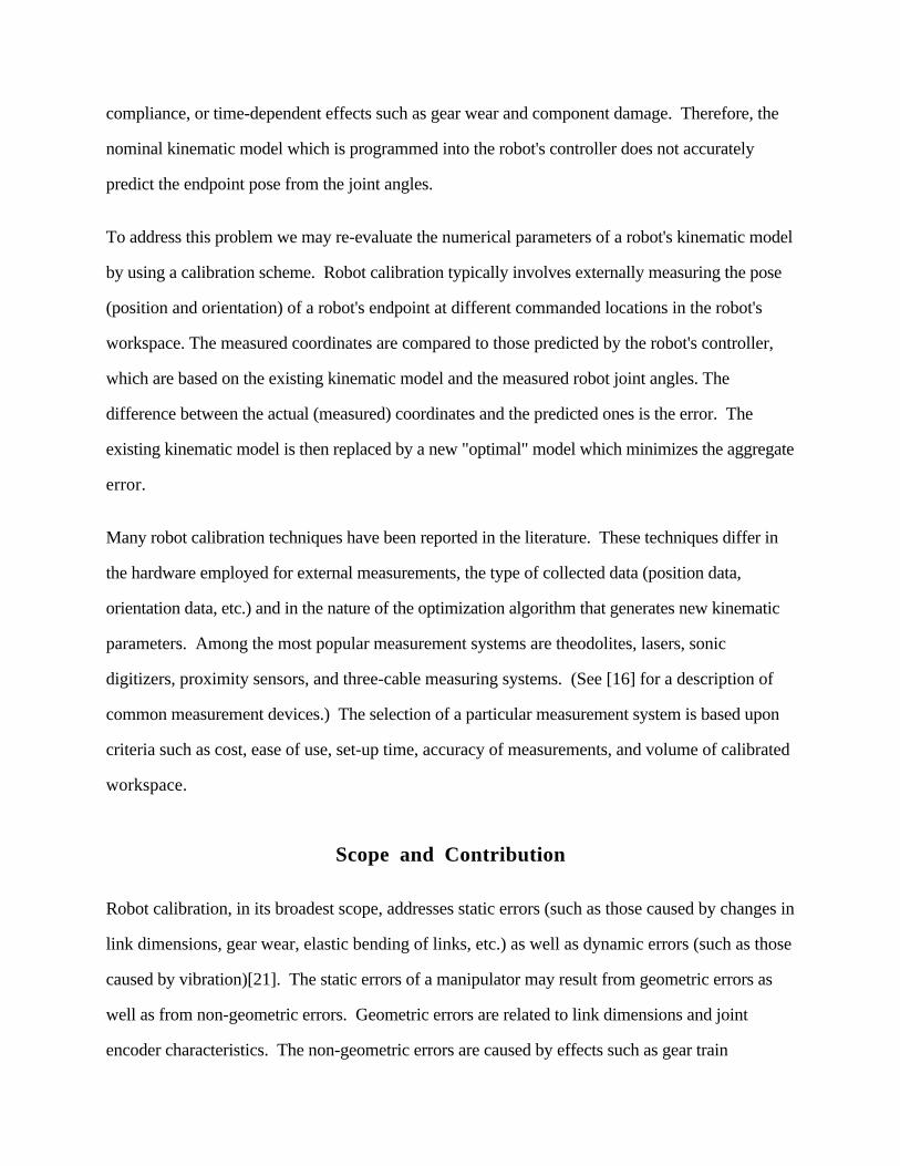
compliance, or time-dependent effects such as gear wear and component damage. Therefore, the

nominal kinematic model which is programmed into the robot's controller does not accurately

predict the endpoint pose from the joint angles.

To address this problem we may re-evaluate the numerical parameters of a robot's kinematic model

by using a calibration scheme. Robot calibration typically involves externally measuring the pose

(position and orientation) of a robot's endpoint at different commanded locations in the robot's

workspace. The measured coordinates are compared to those predicted by the robot's controller,

which are based on the existing kinematic model and the measured robot joint angles. The

difference between the actual (measured) coordinates and the predicted ones is the error. The

existing kinematic model is then replaced by a new "optimal" model which minimizes the aggregate

error.

Many robot calibration techniques have been reported in the literature. These techniques differ in

the hardware employed for external measurements, the type of collected data (position data,

orientation data, etc.) and in the nature of the optimization algorithm that generates new kinematic

parameters. Among the most popular measurement systems are theodolites, lasers, sonic

digitizers, proximity sensors, and three-cable measuring systems. (See [16] for a description of

common measurement devices.) The selection of a particular measurement system is based upon

criteria such as cost, ease of use, set-up time, accuracy of measurements, and volume of calibrated

workspace.

Scope and Contribution

Robot calibration, in its broadest scope, addresses static errors (such as those caused by changes in

link dimensions, gear wear, elastic bending of links, etc.) as well as dynamic errors (such as those

caused by vibration)[21]. The static errors of a manipulator may result from geometric errors as

well as from non-geometric errors. Geometric errors are related to link dimensions and joint

encoder characteristics. The non-geometric errors are caused by effects such as gear train

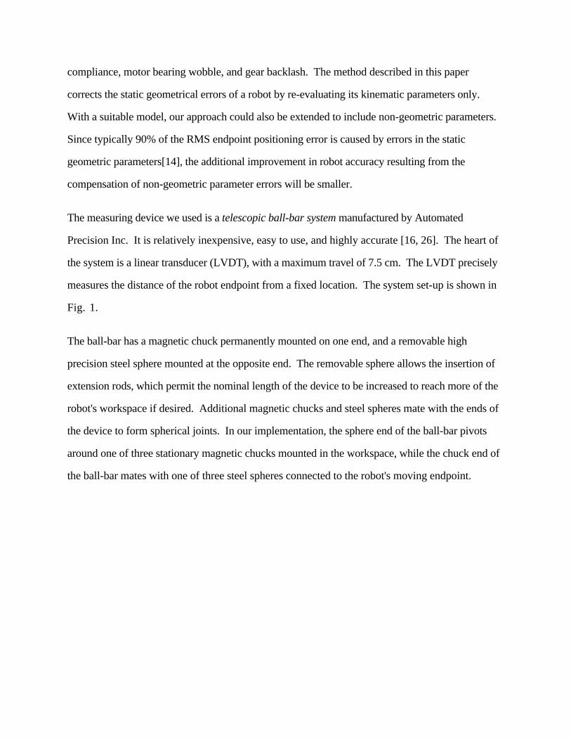
compliance, motor bearing wobble, and gear backlash. The method described in this paper

corrects the static geometrical errors of a robot by re-evaluating its kinematic parameters only.

With a suitable model, our approach could also be extended to include non-geometric parameters.

Since typically 90% of the RMS endpoint positioning error is caused by errors in the static

geometric parameters[14], the additional improvement in robot accuracy resulting from the

compensation of non-geometric parameter errors will be smaller.

The measuring device we used is a telescopic ball-bar system manufactured by Automated

Precision Inc. It is relatively inexpensive, easy to use, and highly accurate [16, 26]. The heart of

the system is a linear transducer (LVDT), with a maximum travel of 7.5 cm. The LVDT precisely

measures the distance of the robot endpoint from a fixed location. The system set-up is shown in

Fig. 1.

The ball-bar has a magnetic chuck permanently mounted on one end, and a removable high

precision steel sphere mounted at the opposite end. The removable sphere allows the insertion of

extension rods, which permit the nominal length of the device to be increased to reach more of the

robot's workspace if desired. Additional magnetic chucks and steel spheres mate with the ends of

the device to form spherical joints. In our implementation, the sphere end of the ball-bar pivots

around one of three stationary magnetic chucks mounted in the workspace, while the chuck end of

the ball-bar mates with one of three steel spheres connected to the robot's moving endpoint.

Figure 1. The calibration system with the ball-bar connected between one of three steel

spheres attached to the robot endpoint and a magnetic chuck mounted on the table.

The calibration system must read robot joint positions and LVDT lengths for various robot poses

within the workspace of the robot and within the reach of the ball-bar. Simultaneously, using

forward kinematics and the nominal robot kinematic model, the expected position of the robot

endpoint can be calculated from the joint positions. This position gives us the expected location of

the movable end of the ball-bar. The distance between the two ends is the expected ball-bar length.

The difference between the expected ball-bar length and the actual length measured by the LVDT is

the error due to incorrect robot kinematic parameters. We compute new parameters which

minimize this error.

The maximum number of independent kinematic parameters[6, 7, 8, 12], N, of a robot is given by

N = 5nr + 3np + 6 , (1)

where nr is the number of revolute joints and np is the number of prismatic joints in the robot. (In

[6, 7, 8] equation (1) was given as N = 4nr + 2np + 6 because a conversion constant for each joint

encoder was not included in the kinematic model.)

Regardless of the total number of physical parameters in the kinematic description of the robot,

which may be much larger, N is the maximum number of parameters that can be identified by

collecting data at the robot's endpoint alone. N is also the number of parameters sufficient to

compute the endpoint pose from the robot's joint angles.

A robot endpoint pose consists of endpoint position (three measurements) and orientation (three

measurements) with respect to a base coordinate frame. In order to identify a complete set of N

independent parameters of a robot, one might expect to need to measure the position and

orientation of the robot endpoint, which would require the use of a sophisticated 6-dof measuring

device. We show in this paper that a simple measuring device, capable of collecting only partial

pose information (just a radial distance) is equally effective in identifying all of the independent

robot kinematic parameters. This represents an economic and easy route to robot calibration.

Choice of a kinematic model is important for calibration; we discuss the Sheth-Uicker model

below. Next we describe the Levenberg-Marquardt algorithm which we have used for parameter

optimization, on account of its robustness and its ability to handle singular systems. We then

describe data collection and results. The final section contains a discussion of various sets of

incomplete pose information, with regard to their sufficiency or insufficiency for complete

parameter identification.

Kinematic Model

The endpoint pose (position and orientation) of a robot may be expressed as a nonlinear function of

the physical link parameters and the joint encoder parameters, which are presumed to be constants,

and of the measured joint revolute angles or prismatic displacements, which are of course

variables. The former group, the constants, comprise the kinematic parameters we seek to

identify.

Many kinematic models have been suggested. Reference [13] contains an overview of various

kinematic models in use. One has to be particularly careful in selecting a kinematic model for

calibration purposes. For instance, a model which is compact and efficient for forward and inverse

kinematics may give rise to numerical instability during parameter optimization. References [6]

and [7] discuss desirable properties of a kinematic model.

For calibration, the two most important properties of a kinematic model are completeness and

proportionality[6]. In a complete kinematic model every possible kinematic change of the robot

will be reflected by the model parameters. If we use an incomplete model for calibration and

parameter estimation, the errors in the unmodeled parameters will be partially corrected by

adjustments of physically unrelated parameters. This results in an optimized parameter set that

does not reflect the actual values of the robot's physical features, and may result in sub-optimal

robot accuracy.

Proportionality of a kinematic model requires that a small change in the physical features of a robot

is reflected by only a small change in the model parameters. Proportionality is a similar concept to

mathemetical continuity of the model parameters and ensures the numerical stability of the

optimization process.

In this work we adopt the Sheth-Uicker kinematic model [1, 22, 23]. It is complete, proportional,

and easy to assign to a manipulator. In this model three translational and three angular parameters

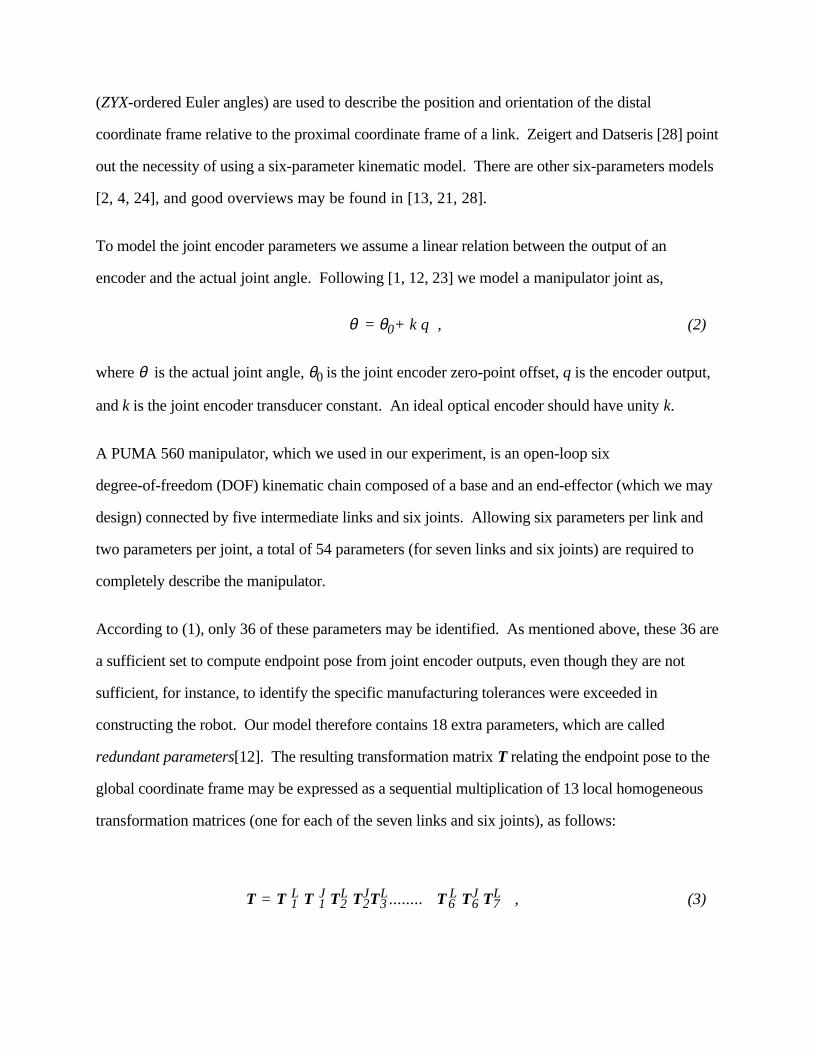
(ZYX-ordered Euler angles) are used to describe the position and orientation of the distal

coordinate frame relative to the proximal coordinate frame of a link. Zeigert and Datseris [28] point

out the necessity of using a six-parameter kinematic model. There are other six-parameters models

[2, 4, 24], and good overviews may be found in [13, 21, 28].

To model the joint encoder parameters we assume a linear relation between the output of an

encoder and the actual joint angle. Following [1, 12, 23] we model a manipulator joint as,

θ = θ0+ k q , (2)

where θ is the actual joint angle, θ0 is the joint encoder zero-point offset, q is the encoder output,

and k is the joint encoder transducer constant. An ideal optical encoder should have unity k.

A PUMA 560 manipulator, which we used in our experiment, is an open-loop six

degree-of-freedom (DOF) kinematic chain composed of a base and an end-effector (which we may

design) connected by five intermediate links and six joints. Allowing six parameters per link and

two parameters per joint, a total of 54 parameters (for seven links and six joints) are required to

completely describe the manipulator.

According to (1), only 36 of these parameters may be identified. As mentioned above, these 36 are

a sufficient set to compute endpoint pose from joint encoder outputs, even though they are not

sufficient, for instance, to identify the specific manufacturing tolerances were exceeded in

constructing the robot. Our model therefore contains 18 extra parameters, which are called

redundant parameters[12]. The resulting transformation matrix T relating the endpoint pose to the

global coordinate frame may be expressed as a sequential multiplication of 13 local homogeneous

transformation matrices (one for each of the seven links and six joints), as follows:

T = T 1L T 1

J T2L T2

JT3L........ T 6

L T6J T7

L , (3)

where T iL and T i 

Jrepresent the link transformation matrices and the joint transformation matrices,

respectively, of the ith link or joint. The global position and orientation of the endpoint can be

easily extracted from the matrix T above[11]. We use the position components to calculate the

expected length of the ball-bar: the distance from a robot endpoint-mounted steel sphere to the fixed

magnetic chuck.

Optimization

In practice, the computed distance from an endpoint-mounted steel sphere to a fixed magnetic

chuck will be different from the actual distance, as measured by the LVDT in the ball-bar. The

difference, known as the residual, is determined at many data collection points scattered throughout

the reachable workspace. The aggregate sum-of-squares of the residuals over n data collection

points, φ, is calculated as

φ = ∑i=1

n(d*(i) - dc(i)) 2 , (4)

where d*(i) and dc(i) are the measured distance and the computed distance, respectively, at the ith

data collection point. The quantity φ is used as an objective function, to be minimized by parameter

estimation to ensure the best possible manipulator accuracy.

In the following we briefly explain the mathematical formulation of the parameter estimation

scheme implemented. The multivariable objective function φ depends on all 54 kinematic

parameters, and may be expressed as the second-order expansion of a Taylor series as

φ (p + ∆p) ≅ φ (p) + gT∆p + 12 ∆pTH∆p , (5)

where p is the 54-vector of nominal parameter values and ∆p is a small perturbation of p. The 54-

vector g is the gradient of the objective function φ with respect to p. The gradient vector represents

the direction of maximum rate of change of the objective function surface and has zero magnitude

at a minimum of φ . Matrix H is the local Hessian of the objective function φ. The Hessian matrix

is a 54×54 symmetric quadratic matrix which contains information about the convexity of the

objective function. Since our kinematic model contains redundant parameters (a total of 54

parameters as opposed to 36 independent parameters) the Hessian matrix is singular. Even in a

non-redundant kinematic model, singularities may still occur if the collected data fails to excite all

the parameters.

The well known steepest descent method (also called the gradient search method) selects a

movement in p-space precisely opposite to the gradient vector g. The search technique continues

iteratively downhill until a local minimum of the objective function φ is reached. Alternatively,

under the Gauss-Newton algorithm, an iteration step is taken according to

∆p = – H–1 g , (6)

which minimizes the objective function in a small neighborhood of the current objective function

value. The step size varies inversely with the local curvature of the objective function. The

elements of the update vector ∆p are added to the corresponding elements of the parameter vector p

to give an improved set of parameters. This process continues until one or more convergence

criteria are met [19].

Although the steepest descent method is guaranteed to reach a local minimum or a saddle point, the

disadvantage of this method is that it often requires an excessively large number of iterations for

convergence. The Gauss-Newton method, on the other hand, fails whenever the Hessian matrix is

singular. It was observed by Fletcher [10] that, even in the case of positive definite Hessians,

convergence may not be assured.

A robust algorithm to solve singular systems was developed independently by Levenberg[17] and

Marquardt[18] and is known as the Levenberg-Marquardt algorithm[19, 20]. This algorithm has

been successfully used in the parametric synthesis of kinematic linkages by Tull and Lewis[25] and

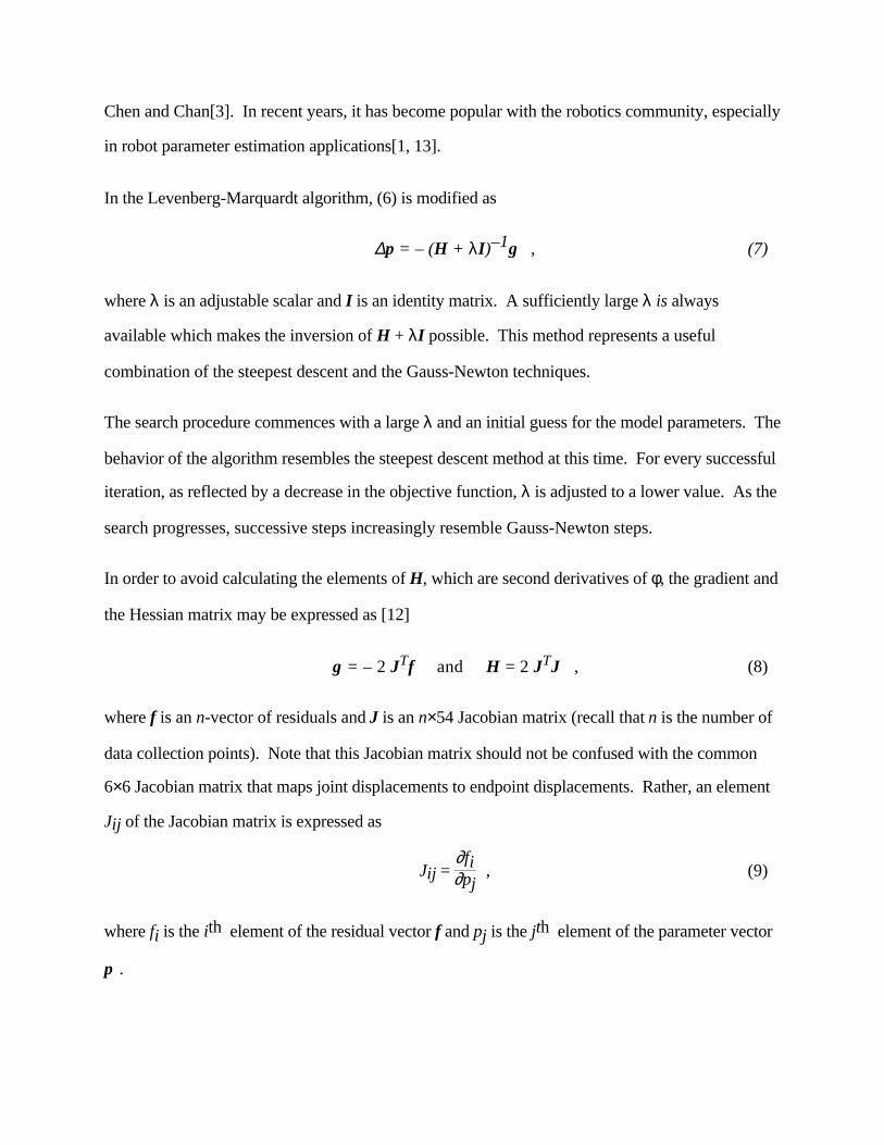
Chen and Chan[3]. In recent years, it has become popular with the robotics community, especially

in robot parameter estimation applications[1, 13].

In the Levenberg-Marquardt algorithm, (6) is modified as

∆p = – (H + λI)–1g , (7)

where λ is an adjustable scalar and I is an identity matrix. A sufficiently large λ is always

available which makes the inversion of H + λI possible. This method represents a useful

combination of the steepest descent and the Gauss-Newton techniques.

The search procedure commences with a large λ and an initial guess for the model parameters. The

behavior of the algorithm resembles the steepest descent method at this time. For every successful

iteration, as reflected by a decrease in the objective function, λ is adjusted to a lower value. As the

search progresses, successive steps increasingly resemble Gauss-Newton steps.

In order to avoid calculating the elements of H, which are second derivatives of φ, the gradient and

the Hessian matrix may be expressed as [12]

g = – 2 JTf and H = 2 JTJ , (8)

where f is an n-vector of residuals and J is an n×54 Jacobian matrix (recall that n is the number of

data collection points). Note that this Jacobian matrix should not be confused with the common

6×6 Jacobian matrix that maps joint displacements to endpoint displacements. Rather, an element

Jij of the Jacobian matrix is expressed as

Jij = ∂fi∂pj

, (9)

where fi is the ith element of the residual vector f and pj is the jth element of the parameter vector

p .

In practice, enough calibration data should be collected (more than the minimum number necessary

to solve (7), see [23]) to populate the portion of the workspace where greatest accuracy is desired.

The Jacobian matrix therefore contains many more rows (equal to the number of data points) than

columns (equal to the number of parameters).

Equation 7 may now be rewritten as

∆p = (JTJ + λI)–1(JTf) . (10)

Equation 10 is called the normal equation of this least-squares optimization. We use this equation

in error minimization.

The total number of iterations required for the convergence depends on factors such as the

topology of the objective function surface (its shallowness or its depth) and the closeness of the

initial parameter set p to the optimal set. Since our objective function is a sum of squared errors,

the topology of this surface is that of a parabolic bowl (for positive definite Hessian) or an infinite

trough (for positive semidefinite Hessian). In either case, the function surface is well conditioned

for the convergence.

If the initial parameter set p is far away from the optimal set, convergence is slower. For our

purpose, the design parameters of the manipulator, which are supplied by the manufacturer, serve

as a good initial parameter set p. In most cases convergence occurred within ten iterations.

Data Collection

Our data collection procedure involves measuring the distance of the robot endpoint from suitable

fixed positions in the robot's workspace. The single scalar distance measured falls far short of the

6-vector which would be required in order to fully determine the pose of the endpoint. It is useful

to compare our data collection "kinematics" with that of a Stewart platform. In a Stewart platform,

six linear actuators are connected between three corners of an equilateral triangular base and three

corners of an equilateral triangular platform. At any configuration the actuator lengths completely

determine the pose of the platform relative to the base[9]. We use three magnetic chucks mounted

on a equilateral triangular fixture on the robot table and imagine the fixture as the Stewart platform

base. Another fixture with three steel spheres mounted to the robot endpoint assumes the role of

the platform.

If we could simultaneously use six ball-bars to couple the fixed base to the endpoint platform we

could fully determine the 6-d endpoint pose at every robot pose. However we find it equally

effective to "serialize" the procedure by commanding the robot to travel on a hemispherical shell

(such as one shown in Fig. 2) while only one ball-bar is connected between the endpoint platform

and the fixed base. We repeat this procedure six times using different pairings of base fixture

magnetic chucks and endpoint platform steel spheres. We find we can in this way perform a

complete parameter identification with a single ball-bar at the cost of extra time.

We use the fixture shown in Fig. 1 to mount the three steel spheres to the robot endpoint. The

fixture must be such that the three spheres are not collinear. Other design concerns are low overall

weight to minimize gravity loading, and small size to minimize interferences. The fixture used to

mount the three magnetic chucks to the workspace is shown at the bottom of Fig. 1. The three

magnetic chucks must not be collinear, and the fixture should be mounted in a location such that

the hemispherical shells traced out by the ball-bar lie where the highest robot accuracy is desired.

For data collection to be automated, the ball-bar must remain connected to the robot.

Unfortunately, the limited reach of the ball-bar substantially restricts the robot endpoint’s

positional freedom. Furthermore, interference between the ball-bar and the robot-mounted fixture

must be avoided.

The net effect of these restrictions is that (as usual) the path planning cannot be done on-line using

Unimation’s VAL robot controller user interface. Path planning must be done off-line using an

external computer. We used an inverse kinematics routine based on the uncalibrated robot model

for path planning. We define positions where we wish to collect data. These positions are located

at the intersections of selected latitude and longitude lines on the hemisphere reachable by the ball-

bar at the midpoint of its travel range (see Fig. 2). Moving the robot between these data points

without exceeding the ball-bar range requires the use of intermediate path points (“via” points).

The off-line path planning must also avoid robot joint limits and singularities. The output of path

planning is a list of robot joint angle 6-vectors, each corresponding to a data collection pose or a

“via”.

Figure 2. An imaginary hemispherical shell on which the robot is programmed to travel.

Measurement takes place on each indicated data collection point.

During on-line data collection, the external program transmits the list of joint vectors to the robot

controller. The program commands the robot to sequentially move through the “via”s, stopping at

the data collection points for two seconds (to allow any dynamic oscillations to subside), before

reading the ball-bar length and the current robot joint angles (which may differ slightly from the

commanded joint angles). This information is then recorded for later use in an off-line parameter

identification program described below.

As mentioned, a minimum of six trajectories on six hemispherical shells must be used to collect

data. Since collection of excess data is always beneficial, sometime we used all nine possible ball-

bar connections. Also, we used ball-bar extension rods to collect additional sets of data on

hemispherical shells with larger radii.

Pose Measurements: How Many Dimensions Are Enough?

Duelen and Schroer[5] state that all of the kinematic parameters of a manipulator may be identified

by measuring only the position of a suitable point on the end-effector. The only requirement is that

the measurement point should not be on the axis of the robot's last joint. In our experiment,

however, we were able to identify only 33 parameters while measuring the distance of a single

endpoint-mounted steel sphere from all three fixed chucks. Measurement of the three distances is

equivalent to measuring the three Cartesian position coordinates of the steel sphere which, in fact,

is not on the robot's sixth joint axis. The three orientation parameters of the last link elude

identification in this case. A recent paper also supports our results [29]. If the endpoint-mounted

steel sphere happens to lie on the sixth joint axis we fail to identify, additionally, the error in the

sixth joint offset.

In order to evaluate the possible physical changes in any of the link geometric features or joint

encoders characteristics, the collected data must "excite" all 36 independent parameters of the

PUMA 560 robot. The number of excited (or identified) parameters is given by the number of

linearly independent columns in the Hessian matrix H or the Jacobian matrix J. Counting the

number of non-zero singular values of H or J therefore constitutes a simple test for calculating the

number of identified parameters [12, 29].

We ran several parameter identification trials with different subsets of the nine possible endpoint

platform/fixed-base pairings. The number of identified parameters for each case are shown in

Table I. The results indicate that by using all nine pairings, we can identify the complete set of 36

independent kinematic parameters. In fact any six of these nine pairings are sufficient, so long as

no steel sphere or magnetic chuck is uninvolved.

It is notable that we do not need to (and in practice we do not) cause the robot endpoint to adopt the

same set of poses for each base-platform pairing. Because of this, not a single pose can ever be

fully determined (6-dimensionally) from the data collected, but as far as parameter identification is

concerned it as if full 6-d endpoint poses were determined.

Table I: Different ball-bar pairings and the number of identified parameters

Number of spherical balls onrobot endpoint

Num

ber

of m

agne

tic

chuc

ks o

n ro

bot t

able

30 32 33

35

363533

32 34

1 2 3

1

2

3

Results and Discussion

In order to check the success of the parameter estimation process, we collected radial distance data

for two distinct sets of hemispherical shells. The radius of the first set was 46 cm, and the radius

of the second set was 61 cm, obtained by using a 15 cm extension of the ball-bar. Each set

consisted of about 800 poses. We computed the optimal parameters for the 46 cm radius set of

shells and used the new parameters to compute error residuals for the second set of shells (61 cm).

The RMS residual radial length error for the 46 cm set of shells was found to be 0.084 mm. Since

the same data was used for optimization as for error evaluation, there is an element of "mindless

curve fitting" involved. Indeed, if we had measured only 36 poses we could obtain a residual error

of zero no matter how poor the result would be on additional poses or on poses in another part of

the workspace.

To avoid both "mindless curve fitting" and also to test whether the optimized parameters work well

outside the calibrated workspace, we computed error residuals for the 61 cm shells using the robot

parameters determined for the 46 cm shell. The residual error was only 0.110 mm. This result

implies that the optimized kinematic model correctly reflects the robot geometry, and is not simply

a best fit of the data used for calibration.

Fig. 3, which shows a distribution of the final residuals on the longitudes of the data collection

hemispherical shell (see Fig. 2), demonstrates that the residuals do not vary significantly with

spatial position and thus, they reflect random errors such as repeatability and gear backlash rather

than the errors in the geometric parameters.

- 0 . 3

- 0 . 2

- 0 . 1

0 . 0

0 . 1

0 . 2

0 . 3

Res

idua

l (m

m)

0 9 0 1 8 0 2 7 0 3 6 0Longitude (degrees)

Figure 3. Plot of the distribution of the final residuals vs. longitude of the hemispherical

calibration shell.

0

20

40

60

80

freq

uenc

y

100

-0.4

-0.3

2

-0.2

4

-0.1

6

-0.0

8

0 0.08

final residuals (mm)

0.16

0.24

0.32

0.4

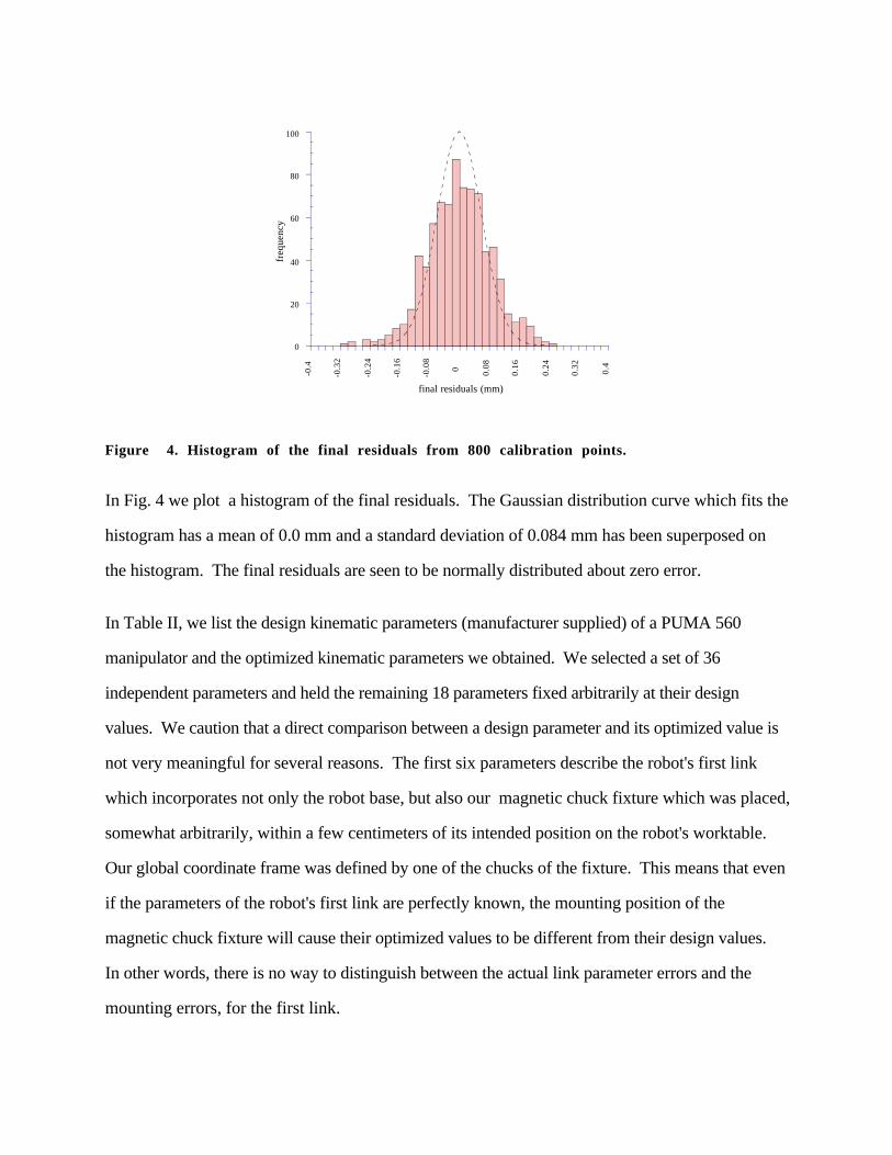
Figure 4. Histogram of the final residuals from 800 calibration points.

In Fig. 4 we plot a histogram of the final residuals. The Gaussian distribution curve which fits the

histogram has a mean of 0.0 mm and a standard deviation of 0.084 mm has been superposed on

the histogram. The final residuals are seen to be normally distributed about zero error.

In Table II, we list the design kinematic parameters (manufacturer supplied) of a PUMA 560

manipulator and the optimized kinematic parameters we obtained. We selected a set of 36

independent parameters and held the remaining 18 parameters fixed arbitrarily at their design

values. We caution that a direct comparison between a design parameter and its optimized value is

not very meaningful for several reasons. The first six parameters describe the robot's first link

which incorporates not only the robot base, but also our magnetic chuck fixture which was placed,

somewhat arbitrarily, within a few centimeters of its intended position on the robot's worktable.

Our global coordinate frame was defined by one of the chucks of the fixture. This means that even

if the parameters of the robot's first link are perfectly known, the mounting position of the

magnetic chuck fixture will cause their optimized values to be different from their design values.

In other words, there is no way to distinguish between the actual link parameter errors and the

mounting errors, for the first link.

A second caveat arises due to the redundancy of our kinematic model. Since we are forcing certain

parameters (18 of them in total) to remain fixed, any errors in the corresponding physical

dimensions will be accommodated by one or more of the other 36 parameters. Therefore, a

difference in the design value and the optimized value of a certain parameter may not necessarily

mean an actual change of the corresponding physical feature, and could equally well be due a

combined error in several other physical features.

Finally, casual readers should be warned that the optimized parameters displayed here result in

improved accuracy for our robot, with its particular manufacturing tolerances, wear, joint encoder

offset angles, etc. These parameters would not improve the performance of another robot of the

same model.

Table II: Design kinematic parameters and optimized values for a PUMA 560 manipulator

Parameters Optimized

as supplied by kinematic

the manufacturer parameters

x1 cm 0 1.25885 depends on mounting

y1 cm 0 -0.192122 depends on mounting

z1 cm 66.04 66.8858 depends on mounting

α 1 ° 0 0.0750332 depends on mounting

β1 ° 0 0.0563741 depends on mounting

γ1 ° 0 0.142109 depends on mounting

jt encoder offset 1 ° -90 -90 held fixed (#1)

jt encoder factor 1 1 0.999217

x2 cm -18 -18.0803

y2 cm 0 0.0706535

z2 cm 0 0 held fixed (#2)

α 2 ° 90 90 held fixed (#3)

β2 ° 0 -0.277037

γ2 ° -90 -90.0001

jt encoder offset 2 ° 0 0 held fixed (#4)

jt encoder factor 2 1 1.0008

x3 cm 43.18 43.3215

y3 cm 0 0.639884

z3 cm -3.091 -3.091 held fixed (#5)

α 3 ° 0 0 held fixed (#6)

β3 ° 0 -0.137778

γ3 ° 0 -0.116512

jt encoder offset 3 ° -90 -90 held fixed (#7)

jt encoder factor 3 1 1.00005

x4 cm 43.307 43.3068

y4 cm -2.032 -2.12003

z4 cm 0 0 held fixed (#8)

α 4 ° 90 90 held fixed (#9)

β4 ° 0 -0.0246447

γ4 ° 90 90.0979

jt encoder offset 4 ° 0 0 held fixed (#10)

jt encoder factor 4 1 0.998821

x5 cm 0 -0.0109964

y5 cm 0 -0.0434906

z5 cm 0 0 held fixed (#11)

α 5 ° 0 0 held fixed (#12)

β5 ° 0 -0.496135

γ5 ° -90 -90.0111

jt encoder offset 5 ° 0 0 held fixed (#13)

jt encoder factor 5 1 1.00053

x6 cm 0 0.00523043

y6 cm 0 0.0394295

z6 cm 0 0 held fixed (#14)

α 6 ° 0 0 held fixed (#15)

β6 ° 0 3.18249

γ6 ° 90 89.9855

jt encoder offset 6 ° 0 0 held fixed (#16)

jt encoder factor 6 1 1.00016

x7 cm 0 0.00166565

y7 cm 0 -0.00298551

z7 cm 5.625 5.625 held fixed (#17)

α 7 ° 0 0 held fixed (#18)

β7 ° 0 -0.0185442

γ7 ° 0 -0.00889793

Finally, it is important to distinguish between the RMS error of radial distances and the RMS error

of the robot endpoint Cartesian position. We estimated numerically the positional error of the

endpoint for a given RMS error of the radial distance. The Stewart platform analogy is again

useful here. Imagine that the robot endpoint triangle (with three steel spheres) and the base triangle

(with three magnetic chucks) are interconnected through six ball-bars in a Stewart platform

geometry. The question we then ask is: for 0.084 mm RMS errors in the ball-bars, what is the

RMS error in the positioning of the triangle?

The Jacobian matrix of a Stewart platform transforms small changes in its leg lengths to small

changes in the position of the platform [9]. For a nominal configuration of our imaginary Stewart

platform (the robot endpoint plate situated directly over the base triangle with all the ball-bars of

equal length) we computed how errors in each of its leg lengths propagate to motions of the top

platform. Using an RMS error of 0.084 mm in leg length we find the Cartesian positional error to

be roughly four times the ball-bar error, or 0.34 mm.

Conclusions

We have shown that partial pose information can be used to identify all the independent kinematic

parameters of a robot. We used a simple radial-distance transducer (an LVDT) to measure the

distance of the robot endpoint from fixed points in the workspace. Our procedure represents an

easy and economic way of calibrating a robot.

Acknowledgments

We would like to thank James Bosnik of Drexel University for useful discussions, especially in

regard to the idea of the robot endpoint fixture. Support for this research was provided by

Northwestern University, Northwestern Memorial Hospital and the NSF PYI Grant DMC-

8857854. Kornel Ehmann of Northwestern University drew our attention to the use of ball-bar for

calibration purpose. Kam Lau of Automated Precision Inc. was instrumental in making the ball-

bar device available to us at a subsidized price.

References

1. Bosnik, J. R. "Static and Vibrational Kinematic Parameter Estimation for Calibration of

Robotic Manipulators." Ph. D. Thesis, Pennsylvania State University, University Park, PA

(1986)

2. Broderick, P. L. and R. J. Cipra. A Method for Determining and Correction of Robot

Position and Orientation Errors Due to Manufacturing. ASME Journal of Mechanisms,

Transmissions, and Automation in Design 110:3-10 (1988)

3. Chen, F. Y. and V.-L. Chan. Dimensional Synthesis of Mechanisms for Function

Generation Using Marquardt's Compromise. ASME Journal of Engineering for Industry

96(1):1312-137 (1974)

4. Chen, J. and L. M. Chao. "Positioning Error Analysis for Robot Manipulators with All

Rotary Joints." Proceedings of IEEE International Conference of Robotics and Automation. (1011-

1016) IEEE Press (1986)

5. Duelen, G. and K. Schroer. Robot Calibration—Method and Results. Robotics and

Computer-Integrated Manufacturing Vol. 8(No. 4):223-231 (1991)

6. Everett, L. J., M. Driels and B. W. Mooring. "Kinematic Modelling for Robot

Calibration." Proceedings of IEEE International Conference of Robotics and Automation. (183-

189) IEEE Press (1987)

7. Everett, L. J. and T.-W. Hsu. The Theory of Kinematic Parameter Identification for

Industrial Robots. ASME Journal of Dynamic Systems, Measurement, and Control Vol. 110,

March:96-100 (1988)

8. Everett, L. J. and A. H. Suryohadiprojo. "A Study of Kinematic Models for Forward

Calibration of Manipulators." Proceedings of IEEE International Conference of Robotics and

Automation. Philadelphia, PA (798-800) IEEE Press (1988)

9. Fichter, E. F. A Stewart Platform Based Manipulator: General Theory and Practical

Construction. Int'l J. Robotics Research 5(2):157-182 (1986)

10. Fletcher, R. Practical Methods of Optimization. John Wiley and Sons, Inc.,. New York

(1980)

11. Fu, K. S., R. C. Gonzalez and C. S. G. Lee. Robotics: Control, Sensing, Vision, and

Intelligence. McGraw-Hill. New York, NY (1987)

12. Goswami, A. and J. R. Bosnik. On a Relationship between the Physical Features of

Robotic Manipulators and the Kinematic Parameters Produced by Numerical Calibration. ASME

Journal of Mechanical Design (in press) (1993)

13. Hollerbach, J. M. "A Survey of Kinematic Calibration ." The Robotics Review 1. al.

ed. MIT Press. Cambridge, MA (1989)

14. Judd, R. P. and A. B. Knasinski. "A Technique to Calibrate Industrial Robots with

Experimental Verification." Proceedings of IEEE International Conference of Robotics and

Automation. (351-357) IEEE Press (1987)

15. Kinzle, T. C., S. D. Stulberg, M. Peshkin, A. Quaid and C.-H. Wu. "An Integrated CAD-

Robotics System for Total Knee Replacement Surgery." IEEE Conference on Systems, Man, and

Cybernetics. Chicago IEEE Press (1992)

16. Lau, K., N. Dagalakis and D. Myers. "Testing ." International Encyclopedia of

Robotics: Applications and Automation. Dorf ed. John Wiley and Sons. New York (1984)

17. Levenberg, K. A Method for the Solution of Certain Non-Linear Problems in Least-

Squares. Quarterly of Applied Mathematics-Notes 2(2):164-168 (1944)

18. Marquardt, D. W. An Algorithm for Least-Squares Estimation of Nonlinear Parameters.

Journal of the Society for Industrial and Applied Mathematics 11(2):431-441 (1963)

19. Nash, J. C. Compact Numerical Methods for Computers: Linear Algebra and Function

Minimization. John Wiley and Sons, Inc. New York, NY (1979)

20. Press, W. H., B. P. Flannery, S. A. Teukolsky and W. T. Vetterling. Numerical Recipes,

The Art of Scientific Computing. Cambridge University Press. Cambridge, U.K. (1985)

21. Roth, Z., B. W. Mooring and B. Ravani. An Overview of Robot Calibration. IEEE

Transactions of Robotics and Automation RA-3(5):377-385 (1987)

22. Sheth, P. N. and J. J. Uicker. A Generalized Symbolic Notation for Mechanisms. ASME

Journal of Engineering for Industry 93(1):102-112 (1971)

23. Sommer, H. J. and N. R. Miller. A Technique for the Calibration of Instrumented Spatial

Linkages Used for Biomechanical Kinematic Measurements. Journal of Biomechanics 14(2):91-98

(1981)

24. Stone, H. W. Kinematic Modeling, Identification, and Control of Robotic Manipulators.

Kluwer. Norwell, MA (1987)

25. Tull, H. G. and D. W. Lewis. Three Dimensional Kinematic Synthesis. ASME Journal of

Engineering for Industry 90(3):481-484 (1968)

26. Vira, K. and K. Lau. "Design and Testing of an Extensible Ball Bar for Measuring the

Positioning Accuracy and Repeatibility of Industrial Robots." NAMRAC Conference. (583-590)

(1986)

27. Wu, C. H., J. Papaiannou, T. C. Kienzle and S. D. Stulberg. "A CAD-Based Human

Interface for Preoperative Planning of Total Knee Surgery." IEEE Conference on Systems, Man,

and Cybernetics. Chicago IEEE Press (1992)

28. Zeigert, J. and P. Datseris. "Basic Considerations for Robot Calibration." Proceedings of

IEEE International Conference of Robotics and Automation. Philadelphia, PA (932-938) IEEE

Press (1988)

29. Zhuang, H., Z. S. Roth and F. Hamano. Observability Issues in Kinematic Identification

of Manipulators. ASME Journal of Dynamic Systems, Measurement, and Control

Vol.114(June):319-322 (1992)