Embed Size (px)
Citation preview

Complexity Management in Graphical Models
DOCTORAL THESIS
FOR THEDEGREE OFADOCTOR OFINFORMATICS
AT THE FACULTY OF ECONOMICS,BUSINESSADMINISTRATION AND
INFORMATION TECHNOLOGY
OF THE
UNIVERSITY OF ZURICH
byTOBIAS REINHARD
fromHorw LU
Accepted on the recommendation of
PROF. DR. M. GLINZ
PROF. DR. H. C. GALL
2010

The Faculty of Economics, Business Administration and Information Technology of the Uni-versity of Zurich herewith permits the publication of the aforementioned dissertation withoutexpressing any opinion on the views contained therein.
Zurich, October 27, 20101
The Vice Dean of the Academic Program in Informatics: Prof. Dr. H. C. Gall
1Date of the graduation

iii
Abstract
Graphical or visual representations play a central role in the software life cycle as a means tomake the immaterial software more tangible and accessible.While such drawings or diagramsfacilitate a “computational offloading” when reasoning about a system, the complexity of today’ssoftware systems makes them often extremely big and cluttered. One way to cope with thissize and complexity is to use hierarchical and aspectual decompositions to split the models intomanageable and understandable parts. Such a decompositionmechanism is the basic idea behindthe ADORA approach: It uses an integrated, inherently hierarchical model together with a toolthat generates abstractions in the form of diagrams of manageable complexity. The underlyingcomplexity management mechanism combines two concepts: (i) a fisheye zoom visualizationwhich shows local detail and its surrounding global contextin one single view and (ii) a dynamicgeneration of different views by filtering specific model elements.
The work at hand covers the technical foundations of this complexity management mechanism.While the simplicity of the basic concept contributes largely to its appeal, the actual realization ina computer-based tool has to cope with a lot of conceptual andtechnical problems and trade-offs.Besides the presentation and discussion of the actual data structures and algorithms, the detailedrequirements they have to fulfill are covered as well. An improved fisheye zoom algorithm thatemploys the concept of interval scaling and solves the problem of having a user-editable layoutwhich is stable under multiple zoom operations builds the basis for the dynamic adaption ofa diagram. This algorithm can be extended to adapt the layoutif model elements are filteredto generate different views on the model. Additionally, it can be used to support the modelediting by adapting the layout automatically. Since these automatic layout adjustments result ina dynamic, constantly changing diagram, the links or lines connecting model elements have tobe adapted, too. As a solution to that problem, an automatic line routing algorithm that producesan aesthetically appealing layout and routes in real time has been developed. The basic datastructure of this algorithm can also be used to automatically place the labels accompanying thelinks.


v
Zusammenfassung
Graphische Repräsentationen spielen im Software Lebenszyklus eine zentrale Rolle dabei, im-materielle Software fassbarer und zugänglicher zu machen.Obwohl solche Grafiken oder Dia-gramme das sogenannte “computational offloading” beim Verstehen eines Systems fördern, führtdie Komplexität heutiger Softwaresysteme oftmals zu sehr grossen und überladenen Modellen.Eine Möglichkeit um dieser Grösse und Komplexität Herr zu werden liegt in einer hierarchis-chen und aspekt-basierten Dekomposition des Modells in handhabbare und verständliche Teile.Eine solche Dekomposition ist die grundlegende Idee hinterADORA: Der Ansatz beruht aufeinem integrierten, inhärent hierarchischen Modell zusammen mit einem Werkzeug, welchesAbstraktionen in der Form von Diagrammen handhabbarer Grösse und Komplexität generiert.Der Mechanismus zur Handhabung der Komplexität kombiniertzwei Konzepte: a) eine sogenan-nte Fischaugen-Visualisierung, welche lokale Details zusammen mit dem umgebenden Kontextin einer einzigen Ansicht darstellt, und b) eine dynamischeGenerierung verschiedener Sichtendurch das Ausblenden spezifischer Modellelemente.
Die vorliegende Arbeit beschäftigt sich mit den technischen Grundlagen dieses Ansatzes desUmgangs mit Komplexität. Obwohl die Einfachheit des Konzepts einen grossen Teil dessenAttraktivität ausmacht, tauchen bei der Realisierung in einem rechnergestützten Werkzeug eineganze Menge technischer Probleme und Zielkonflikte auf. Neben der Präsentation und Diskus-sion der dafür benötigen Datenstrukturen und Algorithmen,werden auch die Anforderungen,welche diese zu erfüllen haben, behandelt. Ein verbesserter Fischaugen Zoomalgorithmus, derauf dem Prinzip der Skalierung von Intervallen beruht und sowohl die Editierbarkeit des Lay-outs als auch dessen Stabilität bei mehreren Zoomoperationen garantiert, bildet die Basis fürdie dynamische Anpassung des Layouts. Dieser Algorithmus kann, mit kleinen Anpassungen,auch dazu verwendet werden, das Layout beim Generieren verschiedener Sichten durch das Aus-blenden spezifischer Modellelemente anzupassen. Zusätzlich unterstützt er den Benutzer beimEditieren des Modells durch eine automatische Anpassung. Da diese automatischen Veränderun-

vi
gen des Layouts in dynamischen, sich ständig ändernden Diagrammen resultieren, müssen auchdie Linien, welche die Modellelemente verbinden, angepasst werden. Als Lösung für diesesProblem wurde ein automatischer Linienführungsalgorithmus entwickelt, der in Echtzeit äs-thetisch ansprechende Linien generiert. Die Datenstruktur dieses Algorithmus kann zusätzlichauch zur automatischen Platzierung von Linienbeschriftungen verwendet werden.

CONTENTS vii
Contents
List of Figures xiii
I Introduction and Background 1
1 Introduction 3
1.1 Motivation. . . . . . . . . . . . . . . . . . . . . . . . . . . . . . . . . . . . . . 3
1.2 Goals and Contributions. . . . . . . . . . . . . . . . . . . . . . . . . . . . . . . 4
1.3 Thesis Outline. . . . . . . . . . . . . . . . . . . . . . . . . . . . . . . . . . . . 6
2 Graphical Modeling 9
2.1 Models and Their Representation. . . . . . . . . . . . . . . . . . . . . . . . . . 9
2.2 Graphical Models in Software Engineering. . . . . . . . . . . . . . . . . . . . . 14
2.3 Tool Support for the Modeling Process. . . . . . . . . . . . . . . . . . . . . . . 21
2.4 Aesthetics in Diagrams. . . . . . . . . . . . . . . . . . . . . . . . . . . . . . . 24
2.5 Secondary Notation and Mental Map. . . . . . . . . . . . . . . . . . . . . . . . 25
3 Complexity of Graphical Models 27

viii CONTENTS
3.1 Flat Models . . . . . . . . . . . . . . . . . . . . . . . . . . . . . . . . . . . . . 28
3.2 Horizontal Abstraction . . . . . . . . . . . . . . . . . . . . . . . . . . . . . . . 35
3.3 Vertical Abstraction. . . . . . . . . . . . . . . . . . . . . . . . . . . . . . . . . 36
4 ADORA 45
4.1 The ADORA Language . . . . . . . . . . . . . . . . . . . . . . . . . . . . . . . 45
4.2 The ADORA Tool . . . . . . . . . . . . . . . . . . . . . . . . . . . . . . . . . . 49
II Fisheye Zooming 51
5 Desired Properties of a Zoom Algorithm 53
5.1 Compact Layout. . . . . . . . . . . . . . . . . . . . . . . . . . . . . . . . . . . 53
5.2 Disjoint Nodes. . . . . . . . . . . . . . . . . . . . . . . . . . . . . . . . . . . . 54
5.3 Preserve the Mental Map. . . . . . . . . . . . . . . . . . . . . . . . . . . . . . 55
5.4 Layout Stability . . . . . . . . . . . . . . . . . . . . . . . . . . . . . . . . . . . 58
5.5 Permit Editing Operations. . . . . . . . . . . . . . . . . . . . . . . . . . . . . . 59
5.6 Runtime . . . . . . . . . . . . . . . . . . . . . . . . . . . . . . . . . . . . . . . 60
5.7 Multiple Focal Points. . . . . . . . . . . . . . . . . . . . . . . . . . . . . . . . 60
5.8 Smooth Transitions. . . . . . . . . . . . . . . . . . . . . . . . . . . . . . . . . 61
5.9 Small Interaction Overhead. . . . . . . . . . . . . . . . . . . . . . . . . . . . . 61
5.10 Minimal Node Size. . . . . . . . . . . . . . . . . . . . . . . . . . . . . . . . . 62
6 Existing Fisheye Zoom Techniques 63
6.1 The Force-Scan Algorithm. . . . . . . . . . . . . . . . . . . . . . . . . . . . . 64
6.2 SHriMP . . . . . . . . . . . . . . . . . . . . . . . . . . . . . . . . . . . . . . . 65
6.3 Berner . . . . . . . . . . . . . . . . . . . . . . . . . . . . . . . . . . . . . . . . 70
6.4 The Continuous Zoom. . . . . . . . . . . . . . . . . . . . . . . . . . . . . . . 71

CONTENTS ix
7 Zoom Algorithm 77
7.1 Data Structure. . . . . . . . . . . . . . . . . . . . . . . . . . . . . . . . . . . . 78
7.2 Zoom Operations. . . . . . . . . . . . . . . . . . . . . . . . . . . . . . . . . . 80
7.3 Bottom-up Zooming. . . . . . . . . . . . . . . . . . . . . . . . . . . . . . . . . 87
8 Dynamically Generated Views 89
8.1 Node Filters. . . . . . . . . . . . . . . . . . . . . . . . . . . . . . . . . . . . . 90
8.2 Filter Operation. . . . . . . . . . . . . . . . . . . . . . . . . . . . . . . . . . . 90
9 Editing Support 95
9.1 Inserting Nodes. . . . . . . . . . . . . . . . . . . . . . . . . . . . . . . . . . . 96
9.2 Removing Nodes. . . . . . . . . . . . . . . . . . . . . . . . . . . . . . . . . . 101
9.3 Changing the Bounds of a Node. . . . . . . . . . . . . . . . . . . . . . . . . . 103
9.4 Compacting Nodes. . . . . . . . . . . . . . . . . . . . . . . . . . . . . . . . . 103
10 Discussion of the Zoom Algorithm 105
10.1 Properties of the Zoom Algorithm. . . . . . . . . . . . . . . . . . . . . . . . . 105
10.2 Algorithmic Complexity . . . . . . . . . . . . . . . . . . . . . . . . . . . . . . 116
III Line Routing 117
11 Lines in Graphical Models 119
11.1 Lines in Hierarchical Models. . . . . . . . . . . . . . . . . . . . . . . . . . . . 119
11.2 Lines in a Dynamic Layout. . . . . . . . . . . . . . . . . . . . . . . . . . . . . 122
11.3 Desired Properties of a Line Routing Algorithm. . . . . . . . . . . . . . . . . . 123
12 Existing Line Routing Approaches 129
12.1 Lines as Part of the Automatic Graph Drawing. . . . . . . . . . . . . . . . . . . 129

x CONTENTS
12.2 Routing on the Visibility Graph. . . . . . . . . . . . . . . . . . . . . . . . . . . 130
12.3 Grid-Based Routing. . . . . . . . . . . . . . . . . . . . . . . . . . . . . . . . . 131
12.4 Routing in Incremental Layouts. . . . . . . . . . . . . . . . . . . . . . . . . . . 133
13 Tile Maze Router 135
13.1 Data Structure. . . . . . . . . . . . . . . . . . . . . . . . . . . . . . . . . . . . 135
13.2 Channel Finding. . . . . . . . . . . . . . . . . . . . . . . . . . . . . . . . . . . 141
13.3 Bend Points Calculation. . . . . . . . . . . . . . . . . . . . . . . . . . . . . . . 143
13.4 Line Crossings. . . . . . . . . . . . . . . . . . . . . . . . . . . . . . . . . . . . 147
13.5 Calculation of the Start and End Point. . . . . . . . . . . . . . . . . . . . . . . 149
13.6 Reflexive Lines . . . . . . . . . . . . . . . . . . . . . . . . . . . . . . . . . . . 152
13.7 Discussion of the Routing Algorithm. . . . . . . . . . . . . . . . . . . . . . . . 152
14 Line Labels 159
14.1 Label Placement Rules. . . . . . . . . . . . . . . . . . . . . . . . . . . . . . . 160
14.2 Basic Approaches. . . . . . . . . . . . . . . . . . . . . . . . . . . . . . . . . . 161
14.3 Tile-based Label Placement. . . . . . . . . . . . . . . . . . . . . . . . . . . . . 163
IV Validation 167
15 Constructive Validation 169
15.1 Layout Functionality . . . . . . . . . . . . . . . . . . . . . . . . . . . . . . . . 169
15.2 Technical Aspects. . . . . . . . . . . . . . . . . . . . . . . . . . . . . . . . . . 174
16 Experimental Validation 175
16.1 Experiment . . . . . . . . . . . . . . . . . . . . . . . . . . . . . . . . . . . . . 175
16.2 Results. . . . . . . . . . . . . . . . . . . . . . . . . . . . . . . . . . . . . . . . 179
16.3 Validity of the Experiment . . . . . . . . . . . . . . . . . . . . . . . . . . . . . 183
CONTENTS xi
V Conclusions 185
17 Conclusions and Future Work 187
17.1 Summary and Achievements. . . . . . . . . . . . . . . . . . . . . . . . . . . . 187
17.2 Limitations . . . . . . . . . . . . . . . . . . . . . . . . . . . . . . . . . . . . . 189
17.3 Future Work. . . . . . . . . . . . . . . . . . . . . . . . . . . . . . . . . . . . . 189
VI Appendix 191
A Details of the Experimental Validation 193
A.1 Case Studies. . . . . . . . . . . . . . . . . . . . . . . . . . . . . . . . . . . . . 193
A.2 Questionnaires. . . . . . . . . . . . . . . . . . . . . . . . . . . . . . . . . . . . 196
A.3 Raw Results. . . . . . . . . . . . . . . . . . . . . . . . . . . . . . . . . . . . . 202
A.4 Statistical Analysis . . . . . . . . . . . . . . . . . . . . . . . . . . . . . . . . . 205
Bibliography 207


LIST OF FIGURES xiii
List of Figures
1.1 Typical layout problems resulting from only rudimentary tool support . . . . . 6
1.2 Enhanced tool support to automate layouting tasks. . . . . . . . . . . . . . . . 7
2.1 Hierarchy of UML 2.0 diagrams. . . . . . . . . . . . . . . . . . . . . . . . . 18
3.1 Graphical fisheye view of a simple software system model. . . . . . . . . . . . 34
3.2 Saul Steinberg’s “View of the World from the 9th Avenue”. . . . . . . . . . . 40
3.3 Generalized Fisheye View of a simple tree. . . . . . . . . . . . . . . . . . . . 42
3.4 Fisheye zooming . . . . . . . . . . . . . . . . . . . . . . . . . . . . . . . . . 44
5.1 Produce a compact layout. . . . . . . . . . . . . . . . . . . . . . . . . . . . . 54
5.2 Dual Graph . . . . . . . . . . . . . . . . . . . . . . . . . . . . . . . . . . . . 57
5.3 Layout stability . . . . . . . . . . . . . . . . . . . . . . . . . . . . . . . . . . 58
6.1 The force-scan algorithm. . . . . . . . . . . . . . . . . . . . . . . . . . . . . 64
6.2 Partitions to determine the translation vectors. . . . . . . . . . . . . . . . . . 66
6.3 Proximity preservation strategy. . . . . . . . . . . . . . . . . . . . . . . . . . 67
6.4 Alternative proximity preservation strategy. . . . . . . . . . . . . . . . . . . . 68

xiv LIST OF FIGURES
6.5 Overlapping nodes in SHriMP. . . . . . . . . . . . . . . . . . . . . . . . . . 69
6.6 Calculation of the translation vectors in Berner’s algorithm . . . . . . . . . . . 70
6.7 Overlapping nodes in Berner’s algorithm. . . . . . . . . . . . . . . . . . . . . 71
6.8 Normal geometry of the Continuous Zoom. . . . . . . . . . . . . . . . . . . . 72
6.9 Node A has been scaled down by factor 0.5. . . . . . . . . . . . . . . . . . . 74
7.1 Interval structure. . . . . . . . . . . . . . . . . . . . . . . . . . . . . . . . . . 78
7.2 Zooming-in node A. . . . . . . . . . . . . . . . . . . . . . . . . . . . . . . . 82
7.3 Zooming-out node A . . . . . . . . . . . . . . . . . . . . . . . . . . . . . . . 85
7.4 Bottom-up zooming in the hierarchy. . . . . . . . . . . . . . . . . . . . . . . 87
8.1 Filtering nodesC, D andE . . . . . . . . . . . . . . . . . . . . . . . . . . . . 91
8.2 Minimal size of nodeA if nodeB is hidden . . . . . . . . . . . . . . . . . . . 93
9.1 Inserting a new node. . . . . . . . . . . . . . . . . . . . . . . . . . . . . . . . 96
9.2 Situation after the expanded nodeD′ has been inserted. . . . . . . . . . . . . 97
9.3 Final situation after nodeD has been inserted. . . . . . . . . . . . . . . . . . 98
9.4 Calculation of the maximal available free space. . . . . . . . . . . . . . . . . 99
9.5 Removing nodeB from the diagram . . . . . . . . . . . . . . . . . . . . . . . 102
9.6 Final situation after nodeB has been removed. . . . . . . . . . . . . . . . . . 102
10.1 NodesB andC are shadowed by nodeA . . . . . . . . . . . . . . . . . . . . . 106
10.2 NodesA, B andC are always disjoint after a zoom operation. . . . . . . . . . 107
10.3 The vertical orthogonal ordering between nodesA andD is not preserved. . . 109
10.4 Maintain the proximity relations when nodeA is zoomed-out. . . . . . . . . . 110
10.5 Maintain the stability of the layout irrespective of the order of zoom operations111
10.6 Relation between the insert and remove operation. . . . . . . . . . . . . . . . 112
10.7 Layout is no longer stable after an editing operation. . . . . . . . . . . . . . . 114
10.8 Number of intervals in the interval structure. . . . . . . . . . . . . . . . . . . 116

LIST OF FIGURES xv
11.1 NodesC, D, G andI are potential obstacles for the link betweenF andJ . . . 120
11.2 Abstract relationship between nodesB andJ afterB has been zoomed-out. . . 121
11.3 Direct line between nodesA andC after nodeB has been zoomed-out. . . . . 123
11.4 Line routing and the mental map. . . . . . . . . . . . . . . . . . . . . . . . . 126
11.5 Secondary notation employed in a line. . . . . . . . . . . . . . . . . . . . . . 127
12.1 Visibility graph . . . . . . . . . . . . . . . . . . . . . . . . . . . . . . . . . . 130
12.2 Lee’s algorithm . . . . . . . . . . . . . . . . . . . . . . . . . . . . . . . . . . 132
12.3 Rectangulation. . . . . . . . . . . . . . . . . . . . . . . . . . . . . . . . . . . 133
13.1 Corner stitching structure. . . . . . . . . . . . . . . . . . . . . . . . . . . . . 136
13.2 Locating the tile that contains pointp . . . . . . . . . . . . . . . . . . . . . . . 138
13.3 Inserting a tile into the corner stitching structure. . . . . . . . . . . . . . . . . 139
13.4 Finding a path of space tiles froms to t . . . . . . . . . . . . . . . . . . . . . . 142
13.5 Possible constellation for the orthogonal routing. . . . . . . . . . . . . . . . . 144
13.6 Calculate the bending points for an orthogonal line. . . . . . . . . . . . . . . 146
13.7 Choose among multiple possible solutions. . . . . . . . . . . . . . . . . . . . 147
13.8 Weighted tiles. . . . . . . . . . . . . . . . . . . . . . . . . . . . . . . . . . . 148
13.9 Calculating the position of the start and end point. . . . . . . . . . . . . . . . 150
13.10 Routing of a reflexive line. . . . . . . . . . . . . . . . . . . . . . . . . . . . . 152
13.11 Additional tiles for a line segment. . . . . . . . . . . . . . . . . . . . . . . . 155
13.12 Additional line tiles for a node. . . . . . . . . . . . . . . . . . . . . . . . . . 155
13.13 Additional line tiles for a bend. . . . . . . . . . . . . . . . . . . . . . . . . . 156
13.14 Additional line tiles for line crossing. . . . . . . . . . . . . . . . . . . . . . . 156
14.1 Overlapping label after zooming-out node A. . . . . . . . . . . . . . . . . . . 160
14.2 Move nodesA andB to provide the required space to the label. . . . . . . . . 161
14.3 Reroute the line to provide the required space to the label . . . . . . . . . . . . 162
14.4 Calculation of the label space on the corner stitching structure. . . . . . . . . . 164

xvi LIST OF FIGURES
14.5 Candidate label positions. . . . . . . . . . . . . . . . . . . . . . . . . . . . . 165
14.6 Solution for Fig. 14.1. . . . . . . . . . . . . . . . . . . . . . . . . . . . . . . 166
15.1 Base and structural view of the elevator system. . . . . . . . . . . . . . . . . . 170
15.2 Behavior view with focus on the UpButton. . . . . . . . . . . . . . . . . . . . 171
15.3 Inserting a new node. . . . . . . . . . . . . . . . . . . . . . . . . . . . . . . . 172
15.4 Automatic line routing and label placement. . . . . . . . . . . . . . . . . . . 173
16.1 Screenshot of the empirical testing environment. . . . . . . . . . . . . . . . . 178
16.2 Performance points for the mine drainage system. . . . . . . . . . . . . . . . 180
16.3 Performance points for the elevator system. . . . . . . . . . . . . . . . . . . . 181
16.4 Interaction of Subject 1 with the mine drainage system. . . . . . . . . . . . . 182
A.1 Mine drainage system. . . . . . . . . . . . . . . . . . . . . . . . . . . . . . . 194
A.2 Elevator system. . . . . . . . . . . . . . . . . . . . . . . . . . . . . . . . . . 195

Part I
Introduction and Background


3
CHAPTER 1
Introduction
1.1 Motivation
The size and complexity of software systems have increased by several orders of magnitudesince the early stages of the computing field in the 1940s. As aconsequence, the managementand understanding of large software systems has become one of the most fundamental challengesin the software engineering discipline. Graphical techniques such as drawings or diagrams areused as an aid to make parts of the immaterial software more tangible. However, the quantity ofinformation is often so great that the diagrams become extremely big and cluttered. Given thesize and resolution of current display screens, only parts of large models can be shown at a time.This results in problems in (i) locating a given element, (ii) interpreting an element, and (iii)relating an element to other elements, if the context of the element cannot be seen [Leung andApperley, 1994]. The fact that a diagram does not fit on the screen complicates the task of findingspecific nodes or links because the user has to scale or pan frequently to see the elements thatlie outside the currently visible area [Furnas, 1986; Misue et al., 1995]. This navigation problemis aggravated by the fact that navigation in graphical models is inherently difficult: in contrastto the straight sequential reading style of text, there is nocommon reading style for diagrams sothat the reader has to develop his own inspection strategies[Petre, 1995].
While scaling down the whole diagram makes it possible to seeall model elements, it does soat the expense of losing the details: some elements, in particular labels, become unreadable. Amore promising way to cope with the size and complexity is using hierarchical and/or aspectualdecompositions of the model into manageable and understandable parts (in a way that follows
4 Chapter 1. Introduction
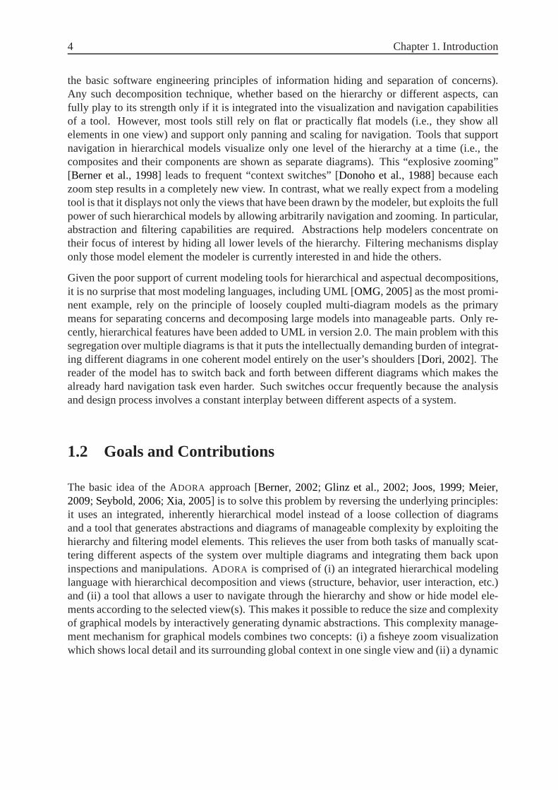
the basic software engineering principles of information hiding and separation of concerns).Any such decomposition technique, whether based on the hierarchy or different aspects, canfully play to its strength only if it is integrated into the visualization and navigation capabilitiesof a tool. However, most tools still rely on flat or practically flat models (i.e., they show allelements in one view) and support only panning and scaling for navigation. Tools that supportnavigation in hierarchical models visualize only one levelof the hierarchy at a time (i.e., thecomposites and their components are shown as separate diagrams). This “explosive zooming”[Berner et al., 1998] leads to frequent “context switches” [Donoho et al., 1988] because eachzoom step results in a completely new view. In contrast, whatwe really expect from a modelingtool is that it displays not only the views that have been drawn by the modeler, but exploits the fullpower of such hierarchical models by allowing arbitrarily navigation and zooming. In particular,abstraction and filtering capabilities are required. Abstractions help modelers concentrate ontheir focus of interest by hiding all lower levels of the hierarchy. Filtering mechanisms displayonly those model element the modeler is currently interested in and hide the others.
Given the poor support of current modeling tools for hierarchical and aspectual decompositions,it is no surprise that most modeling languages, including UML [OMG, 2005] as the most promi-nent example, rely on the principle of loosely coupled multi-diagram models as the primarymeans for separating concerns and decomposing large modelsinto manageable parts. Only re-cently, hierarchical features have been added to UML in version 2.0. The main problem with thissegregation over multiple diagrams is that it puts the intellectually demanding burden of integrat-ing different diagrams in one coherent model entirely on theuser’s shoulders [Dori, 2002]. Thereader of the model has to switch back and forth between different diagrams which makes thealready hard navigation task even harder. Such switches occur frequently because the analysisand design process involves a constant interplay between different aspects of a system.
1.2 Goals and Contributions
The basic idea of the ADORA approach [Berner, 2002; Glinz et al., 2002; Joos, 1999; Meier,2009; Seybold, 2006; Xia, 2005] is to solve this problem by reversing the underlying principles:it uses an integrated, inherently hierarchical model instead of a loose collection of diagramsand a tool that generates abstractions and diagrams of manageable complexity by exploiting thehierarchy and filtering model elements. This relieves the user from both tasks of manually scat-tering different aspects of the system over multiple diagrams and integrating them back uponinspections and manipulations. ADORA is comprised of (i) an integrated hierarchical modelinglanguage with hierarchical decomposition and views (structure, behavior, user interaction, etc.)and (ii) a tool that allows a user to navigate through the hierarchy and show or hide model ele-ments according to the selected view(s). This makes it possible to reduce the size and complexityof graphical models by interactively generating dynamic abstractions. This complexity manage-ment mechanism for graphical models combines two concepts:(i) a fisheye zoom visualizationwhich shows local detail and its surrounding global contextin one single view and (ii) a dynamic
1.2 Goals and Contributions 5
generation of different views on the model by filtering specific model elements. The view gen-eration mechanism facilitates the integration of multiplesystem aspects in one coherent modelwhile keeping the size and complexity of the resulting diagram within reasonable limits.
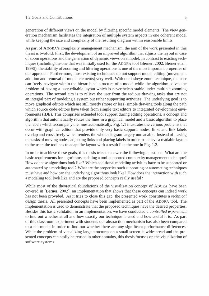
As part of ADORA’s complexity management mechanism, the aim of the work presented in thisthesis is twofold. First, the development of an improved algorithm that adjusts the layout in caseof zoom operations and the generation of dynamic views on a model. In contrast to existing tech-niques (including the one that was initially used for the ADORA tool [Berner, 2002; Berner et al.,1998]), the stability of zooming and filtering operations is one of the most important properties ofour approach. Furthermore, most existing techniques do notsupport model editing (movement,addition and removal of model elements) very well. With our fisheye zoom technique, the usercan freely navigate within the hierarchical structure of a model while the algorithm solves theproblem of having a user-editable layout which is nevertheless stable under multiple zoomingoperations. The second aim is to relieve the user from the tedious drawing tasks that are notan integral part of modeling a system but rather supporting activities. The underlying goal is tomove graphical editors which are still mostly (more or less)simple drawing tools along the pathwhich source code editors have taken from simple text editors to integrated development envi-ronments (IDE). This comprises extended tool support during editing operations, a concept andalgorithm that automatically routes the lines in a graphical model and a basic algorithm to placethe labels which accompany the lines automatically. Fig.1.1illustrates the various problems thatoccur with graphical editors that provide only very basic support: nodes, links and link labelsoverlap and cross freely which renders the whole diagram largely unreadable. Instead of leavingthe tasks of moving nodes, adjusting links and placing labels in order to achieve a readable layoutto the user, the tool has to adapt the layout with a result likethe one in Fig.1.2.
In order to achieve these goals, this thesis tries to answer the following questions: What are thebasic requirements for algorithms enabling a tool-supported complexity management technique?How do these algorithms look like? Which additional modeling activities have to be supported orautomated by a modeling tool? What are the properties such supporting or automating techniquesmust have and how can the underlying algorithms look like? How does the interaction with sucha modeling tool look like and are the proposed concepts really useful?
While most of the theoretical foundations of the visualization concept of ADORA have beencovered in [Berner, 2002], an implementation that shows that these concepts can indeed workhas not been provided. As it tries to close this gap, the presented work constitutes atechnicaldesignthesis. All presented concepts have been implemented as part of the ADORA tool. Theimplementation is used to demonstrate that the proposed techniques have the desired properties.Besides this basic validation in an implementation, we haveconducted acontrolled experimentto find out whether at all and how exactly our technique is usedand how useful it is. As partof this classroom experiment with students our abstractionmechanism has also been comparedto a flat model in order to find out whether there are any significant performance differences.While the problem of visualizing large structures on a smallscreen is widespread and the pre-sented concepts can easily be reused in other domains, this thesis focuses on the visualization ofsoftware systems.

6 Chapter 1. Introduction
readyForNextRequest
idle
movingDown
carDecelerating
movingUp
doorsClosed
doorsClosing
CarController
| send getNext() over manager
[floor == currentFloor] receive
request(floor) over cabin | send open()
over controlDoor
[currentFloor == requestedFloor] receive triggered() over limit
| send stop() over controlMotor; send open() over controlDoor
[floor != currentFloor] receive request(floor) over cabin | requestedFloor = floor;
send close() over controlDoor[currentFloor == requestedFloor] receive triggered() over slow
Down() | send reduce() over controlMotor
[currentFloor > requestedFloor] | send down() over control
Motor [currentFloor == requestedFloor] receive
triggered() over slowDown | send reduce() over
controlMotor
[currentFloor < requestedFloor] | send up() over controlMotor
receive closed() over doorState() |
Figure 1.1: Typical layout problems resulting from only rudimentary tool support
1.3 Thesis Outline
The thesis is split into several parts. The remainder of the introductory part first sketches inChapter2 the modeling field in general and its role in the software engineering discipline. InChapter3 the arising problems with the size and complexity of models of software systems andtechniques to mitigate them are discussed. Chapter4 introduces the modeling language ADORA
and shows its way to deal with the complexity and size of models. While most of the concepts ofthis thesis are presented independently of any specific modeling language (with the rudimentarynotation of nested node-link diagrams as the only requisite), the ADORA chapter shows their usewithin the context of a specific language.
Our own approach to cope with the complexity and size of graphical models is the topic of thesecond part. The first half of it comprises fisheye zoom techniques that can be used to showboth local detail and global context and different levels ofdetail. The properties such a fisheyezoom technique must have in order to be usable for iteratively created and maintained diagramsare introduced in Chapter5. Existing fisheye zoom techniques are then discussed with a specificemphasis on this properties in Chapter6. In Chapter7 our fisheye zoom algorithm is presented indetail. Chapter8 shows how the presented zoom algorithm can be used to dynamically generate

1.3 Thesis Outline 7
readyForNextRequest
idle
movingDown
carDecelerating
movingUp
doorsClosed
doorsClosing
CarController
| send getNext() over manager
[currentFloor > requestedFloor] |
send down() over controlMotor
[currentFloor == requested
Floor] receive triggered()
over slowDown | send
reduce() over controlMotor
[currentFloor < requestedFloor] |
send up() over controlMotorreceive closed() over doorState() |
[currentFloor == requestedFloor] receive triggered() over slow
Down() | send reduce() over controlMotor
[currentFloor == requestedFloor] receive triggered() over limit | send stop() over controlMotor; send open() over controlDoor
[floor != currentFloor] receive request(floor) over cabin | requestedFloor = floor;
send close() over controlDoor
[floor == current
Floor] receive
request(floor) over
cabin | send open()
over controlDoor
Figure 1.2: Enhanced tool support to automate layouting tasks
different views on the model by filtering specific model elements. While the previous chapterwere all concerned with the complexity and size of graphicalmodels, Chapter9 presents anextension of our zoom algorithm to support the user during model editing. Finally, Chapter10discusses the presented zoom algorithm in detail. This discussion spans an evaluation against thedesired properties and an assessment of the runtime and space complexity of the algorithm.
The dynamic layout that results from the application of our zoom algorithm has a big impact onthe links which connect the nodes in the diagram. These linksor lines are the topic of the thirdpart. Chapter11sets the stage by discussing the quirks of lines in hierarchal models whose layoutchanges continuously. Furthermore, the requirements for an automatic line routing algorithmthat works on such layouts are presented. A short overview ofexisting automatic line routingtechniques follows in Chapter12. Our own automatic line routing technique is introduced anddiscussed in Chapter13. The second part closes with a presentation of an automatic line labelplacement algorithm that is built upon the line router’s data structure in Chapter14.
Part four covers the constructive and empirical validationof the presented work in Chapters15and 16 respectively. The conclusions and an outlook on possible future work in Chapter17constitute the fifth part. The last part contains the Appendix with details about the experimentalvalidation.


9
CHAPTER 2
Graphical Modeling
Models and especially those that employ a graphical notation play an important role in the spec-ification and design of software systems. This chapter givesfirst an overview over the use ofmodels in general and the corresponding terminology with a special focus on graphical models.The role such models play in the software engineering field isoutlined in Section2.2. Subse-quently, Section2.3covers the assistance computer-based tools can offer in constructing, refiningand examining models. And finally, the last two sections discuss psychological aspects of graph-ical models, namely the role of aesthetics as well as the concepts of secondary notation andmental map.
2.1 Models and Their Representation
The ability to model allows us to interact with a complex world by reducing the vast flow ofinformation we constantly have to cope with. Using models makes it possible to deal with someclasses of problems rather than with a possibly unlimited number of individual problems. Thefact that models are usually not related to an individual object or phenomena but to a classthereof (i.e., the classification abstraction) makes them an extremely powerful tool. For example,the realization that a certain class of animals rather than one single individual is dangerous hasimproved the humans’ chance for survival significantly. Thus, models are an essential part ofour everyday life. We use them - often unconsciously - to think about problems, to talk to eachother, to understand phenomena and to teach. In contrast to this unconscious use of models, theirconstruction and analysis is an explicit topic in research and engineering. Research results in

10 Chapter 2. Graphical Modeling
theories, which are a special kind of models, that are highlyabstract and emphasize results andconclusions over obviousness. Models in engineering help in developing and understanding arti-facts by providing information about the consequences of building them before they are actuallymade [Ludewig, 2003].
Any artifact has, according toStachowiak[1973], to meet the following three criteria in orderto qualify as a model: (i) themapping criterionstates that there has to be an original object(which is called the “original”) or phenomenon that is mapped to the model, (ii) according to thereduction criterion, only some of the properties of the original are mapped to themodel and (iii)the model replaces the original for some purpose to be usefulwhich is stated by thepragmaticcriterion. Models that are not built of concrete material are expressed in a language. Thislanguage consists of a set of textual and/or graphical symbols (the so-callednotation) and theconceptual associations thereof. The rules of how to combine the symbols into valid structuresare defined by thesyntaxwhile thesemanticsdefine their conceptual meaning.
2.1.1 Graphical Representations
Graphical or visual models, which employ graphical symbolsas notation, occupy a central po-sition among the different kinds of models. The saying “a picture is worth a thousand words”stands for the widely accepted argument that graphical representations are universally superiorto text or any other non-graphical representation. Psychological theories explain the appeal ofgraphical representations with the finding that relativelylarge sections of static pictures or dia-grams can - in contrast to the dynamic, temporally ordered nature of language - be understoodin parallel. Therefore, it is possible to comprehend a complex visual structure in a fraction of asecond, based on a single glance [Ware, 2004]. However, the explicit distinction between paral-lel and sequential representations indicates that both graphics and non-graphical representationssuch as text have their uses and limitations and that none is inherently superior [Petre, 1995].
Another explanation for the attractiveness of graphical representations offers the theory of exter-nal cognition [Ware, 2004] which tries to explain how resources outside the mind can beusedto enhance the cognitive capabilities of the mind. Humans can interact with a rich and detailedworld because the world is “its own best model”. We do not needa detailed internal model of theworld because whenever we want to see detail we can get it by focusing attention on some aspector by moving our eyes to see the details in some other part of the visual field [Ware, 2004]. Thisprinciple can be exploited to solve many interesting problems that are too difficult or complex tobe solved purely mentally by using cognitive tools, such as pencils and paper and increasinglycomputer-based tools which makes it possible to substituteseeing for reasoning. The extent ofthis “computational offloading” to external tools is especially large in the case of graphical repre-sentations as they enable a picture of the whole problem to bemaintained simultaneously whileworking through the interrelated parts [Moody, 2009; Scaife and Rogers, 1996]. The emphasison interrelated parts in this explanation indicates that graphical representations are especiallypowerful for relational data.

2.1 Models and Their Representation 11
Graphical models and especially their underlying theoriesof cognition have gained a lot of atten-tion during the last years due to the development of information visualization (see e.g. [Spence,2007; Ware, 2004]) as a research field of its own. The principal task of information visualizationis to facilitate the derivation of information from data by supporting the beholder in forming amental map or image of something. Information visualization owes much of its success to therecent progress of computer graphics and the fact that visual displays provide the channel withthe highest bandwidth between the computer and the human user (more information is actuallyacquired through vision than all the other senses combined [Ware, 2004]). While the term visu-alization depicts both the process of graphically representing existing data and the result thereof,we use the term graphical modeling for the process of creating a graphical representation ofsomething. The result of this process is a graphical model, which is usually subject to change(i.e., the process is incremental).
2.1.2 Graphical Models of Abstract Phenomena
Geometric abstractions that are used to represent inherently geometric phenomena or objects ina graphical model are a very powerful tool. The floor plan of a building helps both the architectand the client to communicate and understand their intentions. Thanks to the direct geometricmapping between model and reality, contradictions and omissions become obvious [Brooks,1987]. Scale drawings of mechanical parts and chip designs servethe same purpose. The directrelation between representation and physical reality is also the main reason why maps, whichresemble miniature pictorial representation of the physical world [Tufte, 1997], are so powerfuland common. But nevertheless, already the abstractions employed in maps makes it hard formany people to understand and interpret them correctly.
Many notations for graphical models of phenomena which do not have an obvious or natu-ral graphical representation derived from their physical form1 try to exploit the natural spatialand geographic ways of thinking to make abstract information more accessible [Perlin and Fox,1993]. Humans intuitively tend to organize information spatially during their everyday life. Forexample, we are used to create stacks of similar informationand place each stack at some con-venient or easy remembered location on the desk [Donelson, 1978]. This spatial organizationprinciple has also been adopted by the metaphor of the virtual desktop on the computer screen.The question is then how such graphical representations have to look like in order to tap into thehuman’s natural spatial way of thinking.
Three-Dimensional versus Two-Dimensional Representations
The fundamental issue in any representation is how to depicta world of three or more dimensionson the “two-dimensional flatlands of paper” [Tufte, 1997]. This raises the question of whether
1The abstract form of the information that has to be represented is also the main point that distinguishes infor-mation visualization from other fields such as scientific visualization or geovisualization [Spence, 2007].

12 Chapter 2. Graphical Modeling
to use two or three dimensional representations. Obviously, a 3D representation offers one moredimension that can be used by the visualization. However, according toGershon et al.[1998] wedo not always understand when 3D is more effective. Additionally, the results of an experimentby Huotari et al.[2004] indicate that 3D is not necessarily inherently better than2D in abstractdomains and that we should therefore be cautious in making such claims. Even the increasein usable space from a 2D to a 3D display is not such a big advantage, because what is finallyseen on the screen is a 2D projection of the 3D space. The fact that we can only see a 2Dprojection imposes a fundamental limitation that manifests itself in the fact that the usable spacerelates much more closely to the 2D size ofn2 than the full 3D space ofn3 since we cannot seethrough objects [Carpendale et al., 1997a]. Despite this, the experimental study of 3D networkvisualization byWare et al.[1993] revealed that the number of errors in detecting paths througha directed graph is substantially reduced if a 3D display method is used. However, this is onlyachieved if the user can rotate the structure in any direction which stresses more the importanceof direct interaction than that of a 3D representation itself. An additional problem in connectionwith the representation of software systems is that software is intangible, so that there is noobvious meaning of the third dimension (already the 2D spatial organization does not have adirect meaning).
2.1.3 Node-Link Diagrams
One of the most frequently used graphical representations is the node-link (or box and arrow)diagram. Such a diagram uses nodes to represent various kinds of entities and links to depictthe relationships between these entities. The basic graphical elements of node-link diagrams arerectangles, circles or polygons that represent nodes and connecting lines depicting the links. Inanalogy to the phonemes which are the smallest (atomic) elements in speech recognition fromwhich meaningful words are made, such basic graphical elements of a visual language are calledgraphemes [Fish and Störrle, 2007; Ware, 2004]. Graphemes are extracted by the early neuralmechanisms which are in effect while looking at a graphical representation and have therefore alarge influence on the perception of graphical models.
The appeal of node-link diagrams can be explained by the so-called Gestalt laws which are theresult of the first serious attempt to understand the mechanisms of pattern perception undertakenin 1912 by the German psychologists Max Westheimer, Kurt Koffka and Wolfgang Kohler [Kof-fka, 1935]. The two most important Gestalt laws in connection with node-link diagrams areclosure and connectedness [Ware, 2004]. The Gestalt law of closure states that a closed contourtends to be seen as an object and that there is a very strong perceptual tendency to divide regionsof space into “inside” and “outside” the contour. This also explains why Venn-Euler diagramsare such a powerful device for displaying the relationshipsbetween sets of data. The secondGestalt law that is fundamental for node-link diagrams, connectedness, is achieved by connect-ing different graphical objects by lines. Connectedness isa very strong way of expressing thatthere exists some relationship between these objects. However, it restricts the applicability ofnode-link diagrams to the representation of data that is, atleast partially, relational.

2.1 Models and Their Representation 13
The use of nodes and links to depict entities and relations does only partially answer the questionof how to represent abstract information graphically. The role or meaning of the (absolute orrelative) location and shape of the nodes remains unclear, as there is usually no natural layoutfor an abstract (relational) structure [Moody, 2009]. In contrast, maps express quantities visu-ally by location (i.e., two-dimensional addresses of latitude and longitude) and by areal extent(i.e., surface coverage) [Tufte, 1997]. Replacing the map’s natural spatial scales with abstractscales of measurement that are not based on geographic analogy but still easily accessible andunderstandable remains a big challenge. The meaning of suchgeometric relationships is usuallydefined by the domain that is modeled.
Terminology
The theoretical background of node-link diagrams is the graph theory (see e.g. [Gross and Yellen,1998]) which uses mathematical structures to model pairwise relations between objects. Thegraph theory has a widely accepted terminology: AgraphG in this context is an ordered paircontaining a set ofverticesV and a multiset ofedgesE:
G = 〈V,E〉 (2.1)
whereE contains unordered pairs of vertices which are not necessarily distinct, so that:
E ⊆ V × V (2.2)
Certain restrictions on the relations that are representedby the edges yield special classes ofgraphs that are of particular interest for certain applications. One the most frequently used typeof graphs in computer science is the tree [Knuth, 1997]. A tree is a graph in which any twovertices are connected by exactly one path. Apath in a graph is a sequence of vertices such thatfrom each of its vertices there is an edge to the next vertex inthe sequence. Alternatively, anyconnected graph with no cycles is a tree, where acycleis a path such that the start and end vertexare the same. Two verticesU andV areconnectedif the graph contains a path fromU to V .Consequently, a graph is connected if each pair of vertices in it is joined by a path. The specifictopological restrictions and the broad use of trees has produced a whole terminology specificallyfor trees. Each vertex in a tree has an edge to exactly oneparent, except for theroot, which hasno parent. Conversely, each vertex can have (i.e., be connected to) any number ofchildren. Ageneralization of the parent-child relationship is theancestor-descendantrelationship. Verticesthat have the same parent aresiblingsand a vertex that has no children is called aleaf. Thelevelof a vertex in a tree is a measure of its distance from the root and is defined as follows: (i) ifvertexX is the root of the tree, its level is1 and (ii) if vertexX is not the root, its level is1 + itsparent’s level. Theheightof a tree is the maximum level of any vertex in the tree. If a graph thathas no cycles is not connected (i.e., a disjoint union of trees), it is called aforest.

14 Chapter 2. Graphical Modeling
Basic graphs can only represent binary relations on a set of elements. Ahypergraphwhich isan extension of a basic graph can additionally express one-to-many relationships. An edge nolonger connects a pair of nodes, but rather a subset thereof.A hypergraphH is still an orderedpairH = 〈V,E〉 whereV is a set of vertices butE is now a set of non-empty subsets ofV calledhyperedges:
E = P(V ) \ ∅ (2.3)
whereP(V ) is the power set ofV . Hyperedges are arbitrary sets of nodes, and can thereforecontain an arbitrary number of nodes. Another extension to basic graphs that lies somewherein the middle between simple graphs and hypergraphs arenested graphs. The vertices of sucha nested (or hierarchically clustered) graph [Noik, 1994] can contain other vertices. A nestedgraphN is defined by
N = 〈V,E, C〉 (2.4)
whereC is a set of containment relations which are restricted to be hierarchical (i.e.,C is a treeor a forest of trees):
C ⊆ V × 2V (2.5)
The graphs as discussed so far are abstract, non-graphical structures. Adiagram2 or layout isa graphical representation of such a graph. Vertices are represented bynodesand edges aredepicted bylinks, which results in node-link diagrams. We use the terms node and link to dis-tinguish them from the abstract graph theoretical conceptsof vertex and edge. The one-to-manyrelations in hypergraphs are more difficult to draw and therefore tend to be studied using the ter-minology of set theory rather than the more pictorial descriptions of graph theory [Harel, 1988].Thus, graphical representations of hypergraphs typicallydraw from the Venn-Euler diagramsthat are used to represent set relationships. Similarly, the containment edges of nested graphs areoften displayed as boxes that fully enclose the nodes associated with the nested vertices.
2.2 Graphical Models in Software Engineering
Two of the main reasons why developing software is difficult are the complexity of the problemat hand and the intangible (or invisible) nature of the software itself [Brooks, 1987]. Modelsplay an important role in coping with these two problems and are therefore found in almost allareas and applications of software engineering3. We limit ourselves here to prescriptive system
2The terms diagram and graphical model are used interchangeably in this thesis.3We follow here the definition of theIEEE [1990] which defines software engineering as “the application of a
systematic, disciplined, quantifiable approach to the development, operation, and maintenance of software”.
2.2 Graphical Models in Software Engineering 15
models (i.e., formal or semi-formal models of computer-based systems) and do not considerprocess models or process maturity models.
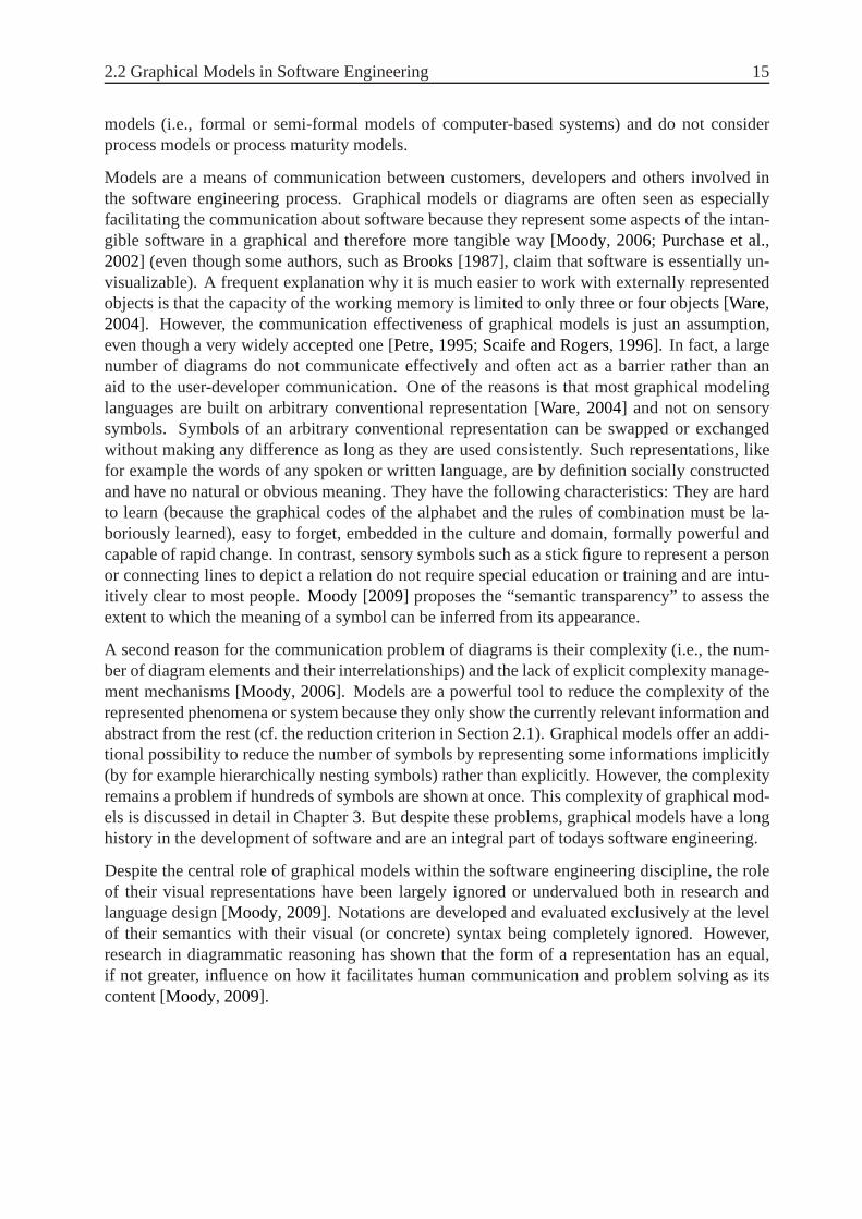
Models are a means of communication between customers, developers and others involved inthe software engineering process. Graphical models or diagrams are often seen as especiallyfacilitating the communication about software because they represent some aspects of the intan-gible software in a graphical and therefore more tangible way [Moody, 2006; Purchase et al.,2002] (even though some authors, such asBrooks[1987], claim that software is essentially un-visualizable). A frequent explanation why it is much easierto work with externally representedobjects is that the capacity of the working memory is limitedto only three or four objects [Ware,2004]. However, the communication effectiveness of graphical models is just an assumption,even though a very widely accepted one [Petre, 1995; Scaife and Rogers, 1996]. In fact, a largenumber of diagrams do not communicate effectively and oftenact as a barrier rather than anaid to the user-developer communication. One of the reasonsis that most graphical modelinglanguages are built on arbitrary conventional representation [Ware, 2004] and not on sensorysymbols. Symbols of an arbitrary conventional representation can be swapped or exchangedwithout making any difference as long as they are used consistently. Such representations, likefor example the words of any spoken or written language, are by definition socially constructedand have no natural or obvious meaning. They have the following characteristics: They are hardto learn (because the graphical codes of the alphabet and therules of combination must be la-boriously learned), easy to forget, embedded in the cultureand domain, formally powerful andcapable of rapid change. In contrast, sensory symbols such as a stick figure to represent a personor connecting lines to depict a relation do not require special education or training and are intu-itively clear to most people.Moody [2009] proposes the “semantic transparency” to assess theextent to which the meaning of a symbol can be inferred from its appearance.
A second reason for the communication problem of diagrams istheir complexity (i.e., the num-ber of diagram elements and their interrelationships) and the lack of explicit complexity manage-ment mechanisms [Moody, 2006]. Models are a powerful tool to reduce the complexity of therepresented phenomena or system because they only show the currently relevant information andabstract from the rest (cf. the reduction criterion in Section2.1). Graphical models offer an addi-tional possibility to reduce the number of symbols by representing some informations implicitly(by for example hierarchically nesting symbols) rather than explicitly. However, the complexityremains a problem if hundreds of symbols are shown at once. This complexity of graphical mod-els is discussed in detail in Chapter3. But despite these problems, graphical models have a longhistory in the development of software and are an integral part of todays software engineering.
Despite the central role of graphical models within the software engineering discipline, the roleof their visual representations have been largely ignored or undervalued both in research andlanguage design [Moody, 2009]. Notations are developed and evaluated exclusively at thelevelof their semantics with their visual (or concrete) syntax being completely ignored. However,research in diagrammatic reasoning has shown that the form of a representation has an equal,if not greater, influence on how it facilitates human communication and problem solving as itscontent [Moody, 2009].

16 Chapter 2. Graphical Modeling
2.2.1 A Short History of Graphical Modeling Languages
The popularity and importance of graphical models and especially node-link diagrams in soft-ware engineering is illustrated in the following by a short history of graphical modeling lan-guages (without any claim for completeness). The history ofgraphical modeling languages datesback to the beginning of computer sciences. Probably the first widely known graphical notationis theFlowchartwhich was developed by Herman Goldstine and John von Neumannat PrincetonUniversity in late 1946 and early 1947 [Goldstine and von Neumann, 1947]. This basic idea ofdocumenting process flow goes back to previous work in other fields such as industrial engineer-ing. A flowchart is a node-link diagram representing an algorithm or a process by showing thesteps as boxes of various kinds and their order of execution by directed links.
The focus of thePetri netnotation which was published by Carl Adam Petri in his doctoral thesis[Petri, 1962] lies on modeling the concurrent behavior of distributed systems (Petri invented thenotation years before its publication to describe chemicalprocesses). Petri nets have two kindsof alternating nodes, places and transitions, which are connected by directed links. Places maycontain any number of tokens and a transition may fire whenever there is a token at all places thathave a directed link to it; when it fires, it consumes these tokens, and places them at the placesit has a directed link to. In 1967, Taylor Booth [Booth, 1967] introduced thestate diagramtodescribe the behavior of a system. A state diagram describesthe possible states of a system orobject as events occur. States are represented by nodes and state transitions by the links betweenthese nodes.
TheNassi-Shneiderman diagramor Structogram was developed in 1972 by Isaac Nassi and BenShneiderman [Nassi and Shneiderman, 1973] as a graphical notation for the structured program-ming paradigm. Hence, it can be seen as the graphical answer to Edsger Dijkstra’s call for theabolishment of the GOTO statement from high-level languages in the interest of improving thequality of the code [Dijkstra, 1968]. Nassi-Shneiderman diagrams use nested boxes to representsubproblems (i.e., the structure is represented by the nesting and position of the boxes withoutthe need of any links). In contrast to Flowcharts which gained much of their popularity fromthe possibility to easily express GOTOs or jumps, such constructs can not be represented inNassi-Shneiderman diagrams. The notation was popular during the 80’s but is nowadays onlyrarely used because its abstraction level is too strongly tied to structured program code and mod-ifications usually require the whole diagram to be redrawn. The HIPO (Hierarchy plus Input-Process-Output) technique, developed by IBM in 1974 for planning and documenting computerprograms, consists of a hierarchy chart that graphically represents the program’s (hierarchical)control structure in a tree and a set of Input-Process-Output charts that describe the functionsperformed by each module on the hierarchy chart [IBM, 1974]. In 1975, Michael A. Jack-son published theJackson Structured Programming(JSP) method for structured programming[Jackson, 1975] that is based on the correspondences between data stream and program structure.Jackson’s method structures programs and data in terms of sequences, iterations and selectionsand represents the result graphically in a tree.
Peter Chen’sEntity-Relationship Model(ERM), published in 1976, directed the focus of sys-

2.2 Graphical Models in Software Engineering 17
tem modeling from processes and system behavior towards data [Chen, 1976]. Its conceptualdata model is represented in entity-relationship diagramswhich depict the entities, relationsand attributes as different kinds of nodes and connects themby links. In contrast to the entityrelationship models that target mainly data-driven information systems, theSpecification andDescription Language(SDL), first published in 1976 by the International TelecommunicationsUnion and continuously extended and adjusted over the time [ITU-T, 2000], is mainly used todescribe the behavior and structure of distributed, event-driven, real-time systems. The graph-ical representation of SDL (SDL/GR) consists of a hierarchyof different diagrams that followthe hierarchical decomposition of a system. The top level describes the system with a set ofblocks (nodes) that communicate over channels. Each of these blocks is specified by a set ofprocesses (nodes) and connecting signal routes (links) in adiagram of its own. On the next lowerlevel, a process is described by an extended finite state machine. The procedures of this statemachine can be further divided into a set of procedure diagrams. SDL originally focused ontelecommunication systems, but is currently used in additional areas including process controland real-time applications in general. The language has formal semantics, so that it can be usedfor code generation and simulation.
The term “structured” was the buzzword of the second half of the seventies. In 1975, EdwardYourdon and Larry L. Constantine published theirStructured Design(SD) method [Yourdonand Constantine, 1975] that uses so-called structure charts as graphical notation to describe therelations (links) between modules (nodes). Roughly at the same time, Douglas T. Ross developedin 1976/77 theStructured Analysis and Design Technique(SADT) [Ross and Schoman, 1977]which uses two types of diagrams, activity models and data models. SADT offers building blocks(nodes) to represent entities and activities, and a varietyof arrows to relate these boxes by links.Blocks can be decomposed in a top-down approach so that each block is described in a diagramof its own. The different kinds of relations (links) are distinguished by the side they enter orleave a block. Finally, Tom DeMarco’sStructured Analysis(SA) [DeMarco, 1979] uses dataflowdiagrams (DFD) to describe a system. A dataflow diagram consists of the nodes activity (orprocess), store and terminal that are connected by links, which represent the flow of data. Eachactivity can be described in a dataflow diagram of its own which results in a DFD hierarchy.
Two of the biggest problems of state diagrams, the combinatorial explosion of the number ofstates in models with a lot of parallelism and the lack of the possibility to hierarchically decom-pose large models, have been addressed in 1987 by theStatechartnotation of David Harel [Harel,1987]. In addition to state diagrams, the statechart notation allows the modeling of superstates,concurrent states, and activities as part of a state. A statein a Statechart can either be elementary,hierarchically decomposed into another Statechart or intomultiple parallel statecharts. Whilethe original finite state machines are disjunctive (i.e., the machine can only be in one of all thepossible states at once), a Statechart can be in two or more states concurrently.
The abundance of methods and notations that came along with the next paradigm shift to theobject-oriented software development at the beginning of the 1990s resulted in the call for ashared graphical language of description and specification. Such a communication medium forboth humans and software tools has been a central part of other, admittedly more mature, engi-

18 Chapter 2. Graphical Modeling
neering disciplines such as civil or mechanical engineering for decades. The answer of three ofthe more prominent methodologists of these years was theUnified Modeling Languagewhichwas published as first draft in 1996.
2.2.2 The Unified Modeling Language
The Unified Modeling Language (UML) was the byproduct of the failed attempt by the “ThreeAmigos” James Rumbaugh, Ivar Jacobson and Grady Booch to agree upon a uniform methodfor object-oriented software development. UML 1.1 has beenaccepted as the standard modelinglanguage by the industry consortium Object Management Group (OMG) in 1997. Thereafter,the OMG has supervised its development and has been astonishing successful in establishingUML as the de-facto industry standard for the object-oriented modeling of software systems.After several minor revisions (UML 1.2, 1.3, 1.4 and 1.5) to fix shortcomings and bugs, a majorrevision resulted in version 2.0 [OMG, 2005] on which the following discussion is based. UMLprovides a collection of several more or less loosely coupled graphical notations that facilitatethe construction of requirements and design models. The language employs thirteen (node-link)diagrams to represent eight different views on the system. As shown in Fig.2.1the diagrams aredivided into three categories (indicated by the names in italics in Fig.2.1).
UML-Diagram
Structure
Diagram
Behaviour
Diagram
Class
Diagram
Component
Diagram
Object
Diagram
Use Case
Diagram
State Machine
Diagram
Activity
Diagram
Composite
Structure
Diagram
Deployment
Diagram
Package
Diagram
Interaction
Diagram
Sequence
Diagram
Interaction
Overview
Diagram
Communication
Diagram
Timing
Diagram
Figure 2.1: Hierarchy of UML 2.0 diagrams, represented as UML class diagram [OMG, 2005]
Six diagram types represent the static structure of the application, three general types of behavior,and the last four show different aspects of interaction. At the heart of the UML lies theclass

2.2 Graphical Models in Software Engineering 19
diagramthat specifies the static structure of the system by showing the system’s classes, theirattributes and methods together with the relationships between classes and among their instances.The remaining structure diagrams are the following: Acomponent diagramshows how a systemis split up into components and depicts the dependencies between these components. Anobjectdiagramshows a complete or partial view of the structure of the system at a specific momentin time. This snapshot focuses on some particular set of object instances and attributes, and thelinks between these instances. Thecomposite structure diagramshows the internal structure of aclass and the collaborations which can take place in this structure. Adeployment diagramcan beused to model how the system’s components are deployed on thehardware, and the associationsbetween the components. Finally, apackage diagramdepicts how a system is split up into logicalgroupings by showing the dependencies among these groupings. This very brief overview overthe structure diagrams of UML already indicates that the different diagrams and the underlyingconcepts overlap. Therefore, it is often difficult to clearly separate UML’s concepts from eachother.
The behavior diagrams emphasize the dynamic behavior of thesystem being modeled. Anactiv-ity diagramshows the overall flow of control similar to flowcharts but with the additional pos-sibility to model parallelism. The UMLstate machine diagramis essentially a Harel statechartwith standardized notation.Use case diagramspresent a graphical overview of the functional-ity of a system in terms of actors, their goals (represented as use cases), and some rudimentarydependencies between these use cases and actors. As a subsetof the behavior diagrams UMLcontains the following interaction diagrams that emphasize the flow of control and data betweendifferent entities of the system: Asequence diagramshows how a set of messages betweenentities are arranged in time sequence while atiming diagramis a a special form of such a se-quence diagram with the focus on timing constraints.Interaction overview diagramsare a kind ofactivity diagram in which the activities are fragments of sequence diagrams. And finally, acom-munication diagramshows, similarly to a sequence diagram, the interactions between objects orparts. Unlike a sequence diagram, a communication diagram explicitly shows the relationshipsbetween elements but does not represent the time as a separate dimension.
UML has met with a lot of criticism over the years of its existence. The language is frequentlycriticized for the complexity and size of its notation (see e.g. [Dori, 2002]). The UML 2.0superstructure standard and its complementing infrastructure standard span together more than900 pages. The language contains, as already visible in the above description, many diagramsand constructs that are often redundant. Additionally, a lot of the constructs are rarely used inpractice. The size and complexity of UML impedes its understandability as empirical evidence[Nordbotten and Crosby, 1999] indicates that notations with a simpler graphic syntax areeasierto interpret. Because of its large number of symbols and keywords, UML often looks as compli-cated as a full programing language even though it claims to be accessible to a broader audiencethan any programing language. Another problem concerning the graphical notation of UML isthat a lot of its symbols are overloaded [Fish and Störrle, 2007]: The same grapheme (cf. Section2.1.2) is often used for two or more different concepts (e.g., the white or empty diamond in UMLrepresents a decision/merge in activity diagrams, but alsoan aggregation in class diagrams). This
20 Chapter 2. Graphical Modeling
overloading is used to reduce the number of graphemes in the language but it hinders the under-standability and learnability as the context (e.g., the current diagram) has additionally to be takeninto account to resolve the arising ambiguity.
UML has also often been criticized for the lack of possibilities to hierarchically decomposemodels so that it can also be used to describe large and complex systems (see e.g. [Glinz et al.,2002; Kobryn, 2004]). It owes this deficiency to the entity-relationship notation [Chen, 1976]from which UML (like most of the object-oriented modeling notations) has evolved and whichdoes not know a hierarchical decomposition either. The situation has improved with the re-lease of UML 2.0 which allows a hierarchical decomposition of some structural and behavioralconstructs. Such hierarchical decompositions of graphical models to manage their increasingcomplexity is discussed in detail in Section3.3. Another area of concern is the often unclear ormissing semantic definition of language constructs in the standard [Glinz, 2000]. In contrast toany formally defined programming language, UML is more an informally defined set of conven-tions that are used in different ways appropriate for the current problem at hand.
2.2.3 Graphical Programming and Model-Driven Engineering
The idea of applying graphical models not complementary to textual programming languagesbut using them exclusively to program graphically has risenup for the first time in the 1980s aspart of the effort summarized by the then buzzword of “computer-aided software engineering”(CASE). The focus of CASE was on developing methods and toolsthat enabled software devel-opers to express their designs in terms of general-purpose graphical programing representationssuch as state machines or flowcharts. But apart from a few specific domains such as the Matlab,Simulink, Stateflow stack in the automotive and avionics field, graphical programming had rela-tively little impact on the commercial software development. The aim of graphical programingwas, like of any new software development paradigm, to take the developer further away fromthe machine details by raising the level of abstraction. A raise in the level of abstraction is theusual answer to a “software crisis” which regularly emergesas soon as the current paradigm ofprogramming is no longer sufficient to handle the complexityof the problems developers areasked to solve [Riel, 1996]. However, most graphical programing languages do not increase thelevel of abstraction but employ just a different representation of computer programs than textualprograming languages.
In fact, graphical representations of computer programs are often harder to understand and main-tain than the equivalent representation in a high-level textual programming language. This is dueto the fact that many of the cognitive operations that are required for current (sequential) pro-gramming have more in common with processing natural language than with visual processing.The source code of computer programs is actually a linear (one-dimensional) data type [Shneider-man, 1996]. Ware[2004, p. 302] attributes the failure of flowcharts to their lack ofcommonalitywith natural language (even though the lack of structure mayhave been as important [Brooks,1995]). The parallel nature of our visual system explains also why graphical representations are
2.3 Tool Support for the Modeling Process 21
more frequently used to depict structural informations rather than dynamic (sequential) informa-tion such as processes or flows. As a consequence, textual andgraphical representations haveboth their advantages and disadvantages [Petre, 1995]. Thus, hybrid approaches that take thebest of both worlds by presenting and manipulating structure graphically (e.g., by representingmodules as nodes connected by links) and the detailed procedures or methods using text are oftenmore effective.
The idea of replacing textual programming languages with mostly graphical models has againgained a lot of popularity recently due to the advent of the so-called “model-driven engineer-ing” (MDE) (see e.g. [Schmidt, 2006]). MDE spans a set of different software developmentapproaches that use models as the primary form of expression. The focus on models is meantto avoid the problem of the current use of models in which diagrams are rarely in sync with theimplementation during later stages of a project. Contrary to previous attempts, MDE emphasizesthe use of domain specific modeling languages (DSML) insteadof general-purpose notations.The focus on domain specific languages stems from the observation that especially visual lan-guages are inherently domain specific and that an attempt to move beyond the domain levelabstraction results in large and complex visual structuresthat are impossible to comprehend (asshown by the history of flowcharts or UML). The MDE proponentsclaim that the use of domainspecific languages together with (the other buzzwords of) reusable class libraries, applicationframeworks and middleware platforms raises the level of abstraction available to software devel-opers. As with any new approach that claims to reduce the complexity by an order-of-magnitude,the question remains whether the approach does not abstractaway the essence of the softwarewhile trying to reduce its complexity (which is often achieved by simply decreasing its expres-siveness) since the complexity is an inherent property of software [Brooks, 1987].
The currently best known MDE initiative is the Model-DrivenArchitecture (MDA) of the ObjectManagement Group [OMG, 2003]. The MDA approach separates the specification of a system’sfunctionality from the specification of the implementationof that functionality on a specifictechnology platform. The result of this separation are platform independent models (PIM) andplatform specific models (PSM). Transformations between these models should, at least partially,be automated. The PIMs and PSMs are both intended to be expressed in OMG’s Unified Mod-eling Language (cf. Section2.2.2), using its profile and stereotype mechanisms to specializeandextend the language for different contexts.
2.3 Tool Support for the Modeling Process
The process of creating a graphical model of a software system is highly iterative as the modelis build incrementally step by step in collaboration with different stakeholders. Computer-basedtools are especially well suited to deal with changes and refinements that occur frequently in iter-ative processes. They make it easy to store, change and shareelectronic models. Most of the pastand current modeling tools provide exactly these basic functionalities. These tools are essen-tially drawing programs that employ a palette consisting ofthe specific symbols that constitute

22 Chapter 2. Graphical Modeling
the notation of the language and enforce some of the basic constraints of its syntax. However,computer-based tools can do a lot more than just replace the paper with a screen and the penwith a mouse, especially if they exploit the inherent structure and semantics of graphical models.The possibility to directly interact with the presented information is the principal feature thatseparates modern computer-based tools from paper based solutions [Spence, 2007]. Objects onthe screen should be active and not just a blob of color, so that they are capable of displayingmore information as needed, disappearing when not needed, and accepting user commands tohelp with the thinking process [Ware, 2004]. Unfortunately, the support to interact with a modelby exploiting its structure and semantics is rather limitedin todays graphical modeling tools. Thebest one can hope for are the very basic semantics of node-link diagrams which are supported inso far that links move with the nodes they connect.
Computer-based tools can ease the work with graphical models but they also employ specificproblems that do not occur if models are drawn on paper. Computer screens are getting biggerbut are still quite small and have a poor resolution comparedto the one that is possible on pa-per. Additionally, a computer screen is often filled with scroll bars, tool bars and other computeradministration stuff that is not needed on paper. Accordingto Hornbæk and Frøkjær[2003],the following problems occur while reading electronic (text) documents: a cumbersome navi-gation, lack of overview of the document, lower tangibilityof electronic documents comparedto paper, unclear awareness of the length of the documents, lower reading speed caused by thepoor resolution of most screens and fatigue if reading for extended periods of time. Thus, paperand computer-based tools are complementary: computers aregood at selecting, organizing andcustomizing information while paper makes the high-resolution information visible in portable,tangible and permanent form [Tufte, 1997].
2.3.1 Automatic Graph Drawing Algorithms
While computer-based modeling tools offer only moderate assistance for the creation and mod-ification of graphical models, automation plays a much bigger role in the automatic drawingof abstract graph structures as diagrams. Automatic graph drawing algorithms take a relationalgraph structure as input and produce a diagram (i.e., they define the layout of the diagram) tovisualize the information embodied in the graph. A multitude of such algorithms have beendeveloped (see [Battista et al., 1994] for an overview). The metrics to measure the quality ofthese algorithms are the degree to which they optimize certain aesthetics (e.g., minimal numberof link crossings, maximal symmetry or minimal number of bends in links) which should helpthe human reader to understand the information embodied in the graph and the algorithm’s com-putational efficiency. In the software engineering field, automatic graph drawing algorithms arewidely used by reengineering tools to visualize the static structure of existing software systems.
Applying automatic graph drawing algorithms in a specific domain, such as the visualization ofthe structure of a software system, entails two main problems. First, algorithms that are designedfor abstract graph structures do not necessarily produce useful visualizations of semantic infor-

2.3 Tool Support for the Modeling Process 23
mation because they cannot take the semantics of the domain the graph is used in into account.But, exactly this meaning of the nodes and links is the most important criterion for the layout.A good layout is to a large extent based on high level semantics which cannot be formalizedat present so that they cannot be employed in a graph drawing algorithm [Ware et al., 1993].Those conventions and common sense that can be formalized have to be coded explicitly intothe algorithm. For example, reengineering tools often produce UML class diagrams of parts of asoftware system to show the system’s structure. Class diagrams are usually drawn with the con-vention that a superclass is drawn above its subclasses. This simple convention is already quitehard to achieve with an automatic graph drawing algorithm. The second big problem is that theuser has usually no or only very little influence on the layoutthat is produced by an automaticgraph drawing algorithm. The layout is completely defined bythe algorithm and it is impossiblefor the user to adapt the layout to his personal preferences.
2.3.2 Layout Creation and Layout Adjustment
An important distinction between domains that employ automatic graph drawing algorithms andthe manual incremental creation of graphical models is the process that yields the diagram. Auto-matic layout algorithms take an abstract structure as inputand produce, in one step (i.e., in batchmode), a layout for the entire graph. Small changes in the abstract structure (e.g., the additionor removal of just one link) can have a tremendous influence onthe resulting layout because thelayout is calculated from scratch after every change. Hence, automatic graph drawing algorithmscannot be used for incremental layouts because the diagram is totally rearranged each time theuser changes something. In contrast to the graph drawing domain, the graphical modeling do-main is not dealing with the creation of a complete layout from an abstract representation, butwith the adaption of an existing layout to relatively minor changes. Thus, the goal is not a glob-ally optimal layout starting from a randomly chosen initialsetup, but instead to find the nearestlocal optimum starting from a relatively good initial position [Misue et al., 1995].
Misue et al.[1995] distinguish between “layout creation” and “layout adjustment” for the twodifferent modes to produce a diagram. Layout creation is thecalculation of a layout for an ab-stract structure in one step. In the layout adjustment mode,changes are constantly made. Alayout that has been spoiled in a local manner by such a changehas to be adjusted accordinglywithout totally rearranging the overall layout.Freire and Rodríguez[2006] use the terms “fixed”and “incremental” layout, whileMiriyala et al. [1993] distinguish between a “static” and “dy-namic” mode of automatic graph drawing.Bridgeman and Tamassia[2000] go one step furtherby distinguishing between “incremental graph drawing” where nodes are added one at a time andthe more general case of “interactive graph drawing”, in which any combination of node/link in-sertion and removal is allowed at each step.

24 Chapter 2. Graphical Modeling
2.4 Aesthetics in Diagrams
Even though the automatic graph drawing algorithms can usually not be used directly by a mod-eling tool, they raise with their attempt to optimize certain aesthetic criteria the question aboutthe role of aesthetics in graphical models. These aesthetics play also an important role for othertasks beside the automatic layout. For example, the best wayto route the links in a node-linkdiagram is largely defined by the underlying aesthetic criteria. The graph drawing literature listsa large number of aesthetics which an algorithm should optimize to help the human reader in un-derstanding the information embodied in the underlying graph structure (see e.g. [Tamassia et al.,1988] for general graphs or [Sindre et al., 1993] for nested graphs). However, there has been lit-tle attempt to use empirical methods to determine whether graphs that are laid out according tospecific aesthetic principles are in fact easier to understand.
Two exceptions are the work byWare et al.[2002], which provides empirical support for theclaim that the number of bends in a link and the number of link crossings degrade performanceon the task of finding the shortest path between two nodes, andthe experiment byPurchase et al.[2002] to investigate the merit of automatic graph layout algorithms with respect to human use.As part of their experiment, Helen Purchase and her colleagues measured the effect of individualaesthetics on human performance (i.e., response time for each question and the correctness ofthe answer) with respect to the ability of subjects to answerquestions about the structure of anabstract graph. The questions were chosen so that they measure only the understandability ofthe semantics of a node-link diagrams (i.e., the concept of nodes that are connected by links)independently of a specific domain. Example questions were the length of the shortest pathbetween two given nodes or the number of nodes that have to be removed from a graph in orderto disconnect two given nodes completely. The five investigated aesthetics were: (i) minimizingthe totalnumber of bendsin the links, (ii) minimize thenumber of link crossingsin the diagram,(iii) maximize theangle between linksextending from a node, (iv) maximize theorthogonalityby fixing the nodes and links on an orthogonal grid and (v) displaying asymmetrical viewof thegraph if possible. The result of the experiment with 55 individuals indicated support for reducingthe number of links crossings and bends in the links, and increasing the display of symmetry. Nosupport was found for maximizing the minimum angle or increasing orthogonality.
A second set of experiments aimed to investigate how the semantic domain of the graph drawingsaffects which aesthetic criteria need to be emphasized. UMLclass and collaboration diagramswhere used as the semantic domain. The users’ preference wasused as the method of usabil-ity measurement in these experiments. The experiments resulted in the following priority orderof aesthetics for both UML class and collaboration diagrams: (1) minimize the number of edgecrossings, (2) maximize orthogonality, (3) explicitly indicate the direction of information flow onthe links, (4) minimize the number of bends in the links, (5) use only horizontally aligned labels,(6) minimize the physical width of the layout and (7) employ only one font type for labels ratherthan using different fonts for different types of labels. This priority order of aesthetics suggeststhat the semantic domain of the graph drawings affects the aesthetic criteria that should be em-phasized. For example, the orthogonality of the drawing wasnot a significant aesthetic criteria

2.5 Secondary Notation and Mental Map 25
for abstract graphs but seems to be important for UML class and collaboration diagrams. Thisis a clear sign that algorithms that are designed for abstract graph structures will not necessarilyproduce useful visualizations of semantic information. Additionally, the experiments revealedthe difficulties to exclude confounding factors from the study. The aesthetic features that wereinvestigated have been selected from a large set (see e.g., [Coleman and Parker, 1996]). Outof these, the direction of information flow has not been targeted as an aesthetic feature in thebeginning but had to be added later in order to explain some unexpected results.
2.5 Secondary Notation and Mental Map
The difficulties in drawing diagrams automatically do not only stem from the neglect of thesemantics of the modeling language but also from layout cuesthat are often used in diagrams toexhibit structures and relationships. These cues are typically not formally part of the languagedefinition, but belong to a so-called “secondary notation” [Petre, 1995]. This secondary notationuses layout and perceptual cues (e.g., clustering, white space, relative or absolute position and/orsize) to clarify information or give hints to the reader.Fish and Störrle[2007] use the term“pragmatics” (or implicature) for this information that can be obtained from the diagram, butwas not encapsulated in the semantics or in the abstract model. The layout conventions of thesecondary notation are usually developed by experts in order to convey more information thanis actually contained in the abstract model. Such conventions are rarely formalized or codifiedwhich makes it hard or impossible to employ them in an automatic graph drawing algorithm.Examples in the software domain are the convention to draw a superclass above its subclasses inUML class diagrams (i.e., the inheritance relation is usually drawn bottom-up) or the placementof the nodes in UML activity diagrams so that the flow is from top to bottom or left to right.
The use of the secondary notation is, like good design, subject to personal style and individualskills [Petre, 1995]. Poor use of secondary notation which usually distinguishes diagrams drawnby novices from those drawn by experts makes representations more difficult to comprehend.Novices often fail to exploit the available layout cues (i.e., by dispersing related nodes) or evenintroduce mis-cues by for example using the Gestalt laws of symmetry or proximity arbitrarilyso that the (experienced) reader draws incorrect conclusions. The secondary notation plays alsoan important role in the differences in strategies that are employed to read diagrams [Petre,1995]. Readers have to identify and learn inspection strategiesfor diagrams which are processedand understood in parallel [Ware, 2004] and are therefore not amenable to the straight, serialreading style of text documents (see e.g. [Hornbæk and Frøkjær, 2003] for a discussion of readingpatterns). The cues that can be used to navigate a diagram areusually part of the secondarynotation. For example, the grouping or clustering of nodes can be exploited to reduce the searchspace and focus on that part of the diagram that contains the relevant information [Petre, 1995].
While the layout of a diagram is used by the secondary notation to add additional information,the geometric structure of the diagram also plays an important role in how the user interacts witha diagram over time. The user builds a strong “geographic” model [Bartram et al., 1995] in his

26 Chapter 2. Graphical Modeling
mind that is represented in the so-called “mental map” [Eades et al., 1991; Misue et al., 1995].Users construct this mental map of the visualized information structure in order to effectivelynavigate and search for information [Huotari et al., 2004]. The mental map allows the user toreduce the space he has to search for a specific node or link. The empirical finding that visualrecognition is a lot faster and more efficient than visual recall [Ware, 2004] indicates that themental map is not an exact image of the diagram in the user’s head but rather a representation ofits overall shape. Some formal measurements for the mental map and a discussion of the criteriathat have to be fulfilled in order to preserve it are discussedin Section5.3.

27
CHAPTER 3
Complexity of Graphical Models
Complexity is probably the single most important challengethe software engineering disciplinefaces today. The elements of a software system interact witheach other in a nonlinear fashion, sothat the complexity of the whole increases much more than linearly with the number of elements[Brooks, 1987]. The essential complexity of software systems stems largely from the complexityof the problem that has to be solved and the environment the system is embedded in [Simon,1996]. As a result, the complexity of today’s software systems presents an intellectual challengewithout precedent in history [Dijkstra, 1989]. Models provide, as discussed in Chapter2, throughtheir inherent use of abstraction (or more precisely classification) a possibility to deal with thiscomplexity. Furthermore, graphical models can make the intangible nature of software moretangible. However, as the complexity of software systems increase, so do their representations ingraphical models. Or with the words of Edward R.Tufte[1990], “But, finally, the deepest reasonfor displays that portray complexity and intricacy is that the worlds we seek to understand arecomplex and intricate.” Unfortunately, most current modeling notations and tools lack explicitcomplexity management mechanisms [Moody, 2006] so that they do not scale [Noik, 1994].To make matters worse, graphical models of software systemsare often used to communicatewith non-technical people, who are far less used to deal withsuch complex (and additionallyintangible) information. This often leads to a perceptual and cognitive overload [Moody, 2006].
The complexity of graphical models leads to two different but related classes of problems: First,the large number of elements and their mutual relations result in information density problems.And second,spatial problemsoccur because of the large space that is required to show all el-ements graphically. The following sections give an overview over various techniques that havebeen developed to cope with these problems. Section3.1 describes techniques that try to solve

28 Chapter 3. Complexity of Graphical Models
the problem on the presentation level. These techniques show all elements of the model all thetime while providing special visualization or interactionfunctionalities to deal with large andcomplex models. In contrast, the techniques presented in Sections3.2and3.3employ additionalabstractions that show different views on the modeled system either in different diagrams or atdifferent levels of detail.
Most of the techniques presented in this chapter focus on thecreation and use of graphical modelswith computer-based tools. While models on paper are much more tangible, the interactive natureof computer-based tools offers a lot more possibilities to deal with the arising information densityand spatial problems. A desired view or perspective can always be created with the tool and thenprinted on paper to make it more tangible.
3.1 Flat Models
Most current modeling tools rely on flat or practically flat models and show all elements all thetime in one view. Thus, the modeling tool is usually not much more than a simple drawing toolthat supports and enforces only some very basic semantic concepts of the underlying modelinglanguage. For example, the basic semantics of a node-link diagram are usually supported insofaras the lines between nodes that depict connections stay connected to the nodes when one of thenodes is moved. While the independence of the semantics of the supported notation restrains therange of possible techniques to cope with the size and complexity problems, it is at the same timethe biggest strength of these tools as they are not restricted to any specific notation and can oftenbe used for textual representations too. By their very nature, these techniques address the spatialproblems (i.e., the presentation of large models on small screens) only and cannot do much aboutthe information density problems.
3.1.1 Panning
One of the simplest possibilities to handle a model that is bigger than the size of the screen ispanning, which is the “smooth, continuous movement of a viewing frame over a two-dimensionalimage of greater size” [Spence, 2007]. Only one part of the model is shown at a time andscrolling or paging provide (indirect) access to the rest. Two one-dimensional scrollbars are theusual way to pan. Each of these can be considered to provide a one dimensional overview ofthe document: the position of the scroll thumb (or knob) within the scroll trough (or gutter)portrays the location in the document while the length of thethumb shows the proportion of thedocument that is currently visible. The main problem with this scrolling is that most contentis hidden from the current view [Spence, 2007]. This makes the orientation in the model ordocument difficult [Furnas and Bederson, 1995]. Different approaches have been developed tomitigate this problem by adding semantic information to thepurely spatial information that isencoded in scrollbars (e.g., the “value bars” ofChimera[1992]). Furthermore, two independent
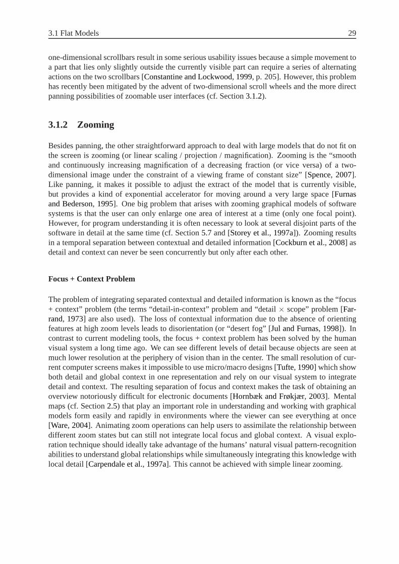
3.1 Flat Models 29
one-dimensional scrollbars result in some serious usability issues because a simple movement toa part that lies only slightly outside the currently visiblepart can require a series of alternatingactions on the two scrollbars [Constantine and Lockwood, 1999, p. 205]. However, this problemhas recently been mitigated by the advent of two-dimensional scroll wheels and the more directpanning possibilities of zoomable user interfaces (cf. Section 3.1.2).
3.1.2 Zooming
Besides panning, the other straightforward approach to deal with large models that do not fit onthe screen is zooming (or linear scaling / projection / magnification). Zooming is the “smoothand continuously increasing magnification of a decreasing fraction (or vice versa) of a two-dimensional image under the constraint of a viewing frame ofconstant size” [Spence, 2007].Like panning, it makes it possible to adjust the extract of the model that is currently visible,but provides a kind of exponential accelerator for moving around a very large space [Furnasand Bederson, 1995]. One big problem that arises with zooming graphical modelsof softwaresystems is that the user can only enlarge one area of interestat a time (only one focal point).However, for program understanding it is often necessary tolook at several disjoint parts of thesoftware in detail at the same time (cf. Section5.7and [Storey et al., 1997a]). Zooming resultsin a temporal separation between contextual and detailed information [Cockburn et al., 2008] asdetail and context can never be seen concurrently but only after each other.
Focus + Context Problem
The problem of integrating separated contextual and detailed information is known as the “focus+ context” problem (the terms “detail-in-context” problemand “detail× scope” problem [Far-rand, 1973] are also used). The loss of contextual information due to the absence of orientingfeatures at high zoom levels leads to disorientation (or “desert fog” [Jul and Furnas, 1998]). Incontrast to current modeling tools, the focus + context problem has been solved by the humanvisual system a long time ago. We can see different levels of detail because objects are seen atmuch lower resolution at the periphery of vision than in the center. The small resolution of cur-rent computer screens makes it impossible to use micro/macro designs [Tufte, 1990] which showboth detail and global context in one representation and rely on our visual system to integratedetail and context. The resulting separation of focus and context makes the task of obtaining anoverview notoriously difficult for electronic documents [Hornbæk and Frøkjær, 2003]. Mentalmaps (cf. Section2.5) that play an important role in understanding and working with graphicalmodels form easily and rapidly in environments where the viewer can see everything at once[Ware, 2004]. Animating zoom operations can help users to assimilate the relationship betweendifferent zoom states but can still not integrate local focus and global context. A visual explo-ration technique should ideally take advantage of the humans’ natural visual pattern-recognitionabilities to understand global relationships while simultaneously integrating this knowledge withlocal detail [Carpendale et al., 1997a]. This cannot be achieved with simple linear zooming.

30 Chapter 3. Complexity of Graphical Models
Zoomable User Interfaces
The rapid zooming technique that is employed by zoomable user interfaces (ZUI) attempts toexploit the user’s mental map and short term memory to provide context by only showing a smallfocus region like an ordinary zoom, but allowing the user to zoom-out very quickly to a low-detail context view and then zoom back in quickly to another focus region.Furnas and Bederson[1995] use the term “highly zoomable interfaces” for this class oftechniques whileWare[2004]calls them “rapid zooming techniques”. The main characteristics of zoomable user interfaces arethat (i) the information objects are organized in space and scale and (ii) users interact directlywith the information space, mainly through panning (which changes the area of the informationspace that is visible) and rapid zooming (which changes the scale at which the information spaceis viewed) [Hornbæk et al., 2002]. The first popular implementation of very fast zooming wasthe ”Pad“ system [Perlin and Fox, 1993] which additionally employs a “semantic zoom” so thatthe user sees different representations of an element when the magnification factor changes. Forexample, an element can appear as a rectangle if there is onlylittle real-estate available and, as itgrows, as a page of text. Elements can also disappear completely if they become too small. Thistechnique of a logical or semantic zoom [Herot, 1980] generates a new representation when thezoom level changes instead of just globally scaling the whole representation.
A multitude of implementations of zoomable user interfaceshave been proposed over time (e.g.,Pad++ [Bederson and Hollan, 1994], Jazz [Bederson et al., 2000], Piccolo [Bederson et al.,2004b], ZVTM [ Pietriga, 2005], MuSE [Furnas and Zhang, 1998]) and the technique has recentlyagain gained a lot of attraction trough popular geographic information systems like Google Earth.An experimental evaluation of ZUI for software visualization ofSummers et al.[2003] indicatesthat subjects perform better (i.e., faster and with fewer errors) by using rapid zooming techniquesat understanding visual programs than with traditional zoom techniques. However, the directinteraction that is an essential part of ZUI’s can become a problem if the model is editable as theuser has to indicate whether he wants to move a node (or a set ofnodes) or just the viewport.
Concurrent Control of Pan and Zoom
While traditional interfaces often combine panning and zooming, the two are usually controlledindependently. This separation often results in a cascade of zoom and pan actions and therebya cumbersome interaction. In order to overcome this problem, the approach ofBourgeois andGuiard[2002] assigns panning and zooming to two independent devices controlled by differenthands to permit parallel control of zoom and pan. The “OrthoZoom Scroller” ofAppert andFekete[2006] is a one hand variant of this approach for one-dimensional (vertical) scrolling.It maps the vertical mouse movements to vertical panning andhorizontal mouse movements tozooming. A different approach to connect zooming and panning is to automatically calculateone of the two from the user’s manipulation of the other. The “depth modulated flying” (DMF)by Ware and Fleet[1997] automatically adapts the viewer’s scroll velocity in response to hiscontrol of altitude (the zoom level).Tan et al.[2001] inverted the speed/zoom coupling with

3.1 Flat Models 31
the “speed-coupled flying with orbiting” in which the altitude (or zoom level) is automaticallyadjusted in response to the scroll velocity. The experimentof Cockburn and Savage[2003] showsthat scrolling tasks are solved significantly faster with such an automatic zooming in both textdocument and map browsing tasks.
3.1.3 Overview + Detail
While zooming separates contextual and detailed information temporally, a small overview (or“map view”) combined with a large detailed window separatesthem spatially. The idea of com-bining a small panoramic overview (the “world view monitor”) and a large detailed screen goesback to the “Spatial Data Management System” [Donelson, 1978] developed in the 70’s at theMIT. The user interacts with the two views separately, although actions in one are usually imme-diately reflected in the other. This tight coupling between the overview and the detail view forbidsan independent exploration of the two views. Recently, the boundary between such overviewsand traditional scrollbars has been blurred by thumbnail document overviews that show smalloverviews of the pages of a document as part of the scrollbar.
A critical factor of this technique is the size of the overview window as it influences how muchinformation can be seen in the overview and how easy it is to navigate in it. However, a largeoverview window might take too much screen real-estate fromthe detail window [Hornbæk et al.,2002]. This problem worsens with the size of the model, because the gap between the abstractionlevel in the overview and the detail view widens [Berner, 2002]. Some approaches allow the userto control the size of the overview to mitigate this trade-off.
A more fundamental problem is the integration of the two views that has to be done solely by theuser. He has to figure out constantly where the small view fits in the big picture (even though thelocation and size of the detail window are usually indicatedin the overview window) and whatvisible features correspond [Furnas, 1981] because an explicit connection between the detailand overview view is missing [Spence, 2007]. An experiment byHornbæk et al.[2002] indeedshowed that an overview slows users down. They suggest several explanations for the results: theoverview might be visually distracting, switching betweenthe detail and the overview windowrequires a mental effort and time to move the mouse or the overview window may have beento coarse (the overview window did not support fine-grained navigation). A second experiment[Hornbæk and Frøkjær, 2003] supported the first one insofar as subjects were slower at answeringquestions about an electronic (text) document with an overview + detail interface than with alinear interface. Interestingly, subjects scored significantly better in some tasks and stronglypreferred the overview + detail interface. These findings were not supported by the experimentof Pietriga et al.[2007] which indicates that pan and zoom combined with an overviewis moreefficient than classical pan + zoom. Their work explicitly aims to eliminate cognitive skills andaddressing motor and perceptual skills only (i.e., the subjects had to look for rectangles withrounded corners in a set of rectangles with square corners).However, exactly these cognitiveaspects may cause interaction effects between the type of the task and the interface in real use.

32 Chapter 3. Complexity of Graphical Models
3.1.4 Distortion
The main problem with both zooming and overview + detail is the separation between contextualand detailed information (temporal in the case of zooming and spatial for overview + detail)which places the demanding task of integrating the two solely on the user’s shoulders. Distortion-oriented techniques aim to avoid this separation by displaying the focus within the context in asingle continuous view. Presenting all regions in a single coherent display is meant to reducethe short term memory load associated with mentally integration distinct views and thereforepotentially improve the user’s ability to comprehend and manipulate the information. Since thescreen (or more precisely its resolution) is usually not bigenough to show the complete model,distortion-oriented techniques show the detailed information in a magnified focus region, whileits surrounding regions present the global context at reduced magnification [Leung and Apperley,1994]. In contrast to the conventional linear zoom (cf. Section3.1.2), these techniques applydifferential scale functions (i.e., nonlinear magnification) across the information surface, leadingto intentional distortion. Thus, distortion-based tools provide space for the magnification oflocal detail by compressing the rest of the image [Carpendale et al., 1997a]. The loss of displayarea that results from the magnification of one or multiple parts of the image is compensatedby the same amount of demagnification in other parts of the image. Otherwise, the area of theimage would grow. A distorted view is generated by applying amathematical function (thetransformation function) to an undistorted image. This transformation function defines how theoriginal image is mapped to the distorted view.
The application of distortion-oriented techniques to computer-based graphical data goes back toFarrand[1973]. However, the concept of distortion or deformation has been used over many cen-turies by cartographers in various map projections (see e.g., [Tufte, 1990, p. 12]). One exampleis Harry Beck’s famous London Underground map. Beck realized that the exact geographic loca-tion and the distance between the stations can be abstractedaway, even though this two seem tobe fundamental properties of a map. Subsequently, he was able to freely distort the map preserv-ing only the correct sequence of the stations which resultedin a much simpler and cleaner map.Leung and Apperley[1994] classify such distortion-oriented presentation techniques accordingto their magnification function in two distinct classes: techniques that have piecewise continu-ous magnification functions and techniques with continuousmagnification functions. Two tech-niques with piecewise continuous magnification functions,the “Bifocal Display” and the “Per-spective Wall”, as well as one with a continuous magnification function, the “Graphical FisheyeViews”, are presented in the following. We cover here only 2Dtechniques, a distortion-orientedtechnique for 3D can be found in [Carpendale et al., 1997a].
Bifocal Display
The Bifocal Display ofSpence and Apperley[1982] represents the information space by employ-ing the analogy of a sheet of paper which is folded to compressbut still show the outer portionswhile leaving the center visible in full detail. The interaction with it can be described by the

3.1 Flat Models 33
metaphor of a paper stretched across four rollers, with two of them in the foreground giving arectangular focal region and the other two rollers on eitherside giving receding side-plate dis-plays. The user can now change the focus by sliding the paper in either direction. The BifocalDisplay is relatively simple to implement and does provide spatial continuity between regions.However, it has the disadvantage of discontinuities of magnification at the boundaries betweenthe detailed and the distorted view [Leung and Apperley, 1994]. Additionally, the information inthe distorted regions of the Bifocal Display is often hard todecipher. That is not really an issuesince the primary purpose of the distorted views is to let theuser notice that there is some moreinformation (i.e., awareness and identification). Text andother details that are unreadable canalso be suppressed in the distorted regions which results ina kind of semantic zoom.
Perspective Wall
The Perspective Wall ofMackinlay et al.[1991] (and its successor the Document Lens [Robert-son and Mackinlay, 1993]) upgrades the Bifocal Display with smooth transitions. Two sidepanels to the left and the right of the central panel show a distorted view of the out-of-focusregions by a direct demagnification that is proportional to their distance from the viewer. In con-trast, the Bifocal Display has a constant demagnification factor. Therefore, the Bifocal Displayis actually a special case of the Perspective Wall [Leung and Apperley, 1994].
Graphical Fisheye Views
The basic idea behind the Graphical Fisheye Views ofSarkar and Brown[1992] goes back tothe Polyfocal Projection ofKadmon and Shlomi[1978] which uses the analogy of a map thatis printed on a rubber sheet which is then pushed from behind at the focal point(s). The termfisheye stems from George W. Furnas’ analogy to a very wide angle or fisheye lens (cf. Section3.3.3andFurnas[1986]). Sarkar and Brown proposed two different implementations, one basedon a Cartesian coordinate system and the other on a polar system for the transformation1. Fig.3.1shows an example of a polar Fisheye View with the focus on theCabinControllercomponent.
Graphical Fisheye Views (or more generally presentation techniques with a continuous magnifi-cation factor) tend to distort the boundaries of the transformed image heavily because the image istransformed radially rather than independently in the x andy directions. This distortion increaseswith a bigger magnification factor [Leung and Apperley, 1994]. Users sometimes perceive theresulting Graphical Fisheye Views as too distorted and unnatural so that spatial comprehensioncan suffer a lot [Carpendale et al., 1997b]. Adding cues (e.g., simple parallel grid lines) hasbeen proposed to enhance the user’s spatial comprehension of the distorted space [Zanella et al.,2002]. A second problem are difficulties in target acquisition because the lens displaces itemsaway from the actual screen position used to activate them. Thus, objects appear to move away
1The transformation was applied only to the nodes of a graph structure in order to avoid that straight lines andrectangles are transformed into curved lines and curvilinear rectangles respectively.

34 Chapter 3. Complexity of Graphical Models
Figure 3.1: Graphical fisheye view of a simple software system model
as the focus approaches them (the so called “moving target” problem [Gutwin, 2002]). And fi-nally, the interaction can become very cumbersome if Graphical Fisheye Views are applied onthe model while it is edited because the interaction is not direct anymore but goes through thefisheye lens [Donskoy and Kaptelinin, 1997].
A number of experimental evaluations have been conducted during the last years in order tocompare Fisheye Views with more traditional interfaces leading to contradictory results. Thefisheye technique was significantly faster than either traditional zooming or panning for multi-point interactions in the experimental validation ofShoemaker and Gutwin[2007]. However, itremains unclear whether the improved performance was caused by the fisheye lens or the multiplefocal points, because the control interface did not allow multiple focal points. Büring et al.[2006] compared a fisheye view and a traditional pan and zoom for searching scatterplot graphson a mobile device, finding no significant difference in task times, but the subjects stronglypreferred the fisheye interface (which actually contradicts [Baudisch et al., 2004; Donskoy andKaptelinin, 1997; Gutwin and Fedak, 2004; Hornbæk and Frøkjær, 2003]). They suggest thatthe positive findings may be due to the nature of the task in theexperiment which did not requirerelative spatial judgments. The task dependent results in the evaluation of fisheye views havealso been shown in the study ofGutwin and Fedak[2004]. They compared a single-focus fisheyeinterface with a two level zoom and a pan interface for three tasks: image editing, web browsingand network monitoring. The fisheye interface best supported navigation, while the zooming
3.2 Horizontal Abstraction 35
interface best supported monitoring and the traditional pan was the slowest interface for all threetasks. The results ofNekrasovski et al.[2006] were that pan and zoom was significantly fasterthan the focus + context technique. An additional overview did not impact task times, but thesubjects favored an overview (which is supported by the findings of Hornbæk et al.[2002]).Furthermore,Donskoy and Kaptelinin[1997] showed that zooming outperforms fisheye viewsfor tasks that involve identification and drag-and-drop manipulation of icons, which indicatesthat fisheye views can become problematic for interfaces requiring interactions which go beyondpure navigation (e.g., editing).
The idea of distorting the contextual information has also been applied to text (e.g., the “FisheyeMenus” ofBederson[2000]). The evaluation of a linear, fisheye and overview + detail interfacefor reading electronic text documents byHornbæk and Frøkjær[2003] showed that the fisheyeview encouraged faster reading, but at the expense of lower comprehension. The overview in-terface allowed the users to navigate the document rapidly,and although they spent more timereading, they scored better in comprehension tests (these results were supported byBaudischet al. [2004]). Additionally, the linear interface for reading electronic text documents was infe-rior on most usability aspects compared to an overview+detail and fisheye interface. However,a following experiment with fisheye menus [Hornbæk and Hertzum, 2007] revealed that usersmake little or no use of the non-focal display region of fisheye menus and that performance withfisheye menus is inferior to traditional hierarchical menuswhich also points to the power andimportance of a hierarchical structure (cf. Section3.3).
3.2 Horizontal Abstraction
The techniques described so far address primarily the spatial problem (i.e., space limitation) thatarises with large and complex graphical models. Dealing with the information density problemrequires to take additional semantic information about themodel into account in order to supportadditional abstractions. One such abstraction that is usedfrequently for graphical models ofsoftware systems is to provide views on the system from different perspectives [Kruchten, 1995].These orthogonal views [Kim et al., 2000] on the description of a complete system are usuallyshown in separate diagrams. Typical views are a static or structural view that shows the structureof the system and a dynamic or a behavior view that describes how the system or its componentsperform over time. We use the term horizontal (or partitioning) abstraction [Berner, 2002] for thisaspectual decomposition because the abstraction takes place within one hierarchical level. Thecomplementary vertical abstraction of information on different hierarchical levels is discussed inSection3.3.
The multi-diagram approach has been established as the de facto standard way to deal withthe spatial and information density problem during the modeling of software systems by theUML (cf. Section2.2.2). The smaller subdiagrams reduce the cognitive and perceptual overload,but introduce the problem of cognitive integration [Dori, 2002; Kim et al., 2000; Storey et al.,1997a]. The horizontal decomposition improves the understandability of individual aspects of

36 Chapter 3. Complexity of Graphical Models
the system, but it may reduce the understanding of the systemas a whole. As a consequence, thenotation must provide explicit mechanisms for conceptual integration [Kim et al., 2000] to allowthe reader the combine information from different diagramsinto one coherent mental represen-tation of the problem or system. This integration problem (or model multiplicity problem [Pelegand Dori, 2000]) comprises two subproblems [Kim et al., 2000]: First, during theperceptualintegrationthe user has to establish the interdependence between the relevant system elementsthat have been dispersed across multiple diagrams. And second, theconceptual integrationcov-ers the generation and refinement of hypotheses about the system by combining the informationinferred from the diagrams. The integration problem worsens with the fact that users often workon a small subset of the whole model, but on all aspects of thissubset simultaneously. Theperceptual and conceptual integration process can be supported by incorporating visual cues andcontextual information in the diagrams as representation aids. One example of such aids are linesthat connect the representations of the same element in different diagrams [Huotari et al., 2004].
A second, related problem are the frequent “context switches” [Donoho et al., 1988] that occurbecause the user is forced to constantly flip back and forth between two or more related dia-grams.Henderson and Card[1986] use the term “thrashing” for this problem. Spatial contiguitycan solve this problem by showing related diagrams simultaneously in the visual field [Moody,2006]. This replaces a costly cognitive process (maintaining the information about the relationsin working memory) with a much faster perceptual process (visual scanning). However, it isusually not possible to achieve such a visual contiguity on (small) computer screens. An ad-ditional more technical problem is maintaining the inter-diagram consistency to make sure thatinformation concerning the same elements are consistent indifferent diagrams since the viewsemployed by the different diagrams are usually not independent [Kruchten, 1995]. And finally,the main problem with a horizontal abstraction is that the individual diagrams can still grow verylarge without a sound hierarchical decomposition mechanism. Such hierarchical decompositionsare the topic of the next section.
3.3 Vertical Abstraction
Probably the most successful way to deal with large and complex systems is a hierarchical de-composition. It breaks a complex system down into parts thatare easier to conceive, understandand maintain. This divide and conquer approach is used in a wide variety of disciplines todeal with complexity (e.g., modularization in the system design and programming field [Parnas,1972], segmentation in cartography or research in natural sciences in general [Simon, 1996]). Ahierarchical decomposition that follows the principle of minimizing the coupling between partswhile maximizing the cohesion of the individual parts allows to look at a system at differentlevels of detail while treating some parts as blackboxes (i.e., abstracting from their internals).We use the term vertical abstraction [Berner, 2002] for this form of abstraction that is based ondifferent hierarchical levels. A hierarchical decomposition of a system’s model into parts of man-ageable and understandable size has been one of the central pillars in the modeling of software

3.3 Vertical Abstraction 37
systems for years (cf. Section2.2.1). But it had to take a back seat during the last years due tothe lack of a clear decomposition construct in the UML. Only recently, with the large overhaul inversion 2.0, has the OMG reclaimed the importance and power of hierarchical decompositions[Kobryn, 2004].
3.3.1 Graphical Representations of Hierarchical Decompositions
If only the hierarchical (i.e., parent-child) relationships are considered, a representation of ahierarchical decomposition as graph structure yields a tree (cf. Section2.1.3). Thus, standardgraphical notations for drawing trees such as graph trees ornested sets [Knuth, 1997, page 308]can be used to show hierarchical decompositions graphically.
Graph Tree
In a graph tree, all relationships, including hierarchicalones, are represented as edges and repre-sented graphically as lines. The classical tree layout convention (see e.g. [Herman et al., 2000]for a survey of tree visualizations) which is for example employed in organization charts drawssuch a tree in a level fashion with the top level (i.e., root ofthe node) at the top. A decompositioncan be represented graphically as tree by showing the part (component) as child of the whole(composite) node. The main drawback of the classical tree layout is that it becomes clutteredand unusable for large trees.Robertson et al.[1991] proposed “Cone Trees” as a solution tothis problem by presenting the hierarchy in 3D to better exploit the available space. A hierarchyis laid out uniformly in three dimensions with a node at the top and its children placed evenlyalong the base of a cone. The additional dimension reduces the aspect ratio compared with atree laid out in 2D. However, the interaction becomes more complex than in a 2D layout of thesame tree. Another approach, the “Hyperbolic Tree Browser”of Lamping et al.[1995] useshyperbolic geometry to visualize large trees. The hyperbolic tree browser stimulated the inter-est in using focus + context techniques for search tasks whena team using it outperformed fiveteams using competing browsers in a “browse-off” panel session at ACM CHI’97 [Mullet et al.,1997]. However, previous studies had failed to show significant advantages of the hyperbolic treebrowser [Czerwinski and Larson, 1997; Lamping et al., 1995]. The studies ofPirolli et al. [2001,2003] uncovered interaction effects between task and interfacefactors, with the hyperbolic treeperforming well on tasks with strong scent, but performing poorly when scent is weak. Anotherway to deal with a large number of nodes in a graph tree is to directly employ vertical abstractionby expanding and collapsing branches of a tree dynamically [Plaisant et al., 2002].
Nested Sets
As an alternative to the classical tree layout, the nested set notation (or “inclusion tree layoutconvention” [Battista et al., 1994]) follows the concept of Venn or Euler diagrams by visually

38 Chapter 3. Complexity of Graphical Models
representing the parent-child relationship by the child node being completely contained withinthe parent node. The notation is supported by the theory of pattern perception: The Gestalt prin-ciple of closure states that a closed contour tends to be seenas an object and that there is a verystrong perceptual tendency to divide regions of space into “inside” and “outside” [Ware, 2004].A region that is enclosed by a contour becomes a common regionwhich is a much stronger or-ganizing principle than for example proximity. Additionally, the semantics of the hierarchicaldecomposition become obvious as all children are removed automatically if the parent is re-moved. In contrast, the notation for composition and aggregation in UML class diagrams usesconnecting lines instead of nested symbols. Additionally,the whole and its parts are shown onthe same level. Thus, the Gestalt law of closure cannot be exploited which results in lengthy ex-planations and discussion of UML’s aggregation and composition concepts. UML’s compositionand aggregation notation uses arbitrary symbols (cf. Section 2.2). In contrast to these arbitrarysymbols, sensory symbols like graphically nested symbols derive their expressive power fromtheir ability to use the perceptual processing power of the brain without learning [Ware, 2004].The empirical evaluation of different representations of aggregation (or composition) byIraniet al. [2001] has revealed that the semantics that are inherent in the different kinds of relation-ships of real-world objects should also be applied to the abstract concepts in diagrams. Anotheradvantage of the nested set notation is that some of the relationships (i.e., the parent-child rela-tionship) between nodes are represented implicitly by the nested structure and do not have to beshown explicitly by a link which improves the readability ofthe diagram (by reducing the num-ber of symbols). Furthermore, nodes can be summarized (i.e., vertically abstracted) by drawingthe node rectangle without its contents.
One drawback of the nested set notation is that only one kind of hierarchical relationship can berepresented by the nested symbols. If there are additional kinds of hierarchical relationship, theyhave to be depicted as lines between the nodes. Some approaches propose to show multiple kindsof hierarchical relationships directly by the nested set notation: The Higraph notation [Harel,1988] represents both generalization and aggregation with nested boxes by dividing a node bydotted lines. And the Hicon approach [Sindre et al., 1993] shows several orthogonal hierarchicalrelations at the same time by a symbolic distinction of nodes(e.g., squares for aggregation andcircles for generalization).
An additional problem is that the recognition of the hierarchical structure can become problem-atic with the nested set notation if only parts of the nodes are visible or connecting lines areconfused with node boundaries. A possible solution is a simple shading of the nodes which al-ternates with the levels of the hierarchy (see Figure3.4 on page44). This exploits the Gestaltlaws of figure-ground effects [Ware, 2004] that contribute to the perception of a figure becausea node is now the figure on one and the ground on the next lower level. The shading of thehierarchy shifts some of the user’s cognitive load to his perceptual system (i.e., substitutes see-ing for reasoning). The way in which the visual system divides the world into regions is calledsegmentation [Ware, 2004]. According to the Gestalt laws of perception, the capacityof theworking memory is limited by the number of chunks and not the size of each individual chunk[Moody, 2006]. Therefore, organizing the diagram elements in perceptual groups increases the

3.3 Vertical Abstraction 39
number of elements that can be shown in the diagram without overloading the working memory.Conversely, a missing structure or grouping of diagram elements requires each diagram elementto be encoded as a separate chunk in working memory.
3.3.2 Explosive Zoom
Most current modeling tools allow the user to interact with hierarchically structured models rep-resented in the nested set notation by what we call “explosive zooming” (or “multiple views”[Storey et al., 1997a]): when looking at the details of a particular node, the diagram with thedetails either replaces the previously displayed diagram or it is opened in a new window thatsupersedes the previously viewed one [Berner, 2002]. Thus, every level of the hierarchy consistsof a set of separate diagrams which results in a cascading hierarchy of diagrams [Huotari et al.,2004]. In contrast to the traditional linear scale or zoom (cf. Section 3.1.2), the explosive zoomemploys a structural zooming by exploiting the hierarchical structure of the presented informa-tion. The basic idea is to divide a single, large diagram along its decomposition structure intoa set of smaller subdiagrams of manageable size. It is often recommended that this manageablesize should be based on the limits of human information processing where the major constraint isthe capacity of the working memory, which is believed to be “seven plus or minus two” [Miller ,1956].
Explosive zooming has the big drawback that the context of the zoomed node is lost: one cannotview the details of a node and its context in the same diagram.For human understanding of dia-grams, this is bad because humans typically want to see theirfocus of interest in detail togetherwith its surrounding context. The resulting integration problems are similar to those of tradi-tional zooming (cf. Section3.1.2), overview + detail interfaces (cf. Section3.1.3) as well as thehorizontal abstraction technique (cf. Section3.2). Explosive zooming worsens these problems asit results in temporaland spatial separation. This is similar to hypertext systems with the sameproblem of not knowing one’s location in the space and getting lost: clicking a hypertext linkgenerates an entirely new screenful of information. The cognitive cost of such a simple interac-tion is that the entire information context has changed, andthe new information may be presentedusing a different visual symbol set and different layout conventions. As a result, several secondsof cognitive reorientation may be required afterwards [Ware, 2004].
Diagrams are especially well suited to understand information (especially structural relation-ships) in parallel. The explosive zoom undoes this advantage as relationships over diagramboundaries are not visible. One possibility to mitigate this problem is the use of redundancy toachieve vertical integration, by employing foreign elements with a link back to their home dia-grams whenever an element has a connection to an element in another diagram [Moody, 2006].However, showing the same model element in different diagrams results in additional integrationand consistency management problems. The emphasis of the UML on a horizontal abstractiontogether with its adoption of hierarchical decompositionsin version 2.0 (the arbitrarily deeplynested hierarchical structures in composite structure diagrams, activity diagrams and state ma-

40 Chapter 3. Complexity of Graphical Models
chine diagrams) has prompted many tool vendors to combine explosive zooming with the alreadyemployed scattering of different system aspects over multiple diagrams. This forces the user tomentally integrate horizontally (diagrams at the same level of the hierarchy) as well as vertically(diagrams at different levels of the hierarchy).
3.3.3 Suppression
While the horizontal and vertical abstraction as discussedso far use only the structure of themodel to decide which elements are shown in the current view,the “suppression” [Spence, 2007]or “elision” [Ware, 2004] techniques take additionally the position of the beholderinto account.The basic idea has been illustrated tellingly by Saul Steinberg in his famous New Yorker maga-zine cover “View of the World from the 9th Avenue”, giving a Manhattanite’s selective view ofthe world:
Figure 3.2: Saul Steinberg’s “View of the World from the 9th Avenue”
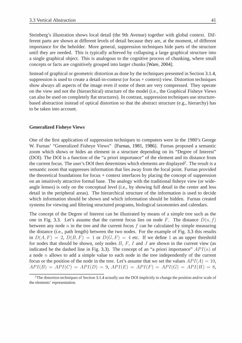
3.3 Vertical Abstraction 41
Steinberg’s illustration shows local detail (the 9th Avenue) together with global context. Dif-ferent parts are shown at different levels of detail becausethey are, at the moment, of differentimportance for the beholder. More general, suppression techniques hide parts of the structureuntil they are needed. This is typically achieved by collapsing a large graphical structure intoa single graphical object. This is analogous to the cognitive process of chunking, where smallconcepts or facts are cognitively grouped into larger chunks [Ware, 2004].
Instead of graphical or geometric distortion as done by the techniques presented in Section3.1.4,suppression is used to create a detail-in-context (or focus+ context) view. Distortion techniquesshow always all aspects of the image even if some of them are very compressed. They operateon the view and not the (hierarchical) structure of the model(i.e., the Graphical Fisheye Viewscan also be used on completely flat structures). In contrast,suppression techniques use structure-based abstraction instead of optical distortion so that theabstract structure (e.g., hierarchy) hasto be taken into account.
Generalized Fisheye Views
One of the first application of suppression techniques to computers were in the 1980’s GeorgeW. Furnas’ “Generalized Fisheye Views” [Furnas, 1981, 1986]. Furnas proposed a semanticzoom which shows or hides an element in a structure dependingon its “Degree of Interest”(DOI). The DOI is a function of the “a priori importance” of the element and its distance fromthe current focus. The user’s DOI then determines which elements are displayed2. The result is asemantic zoom that suppresses information that lies away from the focal point. Furnas providedthe theoretical foundations for focus + context interfacesby placing the concept of suppressionon an intuitively attractive formal base. The analogy with the traditional fisheye view (or wide-angle lenses) is only on the conceptual level (i.e., by showing full detail in the center and lessdetail in the peripheral areas). The hierarchical structure of the information is used to decidewhich information should be shown and which information should be hidden. Furnas createdsystems for viewing and filtering structured programs, biological taxonomies and calendars.
The concept of the Degree of Interest can be illustrated by means of a simple tree such as theone in Fig.3.3. Let’s assume that the current focus lies on nodeF . The distanceD(n, f)between any noden in the tree and the current focusf can be calculated by simple measuringthe distance (i.e., path length) between the two nodes. For the example of Fig.3.3 this resultsin D(A, F ) = 2, D(B,F ) = 1 or D(G,F ) = 4 etc. If we define1 as an upper thresholdfor nodes that should be shown, only nodesB, F , I andJ are shown in the current view (asindicated be the dashed line in Fig.3.3). The concept of an “a priori importance”API(n) ofa noden allows to add a simple value to each node in the tree independently of the currentfocus or the position of the node in the tree. Let’s assume that we set the valuesAPI(A) = 10,API(B) = API(C) = API(D) = 9, API(E) = API(F ) = API(G) = API(H) = 8,
2The distortion techniques of Section3.1.4actually use the DOI implicitly to change the position and/or scale ofthe elements’ representation.

42 Chapter 3. Complexity of Graphical Models
API(I) = API(J) = 7 andAPI(K) = API(L) = 6 in the tree of Fig.3.3to indicate that thenodes at the top are more important than nodes at the bottom. The Degree of InterestDOI(n, f)which is used to decide whether noden is visible if the focus is on nodef is now calculatedaccording to
DOI(n, f) = API(n)−D(n, f) (3.1)
wheren is the current node,f the current focus,API(n) the a priori interest in noden andD(n, f) the spatial or semantic distance between nodesn and f . For Fig. 3.3 this results inDOI(A, F ) = 8, DOI(K,F ) = 4 or DOI(D,F ) = 6 and only the nodes within the dottedline are shown in the current fisheye view if we set the lower threshold to5. The DOI functionis an information suppression function and Furnas’ approach therefore explicitly attacks the in-formation density problem of graphical models. Thus, Generalized Fisheye Views create a kindof “information distortion” [Leung and Apperley, 1994] instead of a graphical or geometricaldistortion. Probably the biggest drawback of Furnas’ approach is that it supports only one focusat a time which is often not enough for the understanding of software structures. A hierarchicalstructure is not strictly necessary for the Generalized Fisheye Views, but Furnas’ original publi-cation introduces “the tree fisheye DOI” and the technique abstracts vertically (which is also thereason why it is introduced in this section).
A
B C D
FE
JI
LK
HG
Figure 3.3: Generalized Fisheye View of a simple tree
Manual controls for collapsing and expanding program statement blocks and methods are nowstandard in most Integrated Development Environments (IDE). But automatic expansion andcontraction using a DOI algorithm is still a research topic,as for example the Mylar tool [Kerstenand Murphy, 2005]. Jakobsen and Hornbæk[2006] developed a fisheye source code viewer

3.3 Vertical Abstraction 43
that uses a DOI function to automatically display/suppresscode blocks depending on the user’scurrent focus. They found in an experimental comparison between the fisheye interface and astandard linear list view that the fisheye view not only resulted in significantly less time neededto fulfill a task but was also preferred to the linear listing.The concept has also been appliedto other structures such as the “Table Lens” ofRao and Card[1994] which presents a compactoverview of large tabular data, displaying all rows an columns simultaneously by showing valuesas small bars. Rows and columns can be selectively expanded to show the actual data values.Such expansions can be applied independently to rows and columns, allowing multiple focalpoints, while preserving the rectangular shape of cells.Bederson et al.[2004a] later applied theTableLens concept to a calendar in their “DateLens” approach .
3.3.4 Combined Distortion and Suppression
Furnas’ DOI determineswhat information should be shown (the original formulation has noexplicit control over the attributes that define the graphical layout), while much of the subsequentresearch addressed the issue ofhow the information is presented [Furnas, 2006]. The basicapproach has been to apply an information suppression technique concurrently with a distortion-oriented technique to solve the spatial and information density problem at once [Carpendale et al.,1997a; Leung and Apperley, 1994]. Furnas’ fisheye views can be applied to graphical modelswhile avoiding the distortions that occur with nonlinear magnifications (cf. Section3.1.4) bychanging only the scale and/or position of an element but never its overall shape (i.e., a rectangleis still a rectangle after the distortion). If the model usesthe nested set notation, fisheye viewscan be generated by collapsing subtrees of related nodes andedges into a single node to showdifferent parts of the model at different levels of detail. Fig. 3.4 shows an example of such afisheye view on a nested hierarchical graphical model.
The heart of such a fisheye view technique is its zoom algorithm which adapts the layout ifa currently visible node is suppressed or a hidden node shown. By zooming-inandzooming-out, the user can control the level of detail of each node. Fig.3.4a) shows an abstract viewof a hierarchical model: only the three top-level nodesA, B andC are visible. The ellipsisafter a node name indicate that the node has an inner structure which is hidden in the currentview. By successively zooming-in nodesB andD, we get a view, shown in Fig.3.4b), whichshows the details of the model in a focal point (nodeD) together with the global structure of themodel. Conversely, by zooming-out nodes in an expanded model we get a more abstract view.This concept of zooming-in and -out is not new, it has for example already been proposed byHarel for his statecharts [Harel, 1987]. Robertson et al.[1991] call them “gardening operations”because they prune and grow the view of a tree. The terms that are used to describe the resultingviews vary widely among different authors, besides the already used “fisheye view” and “focus+ context view” these are “detail-in-context view” [Carpendale et al., 1997a], “multiscale view”(i.e., different sections of the information are displayedat different scales) [Furnas and Bederson,1995] or “distortion view” [Leung and Apperley, 1994].

44 Chapter 3. Complexity of Graphical Models
A...
G
H
D
E...
F...
B
C...
A...
B...
C...
(a)
(b)
Figure 3.4: Fisheye zooming
45
CHAPTER 4
ADORA
Most current modeling tools rely on flat or practically flat models (i.e., they show all elementsin one view) and support only panning and scaling for navigation (cf. Section3.1). Tools thatsupport a navigation trough the hierarchical decomposition of a model visualize only one levelof the hierarchy using an explosive zoom (cf. Section3.3.2). Given this state of tools, it is notsurprisingly that most modeling languages rely on the principle of loosely couple multi-diagrammodels as the primary means for separating concerns and decomposing large models into man-ageable parts. Since tools do not really support hierarchical and aspectual decompositions oflarge models, decomposition techniques can be provided on the language level only. The basicidea of the ADORA1 approach is to reverse these principles by using an integrated, inherently hi-erarchical model instead of a loose collection of diagrams and a tool that generates abstractionsand diagrams of manageable size. This chapter gives a short overview over the language (Section4.1) and tool concepts (Section4.2).
4.1 The ADORA Language
ADORA has been developed at the Requirements Engineering Research Group of the Univer-sity of Zurich as a language for modeling requirements and, in later stages of the developmentprocess, architectural design specifications on the logical level [Berner, 2002; Glinz et al., 2002;Joos, 1999; Meier, 2009; Seybold, 2006; Xia, 2005]. The driving force behind its developmentis to think beyond currently established modeling paradigms and languages and to mitigate some
1ADORA is an acronym forAnalysis andDescriptionOf Requirements andArchitectures.

46 Chapter 4. ADORA
of the current modeling problems and anomalies. The following sections give a short overviewover the most important language concepts of ADORA and compares them with the current stateof the art (which is basically UML). A more detailed description of the current state of ADORA
can be found in [Meier, 2009].
4.1.1 Abstract Objects Instead of Classes
Instead of types or classes which are the basis for most object-oriented modeling languages,ADORA is based on abstract objects. Abstract objects are prototypical instances of types orclasses. They stand for the concrete instances and their location in the object structure of asystem. However, since they do not represent objects at runtime, there are no concrete valuesstored in their attributes. Object models are more powerfulthan class models in expressingcomposition relationships [Joos, 1999]: With class models it is not possible to model the contextin which an instance of a class is used. Furthermore, class models fail if more than one object ofthe same class has to be modeled [Glinz, 2000] and are hard to decompose [Glinz et al., 2002].
Another problem with class models are the relationships they support. Riel [1996, p. 53] dis-tinguishes between the following categories of relationships that occur in the object-orientedparadigm: (i) uses relationships, (ii) containment relationships, (iii) inheritance relationships and(iv) association relationships. Out of these only the inheritance relationship is class-based whilethe other three are object-based. The concept of class- and object-based relationships denoteswhether or not all objects of a class have to obey the relationship. Because UML (cf. Section2.2.2) puts the emphasis on inheritance2, the class model is its main cornerstone even thoughthe other types of relationships do not really fit into it (because they represent relations betweenobjects and not classes). UML 2.0 has shifted the focus a little bit from classes to components.However, this has let to a lot of syntactic and semantic overlap between the concept of a classand a component [Kobryn, 2004].
4.1.2 Hierarchical Decomposition
As discussed in Section3.3, a hierarchical decomposition is probably the best way to handle bigmodels and deal with their complexity. In ADORA, abstract objects are recursively decomposedinto objects. Thus, the object concept goes over all levels of the hierarchy and the only thingthat changes is the degree of abstractness: objects on lowerlevels model small parts in detail,while objects on higher levels represent larger parts or thewhole system on an abstract level.This makes is possible to use the same graphical notation in summary and detail diagrams. Otherapproaches in which the concepts differ among hierarchicallevels have to use different notations[Moody, 2006]. Using a fisheye zoom concept on this uniform structure of nested objects results
2UML’s strong emphasis on inheritance has also led to conceptual critic. For example, the fact that inheritancebreaks encapsulation has madeGamma et al.[1995, p. 18f] to recommend favoring object composition over classinheritance.

4.1 The ADORA Language 47
in a full vertical model abstraction mechanism. The user candecide on the level of detail in anypart of the model without any restrictions on the number of levels. While previous versions ofUML relied almost only on horizontal model abstractions, classes and components can finally bedecomposed in UML 2.0 [Kobryn, 2004]. This hierarchical decomposition of structure and be-havior includes black- and white-box views on classes and components which makes is possibleto apply such a zoom approach to UML as well.
4.1.3 Integrated Model
Instead of a hierarchical decomposition, most existing object-oriented modeling languages, withUML as the most prominent example, use a set of more or less loosely coupled diagrams of dif-ferent types to cope with the complexity of the modeled system. While this approach facilitatesa clear separation of concerns, a collection of different models hinders integration and abstrac-tion tasks. The lack of integration on the language level results in more redundancy within thelanguage [Joos, 1999]. Enforcing the horizontal consistency between differentmodels demandsadditional constraints. Furthermore, the whole integration task is simply left to the user who hasto integrate the separate models mentally (cf. Section3.2).
In order to mitigate this problems, ADORA integrates all modeling aspects (structure, data, be-havior, user interaction, etc.) in one single coherent model. This facilitates a strong notation ofconsistency and provides the basis for the development of powerful consistency checking mech-anisms. Additionally, it releases the user, at least partially, from the demanding integration task.UML supports since its significant revision in version 2.0 the cross integration of structure andbehavior. However, other aspects such as the user interaction (expressed with use cases in UML)are still not well integrated with the rest of the language [Kobryn, 2004].
4.1.4 View Concept
While the use of an integrated model facilitates better model understandability, the user is drawnin a flood of information if every element of the model is shownall the time. As most of theseelements are not in the reader’s (current) focus of interest, the cognitive overload can be reducedby showing only the model elements which are of interest at the moment. ADORA supports thisby two visual abstraction mechanisms: (i) the model is decomposed hierarchically (as explainedSection4.1.2), thus allowing the user to select the vertical abstractionlevel. And (ii) ADORA em-ploys a view concept that is based on different aspects (structure, data, behavior, user interaction,etc.) of the system. Thus the complete model is basically an abstract one that is virtually nevershown in a diagram. The concrete diagrams illustrate certain aspects of certain parts of the modelin their hierarchical context. This horizontal model abstraction mechanism is achieved by usingthe basic fisheye zoom algorithm to dynamically generate views by toggling the visibility of oneor more model elements (cf. Section8). Such a view is in the mathematical sense a projection ofthe model. ADORA supports six different views:
48 Chapter 4. ADORA
• The base viewshows the static structure of the system. Its hierarchy of abstract objectsforms the basic structure of an ADORA model. Objects are represented by rectanglesusing the nested box notation (cf. Section3.3.1). This allows the user to represent themodel at any level of abstraction and thus to fully exploit the power of the hierarchicaldecomposition. As the base view represents the basic structure of an ADORA model, it isshown all the time albeit at different levels of detail.
• Thestructural view augments the base view with information about relationships betweenobjects. The ADORA language offers associations to model structural relationships or acommunication channel between two objects. Because associations must reflect the hierar-chical structure of the model, ADORA uses the concept of abstract associations (cf. Section11.1) which represent one or multiple associations on a lower level of abstraction as soonas one of the participating nodes is not visible anymore.
• The abstract behavior of objects is represented by the meansof statecharts [Harel, 1987]in thebehavior view. States are embedded in the base view and represented by roundedrectangles which can be nested. State transitions are shownas arrows connecting the states.
• Theuser view is used to model the system from the viewpoint of the user(s).The interac-tion between the system and objects in its environment is modeled by scenariocharts [Xia,2005]. Scenarios are the ADORA equivalent to UML’s use cases. They are visualized asellipses and can be decomposed into sub-scenarios forming aJackson-like [Jackson, 1975]scenario tree. These scenariocharts are integrated into the base view so that a scenario isplaced inside the node that represents the object the environment object interacts with inthis (sub)scenario.
• The actors in the context of the system are modeled in thecontext view. Actors are repre-sented graphically as hexagons and interact through scenarios with the system. Dependingon the level of abstraction the system is currently shown with, the context view yields acontext diagram showing the system as black box together with its external actors.
• ADORA’s functional view is used to define additional properties (e.g., attributes orop-erations) of objects. The functional view is not shown together with the other views butdisplayed separately because it consists mainly of text.
The view concept of ADORA is similar to the floor plan that is the base view for the civil engi-neering field which is augmented with additional layers (with their own notation) for electricity,heating and other aspects of a building.
4.1.5 Variable Degree of Formality for a Controlled Evolution
ADORA allows its users to adapt the degree of formality in the modelto the difficulty and riskof the problem at hand. All language elements support a variable degree of formality so that

4.2 The ADORA Tool 49
they can be represented informally, semi-formally (which is a mixture of formal and informalelements) or formally. For example, the specification of thebehavior of an object can range frominformal natural language to fully-fledged statecharts. Most of the time a model consists of bothformal and informal constructs while it evolves towards a complete and formal specification.
Such an evolutionary requirements process is explicitly supported by ADORA through a semi-formal simulation of a model [Seybold, 2006]. Any requirements modeling language shouldsupport model evolution because requirements are not complete and clear from the beginningbut have to be elicited and refined over time. Model elements can be marked as intentionallyincomplete in ADORA so that they can be distinguished from elements that are incomplete bymistake (i.e., unintentionally). These incomplete modelscan then be simulated in order to un-cover errors end fill the gaps.
4.2 The ADORA Tool
The ADORA tool does not only facilitate the creation of an ADORA model but is, with its navi-gation capabilities, an integral part of the approach. Thusan implementation of the concepts ina tool is not only desirable but essential. Furthermore, an implementation of the concepts pre-sented in this thesis is necessary to verify their feasibility, identify and correct weaknesses and tovalidate them. The fisheye zoom and line routing concepts have in fact not been developed in apurely theoretical manner but evolved from an iterative mixture of conceptual development andimplementation.
The current version of the ADORA tool prototype is based on the Eclipse3 platform, while itspredecessor was a pure Java implementation. One of the most powerful features of the Eclipseplatform is its plug-in architecture which facilitates theextension of the platform in a clear way.One such extension is the Graphical Editing Framework (GEF)4 which provides a Model-View-Controller framework for the implementation of graphical model editors. The Graphical EditingFramework employs basic support for recurring features of graphical editors (e.g., basic undo orcopy & paste support) which reduces the implementation and especially maintenance load whileit improves the usability of the tool significantly.
A detailed discussion of the ADORA tool can be found in Chapter15 which shows how theconcepts presented in the following chapters have been implemented in the tool.
3http://www.eclipse.org4http://www.eclipse.org/gef


Part II
Fisheye Zooming

53
CHAPTER 5
Desired Properties of a Zoom Algorithm
A zoom algorithm has the responsibility to adjust the layoutof a diagram (i.e., the positionand size of the nodes) if one or multiple nodes are suppressedto reduce the overall complexityof the model or shown to see the details within one part of the model. A set of criteria (ordesired properties) is needed to assess how well different techniques are suited for this task. Thischapter lists the properties that a zoom algorithm should have if it is used for visualizing andediting hierarchical models. The properties are derived from the literature on focus + contextvisualization (cf. Chapter6) and our own previous experience with the ADORA tool (cf. Chapter4.2). The presented properties differ from the aesthetic criteria that are used by the automaticgraph drawing algorithms (cf. Sections2.3.1and2.4) because they are used for layout adjustmentoperations and not the creation of an initial layout.
5.1 Compact Layout
Reducing the complexity and size of diagrams is the main motivation for the work presentedin this thesis. The complexity is reduced by suppressing model elements from the diagram. Incase of the fisheye zoom the internals of a node are hidden oncethe node has been zoomed-out.The white space that becomes available at the position of hidden nodes must be removed by thezoom algorithm to reduce the size of the whole diagram. The sibling nodes of the currently sup-pressed nodes are moved which results in a global distortionof the diagram. This has to be donerecursively if a hierarchical model is represented as a set of nested boxes. The zoom algorithmmust only distort the position of the nodes and not their shape because of the problems with

54 Chapter 5. Desired Properties of a Zoom Algorithm
the readability of text and the recognition of links in classical distortion techniques (cf. Section3.1.4). Producing a compact layout is the rationale for developing a zoom algorithm that reducesthe size of the diagram if a node is zoomed-out [Misue et al., 1995]. However, the demand for acompact layout can also become problematic if some elementsare suddenly too close together oreven overlap with other elements such as links or labels (cf.Chapters11 and14). This trade-offbetween a compact layout on one side and an easily readable and understandable diagram on theother may result in the need for different compacting techniques for different tasks.
Fig. 5.1 illustrates the basic idea of a compact layout: NodesG andH are suppressed fromFig. 5.1a) to get a more abstract view of nodeD in Fig. 5.1b). NodeD shrinks because noneof its children is shown anymore. NodesE andF are moved closer together so that the newlyavailable white space is not wasted. This reduces the space that is required by nodeA to showits children which lets nodeA shrink. The smaller size ofA results in more white space whichcan be used byA’s siblingsB andC. The whole diagram then becomes smaller because nodesB andC are moved closer to nodeA.
G H
DE
F
A
BC
D...
E
F
A
BC
(a)
(b)
Figure 5.1: Produce a compact layout
5.2 Disjoint Nodes
The zoom algorithm is restricted by a set of constraints while it moves nodes to produce a morecompact layout. The most important constraint is that nodeson the same level of the hierarchymust not overlap [Bartram et al., 1995; Misue et al., 1995]. Overlapping nodes reduce the read-ability of the diagram because some informations may be hidden behind nodes. Additionally,it becomes difficult to see the hierarchical relationships between nodes because these relationsare represented as nested boxes. A node that is located inside another node just because the twonodes overlaps compromises this notation.

5.3 Preserve the Mental Map 55
The property of disjoint nodes must hold after any zoom operation regardless of whether a nodeis zoomed-in or out. For the example of Fig.5.1this means that nodesD, E andF (which are onthe second level of the hierarchy) as well as nodesA, B andC (which are on the first level) mustnot overlap in Fig.5.1b) if nodeD is zoomed-out. The same must hold for the inverse operation(i.e., the resulting layout of Fig.5.1a) if nodeD in Fig. 5.1b) is zoomed-in). If the property of acompact layout is the rationale for a zoom algorithm in the case of zoom-out operations, then theproperty of having disjoint nodes is the rationale for zoom-in operations: Zooming-in expandsnodes so that sibling nodes have to be moved away to avoid overlaps. There are essentiallytwo different ways to deal with the property of disjoint nodes: Either the zoom algorithm itselfguarantees an overlapping free layout or overlaps are detected and resolved explicitly after thenodes have been moved by the zoom algorithm.
5.3 Preserve the Mental Map
To maintain the understandability of a model, it is vital that the new layout resembles the originallayout as far as possible after an adjustment of the layout (such as a zoom operation) [Bartramet al., 1995; Carpendale et al., 1997a; Leung and Apperley, 1994; Misue et al., 1995; Noik, 1994;Sindre et al., 1993; Storey and Müller, 1995]. This is important because the modeler builds amental map which consists of the positioning, the size and other user-defined visual propertiesof the model (cf. Section2.5). A new layout that differs too much from the current layout resultsin a spatial disorientation of the user. The layout characteristics that can be used as metrics toformalize the mental map and that should be maintained in an adjusted layout to preserve theuser’s mental map depend on the type of the layout and the application. Thus, they vary widelyamong different authors:
• The relative direction between nodes [Sindre et al., 1993] or the relative location of nodes[Bartram et al., 1995] should be maintained.Eades et al.[1991] andMisue et al.[1995]use the termorthogonal ordering of nodes for this characteristic and try to formalize itby stating that it is preserved if the horizontal and vertical ordering of points is preserved.The position of the center of the nodev is given by its coordinates(xv, yv). The adjustedcoordinates(x′
v, y′
v) and(x′
u, y′
u) of two nodesv andu have the same orthogonal orderingas the coordinates in the original layout if
– xu < xv if and only if x′
u < x′
v and
– yu < yv if and only if y′u < y′v and
– xu = xv if and only if x′
u = x′
v and
– yu = yv if and only if y′u = y′v.
Two layouts have the same orthogonal ordering if these relations hold for eachu, v ∈ V ,whereV is the set of all nodes.Bridgeman and Tamassia[2000] use the relative angle

56 Chapter 5. Desired Properties of a Zoom Algorithm
between pairs of points to measure differences in the orthogonal ordering. Their qualitativeexperiment which compared the ordering by similarity of drawings of slightly modifiedgraphs by a metric to the one of a human, revealed that the orthogonal ordering metricperformed strikingly better than most of the other examinedmetrics.
• The relative distance between nodes [Sindre et al., 1993] or theproximity relations [Misueet al., 1995] are maintained if nodes that were close in the original layout are still close inthe adjusted layout. The motivation behind the preservation of proximity relations1 is tocapture clusters or visual chunks that a user may use as landmarks for the orientation.
There are many ways to mathematically capture the intuitionthat items that are closetogether in the original layout should stay close together in the adjusted layout.Bridge-man and Tamassia[2000] distinguish between the “nearest neighbor within” and “nearestneighbor between” as a measurement to compare how near a pairof points is in the origi-nal and the adjusted layout. The nearest neighbor within metric is based on the reasoningthat the closest point of any point in the original layout should also be the closest pointin the adjusted layout. The nearest neighbor between measures whether a specific pointin the adjusted layout is nearer to its original position than any other point if the originaland adjusted layouts are aligned.Misue et al.[1995] propose the use of a proximity (orneighborhood) graph whose nodes are the points the proximity should be measured for andwhose edges are defined by some kind of proximity relations between these points. Theysuggest a few possible proximity graphs: the convex hull andthe minimum spanning treeas simple examples, the Delaunay triangulation as a very strong notation of proximity orthe sphere of influence graph as a more sophisticated concept.
• Different distancemetrics have been proposed to measure the distance from the originalto the adjusted layout.Lyons et al.[1998] use the Euclidean distance as a simple metric tomeasure the average distance moved by each point from its position in the original layoutto its new position in the adjusted layout. In order to measure how much the points in theoriginal and adjusted layout move relative to each other,Bridgeman and Tamassia[2000]propose the “relative distance” which measures the averagechange in distance betweeneach pair of points in the original and adjusted layout.
• The relativesize of nodesis mentioned bySindre et al.[1993] and Storey and Müller[1995]. However, none of them gives an explanation of what exactlyshould be preserved.
• Storey and Müller[1995] argue that some characteristics of thelinks that connect the nodesshould be maintained too. They suggest the straightness of links and the orthogonality oflinks parallel to the X and Y axes as important characteristics that should be maintained topreserve the mental map. The “shape” metric ofBridgeman and Tamassia[2000] is alsomotivated by the reasoning that the routing of links may havean important effect on theoverall look of a graph and therefore on the user’s mental map. They define the shape of a
1Bridgeman and Tamassia[2000] additionally distinguish between proximity relations and metrics that are basedon partitionings other than proximity.

5.3 Preserve the Mental Map 57
link as the sequence of directions (north, south, east and west) traveled while following thelink (for non-orthogonal links the most prominent direction is used). The “shape string”is then composed by writing the link’s shape as a string of N, S, E and W characters. Foreach link the edit distance (i.e., minimum number of insertions, deletions or replacementsof characters needed to transform one string into the other)between the shape string ofthe original and the adjusted layout can then be computed to measure the similarity. Amore detailed discussion of the impact of links on the mentalmap can be found in Section11.3.5.
• The topology metric is motivated by the idea that the order of links arounda node playsan important part in preserving the mental map. According toMisue et al.[1995] it ispreserved if the original and the adjusted layout have the same dual graph. The dual graphis defined as follows: The layout of a graph consists of nodes that represent the verticesand links representing the edges. These links divide the region of the plane not occupiedby nodes into subregions which are called faces. A face can beidentified by the list oflinks and nodes encountered in a clockwise traversal of the boundary of the face. The dualgraph has these faces as vertices and a link between two vertices if they share a commonboundary in the layout. Fig.5.2b) shows the dual graph for the layout of Fig.5.2a). Node1 in the dual graph represents the faceAbBcCgFdeDfEfDa (the so called outside face),node2 faceAdeDa, node3 faceCgFde and node4 faceAbBcCed.
B
CD
FE
A
1
3
2
4
(a) (b)
b
a c
gf
d
e
Figure 5.2: Dual Graph [Misue et al., 1995]
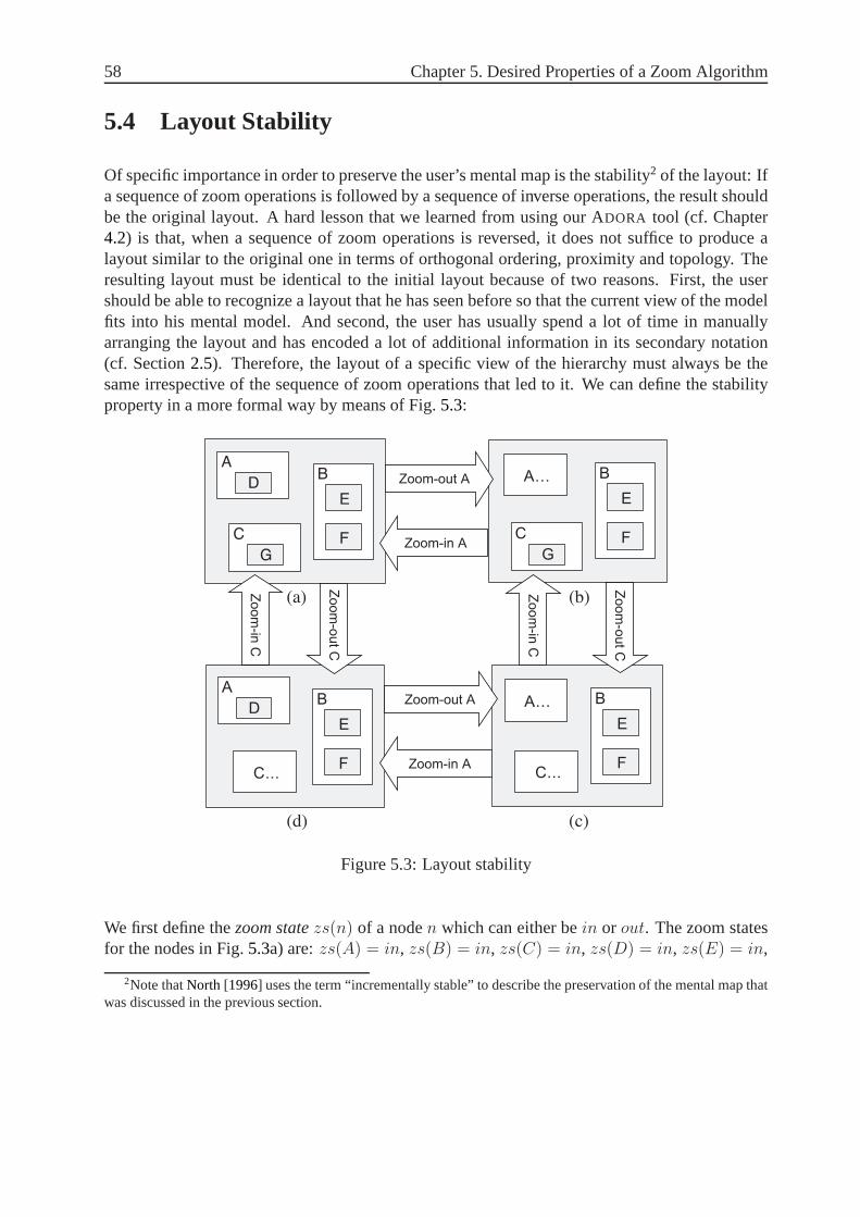
58 Chapter 5. Desired Properties of a Zoom Algorithm
5.4 Layout Stability
Of specific importance in order to preserve the user’s mentalmap is the stability2 of the layout: Ifa sequence of zoom operations is followed by a sequence of inverse operations, the result shouldbe the original layout. A hard lesson that we learned from using our ADORA tool (cf. Chapter4.2) is that, when a sequence of zoom operations is reversed, it does not suffice to produce alayout similar to the original one in terms of orthogonal ordering, proximity and topology. Theresulting layout must be identical to the initial layout because of two reasons. First, the usershould be able to recognize a layout that he has seen before sothat the current view of the modelfits into his mental model. And second, the user has usually spend a lot of time in manuallyarranging the layout and has encoded a lot of additional information in its secondary notation(cf. Section2.5). Therefore, the layout of a specific view of the hierarchy must always be thesame irrespective of the sequence of zoom operations that led to it. We can define the stabilityproperty in a more formal way by means of Fig.5.3:
D
A
E
F
B
G
C
A...
E
F
B
G
C
A...
E
F
B
C...
D
A
E
F
B
C...
(a) (b)
(d) (c)
Zoom-out A
Zoom-in A
Zoom-out A
Zoom-in A
Zoom
-in C
Zoom
-out C
Zoom
-out C
Zoom
-in C
Figure 5.3: Layout stability
We first define thezoom statezs(n) of a noden which can either bein or out. The zoom statesfor the nodes in Fig.5.3a) are:zs(A) = in, zs(B) = in, zs(C) = in, zs(D) = in, zs(E) = in,
2Note thatNorth [1996] uses the term “incrementally stable” to describe the preservation of the mental map thatwas discussed in the previous section.

5.5 Permit Editing Operations 59
zs(F ) = in andzs(G) = in. Note that the zoom state of notes that do not have any childrenand cannot switch their state is always set toin. The zoom state of nodeA changes in Fig.5.3b)to zs(A) = out because nodeA is zoomed-out while the zoom states of the other nodes remainunchanged. Furthermore, we define the zoom state of the modelmzs(Θ) as the set containingthe zoom states of all nodes, so that the model zoom statemzs(Θa) = zs(A) = in, zs(B) =in, zs(C) = in, zs(D) = in, zs(E) = in, zs(F ) = in, zs(G) = in is shown in Fig.5.3a).Nodes whose parent is in the zoom stateout can be omitted from the state definition, so that themodel zoom state of Fig.5.3c) is defined asmzs(Θc) = zs(A) = out, zs(B) = in, zs(C) =out, zs(E) = in, zs(F ) = in. The number of model zoom states (i.e., the model zoom statespace) can become quite large because it containsn2 states, wheren is the number of nodes thathave children and can therefore be zoomed.
A model zoom statemzs(Θ) describes a specific view on the hierarchy of the model (i.e.,whichnodes are currently visible because their parent node is zoomed-in or suppressed because theirparent is zoomed-out). The layout stability characteristic states now that there exists exactly onelayout for each model zoom statemzs(Θ). Any sequence of zoom operations that results ina specific model zoom state must also result in this specific layout. For example, zooming-outnodeA in Fig.5.3a) results in the layout of Fig.5.3b). Zooming-out nodeC and then zooming-inA produces the layouts of Fig.5.3c) and Fig.5.3d) respectively. If the next zoom operation isa zoom-in of nodeC then the layout must be identical to the initial layout of Fig. 5.3a). Thisproperty must hold even though the inverse zoom operations have not been performed in strictlyreverse order. This means that the zoom operations must be commutative (i.e., the order in whichthey are performed must not have any influence on the final layout).
5.5 Permit Editing Operations
Graphical models are manually and incrementally built by a modeler, so that the models arenot static but change and evolve over time. The possibility to directly manipulate the modelis one of the biggest advantages of computer-based modelingtools over paper-based modeling[Scaife and Rogers, 1996]. The technique that is used for their visualization must support manualmodifications of the model. A user may re-arrange the layout of a model or he may changethe model by adding or removing elements. This is not the casefor “pure” visualization orpresentation tools that are used in the reengineering field and show an existing structure (e.g., theprogram code) which is not modified anymore. Thus, we can distinguish between visualizationtools that show a static existing structure and graphical editors that are used to dynamically andincrementally build the structure. Since we want to use the zoom algorithm for graphical editors,it must permit editing operations (add, remove, move and resize nodes) and should try to preservethe modified layout as far as possible in subsequent zoom operations. The user must be able toedit the diagram regardless of the current view (i.e., the current zoom state) of the model becausehe is almost always working on an abstracted view (i.e., withsome of the nodes hidden) andalmost never on the fully expanded model.

60 Chapter 5. Desired Properties of a Zoom Algorithm
As the editing of models that use the nested box notation employs specific problems (cf. Chapter9), the zoom algorithm should support automatic layout expansion when an inserted node islarger than the empty space at the insertion point as well as automatic layout contraction whena node is removed. The existing layout should be maintained as far as possible in case of thisautomatic expansion and contraction in order to maintain the user’s mental map (cf. Section5.3).However, this is only possible to some extend because the stability property (cf. Section5.4) maynot hold anymore if the model has been edited between zoom operations. The need to supportediting operations renders approaches which simply store the layout of all zoom states in order toreconstruct the layout impossible (because changing one layout may change all stored layouts).
5.6 Runtime
Zooming is part of an interactive viewing, navigating and editing process. Hence, the zoomingoperations have to be performed with no remarkable delay even for big models [Bartram et al.,1995; Leung and Apperley, 1994]. This results in an upper limit on the runtime (and possiblyspace) complexity of the zoom algorithm: Algorithms that have a quadratic or exponential run-time with respect to the number of nodes in the model are not usable. For example, the runtime isa problem for the graphically distorting techniques (cf. Section3.1.4) because they are inherentlycomplicated in their implementation and some of them require a significant amount of systemtime to generate a new image [Leung and Apperley, 1994]. Furthermore, the property that thedisplay of a new layout after a zoom operation should be immediate makes it hard to apply tech-niques that try to detect overlapping nodes and remove the overlaps because the detection usuallyimplies an exponential runtime because each node has to be checked against each other node.
5.7 Multiple Focal Points
It is often desirable to view multiple areas of a model in detail simultaneously. The zoom algo-rithm should therefore support multiple focal points [Bartram et al., 1995; Furnas, 1986; Leungand Apperley, 1994; Shoemaker and Gutwin, 2007]. This property is of special importance forrelational data where the details of one entity can often notbe fully understood without seeingthe details of related entities. For example, in the case of models of software systems it is of-ten necessary to examine several subsystems or components and their mutual interconnectionsconcurrently [Storey et al., 1997a]. This also implies that the user must always have full controlover all focal points (i.e., he can set or remove a focal pointto/from any node in the model all thetime). Thus, the system must not close or decrease the size ofnodes besides the focal point auto-matically if the focus changes. Nodes always have to be opened and closed explicitly by the user.Closing or resizing nodes automatically may also result in abunch of layout operations after aminimal change of the focus by the user. Additionally, hiding nodes automatically if their sizefalls below a defined threshold my be quite dangerous as it is not obvious for the user whether

5.8 Smooth Transitions 61
the node does not exist at all or is just hidden at the moment. The price that has to be paid forleaving the user in full control is that the visual complexity [Li et al., 2005] of the diagram isnot reduced automatically and an increase in the interaction overhead (cf. Section5.9). Thistrade-off between how much influence the user should have andhow much is done automaticallyby the tool emerges in almost all computer supported tasks and can usually not be solved easily.For example, in an experimental comparisons between a linear, an overview+detail and a fisheyeinterface for reading text documents [Hornbæk and Frøkjær, 2003] the subjects commented thatthey did not like to depend on an algorithm to determine whichparts of the document should bereadable at the moment
5.8 Smooth Transitions
The transition between the current layout and the new layoutthat results from a zoom operationcan result in the user being suddenly “lost in the diagram”. The user usually needs several sec-onds to re-assimilate to the new layout. Therefore, the transition between the layouts should besmooth to enhance the continuity [Bartram et al., 1995; Noik, 1994]. Animation provides a wayto do so by expressing the causality that led to the new layout[Ware, 2004]. An interactive an-imation shifts some of the user’s cognitive load to the perceptual system because the perceptualphenomenon of object constancy enables the user to track structural relationships without think-ing about them [Robertson et al., 1991]. The changes in the layout are tracked by the perceptualsystem so that no re-assimilation is needed afterwards. Thetechnique of interactive animationhas been employed by the CAD (computer-aided design) field for years by animating the rotationof complex structures. Animated transitions offer a way to preserve the mental map while adjust-ing the layout [Bederson and Boltman, 1999; Bridgeman and Tamassia, 2000] and are thereforea lot more than just “eye candy” to increase the visual attractiveness.
Empirical results indicate that animation indeed aids comprehension [Bederson and Boltman,1999; Gonzalez, 1996; Klein and Bederson, 2005], but there is no evidence that it also aids taskperformance time [Chui and Dillon, 1997; Donskoy and Kaptelinin, 1997]. The recommendedspeed for transitions in animated zooming varies between 0.3 and 1.0 seconds, depending onthe application domain and the difference between the initial and final layout [Bederson andBoltman, 1999; Card et al., 1991; Klein and Bederson, 2005].
5.9 Small Interaction Overhead
The introduction of a fisheye zoom algorithm into a modeling tool lets the user interactivelyexplore the model and generate different views that are bestsuited for his current task. Theinteraction overhead that is required to achieve this effects should be as small as possible andthe user should remain in control all the time [Bartram et al., 1995]. The interaction can be
62 Chapter 5. Desired Properties of a Zoom Algorithm
greatly simplified if it is possible to interact directly with the model elements (e.g., by clickingon a node to zoom-in or out) instead of using control elementsthat are only indirectly connectedto the model elements [Scaife and Rogers, 1996]. A user command should then immediatelylead to a feedback by the system. Additionally, the user mustknow all the time where he isin the diagram and where he can go from there (i.e., the user should be aware of all possiblenavigation paths from the current diagram [Kim et al., 2000]) to effectively interact with thediagram. An example of a problem in the interaction between the user and the model can befound in the graphically distorting techniques (cf. Section 3.1.4): The nonlinear magnificationmakes the target acquisition cumbersome because objects appear to move away as the focal pointapproaches them [Gutwin, 2002].
5.10 Minimal Node Size
Some of the focus + context techniques (cf. Section3.1.4) take the metaphor literally and try toshow all the context all the time (i.e., they always show all nodes of the diagram on the screen,though some of them may be visible in an abstracted form). They tighten the property of disjointnodes (cf. Section5.2) by stating that “information, whether in a detailed or summary view,should never be occluded” [Bartram et al., 1995], which also makes viewports and scrollbarsinappropriate because they do not show the elements that layoutside the currently visible areaof the screen. The main problem with these approaches is thatindividual model elements canbecome very small if big models (as they often occur for software systems) have to be shown ontoday’s (small) display screens. This makes the interaction cumbersome because of two reasons:First, it can become difficult to hit a small node during the target acquisition (e.g., while clickingon a node to zoom it). And second, the text labels that are usedto name nodes and links are notreadable anymore if their size becomes too small. Therefore, the size of the nodes must not fallbelow a defined threshold.
63
CHAPTER 6
Existing Fisheye Zoom Techniques
Different fields face the same problem of showing large information spaces on small screens, sothat a variety of techniques to manage the complexity of diagrams have emerged (see e.g. [Noik,1994; Spence, 2007, chap. 4] for an overview). This chapter shortly describes the techniquesthat are most important in the context of graphical models and asseses them against the criteriaof Chapter5. The discussion has a strong bias on the weaknesses of the presented approaches toshow why none of them has all the desired properties presented in the last chapter.
All techniques presented in this chapter combine suppression with global distortion (cf. Section3.3.4) but they originate from different fields: The force-scan algorithm (Section6.1) has itsorigins in the field of automatic graph drawing. SHriMP (Section 6.2) was developed to visu-alize large software structures in the reengineering field.The algorithm of Berner (Section6.3)has been used for the previous version of the ADORA tool and the Continuous Zoom (Section6.4) stems from the human-computer interaction field where it has been developed for the userinterface of control systems.
Layout Manipulation and Geometric Projection
The presented approaches can be broadly divided in two categories: On the one hand, those thatstore the model internally in a “fixed canonical coordinate system” [Furnas and Bederson, 1995](or “normal view” [Noik, 1994]) which is the fully expanded model with all nodes shown infull size and use geometric projections (e.g., scale factors) during the rendering process. Thetechniques that belong to this category are the Graphical Fisheye Views presented in Section

64 Chapter 6. Existing Fisheye Zoom Techniques
3.1.4and the Continuous Zoom. The fixed coordinate system makes itdifficult to permit editingoperations independent of the current state of the layout. On the other hand are those techniquesthat store and directly manipulate the current layout, suchas the force-scan algorithm, SHriMPand Berner’s algorithm. These techniques have only one representation of the model, the onethat is currently shown.
6.1 The Force-Scan Algorithm
The force-scan algorithm [Misue et al., 1995] uses the basic concept underlying the “springalgorithms” [Eades, 1984] which are used for the automatic graph drawing (cf. Section2.3.1) toresolve overlaps between nodes. The main idea is to use a “force” fuv between two nodesu andv that pushes the two away from each other if they overlap. Fig.6.1 illustrates the force-scanalgorithm:
Pu = (x
u, y
u) P
u = (x
u, y
u)
Pv = (x
v, y
v)
R = (x, y)
Figure 6.1: The force-scan algorithm
The direction of the forcefuv is along the line that connects the centers of the two nodesPu =(xu, yu) andPv = (xv, yv). The magnitude offuv is set to the difference between the “actualdistance”duv and the “desirable distance”kuv between the two nodes. The actual distance is theEuclidean distance between the two node centersPu andPv:
duv =√
(xu − xv)2 + (yu − yv)2 (6.1)
The desirable distance is defined as follows:R = (x, y) is the first point along the line thatconnects the two node centersPu andPv for which either
|x− xu| ≥wu + wv
2or |y − yu| ≥
hu + hv
2(6.2)
holds and wherewu is the width of nodeu andhu is the height of nodeu. The pointR is thefirst point along the line connectingPu andPv for which nodeu with centerPu is disjoint from

6.2 SHriMP 65
nodev with centerR. The desirable distancekuv is then the Euclidean distance betweenPu andR. The magnitude of the forcefuv becomeskuv − duv if the two nodesu andv overlap:
fuv = max(0, kuv − duv)luv (6.3)
whereluv is a unit vector in the direction frompu to pv. A constant valueg can be added tokuvto force a gap of sizeg between the nodes. Misue et al. call this approach thepush force-scanalgorithmbecause the force can according to formula6.3 only be positive which “pushes” thenodes away. Additionally, they propose thepush-pull force-scan algorithmwhich allows bothpositive and negative forces:
fuv = (kuv − duv)luv (6.4)
The push-pull force-scan algorithm additionally compactsdiagrams which are too sparsely spreadout while preserving the general shape of the diagram.
Discussion
The biggest drawback of the force-scan algorithm is that thenodes in its output are not alwaysdisjoint. The algorithm has to be repeated until all nodes are disjoint. Therefore, a complexlayout can result in a lot of runs of the algorithm. Furthermore, the force-scan algorithm cannotguarantee the stability of the layout because of its heuristic nature: The algorithm calculatesall forces and “lets the system go” so that an equilibrium (minimum energy) is reached [Eades,1984]. However, this equilibrium does not look the same all the time because a different localoptimum can be reached. A similar approach is the OrthogonalDynamic Natural Length Spring(ODNLS) algorithm byLi et al. [2005].
6.2 SHriMP
The SHriMP (Simple HierarchicalMulti-Perspective) visualization technique has been devel-oped byStorey and Müller[1995] to create fisheye views of nested graphs. The technique hasits roots in the reengineering field where large existing software systems have to be visualizedon small computer screens to explore their structure and browse the source code.
The concept behind SHriMP tries to evenly distribute the distortion throughout the entire graphby uniformly scaling the nodes outside the focal point(s) toavoid too much distortion in someparts of the diagram (as it happens with the Graphical Fisheye Views of Section3.1.4). Nodesin the graph uniformly give up screen space to allow a node of interest to grow. A node growsby pushing its sibling nodes outward. All nodes are then scaled around the center of the screen
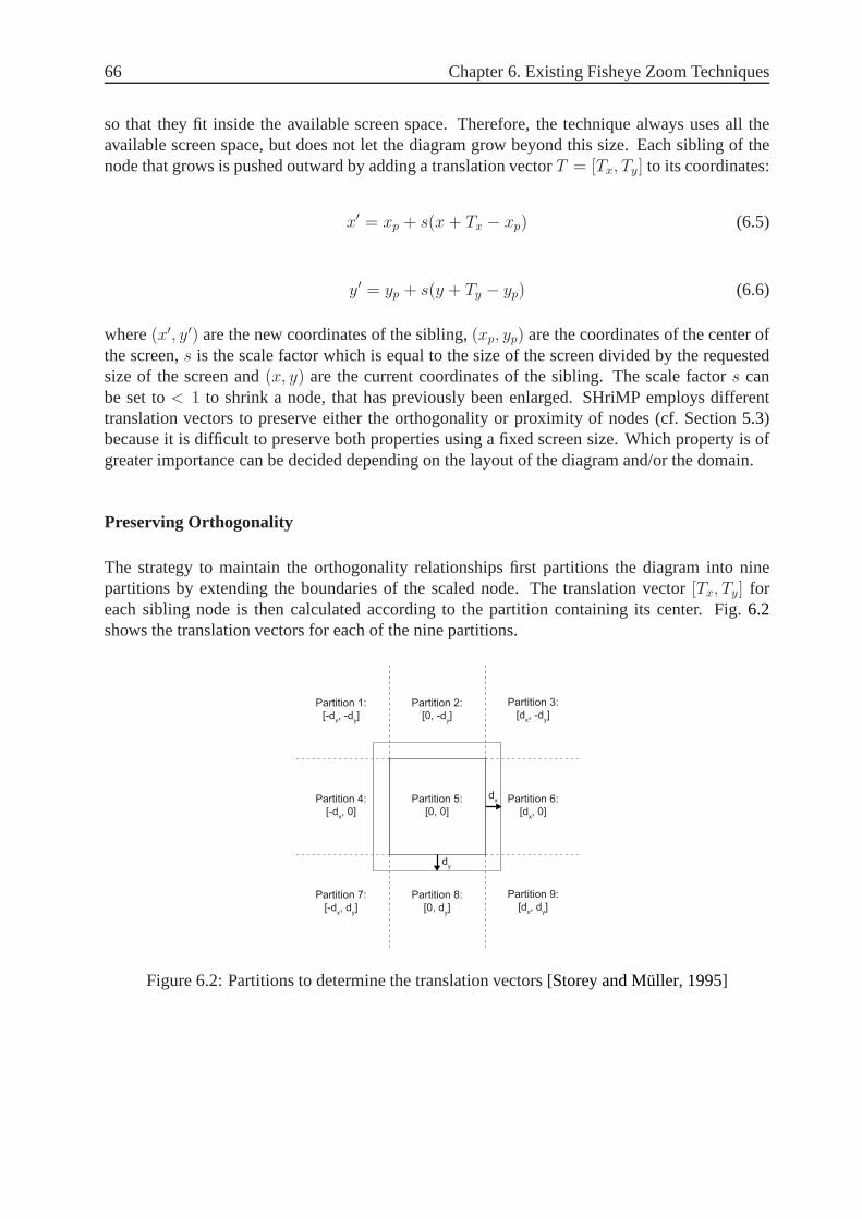
66 Chapter 6. Existing Fisheye Zoom Techniques
so that they fit inside the available screen space. Therefore, the technique always uses all theavailable screen space, but does not let the diagram grow beyond this size. Each sibling of thenode that grows is pushed outward by adding a translation vector T = [Tx, Ty] to its coordinates:
x′ = xp + s(x+ Tx − xp) (6.5)
y′ = yp + s(y + Ty − yp) (6.6)
where(x′, y′) are the new coordinates of the sibling,(xp, yp) are the coordinates of the center ofthe screen,s is the scale factor which is equal to the size of the screen divided by the requestedsize of the screen and(x, y) are the current coordinates of the sibling. The scale factors canbe set to< 1 to shrink a node, that has previously been enlarged. SHriMP employs differenttranslation vectors to preserve either the orthogonality or proximity of nodes (cf. Section5.3)because it is difficult to preserve both properties using a fixed screen size. Which property is ofgreater importance can be decided depending on the layout ofthe diagram and/or the domain.
Preserving Orthogonality
The strategy to maintain the orthogonality relationships first partitions the diagram into ninepartitions by extending the boundaries of the scaled node. The translation vector[Tx, Ty] foreach sibling node is then calculated according to the partition containing its center. Fig.6.2shows the translation vectors for each of the nine partitions.
Partition 3:
[dx, -d
y]
Partition 2:
[0, -dy]
Partition 1:
[-dx, -d
y]
Partition 4:
[-dx, 0]
Partition 7:
[-dx, d
y]
Partition 5:
[0, 0]
Partition 6:
[dx, 0]
Partition 8:
[0, dy]
Partition 9:
[dx, d
y]
dx
dy
Figure 6.2: Partitions to determine the translation vectors [Storey and Müller, 1995]

6.2 SHriMP 67
For example, a node whose center lies in partition 3 is moved by the translation vectorT =[dx,−dy], wheredx anddy are the differences between the new and current width and heightof the scaled node. All sibling nodes above and below the scaled node are moved upwards anddownwards by the same amount while the nodes on the right and left side are moved right andleft, which preserves the vertical and horizontal orthogonality relationships (cf. Section5.3).
Preserving Proximity
Groups or clusters of nodes that depict certain relationships in the diagram are maintained bypreserving the proximity relationships (cf. Section5.3). SHriMP preserves this property by con-straining each sibling node to stay on the line connecting its center and the center of the nodebeing scaled. The resized node pushes the sibling node outwards along this line. Fig.6.3showsthe calculation of the translation vector for nodeB if nodeA grows.
(xa, y
a)
(xb, y
b)
dx
dy
µ
A
B
µ
Figure 6.3: Proximity preservation strategy [Storey and Müller, 1995]
The direction of the translation vector forB is equal to the direction of the line that connects thecenter ofB (xb, yb) with the center of the scaled nodeA (xa, ya). The magnitude of this vectorµ is calculated from the differences between the new width andheight of the scaled nodeA andits previous width and height:
µ =√
d2x + d2y (6.7)
The magnitudeµ is the same for all sibling nodes and needs to be calculated only once. The com-ponents of the translation vectorT = [Tx, Ty] are then calculated by multiplying the magnitudewith the direction of the vector:
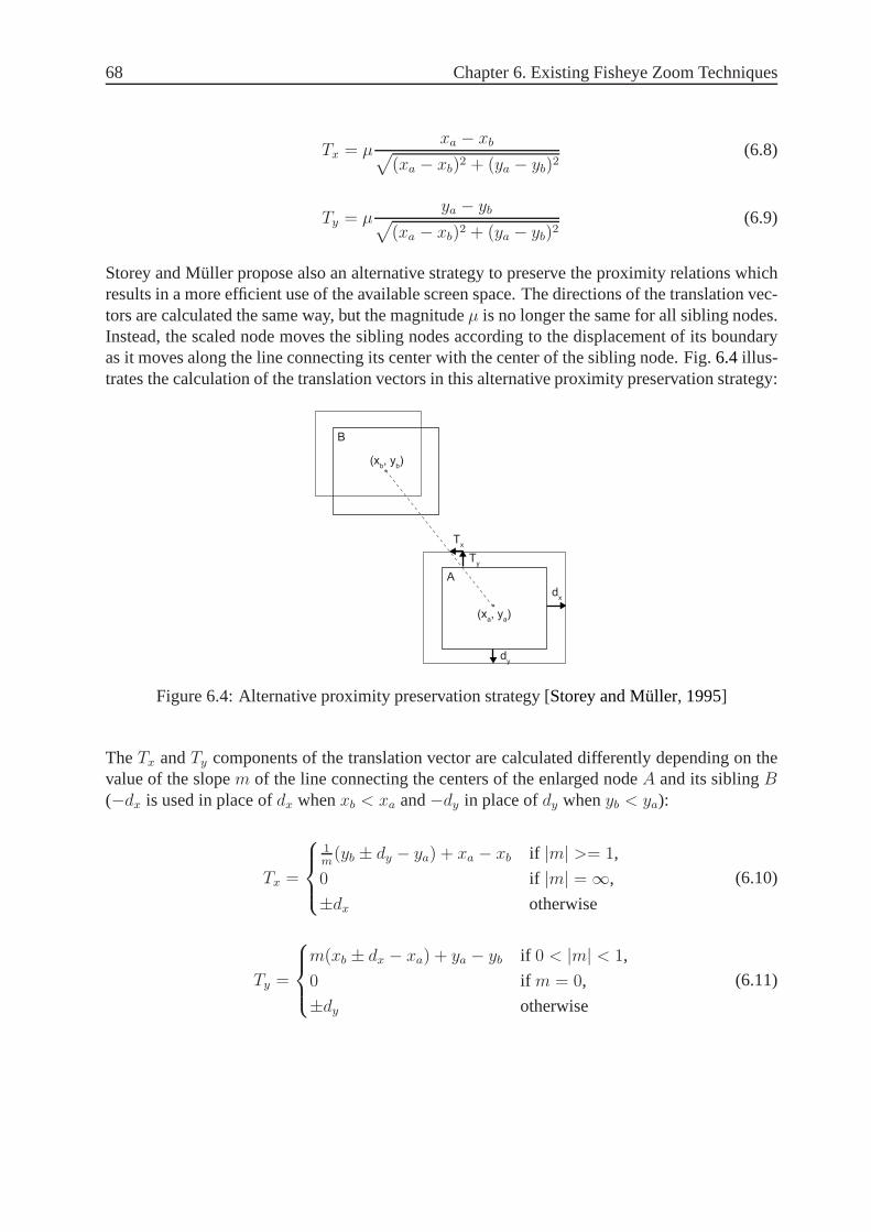
68 Chapter 6. Existing Fisheye Zoom Techniques
Tx = µxa − xb
√
(xa − xb)2 + (ya − yb)2(6.8)
Ty = µya − yb
√
(xa − xb)2 + (ya − yb)2(6.9)
Storey and Müller propose also an alternative strategy to preserve the proximity relations whichresults in a more efficient use of the available screen space.The directions of the translation vec-tors are calculated the same way, but the magnitudeµ is no longer the same for all sibling nodes.Instead, the scaled node moves the sibling nodes according to the displacement of its boundaryas it moves along the line connecting its center with the center of the sibling node. Fig.6.4illus-trates the calculation of the translation vectors in this alternative proximity preservation strategy:
(xb, y
b)
(xa, y
a)
A
B
dx
dy
Tx
Ty
Figure 6.4: Alternative proximity preservation strategy [Storey and Müller, 1995]
TheTx andTy components of the translation vector are calculated differently depending on thevalue of the slopem of the line connecting the centers of the enlarged nodeA and its siblingB(−dx is used in place ofdx whenxb < xa and−dy in place ofdy whenyb < ya):
Tx =
1
m(yb ± dy − ya) + xa − xb if |m| >= 1,
0 if |m| = ∞,
±dx otherwise
(6.10)
Ty =
m(xb ± dx − xa) + ya − yb if 0 < |m| < 1,
0 if m = 0,
±dy otherwise
(6.11)
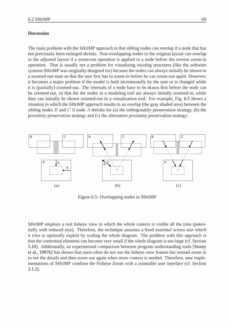
6.2 SHriMP 69
Discussion
The main problem with the SHriMP approach is that sibling nodes can overlap if a node that hasnot previously been enlarged shrinks. Non-overlapping nodes in the original layout can overlapin the adjusted layout if a zoom-out operation is applied to anode before the inverse zoom-inoperation. That is usually not a problem for visualizing existing structures (like the softwaresystems SHriMP was originally designed for) because the nodes can always initially be shown ina zoomed-out state so that the user first has to zoom-in beforehe can zoom-out again. However,it becomes a major problem if the model is built incrementally by the user or is changed whileit is (partially) zoomed-out. The internals of a node have tobe drawn first before the node canbe zoomed-out, so that the the nodes in a modeling tool are always initially zoomed-in, whilethey can initially be shown zoomed-out in a visualization tool. For example, Fig.6.5 shows asituation in which the SHriMP approach results in an overlap(the gray shaded area) between thesibling nodesB andC if nodeA shrinks for (a) the orthogonality preservation strategy, (b) theproximity preservation strategy and (c) the alternative proximity preservation strategy:
dx
dy
B C
A
B C
Aµ
B C
A
(a) (b) (c)
Figure 6.5: Overlapping nodes in SHriMP
SHriMP employs a real fisheye view in which the whole context is visible all the time (poten-tially with reduced size). Therefore, the technique assumes a fixed maximal screen size whichit tries to optimally exploit by scaling the whole diagram. The problem with this approach isthat the contextual elements can become very small if the whole diagram is too large (cf. Section5.10). Additionally, an experimental comparison between program understanding tools [Storeyet al., 1997b] has shown that users often do not use the fisheye view featurebut instead zoom into see the details and then zoom out again when more context isneeded. Therefore, new imple-mentations of SHriMP combine the Fisheye Zoom with a zoomable user interface (cf. Section3.1.2).

70 Chapter 6. Existing Fisheye Zoom Techniques
6.3 Berner
The zoom algorithm proposed by Berner [Berner, 2002; Berner et al., 1998] uses translationvectors to move sibling nodes in a very similar way as SHriMP does. However, it combines twoof SHriMP’s strategies: the orthogonality and the alternative proximity preservation. Fig.6.6illustrates how the translation vectors are calculated in Berner’s approach:
W E
S
A
B C
dx
dy
N NE: [dx, -d
y]
SE: [dx, d
y]
NW: [-dx, -d
y]
SW: [-dx, d
y]
Figure 6.6: Calculation of the translation vectors in Berner’s algorithm [Berner, 2002]
The nodes whose center lies in one of the corner partitions (NW, NE, SW and SE) are handledthe same way as in SHriMP’s orthogonality preservation strategy. Therefore, nodeC is movedby the two vectorsdx and−dy. Nodes whose center is in one of the other partitions (N, S, E andW) are moved by the translation vectors as they have been calculated by the alternative proximitypreservation strategy of SHriMP. The scaled nodeA moves the sibling nodeB according to thedisplacement of its boundary as it moves along the line connecting the centers ofA andB.
Discussion
Berner uses a hybrid strategy to better exploit the available space in the diagram. The algorithmshares the limitation of SHriMP that it cannot avoid overlapping nodes if a node is zoomed-outwithout previously being zoomed-in. However, Berner’s approach can also not guarantee thatthe zoom-in operations produce an overlapping free layout [Marty, 2002]. Fig. 6.7illustrates theproblem: SiblingsB andC have to be moved away asA grows to sizeA′. The translation vectorof nodeC is [dx,−dy] because the node’s center lies in the corner partitionNE. The center ofnodeB lies in the top partitionN and its translation vector is therefore calculated according toformulas6.10and6.11.

6.4 The Continuous Zoom 71
A’
B’ C’
A
B C
Figure 6.7: Overlapping nodes in Berner’s algorithm [Marty, 2002]
NodesB′ andC ′ overlap in the gray shaded area of the adjusted layout because the differentlycalculated translation vectors move the nodes closer together. Berner proposes to detect and thenautomatically resolve this node occlusions. However, the detection can be very costly (cf. Section5.6) and moving nodes to resolve one occlusion can easily resultin new occlusions. Additionally,an automatic occlusion resolution can destroy the secondary notation and the user’s mental map.
The basic problem with any technique that uses translation vectors to move the sibling nodes isthat it takes only the geometric relations between the zoomed node and its siblings into accountbut not the relations among these siblings. An independent translation vector is calculated foreach sibling node and the node is then moved in isolation without taking surrounding nodes intoaccount. This often results in overlapping nodes.
6.4 The Continuous Zoom
The Continuous Zoom of Bartram et al. [Bartram et al., 1995; Dill et al., 1994] (and its prede-cessor, the Variable Zoom [Schaffer et al., 1996]) allows the user to control the amount of detailin different areas of the model by opening and closing “clusters” (i.e., nodes that contain othernodes) which toggles the visibility of the contents of the node and allocates more or less spaceto it. The user can, in addition to this automatic resizing, freely enlarge or reduce the size ofany node in the diagram. The Continuous Zoom is presented in greater detail here because ourown zoom algorithm presented in Chapter7 builds on the basic ideas of the Continuous Zoom,namely an interval structure and the concept of scaling interval sizes.

72 Chapter 6. Existing Fisheye Zoom Techniques
The zoom algorithm combines the initial layout (the so called “normal geometry”) with a setof scale factors to produce the “zoomed geometry”. The normal geometry is constant whilethe scale factor for each node is determined by the user. The scale factor of a node whose sizeremains the same is set to1.0. The boundaries of the nodes are first independently projected ontothe x and y axes, which results in a set of non-overlapping intervals (represented by the dottedlines in Fig.6.8). A scale factor is then calculated for each horizontal and vertical interval. Thescale factor of an interval corresponding to a node projection is the scale factor of this node.The algorithm takes the maximum scale factor of all projected nodes if two or more projectionsoverlap (asA andB on the x axis in Fig.6.8). The scale factor for gap intervals (i.e., intervals thatare not a projection of any node) is set to the maximum scale factor of its neighboring intervals.
C
B
A
5
2530
50
70
80
90
15 20 45 95 110 140 150
Figure 6.8: Normal geometry of the Continuous Zoom
The algorithm then uses a budgeting process to distribute the available space among nodes. Itsums the amount of space that is requested by each node up and then distributes a fixed overallspace budget (the display size) according to the size of eachrequest. The total amount of spacerequested by all nodes inside a cluster in x directionXreq is calculated according to6.12, wherexi is the normal length of theith interval (the normal length of an interval is the interval’slengthin the normal geometry) andsi is the interval’s scale factor.
Xreq =∑
i
xisi (6.12)
As an example, lets assume that the size of nodeA in Fig. 6.8 is scaled down by the factor0.5.The accumulated normal lengths of the horizontal and vertical intervals in Fig.6.8 are shownby the numbers on the boundaries of the intervals. The scale factor for nodesB andC is 1.0,because their size remains the same. Thus, the total space that is requested in the x direction is:

6.4 The Continuous Zoom 73
Xreq = 15 ∗ 1 + 5 ∗ 1 + 25 ∗ 1 + 50 ∗ 0.5 + 15 ∗ 1 + 30 ∗ 1 + 10 ∗ 1 = 125 (6.13)
The third horizontal interval (the one with the normal length of 25) is scaled by the factor1.0because nodesA andB are both projected to this interval and the zoom algorithm takes thebigger of the two scale factors which is in the example the oneof B. The size of a node must beadjusted if the size of at least one of its children changes. Therefore, the scale factor of a parentnode is “inherited” from its children’s scale factors:
Sp =Xreq
Xp
(6.14)
WhereSp is the scale factor andXp the normal width of the parent node. The space request ofeach node is propagated upwards until the root node is reached. The size of the root node is fixed(limited by the screen size). The parent node ofA, B andC in Fig. 6.8 is the root node so thatits scale factor in x direction becomes:
Sroot =125
150= 0.83 (6.15)
The normal width of the root node in Fig.6.8in x direction of 150 is the sum of all the horizontalintervals’ normal lengths. The scaleSi of each interval in the hierarchy is divided by the scalefactor of the root nodeSroot, so that the size of the whole diagram remains constant. The zoomedlengthx∗
i of an interval is then the normal lengthxi of the interval multiplied by this modifiedscale factor:
x∗
i = xi
Si
Sroot
(6.16)
For the first horizontal interval in Fig.6.8(for which the normal length is 15 and the scale factor1.0) this becomes:
x∗
1= 15
1.0
0.83= 18 (6.17)
The length of the horizontal and vertical intervals containing a node constitute the total spaceavailable to that node (the so called zoom hole). The final size of a node has to be calculatedseparately because the size of the node may differ from its zoom hole (because of differences inthe scale factors):
L∗
k = Lk
Sk
Sroot
(6.18)

74 Chapter 6. Existing Fisheye Zoom Techniques
WhereL∗
k is the zoomed width,Lk the normal width andSk the scale factor of nodek. Thisresults in the new width of nodeA:
L∗
A = 750.5
0.83= 45.18 (6.19)
The nodes are repositioned according to the location of their center points inside the correspond-ing interval. The aspect ratio of the nodes may change because the zoomed width and height arecalculated separately. The smaller of the two scale factorscan be applied in both directions toheld the aspect ratio constant (which may in turn result in aninefficient use of space). Applyingthe just described algorithm accordingly to the horizontaland vertical intervals of Fig.6.8resultsin the final situation shown in Fig.6.9. Note that the decrease ofA’s size results in an increaseof the size ofB andC. The zoom holes of the nodes are depicted by the gray shaded areas in thefigure.
C’
B’
A’
6
30
36
48
72
78
90
18 24 54 84 102 138 150
Figure 6.9: Node A has been scaled down by factor 0.5
Automatic Node Sizing
The Continuous Zoom relies on the user in deciding on the sizeof a node. However, early usertesting indicated a desire for more optimal sizing in which the node opens to its maximum sizewithout any extra manipulation. Thus, the focus of the approach has shifted over time towardsreducing the amount of size manipulations for the user with the ultimate goal of automating thenode sizing. As a possible solution,Bartram et al.[1995] suggest to use the Degree of Interest(cf. Section3.3.3) for the automatic node sizing. The DOIs are dynamically calculated based ona node’s a priori importance, its current state (e.g., normal operation or alarm state in the case of

6.4 The Continuous Zoom 75
a control system) and its proximity to interesting nodes (i.e., nodes with a high DOI). As a result,neighbors of interesting nodes get more space than nodes that are further away, which results inthe fisheye effect.
Discussion
The basic assumption of the Continuous Zoom that the size of the diagram (which is determinedby the available display space) remains fixed, results in a global behavior of the zoom algorithm:changing the scale factor of just one nodes changes the size of all nodes (as can easily be seenby comparing Fig.6.8 and Fig.6.9). This global nature can have a negative influence on theuser’s mental map as shown by some early user reactions [Dill et al., 1994]: “Some users foundthe resulting motion in peripheral parts of the display to bedistracting when they were tryingto focus or setting the size of a particular node. Furthermore, after setting the size of one node,it was annoying to have it change as a result of resizing another node somewhere else.” Suchinterdependencies between node sizes is inevitable because the diagram has a fixed size.
An additional problem that results from the assumption thatthe screen has a fixed size and isalways completely visible is the fact that most graphical models are just too big (or the screenstoo small) so that they cannot be completely shown at once on ascreen even when an fisheyetechnique is applied (cf. Section5.10). This problem emerges with all “In-Situ Magnification”techniques [Berner, 2002] which assume a fixed diagram size such as SHriMP (cf. Section6.2)or the distortion-oriented techniques (cf. Section3.1.4).
And finally, the basic geometric projection of the Continuous Zoom that combines the fixed nor-mal geometry and the scale factors to generate a geometric projection, the zoomed geometry,makes it difficult to permit editing operations independentof the current state of the scaled ge-ometry. While the editing takes place on the zoomed geometry, the changes have to be appliedback through the geometric transformations onto the normalgeometry.


77
CHAPTER 7
Zoom Algorithm
The purpose of a zoom algorithm is to produce a new layout if the size of a node changes becauseits inner structure is hidden or shown. It takes an existing layout (i.e., the position and size of aset of non-overlapping nodes) as well as a new size for an existing nodeη as input and calculatesa new layout. The size ofη is updated to the new size and the position of the siblings is adjustedto the new size ofη. The zoomed-in or zoomed-out nodeη (or one of its siblings) pushes theboundaries of its parent outward or pulls them inward, respectively. The parent in turn pushesor pulls its siblings, which is done recursively until the root node is reached. Thus, the zoomalgorithm is applied recursively on all the direct or indirect parents ofη.
The presented algorithm works on an interval structure and employs the concept of scaling inter-val sizes1 and is therefore similar to the Continuous Zoom byBartram et al.[1995] (cf. Section6.4). However, our approach does not assume a fixed basic layout,does not globally scale thewhole model and uses different scaling functions. The improved zoom algorithm has all proper-ties described in Chapter5, thus overcoming the limitations of the other approaches presented inChapter6. We assume a layout with rectangular representations of thenodes. However, this isno limitation as the boundaries of nodes with arbitrary shape can be represented by a rectangle.Parts of the algorithm have already been published in [Reinhard et al., 2007, 2008].
1This idea goes back to the very early focus+context techniques like the Bifocal Display [Spence and Apperley,1982] and the Rubber Sheet [Sarkar et al., 1993].
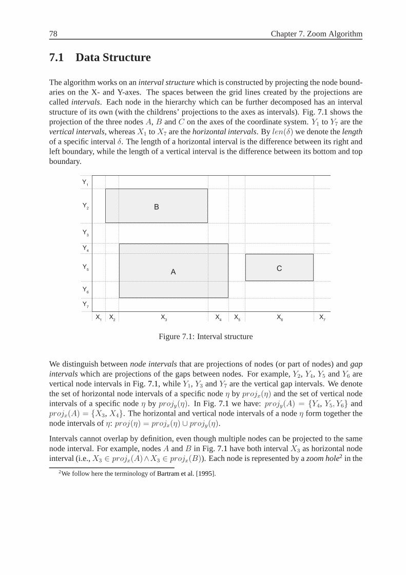
78 Chapter 7. Zoom Algorithm
7.1 Data Structure
The algorithm works on aninterval structurewhich is constructed by projecting the node bound-aries on the X- and Y-axes. The spaces between the grid lines created by the projections arecalled intervals. Each node in the hierarchy which can be further decomposed has an intervalstructure of its own (with the childrens’ projections to theaxes as intervals). Fig.7.1shows theprojection of the three nodesA, B andC on the axes of the coordinate system.Y1 to Y7 are thevertical intervals, whereasX1 toX7 are thehorizontal intervals. By len(δ) we denote thelengthof a specific intervalδ. The length of a horizontal interval is the difference between its right andleft boundary, while the length of a vertical interval is thedifference between its bottom and topboundary.
A
B
C
X2
X3
X4
X5
X6
X7
X1
Y1
Y2
Y3
Y4
Y5
Y6
Y7
Figure 7.1: Interval structure
We distinguish betweennode intervalsthat are projections of nodes (or part of nodes) andgapintervalswhich are projections of the gaps between nodes. For example, Y2, Y4, Y5 andY6 arevertical node intervals in Fig.7.1, while Y1, Y3 andY7 are the vertical gap intervals. We denotethe set of horizontal node intervals of a specific nodeη by projx(η) and the set of vertical nodeintervals of a specific nodeη by projy(η). In Fig. 7.1 we have:projy(A) = Y4, Y5, Y6 andprojx(A) = X3, X4. The horizontal and vertical node intervals of a nodeη form together thenode intervals ofη: proj(η) = projx(η) ∪ projy(η).
Intervals cannot overlap by definition, even though multiple nodes can be projected to the samenode interval. For example, nodesA andB in Fig. 7.1have both intervalX3 as horizontal nodeinterval (i.e.,X3 ∈ projx(A)∧X3 ∈ projx(B)). Each node is represented by azoom hole2 in the
2We follow here the terminology ofBartram et al.[1995].

7.1 Data Structure 79
interval structure. The zoom holes of nodesA, B andC are shown by the gray shaded rectanglesin Fig. 7.1. The width of a zoom hole is equal to the accumulated length ofthe node’s horizontalnode intervals, while its height is equal to the accumulatedlength of the node’s vertical nodeintervals.
The order of the vertical and horizontal intervals is alwayspreserved if a zoom operation is ap-plied to the interval structure even though the lengths of the intervals may change. This propertyis important to guarantee an overlapping-free layout aftera zoom operation (cf. Section5.2).
Construction of the Interval Structure
The interval structure of a node is incrementally build by adding nodes when they are insertedinto the structure’s parent node. The horizontal and vertical intervals are completely independentso that they are also updated separately when a node is inserted. The algorithm to adjust thehorizontal intervals in the structure once a new node is inserted works as follows (the verticalintervals are adjusted accordingly):
1. The intervalδleft that contains the left boundary of the node is identified. This can beachieved by a sequential or binary search since the intervals are stored in a sorted sequentiallist.
2. Intervalδleft is split at the position of the node’s left boundary (if this boundary lies withinthe interval). The interval that has been newly created by this split is added to the listcontaining all horizontal intervals of the structure andδleft is set to this new interval.
3. The intervalδright that contains the right boundary of the node is identified.
4. A reference to the zoom hole of the inserted node is added toall intervals between the leftδleft (inclusive) and rightδright (exclusive) interval. Additionally, a reference to each ofthese intervals is added to the horizontal intervals of the zoom hole of the node.
5. The right intervalδright is split at the position of the node’s right boundary (if thisboundarylies within the interval). The interval that has been newly created by this split is added tothe list containing the horizontal intervals of the structure.
6. A reference to the zoom hole of the inserted node is added tothe right intervalδright and areference to the right intervalδright is added to the zoom hole of the inserted node.
Removing a Node from the Interval Structure
The horizontal and vertical intervals of an interval structure have to be adjusted if a child isremoved from a node so that the interval structure still reflects the internal structure of this parentnode. The horizontal and vertical intervals are managed independently so that they can also be
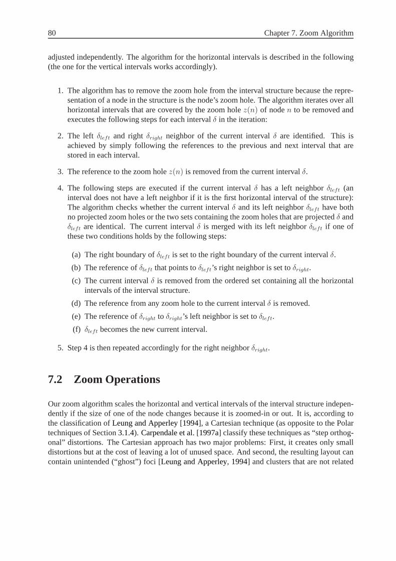
80 Chapter 7. Zoom Algorithm
adjusted independently. The algorithm for the horizontal intervals is described in the following(the one for the vertical intervals works accordingly).
1. The algorithm has to remove the zoom hole from the intervalstructure because the repre-sentation of a node in the structure is the node’s zoom hole. The algorithm iterates over allhorizontal intervals that are covered by the zoom holez(n) of noden to be removed andexecutes the following steps for each intervalδ in the iteration:
2. The left δleft and rightδright neighbor of the current intervalδ are identified. This isachieved by simply following the references to the previousand next interval that arestored in each interval.
3. The reference to the zoom holez(n) is removed from the current intervalδ.
4. The following steps are executed if the current intervalδ has a left neighborδleft (aninterval does not have a left neighbor if it is the first horizontal interval of the structure):The algorithm checks whether the current intervalδ and its left neighborδleft have bothno projected zoom holes or the two sets containing the zoom holes that are projectedδ andδleft are identical. The current intervalδ is merged with its left neighborδleft if one ofthese two conditions holds by the following steps:
(a) The right boundary ofδleft is set to the right boundary of the current intervalδ.
(b) The reference ofδleft that points toδleft’s right neighbor is set toδright.
(c) The current intervalδ is removed from the ordered set containing all the horizontalintervals of the interval structure.
(d) The reference from any zoom hole to the current intervalδ is removed.
(e) The reference ofδright to δright’s left neighbor is set toδleft.
(f) δleft becomes the new current interval.
5. Step 4 is then repeated accordingly for the right neighborδright.
7.2 Zoom Operations
Our zoom algorithm scales the horizontal and vertical intervals of the interval structure indepen-dently if the size of one of the node changes because it is zoomed-in or out. It is, according tothe classification ofLeung and Apperley[1994], a Cartesian technique (as opposite to the Polartechniques of Section3.1.4). Carpendale et al.[1997a] classify these techniques as “step orthog-onal” distortions. The Cartesian approach has two major problems: First, it creates only smalldistortions but at the cost of leaving a lot of unused space. And second, the resulting layout cancontain unintended (“ghost”) foci [Leung and Apperley, 1994] and clusters that are not related

7.2 Zoom Operations 81
to the data itself and could lead to misinterpretations [Carpendale et al., 1997a]. The followingsections explain how our zoom algorithm addresses these problems.
We start in Section7.2.1with the simpler of the two operations, the zooming-in of a node whichincreases the number of details. The sibling nodes have to bemoved away to provide the spacethat is needed by the expanding node. The inverse operation,a zooming-out that collapses thenode and decreases the level of detail is presented in Section 7.2.2.
7.2.1 Zooming-In
The zoom algorithm has to increase the length of some of the intervals if nodeη is zoomed-inbecauseη needs more space. The intervals are adjusted by first calculating two independentscale factors which are then applied to the vertical and horizontal node intervals ofη. Adjustingthe lengths of the node intervals ofη repositions the siblings ofη. The new size ofη can be aconstant value or it can be calculated with respect to the space that is needed byη’s children. Thetwo independent scale factorssx(η, η′) andsy(η, η′) are calculated as follows:
sx(η, η′) =
width(η′)
width(η)(7.1)
sy(η, η′) =
height(η′)
height(η)(7.2)
width(η) andheight(η) denote the width and height of the boundaries of nodeη. The nodebefore zooming-in is represented byη, whereasη′ is the node after zooming-in. The factorssxandsy are greater than one because the node is enlarged during a zoom-in. These zoom factorsare then applied to the node intervals ofη, so that the following predicates are satisfied
∀δ ∈ projx(η) : len(δ′) = len(δ) ∗ sx(η, η′) (7.3)
∀δ ∈ projy(η) : len(δ′) = len(δ) ∗ sy(η, η′) (7.4)
whereδ′ represents the intervalδ after the zooming. For example, Fig.7.2a) shows the initialsituation with a zoomed-out nodeA. In a subsequent step, nodeA is zoomed-in, which is illus-trated in Fig.7.2b). For zooming nodeA, the scale factorssx andsy are calculated by takingthe boundaries of nodeA in Fig. 7.2a) as initial size and the boundaries of nodeA′ in Fig. 7.2b)as new size. The length of the node intervals ofA is adjusted by these scale factors (the verti-cal intervalsY6 andY7 by sy and the horizontal intervalsX3 andX4 by sx). The length of theremaining intervals (i.e., those that are not inproj(A)) is not changed.

82 Chapter 7. Zoom Algorithm
A...
B
C
D
A’
B’
C’
D’
X1
X2
X3
X4
X5
X6
X7
X8
X9
X1
X2
X3
X4
X5
X6
X7
X8
X9
(a)
(b)
Y1
Y2
Y3
Y4
Y5
Y6
Y7
Y8
Y9
Y1
Y2
Y3
Y4
Y5
Y6
Y7
Y8
Y9
Figure 7.2: Zooming-in node A

7.2 Zoom Operations 83
Fig. 7.2b) shows the situation after nodeA has been zoomed-in. The length of the verticalintervalsY6 andY7 and the horizontal intervalsX3 andX4 increased while the lengths (but notnecessarily the boundaries) of the other vertical and horizontal intervals remained constant. Thetwo nodesA andD are both projected to the vertical intervalY7 (i.e., Y7 ∈ projy(A) ∧ Y7 ∈projy(D)). The length of this interval is scaled by the factorsy because the height of nodeAincreases. In Fig.7.2b), the zoom holez(D) of nodeD (i.e., the area defined by the verticalprojection of nodeD′ or projy(D′) = Y ′
7, Y ′
8) is no longer congruent with nodeD′. Moreover,
the width of the zoom hole of nodeB′ in Fig. 7.2b) is bigger than the width of nodeB′ becausethe length of the vertical intervalX3 increased toX ′
3due to the zooming-in of nodeA.
As shown for nodesB′ andD′ in Fig. 7.2b), a zoom hole’s size can be bigger than the size of thenode. The size of the zoom hole and the node may also be equal insize, as for nodesA′ andC ′.The zoom holez(C ′) in Fig. 7.2b) is congruent with nodeC ′ because none of the node intervalsof C is also a node interval ofA (i.e.,projx(C) ∩ projx(A) = ∅ ∧ projy(C) ∩ projy(A) = ∅).The concept of zoom holes is used to avoid unintended foci in the adjusted layout. A sibling nodebecomes an additional focus that was not intended by the userif its size increases because one ofits node intervals, which is also a node interval of the zoomed node, is scaled. Thus, the size ofthe sibling nodes must not change if a node is zoomed to avoid these unintended foci. This canbe achieved by decoupling the actual size of a node from the space that it currently occupies inthe interval structure.
Position of a Node Inside the Zoom Hole
Our zoom algorithm centers a node inside its zoom hole if the boundaries of the zoom hole arebigger than the boundaries of the node (as for example nodesB′ andD′ in Fig. 7.2b)). Analternative would be to maintain the relative position of the node’s center inside the interval[Bartram et al., 1995] in order to preserve this property of the mental map. Enlarging the nodeto the size of the zoom hole is not an option because it resultsin unintended foci.
7.2.2 Zooming-Out
Zooming-out is simple when the zoom-out operation immediately follows a zoom-in operationof the same node. In this case, zooming-out can be accomplished by just reversing the zoom-inalgorithm: Zooming-out nodeA′ in Fig. 7.2b) results in the layout shown in Fig.7.2a) becausethe scale factors which are applied to the node intervals ofA′ are the inverse of those that wereapplied to the node intervals ofA during the zooming-in. However, in the general case, zooming-out is not that easy. The algorithm must not generate overlapping nodes (cf. Section5.2) andthe layout should be stable under multiple zooming-in and zooming-out operations (cf. Section5.4). Overlapping nodes cannot occur when using an interval structure, as long as the zoom-out algorithm preserves the order of the intervals. However, the stability property does not holdif the zooming-out operation is the first zoom operation (i.e., it is not following a zooming-in

84 Chapter 7. Zoom Algorithm
operation). The zoom algorithm has to be extended to guarantee the stability of the layout insuch situations. For example, Fig.7.3a) shows an initial layout, in which nodeA is zoomed-outin the subsequent step. The zoom operation results in the newnodeA′ as shown in Fig.7.3b).The scale factorssx (for the horizontal intervalsX2, X3 andX4) andsy (for the vertical intervalsY4, Y5 andY6) are now less than one because the size of nodeA decreases. The vertical intervalY5 and the horizontal intervalX3 cannot be scaled down by the scale factorssy andsx becausethe length of the intervals would be smaller than the height of nodeC and the width of nodeBrespectively. The zoom algorithm therefore has to maintaina minimal lengthfor each intervalthat should be scaled down.
The minimal lengthlmin of an intervalδ can be calculated as follows. Each zoom holezi definesfor each interval it is projected to a propertyreal lengthlreal. The value oflmin for intervalδ isthe maximal real length of all zoom holeszi that are projected toδ:
∃l ∈ N : ∀k ∈ N : 0 < l ≤ m ∧ 0 < k ≤ m
⇒ lreal(zl, δ) ≥ lreal(zk, δ) ∧ lmin(δ) = lreal(zl, δ)(7.5)
wherem is the number of zoom holes that are projected toδ. The real length for each intervalis initially set to the length of the interval (i.e.,lreal(z, δ) = len(δ)). It is set to the current reallength of the interval scaled bysx or sy if nodeη is zoomed-in or zoomed-out (z(η) denotes thezoom hole of nodeη andδ′ the interval after the zoom operation):
∀δ ∈ projx(η) : lreal(z(η), δ′) = lreal(z(η), δ) ∗ sx (7.6)
∀δ ∈ projy(η) : lreal(z(η), δ′) = lreal(z(η), δ) ∗ sy (7.7)
For example, the real length of the zoom hole of nodeA′ for the vertical intervalY ′
5(i.e.,
lreal(z(A′), Y ′
5)) in Fig. 7.3 is obtained by multiplying the scale factorsy with the length of
interval Y5. The real length of the zoom hole of nodeC ′ for Y ′
5(i.e., lreal(z(C ′), Y ′
5)) is the
height of nodeC ′ (which is the initially set value that has not been changed during the zoom-outoperation). The minimal length of intervalY ′
5is the real length of the zoom hole of nodeC ′
because this length is bigger than that of the zoom hole of nodeA′.
The zoom algorithm has to store the real length for each interval in the zoom hole because thescaling up that may be done by a following zoom-in operation has to be done on this real length.The resulting node would be bigger than the original nodeA if nodeA′ in Fig. 7.3b) is scaled upby multiplying the length of the intervalsY ′
5andX ′
3with the scale factors obtained fromA′ and
A becauseY5 andX3 are not scaled down during the zoom-out operation. This is due to the factthat our zoom algorithm always works on the existing interval structure and does not construct anew structure or adjust the structure to the new size of the nodes.

7.2 Zoom Operations 85
A
B
C
A’...
B’
C’
X1
X2
X3
X4
X5
X6
X7
X1
X2
X3
X4
X5
X6
X7
(a)
(b)
Y1
Y2
Y3
Y4
Y5
Y6
Y7
Y1
Y2
Y3
Y4
Y5
Y6
Y7
Figure 7.3: Zooming-out node A
Fig.7.3illustrates the problem of additional superfluous white space that can result from a Carte-sian zooming technique: There is a lot more white space around the zoomed-out node A inFig. 7.3b) than in Fig.7.3a) because the intervalsX3 andY5 cannot be scaled down as they areadditionally projections of nodesB andC respectively. One way to mitigate this problem is toscale the neighboring gap intervals together with the node intervals. Thus, the intervalsY3 andY7

86 Chapter 7. Zoom Algorithm
as well asX1 andX5 are scaled too when node A shrinks so that less space around the zoomed-out node is wasted. However, such a dense layout can also be a problem (cf. Section5.1) so thatan additional scaling of gap intervals is not always desirable. But it can for some specific taskssuch as the filtering of nodes (cf. Chapter8) increase the quality of the layout considerably.
Zoomed-Out Node Size
The new size that a node should have after a zoom-in operationhas to be set to the space thatis required to show the children of the node. This size is equal to the size of the node’s internalinterval structure. The calculation of the new size after the inverse operation, a zoom-out, doesnot have such an obvious solution. The abstracted node hidesall its children so that its shapebecomes a simple rectangle whose size can be set to any value.The size calculation has do bedone only once when the node is zoomed-out for the first time and should be done automaticallyto release the user from this task [Bartram et al., 1995]. The zoomed-out node size can thenbe stored for subsequent zoom-out operations. A stored zoomed-out node size makes it alsopossible that the user can adjust this size which is then preserved.
The calculation of the zoomed-out node size must adhere to two constraints: First, the size ofthe node should be reduced if its internals are hidden, so that the overall size of the diagram isreduced (cf. Section5.1). And second, the new size of the node must not fall below a minimalthreshold (cf. Section5.10). Different approaches may be suitable for different applications sothat it makes sense to leave the size calculation to the application code. Some possible techniquesare the following:
• All nodes are set to the sameconstant sizeif they are zoomed-out. The main problemwith this technique is that the overall shape of the node getslost. This can be problematicbecause the aspect ratio between the width and height of the node may be important forthe mental map (cf. Section5.3).
• The new size of a zoomed-out node can be set to thesize of the node labelto make surethat the label is not truncated. However, the problem that the overall shape of the node islost remains.
• The overall shape of the node can be preserved if theoriginal node is scaled. The criticalpoint with this technique is the value of the scale factor. Using the same constant scalefactor for all nodes can result in situations where the size of big nodes is not reducedsufficiently while the new size of small nodes falls below thedefined threshold. Therefore,a different scale factor has to be calculated for each zoomed-out node.
A scale factor that sufficiently reduces the size of nodes while taking care of their minimalsize can be calculated as follows: The minimal node size is defined by a constant minimalwidth widthmin and a constant minimal heightheightmin for all nodes. The larger of thetwo scale factors which are calculated from the current widthwidth and the minimal width
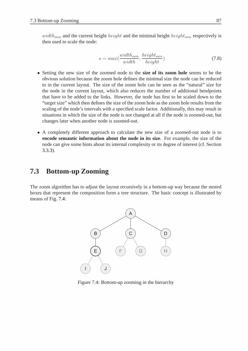
7.3 Bottom-up Zooming 87
widthmin and the current heightheight and the minimal heightheightmin respectively isthen used to scale the node:
s = max(widthmin
width,heightmin
height) (7.8)
• Setting the new size of the zoomed node to thesize of its zoom holeseems to be theobvious solution because the zoom hole defines the minimal size the node can be reducedto in the current layout. The size of the zoom hole can be seen as the “natural” size forthe node in the current layout, which also reduces the numberof additional bendpointsthat have to be added to the links. However, the node has first to be scaled down to the“target size” which then defines the size of the zoom hole as the zoom hole results from thescaling of the node’s intervals with a specified scale factor. Additionally, this may result insituations in which the size of the node is not changed at all if the node is zoomed-out, butchanges later when another node is zoomed-out.
• A completely different approach to calculate the new size ofa zoomed-out node is toencode semantic information about the node in its size. For example, the size of thenode can give some hints about its internal complexity or itsdegree of interest (cf. Section3.3.3).
7.3 Bottom-up Zooming
The zoom algorithm has to adjust the layout recursively in a bottom-up way because the nestedboxes that represent the composition form a tree structure.The basic concept is illustrated bymeans of Fig.7.4:
A
B C D
E GF H
JI
Figure 7.4: Bottom-up zooming in the hierarchy

88 Chapter 7. Zoom Algorithm
Lets assume that nodeE in Fig. 7.4is zoomed-out. NodesI andJ are removed from the currentdiagram as they are children of the now abstracted nodeE. The size of the zoomed-out nodeEshrinks which also reduces the size ofE’s parentB. NodeE has no sibling nodes so that nonodes insideB have to be moved. The zoom algorithm now has to adjust the positions ofB’ssiblingsC andD as the size ofB decreases. The reduced size ofB and the new position ofC andD in turn reduce the size of nodeA which is in this case the root node and therefore representsthe whole diagram. Thus, the zoom algorithm is applied recursively on all direct and indirectparents of the zoomed node as well as on the siblings of these ancestors. Note that nodesF , GandH can be ignored by the zoom algorithm because they are neitheran ancestor of the zoomednodeE nor a sibling of one of the ancestors. Thus, the zoom algorithm can only partially exploitthe partitioning of the decomposition structure because ofthe nested box notation: Changing thelayout on a lower level of the hierarchy entails additional changes on higher levels.

89
CHAPTER 8
Dynamically Generated Views
The zoom algorithm, as described so far, exploits the hierarchical structure of a model to generatedifferent views by showing only abstract representations of some model elements. However, theunderlying concepts of the zoom algorithm can also be used ina more general way in orderto adjust the layout if an individual node or a set of nodes is hidden in the current diagram.This filtering mechanism employs a secondary means to reducethe size and complexity of adiagram. Different views that display different facets of asystem (structure, data, behavior, userinteraction etc.) can be generated from a single integratedmodel by showing model elements ofcertain types only [Seybold et al., 2003]. Hence, a tool can be used to generate different viewsautomatically instead of forcing the modeler to create views himself by drawing a multitude ofdiagrams of different types, as required in UML for example (cf. Sections2.2.2and3.2). Thecombination of a fisheye zoom with such a view generation mechanism in a tool makes the useof comprehensive integrated modeling languages feasible.
The fisheye zoom which employs a vertical abstraction by suppressing all direct and indirectchildren of a node and the view generation mechanism which hides individual nodes or nodesof a certain type to abstract horizontally share the same underlying implementation. However,they can be used independently: Individual nodes or sets of nodes can be filtered regardless ofthe current zoom state of the diagram and zoom operations canbe applied on any dynamicallycreated view. Additionally, the generation of different views by filtering nodes of a specific typecan be used on flat (i.e., non-hierarchical) models too.

90 Chapter 8. Dynamically Generated Views
8.1 Node Filters
The specific kind of the views that are supported and which nodes should be shown in theseviews depends on the application the zoom algorithm is used in. However, the underlying idearemains the same: Generate views that show different parts of a model for a specific purpose(i.e., pragmatic criterion of a model [Ludewig, 2003]). Some exemplary views are the following:
• Views can be generated by showing or hiding all model elements that are instances of aspecific language construct. Different modeling facets (e.g., structure, data, behavior anduser interaction of a system) can then be shown by generatingdifferent views from a singleunderlying model [Seybold et al., 2003].
• All model elements that collaborate to fulfill a specific taskcan be shown in one view sothat the user can easily see those elements without being overwhelmed by a multitude ofelements that do not have anything to do with this task. Examples of such tasks are aspecific interaction between a set of objects or the behaviorthat is described by a (sub)setof states in a statechart [Harel, 1987].
• It is often desirable to see all nodes that are somehow related to the node that is currentlyinvestigated (cf. Section5.7). The filtering mechanism can be used to show all nodes thatare somehow (e.g., by a link) related to a selected node.
8.2 Filter Operation
The zoom algorithm described in the last chapter can withoutmodification be used for the fil-tering of nodes. The positions of the remaining nodes have tobe adjusted if a single node ora set of nodes is hidden. The zoom algorithm does exactly that, it adjusts the layout (i.e., theposition and size of the remaining nodes) if the size of a nodechanges. Thus, we can reuse thealgorithm by reducing the size of the node which should be hidden to a minimal size which inturn compacts the whole diagram. The size of the node is reduced to the smallest possible sizewhich iswidth(η′) = 1 andheight(η′) = 1 (it has to be> 0 in Equations7.1and7.2of Section7.2.1so that the scale factorssx andsy are> 0). The zoom algorithm is then used to recursivelyadjust the layout to this new (minimal) size of the node.
The example of Fig.8.1a) shows two nested interval structures: one for nodeA and one forA’s child B. NodesC, D andE are of a different type than nodesA andB (as indicatedby the different shapes) and should therefore be hidden in a subsequent view. The horizontalintervals ofA’s interval structure areX1 to X7 and its vertical intervalsY1 to Y7. The intervalstructure of nodeB consists of the horizontal intervalsX8 to X10 and the vertical intervalsY8
to Y10. We first consider the filtering of nodeE: The size ofE is reduced towidth(E ′) = 1andheight(E ′) = 1. The horizontal and vertical node intervals ofE, projx(E) = X9 and

8.2 Filter Operation 91
projy(E) = Y9 respectively, are scaled down toE’s new size. The length of the remaininghorizontal and vertical intervals (X8, X10 andY8, Y10 respectively) remains the same. Reducingthe lengths of the intervalsX9 andY9 reduces the size ofB’s interval structure which in turnreduces the size of nodeB.
X2
X3
X4
X5
X6
X7
X1
X9
X10
X8
A
B
X5
X6
X9
(a)
(b)
Y1
Y2
Y3
Y4
Y5
Y6
Y7
Y8
Y9
Y10
C
B
A
E
Y6
Y9
D
Figure 8.1: Filtering nodesC, D andE
Fig.8.1b) shows the situation after nodesC, D andE have been hidden. The lengths of intervalsX9 andY9 have been scaled to1 because the size of the node that is projected to these intervalshas been set to(1, 1) and no other node is projected to these two intervals. NodeE is too smallto be visible anymore but its position and size are indicatedby the dashed rectangle within nodeB in Fig. 8.1b). NodesC andD are hidden by using the same mechanism. However, the verticalintervalY3 cannot be scaled down completely while the height of nodeC shrinks because it is alsoa projection of nodeB (i.e.,Y3 ∈ projy(C) ∧ Y3 ∈ projy(B)) whose height is also reduced butnot by the same amount. The horizontal node intervals ofC, X5 andX6, can both be fully scaled

92 Chapter 8. Dynamically Generated Views
down so that the zoom hole of nodeC becomes the area marked with the second dashed rectanglein Fig.8.1b). The same holds for the horizontal node intervals ofD: The length of the horizontalintervalX3 cannot be fully scaled down because nodeB is also projected to this interval. Fullyscaling the horizontal intervalX4 removes the gap between nodesB andC as the length ofthe interval becomes1. Completely removing a gap between two nodes should be avoided asthe white space between nodes is an important part of the secondary notation (cf. Section2.5).Therefore, we introduce aminimal distancebetween two nodes and the constraint that the lengthof an interval that keeps two nodes apart must not fall below this threshold. The last horizontalnode intervalX5 of nodeD can be reduced to1 as it is only a projection ofC andD whichare both scaled down to(1, 1). While the minimal distance takes care that the zoom algorithmdoes not remove too much white space from the diagram, it may often be desirable to removemore white space than just the one that disappears with a hidden node. This can be achieved byadditionally scaling the gap intervals next to the node which is hidden. For example, the lengthof intervalX7 in Fig. 8.1can be reduced while nodeC is removed from the diagram in order toreduce the white space to the right of nodeB in Fig. 8.1b).
Hidden nodes can be shown again by setting the size of the nodeto its initial size and letting thezoom algorithm adjust the layout. Setting the size of nodesC, D andE in Fig. 8.1b) to theirinitial size and then using the zoom algorithm to adjust the position and size of the remainingnodes results again in the initial layout of Fig.8.1a). The size a node had before it was hiddenhas to be stored so that the node’s size can be restored once the node is shown again. Fortunately,this size (i.e., the size the node has if it is shown) is already stored in the node’s interval structure.Additionally, using the size of the interval structure makes it possible to set the size of the nodeto the correct value regardless of whether some of the children of the node are currently zoomed-out or hidden. Hiding nodeE in Fig. 8.1a) results in the new size of its parentB that is shownin Fig. 8.1b). If nodeB is then hidden and shown again in subsequent steps, the resulting layoutshould be that of Fig.8.1b) which is achieved by settingB’s size to the size of its intervalstructure. This works also correctly if the filtering of nodeE is undone beforeB is shown again:There is no immediate effect ifE is shown again, because its parentB is currently hidden, butshowingB in a subsequent step results again in the initial situation shown in Fig.8.1a).
Those fisheye techniques that are based on translation vectors like SHriMP or Berner’s approach(cf. Sections6.2and6.3respectively) cannot be used for such a node filtering mechanism becausethe filtering of a node is an extreme case of a zoom-out operation that is applied before the inversezoom-in operation: The new size is the minimal size the node can have and the node has to behidden (which is equivalent to the zoom-out) before it can beshown again (the equivalence ofthe zoom-in). The vector-based techniques cannot guarantee that the nodes in the adjusted layoutare still disjoint after a zoom or filtering operation in suchsituations.
Minimal Node size
Setting the size of the parent node to the size of its intervalstructure if one (or multiple) of itschildren are hidden can result in situations where the property of the minimal node size (cf. Sec-
8.2 Filter Operation 93
tion 5.10) does not hold anymore. For example, nodeB in Fig. 8.2a) should be hidden. Thesize ofB is reduced to the smallest possible size (i.e.,width(B′) = 1, height(B′) = 1) andthe zoom algorithm is used to adjust the layout toB’s new size. The fact that the width of nodeB is only marginal smaller than the width of the parent nodeA results in the situation that thewidth of A’s interval structure becomes smaller than the width of the predefined minimal nodesize. As a consequence, the filtering mechanism has to make sure that the width or height ofa node whose children are hidden does never fall below the threshold defined by the minimalsize of the node. Fig.8.2b) shows the situation where the width of the interval structure ofA issmaller than the width of nodeA. The only problem with this approach is that the user can inserta new node (or move an existing node) into the area inside nodeA that is no longer covered bythe interval structure (the hatched area in Fig.8.2b)). Thus, the zoom algorithm has to make surethat the interval structure is expanded accordingly if a node is inserted into or moved to this area,because the user must always be able to edit the model regardless of the current zoom or filterstate (cf. Section5.5).
A
B
A
(a)
(b)
Figure 8.2: Minimal size of nodeA if nodeB is hidden
Zooming-out versus Filtering
A zooming-out operation suppresses all children of a selected node while the filtering mechanismhides an individual node or a set of nodes. Thus, zooming-outcan be seen as a special instance ofthe filtering concept as it hides a set of nodes too (namely allchildren of a selected node). Usingthe filtering mechanism to hide all children of a node that is zoomed-out makes the calculationof the zoomed-out node size (cf. Section7.2.2) obsolete as the size of the node can just be setto the new size of the node’s interval structure (i.e., the size defined by the shape that remains ifall children of the node are filtered). This simplifies the whole concept because there is only oneoperation (i.e., filtering) required and the size of the zoomed-out node is calculated implicitly.However, this approach has two problems: First, the gap intervals between the children are notscaled while the nodes are hidden and may therefore avoid a substantial decrease of the node’ssize (which is desired to get a compact layout). The zoom algorithm has to scale the gap intervalsto avoid that the white space between the children bloats thesize of a zoomed-out node. The

94 Chapter 8. Dynamically Generated Views
second problem is that the size of the zoomed-in and zoom-outnode are tighter coupled so thatthey cannot be changed independently anymore. Changing thesize of the zoomed-out node doesalso change its zoomed-in size as the change is done on the interval structure.

95
CHAPTER 9
Editing Support
The nested box notation used to depict hierarchical relations lends itself to some kind of sophis-ticated tool support (like the fisheye zooming and view generation mechanism described in theprevious chapters) but the need for tool support, especially for the editing, is also significantlylarger than for ordinary (flat) graphs. A change in one part ofthe diagram is propagated all theway up in the hierarchy until the root node is reached. The user has to manually adjust the sizeof all direct and indirect parent nodes and possibly the location of their siblings to provide therequired space if a new node is inserted. Other editing operations such as removing or moving anode also result in a lot of tedious manual work for the user. Thus, a layout technique which au-tomatically expands or contracts parent nodes if a node is inserted or removed is highly valuable[Seybold et al., 2003] as it reduces the interaction overhead (cf. Section5.9) significantly. Ex-tending the fisheye and view generation technique to supportthe user while editing the diagrammoves it from a visualization technique to a more general “layout adjustment strategy” [Misueet al., 1995; Storey and Müller, 1995]. The extended zoom algorithm should not only permitediting operations (cf. Section5.5) but actively support them. A major advantage of the zoomalgorithm, presented in Chapter7, is that it can easily be used for automatic layout adaption ifthe diagram is edited by for example inserting or deleting a node.
User Control and Automation
While deciding on the amount of the layouting task that should be done automatically or manu-ally by the user, one inevitably faces a trade-off between the two properties of a small interactionoverhead (cf. Section5.9) and the freedom to use the secondary notation (cf. Section2.5). The
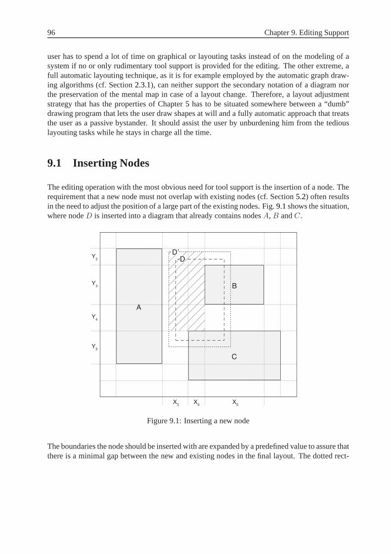
96 Chapter 9. Editing Support
user has to spend a lot of time on graphical or layouting tasksinstead of on the modeling of asystem if no or only rudimentary tool support is provided forthe editing. The other extreme, afull automatic layouting technique, as it is for example employed by the automatic graph draw-ing algorithms (cf. Section2.3.1), can neither support the secondary notation of a diagram northe preservation of the mental map in case of a layout change.Therefore, a layout adjustmentstrategy that has the properties of Chapter5 has to be situated somewhere between a “dumb”drawing program that lets the user draw shapes at will and a fully automatic approach that treatsthe user as a passive bystander. It should assist the user by unburdening him from the tediouslayouting tasks while he stays in charge all the time.
9.1 Inserting Nodes
The editing operation with the most obvious need for tool support is the insertion of a node. Therequirement that a new node must not overlap with existing nodes (cf. Section5.2) often resultsin the need to adjust the position of a large part of the existing nodes. Fig.9.1shows the situation,where nodeD is inserted into a diagram that already contains nodesA, B andC.
A
B
C
X3
X4
X5
D’Y
2
Y3
Y4
Y5
D
Figure 9.1: Inserting a new node
The boundaries the node should be inserted with are expandedby a predefined value to assure thatthere is a minimal gap between the new and existing nodes in the final layout. The dotted rect-

9.1 Inserting Nodes 97
angle marked withD′ in Fig. 9.1 shows thisexpanded nodewhile the dashed rectangle markedwith D represents the original boundaries of nodeD. The interval structure is then searched forthe space that the new node can maximally occupy without moving any sibling node away. Theresultingfree spaceis depicted by the hatched area in Fig.9.1. The node is then inserted with thesize of this free space by using the algorithm described in Section 7.1. The zoom algorithm is inthe next step used to increase the size of the node to its expanded size. The resulting situation forthe insertion of nodeD can be seen in Fig.9.2.
A
B
C
D’
X3
X4
X5
Y2
Y3
Y4
Y5
Figure 9.2: Situation after the expanded nodeD′ has been inserted
The space that is required to insert the expanded nodeD′ has been created by the zoom algorithmby moving the existing nodesB andC away (B towards the left andC towards the bottom). Thenode has been inserted with the size shown by the smaller dotted rectangle and then expandedto the size of the bigger dotted rectangle. The vertical interval Y2 of Fig. 9.1 has been splitinto the two intervalsY2 andY3 in Fig. 9.2 (see Section7.1 for a detailed explanation of howexactly the interval structure is updated if a new node is inserted). The zoom algorithm has thenscaled the length of the vertical and horizontal node intervals ofD′, namelyY3, Y4, Y5 andX4,X5 respectively to the length shown in Fig.9.2. Note that the scaling of the intervals has alsochanged the size of the zoom holes of nodesA,B andC (shown by the gray shaded areas) so thattheir boundaries are no longer congruent with the boundaries of the nodes they represent. Finally,the expanded node is removed from the interval structure (without scaling the intervals) and then

98 Chapter 9. Editing Support
inserted again with its original size. This results in a minimal gap between the new and existingnodes as the original size is smaller than the expanded size.The final situation for the insertionof nodeD into the diagram of Fig.9.1 is shown in Fig.9.3. The just presented technique canalso be used to provide additional white space in the diagramwithout actually inserting a node.
A
B
C
D
Figure 9.3: Final situation after nodeD has been inserted
9.1.1 Calculation of the Free Space
The maximal size a new node can be inserted with is calculatedbefore the zoom algorithmscales the intervals to provide the space that is required bythe new node. The impact on thecurrent layout (i.e., the amount of change) is minimized if the node is inserted with the size itcan maximally have in the current layout because the difference between this free space and theoriginal size becomes minimal. Additionally, the origin (i.e., the top left corner) of the calculatedfree space should be as close as possible to the origin of the boundaries the new node should beinserted with. The calculation of the free space can be realized by using the interval structureand a sequence of simple geometric and set operations. This algorithm to calculate the minimalspace is explained by means of Fig.9.4.
The basic idea is to first iterate over all horizontal intervals the new node lies in to find existing

9.1 Inserting Nodes 99
(a) (b)
(c) (d)
(e) (f)
(g) (h)
A
B
A
A A
A
A
A
A
B
B
B
B
B
B
B
X1
X2
X3
X4
X5
Figure 9.4: Calculation of the maximal available free space

100 Chapter 9. Editing Support
nodes that overlap with the new node. Second, the rectangleswhose origin lies as close aspossible to the origin of the new node and whose area covers asmuch of the area of the new nodeas possible without an overlap with an existing node are calculated. Finally, the biggest of theserectangles is selected. The detailed steps are the following:
1. Thefree spaceis set to the rectangle which represents the space that is required. Fig.9.4a)shows the situation where the maximal free space that is available for a new node in thediagram already containing nodesA andB should be calculated. Initially, the free space(represented by the hatched area) is set to the boundaries ofthe new node (the dottedrectangle).
2. The algorithm then iterates over all horizontal intervals covered by the boundaries of thenew node to check for overlaps with existing nodes. For the situation of Fig.9.4a) theseare the intervalsX1, X2 andX3. All nodes (or more precisely all zoom holes of the nodes)projected to the current interval in the iteration are checked for an overlap with the freespace. The first hit in the example of Fig.9.4a) is nodeA in intervalX2. The followingsteps are executed for each node for which such an overlap exists.
3. The overlapping existing node is subtracted from the freespace. NodeA is subtractedfrom the free space in Fig.9.4b), which results in the hatched polygon. The subtraction isa simple set operation:D = FS \A, whereD is the resulting set,FS the set representingthe free space andA the set representing nodeA. The free space is then set to the enclosingboundaries of the calculated area. If the resulting polygonis a rectangle, the solution hasbeen found. The following steps are executed only if the resulting areaD is not rectangular,as it is the case for Fig.9.4b).
4. The enclosing rectangle of the union between the free space and the bounds of the over-lapping node is calculated (the hatched area in Fig.9.4c)). This area is then horizontallyreduced to the part that covers the free space as well as the existing node. The resultingarea is shown by the hatched rectangle in Fig.9.4d).
5. The intersection between the resulting rectangle and thefree space is now subtracted fromthe polygon of step 3, which results in the hatched rectanglein Fig. 9.4e). The resultingrectangle is the first of the two candidate solutions.
6. Step 4 is now repeated in vertical direction: The enclosing rectangle of the union betweenthe free space and the bounds of the overlapping node is calculated and then verticallyreduced to the part that covers the free space as well as the existing node, as shown inFig. 9.4f).
7. The intersection between this resulting rectangle and the free space is now subtracted fromthe polygon of step 3, which results in the hatched rectanglein Fig. 9.4g). The resultingrectangle is the second of the two possible solutions.

9.2 Removing Nodes 101
8. The calculated free space is now set to the rectangle with the bigger area. For the example,this is the first solution shown in Fig.9.4e). The new node can then be inserted with thissize as shown in Fig.9.4h).
The next iteration of step 2 checks intervalX3 for an overlap between the free space and nodesA andB as they are both projected to this interval. However, no overlap is detected because thefree space has been reduced to the dotted rectangle of Fig.9.4h) during the first iteration.
9.1.2 Inserting Nodes Into a Partially Hidden Model
The view generation mechanism described in Chapter8 places some extra challenges on the al-gorithm that adjusts the layout in case of an editing operation because some of the existing nodesthat have to be moved may be hidden at the moment the operationtakes place. For example,the newly inserted node may overlap with an existing yet currently invisible node. However, ourzoom algorithm handles this situation without any modifications because the hidden node is stillin the interval structure (with a minimal size as described in Section8.2) and is moved away likeany other (visible) node.
9.2 Removing Nodes
The zoom algorithm should remove the empty space that becomes available if a node is removedfrom the diagram to fulfill the requirement of a compact layout (cf. Section5.1). The layoutadaption works the other way round as for the insertion of a new node: The size of the node thatshould be removed is first reduced to a minimal size to compactthe layout and the node is thenremoved from the interval structure. The zoom algorithm faces the same task of compacting thelayout as if a node is hidden to generate a specific view (cf. Section 8.2). The only differencebetween the two operations is that the node remains in the interval structure if it is hidden whileit is removed from the interval structure if the node is deleted.
The removal of a node is illustrated by means of Fig.9.5 where nodeB is removed from thediagram. The size of the node is reduced to the smallest possible size ofwidth(B) = 1 andheight(B) = 1. The zoom algorithm is then used to scale the affected intervals to adjust thelayout. The intervalsY3 andY4 are the vertical node intervals ofB (i.e., projy(B) = Y3, Y4)while X4 andX5 are its horizontal node intervals (i.e.,projx(B) = X4, X5). The length ofthese intervals is scaled when the size of nodeB is reduced as indicated by the two arrows. Thelength of intervalsY3 andX5 cannot be reduced because they are also projections of nodesA andC respectively which remain in the diagram (see Section7.2.2for a detailed discussion). Finally,the intervals that represent nodeB are removed from the interval structure (or more precisely,merged with their neighbored intervals as described in Section 7.1).

102 Chapter 9. Editing Support
C
A
X4
X5
B
X3
X6
Y2
Y3
Y4
Y5
Figure 9.5: Removing nodeB from the diagram
Fig. 9.6 shows the final situation after nodeB has been removed. The length of intervalsY4
andX4 have been reduced to1 to remove the resulting empty space from the diagram. Thismoves nodesA andB closer together and thereby reduces the overall size of the diagram. Thevertical intervalsY2 andY3 as well asY4 andY5 have been merged because these intervals are nolonger needed after nodeB has been removed. The same holds for the merging of the horizontalintervalsX3 andX4 as well asX5 andX6.
A
C
Figure 9.6: Final situation after nodeB has been removed
The layout can be further compacted during the removal of a node by not only scaling the nodeintervals but also their neighboring gap intervals (cf. Section 7.2.2). For example, consider againthe situation of Fig.9.5where not only the vertical node intervalsY3 andY4 but also the verticalgap intervalY5 is scaled when nodeB is removed. The scale factor for gap intervals has to be

9.3 Changing the Bounds of a Node 103
calculated separately because the one that is calculated for the node intervals reduces their lengthto the minimal length. The scale factor can for example be setto 0.5 so that the length of the gapintervals is halved. In the example of Fig.9.5only the gap intervalsY5 andX3 are additionallyscaled because intervalsY2 andX6 are also projections of nodesA andC and can therefore notbe scaled. NodesA andC are then closer together in the final layout of Fig.9.6.
9.3 Changing the Bounds of a Node
The boundaries of an existing node can, from a user’s point ofview, be changed by two differentediting operations: the node is moved (i.e., its coordinates change) or its size is changed (i.e., thewidth and/or height and possibly the location change). However, internally we do not have todistinguish between these two operations as they both require the same assistance from the zoomalgorithm. The operation of changing the bounds of a node canbe described as a combinationbetween the two previously discussed editing operations: The node is removed from its actuallocation with its current size and inserted at a new locationwith a new size. Therefore, the layoutadjustment that has to be done when the bounds of an existing node change can be realizedby combining the operations to remove and insert a node into one single operation. The majorproblem with this approach is that one single editing operation can result in multiple adjustmentsof the layout and therefore negatively influence the user’s mental map (cf. Section5.3) and thestability of the layout (cf. Section5.4). Additionally to this constantly changing layout, it canbecome difficult to calculate a new final layout if the second adjustment (after the reinsertion ofthe node) is based on a previous adjustment (the removal of the node).
9.4 Compacting Nodes
In our current tool implementation, we employ automatic layout adjustments only in situationswhere the moved or resized node overlaps with an existing node or lies partially outside theboundaries of its parent. We do not change the position or size of existing nodes if no overlapsoccur. This approach avoids situations in which a very smallchange of the position or size ofa node can have big impacts on the layout that cannot be understood by the user. As a conse-quence, we currently do not automatically compact the layout if the movement of a child resultsin additional white space even though this could easily be achieved. For example, if a node istoo close to the boundaries of its parent the size of the parent is increased to provide the requiredspace. If the node is then moved away from the parent’s border(i.e., to the inside of the parent),the size of the parent is not reduced automatically. Thus thewhite space at the border of theparent node grows. Automatically reducing the size of the parent node as soon as additionalwhite space becomes available can soon result in a multitudeof automatic layout adjustments sothat the whole layout starts to oscillate. Thus we do not support an automatic layout contractionduring the movement of child nodes (but of course during the removal of them). Instead, we

104 Chapter 9. Editing Support
provide an additional layout operation to compact a node (recursively) by scaling the length ofthe gap intervals down to a predefined value.

105
CHAPTER 10
Discussion of the Zoom Algorithm
The zoom algorithm and its extensions to generate differentviews from a single integrated modeland to actively support model editing presented in the last three chapters are now closely exam-ined in this chapter. The techniques are first discussed withrespect to the desired propertiesthat where presented in Chapter5. The second part of this chapter encompasses a more generalcriteria that has to be discussed for an algorithm, its runtime and space complexity.
10.1 Properties of the Zoom Algorithm
The properties that a zoom algorithm should have so that it can be used for visualizing and editinghierarchical models where presented in Chapter5. Each of these properties is now discussed indetail for our zoom algorithm.
Compact Layout
The zoom algorithm compacts the layout by scaling the lengthof the intervals the zoomed-outnode is projected to. Two independent scale factors for the horizontal and vertical intervals arecalculated from the current and new size of the node so that the amount the diagram shrinks inhorizontal and vertical direction can be different. How much an interval can be scaled downdepends also on the other nodes that are projected to it. Therefore, it is possible that the zoomalgorithm cannot adjust the layout of the model significantly if a node that “lies in the shadow”

106 Chapter 10. Discussion of the Zoom Algorithm
of another node is zoomed-out. NodeA is shadowed by nodeB if projx(A) ∩ projx(B) 6= ∅ orprojy(A) ∩ projy(B) 6= ∅.
For example, zooming-out nodesB andC in Fig.10.1a) results in a lot of free space between thetwo nodes in Fig.10.1b) because they are both shadowed by nodeA. NodesA andB are bothprojected to the vertical intervalY3 so thatprojy(A)∩ projy(B) = Y3 whileC andA are bothprojected toY5. While nodesB andC shrink because they are zoomed-out, intervalsY3 andY5
cannot be scaled down because the size of nodeA does not change. The height of the zoom holesof nodesB andC (the gray shaded area aroundB andC in Fig. 10.1b)) is bigger than the heightof the two nodes which results in the empty space between them. Unfortunately, there exists nogeneral solution for this problem as it is a manifestation ofthe trade-off between maintaining therelative position between nodesB andC on one side and the relative position between the twonodes and nodeA on the other side. This conflict cannot be resolved easily. However, nodesBandC are moved closer together as soon as nodeA shrinks too (e.g., when it is also zoomed-out)becauseY3 andY5 are then no longer blocked by a bigger node.
A
B
C
A
B...
C...
(a)(b)
Y3
Y5
D
E
Figure 10.1: NodesB andC are shadowed by nodeA
The shadowing of a node can result in situations where only the size of the zoomed node but notthe position of the siblings changes when a node is zoomed. Ifa node is completely shadowed byother nodes both in vertical and horizontal direction, noneof the horizontal and vertical intervalsit is projected to can be scaled so that the position of all sibling nodes and the size of the parentnode remains the same. NodeA is completely shadowed both in horizontal and vertical directionby nodesB andC if projx(A) ⊆ projx(B) ∧ projy(A) ⊆ projy(C).
Disjoint Nodes
The underlying interval structure of our zoom algorithm andthe concept of scaling interval sizesmake overlaps between nodes impossible. The horizontal andvertical intervals are stored andadjusted independently and the order within both of these sets is always maintained by the zoom

10.1 Properties of the Zoom Algorithm 107
algorithm. Fig.10.2 is used to illustrate that a zoom operation does never resultin overlapsbetween nodes which did not overlap before the operation took place. Let’s assume that thesize of nodeC is reduced because the node is zoomed-out. In principle, a zoom operation canproduce overlaps between the zoomed node and one (or multiple) of its siblings or among two (ormore) sibling nodes. An overlap between the zoomed node and one of its siblings is impossiblewith our zoom algorithm because only the intervals the zoomed node is projected to are scaled.For example, only the vertical node intervalY4 (and of course the horizontal intervalsX3, X4
andX5) but not the vertical gap intervalY3 that keeps nodesA andB apart from the zoomednodeC is scaled down. NodeC can never overlap with nodesA andB as long as the orderingof the vertical intervalsY2, Y3 andY4 is preserved. The same holds for any zoom-in operation.The ordering of the horizontal and vertical intervals is also the crucial point in avoiding overlapsbetween sibling nodes. The zoom algorithm has to prevent that nodesA andB in Fig. 10.2are moved too close together so that they overlap. An overlapbetween these two nodes is notpossible as long as the order of the horizontal intervalsX3, X4 andX5 is maintained. This isalways the case as the zoom algorithm scales intervalX4 (and even maintains a minimal lengthso that nodesA andB are kept away by a predefined distance) but never removes any of theintervals or changes their order.
A B
C
X3
X4
X5
Y2
Y3
Y4
Figure 10.2: NodesA, B andC are always disjoint after a zoom operation
The property that two nodesA andB do not overlap is true if the two following predicates hold:
projx(A) ∩ projx(B) 6= ∅ ⇒ projy(A) ∩ projy(B) = ∅ (10.1)
projy(A) ∩ projy(B) 6= ∅ ⇒ projx(A) ∩ projx(B) = ∅ (10.2)

108 Chapter 10. Discussion of the Zoom Algorithm
Predicate (10.1) states that the two nodes cannot share a vertical node interval (i.e., both areprojected to the same vertical interval) if they already share a horizontal interval. The secondpredicate (10.2) makes sure that two nodes cannot share a horizontal interval if they alreadyshare a vertical interval. For example, nodesA andB in Fig. 10.2share the vertical intervalY2
(i.e., projy(A) ∩ projy(B) = Y2) and cannot share a horizontal interval to fulfill predicate(10.2). It can easily be seen from Fig.10.2that they can only share a verticaland a horizontalinterval if they overlap at least partially. The zoom algorithm makes sure that (10.1) and (10.2)still hold after a zoom operation, if they did both hold initially (as they have to because the initiallayout would otherwise already contain overlaps), becauseit does neither change the order of theintervals nor the intervals the nodes are projected to (i.e., projx andprojy are still the same forall nodes after the zoom operation). Because the zoom algorithm is also used for the adaption ofthe layout after an editing operation, it can even make sure that a newly inserted or moved nodedoes not overlap with any existing node.
Preservation of the Mental Map
Theorthogonal orderingbetween nodes is preserved if the horizontal and vertical order of theircenter points is maintained (cf. Section5.3). Our zoom algorithm preserves the horizontal andvertical ordering of the intervals and therefore also the one of the boundaries of the zoom holes(as the boundaries of the zoom holes are defined by the boundaries of the intervals). However,that does not necessarily mean that the orthogonal orderingof the nodes themselves is also main-tained because their horizontal and vertical order dependson how they are positioned in theirzoom hole (if the zoom hole is bigger than the node).
Fig. 10.3shows an example. The vertical ordering of the nodes of Fig.10.3a) isB, C, A (thevertical position of the nodes’ centers is indicated by the dotted black linesYA, YB andYC).Fig. 10.3b) shows the situation after nodeA has been zoomed-out. The vertical ordering is nowB, A, C. The vertical position of the centers of nodesA andC is inverted because nodeA iscentered inside its zoom hole (the gray shaded area around nodeA in Fig. 10.3b)). In principle,it is possible to preserve the orthogonal ordering of the nodes’ centers by placing the nodes in adifferent way inside the zoom holes because the ordering of the vertical intervals is maintained.If the relative position of the center of nodeA inside its zoom hole is preserved from Fig.10.3a)to Fig. 10.3b), the vertical ordering of nodesA, B andC is also preserved (as nodeA is nowlocated at the bottom of its zoom hole).
However, other criteria can also have an influence on how the node should be placed inside itszoom hole. For example, it may be important that nodesA andB overlap vertically so that a linkbetween them can still be represented by a straight horizontal line after nodeA has been zoomed.The two nodes can no longer be connected by a straight horizontal line if nodeA is placed at thebottom of its zoom hole in Fig.10.3b) to preserve the relative position of its center in the zoomhole.Storey and Müller[1995] argue that thisstraightness of linksand the orthogonality of linksparallel to the X- and Y-axes is an important part of the mental map that should be preserved.

10.1 Properties of the Zoom Algorithm 109
A
B
C
B
CA...
(a)
(b)
YB
YC
YA
YB
YC
YA
Figure 10.3: The vertical orthogonal ordering between nodesA andD is not preserved
Maintaining theproximity relationsbetween nodes when one of them is zoomed-out seems tobe an easy task as the whole layout is compacted and the nodes are therefore moved closertogether anyway. However, two characteristics of the proximity relations make their preservationa challenge also in the case of a zoom-out operation: First, proximity relations do not only existbetween the zoomed node and its siblings but also among thesesiblings so that there is often atrade-off in deciding which of them should be maintained to what degree. And second, preservingthe proximity relations does not only mean keeping close nodes together but also maintaininga certain distance between nodes that where intentionally far apart in the initial layout. Forexample, consider the situation of Fig.10.4where nodeA is zoomed-out.
NodesB andC should still be close to nodeA after the zoom algorithm’s layout adjustments.However, it may be of importance too (as part of the secondarynotation) that there is a consid-erable distance between nodesC andD. Thus, the zoom algorithm has to find a compromiseso that all proximity relations in the diagram are preservedat least to some degree. The conceptof the zoom holes that can become bigger than the node they represent and the property that theordering of the intervals is maintained makes sure that the basic proximity relations between thezoom holes are always maintained. The proximity relations between the zoom hole of nodeA,represented by the gray shaded area around nodeA in Fig. 10.4b), and the zoom holes of theother nodes are still the same as they where in the initial situation of Fig.10.4a). The proximityrelations between the nodes themselves are not exactly the same anymore because they cannotall be maintained without destroying some other propertiesof the mental map. Maintaining the

110 Chapter 10. Discussion of the Zoom Algorithm
A
B C
D
B C
DA...
(a)
(b)
Figure 10.4: Maintain the proximity relations when nodeA is zoomed-out
horizontal distance between nodesA andD means that nodesD andC overlap horizontally inthe final layout which means that the ordering of the horizontal intervals is not the same any-more. Zooming-in nodeA of Fig. 10.4b) again preserves the proximity relations as it results inthe initial layout of Fig.10.4a). In contrast to the orthogonal ordering and proximity relations,the formaltopology preservationcriterion defined byMisue et al.[1995] cannot be investigatedwithout taking the links of the diagram into account (as the faces of a graph are defined by thelinks).
Layout Stability
The two most important properties of our zoom algorithm to guarantee the stability of the layoutregardless of the order of the zoom operations are the following: (i) the order and number ofintervals does not change during a zoom operation and (ii) the scaling is not done on the actuallength of an interval but on the real length that is stored forthe node whose size changes. Thestable order and number of the intervals guarantees that each zoom hole is still projected tothe same horizontal and vertical intervals after a zoom operation. The scaling of the real lengthinstead of the actual length makes sure that the length is setto the correct value even if it currentlydoes not have the length it should have after a preceding inverse zoom operation on the samenode. The zoom algorithm does the scaling for each node (or more precisely each zoom hole)that is projected to an interval separately and sets the interval’s actual length to the minimum ofthese values. Therefore, two zoom holes that are projected to the same interval cannot influenceeach other directly as the scaling is done on different values, namely their real length.
For example, consider the situation in Fig.10.5, where a sequence of zoom operations on nodesA andB results finally again in the initial layout. We consider onlythe horizontal intervals for

10.1 Properties of the Zoom Algorithm 111
this discussion because nodesA andB overlap in horizontal direction only. Zooming-out nodeA in Fig. 10.5a) results in the layout of Fig.10.5b). A’s zoom hole is projected to the horizontalintervalsX2 andX3 (i.e.,projx(A) = X2, X3). Thus, the zoom algorithm should scale thesetwo intervals when the size of nodeA is reduced. However, intervalX3 cannot be scaled becausethe zoom hole of nodeB is also projected to this interval. The zoom algorithm takescare of thisrestriction by not directly scaling the length of the interval but only the real length ofA’s zoomhole. This real length is stored separately for each interval the zoom hole is projected to.
(a)
(b)
(c)
(d)
A
B
A...
B
A...
B...
A
B...
X3
X4
X2
X3
X4
X2
X3
X4
X2
X3
X4
X2
Figure 10.5: Maintain the stability of the layout irrespective of the order of zoom operations
The width ofA is reduced by the factor0.5 so that the real length for the zoom hole of nodeA
is set to0.5 ∗ len(X2) and0.5 ∗ len(X3) for the intervalsX2 andX3. The actual length of theinterval is then set to the the maximal real length of all the zoom holes that are projected to the
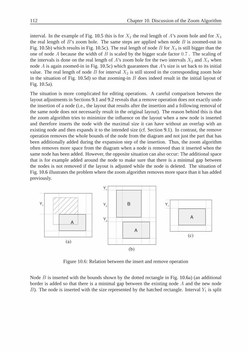
112 Chapter 10. Discussion of the Zoom Algorithm
interval. In the example of Fig.10.5this is forX2 the real length ofA’s zoom hole and forX3
the real length ofB’s zoom hole. The same steps are applied when nodeB is zoomed-out inFig. 10.5b) which results in Fig.10.5c). The real length of nodeB for X3 is still bigger than theone of nodeA because the width ofB is scaled by the bigger scale factor0.7 . The scaling ofthe intervals is done on the real length ofA’s zoom hole for the two intervalsX2 andX3 whennodeA is again zoomed-in in Fig.10.5c) which guarantees thatA’s size is set back to its initialvalue. The real length of nodeB for intervalX2 is still stored in the corresponding zoom holein the situation of Fig.10.5d) so that zooming-inB does indeed result in the initial layout ofFig. 10.5a).
The situation is more complicated for editing operations. Acareful comparison between thelayout adjustments in Sections9.1and9.2reveals that a remove operation does not exactly undothe insertion of a node (i.e., the layout that results after the insertion and a following removal ofthe same node does not necessarily result in the original layout). The reason behind this is thatthe zoom algorithm tries to minimize the influence on the layout when a new node is insertedand therefore inserts the node with the maximal size it can have without an overlap with anexisting node and then expands it to the intended size (cf. Section 9.1). In contrast, the removeoperation removes the whole bounds of the node from the diagram and not just the part that hasbeen additionally added during the expansion step of the insertion. Thus, the zoom algorithmoften removes more space from the diagram when a node is removed than it inserted when thesame node has been added. However, the opposite situation can also occur: The additional spacethat is for example added around the node to make sure that there is a minimal gap betweenthe nodes is not removed if the layout is adjusted while the node is deleted. The situation ofFig.10.6illustrates the problem where the zoom algorithm removes more space than it has addedpreviously.
A
A
B
A
(a)
(b)
(c)
Y1
Y1
Y1
Y2
Y3
Figure 10.6: Relation between the insert and remove operation
NodeB is inserted with the bounds shown by the dotted rectangle in Fig. 10.6a) (an additionalborder is added so that there is a minimal gap between the existing nodeA and the new nodeB). The node is inserted with the size represented by the hatched rectangle. IntervalY1 is split

10.1 Properties of the Zoom Algorithm 113
at the top boundary of the new nodeB and the resulting intervalY2 is scaled so that the wholenode fits in. Fig.10.6b) shows the resulting situation after nodeB has been inserted. The zoomalgorithm now reduces the length of intervalY2 of Fig. 10.6b) to 1 when nodeB is removedfrom the diagram. The length of the first vertical intervalY1 in the final layout of Fig.10.6c) isthen equal to the sum of the length of intervalsY1 andY3 in Fig. 10.6b) (plus1 from the scaledintervalY2). It can easily be seen that the final situation in Fig.10.6c) differs from the initialsituation of Fig.10.6a). The bounds a node has been inserted with (i.e., the boundsit had beforethe expansion phase of the zoom algorithm) have to be stored for a later removal if the removeoperation has to produce exactly the initial layout.
The main problem of editing operations that change the bounds of a node (cf. Section9.3) con-cerning the stability is that the zoom hole is reset to the current size of the node when a node isremoved and then reinserted. A zoom hole that is bigger than its node holds the information thatis required to preserve the stability of the layout (see Sections7.2.1and7.2.2for a detailed expla-nation). Because these informations are lost if a zoom hole is reset, the zoom algorithm can nolonger guarantee that the initial layout is restored if a zoomed-out node is moved or resized andthen zoomed-in again. That becomes a problem if small changes on the size or position of nodessuddenly result in significant layout changes after a subsequent zoom operation. It is usuallynot an issue for situations in which the user changes the layout himself significantly because hethen understands why the layout cannot be preserved in a subsequent zoom operation. Fig.10.7illustrates a situation where a slight movement of nodeB while it is zoomed-out compromisesthe stability of the layout. Fig.10.7a) shows the initial situation with nodeB zoomed in (itschildren are omitted since they are not relevant for the discussion). NodeB is then zoomed-out,as shown in Fig.10.7b) and moved slightly away from nodeA towards the bottom of the figurein Fig. 10.7c). Subsequently, zooming-in the moved nodeB results in the layout of Fig.10.7d)which differs from the initial layout of Fig.10.7a).
The reconstruction of the initial layout from the situationof Fig. 10.7b) relies on the fact that thezoom hole ofB (the gray shaded area aroundB) is bigger than the node itself. The informationthat the left boundary of nodeB is to the left of nodeA and its right boundary to the right ofnodeA is stored in the zoom hole. The size of the zoom hole is reset when the zoomed-out nodeB is moved in Fig.10.7c) because the node is first removed from the interval structure and theninserted again. The width of the new zoom hole of nodeB is now smaller than the width of thezoom hole of nodeA. The zoom algorithm tries to preserve this information by stretching thezoom hole of nodeA further in Fig.10.7d) so that it horizontally still covers the zoom hole ofnodeB. The size of the root node in the final layout is bigger than itssize in the initial layouteven though the geometric relations between nodesA andB are preserved (together with theslight downwards movement of nodeB). The same problem can occur if a new node is insertedinto the area that is occupied by the zoom hole which is biggerthan its node.

114 Chapter 10. Discussion of the Zoom Algorithm
A
B...
A
B...
A
B
A
B
(a)
(b)
(c)
(d)
Figure 10.7: Layout is no longer stable after an editing operation
Permit Editing Operations
The presented zoom algorithm does not only permit editing operations but actively supports themas described in Chapter9. However, this property comes not for free: Editing a diagram whilesome of its nodes are zoomed-out can make it impossible to guarantee the stability all the timeand preserve all properties of the mental map. The layout is not stable anymore if one or multiplezoom holes are reset during editing operations as describedin the last section.
Runtime
The evaluation whether our fisheye zooming techniques makesit possible to perform zoomingoperations with no remarkable delay has to be done by examining the runtime complexity of thealgorithm which is done in Section10.2.
10.1 Properties of the Zoom Algorithm 115
Multiple Focal Points
Each zoom operation is handled separately by our zoom algorithm so that the nodes can be inany zoom state (zoomed-in or zoomed-out) at any time. Havingmultiple nodes zoomed-in atthe same time shows the diagram with multiple focal points. The user can freely decide on thenumber and location of these focal points while the zoom algorithm guarantees the stability ofthe layout regardless of the number of focal points and the order they have been applied in.
Smooth Transitions
An animation of the transition between two layouts can be realized independently of the zoomalgorithm by linearly interpolating the nodes’ size and position between the initial and final value.Animating the layout changes does not only help in enhancingthe continuity for zoom operationsbut for any layout adjustment which is done by the zoom algorithm such as the generation ofdifferent views (cf. Chapter8) and the smart editing (cf. Chapter9).
Small Interaction Overhead
The interaction that is needed for a zoom operation is kept assimple as possible in our fisheyezooming approach: The user just has to click on a zoomed-out node to zoom into it while clickingon a zoomed-out node results in the abstracted view of the node. Clicking on a node “opens”or “closes” the node depending on its current state. The sizeof a node is always calculatedautomatically and is either defined by the space that is required by the node’s children or apredefined minimal size. A zoom operation does only change the size of the zoomed node andrecursively the size of its direct and indirect parents but never the size of one of its siblings.The sibling nodes are only moved to provide the required space or remove empty space fromthe diagram. This mode of interaction differs in its simplicity from other approaches such asSHriMP/Creole (cf. Section6.2) where the user first has to open a node by clicking on it andthen scale its size freely by holding the mouse button.
Minimal Node Size
A minimal node size is only needed for nodes whose children are all hidden because the node iseither zoomed-out or all its children are filtered out in a specific view. The size of the zoomednode’s siblings cannot fall below the minimal size as it is not changed at all. That is differentfrom other approaches such as SHriMP (cf. Section6.2) and the Continuous Zoom (cf. Section6.4) where the size of all nodes changes if one node is zoomed so that the diagram still fills thescreen completely after a zoom operation. Our zoom algorithm does not pose any restrictions onthe size a zoomed-out node should have so that it can be set to any predefined or calculated value(see Section7.2.2for a discussion of different ways to calculate the size of zoomed-out nodes).

116 Chapter 10. Discussion of the Zoom Algorithm
10.2 Algorithmic Complexity
Our fisheye zooming technique consists of two parts: the interval structure as the underlyingdata structure and the algorithms that work on this structure. The interval structure is constructedonly once and then adjusted if a zoom operation is applied. Therefore, we can examine thecomplexity of the interval structure construction and the zoom algorithm independently. Theinterval structure is constructed incrementally by inserting each node when it is added to thediagram as described in Section7.1. The algorithm to insert a node into the structure has linearcomplexity with respect to the number of intervals because it iterates (independently) over thehorizontal and vertical intervals. The same holds for the other operations that work on the intervalstructure (such as removing a node or adjusting its size) so that the number of intervals that astructure can maximally have defines the runtime complexityof the algorithms that work on it.An interval structure withn nodes can have at most2n+1 horizontal and2n+1 vertical intervalsas illustrated by Fig.10.8. Fig. 10.8a) shows the number of intervals for one node. There areat most three vertical and three horizontal intervals for a structure with one node. There may beless intervals if one boundary of the node overlaps with one boundary of the interval structure.Each additional node adds at most1 two vertical and two horizontal intervals. This is shown inFig. 10.8b) for a second node.
A A
B
(a) (b)
Figure 10.8: Number of intervals in the interval structure
For zoom operations, the complexity of adjusting the interval structure dominates the complexityof constructing the structures because the structures are only adjusted and not newly constructedif a node is zoomed. The runtime complexity of our zoom algorithm depends linearly on thenumber of intervals in the interval structure because the algorithm has to scale the node intervalsof the zoomed node to adjust the layout. Thus, the runtime andspace complexity are linearwith respect to the number of nodes. The linear runtime complexity guarantees that our zoomalgorithm can be used in an interactive environment. The space complexity is important becausesome informations (i.e., current and real length of the interval) about the structure have to bestored.
1The number of additional intervals is lower if the boundaries of the nodes are aligned.
Part III
Line Routing


119
CHAPTER 11
Lines in Graphical Models
The lines that are used to represent relationships between nodes in a diagram are often as impor-tant as the nodes themselves because the primary task of node-link diagrams is the visualizationof relations. The effort needed to recognize relations is largely determined by the drawing ofthe lines in the diagram. Crossings and overlaps between lines and nodes and among differentlines have a negative impact on the readability and understandability of a diagram. Such overlapsoccur frequently in the modeling domain where nodes can, in contrast to abstract graphs wherenodes take up little or no space, have a considerable size. However, manually arranging the linesso that such overlaps do not occur burdens a lot of additionalwork on the user who should bereleased from these tedious layouting tasks. Therefore, anautomatic line router that directs linearound nodes while trying to keep the lines as simple as possible is needed.
This chapter sets the stage for such an automatic line routerby first discussing the specific prob-lems of the routing task in hierarchical models (Section11.1) and in layouts that are constantlychanged and updated by zoom and/or editing operations (Section 11.2). These specific charac-teristics are taken up with a more general description of theline routing problem by discussing aset of requirements that a routing algorithm must meet (Section 11.3).
11.1 Lines in Hierarchical Models
The hierarchical relations in a diagram can either be depicted explicitly by links, as for examplethe composition and aggregation relations in UML’s class diagrams [OMG, 2005], or implicitly

120 Chapter 11. Lines in Graphical Models
by the nested box notation (cf. Section3.3.1). The nested box notation represents parent-childrelationships visually by the child being completely contained within the parent node. Thisreduces the number of links because some of the relations arerepresented implicitly. However,representing hierarchical decompositions by nested boxesalso entails some specific problemsconcerning the lines in the diagram.
11.1.1 Identifying Potential Obstacles
Lines in a hierarchical diagram often connect nodes locatedin different branches of the hierarchytree1. Therefore, it is not always obvious which nodes are potential obstacles for a line. Forexample, the bold nodes in Fig.11.1a) are the potential obstacles for the line connecting nodesF andJ . These nodes lie on different levels of the hierarchy. For example, nodesG andDare both potential obstacles even though nodeG is one hierarchical level below nodeD as caneasily be seen in the tree representation of Fig.11.1b). The potential obstacles of a line haveto be computed by traversing the hierarchy tree from nodep the line is completely contained in(which is nodeA in Fig. 11.1) to both the source and target node of the line. Thereby, all thenodes on each level which are not direct or indirect ancestorof either the source or target nodeare collected. Once the potential obstacles have been identified, the hierarchical line routingproblem becomes an instance of the usual “flat” line routing problem.
A
B C D E
F G H I J
(a)
(b)
G
B
H
C
D
I
E
A
J
F
Figure 11.1: NodesC, D, G andI are potential obstacles for the link betweenF andJ
1The hierarchy of the model can also be a forest (i.e., a set of trees with no single root node). In this case itcan easily be transformed into a tree by adding a “virtual” root node as parent for the existing root nodes of theindividual trees.

11.1 Lines in Hierarchical Models 121
11.1.2 Abstract Relationships
An additional problem that occurs only in hierarchically nested and never in flat models is thatlinks must reflect the hierarchical structure of the model: Arelationship between two nodes im-plies relationships on all hierarchical levels above thesenodes. Otherwise, the information thatthere exists a relationship between two nodes is lost if at least one of the direct or indirect par-ents of one of these nodes is zoomed-out. In ADORA these implied higher-level relationshipsare calledabstract relationships[Glinz, 2002; Glinz et al., 2002]. Moody [2006] uses the term“boundary relationships” andHarel [1987] calls them “stubbed entrance arrows” in his state-chart notation. For example, consider the situation of Fig.11.2which shows again the modelof Fig. 11.1a) but this time with nodeB zoomed-out. The relationship between nodesF andJcannot be shown by a link because nodeF is not visible when its parentB has been zoomed-out. The fact that there exists a relationship between nodeJ and one of the (currently invisible)children ofB is represented by an abstract relationship, drawn as a bold line, between nodesB andJ . The concept of abstract links guarantees that the model cannot become inconsistentconcerning the information flow between the objects represented as nodes [Glinz et al., 2002].However, for the line routing task it has the consequence that the lines have to be newly routedafter each zoom operation because existing lines can disappear and new lines emerge.
H
C
D
I
E
A
B...
J
Figure 11.2: Abstract relationship between nodesB andJ afterB has been zoomed-out
Both concepts, the calculation of the potential obstacles and abstract relationships, are onlyneeded if the links that can occur in a diagram are not restricted by the hierarchical relation-ship between their source and target node. No hierarchical restriction means that two nodes canbe connected by a link regardless of their position in the hierarchy. An explicit port concept, as itis for example employed in UML’s Composite Structure or Component Diagrams [OMG, 2005],constrains the connectivity so that links are only allowed between sibling nodes (i.e., nodes thatare on the same hierarchical level and have the same parent).This restriction reduces the com-plexity of the line routing task significantly because of thefollowing reasons: (i) the potential

122 Chapter 11. Lines in Graphical Models
obstacles do not have to be calculated because only the sibling nodes of the connected nodes arecandidates, (ii) the concept of abstract relationships is not necessary as the links never cross theboundaries of a node and (iii) the line routing algorithm canexploit the partitioning of the modelthrough the decomposition structure because a line never leaves the parent of the two nodes itconnects (which reduces the number of affected nodes).
11.2 Lines in a Dynamic Layout
The dynamic layout resulting from the zoom operations and the creation of different views in-tensifies the need for an automatic line router because the lines have to be adjusted to the newsituation after each layout change. It makes additional demands on the routing algorithm becausethe lines have to be routed in real-time in order to avoid thatthe runtime performance of the zoomalgorithm (cf. Section5.6) is adversely affected by the adjustment of the lines that has to be doneafter each zoom operation. As fisheye navigation requires the generation of a new diagram layoutin every navigation step, automatic and fast (i.e., real-time) line routing is essential and a manualadjustment of all lines is just not an option.
There are two possible ways of how to adjust a line if the layout changes due to a zoom operationor the switch to a different view: (i) Treat the bending points in the lines as nodes and let the zoomalgorithm handle them (as for example proposed byBartram et al.[1995] andBerner[2002]) or(ii) newly route the affected lines after each layout operation. The problem with the first solutionis that the layout changes that occur during a zoom operationcan have a big impact on a line eventough the overall layout is not changed dramatically. New bend points may become necessary toavoid that a line suddenly passes through a node and existingbend points can become obsoletebecause the line can now be routed in a more direct manner. Fig. 11.3shows an example wherethe line between nodesA andC can be routed directly without an additional bend after nodeB
has been zoomed out in Fig.11.3b) even though the overall shape of the diagram has not changedsignificantly.
In addition to the zoom algorithm, the layout can also be changed by the user directly when heedits the diagram. The tedious task of good line routing has be done automatically too when a di-agram is edited so that the modeler can concentrate on his primary goal of creating or modifyinga model. Diagrams are in the modeling domain usually createdmanually and incrementally bya human user and not automatically from an existing abstractrepresentation. Hence, we cannotcompute diagram layouts (including the lines) from scratchas done in graph drawing (cf. Section2.3.1) or the software visualizations in the reengineering field.Instead, we must be able to adapta given layout incrementally, preserving the secondary notation as far as possible. A dynamiclayout (i.e., zoom operations, view generation, interactive editing) results in some extra demandson the line routing algorithm but it is also the biggest advantage a tool has over a simple pa-per based modeling process. Thus, each algorithm that automates at least parts of this dynamiclayout creation is highly valuable.

11.3 Desired Properties of a Line Routing Algorithm 123
B
B...
(a)
(b)
A
C AC
Figure 11.3: Direct line between nodesA andC after nodeB has been zoomed-out
11.3 Desired Properties of a Line Routing Algorithm
The last section of this chapter briefly discusses the properties a line routing algorithm shouldhave so that it can be used for hierarchical dynamical modelsin a similar way as it was done forthe zoom algorithm in Chapter5. The lines in a graphical model or diagram have gained muchless attention in the literature and are often treated as a second rate citizen beside the nodes.That is a little bit surprising because the central task of node-link diagrams is to depict relations.Most of the work stems from the graph drawing field where the edges or links are often the mostimportant among the factors that govern automatic graph drawing algorithms (cf. Section2.3.1).
11.3.1 Bypass Nodes
The main rationale behind a line routing algorithm is to avoid that a line crosses freely throughnodes that lie between its source and target. The problems ofsuch overlaps between nodes andlines are that (i) the readability is reduced because the line may cross the label of the node, (ii) itbecomes harder to follow a line if it crosses the border of a node (which is in fact represented bya set of lines) and (iii) understanding the internals of a node in a hierarchical model is hardif lines that do not have anything to do with these internals are drawn (partially) inside thenode. Therefore, lines must not pass through nodes to avoid such node/link crossings. Overlapsbetween links and nodes become only a problem if the nodes take up a lot of space because ofa text label or nested child nodes in a hierarchical diagram.This is usually not the case in thegraph drawing field where the algorithms are designed for abstract graphs whose nodes take uplittle or no space [Misue et al., 1995].
124 Chapter 11. Lines in Graphical Models
11.3.2 Minimize the Length of a Link
Most automatic graph drawing algorithms (cf. Section2.3.1) try to avoid crossings between linksand nodes while placing connected nodes close together. Thus, minimizing the length becomesan integral part of the layout and is often not even mentionedas a specific requirement anymore.While layout algorithms can rearrange the nodes to reduce the length of the links this is not anoption for manually arranged diagrams. However, the links should still be as short as possible.This ensures that the user finds a link at the place he first looks for which is usually the areabetween the connected nodes.
11.3.3 Minimize Link Crossings
Since diagrams are a means of communication between different people with different back-grounds, it is crucial that the diagrams present information clearly. An empirical study by [Pur-chase et al., 2002] has revealed that minimizing the number of crossings between lines is themost important aesthetic that should be considered while trying to draw a diagram automatically(cf. Section2.4). Therefore, reducing the number of line crossings is one ofthe driving forcesbehind most graph drawing algorithms (cf. Section2.3.1). They try to place the nodes so thatcrossings between lines are avoided. A lot of these algorithms work only on planar graphs (i.e.,graphs that can be drawn without any edge crossings) so that agraph has to be “planarized” first(by for example deleting some of the edges). The situation isdifferent in the modeling domainwhere the position of the nodes is determined by the user, as an important part of the secondarynotation, and must not be changed by the line routing algorithm. Thus, the only option for theline routing algorithm is to find another path through the nodes that results in less crossings. Thedisadvantage of this procedure is the resulting trade-off between finding the shortest path andminimizing the number of line crossings that results because a line usually has to take a detourto avoid a crossing which in turn increases the length of the line.
11.3.4 Routing Styles
In contrast to other domains where lines or links are used (e.g., circuit design), diagram aestheticsplay an important role in the modeling domain.Battista et al.[1994] distinguish between threedifferent graphic standards or styles that have been proposed for the representation of graphs ina plane. The nodes are usually represented by graphical symbols such as circles or boxes andeach link is a simple open curve between the symbols associated with the start and end node.A drawing in which each link is represented by a polygonal chain is a polyline drawing. Twospecial cases of polyline drawings arestraight-linedrawings that map each link onto a straight-line segment andorthogonaldrawings that map each line onto a chain of horizontal and verticalsegments. The straight-line graphic standard is commonly adopted in the graph theory field whiletechnical diagrams such as Entity Relationship or UML diagrams are usually drawn according to

11.3 Desired Properties of a Line Routing Algorithm 125
the orthogonal graphic standard. Polyline drawings can also be modified to produce curved lines(i.e., splines).
The lines of a diagram have to be easy to follow and add clear meaning to the diagram.Wareet al.[2002] investigated the influence of different graph aesthetics on finding the shortest path ina set of graphs. Their primary focus was to show the importance of good continuity of the lines(i.e., keeping lines with multiple segments as straight as possible). The basic idea behind this isto exploit the Gestalt principle of continuity (which states that we are more likely to constructvisual entities out of visual elements that are smooth and continuous, rather than ones that containabrupt changes in direction) by using smooth and continuouslines as links [Ware, 2004, page191]. The results of their experiments showed that the continuity is, after the obvious length ofthe path itself, the most important factor in perceiving theshortest path. Therefore,Ware et al.[2002] state that it may be worth to accept an occasional crossing in a graph layout if it reducesthe “bendiness” of a line. Additionally, they argue that splines should be preferred to orthogonallines because their changes in direction are smoother and enhance continuity.
However, the semantic domain of the graph or diagram affectswhich aesthetic criteria need to beemphasized [Purchase et al., 2002] and it is impossible to state that some of the aesthetic criteriaare universally valid. The experiment byPurchase et al.[2002] revealed that non-orthogonaldrawings were preferred to orthogonal drawings because of the increased number of bends in theorthogonal lines. But orthogonality was then in fact preferred in the semantic domain of UMLclass and collaboration diagrams. One of the reasons for this may be that in most areas that usediagrams for visualizing information a preferred style or consensus about how a line should looklike has emerged (e.g., orthogonal lines in circuit diagrams or UML diagrams). People are usedto that style and become confused if this convention is violated. Additionally, the results indicatethat the overall layout has an impact on how a line should looklike. Diagrams that consists ofmostly rectangular figures seem to be candidates for orthogonal lines while straight lines seemto be more suited for rooted trees such as family trees or organization charts.
It is possible to take advantage of the fact that none of the proposed line routing styles is objec-tively superior to any of the others. Different line routingstyles can be combined in one diagramto route different kinds of links with different styles. This technique simplifies the distinctionof different kinds or types of relationships but makes the line routing task harder because therouting algorithm has to support different routing styles.
11.3.5 Mental Map and Secondary Notation of a Line
Which characteristics of a line are part of its secondary notation and influence the user’s men-tal map is much less examined than in the case of the nodes’ characteristics (cf. Section5.3).North [1996] argues that the preservation of the mental map concerning the nodes is much morecrucial than the preservation of the lines’ mental map. The rationale behind this is that nodesare landmarks that a user can learn and return to in a diagram,while lines are usually traced on

126 Chapter 11. Lines in Graphical Models
the fly to discover relations or connections2. If lines are indeed secondary in the preservation ofthe mental map, it becomes advantageous to adjust the lines aggressively (e.g., by newly routingthem after each layout adjustment) to improve the layout, while moving nodes more conserva-tively. Improving the layout means in this context fulfilling some of the general aesthetics suchas minimizing the number of line crossings or bends in a line.
However, Fig.11.4shows that the line routing may have an important effect on the overall lookand thus on the mental map of a node-link diagram: Diagrams a)and b) look different eventhough the underlying structure (i.e., the underlying graph) and even the location and size of thenodes are the same. The differences result solely from varying the position of the lines’ start andend point on the boundary of their start and end node. Therefore, completely ignoring the lineswhile considering the mental map of a diagram may result in a significant disorientation of theuser. A discussion of metrics to formalize and measure the mental map of a line can be found inSection5.3.
(a) (b)
Figure 11.4: Line routing and the mental map [Bridgeman and Tamassia, 2000]
Besides their influence on the formation and preservation ofthe mental map, some character-istics of a line may, additionally to the aesthetic criteria, have an influence on the readabilityand understandability of a diagram. The direction of the information flow has emerged as animportant aesthetic feature during the experiments ofPurchase et al.[2002]. The direction ofthe information flow is foremost defined by the position of thenodes that are connected. Theposition of a node is either defined by the user or the zoom algorithm and must not be changedduring the line routing. But the direction of information flow can be emphasized by selecting theposition of the start and end point on the boundaries of the start and end node accordingly. Theexample of Fig.11.5shows a repeated sequence of stepsA, B andC with an information flowfrom top to bottom. This direction convention is preserved for the line connecting nodesC andA in Fig. 11.5a) as the line leaves nodeC at the bottom and enters nodeA at the top even toughC is located belowA. As a result, the repeating pattern can be recognized a lot easier than in thesyntactically equivalent layout of Fig.11.5b).
2This is also the reason why it is much more common to hide linksand not nodes to reduce the complexity of adiagram.

11.3 Desired Properties of a Line Routing Algorithm 127
A
B
C
A
B
C
(a) (b)
Figure 11.5: Secondary notation employed in a line
Thus, the routing algorithm has to give off some control to the user so that he can at least partiallyinfluence the final shape of the line to encode additional information in its secondary notation.This can for example be achieved by letting the user determine the start and end point of the line.The routing algorithm must then preserve this secondary notation as far as possible if the line is(re)routed after a layout operation. However, the preservation of the secondary notation or mentalmap and the aesthetic criteria such as a minimal length of theline or a minimal number of linecrossings are competitive so that the optimality of one often prevents the optimality of others. Forexample, the line between nodesC andA in Fig. 11.5a) is longer than strictly necessary becausethe secondary notation is used to show the direction of the information flow consistently.
11.3.6 Runtime
The runtime complexity of the routing algorithm is an important issue because the lines haveto be routed in real time whenever the modeler changes the layout of a model by navigating,creating a view or editing (cf. Section11.2). Thus, the line routing algorithm must be able toroute a large fraction of all lines in a diagram without a remarkable delay. The concrete numberof lines that have to be rerouted depends on how many nodes arechanged by the layout operationand how the lines are embedded into the hierarchy.


129
CHAPTER 12
Existing Line Routing Approaches
The problem of routing a line around a set of obstacles occursin many different domains. Sincethe detailed requirements and constraints for the routing of a line vary slightly from domain todomain, different techniques have evolved rather separately and isolated from each other. Thefollowing sections give a short overview over different techniques from various domains anddiscuss their applicability to graphical models with respect to the desired properties presented inSection11.3. The first section covers the routing of lines or edges by automatic graph drawingalgorithms. Section12.2 describes the use of a visibility graph for the routing that plays animportant role in computational geometry. Approaches to route wires in the circuit design fieldare discussed in Section12.3. Finally, Section12.4presents a technique that has been developedespecially for incrementally created models of software systems.
12.1 Lines as Part of the Automatic Graph Drawing
In the automatic graph drawing field the routing of lines or edges is an integral part of the auto-matic graph drawing algorithm (cf. Section2.3.1). One of the main goals of such an algorithm isin fact to avoid line crossings. The routing of the lines is foremost optimized by placing the nodesin a manner that reduces crossings between lines. Two characteristics of graphical models renderthe application of this integrated layouting and routing approach impossible. First, the layout isusually done manually and incrementally by the user in orderto exploit the secondary notation(cf. Section2.5) and must not be changed dramatically in case of a small change to preserve theuser’s mental map. And second, most of the automatic graph drawing algorithms were originally

130 Chapter 12. Existing Line Routing Approaches
designed for abstract graphs were nodes take up very little or no space [Misue et al., 1995]. Incontrast, the graphical representations of nodes in graphical models of software systems take upa considerable part of space, especially if they employ the nested set notation (cf. Section3.3.1).
12.2 Routing on the Visibility Graph
The “geometric shortest path problem” in computational geometry has many applications inrobotics, geographic information systems and diagram drawing (see e.g. [de Berg et al., 2000]for an overview). Probably the best known approach constructs a visibility graph and computesthe shortest path on this graph according to Dijkstra’s algorithm [Dijkstra, 1959]. Fig. 12.1showsan example of a simple visibility graph used to route a line that connects pointsS andT alongthe obstacles represented by the gray rectangles. The vertices of the visibility graph (shown bythe little circles in Fig.12.1) are the corners of the obstacles together with the start andend pointof the path. There exists an edge between two verticesv andw if the two vertices can “see”each other (i.e., the straight line segmentvw does not intersect the interior of any obstacle). Theshortest path (or more precisely one of the shortest paths since it needs not be unique) can thenbe found by assigning the Euclidean length of an edge as its weight and then using Dijkstra’sshortest path algorithm. The black vertices and edges in Fig. 12.1constitute the shortest pathbetween pointsS andT .
S
T
Figure 12.1: Visibility graph
Relying on a visibility graph for the routing of lines in a graphical model yields two problems.First, the avoidance of line crossings cannot be integrateddirectly into the shortest path calcu-lation on the visibility graph. This is due to the fact that the visibility graph does not containany informations about existing connections between nodes(i.e., it represents only the relationsbetween the corners of nodes in the original layout). Thus, crossings between lines have to bedetected and resolved in an (expensive) second step after the basic routing. And second, the rout-ing is restricted to straight line drawings since the edges in the visibility graph are direct straight

12.3 Grid-Based Routing 131
lines. Orthogonal lines that are common in technical drawings or models cannot be deduced in astraightforward manner from such a visibility graph.
12.3 Grid-Based Routing
The circuit design domain has evolved independently from the automatic graph drawing fieldeven though the circuits constitute with their electronic elements as nodes and the wires as edgesa graph. This is due to mainly two reasons: First, the layout of circuits has to satisfy techni-cal (e.g., maximal lengths of the wires or the prohibition ofwire crossings) instead of aestheticcriteria. Additionally, the prohibition of line crossingsimplies that the lines cannot be routedindependently from each other. Instead, there has to be a specific order in which lines are routedsince an already routed line becomes a potential obstacle for subsequent lines. And second, incontrast to the integrated view in the graph drawing field, the layouting of the circuit (i.e., theposition of the elements) and the routing of the wires are treated as two separate steps. Further-more, the number of nodes and links is, especially in the fieldof highly integrated circuits (VLSI:Very Large Scale Integration), with several millions very high.
The wires in electric and electronic circuits are almost exclusively routed orthogonal. Only someanalog circuits employ an angular routing style. Because wire crossings are not allowed, wiresare usually not only routed on one plane but on several stacked layers. Therefore, the routingtakes no longer place in a 2D space but in a 3D space. However, for the following discussion werestrict ourselves to two dimensions since the presented concepts can easily be extended to threedimensions. Almost all wire routing techniques operate on auniform grid structure. Becausethe wires have to be routed on this structure around existingelectronic elements that representobstacles like in a maze, this concept is often called “maze routing”.
12.3.1 Lee’s Algorithm
The first and perhaps best known algorithm for grid-based routing in circuit designs is Lee’salgorithm [Lee, 1961] which is an application of Dijkstra’s breadth-first shortest path searchalgorithm [Dijkstra, 1959] to a uniform grid. Lee’s algorithm is based on the expansionof adiamond-shaped wave from the source point that continues until the target point is reached.Fig. 12.2shows an example to find a path connecting grid cellsS andT . The gray shaded cellsrepresent obstacles that cannot be crossed by a wire or line.The first and second step of the waveexpansion are show in Fig.12.2a) and b), while c) shows the situation after the eighth iterationwith the wave approaching the end cellT . The shortest path can then be found in a secondstep by going back from the target point to the source point while selecting the neighbored gridcell with the lowest value. This is illustrated by the hatched cells in Fig.12.2d). The algorithmalways finds a solution if one exists, and ensures an optimal solution. The major drawback ofthis approach is that its space and runtime complexity isO(mn) for a grid withm∗n cells which

132 Chapter 12. Existing Line Routing Approaches
makes it unsuitable for an interactive use. Several techniques have been proposed to reduce thespace and runtime complexity of the algorithm. For example,the approach ofSoukup[1978]combines the breadth-first with a depth-first search by looking always into the direction of thetarget without changing the direction. Only after hitting an obstacle, the algorithm falls back to abreadth-first search. However, this approach sometimes results in suboptimal solutions and canstill not reduce the large number of cells which constitute the uniform grid structure.
1
1S
T
2
1
1
2
2
2
S
T
5 4 3
2
4
3
5 6
4 5
7
6
2 1
1
2
2
3
3 4
4 5
5
6
6
7
3 2
4 3
3
4
7
8
8
5 4 5
6 7 8
7
8
8
7
8
8S
T
5 4 3
2
4
3
5 6
4 5
7
6
2 1 2 3 4 5 6
3 2
4 3
3
4
7
8
5 4 5
6 7 8 9
9
10
7
8
8
9
9 10
10 11
11
7
8
8
9
9
10
10
11
2
12
12
(a) (b)
(c) (d)
1 2 3 4 5 6
7
8
9
10
11
S
T
Figure 12.2: Lee’s algorithm

12.4 Routing in Incremental Layouts 133
12.4 Routing in Incremental Layouts
The concept ofMiriyala et al.[1993] explicitly addresses the problem of routing lines in modelsof software systems that are incrementally constructed by the user by adding nodes and links oneafter the other. Their approach produces orthogonal lines (since that is the routing style that ismost commonly used in graphical models of technical systems) and tries to minimize the numberof crossings among lines, the number of bends in lines and their overall length. The concept isvery similar to our own algorithm1 presented in the next chapter. The two main differences arethat we use a different underlying data structure (tiles instead of segments) and that we separatethe path (or channel) finding from the actual routing of the line. These two characteristics makeit possible to employ additional routing styles while the concept of Miriyala et al. is restricted toorthogonal lines.
The data structure that is used by Miriyala et al. is the so called rectangulation. It represents eachnode as a rectangle and each link as a sequence of horizontal and vertical segments (thus therestriction to orthogonal lines). The reason for this subdivision into rectangular regions is thatbends or crossings can only result from a movement from one region to another. The rectangula-tion is constructed by drawing a so called virtual vertical segment from every critical point (i.e.,corner point of a node or bend point in a line) that extends up to the next object that obstructs thepath. Fig.12.3shows an example:
Figure 12.3: Rectangulation
The gray rectangles and lines in Fig.12.3 represent the original nodes and links. The dashedlines illustrate “edge segments” (i.e., vertical segmentsof the existing links), the continuous
1We developed our algorithm independently since we were not aware of the concept ofMiriyala et al.[1993] atthat time.

134 Chapter 12. Existing Line Routing Approaches
black lines “vertex segments” (i.e., vertical bounds of thenodes) and the dotted lines “virtualsegments” which are added to construct the rectangulation.Dijkstra’s shortest path algorithm[Dijkstra, 1959] is then used as a heuristic to find line routings on this structure similar to ourown approach as presented in Sections13.2and13.3.

135
CHAPTER 13
Tile Maze Router
The major problem of Lee’s algorithm presented in the last chapter is the large number of cellsin the grid structure. The resulting runtime and space complexity can be reduced by applyingthe basic idea of the algorithm to a sparse structure insteadof a uniform grid. This “cornerstitching data structure” and some of the basic operations that can be applied to it are presentedin Section13.1. Our line routing approach is divided into two completely decoupled steps: Thefirst step, described in detail in Section13.2, computes one or multiple paths through which theshortest path has to pass. The second step which computes theline itself (i.e., the bend points ina polyline) is shown in Section13.3. Extensions of the basic algorithm are presented in Sections13.4, 13.5and13.6. The chapter finishes with a discussion of our algorithm in Section 13.7. Apreliminary version of the algorithm has already been presented in [Reinhard, 2004; Reinhardet al., 2006].
13.1 Data Structure
Instead of a uniform grid we use the corner stitching structure [Ousterhout, 1984] as the un-derlying data structure for the line routing. The corner stitching structure has originally beendeveloped as an efficient storage mechanism for VLSI layout systems and has two importantfeatures:
• All space, whether occupied by a node or empty, is explicitlyrepresented in the structure.This explicit representation of the empty space makes it possible to provide fast geometri-

136 Chapter 13. Tile Maze Router
cal algorithms to locate the space that is available for the routing.
• The space is divided into rectangular areas that are stitched together at their corners like apatchwork quilt. These corner stitches allow easy modifications of the structure and leadto efficient implementations of a variety of geometric operations.
The corner stitching structure for the four nodes of Fig.13.1a) is represented by the dashed lines.The space is divided into a mosaic with rectangular tiles of two types: space tilesand nodetiles. Tiles must be rectangles with sides parallel to the X and Y axes. The only constraint isthat nodes must not overlap. This has to be guaranteed by other techniques such as the onesdescribed in Chapters7 and9. The space tiles are organized as maximal horizontal strips: nospace tile ever has another space tile immediately to its right or left. However, there can beanother space tile directly above or below a space tile. Thisorganization ensures that there is oneand only one decomposition of the empty space into space tiles for each arrangement of nodetiles. The maximal horizontal strip representation is crucial for the space and time complexityof the geometric operations. Fig.13.1b) shows in detail how the tiles are linked by a set ofpointers, called corner stitches, at their corners.Ousterhout[1984] uses only four pointers (twoat the bottom-left and two and the top-right corner) insteadof eight. We use the additional fourpointers for our extension to minimize line crossings (cf. Section13.4).
A
B
C
D
(a)
(b)
lt
tl
bl
lb rb
br
tr
rt
Figure 13.1: Corner stitching structure
The advantage of a corner stitching structure with maximal horizontal strips over a uniform gridstructure is its linear space complexity: while the number of cells in a uniform grid is determinedby the size and the resolution of the grid, the maximum numberof space tiles in the corner stitch-ing structure only depends on the number of nodes. In a diagram with n nodes, there will never

13.1 Data Structure 137
be more than3n+1 space tiles (see [Ousterhout, 1984] for a proof). Additionally, all operationson the corner stitching structure depend only on informations of their local neighborhood so thatthe size of the overall diagram has no negative influence on their runtime. However, this clearupper bound can only be achieved by a higher space complexity(i.e., we face an instance ofthe runtime-space trade-off). The corner stitching structure requires at least three times morememory than a simple linked list since it requires empty space to be represented and uses moreneighbor pointers. Fortunately, the space complexity is not a big problem for diagrams as thenumber of nodes is usually at most several hundred and reaches never the millions of nodes thatare no exception in the VLSI domain.
The question that remains is why we have to use an additional data structure for the line routinginstead of just reusing the interval structure that is already used by the zoom algorithm (cf. Sec-tion 7.1). The problem is that the horizontal and vertical intervalsare independent in the intervalstructure because we want to scale them independently. The intervals do not represent an areaof the layout but are in fact projections from the two-dimensional Euclidean space to a one-dimensional space. For the line routing algorithm we need a structure that divides the plane in aset of areas or tiles because we want to use the basic algorithm of Lee[1961] which works on atwo-dimensional representation of the space.
Finding the Tile at a Given Location
One of the most common geometric operations in a diagram is tofind the node at a given(x, y)location. For example, this operation can be conducted eachtime the mouse pointer is movedto find the node it currently points to. The simplest but also least efficient solution for thisproblem is to sequentially iterate over a list containing all nodes in the diagram. This approachhas linear runtime with respect to the number of nodes in the diagram. The corner stitchingstructure permits a much more sophisticated algorithm to find for each pointp, represented by itscoordinates(x, y), the tile the point lies in. The algorithm can be used to search for both, nodeand space tiles. It iterates in horizontal and vertical direction over the tiles, starting from anygiven tile in the structure:
1. The algorithm follows the corner stitches pointing to thetop and bottom neighbor of a tile(lt andlb in Fig. 13.1b)), until a tile is reached whose vertical range contains the verticalposition of the desired pointp.
2. From this tile it moves to the right or left, by following the tr andtl stitches, until a tile isfound whose horizontal range contains the horizontal position of the desired pointp.
3. This horizontal movement can result in a vertical misalignment (i.e., the tile that was foundduring the horizontal search in step 2 does not contain the vertical position of the desiredpoint) so that steps 1 and 2 may have to be repeated several times to locate the tile con-tainingp. Whether a point is located in a tile can easily be found out bycomparing theboundaries of the tile and the position of the point.
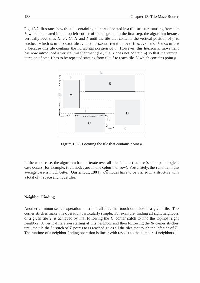
138 Chapter 13. Tile Maze Router
Fig. 13.2illustrates how the tile containing pointp is located in a tile structure starting from tileE which is located in the top left corner of the diagram. In the first step, the algorithm iteratesvertically over tilesE, F , G, H andI until the tile that contains the vertical position ofp isreached, which is in this case tileI. The horizontal iteration over tilesI, C andJ ends in tileJ because this tile contains the horizontal position ofp. However, this horizontal movementhas now introduced a vertical misalignment (i.e., tileJ does not containp) so that the verticaliteration of step 1 has to be repeated starting from tileJ to reach tileK which contains pointp.
J
K
E
A
B
C
D
F
H
I
p
G
Figure 13.2: Locating the tile that contains pointp
In the worst case, the algorithm has to iterate over all tilesin the structure (such a pathologicalcase occurs, for example, if all nodes are in one column or row). Fortunately, the runtime in theaverage case is much better [Ousterhout, 1984]:
√n nodes have to be visited in a structure with
a total ofn space and node tiles.
Neighbor Finding
Another common search operation is to find all tiles that touch one side of a given tile. Thecorner stitches make this operation particularly simple. For example, finding all right neighborsof a given tileT is achieved by first following thetr corner stitch to find the topmost rightneighbor. A vertical iteration starting at this neighbor and then following thelb corner stitchesuntil the tile thebr stitch ofT points to is reached gives all the tiles that touch the left side ofT .The runtime of a neighbor finding operation is linear with respect to the number of neighbors.

13.1 Data Structure 139
Construction of the Corner Stitching Structure
At the beginning, the corner stitching structure consists of one single space tile that occupies thewhole layout. Node tiles are then incrementally inserted for each node in the diagram. Becausewe use the structure only for the line routing and not any other layouting task, we construct thestructure after the layout (i.e., position and size of the nodes) has been established. Therefore,we can assume a correct layout and do not have to check whetherthe node that is inserted intothe structure overlaps with an existing node (even though such a test can easily be performedwith the corner stitching structure). The algorithm to insert a tile into an existing structure isillustrated by means of Fig.13.3.
B
B
B
B
A A
AA
(a) (b)
(c) (d)
P1
P2
Figure 13.3: Inserting a tile into the corner stitching structure
1. The algorithm to find a tile at a given location is used to search for the space tile thatcontains the top-left border of the node to be inserted (P1 in Fig. 13.3a)). The organizationof the corner stitching structure guarantees that the wholetop boundary of the node lies inone single tile.

140 Chapter 13. Tile Maze Router
2. The found space tile is split along the line defined by the top boundary of the node to beinserted as shown in Fig.13.3b). This implies that the corner stitches of the involved tilesand its neighbors are updated.
3. The algorithm to locate a tile at a give point is now again used to find the space tile thatcontains the bottom-left corner of the node that should be inserted (P2 in Fig. 13.3a)).
4. This bottom space tile is, in analogy to step 2, split and the corner stitches are adjusted sothat they point again to the correct neighbors.
5. The algorithm now iterates vertically over the tiles starting from the top tile of the new nodeuntil the bottom tile is reached. During this iteration eachtile has to be split vertically intwo new tiles: one to the left and one to the right of the new node. Space tiles are wheneverpossible vertically merged into one tile. Thereby, the corner stitches of the involved tilesand their neighbors are adjusted.
The runtime of the algorithm depends on the effort that is required for the splitting and mergingof the tiles. This effort is determined by the number of tilesthat have to be visited (i.e., theneighborhood of the new node). The merging and splitting canin the average case be donein constant runtime as long as the new tile has about the same size as the tiles around it (see[Ousterhout, 1984] for a detailed discussion).
On-the-fly Construction
Because the construction of the corner stitching structurerequires some effort and even toughthe runtime becomes only a problem in really large diagrams,the question arises of how to storethe structure after its initial construction. In principleit would be possible to construct a cornerstitching structure for each node in the hierarchy (by inserting the children of the node one afterthe other into the structure) and then store it. That is in fact the same strategy that was used forthe interval structure that is used for the fisheye zoom (cf. Section7.1). However, the problemwith this approach is that the corner stitching structures are not bound to a specific node butrather to a specific line because the potential obstacles fora line (i.e., the nodes that have to beinserted into the structure) are defined by the hierarchicalposition of the line’s start and end node(cf. Section11.1). Storing a structure for each line instead of node is possible but requires that itis updated after each layout change. Because the removal andreinsertion or movement of a tilecan become quite complex and a new structure can be constructed with a justifiable effort, it iseasiest to construct a new structure each time a line is routed.

13.2 Channel Finding 141
13.2 Channel Finding
The first step of our routing algorithm computes the path(s) of space tiles through which the linehas to pass by applying the fundamental wave expansion idea of Lee’s algorithm to the cornerstitching structure instead of a uniform grid structure. During the expansion phase the algorithmcomputes a distance value for the space tiles of the structure. Due to the non-uniform tile size,it is not possible to use the distance from the source point toeach of the tiles as distance value,because there may be multiple different values for one tile.Therefore, we use a combination ofthe source distance and the distance to the target point which are both measured in the Manhattandistance1. Furthermore, for each tile the algorithm computes the point P inside the tile where thedistances are actually measured. For the actual search, an ordered data structure (e.g., a heap ora priority queue) denoted asΩ is used. The algorithm consists of the following steps:
1. The corner stitching structure is constructed and tileTstart that contains the source points
and tileTend that contains the target pointt are identified.
2. PointP for Tstart is set to the source points, the source distance ofTstart to 0 and thedistance ofTstart to the Manhattan distance betweenP and the target pointt. Tstart is theninserted intoΩ.
3. As long asΩ contains tiles: TileT with the lowest distance value is removed fromΩ. Ifthis tile isTend, a path has been found. Otherwise, pointPnext (i.e., the point insideTnext
closest to the pointP of the current tileT ) is calculated for each neighboring space tileTnext. For each of these neighboring tiles two distance values arecalculated: Thesourcedistanceσ is calculated by adding the Manhattan distance between point P and pointPnext
to the source distance ofT . Thedistanceδ is calculated by adding the Manhattan distancebetweenPnext and the target pointt to σ. Equations13.1and13.2show the calculationof the source distanceσ and the distanceδ for the tileTnext relative to the tileT , whereasλ(P1, P2) denotes the Manhattan distance between the pointsP1 andP2:
σ(Tnext) = σ(T ) + λ(P, Pnext) (13.1)
δ(Tnext) = σ(Tnext) + λ(Pnext, t) (13.2)
The calculated distance value forTnext is compared to the previously calculated value forTnext (if there is one). If it is lower, the distanceδ and source distanceσ values ofTnext areupdated. TileTnext is then inserted intoΩ.
4. The sequence(s) of space tiles that constitute the shortest path can be found, in analogyto Lee’s and Dijkstra’s algorithm, by moving back fromTend to Tstart while repeatedly
1The Manhattan distance, also known as the L1-distance, between two pointsP andQ is defined as the sum ofthe lengths of the projections of the line segments onto the coordinate axes:λ(P,Q) = |xP − xQ|+ |yP − yQ|

142 Chapter 13. Tile Maze Router
selecting a neighbored tile that has the same distance valueδ. If multiple neighbors havethe same value, there exist multiple solutions and the current tile is a branch.
Fig. 13.4illustrates the proceeding of the routing algorithm by means of a simple example. Asan initial simplification, we assume that the start and end point of the line have already beenprojected from their nodes to one of the space tiles around the node by some means (cf. Section13.5). Thus, the start points lies now in the space tileT1 below nodeA and the end pointt inspace tileT6 above nodeD.
A B
C D
δ(T1)=271
A B
C D
δ(T2)
=415
δ(T3)
=273
δ(T4)=271
A B
C D
δ(T7)
=375
δ(T5)
=413
A B
C D
δ(T2)
=415
δ(T1)=271
δ(T3)
=273
δ(T4)=271
δ(T7)
=375
δ(T5)
=413
δ(T6)=271 δ(T
6)=271
(a) (b)
(c) (d)
s=P1 s
s
t t
t t
P2
P4
P3
P7
P6P
5
Figure 13.4: Finding a path of space tiles froms to t
PointP1 of tile T1 is set to the start points, the source distanceσ(T1) to 0 (because the distancebetweens andP1 is zero as they are at the same position) and the distanceδ(T1) to the Manhattandistance between pointsP andt which is271. T1 is then inserted into the ordered data structure

13.3 Bend Points Calculation 143
Ω and immediately removed again in the next step because it is the first and only tile that iscurrently inΩ. The algorithm now calculates the pointPnext for each of theT1’s neighbors,T2,T3 andT4, as shown by the dotted black lines in Fig.13.4b). The resulting points areP2 forT2, P3 for T3 andP4 for T4. The next step is to calculate for each of these neighboring tiles thesource distanceσ and the distanceδ. For tileT4, for example, the source distance is calculatedaccording to formula (13.1) by adding the Manhattan distance betweenP1 andP4 to the sourcedistanceσ(T1) of the current tile which results inσ(T4) = 32. The distanceδ(T4) is computedaccording to formula (13.2) by adding the distance betweenP4 and the target pointt to the justcalculated source distanceσ(T4). The Manhattan distanceλ(P4, t) is 239 so that the distancefor tile T4 is equal to271. T4 has the same distance value as tileT1 because the increase in thesource distance is compensated by the decrease of the distance to the target whenP moves awayfrom the source point closer to the target point. That is not the case for tiles that lie on a paththat goes into the “wrong direction” (i.e., further away from the target point instead of closerto it) like for example tileT2 for which both the source distance and the distance to the targetincrease. The combined distance value and the fact that the tiles are taken from an ordered datastructureΩ results in a directed search instead of Lee’s undirected search which propagates in alldirections. The ordered data structure makes sure that the algorithm does automatically look foran alternative path as soon as it is stuck with the most promising one. Fig.13.4c) shows the nextiteration through step 3 of the algorithm:T3 has been removed fromΩ because it is the tile withthe lowest distance and the distance values for its neighbors T5, T6 andT7 are calculated. Thepath has been found as soon asT6 is processed in the next iteration because it contains the endpoint t. The gray shaded rectangles which represent in Fig.13.4the tiles for which the distancevalues are currently calculated show how the wave expands from s towardst. Fig. 13.4d) showshow the sequence of the space tilesT6, T4 andT1 that constitute the shortest path can finally befound by repeatedly selecting a neighbored tile with the same distance value as the current one.
13.3 Bend Points Calculation
The algorithm for finding the space tiles the shortest path has to pass through is completelydecoupled from the algorithm that does the actual routing (i.e., computes the coordinates fordrawing the line). Hence, different algorithms that produce different styles of lines can be im-plemented on top of the algorithm described in the last Section.
13.3.1 Orthogonal Lines
As an example, we have implemented an orthogonal line routerthat produces rectilinear poly-lines. The algorithm starts with the path returned by the path finding algorithm and iterates overall tiles in the path by repeatedly following the reference to the next tile. The line is routed insidea space tile with respect to the direction the line enters andleaves the tile. In the following, thefour possible directions are named by the points of the compassnorth, south, eastandwest. We
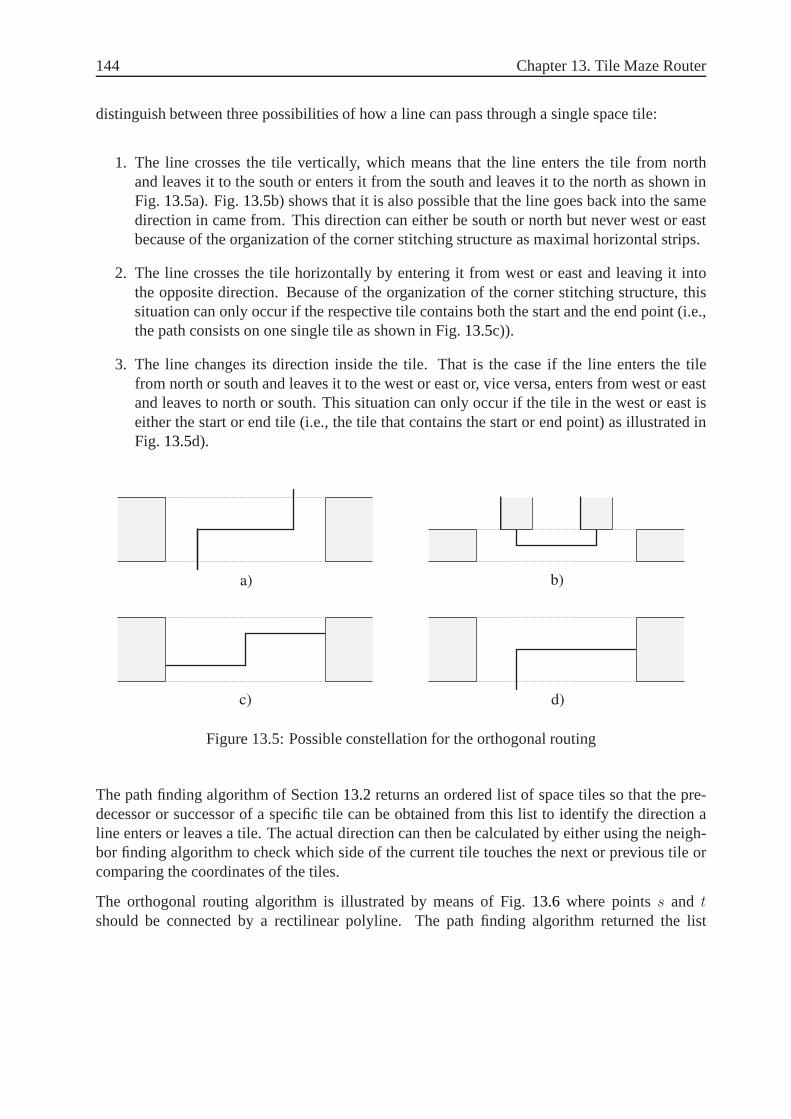
144 Chapter 13. Tile Maze Router
distinguish between three possibilities of how a line can pass through a single space tile:
1. The line crosses the tile vertically, which means that theline enters the tile from northand leaves it to the south or enters it from the south and leaves it to the north as shown inFig. 13.5a). Fig.13.5b) shows that it is also possible that the line goes back into the samedirection in came from. This direction can either be south ornorth but never west or eastbecause of the organization of the corner stitching structure as maximal horizontal strips.
2. The line crosses the tile horizontally by entering it fromwest or east and leaving it intothe opposite direction. Because of the organization of the corner stitching structure, thissituation can only occur if the respective tile contains both the start and the end point (i.e.,the path consists on one single tile as shown in Fig.13.5c)).
3. The line changes its direction inside the tile. That is thecase if the line enters the tilefrom north or south and leaves it to the west or east or, vice versa, enters from west or eastand leaves to north or south. This situation can only occur ifthe tile in the west or east iseither the start or end tile (i.e., the tile that contains thestart or end point) as illustrated inFig. 13.5d).
a) b)
c) d)
Figure 13.5: Possible constellation for the orthogonal routing
The path finding algorithm of Section13.2returns an ordered list of space tiles so that the pre-decessor or successor of a specific tile can be obtained from this list to identify the direction aline enters or leaves a tile. The actual direction can then becalculated by either using the neigh-bor finding algorithm to check which side of the current tile touches the next or previous tile orcomparing the coordinates of the tiles.
The orthogonal routing algorithm is illustrated by means ofFig. 13.6 where pointss and t
should be connected by a rectilinear polyline. The path finding algorithm returned the list

13.3 Bend Points Calculation 145
〈T1, T2, T3, T4, T5〉 marked by the gray shaded tiles in Fig.13.6a). The basic idea of the orthog-onal routing algorithm is to adjust the horizontal interval(or “window” [Miriyala et al., 1993])through which a vertical segment has to pass while iteratingover the space tiles. The number ofbends in the line is minimized by routing the line without changing its direction as long as pos-sible. We assume that the start points is fixed so that the initial horizontal interval is reduced tothe horizontal position of the start point (i.e., left boundary l and right boundaryr of the intervalare set to the x coordinate ofs) as shown by the dotted black line in Fig.13.6a). The next tile inthe path isT2 so that the horizontal segment through whichT2 can be reached fromT1 has to bedetermined.
This interval, represented by the dotted black lines in Fig.13.6b), does not overlap with theprevious interval of Fig.13.6a) so that two new bend points have to be added to the line. Bothnew bend point are vertically centered inT1 and the second one is horizontally centered withinthe horizontal interval. The horizontal interval remains the same for the next tileT3 in Fig.13.6c)because its width is only reduced but never increased (i.e.,the left boundaryl of the interval isonly moved to the right and its right boundaryr only to the left). Its width has to be reduced forthe next tileT4 by moving its right boundary to the left. The last bend point in the line is movedso that it is still horizontally centered within the interval. This is can be done without problemsbecause the new and the previous interval do overlap. The next tile T5 does not demand anyaction as the horizontal interval lies completely within the horizontal bounds of the tile. Finally,the interval is reduced to the horizontal position of the endpoint t because the position of thispoint is fixed (as part of the secondary notation). The intervals of Fig.13.6e) and Fig.13.6f) donot overlap so that two additional bend points are required.
Because of the organization of the corner stitching structure as maximal horizontal strips, itsuffices to calculate the horizontal interval. A vertical interval is not needed because it is alwaysdefined by the height of the tile. Fig.13.6shows that the vertical crossing of a line through atile is by far the most common situation (in fact the line crosses all tiles in Fig.13.6vertically)because the other possibilities of how a line can pass through a tile (i.e., situations b), c) andd) in Fig. 13.5) are all special cases. Only the vertical crossing requiresthe calculation andadjustment of the interval because the information that is needed to insert a new bend point cannot be influenced by the previous or next tile in the other situations.
One drawback of the organization of the corner stitching structure as maximal horizontal stripsis that it can, together with the concept of inserting additional bend points as late as possible,result in suboptimal lines. The problem occurs if the line passes through multiple tiles verticallyand changes its direction in the last of these tiles. It is then only vertically centered within thelast tile even though it should be vertically centered within the area that is defined by multipletiles (in order to better exploit the available space and maximize the distance to the node it passesaround). Fortunately, the line can easily be adjusted in a second step because the whole emptyspace is explicitly represented in the corner stitching structure.

146 Chapter 13. Tile Maze Router
(a) (b)
s
T1
T2
T3
T4
T5
t
T2
(c) (d)
T3
t
T4
(e) (f)
T5
t
l=r=sx l r
l r l r
l r l=r=tx
Figure 13.6: Calculate the bending points for an orthogonalline
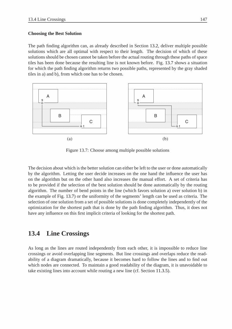
13.4 Line Crossings 147
Choosing the Best Solution
The path finding algorithm can, as already described in Section 13.2, deliver multiple possiblesolutions which are all optimal with respect to their length. The decision of which of thesesolutions should be chosen cannot be taken before the actualrouting through these paths of spacetiles has been done because the resulting line is not known before. Fig.13.7shows a situationfor which the path finding algorithm returns two possible paths, represented by the gray shadedtiles in a) and b), from which one has to be chosen.
A
B
C
s
t
A
B
C
s
t
(a) (b)
Figure 13.7: Choose among multiple possible solutions
The decision about which is the better solution can either beleft to the user or done automaticallyby the algorithm. Letting the user decide increases on the one hand the influence the user hason the algorithm but on the other hand also increases the manual effort. A set of criteria hasto be provided if the selection of the best solution should bedone automatically by the routingalgorithm. The number of bend points in the line (which favors solution a) over solution b) inthe example of Fig.13.7) or the uniformity of the segments’ length can be used as criteria. Theselection of one solution from a set of possible solutions isdone completely independently of theoptimization for the shortest path that is done by the path finding algorithm. Thus, it does nothave any influence on this first implicit criteria of looking for the shortest path.
13.4 Line Crossings
As long as the lines are routed independently from each other, it is impossible to reduce linecrossings or avoid overlapping line segments. But line crossings and overlaps reduce the read-ability of a diagram dramatically, because it becomes hard to follow the lines and to find outwhich nodes are connected. To maintain a good readability ofthe diagram, it is unavoidable totake existing lines into account while routing a new line (cf. Section11.3.5).
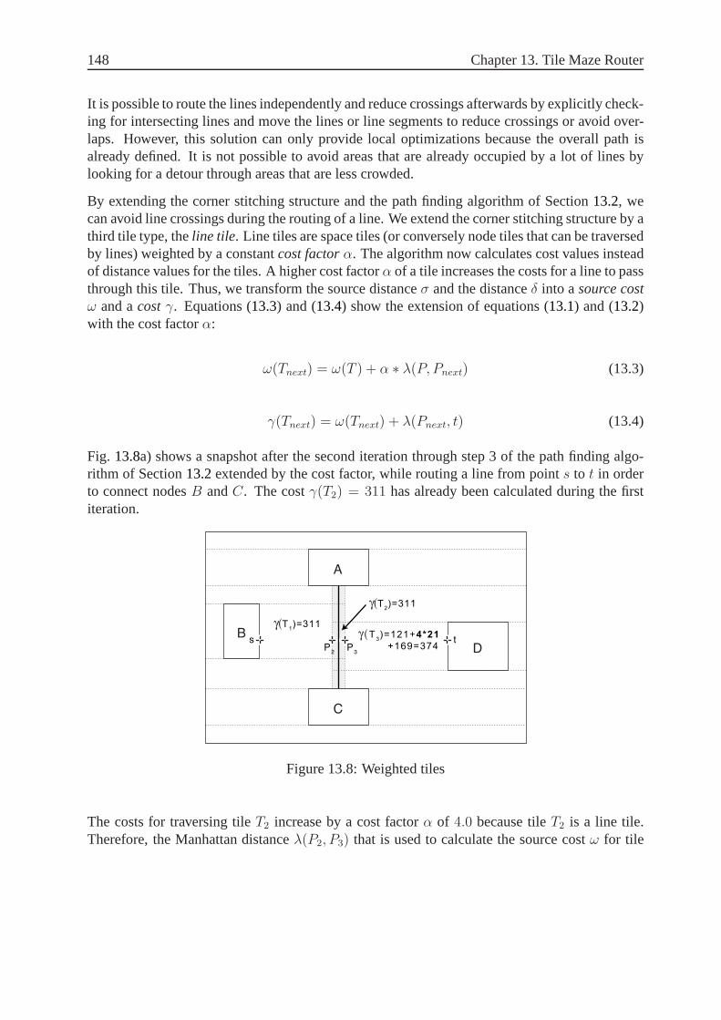
148 Chapter 13. Tile Maze Router
It is possible to route the lines independently and reduce crossings afterwards by explicitly check-ing for intersecting lines and move the lines or line segments to reduce crossings or avoid over-laps. However, this solution can only provide local optimizations because the overall path isalready defined. It is not possible to avoid areas that are already occupied by a lot of lines bylooking for a detour through areas that are less crowded.
By extending the corner stitching structure and the path finding algorithm of Section13.2, wecan avoid line crossings during the routing of a line. We extend the corner stitching structure by athird tile type, theline tile. Line tiles are space tiles (or conversely node tiles that can be traversedby lines) weighted by a constantcost factorα. The algorithm now calculates cost values insteadof distance values for the tiles. A higher cost factorα of a tile increases the costs for a line to passthrough this tile. Thus, we transform the source distanceσ and the distanceδ into asource costω and acostγ. Equations (13.3) and (13.4) show the extension of equations (13.1) and (13.2)with the cost factorα:
ω(Tnext) = ω(T ) + α ∗ λ(P, Pnext) (13.3)
γ(Tnext) = ω(Tnext) + λ(Pnext, t) (13.4)
Fig. 13.8a) shows a snapshot after the second iteration through step 3of the path finding algo-rithm of Section13.2extended by the cost factor, while routing a line from points to t in orderto connect nodesB andC. The costγ(T2) = 311 has already been calculated during the firstiteration.
γ(T1)=311
γ(T2)=311
γ(T3)=121+4*21
+169=374P3
BDP
2
ts
C
A
Figure 13.8: Weighted tiles
The costs for traversing tileT2 increase by a cost factorα of 4.0 because tileT2 is a line tile.Therefore, the Manhattan distanceλ(P2, P3) that is used to calculate the source costω for tile

13.5 Calculation of the Start and End Point 149
T3 is multiplied by the cost factor of line tileT2. Adding the source costsω to the Manhattandistance to the target results according to Equation (13.4) in a cost valueγ of 374 for tile T3. Thecost factorα can now be used to express the detour of a line the user is willing to accept to avoida crossing with another line. Increasingα in Fig. 13.8a) suddenly results in a line that is routedalong the top boundary of nodeA because this path becomes “cheaper” than the path that crossesthe existing line. The idea of tiles weighted by a cost factoris not restricted to line tiles. It maymore generally be used to influence the routing of a line by indicating preferred areas or parts ofthe diagram that should be avoided.2
Step 4 of the path finding algorithm (cf. Section13.2) has to be extended so that neighbors withthe sameor a lowercost value are selected during the retracing. The cost valuebecomes lower,if a line is crossed during the retrace. The drawback of this approach is that the number of pathsthat are found during the retracing increases because (i) the number of tiles increases with theadditional line tiles and (ii) a path can go through any of these line tiles which results in a largernumber of potential paths. To reduce the number of potentialpaths, we store the origins of atile (i.e., the neighbored tile(s) from which the cost valueof the actual tile has been calculated)during the expansion phase. We can then just follow these references during the retrace. A tile isadded as origin to one of its neighbored tiles if the cost value that is calculated for this neighboris equal to the current cost of the neighbor. If the calculated cost value is lower than the currentcost value of the neighbored tile, all existing origins are removed.
This collecting of the origins during the expansion phase demands an additional invariant on thecorner stitching structure in order to make the algorithm work in all situations as expected: Aline tile can never have multiple tiles as left or right neighbors. If a line tile touches two or moretiles on the left or right side, it has to be split accordingly. This is the reason why there are fiveline tiles in Fig.13.8a) instead of only one that covers the whole existing line. This invariantmakes sure that the space tile that lie on the other side of a line are “visible” through the lineso that each tile on the other side of a line can be reached directly without traveling a long wayinside the costly line tile. Additionally, the orthogonal routing algorithm of Section13.3.1has tobe generalized to work correctly on this extended corner stitching structure because (line) tilesare now frequently crossed horizontally (i.e., the situation of Fig.13.5c) does now also occurwhen a line crosses an existing line). In addition to the horizontal interval, the algorithm has tomaintain a vertical interval in order to route a line correctly in horizontal direction.
13.5 Calculation of the Start and End Point
So far we have assumed that the start and end point of a line areat fixed positions that lie onthe boundaries of the nodes (or more precisely in the space tiles that touch the boundary of thenode). That is the case for tools that offer a set of “connectors” or “magnets” on the boundary ofa node that can be used as the start and end point of a line. Thisconcept leaves some control over
2We use a cost factorα for each tile in our current implementation which is set to1.0 for ordinary space tiles.

150 Chapter 13. Tile Maze Router
how the line should look to the user while it constrains the possibilities by offering only a smallnumber of connectors. The decision on the position of the start and end point has to deal witha trade off between the amount of control left to the user and the part done automatically by therouting algorithm. On the one hand, the effort that is required to route a line should be reducedas much as possible which demands for a maximal degree of automation. The required effortcan easily become unbearable in the case of a dynamic layout where the position and size of thenodes change while existing lines disappear and new lines emerge (cf. Section11.2). But on theother hand, the position of the start and/or end point can be an important part of the secondarynotation that is only known to the user. For example, the direction of the information seemsto have a big influence on the understandability of a diagram (cf. Section11.3.5) so that it canbecome important that a line ends at the top boundary of a nodeeven though the shortest pathends at one of the other boundaries.
The concept of weighted tiles that was introduced to reduce the number of line crossings canalso be used to calculate the start and end point of a line by projecting any point inside the nodethat has been selected by the user to the node’s boundary. Thebasic idea is to start the lineinside the start node (and no longer inside a neighbored space tile) and add a high cost factorto this start node so that the line tries to leave the node as fast as possible. Thus, the user caninfluence the location a line starts and ends at by setting thisclick pointclose to one of the node’sboundaries. The routing algorithm then tries to find a compromise between starting the line asclose as possible to the user’s click point and the overall length and shape of the line.
γ(T1)=539
γ(T3)=413
γ(T2)
=511
γ(TA)=340
γ(T4)=365
γ(T5)=365 γ(T
B)=381
P4
P5
s
t
P2
P3
P1
PB5
PB4
Figure 13.9: Calculating the position of the start and end point
Fig. 13.9shows an example where the pointss andt which lie now inside the start and end nodehave to be connected. The expansion phase of the path finding algorithm remains the same, but itnow starts inside the start node and not in a neighbored spacetile anymore. The costsγ(TA) areset to the Manhattan distance betweens andt because the source distanceω(TA) is initially 0.The first iteration calculates now the costs for the neighbors of tileTA. The Manhattan distancefrom s to pointsP1, P2, P3 andP4 is, according to Equation (13.3), multiplied by a cost factor of

13.5 Calculation of the Start and End Point 151
α = 1.8. The resulting source costsω are then added to the distance to the target which results inthe costsγ(T1) = 539, γ(T2) = 511, γ(T3) = 413 andγ(T4) = 365 (the cost value is truncatedto an integer during the calculation). TileT4 has the lowest cost value amongA’s neighborsbecause it can be reached by traveling the shortest distanceinside the costly node tileTA. Asa consequence, the user can influence the selection of the space tile in which the line starts byselecting an appropriate click point inside the node. The path finding algorithm proceeds withtile T4 as this is now the tile with the lowest cost value. In the next step, the end tileTB can bereached fromT4 so that a solution has been found.
The decision on whether the current tile is now added as origin to the end tile is a little bit morecomplicated. The algorithm has to ensure that the position of the end point inside the end nodehas also an influence on the final line. The cost value for the end tile TB is calculated by addingthe Manhattan distance betweenP4 and the pointPB4 (i.e., the point insideT4 that is closest tothe pointt) to the Manhattan distance between this pointPB4 andt multiplied by the cost factorof TB. We can ignore the distance to the target which is0 because the target has been reached sothat the cost forTB is calculated according toγ(TB) = ω(T4) + λ(P4, PB4) + α ∗ λ(PB4, t) orwith the concrete numbers of Fig.13.9, γ(TB) = 56 + 288 + 1.8 ∗ 21 = 381 (again truncated toan integer). The same calculation is done for the path that reachesTB throughT5 which results inγ(TB) = 105 + 189 + 1.8 ∗ 71 = 421. This cost value is bigger than the one that was calculatedfrom T4 so thatT5 is not added as an origin toTB. Therefore, the final path isPA, P4, PB. Aline through this path contains more bend points than a path that would go thoughPA, P4, P5
andPB (only one additional bend point instead of two) but the user has influenced the routingalgorithm by his selection of the position of the start and end point. The fact that we store theorigins of a tile during the expansion phase instead of just following the cost values during theretracing makes sure that a line cannot take any shortcut by jumping too early into the start nodeduring the retracing and does indeed leave the start node through the boundary that was indicatedby the user. The user can decide on how close to one of these boundaries a click point has to bein order to let this criteria win over the others (such as the number of bend points in the line) byvarying the cost factorα of the node. Settingα to 1.0 reduces the user’s influence as the user canno longer freely choose where the line should start and end but results in an optimal line withrespect to the line’s length and the number of bends.
We use a hybrid approach for the calculation of the start and end point in our current tool im-plementation. A high cost factorα is only used for the start or end node if the start or end pointlies inside a border of predefined size around the inside of the node. We use a cost factor ofα = 1.0 (i.e., the same cost factor as for space tiles) for the start and end nodes of lines whosestart and end points lie inside the node but not within this border. Thus, the click point of the useris only taken into account if the user places the start or end point close to the boundary of a node.This approach offers experienced users the possibility to make the position of the start and endpoint part of the secondary notation, while providing a pleasant routing for users that just clicksomewhere inside the node to define the start and end point (cf. Section13.7for a discussion ofthe secondary notation).

152 Chapter 13. Tile Maze Router
13.6 Reflexive Lines
The concept to start the routing of a line inside the source node and end it in the target node canalso be used to routed reflexive lines or self loops (i.e., links for which the source node is alsothe target node). The basic idea is to split the node tile intothree tiles: one that contains the startpoint, another one that contains the end point and an expensive tile in between. Fig.13.10showsan example with a reflexive line that starts and ends at nodeA. The node tileTA is split into thethree node tilesTA1, TA2 andTA3. TA1 contains the start points of the line andTA2 its end pointt. Tile TA2 is only one unit wide and has such a hight cost factorα that the line never passesthrough it. The unmodified line routing algorithm can then beused on this extended structure toroute the reflexive line.
As
t
TA1
TA2
TA3
Figure 13.10: Routing of a reflexive line
The node tile can be split either horizontally or vertically. In our current implementation, wecalculate the horizontal and vertical distance between thestart and end point and then split alongthe direction with the longer distance. For example, the node tile of A in Fig. 13.10 is splithorizontally because the horizontal distance betweens andt is bigger than the vertical distancebetween these two points.
13.7 Discussion of the Routing Algorithm
The properties a line routing algorithm should have so that it can be used for dynamic hierarchicalmodels were presented in Section11.3. Each of these properties is now discussed for our routingalgorithm.

13.7 Discussion of the Routing Algorithm 153
Bypassing Nodes
Routing lines around nodes instead of crossing them is the rationale for a routing algorithm.Nodes and the white space between and around them are represented by different kinds of tilesin the corner stitching structure. The leeway for routing a line is then restricted to the white spacetiles so that a line can never cross a node tile.
Short Lines
While the avoidance of nodes poses a constraint that cannot be violated on the routing algorithm,a minimal line length is the main optimization goal. Lines are kept as short as possible byapplying a cost function and Dijkstra’s shortest path algorithm to a non-uniform grid structureas shown in Section13.4. However, the length of a line is not the only optimization factor thatis taken into account while routing a line. The number of crossings with existing lines and theposition of the start and end point can also influence the result as they are part of the cost function.Additionally, the solution found while minimizing the length of a line must not be unique (i.e.,there can be multiple optimal solutions with the same minimal length).
Minimize Link Crossings
Our routing algorithm uses a cost factor to reduce the numberof line crossings (cf. Section13.4).Using a cost function instead of just avoiding line crossings completely makes it possible to lookfor a compromise between the length of the line and the numberof link crossings. Both of thesetwo characteristics of a line should be minimized. But minimizing the number of link crossingscan result in a longer line and vice versa. By using a cost function, one can define the maximallength of the detour that is still acceptable to avoid crossings with existing lines.
Different Routing Styles
We have implemented only an orthogonal line router at the moment. Other routing styles can beimplemented on top of our channel finding algorithm. Using routers that employ different routingstyles was the main motivation to separate the channel finding from the actual routing (i.e.,bend point calculation). However, some of the concepts suchas the reduction of line crossings(cf. Section13.4) are currently restricted to orthogonal lines (as the corner stitching structure isbased on rectangles) and have to be extended to support straight-line or spline-based routings.For example, the approach ofMarple et al.[1990] that uses trapezoids instead of rectangles forthe corner stitching structure could be used.
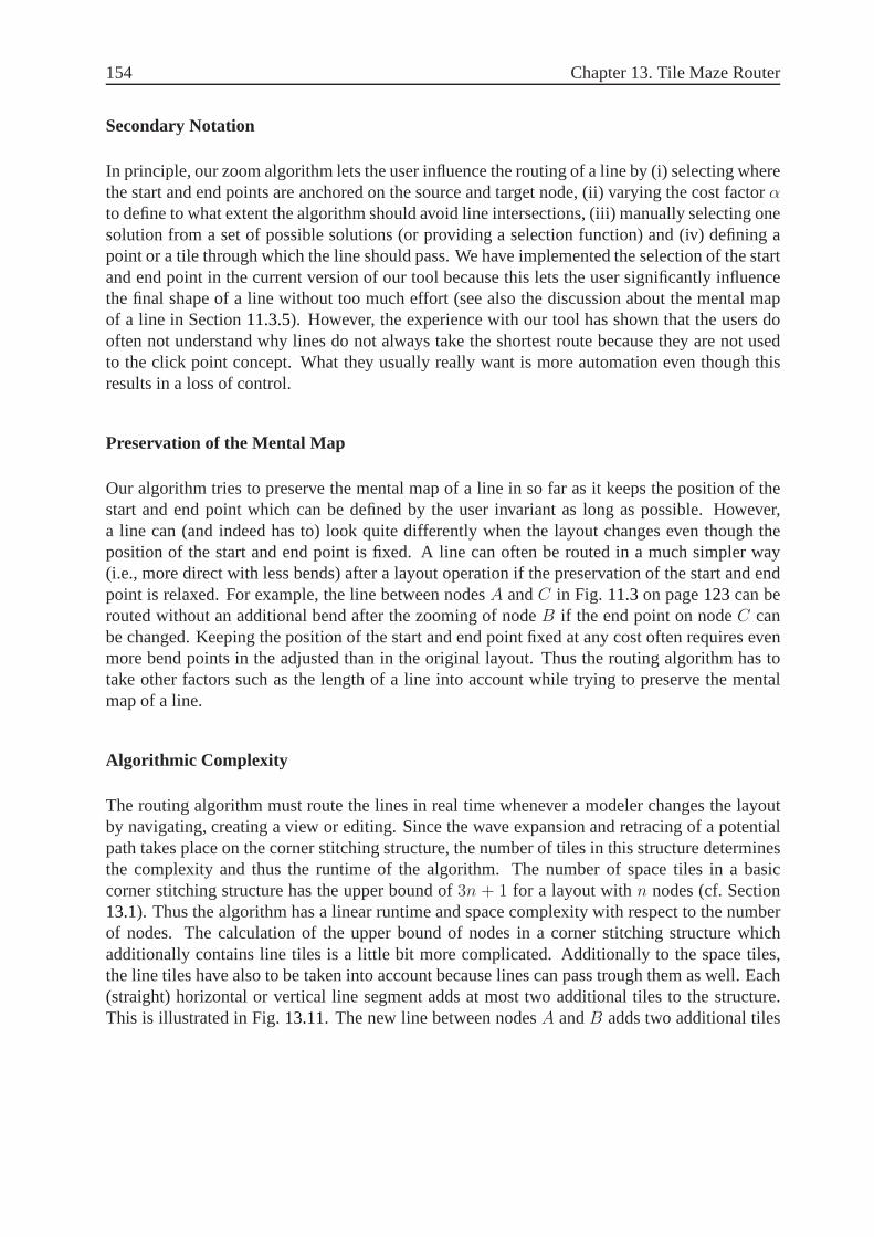
154 Chapter 13. Tile Maze Router
Secondary Notation
In principle, our zoom algorithm lets the user influence the routing of a line by (i) selecting wherethe start and end points are anchored on the source and targetnode, (ii) varying the cost factorαto define to what extent the algorithm should avoid line intersections, (iii) manually selecting onesolution from a set of possible solutions (or providing a selection function) and (iv) defining apoint or a tile through which the line should pass. We have implemented the selection of the startand end point in the current version of our tool because this lets the user significantly influencethe final shape of a line without too much effort (see also the discussion about the mental mapof a line in Section11.3.5). However, the experience with our tool has shown that the users dooften not understand why lines do not always take the shortest route because they are not usedto the click point concept. What they usually really want is more automation even though thisresults in a loss of control.
Preservation of the Mental Map
Our algorithm tries to preserve the mental map of a line in so far as it keeps the position of thestart and end point which can be defined by the user invariant as long as possible. However,a line can (and indeed has to) look quite differently when thelayout changes even though theposition of the start and end point is fixed. A line can often berouted in a much simpler way(i.e., more direct with less bends) after a layout operationif the preservation of the start and endpoint is relaxed. For example, the line between nodesA andC in Fig. 11.3on page123can berouted without an additional bend after the zooming of nodeB if the end point on nodeC canbe changed. Keeping the position of the start and end point fixed at any cost often requires evenmore bend points in the adjusted than in the original layout.Thus the routing algorithm has totake other factors such as the length of a line into account while trying to preserve the mentalmap of a line.
Algorithmic Complexity
The routing algorithm must route the lines in real time whenever a modeler changes the layoutby navigating, creating a view or editing. Since the wave expansion and retracing of a potentialpath takes place on the corner stitching structure, the number of tiles in this structure determinesthe complexity and thus the runtime of the algorithm. The number of space tiles in a basiccorner stitching structure has the upper bound of3n + 1 for a layout withn nodes (cf. Section13.1). Thus the algorithm has a linear runtime and space complexity with respect to the numberof nodes. The calculation of the upper bound of nodes in a corner stitching structure whichadditionally contains line tiles is a little bit more complicated. Additionally to the space tiles,the line tiles have also to be taken into account because lines can pass trough them as well. Each(straight) horizontal or vertical line segment adds at mosttwo additional tiles to the structure.This is illustrated in Fig.13.11. The new line between nodesA andB adds two additional tiles
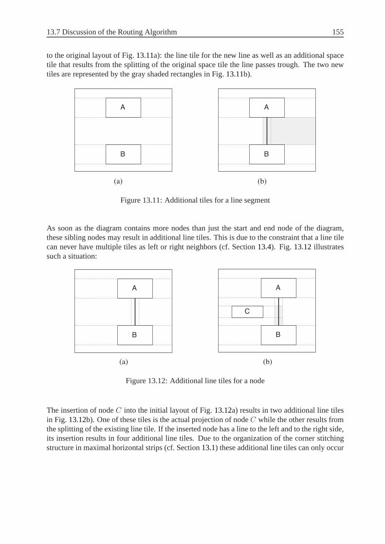
13.7 Discussion of the Routing Algorithm 155
to the original layout of Fig.13.11a): the line tile for the new line as well as an additional spacetile that results from the splitting of the original space tile the line passes trough. The two newtiles are represented by the gray shaded rectangles in Fig.13.11b).
A
B
A
B
(a) (b)
Figure 13.11: Additional tiles for a line segment
As soon as the diagram contains more nodes than just the startand end node of the diagram,these sibling nodes may result in additional line tiles. This is due to the constraint that a line tilecan never have multiple tiles as left or right neighbors (cf.Section13.4). Fig. 13.12illustratessuch a situation:
A
B
C
A
B
(a) (b)
Figure 13.12: Additional line tiles for a node
The insertion of nodeC into the initial layout of Fig.13.12a) results in two additional line tilesin Fig. 13.12b). One of these tiles is the actual projection of nodeC while the other results fromthe splitting of the existing line tile. If the inserted nodehas a line to the left and to the right side,its insertion results in four additional line tiles. Due to the organization of the corner stitchingstructure in maximal horizontal strips (cf. Section13.1) these additional line tiles can only occur

156 Chapter 13. Tile Maze Router
in vertical line segments. However, as a simplification so that we do not have to distinguishbetween vertical and horizontal line segments and because we are looking for an upper bound,we can state that each node can result in four additional linetiles.
Fig. 13.13shows that each bend (i.e., transition from a horizontal to avertical segment or viceversa) results in one additional line tile (the gray shaded rectangle). The other line tiles resultfrom the two line segments and from nodeA that splits the line tile representing the vertical linesegment. Since a line tile has a minimal width3 the tile representing the bend is never split.
A
B
(a) (b)
A
B
Figure 13.13: Additional line tiles for a bend
As soon as lines intersect, each such crossing results in at most three additional line tiles. AsFig.13.14illustrates, one of these additional tiles represent the intersection point itself, while theother two result from the splitting of the two line tiles representing the crossing lines.
A
B
(a) (b)
C D
B
C D
A
Figure 13.14: Additional line tiles for line crossing
3The width of the line tiles in the figures is that large only forillustrative purposes. Line tiles are actually onlyone unit wide.

13.7 Discussion of the Routing Algorithm 157
Taking all these situations into account yields the following formula for the calculation of theupper boundt of tiles that are relevant for the routing of a line in a line tile structure:
t = 7n+ 3c+ 2s+ b (13.5)
wheren is the number of nodes,c the number of crossings between existing lines,s the number of(straight) line segments all existing lines consist of andb the number of all bend points in existinglines. While this gives the upper limit for the number of nodes a corner stitching structure canconsist of, the number of tiles that are actually visited during the wave expansion and retracingphases of the routing algorithm is much lower. First of all, the hierarchical nesting of nodesresults in a number of smaller corner stitching structures containing only a fraction of the nodesand links of the diagram instead of one big structure that contains all nodes and links. Each lineuses its own corner stitching structure that contains only the nodes and links that are, becauseof their position in the hierarchy, relevant for it (cf. Sections11.1and13.1). Furthermore, dueto the directed search employed in the wave expansion phase of the routing algorithm most ofthe time only a fraction of the tiles have to be visited until the target is reached. A rudimentaryanalysis of the line routing in three case studies4 has revealed that in the average only 50-60%of the “routable” tiles (i.e., space and line tiles) are actually visited during the wave expansion.Existing lines increase the number of tiles but at the same time line tiles act as barriers baring thewave from propagating and thus reducing the overall effort of the routing algorithm. The averagelength of the tile paths that result from the retracing phaseis also very low in the case studies asmost of them consisted of three or less tiles so that the bend point calculation can be done veryquickly.
4The case studies were the mine drainage and elevator system used for the experimental validation of the fisheyezoom (cf. Section16.1) plus one real industrial case study, a model of a license management system consisting of125 nodes and 108 links.


159
CHAPTER 14
Line Labels
A problem that is closely related to the line routing is the placement of labels that accompanylines. While line labels are not of much importance in abstract graphs, they often contain a bigpart of the information represented in a graphical model. For example, transition descriptionsin statecharts [Harel, 1987] or ADORA models (cf. Section4.1) contain a large part of the infor-mation represented in a diagram. Because of this large amount of information, line labels canhave a significant size. This goes somewhat against the nature of node-link diagrams in whichlinks only connect entities (the nodes) and are usually not seen as entities themselves. Somenotations such as the Specification and Description Language (SDL) [ITU-T, 2000] address thisrepresentation mismatch by using a set of nodes (e.g., Input, Output, Procedure) instead of a linkaccompanied by a big label to describe a state transition. Incontrast, the Requirements StateMachine Language (RSML) [Leveson et al., 1994] represents state transitions by a simple arrowbetween two states and describes them externally to the diagram in a mixed textual/tabular nota-tion. While this approach avoids the label problem almost completely as there are no transitionlabels anymore, it also removes one of the biggest advantages of a graphical state-based notation,namely the possibility to see the whole specification with one glance. Another possibility to re-duce the number of line labels and thus potential problems with them is to show and hide themon demand or to show most of the information in a tool tip whichpops up on close inspection ofa line only.
Since the characteristics of (big) line labels are similar to those of nodes, the same problemsof overlaps occur. Labels can overlap with existing nodes and/or other labels. These overlapsimpede the readability of the diagram. Additionally, an inappropriate position of a line labelclose to other links can make it hard to determine the line it belongs to. Thus, deciding on the

160 Chapter 14. Line Labels
position of a line label entails not only finding enough whitespace to avoid overlaps but alsoselecting an appropriate position relative to the line. Additionally, the position of a label relativeto the line is often part of the secondary notation (cf. Section 2.5). For example, the position ofassociation labels in UML (cf. Section2.2.2) relative to the start and end node determines theassociation’s direction they describe.
The dynamic layout that results from the use of a fisheye zoom (cf. Chapter7) or view generationalgorithm (cf. Chapter8) intensifies the problem of overlapping labels. Labels can suddenlyoverlap after a layout adjustment. Fig.14.1shows an example. The label of the line betweennodesB andC does not overlap with any other element in the original layout of Fig. 14.1a). Inthe layout that results from zooming out nodeA the label overlaps with nodesB andC becausethe zoom algorithm has moved the two nodes closer together asshown in Fig.14.1b).
(a)(b)
D
A
B Creceive check() |
send valid()
A...
B Creceive check() |
send valid()
Figure 14.1: Overlapping label after zooming-out node A
14.1 Label Placement Rules
The problem of associating graphical features with text labels has applications in many fieldssuch as graph drawing and cartography. Cartographers have been using rules for a good place-ment of labels over centuries. These rules can be used as a basis for an automatic label placementalgorithm. For the problem of placing line labels in a diagram the following rules can be derivedfrom the basic rules for placing labels on geographic maps [Imhof, 1975; Yoeli, 1972]:
1. Line labels mustnot overlapwith other labels or other graphical features of the layout.
2. Each label can be easilyidentified with exactly one line(i.e., the assignment of a label to aline is unambiguous).
3. Each label must be placed in thebest possible position(among all acceptable positions).The best possible position is usually defined by a set of aesthetic preferences such as thata label to the right is always preferred over one to the left ofa symbol.

14.2 Basic Approaches 161
For diagrams that employ the nested set notation (cf. Section 3.3.1) an additional rule has to beadded:
4. Each labels must befully containedwithin the parent node of the line it belongs to. Theparent node of a line is defined as the first common ancestor of the line’s source and targetnode.
14.2 Basic Approaches
Algorithms to place1 line labels can be classified according to the degree they influence or changethe overall layout of a diagram. Approaches can range from the movement of nodes and thussignificant changes of the layout to minimal invasive approaches which take the layout (i.e.,position and size of the nodes) as well as the routing of the lines as given constraints.
14.2.1 Adjusting the Layout
The basic idea of a label placement algorithm that is integrated into a layout algorithm is to adjustthe layout (i.e., position and size of the nodes) in order to get the space required by the line labels.One solution could be to use the zoom algorithm of chapter7 to resolve overlaps between linelabels and nodes or among line labels. This seems to be a straightforward approach since thezoom algorithm has been designed to avoid or resolve overlaps between nodes. Fig.14.2showshow this technique can be applied to the situation shown in Fig. 14.1b) to resolve the overlaps.NodesB andC have been moved away from each other in order to provide the space requiredby the label.
A...
B Creceive check() |
send valid()
Figure 14.2: Move nodesA andB to provide the required space to the label
However, this approach has three drawbacks. First, the additional layout changes that occurduring the label placement can easily destroy the secondarynotation and the user’s mental mapof a diagram (cf. Sections2.5and5.3). Second, it can become difficult to maintain the stability of
1We use the term label “placement” not only for the calculation of a label’s position but for the definition of itsboundaries (i.e., positionandsize) in general.

162 Chapter 14. Line Labels
the zoom algorithm (cf. Section5.4) if line labels have an influence on the layout. For example,if the user zooms a node in and then out again, the resulting layout changes have to be undone.This can become rather difficult if the layout is changed in between to provide additional spaceto line labels. And third, as shown in Section11.2, the layout adjustments done by the zoomalgorithm often demand for a different routing of a line eventhough the overall layout has notchanged dramatically. To handle such situations, we have separated the line router from thezoom algorithm so that the line router adjusts the lines after the zoom algorithm has adjusted thelayout. If the zoom algorithm is additionally responsible for adjusting the position of line labels,it tries to keep their relative position to the surrounding nodes in order to preserve the mentalmap. If a line is then routed again, the position of accompanying labels and the line often do notmatch anymore. Using the zoom algorithm to place labels has an influence on how the line isrouted afterwards (because it changes the layout and thus the position and/or size of the nodeswhich determines the route of the line). This routing has again an influence on where the labelshould be placed (as the line and the label should be close together). Thus, coupling the zoomand routing algorithm by using the zoom algorithm to place line labels lets them influence oneanother which may result in an oscillating layout. An additional, more technical advantage ofseparating the routing and label placement algorithm from the zoom/layout algorithm is that theycan be used and maintained independently.
14.2.2 Influence the Line Routing
A little less invasive is the idea to integrate the placementof labels into the line routing algorithm.Such an integration employs two different ideas: First, to integrate existing, already placed linelabels (i.e., those belonging to lines which have already been routed) into the routing algorithmso that they are not crossed by newly added lines. This can be achieved by treating line labels ina similar way as existing lines in our routing algorithm (cf.Section13.4). And second, to let therouting algorithm look for another solution if the current route of a line does not provide enoughspace for the associated labels. Fig.14.3illustrates how the line between nodesB andC can berouted to avoid the overlaps shown in Fig.14.1b):
A...
B C
receive check() |
send valid()
Figure 14.3: Reroute the line to provide the required space to the label

14.3 Tile-based Label Placement 163
The biggest problem of this approach is that it can influence the line significantly and thus makeit harder to fulfill some of the desired properties for the line routing, such as the minimal lengthof a link (cf. Section11.3.2). On the other side, the interferences with the secondary notationand the mental map are much less severe than for the integration of the label placement into thezoom algorithm because lines are usually seen as less crucial than nodes for the preservation ofthe mental map (cf. Section11.3.5).
14.2.3 Layout and Line Routing as Constraints
The most conservative label placement strategy is to place the labels without changing anythingof the existing layout of nodes and lines. Overlaps between labels and nodes or among labels canbe avoided by adjusting the labels’ position and size only. Thus, the label placement algorithmworks on a fixed geometry. While such an approach minimizes the influence on the user’s mentalmap and secondary notation, it also constrains the freedom of the label placement algorithm.The chance that the algorithm cannot place a label without any overlaps is significantly higherthan with the other approaches. However, this problem can bemitigated if the model is createdinteractively by the user as he can influence and thus improvethe label placement by adjustingthe layout himself.
The cartography field has to deal with similar label placement problems: While the “node labelplacement problem” deals with the labeling of points in the plane so that no labels overlap pointsor other labels, the “edge label placement problem” is concerned with the assignment of textlabels to edges such that the quality of the assignment is optimal. Even though the label place-ment problem is NP-hard and essentially unsolved [Kakoulis and Tollis, 1997], a large numberof heuristic approaches have been developed (see e.g. [Christensen et al., 1995] for a survey ofalgorithms for the labeling problem). While these algorithms use optimization techniques suchas discrete gradient descent or simulated annealing to find aglobal optimum, such techniquescannot be used for an interactive modeling tool because the runtime of a label placement algo-rithm is a critical factor as a potentially very large numberof labels have to be placed without aremarkable delay.
14.3 Tile-based Label Placement
The corner stitching structure which is the basic data structure of our routing algorithm (cf. Sec-tion 13.1) can be reused for a simple label placement algorithm. Because the general label place-ment problem is NP-hard, the presented approach is a heuristic which does not always result inan optimal solution. Furthermore, because a graphical model is usually created incrementallyby the user adding one element after the other, the presentedtechnique is also incremental. Thelabels that belong to a line are placed whenever this line is routed and the label placement algo-rithm works within a fixed geometry defined by the nodes, previously routed lines and the labels

164 Chapter 14. Line Labels
which belong to previously routed lines. Thus, already placed labels are not repositioned in orderto reach a global optimum like in other labeling algorithms such as [Christensen et al., 1995] or[Kakoulis and Tollis, 1997]. The presented algorithm has already been published in [Reinhardand Glinz, 2010].
The basic idea of the label placement approach is to use the corner stitching structure to calculatethe white space that can be used to place line labels. This calculation is trivial because the emptyspace is explicitly represented in the corner stitching structure (cf. Section13.1). The whitespace calculation avoids overlaps of line labels with nodes, existing lines (if they are explicitlyrepresented in the corner stitching structure as shown in section13.4) and existing line labels (ifthey are represented in the structure in similar way as existing lines). Additionally, the use ofthe corner stitching structure results in labels that are always contained within the line’s parentnode. A set of potential label positions with a predefined relative position to the line is thencalculated within this white space. Among these candidate positions the best one with respect tosome predefined criteria is selected. The detailed steps of the algorithm are the following:
1. Iterate over all (vertical and horizontal) line segments.
2. Use the corner stitching structure to calculate the available free space around the segment:First a reference point for each label is defined. This point can either be the midpoint ofthe segment if the label should be shown on the middle of the line or the segment’s startor end point. The corner stitching structure is then used to find the tile this reference pointlies in (cf. Section13.1for the detailed algorithm to find a tile at a given location).Finally,the free space is calculated by vertically extending the boundaries of the tile containingthe reference point. Fig.14.4shows an example of this step.P1 andP2 are the referencepoints for the two line segments of the line connecting nodesA andB.
A
B
2
1
P1
P2
Figure 14.4: Calculation of the label space on the corner stitching structure

14.3 Tile-based Label Placement 165
The corner stitching structure for this constellation is shown by the dashed lines. Thehatched areas1 and 2 show the free space that has been calculated forP1 andP2 re-spectively. In our current implementation the width of the free space for horizontal linesegments is restricted to the length of the segment (as shownfor the hatched area1 inFig. 14.4). The vertical expansion of the free space stops as soon as the width of the nexttile above or below is smaller than the current width of the white space. That’s why theexpansion of the free space2 stops below nodeA and above nodeB.
3. Determine three candidate positions for each line segment: For a horizontal segment theseare above, below and vertically centered around the reference point. For a vertical segmentthey are to the left, the right and vertically centered around the reference point.
Fig. 14.5shows the six candidate positions for a line label that belongs to the line betweennodesA andB. In our current implementation the label is asked for its required heightgiven a specific maximal width. This maximal width is directly taken from the width ofthe free space adjusted by the relative position of the label(i.e., the maximal width of label6 in Fig. 14.5is the width of the free space to the right of the second line segment). This isa very basic approach which tries to make labels as wide as possible. Other more sophisti-cated approaches that take for example the content of the label into account to calculate itsboundaries can easily be implemented as part of the label’s internal size calculation with-out changing the placement algorithm. For example, in ADORA models such an approachcould always try to write each of the components of a transition description on a separateline.
A
B
4 56
2
3
1
Figure 14.5: Candidate label positions
4. Select one of these candidates: To do so we associate a score with each candidate position.This score combines a set of a priori preferences with a valuethat reflects the severityof the violation of the basic label placement rules (1) and (2) of section14.1. The basiclabel placement rules can be violated if there is not enough space for the label at the given

166 Chapter 14. Line Labels
position so that it overlaps with nodes (or other labels) or if the label is crossed by the lineit belongs to.
For the example of Fig.14.5, the algorithm selects label position1 if it prefers labels abovehorizontal segments or position4 if it prefers labels to the left of vertical segments. Thescoring can, together with a specific reference point, also be used to prefer positions closeto the source or target node if such a position is an importantpart of the secondary notation.
Discussion
The implementation of the presented label placement algorithm is in its basic form straightfor-ward as a large part of the logic lies in the corner stitching structure. As a proof-of-concept, itshows that it is possible to use the corner stitching structure, originally used for the line routing,for the placement of labels too. Much more sophisticated approaches can be built on top of thisbasic idea. The three main extension points are the calculation of the white space (e.g., calcu-lating the free space for each candidate position independently), the calculation of the candidatepositions (e.g., using multiple reference points or different label boundaries for each segment)and the scoring of the candidate positions. However, already the presented simple approach canmitigate the label problem to a large extend even though it may not always find the “best” positionfor a label. Fig.14.6shows how our current implementation solves the problem of overlappinglabels after a zoom operation as shown in Fig.14.1by adjusting the boundaries of the label:
A...
B C
receive
check() |
send
valid()
Figure 14.6: Solution for Fig.14.1

Part IV
Validation


169
CHAPTER 15
Constructive Validation
The basic goal of the work presented in this thesis is to show that the visualization concepts thatare an integral part of the ADORA modeling approach can be realized and made to work in a basicimplementation. Thus, their implementation in a working tool and use on models of realistic sizeconstitute an important part of the validation. While Chapters10, 13.7and14.3discuss technicalaspects of the zoom, line routing and label placement algorithms and data structures in order toshow that the presented concepts work and have some desired properties, this chapter gives ashort overview over their actual implementation in the ADORA tool.
15.1 Layout Functionality
We use the model of a simple elevator control system to illustrate how the ADORA tool supportsthe modeler in editing and navigating through a model. This model is the same as the one usedfor our experimental validation (cf. Chapter16). It is shown with all views enabled and all nodeszoomed in by Fig.A.2 on page195. Even though the model is with its 67 nodes and 63 linksstill of reasonable size, it can easily be seen in Fig.A.2 that it already becomes impractical toshow (and especially print) the whole diagram with all elements at once. As a consequence, thescreenshots in the following sections show only a subset of the elements in the model. However,the underlying model is the complete one, so that the diagramlooks exactly like the one inFig. A.2 if the user zooms in all nodes and enables all views. The usefulness of the screenshotswould be rather limited without the complexity management mechanism employed by the fisheyezooming and dynamic view generation implicitly being used all the time.
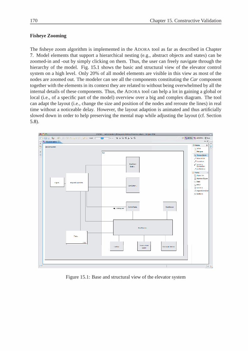
170 Chapter 15. Constructive Validation
Fisheye Zooming
The fisheye zoom algorithm is implemented in the ADORA tool as far as described in Chapter7. Model elements that support a hierarchical nesting (e.g.,abstract objects and states) can bezoomed-in and -out by simply clicking on them. Thus, the usercan freely navigate through thehierarchy of the model. Fig.15.1 shows the basic and structural view of the elevator controlsystem on a high level. Only 20% of all model elements are visible in this view as most of thenodes are zoomed out. The modeler can see all the components constituting theCar componenttogether with the elements in its context they are related towithout being overwhelmed by all theinternal details of these components. Thus, the ADORA tool can help a lot in gaining a global orlocal (i.e., of a specific part of the model) overview over a big and complex diagram. The toolcan adapt the layout (i.e., change the size and position of the nodes and reroute the lines) in realtime without a noticeable delay. However, the layout adaption is animated and thus artificiallyslowed down in order to help preserving the mental map while adjusting the layout (cf. Section5.8).
Figure 15.1: Base and structural view of the elevator system

15.1 Layout Functionality 171
15.1.1 Dynamically Generated Views
A separation of concerns is achieved by letting the user disable or enable any of the views of theADORA language (except for the base view which is shown all the time). Views are enabled ordisabled globally (e.g., all states and transitions becomevisible if the behavior view is enabled).However, the final appearance of a diagram results from combining the view concept with thefisheye zoom because model elements that are located within azoomed-out node do not becomevisible even if the view they belong to is enabled. The ADORA tool relies on the conceptspresented in Chapter8 to adjust the layout if model elements are shown or hidden according tothe selected view(s). Fig.15.2shows again the same model but this time with the focus on thebehavior of theUpButtonwithin theFloor’s ControlPanelcomponent.
Figure 15.2: Behavior view with focus on the UpButton
To produce this view, the user has enabled the behavior view and zoomed out the neighboringnodes. The diagram in Fig.15.2is still compact and concise even though it is a very detailedviewas it shows the formal transition description and is thus on the same level as the program code.In contrast to other modeling tools, the description of the behavior of theUpButtonis shownin the context of this component. As a consequence the user isalways aware of the context ofthe component she is currently working on (e.g., theUpButtonin theControlPanelof a Floor).Additionally, some of the elements in the context have a direct influence on the behavior of

172 Chapter 15. Constructive Validation
the UpButtonwithin the context of the elevator system. For example, the transition from theactivatedto the inactivestate is triggered by an event which is sent over the communicationchannel betweenRequestDispatcherandUpButton. The user can now further investigate thecollaboration between these two components by zooming intotheRequestDispatcherto find outwhere exactly the triggering event is produced. The transition between different diagrams thatresult from the enabling of different views is animated to increase the continuity.
15.1.2 Editing Support
The nested node notation employed by the ADORA language to represent the hierarchical de-composition increases the need for tool support because a change in one part of the model ispropagated upwards through the hierarchy to the root node. For example, the user has to expandall direct and indirect parents of a node to provide the spacethat is required by a new node. Inorder to make the nested node notation usable without any overhead, the ADORA tool automat-ically expands ancestor(s) if more space is required after anode has been inserted or moved byusing the mechanism presented in Chapter9. Conversely, parent node(s) are contracted automat-ically by the tool if a node is removed. This editing support of the the ADORA tool is illustratedin Fig. 15.3.
Figure 15.3: Inserting a new node

15.1 Layout Functionality 173
The insertion of a new component into theUpButtoncomponent of the initial layout of Fig.15.2expands all the ancestors of this node in order to provide therequired space. This layout adjust-ment tries to preserve the original layout as far as possibleso that the user still recognizes thediagram.
15.1.3 Line Routing and Label Placement
Lines are routed completely automatically by the tool (as described in Chapter13) to unbur-den the user from this tedious task which has to be performed after each change in the layout.Such layout changes occur frequently because of the fisheye zooming and the dynamically gen-erated views. Furthermore, abstract associations (cf. Section 11.1) are calculated automaticallywhenever at least one of the direct or indirect parents of a line’s source or target node is zoomed-out. The user has some influence on how a line looks like by locating the start and end pointof a line. Furthermore, labels attached to the lines are placed automatically (cf. Chapter14).Fig. 15.4shows the resulting layout after a link betweenDirectionIndicatorandFloorDoor hasbeen added to the layout of Fig.15.3:
Figure 15.4: Automatic line routing and label placement
The link avoids the obstacle (i.e., theControlPanelcomponent) between its start and end nodewhile staying within the boundaries of the common ancestor of the start and end node (i.e., the

174 Chapter 15. Constructive Validation
Floor component). The alternative route around the top boundary of the ControlPanelhas beendiscarded during the routing as it would have crossed two existing links. Fig.15.4also illustrateshow the alternating shading of nodes (cf. Section3.3.1) helps in distinguishing links from nodeboundaries. The label that accompanies the new link has beenplaced at the position providingthe most empty space. Changing the horizontal position of the link’s start point within theDi-rectionIndicatorcomponent (which has been defined by the user by clicking on the appropriateposition within the node) can change the label’s position when the empty space at its currentposition shrinks.
15.2 Technical Aspects
Even though we used the ADORA language and tool as an example to show how the conceptspresented in this thesis can be used on an integrated modeling language, the concepts themselvesare independent of any specific language. Their implementation in the ADORA tool is a proofof concept. The only language or more precisely representation concept that is required by thefisheye zoom is the nested node notation (cf. Section3.3.1). The routing algorithm relies only onthe basic concept of node link diagrams (cf. Section2.1.3). These requirements of the zoom androuting algorithm on nodes and links are described in a few simple Java interfaces. The fisheyezoom and line routing components are decoupled from the coreof the ADORA tool so that theycan be used in other environments too. The code base of the twocomponents is rather small:The zoom component has roughly 5200 TLOC (+ 4800 TLOC of unit tests) and the line routingcomponent has 2900 TLOC (+ 3600 TLOC in tests).

175
CHAPTER 16
Experimental Validation
While the focus of the last chapter lies on the implementation of the presented concepts and al-gorithms in order to show that they do work on models of realistic size, this chapter examinesthe overall usefulness of the presented approach. We have conducted a small controlled exper-iment (i.e., a classroom experiment with students) to investigate the use of the fisheye zoomtechnique. The influence of our line routing technique (cf. Part III ) was not addressed explicitlyduring the experiment. However, it was implicitly part of the experiment as all lines were routedautomatically with the presented technique during the experiment.
16.1 Experiment
The aim of our experiment was twofold: First, to compare the performance of using a graphicalmodel with a fisheye zoom with the one of using a fully expandedmodel to find out whetherthere are any significant differences. And second, to observe how exactly the subjects use thefisheye zoom (i.e., which zoom operations are executed in which order). We did not compare thefisheye zoom with an explosive zoom because (i) this comparison has already been done [Schaf-fer et al., 1993, 1996] and (ii) some constructs of our technique such as abstract relationships(cf. Section11.1) cannot be used in combination with an explosive zoom. Additionally, a fullyexpanded model makes a stronger benchmark for a comparison since the mental integration ofdifferent models, which is the biggest drawback of an explosive zoom, does not apply. The ma-jor drawback of comparing our fisheye zoom to a fully expandedmodel instead of the traditionalexplosive zoom is that it almost certainly results in much less significant results than for example

176 Chapter 16. Experimental Validation
the experiments ofSchaffer et al.[1996].
The test subjects were asked a set of dual- and multiple-choice questions about shown models.They were split into two groups of which one group had to answer a set of questions about amodel using the fisheye zoom while the other group had to answer the same questions about thesame model without the possibility to use the fisheye zoom (i.e., without the possibility to openand collapse nodes). The roles were then exchanged so that the first group used a fully expandedmodel without the possibility to zoom while the second grouphad to use the fisheye zoom toanswer the questions about a second model.
The two factors efficiency and effectiveness were used to evaluate the performance. The ef-ficiency was determined by measuring the time used to answer aquestion. We define the ef-fectiveness by whether, or more precisely to which degree, agiven answer was correct. Wecombined the two factors in order to judge the performance byusing the ratio between efficiencyand effectiveness which gives us the number of correct answers per time unit1. We use the termperformance points for the resulting value.
Performance points=Correctness in %
Required time in seconds
Correctness lies somewhere between 0% and 100% for multiple-choice questions and is 0% or100% for single-choice questions. The testing environmentensured that the user always selectedat least one of the given answers so that the situation of not answering a question did not occur. Inaddition to these objective questions, the subjects were also asked a set of subjective questions.
Hypothesis
Our null hypothesis was that there exists no difference in performance (withp = 0.05) betweensubjects using our fisheye zoom and those using the fully expanded model. The performance ofthe subjects was measured by calculating the performance points as described above.
Case Studies
We used two independent case studies for the experiment. Both of these case studies must havesimilar size and complexity. A subset of the ADORA language (cf. Section4.1) was used asnotation for the models because we have implemented our zoomalgorithm as part of the ADORA
tool (cf. Section4.2). Only the base, structural and behavior views of ADORA have been usedin the experiment to reduce the impact of the language and thenotation on the results. The twocase studies were the mine drainage and the elevator system.
1We follow here the approach of [Meier, 2009].

16.1 Experiment 177
Themine drainage systemconcerns the software necessary to manage a simplified pump controlsystem for a mining environment. The pump is used to pump minewater, which collects at thebottom of a shaft, to the surface. The main safety requirement is that the pump must not operatewhen the level of methane gas in the mine reaches a critical value due to the risk of explosion.Additionally, the system must measure the level of carbon dioxide in the air and detect whetherthere is an adequate flow of air. An alarm must be activated if the carbon dioxide level or airflowbecome critical. The mine drainage system case study is widely used in the software engineeringfield and goes back toKramer et al.[1983]. The model is shown in Fig.A.1 as part of AppendixA. It consists of 55 nodes (14 components and 41 states) and 63 links (13 associations and 50transitions).
The second case study, theelevator system(which was originally introduced byFilman andFriedman[1984]), comprises the control software of a simple single car (cabin) elevator system.Parts of the system are the different operation units in the car and on the floor as well as thecontrol of the door mechanism and the motor. Fig.A.2 in AppendixA shows the model of theelevator system that was used for the experiment. The model of the elevator system contains 67nodes (33 components and 34 states) and 63 links (19 associations and 44 transitions).
Test Environment
The ADORA tool (cf. Section4.2) that was used for the experiment facilitates inquiries with abuilt-in electronic questionnaire. The model(s) the user interacts with and the correspondingquestions are shown together at the same time. The given answers and the time needed to answera question are recorded in a database which can subsequentlybe used to analyze the results. Thescreenshot of Figure16.1shows a question in the left panel together with the model that has tobe used to answer the question in the center.
Questionnaire
The complete questionnaires for the mine drainage and elevator system can be found in sectionsA.2.2 andA.2.3 respectively. The questionnaires incorporate three kindsof questions: First,the subjects where asked about their gender and for a self-assessment of their modeling skills.Second, they had to answer a set of objective questions aboutthe shown models. About halfof these questions concerned only the semantics of nested node-link diagrams (e.g., whethertwo nodes are connected or which nodes are contained within aspecific node). The other halfconcerned the ADORA execution semantics (e.g., which events are fired or the states a componentis in after a set of events have occurred). The required operations to answer the questions weretypical task to explore a graphical model. They were restricted to navigating through the modelwithout doing any modifications. At the end of the experiment, the subjects had to judge withtheir subjective opinion the usefulness of the fisheye zoom and an (optional) linear zoom.

178 Chapter 16. Experimental Validation
Figure 16.1: Screenshot of the empirical testing environment
Organization
The experiment started with a 25 minute introduction of the relevant constructs of the ADORA
language, the ADORA tool as well as the experiment itself. The subjects then started the ex-periment by answering two introductory questions: their gender and their modeling skills. Sub-sequently, they had to answer a first set of 15 questions aboutthe mine drainage system. Thefirst group had to use the fisheye zoom while answering these questions, while the second group(i.e., the control group) had to answer the questions using the fully expanded model. A set of 15questions about the elevator system followed with the rolesof the two groups exchanged. Thefirst group was now the control group using the fully expandedmodel while the second grouphad to use the fisheye zoom. At the end both groups had to subjectively judge the usefulness ofthe fisheye zoom and an optional linear zoom in answering the questions. The answers and thetime required were gathered automatically for all subjects. The subjects required between 22 and45 minutes to answer the 34 questions.

16.2 Results 179
Subjects
We conducted the experiment with eight (one female and sevenmale) students simultaneouslyat one date as part of a requirements engineering master course at the University of Zurich. Thesubjects had no or only little experience with the ADORA language. Seven subjects rated theirgeneral modeling skills in a self-assessment as medium (i.e., selected the answer “I use modelingtechniques from time to time.”) while one assessed his/her modeling skills as high (i.e., selectedthe answer “I am experienced.”). As a preliminary preparation they had to read the papers [Glinzet al., 2002, 2007; Meier et al., 2006] and to model a small case study [Davies et al., 2001] inthe ADORA language using the ADORA tool. Before the actual experiment started, they wereadditionally given a short introduction on those parts of the language and the tool which wererelevant for the experiment. The subjects were then randomly and equally distributed among twogroups. The experiment was conducted anonymously in order to avoid biased answers.
16.2 Results
The raw results (i.e., correctness of the answers and time needed) for each individual subject canbe found in tablesA.1 andA.2 in the appendix. Fig.16.2and16.3show the resulting perfor-mance points as box plots for the mine drainage and the elevator system. The gray boxes showthe results for the group that used the fisheye zoom while the white boxes show the performanceof the control group. A direct comparison makes only sense within a question and not betweenquestions because there were different kinds of questions (i.e., employ different tasks which hasan influence on the results [Büring et al., 2006; Gutwin and Fedak, 2004]). For example, thetime required to answer question Q15 which involved the examination of the interplay betweenmultiple components and connections was significantly larger than the one to answer questionQ6 (a simple listing of all components contained within a specific component). This results inlarge differences in the achieved performance.
Statistical Analysis
We conducted a simple unpaired2 t-test with an error probability of 5% to check whether the meanof the subjects that used the fisheye zoom is distinct from theone of the subjects that worked withthe fully expanded model. We applied the test to each question separately to find out whether theoutcome depends on the kind of task that a specific question employs. The results of the statisticalanalysis can be found in tablesA.3 andA.4 in the appendix. The only statistically significantdifference between using the fisheye zoom and working on a fully expanded model occurs inquestion Q20 concerning the elevator system (i.e., we couldonly reject our null hypothesis for
2We actually have paired questions for the mine drainage and elevator system (e.g., questions Q3 and Q18demand the same task) but cannot use a paired t-test since themodels are not the same.

180 Chapter 16. Experimental Validation
0
1
2
3
4
5
6
7
Q1 Q2 Q3 Q4 Q5 Q6 Q7 Q8 Q9 Q10 Q11 Q12 Q13 Q14 Q15
Figure 16.2: Performance points for the mine drainage system
question Q20). The control group performed significantly better than the group using the fisheyezoom while answering this specific question. The subjects had to search the whole model for aspecific node and indicate the component this state lies in. The group using the fisheye zoomhad to open (and close) a large fraction of all nodes in the model which gives an explanationfor its bad performance (see also the detailed analysis of the interaction below). Interestingly,no significant difference has been found for Q5, the equivalent question for the mine drainagesystem.
Subjective Questions
At the end of the experiment the subjects were asked in two questions (Q31 and Q32) to subjec-tively judge the usefulness of the fisheye zoom and a traditional global (linear) zoom in answeringthe objective questions. Six of them stated that the fisheye zoom makes it easier to answer thequestions while two selected the answer that it makes it easier in some cases. The answers weremore diverse for the global zoom: Half of the subjects did notuse it at all (i.e., they navigated thefully expanded model by panning only). Two selected the answer that the global zoom makes iteasier in some cases to answer the questions, one that it doesnot have any influence and one thatit makes it more difficult to answer the questions.

16.2 Results 181
0
2
4
6
8
10
12
14
16
Q16 Q17 Q18 Q19 Q20 Q21 Q22 Q23 Q24 Q25 Q26 Q27 Q28 Q29 Q30
Figure 16.3: Performance points for the elevator system
Analysis of the Subjects’ Interaction
The automatic recording of all zoom operations (together with a time stamp) facilitates a detailedanalysis of how exactly the subjects used the fisheye zoom. Additionally, it helps in understand-ing and explaining the results of the statistical analysis.Fig. 16.4shows a graphical represen-tation of the interaction of one of the subjects with the minedrainage system. The progress oftime in seconds is shown on the horizontal axis. The dashed vertical lines stand for the points intime when the subject started the next question (i.e., finished answering the previous question).The zoom-able nodes of the model, which are the nodes that have at least one contained node sothat they can be zoomed-in and -out, are depicted on the vertical axis. The nodes are groupedby the hierarchical level with the whole mine drainage control system (MDCS) at the top. Eachdot in the plot area stands for the execution of a zoom operation on the according node. Eachline between two dots shows the time interval the node has been zoomed in (i.e., its childrenhave been visible). A dotted line indicates that a node has not explicitly been zoomed-out by theuser but its internals and the node itself are not visible because one of its parent nodes has beenzoomed out.
Fig. 16.4gives an explanation for the problems that arise if the fisheye zoom approach is usedfor a task that employs a general search of the model. The answering of question Q5 which is

18
2C
hap
ter
16
.Exp
erim
enta
lVal
idat
ion
0 200 400 600 800
mSS
mM
pE
LWLD.on
HWLD.on
WS.on
EC
CMS
MS
AS
PCS
LWLD
HWLD
WFS
P
EMS
ALS
PS
MDCS
Q1 Q2 Q3 Q4 Q5 Q6 Q7 Q8 Q9 Q10 Q11 Q12 Q13 Q14 Q15
Figure 16.4: Interaction of Subject 1 with the mine drainagesystem

16.3 Validity of the Experiment 183
analogous to question Q20 requires a large set of zoom operations. All nodes except for fouron the lowest hierarchical level are zoomed-in and -out up tofive times. This explains the badperformance of the fisheye group for this kind of question. But on the other hand, the figurealso shows that the subjects use both the zoom-in as well as the zoom-out facility frequently.Before the experiment we speculated that subjects may only use the zoom-in operation and neverclose the nodes again so that the model degenerates over timeinto a fully expanded model.However, this was definitely not the case as zoom-in and -out operations roughly balance eachother. Furthermore, the recorded interaction of Fig.16.4shows that the subject closes the nodesmost of the time in the same order as they were opened (i.e., itonly rarely takes a shortcut bydirectly closing one of the parent nodes). The interaction patterns look similar to the one inFig. 16.4for the other subjects and the other case study.
Discussion of the Results
For most of the task employed by our experiment there was no significant difference in per-formance between the group using the fisheye zoom and the control group working on a fullyexpanded model. The interaction overhead of the fisheye zoomthat was caused by the need tocontinuously open and close nodes seems to have been compensated by the time savings result-ing from interacting with a smaller and simpler model. However, working with bigger modelsmay result in different (and clearer) results. The only realweakness of our fisheye approachcompared to a fully expanded model revealed by the experiment are undirected searches over thewhole model (i.e., looking for a specific node in a large modelwithout any further indicationsthan its name). For this task the ability to scan big parts of the model at once without the need forinteractions has emerged as a big advantage resulting in significant better performance. On theother hand, the recorded interaction patterns show that thesubjects used the possibilities offeredby the fisheye zoom more intensively than initially expected.
16.3 Validity of the Experiment
As any empirical work, the design of the presented controlled experiment has some potentialweaknesses. The following list gives a short overview over some of them and discusses theattempts that have been made to mitigate these threats to thevalidity of the experiment.
• The self-assessments of modeling skills were more or less the same for all subjects, butthere were often huge variances in the measured performancewithin a group. Thus theindividual modeling skills may have large influence on the result and the large varianceswithin the fisheye zoom and control group makes it hard to find any significant differencesin the between group variances.
• The sample sizewas with only eight subjects very small. This may result in statisticaloutliers as the sample of subjects may not be representativefor the population of potential

184 Chapter 16. Experimental Validation
users. Additionally, such a small sample size makes it hard to find any significant differ-ences. The small number of subjects resulted from practicalconsiderations as the coursethe subjects were recruited from did not have more participants.
• Deciding on thesize and complexity of the case studiesresults in a trade-off because themodels should be simple enough to be understandable within anarrow time frame but, atthe same time, they should have a minimal size and complexitysince we are addressingthe size and complexity problem. The models of the two case studies were with roughly 60nodes and 60 links rather small so that the results may not apply to models with a realisticsize of several hundred nodes and links.
• The questions that are asked during the experiment must be realistic and relevant forgraphical models. At the same time the influence of the notation and its semantics onthe results must be minimized. Therefore, the questions were restricted to the generalsemantics of nested node-link diagrams (i.e., connectedness, containment), which are rel-evant for almost all graphical models, together with a subset of the statechart semantics(i.e., states, events and actions) as an example of facts that are partially encoded in thegraphical representation and partially in the semantics ofthe language. Furthermore, thequestions were of various levels of difficulty.
• In order to exclude confounding factors concerning thenotation used for the modelsandthe employed semantics, we restricted the used notation to asimpler subset of the ADORA
language consisting of concepts that the subjects were already familiar with (general node-link diagrams and the statechart semantics). Concerns about the influence of the notationon the results were also one of the main reasons why we decidedagainst a comparison ofthe fisheye and an explosive zoom because showing the models with an explosive zoomwould have entailed severe restrictions of the notation or the fisheye zoom (e.g., links thatcross the borders of a parent node are incompatible with the concept of an explosive zoom).
• Theorder of the questionswas not considered during the experiment even though it mayhave a big impact on the results because the performance may improve over time as thesubjects build up their mental map. Additionally, learningeffects may result in a betterperformance over time so that the results are better for the second case study. To mitigatethe influence of such learning effects we compared the performance of the fisheye zoomgroup to the one of the control group for each case study (or more precisely each question)individually and did not do any comparisons of the results from different case studies.
• We used the sametool as test environmentfor both the fisheye zoom and control groupwith just the fisheye zoom being turned off for the control group to minimize its influenceon the results. Additionally, the results were gathered automatically and anonymously toavoid any bias.

Part V
Conclusions


187
CHAPTER 17
Conclusions and Future Work
17.1 Summary and Achievements
Graphical representations are omnipresent in the softwareengineering field, but most currentgraphical modeling languages do not scale with the increasing size and complexity of today’ssystems. The navigation in the diagrams becomes a major problem especially if different as-pects of the system are scattered over multiple, only loosely coupled diagrams, as it is the casewith most state of the art modeling languages and tools. In this thesis, we have presented thebasic algorithms for an alternative approach based on an integrated hierarchical model and toolsupport for the visualization and navigation. The user can use a fisheye zoom to navigate in thehierarchy and to reduce the complexity of the diagrams by hiding currently irrelevant details. Aview generation mechanism that shows different aspects of the system in one diagram offers anadditional dimension to reduce a diagram’s complexity.
As a summary of the work, we can answer the research questionsof Section1.2as follows:
• What are the basic requirements for algorithms enabling a tool-supported complexity man-agement technique? How do these algorithms look like?
Besides the fundamental requirements of producing a compact layout and avoiding over-laps between nodes, the preservation of the user’s mental map and the stability of the layoutplay a crucial role. The importance of how the user perceivesand especially recognizes aspecific layout was the most important lessons we learned from using our previous ADORA
tool implementation. As a consequence and in contrast to other approaches, our fisheye

188 Chapter 17. Conclusions and Future Work
zoom algorithm guarantees stable layouts independent of the order of zooming-out andzooming-in operations, supports model editing and runs in linear time. The importance ofthis layout stability was the main reason for using an interval scaling approach instead ofone based on translation vectors or heuristics. An additional problem with most existingzoom or layout adaption techniques is that they do not support or not even permit edit-ing operations. However, contrary to pure visualization tools, editing is one of the basicfunctionalities of a modeling tool.
• Which additional modeling activities have to be supported or automated by a modelingtool? What are the properties such supporting or automatingtechniques must have andhow can the underlying algorithms look like?
The nested box notation used to depict hierarchical relations makes tool support for editingoperations essential because a change in one part of the model is propagated all the wayup the hierarchy. The user has to manually adjust the size of all direct and indirect parentnodes and the location of their siblings. Thus, we have extended our fisheye zoom algo-rithm so that it can be used to adjust the layout automatically if a node is inserted, movedor removed.
The drawing of the lines connecting the nodes and the placement of the labels accom-panying these lines are other activities that burden the user with a lot of tedious manualwork in most current modeling tools. This problem worsens with the fisheye zoom andthe generation of different views because these techniquesresult in a dynamic layout thatchanges constantly. This has a big impact on the lines because they have to be adjusted af-ter each layout change. Thus, we have also developed an algorithm for line routing in suchhierarchical and dynamical models. In particular, our algorithm produces an estheticallyappealing layout, routes in real-time, and preserves the secondary notation of the diagramsas far as possible. Additionally, we have developed a basic label placement technique toadjust the position and size of line labels automatically ifthe line and/or layout changes.While these algorithms are an essential part of interactiveand dynamic models, they canalso be used independently of the zoom algorithm on ordinary(flat) diagrams.
• How does the interaction with such a modeling tool look like and are the proposed conceptsreally useful?
Our controlled experiment has shown that for most of the taskemployed in the experimentthere was no significant difference in performance between the group using the fisheyezoom and the control group working on a fully expanded model.The interaction overheadof the fisheye zoom that was caused by the need to continuouslyopen and close nodesseems to have been compensated by the time savings resultingfrom interacting with asmaller and simpler model. However, the models used for the experiment were with around60 nodes and links rather small and the results may look different for larger models.
Thus, we have shown that it is possible to realize a visualization and navigation technique basedon a fisheye zoom and the generation of dynamic views on the fly.The focus of our work

17.2 Limitations 189
lies on the technical solutions required by an existing visualization concept [Berner, 2002] andwe did not investigate whether an integrated model with dynamic views is superior to otherapproaches (e.g., horizontal and/or vertical abstractionover multiple separate diagrams). Wehave demonstrated our concepts in the context of the ADORA language and its accompanyingtool (because the filtering mechanism plays to its strength only with a language employing anintegrated model). However, the presented concepts can be used for any graphical modelinglanguage that supports a hierarchical decomposition (e.g., hierarchical UML diagrams such ascomponent diagrams).
17.2 Limitations
While our zoom algorithm permits and even supports the editing of a model, it can not completelyresolve the basic trade-off between having an editable layout and the stability of this layout. If auser changes a diagram he expects that the layout changes too(e.g., that existing nodes are movedaway to provide the space required by a new node). However, ifsome of the model elements arenot visible in the diagram that is edited by the user (becausesome nodes are zoomed out or notrelevant for the actual view) these layout changes are sometimes not directly visible. Instead theyshow up later after some zoom operations or the selection of another view. As the consequencesof an edit operation are not directly visible, the user can sometimes not reproduce and understandsome layout changes.
Another basic problem that remains with big models is the fact that even with our fisheye viewconcept they frequently grow beyond the size of the screen. Therefore we have to provide addi-tionally scroll bars and a separate operation for linear view scaling when a model grows beyondthe size of the available display area.
17.3 Future Work
The work presented in this thesis provides the groundwork orinfrastructure to dynamically gen-erate views by hiding nodes which facilitates a multitude ofapplications built on top of it. Thusthe fisheye zooming concept and the generation of different views by hiding specific types ofnodes are just two examples of how the concept can be used. Expanding the underlying seman-tics beyond those of simple node-link diagrams makes it possible to use the presented techniquesfor a large number of other concepts such as truly semantic fisheye views which automaticallyshow only the relevant model elements.
But also the presented concepts give some leeway for improvements and extensions. One suchextension is the creation of more compact layouts by furtherreducing the whitespace betweennodes. This can be achieved by scaling not only the node intervals but also the neighbored spaceintervals. However, this easily results in a trade-off between a dense layout and additional white

190 Chapter 17. Conclusions and Future Work
space because the white space may be useful (e.g., for link labels). Another remaining problem isthe stability of the layout in the case of editing operations. The stability can be further increasedby adjusting the zoom holes instead of just resetting them during editing operations.
Currently, our line routing algorithm is limited to rectilinear routing. This is mainly due tothe fact that the tool’s underlying framework already provides a direct router. Splines may bean alternative. However, determining intersections is more complex for splines. Additionally,the presented approach to place the labels which accompany lines is currently rather a proofof concept than a mature implementation. While the current implementation shows that theconcepts works, it can and has to be improved and extended in many places.

Part VI
Appendix


193
APPENDIX A
Details of the Experimental Validation
The details about the experimental validation are presented in the following sections. Theirexplanation and interpretation can be found in Chapter16.
A.1 Case Studies
Themine drainage systemconcerns the software necessary to manage a simplified pump controlsystem for a mining environment. The pump is used to pump minewater, which collects at thebottom of a shaft, to the surface. The main safety requirement is that the pump must not operatewhen the level of methane gas in the mine reaches a critical value due to the risk of explosion.Additionally, the system must measure the level of carbon dioxide in the air and detect whetherthere is an adequate flow of air. An alarm must be activated if the carbon dioxide level or airflowbecome critical. The mine drainage system case study is widely used in the software engineeringfield and goes back toKramer et al.[1983]. The model is shown in Fig.A.1. It consists of 55nodes (14 components and 41 states) and 63 links (13 associations and 50 transitions).
The second case study, theelevator system(which was originally introduced byFilman andFriedman[1984]), comprises the control software of a simple single car (cabin) elevator system.Parts of the system are the different operation units in the car and on the floor as well the controlof the door mechanism and the motor. Fig.A.2 shows the model of the elevator system that wasused for the experiment. The model of the elevator system contains 67 nodes (33 componentsand 34 states) and 63 links (19 associations and 44 transitions).

19
4C
hap
ter
A.D
etai
lso
fth
eE
xper
imen
talV
alid
atio
n
alarmOnalarmOff
AlarmSystem
OperatorInterface
off
above below
on
LowWaterLevelDetector
off
below above
on
HighWaterLevelDetector
ready
levelLow
waitingForFirst
Message
pumping
pumpEnabled
pumpDisabled
pumpError
PumpControlStation
off
on
Pump
off stopped flowing
on
WaterflowSensor
PumpSystem
readyToCheck
SafetySensors
readyToCheck
Methane
waitingMethane
State
pumpSafe
methaneLevel
TooHigh
monitoringMethane
waitingCarbon
State
waitingAirflow
State
ok
airflowProblem
carbone
MonoxideLevel
TooHigh
monitoringStaffSafety
EnvironmentController
disabled
enabled
CarbonMonoxideSensor
disabled
enabled
MethaneSensor
disabled
enabled
AirflowSensor
EnvironmentMonitoringSystem
MineDrainageControlSystem
receive off() over controlAlarm |
receive on() over setAlarm |
controlAlarm
setAlarm
setAlarm
controlMonitoringSystem
controlPump
receive on() over
controlLowLevelSensor |receive off() over
controlLowLevelSensor |
[value <= threshold] |
send triggered() over transmitLowLevel
[value > threshold]
controlLowLevelSensor
transmitLowLevel
receive on() over
controlHighLevelSensor |
receive off() over
controlHighLevelSensor |
[value >= threshold] |
send triggered() over transmitHighLevel
[value < threshold] |
controlHighLevelSensor
transmitHighLevel
receive on() over controlPump |
call enableSensors()
receive reset() over controlPump |
receive triggered() over transmitHighLevel |
send on() over controlDevice
receive triggered() over transmitLowLevel |
send off() over controlDevice
receive triggered() over
transmitLowLevel |
send off() over controlDevice
receive triggered() over transmitHighLevel |
send on() over controlDevice
receive stopped() over transmitFlowState
| send on() over setAlarm
receive off() over controlPump
| send off() over device; call
disableSensors()
receive on() over controlPump |
call enableSensors()
controlDevice
controlPump
controlFlowSensor
transmitFlowState
receive on()
over
controlDevice |
receive off()
over
controlDevice |
receive on() over
controlWaterflow
Sensor |
receive off() over
controlWaterflow
Sensor |
[speed > threshold] |
[speed < threshold] |
send stopped() over transmitFlowState
receive safetyMonitoringOn() over
controlMonitoringSystem |
send getState() over controlCarbonSensor
receive methaneMonitoringOn() over
controlMonitoringSystem |
send getState() over controlMethaneSensor
receive enabled() over transmitMethaneState
| send off() over controlPump
receive disabled() over
transmitMethaneState |
send on() over controlPump
[30 sec in state] |
send getState() over controlMethaneSensor
[30 sec in state] |
send getState() over
controlMethaneSensor
receive disabled() over transmitCarbonState |
send getState() over controlAirflowSensor
receive enabled() over transmitCarbonState |
send on() over setAlarm
[30 sec in state] |
send getState() over
controlCarbonSensor[30 sec in state] |
send getState() over controlCarbonSensor
[30 sec in state] |
send getState() over controlCarbonSensor
receive enabled() over
transmitAirflowState |
receive disabled() over transmitAirflowState |
send on() over setAlarm
controlMethaneSensor
transmitMethaneState
controlAirflowSensor
transmitAirflowState
controlCarbonSensor
transmitCarbonState
[level > threshold] |
receive getState() over controlCarbonSensor |
send disabled() over transmitCarbonState
[level < threshold] |
receive getState() over controlCarbonSensor |
send enabled() over transmitCarbonState
[level > threshold] |
receive getState() over controlMethaneSensor |
send disabled() over transmitMethaneState
[level < threshold] |
receive getState() over controlMethaneSensor |
send enabled() over transmitMethaneState
[speed > threshold] |
receive getState() over controlAirflowSensor
| send disabled() over transmitAirflowState
[speed < threshold] |
receive getState() over controlAirflowSensor |
send enabled() over transmitAirflowState
Figure A.1: Mine drainage system

A.1
Case
Stu
dies
19
5
Backlight
inactive
activated
UpButton
Backlight
inactive
activated
DownButton
ControlPanel
off
on
UpLight
off
on
DownLight
DirectionIndicator
FloorDoor
Floor
2:10
FloorSelection
Button
2:10
OpenDoorButton
ready
CloseDoorButton
ControlPanel
off on
SlowDownSwitch
off on
LimitSwitch
Motor
closed
closing opening
open
doorsInterlocked
DoorController
DoorSystem
CarDoorDoorInterlock
Switch
Obstruction
Sensor
DoorSensor
Car
Request
0:n
RequestManager
waitingForRequest
readyForNext
Request
idle movingDown carDecelerating
movingUpdoorsCloseddoorsClosing
CarController
RequestDispatcher
Motor
stopped
movingUp movingDown
decelerating
EngineController
off
below
above
on
EngineSpeedSensor
Engine
ElevatorSystem
receive pressed() |
send request(floor)
over upRequest;
send on() to Backlight
receive deactivate()
over resetUpButton |
send off() to Backlight
controlUpButton
upRequest
receive pressed() |
send request(floor)
over downRequest;
send on() to Backlight
receive deactive() over
controlDownButton |
send off() to Backlight
controlDownButton
downRequest
receive on() over
controlUpIndicator |
receive off() over
controlUpIndicator |
controlUpIndicator
receive on() over
controlDownIndicator |
receive off() over
controlDownIndicator |
controlDownIndicator
mov»
[pressed] |
send close() over controlDoor
controlDoor
carRequest
[value > threshold] |
send triggered() over slowDown
[value < threshold] |
slo»
[value > threshold] |
send triggered() over limit
[value < threshold] |limit
moves
controlMotor
receive on() over interlock |
receive closed() over doorSensor |
send closed() over doorState
receive off() over interlock |
receive open() over controlDoor |
send open() over controlMotor
receive triggered() over obstruction |
send open() over controlMotor
receive close() over controlDoor() |
send close() over controlMotor
[20 sec in state] |
send close() over
controlMotor
receive open() over
doorSensor |
receive open() over controlDoor |
send open() over controlMotor
doorStatecontrolDoor
interlock obstruction
doorSensor
cabin
manager
receive internalRequest(floor) over carRequest |
send request(floor) to RequestManager
receive externalRequest(floor, direction) over floorRequest |
send request(floor, direction) to FloorManager
| send getNext()
over manager
[currentFloor == requestedFloor] receive triggered() over limit |
send stop() over controlMotor; send open() over controlDoor
[floor == currentFloor] receive
request(floor) over cabin |
send open() over controlDoor
[floor != currentFloor] receive request(floor) over cabin |
requestedFloor = floor; send close() over controlDoor
[currentFloor == requestedFloor]
receive triggered() over slowDown() |
send reduce() over controlMotor
receive triggered() over limit |
currentFloor = currentFloor - 1
[currentFloor > requestedFloor] |
send down() over controlMotor
[currentFloor == requestedFloor]
receive triggered() over slowDown |
send reduce() over controlMotor
receive triggered() over limit |
currentFloor = currentFloor + 1
[currentFloor < requestedFloor] |
send up() over controlMotorreceive closed() over doorState() |
controlMotor
controlMotor
receive down() over controlMotor
| send on() over
controlSpeedSensor; send
moveDown() over controlMotor
receive up() over controlMotor |
send on() over
controlSpeedSensor; send
moveUp() over controlMotor
receive stop()
over controlMotor
receive reduce()
over controlMotor |
receive reduce()
over controlMotor |
controlSpeedSensor
reportSpeed
receive on() over
controlSpeedSensor |
receive off() over
controlSpeedSensor |
[speed > threshold] |
send triggered() over
reportSpeed
[speed < threshold] |
Figure A.2: Elevator system

196 Chapter A. Details of the Experimental Validation
A.2 Questionnaires
The questionnaires incorporate three kinds of questions: First, the subjects where asked abouttheir gender and for a self-assessment of their modeling skills. Second, they had to answer a setof objective questions about the model of the mine drainage and elevator system respectively.And third, the subjects had to judge subjectively the usefulness of the fisheye and a linear zoom.
A.2.1 Personal Information
PQ1: Are you female or male?
female male
PQ2: How experienced are you in modeling of software systems?
I am not knowledgeable in modeling software systems. I have theoretical knowledge, but I don’t practice it. I use modeling techniques from time to time. I am experienced. I am an expert.
A.2.2 Mine Drainage System
Q1: Indicate the states that are embedded in the “PumpControlStation” component:
• ready off• pumpEnabled waiting• pumping
Q2: How many components does the “EnvironmentMonitoringSystem” consist of?
no component 1 component 2 components 3 components• 4 components 5 components

A.2 Questionnaires 197
Q3: Is the “OperatorInterface” component connected to the “PumpControlStation” component?
• Yes No
Q4: Select the description of the transition from the state “enabled” to the state “disabled” of the“MethaneSensor” component:
[speed < threshold] | receive on() over controlMethaneSensor |• [level < threshold] | [30 sec in state] | send getState() over controlMethaneSensor
Q5: Indicate the name of the component the state “airflowProblem” lies in:
WaterflowSensor AirflowSensor PumpControlStation• EnvironmentController Pump
Q6: Which of the following states does the component “Pump” consist of?
stopped• off• on pumping disabled
Q7: Select the events that cause the system to leave the state“pumpEnabled”:
on() disable()• off()• stopped() error()
Q8: Indicate the association role the event “triggered()” has to be sent over to change the state ofthe “PumpControlStation” component from “levelLow” to “pumping”.
• transmitHighLevel controlPump transmitFlowState

198 Chapter A. Details of the Experimental Validation
transmitLowLevel controlDevice
Q9: The component “EnvironmentController” is initially inthe state “readyToCheckSafetySen-sors”. Which state is active after the event “safetyMonitoringOn()” is received?
airflowProblem monitoringMethane ok• waitingCarbonState enabled
Q10: Which event sets the state of the “HighWaterLevelDetector” to “on”?
activate()• on() enable() off() start()
Q11: The component “EnvironmentController” is in the state“waitingMethaneState” and the“PumpControlStation” in the state “pumping”. Indicate thestate of the “PumpControlStation”component after the “EnvironmentController” component receives the event “enabled()”.
pumpError pumping levelLow• pumpDisabled methaneLevelTooHigh
Q12: Can the “PumpControlStation” component be in the following sequence of states: “ready”,“waitingForFirstMessage”, “levelLow”, “pumpDisabled”,“pumpError”, “ready”?
Yes• No
Q13: Indicate the components that are part of the “PumpSystem” component.
• LowWaterLevelDetector• Pump PumpController• WaterflowSensor

A.2 Questionnaires 199
AirflowSensor
Q14: Select the components that can turn the alarm on by setting the state of the “AlarmSystem”to “alarmOn”?
WaterflowSensor OperatorInterface• EnvironmentController• PumpControlStation Pump
Q15: Assume that the “PumpControlStation” is in the state “pumpEnabled”. Indicate the eventsthat are directly or indirectly generated when the “WaterflowSensor” leaves the state “flowing”because the speed falls below the threshold.
triggered()• stopped() off() enabled()• on()
A.2.3 Elevator System
Q16: Indicate the states that are embedded in the “DoorController” component:
• closed• open on stopped• closing
Q17: How many components does the “Floor” consist of?
no component 1 component 2 components• 3 components 4 components 5 components
Q18: Is the “Floor” component connected to the “Engine” component?

200 Chapter A. Details of the Experimental Validation
Yes• No
Q19: Select the description of the transition from the state“movingDown” to the state "deceler-ating" of the “EngineController” component:
• receive reduce() over controlMotor | receive open() over doorState | receive down() over controlMotor | [value > threshold] | send triggered() over limit
Q20: Indicate the name of the component the state “idle” liesin:
RequestManager DoorSystem EngineController• CarController CarDoor
Q21: Which of the following states does the component “LimitSwitch” consist of?
ready• off• on waiting disabled
Q22: Select the events that cause the system to leave the state “closing”:
• open() triggered()• closed() on() moving()
Q23: Indicate the association role the event “on()” has to besent over to change the state of the“DoorController” component from “closed” to “doorsInterlocked”.
obstruction controlDoor• interlock doorSensor
A.2 Questionnaires 201
doorState
Q24: Assume that the component “CarController” is in the state “doorsClosing”. Which state isactive after the event “closed()” has been received?
idle movingUp movingDown• doorsClosed doorsClosing
Q25: Which event sets the state of the “EngineSpeedSensor” to “on”?
activate()• on() enable() off() start()
Q26: The component “DoorController” is in the state “closing” and the “CarController” in thestate “doorsClosing”. Indicate the state of the “CarController” component after the “DoorCon-troller” component receives the event “closed()”.
idle closed• doorsClosed waiting movingUp
Q27: Can the “DoorController” component be in the followingsequence of states: “closed”,“doorsInterlocked”, “opening”, “closing”, “opening”, “open”?
Yes• No
Q28: Indicate the components that are part of the “Car” component.
• CarDoor• ObstructionSensor Motor• LimitSwitch CarController

202 Chapter A. Details of the Experimental Validation
Q29: Select the components that can close the door by settingthe state of the “DoorController”to “closing”?
• CarController CarDoor• CloseDoorButton DoorSensor DoorSystem
Q30: Assume that the “EngineController” is in the state “stopped”. Indicate the events that aredirectly or indirectly generated when the “CarController”leaves the state “doorsClosed” becausethe current floor is above the requested floor.
up()• down() reduce()• moveDown()• on()
A.2.4 Subjective Questions
Q31: How did the fisheye zoom help in answering the questions?
Makes it easier to answer the questions. In some cases, makes it easier to answer the questions. Does not have any influence. Makes it more difficult to answer the questions.
Q32: How did the global scaling (linear zoom) help in answering in questions:
I did not use the global scaling. Makes it easier to answer the questions. In some cases, makes it easier to answer the questions. Does not have any influence. Makes it more difficult to answer the questions.
A.3 Raw Results
TablesA.1 andA.2 show the raw results of the experiment. The results of each subject are shownin two lines. The first line shows the proportion of correct answers for each question. The secondline shows the time in seconds required to answer the question.

A.3
Raw
Resu
lts2
03
Table A.1: Results for the mine drainage system
Q1 Q2 Q3 Q4 Q5 Q6 Q7 Q8 Q9 Q10 Q11 Q12 Q13 Q14 Q15
1 1 1 1 0 1 1 1 1 1 1 1 1 0.8 0.8Subject 1
56 32 22 30 164 18 38 77 31 27 65 34 21 73 113
0.8 1 1 1 1 1 1 1 1 1 0 1 1 1 0.8Subject 2
60 83 21 33 55 20 66 47 47 66 155 85 70 173 311
1 1 1 1 1 1 1 1 1 1 1 1 1 1 1Subject 3
82 38 38 55 51 24 59 83 52 48 136 81 40 252 165
1 1 1 1 1 1 1 1 1 1 1 1 1 1 1Subject 4
169 87 43 58 64 40 81 112 116 75 406 195 86 83 144
1 0 1 1 1 1 1 1 1 1 1 1 1 1 1Subject 5
71 39 42 35 27 35 38 58 37 20 80 38 40 50 83
1 1 1 1 0 1 0.8 1 1 1 1 1 1 1 0.8Subject 6
91 31 33 45 76 24 75 135 103 65 149 109 65 202 189
1 1 1 1 1 1 1 0 1 1 0 1 1 1 0.8Subject 7
87 28 75 62 50 22 73 55 48 16 80 79 46 67 113
0.8 0 0 1 0 1 1 1 1 1 1 1 1 0.4 0.8Subject 8
250 266 89 138 240 30 139 177 190 86 182 100 149 173 135
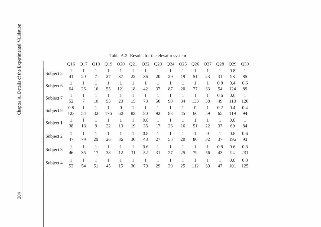
20
4C
hap
ter
A.D
etai
lso
fth
eE
xper
imen
talV
alid
atio
n
Table A.2: Results for the elevator system
Q16 Q17 Q18 Q19 Q20 Q21 Q22 Q23 Q24 Q25 Q26 Q27 Q28 Q29 Q30
1 1 1 1 1 1 1 1 1 1 1 1 1 0.8 1Subject 5
41 20 7 27 37 22 36 20 29 19 51 23 31 98 85
1 1 1 1 1 1 1 1 1 1 1 1 0.8 0.4 0.6Subject 6
64 26 16 55 121 18 42 37 87 20 77 33 54 124 89
1 1 1 1 1 1 1 1 1 1 1 1 0.6 0.6 1Subject 7
52 7 10 53 23 15 78 50 90 34 133 38 49 118 120
0.8 1 1 1 0 1 1 1 1 1 0 1 0.2 0.4 0.4Subject 8
123 54 32 176 60 83 80 92 83 45 60 59 65 119 94
1 1 1 1 1 1 0.8 1 1 1 1 1 1 0.8 1Subject 1
38 18 9 22 13 19 35 17 26 16 51 22 37 69 84
1 1 1 1 1 1 0.8 1 1 1 1 0 1 0.8 0.6Subject 2
47 79 29 26 36 30 48 27 55 20 80 32 37 196 93
1 1 1 1 1 1 0.6 1 1 1 1 1 0.8 0.6 0.8Subject 3
46 35 17 38 12 31 52 31 27 25 79 56 43 94 231
1 1 1 1 1 1 1 1 1 1 1 1 1 0.8 0.8Subject 4
52 54 51 45 15 30 79 29 29 25 112 39 47 101 125

A.4 Statistical Analysis 205
A.4 Statistical Analysis
TablesA.3 andA.4 contain the statistical data for each question. Only Q20 revealed a statisticallysignificant difference (with an error probability of 5%) between using the fisheye zoom andworking on a fully expanded model.
Table A.3: Statistical data for the mine drainage system
Fisheye ExpandedQuestion
Mean SD Mean SDt p
Q1 1.1194 0.3559 0.9941 0.4694 0.4201 0.6854Q2 2.0277 1.0028 1.6993 1.9672 0.2941 0.7762Q3 3.5661 1.2650 1.6861 1.3237 1.9587 0.0858Q4 2.4764 0.8246 1.8542 0.9083 0.9935 0.3495Q5 1.3353 0.9053 1.4259 1.7873 0.0895 0.9309Q6 4.3055 1.3321 3.7256 0.7691 0.7418 0.4794Q7 1.7690 0.6054 1.4468 0.8333 0.6166 0.5546Q8 1.3810 0.5271 0.7574 0.7177 1.3599 0.2109Q9 2.0346 0.9686 1.5708 0.9991 0.6567 0.5298Q10 2.1588 1.0782 3.4878 2.5246 0.9491 0.3704Q11 0.6300 0.6783 0.6176 0.5127 0.0288 0.9777Q12 1.4662 1.0363 1.4537 0.7991 0.0190 0.9853Q13 2.5402 1.5617 1.7208 0.8057 0.9148 0.3871Q14 0.8188 0.3923 1.0547 0.8319 0.5060 0.6265Q15 0.5664 0.2110 0.7321 0.3360 0.8208 0.4356

206 Chapter A. Details of the Experimental Validation
Table A.4: Statistical data for the elevator system
Fisheye ExpandedQuestion
Mean SD Mean SDt p
Q16 1.6437 0.7536 2.2140 0.2989 1.3660 0.2091Q17 6.2459 5.5153 2.8825 1.8992 1.1263 0.2927Q18 8.4151 4.8183 5.6006 4.0135 0.8811 0.4040Q19 1.9942 1.2907 3.3113 1.0735 1.5172 0.1677Q20 1.9692 1.9476 6.3675 2.4896 2.5948 0.0319Q21 4.4931 2.3571 3.7889 0.9841 0.5440 0.6013Q22 1.9226 0.7754 1.6891 0.4313 0.5194 0.6175Q23 2.6974 1.6715 4.0650 1.2271 1.2835 0.2353Q24 1.7284 1.1472 3.2040 0.9384 1.9028 0.0936Q25 3.8566 1.5049 4.8125 1.0680 1.0142 0.3402Q26 1.0028 0.8314 1.3423 0.4467 0.7082 0.4989Q27 2.9261 1.1007 2.2238 1.8835 0.6345 0.5435Q28 1.5598 1.2195 2.3483 0.4234 1.1913 0.2677Q29 0.4958 0.2297 0.7494 0.3155 1.2649 0.2415Q30 0.7773 0.3145 0.7054 0.3522 0.3010 0.7711

BIBLIOGRAPHY 207
Bibliography
Appert, C. and Fekete, J.-D. (2006). OrthoZoom Scroller: 1DMulti-Scale Navigation. InPro-ceedings of the SIGCHI Conference on Human Factors in Computing Systems, pages 21–30.
Bartram, L., Ho, A., Dill, J., and Henigman, F. (1995). The Continuous Zoom: A ConstrainedFisheye Technique for Viewing and Navigating Large Information Spaces. InProceedingsof the 8th Annual ACM Symposium on User Interface and Software Technology (UIST ’95),pages 207–215.
Battista, G. D., Eades, P., Tamassia, R., and Tollis, I. (1994). Annotated Bibliography on GraphDrawing Algorithms.Computational Geometry: Theory and Applications, 4:235–282.
Baudisch, P., Lee, B., and Hanna, L. (2004). Fishnet, A Fisheye Web Browser with Search TermPopouts: A Comparative Evaluation with Overview and LinearView. In Proceedings of theWorking Conference on Advanced Visual Interfaces, pages 133–140.
Bederson, B. B. (2000). Fisheye Menus. InProceedings of the 13th Annual ACM Symposium onUser Interface Software and Technology.
Bederson, B. B. and Boltman, A. (1999). Does Animation Help Users Build Mental Maps ofSpatial Information? InProceedings of the 1999 IEEE Symposium on Information Visualiza-tion (InfoVis’99), pages 28–35.
Bederson, B. B., Clamage, A., Czerwinski, M. P., and Robertson, G. G. (2004a). DateLens: AFisheye Calendar Interface for PDAs.ACM Transactions on Computer-Human Interaction,11(1):90–119.
Bederson, B. B., Grosjean, J., and Meyer, J. (2004b). Toolkit Design for Interactive StructuredGraphics.IEEE Transactions on Software Engineering, 30(8):535–546.

208 BIBLIOGRAPHY
Bederson, B. B. and Hollan, J. D. (1994). Pad++: A Zooming Graphical Interface for Explor-ing Alternate Interface Physics. InProceedings of the 7th Annual ACM Symposium on UserInterface Software and Technology, pages 17–26.
Bederson, B. B., Meyer, J., and Good, L. (2000). Jazz: An Extensible Zoomable User Inter-face Graphics Toolkit in Java. InProceedings of the 13th Annual ACM Symposium on UserInterface Software and Technology, pages 171–180.
Berner, S. (2002).Modellvisualisierung für die Spezifikationssprache ADORA. PhD thesis,Universität Zürich.
Berner, S., Joos, S., Glinz, M., and Arnold, M. (1998). A Visualization Concept for HierarchicalObject Models. InProceedings of the 13th IEEE International Conference on AutomatedSoftware Engineering (ASE’98), pages 225–228.
Booth, T. (1967).Sequential Machines and Automata Theory. John Wiley and Sons, New York.
Bourgeois, F. and Guiard, Y. (2002). Multiscale Pointing: Facilitating Pan-Zoom Coordination.In Proceedings of the ACM Conference on Human Factors in Computing Systems (CHI’02),pages 758–759.
Bridgeman, S. and Tamassia, R. (2000). Difference Metrics for Interactive Orthogonal GraphDrawing Algorithms.Journal of Graph Algorithms and Applications, 4(3):47–74.
Brooks, F. P. (1987). No Silver Bullet - Essence and Accidents of Software Engineering.IEEEComputer, 20(4):10–19.
Brooks, F. P. (1995).The Mythical Man-Month: Essays on Software Engineering. Addison-Wesley, 2nd edition.
Büring, T., Gerken, J., and Reiterer, H. (2006). User Interaction with Scatterplots on SmallScreens - A Comparative Evaluation of Geometric-Semantic Zoom and Fisheye Distortion.IEEE Transactions on Visualization and Computer Graphics, 12(5):829–836.
Card, S. K., Robertson, G. G., and Mackinlay, J. D. (1991). The Information Visualizer, anInformation Workspace. InProceedings of the SIGCHI Conference on Human Factors inComputing Systems: Reaching Through Technology, pages 181–186.
Carpendale, M. S. T., Cowperthwaite, D. J., and Fracchia, F.D. (1997a). Extending DistortionViewing from 2D to 3D.IEEE Computer Graphics and Applications, 17(4):42–51.
Carpendale, M. S. T., Cowperthwaite, D. J., and Fracchia, F.D. (1997b). Making DistortionsComprehensible. InProceedings of the IEEE Symposium on Visual Languages, pages 36–45.
Chen, P. P.-S. (1976). The Entity-Relationship Model - Toward a Unified View of Data.ACMTransactions on Database Systems, 1(1):9–36.

BIBLIOGRAPHY 209
Chimera, R. (1992). Value Bars: An Information Visualization and Navigation Tool for Multi-attribute Listings. InProceedings of the SIGCHI Conference on Human Factors in ComputingSystems, pages 293–294.
Christensen, J., Marks, J., and Shieber, S. (1995). An Empirical Study of Algorithms for Point-Feature Label Placement.ACM Transactions on Graphics, 14(3):203–232.
Chui, M. and Dillon, A. (1997). Who’s Zooming Whom? Attunement to Animation in theInterface.Journal of the American Society for Information Science, 48(11):1067–1072.
Cockburn, A., Karlson, A., and Bederson, B. B. (2008). A Review of Overview+Detail, Zoom-ing, and Focus+Context Interfaces.ACM Computing Surveys, 41(1):1–31.
Cockburn, A. and Savage, J. (2003). Comparing Speed-Dependent Automatic Zooming withTraditional Scroll, Pan, and Zoom Methods. InPeople and Computers XVII: British ComputerSociety Conference on Human Computer Interaction, pages 87–102.
Coleman, M. K. and Parker, D. S. (1996). Aesthetics-based Graph Layout for Human Consump-tion. Software: Practice and Experience, 26(12):1415–1438.
Constantine, L. L. and Lockwood, L. A. D. (1999).Software for Use: A Practical Guide to theModels and Methods of Usage-Centered Design. Addison-Wesley Professional.
Czerwinski, M. and Larson, K. (1997). The New Web Browsers: They’re Cool but Are TheyUseful? InPeople and Computers XII: British Computer Society Conference on HumanComputer Interaction.
Davies, N., Cheverst, K., Mitchell, K., and Efrat, A. (2001). Using and Determining Location ina Context-Sensitive Tour Guide.IEEE Computer, 34(8):35–41.
de Berg, M., van Kreveld, M., Overmars, M., and Schwarzkopf,O. (2000). ComputationalGeometry: Algorithms and Applications. Springer, Heidelberg, second edition.
DeMarco, T. (1979).Structured Analysis and Systems Specification. Prentice-Hall, EnglewoodCliffs, N.J.
Dijkstra, E. W. (1959). A Note on Two Problems in Connexion with Graphs. NumerischeMathematik, 1:269–271.
Dijkstra, E. W. (1968). Go To Statement Considered Harmful.Communications of the ACM,11(3):147–148.
Dijkstra, E. W. (1989). The Cruelty of Really Teaching Computer Science.Communications ofthe ACM, 32(12):1389–1404.
Dill, J., Bartram, L., Ho, A., and Henigman, F. (1994). A Continuously Variable Zoom forNavigating Large Hierarchical Networks. InProceedings of IEEE International Conferenceon Systems, Man and Cybernetics, pages 386–390.

210 BIBLIOGRAPHY
Donelson, W. C. (1978). Spatial Management of Information.In Proceedings of the 5th AnnualConference on Computer Graphics and Interactive Techniques, pages 203 – 209.
Donoho, A. W., Donoho, D. L., and Gasko, M. (1988). MacSpin: Dynamic Graphics on aDesktop Computer.IEEE Computer Graphics & Applications, 8(4):51–58.
Donskoy, M. and Kaptelinin, V. (1997). Window Navigation With and Without Animation: AComparison of Scroll Bars, Zoom, and Fisheye View. InProceedings of the Conference onHuman Factors in Computing Systems, pages 279–280.
Dori, D. (2002). Why Significant UML Change Is Unlikely.Communications of the ACM,45(11):82–85.
Eades, P. (1984). A Heuristic for Graph Drawing.Congressus Numerantium, 42:149–160.
Eades, P., Lai, W., Misue, K., and Sugiyama, K. (1991). Preserving the Mental Map of a Dia-gram. InProceedings of COMPUGRAPHICS ’91, pages 34–43.
Farrand, W. A. (1973).Information Display in Interactive Design. PhD thesis, Department ofEngineering, University of California, Los Angeles.
Filman, R. E. and Friedman, D. P. (1984).Coordinated Computing: Tools and Techniques forDistributed Software. McGraw Hill Higher Education.
Fish, A. and Störrle, H. (2007). Visual qualities of the Unified Modeling Language: Deficienciesand Improvements. InProceedings of the IEEE Symposium on Visual Languages and Human-Centric Computing, pages 41–49.
Freire, M. and Rodríguez, P. (2006). Preserving The Mental Map in Interactive Graph Interfaces.In Proceedings of the Working Conference on Advanced Visual Interfaces, pages 270–273.
Furnas, G. W. (1981). The Fisheye View: A New Look at Structured Files. Technical report,Bell Labs.
Furnas, G. W. (1986). Generalized Fisheye Views. InProceedings of the SIGCHI Conference onHuman Factors in Computing Systems, pages 16–23.
Furnas, G. W. (2006). A Fisheye Follow-up: Further Reflections on Focus + Context. InProceed-ings of the SIGCHI Conference on Human Factors in Computing Systems, pages 999–1008.
Furnas, G. W. and Bederson, B. B. (1995). Space-Scale Diagrams: Understanding Multiscale In-terfaces. InProceedings of the SIGCHI Conference on Human Factors in Computing Systems,pages 234 – 241.
Furnas, G. W. and Zhang, X. (1998). MuSE: A Multiscale Editor. In Proceedings of the 11thAnnual ACM Symposium on User Interface Software and Technology (UIST’98), pages 107–116.

BIBLIOGRAPHY 211
Gamma, E., Helm, R., Johnson, R., and Vlissides, J. (1995).Design Patterns: Elements ofReusable Object-Oriented Software. Addison-Wesley.
Gershon, N., Eick, S. G., and Card, S. (1998). Information Visualization.interactions, 5(2):9–15.
Glinz, M. (2000). Problems and Deficiencies of UML as a Requirements Specification Language.In Proceedings of the 10th International Workshop on SoftwareSpecification and Design,pages 11–22.
Glinz, M. (2002). Statecharts For Requirements Specification - As Simple As Possible, As RichAs Needed. InProceedings of the ICSE 2002 Workshop on Scenarios and StateMachines:Models, Algorithms, and Tools.
Glinz, M., Berner, S., and Joos, S. (2002). Object-orientedmodeling with ADORA.InformationSystems, 27(6):425–444.
Glinz, M., Seybold, C., and Meier, S. (2007). Simulation-Driven Creation, Validation and Evo-lution of Behavioral Requirements Models. Dagstuhl-Workshop Modellbasierte Entwicklungeingebetteter Systeme (MBEES 2007), Informatik-Bericht 2007-01, TU Braunschweig.
Goldstine, H. H. and von Neumann, J. (1947). Planning and Coding Problems for an ElectronicComputing Instrument. In Taub, A. H., editor,John von Neumann: Collected Works, volume 5,pages 80–151. McMillan, New York.
Gonzalez, C. (1996). Does Animation in User Interfaces Improve Decision Making? InPro-ceedings of the SIGCHI Conference on Human Factors in Computing Systems, pages 27–34.
Gross, J. T. and Yellen, J. (1998).Graph Theory and Its Applications. CRC Press.
Gutwin, C. (2002). Improving Focus Targeting in Interactive Fisheye Views. InProceedings ofthe SIGCHI Conference on Human Factors in Computing Systems, pages 267–274.
Gutwin, C. and Fedak, C. (2004). Interacting with Big Interfaces on Small Screens: A Compar-ison of Fisheye, Zoom, and Panning Techniques. InProceedings of Graphics Interface 2004,pages 145–152.
Harel, D. (1987). Statecharts: A Visual Formalism for Complex Systems.Science of ComputerProgramming, 8(3):231–274.
Harel, D. (1988). On Visual Formalisms.Communications of the ACM, 31(5):514–530.
Henderson, D. A. and Card, S. K. (1986). Rooms: The Use of Multiple Virtual Workspaces toReduce Space Contention in a Window-Based Graphical User Interface. ACM Transactionson Graphics, 5(3):211–243.
Herman, I., Melançon, G., and Marshall, M. S. (2000). Graph Visualization and Navigationin Information Visualization: A Survey.IEEE Transactions on Visualization and ComputerGraphics, 6(1):24–43.

212 BIBLIOGRAPHY
Herot, C. F. (1980). Spatial Management of Data.ACM Transactions on Database Systems,5(4):493–513.
Hornbæk, K., Bederson, B. B., and Plaisant, C. (2002). Navigation Patterns and Usability ofZoomable User Interfaces with and without an Overview.ACM Transactions on Computer-Human Interaction, 9(4):362–389.
Hornbæk, K. and Frøkjær, E. (2003). Reading Patterns and Usability in Visualizations of Elec-tronic Documents.ACM Transactions on Computer-Human Interaction, 10(2):119–149.
Hornbæk, K. and Hertzum, M. (2007). Untangling the Usability of Fisheye Menus.ACM Trans-actions on Computer-Human Interaction, 14(2).
Huotari, J., Lyytinen, K., and Niemelä, M. (2004). Improving Graphical Information SystemModel Use With Elision and Connecting Lines.ACM Transactions on Computer-HumanInteraction, 11(1):26–58.
IBM (1974). HIPO—A Design Aid and Documentation Technique.Technical Report GC20-1851, IBM Corporation, White Plains, NY.
IEEE (1990). Standard glossary of software engineering terminology. IEEE Std 610.12-1990.IEEE Computer Society Press.
Imhof, E. (1975). Positioning Names on Maps.The American Cartographer, 2(2):128–144.
Irani, P., Tingley, M., and Ware, C. (2001). Using Perceptual Syntax to Enhance SemanticContent in Diagrams.IEEE Computer Graphics and Applications, 21(5):76–84.
ITU-T (2000). Specification and Description Language (SDL). Recommendation Z.100(11/99),International Telecommunication Union, Geneva.
Jackson, M. A. (1975).Principles of Program Design. Academic Press.
Jakobsen, M. R. and Hornbæk, K. (2006). Evaluating a FisheyeView of Source Code. InProceedings of the SIGCHI Conference on Human Factors in Computing Systems, pages 377–386.
Joos, S. (1999). Adora-L - Eine Modellierungssprache zur Spezifikation von Software-Anforderungen. PhD thesis, University of Zurich.
Jul, S. and Furnas, G. W. (1998). Critical Zones in Desert Fog: Aids to Multiscale Navigation. InProceedings of the 11th Annual ACM Symposium on User Interface Software and Technology,pages 97–106.
Kadmon, N. and Shlomi, E. (1978). A Polyfocal Projection forStatistical Surfaces.Cartography,15(1):36–41.

BIBLIOGRAPHY 213
Kakoulis, K. G. and Tollis, I. G. (1997). An Algorithm for Labeling Edges of HierarchicalDrawings. InProceedings of the 5th International Symposium on Graph Drawing, pages169–180.
Kersten, M. and Murphy, G. C. (2005). Mylar: A Degree-of-Interest Model for IDEs. InPro-ceedings of the 4th International Conference on Aspect-Oriented Software Development, pages159–168.
Kim, J., Hahn, J., and Hahn, H. (2000). How Do We Understand a System with (So) ManyDiagrams? Cognitive Integration Processes in Diagrammatic Reasoning.Information SystemsResearch, 11(3):284–303.
Klein, C. and Bederson, B. B. (2005). Benefits of Animated Scrolling. In Proceedings of theACM Conference on Human Factors in Computing Systems (CHI’05), pages 1965–1968.
Knuth, D. (1997).The Art of Computer Programming, volume 1. Addison-Wesley, 3. edition.
Kobryn, C. (2004). Uml 3.0 and the future of modeling.Software and Systems Modeling,13(1):4–8.
Koffka, K. (1935).Principles of Gestalt Psychology. Harcourt-Brace, New York.
Kramer, J., Magee, J., Sloman, M., and Lister, A. (1983). CONIC: an integrated approach todistributed computer control systems.IEE Proceedings-E Computers and Digital Techniques,130(1):1–10.
Kruchten, P. (1995). The 4+1 View Model of Architecture.IEEE Software, 12(6):42–50.
Lamping, J., Rao, R., and Pirolli, P. (1995). A Focus+Context Technique Based on HyperbolicGeometry for Visualizing Large Hierarchies. InProceedings of the ACM Conference on Hu-man Factors in Computing Systems (CHI’95), pages 401–408.
Lee, C. Y. (1961). An Algorithm for Path Connections and its Applications. IRE Transactionson Electronic Computers, EC-10:346–365.
Leung, Y. K. and Apperley, M. D. (1994). A Review and Taxonomyof Distortion-OrientedPresentation Techniques.ACM Transactions on Computer-Human Interaction, 1(2):126 –160.
Leveson, N. G., Heimdahl, M. P. E., Hildreth, H., and Reese, J. D. (1994). Requirements Specifi-cation for Process-Control Systems.IEEE Transactions on Software Engineering, 20(9):684–707.
Li, W., Eades, P., and Hong, S.-H. (2005). Navigating Software Architectures with ConstantVisual Complexity. InProceedings of the 2005 IEEE Symposium on Visual Languages andHuman-Centric Computing (VL/HCC’05), pages 225 – 232.

214 BIBLIOGRAPHY
Ludewig, J. (2003). Models in Software Engineering - An Introduction. Software and SystemsModeling, 2(1):5–14.
Lyons, K. A., Meijer, H., and Rappaport, D. (1998). Algorithms for Cluster Busting in AnchoredGraph Drawing.Journal of Graph Algorithms and Applications, 2(1):1–24.
Mackinlay, J. D., Robertson, G. G., and Card, S. K. (1991). The Perspective Wall: Detail andContext Smoothly Integrated . InProceedings of the SIGCHI Conference on Human Factorsin Computing Systems, pages 173–176.
Marple, D., Smulders, M., and Hegen, H. (1990). Tailor: A Layout System Based on TrapezoidalCorner Stitching.IEEE Transactions on Computer-Aided Design of Integrated Circuits andSystems, 9(1):66–90.
Marty, M. (2002). Analyse und Erweiterung von Algorithmen zur logischen Navigation inADORA-Modellen. Master’s thesis, Universität Zürich.
Meier, S. (2009).Aspect-Oriented Requirements Modeling. PhD thesis, Universität Zürich.
Meier, S., Reinhard, T., Seybold, C., and Glinz, M. (2006). Aspect-Oriented Modeling withIntegrated Object Models. InModellierung 2006, volume P-82 ofGI-Edition-Lecture Notesin Informatics, pages 129–144.
Miller, G. A. (1956). The Magical Number Seven, Plus or MinusTwo: Some Limits on ourCapacity for Processing Information.Psychological Review, 63(2):81–97.
Miriyala, K., Hornick, S. W., and Tamassia, R. (1993). An Incremental Approach to AestheticGraph Layout. InProceeding of the Sixth International Workshop on Computer-Aided Soft-ware Engineering, pages 297–308.
Misue, K., Eades, P., Lai, W., and Sugiyama, K. (1995). Layout Adjustment and the MentalMap. Journal of Visual Languages and Computing, 6(2):183–210.
Moody, D. (2006). Dealing with "Map Shock": A Systematic Approach for Managing Complex-ity in Requirements Modelling. InProceedings of the 12th Working Conference on Require-ments Engineering: Foundation for Software Quality (REFSQ2006).
Moody, D. L. (2009). The "Physics" of Notations: Toward a Scientific Basis for Construct-ing Visual Notations in Software Engineering.IEEE Transactions on Software Engineering,35(6):756–779.
Mullet, K., Fry, C., and Schiano, D. (1997). On Your Marks, Get Set, Browse! InExtendedAbstracts of the ACM Conference on Human Factors in Computing Systems, pages 113–114.
Nassi, I. and Shneiderman, B. (1973). Flowchart Techniquesfor Structured Programming.ACMSIGPLAN Notices, 8(8):12–26.
BIBLIOGRAPHY 215
Nekrasovski, D., Bodnar, A., McGrenere, J., Guimbretière,F., and Munzner, T. (2006). AnEvaluation of Pan & Zoom and Rubber Sheet Navigation with andwithout an Overview. InProceedings of the SIGCHI Conference on Human Factors in Computing Systems, pages 11–20.
Noik, E. G. (1994). A Space of Presentation Emphasis Techniques for Visualizing Graphs. InProceedings of Graphics Interface ’94, pages 225–234.
Nordbotten, J. C. and Crosby, M. E. (1999). The Effect of Graphic Style on Data Model Inter-pretation.Information Systems Journal, 9(2):139–155.
North, S. C. (1996). Incremental Layout in DynaDAG. InProceedings of the 4th Symposium onGraph Drawing, pages 409–418.
OMG (2003). MDA Guide Version 1.0.1. omg/03-06-01, Object Management Group.
OMG (2005). Unified Modeling Language: Superstructure Version 2.0. Document formal/05-07-04, Object Management Group.
Ousterhout, J. K. (1984). Corner Stitching: A Data-Structuring Technique for VLSI LayoutTools. IEEE Transactions on Computer-Aided Design of Integrated Circuits and Systems,3(1):87–100.
Parnas, D. L. (1972). On the Criteria to be Used in Decomposing Systems into Modules.Com-munications of the ACM, 15(12):1053–1058.
Peleg, M. and Dori, D. (2000). The Model Multiplicity Problem: Experimenting with Real-TimeSpecification Methods.IEEE Transactions on Software Engineering, 26(8):742–759.
Perlin, K. and Fox, D. (1993). Pad: An Alternative Approach to the Computer Interface. InPro-ceedings of the 20th Annual Conference on Computer Graphicsand Interactive Techniques,pages 57 – 64.
Petre, M. (1995). Why Looking Isn’t Always Seeing: Readership Skills and Graphical Program-ming. Communications of the ACM, 38(6):33–44.
Petri, C. (1962).Kommunikation mit Automaten. PhD thesis, Technische Universität Darmstadt.
Pietriga, E. (2005). A Toolkit for Addressing HCI Issues in Visual Language Environments. InProceedings of the 2005 IEEE Symposium on Visual Languages and Human-Centric Comput-ing (VL/HCC’05), pages 145–152.
Pietriga, E., Appert, C., and Beaudouin-Lafon, M. (2007). Pointing and Beyond: An Oper-ationalization and Preliminary Evaluation of Multi-scaleSearching. InProceedings of theSIGCHI Conference on Human Factors in Computing Systems, pages 1215–1224.

216 BIBLIOGRAPHY
Pirolli, P., Card, S. K., and Wege, M. M. V. D. (2001). Visual Information Foraging in a Fo-cus+Context Visualization. InProceedings of the SIGCHI Conference on Human Factors inComputing Systems, pages 506–513.
Pirolli, P., Card, S. K., and Wege, M. M. V. D. (2003). The Effects of Information Scent on VisualSearch in the Hyperbolic Tree Browser.ACM Transactions on Computer-Human Interaction,10(1):20–53.
Plaisant, C., Grosjean, J., and Bederson, B. B. (2002). SpaceTree: Supporting Exploration inLarge Node Link Tree, Design Evolution and Empirical Evaluation. In Proceedings of theIEEE Symposium on Information Visualization (InfoVis 2002), pages 57–64.
Purchase, H. C., Carrington, D., and Allder, J.-A. (2002). Empirical Evaluation of Aesthetics-based Graph Layout.Empirical Software Engineering, 7(3):233–255.
Rao, R. and Card, S. K. (1994). The Table Lens: Merging Graphical and Symbolic Representa-tions in an Interactive Focus+Context Visualization for Tabular Information. InProceedingsof the SIGCHI Conference on Human Factors in Computing Systems, pages 318–322.
Reinhard, T. (2004). Halbautomatische Linienführung in Adora-Modellen unter Berücksichti-gung des Zoom-Algorithmus. Master’s thesis, Universität Zürich.
Reinhard, T. and Glinz, M. (2010). Automatic Placement of Link Labels in Diagrams. InICSE2010 Workshop on Flexible Modeling Tools (FlexiTools 2010).
Reinhard, T., Meier, S., and Glinz, M. (2007). An Improved Fisheye Zoom Algorithm for Visual-izing and Editing Hierarchical Models. InProceedings of the Second International Workshopon Requirements Engineering Visualization (REV’07).
Reinhard, T., Meier, S., Stoiber, R., Cramer, C., and Glinz,M. (2008). Tool Support for theNavigation in Graphical Models. InProceedings of the 30th International Conference onSoftware Engineering (ICSE’08), pages 823–826.
Reinhard, T., Seybold, C., Meier, S., Glinz, M., and Merlo-Schett, N. (2006). Human-FriendlyLine Routing for Hierarchical Diagrams. InProceedings of the 21st IEEE International Con-ference on Automated Software Engineering (ASE’06), pages 273–276.
Riel, A. J. (1996).Object-Oriented Design Heuristics. Addison-Wesley.
Robertson, G. G. and Mackinlay, J. D. (1993). The Document Lens. InProceedings of the ACMSymposium on User Interface Software and Technology, pages 101–108.
Robertson, G. G., Mackinlay, J. D., and Card, S. K. (1991). Cone Trees: Animated 3D Visu-alizations of Hierarchical Information. InProceedings of the SIGCHI Conference on HumanFactors in Computing Systems, pages 189–194.

BIBLIOGRAPHY 217
Ross, D. T. and Schoman, K. E. (1977). Structured Analysis for Requirements Definition.IEEETransactions on Software Engineering, 3(1):6–15.
Sarkar, M. and Brown, M. H. (1992). Graphical Fisheye Views of Graphs. InProceedings of theConference on Human Factors in Computing Systems, pages 83–91.
Sarkar, M., Snibbe, S. S., Tversky, O. J., and Reiss, S. P. (1993). Stretching the Rubber Sheet: AMetaphor for Viewing Large Layouts on Small Screens. InACM Symposium on User InterfaceSoftware and Technology, pages 81–91.
Scaife, M. and Rogers, Y. (1996). External Cognition: How DoGraphical RepresentationsWork? International Journal of Human-Computer Studies, 45(2):185–213.
Schaffer, D., Zuo, Z., Bartram, L., Dill, J., Dubs, S., Greenberg, S., and Roseman, M. (1993).Comparing Fisheye and Full-Zoom Techniques for Navigationof Hierarchically ClusteredNetworks. InProceedings of Graphics Interface (GI ’93).
Schaffer, D., Zuo, Z., Greenberg, S., Bartram, L., Dill, J.,Dubs, S., and Roseman, M. (1996).Navigating Hierarchically Clustered Networks through Fisheye and Full-Zoom Methods.ACM Transactions on Computer-Human Interaction, 3(2):162–188.
Schmidt, D. C. (2006). Model-Driven Engineering.IEEE Computer, 39(2):25–31.
Seybold, C. (2006). Simulation teilformaler Anforderungsmodelle. PhD thesis, UniversitätZürich.
Seybold, C., Glinz, M., Meier, S., and Merlo-Schett, N. (2003). An Effective Layout AdaptationTechnique for a Graphical Modeling Tool. InProceedings of the 25th International Conferenceon Software Engineering, pages 826 – 827.
Shneiderman, B. (1996). The Eyes Have It: A Task by Data Type Taxonomy for InformationVisualizations. InProceedings of the IEEE Symposium on Visual Languages, pages 336–343.
Shoemaker, G. and Gutwin, C. (2007). Supporting Multi-Point Interaction in Visual Workspaces.In Proceedings of the SIGCHI Conference on Human Factors in Computing Systems, pages999–1008.
Simon, H. A. (1996). The Sciences of the Artificial. The MIT Press, Cambridge, MA, thirdedition.
Sindre, G., Gulla, B., and Jokstad, H. G. (1993). Onion Graphs: Aesthetics and Layout. InProceedings of the 1993 IEEE Symposium on Visual Languages, pages 287–291.
Soukup, J. (1978). Fast Maze Router. InProceedings of the 15th conference on Design automa-tion, pages 100–102.
Spence, R. (2007).Information Visualization: Design for Interaction. Prentice Hall, secondedition.
218 BIBLIOGRAPHY
Spence, R. and Apperley, M. (1982). Data Base Navigation: AnOffice Environment for theProfessional.Behaviour & Information Technology, 1(1):43–54.
Stachowiak, H. (1973).Allgemeine Modelltheorie. Springer, Wien.
Storey, M.-A. D. and Müller, H. A. (1995). Graph Layout Adjustment Strategies. InGD ’95:Proceedings of the Symposium on Graph Drawing, pages 487–499.
Storey, M.-A. D., Wong, K., Fracchia, F. D., and Müller, H. A.(1997a). On Integrating Visual-ization Techniques for Effective Software Exploration. InProceedings of the IEEE Symposiumon Information Visualization, pages 38 – 45.
Storey, M.-A. D., Wong, K., and Müller, H. A. (1997b). How Do Program Understanding ToolsAffect How Programmers Understand Programs? InProceedings of the Fourth Working Con-ference on Reverse Engineering, pages 12–21.
Summers, K. L., Goldsmith, T. E., Kubica, S., and Caudell, T.P. (2003). An ExperimentalEvaluation of Continuous Semantic Zooming in Program Visualization. InProceedings of theIEEE Symposium on Information Visualization, pages 155–162.
Tamassia, R., di Battista, G., and Batini, C. (1988). Automatic Graph Drawing and Readabilityof Diagrams.IEEE Transactions on Systems, Man and Cybernetics, 18(1):61–79.
Tan, D. S., Robertson, G. G., and Czerwinski, M. (2001). Exploring 3D Navigation: CombiningSpeed-Coupled Flying with Orbiting. InProceedings of the SIGCHI Conference on HumanFactors in Computing Systems, pages 418–425.
Tufte, E. R. (1990).Envisioning Information. Graphics Press, Cheshire, CT.
Tufte, E. R. (1997). Visual Explanations: Images and Quantities, Evidence and Narrative.Graphics Press, Cheshire, CT.
Ware, C. (2004).Information Visualization: Perception for Design. Morgan Kaufmann, SanFrancisco, second edition.
Ware, C. and Fleet, D. (1997). Context Sensitive Flying Interface. InProceedings of the 1997Symposium on Interactive 3D Graphics, pages 127–130.
Ware, C., Hui, D., and Franck, G. (1993). Visualizing ObjectOriented Software in Three Di-mensions. InProceedings of the 1993 Conference of the Centre for Advanced Studies onCollaborative Research: Software Engineering.
Ware, C., Purchase, H., Colpoys, L., and McGill, M. (2002). Cognitive measurements of graphaesthetics.Information Visualization, 1(2):103–110.
Xia, Y. (2005). A Language Definition Method for Visual Specification Languages. PhD thesis,University of Zurich.

BIBLIOGRAPHY 219
Yoeli, P. (1972). The Logic of Automated Map Lettering.The Cartographic Journal, 9(2):99–108.
Yourdon, E. and Constantine, L. (1975).Structured Design. YOURDON Press, New York.
Zanella, A., Carpendale, M. S. T., and Rounding, M. (2002). On the Effects of Viewing Cuesin Comprehending Distortions. InProceedings of the Second Nordic Conference on Human-Computer Interaction, pages 119–128.


Curriculum Vitae
Name: Tobias Emanuel Reinhard
Date of Birth: April 27, 1980
Place of Citizenship: Horw (LU), Switzerland
1987-1992 Grammar school, Solothurn (SO)
1992-2000 High school, Solothurn (SO)
2000 Military training school
2000-2004 Studies of computer science, University of Zurich
2005-2010 Assistant and doctoral studies at the Universityof Zurich