Compressed Sensing meets

Information Theory

Dror Barondrorb@ee.technion.ac.ilwww.ee.technion.ac.il/people/drorb

Duarte

Wakin

Sarvotham

Baraniuk

Guo

Shamai

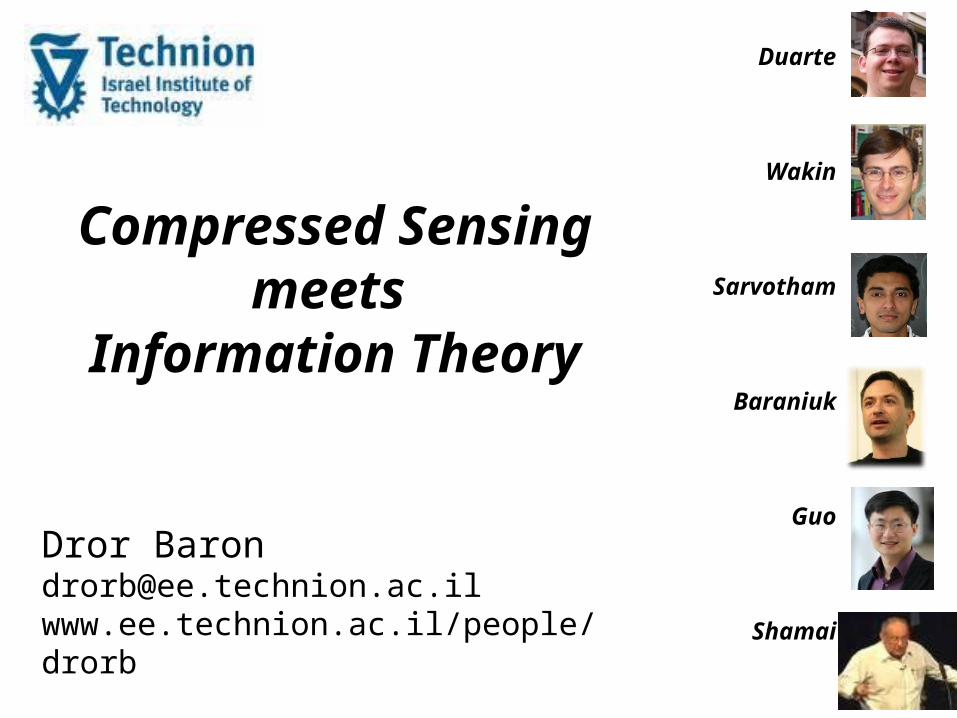
• Sensing, Computation, Communication– fast, readily available, cheap

• Progress in individual disciplines (computing, networks, comm, DSP, …)

Technology Breakthroughs

The Data Deluge

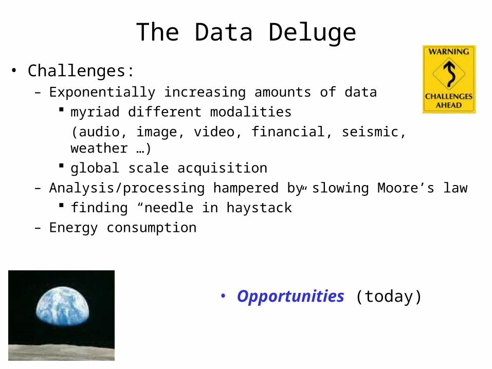
The Data Deluge• Challenges:

– Exponentially increasing amounts of data myriad different modalities

(audio, image, video, financial, seismic, weather …) global scale acquisition

– Analysis/processing hampered by slowing Moore’s law finding “needle in haystack”

– Energy consumption

• Opportunities (today)

From Sampling to Compressed Sensing

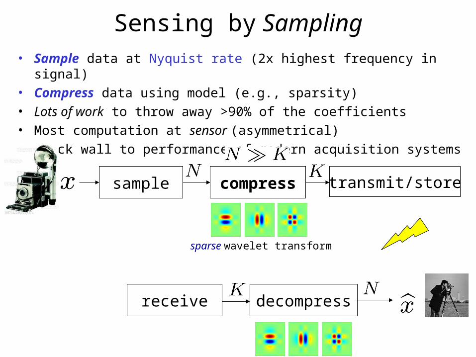
Sensing by Sampling• Sample data at Nyquist rate (2x highest frequency in signal)• Compress data using model (e.g., sparsity)• Lots of work to throw away >90% of the coefficients• Most computation at sensor (asymmetrical)• Brick wall to performance of modern acquisition systems

compress transmit/store

receive decompress

sample

sparse wavelet transform

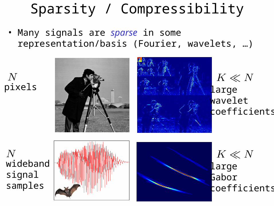
Sparsity / Compressibility

pixels largewaveletcoefficients

widebandsignalsamples

largeGaborcoefficients

• Many signals are sparse in some representation/basis (Fourier, wavelets, …)

Compressed Sensing

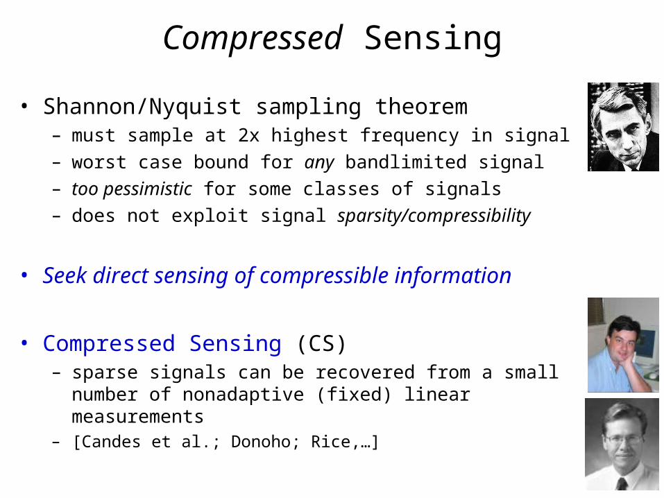
• Shannon/Nyquist sampling theorem– must sample at 2x highest frequency in signal– worst case bound for any bandlimited signal– too pessimistic for some classes of signals– does not exploit signal sparsity/compressibility

• Seek direct sensing of compressible information

• Compressed Sensing (CS)– sparse signals can be recovered from a small number

of nonadaptive (fixed) linear measurements– [Candes et al.; Donoho; Rice,…]

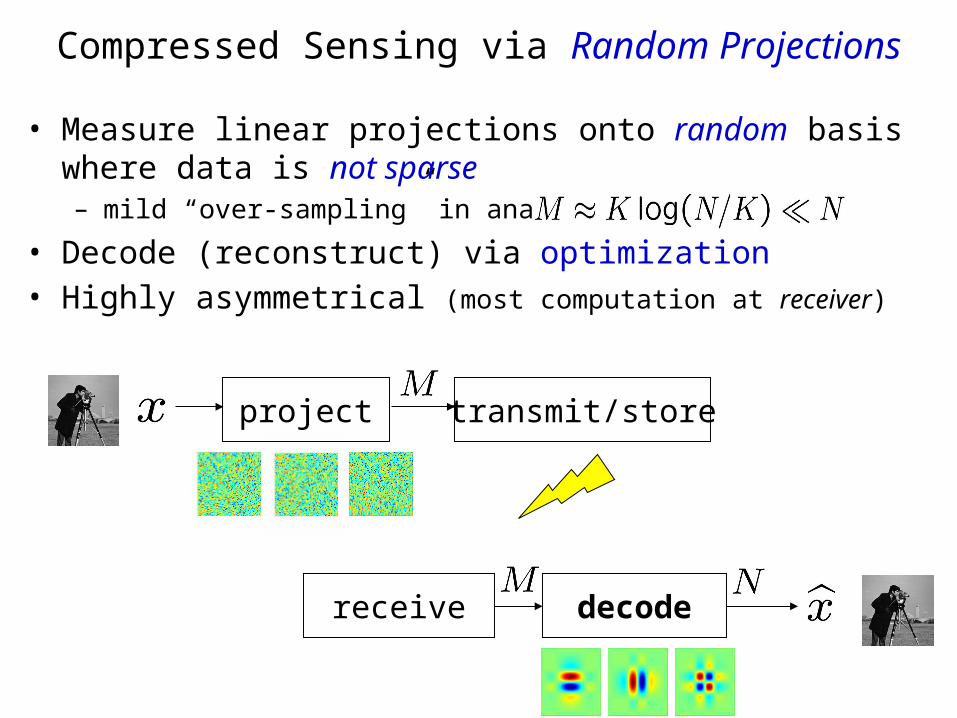
• Measure linear projections onto random basis where data is not sparse– mild “over-sampling” in analog

• Decode (reconstruct) via optimization • Highly asymmetrical (most computation at receiver)

Compressed Sensing via Random Projections

project transmit/store

receive decode

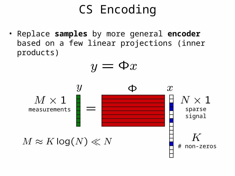
CS Encoding

• Replace samples by more general encoder based on a few linear projections (inner products)

measurements sparsesignal

# non-zeros

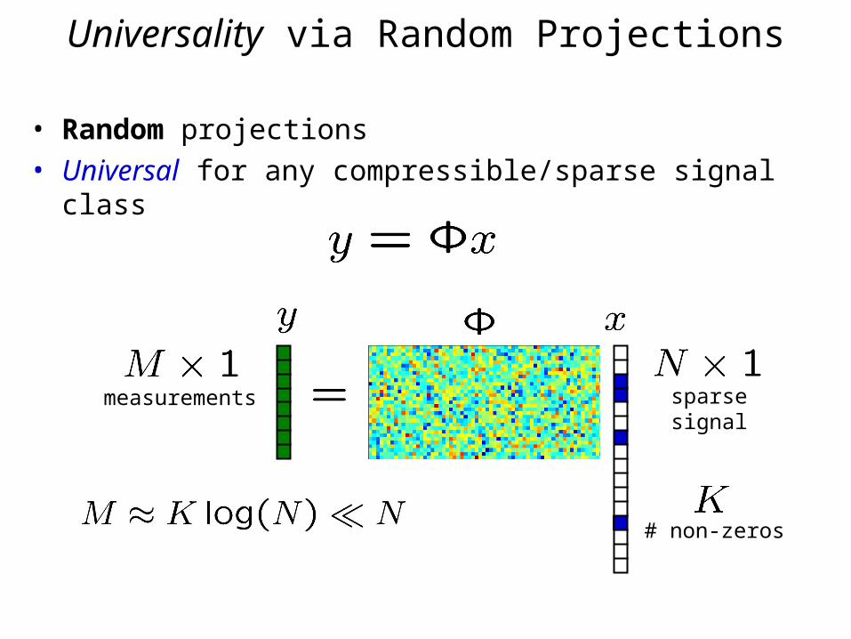
• Random projections• Universal for any compressible/sparse signal class

measurements sparsesignal

Universality via Random Projections

# non-zeros

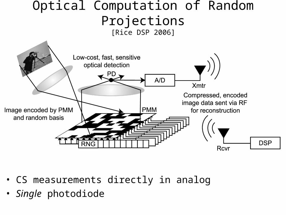
Optical Computation of Random Projections[Rice DSP 2006]

• CS measurements directly in analog• Single photodiode

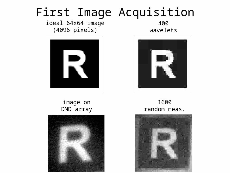
First Image Acquisitionideal 64x64 image

(4096 pixels)400

wavelets

image onDMD array

1600random meas.

• Goal: find x given y• Ill-posed inverse problem

• Decoding approach– search over subspace of explanations to measurements– find “most likely” explanation– universality accounted for during optimization

• Linear program decoding [Candes et al., Donoho] – small number of samples – computationally tractable

• Variations– greedy (matching pursuit) [Tropp et al., Needell et al.,...]

– optimization [Hale et al., Figueiredo et al.]

CS Signal Decoding

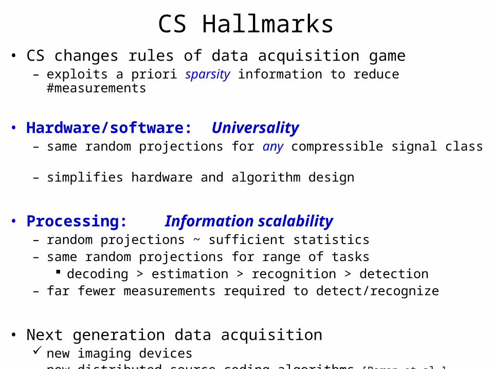
CS Hallmarks• CS changes rules of data acquisition game

– exploits a priori sparsity information to reduce #measurements

• Hardware/software: Universality– same random projections for any compressible signal class

– simplifies hardware and algorithm design

• Processing: Information scalability– random projections ~ sufficient statistics– same random projections for range of tasks

decoding > estimation > recognition > detection– far fewer measurements required to detect/recognize

• Next generation data acquisition new imaging devices– new distributed source coding algorithms [Baron et al.]

CS meets Information Theoretic Bounds[Sarvotham, Baron, & Baraniuk 2006][Guo, Baron, & Shamai 2009]

Fundamental Goal: Minimize

• Compressed sensing aims to minimize resource consumption due to measurements

• Donoho: “Why go to so much effort to acquire all the data when most of what we get will be thrown away?”

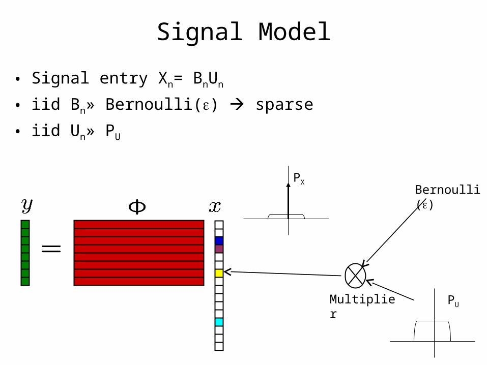
Signal Model

• Signal entry Xn= BnUn

• iid Bn» Bernoulli() sparse

• iid Un» PU

PU

Bernoulli()

Multiplier

PX

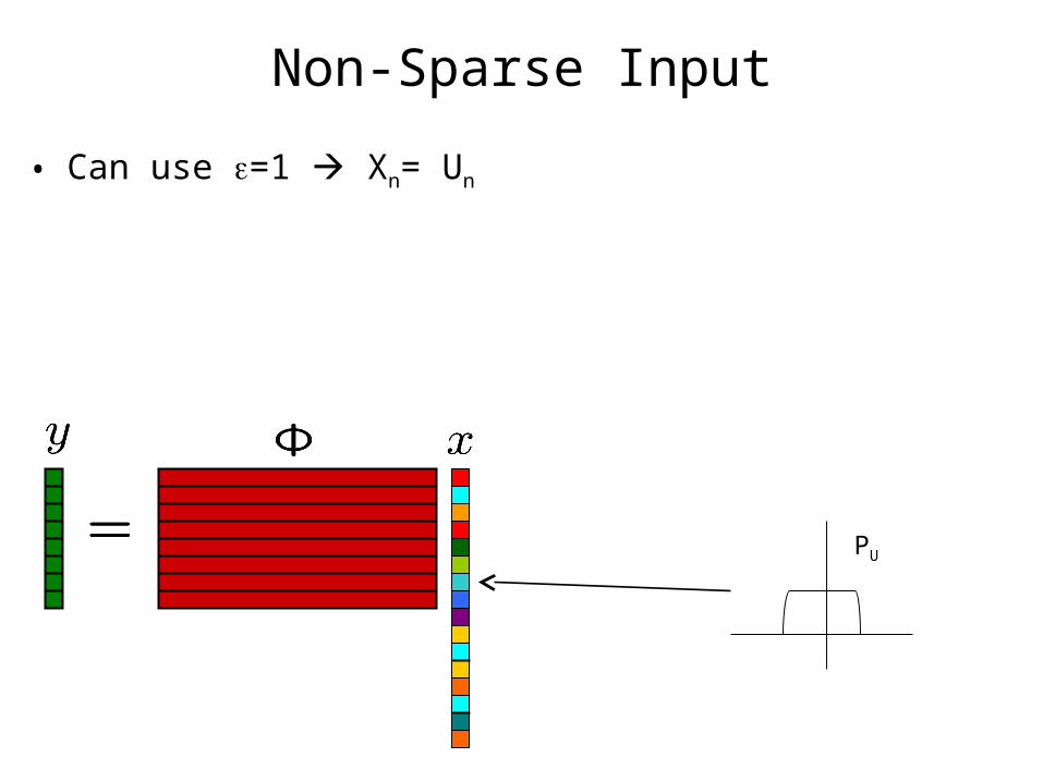
Non-Sparse Input

• Can use =1 Xn= Un

PU

Measurement Noise• Measurement process is typically analog• Analog systems add noise, non-linearities, etc.

• Assume Gaussian noise for ease of analysis

• Can be generalized to non-Gaussian noise

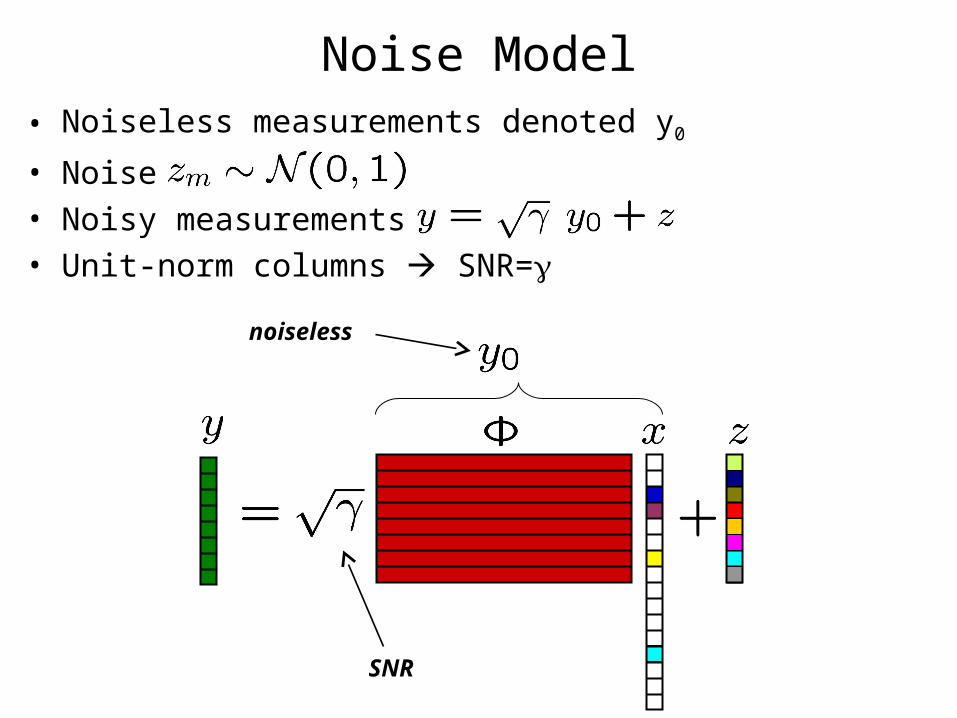
• Noiseless measurements denoted y0

• Noise• Noisy measurements• Unit-norm columns SNR=

Noise Model

noiseless

SNR

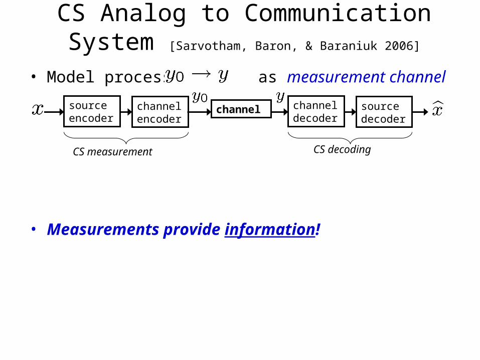
• Model process as measurement channel

• Measurements provide information!

channel

CS measurement CS decoding

source encoder

channel encoder

channel decoder

source decoder

CS Analog to Communication System [Sarvotham, Baron, & Baraniuk 2006]

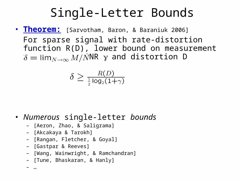
• Theorem: [Sarvotham, Baron, & Baraniuk 2006] For sparse signal with rate-distortion function R(D), lower bound on measurement rate

s.t. SNR and distortion D

• Numerous single-letter bounds – [Aeron, Zhao, & Saligrama]– [Akcakaya & Tarokh]– [Rangan, Fletcher, & Goyal]– [Gastpar & Reeves]– [Wang, Wainwright, & Ramchandran]– [Tune, Bhaskaran, & Hanly]– …

Single-Letter Bounds

Goal: Precise Single-letter Characterization of Optimal CS

[Guo, Baron, & Shamai 2009]

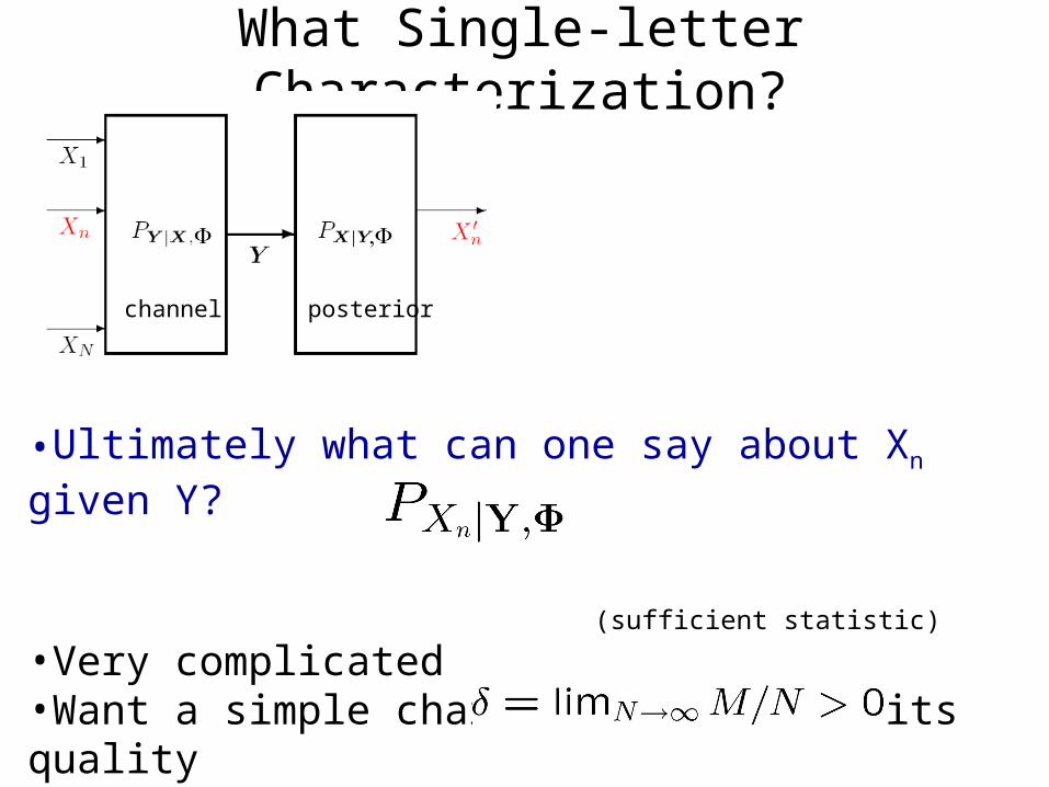
What Single-letter Characterization?

•Ultimately what can one say about Xn given Y?

(sufficient statistic)

•Very complicated•Want a simple characterization of its quality•Large-system limit:

channel posterior

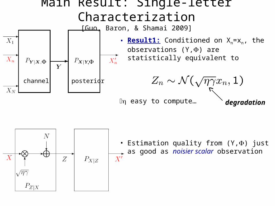
Main Result: Single-letter Characterization[Guo, Baron, & Shamai 2009]

• Result1: Conditioned on Xn=xn, the observations (Y,) are statistically equivalent to

easy to compute…

• Estimation quality from (Y,) just as good as noisier scalar observation

degradation

channel posterior

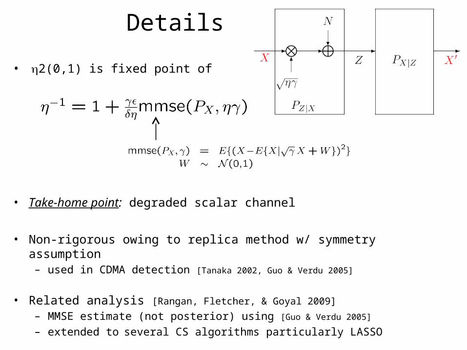
• 2(0,1) is fixed point of

• Take-home point: degraded scalar channel

• Non-rigorous owing to replica method w/ symmetry assumption– used in CDMA detection [Tanaka 2002, Guo & Verdu 2005]

• Related analysis [Rangan, Fletcher, & Goyal 2009] – MMSE estimate (not posterior) using [Guo & Verdu 2005]

– extended to several CS algorithms particularly LASSO

Details

Decoupling

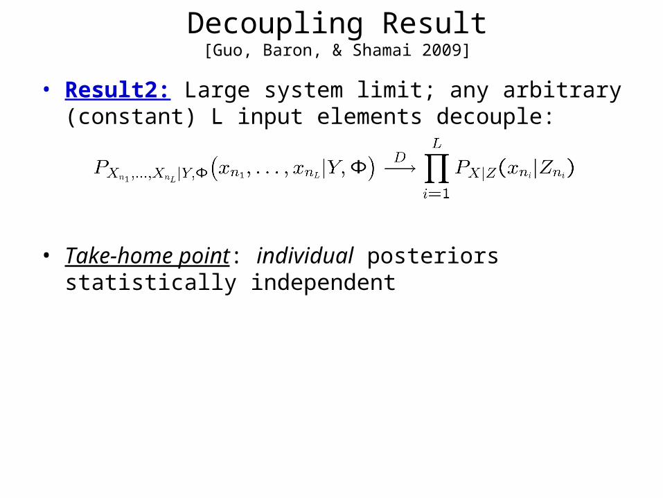
• Result2: Large system limit; any arbitrary (constant) L input elements decouple:

• Take-home point: individual posteriors statistically independent

Decoupling Result[Guo, Baron, & Shamai 2009]

Sparse Measurement Matrices

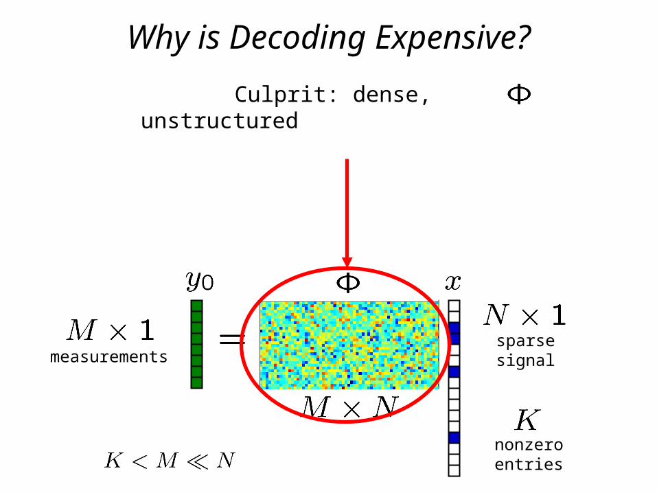
Why is Decoding Expensive?

measurementssparsesignal

nonzeroentries

Culprit: dense, unstructured

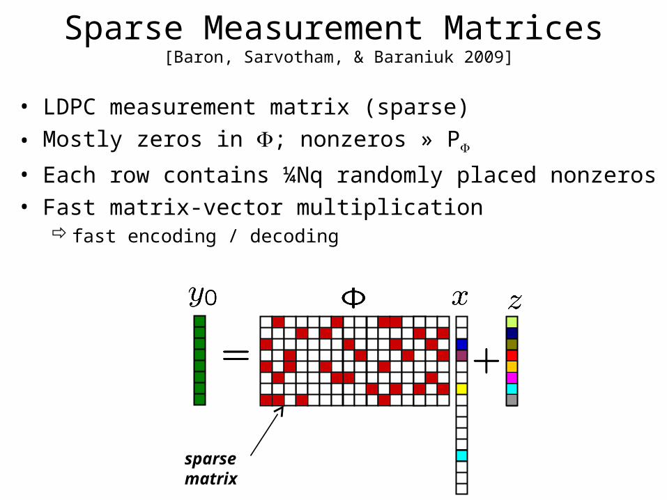
Sparse Measurement Matrices [Baron, Sarvotham, & Baraniuk 2009]

• LDPC measurement matrix (sparse)

• Mostly zeros in ; nonzeros » P

• Each row contains ¼Nq randomly placed nonzeros • Fast matrix-vector multiplication

fast encoding / decoding

sparse matrix

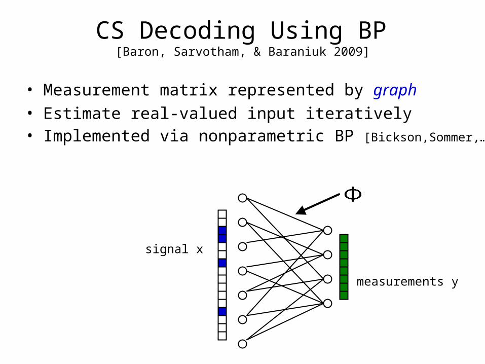
CS Decoding Using BP [Baron, Sarvotham, & Baraniuk 2009]

• Measurement matrix represented by graph • Estimate real-valued input iteratively• Implemented via nonparametric BP [Bickson,Sommer,…]

measurements y

signal x

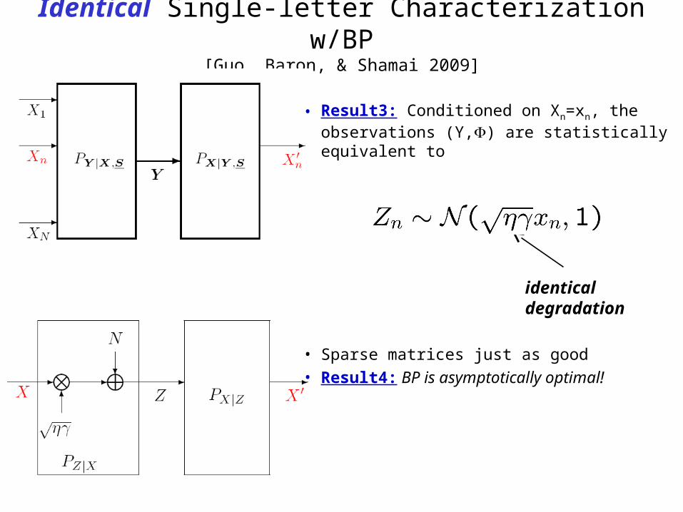
Identical Single-letter Characterization w/BP[Guo, Baron, & Shamai 2009]

• Result3: Conditioned on Xn=xn, the observations (Y,) are statistically equivalent to

• Sparse matrices just as good• Result4: BP is asymptotically optimal!

identical degradation

Decoupling Between Two Input Entries (N=500, M=250, =0.1, =10)

density

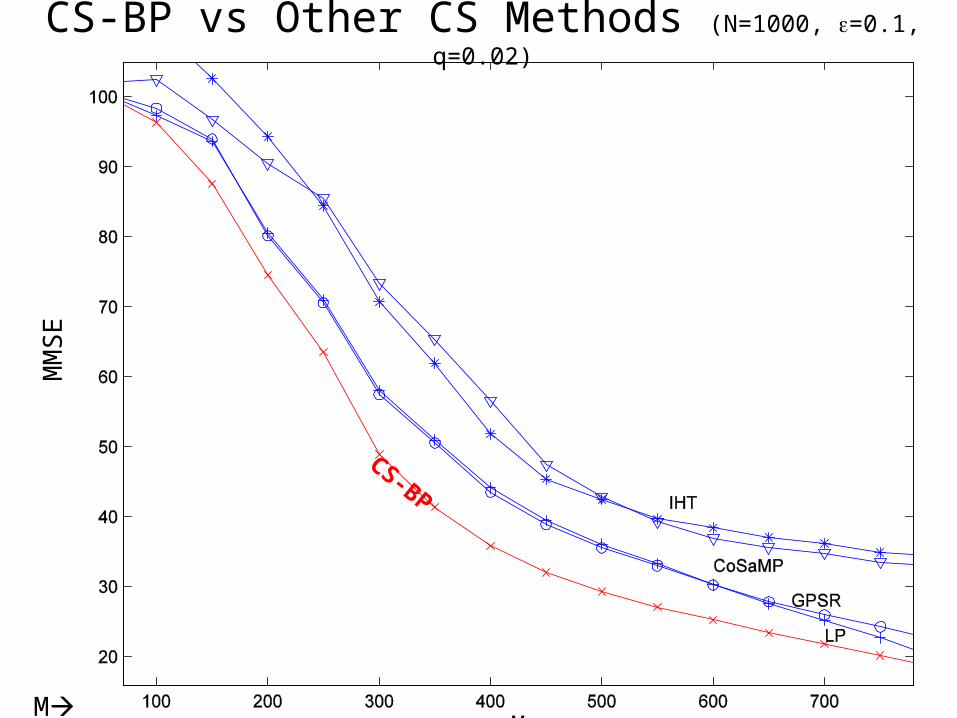
CS-BP vs Other CS Methods (N=1000, =0.1, q=0.02)

M

MM

SE

CS-BP

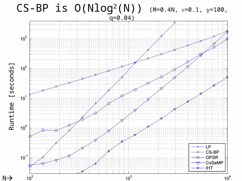
CS-BP is O(Nlog2(N)) (M=0.4N, =0.1, =100, q=0.04)R

un

tim

e [

seco

nd

s]

N

Fast CS Decoding [Sarvotham, Baron, & Baraniuk 2006]

Setting

measurementssparsesignal

nonzeroentries

• LDPC measurement matrix (sparse)• Fast matrix-vector multiplication • Assumptions:

– noiseless measurements– strictly sparse signal

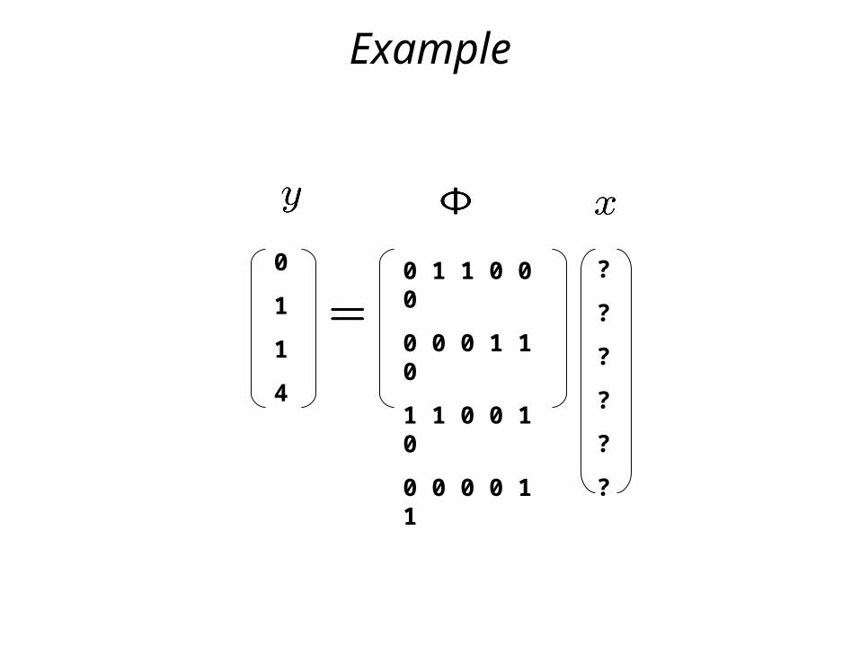
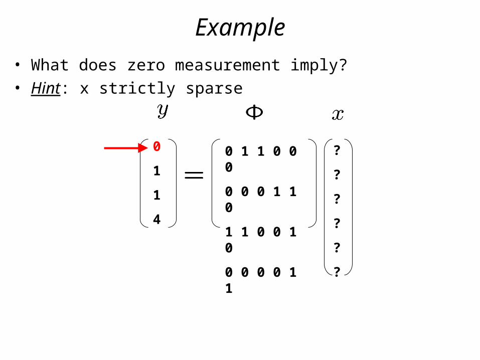
Example

0

1

1

4

0 1 1 0 0 0

0 0 0 1 1 0

1 1 0 0 1 0

0 0 0 0 1 1

?

?

?

?

?

?

Example

0

1

1

4

0 1 1 0 0 0

0 0 0 1 1 0

1 1 0 0 1 0

0 0 0 0 1 1

?

?

?

?

?

?

• What does zero measurement imply?• Hint: x strictly sparse

Example

0

1

1

4

0 1 1 0 0 0

0 0 0 1 1 0

1 1 0 0 1 0

0 0 0 0 1 1

?

0

0

?

?

?

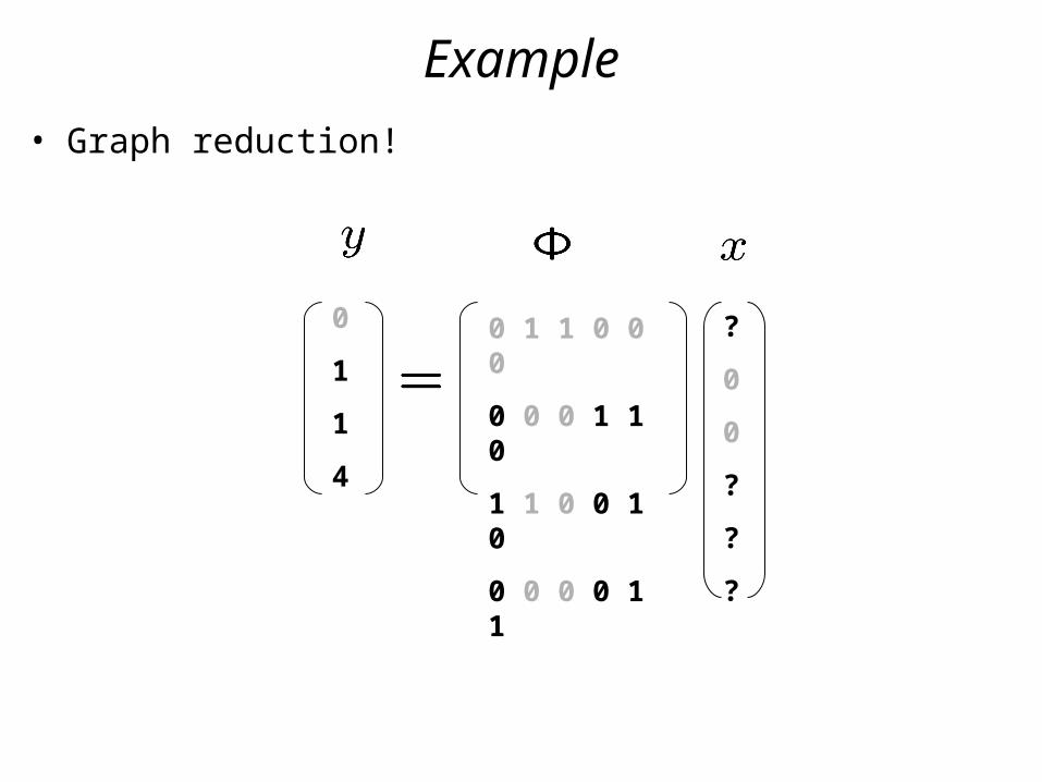
• Graph reduction!

Example

0

1

1

4

0 1 1 0 0 0

0 0 0 1 1 0

1 1 0 0 1 0

0 0 0 0 1 1

?

0

0

?

?

?

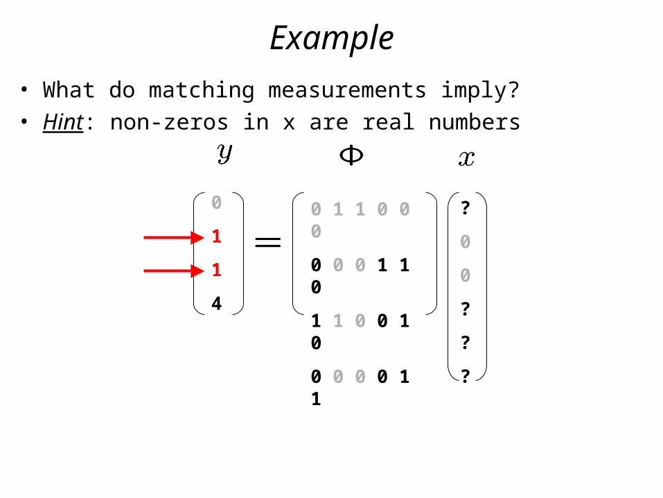
• What do matching measurements imply?• Hint: non-zeros in x are real numbers

Example

0

1

1

4

0 1 1 0 0 0

0 0 0 1 1 0

1 1 0 0 1 0

0 0 0 0 1 1

0

0

0

0

1

?

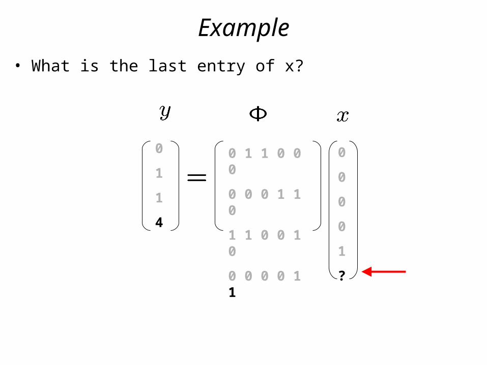
• What is the last entry of x?

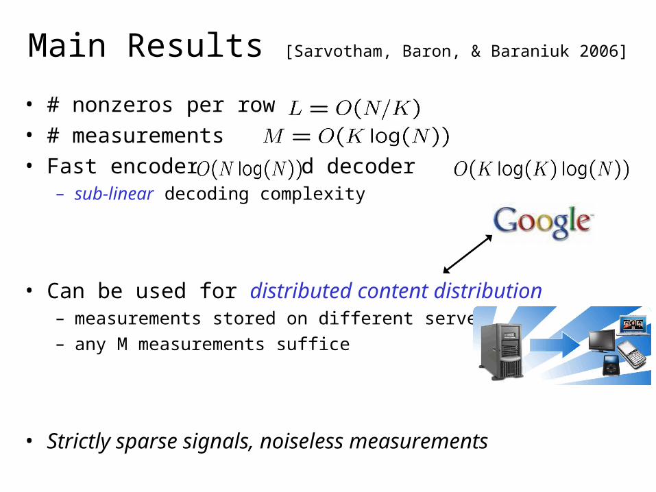
Main Results [Sarvotham, Baron, & Baraniuk 2006]

• # nonzeros per row• # measurements• Fast encoder and decoder

– sub-linear decoding complexity

• Can be used for distributed content distribution– measurements stored on different servers– any M measurements suffice

• Strictly sparse signals, noiseless measurements

Related Direction: Linear Measurements

unified theory for linear measurement systems

Linear Measurements in Finance

• Fama and French three factor model (1993)– stock returns explained by linear exposure to factors

e.g., “market” (change in stock market index)– numerous factors can be used (e.g., earnings to price)

• Noisy linear measurements

stock returns unexplained

(typically big)

exposuresfactor returns

Financial Prediction• Explanatory power ¼ prediction (can invest on this)• Goal: estimate x to explain y well

• Financial prediction vs CS: longer y, shorter x• Sounds easy, nonetheless challenging

– NOISY data need lots of measurements– nonlinear, nonstationary

compressed sensing financial prediction

Application Areas for Linear Measurements

• DSP (CS)

• Finance

• Medical imaging (tomography)

• Information retrieval

• Seismic imaging (oil industry)

Unified Theory of Linear Measurement

• Common goals– minimal resources – robustness– computationally tractable

• Inverse problems

• Striving toward theory and efficient processing in linear measurement systems

THE END