Embed Size (px)
Citation preview
Compression Displacement and Strain Estimation using
MATLAB Simulation Algorithms
Steven Sivewright
Phillip Chesnut
12/16/2008
Abstract: Advancements have been made on several fronts in improving the performance of 2-D displacement estimations between compressed and uncompressed ultrasound signals. We based our 2-D estimator work on the WaveDisp.mat function of OHS from Spring ’08. Achievements were typically made by isolating particular sections of code to determine their function, then optimizing and reinserting the code. The primary method of research for optimization was Matlab Help, especially sections on xcorr and maxlags, and the work of previous students. Operating time was greatly reduced by optimization, particularly moving the signal resampling outside of the main for loops and implementing a more efficient xcorr-mimicing function for certain conditions. In addition, output strain results were improved to accurately reflect the true strain based on newly created simulation data ‘simSC.mat’ and ‘elasticitySimImages.mat’. One of the goals we were unable to improve upon was to improve the blip-protection portion of the algorithm which accounted for the possibility of largely inaccurate displacement calculations. This was partially due to a lack of time but also because the simulation files, under several testing conditions, did not have blip problems. Overall, the function is much closer to being capable of real-world implementation. Several problems with accuracy and function inconsistencies are noted in the report to follow, as well as analysis of the new function’s capabilities with respect to inclusion size, difference in strain, and variations in system parameters. Introduction: Overview: This paper encompasses the design and testing of an algorithm produced to measure and plot displacement and strain information for one-dimensional and three-dimensional ultrasound compression information. The prior semester’s students have already researched and formed algorithms that achieve this purpose. Our goal was to evaluate and update these current algorithms to improve accuracy and reduce run time. The following report provides the results of our research and analysis.
Problem Statement: Produce an algorithm to measure and plot displacement and strain information between two ultrasound images produced at different time intervals during compression of an elastic material.

Background: Displacement and strain imaging is a valuable tool in medical research and analysis. One example of this is the detection and removal of tumors. For example, prostate carcinoma is rarely visible using conventional ultrasound means. By applying strain imaging, which involves compression of the tissue to calculate strain with respect to a set of reference data, we get a multi-dimensional representation of the tissue hardness along with the ability to detect deep lying tumors. Statistics show that only 34% of carcinoma cases were recognizable by conventional ultrasound techniques while 76% of carcinoma cases were detectable using strain imaging1. To be useful in medical applications, strain imaging software should run almost instantaneously with as little error in measurement as possible. Project Objectives: Improve an algorithm created by Spring 2008 students that was used to measure and plot two-dimensional displacement and strain information between two given ultrasound compression datasets, one of which was the signal with compression and the other being a reference signal. The goals for the code were as follows:
Increase speed by optimizing code.
Modify blip protection to accurately represent data.
Thoroughly test and analyze algorithms to determine limitations of use.
Provide clear code comments such that future students can understand our work and easily contribute their own advancements.
1 http://www.lp-it.de/download/overview-strain-imaging.pdf
Strategy: There were two distinct parts to our strategy: (1) Learn the two-dimensional function processes and create a user-friendly interface through the design of a one dimensional algorithm. (2) Experiment in an attempt to optimize the code that the previous semester’s groups (primarily OSH) had already presented. Strategy for the One‐Dimensional Algorithm: In order to better understand last semester’s two-dimensional algorithms, we produced a one-dimensional algorithm from the code contained within the current two-dimensional algorithms. The goal of this one-dimensional algorithm was to measure and plot displacement data between two given signals. Once a displacement was successfully created, we began making changes to the function that would allow more information to be given and to make the function more user-friendly. We created an input system that would allow the user to input parameters that would need to be varied on a usual basis. We also added three figures that would simultaneously plot various information throughout the function in order to better understand the functionality of the algorithm and better troubleshoot errors that may occur. One‐Dimensional Algorithm Operation: Oned3.m is an algorithm produced to measure and display displacement information for one-dimensional data. This algorithm can be seen in Appendix A. The algorithm is initialized by the user inputting the following data:
Signal 1 Signal 2 Window Size Overlap Up-Sample Factor
These input values will alter the values of maxlag and blip which will be explained in the upcoming paragraphs along with the input signals listed. The following is a step-by-step analysis of the algorithm.
1. Window sizes set by algorithm (small_low, small_high, large_low,
large_high) Two windows will be used to define an area of data within the signal to be analyzed. A large window and small window represent the two windows that will be used. These windows will be created based on the window size information given by the user.
2. Small window of data is taken from signal 1 (data1) 3. Large window of data is taken from signal 2 (data2) 4. Signal 1 and signal 2 are re-sampled in order to produce a smoother and
more effective curve of data. (redata1 & redata2) The up-sample factor given by the user determines the amount re-samples that will occur.
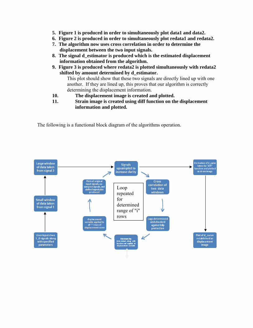
5. Figure 1 is produced in order to simultaneously plot data1 and data2. 6. Figure 2 is produced in order to simultaneously plot redata1 and redata2. 7. The algorithm now uses cross correlation in order to determine the
displacement between the two input signals. 8. The signal d_estimator is produced which is the estimated displacement
information obtained from the algorithm. 9. Figure 3 is produced where redata2 is plotted simultaneously with redata2
shifted by amount determined by d_estimator. This plot should show that these two signals are directly lined up with one another. If they are lined up, this proves that our algorithm is correctly determining the displacement information.
10. The displacement image is created and plotted. 11. Strain image is created using diff function on the displacement
information and plotted. The following is a functional block diagram of the algorithms operation.
Loop repeated for determined range of "i" rows
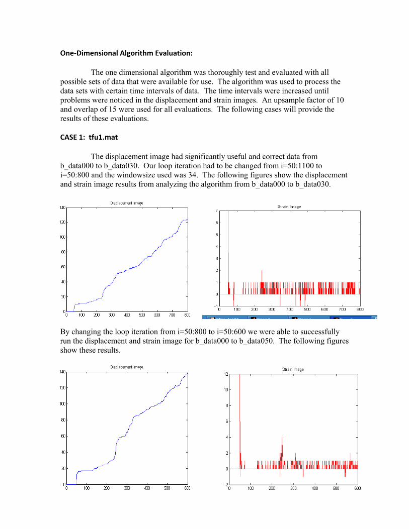
One‐Dimensional Algorithm Evaluation: The one dimensional algorithm was thoroughly test and evaluated with all possible sets of data that were available for use. The algorithm was used to process the data sets with certain time intervals of data. The time intervals were increased until problems were noticed in the displacement and strain images. An upsample factor of 10 and overlap of 15 were used for all evaluations. The following cases will provide the results of these evaluations. CASE 1: tfu1.mat The displacement image had significantly useful and correct data from b_data000 to b_data030. Our loop iteration had to be changed from i=50:1100 to i=50:800 and the windowsize used was 34. The following figures show the displacement and strain image results from analyzing the algorithm from b_data000 to b_data030.
By changing the loop iteration from i=50:800 to i=50:600 we were able to successfully run the displacement and strain image for b_data000 to b_data050. The following figures show these results.
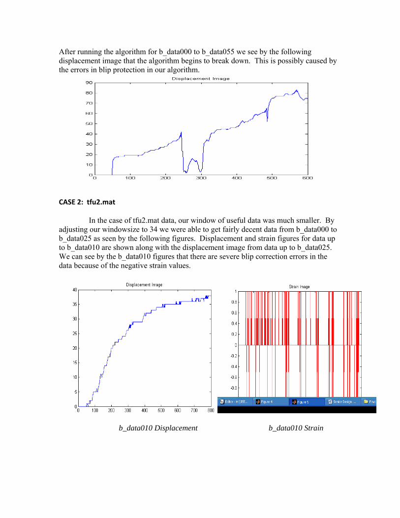
After running the algorithm for b_data000 to b_data055 we see by the following displacement image that the algorithm begins to break down. This is possibly caused by the errors in blip protection in our algorithm.
CASE 2: tfu2.mat In the case of tfu2.mat data, our window of useful data was much smaller. By adjusting our windowsize to 34 we were able to get fairly decent data from b_data000 to b_data025 as seen by the following figures. Displacement and strain figures for data up to b_data010 are shown along with the displacement image from data up to b_data025. We can see by the b_data010 figures that there are severe blip correction errors in the data because of the negative strain values.
b_data010 Displacement b_data010 Strain
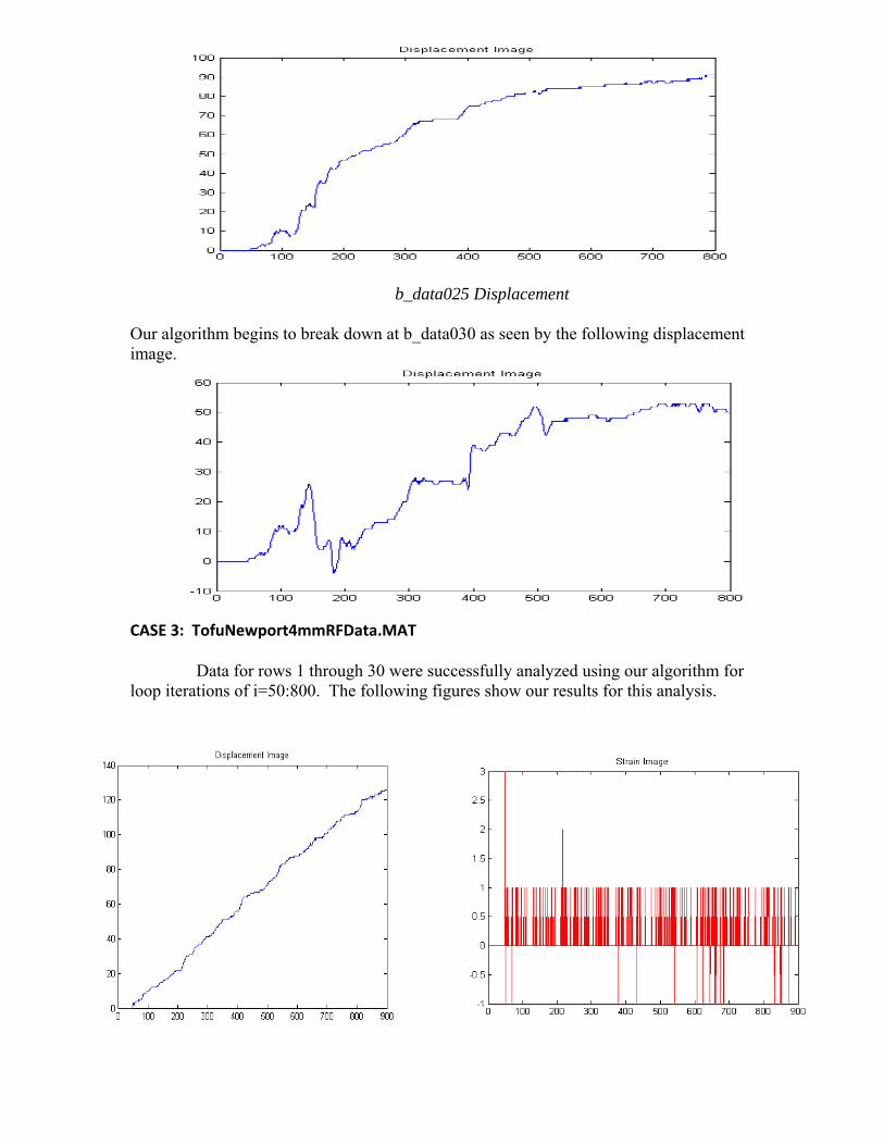
b_data025 Displacement Our algorithm begins to break down at b_data030 as seen by the following displacement image.
CASE 3: TofuNewport4mmRFData.MAT Data for rows 1 through 30 were successfully analyzed using our algorithm for loop iterations of i=50:800. The following figures show our results for this analysis.
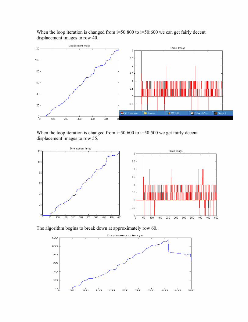
When the loop iteration is changed from i=50:800 to i=50:600 we can get fairly decent displacement images to row 40.
When the loop iteration is changed from i=50:600 to i=50:500 we get fairly decent displacement images to row 55.
The algorithm begins to break down at approximately row 60.
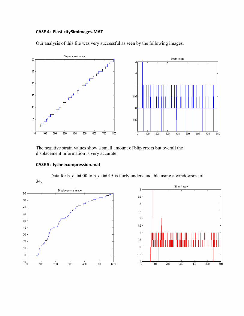
CASE 4: ElasticitySimImages.MAT Our analysis of this file was very successful as seen by the following images.
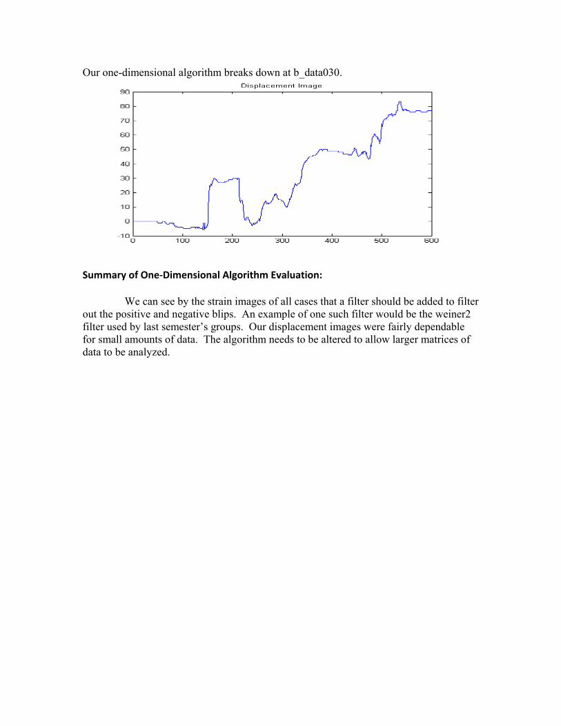
The negative strain values show a small amount of blip errors but overall the displacement information is very accurate. CASE 5: lycheecompression.mat
Data for b_data000 to b_data015 is fairly understandable using a windowsize of 34.
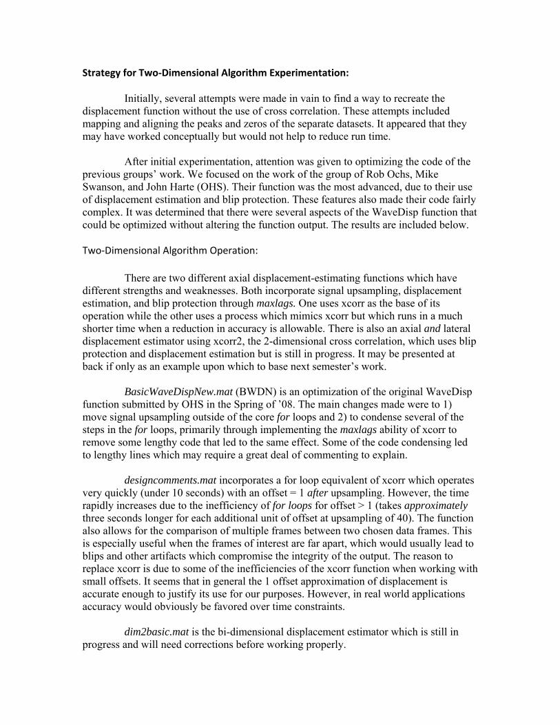
Our one-dimensional algorithm breaks down at b_data030.
Summary of One‐Dimensional Algorithm Evaluation: We can see by the strain images of all cases that a filter should be added to filter out the positive and negative blips. An example of one such filter would be the weiner2 filter used by last semester’s groups. Our displacement images were fairly dependable for small amounts of data. The algorithm needs to be altered to allow larger matrices of data to be analyzed.
Strategy for Two‐Dimensional Algorithm Experimentation: Initially, several attempts were made in vain to find a way to recreate the displacement function without the use of cross correlation. These attempts included mapping and aligning the peaks and zeros of the separate datasets. It appeared that they may have worked conceptually but would not help to reduce run time. After initial experimentation, attention was given to optimizing the code of the previous groups’ work. We focused on the work of the group of Rob Ochs, Mike Swanson, and John Harte (OHS). Their function was the most advanced, due to their use of displacement estimation and blip protection. These features also made their code fairly complex. It was determined that there were several aspects of the WaveDisp function that could be optimized without altering the function output. The results are included below. Two‐Dimensional Algorithm Operation:
There are two different axial displacement-estimating functions which have different strengths and weaknesses. Both incorporate signal upsampling, displacement estimation, and blip protection through maxlags. One uses xcorr as the base of its operation while the other uses a process which mimics xcorr but which runs in a much shorter time when a reduction in accuracy is allowable. There is also an axial and lateral displacement estimator using xcorr2, the 2-dimensional cross correlation, which uses blip protection and displacement estimation but is still in progress. It may be presented at back if only as an example upon which to base next semester’s work. BasicWaveDispNew.mat (BWDN) is an optimization of the original WaveDisp function submitted by OHS in the Spring of ’08. The main changes made were to 1) move signal upsampling outside of the core for loops and 2) to condense several of the steps in the for loops, primarily through implementing the maxlags ability of xcorr to remove some lengthy code that led to the same effect. Some of the code condensing led to lengthy lines which may require a great deal of commenting to explain. designcomments.mat incorporates a for loop equivalent of xcorr which operates very quickly (under 10 seconds) with an offset = 1 after upsampling. However, the time rapidly increases due to the inefficiency of for loops for offset > 1 (takes approximately three seconds longer for each additional unit of offset at upsampling of 40). The function also allows for the comparison of multiple frames between two chosen data frames. This is especially useful when the frames of interest are far apart, which would usually lead to blips and other artifacts which compromise the integrity of the output. The reason to replace xcorr is due to some of the inefficiencies of the xcorr function when working with small offsets. It seems that in general the 1 offset approximation of displacement is accurate enough to justify its use for our purposes. However, in real world applications accuracy would obviously be favored over time constraints. dim2basic.mat is the bi-dimensional displacement estimator which is still in progress and will need corrections before working properly.
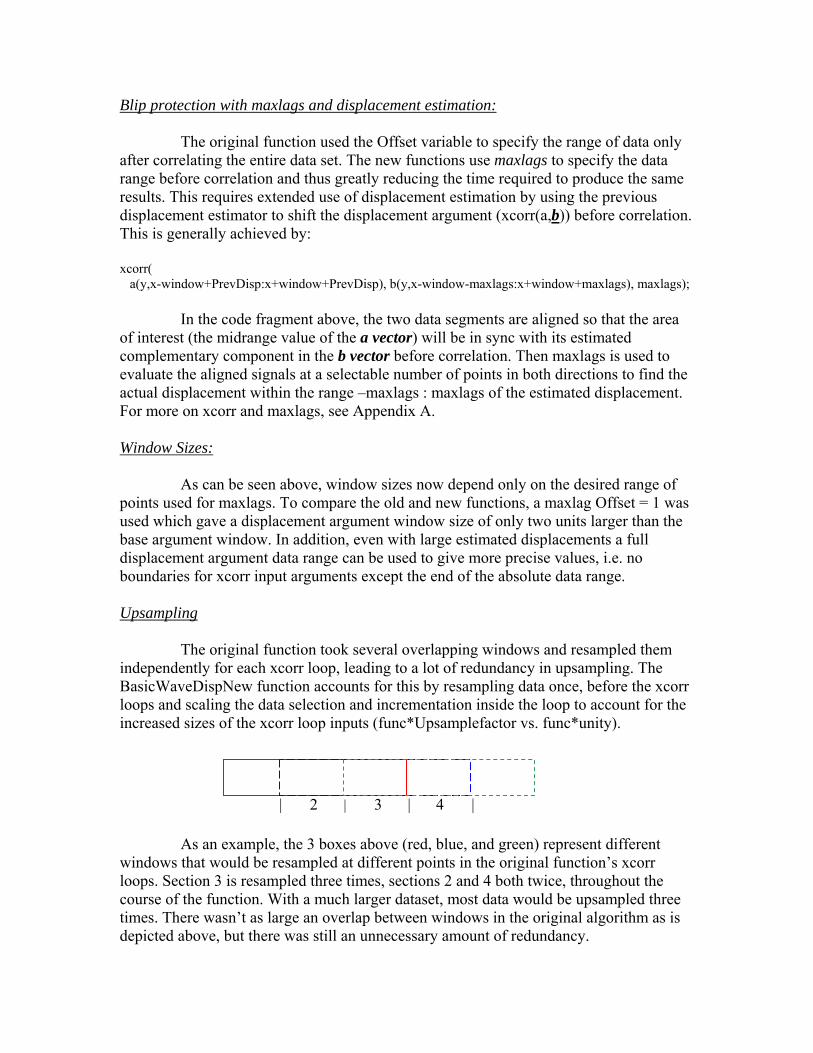
Blip protection with maxlags and displacement estimation: The original function used the Offset variable to specify the range of data only after correlating the entire data set. The new functions use maxlags to specify the data range before correlation and thus greatly reducing the time required to produce the same results. This requires extended use of displacement estimation by using the previous displacement estimator to shift the displacement argument (xcorr(a,b)) before correlation. This is generally achieved by: xcorr( a(y,x-window+PrevDisp:x+window+PrevDisp), b(y,x-window-maxlags:x+window+maxlags), maxlags); In the code fragment above, the two data segments are aligned so that the area of interest (the midrange value of the a vector) will be in sync with its estimated complementary component in the b vector before correlation. Then maxlags is used to evaluate the aligned signals at a selectable number of points in both directions to find the actual displacement within the range –maxlags : maxlags of the estimated displacement. For more on xcorr and maxlags, see Appendix A. Window Sizes: As can be seen above, window sizes now depend only on the desired range of points used for maxlags. To compare the old and new functions, a maxlag Offset = 1 was used which gave a displacement argument window size of only two units larger than the base argument window. In addition, even with large estimated displacements a full displacement argument data range can be used to give more precise values, i.e. no boundaries for xcorr input arguments except the end of the absolute data range. Upsampling The original function took several overlapping windows and resampled them independently for each xcorr loop, leading to a lot of redundancy in upsampling. The BasicWaveDispNew function accounts for this by resampling data once, before the xcorr loops and scaling the data selection and incrementation inside the loop to account for the increased sizes of the xcorr loop inputs (func*Upsamplefactor vs. func*unity). | 2 | 3 | 4 | As an example, the 3 boxes above (red, blue, and green) represent different windows that would be resampled at different points in the original function’s xcorr loops. Section 3 is resampled three times, sections 2 and 4 both twice, throughout the course of the function. With a much larger dataset, most data would be upsampled three times. There wasn’t as large an overlap between windows in the original algorithm as is depicted above, but there was still an unnecessary amount of redundancy.
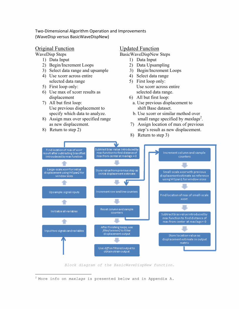
Two‐Dimensional Algorithm Operation and Improvements (WaveDisp versus BasicWaveDispNew)
Original Function Updated Function WaveDisp Steps BasicWaveDispNew Steps
1) Data Input 1) Data Input 2) Begin/Increment Loops 2) Data Upsampling 3) Select data range and upsample 3) Begin/Increment Loops 4) Use xcorr across entire 4) Select data range selected data range 5) First loop only: 5) First loop only: Use xcorr across entire 6) Use max of xcorr results as selected data range. displacement 6) All but first loop: 7) All but first loop: a. Use previous displacement to
Use previous displacement to shift Base dataset. specify which data to analyze. b. Use xcorr or similar method over
8) Assign max over specified range small range specified by maxlags2. as new displacement. 7) Assign location of max of previous
8) Return to step 2) step’s result as new displacement. 8) Return to step 3)
Block diagram of the BasicWaveDispNew function.
2 More info on maxlags is presented below and in Appendix A.
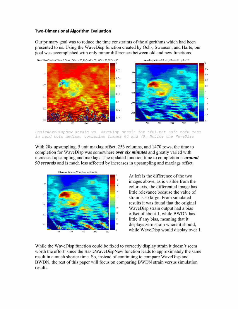
Two‐Dimensional Algorithm Evaluation Our primary goal was to reduce the time constraints of the algorithms which had been presented to us. Using the WaveDisp function created by Ochs, Swanson, and Harte, our goal was accomplished with only minor differences between old and new functions.
BasicWaveDispNew strain vs. WaveDisp strain for tfu1.mat soft tofu core in hard tofu medium, comparing frames 60 and 70. Notice the WaveDisp With 20x upsampling, 5 unit maxlag offset, 256 columns, and 1470 rows, the time to completion for WaveDisp was somewhere over six minutes and greatly varied with increased upsampling and maxlags. The updated function time to completion is around 90 seconds and is much less affected by increases in upsampling and maxlags offset.
At left is the difference of the two images above, as is visible from the color axis, the differential image has little relevance because the value of strain is so large. From simulated results it was found that the original WaveDisp strain output had a bias offset of about 1, while BWDN has little if any bias, meaning that it displays zero strain where it should, while WaveDisp would display over 1.
While the WaveDisp function could be fixed to correctly display strain it doesn’t seem worth the effort, since the BasicWaveDispNew function leads to approximately the same result in a much shorter time. So, instead of continuing to compare WaveDisp and BWDN, the rest of this paper will focus on comparing BWDN strain versus simulation results.
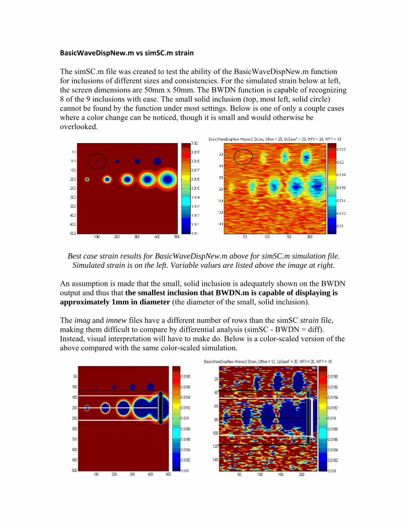
BasicWaveDispNew.m vs simSC.m strain The simSC.m file was created to test the ability of the BasicWaveDispNew.m function for inclusions of different sizes and consistencies. For the simulated strain below at left, the screen dimensions are 50mm x 50mm. The BWDN function is capable of recognizing 8 of the 9 inclusions with ease. The small solid inclusion (top, most left, solid circle) cannot be found by the function under most settings. Below is one of only a couple cases where a color change can be noticed, though it is small and would otherwise be overlooked.
Best case strain results for BasicWaveDispNew.m above for simSC.m simulation file. Simulated strain is on the left. Variable values are listed above the image at right.
An assumption is made that the small, solid inclusion is adequately shown on the BWDN output and thus that the smallest inclusion that BWDN.m is capable of displaying is approximately 1mm in diameter (the diameter of the small, solid inclusion). The imag and imnew files have a different number of rows than the simSC strain file, making them difficult to compare by differential analysis (simSC - BWDN = diff). Instead, visual interpretation will have to make do. Below is a color-scaled version of the above compared with the same color-scaled simulation.
The vertical mm/pixel of the image on the left and right at the bottom of the previous page are 0.1mm/pixel and 0.1953mm/pixel per unit respectively. A few quick measurements show the largest Gaussian inclusion has a diameter of 16mm, marked in black on both images. The diameter of the BWDN strain large Gaussian inclusion is around 10.55mm and is marked in white on both images. Comparing the expected to actual shows that there are about 2.73mm of inclusion on the top and bottom of the large Gaussian inclusion that are not recognized by BWDN. More results on this topic are presented under ‘elasticitySimImage.mat testing’ on the following page.
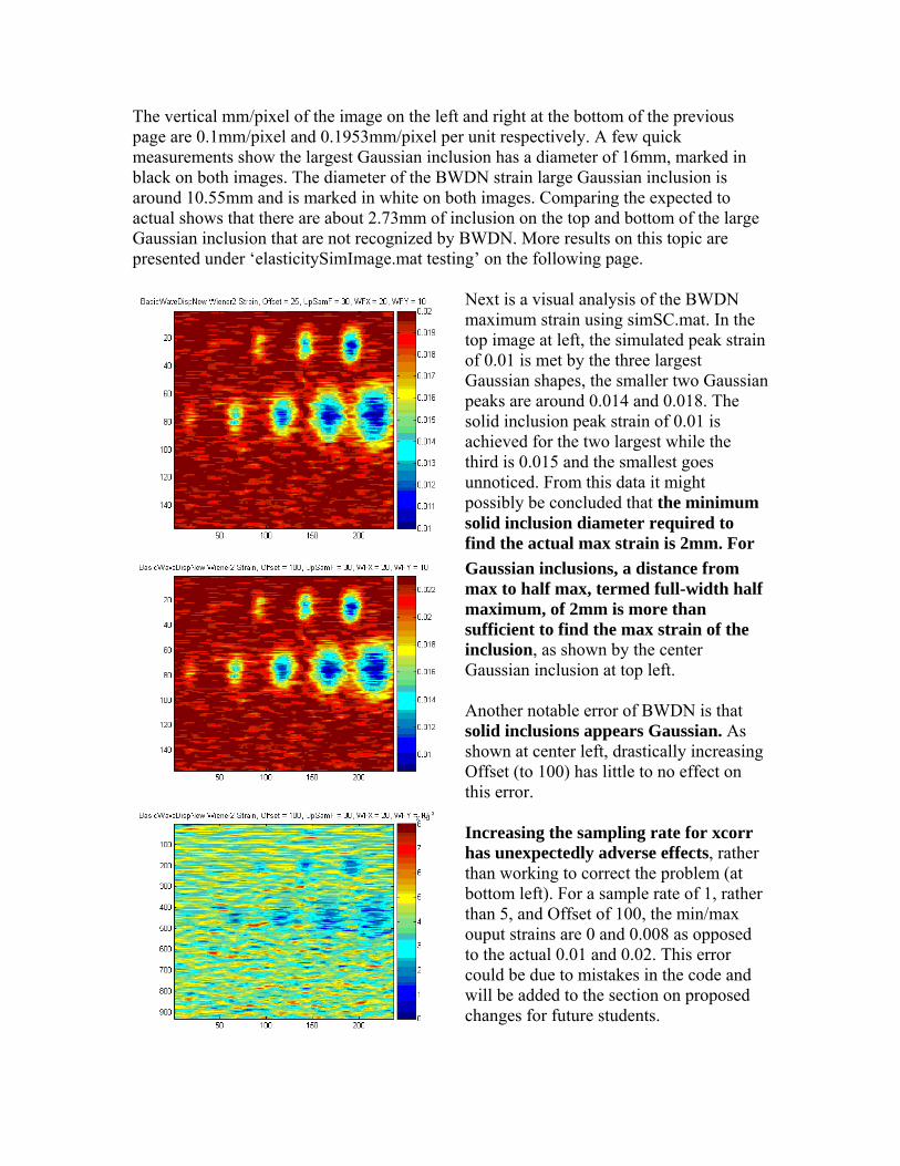
Next is a visual analysis of the BWDN maximum strain using simSC.mat. In the top image at left, the simulated peak strain of 0.01 is met by the three largest Gaussian shapes, the smaller two Gaussian peaks are around 0.014 and 0.018. The solid inclusion peak strain of 0.01 is achieved for the two largest while the third is 0.015 and the smallest goes unnoticed. From this data it might possibly be concluded that the minimum solid inclusion diameter required to find the actual max strain is 2mm. For
Gaussian inclusions, a distance from max to half max, termed full-width half maximum, of 2mm is more than sufficient to find the max strain of the inclusion, as shown by the center Gaussian inclusion at top left. Another notable error of BWDN is that solid inclusions appears Gaussian. As shown at center left, drastically increasing Offset (to 100) has little to no effect on this error. Increasing the sampling rate for xcorr has unexpectedly adverse effects, rather than working to correct the problem (at bottom left). For a sample rate of 1, rather than 5, and Offset of 100, the min/max ouput strains are 0 and 0.008 as opposed to the actual 0.01 and 0.02. This error could be due to mistakes in the code and will be added to the section on proposed changes for future students.
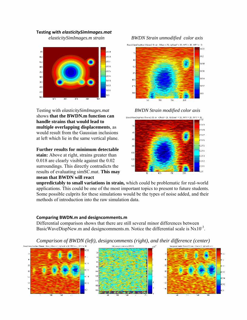
Testing with elasticitySimImages.mat elasticitySimImages.m strain BWDN Strain unmodified color axis
Testing with elasticitySimImages.mat BWDN Strain modified color axis shows that the BWDN.m function can handle strains that would lead to multiple overlapping displacements, as would result from the Gaussian inclusions at left which lie in the same vertical plane. Further results for minimum detectable stain: Above at right, strains greater than 0.018 are clearly visible against the 0.02 surroundings. This directly contradicts the results of evaluating simSC.mat. This may mean that BWDN will react unpredictably to small variations in strain, which could be problematic for real-world applications. This could be one of the most important topics to present to future students. Some possible culprits for these simulations would be the types of noise added, and their methods of introduction into the raw simulation data. Comparing BWDN.m and designcomments.m Differential comparison shows that there are still several minor differences between BasicWaveDispNew.m and designcomments.m. Notice the differential scale is Nx10-3. Comparison of BWDN (left), designcomments (right), and their difference (center)
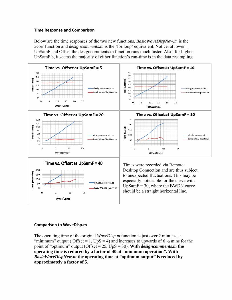
Time Response and Comparison Below are the time responses of the two new functions. BasicWaveDispNew.m is the xcorr function and designcomments.m is the ‘for loop’ equivalent. Notice, at lower UpSamF and Offset the designcomments.m function runs much faster. Also, for higher UpSamF’s, it seems the majority of either function’s run-time is in the data resampling.
Times were recorded via Remote Desktop Connection and are thus subject to unexpected fluctuations. This may be especially noticeable for the curve with UpSamF = 30, where the BWDN curve should be a straight horizontal line.
Comparison to WaveDisp.m
The operating time of the original WaveDisp.m function is just over 2 minutes at “minimum” output ( Offset = 1, UpS = 4) and increases to upwards of 6 ½ mins for the point of “optimum” output (Offset = 25, UpS = 30). With designcomments.m the operating time is reduced by a factor of 40 at “minimum operation”. With BasicWaveDispNew.m the operating time at “optimum output” is reduced by approximately a factor of 5.

Conclusion for 2‐D functions Changes to WaveDisp were to:
1) Greatly reduce operation time, by as much as 5x when set for optimum strain results.
2) Make strain results more accurate by comparing results to simulated data.
3) Add comments through designcomments.mat to help ease the understanding of next semester’s students.
Changes to blip protection were not made due to lack of time and a lack of need with simulation data. These results were not shown in this report.
Several tests were done to:
1) Determine and plot operating time with varying system parameters.
2) Test ability of BasicWaveDispNew with respect to;
a. inclusion size,
b. difference in strain,
c. solid vs. Gaussian inclusions. Many suggestions as to possible corrections to the function(s) are presented on the following page.

BasicWaveDispNew.m Goals for Future Students
1) Corrections for:
a. Minimum detectable difference in strain or reason for conflicting results between elasticitySimImages.mat and simSC.mat.
b. Minimum detectable inclusion size (about 1mm diameter solid circle).
c. Minimum inclusion size to detect true max strain (about 2mm diameter solid circle or less than 2mm full-width half maximum Gaussian). d. The gaussian appearance of solid inclusions (reasons unknown).
e. Minor differences between BasicWaveDispNew and designcomments
2) Improve Overall Accuracy, possibly through:
a. Better displacement estimation (see Basarab08 data for advanced ideas).
b. More advanced filtering
3) Blip Protection
a. Allow for offset greater than the typical wavelength with current hardware (around 4.5 pixels/period pre-upsampling) without excessive blips.
b. Improve the condition in place for when displacement exceeds user- set bounds. (Currently 2*WSpan2)
4) Determine cause for negative strains for Tofu data 1,2,3
5) Corrections if needed for multiple back-to-back frame comparisons.
6) Corrections and improvements to dim2basic.m.

Group Member’s Roles: Steven Sivewright: Improvements to the algorithms of the Spring 2008 semester’s students. Phillip Chesnut: Work and testing on one-dimensional displacement and strain algorithm. References and acknowledgements for use of other’s contributions: Algorithms from the Spring semester 2008 groups of Ochs, Swanson, and Harte (OHS) Baer, Robinson, and Wibbenmeyer (BRW), and Michaels and Watts (MW) were researched extensively prior to creation of our current algorithms. Some segments of these algorithms were used to produce our current algorithms including the process of OHS’s WaveDisp function in our own two-dimensional BasicWaveDispNew function. From MW we took note of the ‘Filter’ function to determine strain, which was used in tandem with the ‘Wiener2’ function of OHS to test the validity of each and the BWDN strain itself. Current student Patrick Vogelaar was also helpful in sharing the ability of ‘tic and toc’ and, through his parameter testing, greatly contributing to reduced operating time. Information on strain imaging applications for the Background portion of the report was found at: http://www.lp-it.de/download/overview-strain-imaging.pdf. Title: Real Time Strain Imaging Authors: Andreas Lorenz, Andreas Pesavento LP-IT Innovative Technologies GmbH, Huestrabe 5, 44787 Bochum, Germany

Appendix A xcorr explanation When using the xcorr function, each column in the cross correlation output has its own value and location. When xcorr is called by: [Corr Lag] = xcorr(x,y); where: xcorr(n) = ∑ x[m] y[m-n] m
The output Corr is a row vector of cross correlation values when the displacement matrix is displaced a certain distance m and Lag denotes the displacement in integer units of the center of the Y vector from the center of the X vector. Corr = xcorr(Lag) = ∑ x[m] y[m-Lag] m
As an example, here is how one set of Corr and Lag are determined:
X1 X2 X3 X4 X5 * * * * * * * Y1 Y2 Y3 Y4 Y5 |<----------|<---------| -2 -1 0 Figure 11 For this part of the xcorr output vector: Corr = (0*Y1 + 0*Y2) + X1*Y3 + X2*Y4 + X3*Y5 + (X4*0 + X5*0) Lag = -2 The next column of the output will be: Corr = X4*Y5 + X3*Y4 + X2*Y3 + X1*Y2 Lag = -1 The total number of columns will be 2N-1 where N is the length of the larger of functions X or Y. (The xcorr function will concatenate 0’s to the right end of the smaller function so that both functions are the same size while the Corr values remain unchanged). The max Lag value is determined from [MCorr MLag] = max(xcorr(X,Y)) Continued on next page
xcorr continued Unlike the standard xcorr outputs, MCorr is a 1x1 vector containing the maximum value of xcorr obtained. MLag is no longer the distance from the center of the first vector to the center of the second. It is now the column number of the output from which MCorr was obtained. If MLag was obtained from Figure 11 on the previous page: MCorr = Corr = X1*Y3 + X2*Y4 + X3*Y5 MLag = 3 maxlags Using the maxlags ability of the xcorr function allows one to return only a certain data range of the xcorr output rather than the entire 2N-1 range of possible values, (where N is the length of the row vector inputs). Maxlags allows the xcorr function to operate over a range of (2*maxlags + 1) centered around Lag 0 of the x input vector. This is implemented by: [Corr Lag] = xcorr(x, y, maxlags) This function will return a total of 2*maxlags + 1 output columns in the form: Corr(Lag) = xcorr(Lag) = ∑ x[m] y[m-Lag] m
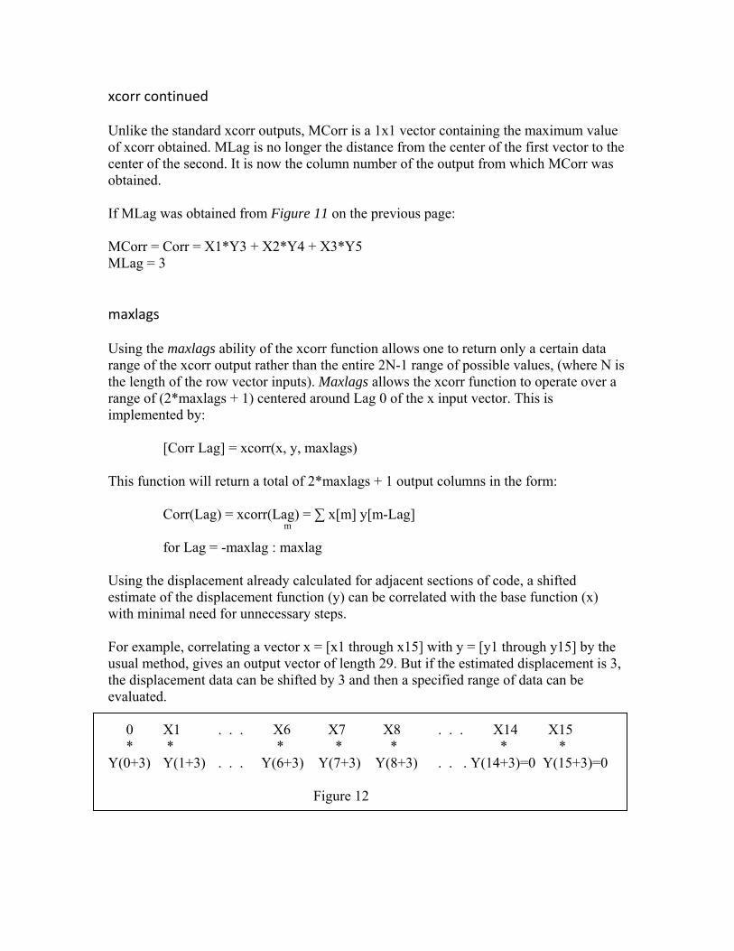
for Lag = -maxlag : maxlag Using the displacement already calculated for adjacent sections of code, a shifted estimate of the displacement function (y) can be correlated with the base function (x) with minimal need for unnecessary steps. For example, correlating a vector x = [x1 through x15] with y = [y1 through y15] by the usual method, gives an output vector of length 29. But if the estimated displacement is 3, the displacement data can be shifted by 3 and then a specified range of data can be evaluated. 0 X1 . . . X6 X7 X8 . . . X14 X15 * * * * * * * Y(0+3) Y(1+3) . . . Y(6+3) Y(7+3) Y(8+3) . . . Y(14+3)=0 Y(15+3)=0
Figure 12
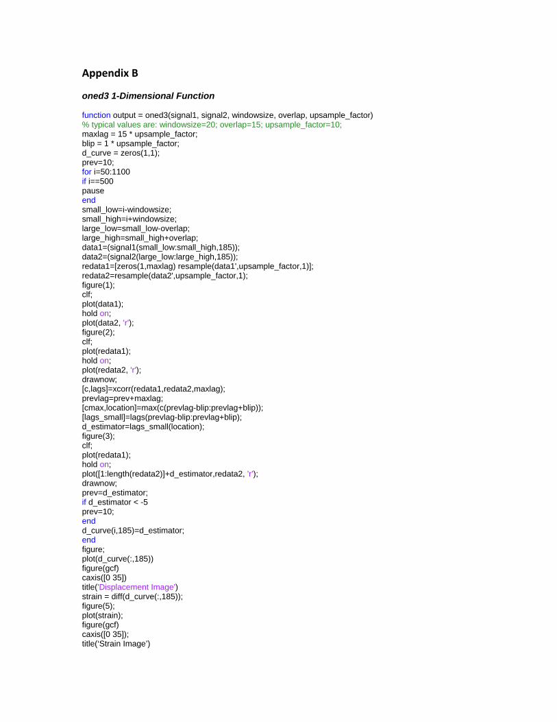
Appendix B oned3 1-Dimensional Function
function output = oned3(signal1, signal2, windowsize, overlap, upsample_factor) % typical values are: windowsize=20; overlap=15; upsample_factor=10; maxlag = 15 * upsample_factor; blip = 1 * upsample_factor; d_curve = zeros(1,1); prev=10; for i=50:1100 if i==500 pause end small_low=i-windowsize; small_high=i+windowsize; large_low=small_low-overlap; large_high=small_high+overlap; data1=(signal1(small_low:small_high,185)); data2=(signal2(large_low:large_high,185)); redata1=[zeros(1,maxlag) resample(data1',upsample_factor,1)]; redata2=resample(data2',upsample_factor,1); figure(1); clf; plot(data1); hold on; plot(data2, 'r'); figure(2); clf; plot(redata1); hold on; plot(redata2, 'r'); drawnow; [c,lags]=xcorr(redata1,redata2,maxlag); prevlag=prev+maxlag; [cmax,location]=max(c(prevlag-blip:prevlag+blip)); [lags_small]=lags(prevlag-blip:prevlag+blip); d_estimator=lags_small(location); figure(3); clf; plot(redata1); hold on; plot([1:length(redata2)]+d_estimator,redata2, 'r'); drawnow; prev=d_estimator; if d_estimator < -5 prev=10; end d_curve(i,185)=d_estimator; end figure; plot(d_curve(:,185)) figure(gcf) caxis([0 35]) title('Displacement Image') strain = diff(d_curve(:,185)); figure(5); plot(strain); figure(gcf) caxis([0 35]); title(‘Strain Image’)
designcomments.mat 2-Dimensional Function function strain = designcomments(func1, func2) % The following function creates a matrix of the displacement between two % 2-dimensional ultrasound signals, one a reference signal and the other a % signal with compression. % Feel free to change the title to something shorter. %function output = designcomments(func1,func2,xmin,xmax,ymin,ymax,wsize,WienerFilterX,WienerFilterY) %% Comment above is an alternate heading allowing several variables to be %% input from the Command Window. Any additional variables can be added to %% the list as desired. tic % Use tic and toc to return the time that a desired section of code takes to run, % the toc for this tic is at the very end of the function. xmin = 30; xmax = 1000; ymin = 1; ymax = 256; wsize = 20; UpSamF = 30; %Upsampling factor. Used for func1 and func2 resampling below. Offset = 1; % This is the number of data points (before resampling) that % is assumed as the maximum possible change in displacement. % Offset = 1 doesn't seem to be adequate, while offset = 10 % may lead to errors (if OffsetAttenuation is not used). SweepFactor = 5;% one out of every SweepFactor points of the original input % matrices will be used to measure displacement. This is % primarily to save time by reducing the amount of % calculations. A SweepFactor of 1 will give displacement % calculations at each point in the input matrix. A factor % of 10 leads to a displacement calculation for one point, % then skipping the next 9 points and finding the displacement of the 10th point, etc. % The function is very sensitive to changes in this parameter. OffsetAttenuation = 30; % This factor is used to tweak maxlags (immediately % below) to a desired range. It could be set to 1 and % ignored if desired. Typically OffsetAttenuation = UpSamF. WienerFilterX = 20; % These two variables are for the Wiener2 filter used WienerFilterY = 10; % just before differentiating to recieve a strain image. FirstFrame = 79; % first frame for multi-frame comparison, must be enabled below as well FinalFrame = 80; % final frame for multi-frame comparison, must be enabled below as well FrameSteps = 1; % number of frames between comparison sets, 5 gives 85 vs. 90, 90 vs. 95, etc. FramebyFrameEnable=0; %set to 1 to enable, must still be altered below for certain datasets. FramebyFramePics=0; %set to 1 to enable outputs after each frame to frame comparison. % Recommended values for 1559x256 input matrices is: % xmin = 30; % xmin of 30 should be the minimum allowable xmin % xmax = 1500; % avoid xmax near the input row size, will cause errors. % ymin = 1; % no requirements for ymin besides absolute size of dataset % ymax = 256; % no requirements for ymax besides absolute size of dataset % wsize = 20; % determines the size of the correlation window in xcorr. % UpSamF = 20; % reasonable value of UpSamF for optimum strain results. % Offset = 5; % small value of Offset, if Offset Attenuation = UpSamF % SweepFactor = 5; % Little testing was done for other SweepFactor values. % WienerFilterX = 20 % uncertain actually, though a value around 20 gives decent results % WienerFilterY = 15 % same as above, WSpan1 = ceil((wsize / 2)*UpSamF); %Sizing for window around center point. WSpan2 = ceil(1.5 * WSpan1); %Sizing of comparison window size. % WSpan's are needed for the initial xcorr displacement calculation, i.e. % line 1, sample 1. maxlags = ceil(Offset*UpSamF/OffsetAttenuation); % maxlags is the upsampled offset. It is named after an % ability of the xcorr function because it serves the % sampe purpose.
maxc = 2*maxlags+1; % for xcorr with maxlags of N, there will be 2*N+1 entries % in the xcorr output vector. See help section for more on % xcorr and maxlags. MDisp(1:(ymax-ymin),1:ceil((xmax-xmin)/SweepFactor)+1) = 0; % This is the output matrix, which is being initialized to % all zeros; %% Beginning of function core if FramebyFramePics==1 figure; % set up figure for frame to frame analysis. end for n = 1:FrameSteps:FinalFrame-FirstFrame %% This loop allows multiple frames (i.e. b_data001, b_data002, etc.) %% to be compared back to back and the results added together. It %% should be helpful when comparing distant frames (i.e. 40 vs. 100) %% which would otherwise not turn out well. The outcome of implementing %% this loop is somewhat untested and may contain errors. %%vvvvvvvvvvvvvvvvvvvvvvvvvvvvvvvvvvvvvvvvvvvvvvvv% if FramebyFrameEnable == 1 k = sprintf('func1 = b_data%03d;', FirstFrame+n-1); l = sprintf('func2 = b_data%03d;', FirstFrame+FrameSteps+n-1); eval(k); eval(l); end %%^^^^^^^^^^^^^^^^^^^^^^^^^^^^^^^^^^^^^^^^^^^^^^^^% %% Unfortunately, as it stands the section above %% must be altered inside the editor when using different data (i.e. %% tfu1,tfu2,etc.). To do this, change the word b_data to whatever %% heading is required for the particular dataset. Make sure to leave %% the %03d alone as is it is what increments to allow the use of %% different numbered frames. P.S. make sure not to input %% b_data001%03d, but instead b_data%03d and set first frame to 1. %% Special Note: the multi-frame comparison has no benefit for %% simulation datasets which consist of only 2 frames. line = 0; % Initial incrementation for the line number, increments one unit at a % time. Used as a reference for the location of storage in the output % displacement matrix. [rows cols] = size(func1); if rows > cols %Inverting function allows for multiple BaseR2 = (resample(func1,UpSamF,1))'; %function types as inputs. Sine waves and DispR2 = (resample(func2,UpSamF,1))'; %2 dimensional images can both be processed. else BaseR2 = resample(func1,UpSamF,1); DispR2 = resample(func2,UpSamF,1); end %This loop performs cross correlation of func1 and func2 for wsize samples. %This loop also has previous data comparison to prevent spikes in %displacement imaging. for ysweep = ymin:ymax line = line+1; sample = 0; for xsweep = xmin*UpSamF-(UpSamF-1):SweepFactor*UpSamF:xmax*UpSamF-(UpSamF-1) % xsweep range of xmin:SweepFactor:xmax is converted to % upsampled form. sample = sample +1; %The following is the algorithm for spike prevention in the %displacement calculations. %Order is, n~=1 --> line~=1 --> sample==1 --> sample~=1 % --> line==1 --> sample==1 --> sample~=1 % n==1 --> line~=1 --> sample==1 --> sample~=1 % --> line==1 --> sample==1 --> sample~=1 % Most comments are in n==1 secion at bottom if n~=1 % if not the comparison of the first two inputs. (e.g. If % currently comparing datasets 2 and 3 of a group of % three, where 3 is a compressed version of signal 2 % and signal 2 is a compressed version of signal 1),
% this section of the loops will incorporate into the % displacement estimation the output obtained from % previously comparing datasets 1 and 2. if line ~=1 % if not the first line of data ( lines are 1:(ymax-ymin) ) MLag = ceil((MDisp(line,sample,n-1)+MDisp(line-1,sample,n))/2); % Set MLag to an average of adjacent points already collected. %Prev displacement set to average of previous %line and previous frame (which will be zero if multiple frames not being used). if sample ==1 % if the first data point in new line MLag = ceil((MDisp(line-1,1,n) + MDisp(line,1,n-1))/2); for c = 1:maxc Lag(1,c) = sum([zeros(1,maxlags) BaseR2(ysweep, xsweep-WSpan1:xsweep+WSpan1) zeros(1,maxlags)].*[zeros(1,c-1) DispR2(ysweep,(xsweep-WSpan1-MLag):(xsweep+WSpan1-MLag)) zeros(1,maxc-c)]); end [TCorr, TLag] = max(Lag); elseif MLag <= -2*WSpan2 % Prevents out of range low comparisons. %%Lag(1,1) = sum(BaseR2(ysweep, xsweep-WSpan1:xsweep+WSpan1).*DispR2(ysweep, xsweep-WSpan1+2*WSpan2 : xsweep+WSpan1+2*WSpan2)); TLag = maxlags+2; elseif MLag >= 2*WSpan2 % Prevents out of range high. %Lag(1,1) = sum(BaseR2(ysweep, xsweep-WSpan1:xsweep+WSpan1).*DispR2(ysweep, (xsweep-WSpan1-2*WSpan2): xsweep+WSpan1-2*WSpan2)); TLag = maxlags; else % Ideal situation for c = 1:maxc Lag(1,c) = sum([zeros(1,maxlags) BaseR2(ysweep, xsweep-WSpan1:xsweep+WSpan1) zeros(1,maxlags)].*[zeros(1,c-1) DispR2(ysweep,(xsweep-(WSpan1)-MLag):(xsweep+(WSpan1)-MLag)) zeros(1,maxc-c)]); end [TCorr, TLag] = max(Lag); end % end else % if line ==1 if sample==1 MLag = MDisp(1,1,n-1); %Reference for first row displacement values. for c = 1:maxc Lag(1,c) = sum([zeros(1,maxlags) BaseR2(ysweep, xsweep-WSpan1:xsweep+WSpan1) zeros(1,maxlags)].*[zeros(1,c-1) DispR2(ysweep,(xsweep-(WSpan1)-MLag):(xsweep+(WSpan1)-MLag)) zeros(1,maxc-c)]); end [TCorr, TLag] = max(Lag); elseif MLag <= -2*WSpan2 %Prevents out of range low comparisons. %Lag(1,1) = sum(BaseR2(ysweep, xsweep-WSpan1:xsweep+WSpan1).*DispR2(ysweep, xsweep-WSpan1+2*WSpan2 : xsweep+WSpan1+2*WSpan2)); TLag = maxlags; elseif MLag >= 2*WSpan2 %Prevents out of range high. %Lag(1,1) = sum(BaseR2(ysweep, xsweep-WSpan1:xsweep+WSpan1).*DispR2(ysweep, (xsweep-WSpan1-2*WSpan2): xsweep+WSpan1-2*WSpan2)); TLag = maxlags+2; else %Normal previous point comparison. for c = 1:maxc Lag(1,c) = sum([zeros(1,maxlags) BaseR2(ysweep, xsweep-WSpan1:xsweep+WSpan1) zeros(1,maxlags)].*[zeros(1,c-1) DispR2(ysweep,(xsweep-(WSpan1)-MLag):(xsweep+(WSpan1)-MLag)) zeros(1,maxc-c)]); end [TCorr, TLag] = max(Lag); end end MLag = TLag - 1 - maxlags + MLag; MDisp(line,sample,n) = MLag; %Generates displacement matrix. else % if n==1, meaning it is the comparison of the first two frames. % n==1 follows the same processes as n~=1 but % does not incorporate the displacement of the point in % question for the last set of frames compared. if line ~=1 %For both previous point vertical and horizontal comparison. MLag = ceil((MDisp(line-1,sample,n) + MLag)/2); % Prev displacement is set as average of % previous line (immediately above) and % previous sample (immediately to the left) if sample ==1 %For only previous point vertical comparison.
MLag = MDisp(line-1,1,n); %Reference for first row displacement values. for c = 1:maxc Lag(1,c) = sum([zeros(1,maxlags) BaseR2(ysweep, xsweep-WSpan1:xsweep+WSpan1) zeros(1,maxlags)].*[zeros(1,c-1) DispR2(ysweep,(xsweep-(WSpan1)-MLag):(xsweep+(WSpan1)-MLag)) zeros(1,maxc-c)]); end [TCorr, TLag] = max(Lag); elseif MLag <= -2*WSpan2 %Prevents out of range low comparisons. %Lag(1,1) = sum(BaseR2(ysweep, xsweep-WSpan1:xsweep+WSpan1).*DispR2(ysweep, xsweep-WSpan1+2*WSpan2 : xsweep+WSpan1+2*WSpan2)); TLag = maxlags+2; elseif MLag >= 2*WSpan2 %Prevents out of range high. %Lag(1,1) = sum(BaseR2(ysweep, xsweep-WSpan1:xsweep+WSpan1).*DispR2(ysweep, (xsweep-WSpan1-2*WSpan2): xsweep+WSpan1-2*WSpan2)); TLag = maxlags; else %% Ideal situation for c = 1:maxc Lag(1,c) = sum([zeros(1,maxlags) BaseR2(ysweep, xsweep-WSpan1:xsweep+WSpan1) zeros(1,maxlags)].*[zeros(1,c-1) DispR2(ysweep,(xsweep-(WSpan1)-MLag):(xsweep+(WSpan1)-MLag)) zeros(1,maxc-c)]); end % Above is the same process as for n==1, line==1, % sample==1 except that the previous displacement % used for shifting incorporates prev row and % column displacments. [TCorr, TLag] = max(Lag); end else %% if line ==1, uses the same processes described above, but % without incorporating the previous line displacement % into the current MLag (i.e. leaves out % MDisp(line-1,sample,n). if sample==1 %Reference for first row displacement values. [TCorr, TLag] = max(xcorr([zeros(1,ceil(WSpan1/2)) BaseR2(ysweep, xsweep-WSpan1:xsweep+WSpan1) zeros(1,ceil(WSpan1/2))], [zeros(1,(ceil(WSpan1/2) - floor(WSpan1/2))) DispR2(ysweep, xsweep-WSpan2:xsweep+WSpan2)])); MLag = -1*(2*WSpan2-maxlags); elseif MLag <= -2*WSpan2 %Prevents out of range low comparisons. % Bounds are -2*WSpan2 to 2*WSpan2, this bound selection was arbitrary. %Lag(1,1) = sum(BaseR2(ysweep, xsweep-WSpan1:xsweep+WSpan1).*DispR2(ysweep, xsweep-WSpan1+2*WSpan2 : xsweep+WSpan1+2*WSpan2)); TLag = maxlags+2; % If displacement is below desirable range (and % therefore assumed a blip) the previous % section computes the displacement at the % negative rail and sets up TLag to cause % MLag to be one unit less than the previous, so it can % run through the ideal case loop on the next % pass. This process may be questionable. % Note: the Lag(1,1)=... eqn is unnecessary % here since TLag is set to maxlags+2 regardless of the % Lag output. The eqn is left here as a % starting point in case changes need to be % made to improve this situation. elseif MLag >= 2*WSpan2 %Prevents out of range high. % Similar process as the step above but for % displacement in the opposite direction. %Lag(1,1) = sum(BaseR2(ysweep, xsweep-WSpan1:xsweep+WSpan1).*DispR2(ysweep, (xsweep-WSpan1-2*WSpan2): xsweep+WSpan1-2*WSpan2)); TLag = maxlags; else %Normal previous point comparison. for c = 1:maxc Lag(1,c) = sum([zeros(1,maxlags) BaseR2(ysweep, xsweep-WSpan1:xsweep+WSpan1) zeros(1,maxlags)].*[zeros(1,c-1) DispR2(ysweep,(xsweep-(WSpan1)-MLag):(xsweep+(WSpan1)-MLag)) zeros(1,maxc-c)]); end %\--------------Base (stationary) xcorr input with prev displacement----------------------/ \----------------------Displacement (sliding) xcorr input------------------------/ % The above For loop approximates xcorr with % maxlags by multiplying two signals and % summing the results. This for loop cuts out a % lot of unnecessary calculations of xcorr with
% maxlags though the process can still be % improved. The above can be approximated as: % xcorr(base(y,x-window+DisplacementEstimate:x+window+DisplacementEstimate), displacement(y,x-window:x+window),maxlags); [TCorr, TLag] = max(Lag); % TLag is the estimation of true displacement % between the two signals (The point where the % maximum sum of multiplications occurs). % TCorr is irrelevant. It must be included to % find the location TLag. end end MLag = TLag - 1 - maxlags + MLag; % To calculate actual displacement from previous MDisp(line,sample,n) = MLag; %Generates displacement matrix. end end end %% Below plots a displacement image for each frame-to-frame comparison when %% comparing multiple frames. if FramebyFramePics==1 clf; if rows > cols %Reverts axis back to original orientation. output = -(MDisp(:,:,n)'/UpSamF); else output = -(MDisp(:,:,n)/UpSamF); end imagesc(output); heading = sprintf('designcomments Displacement Plot %d', n); title(heading) drawnow; end end %% End of core for loops if rows > cols %Reverts axis back to original orientation. output = (-1*(MDisp'/UpSamF)); %% Negative signs were a quick fix when it else %% was discovered simulation outputs were output = -1*(MDisp/UpSamF); %% coming out negative. end figure imagesc(output); text = sprintf('designcomments Displacement, Offset = %d, UpSamF = %d', Offset, UpSamF); title(text) colorbar; [rows, cols] = size(output); output2 = wiener2(output,[WienerFilterX WienerFilterY]); %Performs wiener2 averaging for filtering noise and removes figure %distorted area from wiener2 function. imagesc(output2(WienerFilterX:rows-WienerFilterX,WienerFilterY:cols-WienerFilterY)); text = sprintf('designcomments Wiener2 Displacement, Offset = %d, UpSamF = %d', Offset, UpSamF); title(text) colorbar; strain=diff(output2); figure imagesc(strain(WienerFilterX:rows-WienerFilterX,WienerFilterY:cols-WienerFilterY)); text = sprintf('designcomments Wiener2 Strain, Offset = %d, UpSamF = %d', Offset, UpSamF); title(text) colorbar; WindowSize=20; average=filter(ones(1,WindowSize)/WindowSize,1,output); m=diff(average); [rows,cols]=size(m); figure imagesc(m(WindowSize:rows,:)); text = sprintf('designcomments "Filter" Strain, Offset = %d, UpSamF = %d', Offset, UpSamF); title(text) colorbar; toc %% end of designcomments.m function, tic to toc measures time from start to finish.
BasicWaveDispNew.mat 2-Dimensional Function function strain = BasicWaveDispNew(func2, func1) tic xmin = 30; xmax = 1000; ymin = 1; ymax = 256; wsize = 20; WienerFilterX = 20; WienerFilterY = 10; % recommended xmax at least 15 less than column size [rows cols] = size(func1); %Determines size of input base function. UpSamF = 30; %Upsampling ratio factor. WSpan1 = ceil((wsize / 2)*UpSamF); %Sizing for window around center point. WSpan2 = ceil(1.5 * WSpan1); %Sizing of comparison window size. SweepFactor = 5; Offset = 25; OffsetAttenuation = 30; maxlags = ceil(Offset*UpSamF/OffsetAttenuation); MDisp(1:(ymax-ymin),1:ceil((xmax-xmin)/SweepFactor)+1) = 0; line = 0; if rows > cols %Inverting function allows for multiple BaseR2 = (resample(func1,UpSamF,1))'; %function types as inputs. Sine waves and DispR2 = (resample(func2,UpSamF,1))'; %2 dimensional images can both be processed. else BaseR2 = resample(func1,UpSamF,1); DispR2 = resample(func2,UpSamF,1); end %This loop performs cross correlation of func1 and func2 for wsize samples. %This loop also has previous data comparison to prevent spikes in %displacement imaging. for ysweep = ymin:ymax line = line+1; sample = 0; for xsweep = xmin*UpSamF-(UpSamF-1):SweepFactor*UpSamF:xmax*UpSamF-(UpSamF-1) %Resamples and performs cross correlation of input signals. sample = sample +1; %The following is the algorithm for spike prevention in the %displacement calculations. if line ~=1 %For both previous point vertical and horizontal comparison. MLag = ceil((MLag + MDisp(line-1,sample)) / 2); if sample ==1 %For only previous point vertical comparison. MLag = MDisp(line-1,1); %Reference for first row displacement values. [TCorr, TLag] = max(xcorr(BaseR2(ysweep, xsweep-WSpan1+MLag:xsweep+WSpan1+MLag), DispR2(ysweep,(xsweep-(WSpan1)):(xsweep+(WSpan1))),maxlags)); elseif MLag <= -2*WSpan2 %Prevents out of range low comparisons. [TCorr, TLag] = max(xcorr(BaseR2(ysweep, xsweep-WSpan1:xsweep+WSpan1), DispR2(ysweep, xsweep-WSpan1+2*WSpan2 : xsweep+WSpan1+2*WSpan2),0)); elseif MLag >= 2*WSpan2 %Prevents out of range high. [TCorr, TLag] = max(xcorr(BaseR2(ysweep, xsweep-WSpan1:xsweep+WSpan1), DispR2(ysweep, (xsweep-WSpan1-2*WSpan2): xsweep+WSpan1-2*WSpan2),0)); else %% Ideal situation [TCorr, TLag] = max(xcorr(BaseR2(ysweep, xsweep-WSpan1+MLag:xsweep+WSpan1+MLag), DispR2(ysweep,(xsweep-(WSpan1)):(xsweep+(WSpan1))),maxlags)); end else %% if line ==1 if sample==1
[TCorr, TLag] = max(xcorr([zeros(1,ceil(WSpan1/2)) BaseR2(ysweep, xsweep-WSpan1:xsweep+WSpan1) zeros(1,ceil(WSpan1/2))], [zeros(1,(ceil(WSpan1/2) - floor(WSpan1/2))) DispR2(ysweep, xsweep-WSpan2:xsweep+WSpan2)])); MLag = -1*(2*WSpan2-maxlags); elseif MLag <= -2*WSpan2 %Prevents out of range low comparisons. [TCorr, TLag] = max(xcorr(BaseR2(ysweep, xsweep-WSpan1:xsweep+WSpan1), DispR2(ysweep, xsweep-WSpan1+2*WSpan2 : xsweep+WSpan1+2*WSpan2),0)); elseif MLag >= 2*WSpan2 %Prevents out of range high. [TCorr, TLag] = max(xcorr(BaseR2(ysweep, xsweep-WSpan1:xsweep+WSpan1), DispR2(ysweep, (xsweep-WSpan1-2*WSpan2): xsweep+WSpan1-2*WSpan2),0)); else %Normal previous point comparison. [TCorr, TLag] = max(xcorr(BaseR2(ysweep, xsweep-WSpan1+MLag:xsweep+WSpan1+MLag), DispR2(ysweep,(xsweep-(WSpan1)):(xsweep+(WSpan1))),maxlags)); end end MLag = TLag - maxlags-1 + MLag; MDisp(line,sample) = MLag; %Generates displacement matrix. end end %MDisp = wiener2(MDisp); %Performs wiener2 averaging for filtering noise. %Removes distorted area from wiener2 function. Function pads original %image with zeros, so outer rows and columns have stored values. if rows > cols %Reverts axis back to original orientation. output = ((MDisp'/UpSamF)); else output = (MDisp/UpSamF); end figure imagesc(output); text = sprintf('BasicWaveDispNew Displacement, Offset = %d, UpSamF = %d', Offset, UpSamF); title(text) colorbar; [rows, cols] = size(output); output2 = wiener2(output,[WienerFilterX WienerFilterY]); figure imagesc(output2(WienerFilterX:rows-WienerFilterX,WienerFilterY:cols-WienerFilterY)); text = sprintf('BasicWaveDispNew Wiener2 Displacement, Offset = %d, UpSamF = %d, WFX= %d, WFY = %d', Offset, UpSamF, WienerFilterX, WienerFilterY); title(text) colorbar; strain=diff(output2); figure imagesc(strain(WienerFilterX:rows-WienerFilterX,WienerFilterY:cols-WienerFilterY)); text = sprintf('BasicWaveDispNew Wiener2 Strain, Offset = %d, UpSamF = %d, WFX = %d, WFY = %d', Offset, UpSamF, WienerFilterX, WienerFilterY); title(text) colorbar; WindowSize=20; average=filter(ones(1,WindowSize)/WindowSize,1,output); m=diff(average); [rows,cols]=size(m); figure imagesc(m(WindowSize:rows,:)); text = sprintf('BasicWaveDispNew "Filter" Strain, Offset = %d, UpSamF = %d', Offset, UpSamF); title(text) colorbar; toc %End of BasicWaveDispNew.mat function
dim2basic.mat 2-Dimensional Function % Does not work correctly but is presented as an example and to make corrections. function output = dim2basic(func1,func2) tic xmin = 50; xmax = 215; ymin = 50; ymax = 965; wsize = 5; UpSamFx = 5; UpSamFy = 5; WSpan1 = ceil((wsize / 2)*UpSamFx); WSpan2 = ceil(1.5 * WSpan1); WienerFilterX = 20; WienerFilterY = 15; [rows cols] = size(func1); SweepFactorX = 1; SweepFactorY = 5; Offset = 1+WSpan1; OffsetA = 3+WSpan1; StartingOffset = WSpan2; StartingOffsetA = WSpan2+20; disp(ceil((ymax-ymin)/SweepFactorY)+1,ceil((xmax-xmin)/SweepFactorX)+1,2)=zeros; BaseR2 = resample((resample(func1,UpSamFy,1))',UpSamFx,1)'; DispR2 = resample((resample(func2,UpSamFy,1))',UpSamFx,1)'; [rows2 cols2] = size(BaseR2); dispcenter= [ceil((2*wsize*UpSamFy+OffsetA+Offset-1)/2) ceil((2*wsize*UpSamFx+OffsetA+Offset-1)/2)]; %% Center of xcorr2 output window, used as a reference to find displacement %% about the center of the two aligned signal windows. Drow = 0; %% Incrementer for Rows for ysweep = UpSamFy*ymin-(UpSamFy-1):UpSamFy*SweepFactorY:ymax*UpSamFy-(UpSamFy-1) Drow = Drow+1; Dcolumn = 0; %% Incrementer for Columns for xsweep = UpSamFx*xmin-(UpSamFx-1):UpSamFx*SweepFactorX:xmax*UpSamFx-(UpSamFx-1) Dcolumn = Dcolumn+1; if Drow == 1 if Dcolumn == 1 C = xcorr2(BaseR2((ysweep-StartingOffsetA):(ysweep+StartingOffsetA),(xsweep-StartingOffsetA):(xsweep+StartingOffsetA)), DispR2(ysweep-StartingOffset:ysweep+StartingOffset,xsweep-StartingOffset:xsweep+StartingOffset));
%% C= xcorr2(Base Window, Disp Window); [val, loc] = max(C); [val2,loc2] = max(val); %% Both above used to find x and y max locations which are %% input below disp1 = [loc(loc2),loc2]; disp(Drow,Dcolumn,1:2) = disp1(1,1:2)-dispcenter; %% Because max starts from 1 and counts up, subtract dispcenter %% to get a value of zero when Base and Disp are alligned, %% positive or negative depending on disallignment. else C = xcorr2(BaseR2((ysweep-OffsetA+disp(Drow,Dcolumn-1,1)):(ysweep+OffsetA+disp(Drow,Dcolumn-1,1)),(xsweep-OffsetA+disp(Drow,Dcolumn-1,2)):(xsweep+OffsetA+disp(Drow,Dcolumn-1,2))), DispR2((ysweep-Offset):ysweep+Offset,xsweep-Offset:xsweep+Offset)); %% C = xcorr2(Base Window w/ displacement estimate, Disp Window); [val, loc] = max(C); [val2,loc2] = max(val); disp1 = [loc(loc2),loc2]; disp(Drow,Dcolumn,1:2) = disp1(1,1:2)-dispcenter; end else if Dcolumn == 1 %% Broken down for ease of understanding x=BaseR2((ysweep-OffsetA+disp(Drow-1,Dcolumn,1)):(ysweep+OffsetA+disp(Drow-1,Dcolumn,1)),(xsweep-OffsetA+disp(Drow-1,Dcolumn,2):(xsweep+OffsetA+disp(Drow-1,Dcolumn,2)))); %% x = Base Window w/ Displacement Estimation y=DispR2((ysweep-Offset):ysweep+Offset,xsweep-Offset:xsweep+Offset); %% y = Disp Window C = xcorr2(x,y); %% C = xcorr2 [val, loc] = max(C); [val2,loc2] = max(val); disp1 = [loc(loc2),loc2]; disp(Drow,Dcolumn,1:2) = disp1(1,1:2)-dispcenter; else C = xcorr2(BaseR2((ysweep-OffsetA+ceil((disp(Drow-1,Dcolumn,1)+disp(Drow,Dcolumn-1,1))/2)):(ysweep+OffsetA+ceil((disp(Drow-1,Dcolumn,1)+disp(Drow,Dcolumn-1,1))/2)),(xsweep-OffsetA+ceil((disp(Drow-1,Dcolumn,2)+disp(Drow,Dcolumn-1,2))/2)):(xsweep+OffsetA+ceil((disp(Drow-1,Dcolumn,2)+disp(Drow,Dcolumn-1,2))/2))), DispR2((ysweep-Offset):ysweep+Offset,xsweep-Offset:xsweep+Offset)); [val, loc] = max(C);
[val2,loc2] = max(val); disp1 = [loc(loc2),loc2]; disp(Drow,Dcolumn,1:2) = disp1(1,1:2)-dispcenter; end end end end outputaxial = disp(:,:,1)/UpSamFx; outputlateral = disp(:,:,2)/UpSamFy; figure; imagesc (outputaxial); text=sprintf('dim2basic Axial Displacement'); title(text) colorbar; figure; imagesc (outputlateral); text = sprintf('dim2basic Lateral Displacement') title(text) colorbar; [rows, cols] = size(outputaxial); outputaxial2 = wiener2(outputaxial,[WienerFilterX WienerFilterY]); figure imagesc(outputaxial2(WienerFilterX:rows-WienerFilterX,WienerFilterY:cols-WienerFilterY)); text = sprintf('dim2basic Wiener2 Axial Displacement'); title(text) colorbar; x=diff(outputaxial2); figure imagesc(x(WienerFilterX:rows-WienerFilterX,WienerFilterY:cols-WienerFilterY)); text = sprintf('dim2basic Wiener2 Axial Strain'); title(text) colorbar; [rows, cols] = size(outputlateral); outputlateral2 = wiener2(outputlateral,[WienerFilterX WienerFilterY]); figure imagesc(outputlateral2(WienerFilterX:rows-WienerFilterX,WienerFilterY:cols-WienerFilterY)); text = sprintf('dim2basic Wiener2 Lateral Displacement'); title(text) colorbar; y=diff(outputlateral2); figure imagesc(y(WienerFilterX:rows-WienerFilterX,WienerFilterY:cols-WienerFilterY)); text = sprintf('dim2basic Wiener2 Lateral Strain'); title(text) colorbar; toc % End of dim2basic.mat