Comput. Methods Appl. Mech. Engrg. 198 (2009) 1368–1388

Contents lists available at ScienceDirect

Comput. Methods Appl. Mech. Engrg.

journal homepage: www.elsevier .com/locate /cma

New approximations of external acoustic–structural interactions: Derivationand evaluation

Moonseok Lee a, Youn-Sik Park a, Youngjin Park a, K.C. Park b,*

a Center for Noise and Vibration Control and Department of Mechanical Engineering, Korea Advanced Institute of Science and Technology, 335 Gwahangno,Yuseong-gu,Daejeon 305-701, Republic of Koreab Center for Aerospace Structures and Department of Aerospace Engineering Sciences, University of Colorado at Boulder, CO 80309-429, USA

a r t i c l e i n f o a b s t r a c t

Article history:Received 8 June 2008Received in revised form 4 December 2008Accepted 5 December 2008Available online 24 December 2008

Keywords:External acousticsStructure–acoustic interactionsRetarded and advanced acoustic potential

0045-7825/$ - see front matter � 2009 Elsevier B.V. Adoi:10.1016/j.cma.2008.12.003

* Corresponding author.E-mail address: kcpark@colorado.edu (K.C. Park).

New approximate models for external acoustics interacting with flexible structures are developed. Thebasic form of the present models is obtained by a combination of the Laplace-transformed retardedand advanced potentials with the weighting parameter as part of the model equation. It is shown thatthe maximum attainable time-derivative of convergent approximate models is two, hence any attemptto include higher orders will lead to non-convergent models. The present external acoustic model isimplemented and interfaced with a finite element structural analyzer for the transient response analysisof submerged spherical and cylindrical shells subjected to a series of incident waves. Comparisons of thepresent results with the classical analytical solutions and the Doubly Asymptotic Approximations (DAAs)show that proposed model offers improved accuracy especially for early-time responses, exhibits compu-tational robustness, and maintains the impulse response consistency that are desirable for inverse prob-lems. The present model is applied for a shock response correlation of an experimental complex ringcylinder, which demonstrates the applicability of the proposed approximate model to practical engineer-ing problems.

� 2009 Elsevier B.V. All rights reserved.

1. Introduction

Computationally tractable models of external acoustic fieldsinteracting with flexible structures have received intense interestover the past three decades. A dominant approach adopted in thedevelopment of external acoustic–structure interaction modelshas been to improve the classical plane wave approximation mod-els [1–6]. A computational advantage of these models accrues fromtheir implementation involving boundary integrals evaluated onlyover the interaction surfaces. It should be mentioned that, in a par-allel effort, the finite element-based approach has also been pur-sued. As our focus is on the use of Kirchhoff’s pressure retardedpotential for constructing approximate interaction models, we willnot dwell on the finite element models that require discretizationof the pressure field volumes and not interaction surfaces, and in-stead we refer to a recent excellent article [7] and references there-in. Regardless of interaction models one may adopt, the fidelity ofvarious approximate interaction models are evaluated by compar-ing the results obtained by the approximate models with the cor-responding analytical solutions that are obtained either by theretarded acoustic potential equation or the continuum wave equa-tion [3,8].

ll rights reserved.

One of the computationally tractable boundary element-basedapproximate acoustic–structure interaction equations is the Dou-bly Asymptotic Approximations (DAAs) proposed by Geers andco-researchers [4]. In deriving their DAA models, the two limitingcases have been modeled: early-time approximation (ETA) andlate-time approximation (LTA) by employing the initial-value andfinal-value theorems of the Laplace transform to the series expan-sion terms of the Kirchhoff’s spherical acoustic integral wave equa-tion [5]. The first or second-order DAA models are then constructedby matching the model impedances with the ETA and LTA limits.The DAA models have proved to be adequate for characterizingthe fluid acoustic radiation damping affecting the structural re-sponses that are dominated by low-frequency components. Conse-quently, they have been used as a production external acousticanalyzer that is interfaced with several commercial structural anal-ysis codes [9].

When one focuses on the pressure field modeling, not only thepressure magnitudes but also its phase information have to be ob-tained accurately. This is especially true for identifying soundsources as well as sound intensities. For example, a careful exam-ination of most existing approximate models for ideal structuralgeometries, when compared with the exact models obtained viaKirchhoff’s formula, reveals that the dominant acoustic scatteringpressure modes are often not represented. Hence, most existingapproximate models, while adequate for structural response

M. Lee et al. / Comput. Methods Appl. Mech. Engrg. 198 (2009) 1368–1388 1369

calculations, may not be applicable to inverse acoustics problemswherein the primary objective is to identify the sound sources.

This has motivated the present authors to develop acoustic mod-els that can capture predominant acoustic modes, as distinct fromstructural modes, and yet that are computationally attractive. Fromthe theoretical point of view, the well-known Kirchhoff’s retardedpotential equation may be considered as the foundation of all theexisting approximate models. Under this premise, different approx-imate acoustic models originate from the different approximationsof the retarded (or delayed) operator. As shown in the present pa-per, a straightforward derivation of a second-order approximatepressure equations from the retarded potential leads to unstablemodels, unless one invokes an elaborate procedure akin to the der-ivation of the second-order DAA2. A careful examination of theDAA2, however, revealed that the discrete DAA2 model fails to rep-resent the impulse impedance. The spherical modal version of theDAA2 does possess the correct initial impulse impedance; however,it is not applicable to general interaction surfaces as it is a sphericalmodal model. We hold the view that the correct impulse impedanceproperty is an important desirable property if approximate pres-sure interaction models are to be adopted for acoustic pressureidentification applications. As detailed in the next section, after anexhausting series of attempts the present authors have concludedthat it would be unlikely, if not impossible, to develop stable, con-vergent and high-order accurate pressure approximations employ-ing the retarded pressure potential alone. This reinforces theinventiveness of the doubly asymptotic matching procedure thathad been so successfully exploited by Geers and his colleagues [4].

To break this impasse, viz., the inability to develop stable, moreaccurate and computationally tractable pressure approximationsfrom the retarded potential alone, we have made a key departurefrom conventional paradigm. In the present paper, we employ aweighted combination of the retarded potential and the advancedpotential, and a precursor to the present improved models waspresented in [10,11]. In employing the advanced potential, weare keenly mindful of the disagreement between Ritz and Einstein[12] on the validity of the advanced potential and the subsequentdiscussions that appear to suggest that the use of the advanced po-tential may be untenable in relativistic electromagnetic theory[13]. Even to this date, the 1908 Ritz–Einstein disagreement con-tinues to rouse intense arguments and counter-arguments[14,15]. However, our use of the advanced potential in derivingapproximate external acoustic models can be justified primarilyby the observation that the classical laws of physics (to whichthe acoustics field belongs) discovered by Galileo, Newton and Ein-stein are time-symmetric. Another justification comes from thefact that our external acoustic pressure field computations involvelocal phenomena, not the universally global one as required inastronomy and cosmology. Third, a similar concept has been foundin recent applications of the time-reverse concept in acoustics[16,17]. In other words, as acoustic signals are invariant undertime-reversal, each packet of sound that comes from a sourcecan be reflected, refracted or scattered. Consequently, a set of re-flected waves can retrace all of the scattering paths, convergingat the original source just as if time was going backwards. The restof the paper is organized as follows.

Section 2 introduces the Kirchhoff’s retarded potential and eval-uation for the approximations of the Kirchhoff’s retarded potential.In Section 3, a new potential is constructed by a linear weighting ofthe two potentials and the two-term expansions of the Laplace-transformed delay and advancing exponentials provide the basicsecond-order parameterized acoustic–structure interaction model.It is shown that the present basic models are stable provided theweighting parameter is chosen judiciously, and obviate the asymp-totic matching procedures employed in the derivation of the vari-ous DAA models.

Section 4 explains the computational procedure for acoustic–structural interaction. In Section 5, the modal study of the pro-posed model are performed for sphere and infinite cylinder. Inthe case of sphere and infinite cylinder, the analytic modal solu-tions [18] exist and through a comparison with the analytic modalsolutions, the characteristics of the present model are investigated.

In Section 6, to evaluate the performance of the present model,transient analyses of submerged spherical and cylindrical shellssubjected to a series of incident waves are performed. These tran-sient responses are solved, first, by the superposition of the solu-tions of the modal form of the new pressure equation; and,second, by interfacing the finite element structural models withthe present second-order boundary element pressure equations.Numerical performance of the proposed model is compared withthe classical analytical solutions [19,20] and the Doubly Asymp-totic Approximations (DAAs) [4,6]. Finally, the present model is ap-plied to the complex ring circular cylinder for shock analysis [21].

The present parameterized model thus derived shows that: (1)the maximum convergent temporal order of the coupled acousticpressure equation is at most two; (2) several existing approximatemodels fail to satisfy the initial impulse response condition, thusthey may yield erroneous impulse responses that are importantfor inverse identification applications; (3) the present parameter-ized approximate model may be tailored to specific applicationsfor problems where the computation of pressure fields radiatingfrom the flexible surface constitutes a key interest. The presentapproximate model shows accurate transient responses for acous-tic–structural interaction problem through the submerged spheri-cal and cylindrical shells. In particular, it shows accurate result atearly time. Finally, through the shock analysis using discrete mod-els, the possibility for applications of our approximation model topractical engineering problems is validated.

Thus, a major contribution in the present paper is the develop-ment of a parameterized second-order external acoustic modelthat can be applicable to general acoustic–structural interface sur-faces. The present model yields exact initial impulse responses thatare important for inverse acoustic-field identification applications.

2. Pressure approximations based on Kirchhoff’s retardedpotential formula

Kirchhoff’s retarded potential formula for describing theexpanding or radiating waves can be expressed as [8]

4p�/ðP; tÞ ¼ �Z

S

1r

o/ðQ ; trÞon

þ 1r2

oron

/ðQ ; trÞ þ1cr

oron

_/ðQ ; trÞ� �

dSQ ;

ð1Þ

where / the retarded velocity potential, t time, c the speed ofsound in fluid, r is the distance from P to a typical point Q onthe surface S; o=on denotes differentiation along the outward nor-mal to S; � is the solid angle that takes on ð1;0:5;0Þ depending onwhether the point P is within the acoustic domain, on the surfaceS, or inside the enclosed surface S, respectively; and, tr ¼ t � r

c

� �denotes the retarded time. Substituting the Laplace transform ofthe retarded potentialZ 1

0e�st/ðQ ; trÞdt ¼ e�sr=c � �/ðQ ; sÞ; �/ðQ ; sÞ ¼

Z 1

0e�st/ðQ ; tÞdt

ð2Þ

into Kirchhoff’s retarded potential formula (1) yields the followingLaplace-transformed equation:Z

S

�/ðQ ; sÞ oron

1r2 ð1þ rs=cÞ þ 1

ro�/ðQ ; sÞ

on

� �e�rs=cdSQ þ 4p��/ðP; sÞ ¼ 0;

ð3Þ

1370 M. Lee et al. / Comput. Methods Appl. Mech. Engrg. 198 (2009) 1368–1388

where the initial-value /ðQ ; 0Þ is dropped because it represents anintegral of the pressure at time t ¼ 0 and vanishes for an infinitelysmall initial time increment, dt ! 0.

The conversion of the above equation in terms of the interfacevelocity of the structure normal to the surface, un, and the pressureon the surface, p, is obtained by the following relations:

un ¼ �o/=on; p ¼ q _/: ð4Þ

Substitutions of the Laplace-transformed forms of the precedingrelations into Eq. (3) lead to the following acoustic pressure ðpÞvs. the structural normal velocity ðunÞ:Z

S

�pðQ ; sÞ oron

1r2 ð1þ rs=cÞe�rs=cdSQ þ 4p��pðP; sÞ

¼Z

S

�unðQ ; sÞ1rqse�rs=cdSQ : ð5Þ

The Laplace-transformed counterparts, Eqs. (3) and (5), state thatthe contributions of Kirchhoff’s retarded potential formula (1) fromthe previous states are expressed in terms of the delay operatore�sr=c . It should be noted that various approximations, both in thetime and the Laplace domain methods, amount to how this delayoperator is approximated. To see the impact of the delay operatoron the resulting approximate models, in particular, stable or unsta-ble models, let us examine the following expansions of e�sr=c:

Late-time unstable filter e�sr=c � 1� sr=c when jsr=cj � 1;

Early-time stable filter ðs!1Þ e�sr=c

� 11þ sr=c

when jsr=cj � 1;

All-frequency filter e�sr=c � 1 for 0 6 jsr=cj 61:ð6Þ

Therefore, the late-time filter is for sr=c � 1, which corresponds intime domain to ct=r � 1. On the other side, the early-time filter isfor sr=c� 1 which corresponds to ct=r � 1 and has an effect onspatially local region ðct � rÞ [22]. In order to get physical under-standing of the above approximations, we will view them as filtersand plot the magnitude vs. jjxr=cj where the Laplace variable s isreplaced by jx as shown in Fig. 1. Here, the Laplace-transformed re-tarded potential is the function of jjxr=cj related with frequency ðsÞand space ðrÞ. Of the three filters, the two-term Taylor series labeledas late-time unstable filter can be easily shown to be unstable andhence is discarded.

10−1

100

101

102

10−2

10−1

100

101

102

Unstable Filter:

Stable filter:

All Frequen cy Filter :

Frequency Characteristic of Delay Operator Approximations

Am

plitu

de (

)

| |

Fig. 1. Characteristics of Delay Filter Approximations.

2.1. Boundary integral terms employed in the present paper

In approximating the retarded potential Eq. (5) as well as itscorresponding advanced potential to be introduced shortly, we willutilize the following boundary generic integral expressions:

B�pðP; sÞ ¼Z

S

oron

�pðQ ; sÞdS; B1 �pðP; sÞ ¼Z

S

1r

oron

�pðQ ; sÞdS;

B2 �pðP; sÞ ¼Z

S

1r2

oron

�pðQ ; sÞdSþ 4pedðP � QÞ�pðP; sÞ;

eB2 �pðP; sÞ ¼Z

S

1r2

�pðQ ; sÞdSþ 4pedðP � QÞ�pðP; sÞ;

A�uðP; sÞ ¼Z

S

�uðQ ; sÞdS; A1 �uðP; sÞ ¼Z

S

1r

�uðQ ; sÞdS;

A2 �uðP; sÞ ¼Z

S

1r2

�uðQ ; sÞdS:

ð7Þ

In the remainder of the paper we will refer to these boundary inte-grals in the derivation of approximate acoustic scattering equations.

2.2. An early-time approximation ðe�sr=c ¼ 1=ð1þ sr=cÞÞ

The plane wave approximation was proposed for the early-timeresponses by Mindlin and Bleich [1] and Fellipa [5]. It will beshown below that the application of the present early-time stablefilter listed in Eq. (6) leads to a consistent early-time approximationwith curvature corrections. To this end, substitution ofe�sr=c ¼ 1=ð1þ sr=cÞ into Eq. (5), we obtainZ

S

�pðQ ; sÞ oron

1r2 dSQ þ 4p��pðP; sÞ ¼

ZSq�unðQ ; sÞ

1r

sð1þ sr=cÞ dSQ :

ð8Þ

Since ðsr=c� 1Þ, the term s=ð1þ sr=cÞ in the right-hand side of theabove expression is approximated as

s=ð1þ sr=cÞ � 1r=c¼ c

r: ð9Þ

Substituting this into Eq. (8) and after generic discretization of theresulting integral equation leads to

B2 �pðP; sÞ ¼ qcA2 �unðP; sÞ; ð10Þ

where p and un are the discretized pressure and structural surfacevelocity, respectively.

Remark 1. Observe that the matrix B2 embodies the curvatureeffect, i.e., or

on

� �. Hence, we conjecture that the early-time approx-

imation derived in Eq. (8) and its discrete version is akin to thecurvature correction proposed by Felippa [5]. The classical planewave approximation may be realized by setting

oron! 1 ð11Þ

so that Eq. (10) reduces toeB2 �pðP; sÞ ¼ qcA2 �unðP; sÞ+

with f� ¼ 0; ~B2 ¼ A2g ) p ¼ qcun:

ð12Þ

Thus, from the view point of the present derivation as seen from theabove equation, the plane wave approximation given by ðp ¼ qcunÞfor the modeling of early-time responses omits the source-pointsingular term, 4p�dðP � QÞp.

2.3. All-frequency approximation ðe�sr=c ¼ 1Þ

Substituting ðe�sr=c ¼ 1Þ into the pressure Eq. (5) we obtain

M. Lee et al. / Comput. Methods Appl. Mech. Engrg. 198 (2009) 1368–1388 1371

ZS

�pðQ ; sÞ oron

1r2 ð1þ rs=cÞdSQ þ 4p��pðP; sÞ ¼

ZS

�unðQ ; sÞ1rqsdSQ

+½sB1 þ cB2��pðP; sÞ ¼ qcsA1 �unðP; sÞ:

ð13Þ

When one invokes the plain wave realization (11) to the aboveequation, the resulting approximation leads to

withoron! 1; B1 ¼ A1 ) ½sA1 þ cB2� �pðP; sÞ

¼ qcsA1 �unðP; sÞ: ð14Þ

The last equation in the above derivations obtained from the appli-cation of the all-frequency filter ðe�sr=c ¼ 1Þ is in fact identical to thethe first-order Doubly Asymptotic Approximation ðDAA1Þ derivedby Geers [22] by the asymptotic matching of his early-time approx-imation and late-time approximation.

As DAA1 has been widely used in underwater shock analysis [9],we illustrate a converse process of the doubly asymptotic approx-imation for the derivation of the DAA1. In Eq. (14), we consider thetwo cases:

For the early-time asymptote, we have

lims!1

A1 þ1s

cB2

� ��pðP; sÞ � qcA1 �unðP; sÞ ¼ 0

� �+

�pðP; sÞ ¼ qc�unðP; sÞ:

ð15Þ

In order to effect a late-time asymptote, we replace ðs�unÞ by itsacceleration counterpart, viz.,

anðtÞ ¼ddt

unðtÞ ) �anðsÞ ¼ s�unðsÞ ð16Þ

to arrive at

lims!0f½sA1 þ cB2��pðP; sÞ � qcA1�anðP; sÞ ¼ 0g

+�pðP; sÞ ¼Ma�anðP; sÞ; Ma ¼ qB�1

2 A1;

ð17Þ

where Ma [24] can be considered an added mass per unit surfacearea. This means that the pressure at late-time period is dominatedby the added mass inertia.

In order to derive the DAA1, Geers assumed the following trans-fer function:

�pðsÞ�unðsÞ

¼ NðsÞDðsÞ ; ð18Þ

whose asymptotes ðs!1; s! 0Þ will satisfy the early-timeapproximation (15) and the late-time approximation (17), respec-tively; The transfer function (18) thus determined yields the sameapproximation as derived by invoking the all-frequency filter (14).

Comparing the present derivation of approximate acousticequation from the retarded potential by approximating the delayexponential by approximate stable filters vs. the derivation of theDAA1 by doubly asymptotic matching, we observe at least oneencouraging conjecture. That is, as there are almost an unlimitednumber of filters that can approximate the delay exponential,one may hope to derive a family of approximate stable pressureequations that can bypass further asymptotic matching, especiallyfor higher-order approximate models.

This has motivated the present authors to develop a set of sec-ond-order approximate acoustic models that are more accuratethan the DAA1 and perhaps consistent compared with the DAA2.The motivation for the development of the DAA2 was to improvethe accuracy as the DAA1 has been known to cause excessive pres-sure attenuation. In fact, Geers and co-workers [4] proposed a ser-

ies of second-order approximations labeled as DAA2s. Of theseDAA2 variations, the modal DAA2 specialized for the spheres is byfar the best approximation [22]. To the best knowledge of the pres-ent authors, a discrete or matrix form that corresponds to the mod-al spherical DAA2 is not available in the open literature.

This has motivated us to develop a second-order approximationas detailed in the following section. It should be emphasized thatour approach is to utilize the salient properties of filter operators,thus alleviating consistency issues that may arise in any asymptoticmatching endeavors.

2.4. Evaluation of retarded potential-based approximate models

As alluded to in Section 1, the objectives of the present workare to improve accuracy of approximate acoustic models forexternal acoustic–flexible structure interactions. In particular,we would like to develop an accurate model that can be usedfor design optimization, which can incorporate experimentallyidentified pressure characteristics. Since system identificationprocedures almost exclusively utilize impulse responses and/orfrequency response functions, the approximate models we in-tend to develop must possess the required impulse–responseconsistency.

Second, the model we intend to propose should be applicablefor general structural geometries, not just spheres and cylinders.This means modal models developed for spheres and cylindersare often not extendable to general geometries, hence the pre-ferred approximate models should lend naturally to a computa-tionally implementable discrete form.

2.4.1. Early-time consistency requirementTo address the first issue, viz., the requirement of correct iden-

tification of impulse response functions, we summarize exact mod-al equation obtained by solving the wave equation [18] and thethree DAAs below as specialized to an elastic sphere.

Exact modal equation :

�pnðsÞ�unðsÞ

¼ �jn

j0n¼

s=ðsþ 1Þ; for n ¼ 0;ðs2 þ sÞ=ðs2 þ 2sþ 2Þ; for n ¼ 1;

s3þ3s2þ3ss3þ4s2þ9sþ9 ; for n ¼ 2;

8><>: ð19Þ

DAA1 : ½sþ ð1þ nÞ��pn ¼ s�un; ð20ÞDAA2 ð1978Þ : ½s2 þ ð1þ nÞsþ ð1þ nÞ2��pn ¼ ½s2 þ ð1þ nÞs��un; ð21ÞDAA2 ð1994Þ : ½s2 þ ð1þ nÞsþ nð1þ nÞ��pn ¼ ½s2 þ ns��un: ð22Þ

It should be noted that there is no known discrete counterpart ofthe DAA2 labeled as DAA2 (1994) [23]. Applying the initial-valuetheorem to the above Laplace-transformed equations, we obtainthe temporal magnitude of the impedance at time ðt ¼ 0Þwhen unitimpulse velocity is applied to the elastic sphere as listed below

limt!0

pnðtÞunðtÞ

� �¼ dð0Þ � 1; for exact modal equation;

limt!0

pnðtÞunðtÞ

� �DAA¼

dð0Þ � ðnþ 1Þ for DAA1;

dð0Þ for DAA2 ð1978Þ;dð0Þ � 1 for modal form of

DAA2 ð1994Þ;

8>>><>>>:ð23Þ

where n is the modal number when the solution for both pressureðpðtÞÞ and velocity ðuðtÞÞ are expanded in terms of the sphericalharmonics.

It is noted that the DAA1 satisfies the impulse impedance onlyfor n ¼ 0 mode; the discrete DAA2 [4] does not satisfy the initialimpulse impedance. The spherical modal form of DAA2 [23] doessatisfy the initial impulse impedance. However, its generalizationto general geometries has not been presented to date.

1372 M. Lee et al. / Comput. Methods Appl. Mech. Engrg. 198 (2009) 1368–1388

2.4.2. Unstable filters due to time delay exponential for second-ordermodels

It is shown in the previous section that the pressure approxima-tions that are obtained by approximating Kirchhoff’s retarded po-tential formula are stable when employing the all-frequencyfilter ðe�sr=c � 1Þ that produces the first-order DAA1 and theearly-time filter ðe�sr=c � 1=ð1þ sr=cÞÞ that produces a zeroth-orderearly-time approximation. However, the late-time approximationemploying ðe�sr=c � 1� sr=cÞ is an unstable approximation, primar-ily due to the inherent destabilizing delay exponential e�sr=c , a well-known fact in delayed feedback theory.

A general consistent form of filters emanating from the delayexponential ðe�sr=cÞ for second and beyond orders, e.g.,

e�sr=c ¼ 1þ a1sþ a2s2 þ � � �1þ b1sþ b2s2 þ � � � ð24Þ

can be shown to result in computationally unstable pressureapproximation. For example, consider the so-called (2–2) Padéapproximation of e�sr=c:

e�sr=c ¼1� sr=2c þ 1

2 ðsr=2cÞ2

1þ sr=2c þ 12 ðsr=2cÞ2

¼ 1� sr=c

1þ sr=2c þ 12 ðsr=2cÞ2

: ð25Þ

This filter has unit magnitude for all the frequency ranges just as theall-frequency filter. However, it is not implementable as an ordinarydifferential equation when the corresponding approximation istransformed back to its time-domain equation. In other words, a fil-ter of rational fraction nature does not lend to a computationallytractable equation.

We now present new parameterized second-order approximateexternal acoustic models that are early-time consistent impedance,stable and computationally implementable upon spatialdiscretization.

3. Proposed parameterized model

In this section we present a hybrid potential, a potential thatcombines retarded and advanced potentials for the derivation ofhigher-order external acoustic model equations. In doing so, weshow that the maximum limit of order in time is two, and subse-quent high-order approximations are not spatially convergent.We then evaluate the resulting parameterized second-order mod-els for model fidelity. Once the model parameter is determined ascompared with the analytical solution of wave equation for anelastic sphere, the parameter is then transformed into discrete ma-trix so that the spatially discretized model equation can be applica-ble to general surface geometries.

3.1. Combined use of retarded potential and advanced potential

The inherent destabilizing property of the time delay exponen-tial associated with the retarded potential for higher-order approx-imation can be obviated by employing the advanced acousticpotential defined as

/a¼/ðQ ;taÞ¼/ Q ;tþ rc

� ;

Z 1

0e�st/ðQ ;taÞdt¼ esr=c �/ðQ ;sÞ: ð26Þ

When one combines the retarded and advanced potentials in accor-dance with the weighting rule stipulated in [12], the followingweighted velocity potential results:

Present modified potential :

/mod ¼12ð1� vÞ/r þ

12ð1þ vÞ/a; ð27Þ

Retarded potential : /r ¼ /ðQ ; t � r=cÞ; ð28ÞAdvanced potential : /a ¼ /ðQ ; t þ r=cÞ; ð29Þ

whose Laplace-transformed expression is given by

�/mod ¼12ð1� vÞe�sr=c þ 1

2ð1þ vÞesr=c

� ��/ðQ ; sÞ; ð30Þ

where v is a parameter to be determined.Two-term Taylor expansion of /mod gives

�/mod � ð1þ vsr=cÞ�/ðQ ; sÞ; v P 0 for stability; ð31Þ

which is valid for late time, i.e., ðsr=c � 1; s! 0Þ.When the approximate modified potential (31) is used in Eq. (5)

in place of /r , we obtainZS

�pðQ ; sÞ oron

1r2 ð1þ sr=cÞ f1þ vsr=cgdSQ þ 4p��pðP; sÞ

� qZ

Ss�uðQ ; sÞ1

rf1þ vsr=cgdSQ ; ð32Þ

where the pressure and the velocity relations given in Eq. (4) is uti-lized as before.

To gain insight into the characteristics of the above second-or-der equation, we rearrange it to the following form:Z

S

�pðQ ; sÞ oron

1r2 ð1þ sr=cÞdSQ þ 4p��pðP; sÞ � sq

ZS

�uðQ ; sÞ1r

dSQ

� �þ v

ZS

�pðQ ; sÞ oron

1r2 ð1þ sr=cÞ sr

cdSQ �

s2qc

ZS

�uðQ ; sÞdSQ

� �¼ 0;

ð33Þ

whose generic discrete version can be expressed by using Eq. (7) as

sc

B1 þ B2

h i�p� sqA1 �un

n oþ X

s2

c2 Bþ sc

B1

� ��p� s2q

cA�un

� �¼ 0;

ð34Þ

where the weighting parameter, v, for the continuum case is nowgeneralized to its matrix counterpart for the discrete equation, X.

It is observed that the expressions in the first and second bracesin Eqs. (14) and (34) correspond to the all-frequency approxima-tion given by Eq. (13) and the additional terms due to the advancedpotential, viz., v ¼ 1, respectively.

3.2. Maximum convergent order of present approximations is two

It is tempting to expand the hybrid potential ð/modÞ beyond thefirst-order terms, i.e.,

�/mod � 1þ vsr=c þ 12

s2r2=c2 �

�/ðQ ; sÞ; v P 0 for stability

ð35Þ

so that one obtains the following third-order equations:ZS

�pðQ ; sÞ oron

1r2 ð1þ sr=cÞ 1þ vsr=c þ 1

2s2r2=c2

� �dSQ þ 4p��pðP; sÞ

� qZ

Ss�uðQ ; sÞ1

r1þ vsr=c þ 1

2s2r2=c2

� �dSQ ; ð36Þ

which is rearranged asZS

�pðQ ; sÞ oron

1r2 ð1þ sr=cÞdSQ þ 4p��pðP; sÞ � sq

ZS

�uðQ ; sÞ1r

dSQ

� �þ v

ZS

�pðQ ; sÞ oron

1r2 ð1þ sr=cÞ sr

cdSQ �

s2qc

ZS

�uðQ ; sÞdSQ

� �þ 1

2c2

ZS

�pðQ ; sÞ oronðs2 þ s3r=cÞdSQ � q

ZS

�uðQ ; sÞs3r dSQ

� �¼ 0:

ð37Þ

Notice that the first two lines in the above equation is the same asthe approximate model derived in Eq. (33) that is obtained by the

M. Lee et al. / Comput. Methods Appl. Mech. Engrg. 198 (2009) 1368–1388 1373

two-term expansion of the proposed combined potential ð�/modÞ. Theterms in the third line represents the contribution of the second-or-der terms in the expansion of �/mod in Eq. (35). The integral terms ofthe form

RS

�uðQ ; sÞrdS;R

S�pðQ ; sÞrdS

� therein become divergent as

r !1. In other words, they are not admissible. This implies that,from the context of the present formulation, the maximum tempo-ral order of convergent approximate interaction models is two.

3.3. Plane wave modification

It should be noted that the present second-order model (34) is,strictly speaking, valid for late time approximation as the expan-sion given in Eq. (31) is for ðsr=c� 1! s! 0Þ. Hence, while it doesnot require an asymptotic matching of early-time and late-timeapproximations, as was necessary in the derivation of the DAAs,the basic second-order external acoustic–structure interactionmodel derived in Eq. (34) needs two modifications: plane waveapproximation and a parameterized representation of the weight-ing factor v and subsequently the weighting matrix X. We presentplain wave modification below.

The approximate parameterized model for external acousticfield interacting with flexible structures derived in Eq. (34) hasbeen obtained by expanding the delay and advance exponentialto their first order. This implies, by virtue of the initial ðs!1Þand final ðs! 0Þ value theorems of the Laplace transform, thatthe approximate model thus derived would offer higher modelfidelity for the late-time response than for early-time response.This means that among the five coefficient operatorsðB;B1;B2;A;A1Þ in the approximate model (34), the two zeroth-or-der terms ðB2;A1Þ should need no further modifications. This leavesthe two remaining operators, viz., ðB;B1Þ, as modification candi-dates in order to improve the model fidelity for the early-timeresponses.

The plane wave approximation introduced in Eq. (11) impliesthat initial wave arrays are scattering from the normal of the sur-face. In other words, in the initial stages of the pressure transientsthe forces acting on the structural surface are computed as if thesurface is flattened as a plate on which B and B1 are modified as

B�pðP; sÞjoron!1 ¼ A�pðP; sÞ; B1 �pðP; sÞjor

on!1 ¼ A1 �pðP; sÞ: ð38Þ

This is because, in physical terms, the direction of the wave pathand the normal to the interaction surface remain parallel for planewaves. With the above modifications, the parameterized second-or-der external acoustic model (34) becomes

s2XA�pðP; sÞ þ scðIþ XÞA1 �pðP; sÞ þ c2B2 �pðP; sÞ¼ s2qcXA�uðP; sÞ þ sqc2A1 �uðP; sÞ: ð39Þ

It is once again noted that the present parameterized model (39)has not resorted to asymptotic matching as was the case for theDAAs.

3.4. Determination of the parameterized weighting matrix (X)

The determination of the advanced potential weighting param-eter, v for the continuum or modal equation and X for the discreteequation can be viewed as a compensation for the gross approxi-mation committed in the plane wave approximation introducedin Eq. (39). This is because the weighting parameter shows up onlyfor the three terms affected by the plane wave approximation. Tothis end, we introduce the analytic modal specific acoustic imped-ance for an elastic sphere and, by comparing the analytical specificacoustic impedance to that of the present model equation, wedetermine mode-by-mode weighting parameters. Subsequently,we generalize the mode-by-mode weighting parameters to a singlediscrete weighting matrix.

3.4.1. Determination of mode-by-mode weighting parameters, vn

In the parametrization search, we have been guided by the ex-act mode-by-mode wave solution’s roots for a sphere [18].

The exact solution for spherical wave equation is expressed as

�pnðsÞ�unðsÞ

jexact ¼ �jn

j0n; ð40Þ

where jnðsÞ is the nth order modified spherical Bessel function ofthe third kind given as

jnðzÞ ¼p2

e�zXn

m¼1

Cnmz�ðmþ1Þ; Cnm ¼ ðnþmÞ!=½2mm!ðn�mÞ!�;

j0nðzÞ ¼ojnðzÞ

oz: ð41Þ

In the above equation, un is the non-dimensionalized radial velocityof the spherical shell; pn is the non-dimensional pressure; q and care the density and the speed of sound in the acoustic medium.Also, in the above equation the time t, the velocity un, and the pres-sure p are non-dimensionalized via �t ¼ tc=a;uT

n ¼ _w=a;R ¼ r=a andp ¼ p=qc2 where a is the radius of a sphere shown in Fig. 5. The ex-act solution for a spherical wave equation will be explained in detaillater.

For comparison purposes, the mode-by-mode form of the pres-ent second-order approximate Eq. (39) for the case of elasticspheres can be shown to read

vns2�pn þ ð1þ vnÞs�pn þ ð1þ nÞ�pn ¼ vns2�un þ s�un

+�pnðsÞ�unðsÞ

jpresent ¼sðvnsþ 1Þ

vns2 þ ð1þ vnÞsþ ð1þ nÞ ;ð42Þ

where vn denotes the mode-by-mode parametrization of theweighting matrix X.

From the analytic mode-by-mode impedance that relates thepressure to the structural velocity given in Eq. (19), one finds thatthere are ðnþ 1Þ-poles and ðnþ 1Þ-zeros for each mode n. On theother hand, from the modal form of the present model Eq. (42),for n > 1 there are only two poles, and one zero at the origin andthe other zero along the negative s-axis, provided vn > 0. First, ob-serve that the present approximate modal model (42) exactlymatches that of the analytical impedance for n ¼ 0 and n ¼ 1 ifone chooses vn ¼ 1.

Second, the temporal magnitude of the impedance at timeðt ¼ 0Þ when unit impulse velocity is applied to the elastic spherefor the present modal form is evaluated as

lim�t!0

pnð�tÞunð�tÞ

� �present

¼ dð0Þ � 1; ð43Þ

which agrees with the case of the analytical case (23) regardless ofthe weighting parameter vn. This means that, regardless of the val-ues assigned to vn, the present approximate model satisfies theimportant desirable impedance property. Therefore, we have a com-plete freedom to choose the modal weighting parameters matrix,vn, consequently the discrete weighting matrix X.

Third, for n ¼ ð0;1Þ if we select v�1ð0;1Þ ¼ 1þ �, the corresponding

modal impedance becomes

�pnðsÞ�unðsÞ

japprox ¼sðsþ1þ�Þ

s2þð2þ�Þsþð1þ�Þ j�!0 ¼ s=ðsþ 1Þ; n ¼ 0;sðsþ1þ�Þ

s2þð2þ�Þsþ2ð1þ�Þ j�!0 ¼sðsþ1Þ

s2þ2sþ2 ; n ¼ 1;

8<: ð44Þ

which reproduces the analytical modal impedance (19) exactly.Fig. 2 shows the mode-by-mode poles of the analytic pressure

characteristic equation given by Eq. (19). Also plotted are thecharacteristic roots of the present parameterized modal Eq. (42).

1374 M. Lee et al. / Comput. Methods Appl. Mech. Engrg. 198 (2009) 1368–1388

Notice that, for an even n, the analytical impedance has onenegative real roots, and the rest ððn� 1Þ > 0Þ manifest as ðn=2Þ-complex pairs; and, for an odd n, they form ðnþ 1Þ=2-complexpairs. On the other hand, for all n, the present parameterizedmodal equation possesses only one pair of complex roots. Hence,a direct mode-to-mode comparison of the characteristic roots ofthe analytical case to the present second-order approximate mod-el is not possible, except for n ¼ 0 and n ¼ 1. It is this inadequacyof the present approximate model that limits a tailoring ability ofthe present model to faithfully capture the analytical characteris-tics roots.

In view of such limitations, we have endeavored to capture theoscillatory part of the present second-order model to closely matchthe imaginary part of the dominant complex roots of the analyticalcharacteristic roots, and let the negative real part represent an

-6-8

-6

-4

-2

0

2

4

6

8

-5.5 -5 -4.5 -4 -3.5 -3 -2.5 -2 -1.5 -1-8

-7

-6

-5

-4

-3

-2

-1

Real

Imag

n=2

n=4

n=6

n=8

n=2

n=4

n=6

n=8Dominant Pressure Roots: Analytical

Dominant PressureRoots: Present Model

Fig. 2. Mode-by-mode characteristic roots of the pr

χχχχχχχχ

Fig. 3. Mode-by-mode characteristic roots of the pressure equation for a sphe

average decay rate of the analytical roots. This is illustrated inFig. 2. Also shown in that figure is the root sensitivities of the pres-ent model for three cases of vn:

v�1n ¼ d�n; d ¼ ð0:75; 1:0; 1:25Þ; f�n ¼ n;n > 0g

v�10 ¼ �n; f�n ¼ 1; n ¼ 0g: ð45Þ

Clearly, it is seen from the magnified part of Fig. 2 that the smallerthe constant d is, the smaller the damping. However, the oscillatorypart also decreases.

Fig. 3 shows the approximate roots for the case of d ¼ 1 vs. theanalytical characteristic roots. Observe that the present approxi-mate model captures the oscillatory part reasonably well whilethe decaying part to be at most an average of the real parts ofthe analytical roots.

-5 -4 -3 -2 -1 0

Real

Imag

ExactProposed (χχχχ -1

n=0.75n)

Proposed (χχχχ -1n

=n)Proposed (χχχχ -1

n=1.25n)

essure equation for a spherical shell geometry.

χχχχχχχχ

rical shell geometry – continued (weighting parameter chosen: v�1n ¼ n).

M. Lee et al. / Comput. Methods Appl. Mech. Engrg. 198 (2009) 1368–1388 1375

Based on the preceding discussions, we propose the followingmode-by-mode parameterization in the form of:

v�1n ¼

�n; when f�n ¼ 1; n ¼ 0gand f�n ¼ 1; n ¼ 1g;

b0 þ b1nþ b2n2; ðb0; b1; b2ÞP 0 when n > 1:

8><>: ð46Þ

In the above modal parameter coefficients, b0 infuses mass-propor-tional damping, b1 introduces viscous damping and b2 plays the roleof stiffness proportional damping.

3.4.2. Determination of discrete weighting parameterization matrix, XWhile it is relatively straightforward to determine the above

mode-by-mode parameter, its translation into a discrete matrixform has been a challenge and can in no way, be uniquely deter-mined. After a series of trial-and-error attempts, we have selectedthe following discrete parameterization matrix:

C ¼ X�1 ¼ b1N�1B2 � ðb1 � b0ÞIþ S;

N ¼ A1A�1A1;

A ¼Z

S

1r

dS� �

2Z

Sp

1r

oron

dS

" #�1 ZSp

dS

" #;

ð47Þ

where S ¼ 2B01A�11 is a stabilization matrix to be explained shortly

and B01 is a matrix which all elements of each column correspondingto P point consist of

RSp

1r

oron dS, where S is a stabilization matrix to be

explained shortly.To see the critical role of the stabilization matrix S in the above

parametrization matrix obtained, the spherical shell geometry isdiscretized with 385 4- noded elements, and the first six eigen-values of ðN�1B2 � IÞ and S are computed as shown in Fig. 4. Notethat, without the stabilization term (S), the parametrization matrixwould have one negative root corresponding to n = 0, which cancause instability. However, with the stabilization matrix the eigen-values of X�1 shifts the negative ðn ¼ 0Þ-root near to the (n = 1)-root, thus stabilizing the ðn ¼ 0Þ-root, while leaving the rest ofthe roots intact. In other words, the stabilization matrix S shiftsthe ðn ¼ 0Þ-pole away from the negative zone to the stable positivevalue, making X � 1. For the rest of the roots, as already men-tioned, the stabilization matrix hardly changes their values.

Substituting Eqs. (47) into (39), we obtain the discrete second-order external acoustic model that interacts with flexiblestructures:

−1 0 1 2 3 4 5−4

−3

−2

−1

0

1

2

3

4

Real

Imag

Discrete weighting parameter(385 quad4 elements)

χ−1=N−1B2−Iχ−1=N−1B2−I+2B’1A1

−1

Fig. 4. Eigenvalues of X�1 ¼ ðN�1B2 � IÞ and X�1 ¼ ðN�1B2 � IÞ þ S.

A€pþ cðIþ CÞA1 _pþ c2CB2p ¼ qcA€uþ qc2CA1 _u; ð48Þ

where C is given by Eq. (47). Therefore, the present approximationcan be applied to general engineering problem. But the presentapproximation is restricted to convex surface since in the case ofconcave surface, reflect waves from the other surface happen.

We note that the above present discrete pressure model is spe-cialized, for an elastic spherical structure, to the following non-dimensionalized equation in terms of the discrete version of theLegendre functions, Wn,

WTnNWn ¼

4p2nþ 1

;

WTnB2Wn ¼

4pðnþ 1Þ2nþ 1

;

WTnSWn ¼ dð0Þ; dð0Þ ¼

1; if n ¼ 00; if n > 0

� �+

v�1n ¼ WT

nCWn ¼ ðnþ 1Þ � 1þ dð0Þ+

€pn þ ½nþ 1þ dð0Þ� _pn þ ðnþ 1Þ½ðnþ 1Þ þ dð0Þ�pn

¼ €un þ ½nþ dð0Þ� _un:

ð49Þ

The present discrete equation using the weighting parameter, (47)shows similar modal equation, (49) to the curvature correctedDAA2 [23] without using the stabilization matrix (S). In this case,the curvature corrected DAA2 can be unstable as shown in Fig. 4and the detailed discussion is expressed in next section.

3.4.3. Comparison of the present pressure model with the DAA modelsThe second-order DAA presented in the seminal works of Geers

[4], Felippa [5] and Geers and Felippa [6] may be expressed, in con-formity with the present boundary integral expressions, as

A€pþ qc½AM�1f A� _pþ qc½AM�1

f Xf A�p ¼ qcA€uþ qc½AM�1f Xf Mf � _u;

Mf ¼q2½B�1

2 A1Aþ AA1B�12 �;

Xf ¼ qcAM�1f � cjI;

ð50Þ

where j is the curvature of each boundary element with its unitnormals chosen toward the exterior of the structure.

A direct comparison of the present model (48) with the discreteDAA2 (50) is not possible, except for the case of the spherical geom-etry. For a elastic sphere of the radius a, we have the followingspherical modal properties:

WTnAWn ¼

4pa2

2nþ 1; WT

nA1Wn ¼4pa

2nþ 1;

+

WTnMf W ¼ q

4pa3

ð2nþ 1Þðnþ 1Þ ; WTnXf W ¼

ca½ðnþ 1Þ � ajn�:

ð51Þ

Using these relations, the discrete DAA2 model (50) can be trans-formed into the spherical, non-dimensionalized modal equation

€pn þ ðnþ 1Þ _pn þ ðnþ 1Þ½ðnþ 1Þ � ajn�pn

¼ €un þ ½ðnþ 1Þ � ajn� _un; ð52Þ

where jn is the modal curvature which, for a sphere of radius a andin exact computation, becomes jn ¼ 1=a, and pn is the modal, non-dimensionalized pressure.

We now offer the following comments regarding the discreteDAA2 (50) and its spherical modal form (52). First, computer imple-mentation of the term Xf is problematic at best if not impossible.For example, when the structural surface is discretized in termsof four-node bilinear elements or eight-node brick elements, the

, ,sE vρ

θ PQR

P

Q

Rwv

aO

h

cos ( )Ip tθδ= −

, in fluidcρ

, ,sE vρ

θ PQR

P

Q

Rwv

aO

h, ,sE vρ

θ PQR

P

Q

Rwv

aO

h

cos ( )Ip tθδ= −

, in fluidcρ

1376 M. Lee et al. / Comput. Methods Appl. Mech. Engrg. 198 (2009) 1368–1388

curvature term will approach to zero, viz., j! 0. This leads to theDAA2 presented in 1978 [4], which is inconsistent for capturing theinitial impulse response as shown in Eq. (23). An alternative is touse the exact interaction surface geometry to generate the curva-ture matrix, which would be prone to errors except for the caseof spherical and cylindrical surfaces, because there will be in gen-eral two curvatures from which one may compute a principalcurvature.

Second, even for a spherical idealization with padded fluidzones, computations of Mf would engender errors. This means thatthe modal term ½ðnþ 1Þ � ajn�with jn ¼ 1=a would be modified inpractice by

½ðnþ 1Þ � ajn� ½ð1þ �Þðnþ 1Þ � 1� ¼ ð1þ �Þnþ �; j�j � 1

ð53Þ

so that the spherical modal Eq. (52) for n ¼ 0 becomes

€p0 þ ð1þ �Þ _p0 þ �p0 ¼ €u0 þ � _u0: ð54Þ

Hence, the (n = 0)-modal equation can become unstable if � < 0.The preceding examination implies that the curvature corrected

DAA2 may not be robust for applications to general structuralgeometries.

Remark. The DAA2 with a curvature correction is analogous to thethe present model if I one omits the stabilization matrix S ¼ 0:

Cunstable ¼ N�1B2 � I() cn ¼ v�1n ¼ ð1þ �Þðnþ 1Þ � 1; j�j � 1;

ð55Þ

where � is introduced to reflect numerical errors in evaluating theboundary integrals involving N and B2.

Even though Cunstable is easily implementable, it can lead toinstability just as the DAA2 with a curvature correction can beunstable as examined above.

We note that the present parameterized discrete second-ordermodel for the external pressure field is applicable to general struc-tural surface geometries. The numerical evaluation of the presentdiscrete parameterized acoustic interaction model (48) is pre-sented in the next sections.

4. Acoustic–structure interaction equations

The finite element structural dynamic equations of motion areexpressed as

Ms€xs þ Ksxs ¼ fs � GAp; ð56Þ

where ðMs;KsÞ are the structural mass and stiffness matrices,respectively; xs is the structural displacement; fs is the externalforce acting on the structure; and, G is a Boolean matrix that ex-tracts the normal pressure component on the structural and acous-tic interface surface.

When the structure is placed in an acoustic medium, the struc-tural Eq. (56) is subjected to the incident and scattering pressureswhose governing equation is modeled by the present externalacoustic model Eq. (48). As the pressure p consists of the sum ofthe incident pressure, pI and scattering pressure ps, we decomposethe pressure according to

p ¼ pI þ ps ð57Þ

and seek the solution of the scattering pressure ps as the incidentpressure field is known.

On the surface of the structure submerged in an acoustic med-ium, the geometric compatibility leads to the following relation:

GT _xs ¼ uIn þ us

n; ð58Þ

where uIn and us

n are the normal direction velocities of incidentwaves and scattering waves on the surface of structures, respec-tively; GT is now interpreted as the transformation matrix fromstructural mesh to those wet-surface mesh of acoustic fluid. There-fore, both of structural and acoustic equations are coupled witheach other and should be simultaneously calculated to obtain tran-sient responses.

Using Eqs. (57) and (58), computer implementation of the cou-pled external acoustic–structural interaction equations are carriedout by the following equations:

Ms€xs þ Ksxs ¼ �GAðpI þ psÞ;X�A _ps þ ðI þ XÞcA1ps þ c2B2p̂s

¼ qcX�AðGT €xs � _uInÞ þ qc2A1ðGT _xs � uI

nÞ; p̂ ¼Z t

0pðtÞdt;

ð59Þ

where A is the elemental area matrix; and we have dropped thesuperscript ðsÞ from the scattering pressure ps for notationalsimplicity.

5. Modal study of the proposed model

Analytic solutions of the wave propagation equation exist forplate, sphere and infinite cylinder. By invoking the spherical coor-dinate system, the pressure and displacement on the surface of asphere can be expanded in terms of Legendre polynomial series.For example, Huang [19], Zhang and Geers [25], and otherresearchers obtained the analytic modal solutions for the interac-tion problems of a submerged elastic spherical shell excited byincident plane step wave excitation.

For comparison purposes, the mode-by-mode equations of thepresent pressure interaction equation is obtained in terms ofLegendre polynomial series for a spherical shell. Using the result-ing modal equations of the present approximate model, themode-by-mode acoustic impedance, the poles of its impedanceand acoustic–structure coupled characteristic equations can becomputed. The characteristic poles of the proposed model thus ob-tained are then compared to those of the analytic modal solutions[18] and of the DAA2 (1978) model [4]. We will then assess the per-formance of the proposed model with the chosen weightingparameter (47) for the case of an infinite elastic cylinder subjectedto external incident waves.

5.1. An elastic spherical shell surrounded by acoustic medium

Fig. 5 shows a flexible elastic spherical shell of radius a, thick-ness h, an isotropic material with Young’s Modulus E, density qs,and Poisson’s ratio m. The shell thickness-to-radius ratio h=a issmall enough to apply thin shell theory and the longitudinal wavespeed of the shell is denoted by cs ¼

ffiffiffiffiffiffiffiffiffiffiffiffiffiffiffiffiffiffiffiffiffiffiffiffiffiffiffiE=qsð1� m2Þ

p.

Fig. 5. A submerged spherical shell excited by a cosine-type impulsive pressure.

M. Lee et al. / Comput. Methods Appl. Mech. Engrg. 198 (2009) 1368–1388 1377

The shell geometry is described using a spherical coordinateðR; hÞ with its origin at O and an in vacuo condition of its interior.The radial and meridional displacements of the shell are denotedby wðh; tÞ and vðh; tÞ, respectively. For subsequent analysis, dimen-sionless variables are introduced: time ð�t ¼ tc=aÞ, pressureðp ¼ p=qc2Þ and length ðw ¼ w=a;v ¼ v=aÞ where ðw;vÞ are thenormal and tangential displacement, respectively. For numericalcomputations, the submerged spherical shell as shown in Fig. 5has the parameters: h=a ¼ 0:01;qs=q ¼ 7:7 and cs=c ¼ ð13:8Þ1=2.

5.2. Exact modal equation for a sphere

The acoustic wave equation in spherical coordinates can be ex-pressed in terms of a velocity potential ð/ðR;�tÞÞ as follows:

c2r2/ðR;�tÞ ¼ €/ðR;�tÞ; ð60Þ

/ðR; h;�tÞ ¼X1n¼1

/nðR;�tÞPnðcoshÞ; ð61Þ

where PnðxÞ is the nth Legendre polynomials and /n is the compo-nent of / for nth Legendre polynomial. Upon substituting the sec-ond expression into the Laplace-transformed form of the first inabove equation, the following ordinary differential equation isobtained:

R2 d2 �/n

dR2 þ 2rd�/n

dR� ½nðnþ 1Þ þ R2s2��/n ¼ 0; ð62Þ

whose regular solution is given by [18]

�/nðR; sÞ ¼ BnðsÞjnðRsÞ; ð63Þ

where s is the Laplace transform variable, an over-bar means La-place transformed value, BnðsÞ is the constant determined fromthe geometrical compatibility conditions and jnðRsÞ is the nth ordermodified spherical Bessel function of the third kind. The pressureand particle velocity of acoustic fluid are related by

pðR;�tÞ ¼ _/ðR;�tÞ; u ¼ � d/dRðR;�tÞ: ð64Þ

Using Eqs. (63) and (64), BnðsÞ can be obtained and the desired La-place-transformed analytical modal relation between the nth com-ponents of pressure and radial velocity on the external surface isexpressed as [18]

�pnðsÞ ¼ �jnðsÞ=j0nðsÞ�unðsÞ: ð65Þ

It should be noted that the above analytical modal pressure equa-tion needs to be coupled with the equations of motion for the elastic

-6-8

-6

-4

-2

0

2

4

6

8

-4.5 -4 -3.5 -3 -2.5 -2 -1.5 -1-8

-7

-6

-5

-4

-3

-2

-1

n=2

n=3

n=4

n=5

n=6

n=7

n=8

Fig. 6. Order-by-order specific acoustic impedance po

sphere to bring about the coupling of the flexible structure with thesurrounding external acoustic medium.

5.3. Modal equations of DAAs and the proposed model for a sphere

For spherical geometry, the DAA2 [4] and the proposed model(48) [11] can be expressed in terms of Legendre polynomials,which are summarized below:

DAA1 : ½sþ ð1þ nÞ��pn ¼ s�un; ð66ÞDAA2 ð1978Þ : ½s2 þ ð1þ nÞsþ ð1þ nÞ2��pn ¼ ½s2 þ ð1þ nÞs��un; ð67ÞProposed model : ½vns2 þ ð1þ vnÞsþ ð1þ nÞ��pn ¼ ½vns2 þ s��un;ð68Þ

where vn is the nth-mode weighting parameter obtained from theparameterized matrix in Eq. (47) given by

vn ¼ 1=n for n > 0 and v0 ¼ 1 if n ¼ 0: ð69Þ

The present modal form coincides with the spherical modalDAA2 [23] with a curvature correction term except n ¼ 0. Asshown before, the corresponding matrix form of the DAA2 is dif-ficult to implement and can suffer from a loss of computationalstability.

Fig. 6 shows the poles of acoustic impedances for the exact solu-tion (65), DAA2 (1978) (67) and proposed model (68) correspond-ing to the increasing order of the Legendre polynomial. In Fig. 6, thenumber of exact poles increases by one as the Legendre polynomialorder increases. But the DAA2 and the proposed model have onlytwo poles regardless of the modal order. For 0th and 1st modes,the proposed model captures the exact solution’s poles whereasthe DAA2 (1978) does not. For the other modes, the magnitudesof real and imaginary values of the poles calculated by the DAA2

(1978) and the proposed model linearly increase. According toFig. 6, the proposed model more accurately predicts each of thedominant analytic roots, especially imaginary part of these rootsthan the DAA2 (1978) in low modes (0–5) which most power isgenerally concentrated on. Therefore, the proposed model canmore accurately predict the acoustic responses than DAA2, ingeneral.

5.4. Modal acoustic–structure interaction equations for a sphere

For an elastic spherical shell, the radial and meridional displace-ments ðw;vÞ can also be expanded in term of the Legendre polyno-mials in the same way as the pressure and particle velocity havebeen expanded:

-5 -4 -3 -2 -1 0Real

Imag

Exact solutionDAA1DAA2Proposed model

n increases

les of exact solution, DAA2 and proposed model.

O

hc, ,c c cE vρ

R

V

a

θ

Q

P

W

, in fluidcρ

n

Incident wave PQR

O

hc, ,c c cE vρ

R

V

a

θ

Q

P

W

, in fluidcρ

n

Incident wave PQR

Fig. 8. The cross section of the infinite cylindrical shell subjected by plane waves.

1378 M. Lee et al. / Comput. Methods Appl. Mech. Engrg. 198 (2009) 1368–1388

wðh;�tÞ ¼X1n¼0

wnðtÞPnðcos hÞ; ð70Þ

vðh;�tÞ ¼X1n¼1

vnðtÞddh

Pnðcos hÞ; ð71Þ

where wn and vn are components of w and v corresponding to thenth Legendre polynomial.

Using the preceding series expansions, the corresponding mod-al equations of motion for an elastic spherical shell with uniformthickness and isotropic material for each mode were given by Jun-ger and Feit [27]. Combining the modal structure equation andacoustic models (65), (67) and (68), the modal acoustic–structureinteraction equations for a spherical shell can be obtained in thefollowing matrix form:

kns2 þ Avvn Avw

n 0Avw

n s2 þ Awwn l

0 �sQnðsÞ RnðsÞ

264375 �vn

�wn

�psn

8><>:9>=>; ¼

0�l�pI

n

�Q nðsÞ�uIn

8><>:9>=>;; ð72Þ

Avvn ¼ knð1þ bÞnnc0;

Avwn ¼ knð1þ mþ bnnÞc0; Aww

n ¼ ½2ð1þ mÞ þ knbnn�c0;

where l ¼ ðq=qsÞða=hÞ; c0 ¼ c2s =c2; b ¼ ðh=aÞ2=12; kn ¼ nðnþ 1Þ; nn

¼ ðkn � 1þ mÞ, and QnðsÞ and RnðsÞ are given by

Exact : Q nðsÞ ¼ �jðsÞ; RnðsÞ ¼ j0ðsÞ;Proposed : QnðsÞ ¼ sðvnsþ 1Þ; RnðsÞ ¼ vns2 þ ð1þ vnÞsþ ðnþ 1Þ;DAA2 : Q nðsÞ ¼ sðsþ ðnþ 1ÞÞ; RnðsÞ ¼ s2 þ ð1þ nÞsþ ð1þ nÞ2:

An examination of the characteristic equation of Eq. (72) revealsthat a structure interacting with acoustic medium has two typesof poles: lightly damped structural poles and highly damped pres-sure poles. Among them, the most dominant poles are the lightlydamped structural poles corresponding to the radial displacement.Fig. 7 shows the free-vibration root loci of Eq. (72) for n ¼ 2. Mate-rial and geometric parameters of the same shown in Fig. 5. In par-ticular, as the parameter v2 is varied, the roots-locus of theproposed model is shown, which indicates that the proposed modelmay be tailored to accurately capture the imaginary component ofthe exact poles (see Fig. 7).

Observe from the magnified root loci corresponding to n ¼ 2 inFig. 7 that vn ¼ 2 would faithfully reproduce the oscillatory of theexact analytical root. For other modes, similar root loci have beenchosen for fvj;2 6 j 6 7g. Table 1 presents the mode-by-modedominant structural poles of the exact solution, the DAA2 (1978)and the proposed model. Note that the weighting parameter ðvÞof the proposed model has been chosen for each mode so that

Fig. 7. Free-vibration root loci for a spherical shell surrounded wi

the dominant poles of the interaction equation using the proposedmodel can be stable and as close as possible to those of the exactsolution. Notice the desirable v�1

n increases almost one by one asthe mode increases; hence, the formula adopted in Eq. (69). Thisis reflected in the construction of the discrete parameterizationmatrix, X (see Eq. (47)).

5.5. Modal study of the proposed model for an infinite cylinder

Modal solution for wave equation exists in the cases of not onlysphere, but also and infinite cylinder. But, the modal equation foran infinite cylinder is more complicated than for a sphere andthe modal equation for the proposed model cannot be analyticallyderived. So, in this section, we will perform the modal study for aninfinite cylinder using discrete long cylinder model like abovecases of a sphere. The discrete model of a long cylinder will be ex-plain in Section 6.2.1 in detail.

5.5.1. Modal equation of scattering pressure for an infinite cylinderIn the case of a cylinder, for the simplest case, we assume that

the axial component of displacement vanishes and the circumfer-ential and radial components v and w, respectively, are indepen-dent of the axial coordinate z. Therefore, the wave equationcorresponding to cylindrical coordinates ðr; hÞ shown in Fig. 8 is ex-pressed as

o2ps

or2 þ1r

ops

orþ 1

r2

o2ps

oh2 ¼ €ps: ð73Þ

The scattering pressure of the wave equation, Eq. (73), is derived as

th water, n ¼ 2 and the roots-locus of proposed model by v2.

0.5

1

1.5

esis

tanc

e

ExactDAA2Proposed

Table 1Mode-by-mode dominant structural roots for a spherical shell surrounded by water.

Order Optimal 1/v Dominant structural roots

Exact DAA2 Proposed (optimal 1/v) Proposed ð1=v ¼ nÞ

2 1.83 �0.026 + 1.192i �0.0286 + 1.215i �0.0466 + 1.181i �0.0529 + 1.189i3 2.92 �0.0069 + 1.505i �0.0283 + 1.510i �0.0421 + 1.489i �0.0445 + 1.488i4 3.83 �0.0010 + 1.723i �0.0234 + 1.715i �0.0282 + 1.696i �0.0336 + 1.696i5 4.91 �0.0001 + 1.889i �0.0187 + 1.876i �0.0230 + 1.864i �0.0253 + 1.860i6 6.00 �0.0000 + 2.027i �0.0150 + 2.012i �0.0197 + 2.005i �0.0195 + 1.997i7 6.93 �0.0000 + 2.148i �0.0140 + 2.126i �0.0122 + 2.133i �0.0153 + 2.119i

M. Lee et al. / Comput. Methods Appl. Mech. Engrg. 198 (2009) 1368–1388 1379

psðr; h;�tÞ ¼X1n¼0

psnðr;�tÞ cos nh; ð74Þ

where psn is the component of ps at the nth order. The Laplace-trans-

formed scatted pressure satisfies

o2�psn

or2 þ1r

o�psn

or� n2

r2�ps ¼ s2�ps

n: ð75Þ

The solution of Eq. (75) is recognized as the modified Bessel func-tion of the second kind of order n;KnðrsÞ. Applying the geometriccompatibility conditions, Eq. (58), we obtain the relation betweenscattering pressure and velocity for nth order as

K 0nKn

�psn ¼ ��us

n: ð76Þ

10 −2 10 −1 10 0 10 10

R

10−2 10−1 100 1010

0.5

1

1.5

λst/λac

Rea

ctan

ce

Fig. 9. Specific acoustic impedances of exact solution, DAA2 and proposed model fora cylinder at n ¼ 0.

10−2 10−1 100 1010

0.5

1

1.5

Res

ista

nce

10−2 10−1 100 1010

0.5

1

1.5

λst/λac

Rea

ctan

ce

ExactDAA2Proposed

Fig. 10. Specific acoustic impedances of exact solution, DAA2 and proposed model

5.5.2. Specific acoustic impedance and early-time consistency for aninfinite cylinder

Specific acoustic impedance which is the relation betweenpressure and particle velocity in fluid shows the characteristicsof the proposed model. However, in the case of an infinite cylin-der, both of the DAAs and the proposed approximation cannot beanalytically expressed as modal equations like the case of asphere. Therefore, it is not easy to compare the specific acousticimpedance of both approximations to analytic modal equation,(76). But, we already know that the scattering pressure andthe particle velocity can be expressed in terms of cosnh, Eq.(74). Therefore, pre- and post multiplying the eigenvector ex-pressed as the form of cosnh to the boundary element matricesof both approximations, the modal equations can be derived. Tothis end, we develop the discrete boundary models of the DAA2

and the proposed model, (48) corresponding to the three dimen-sional long cylinder as shown in Fig. 34. From the discrete mod-els, the modal equations of DAA2 and the proposed model areobtained.

Now, using the analytic modal relation (76) and modal equa-tions of both approximations, the specific acoustic impedancesare drawn by the ratio, the characteristic structural wavelengthðkstÞ for the surface motion to acoustic wavelength as shown inFigs. 9–12. In this case, to compensate the discrete error, the idealgeometric value (0.25) of

RS

1r

oron dSp

� � RS dSp

� ��1 of the proposedmodel at each node is used. As shown in these figures, atn ¼ 0;1 the modal specific acoustic impedances of the proposedmodel are almost same as exact, but DAA2 introduces large errorin transient regions. But, in high mode as shown in Fig. 12, bothof the approximations cannot accurately approach the exactnessin transient regions like the case of a sphere. In conclusion, theproposed model has an advantage not in high modes but in lowmodes.

Now, the early-time consistency is checked in the case of a cyl-inder at each mode using the initial-value theorem:

limt!0

pnð�tÞunð�tÞ

� �¼ lim

s!1s

�pnðsÞ�unðsÞ

� �: ð77Þ

To predict the initial-value of the specific acoustic impedance, thevalues of s �pnðsÞ

�unðsÞ � 1h i

for analytic equation, DAA2 and the proposedmodel are plotted for increasing s as shown in Figs. 13–15. Accord-ing to these figures, each s �pnðsÞ

�unðsÞ � 1h i

converges to each constant va-lue and especially, the exact and the proposed model converge tosame value, 0.5 regardless of mode. In summary, the early-time

for a cylinder at n ¼ 1.

10−1 100 1010

0.5

1

1.5

2

Res

ista

nce

10−1 100 1010

0.5

1

1.5

λst/λac

Rea

ctan

ce

ExactDAA2Proposed

Fig. 12. Specific acoustic impedances of exact solution, DAA2 and proposed modelfor a cylinder at n ¼ 5.

10−1 100 1010

0.5

1

1.5

Res

ista

nce

10−1 100 1010

0.5

1

1.5

λst/λac

Rea

ctan

ce

ExactDAA2Proposed

Fig. 11. Specific acoustic impedances of exact solution, DAA2 and proposed modelfor a cylinder at n ¼ 2.

Fig. 13. s �pn ðsÞ�un ðsÞ � 1

h ifor exact solution, DAA2 and proposed model for a cylinder at

n ¼ 0.

1380 M. Lee et al. / Comput. Methods Appl. Mech. Engrg. 198 (2009) 1368–1388

consistency of the proposed model still maintains in the case of acylinder as

lim�t!0

pnð�tÞunð�tÞ

� �¼

dð0Þ � 0:5 for the exact solution and the;proposed model

dð0Þ for DAA2 ð1978Þ:

8><>:ð78Þ

O

h, ,sE vρ

R

V

a

θ

Q

P

W

, in fluidcρ

nψ

Incident wave PQR

O

h, ,sE vρ

R

V

a

θ

Q

P

W

, in fluidcρ

nψ

Incident wave PQR

Fig. 16. A submerged spherical shell excited by plane incident wave.

Fig. 14. s �pn ðsÞ�un ðsÞ � 1

h ifor exact solution, DAA2 and proposed model for a cylinder at

n ¼ 1.

Fig. 15. s �pn ðsÞ�un ðsÞ � 1

h ifor exact solution, DAA2 and proposed model for a cylinder at

n ¼ 2.

M. Lee et al. / Comput. Methods Appl. Mech. Engrg. 198 (2009) 1368–1388 1381

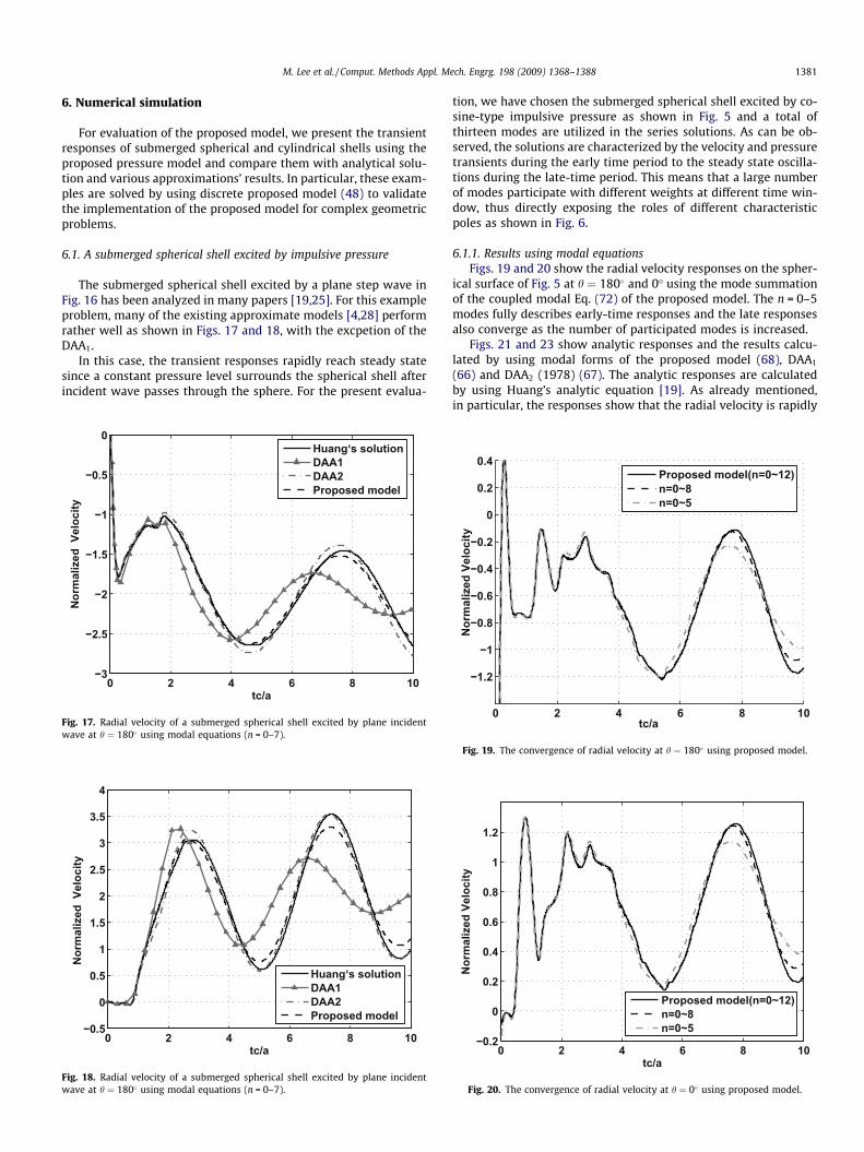
6. Numerical simulation

For evaluation of the proposed model, we present the transientresponses of submerged spherical and cylindrical shells using theproposed pressure model and compare them with analytical solu-tion and various approximations’ results. In particular, these exam-ples are solved by using discrete proposed model (48) to validatethe implementation of the proposed model for complex geometricproblems.

6.1. A submerged spherical shell excited by impulsive pressure

The submerged spherical shell excited by a plane step wave inFig. 16 has been analyzed in many papers [19,25]. For this exampleproblem, many of the existing approximate models [4,28] performrather well as shown in Figs. 17 and 18, with the excpetion of theDAA1.

In this case, the transient responses rapidly reach steady statesince a constant pressure level surrounds the spherical shell afterincident wave passes through the sphere. For the present evalua-

0 2 4 6 8 10−3

−2.5

−2

−1.5

−1

−0.5

0

tc/a

Nor

mal

ized

Vel

ocity

Huang‘s solutionDAA1DAA2Proposed model

Fig. 17. Radial velocity of a submerged spherical shell excited by plane incidentwave at h ¼ 180� using modal equations (n = 0–7).

0 2 4 6 8 10−0.5

0

0.5

1

1.5

2

2.5

3

3.5

4

tc/a

Nor

mal

ized

Vel

ocity

Huang‘s solutionDAA1DAA2Proposed model

Fig. 18. Radial velocity of a submerged spherical shell excited by plane incidentwave at h ¼ 180� using modal equations (n = 0–7).

tion, we have chosen the submerged spherical shell excited by co-sine-type impulsive pressure as shown in Fig. 5 and a total ofthirteen modes are utilized in the series solutions. As can be ob-served, the solutions are characterized by the velocity and pressuretransients during the early time period to the steady state oscilla-tions during the late-time period. This means that a large numberof modes participate with different weights at different time win-dow, thus directly exposing the roles of different characteristicpoles as shown in Fig. 6.

6.1.1. Results using modal equationsFigs. 19 and 20 show the radial velocity responses on the spher-

ical surface of Fig. 5 at h ¼ 180� and 0� using the mode summationof the coupled modal Eq. (72) of the proposed model. The n = 0–5modes fully describes early-time responses and the late responsesalso converge as the number of participated modes is increased.

Figs. 21 and 23 show analytic responses and the results calcu-lated by using modal forms of the proposed model (68), DAA1

(66) and DAA2 (1978) (67). The analytic responses are calculatedby using Huang’s analytic equation [19]. As already mentioned,in particular, the responses show that the radial velocity is rapidly

0 2 4 6 8 10

−1.2

−1

−0.8

−0.6

−0.4

−0.2

0

0.2

0.4N

orm

aliz

ed V

eloc

ity

tc/a

Proposed model(n=0~12)n=0~8n=0~5

Fig. 19. The convergence of radial velocity at h ¼ 180� using proposed model.

0 2 4 6 8 10−0.2

0

0.2

0.4

0.6

0.8

1

1.2

tc/a

Nor

mal

ized

Vel

ocity

Proposed model(n=0~12)n=0~8n=0~5

Fig. 20. The convergence of radial velocity at h ¼ 0� using proposed model.

1382 M. Lee et al. / Comput. Methods Appl. Mech. Engrg. 198 (2009) 1368–1388

changing at early time, and followed by the periodic oscillatory re-sponses. Observe that for the late-time period, the DAA2 (1978)and the proposed model follow with a reasonable phase and ampli-tude fidelity of the Huang’s radial velocity responses, but DAA1

shows large error in entire time range (see Figs. 22 and 24). TheDAA2 (1978), however, over(under)-estimates the early-time peakat / ¼ 180ð0Þ� while the proposed model predicts the early-timeresponses with high accuracy. This difference is caused by the inac-curacy of the low-mode impedance poles of the DAA2 (1978)shown in Fig. 6 and early-time inconsistency.

The early-time inconsistency manifests itself in impulse re-sponses function of the impedance. To this end, the cosine-typeimpulse velocities such as the cosine-type pressure to Eq. (72)were applied to initiate the pressure response. Figs. 25 and 26show the impulse pressure response and its error compared tothe analytic result at h ¼ 180�. Note that the two DAAs have largeerror at initial time due to the early-time inconsistency, whereasthe proposed model closely follow the analytical initial responsesince the present model is consistent with respect to the analyticinitial responses. The early-time consistency is an important char-

0 2 4 6 8 10−0.6

−0.4

−0.2

0

0.2

0.4

0.6

0.8

tc/a

Erro

r(Ve

loci

tyEx

act−V

eloc

ityEs

timat

ed)

DAA1DAA2Proposed model

Fig. 22. Error of radial velocity with respect to exact solution on a submergedspherical shell at h ¼ 180� using modal solution (n = 0–12).

0 2 4 6 8 10

−1.2

−1

−0.8

−0.6

−0.4

−0.2

0

0.2

0.4

0.6

0.8

tc/a

Nor

mal

ized

vel

ocity

Huang‘s solutionDAA1DAA2Proposed model

Fig. 21. Radial velocity at h ¼ 180� using modal solution (n = 0–12).

acteristic in pressure source identification or an array of acousticinverse problems.

Now, returning back in Fig. 5, that is, the frequency responses ofa spherical shell subjected to cosine-type impulse pressure is reex-amined. Figs. 27 and 28 show the frequency responses on the sur-face at h ¼ 180� and 0�. In these frequency responses, weintroduced structural loss factor [27], g by multiplying cs=c byð1þ ig=2Þ. Observe the DAA2 (1978) captures more accuratelythe low-frequency peaks of structural modes than the proposedmodel; however, the proposed model accurately estimates inter-mediate- and high-frequency peaks than the DAA2.

6.1.2. Responses using discrete boundary element equationsThe discrete boundary element models corresponding to DAA2

(1978) and proposed model, Eq. (48) were constructed. First, in or-der to validate the fidelity of the present discrete equation, thenumber of the boundary elements were increased from 385 to865. Fig. 29 shows the convergence of specific acoustic impedancepoles of discrete proposed model toward the those of the modalcorresponding theoretical model equation. As the number of ele-ment increases, the specific acoustic impedance poles of the pro-posed model using parameterized discrete matrix (47) approach

0 2 4 6 8 10

−0.6

−0.4

−0.2

0

0.2

0.4

0.6

tc/a

Erro

r(Ve

loci

tyEx

act−V

eloc

ityEs

timat

ed)

DAA1DAA2Proposed model

Fig. 24. Error of radial velocity with respect to exact solution on a submergedspherical shell at h ¼ 0� using modal solution (n = 0–12).

0 2 4 6 8 10

−0.4

−0.2

0

0.2

0.4

0.6

0.8

1

1.2

1.4

1.6

tc/a

Nor

mal

ized

Vel

ocity

Huang‘s solutionDAA1DAA2Proposed model

Fig. 23. Radial velocity at h ¼ 0� using modal solution (n = 0–12).

M. Lee et al. / Comput. Methods Appl. Mech. Engrg. 198 (2009) 1368–1388 1383

the specific acoustic impedance poles of modal equation (68) withthe weighting parameter, vn (69).

Now, in order to calculate transient responses, finite and bound-ary discrete element models in interaction Eq. (59) are constructedas 600 quad4 elements for both structure and acoustic equationand the coupled interaction Eq. (59) are solved by using the stag-gered solution [30] at each time step. In order to avoid discontinu-ity, we apply an impulsive pressure expressed in the form ofGaussian function as

pIð�t; hÞ ¼ cosh5ffiffiffiffipp exp½�52ð�t � 0:5Þ2�Hð�coshÞ; ð79Þ

HðxÞ ¼1 if x > 0;1=2 x ¼ 0;0 x < 0:

8><>: ð80Þ

‘Radial velocities using modal equation and the discrete models ofthe proposed model at h ¼ 180� and 0� are shown in Figs. 30 and31. The results calculated by the discrete models almost approachthe results by modal equation. Figs. 32 and 33 show the radialvelocities estimated by discrete models of various approximations.

0 1 2 3 4 5 6 7 8 9 10−1

−0.8

−0.6

−0.4

−0.2

0

0.2

0.4

0.6

0.8

1

tc/a

Nor

mal

ized

Pre

ssur

e

Huang‘s solutionDAA1DAA2Proposed model

Fig. 25. Impulse pressure responses of a spherical shell subjected to impulsevelocities at h ¼ 180� using modal solution (n = 0–12).

0 1 2 3 4 5 6 7 8 9 10−0.2

−0.15

−0.1

−0.05

0

0.05

0.1

0.15

0.2

Erro

r(Pr

essu

reEx

act−P

ress

ure Es

timat

ed) DAA1DAA2Proposed model

Fig. 26. Error of impulse pressure responses of a spherical shell subjected toimpulse velocities at h ¼ 180� using modal solution (n = 0–12).

We have included the result obtained by the fluid finite elementprovided by ANSYS commercial program [29] for which theabsorbing boundary [31] is used for this example problem. In mod-eling this problem by ANSYS code, the exterior acoustic domain upto 2R (two times of radius of a sphere) from the origin of a sphere ismodeled by the fluid volume elements. The elastic sphere and thefluid volume are treated as if they are a structure, and the absorb-ing boundary is modeled with 600 4-noded boundary elements.The responses calculated by the finite fluid elements and absorbingboundary show good early-time agreement and have a similartrend compared to the analytic results. But, the error betweenthe calculated results and analytic results increases in late-time re-sponses compared to those of the proposed model.

6.2. Application to an infinite cylindrical shell

The scattering pressure by a cylinder had been dealt with bymany previous researchers. Since Carrier [26] first derived themodal solution for an infinite submerged cylindrical shell interact-ing with exterior fluid, Mindlin and Bleich [1], Junger [32], Hay-wood [33] and other researchers have investigated the problem

0.5 1 1.5 2 2.5 3 3.5 4 4.5 5

10−1

100

101

|Rad

ial v

eloc

ity(ω

a/c)

|

ωa/c

Exact solutionDAA1DAA2Proposed model

Fig. 28. Frequency Response Function of radial velocity on a submerged sphericalshell with g ¼ 0:01 at h ¼ 0� (n = 0–12)

0.5 1 1.5 2 2.5 3 3.5 4 4.5 510−1

100

101|R

adia

l vel

ocity

(ωa/

c)|

ωa/c

Exact solutionDAA1DAA2Proposed model

Fig. 27. Frequency Response Function of radial velocity on a submerged sphericalshell with g ¼ 0:01 at h ¼ 180� (n = 0–12).

-6 -5 -4 -3 -2 -1 0-8

-6

-4

-2

0

2

4

6

8

Real

Imag

Modal solutionNumber of element : 385Number of element : 625Number of element : 865

-5 -4.5 -4 -3.5 -3 -2.5 -2-8

-7

-6

-5

-4

-3

-2

n=4

n=5

n=6

n=7

-6 -5 -4 -3 -2 -1 0-8

-6

-4

-2

0

2

4

6

8

Real

Imag

Modal solutionNumber of element : 385Number of element : 625Number of element : 865

-5 -4.5 -4 -3.5 -3 -2.5 -2-8

-7

-6

-5

-4

-3

-2

n=4

n=5

n=6

n=7

-5 -4.5 -4 -3.5 -3 -2.5 -2-8

-7

-6

-5

-4

-3

-2

n=4

n=5

n=6

n=7

Fig. 29. Convergence of specific acoustic impedance poles in discrete proposed model.

0 2 4 6 8 10−2.5

−2

−1.5

−1

−0.5

0

tc/a

Nor

mal

ized

Vel

ocity

Proposed(modal solution)Proposed(discrete mode)

Fig. 30. Radial velocity on a submerged spherical shell at h ¼ 180� using modalequation and discrete model of proposed model.

1384 M. Lee et al. / Comput. Methods Appl. Mech. Engrg. 198 (2009) 1368–1388

of an elastic infinite cylindrical shell excited by incident waves influid. Nevertheless, obtaining a rigorous solution remains a chal-lenge because the analytic inverse Laplace transform of a cylindri-cal wave equation dose not exist. Mindlin and Bleich [1] firstproposed the early-time approximation and Haywood [33] pre-sented the high-order approximation for solving the relation be-tween scattering pressure and velocity of a cylindrical wave.Huang [20] obtained modal solutions using contour integrate tech-nique and convolution integration to perform the inverse Laplacetransform of a cylindrical wave. Geers [34] also investigated themodal solution for an infinite cylindrical shell submerged in fluidusing residual potentials, but it is very complex.

In our correlation studies, we will use Huangs results [20] asaccurately traced as possible while recomputing the DAA2s results.In the modeling of an infinite long cylinder, we use a sufficientlylong cylindrical shell and to consider it to be an infinite cylinder.

6.2.1. A submerged infinite cylindrical shell subjected to plane wavesThe transient responses of an elastic cylindrical shell subjected

to a step plane wave have been obtained by Huang [20] and otherresearchers [34]. Huang obtained his analytic result within limitof series solution. In numerical methods, transient responses of asubmerged cylinder can be calculated by staggeringly solving inter-action equations, Eq. (59) in time sequence. We approximate a longcylindrical shell enough to consider it as an infinite cylindrical shellwith the length (L) to the radius (a) ratio to be 40. The cylinder hasthe following geometric and material parameters: m ¼ 0:3; L=a ¼40; hc=a ¼ 0:029 and qc=q ¼ 7:8 as shown in Fig. 34, and modeledthe long cylindrical shell and surrounding acoustic fluid by finiteelement and boundary element models, respectively. We firstexamine a long cylindrical shell subjected to incident step planewave such as adopted in Huang’s results [20]. The incident planewave’s pressure, pI and velocity, uI are defined in [34].

Fig. 35 shows the radial velocities on surface of a submergedcylindrical shell at h ¼ 180� and 0�. Here, the velocity response ath ¼ 0� is exactly zero until tc=a ¼ 1 because it takes tc=a � 1 forthe excitation by incident wave to arrive at h ¼ 0� through thecylindrical shell. But, since Huang’s result is obtained by finitemode summation, the velocity response at h ¼ 0 is not exactly zerofor 0 6 tc=a 6 1. The results calculated by the proposed model and

DAAs accurately approach Huang’s at early time with high accu-racy and also converge to Huang’s results at late time. At h ¼ 0 bothof proposed model and DAA2 show error at tc/a = 2, because of thediscontinuity of incident pressure at tc=a ¼ 2. Finally, in a cylindri-cal shell subjected to incident plane wave, the proposed model hasa similar performance to DAA2 because the responses rapidly gosteady state at early time. Therefore, all of approximations showgood accuracy.

6.2.2. A submerged infinite cylindrical shell subjected to cosine-typeimpulse pressure

In order to examine the transient dynamic responses of an infi-nite under-water cylindrical shell, we perform numerical simula-tion for same long cylinder subjected to cosine-type impulsepressure The cosine-type impulse pressure acting on the surfaceof a cylindrical shell is defined in the form of Gaussian function(79). The discrete pressure equation and the elastic structuralequations are the same ones generated in the previous section.

0

0.2

0.4

0.6

0.8

1

1.2

1.4

1.6

1.8

2

Nor

mal

ized

vel

ocity

Analytic resultDAA2Proposed modelFinite element & absorbing boundary

M. Lee et al. / Comput. Methods Appl. Mech. Engrg. 198 (2009) 1368–1388 1385

In order to evaluate the proposed model, we compared the re-sult of the proposed discrete boundary model with that of theDAAs’ and the domain based approximate model (Ansys) [29]’s re-sults. Fig. 36 shows the radial velocities on the surface of the cylin-drical shell at h ¼ 180� and 0�. Both the proposed model and theDAA2 show similar responses and the results of both models areclose to the results obtained by using the 2D ANSYS model.

We observe that the problem of a cylinder subjected to incidentpressure waves is essentially a two-dimensional problem. For thisparticular two-dimensional problem, little difference in responsesare noticed. While not comprehensive, we are tempted to concludethat various second-order models would yield adequate results,even perhaps the DAA1.

6.3. Shock analysis of a complex stiffened cylinder

So far the proposed approximate model is applied to simplestructures, a submerged sphere and an infinite cylinder. For suchproblems, the proposed model has been shown to yield accuratecoupled interaction responses. The fidelity of the present modelwill now be assessed by analyzing nontrivial problems, viz., shock

0 1 2 3 4 5 6 7 8 9 10−3.5

−3

−2.5

−2

−1.5

−1

−0.5

0

0.5

tc/a

Nor

mal

ized

vel

ocity

Analytic resultDAA2Proposed modelFinite element & absorbing boundary

Fig. 32. Radial velocity on a submerged spherical shell at h ¼ 180� using discretemodels.

0 2 4 6 8 10−0.2

0

0.2

0.4

0.6

0.8

1

1.2

1.4

tc/a

Nor

mal

ized

Vel

ocity

Proposed(modal solution)Proposed(discrete mode)

Fig. 31. Radial velocity on a submerged spherical shell at h ¼ 0� using modalequation and discrete model of proposed model.

analysis of complex stiffened cylinder subjected to a externalcharge. To this end, a steel ring-stiffened, circular cylinder of finitelength with flat aluminum end caps in [21] is analyzed as the thisstructure was a testbed of Defense Nuclear Agency (DNA) and the

ch

, ,c cE vρ

, in fluidcρ

O

Rv

θ

Q

P

w

na

Incident wave

Lch

, ,c cE vρ

, in fluidcρ

O

Rv

θ

Q

P

w

na

Incident wave

L

Fig. 34. A long cylindrical shell subjected to plane incident waves.

0 1 2 3 4 5−1.5

−1

−0.5

0

0.5

1

1.5

tc/a

Nor

mal

ized

vel

ocity

θ=180o

θ=0o

Huang’s resultDAA1(long cylinder)DAA2(long cylinder)Proposed(long cylinder)

Fig. 35. Radial velocity on the surface of an infinite cylindrical shell at h ¼ 180� and0�.

0 1 2 3 4 5 6 7 8 9 10−0.2

tc/a

Fig. 33. Radial velocity on a submerged spherical shell at h ¼ 0� using discretemodels.

θ

Shock wave

B A

D C θ

Fig. 38. Measured points on the surface.

1386 M. Lee et al. / Comput. Methods Appl. Mech. Engrg. 198 (2009) 1368–1388

Office of Naval Research (ONR) of USA for validating the DAA-basedcomputer code for predicting underwater explosion [21].

6.3.1. Computational model generationThe structure model is a ring-stiffened finite cylindrical shell

containing the internal structure and both flat ends consist of alu-minum caps. Dimensions of the model are taken from [35] and thematerial properties of steel and aluminum are chosen asE ¼ 2:9e7 psi;q ¼ 0:2836 lb=in3

; m ¼ 0:3 and E ¼ 9:858e6 psi;q ¼0:0975 lb=in3

; m ¼ 0:33. The finite element model of the steelring-stiffened, right circular cylinder consists of 5016 elementsand 17,616 degrees of freedom.

According to [21], in the experiment of underwater explosion,the side-on loading was produced by the underwater explosionof a 201.5 pound tapered charge of HBX-1 exploded at a stand-off distance of 69 feet. Both the model and the charge were sub-merged to a depth of 35 feet. The typical pressure–time historyfrom a pressure transducer located at about the stand-off distanceis reproduced from [21]. Fig. 37 shows the measured incident pres-sure from the pressure transducer and its simplified incident pres-sure for simulation.

0 1 2 3 4 5x 10−3

−100

−50

0

50

100

150

200

250

300

350

Time(sec)

Pres

sure

(psi

)

ExperimentSimulation

Fig. 37. Measured incident pressure and modified simple incident pressure locatedat about the stand-off distance.

0 1 2 3 4 5−1.8−1.6−1.4−1.2

−1−0.8−0.6−0.4−0.2

00.20.40.60.8

tc/a

Nor

mal

ized

vel

ocity

Finite element & absorbing boundary(2D)DAA1DAA2Proposed model

θ=0o

θ=180o

Fig. 36. Radial velocity on the surface of a long cylindrical shell subjected to cosine-type impulsive pressure at h ¼ 180� and h ¼ 0� .

6.3.2. Submerged shock analysisThe complex structure is surrounded by water whose density

and sound speed are q ¼ 0:0365 lb=in3; c ¼ 60000 in=s, respec-

tively. Therefore, exterior acoustic field strongly interacts withthe structural surface of the stiffened cylinder. As can be seen fromEq. (59), the structural finite element model and the exterior fluidboundary element model are coupled with each other and shockresponses by the incident wave shown in Fig. 37 can be also simu-lated. In reference paper, [21], each measured point is located asshown in Fig. 38.

0 0.5 1 1.5 2 2.5 3 3.5 4

x 10−3

−12

−10

−8

−6

−4

−2

0

2

4

6

8

10

Time(s)

Rad

ial V

elo

city

(ft/

s)

ExperimentDAA1DAA2Proposed model

Fig. 40. Radial velocity on the surface of a stiffened ring cylinder at B points (h ¼ 0�

and h ¼ 180�).

0 0.5 1 1.5 2 2.5 3 3.5 4

x 10−3

−10

−8

−6

−4

−2

0

2

4

6

8

10

12

Time(s)

No

rmal

vel

oci

ty(f

t/se

c)ExperimentDAA1DAA2Proposed model

Fig. 39. Radial velocity on the surface of a stiffened ring cylinder at A points (h ¼ 0�

and h ¼ 180�).

0 0.5 1 1.5 2 2.5 3 3.5 4

x 10−3

−20

−15

−10

−5

0

5

Time(s)

No

rmal

vel

oci

ty(f

t/se

c)

ExperimentDAA1DAA2Proposed model

Fig. 41. Radial velocity on the surface of a stiffened ring cylinder at C point.

0 0.5 1 1.5 2 2.5 3 3.5 4x 10−3

−12

−10

−8

−6

−4

−2

0

2

Time(s)

Rad

ial V

eloc

ity(ft

/s)

ExperimentDAA1DAA2Proposed model

Fig. 42. Radial velocity on the surface of a stiffened ring cylinder at D point.

M. Lee et al. / Comput. Methods Appl. Mech. Engrg. 198 (2009) 1368–1388 1387

Figs. 39 and 40 display the computed and experimental results.Point Aðh ¼ 0�Þ is the first contact point with the incoming incidentwave and all of the three approximations predict the early experi-mental peak response and experimental velocities satisfactorily. Atpoint B, approximate models overestimate the early time peak andthe error of estimation increases as the measured point is far awayfrom the midpoint of the model. This can be, perhaps, attributed todiscretization errors of the structure as well as incorrect materialproperties. Figs. 41 and 42 show normal velocities at the internallysupported structure. Although the normal velocities predicted bythe proposed approximate model cannot accurately capture theexperimental velocities, it shows similar trend with the experi-mental results. Hence, we conclude that the present approximateexternal acoustic model can be applied to acoustic–structure inter-action problems that are dominated by the structural responses,instead of acoustic propagation.

7. Conclusion

The present paper employs a weighted combination of the re-tarded and advanced potentials to derive a stable second-orderapproximate external acoustic model with a weighting parame-ter, v, for the case of continuum approximate model equation,

and a corresponding weighting matrix X for the discretized formof the model equation that is applicable for general interactionsurfaces.

The parametrization of the weighting parameter ðvÞ and thediscrete counter part (X) has been achieved by comparing themodal equation of the present model vs. the pole-zero character-istics of the analytical solution of an elastic sphere interactingwith external transient acoustic pressure fields. The present dis-crete pressure model (48) with the weighting matrix X may beviewed as a stabilized DAA2 with a curvature correction, withan added desirable early-time consistency for correctly capturingimpulse responses that may prove important for inverseproblems.

The performance of the proposed model have been assessed byapplying the present external acoustic model equation to vibrationand transient response analysis of several example problems. Tothis end, the analytical series solutions have been generated forstructures subjected to plain impulse incident acoustic pressure,cosine-type impulse incident pressure as well as plane step inci-dent wave. The same problems are solved by the present discretemodel pressure equation and the DAA2 equation. Comparisonsshow that the present model correctly capture initial impulse re-sponses whereas the DAA1 and DAA2 do not correctly capture theinitial impulse responses.

In order to further validate the present discrete model Eq. (48),eigenvalues of the coupled discrete acoustic–structural interactionequations employing the present discrete acoustic model and astandard finite element structural analyzer are compared withthose of the corresponding coupled modal equations for the spher-ical problem. Results show that, as the number of the discrete ele-ments increases, the coupled discrete eigenvalues approach tothose of the modal eigenvalues. A closer examination of thenumerical results conducted so far show that the DAA2 does tracesomewhat more accurately the late-time steady state responsesthan the present parameterized model equation when the coupledsteady state responses are dominated by structural rather thanacoustic contributions. On the other hand, the present parameter-ized pressure model equation exhibits substantially enhancedaccuracy for early-time responses that are desirable as a potentialcandidate model for system identification involving acoustic–structure interactions.

The present model has been assessed through a correlationstudy of a shock response experiment of a complex stiffened circu-lar cylinder. The simulation results follow experimental data rea-sonably faithfully both in terms of their pressure peaks and theirphases. Hence, the present discrete pressure model is recom-mended for use not only in transient simulations for arbitrarygeometries but also as a model equation for interaction systemidentification.

Nevertheless, we believe there is room for further improve-ments in capturing the highly oscillatory components in very flex-ible structures like balloons. This would call for a deeperunderstanding of the plane wave approximation used in the con-struction of the present model so that an improved correction ofthe present plane wave approximation may be needed. Such ave-nues are being actively studied.

Acknowledgement

This research was supported by National Research Laboratoryprogram through the Korea Science and Engineering Foundationfunded by the Ministry of Education, Science and Technology(R0A-2005-000-10112-0) and BK21. It is a pleasure to acknowl-edge the visiting appointment of K. C. Park that enabled the collab-orative work reported herein.

1388 M. Lee et al. / Comput. Methods Appl. Mech. Engrg. 198 (2009) 1368–1388

References

[1] R.D. Mindlin, H.H. Bleich, Response of an elastic cylindrical shell to atransverse, step shock wave, ASME J. Appl. Mech. 20 (1953) 189–195.

[2] P. Mann-Nachbar, The interaction of an acoustic wave and an elastic sphericalshell, Quart. Appl. Math. 15 (1) (1957) 83–93.

[3] M.C. Junger, Normal modes of submerged plates and shells, in: J.E. Greenspoon(Ed.), Fluid–Solid Interaction, ASME, NY, 1967.

[4] T.L. Geers, Doubly asymptotic approximation for transient motion ofsubmerged structures, J. Acoust. Soc. Am. 64 (1978) 1500–1508.

[5] C.A. Felippa, A family of early time approximations for fluid structureinteraction, ASME J. Appl. Mech. 47 (4) (1980) 703–708.

[6] T.L. Geers, C.A. Felippa, Doubly asymptotic approximations for vibration analysisof submerged structures, J. Acoust. Soc. Am. 173 (4) (1983) 1152–1159.

[7] R.J. Astley, Infinite elements for wave problems: a review of currentformulations and an assessment of accuracy, Int. J. Numer. Meth. Engrg. 49(7) (2000) 951–976.

[8] B.B. Baker, E.T. Copson, The Mathematical Theory of Huygens’s Principle,Clarendon Press, Oxford, 1949. pp. 23–45.

[9] J.A. Deruntz, The underwater shock analysis code and its applications, in:Shock and Vibration Symposium, Virginia Beach, VA, 1989.

[10] K.C. Park, Moonseok Lee, Youn-Sik Park, New approximations of externalacoustic–structural interactions, part I: model derivation, in: Proceedings ofThirteenth ICSV, Viena, Austria, 6 July, 2006.

[11] Moonseok Lee, Youn-Sik Park, K.C. Park, New approximations of externalacoustic–structural interactions, part II: model evaluation, in: Proceedings ofThirteenth ICSV, Viena, Austria, 6 July, 2006.

[12] Walter Ritz, Albert Einstein, Zum gegenw artigen Stand des Strahlungsproblems(on the current state of the radiation problem), Phys. Zeitschr. 10 (1909) 323–324.

[13] R.S. Fritzius, The Ritz–Einstein agreement to disagree, Phys. Essays 3 (1990)371–374.

[14] D.Z. Albert, Time and Chance, Harvard University Press, Cambridge, MA, 2000.[15] D.B. Malament, On the time reversal invariance of classical electromagnetic

theory, Stud. Hist. Philos. Modern Phys. 35 (2) (2004).[16] D.H. Chambers, A.K. Gautesen, Time reversal for a single spherical scatterer, J.

Acoust. Soc. Am. 109 (2001) 2616–2624.[17] M. Fink, Time reversal acoustics, Phys. Today 50 (1997) 34–40.[18] P.M. Morse, K.U. Ingard, Theoretical Acoustics, Priceton University Press, 1986.[19] H. Huang, Transient interaction of plane acoustic wave with a spherical elastic

shell, ASME J. Appl. Mech. 37 (1970) 1091–1099.

[20] H. Huang, An exact analysis of the transient interaction of acoustic planewaves with a cylindrical elastic shell, ASME J. Appl. Mech. 37 (1970) 1091–1099.

[21] Ranlet David, P. Raymond, Daddazio, A submerged shock response problemsuitable for use as a benchmark, in: The 68th Shock and Vibration Symposium,Hunt Valley, MD, 1997, pp. 3–7.(November).

[22] T.L. Geers, P. Zhang, Doubly asymptotic approximations for submergedstructures with internal fluid volumes: formulation, ASME J. Appl. Mech. 61(1994) 893–899.

[23] T.L. Geers, P. Zhang, Doubly asymptotic approximations for submergedstructures with internal fluid volumes: evaluation, ASME J. Appl. Mech. 61(1994) 900–906.

[24] J.A. DeRuntz, T.L. Geers, Added mass computation by the boundary integralmethod, Int. J. Num. Meth. Engrg. 12 (1977) 531–549.

[25] P. Zhang, T.L. Geers, Excitation of a fluid-filled, submerged spherical shell by atransient acoustic wave, J. Acoust. Soc. Am. 93 (1993) 696–705.

[26] G.F. Carrier, The interaction of an acoustic wave and an elastic cylindrical shell,Contract N7onr-35810, Technical Report No. 4 Brown University, Providence,RI, 1951.

[27] M.C. Junger, D. Feit, Sound Structure and their Interaction, second ed., MITPress, 1986.

[28] M.A. Sprague, T.L. Geers, Response of empty and fluid-filled, submergedspherical shells to plane and spherical, step-exponential acoustic waves, ShockVib. 6 (1999) 147–157.

[29] ANSYS, Inc., ANSYS Release Notes, Canonsburg, Release 11, USA, 2007.[30] K.C. Park, C.A. Felippa, J.A. DeRuntx, Stabilization of staggered solution

procedures for fluid–structure interaction analysis, ASME Computationalmethods for fluid–structure interaction problems AMD 26 (1977) 95–124(New York).

[31] L.F. Kallivokas, J. Bielak, R.C. MacCamy, Symmetric local absorbing boundariesin time and space, ASCE J. Engrg. Mech. 117 (9) (1991) 2027–2048.

[32] M.C. Junger, F.J. Rosato, The propagation of elastic waves in thin-walledcylindrical shells, J. Acoust. Soc. Am. 26 (1954) 709–713.

[33] J.H. Haywood, Response of an elastic cylindrical shell to a pressure pulse,Quart. Appl. Math. (XI) Part. 2 (1958) 129–141.

[34] T.L. Geers, Excitation of an elastic cylindrical shell by a transient acoustic wave,ASME J. Appl. Mech. 36 (1969) 459–469.

[35] D. Ranlet, F.L. Dimaggio, H.H. Bleigh, M.L. Baron, Elastic response of submergedshells with internally attached structure to shock loading, Comput. Struct. 7(1977) 355–364.