Computation of Margins to Power System Loadability Limits Using Phasor Measurement

Unit Data (or the SDG conjecture)

Peter W. Sauer University of Illinois at Urbana-Champaign

psauer@illinois.edu (In collaboration with Alejandro D. Dominguez-Garcia and two students – Jiangmeng Zhang, and Christian Sánchez)

April 6, 2012

TCIPG Seminar, Urbana, IL

Limits to Power System Operation (sources of congestion)

Thermal – short term and long term – typically measured in Amps or power (MW or MVA) – this one is fairly easy to find from measurements.

Voltage – plus or minus 5% of nominal – this one is fairly easy to find from measurements.

Stability – voltage collapse, SS stability, transient stability, bifurcations – margins to each critical point – this one is hard to find.

Other – Control limits - Ramp constraints, under/over excitation, taps – Short circuit current capability

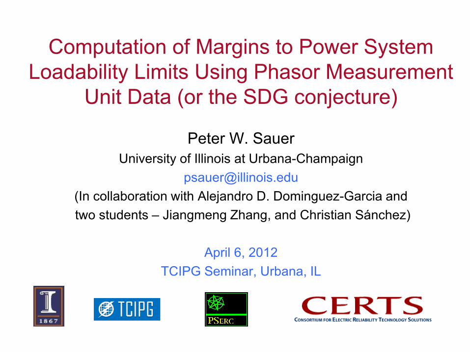
Limits to Power System Operation (sources of congestion)

Thermal – short term and long term – typically measured in Amps or power (MW or MVA) – this one is fairly easy to find from measurements.

Voltage – plus or minus 5% of nominal – this one is fairly easy to find from measurements.

Stability – voltage collapse, SS stability, transient stability, bifurcations – margins to each critical point – this one is hard to find.

Other – Control limits - Ramp constraints, under/over excitation, taps – Short circuit current capability

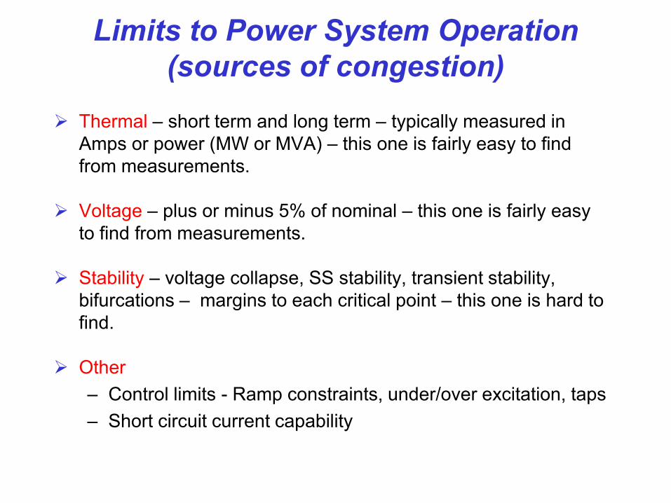
230 kV steel tower double circuit

Transmission Lines

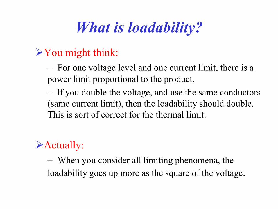
What is loadability? You might think:

– For one voltage level and one current limit, there is a power limit proportional to the product. – If you double the voltage, and use the same conductors (same current limit), then the loadability should double. This is sort of correct for the thermal limit.

Actually:

– When you consider all limiting phenomena, the loadability goes up more as the square of the voltage.

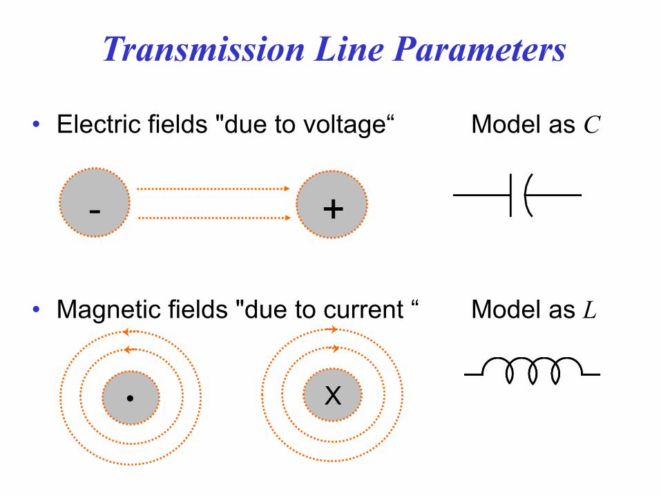
• Electric fields "due to voltage“ Model as C

• Magnetic fields "due to current “ Model as L

Transmission Line Parameters

+ -

X •

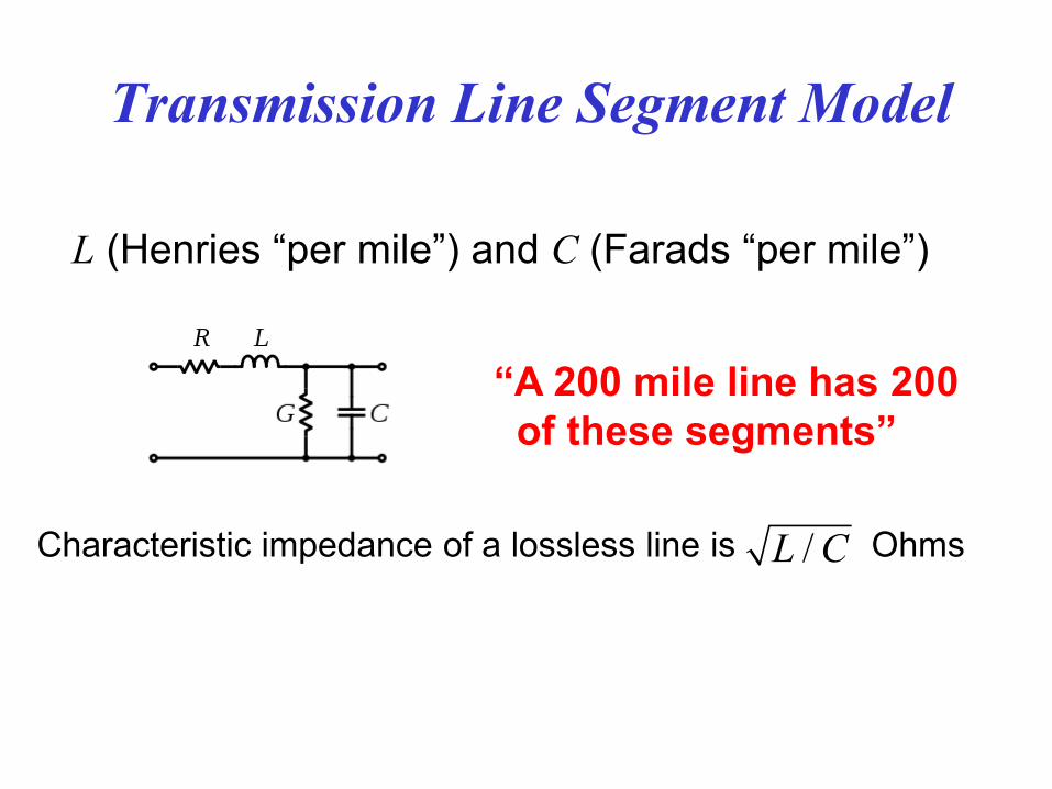
Transmission Line Segment Model

L (Henries “per mile”) and C (Farads “per mile”)

Characteristic impedance of a lossless line is Ohms /L C

“A 200 mile line has 200 of these segments”

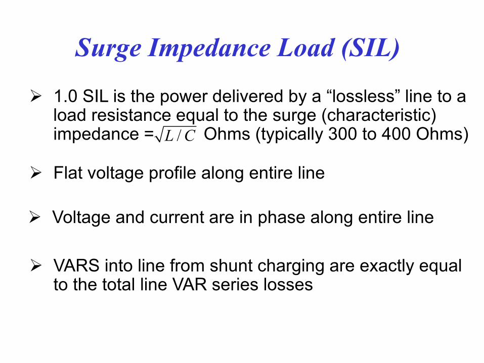
Surge Impedance Load (SIL)

1.0 SIL is the power delivered by a “lossless” line to a load resistance equal to the surge (characteristic) impedance = Ohms (typically 300 to 400 Ohms)

Voltage and current are in phase along entire line

VARS into line from shunt charging are exactly equal to the total line VAR series losses

Flat voltage profile along entire line

/L C

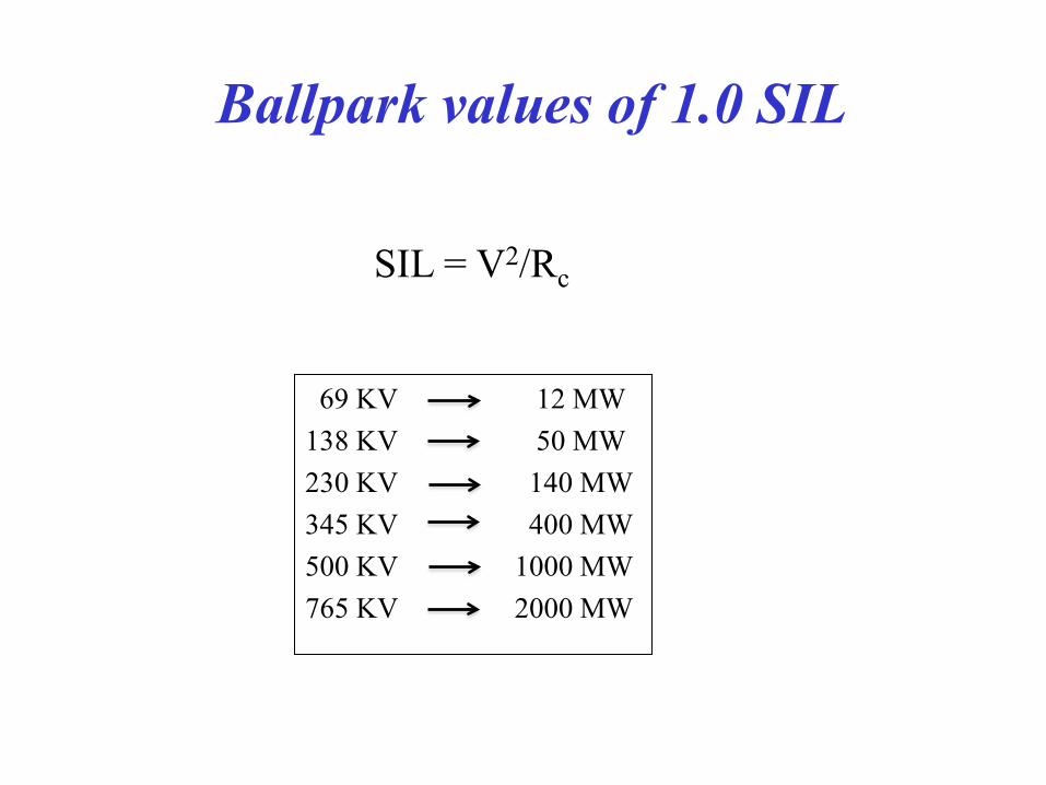
Ballpark values of 1.0 SIL

69 KV 12 MW 138 KV 50 MW 230 KV 140 MW 345 KV 400 MW 500 KV 1000 MW 765 KV 2000 MW

SIL = V2/Rc

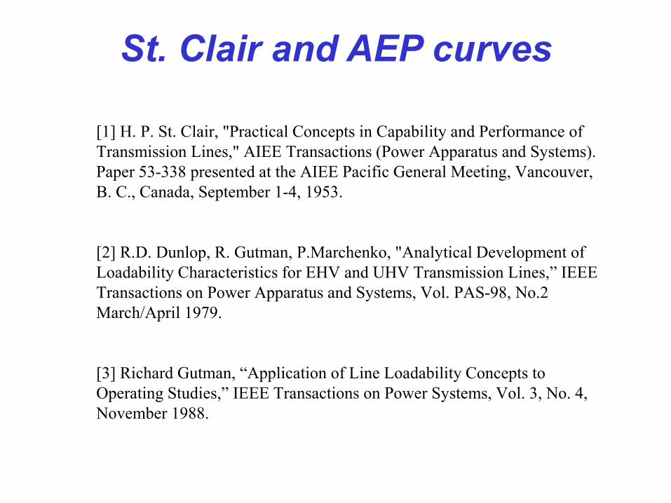
[1] H. P. St. Clair, "Practical Concepts in Capability and Performance of Transmission Lines," AIEE Transactions (Power Apparatus and Systems). Paper 53-338 presented at the AIEE Pacific General Meeting, Vancouver, B. C., Canada, September 1-4, 1953. [2] R.D. Dunlop, R. Gutman, P.Marchenko, "Analytical Development of Loadability Characteristics for EHV and UHV Transmission Lines,” IEEE Transactions on Power Apparatus and Systems, Vol. PAS-98, No.2 March/April 1979. [3] Richard Gutman, “Application of Line Loadability Concepts to Operating Studies,” IEEE Transactions on Power Systems, Vol. 3, No. 4, November 1988.

St. Clair and AEP curves

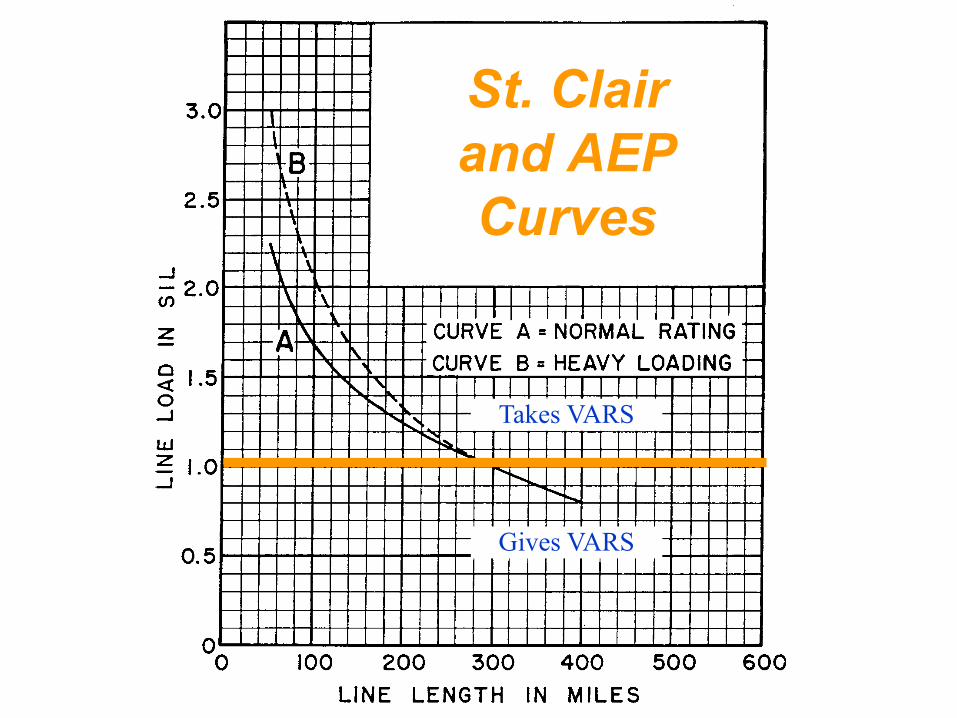
St. Clair and AEP Curves

Gives VARS

Takes VARS

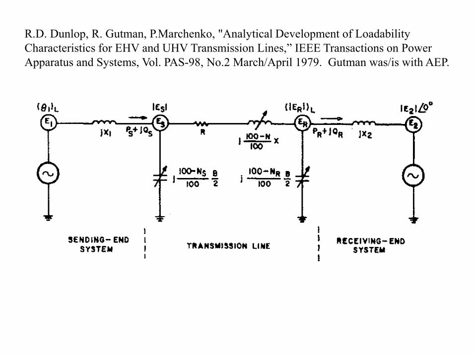
R.D. Dunlop, R. Gutman, P.Marchenko, "Analytical Development of Loadability Characteristics for EHV and UHV Transmission Lines,” IEEE Transactions on Power Apparatus and Systems, Vol. PAS-98, No.2 March/April 1979. Gutman was/is with AEP.

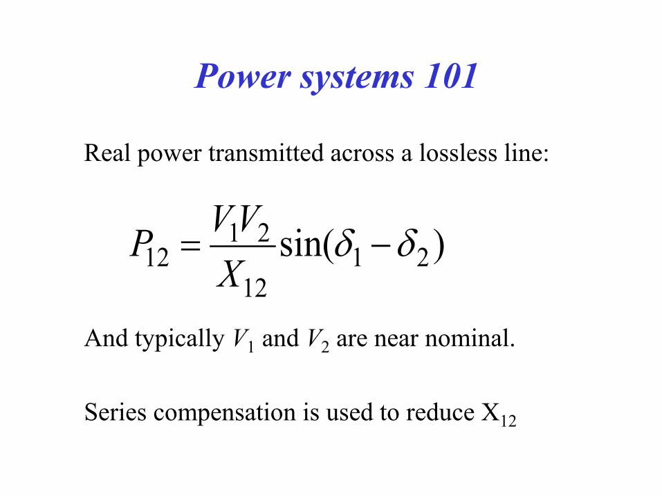
Power systems 101

Real power transmitted across a lossless line: And typically V1 and V2 are near nominal. Series compensation is used to reduce X12

1 212 1 2

12sin( )VVP

Xδ δ= −

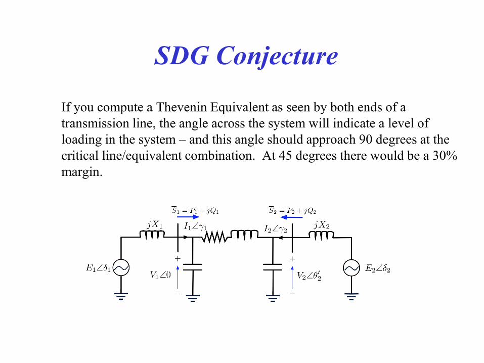
SDG Conjecture If you compute a Thevenin Equivalent as seen by both ends of a transmission line, the angle across the system will indicate a level of loading in the system – and this angle should approach 90 degrees at the critical line/equivalent combination. At 45 degrees there would be a 30% margin.

Others

St. Clair and AEP curves

T. He, S. Kolluri, S. Mandal, F. Galvan, P. Rastgoufard, “Identification of Weak Locations using Voltage Stability Margin Index”, APPLIED MATHEMATICS FOR RESTRUCTURED ELECTRIC POWER SYSTEMS – Optimization, Control, and Computational Intelligence, Edited by Joe H. Chow, Felix F. Wu, James A. Momoh, Springer, 2005, p. 25 -37. This was done for Entergy.

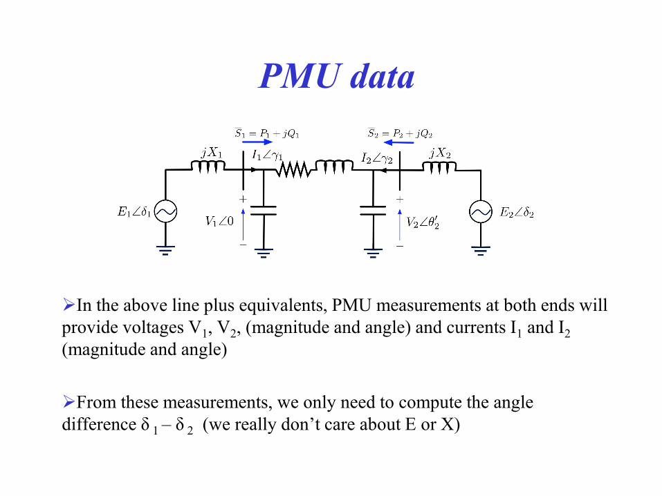
PMU data In the above line plus equivalents, PMU measurements at both ends will provide voltages V1, V2, (magnitude and angle) and currents I1 and I2 (magnitude and angle)

From these measurements, we only need to compute the angle difference δ 1 – δ 2 (we really don’t care about E or X)

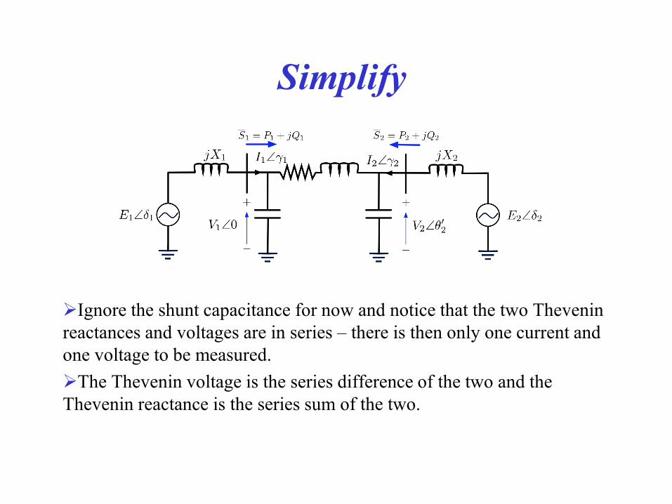
Simplify Ignore the shunt capacitance for now and notice that the two Thevenin reactances and voltages are in series – there is then only one current and one voltage to be measured. The Thevenin voltage is the series difference of the two and the Thevenin reactance is the series sum of the two.

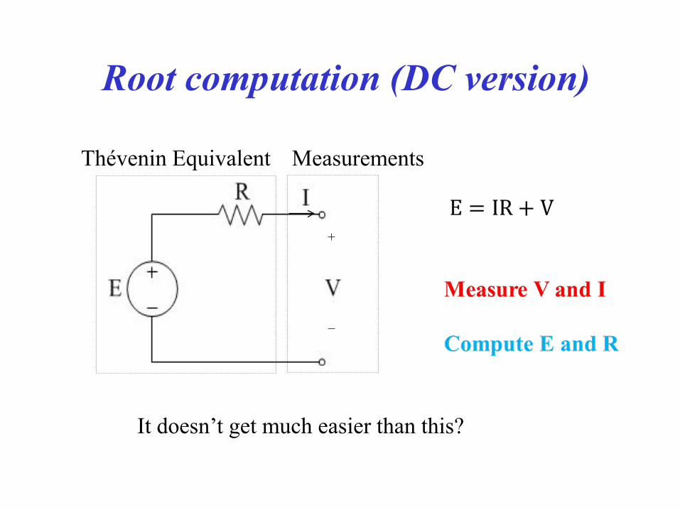
Root computation (DC version)

+

_

Thévenin Equivalent Measurements

It doesn’t get much easier than this?

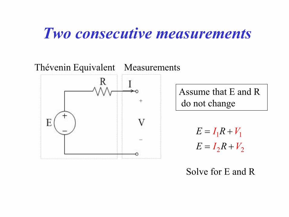
Two consecutive measurements

+

_ 1 1

2 2

E RE

IR

VI V

= += +

Assume that E and R do not change

Solve for E and R

Thévenin Equivalent Measurements

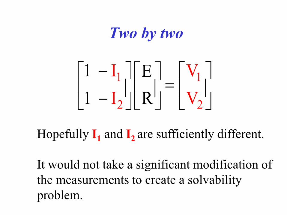
Two by two

1 1

2 2

1 E1 R

I VI V

− = −

Hopefully I1 and I2 are sufficiently different. It would not take a significant modification of the measurements to create a solvability problem.

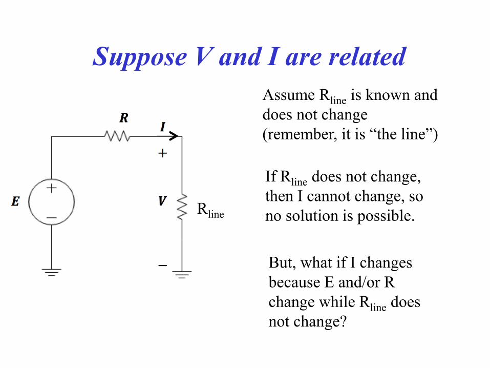
Suppose V and I are related

Assume Rline is known and does not change (remember, it is “the line”)

If Rline does not change, then I cannot change, so no solution is possible.

But, what if I changes because E and/or R change while Rline does not change?

Rline

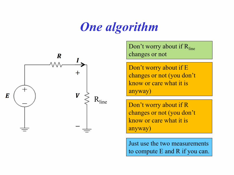
One algorithm

Don’t worry about if Rline changes or not

Don’t worry about if E changes or not (you don’t know or care what it is anyway)

Don’t worry about if R changes or not (you don’t know or care what it is anyway)

Just use the two measurements to compute E and R if you can.

Rline

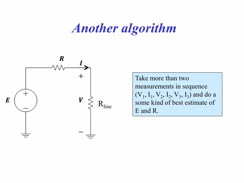
Another algorithm

Take more than two measurements in sequence (V1, I1, V2, I2, V3, I3) and do a some kind of best estimate of E and R.

Rline

The AC case

The measurements of line voltage V and current I are

complex numbers – fundamental frequency phasors.

The Thevenin equivalent has a complex E and Z.

Still a two-by-two problem, just with complex numbers.

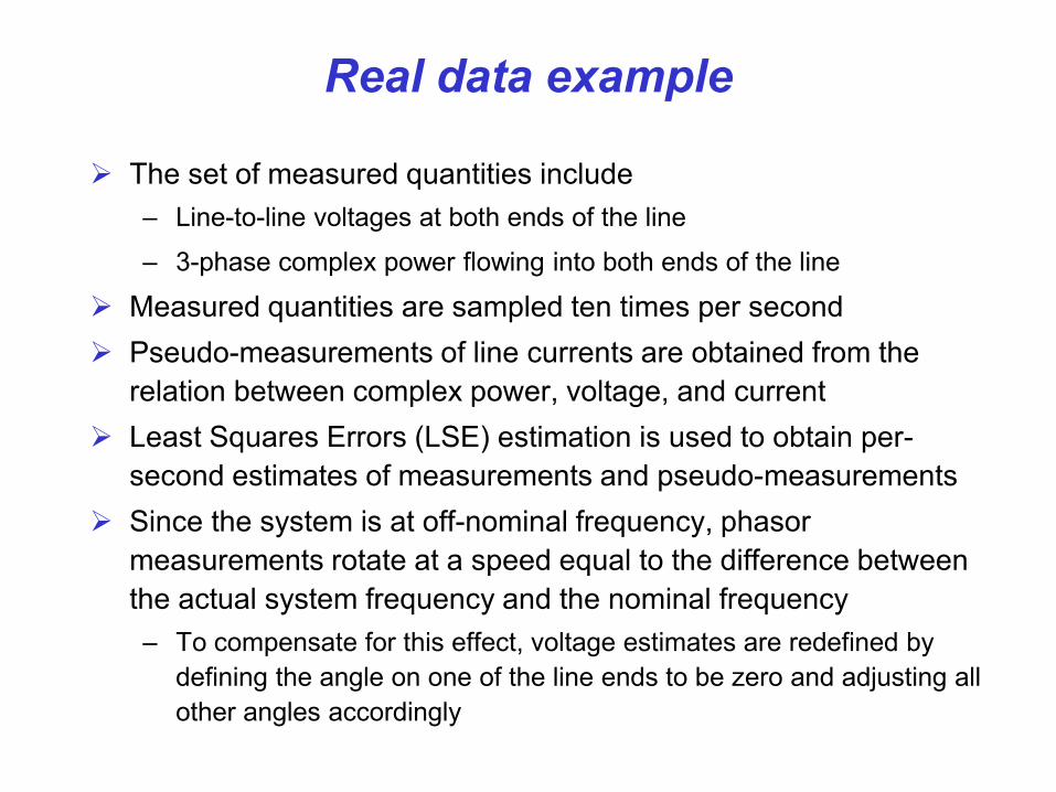
Real data example

The set of measured quantities include – Line-to-line voltages at both ends of the line

– 3-phase complex power flowing into both ends of the line Measured quantities are sampled ten times per second Pseudo-measurements of line currents are obtained from the

relation between complex power, voltage, and current Least Squares Errors (LSE) estimation is used to obtain per-

second estimates of measurements and pseudo-measurements Since the system is at off-nominal frequency, phasor

measurements rotate at a speed equal to the difference between the actual system frequency and the nominal frequency – To compensate for this effect, voltage estimates are redefined by

defining the angle on one of the line ends to be zero and adjusting all other angles accordingly

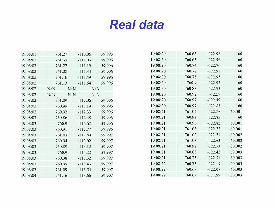
Real data

19:08:20 760.63 -122.96 60 19:08:20 760.63 -122.96 60 19:08:20 760.74 -122.96 60 19:08:20 760.78 -122.95 60 19:08:20 760.78 -122.95 60 19:08:20 760.9 -122.93 60 19:08:20 760.83 -122.93 60 19:08:20 760.92 -122.9 60 19:08:20 760.97 -122.89 60 19:08:20 760.97 -122.87 60 19:08:21 761.02 -122.86 60.001 19:08:21 760.93 -122.85 60 19:08:21 760.96 -122.82 60.001 19:08:21 761.03 -122.77 60.001 19:08:21 761.02 -122.71 60.002 19:08:21 761.03 -122.63 60.002 19:08:21 760.92 -122.53 60.002 19:08:21 760.83 -122.42 60.003 19:08:21 760.75 -122.31 60.003 19:08:22 760.73 -122.19 60.003 19:08:22 760.68 -122.08 60.003 19:08:22 760.69 -121.99 60.003

19:08:01 761.27 -110.86 59.995 19:08:02 761.33 -111.03 59.996 19:08:02 761.27 -111.19 59.996 19:08:02 761.28 -111.34 59.996 19:08:02 761.16 -111.49 59.996 19:08:02 761.13 -111.64 59.996 19:08:02 NaN NaN NaN 19:08:02 NaN NaN NaN 19:08:02 761.09 -112.06 59.996 19:08:02 760.99 -112.19 59.996 19:08:02 760.92 -112.33 59.996 19:08:03 760.86 -112.48 59.996 19:08:03 760.9 -112.62 59.996 19:08:03 760.91 -112.77 59.996 19:08:03 761.03 -112.89 59.997 19:08:03 760.94 -113.02 59.997 19:08:03 760.89 -113.12 59.997 19:08:03 760.9 -113.22 59.997 19:08:03 760.98 -113.32 59.997 19:08:03 760.99 -113.43 59.997 19:08:03 761.09 -113.54 59.997 19:08:04 761.16 -113.66 59.997

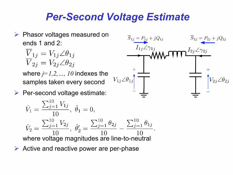
Per-Second Voltage Estimate

Per-second voltage estimate:

where voltage magnitudes are line-to-neutral Active and reactive power are per-phase

Phasor voltages measured on ends 1 and 2:

where j=1,2,…, 10 indexes the samples taken every second

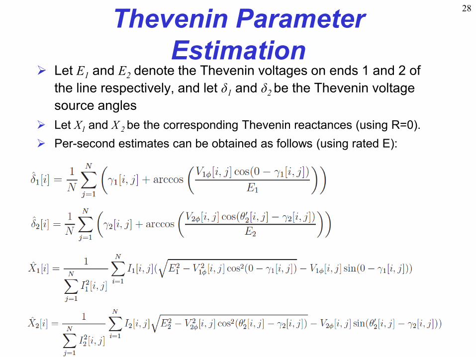
28 Thevenin Parameter Estimation

Let E1 and E2 denote the Thevenin voltages on ends 1 and 2 of the line respectively, and let δ1 and δ2 be the Thevenin voltage source angles

Let X1 and X 2 be the corresponding Thevenin reactances (using R=0). Per-second estimates can be obtained as follows (using rated E):

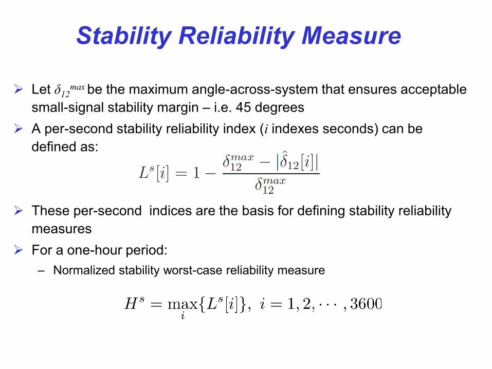
Stability Reliability Measure

Let δ12max be the maximum angle-across-system that ensures acceptable

small-signal stability margin – i.e. 45 degrees A per-second stability reliability index (i indexes seconds) can be

defined as:

These per-second indices are the basis for defining stability reliability measures

For a one-hour period: – Normalized stability worst-case reliability measure

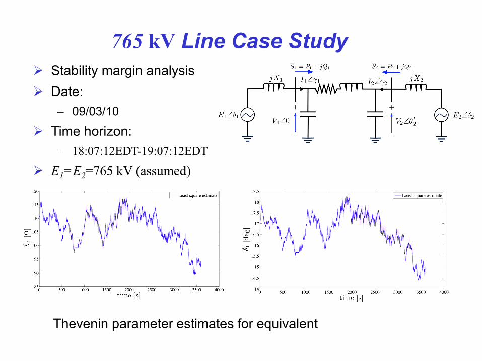
765 kV Line Case Study

Thevenin parameter estimates for equivalent

Stability margin analysis Date:

– 09/03/10

Time horizon: – 18:07:12EDT-19:07:12EDT

E1=E2=765 kV (assumed)

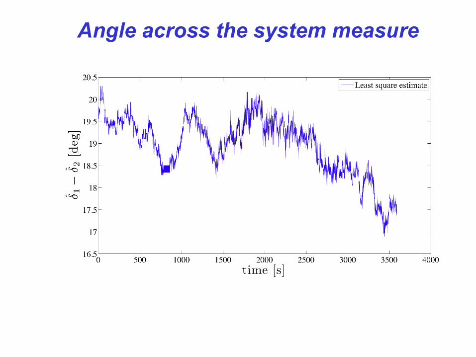
Angle across the system measure

Issues We know that the Thevenin equivalent changes between samples What does a “changing” equivalent mean in the math? How many samples do we need to have a well-conditioned problem? How can we decide if the problem is well-conditioned? Intrusion into the process could impact conditioning. What about contingencies (N-1)? Is the 45 degrees criteria correct? What is the “path” to the bifurcation? Is the “path” to the bifurcation important? How many lines need to be monitored? How do we verify this is correct? PMU data quality Can we push the computation down to the substation? A lot of this is really hard to prove because we do not know the answers!

Cyber threats

Spoofing of the Global Positioning System (GPS) would inject errors in PMU data and provide the wrong margin to maximum loadability – this is a TCIPG activity

Hacking into the data could result in ill-conditioned matrices that could not compute equivalents or operational limits – or erroneous equivalents that give the wrong margins.

Conclusions

PMU data offers the potential to perform operational reliability analysis without extensive model data.

There are technical issues yet to be clarified and shown. There are cyber security issues. Issue of contingencies needs to be included. PMU data quality needs to be assured. Tests for proper conditioning of data and matrices are needed