COMPUTATION OF MICROWAVE COMMUNICATION LINK …

International Multilingual Journal of Science and Technology (IMJST)

ISSN: 2528-9810

Vol. 5 Issue 6, June - 2020

www.imjst.org

IMJSTP29120290 1362

COMPUTATION OF MICROWAVE COMMUNICATION LINK OPTIMAL TRANSMISSION RANGE BASED ON EXTENDED STANFORD UNIVERSITY INTERIM PROPAGATION LOSS MODEL

Dike Happiness Ugochi

1

Department of Electrical/Electronic Engineering, Imo State

University (IMSU), Owerri, Nigeria

Corresponding Author: [email protected]

Isaac A. Ezenugu2

Department of Electrical/Electronic Engineering, Imo State

University (IMSU), Owerri, Nigeria

[email protected]

Abstract— In this paper, computation of microwave communication link optimal transmission range based on Extended Stanford University Interim (ESUI) propagation loss model is presented. The optimal transmission range is the path length at which the fade margin based on the propagation loss model is equal to the fade depth that can be encountered by the signal in the propagation path. Specifically, the mathematical expressions and modified fixed point numerical iteration algorithm for the computation of optimal transmission range of the microwave communication link is presented. Sample numerical example was presented using a dataset of a typical microwave communication link. The computation was carried out in Matlab software for the three different terrains specified in ESUI model. The microwave link site was in the ITU rain zone N with 95 mm/hr rain rate at 99.99% link availability. The results show that the microwave link in terrain A has the lowest optimal transmission range of 3.055648 km , the highest propagation loss of 150.6083 dB based on ESUI model, the lowest received signal strength of -70.6083 dB and the lowest effective fade margin of 11.39173 dB. On the other hand, the microwave link in terrain C has the highest optimal transmission range of 4.137131 km, the lowest propagation loss of 146.5764 dB based on ESUI model, the highest received signal strength of -66.57637 dB and the highest effective fade margin of 15.42363 dB. Essentially, comparison of the optimal transmission range and the propagation loss for the three different terrains shows that with the ESUI model, the terrain parameters have more impact on the propagation loss than the distance.

Keywords— Propagation Loss , Extended Stanford University Interim (ESUI) , Propagation Loss Model, Transmission Range, Optimal Transmission Range, Numerical Iteration

I. INTRODUCTION

The transmission range of wireless communication link

depends on a number of factors which include the

transmitter power, antenna gain, propagation loss, and other

network and environmental dependent factors [1, 2,

3,4,5,6,7]. Also, the dominant fade mechanism prevalent in

the signal propagation environment and applicable to the

given signal frequency also need to be considered

[8,9,10,11,12,13,14,15,16]. Communication link design is

meant to account for the listed factors so as to ensure

adequate quality of service is afforded within the network

coverage range.

In the line of sight (LoS) microwave communication link,

optimal transmission range indicates the link that has just

enough fade margin to accommodate the worst case fade

depth for the required percentage availability and bit error

rate [17,18, 19]. Accordingly, optimal transmission range

is in most cases smaller than the maximum possible

transmission range. The key criterion for the determination

of optimal transmission range is to determine the path

length at which the fade margin is equal to the fade depth.

In order to determine the fade margin, the link budget

equation is used to compute the received signal strength. At

this point, the propagation loss is required. Although in

many cases, the free space path loss is used. However,

researches have shown that free space path loss

underestimates the propagation loss as the transmission

range gets longer [20, 21, 22, 23]. As such, in this paper,

the Extended Stanford University Interim (ESUI)

propagation loss model is used in the link budget equation

to determine the received signal strength and by extension

the optimal transmission range of a microwave

communication link [24,25]. The determination of the

optimal transmission range requires iterative algorithm. As

such, a modified fixed point numerical iteration algorithm

[26, 27, 28, 29] was used in this paper to determine the

optimal path length. Sample microwave communication

link parameters dataset was used to demonstrate how the

ideas presented in this study can be applied.

II. METHODOLOGY

A. THE EXTENDED STANFORD UNIVERSITY INTERIM

(ESUI) MODEL

The Extended Stanford University Interim (ESUI) model is

a modified version of the Stanford University Interim (SUI)

propagation loss model [24,25]. The propagation loss

according to ESUI is given as 𝐿𝑃𝐸𝑋𝑆𝑈𝐼 where;

𝐿𝑃𝐸𝑋𝑆𝑈𝐼 =

{20 (log10 (

4𝜋𝑑

ʎ)) 𝑓𝑜𝑟 𝑑 < �́́�𝑜

𝐴 + 10𝛾 (log10 (𝑑

�́́�𝑜)) + 𝑋𝑓 + 𝑋ℎ 𝑓𝑜𝑟 𝑑 > �́́�𝑜

(1)

Where the d is distance in meters between the base station

and the mobile device, the frequency in MHz is denoted as

f, the reference distance, 𝑑0 = 100m , the modified

reference distance, �́́�𝑜 is given as;

http://www.imjst.org/


ISSN: 2528-9810


www.imjst.org

IMJSTP29120290 1363

�́́�𝑜 = 𝑑0 (10−(

𝑋ℎ−𝑋𝑓10(𝛾)

)) (2)

Also, the correction factor for receiving antenna height (in

meters) is 𝑋ℎ , the propagation loss exponent is 𝛾 , the

frequency correction factor is 𝑋𝑓 and the shadowing

correction factor is S where 8.2 ≤ S ≤ 10.6 dB and A is

given as:

𝐴 = 20 (log10 (4𝜋𝑑0

ʎ)) (3)

Also,

𝛾 = 𝑎 + 𝑏(ℎ𝑏) +𝑐

ℎ𝑏 (4)

Generally, for various terrains , the range of values for the

propagation loss exponent, 𝛾 are as follows:

{

γ = 2 for free space 3 < 𝛾 < 5 for urban environment

γ > 5 for indoor situations (5)

In addition, height in meters, hb for the base station antenna

is such that10 m ≤ hb ≤ 80 m. Again, for different terrain

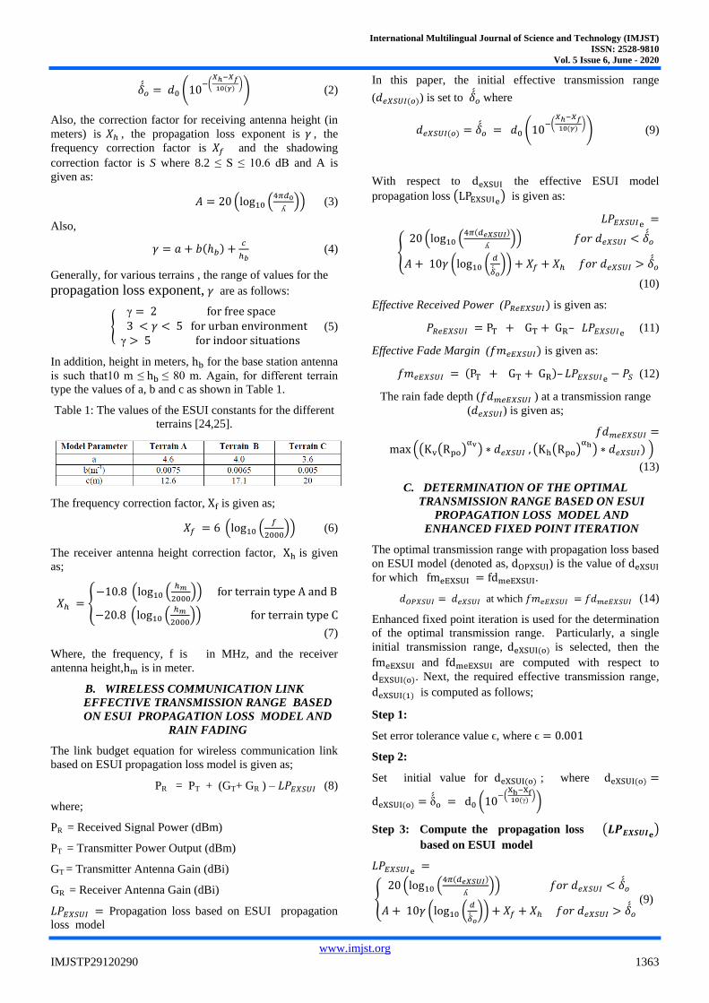
type the values of a, b and c as shown in Table 1.

Table 1: The values of the ESUI constants for the different

terrains [24,25].

The frequency correction factor, Xf is given as;

𝑋𝑓 = 6 (log10 (𝑓

2000)) (6)

The receiver antenna height correction factor, Xh is given

as;

𝑋ℎ = {−10.8 (log10 (

ℎ𝑚

2000)) for terrain type A and B

−20.8 (log10 (ℎ𝑚

2000)) for terrain type C

(7)

Where, the frequency, f is in MHz, and the receiver

antenna height,hm is in meter.

B. WIRELESS COMMUNICATION LINK

EFFECTIVE TRANSMISSION RANGE BASED

ON ESUI PROPAGATION LOSS MODEL AND

RAIN FADING

The link budget equation for wireless communication link

based on ESUI propagation loss model is given as;

PR = PT + (GT+ GR ) – 𝐿𝑃𝐸𝑋𝑆𝑈𝐼 (8)

where;

PR = Received Signal Power (dBm)

PT = Transmitter Power Output (dBm)

GT = Transmitter Antenna Gain (dBi)

GR = Receiver Antenna Gain (dBi)

𝐿𝑃𝐸𝑋𝑆𝑈𝐼 = Propagation loss based on ESUI propagation

loss model

In this paper, the initial effective transmission range

(𝑑𝑒𝑋𝑆𝑈𝐼(𝑜)) is set to �́́�𝑜 where

𝑑𝑒𝑋𝑆𝑈𝐼(𝑜) = �́́�𝑜 = 𝑑0 (10−(

𝑋ℎ−𝑋𝑓

10(𝛾))) (9)

With respect to deXSUI the effective ESUI model

propagation loss (LPEXSUIe) is given as:

𝐿𝑃𝐸𝑋𝑆𝑈𝐼e =

{20 (log10 (

4𝜋(𝑑𝑒𝑋𝑆𝑈𝐼)

ʎ)) 𝑓𝑜𝑟 𝑑𝑒𝑋𝑆𝑈𝐼 < �́́�𝑜

𝐴 + 10𝛾 (log10 (𝑑

�́́�𝑜)) + 𝑋𝑓 + 𝑋ℎ 𝑓𝑜𝑟 𝑑𝑒𝑋𝑆𝑈𝐼 > �́́�𝑜

(10)

Effective Received Power (𝑃𝑅𝑒𝐸𝑋𝑆𝑈𝐼) is given as:

𝑃𝑅𝑒𝐸𝑋𝑆𝑈𝐼 = PT + GT + GR– 𝐿𝑃𝐸𝑋𝑆𝑈𝐼e (11)

Effective Fade Margin (𝑓𝑚𝑒𝐸𝑋𝑆𝑈𝐼) is given as:

𝑓𝑚𝑒𝐸𝑋𝑆𝑈𝐼 = (PT + GT + GR)– 𝐿𝑃𝐸𝑋𝑆𝑈𝐼e− 𝑃𝑆 (12)

The rain fade depth (𝑓𝑑𝑚𝑒𝐸𝑋𝑆𝑈𝐼 ) at a transmission range

(𝑑𝑒𝑋𝑆𝑈𝐼) is given as;

𝑓𝑑𝑚𝑒𝐸𝑋𝑆𝑈𝐼 =

max ((Kv(Rpo)αv

) ∗ 𝑑𝑒𝑋𝑆𝑈𝐼 , (Kh(Rpo)αh) ∗ 𝑑𝑒𝑋𝑆𝑈𝐼) )

(13)

C. DETERMINATION OF THE OPTIMAL

TRANSMISSION RANGE BASED ON ESUI

PROPAGATION LOSS MODEL AND

ENHANCED FIXED POINT ITERATION

The optimal transmission range with propagation loss based

on ESUI model (denoted as, dOPXSUI) is the value of deXSUI

for which fmeEXSUI = fdmeEXSUI.

𝑑𝑂𝑃𝑋𝑆𝑈𝐼 = 𝑑𝑒𝑋𝑆𝑈𝐼 at which 𝑓𝑚𝑒𝐸𝑋𝑆𝑈𝐼 = 𝑓𝑑𝑚𝑒𝐸𝑋𝑆𝑈𝐼 (14)

Enhanced fixed point iteration is used for the determination

of the optimal transmission range. Particularly, a single

initial transmission range, deXSUI(o) is selected, then the

fmeEXSUI and fdmeEXSUI are computed with respect to

dEXSUI(o). Next, the required effective transmission range,

deXSUI(1) is computed as follows;

Step 1:

Set error tolerance value ϵ, where ϵ = 0.001

Step 2:

Set initial value for deXSUI(o) ; where deXSUI(o) =

deXSUI(o) = δ́́o = d0 (10−(

Xh−Xf10(γ)

))

Step 3: Compute the propagation loss (𝑳𝑷𝑬𝑿𝑺𝑼𝑰𝐞)

based on ESUI model

𝐿𝑃𝐸𝑋𝑆𝑈𝐼e =

{20 (log10 (

4𝜋(𝑑𝑒𝑋𝑆𝑈𝐼)

ʎ)) 𝑓𝑜𝑟 𝑑𝑒𝑋𝑆𝑈𝐼 < �́́�𝑜

𝐴 + 10𝛾 (log10 (𝑑

�́́�𝑜)) + 𝑋𝑓 + 𝑋ℎ 𝑓𝑜𝑟 𝑑𝑒𝑋𝑆𝑈𝐼 > �́́�𝑜

(9)



ISSN: 2528-9810


www.imjst.org

IMJSTP29120290 1364

Step 4: Compute the effective fade margin (𝐟𝐦𝐞𝐄𝐗𝐒𝐔𝐈)

𝑓𝑚𝑒𝐸𝑋𝑆𝑈𝐼 = (PT + GT + GR)– 𝐿𝑃𝐸𝑋𝑆𝑈𝐼e− 𝑃𝑆

Step 5: Compute the rain fade depth, 𝑓𝑑𝑚𝑒𝐸𝑋𝑆𝑈𝐼 =

𝑓𝑑𝑚𝑒𝐸𝑋𝑆𝑈𝐼 =

max ((Kv(Rpo)αv

) ∗ 𝑑𝑒𝑋𝑆𝑈𝐼 , (Kh(Rpo)αh) ∗ 𝑑𝑒𝑋𝑆𝑈𝐼) )

Step 6: Check if optimal transmission range has been

obtained

If |𝑓𝑚𝑒𝐸𝑋𝑆𝑈𝐼 − 𝑓𝑑𝑚𝑒𝐸𝑋𝑆𝑈𝐼| < |𝜖| Then

𝑑𝑂𝑃𝑋𝑆𝑈𝐼 = 𝑑𝑒𝑋𝑆𝑈𝐼(𝑜)

“Output Optimal transmission range , dOPXSUI =”

, deXSUI(o)

Goto step 10

Endif

Step 7: Compute the next transmission range

IF 𝑓𝑚𝑒𝐸𝑋𝑆𝑈𝐼 > 𝑓𝑑𝑚𝑒𝐸𝑋𝑆𝑈𝐼

Δ𝐹𝑒𝑋 =𝑓𝑚𝑒𝐸𝑋𝑆𝑈𝐼 - 𝑓𝑑𝑚𝑒𝐸𝑋𝑆𝑈𝐼

deX =(fdmeEXSUI

ΔFeX ) dEXSUI(o)

𝑑𝐸𝑋𝑆𝑈𝐼(1) = 𝑑𝐸𝑋𝑆𝑈𝐼(𝑜) + 𝑑𝑒𝑋 = 𝑑𝐸𝑋𝑆𝑈𝐼(𝑜) (1 +

(𝑓𝑑𝑚𝑒𝐸𝑋𝑆𝑈𝐼

Δ𝐹𝑒𝑋 ))

𝐸𝑠𝑙𝑒IF 𝑓𝑚𝑒𝐸𝑋𝑆𝑈𝐼 < 𝑓𝑑𝑚𝑒𝐸𝑋𝑆𝑈𝐼

ΔFeX = fdmeEXSUI − fmeEXSUI

𝑑𝑒𝑋 =(𝑓𝑚𝑒𝐸𝑋𝑆𝑈𝐼

Δ𝐹𝑒𝑋 ) 𝑑𝐸𝑋𝑆𝑈𝐼(𝑜)

𝑑𝐸𝑋𝑆𝑈𝐼(1) = 𝑑𝐸𝑋𝑆𝑈𝐼(𝑜) - 𝑑𝑒𝑋 = 𝑑𝐸𝑋𝑆𝑈𝐼(𝑜) (1 −

(𝑓𝑚𝑒𝐸𝑋𝑆𝑈𝐼

Δ𝐹𝑒𝑋 ))

End if

Step 8 : Reset the guess optimal path length

𝑑𝐸𝑋𝑆𝑈𝐼(0) =𝑑𝐸𝑋𝑆𝑈𝐼(1)

Step 9 : Repeat the steps from step 3

Goto step 3

Step 10 End the program

Stop

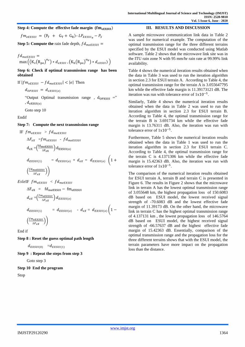
III. RESULTS AND DISCUSSION

A sample microwave communication link data in Table 2

was used for numerical example. The computation of the

optimal transmission range for the three different terrains

specified by the ESUI model was conducted using Matlab

software. Table 2 shows that the microwave link site was in

the ITU rain zone N with 95 mm/hr rain rate at 99.99% link

availability.

Table 4 shows the numerical iteration results obtained when

the data in Table 3 was used to run the iteration algorithm

in section 2.3 for ESUI terrain A. According to Table 4, the

optimal transmission range for the terrain A is 3.055647795

km while the effective fade margin is 11.39173121 dB. The

iteration was run with tolerance error of 1x10−5.

Similarly, Table 4 shows the numerical iteration results

obtained when the data in Table 2 was used to run the

iteration algorithm in section 2.3 for ESUI terrain B.

According to Table 4, the optimal transmission range for

the terrain B is 3.691734 km while the effective fade

margin is 13.76311 dB. Also, the iteration was run with

tolerance error of 1x10−5.

Furthermore, Table 5 shows the numerical iteration results

obtained when the data in Table 1 was used to run the

iteration algorithm in section 2.3 for ESUI terrain C.

According to Table 4, the optimal transmission range for

the terrain C is 4.1371306 km while the effective fade

margin is 15.42363 dB. Also, the iteration was run with

tolerance error of 1x10−5.

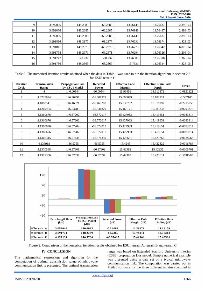
The comparison of the numerical iteration results obtained

for ESUI terrain A, terrain B and terrain C is presented in

Figure 6. The results in Figure 2 shows that the microwave

link in terrain A has the lowest optimal transmission range

of 3.055648 km, the highest propagation loss of 150.6083

dB based on ESUI model, the lowest received signal

strength of -70.6083 dB and the lowest effective fade

margin of 11.39173 dB. On the other hand, the microwave

link in terrain C has the highest optimal transmission range

of 4.137131 km , the lowest propagation loss of 146.5764

dB based on ESUI model, the highest received signal

strength of -66.57637 dB and the highest effective fade

margin of 15.42363 dB. Essentially, comparison of the

optimal transmission range and the propagation loss for the

three different terrains shows that with the ESUI model, the

terrain parameters have more impact on the propagation

loss than the distance.



ISSN: 2528-9810


www.imjst.org

IMJSTP29120290 1365

Table 2: A sample microwave communication link data used for the numerical iteration of optimal for the three terrains

specified in ESUI

Table 3: The numerical iteration results obtained when the data in Table 1 was used to run the iteration algorithm in section

2.3 for ESUI terrain A

Iteration Cycle Transmission

Range

Propagation Loss

by ESUI Model Received Power

Effective Fade

Margin

Effective Rain

Fade Depth Error

1 4.000000000 156.0058203 -76.00582035 5.994179653 14.9123783 8.92E+00

2 3.401960004 152.7600545 -72.76005448 9.239945518 12.6828287 3.44E+00

3 3.102940005 150.9160932 -70.91609317 11.08390683 11.5680538 4.84E-01

4 3.102940005 150.9160932 -70.91609317 11.08390683 11.5680538 4.84E-01

5 3.102940005 150.9160932 -70.91609317 11.08390683 11.5680538 4.84E-01

6 3.065562506 150.6731964 -70.67319635 11.32680365 11.428707 1.02E-01

7 3.065562506 150.6731964 -70.67319635 11.32680365 11.428707 1.02E-01

8 3.056218131 150.6120094 -70.6120094 11.3879906 11.3938703 5.88E-03

9 3.056218131 150.6120094 -70.6120094 11.3879906 11.3938703 5.88E-03

10 3.056218131 150.6120094 -70.6120094 11.3879906 11.3938703 5.88E-03

11 3.056218131 150.6120094 -70.6120094 11.3879906 11.3938703 5.88E-03

12 3.056218131 150.6120094 -70.6120094 11.3879906 11.3938703 5.88E-03

13 3.055926119 150.6100943 -70.61009429 11.38990571 11.3927816 2.88E-03

14 3.055780113 150.6091367 -70.60913667 11.39086333 11.3922373 1.37E-03

15 3.05570711 150.6086578 -70.60865784 11.39134216 11.3919651 6.23E-04

16 3.055670609 150.6084184 -70.60841842 11.39158158 11.3918291 2.47E-04

17 3.055652358 150.6082987 -70.60829871 11.39170129 11.391761 5.97E-05

18 3.055652358 150.6082987 -70.60829871 11.39170129 11.391761 5.97E-05

19 3.055647795 150.6082688 -70.60826879 11.39173121 11.391744 1.28E-05

20 3.055647795 150.6082688 -70.60826879 11.39173121 11.391744 1.28E-05

Table 4: The numerical iteration results obtained when the data in Table 1 was used to run the iteration algorithm in section

2.3 for ESUI terrain B

Iteration Cycle Transmission

Range Propagation Loss

by ESUI Model

Received

Power

Effective Fade

Margin

Effective Rain

Fade Depth Error

1 4 149.6884 -69.6884 12.31158 14.91238 2.60E+00

2 3.825595 148.8815 -68.8815 13.11845 14.26218 1.14E+00

3 3.738392 148.4642 -68.4642 13.53579 13.93708 4.01E-01

4 3.694791 148.2519 -68.2519 13.74813 13.77453 2.64E-02

5 3.694791 148.2519 -68.2519 13.74813 13.77453 2.64E-02

6 3.694791 148.2519 -68.2519 13.74813 13.77453 2.64E-02

7 3.694791 148.2519 -68.2519 13.74813 13.77453 2.64E-02

8 3.692066 148.2385 -68.2385 13.76148 13.76437 2.89E-03



ISSN: 2528-9810


www.imjst.org

IMJSTP29120290 1366

9 3.692066 148.2385 -68.2385 13.76148 13.76437 2.89E-03

10 3.692066 148.2385 -68.2385 13.76148 13.76437 2.89E-03

11 3.692066 148.2385 -68.2385 13.76148 13.76437 2.89E-03

12 3.691896 148.2377 -68.2377 13.76231 13.76374 1.42E-03

13 3.691811 148.2373 -68.2373 13.76273 13.76342 6.87E-04

14 3.691768 148.2371 -68.2371 13.76294 13.76326 3.20E-04

15 3.691747 148.237 -68.237 13.76305 13.76318 1.36E-04

16 3.691736 148.2369 -68.2369 13.7631 13.76314 4.42E-05

Table 5 The numerical iteration results obtained when the data in Table 1 was used to run the iteration algorithm in section 2.3

for ESUI terrain C

Iteration

Cycle

Transmission

Range

Propagation Loss

by ESUI Model

Received

Power

Effective Fade

Margin

Effective Rain Fade

Depth Error

1 4 146.00544 -66.00544 15.99456 14.912378 -1.0821821

2 4.0725694 146.30997 -66.309971 15.690029 15.182924 -0.507105

3 4.1088541 146.46021 -66.460208 15.539792 15.318197 -0.2215955

4 4.1269964 146.53483 -66.534829 15.465171 15.385833 -0.0793375

5 4.1360676 146.57202 -66.572017 15.427983 15.419651 -0.0083314

6 4.1360676 146.57202 -66.572017 15.427983 15.419651 -0.0083314

7 4.1360676 146.57202 -66.572017 15.427983 15.419651 -0.0083314

8 4.1360676 146.57202 -66.572017 15.427983 15.419651 -0.0083314

9 4.1366345 146.57434 -66.574339 15.425661 15.421765 -0.0038963

10 4.136918 146.5755 -66.5755 15.4245 15.422822 -0.0016788

11 4.1370598 146.57608 -66.57608 15.42392 15.42335 -0.0005701

12 4.1371306 146.57637 -66.57637 15.42363 15.423614 -1.574E-05

Figure 2. Comparison of the numerical iteration results obtained for ESUI terrain A, terrain B and terrain C

IV. CONCLUSION

The mathematical expressions and algorithm for the

computation of optimal transmission range of microwave

communication link is presented. The optimal transmission

range was based on Extended Stanford University Interim

(ESUI) propagation loss model. Sample numerical example

was presented using a data set of a typical microwave

communication link. The computation was carried out in

Matlab software for the three different terrains specified in

Path Length Rain(km)

Propagation Lossby ESUI Model

(dB)

Received Power(dB)

Effective FadeMargin (dB)

Effective RainFading (dB)

Terrain A 3.055648 150.6083 -70.6083 11.39173 11.39174

Terrain B 3.691734 148.2369 -68.2369 13.76311 13.76313

Terrain C 4.137131 146.5764 -66.57637 15.42363 15.42361

-80

-30

20

70

120



ISSN: 2528-9810


www.imjst.org

IMJSTP29120290 1367

ESUI model. The results show that with ESUI model, the

terrain parameters have more impact on the value of the

propagation loss than the distance. As such, the ESUi

terrain A presented the highest propagation loss and the

lowest transmission range.

REFERENCES

1. Akaninyene B. Obot , Ozuomba Simeon and

Afolanya J. Jimoh (2011); “Comparative Analysis

Of Pathloss Prediction Models For Urban

Macrocellular” Nigerian Journal of Technology

(NIJOTECH) Vol. 30, No. 3 , October 2011 , PP

50 – 59

2. Habib, A., & Moh, S. (2019). Wireless channel

models for over-the-sea communication: A

comparative study. Applied Sciences, 9(3), 443.

3. Njoku Chukwudi Aloziem, Ozuomba Simeon,

Afolayan J. Jimoh (2017) Tuning and Cross

Validation of Blomquist-Ladell Model for Pathloss

Prediction in the GSM 900 Mhz Frequency Band ,

International Journal of Theoretical and Applied

Mathematics, Journal: Environmental and Energy

Economics

4. Habib, A., & Moh, S. (2018, December). A Survey

on Channel Models for Radio Propagation over the

Sea Surface. In Proceedings of the 10th International

Conference on Internet (ICONI 2018), Phnom Penh,

Cambodia (pp. 1-3).

5. Ozuomba, S., Enyenihi, J., & Rosemary, N. C.

(2018). Characterisation of Propagation Loss for a

3G Cellular Network in a Crowded Market Area

Using CCIR Model. Review of Computer

Engineering Research, 5(2), 49-56.

6. Ozuomba, S., Johnson, E. H., & Udoiwod, E. N.

(2018). Application of Weissberger Model for

Characterizing the Propagation Loss in a Gliricidia

sepium Arboretum. Universal Journal of

Communications and Network 6(2): 18-23, 2018

7. Ozuomba, Simeon (2019) EVALUATION OF

OPTIMAL TRANSMISSION RANGE OF

WIRELESS SIGNAL ON DIFFERENT TERRAINS

BASED ON ERICSSON PATH LOSS MODEL ,

Science and Technology Publishing (SCI & TECH)

8. Khan, N. M. (2006). Modeling and characterization

of multipath fading channels in cellular mobile

communication systems. University of New South

Wales.

9. Rudd, R., Craig, K., Ganley, M., & Hartless, R.

(2014). Building materials and propagation. Final

Report, Ofcom, 2604.

10. Ononiwu, G., Ozuomba, S., & Kalu, C. (2015).

Determination of the dominant fading and the

effective fading for the rain zones in the ITU-R P.

838-3 recommendation. European Journal of

Mathematics and Computer Science Vol, 2(2).

11. Rappaport, T. S., MacCartney, G. R., Sun, S., Yan,

H., & Deng, S. (2017). Small-scale, local area, and

transitional millimeter wave propagation for 5G

communications. IEEE Transactions on Antennas

and Propagation, 65(12), 6474-6490.

12. Kalu, C., Ozuomba, S. & Jonathan, O. A. (2015).

Rain rate trend-line estimation models and web

application for the global ITU rain zones. European

Journal of Engineering and Technology, 3 (9), 14-29

13. Cotton, S. L., D'Errico, R., & Oestges, C. (2014). A

review of radio channel models for body centric

communications. Radio Science, 49(6), 371-388.

14. Akaninyene B. Obot , Ozuomba Simeon and

Kingsley M. Udofia (2011); “Determination Of

Mobile Radio Link Parameters Using The Path Loss

Models” NSE Technical Transactions , A Technical

Journal of The Nigerian Society Of Engineers, Vol.

46, No. 2 , April - June 2011 , PP 56 – 66.

15. Ajayi, T. S. (2007). Mobile Satellite

Communications: Channel Characterization and

Simulation.

16. Ozuomba, Simeon, Constance Kalu, and Akaninyene

B. Obot. (2016) "Comparative Analysis of the ITU

Multipath Fade Depth Models for Microwave Link

Design in the C, Ku, and Ka-Bands." Mathematical

and Software Engineering 2.1 (2016): 1-8.

17. Ozuomba Simeon, Henry Akpan Jacob and Kalu

Constance ( 2019) Analysis Of Single Knife Edge

Diffraction Loss For A Fixed Terrestrial Line-Of-

Sight Microwave Communication Link Journal of

Multidisciplinary Engineering Science and

Technology (JMEST)

18. Kalu, C. (2019). Development and Performance

Analysis of Bisection Method-Based Optimal Path

Length Algorithm for Terrestrial Microwave

Link. Review of Computer Engineering

Research, 6(1), 1-11.

19. Johnson, E. H., Ozuomba, S., & Asuquo, I. O.

(2019). Determination of Wireless Communication

Links Optimal Transmission Range Using Improved

Bisection Algorithm. Universal Journal of

Communications and Network 7(1): 9-20, 2019

20. Plets, D., Mangelschots, R., Vanhecke, K., Martens,

L., & Joseph, W. (2016, September). A mobile app

for real-time testing of path-loss models and

optimization of network planning. In 2016 IEEE

27th Annual International Symposium on Personal,

Indoor, and Mobile Radio Communications

(PIMRC) (pp. 1-7). IEEE.

21. Series, P. (2015). Propagation data and prediction

methods for the planning of short-range outdoor

radiocommunication systems and radio local area

networks in the frequency range 300 MHz to 100

GHz. tech. rep., ITU, Tech. Rep. ITU-R.

22. Mauwa, H., Bagula, A. B., Zennaro, M., & Lusilao-

Zodi, G. A. (2015, May). On the impact of

propagation models on TV white spaces

measurements in Africa. In 2015 International

Conference on Emerging Trends in Networks and

Computer Communications (ETNCC) (pp. 148-154).

IEEE.

23. Phillips, C., Sicker, D., & Grunwald, D. (2012).

Bounding the practical error of path loss

models. International journal of Antennas and

Propagation, 2012.



ISSN: 2528-9810


www.imjst.org

IMJSTP29120290 1368

24. Umana, S., Nnamonso, O., & Etaruwak, S. (2018).

STANFORD UNIVERSITY INTERIM

PROPAGATION LOSS MODEL FOR A

GMELINA ARBOREA TREE-LINED ROAD.

25. Abhayawardhana, V. S., Wassell, I. J., Crosby, D.,

Sellars, M. P., & Brown, M. G. (2005, May).

Comparison of empirical propagation path loss

models for fixed wireless access systems. In 2005

IEEE 61st Vehicular Technology Conference (Vol. 1,

pp. 73-77). IEEE.

26. Aggarwal, A., & Pant, S. (2020). Beyond Newton: a

new root-finding fixed-point iteration for nonlinear

equations. Algorithms, 13(4), 78.

27. Mogbademu, A. A., & Olaleru, J. O. (2009). On the

stability of some fixed point iteration procedures

with errors. Boletin de la Asociacion Matematica

Venezolana, 16(1), 31-38.

28. Wadayama, T., & Takabe, S. (2020). Chebyshev

inertial iteration for accelerating fixed-point

iterations. arXiv preprint arXiv:2001.03280.

29. Elbanna, A. (2017). Multiple interaction strategies,

parameter estimation, and clustering in networks.


Documents

COMPUTATION OF MICROWAVE COMMUNICATION LINK …