Embed Size (px)
Citation preview
Computation
Visualization
Programming
External Interfaces Version 6
How to Contact The MathWorks:
www.mathworks.com Webcomp.soft-sys.matlab Newsgroup
[email protected] Technical [email protected] Product enhancement [email protected] Bug [email protected] Documentation error [email protected] Order status, license renewals, [email protected] Sales, pricing, and general information
508-647-7000 Phone
508-647-7001 Fax
The MathWorks, Inc. Mail3 Apple Hill DriveNatick, MA 01760-2098
For contact information about worldwide offices, see the MathWorks Web site.
MATLAB External Interfaces COPYRIGHT 1984 - 2001 by The MathWorks, Inc. The software described in this document is furnished under a license agreement. The software may be used or copied only under the terms of the license agreement. No part of this manual may be photocopied or repro-duced in any form without prior written consent from The MathWorks, Inc.
FEDERAL ACQUISITION: This provision applies to all acquisitions of the Program and Documentation by or for the federal government of the United States. By accepting delivery of the Program, the government hereby agrees that this software qualifies as "commercial" computer software within the meaning of FAR Part 12.212, DFARS Part 227.7202-1, DFARS Part 227.7202-3, DFARS Part 252.227-7013, and DFARS Part 252.227-7014. The terms and conditions of The MathWorks, Inc. Software License Agreement shall pertain to the government’s use and disclosure of the Program and Documentation, and shall supersede any conflicting contractual terms or conditions. If this license fails to meet the government’s minimum needs or is inconsistent in any respect with federal procurement law, the government agrees to return the Program and Documentation, unused, to MathWorks.
MATLAB, Simulink, Stateflow, Handle Graphics, and Real-Time Workshop are registered trademarks, and Target Language Compiler is a trademark of The MathWorks, Inc.
Other product or brand names are trademarks or registered trademarks of their respective holders.
Printing History: December 1996 First printingJuly 1997 Revised for 5.1 (online only)January 1998 Second printing Revised for MATLAB 5.2October 1998 Third printing Revised for MATLAB 5.3 (Release 11)November 2000 Fourth printing Revised and renamed for MATLAB 6.0
(Release 12)June 2001 Online only Revised for MATLAB 6.1 (Release 12.1)
i
Contents
1Calling C and Fortran Programs from MATLAB
Introducing MEX-Files . . . . . . . . . . . . . . . . . . . . . . . . . . . . . . . . 1-3Using MEX-Files . . . . . . . . . . . . . . . . . . . . . . . . . . . . . . . . . . . . . 1-3The Distinction Between mx and mex Prefixes . . . . . . . . . . . . . 1-4
MATLAB Data . . . . . . . . . . . . . . . . . . . . . . . . . . . . . . . . . . . . . . . . 1-6The MATLAB Array . . . . . . . . . . . . . . . . . . . . . . . . . . . . . . . . . . 1-6Data Storage . . . . . . . . . . . . . . . . . . . . . . . . . . . . . . . . . . . . . . . . 1-6Data Types in MATLAB . . . . . . . . . . . . . . . . . . . . . . . . . . . . . . . 1-7Using Data Types . . . . . . . . . . . . . . . . . . . . . . . . . . . . . . . . . . . . 1-9
Building MEX-Files . . . . . . . . . . . . . . . . . . . . . . . . . . . . . . . . . . 1-11Compiler Requirements . . . . . . . . . . . . . . . . . . . . . . . . . . . . . . 1-11Testing Your Configuration on UNIX . . . . . . . . . . . . . . . . . . . 1-12Testing Your Configuration on Windows . . . . . . . . . . . . . . . . . 1-14Specifying an Options File . . . . . . . . . . . . . . . . . . . . . . . . . . . . 1-17
Custom Building MEX-Files . . . . . . . . . . . . . . . . . . . . . . . . . . . 1-20Who Should Read This Chapter . . . . . . . . . . . . . . . . . . . . . . . . 1-20MEX Script Switches . . . . . . . . . . . . . . . . . . . . . . . . . . . . . . . . . 1-20Default Options File on UNIX . . . . . . . . . . . . . . . . . . . . . . . . . 1-22Default Options File on Windows . . . . . . . . . . . . . . . . . . . . . . . 1-23Custom Building on UNIX . . . . . . . . . . . . . . . . . . . . . . . . . . . . 1-24Custom Building on Windows . . . . . . . . . . . . . . . . . . . . . . . . . . 1-26
Troubleshooting . . . . . . . . . . . . . . . . . . . . . . . . . . . . . . . . . . . . . 1-32Configuration Issues . . . . . . . . . . . . . . . . . . . . . . . . . . . . . . . . . 1-32Understanding MEX-File Problems . . . . . . . . . . . . . . . . . . . . . 1-33Compiler and Platform-Specific Issues . . . . . . . . . . . . . . . . . . 1-37Memory Management Compatibility Issues . . . . . . . . . . . . . . 1-37
Additional Information . . . . . . . . . . . . . . . . . . . . . . . . . . . . . . . 1-42Files and Directories - UNIX Systems . . . . . . . . . . . . . . . . . . . 1-42Files and Directories - Windows Systems . . . . . . . . . . . . . . . . 1-44
ii Contents
Examples . . . . . . . . . . . . . . . . . . . . . . . . . . . . . . . . . . . . . . . . . . 1-46Technical Support . . . . . . . . . . . . . . . . . . . . . . . . . . . . . . . . . . . 1-48
2Creating C Language MEX-Files
C MEX-Files . . . . . . . . . . . . . . . . . . . . . . . . . . . . . . . . . . . . . . . . . . 2-3The Components of a C MEX-File . . . . . . . . . . . . . . . . . . . . . . . . 2-3Required Arguments to a MEX-File . . . . . . . . . . . . . . . . . . . . . . 2-5
Examples of C MEX-Files . . . . . . . . . . . . . . . . . . . . . . . . . . . . . . 2-7A First Example — Passing a Scalar . . . . . . . . . . . . . . . . . . . . . 2-7Passing Strings . . . . . . . . . . . . . . . . . . . . . . . . . . . . . . . . . . . . . 2-11Passing Two or More Inputs or Outputs . . . . . . . . . . . . . . . . . . 2-13Passing Structures and Cell Arrays . . . . . . . . . . . . . . . . . . . . . 2-16Handling Complex Data . . . . . . . . . . . . . . . . . . . . . . . . . . . . . . 2-21Handling 8-,16-, and 32-Bit Data . . . . . . . . . . . . . . . . . . . . . . . 2-23Manipulating Multidimensional Numerical Arrays . . . . . . . . 2-25Handling Sparse Arrays . . . . . . . . . . . . . . . . . . . . . . . . . . . . . . 2-29Calling Functions from C MEX-Files . . . . . . . . . . . . . . . . . . . . 2-33
Advanced Topics . . . . . . . . . . . . . . . . . . . . . . . . . . . . . . . . . . . . . 2-37Help Files . . . . . . . . . . . . . . . . . . . . . . . . . . . . . . . . . . . . . . . . . . 2-37Linking Multiple Files . . . . . . . . . . . . . . . . . . . . . . . . . . . . . . . . 2-37Workspace for MEX-File Functions . . . . . . . . . . . . . . . . . . . . . 2-37Memory Management . . . . . . . . . . . . . . . . . . . . . . . . . . . . . . . . 2-38Using LAPACK and BLAS Functions . . . . . . . . . . . . . . . . . . . . 2-40
Debugging C Language MEX-Files . . . . . . . . . . . . . . . . . . . . . 2-47Debugging on UNIX . . . . . . . . . . . . . . . . . . . . . . . . . . . . . . . . . . 2-47Debugging on Windows . . . . . . . . . . . . . . . . . . . . . . . . . . . . . . . 2-48
iii
3Creating Fortran MEX-Files
Fortran MEX-Files . . . . . . . . . . . . . . . . . . . . . . . . . . . . . . . . . . . . 3-3The Components of a Fortran MEX-File . . . . . . . . . . . . . . . . . . 3-3The %val Construct . . . . . . . . . . . . . . . . . . . . . . . . . . . . . . . . . . . 3-8
Examples of Fortran MEX-Files . . . . . . . . . . . . . . . . . . . . . . . . 3-9A First Example — Passing a Scalar . . . . . . . . . . . . . . . . . . . . 3-10Passing Strings . . . . . . . . . . . . . . . . . . . . . . . . . . . . . . . . . . . . . 3-12Passing Arrays of Strings . . . . . . . . . . . . . . . . . . . . . . . . . . . . . 3-14Passing Matrices . . . . . . . . . . . . . . . . . . . . . . . . . . . . . . . . . . . . 3-17Passing Two or More Inputs or Outputs . . . . . . . . . . . . . . . . . . 3-19Handling Complex Data . . . . . . . . . . . . . . . . . . . . . . . . . . . . . . 3-22Dynamically Allocating Memory . . . . . . . . . . . . . . . . . . . . . . . . 3-25Handling Sparse Matrices . . . . . . . . . . . . . . . . . . . . . . . . . . . . . 3-28Calling Functions from Fortran MEX-Files . . . . . . . . . . . . . . . 3-32
Advanced Topics . . . . . . . . . . . . . . . . . . . . . . . . . . . . . . . . . . . . . 3-36Help Files . . . . . . . . . . . . . . . . . . . . . . . . . . . . . . . . . . . . . . . . . . 3-36Linking Multiple Files . . . . . . . . . . . . . . . . . . . . . . . . . . . . . . . . 3-36Workspace for MEX-File Functions . . . . . . . . . . . . . . . . . . . . . 3-36Memory Management . . . . . . . . . . . . . . . . . . . . . . . . . . . . . . . . 3-37
Debugging Fortran Language MEX-Files . . . . . . . . . . . . . . . 3-38Debugging on UNIX . . . . . . . . . . . . . . . . . . . . . . . . . . . . . . . . . . 3-38Debugging on Windows . . . . . . . . . . . . . . . . . . . . . . . . . . . . . . . 3-39
4Calling MATLAB from C and Fortran Programs
Using the MATLAB Engine . . . . . . . . . . . . . . . . . . . . . . . . . . . . . 4-3The Engine Library . . . . . . . . . . . . . . . . . . . . . . . . . . . . . . . . . . . 4-3GUI-Intensive Applications . . . . . . . . . . . . . . . . . . . . . . . . . . . . . 4-5
Examples of Calling Engine Functions . . . . . . . . . . . . . . . . . . 4-6Calling MATLAB From a C Application . . . . . . . . . . . . . . . . . . . 4-6
iv Contents
Calling MATLAB From a Fortran Application . . . . . . . . . . . . 4-11Attaching to an Existing MATLAB Session . . . . . . . . . . . . . . . 4-15
Compiling and Linking Engine Programs . . . . . . . . . . . . . . 4-17Masking Floating-Point Exceptions . . . . . . . . . . . . . . . . . . . . . 4-17Compiling and Linking on UNIX . . . . . . . . . . . . . . . . . . . . . . . 4-18Compiling and Linking on Windows . . . . . . . . . . . . . . . . . . . . . 4-19
5Calling Java from MATLAB
Using Java from MATLAB: An Overview . . . . . . . . . . . . . . . . 5-3Java Interface Is Integral to MATLAB . . . . . . . . . . . . . . . . . . . . 5-3Benefits of the MATLAB Java Interface . . . . . . . . . . . . . . . . . . 5-3Who Should Use the MATLAB Java Interface . . . . . . . . . . . . . . 5-3To Learn More About Java Programming . . . . . . . . . . . . . . . . . 5-3Platform Support for the Java Virtual Machine . . . . . . . . . . . . 5-4
Bringing Java Classes into MATLAB . . . . . . . . . . . . . . . . . . . . 5-5Sources of Java Classes . . . . . . . . . . . . . . . . . . . . . . . . . . . . . . . . 5-5Defining New Java Classes . . . . . . . . . . . . . . . . . . . . . . . . . . . . . 5-5Making Java Classes Available to MATLAB . . . . . . . . . . . . . . . 5-6Loading Java Class Definitions . . . . . . . . . . . . . . . . . . . . . . . . . . 5-7Simplifying Java Class Names . . . . . . . . . . . . . . . . . . . . . . . . . . 5-8
Creating and Using Java Objects . . . . . . . . . . . . . . . . . . . . . . 5-10Constructing Java Objects . . . . . . . . . . . . . . . . . . . . . . . . . . . . . 5-10Concatenating Java Objects . . . . . . . . . . . . . . . . . . . . . . . . . . . 5-12Saving and Loading Java Objects to MAT-Files . . . . . . . . . . . 5-14Finding the Public Data Fields of an Object . . . . . . . . . . . . . . 5-15Accessing Private and Public Data . . . . . . . . . . . . . . . . . . . . . . 5-16Determining the Class of an Object . . . . . . . . . . . . . . . . . . . . . 5-17
Invoking Methods on Java Objects . . . . . . . . . . . . . . . . . . . . 5-19Using Java and MATLAB Calling Syntax . . . . . . . . . . . . . . . . 5-19Invoking Static Methods on Java Classes . . . . . . . . . . . . . . . . 5-21Obtaining Information About Methods . . . . . . . . . . . . . . . . . . . 5-22
v
Java Methods That Affect MATLAB Commands . . . . . . . . . . . 5-26How MATLAB Handles Undefined Methods . . . . . . . . . . . . . . 5-27How MATLAB Handles Java Exceptions . . . . . . . . . . . . . . . . . 5-28
Working with Java Arrays . . . . . . . . . . . . . . . . . . . . . . . . . . . . 5-29How MATLAB Represents the Java Array . . . . . . . . . . . . . . . 5-30Creating an Array of Objects Within MATLAB . . . . . . . . . . . . 5-34Accessing Elements of a Java Array . . . . . . . . . . . . . . . . . . . . . 5-36Assigning to a Java Array . . . . . . . . . . . . . . . . . . . . . . . . . . . . . 5-39Concatenating Java Arrays . . . . . . . . . . . . . . . . . . . . . . . . . . . . 5-43Creating a New Array Reference . . . . . . . . . . . . . . . . . . . . . . . 5-44Creating a Copy of a Java Array . . . . . . . . . . . . . . . . . . . . . . . . 5-45
Passing Data to a Java Method . . . . . . . . . . . . . . . . . . . . . . . . 5-46Conversion of MATLAB Argument Data . . . . . . . . . . . . . . . . . 5-46Passing Built-In Data Types . . . . . . . . . . . . . . . . . . . . . . . . . . . 5-48Passing String Arguments . . . . . . . . . . . . . . . . . . . . . . . . . . . . . 5-49Passing Java Objects . . . . . . . . . . . . . . . . . . . . . . . . . . . . . . . . . 5-50Other Data Conversion Topics . . . . . . . . . . . . . . . . . . . . . . . . . 5-53Passing Data to Overloaded Methods . . . . . . . . . . . . . . . . . . . . 5-54
Handling Data Returned from a Java Method . . . . . . . . . . 5-56Conversion of Java Return Data . . . . . . . . . . . . . . . . . . . . . . . . 5-56Built-In Data Types . . . . . . . . . . . . . . . . . . . . . . . . . . . . . . . . . . 5-57Java Objects . . . . . . . . . . . . . . . . . . . . . . . . . . . . . . . . . . . . . . . . 5-57Converting Objects to MATLAB Data Types . . . . . . . . . . . . . . 5-57
Introduction to Programming Examples . . . . . . . . . . . . . . . 5-62
Example – Reading a URL . . . . . . . . . . . . . . . . . . . . . . . . . . . . 5-63Description of URLdemo . . . . . . . . . . . . . . . . . . . . . . . . . . . . . . 5-63Running the Example . . . . . . . . . . . . . . . . . . . . . . . . . . . . . . . . 5-64
Example – Finding an Internet Protocol Address . . . . . . . . 5-66Description of resolveip . . . . . . . . . . . . . . . . . . . . . . . . . . . . . . . 5-66Running the Example . . . . . . . . . . . . . . . . . . . . . . . . . . . . . . . . 5-67
vi Contents
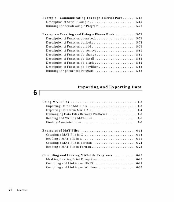
Example – Communicating Through a Serial Port . . . . . . . 5-68Description of Serial Example . . . . . . . . . . . . . . . . . . . . . . . . . . 5-69Running the serialexample Program . . . . . . . . . . . . . . . . . . . . 5-72
Example – Creating and Using a Phone Book . . . . . . . . . . . 5-73Description of Function phonebook . . . . . . . . . . . . . . . . . . . . . . 5-74Description of Function pb_lookup . . . . . . . . . . . . . . . . . . . . . . 5-78Description of Function pb_add . . . . . . . . . . . . . . . . . . . . . . . . . 5-79Description of Function pb_remove . . . . . . . . . . . . . . . . . . . . . . 5-80Description of Function pb_change . . . . . . . . . . . . . . . . . . . . . . 5-80Description of Function pb_listall . . . . . . . . . . . . . . . . . . . . . . . 5-82Description of Function pb_display . . . . . . . . . . . . . . . . . . . . . . 5-82Description of Function pb_keyfilter . . . . . . . . . . . . . . . . . . . . . 5-83Running the phonebook Program . . . . . . . . . . . . . . . . . . . . . . . 5-83
6Importing and Exporting Data
Using MAT-Files . . . . . . . . . . . . . . . . . . . . . . . . . . . . . . . . . . . . . . 6-3Importing Data to MATLAB . . . . . . . . . . . . . . . . . . . . . . . . . . . . 6-3Exporting Data from MATLAB . . . . . . . . . . . . . . . . . . . . . . . . . . 6-4Exchanging Data Files Between Platforms . . . . . . . . . . . . . . . . 6-5Reading and Writing MAT-Files . . . . . . . . . . . . . . . . . . . . . . . . . 6-6Finding Associated Files . . . . . . . . . . . . . . . . . . . . . . . . . . . . . . . 6-8
Examples of MAT-Files . . . . . . . . . . . . . . . . . . . . . . . . . . . . . . . 6-11Creating a MAT-File in C . . . . . . . . . . . . . . . . . . . . . . . . . . . . . 6-11Reading a MAT-File in C . . . . . . . . . . . . . . . . . . . . . . . . . . . . . . 6-16Creating a MAT-File in Fortran . . . . . . . . . . . . . . . . . . . . . . . . 6-21Reading a MAT-File in Fortran . . . . . . . . . . . . . . . . . . . . . . . . . 6-24
Compiling and Linking MAT-File Programs . . . . . . . . . . . . 6-28Masking Floating Point Exceptions . . . . . . . . . . . . . . . . . . . . . 6-28Compiling and Linking on UNIX . . . . . . . . . . . . . . . . . . . . . . . 6-29Compiling and Linking on Windows . . . . . . . . . . . . . . . . . . . . . 6-30
vii
7ActiveX and DDE Support
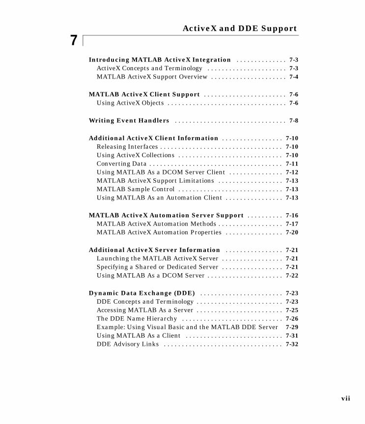
Introducing MATLAB ActiveX Integration . . . . . . . . . . . . . . 7-3ActiveX Concepts and Terminology . . . . . . . . . . . . . . . . . . . . . . 7-3MATLAB ActiveX Support Overview . . . . . . . . . . . . . . . . . . . . . 7-4
MATLAB ActiveX Client Support . . . . . . . . . . . . . . . . . . . . . . . 7-6Using ActiveX Objects . . . . . . . . . . . . . . . . . . . . . . . . . . . . . . . . . 7-6
Writing Event Handlers . . . . . . . . . . . . . . . . . . . . . . . . . . . . . . . 7-8
Additional ActiveX Client Information . . . . . . . . . . . . . . . . . 7-10Releasing Interfaces . . . . . . . . . . . . . . . . . . . . . . . . . . . . . . . . . . 7-10Using ActiveX Collections . . . . . . . . . . . . . . . . . . . . . . . . . . . . . 7-10Converting Data . . . . . . . . . . . . . . . . . . . . . . . . . . . . . . . . . . . . . 7-11Using MATLAB As a DCOM Server Client . . . . . . . . . . . . . . . 7-12MATLAB ActiveX Support Limitations . . . . . . . . . . . . . . . . . . 7-13MATLAB Sample Control . . . . . . . . . . . . . . . . . . . . . . . . . . . . . 7-13Using MATLAB As an Automation Client . . . . . . . . . . . . . . . . 7-13
MATLAB ActiveX Automation Server Support . . . . . . . . . . 7-16MATLAB ActiveX Automation Methods . . . . . . . . . . . . . . . . . . 7-17MATLAB ActiveX Automation Properties . . . . . . . . . . . . . . . . 7-20
Additional ActiveX Server Information . . . . . . . . . . . . . . . . 7-21Launching the MATLAB ActiveX Server . . . . . . . . . . . . . . . . . 7-21Specifying a Shared or Dedicated Server . . . . . . . . . . . . . . . . . 7-21Using MATLAB As a DCOM Server . . . . . . . . . . . . . . . . . . . . . 7-22
Dynamic Data Exchange (DDE) . . . . . . . . . . . . . . . . . . . . . . . 7-23DDE Concepts and Terminology . . . . . . . . . . . . . . . . . . . . . . . . 7-23Accessing MATLAB As a Server . . . . . . . . . . . . . . . . . . . . . . . . 7-25The DDE Name Hierarchy . . . . . . . . . . . . . . . . . . . . . . . . . . . . 7-26Example: Using Visual Basic and the MATLAB DDE Server 7-29Using MATLAB As a Client . . . . . . . . . . . . . . . . . . . . . . . . . . . 7-31DDE Advisory Links . . . . . . . . . . . . . . . . . . . . . . . . . . . . . . . . . 7-32
viii Contents
8Serial Port I/O
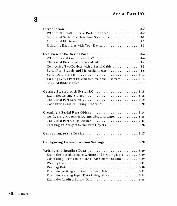
Introduction . . . . . . . . . . . . . . . . . . . . . . . . . . . . . . . . . . . . . . . . . . 8-2What Is MATLAB’s Serial Port Interface? . . . . . . . . . . . . . . . . . 8-2Supported Serial Port Interface Standards . . . . . . . . . . . . . . . . 8-2Supported Platforms . . . . . . . . . . . . . . . . . . . . . . . . . . . . . . . . . . 8-2Using the Examples with Your Device . . . . . . . . . . . . . . . . . . . . 8-3
Overview of the Serial Port . . . . . . . . . . . . . . . . . . . . . . . . . . . . 8-4What Is Serial Communication? . . . . . . . . . . . . . . . . . . . . . . . . . 8-4The Serial Port Interface Standard . . . . . . . . . . . . . . . . . . . . . . 8-4Connecting Two Devices with a Serial Cable . . . . . . . . . . . . . . . 8-5Serial Port Signals and Pin Assignments . . . . . . . . . . . . . . . . . . 8-6Serial Data Format . . . . . . . . . . . . . . . . . . . . . . . . . . . . . . . . . . 8-11Finding Serial Port Information for Your Platform . . . . . . . . . 8-15Selected Bibliography . . . . . . . . . . . . . . . . . . . . . . . . . . . . . . . . 8-17
Getting Started with Serial I/O . . . . . . . . . . . . . . . . . . . . . . . . 8-18Example: Getting Started . . . . . . . . . . . . . . . . . . . . . . . . . . . . . 8-18The Serial Port Session . . . . . . . . . . . . . . . . . . . . . . . . . . . . . . . 8-19Configuring and Returning Properties . . . . . . . . . . . . . . . . . . . 8-20
Creating a Serial Port Object . . . . . . . . . . . . . . . . . . . . . . . . . 8-24Configuring Properties During Object Creation . . . . . . . . . . . 8-25The Serial Port Object Display . . . . . . . . . . . . . . . . . . . . . . . . . 8-25Creating an Array of Serial Port Objects . . . . . . . . . . . . . . . . . 8-26
Connecting to the Device . . . . . . . . . . . . . . . . . . . . . . . . . . . . . 8-27
Configuring Communication Settings . . . . . . . . . . . . . . . . . . 8-28
Writing and Reading Data . . . . . . . . . . . . . . . . . . . . . . . . . . . . 8-29Example: Introduction to Writing and Reading Data . . . . . . . 8-29Controlling Access to the MATLAB Command Line . . . . . . . . 8-29Writing Data . . . . . . . . . . . . . . . . . . . . . . . . . . . . . . . . . . . . . . . 8-31Reading Data . . . . . . . . . . . . . . . . . . . . . . . . . . . . . . . . . . . . . . . 8-36Example: Writing and Reading Text Data . . . . . . . . . . . . . . . . 8-42Example: Parsing Input Data Using strread . . . . . . . . . . . . . . 8-44Example: Reading Binary Data . . . . . . . . . . . . . . . . . . . . . . . . . 8-45
ix
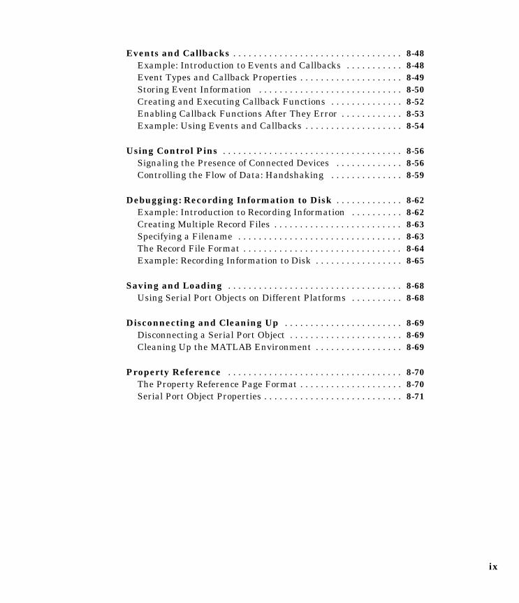
Events and Callbacks . . . . . . . . . . . . . . . . . . . . . . . . . . . . . . . . . 8-48Example: Introduction to Events and Callbacks . . . . . . . . . . . 8-48Event Types and Callback Properties . . . . . . . . . . . . . . . . . . . . 8-49Storing Event Information . . . . . . . . . . . . . . . . . . . . . . . . . . . . 8-50Creating and Executing Callback Functions . . . . . . . . . . . . . . 8-52Enabling Callback Functions After They Error . . . . . . . . . . . . 8-53Example: Using Events and Callbacks . . . . . . . . . . . . . . . . . . . 8-54
Using Control Pins . . . . . . . . . . . . . . . . . . . . . . . . . . . . . . . . . . . 8-56Signaling the Presence of Connected Devices . . . . . . . . . . . . . 8-56Controlling the Flow of Data: Handshaking . . . . . . . . . . . . . . 8-59
Debugging: Recording Information to Disk . . . . . . . . . . . . . 8-62Example: Introduction to Recording Information . . . . . . . . . . 8-62Creating Multiple Record Files . . . . . . . . . . . . . . . . . . . . . . . . . 8-63Specifying a Filename . . . . . . . . . . . . . . . . . . . . . . . . . . . . . . . . 8-63The Record File Format . . . . . . . . . . . . . . . . . . . . . . . . . . . . . . . 8-64Example: Recording Information to Disk . . . . . . . . . . . . . . . . . 8-65
Saving and Loading . . . . . . . . . . . . . . . . . . . . . . . . . . . . . . . . . . 8-68Using Serial Port Objects on Different Platforms . . . . . . . . . . 8-68
Disconnecting and Cleaning Up . . . . . . . . . . . . . . . . . . . . . . . 8-69Disconnecting a Serial Port Object . . . . . . . . . . . . . . . . . . . . . . 8-69Cleaning Up the MATLAB Environment . . . . . . . . . . . . . . . . . 8-69
Property Reference . . . . . . . . . . . . . . . . . . . . . . . . . . . . . . . . . . 8-70The Property Reference Page Format . . . . . . . . . . . . . . . . . . . . 8-70Serial Port Object Properties . . . . . . . . . . . . . . . . . . . . . . . . . . . 8-71

x Contents
1Calling C and Fortran Programs from MATLAB
Introducing MEX-Files . . . . . . . . . . . . . . . 1-3Using MEX-Files . . . . . . . . . . . . . . . . . . . 1-3The Distinction Between mx and mex Prefixes . . . . . . . 1-4
MATLAB Data . . . . . . . . . . . . . . . . . . . 1-6The MATLAB Array . . . . . . . . . . . . . . . . . 1-6Data Storage . . . . . . . . . . . . . . . . . . . . 1-6Data Types in MATLAB . . . . . . . . . . . . . . . . 1-7Using Data Types . . . . . . . . . . . . . . . . . . 1-9
Building MEX-Files . . . . . . . . . . . . . . . . . 1-11Compiler Requirements . . . . . . . . . . . . . . . . 1-11Testing Your Configuration on UNIX . . . . . . . . . . 1-12Testing Your Configuration on Windows . . . . . . . . . 1-14Specifying an Options File . . . . . . . . . . . . . . . 1-17
Custom Building MEX-Files . . . . . . . . . . . . . 1-20Who Should Read This Chapter . . . . . . . . . . . . . 1-20MEX Script Switches . . . . . . . . . . . . . . . . . 1-20Default Options File on UNIX . . . . . . . . . . . . . 1-22Default Options File on Windows . . . . . . . . . . . . 1-23Custom Building on UNIX . . . . . . . . . . . . . . . 1-24Custom Building on Windows . . . . . . . . . . . . . 1-26
Troubleshooting . . . . . . . . . . . . . . . . . . 1-32Configuration Issues . . . . . . . . . . . . . . . . . 1-32Understanding MEX-File Problems . . . . . . . . . . . 1-33Compiler and Platform-Specific Issues . . . . . . . . . . 1-37Memory Management Compatibility Issues . . . . . . . . 1-37
Additional Information . . . . . . . . . . . . . . . 1-42Files and Directories - UNIX Systems . . . . . . . . . . 1-42Files and Directories - Windows Systems . . . . . . . . . 1-44Examples . . . . . . . . . . . . . . . . . . . . . . 1-46Technical Support . . . . . . . . . . . . . . . . . . 1-48
1 Calling C and Fortran Programs from MATLAB
1-2
Although MATLAB® is a complete, self-contained environment for programming and manipulating data, it is often useful to interact with data and programs external to the MATLAB environment. MATLAB provides an interface to external programs written in the C and Fortran languages.
This section discusses the following topics:
• “Introducing MEX-Files”
• “MATLAB Data”
• “Building MEX-Files”
• “Custom Building MEX-Files”
• “Troubleshooting”
• “Additional Information”
For additional information and support in building your applications, see the section, “Additional Information” on page 1-42.
Note In platform independent discussions that refer to directory paths, this book uses the UNIX convention. For example, a general reference to the mex directory is <matlab>/extern/examples/mex.
Introducing MEX-Files
1-3
Introducing MEX-FilesYou can call your own C or Fortran subroutines from MATLAB as if they were built-in functions. MATLAB callable C and Fortran programs are referred to as MEX-files. MEX-files are dynamically linked subroutines that the MATLAB interpreter can automatically load and execute.
MEX-files have several applications:
• Large pre-existing C and Fortran programs can be called from MATLAB without having to be rewritten as M-files.
• Bottleneck computations (usually for-loops) that do not run fast enough in MATLAB can be recoded in C or Fortran for efficiency.
MEX-files are not appropriate for all applications. MATLAB is a high-productivity system whose specialty is eliminating time-consuming, low-level programming in compiled languages like Fortran or C. In general, most programming should be done in MATLAB. Don’t use the MEX facility unless your application requires it.
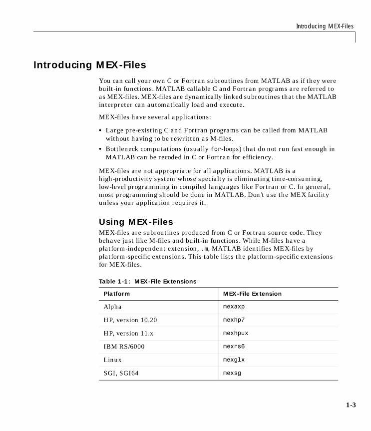
Using MEX-FilesMEX-files are subroutines produced from C or Fortran source code. They behave just like M-files and built-in functions. While M-files have a platform-independent extension, .m, MATLAB identifies MEX-files by platform-specific extensions. This table lists the platform-specific extensions for MEX-files.
Table 1-1: MEX-File Extensions
Platform MEX-File Extension
Alpha mexaxp
HP, version 10.20 mexhp7
HP, version 11.x mexhpux
IBM RS/6000 mexrs6
Linux mexglx
SGI, SGI64 mexsg
1 Calling C and Fortran Programs from MATLAB
1-4
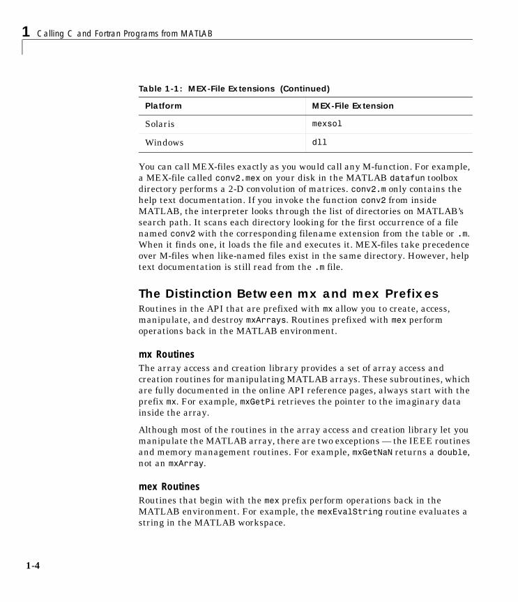
You can call MEX-files exactly as you would call any M-function. For example, a MEX-file called conv2.mex on your disk in the MATLAB datafun toolbox directory performs a 2-D convolution of matrices. conv2.m only contains the help text documentation. If you invoke the function conv2 from inside MATLAB, the interpreter looks through the list of directories on MATLAB’s search path. It scans each directory looking for the first occurrence of a file named conv2 with the corresponding filename extension from the table or .m. When it finds one, it loads the file and executes it. MEX-files take precedence over M-files when like-named files exist in the same directory. However, help text documentation is still read from the .m file.
The Distinction Between mx and mex PrefixesRoutines in the API that are prefixed with mx allow you to create, access, manipulate, and destroy mxArrays. Routines prefixed with mex perform operations back in the MATLAB environment.
mx RoutinesThe array access and creation library provides a set of array access and creation routines for manipulating MATLAB arrays. These subroutines, which are fully documented in the online API reference pages, always start with the prefix mx. For example, mxGetPi retrieves the pointer to the imaginary data inside the array.
Although most of the routines in the array access and creation library let you manipulate the MATLAB array, there are two exceptions — the IEEE routines and memory management routines. For example, mxGetNaN returns a double, not an mxArray.
mex RoutinesRoutines that begin with the mex prefix perform operations back in the MATLAB environment. For example, the mexEvalString routine evaluates a string in the MATLAB workspace.
Solaris mexsol
Windows dll
Table 1-1: MEX-File Extensions (Continued)
Platform MEX-File Extension

Introducing MEX-Files
1-5
Note mex routines are only available in MEX-functions.
1 Calling C and Fortran Programs from MATLAB
1-6
MATLAB DataBefore you can program MEX-files, you must understand how MATLAB represents the many data types it supports. This section discusses the following topics:
• “The MATLAB Array”
• “Data Storage”
• “Data Types in MATLAB”
• “Using Data Types”
The MATLAB ArrayThe MATLAB language works with only a single object type: the MATLAB array. All MATLAB variables, including scalars, vectors, matrices, strings, cell arrays, structures, and objects are stored as MATLAB arrays. In C, the MATLAB array is declared to be of type mxArray. The mxArray structure contains, among other things:
• Its type
• Its dimensions
• The data associated with this array
• If numeric, whether the variable is real or complex
• If sparse, its indices and nonzero maximum elements
• If a structure or object, the number of fields and field names
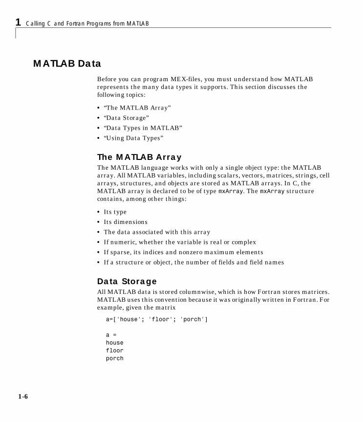
Data StorageAll MATLAB data is stored columnwise, which is how Fortran stores matrices. MATLAB uses this convention because it was originally written in Fortran. For example, given the matrix
a=['house'; 'floor'; 'porch']
a =housefloorporch
MATLAB Data
1-7
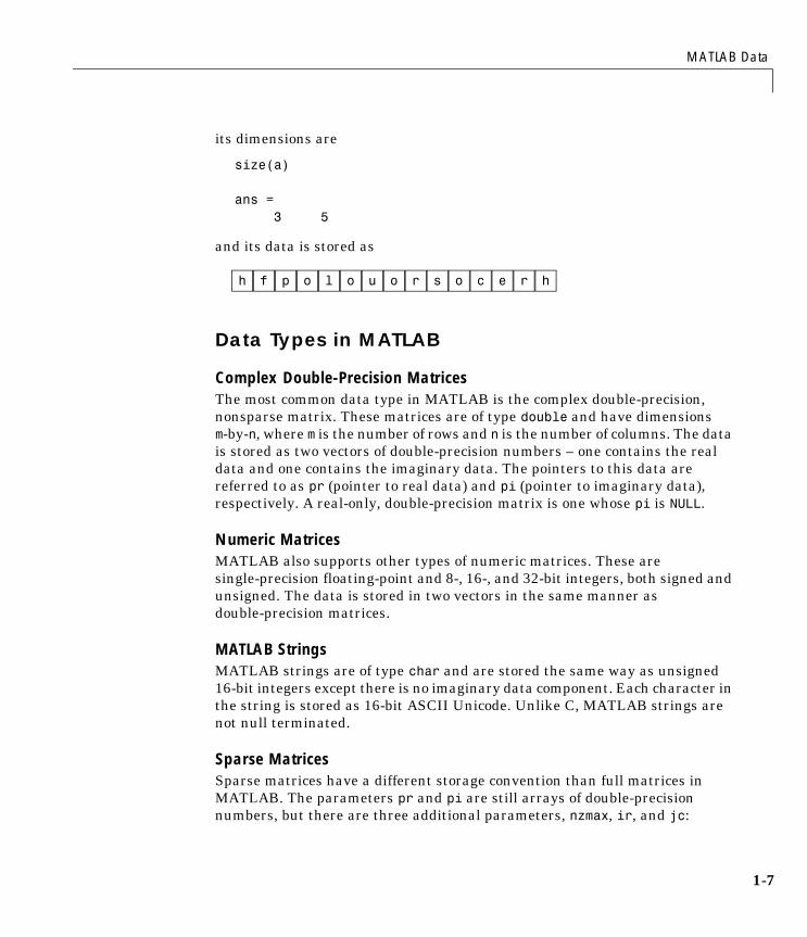
its dimensions are
size(a)
ans =3 5
and its data is stored as
Data Types in MATLAB
Complex Double-Precision MatricesThe most common data type in MATLAB is the complex double-precision, nonsparse matrix. These matrices are of type double and have dimensions m-by-n, where m is the number of rows and n is the number of columns. The data is stored as two vectors of double-precision numbers – one contains the real data and one contains the imaginary data. The pointers to this data are referred to as pr (pointer to real data) and pi (pointer to imaginary data), respectively. A real-only, double-precision matrix is one whose pi is NULL.
Numeric MatricesMATLAB also supports other types of numeric matrices. These are single-precision floating-point and 8-, 16-, and 32-bit integers, both signed and unsigned. The data is stored in two vectors in the same manner as double-precision matrices.
MATLAB StringsMATLAB strings are of type char and are stored the same way as unsigned 16-bit integers except there is no imaginary data component. Each character in the string is stored as 16-bit ASCII Unicode. Unlike C, MATLAB strings are not null terminated.
Sparse MatricesSparse matrices have a different storage convention than full matrices in MATLAB. The parameters pr and pi are still arrays of double-precision numbers, but there are three additional parameters, nzmax, ir, and jc:
h f p o l o u o r s o c e r h
1 Calling C and Fortran Programs from MATLAB
1-8
• nzmax is an integer that contains the length of ir, pr, and, if it exists, pi. It is the maximum possible number of nonzero elements in the sparse matrix.
• ir points to an integer array of length nzmax containing the row indices of the corresponding elements in pr and pi.
• jc points to an integer array of length N+1 that contains column index information. For j, in the range 0 ≤ j ≤ N-1, jc[j] is the index in ir and pr (and pi if it exists) of the first nonzero entry in the jth column and jc[j+1] - 1 index of the last nonzero entry. As a result, jc[N] is also equal to nnz, the number of nonzero entries in the matrix. If nnz is less than nzmax, then more nonzero entries can be inserted in the array without allocating additional storage.
Cell ArraysCell arrays are a collection of MATLAB arrays where each mxArray is referred to as a cell. This allows MATLAB arrays of different types to be stored together. Cell arrays are stored in a similar manner to numeric matrices, except the data portion contains a single vector of pointers to mxArrays. Members of this vector are called cells. Each cell can be of any supported data type, even another cell array.
StructuresA 1-by-1 structure is stored in the same manner as a 1-by-n cell array where n is the number of fields in the structure. Members of the data vector are called fields. Each field is associated with a name stored in the mxArray.
ObjectsObjects are stored and accessed the same way as structures. In MATLAB, objects are named structures with registered methods. Outside MATLAB, an object is a structure that contains storage for an additional classname that identifies the name of the object.
Multidimensional ArraysMATLAB arrays of any type can be multidimensional. A vector of integers is stored where each element is the size of the corresponding dimension. The storage of the data is the same as matrices.
MATLAB Data
1-9
Logical ArraysAny noncomplex numeric or sparse array can be flagged as logical. The storage for a logical array is the same as the storage for a nonlogical array.
Empty ArraysMATLAB arrays of any type can be empty. An empty mxArray is one with at least one dimension equal to zero. For example, a double-precision mxArray of type double, where m and n equal 0 and pr is NULL, is an empty array.
Using Data TypesThe six fundamental data types in MATLAB are double, char, sparse, uint8, cell, and struct. You can write MEX-files, MAT-file applications, and engine applications in C that accept any data type supported by MATLAB. In Fortran, only the creation of double-precision n-by-m arrays and strings are supported. You can treat C and Fortran MEX-files, once compiled, exactly like M-functions.
The explore ExampleThere is an example MEX-file included with MATLAB, called explore, that identifies the data type of an input variable. The source file for this example is in the <matlab>/extern/examples/mex directory, where <matlab> represents the top-level directory where MATLAB is installed on your system. For example, typing
cd([matlabroot '/extern/examples/mex']);x = 2;explore(x);
produces this result
------------------------------------------------Name: xDimensions: 1x1 Class Name: double------------------------------------------------
(1,1) = 2
1 Calling C and Fortran Programs from MATLAB
1-10
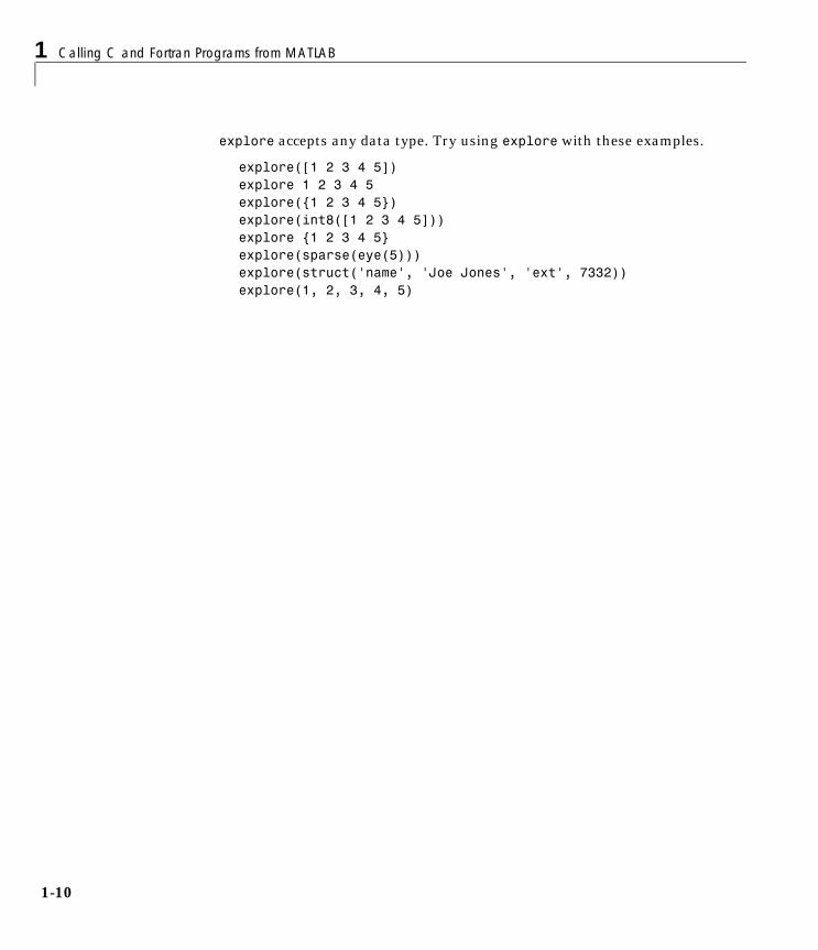
explore accepts any data type. Try using explore with these examples.
explore([1 2 3 4 5])explore 1 2 3 4 5explore({1 2 3 4 5})explore(int8([1 2 3 4 5]))explore {1 2 3 4 5}explore(sparse(eye(5)))explore(struct('name', 'Joe Jones', 'ext', 7332))explore(1, 2, 3, 4, 5)
Building MEX-Files
1-11
Building MEX-FilesThis section covers the following topics:
• “Compiler Requirements”
• “Testing Your Configuration on UNIX”
• “Testing Your Configuration on Windows”
• “Specifying an Options File”
Compiler RequirementsYour installed version of MATLAB contains all the tools you need to work with the API. MATLAB includes a C compiler for the PC called Lcc, but does not include a Fortran compiler. If you choose to use your own C compiler, it must be an ANSI C compiler. Also, if you are working on a Microsoft Windows platform, your compiler must be able to create 32-bit windows dynamically linked libraries (DLLs).
MATLAB supports many compilers and provides preconfigured files, called options files, designed specifically for these compilers. The Options Files table lists all supported compilers and their corresponding options files. The purpose of supporting this large collection of compilers is to provide you with the flexibility to use the tool of your choice. However, in many cases, you simply can use the provided Lcc compiler with your C code to produce your applications.
The MathWorks also maintains a list of compilers supported by MATLAB at the following location on the web: http://www.mathworks.com/support/tech-notes/v5/1600/1601.shtml.
Note The MathWorks provides an option (setup) for the mex script that lets you easily choose or switch your compiler.
The following sections contain configuration information for creating MEX-files on UNIX and Windows systems. More detailed information about the mex script is provided in “Custom Building MEX-Files” on page 1-20. In addition, there is a section on “Troubleshooting” on page 1-32, if you are having difficulties creating MEX-files.
1 Calling C and Fortran Programs from MATLAB
1-12
Testing Your Configuration on UNIXThe quickest way to check if your system is set up properly to create MEX-files is by trying the actual process. There is C source code for an example, yprime.c, and its Fortran counterpart, yprimef.F and yprimefg.F, included in the <matlab>/extern/examples/mex directory, where <matlab> represents the top-level directory where MATLAB is installed on your system.
To compile and link the example source files, yprime.c or yprimef.F and yprimefg.F, on UNIX, you must first copy the file(s) to a local directory, and then change directory (cd) to that local directory.
At the MATLAB prompt, type
mex yprime.c
This uses the system compiler to create the MEX-file called yprime with the appropriate extension for your system.
You can now call yprime as if it were an M-function.
yprime(1,1:4)ans = 2.0000 8.9685 4.0000 -1.0947
To try the Fortran version of the sample program with your Fortran compiler, at the MATLAB prompt, type
mex yprimef.F yprimefg.F
In addition to running the mex script from the MATLAB prompt, you can also run the script from the system prompt.
Selecting a CompilerTo change your default compiler, you select a different options file. You can do this anytime by using the command
mex -setup
Using the 'mex -setup' command selects an options file that is placed in ~/matlab and used by default for 'mex'. An options file in the current working directory or specified on the command line overrides the default options file in ~/matlab.
Building MEX-Files
1-13
Options files control which compiler to use, the compiler and link command options, and the runtime libraries to link against.
To override the default options file, use the 'mex -f' command (see 'mex -help' for more information).
The options files available for mex are:
1: <matlab>/bin/gccopts.sh : Template Options file for building gcc MEXfiles
2: <matlab>/bin/mexopts.sh : Template Options file for building MEXfiles using the system ANSI compiler
Enter the number of the options file to use as your default options file:
Select the proper options file for your system by entering its number and pressing Return. If an options file doesn’t exist in your MATLAB directory, the system displays a message stating that the options file is being copied to your user-specific matlab directory. If an options file already exists in your matlab directory, the system prompts you to overwrite it.
Note The setup option creates a user-specific matlab directory in your individual home directory and copies the appropriate options file to the directory. (If the directory already exists, a new one is not created.) This matlab directory is used for your individual options files only; each user can have his or her own default options files (other MATLAB products may place options files in this directory). Do not confuse these user-specific matlab directories with the system matlab directory, where MATLAB is installed. To see the name of this directory on your machine, use the MATLAB command prefdir.
Using the setup option resets your default compiler so that the new compiler is used every time you use the mex script.
1 Calling C and Fortran Programs from MATLAB
1-14
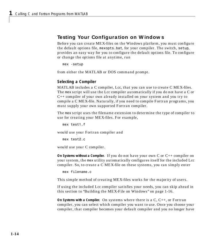
Testing Your Configuration on WindowsBefore you can create MEX-files on the Windows platform, you must configure the default options file, mexopts.bat, for your compiler. The switch, setup, provides an easy way for you to configure the default options file. To configure or change the options file at anytime, run
mex -setup
from either the MATLAB or DOS command prompt.
Selecting a CompilerMATLAB includes a C compiler, Lcc, that you can use to create C MEX-files. The mex script will use the Lcc compiler automatically if you do not have a C or C++ compiler of your own already installed on your system and you try to compile a C MEX-file. Naturally, if you need to compile Fortran programs, you must supply your own supported Fortran compiler.
The mex script uses the filename extension to determine the type of compiler to use for creating your MEX-files. For example,
mex test1.f
would use your Fortran compiler and
mex test2.c
would use your C compiler.
On Systems without a Compiler. If you do not have your own C or C++ compiler on your system, the mex utility automatically configures itself for the included Lcc compiler. So, to create a C MEX-file on these systems, you can simply enter
mex filename.c
This simple method of creating MEX-files works for the majority of users.
If using the included Lcc compiler satisfies your needs, you can skip ahead in this section to “Building the MEX-File on Windows” on page 1-16.
On Systems with a Compiler. On systems where there is a C, C++, or Fortran compiler, you can select which compiler you want to use. Once you choose your compiler, that compiler becomes your default compiler and you no longer have

Building MEX-Files
1-15
to select one when you compile MEX-files. To select a compiler or change to existing default compiler, use mex –setup.
This example shows the process of setting your default compiler to the Microsoft Visual C++ Version 6.0 compiler.
mex -setup
Please choose your compiler for building external interface (MEX) files.
Would you like mex to locate installed compilers [y]/n? n
Select a compiler:[1] Borland C++Builder version 5.0[2] Borland C++Builder version 4.0[3] Borland C++Builder version 3.0[4] Borland C/C++ version 5.02[5] Borland C/C++ version 5.0[6] Compaq Visual Fortran version 6.1[7] Digital Visual Fortran version 5.0[8] Lcc C version 2.4[9] Microsoft Visual C/C++ version 6.0[10] Microsoft Visual C/C++ version 5.0[11] WATCOM C/C++ version 11[12] WATCOM C/C++ version 10.6
[0] None
Compiler: 9
Your machine has a Microsoft Visual C/C++ compiler located at D:\Applications\Microsoft Visual Studio. Do you want to use this compiler [y]/n? y
Please verify your choices:
Compiler: Microsoft Visual C/C++ 6.0Location: D:\Applications\Microsoft Visual Studio
Are these correct?([y]/n): y
1 Calling C and Fortran Programs from MATLAB
1-16
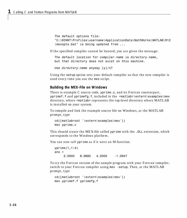
The default options file:"C:\WINNT\Profiles\username\ApplicationData\MathWorks\MATLAB\R12\mexopts.bat" is being updated from ...
If the specified compiler cannot be located, you are given the message:
The default location for compiler-name is directory-name,but that directory does not exist on this machine.
Use directory-name anyway [y]/n?
Using the setup option sets your default compiler so that the new compiler is used every time you use the mex script.
Building the MEX-File on WindowsThere is example C source code, yprime.c, and its Fortran counterpart, yprimef.f and yprimefg.f, included in the <matlab>\extern\examples\mex directory, where <matlab> represents the top-level directory where MATLAB is installed on your system.
To compile and link the example source file on Windows, at the MATLAB prompt, type
cd([matlabroot '\extern\examples\mex'])mex yprime.c
This should create the MEX-file called yprime with the .DLL extension, which corresponds to the Windows platform.
You can now call yprime as if it were an M-function.
yprime(1,1:4)ans = 2.0000 8.9685 4.0000 -1.0947
To try the Fortran version of the sample program with your Fortran compiler, switch to your Fortran compiler using mex -setup. Then, at the MATLAB prompt, type
cd([matlabroot '\extern\examples\mex'])mex yprimef.f yprimefg.f
Building MEX-Files
1-17
In addition to running the mex script from the MATLAB prompt, you can also run the script from the system prompt.
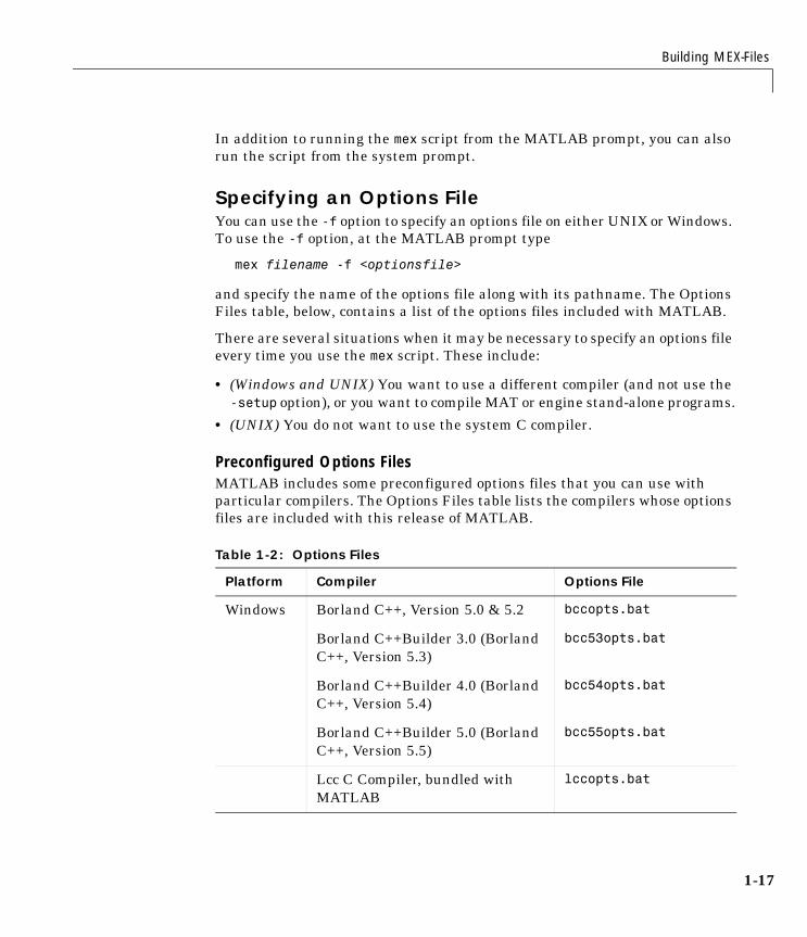
Specifying an Options FileYou can use the -f option to specify an options file on either UNIX or Windows. To use the -f option, at the MATLAB prompt type
mex filename -f <optionsfile>
and specify the name of the options file along with its pathname. The Options Files table, below, contains a list of the options files included with MATLAB.
There are several situations when it may be necessary to specify an options file every time you use the mex script. These include:
• (Windows and UNIX) You want to use a different compiler (and not use the -setup option), or you want to compile MAT or engine stand-alone programs.
• (UNIX) You do not want to use the system C compiler.
Preconfigured Options FilesMATLAB includes some preconfigured options files that you can use with particular compilers. The Options Files table lists the compilers whose options files are included with this release of MATLAB.
Table 1-2: Options Files
Platform Compiler Options File
Windows Borland C++, Version 5.0 & 5.2 bccopts.bat
Borland C++Builder 3.0 (Borland C++, Version 5.3)
bcc53opts.bat
Borland C++Builder 4.0 (Borland C++, Version 5.4)
bcc54opts.bat
Borland C++Builder 5.0 (Borland C++, Version 5.5)
bcc55opts.bat
Lcc C Compiler, bundled with MATLAB
lccopts.bat
1 Calling C and Fortran Programs from MATLAB
1-18
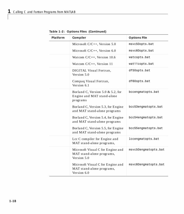
Microsoft C/C++, Version 5.0 msvc50opts.bat
Microsoft C/C++, Version 6.0 msvc60opts.bat
Watcom C/C++, Version 10.6 watcopts.bat
Watcom C/C++, Version 11 wat11copts.bat
DIGITAL Visual Fortran, Version 5.0
df50opts.bat
Compaq Visual Fortran, Version 6.1
df60opts.bat
Borland C, Version 5.0 & 5.2, for Engine and MAT stand-alone programs
bccengmatopts.bat
Borland C, Version 5.3, for Engine and MAT stand-alone programs
bcc53engmatopts.bat
Borland C, Version 5.4, for Engine and MAT stand-alone programs
bcc54engmatopts.bat
Borland C, Version 5.5, for Engine and MAT stand-alone programs
bcc55engmatopts.bat
Lcc C compiler for Engine and MAT stand-alone programs,
lccengmatopts.bat
Microsoft Visual C for Engine and MAT stand-alone programs, Version 5.0
msvc50engmatopts.bat
Microsoft Visual C for Engine and MAT stand-alone programs, Version 6.0
msvc60engmatopts.bat
Table 1-2: Options Files (Continued)
Platform Compiler Options File
Building MEX-Files
1-19
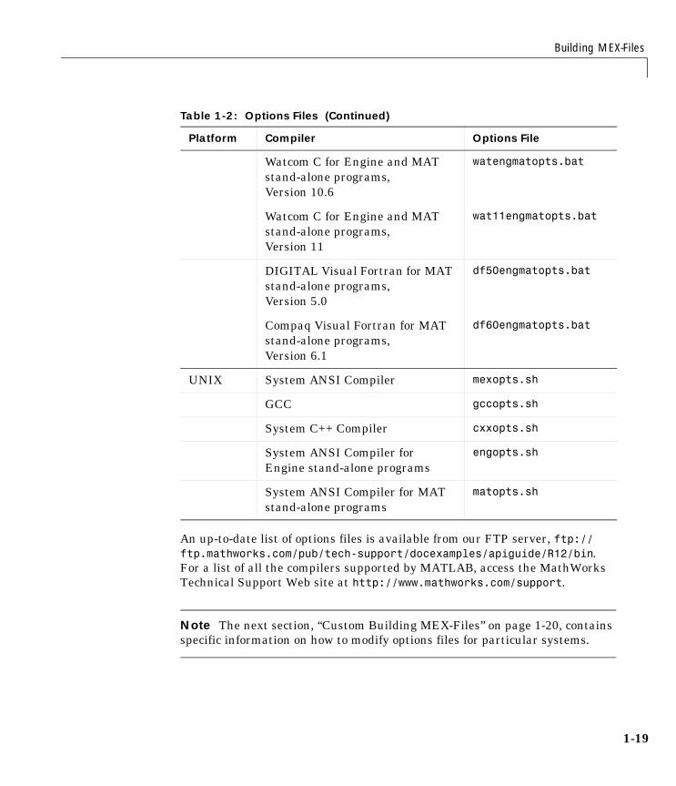
An up-to-date list of options files is available from our FTP server, ftp://ftp.mathworks.com/pub/tech-support/docexamples/apiguide/R12/bin. For a list of all the compilers supported by MATLAB, access the MathWorks Technical Support Web site at http://www.mathworks.com/support.
Note The next section, “Custom Building MEX-Files” on page 1-20, contains specific information on how to modify options files for particular systems.
Watcom C for Engine and MAT stand-alone programs, Version 10.6
watengmatopts.bat
Watcom C for Engine and MAT stand-alone programs, Version 11
wat11engmatopts.bat
DIGITAL Visual Fortran for MAT stand-alone programs, Version 5.0
df50engmatopts.bat
Compaq Visual Fortran for MAT stand-alone programs, Version 6.1
df60engmatopts.bat
UNIX System ANSI Compiler mexopts.sh
GCC gccopts.sh
System C++ Compiler cxxopts.sh
System ANSI Compiler for Engine stand-alone programs
engopts.sh
System ANSI Compiler for MAT stand-alone programs
matopts.sh
Table 1-2: Options Files (Continued)
Platform Compiler Options File
1 Calling C and Fortran Programs from MATLAB
1-20
Custom Building MEX-FilesThis section discusses in detail the process that the MEX-file build script uses. It covers the following topics:
• “Who Should Read This Chapter”
• “MEX Script Switches”
• “Default Options File on UNIX”
• “Default Options File on Windows”
• “Custom Building on UNIX”
• “Custom Building on Windows”
Who Should Read This ChapterIn general, the defaults that come with MATLAB should be sufficient for building most MEX-files. There are reasons that you might need more detailed information, such as:
• You want to use an Integrated Development Environment (IDE), rather than the provided script, to build MEX-files.
• You want to create a new options file, for example, to use a compiler that is not directly supported.
• You want to exercise more control over the build process than the script uses.
The script, in general, uses two stages (or three, for Microsoft Windows) to build MEX-files. These are the compile stage and the link stage. In between these two stages, Windows compilers must perform some additional steps to prepare for linking (the prelink stage).
MEX Script SwitchesThe mex script has a set of switches (also called options) that you can use to modify the link and compile stages. The MEX Script Switches table lists the available switches and their uses. Each switch is available on both UNIX and Windows unless otherwise noted.
For customizing the build process, you should modify the options file, which contains the compiler-specific flags corresponding to the general compile, prelink, and link steps required on your system. The options file consists of a
Custom Building MEX-Files
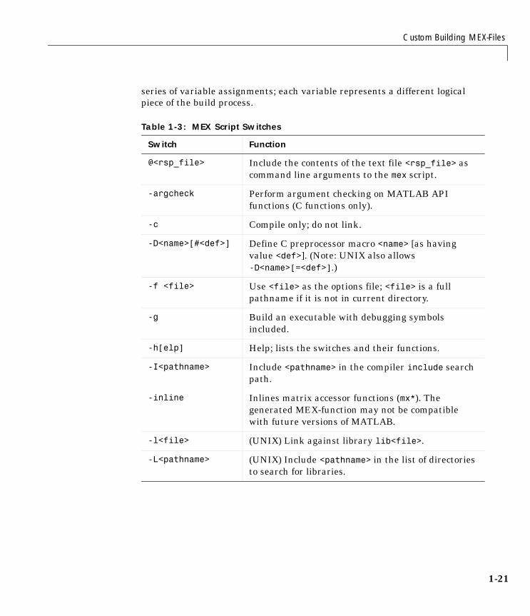
1-21
series of variable assignments; each variable represents a different logical piece of the build process.
Table 1-3: MEX Script Switches
Switch Function
@<rsp_file> Include the contents of the text file <rsp_file> as command line arguments to the mex script.
-argcheck Perform argument checking on MATLAB API functions (C functions only).
-c Compile only; do not link.
-D<name>[#<def>] Define C preprocessor macro <name> [as having value <def>]. (Note: UNIX also allows -D<name>[=<def>].)
-f <file> Use <file> as the options file; <file> is a full pathname if it is not in current directory.
-g Build an executable with debugging symbols included.
-h[elp] Help; lists the switches and their functions.
-I<pathname> Include <pathname> in the compiler include search path.
-inline Inlines matrix accessor functions (mx*). The generated MEX-function may not be compatible with future versions of MATLAB.
-l<file> (UNIX) Link against library lib<file>.
-L<pathname> (UNIX) Include <pathname> in the list of directories to search for libraries.
1 Calling C and Fortran Programs from MATLAB
1-22
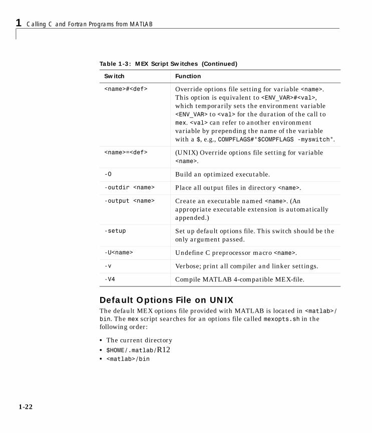
Default Options File on UNIXThe default MEX options file provided with MATLAB is located in <matlab>/bin. The mex script searches for an options file called mexopts.sh in the following order:
• The current directory• $HOME/.matlab/R12• <matlab>/bin
<name>#<def> Override options file setting for variable <name>. This option is equivalent to <ENV_VAR>#<val>, which temporarily sets the environment variable <ENV_VAR> to <val> for the duration of the call to mex. <val> can refer to another environment variable by prepending the name of the variable with a $, e.g., COMPFLAGS#"$COMPFLAGS -myswitch".
<name>=<def> (UNIX) Override options file setting for variable <name>.
-O Build an optimized executable.
-outdir <name> Place all output files in directory <name>.
-output <name> Create an executable named <name>. (An appropriate executable extension is automatically appended.)
-setup Set up default options file. This switch should be the only argument passed.
-U<name> Undefine C preprocessor macro <name>.
-v Verbose; print all compiler and linker settings.
-V4 Compile MATLAB 4-compatible MEX-file.
Table 1-3: MEX Script Switches (Continued)
Switch Function
Custom Building MEX-Files
1-23
mex uses the first occurrence of the options file it finds. If no options file is found, mex displays an error message. You can directly specify the name of the options file using the -f switch.
For specific information on the default settings for the MATLAB supported compilers, you can examine the options file in <matlab>/bin/mexopts.sh, or you can invoke the mex script in verbose mode (-v). Verbose mode will print the exact compiler options, prelink commands (if appropriate), and linker options used in the build process for each compiler. “Custom Building on UNIX” on page 1-24 gives an overview of the high-level build process.
Default Options File on WindowsThe default MEX options file is placed in your user profile directory after you configure your system by running mex -setup. The mex script searches for an options file called mexopts.bat in the following order:
• The current directory
• The user profile directory. See the following section, “The User Profile Directory”, for more information about this directory
• <matlab>\bin\win32\mexopts
mex uses the first occurrence of the options file it finds. If no options file is found, mex searches your machine for a supported C compiler and automatically configures itself to use that compiler. Also, during the configuration process, it copies the compiler’s default options file to the user profile directory. If multiple compilers are found, you are prompted to select one.
For specific information on the default settings for the MATLAB supported compilers, you can examine the options file, mexopts.bat, or you can invoke the mex script in verbose mode (-v). Verbose mode will print the exact compiler options, prelink commands, if appropriate, and linker options used in the build process for each compiler. “Custom Building on Windows” on page 1-26 gives an overview of the high-level build process.
The User Profile DirectoryThe Windows user profile directory is a directory that contains user-specific information such as desktop appearance, recently used files, and Start menu items. The mex and mbuild utilities store their respective options files, mexopts.bat and compopts.bat, which are created during the –setup process,
1 Calling C and Fortran Programs from MATLAB
1-24
in a subdirectory of your user profile directory, named Application Data\MathWorks\MATLAB. Under Windows NT and Windows 95/98 with user profiles enabled, your user profile directory is %windir%\Profiles\username. Under Windows 95/98 with user profiles disabled, your user profile directory is %windir%. Under Windows 95/98, you can determine whether or not user profiles are enabled by using the Passwords control panel.
Custom Building on UNIXOn UNIX systems, there are two stages in MEX-file building: compiling and linking.
Compile StageThe compile stage must:
• Add <matlab>/extern/include to the list of directories in which to find header files (-I<matlab>/extern/include)
• Define the preprocessor macro MATLAB_MEX_FILE (-DMATLAB_MEX_FILE)
• (C MEX-files only) Compile the source file, which contains version information for the MEX-file, <matlab>/extern/src/mexversion.c
Link StageThe link stage must:
• Instruct the linker to build a shared library
• Link all objects from compiled source files (including mexversion.c)
• (Fortran MEX-files only) Link in the precompiled versioning source file, <matlab>/extern/lib/$Arch/version4.o
• Export the symbols mexFunction and mexVersion (these symbols represent functions called by MATLAB)
For Fortran MEX-files, the symbols are all lower case and may have appended underscores. For specific information, invoke the mex script in verbose mode and examine the output.
Custom Building MEX-Files
1-25
Build OptionsFor customizing the build process, you should modify the options file. The options file contains the compiler-specific flags corresponding to the general steps outlined above. The options file consists of a series of variable assignments; each variable represents a different logical piece of the build process. The options files provided with MATLAB are located in <matlab>/bin. The section, “Default Options File on UNIX” on page 1-22, describes how the mex script looks for an options file.
To aid in providing flexibility, there are two sets of options in the options file that can be turned on and off with switches to the mex script. These sets of options correspond to building in debug mode and building in optimization mode. They are represented by the variables DEBUGFLAGS and OPTIMFLAGS, respectively, one pair for each driver that is invoked (CDEBUGFLAGS for the C compiler, FDEBUGFLAGS for the Fortran compiler, and LDDEBUGFLAGS for the linker; similarly for the OPTIMFLAGS).
• If you build in optimization mode (the default), the mex script will include the OPTIMFLAGS options in the compile and link stages.
• If you build in debug mode, the mex script will include the DEBUGFLAGS options in the compile and link stages, but will not include the OPTIMFLAGS options.
• You can include both sets of options by specifying both the optimization and debugging flags to the mex script (-O and -g, respectively).
Aside from these special variables, the mex options file defines the executable invoked for each of the three modes (C compile, Fortran compile, link) and the flags for each stage. You can also provide explicit lists of libraries that must be linked in to all MEX-files containing source files of each language.
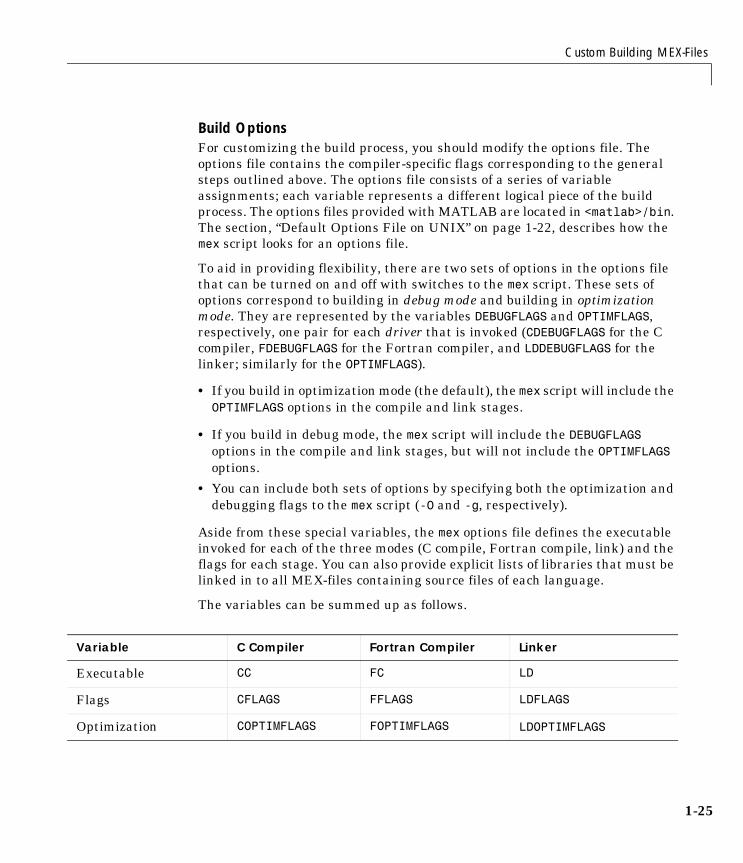
The variables can be summed up as follows.
Variable C Compiler Fortran Compiler Linker
Executable CC FC LD
Flags CFLAGS FFLAGS LDFLAGS
Optimization COPTIMFLAGS FOPTIMFLAGS LDOPTIMFLAGS
1 Calling C and Fortran Programs from MATLAB
1-26
For specifics on the default settings for these variables, you can:
• Examine the options file in <matlab>/bin/mexopts.sh (or the options file you are using), or
• Invoke the mex script in verbose mode
Custom Building on WindowsThere are three stages to MEX-file building for both C and Fortran on Windows – compiling, prelinking, and linking.
Compile StageFor the compile stage, a mex options file must:
• Set up paths to the compiler using the COMPILER (e.g., Watcom), PATH, INCLUDE, and LIB environment variables. If your compiler always has the environment variables set (e.g., in AUTOEXEC.BAT), you can remark them out in the options file.
• Define the name of the compiler, using the COMPILER environment variable, if needed.
• Define the compiler switches in the COMPFLAGS environment variable.
a The switch to create a DLL is required for MEX-files.
b For stand-alone programs, the switch to create an exe is required.
c The -c switch (compile only; do not link) is recommended.
d The switch to specify 8-byte alignment.
e Any other switch specific to the environment can be used.
• Define preprocessor macro, with -D, MATLAB_MEX_FILE is required.
• Set up optimizer switches and/or debug switches using OPTIMFLAGS and DEBUGFLAGS. These are mutually exclusive: the OPTIMFLAGS are the default,
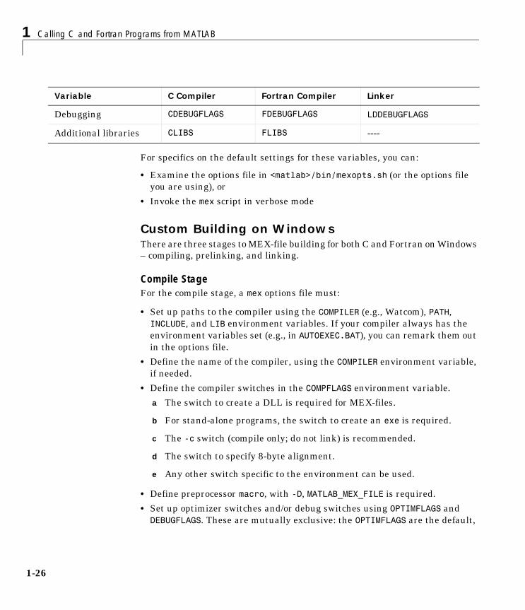
Debugging CDEBUGFLAGS FDEBUGFLAGS LDDEBUGFLAGS
Additional libraries CLIBS FLIBS ----
Variable C Compiler Fortran Compiler Linker
Custom Building MEX-Files
1-27
and the DEBUGFLAGS are used if you set the -g switch on the mex command line.
Prelink StageThe prelink stage dynamically creates import libraries to import the required function into the MEX, MAT, or engine file. All MEX-files link against MATLAB only. MAT stand-alone programs link against libmx.dll (array access library) and libmat.dll (MAT-functions). Engine stand-alone programs link against libmx.dll (array access library) and libeng.dll for engine functions. MATLAB and each DLL have corresponding .def files of the same names located in the <matlab>\extern\include directory.
Link StageFinally, for the link stage, a mex options file must:
• Define the name of the linker in the LINKER environment variable.
• Define the LINKFLAGS environment variable that must contain:
- The switch to create a DLL for MEX-files, or the switch to create an exe for stand-alone programs.
- Export of the entry point to the MEX-file as mexFunction for C or MEXFUNCTION@16 for DIGITAL Visual Fortran.
- The import library(s) created in the PRELINK_CMDS stage.
- Any other link switch specific to the compiler that can be used.
• Define the linking optimization switches and debugging switches in LINKEROPTIMFLAGS and LINKDEBUGFLAGS. As in the compile stage, these two are mutually exclusive: the default is optimization, and the -g switch invokes the debug switches.
• Define the link-file identifier in the LINK_FILE environment variable, if needed. For example, Watcom uses file to identify that the name following is a file and not a command.
• Define the link-library identifier in the LINK_LIB environment variable, if needed. For example, Watcom uses library to identify the name following is a library and not a command.
• Optionally, set up an output identifier and name with the output switch in the NAME_OUTPUT environment variable. The environment variable MEX_NAME contains the name of the first program in the command line. This must be set
1 Calling C and Fortran Programs from MATLAB
1-28
for -output to work. If this environment is not set, the compiler default is to use the name of the first program in the command line. Even if this is set, it can be overridden by specifying the mex -output switch.
Linking DLLs to MEX-FilesTo link a DLL to a MEX-file, list the DLL’s .lib file on the command line.
Versioning MEX-FilesThe mex script can build your MEX-file with a resource file that contains versioning and other essential information. The resource file is called mexversion.rc and resides in the extern\include directory. To support versioning, there are two new commands in the options files, RC_COMPILER and RC_LINKER, to provide the resource compiler and linker commands. It is assumed that:
• If a compiler command is given, the compiled resource will be linked into the MEX-file using the standard link command.
• If a linker command is given, the resource file will be linked to the MEX-file after it is built using that command.
Compiling MEX-Files with the Microsoft Visual C++ IDE
Note This section provides information on how to compile MEX-files in the Microsoft Visual C++ (MSVC) IDE; it is not totally inclusive. This section assumes that you know how to use the IDE. If you need more information on using the MSVC IDE, refer to the corresponding Microsoft documentation.
To build MEX-files with the Microsoft Visual C++ integrated development environment:
1 Create a project and insert your MEX source and mexversion.rc into it.
2 Create a .DEF file to export the MEX entry point. For example
LIBRARY MYFILE.DLLEXPORTS mexFunction <-- for a C MEX-file
orEXPORTS MEXFUNCTION@16 <-- for a Fortran MEX-file
Custom Building MEX-Files
1-29
3 Add the .DEF file to the project.
4 Locate the .LIB files for the compiler version you are using under matlabroot\extern\lib\win32\microsoft. For example, for version 6.0, these files are in the msvc60 subdirectory.
5 From this directory, add libmx.lib, libmex.lib, and libmat.lib to the library modules in the LINK settings option.
6 Add the MATLAB include directory, MATLAB\EXTERN\INCLUDE to the include path in the Settings C/C++ Preprocessor option.
7 Add MATLAB_MEX_FILE to the C/C++ Preprocessor option by selecting Settings from the Build menu, selecting C/C++, and then typing ,MATLAB_MEX_FILE after the last entry in the Preprocessor definitions field.
8 To debug the MEX-file using the IDE, put MATLAB.EXE in the Settings Debug option as the Executable for debug session.
If you are using a compiler other than the Microsoft Visual C/C++ compiler, the process for building MEX files is similar to that described above. In step 4, locate the .LIB files for the compiler you are using in a subdirectory of matlabroot\extern\lib\win32. For example, for version 5.4 of the Borland C/C++ compiler, look in matlabroot\extern\lib\win32\borland\bc54.
Using the Add-In for Visual StudioThe MathWorks provides a MATLAB add-in for the Visual Studio® development system that lets you work easily within Microsoft Visual C/C++ (MSVC). The MATLAB add-in for Visual Studio greatly simplifies using M-files in the MSVC environment. The add-in automates the integration of M-files into Visual C++ projects. It is fully integrated with the MSVC environment.
The add-in for Visual Studio is automatically installed on your system when you run either mbuild -setup or mex -setup and select Microsoft Visual C/C++ version 5 or 6. However, there are several steps you must follow in order to use the add-in:
1 To build MEX-files with the add-in for Visual Studio, run the following command at the MATLAB command prompt.
1 Calling C and Fortran Programs from MATLAB
1-30
mex -setup
Follow the menus and choose either Microsoft Visual C/C++ 5.0 or 6.0. This configures mex to use the selected Microsoft compiler and also installs the necessary add-in files in your Microsoft Visual C/C++ directories.
2 To configure the MATLAB add-in for Visual Studio to work with Microsoft Visual C/C++:
a Select Tools -> Customize from the MSVC menu.
b Click on the Add-ins and Macro Files tab.
c Check MATLAB for Visual Studio on the Add-ins and Macro Files list and click Close. The floating MATLAB add-in for Visual Studio toolbar appears. The checkmark directs MSVC to automatically load the add-in when you start MSVC again.
Configuring on Windows 95, Windows 98, and Windows ME Systems
Windows 95 and 98. To run the MATLAB add-in for Visual Studio on Windows 95 or Windows 98 systems, add this line to your config.sys file.
shell=c:\command.com /e:32768 /p
Windows ME. To run the MATLAB add-in for Visual Studio on Windows ME systems, do the following:
1 Find C:\windows\system\conagent.exe in the Windows Explorer.
2 Right click on the conagent.exe icon.
3 Select Properties from the context menu. This brings up the CONAGENT.EXE Properties window.
4 Select the Memory tab in the CONAGENT.EXE Properties window.
5 Set the Initial Environment field to 4096.
6 Click Apply.
7 Click OK.
Custom Building MEX-Files
1-31
For additional information on the MATLAB add-in for Visual Studio:
• See the MATLABAddin.hlp file in the <matlab>\bin\win32 directory, or
• Click on the Help icon in the MATLAB add-in for Visual Studio toolbar.
Help Icon
1 Calling C and Fortran Programs from MATLAB
1-32
TroubleshootingThis section explains how to troubleshoot some of the more common problems you may encounter. It addresses the following topics:
• “Configuration Issues”
• “Understanding MEX-File Problems”
• “Compiler and Platform-Specific Issues”
• “Memory Management Compatibility Issues”
Configuration IssuesThis section focuses on some common problems that might occur when creating MEX-files.
Search Path Problem on WindowsUnder Windows, if you move the MATLAB executable without reinstalling MATLAB, you may need to modify mex.bat to point to the new MATLAB location.
MATLAB Pathnames Containing Spaces on WindowsIf you have problems building MEX-files on Windows and there is a space in any of the directory names within the MATLAB path, you need to either reinstall MATLAB into a pathname that contains no spaces or rename the directory that contains the space. For example, if you install MATLAB under the Program Files directory, you may have difficulty building MEX-files with certain C compilers. Also, if you install MATLAB in a directory such as MATLAB V5.2, you may have difficulty.
DLLs Not on Path on WindowsMATLAB will fail to load MEX-files if it cannot find all DLLs referenced by the MEX-file; the DLLs must be on the DOS path or in the same directory as the MEX-file. This is also true for third-party DLLs.
Internal Error When Using mex -setup (PC).Some antivirus software packages may conflict with the mex -setup process or other mex commands. If you get an error message of the following form in response to a mex command,
Troubleshooting
1-33
mex.bat: internal error in sub get_compiler_info(): don't recognize <string>
then you need to disable your antivirus software temporarily and reenter the command. After you have successfully run the mex operation, you can re-enable your antivirus software.
Alternatively, you can open a separate MS-DOS window and enter the mex command from that window.
General Configuration ProblemMake sure you followed the configuration steps for your platform described in this chapter. Also, refer to “Custom Building MEX-Files” on page 1-20 for additional information.
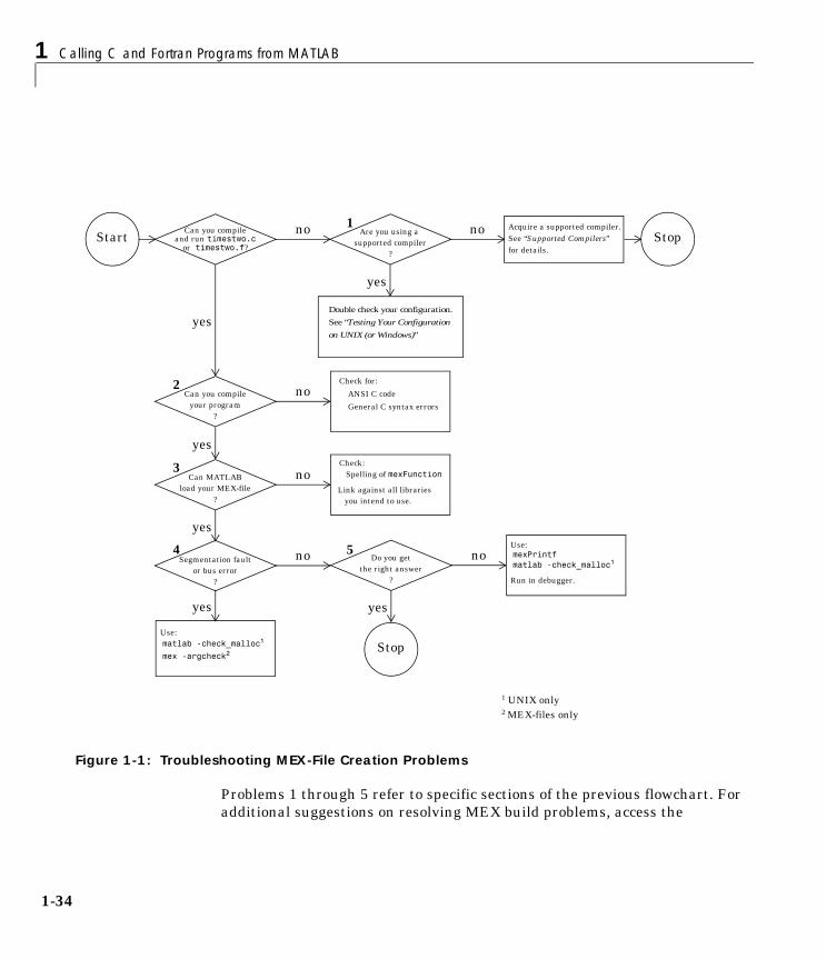
Understanding MEX-File ProblemsThis section contains information regarding common problems that occur when creating MEX-files. Use the figure, below, to help isolate these problems.
1 Calling C and Fortran Programs from MATLAB
1-34
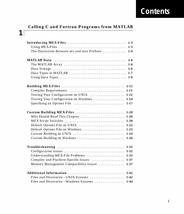
Figure 1-1: Troubleshooting MEX-File Creation Problems
Problems 1 through 5 refer to specific sections of the previous flowchart. For additional suggestions on resolving MEX build problems, access the
StartAcquire a supported compiler.See “Supported Compilers”
Can you compileand run timestwo.c
or timestwo.f?
no Are you using a supported compiler
?
no Stop
yes
Double check your configuration.
See “Testing Your Configuration
on UNIX (or Windows)”yes
Can you compileyour program
?
noCheck for:
ANSI C code
General C syntax errors
yes
Can MATLABload your MEX-file
?
no
Segmentation faultor bus error
?
Use:matlab -check_malloc1
Link against all librariesyou intend to use.
Do you getthe right answer
?
noUse:
yes
yes
matlab -check_malloc1
Run in debugger.
Stop
Check: Spelling of mexFunction
no
yes
1 UNIX only
mex -argcheck2
mexPrintf
1
2
3
4 5
2 MEX-files only
for details.
Troubleshooting
1-35
MathWorks Technical Support Web site at http://www.mathworks.com/support.
Problem 1 - Compiling a MathWorks Program FailsThe most common configuration problem in creating C MEX-files on UNIX involves using a non-ANSI C compiler, or failing to pass to the compiler a flag that tells it to compile ANSI C code.
A reliable way of knowing if you have this type of configuration problem is if the header files supplied by The MathWorks generate a string of syntax errors when you try to compile your code. See “Building MEX-Files” on page 1-11 for information on selecting the appropriate options file or, if necessary, obtain an ANSI C compiler.
Problem 2 - Compiling Your Own Program FailsA second way of generating a string of syntax errors occurs when you attempt to mix ANSI and non-ANSI C code. The MathWorks provides header and source files that are ANSI C compliant. Therefore, your C code must also be ANSI compliant.
Other common problems that can occur in any C program are neglecting to include all necessary header files, or neglecting to link against all required libraries.
Problem 3 - MEX-File Load ErrorsIf you receive an error of the form
Unable to load mex file:??? Invalid MEX-file
MATLAB is unable to recognize your MEX-file as being valid.
MATLAB loads MEX-files by looking for the gateway routine, mexFunction. If you misspell the function name, MATLAB is not able to load your MEX-file and generates an error message. On Windows, check that you are exporting mexFunction correctly.
On some platforms, if you fail to link against required libraries, you may get an error when MATLAB loads your MEX-file rather than when you compile your MEX-file. In such cases, you see a system error message referring to unresolved
1 Calling C and Fortran Programs from MATLAB
1-36
symbols or unresolved references. Be sure to link against the library that defines the function in question.
On Windows, MATLAB will fail to load MEX-files if it cannot find all DLLs referenced by the MEX-file; the DLLs must be on the path or in the same directory as the MEX-file. This is also true for third party DLLs.
Problem 4 - Segmentation Fault or Bus ErrorIf your MEX-file causes a segmentation violation or bus error, it means that the MEX-file has attempted to access protected, read-only, or unallocated memory. Since this is such a general category of programming errors, such problems are sometimes difficult to track down.
Segmentation violations do not always occur at the same point as the logical errors that cause them. If a program writes data to an unintended section of memory, an error may not occur until the program reads and interprets the corrupted data. Consequently, a segmentation violation or bus error can occur after the MEX-file finishes executing.
MATLAB provides three features to help you in troubleshooting problems of this nature. Listed in order of simplicity, they are:
• Recompile your MEX-file with argument checking (C MEX-files only). You can add a layer of error checking to your MEX-file by recompiling with the mex script flag -argcheck. This warns you about invalid arguments to both MATLAB MEX-file (mex) and matrix access (mx) API functions.
Although your MEX-file will not run as efficiently as it can, this switch detects such errors as passing null pointers to API functions.
• Run MATLAB with the -check_malloc option (UNIX only). The MATLAB startup flag, -check_malloc, indicates that MATLAB should maintain additional memory checking information. When memory is freed, MATLAB checks to make sure that memory just before and just after this memory remains unwritten and that the memory has not been previously freed.
If an error occurs, MATLAB reports the size of the allocated memory block. Using this information, you can track down where in your code this memory was allocated, and proceed accordingly.
Although using this flag prevents MATLAB from running as efficiently as it can, it detects such errors as writing past the end of a dimensioned array, or freeing previously freed memory.
Troubleshooting
1-37
• Run MATLAB within a debugging environment. This process is already described in the chapters on creating C and Fortran MEX-files, respectively.
Problem 5 - Program Generates Incorrect ResultsIf your program generates the wrong answer(s), there are several possible causes. First, there could be an error in the computational logic. Second, the program could be reading from an uninitialized section of memory. For example, reading the 11th element of a 10-element vector yields unpredictable results.
Another possibility for generating a wrong answer could be overwriting valid data due to memory mishandling. For example, writing to the 15th element of a 10-element vector might overwrite data in the adjacent variable in memory. This case can be handled in a similar manner as segmentation violations as described in Problem 4.
In all of these cases, you can use mexPrintf to examine data values at intermediate stages, or run MATLAB within a debugger to exploit all the tools the debugger provides.
Compiler and Platform-Specific IssuesThis section refers to situations specific to particular compilers and platforms.
MEX-Files Created in Watcom IDEIf you use the Watcom IDE to create MEX-files and get unresolved references to API functions when linking against our libraries, check the argument passing convention. The Watcom IDE uses a default switch that passes parameters in registers. MATLAB requires that you pass parameters on the stack.
Memory Management Compatibility IssuesTo address performance issues, we have made some changes to the internal MATLAB memory management model. These changes will allow us to provide future enhancements to the MEX-file API.
As of MATLAB 5.2, MATLAB implicitly calls mxDestroyArray, the mxArray destructor, at the end of a MEX-file’s execution on any mxArrays that are not returned in the left-hand side list (plhs[]). You are now warned if MATLAB detects any misconstructed or improperly destructed mxArrays.
1 Calling C and Fortran Programs from MATLAB
1-38
We highly recommend that you fix code in your MEX-files that produces any of the warnings discussed in the following sections. For additional information, see “Memory Management” on page 2-38 in Creating C Language MEX-Files.
Note Currently, the following warnings are enabled by default for backwards compatibility reasons. In future releases of MATLAB, the warnings will be disabled by default. The programmer will be responsible for enabling these warnings during the MEX-file development cycle.
Improperly Destroying an mxArrayYou cannot use mxFree to destroy an mxArray.
WarningWarning: You are attempting to call mxFree on a <class-id> array. The destructor for mxArrays is mxDestroyArray; please call this instead. MATLAB will attempt to fix the problem and continue, but this will result in memory faults in future releases.
Example That Causes Warning
In the following example, mxFree does not destroy the array object. This operation frees the structure header associated with the array, but MATLAB will still operate as if the array object needs to be destroyed. Thus MATLAB will try to destroy the array object, and in the process, attempt to free its structure header again.
mxArray *temp = mxCreateDoubleMatrix(1,1,mxREAL);...
mxFree(temp); /* INCORRECT */
Troubleshooting
1-39
Solution
Call mxDestroyArray instead.
mxDestroyArray(temp); /* CORRECT */
Incorrectly Constructing a Cell or Structure mxArrayYou cannot call mxSetCell or mxSetField variants with prhs[] as the member array.
Warning
Warning: You are attempting to use an array from another scope (most likely an input argument) as a member of a cell array or structure. You need to make a copy of the array first. MATLAB will attempt to fix the problem and continue, but this will result in memory faults in future releases.
Example That Causes Warning
In the following example, when the MEX-file returns, MATLAB will destroy the entire cell array. Since this includes the members of the cell, this will implicitly destroy the MEX-file’s input arguments. This can cause several strange results, generally having to do with the corruption of the caller’s workspace, if the right-hand side argument used is a temporary array (i.e., a literal or the result of an expression).
myfunction('hello')/* myfunction is the name of your MEX-file and your code *//* contains the following: */
mxArray *temp = mxCreateCellMatrix(1,1);...
mxSetCell(temp, 0, prhs[0]); /* INCORRECT */
Solution
Make a copy of the right-hand side argument with mxDuplicateArray and use that copy as the argument to mxSetCell (or mxSetField variants); for example
mxSetCell(temp, 0, mxDuplicateArray(prhs[0])); /* CORRECT */
1 Calling C and Fortran Programs from MATLAB
1-40
Creating a Temporary mxArray with Improper DataYou cannot call mxDestroyArray on an mxArray whose data was not allocated by an API routine.
Warning
Warning: You have attempted to point the data of an array to a block of memory not allocated through the MATLAB API. MATLAB will attempt to fix the problem and continue, but this will result in memory faults in future releases.
Example That Causes Warning
If you call mxSetPr, mxSetPi, mxSetData, or mxSetImagData, specifying memory that was not allocated by mxCalloc, mxMalloc, or mxRealloc as the intended data block (second argument), then when the MEX-file returns, MATLAB will attempt to free the pointer to real data and the pointer to imaginary data (if any). Thus MATLAB will attempt to free memory, in this example, from the program stack. This will cause the above warning when MATLAB attempts to reconcile its consistency checking information.
mxArray *temp = mxCreateDoubleMatrix(0,0,mxREAL); double data[5] = {1,2,3,4,5};
... mxSetM(temp,1); mxSetN(temp,5); mxSetPr(temp, data); /* INCORRECT */
Solution
Rather than use mxSetPr to set the data pointer, instead create the mxArray with the right size and use memcpy to copy the stack data into the buffer returned by mxGetPr.
mxArray *temp = mxCreateDoubleMatrix(1,5,mxREAL); double data[5] = {1,2,3,4,5};
... memcpy(mxGetPr(temp), data, 5*sizeof(double)); /* CORRECT */
Potential Memory LeaksPrior to Version 5.2, if you created an mxArray using one of the API creation routines and then you overwrote the pointer to the data using mxSetPr, MATLAB would still free the original memory. This is no longer the case.
Troubleshooting
1-41
For example,
pr = mxCalloc(5*5, sizeof(double));... <load data into pr>plhs[0] = mxCreateDoubleMatrix(5,5,mxREAL);mxSetPr(plhs[0], pr); /* INCORRECT */
will now leak 5*5*8 bytes of memory, where 8 bytes is the size of a double.
You can avoid that memory leak by changing the code
plhs[0] = mxCreateDoubleMatrix(5,5,mxREAL);pr = mxGetPr(plhs[0]);... <load data into pr>
or alternatively
pr = mxCalloc(5*5, sizeof(double));... <load data into pr>plhs[0] = mxCreateDoubleMatrix(5,5,mxREAL);mxFree(mxGetPr(plhs[0]));mxSetPr(plhs[0], pr);
Note that the first solution is more efficient.
Similar memory leaks can also occur when using mxSetPi, mxSetData, mxSetImagData, mxSetIr, or mxSetJc. You can address this issue as shown above to avoid such memory leaks.
MEX-Files Should Destroy Their Own Temporary ArraysIn general, we recommend that MEX-files destroy their own temporary arrays and clean up their own temporary memory. All mxArrays except those returned in the left-hand side list and those returned by mexGetArrayPtr may be safely destroyed. This approach is consistent with other MATLAB API applications (i.e., MAT-file applications, engine applications, and MATLAB Compiler generated applications, which do not have any automatic cleanup mechanism.)
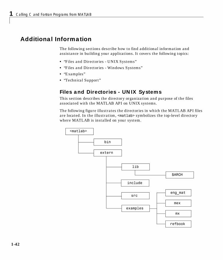
1 Calling C and Fortran Programs from MATLAB
1-42
Additional InformationThe following sections describe how to find additional information and assistance in building your applications. It covers the following topics:
• “Files and Directories - UNIX Systems”
• “Files and Directories - Windows Systems”
• “Examples”
• “Technical Support”
Files and Directories - UNIX SystemsThis section describes the directory organization and purpose of the files associated with the MATLAB API on UNIX systems.
The following figure illustrates the directories in which the MATLAB API files are located. In the illustration, <matlab> symbolizes the top-level directory where MATLAB is installed on your system.
extern
lib
bin
<matlab>
$ARCH
include
src
examplesmex
eng_mat
mx
refbook
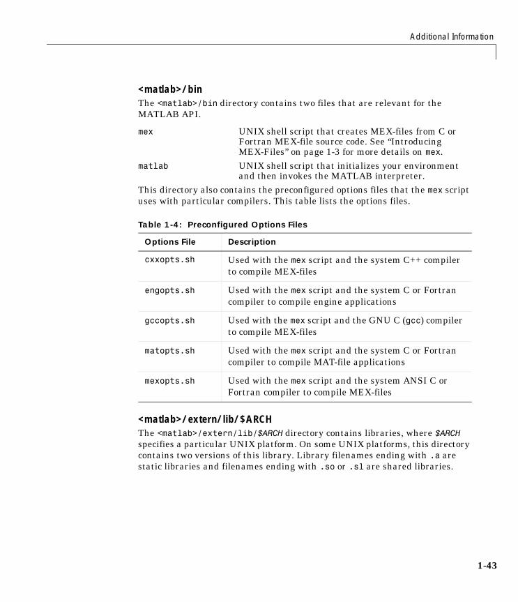
Additional Information
1-43
<matlab>/binThe <matlab>/bin directory contains two files that are relevant for the MATLAB API.
mex UNIX shell script that creates MEX-files from C or Fortran MEX-file source code. See “Introducing MEX-Files” on page 1-3 for more details on mex.
matlab UNIX shell script that initializes your environment and then invokes the MATLAB interpreter.
This directory also contains the preconfigured options files that the mex script uses with particular compilers. This table lists the options files.
<matlab>/extern/lib/$ARCHThe <matlab>/extern/lib/$ARCH directory contains libraries, where $ARCH specifies a particular UNIX platform. On some UNIX platforms, this directory contains two versions of this library. Library filenames ending with .a are static libraries and filenames ending with .so or .sl are shared libraries.
Table 1-4: Preconfigured Options Files
Options File Description
cxxopts.sh Used with the mex script and the system C++ compiler to compile MEX-files
engopts.sh Used with the mex script and the system C or Fortran compiler to compile engine applications
gccopts.sh Used with the mex script and the GNU C (gcc) compiler to compile MEX-files
matopts.sh Used with the mex script and the system C or Fortran compiler to compile MAT-file applications
mexopts.sh Used with the mex script and the system ANSI C or Fortran compiler to compile MEX-files
1 Calling C and Fortran Programs from MATLAB
1-44
<matlab>/extern/includeThe <matlab>/extern/include directory contains the header files for developing C and C++ applications that interface with MATLAB.
The relevant header files for the MATLAB API are:
engine.h Header file for MATLAB engine programs. Contains function prototypes for engine routines.
mat.h Header file for programs accessing MAT-files. Contains function prototypes for mat routines.
matrix.h Header file containing a definition of the mxArray structure and function prototypes for matrix access routines.
mex.h Header file for building MEX-files. Contains function prototypes for mex routines.
<matlab>/extern/srcThe <matlab>/extern/src directory contains those C source files that are necessary to support certain MEX-file features such as argument checking and versioning.
Files and Directories - Windows SystemsThis section describes the directory organization and purpose of the files associated with the MATLAB API on Microsoft Windows systems.
The following figure illustrates the directories in which the MATLAB API files are located. In the illustration, <matlab> symbolizes the top-level directory where MATLAB is installed on your system.
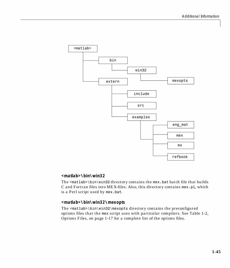
Additional Information
1-45
<matlab>\bin\win32The <matlab>\bin\win32 directory contains the mex.bat batch file that builds C and Fortran files into MEX-files. Also, this directory contains mex.pl, which is a Perl script used by mex.bat.
<matlab>\bin\win32\mexoptsThe <matlab>\bin\win32\mexopts directory contains the preconfigured options files that the mex script uses with particular compilers. See Table 1-2, Options Files, on page 1-17 for a complete list of the options files.
extern
bin
<matlab>
include
src
examples
mex
eng_mat
mx
refbook
win32
mexopts
1 Calling C and Fortran Programs from MATLAB
1-46
<matlab>\extern\includeThe <matlab>\extern\include directory contains the header files for developing C and C++ applications that interface with MATLAB.
The relevant header files for the MATLAB API (MEX-files, engine, and MAT-files) are:
engine.h Header file for MATLAB engine programs. Contains function prototypes for engine routines.
mat.h Header file for programs accessing MAT-files. Contains function prototypes for mat routines.
matrix.h Header file containing a definition of the mxArray structure and function prototypes for matrix access routines.
mex.h Header file for building MEX-files. Contains function prototypes for mex routines.
_*.def Files used by Borland compiler.*.def Files used by MSVC and Microsoft Fortran compilers.mexversion.rc Resource file for inserting versioning information into
MEX-files.
<matlab>\extern\srcThe <matlab>\extern\src directory contains files that are used for debugging MEX-files.
ExamplesThis book uses many examples to show how to write C and Fortran MEX-files.
Examples From the TextThe refbook subdirectory in the extern/examples directory contains the MEX-file examples (C and Fortran) that are used in this book, External Interfaces.
You can find the most recent versions of these examples using the anonymous FTP server locations
ftp://ftp.mathworks.com/pub/tech-support/docexamples/apiguide/R12/refbook
Additional Information
1-47
MEX Reference ExamplesThe mex subdirectory of /extern/examples directory contains MEX-file examples. It includes the examples described in the online External Interfaces/API reference pages for MEX interface functions (the functions beginning with the mex prefix).
You can find the most recent versions of these examples using the anonymous FTP server location
ftp://ftp.mathworks.com/pub/tech-support/docexamples/apiguide/R12/mex
MX ExamplesThe mx subdirectory of extern/examples contains examples for using the array access functions. Although you can use these functions in stand-alone programs, most of these are MEX-file examples. The exception is mxSetAllocFcns.c, since this function is available only to stand-alone programs.
You can find the most recent versions of these examples using the anonymous FTP server location
ftp://ftp.mathworks.com/pub/tech-support/docexamples/apiguide/R12/mx
Engine and MAT ExamplesThe eng_mat subdirectory in the extern/examples directory contains the MEX-file examples (C and Fortran) for using the MATLAB engine facility, as well as examples for reading and writing MATLAB data files (MAT-files). These examples are all stand-alone programs.
You can find the most recent versions of these examples using the anonymous FTP server locations
ftp://ftp.mathworks.com/pub/tech-support/docexamples/apiguide/R12/eng_mat
1 Calling C and Fortran Programs from MATLAB
1-48
Technical SupportThe MathWorks provides additional Technical Support through its web site. A few of the services provided are as follows:
• FAQ (Frequently Asked Questions)
This is a list of the most frequently asked questions received by our Technical Support staff, along with answers from the solutions database.
http://www.mathworks.com/support/index.shtml
• Solution Search Engine
This knowledge base on our web site includes thousands of solutions and links to Technical Notes and is updated several times each week.
http://www.mathworks.com/support/solutions/index.shtml
• Technical Notes
Technical notes are written by our Technical Support staff to address commonly asked questions.
http://www.mathworks.com/support/tech-notes/index.shtml
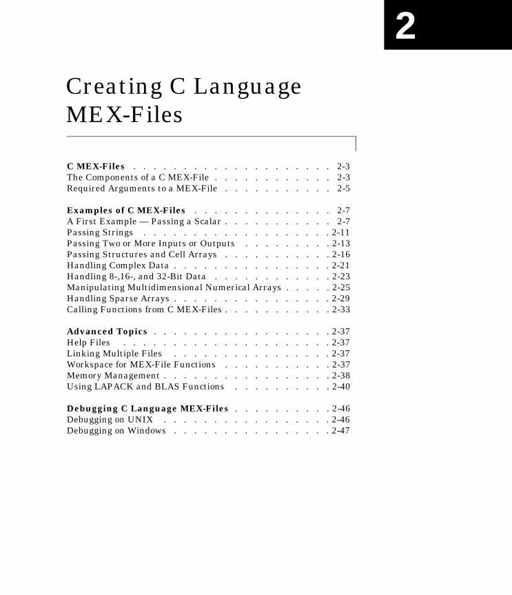
2Creating C Language MEX-Files
C MEX-Files . . . . . . . . . . . . . . . . . . . . 2-3The Components of a C MEX-File . . . . . . . . . . . . 2-3Required Arguments to a MEX-File . . . . . . . . . . . 2-5
Examples of C MEX-Files . . . . . . . . . . . . . . 2-7A First Example — Passing a Scalar . . . . . . . . . . . 2-7Passing Strings . . . . . . . . . . . . . . . . . . . 2-11Passing Two or More Inputs or Outputs . . . . . . . . . 2-13Passing Structures and Cell Arrays . . . . . . . . . . . 2-16Handling Complex Data . . . . . . . . . . . . . . . . 2-21Handling 8-,16-, and 32-Bit Data . . . . . . . . . . . . 2-23Manipulating Multidimensional Numerical Arrays . . . . . 2-25Handling Sparse Arrays . . . . . . . . . . . . . . . . 2-29Calling Functions from C MEX-Files . . . . . . . . . . . 2-33
Advanced Topics . . . . . . . . . . . . . . . . . . 2-37Help Files . . . . . . . . . . . . . . . . . . . . . 2-37Linking Multiple Files . . . . . . . . . . . . . . . . 2-37Workspace for MEX-File Functions . . . . . . . . . . . 2-37Memory Management . . . . . . . . . . . . . . . . . 2-38Using LAPACK and BLAS Functions . . . . . . . . . . 2-40
Debugging C Language MEX-Files . . . . . . . . . . 2-46Debugging on UNIX . . . . . . . . . . . . . . . . . 2-46Debugging on Windows . . . . . . . . . . . . . . . . 2-47
2 Creating C Language MEX-Files
2-2
This chapter describes how to write MEX-files in the C programming language. It discusses the MEX-file itself, how these C language files interact with MATLAB, how to pass and manipulate arguments of different data types, how to debug your MEX-file programs, and several other, more advanced topics.
The following list summarizes the contents of this chapter:
• “C MEX-Files”
• “Examples of C MEX-Files”
• “Advanced Topics”
• “Debugging C Language MEX-Files”
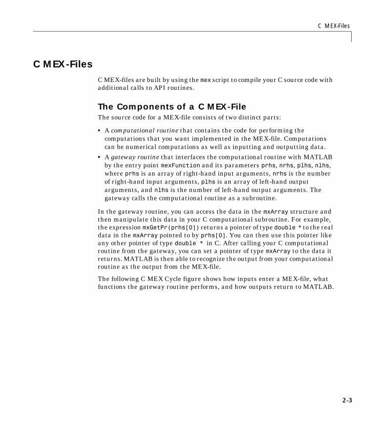
C MEX-Files
2-3
C MEX-FilesC MEX-files are built by using the mex script to compile your C source code with additional calls to API routines.
The Components of a C MEX-FileThe source code for a MEX-file consists of two distinct parts:
• A computational routine that contains the code for performing the computations that you want implemented in the MEX-file. Computations can be numerical computations as well as inputting and outputting data.
• A gateway routine that interfaces the computational routine with MATLAB by the entry point mexFunction and its parameters prhs, nrhs, plhs, nlhs, where prhs is an array of right-hand input arguments, nrhs is the number of right-hand input arguments, plhs is an array of left-hand output arguments, and nlhs is the number of left-hand output arguments. The gateway calls the computational routine as a subroutine.
In the gateway routine, you can access the data in the mxArray structure and then manipulate this data in your C computational subroutine. For example, the expression mxGetPr(prhs[0]) returns a pointer of type double * to the real data in the mxArray pointed to by prhs[0]. You can then use this pointer like any other pointer of type double * in C. After calling your C computational routine from the gateway, you can set a pointer of type mxArray to the data it returns. MATLAB is then able to recognize the output from your computational routine as the output from the MEX-file.
The following C MEX Cycle figure shows how inputs enter a MEX-file, what functions the gateway routine performs, and how outputs return to MATLAB.
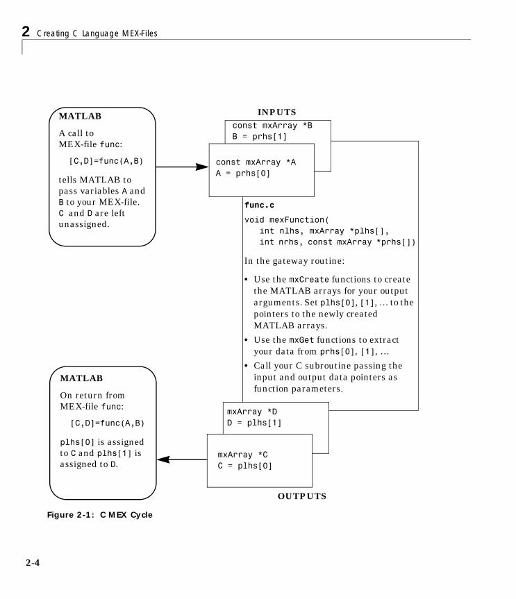
2 Creating C Language MEX-Files
2-4
Figure 2-1: C MEX Cycle
const mxArray *AA = prhs[0]
MATLAB
A call toMEX-file func:
[C,D]=func(A,B)
tells MATLAB to pass variables A and B to your MEX-file. C and D are left unassigned.
mxArray *CC = plhs[0]
const mxArray *BB = prhs[1]
mxArray *DD = plhs[1]
INPUTS
OUTPUTS
func.c
void mexFunction(int nlhs, mxArray *plhs[],int nrhs, const mxArray *prhs[])
In the gateway routine:
• Use the mxCreate functions to create the MATLAB arrays for your output arguments. Set plhs[0], [1], … to the pointers to the newly created MATLAB arrays.
• Use the mxGet functions to extract your data from prhs[0], [1], …
• Call your C subroutine passing the input and output data pointers as function parameters.
MATLAB
On return fromMEX-file func:
[C,D]=func(A,B)
plhs[0] is assigned to C and plhs[1] is assigned to D.

C MEX-Files
2-5
Required Arguments to a MEX-FileThe two components of the MEX-file may be separate or combined. In either case, the files must contain the #include "mex.h" header so that the entry point and interface routines are declared properly. The name of the gateway routine must always be mexFunction and must contain these parameters.
void mexFunction(int nlhs, mxArray *plhs[],int nrhs, const mxArray *prhs[])
{/* more C code ... */
The parameters nlhs and nrhs contain the number of left- and right-hand arguments with which the MEX-file is invoked. In the syntax of the MATLAB language, functions have the general form
[a,b,c,…] = fun(d,e,f,…)
where the ellipsis (…) denotes additional terms of the same format. The a,b,c,… are left-hand arguments and the d,e,f,… are right-hand arguments.
The parameters plhs and prhs are vectors that contain pointers to the left- and right-hand arguments of the MEX-file. Note that both are declared as containing type mxArray *, which means that the variables pointed at are MATLAB arrays. prhs is a length nrhs array of pointers to the right-hand side inputs to the MEX-file, and plhs is a length nlhs array that will contain pointers to the left-hand side outputs that your function generates.
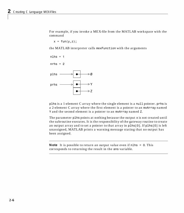
2 Creating C Language MEX-Files
2-6
For example, if you invoke a MEX-file from the MATLAB workspace with the command
x = fun(y,z);
the MATLAB interpreter calls mexFunction with the arguments
plhs is a 1-element C array where the single element is a null pointer. prhs is a 2-element C array where the first element is a pointer to an mxArray named Y and the second element is a pointer to an mxArray named Z.
The parameter plhs points at nothing because the output x is not created until the subroutine executes. It is the responsibility of the gateway routine to create an output array and to set a pointer to that array in plhs[0]. If plhs[0] is left unassigned, MATLAB prints a warning message stating that no output has been assigned.
Note It is possible to return an output value even if nlhs = 0. This corresponds to returning the result in the ans variable.
nlhs = 1
nrhs = 2
plhs
prhs
• Ø
• Y
• Z
Examples of C MEX-Files
2-7
Examples of C MEX-FilesThe following sections include information and examples describing how to pass and manipulate the different data types when working with MEX-files. These topics include
• “A First Example — Passing a Scalar”
• “Passing Strings”
• “Passing Two or More Inputs or Outputs”
• “Passing Structures and Cell Arrays”
• “Handling Complex Data”
• “Handling 8-,16-, and 32-Bit Data”
• “Manipulating Multidimensional Numerical Arrays”
• “Handling Sparse Arrays”
• “Calling Functions from C MEX-Files”
The MATLAB API provides a full set of routines that handle the various data types supported by MATLAB. For each data type there is a specific set of functions that you can use for data manipulation. The first example discusses the simple case of doubling a scalar. After that, the examples discuss how to pass in, manipulate, and pass back various data types, and how to handle multiple inputs and outputs. Finally, the sections discuss passing and manipulating various MATLAB data types.
Note You can find the most recent versions of the example programs at the anonymous FTP server
ftp://ftp.mathworks.com/pub/tech-support/docexamples/apiguide/R12/refbook
A First Example — Passing a ScalarLet’s look at a simple example of C code and its MEX-file equivalent. Here is a C computational function that takes a scalar and doubles it.
#include <math.h>void timestwo(double y[], double x[])
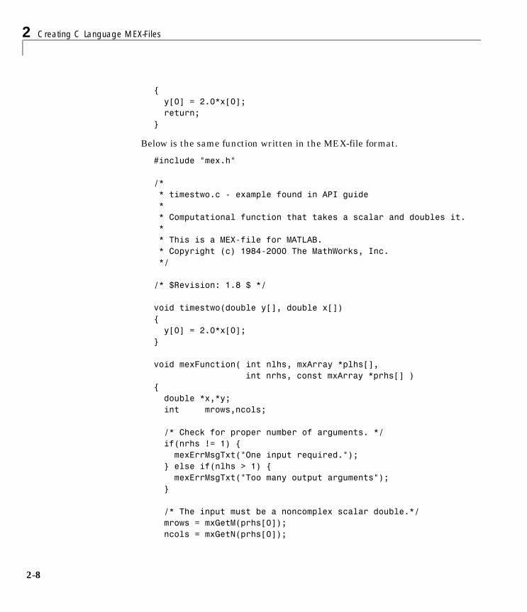
2 Creating C Language MEX-Files
2-8
{ y[0] = 2.0*x[0]; return;}
Below is the same function written in the MEX-file format.
#include "mex.h"
/* * timestwo.c - example found in API guide * * Computational function that takes a scalar and doubles it. * * This is a MEX-file for MATLAB. * Copyright (c) 1984-2000 The MathWorks, Inc. */ /* $Revision: 1.8 $ */
void timestwo(double y[], double x[]){ y[0] = 2.0*x[0];}
void mexFunction( int nlhs, mxArray *plhs[], int nrhs, const mxArray *prhs[] ){ double *x,*y; int mrows,ncols; /* Check for proper number of arguments. */ if(nrhs != 1) { mexErrMsgTxt("One input required."); } else if(nlhs > 1) { mexErrMsgTxt("Too many output arguments"); } /* The input must be a noncomplex scalar double.*/ mrows = mxGetM(prhs[0]); ncols = mxGetN(prhs[0]);
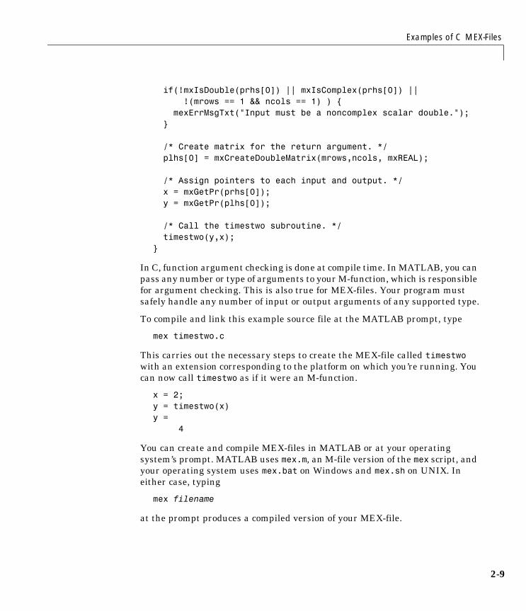
Examples of C MEX-Files
2-9
if(!mxIsDouble(prhs[0]) || mxIsComplex(prhs[0]) || !(mrows == 1 && ncols == 1) ) { mexErrMsgTxt("Input must be a noncomplex scalar double."); }
/* Create matrix for the return argument. */ plhs[0] = mxCreateDoubleMatrix(mrows,ncols, mxREAL); /* Assign pointers to each input and output. */ x = mxGetPr(prhs[0]); y = mxGetPr(plhs[0]); /* Call the timestwo subroutine. */ timestwo(y,x);}
In C, function argument checking is done at compile time. In MATLAB, you can pass any number or type of arguments to your M-function, which is responsible for argument checking. This is also true for MEX-files. Your program must safely handle any number of input or output arguments of any supported type.
To compile and link this example source file at the MATLAB prompt, type
mex timestwo.c
This carries out the necessary steps to create the MEX-file called timestwo with an extension corresponding to the platform on which you’re running. You can now call timestwo as if it were an M-function.
x = 2;y = timestwo(x)y = 4
You can create and compile MEX-files in MATLAB or at your operating system’s prompt. MATLAB uses mex.m, an M-file version of the mex script, and your operating system uses mex.bat on Windows and mex.sh on UNIX. In either case, typing
mex filename
at the prompt produces a compiled version of your MEX-file.
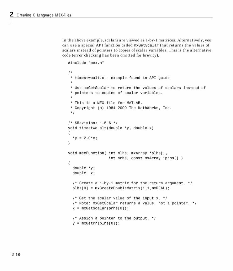
2 Creating C Language MEX-Files
2-10
In the above example, scalars are viewed as 1-by-1 matrices. Alternatively, you can use a special API function called mxGetScalar that returns the values of scalars instead of pointers to copies of scalar variables. This is the alternative code (error checking has been omitted for brevity).
#include "mex.h"
/* * timestwoalt.c - example found in API guide * * Use mxGetScalar to return the values of scalars instead of * pointers to copies of scalar variables. * * This is a MEX-file for MATLAB. * Copyright (c) 1984-2000 The MathWorks, Inc. */ /* $Revision: 1.5 $ */void timestwo_alt(double *y, double x){ *y = 2.0*x;}
void mexFunction( int nlhs, mxArray *plhs[], int nrhs, const mxArray *prhs[] ){ double *y; double x;
/* Create a 1-by-1 matrix for the return argument. */ plhs[0] = mxCreateDoubleMatrix(1,1,mxREAL);
/* Get the scalar value of the input x. */ /* Note: mxGetScalar returns a value, not a pointer. */ x = mxGetScalar(prhs[0]);
/* Assign a pointer to the output. */ y = mxGetPr(plhs[0]);
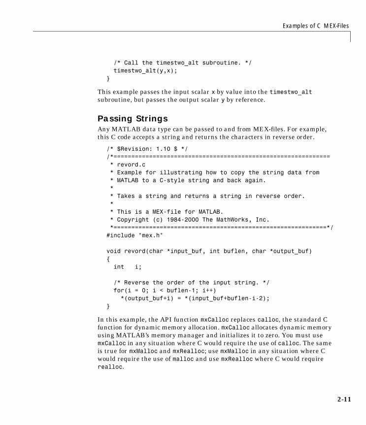
Examples of C MEX-Files
2-11
/* Call the timestwo_alt subroutine. */ timestwo_alt(y,x);}
This example passes the input scalar x by value into the timestwo_alt subroutine, but passes the output scalar y by reference.
Passing StringsAny MATLAB data type can be passed to and from MEX-files. For example, this C code accepts a string and returns the characters in reverse order.
/* $Revision: 1.10 $ *//*============================================================= * revord.c * Example for illustrating how to copy the string data from * MATLAB to a C-style string and back again. * * Takes a string and returns a string in reverse order. * * This is a MEX-file for MATLAB. * Copyright (c) 1984-2000 The MathWorks, Inc. *============================================================*/#include "mex.h"
void revord(char *input_buf, int buflen, char *output_buf){ int i;
/* Reverse the order of the input string. */ for(i = 0; i < buflen-1; i++) *(output_buf+i) = *(input_buf+buflen-i-2);}
In this example, the API function mxCalloc replaces calloc, the standard C function for dynamic memory allocation. mxCalloc allocates dynamic memory using MATLAB’s memory manager and initializes it to zero. You must use mxCalloc in any situation where C would require the use of calloc. The same is true for mxMalloc and mxRealloc; use mxMalloc in any situation where C would require the use of malloc and use mxRealloc where C would require realloc.
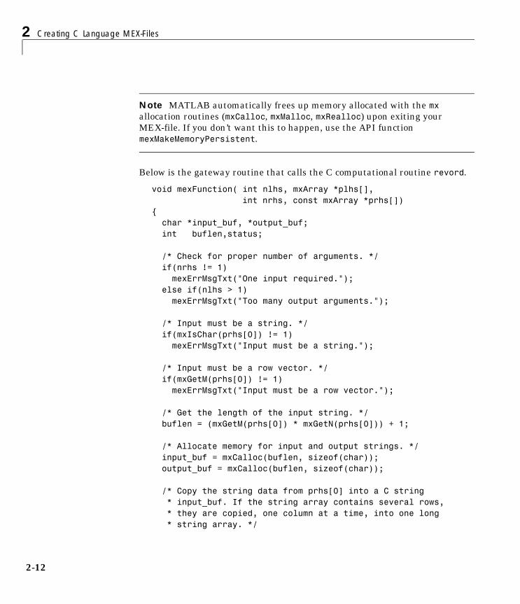
2 Creating C Language MEX-Files
2-12
Note MATLAB automatically frees up memory allocated with the mx allocation routines (mxCalloc, mxMalloc, mxRealloc) upon exiting your MEX-file. If you don’t want this to happen, use the API function mexMakeMemoryPersistent.
Below is the gateway routine that calls the C computational routine revord.
void mexFunction( int nlhs, mxArray *plhs[], int nrhs, const mxArray *prhs[]){ char *input_buf, *output_buf; int buflen,status; /* Check for proper number of arguments. */ if(nrhs != 1) mexErrMsgTxt("One input required."); else if(nlhs > 1) mexErrMsgTxt("Too many output arguments.");
/* Input must be a string. */ if(mxIsChar(prhs[0]) != 1) mexErrMsgTxt("Input must be a string.");
/* Input must be a row vector. */ if(mxGetM(prhs[0]) != 1) mexErrMsgTxt("Input must be a row vector."); /* Get the length of the input string. */ buflen = (mxGetM(prhs[0]) * mxGetN(prhs[0])) + 1;
/* Allocate memory for input and output strings. */ input_buf = mxCalloc(buflen, sizeof(char)); output_buf = mxCalloc(buflen, sizeof(char));
/* Copy the string data from prhs[0] into a C string * input_buf. If the string array contains several rows, * they are copied, one column at a time, into one long * string array. */

Examples of C MEX-Files
2-13
status = mxGetString(prhs[0], input_buf, buflen); if(status != 0) mexWarnMsgTxt("Not enough space. String is truncated."); /* Call the C subroutine. */ revord(input_buf, buflen, output_buf);
/* Set C-style string output_buf to MATLAB mexFunction output*/ plhs[0] = mxCreateString(output_buf); return;}
The gateway routine allocates memory for the input and output strings. Since these are C strings, they need to be one greater than the number of elements in the MATLAB string. Next the MATLAB string is copied to the input string. Both the input and output strings are passed to the computational subroutine (revord), which loads the output in reverse order. Note that the output buffer is a valid null-terminated C string because mxCalloc initializes the memory to 0. The API function mxCreateString then creates a MATLAB string from the C string, output_buf. Finally, plhs[0], the left-hand side return argument to MATLAB, is set to the MATLAB array you just created.
By isolating variables of type mxArray from the computational subroutine, you can avoid having to make significant changes to your original C code.
In this example, typing
x = 'hello world';y = revord(x)
produces
The string to convert is 'hello world'.y =dlrow olleh
Passing Two or More Inputs or OutputsThe plhs[] and prhs[] parameters are vectors that contain pointers to each left-hand side (output) variable and each right-hand side (input) variable, respectively. Accordingly, plhs[0] contains a pointer to the first left-hand side argument, plhs[1] contains a pointer to the second left-hand side argument,
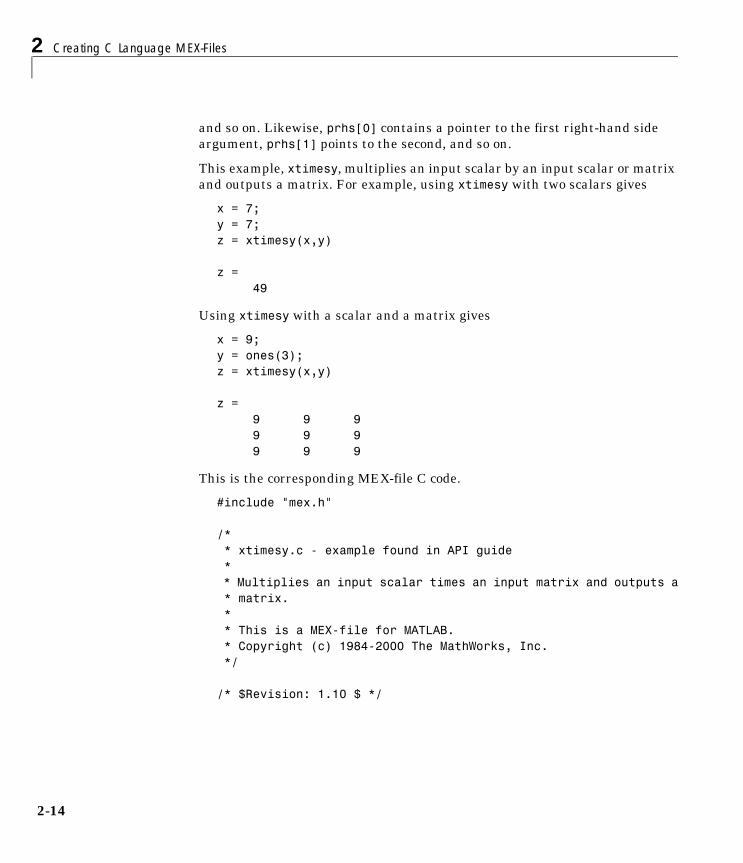
2 Creating C Language MEX-Files
2-14
and so on. Likewise, prhs[0] contains a pointer to the first right-hand side argument, prhs[1] points to the second, and so on.
This example, xtimesy, multiplies an input scalar by an input scalar or matrix and outputs a matrix. For example, using xtimesy with two scalars gives
x = 7;y = 7;z = xtimesy(x,y)
z = 49
Using xtimesy with a scalar and a matrix gives
x = 9;y = ones(3);z = xtimesy(x,y)
z = 9 9 9 9 9 9 9 9 9
This is the corresponding MEX-file C code.
#include "mex.h"
/* * xtimesy.c - example found in API guide * * Multiplies an input scalar times an input matrix and outputs a * matrix. * * This is a MEX-file for MATLAB. * Copyright (c) 1984-2000 The MathWorks, Inc. */
/* $Revision: 1.10 $ */
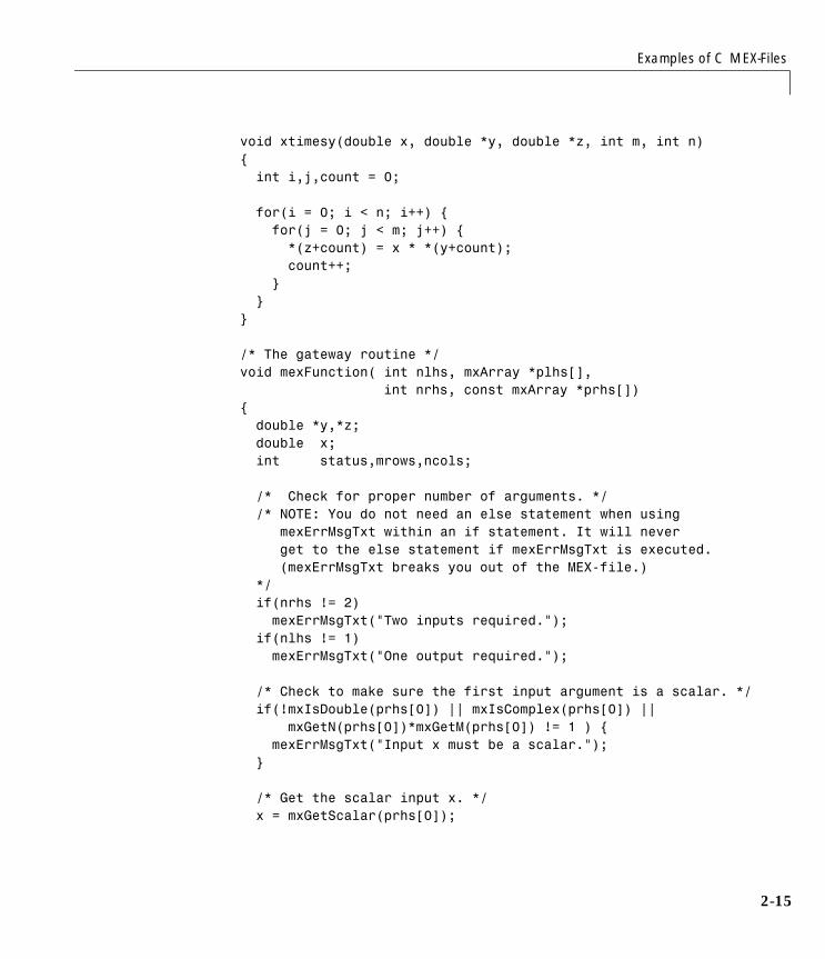
Examples of C MEX-Files
2-15
void xtimesy(double x, double *y, double *z, int m, int n){ int i,j,count = 0; for(i = 0; i < n; i++) { for(j = 0; j < m; j++) { *(z+count) = x * *(y+count); count++; } }}
/* The gateway routine */void mexFunction( int nlhs, mxArray *plhs[], int nrhs, const mxArray *prhs[]){ double *y,*z; double x; int status,mrows,ncols; /* Check for proper number of arguments. */ /* NOTE: You do not need an else statement when using mexErrMsgTxt within an if statement. It will never get to the else statement if mexErrMsgTxt is executed. (mexErrMsgTxt breaks you out of the MEX-file.) */ if(nrhs != 2) mexErrMsgTxt("Two inputs required."); if(nlhs != 1) mexErrMsgTxt("One output required."); /* Check to make sure the first input argument is a scalar. */ if(!mxIsDouble(prhs[0]) || mxIsComplex(prhs[0]) || mxGetN(prhs[0])*mxGetM(prhs[0]) != 1 ) { mexErrMsgTxt("Input x must be a scalar."); } /* Get the scalar input x. */ x = mxGetScalar(prhs[0]);
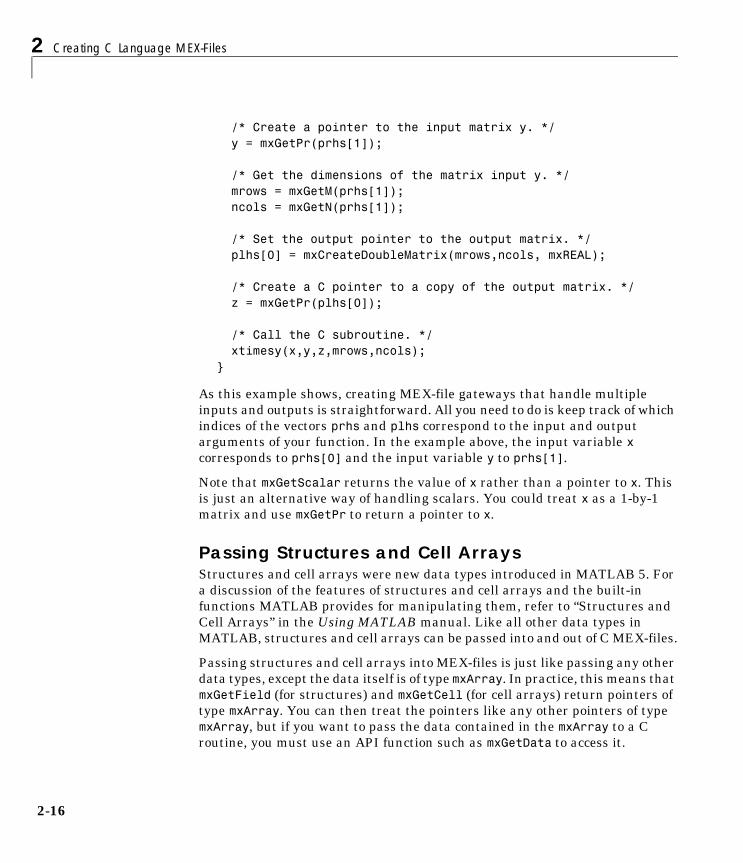
2 Creating C Language MEX-Files
2-16
/* Create a pointer to the input matrix y. */ y = mxGetPr(prhs[1]); /* Get the dimensions of the matrix input y. */ mrows = mxGetM(prhs[1]); ncols = mxGetN(prhs[1]); /* Set the output pointer to the output matrix. */ plhs[0] = mxCreateDoubleMatrix(mrows,ncols, mxREAL); /* Create a C pointer to a copy of the output matrix. */ z = mxGetPr(plhs[0]); /* Call the C subroutine. */ xtimesy(x,y,z,mrows,ncols);}
As this example shows, creating MEX-file gateways that handle multiple inputs and outputs is straightforward. All you need to do is keep track of which indices of the vectors prhs and plhs correspond to the input and output arguments of your function. In the example above, the input variable x corresponds to prhs[0] and the input variable y to prhs[1].
Note that mxGetScalar returns the value of x rather than a pointer to x. This is just an alternative way of handling scalars. You could treat x as a 1-by-1 matrix and use mxGetPr to return a pointer to x.
Passing Structures and Cell ArraysStructures and cell arrays were new data types introduced in MATLAB 5. For a discussion of the features of structures and cell arrays and the built-in functions MATLAB provides for manipulating them, refer to “Structures and Cell Arrays” in the Using MATLAB manual. Like all other data types in MATLAB, structures and cell arrays can be passed into and out of C MEX-files.
Passing structures and cell arrays into MEX-files is just like passing any other data types, except the data itself is of type mxArray. In practice, this means that mxGetField (for structures) and mxGetCell (for cell arrays) return pointers of type mxArray. You can then treat the pointers like any other pointers of type mxArray, but if you want to pass the data contained in the mxArray to a C routine, you must use an API function such as mxGetData to access it.

Examples of C MEX-Files
2-17
This example takes an m-by-n structure matrix as input and returns a new 1-by-1 structure that contains these fields:
• String input generates an m-by-n cell array
• Numeric input (noncomplex, scalar values) generates an m-by-n vector of numbers with the same class ID as the input, for example int, double, and so on.
* ============================================================= * phonebook.c * Example for illustrating how to manipulate structure and cell * array * * Takes a (MxN) structure matrix and returns a new structure * (1x1) containing corresponding fields:for string input, it * will be (MxN) cell array; and for numeric (noncomplex, scalar) * input, it will be (MxN) vector of numbers with the same * classID as input, such as int, double etc.. * * This is a MEX-file for MATLAB. * Copyright (c) 1984-2000 The MathWorks, Inc. *=============================================================*//* $Revision: 1.6 $ */
#include "mex.h"#include "string.h"
#define MAXCHARS 80 /* max length of string contained in each field */
/* the gateway routine. */void mexFunction( int nlhs, mxArray *plhs[], int nrhs, const mxArray *prhs[] ){ const char **fnames; /* pointers to field names */ const int *dims; mxArray *tmp, *fout; char *pdata; int ifield, jstruct, *classIDflags; int NStructElems, nfields, ndim;
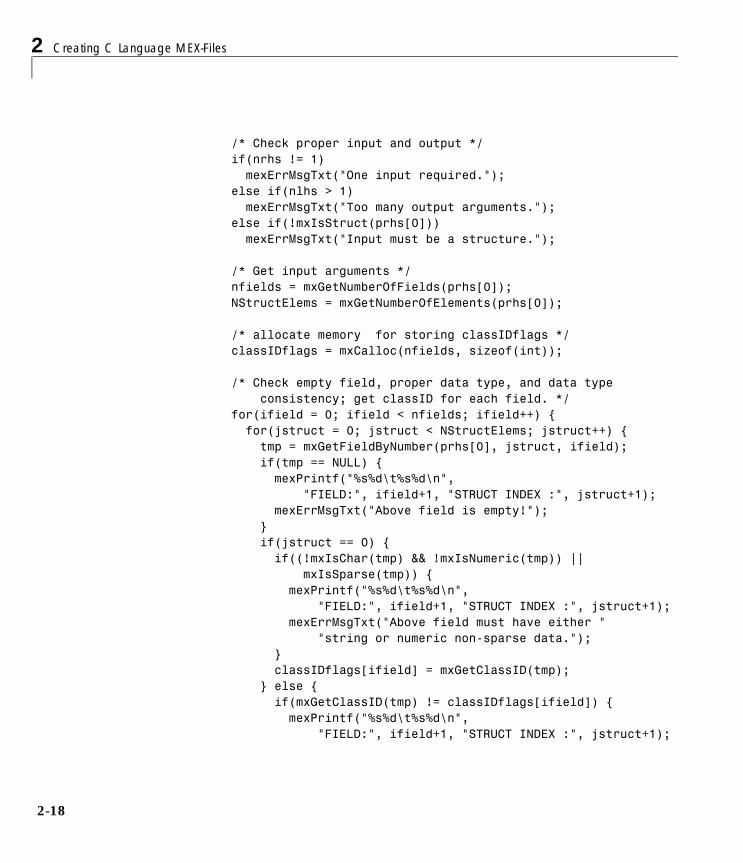
2 Creating C Language MEX-Files
2-18
/* Check proper input and output */ if(nrhs != 1) mexErrMsgTxt("One input required."); else if(nlhs > 1) mexErrMsgTxt("Too many output arguments."); else if(!mxIsStruct(prhs[0])) mexErrMsgTxt("Input must be a structure.");
/* Get input arguments */ nfields = mxGetNumberOfFields(prhs[0]); NStructElems = mxGetNumberOfElements(prhs[0]);
/* allocate memory for storing classIDflags */ classIDflags = mxCalloc(nfields, sizeof(int));
/* Check empty field, proper data type, and data type consistency; get classID for each field. */ for(ifield = 0; ifield < nfields; ifield++) { for(jstruct = 0; jstruct < NStructElems; jstruct++) { tmp = mxGetFieldByNumber(prhs[0], jstruct, ifield); if(tmp == NULL) { mexPrintf("%s%d\t%s%d\n", "FIELD:", ifield+1, "STRUCT INDEX :", jstruct+1); mexErrMsgTxt("Above field is empty!"); } if(jstruct == 0) { if((!mxIsChar(tmp) && !mxIsNumeric(tmp)) || mxIsSparse(tmp)) { mexPrintf("%s%d\t%s%d\n", "FIELD:", ifield+1, "STRUCT INDEX :", jstruct+1); mexErrMsgTxt("Above field must have either " "string or numeric non-sparse data."); } classIDflags[ifield] = mxGetClassID(tmp); } else { if(mxGetClassID(tmp) != classIDflags[ifield]) { mexPrintf("%s%d\t%s%d\n", "FIELD:", ifield+1, "STRUCT INDEX :", jstruct+1);
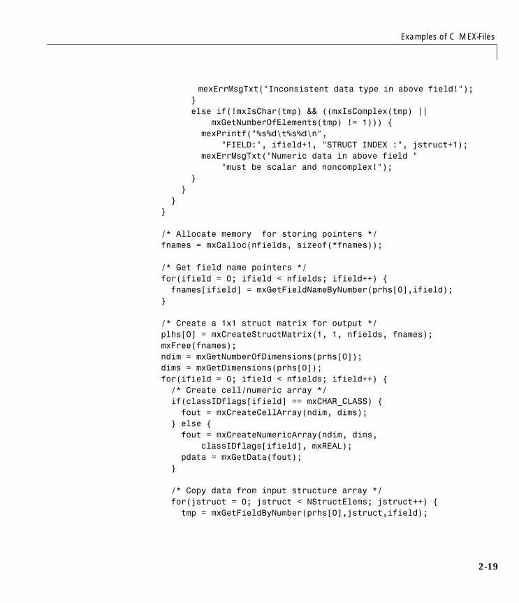
Examples of C MEX-Files
2-19
mexErrMsgTxt("Inconsistent data type in above field!"); } else if(!mxIsChar(tmp) && ((mxIsComplex(tmp) || mxGetNumberOfElements(tmp) != 1))) { mexPrintf("%s%d\t%s%d\n", "FIELD:", ifield+1, "STRUCT INDEX :", jstruct+1); mexErrMsgTxt("Numeric data in above field " "must be scalar and noncomplex!"); } } } }
/* Allocate memory for storing pointers */ fnames = mxCalloc(nfields, sizeof(*fnames));
/* Get field name pointers */ for(ifield = 0; ifield < nfields; ifield++) { fnames[ifield] = mxGetFieldNameByNumber(prhs[0],ifield); }
/* Create a 1x1 struct matrix for output */ plhs[0] = mxCreateStructMatrix(1, 1, nfields, fnames); mxFree(fnames); ndim = mxGetNumberOfDimensions(prhs[0]); dims = mxGetDimensions(prhs[0]); for(ifield = 0; ifield < nfields; ifield++) { /* Create cell/numeric array */ if(classIDflags[ifield] == mxCHAR_CLASS) { fout = mxCreateCellArray(ndim, dims); } else { fout = mxCreateNumericArray(ndim, dims, classIDflags[ifield], mxREAL); pdata = mxGetData(fout); }
/* Copy data from input structure array */ for(jstruct = 0; jstruct < NStructElems; jstruct++) { tmp = mxGetFieldByNumber(prhs[0],jstruct,ifield);
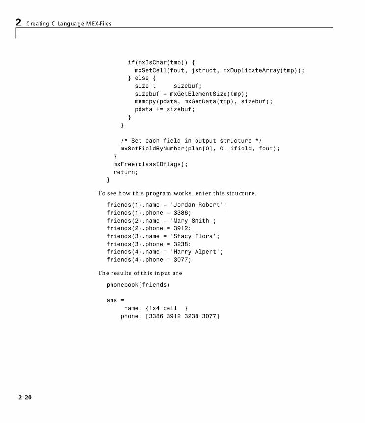
2 Creating C Language MEX-Files
2-20
if(mxIsChar(tmp)) { mxSetCell(fout, jstruct, mxDuplicateArray(tmp)); } else { size_t sizebuf; sizebuf = mxGetElementSize(tmp); memcpy(pdata, mxGetData(tmp), sizebuf); pdata += sizebuf; } }
/* Set each field in output structure */ mxSetFieldByNumber(plhs[0], 0, ifield, fout); } mxFree(classIDflags); return;}
To see how this program works, enter this structure.
friends(1).name = 'Jordan Robert';friends(1).phone = 3386;friends(2).name = 'Mary Smith';friends(2).phone = 3912;friends(3).name = 'Stacy Flora';friends(3).phone = 3238;friends(4).name = 'Harry Alpert';friends(4).phone = 3077;
The results of this input are
phonebook(friends)
ans = name: {1x4 cell } phone: [3386 3912 3238 3077]
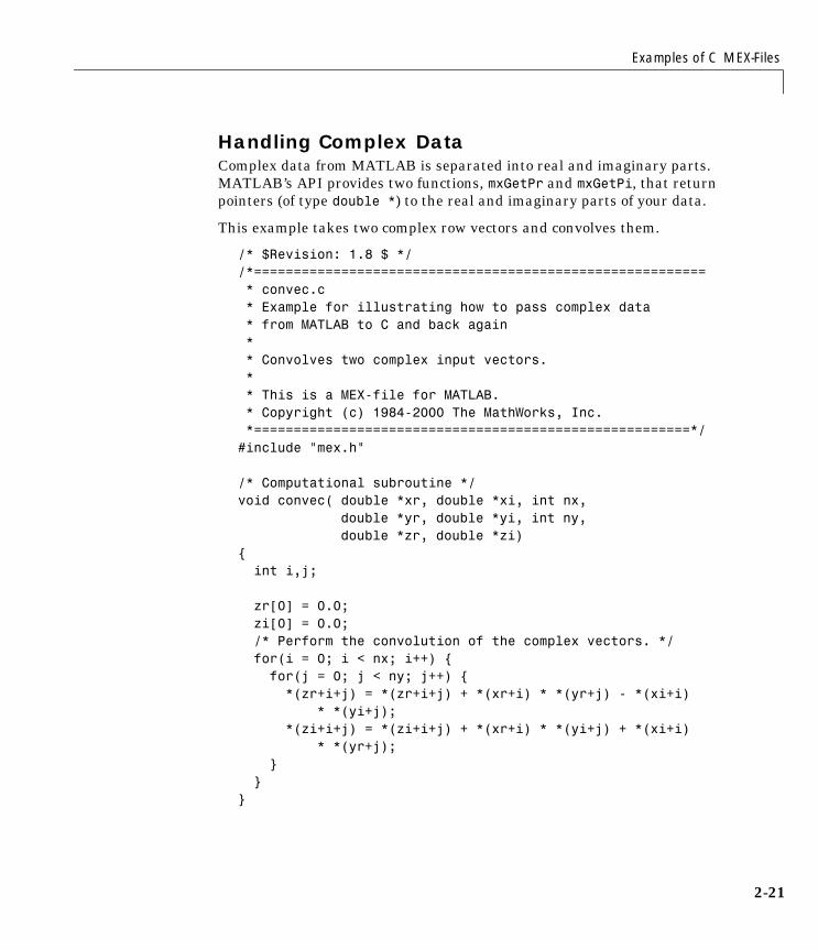
Examples of C MEX-Files
2-21
Handling Complex DataComplex data from MATLAB is separated into real and imaginary parts. MATLAB’s API provides two functions, mxGetPr and mxGetPi, that return pointers (of type double *) to the real and imaginary parts of your data.
This example takes two complex row vectors and convolves them.
/* $Revision: 1.8 $ *//*========================================================= * convec.c * Example for illustrating how to pass complex data * from MATLAB to C and back again * * Convolves two complex input vectors. * * This is a MEX-file for MATLAB. * Copyright (c) 1984-2000 The MathWorks, Inc. *=======================================================*/#include "mex.h"
/* Computational subroutine */void convec( double *xr, double *xi, int nx, double *yr, double *yi, int ny, double *zr, double *zi){ int i,j; zr[0] = 0.0; zi[0] = 0.0; /* Perform the convolution of the complex vectors. */ for(i = 0; i < nx; i++) { for(j = 0; j < ny; j++) { *(zr+i+j) = *(zr+i+j) + *(xr+i) * *(yr+j) - *(xi+i) * *(yi+j); *(zi+i+j) = *(zi+i+j) + *(xr+i) * *(yi+j) + *(xi+i) * *(yr+j); } }}
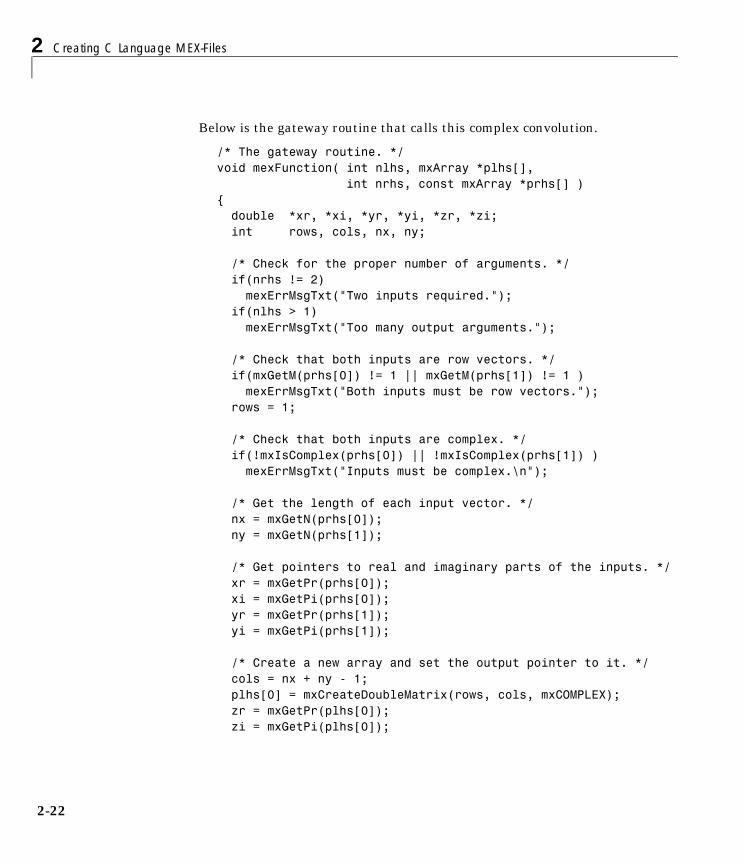
2 Creating C Language MEX-Files
2-22
Below is the gateway routine that calls this complex convolution.
/* The gateway routine. */void mexFunction( int nlhs, mxArray *plhs[], int nrhs, const mxArray *prhs[] ){ double *xr, *xi, *yr, *yi, *zr, *zi; int rows, cols, nx, ny; /* Check for the proper number of arguments. */ if(nrhs != 2) mexErrMsgTxt("Two inputs required."); if(nlhs > 1) mexErrMsgTxt("Too many output arguments.");
/* Check that both inputs are row vectors. */ if(mxGetM(prhs[0]) != 1 || mxGetM(prhs[1]) != 1 ) mexErrMsgTxt("Both inputs must be row vectors."); rows = 1;
/* Check that both inputs are complex. */ if(!mxIsComplex(prhs[0]) || !mxIsComplex(prhs[1]) ) mexErrMsgTxt("Inputs must be complex.\n"); /* Get the length of each input vector. */ nx = mxGetN(prhs[0]); ny = mxGetN(prhs[1]);
/* Get pointers to real and imaginary parts of the inputs. */ xr = mxGetPr(prhs[0]); xi = mxGetPi(prhs[0]); yr = mxGetPr(prhs[1]); yi = mxGetPi(prhs[1]); /* Create a new array and set the output pointer to it. */ cols = nx + ny - 1; plhs[0] = mxCreateDoubleMatrix(rows, cols, mxCOMPLEX); zr = mxGetPr(plhs[0]); zi = mxGetPi(plhs[0]);
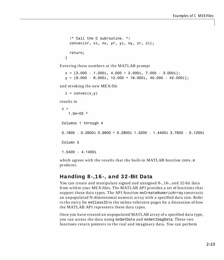
Examples of C MEX-Files
2-23
/* Call the C subroutine. */ convec(xr, xi, nx, yr, yi, ny, zr, zi);
return;}
Entering these numbers at the MATLAB prompt
x = [3.000 - 1.000i, 4.000 + 2.000i, 7.000 - 3.000i];y = [8.000 - 6.000i, 12.000 + 16.000i, 40.000 - 42.000i];
and invoking the new MEX-file
z = convec(x,y)
results in
z = 1.0e+02 *
Columns 1 through 4
0.1800 - 0.2600i 0.9600 + 0.2800i 1.3200 - 1.4400i 3.7600 - 0.1200i
Column 5
1.5400 - 4.1400i
which agrees with the results that the built-in MATLAB function conv.m produces.
Handling 8-,16-, and 32-Bit DataYou can create and manipulate signed and unsigned 8-, 16-, and 32-bit data from within your MEX-files. The MATLAB API provides a set of functions that support these data types. The API function mxCreateNumericArray constructs an unpopulated N-dimensional numeric array with a specified data size. Refer to the entry for mxClassID in the online reference pages for a discussion of how the MATLAB API represents these data types.
Once you have created an unpopulated MATLAB array of a specified data type, you can access the data using mxGetData and mxGetImagData. These two functions return pointers to the real and imaginary data. You can perform
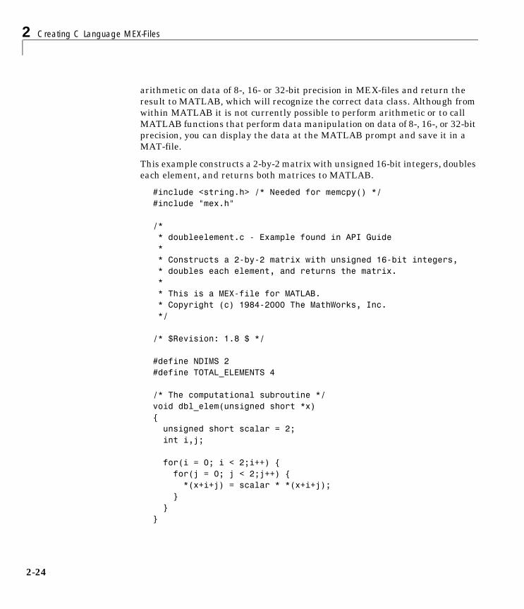
2 Creating C Language MEX-Files
2-24
arithmetic on data of 8-, 16- or 32-bit precision in MEX-files and return the result to MATLAB, which will recognize the correct data class. Although from within MATLAB it is not currently possible to perform arithmetic or to call MATLAB functions that perform data manipulation on data of 8-, 16-, or 32-bit precision, you can display the data at the MATLAB prompt and save it in a MAT-file.
This example constructs a 2-by-2 matrix with unsigned 16-bit integers, doubles each element, and returns both matrices to MATLAB.
#include <string.h> /* Needed for memcpy() */#include "mex.h"
/* * doubleelement.c - Example found in API Guide * * Constructs a 2-by-2 matrix with unsigned 16-bit integers, * doubles each element, and returns the matrix. * * This is a MEX-file for MATLAB. * Copyright (c) 1984-2000 The MathWorks, Inc. */
/* $Revision: 1.8 $ */
#define NDIMS 2#define TOTAL_ELEMENTS 4
/* The computational subroutine */void dbl_elem(unsigned short *x){ unsigned short scalar = 2; int i,j;
for(i = 0; i < 2;i++) { for(j = 0; j < 2;j++) { *(x+i+j) = scalar * *(x+i+j); } }}
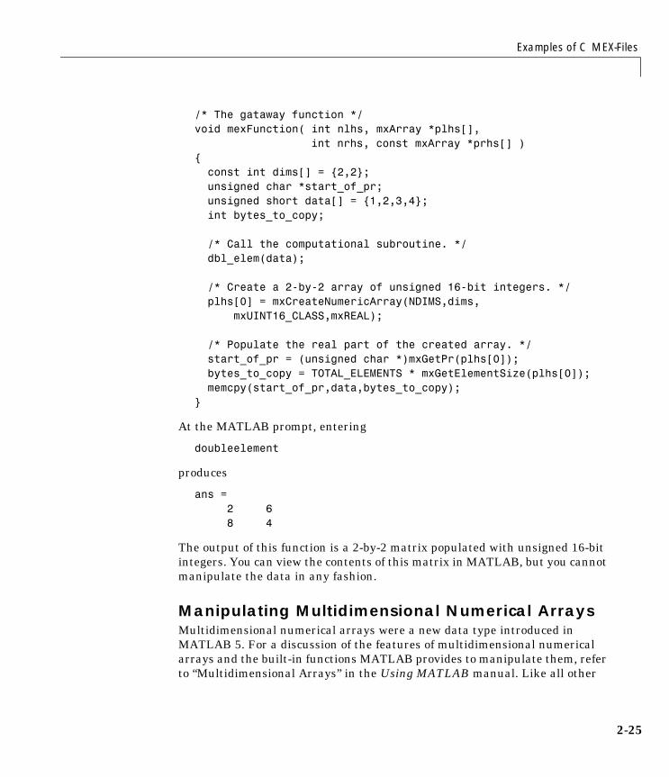
Examples of C MEX-Files
2-25
/* The gataway function */void mexFunction( int nlhs, mxArray *plhs[], int nrhs, const mxArray *prhs[] ){ const int dims[] = {2,2}; unsigned char *start_of_pr; unsigned short data[] = {1,2,3,4}; int bytes_to_copy;
/* Call the computational subroutine. */ dbl_elem(data);
/* Create a 2-by-2 array of unsigned 16-bit integers. */ plhs[0] = mxCreateNumericArray(NDIMS,dims, mxUINT16_CLASS,mxREAL);
/* Populate the real part of the created array. */ start_of_pr = (unsigned char *)mxGetPr(plhs[0]); bytes_to_copy = TOTAL_ELEMENTS * mxGetElementSize(plhs[0]); memcpy(start_of_pr,data,bytes_to_copy);}
At the MATLAB prompt, entering
doubleelement
produces
ans = 2 6 8 4
The output of this function is a 2-by-2 matrix populated with unsigned 16-bit integers. You can view the contents of this matrix in MATLAB, but you cannot manipulate the data in any fashion.
Manipulating Multidimensional Numerical ArraysMultidimensional numerical arrays were a new data type introduced in MATLAB 5. For a discussion of the features of multidimensional numerical arrays and the built-in functions MATLAB provides to manipulate them, refer to “Multidimensional Arrays” in the Using MATLAB manual. Like all other
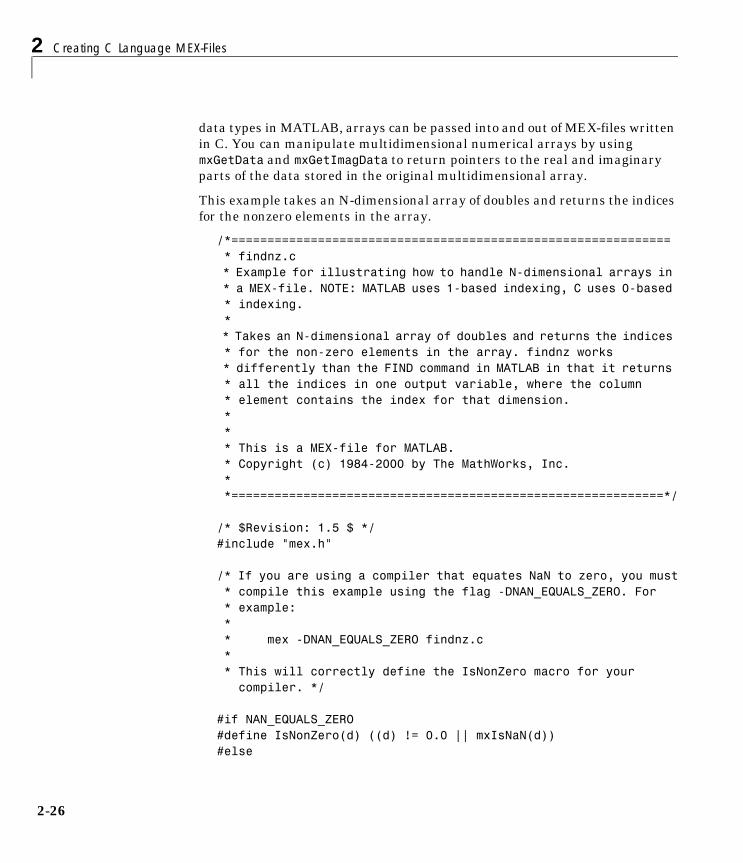
2 Creating C Language MEX-Files
2-26
data types in MATLAB, arrays can be passed into and out of MEX-files written in C. You can manipulate multidimensional numerical arrays by using mxGetData and mxGetImagData to return pointers to the real and imaginary parts of the data stored in the original multidimensional array.
This example takes an N-dimensional array of doubles and returns the indices for the nonzero elements in the array.
/*============================================================= * findnz.c * Example for illustrating how to handle N-dimensional arrays in * a MEX-file. NOTE: MATLAB uses 1-based indexing, C uses 0-based * indexing. * * Takes an N-dimensional array of doubles and returns the indices * for the non-zero elements in the array. findnz works * differently than the FIND command in MATLAB in that it returns * all the indices in one output variable, where the column * element contains the index for that dimension. * * * This is a MEX-file for MATLAB. * Copyright (c) 1984-2000 by The MathWorks, Inc. * *============================================================*/
/* $Revision: 1.5 $ */#include "mex.h"
/* If you are using a compiler that equates NaN to zero, you must * compile this example using the flag -DNAN_EQUALS_ZERO. For * example: * * mex -DNAN_EQUALS_ZERO findnz.c * * This will correctly define the IsNonZero macro for your compiler. */
#if NAN_EQUALS_ZERO#define IsNonZero(d) ((d) != 0.0 || mxIsNaN(d))#else

Examples of C MEX-Files
2-27
#define IsNonZero(d) ((d) != 0.0)#endif
void mexFunction(int nlhs, mxArray *plhs[], int nrhs, const mxArray *prhs[]){ /* Declare variables. */ int elements, j, number_of_dims, cmplx; int nnz = 0, count = 0; double *pr, *pi, *pind; const int *dim_array;
/* Check for proper number of input and output arguments. */ if(nrhs != 1) { mexErrMsgTxt("One input argument required."); } if(nlhs > 1) { mexErrMsgTxt("Too many output arguments."); }
/* Check data type of input argument. */ if(!(mxIsDouble(prhs[0]))) { mexErrMsgTxt("Input array must be of type double."); } /* Get the number of elements in the input argument. */ elements = mxGetNumberOfElements(prhs[0]);
/* Get the data. */ pr = (double *)mxGetPr(prhs[0]); pi = (double *)mxGetPi(prhs[0]); cmplx = ((pi == NULL) ? 0 : 1);
/* Count the number of non-zero elements to be able to allocate the correct size for output variable. */ for(j = 0; j < elements; j++) { if(IsNonZero(pr[j]) || (cmplx && IsNonZero(pi[j]))) { nnz++; } }
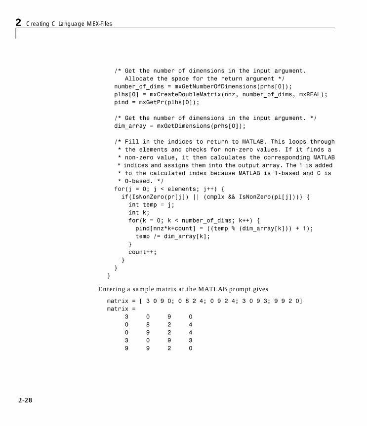
2 Creating C Language MEX-Files
2-28
/* Get the number of dimensions in the input argument. Allocate the space for the return argument */ number_of_dims = mxGetNumberOfDimensions(prhs[0]); plhs[0] = mxCreateDoubleMatrix(nnz, number_of_dims, mxREAL); pind = mxGetPr(plhs[0]);
/* Get the number of dimensions in the input argument. */ dim_array = mxGetDimensions(prhs[0]);
/* Fill in the indices to return to MATLAB. This loops through * the elements and checks for non-zero values. If it finds a * non-zero value, it then calculates the corresponding MATLAB * indices and assigns them into the output array. The 1 is added * to the calculated index because MATLAB is 1-based and C is * 0-based. */ for(j = 0; j < elements; j++) { if(IsNonZero(pr[j]) || (cmplx && IsNonZero(pi[j]))) { int temp = j; int k; for(k = 0; k < number_of_dims; k++) { pind[nnz*k+count] = ((temp % (dim_array[k])) + 1); temp /= dim_array[k]; } count++; } }}
Entering a sample matrix at the MATLAB prompt gives
matrix = [ 3 0 9 0; 0 8 2 4; 0 9 2 4; 3 0 9 3; 9 9 2 0]matrix = 3 0 9 0 0 8 2 4 0 9 2 4 3 0 9 3 9 9 2 0
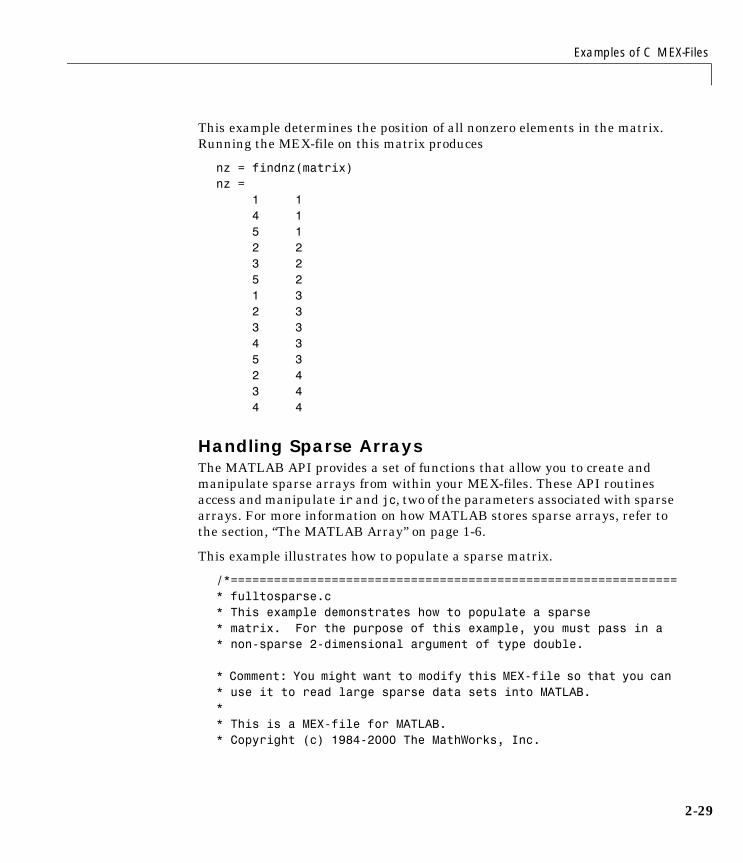
Examples of C MEX-Files
2-29
This example determines the position of all nonzero elements in the matrix. Running the MEX-file on this matrix produces
nz = findnz(matrix)nz = 1 1 4 1 5 1 2 2 3 2 5 2 1 3 2 3 3 3 4 3 5 3 2 4 3 4 4 4
Handling Sparse ArraysThe MATLAB API provides a set of functions that allow you to create and manipulate sparse arrays from within your MEX-files. These API routines access and manipulate ir and jc, two of the parameters associated with sparse arrays. For more information on how MATLAB stores sparse arrays, refer to the section, “The MATLAB Array” on page 1-6.
This example illustrates how to populate a sparse matrix.
/*==============================================================* fulltosparse.c* This example demonstrates how to populate a sparse* matrix. For the purpose of this example, you must pass in a* non-sparse 2-dimensional argument of type double.
* Comment: You might want to modify this MEX-file so that you can * use it to read large sparse data sets into MATLAB.** This is a MEX-file for MATLAB. * Copyright (c) 1984-2000 The MathWorks, Inc.
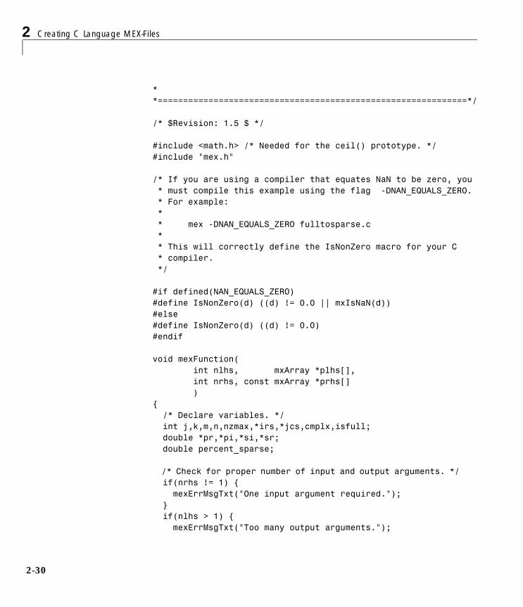
2 Creating C Language MEX-Files
2-30
* *=============================================================*/
/* $Revision: 1.5 $ */
#include <math.h> /* Needed for the ceil() prototype. */#include "mex.h"
/* If you are using a compiler that equates NaN to be zero, you * must compile this example using the flag -DNAN_EQUALS_ZERO. * For example: * * mex -DNAN_EQUALS_ZERO fulltosparse.c * * This will correctly define the IsNonZero macro for your C * compiler. */
#if defined(NAN_EQUALS_ZERO)#define IsNonZero(d) ((d) != 0.0 || mxIsNaN(d))#else#define IsNonZero(d) ((d) != 0.0)#endif
void mexFunction( int nlhs, mxArray *plhs[], int nrhs, const mxArray *prhs[] ){ /* Declare variables. */ int j,k,m,n,nzmax,*irs,*jcs,cmplx,isfull; double *pr,*pi,*si,*sr; double percent_sparse;
/* Check for proper number of input and output arguments. */ if(nrhs != 1) { mexErrMsgTxt("One input argument required."); } if(nlhs > 1) { mexErrMsgTxt("Too many output arguments.");
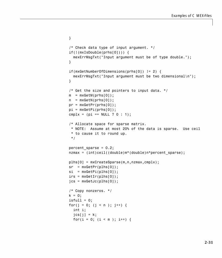
Examples of C MEX-Files
2-31
}
/* Check data type of input argument. */ if(!(mxIsDouble(prhs[0]))) { mexErrMsgTxt("Input argument must be of type double."); }
if(mxGetNumberOfDimensions(prhs[0]) != 2) { mexErrMsgTxt("Input argument must be two dimensional\n"); }
/* Get the size and pointers to input data. */ m = mxGetM(prhs[0]); n = mxGetN(prhs[0]); pr = mxGetPr(prhs[0]); pi = mxGetPi(prhs[0]); cmplx = (pi == NULL ? 0 : 1);
/* Allocate space for sparse matrix. * NOTE: Assume at most 20% of the data is sparse. Use ceil * to cause it to round up. */
percent_sparse = 0.2; nzmax = (int)ceil((double)m*(double)n*percent_sparse);
plhs[0] = mxCreateSparse(m,n,nzmax,cmplx); sr = mxGetPr(plhs[0]); si = mxGetPi(plhs[0]); irs = mxGetIr(plhs[0]); jcs = mxGetJc(plhs[0]); /* Copy nonzeros. */ k = 0; isfull = 0; for(j = 0; (j < n ); j++) { int i; jcs[j] = k; for(i = 0; (i < m ); i++) {

2 Creating C Language MEX-Files
2-32
if(IsNonZero(pr[i]) || (cmplx && IsNonZero(pi[i]))) {
/* Check to see if non-zero element will fit in * allocated output array. If not, increase * percent_sparse by 10%, recalculate nzmax, and augment * the sparse array. */ if(k >= nzmax) { int oldnzmax = nzmax; percent_sparse += 0.1; nzmax = (int)ceil((double)m*(double)n*percent_sparse);
/* Make sure nzmax increases atleast by 1. */ if(oldnzmax == nzmax) nzmax++;
mxSetNzmax(plhs[0], nzmax); mxSetPr(plhs[0], mxRealloc(sr, nzmax*sizeof(double))); if(si != NULL) mxSetPi(plhs[0], mxRealloc(si, nzmax*sizeof(double))); mxSetIr(plhs[0], mxRealloc(irs, nzmax*sizeof(int)));
sr = mxGetPr(plhs[0]); si = mxGetPi(plhs[0]); irs = mxGetIr(plhs[0]); } sr[k] = pr[i]; if(cmplx) { si[k] = pi[i]; } irs[k] = i; k++; } } pr += m; pi += m; } jcs[n] = k;}
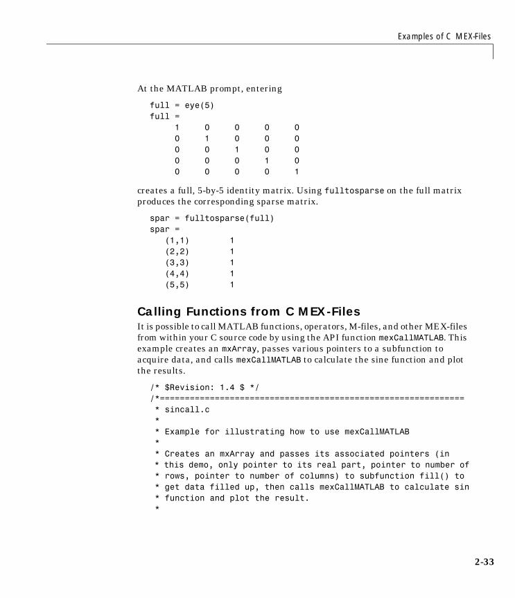
Examples of C MEX-Files
2-33
At the MATLAB prompt, entering
full = eye(5)full = 1 0 0 0 0 0 1 0 0 0 0 0 1 0 0 0 0 0 1 0 0 0 0 0 1
creates a full, 5-by-5 identity matrix. Using fulltosparse on the full matrix produces the corresponding sparse matrix.
spar = fulltosparse(full)spar = (1,1) 1 (2,2) 1 (3,3) 1 (4,4) 1 (5,5) 1
Calling Functions from C MEX-FilesIt is possible to call MATLAB functions, operators, M-files, and other MEX-files from within your C source code by using the API function mexCallMATLAB. This example creates an mxArray, passes various pointers to a subfunction to acquire data, and calls mexCallMATLAB to calculate the sine function and plot the results.
/* $Revision: 1.4 $ *//*============================================================= * sincall.c * * Example for illustrating how to use mexCallMATLAB * * Creates an mxArray and passes its associated pointers (in * this demo, only pointer to its real part, pointer to number of * rows, pointer to number of columns) to subfunction fill() to * get data filled up, then calls mexCallMATLAB to calculate sin * function and plot the result. *
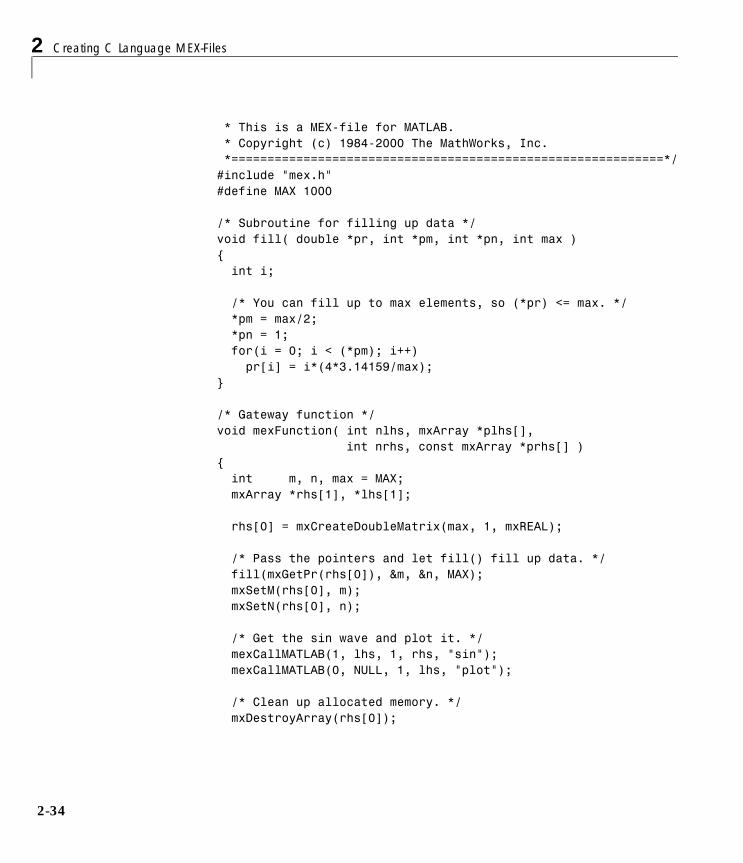
2 Creating C Language MEX-Files
2-34
* This is a MEX-file for MATLAB. * Copyright (c) 1984-2000 The MathWorks, Inc. *============================================================*/#include "mex.h"#define MAX 1000
/* Subroutine for filling up data */void fill( double *pr, int *pm, int *pn, int max ){ int i;
/* You can fill up to max elements, so (*pr) <= max. */ *pm = max/2; *pn = 1; for(i = 0; i < (*pm); i++) pr[i] = i*(4*3.14159/max);}
/* Gateway function */void mexFunction( int nlhs, mxArray *plhs[], int nrhs, const mxArray *prhs[] ){ int m, n, max = MAX; mxArray *rhs[1], *lhs[1]; rhs[0] = mxCreateDoubleMatrix(max, 1, mxREAL); /* Pass the pointers and let fill() fill up data. */ fill(mxGetPr(rhs[0]), &m, &n, MAX); mxSetM(rhs[0], m); mxSetN(rhs[0], n); /* Get the sin wave and plot it. */ mexCallMATLAB(1, lhs, 1, rhs, "sin"); mexCallMATLAB(0, NULL, 1, lhs, "plot"); /* Clean up allocated memory. */ mxDestroyArray(rhs[0]);
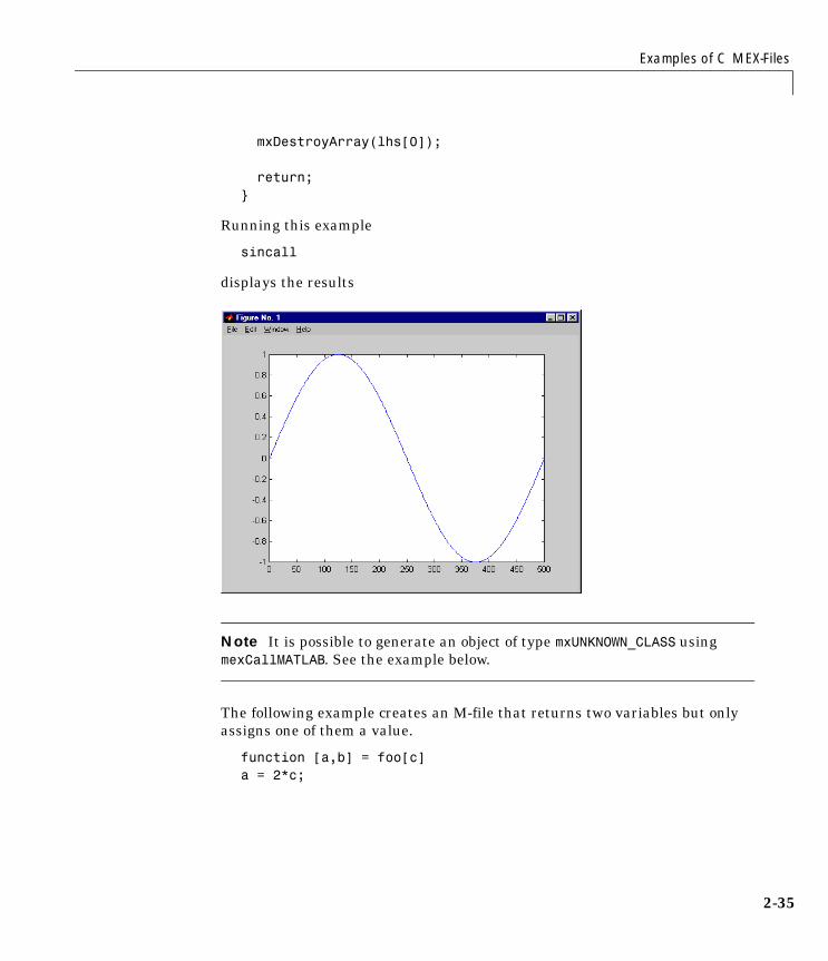
Examples of C MEX-Files
2-35
mxDestroyArray(lhs[0]); return;}
Running this example
sincall
displays the results
Note It is possible to generate an object of type mxUNKNOWN_CLASS using mexCallMATLAB. See the example below.
The following example creates an M-file that returns two variables but only assigns one of them a value.
function [a,b] = foo[c]a = 2*c;
2 Creating C Language MEX-Files
2-36
MATLAB displays the following warning message.
Warning: One or more output arguments not assigned during call to 'foo'.
If you then call foo using mexCallMATLAB, the unassigned output variable will now be of type mxUNKNOWN_CLASS.
Advanced Topics
2-37
Advanced TopicsThese sections cover advanced features of MEX-files that you can use when your applications require sophisticated MEX-files.
Help Files• Because the MATLAB interpreter chooses the MEX-file when both an M-file
and a MEX-file with the same name are encountered in the same directory, it is possible to use M-files for documenting the behavior of your MEX-files. The MATLAB help command will automatically find and display the appropriate M-file when help is requested and the interpreter will find and execute the corresponding MEX-file when the function is invoked.
Linking Multiple FilesIt is possible to combine several object files and to use object file libraries when building MEX-files. To do so, simply list the additional files with their full extension, separated by spaces. For example, on the PC
mex circle.c square.obj rectangle.c shapes.lib
is a legal command that operates on the .c, .obj, and .lib files to create a MEX-file called circle.dll, where dll is the extension corresponding to the MEX-file type on the PC. The name of the resulting MEX-file is taken from the first file in the list.
You may find it useful to use a software development tool like MAKE to manage MEX-file projects involving multiple source files. Simply create a MAKEFILE that contains a rule for producing object files from each of your source files and then invoke mex to combine your object files into a MEX-file. This way you can ensure that your source files are recompiled only when necessary.
Workspace for MEX-File FunctionsUnlike M-file functions, MEX-file functions do not have their own variable workspace. MEX-file functions operate in the caller’s workspace.
mexEvalString evaluates the string in the caller’s workspace. In addition, you can use the mexGetArray and mexPutArray routines to get and put variables into the caller’s workspace.

2 Creating C Language MEX-Files
2-38
Memory ManagementMemory management within MEX-files is not unlike memory management for regular C or Fortran applications. However, there are special considerations because the MEX-file must exist within the context of a larger application, i.e., MATLAB itself.
Automatic Cleanup of Temporary ArraysWhen a MEX-file returns to MATLAB, it gives to MATLAB the results of its computations in the form of the left-hand side arguments – the mxArrays contained within the plhs[] list. Any mxArrays created by the MEX-file that are not in this list are automatically destroyed. In addition, any memory allocated with mxCalloc, mxMalloc, or mxRealloc during the MEX-file’s execution is automatically freed.
In general, we recommend that MEX-files destroy their own temporary arrays and free their own dynamically allocated memory. It is more efficient for the MEX-file to perform this cleanup than to rely on the automatic mechanism. However, there are several circumstances in which the MEX-file will not reach its normal return statement. The normal return will not be reached if:
• A call to mexErrMsgTxt occurs.
• A call to mexCallMATLAB occurs and the function being called creates an error. (A MEX-file can trap such errors by using mexSetTrapFlag, but not all MEX-files would necessarily need to trap errors.)
• The user interrupts the MEX-file’s execution using Ctrl-C.
• The MEX-file runs out of memory. When this happens, MATLAB’s out-of-memory handler will immediately terminate the MEX-file.
A careful MEX-file programmer can ensure safe cleanup of all temporary arrays and memory before returning in the first two cases, but not in the last two cases. In the last two cases, the automatic cleanup mechanism is necessary to prevent memory leaks.
Persistent ArraysYou can exempt an array, or a piece of memory, from MATLAB’s automatic cleanup by calling mexMakeArrayPersistent or mexMakeMemoryPersistent. However, if a MEX-file creates such persistent objects, there is a danger that a memory leak could occur if the MEX-file is cleared before the persistent object is properly destroyed. In order to prevent this from happening, a MEX-file that
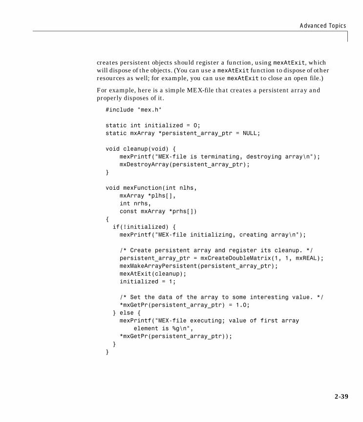
Advanced Topics
2-39
creates persistent objects should register a function, using mexAtExit, which will dispose of the objects. (You can use a mexAtExit function to dispose of other resources as well; for example, you can use mexAtExit to close an open file.)
For example, here is a simple MEX-file that creates a persistent array and properly disposes of it.
#include "mex.h"
static int initialized = 0;static mxArray *persistent_array_ptr = NULL;
void cleanup(void) { mexPrintf("MEX-file is terminating, destroying array\n"); mxDestroyArray(persistent_array_ptr);}
void mexFunction(int nlhs, mxArray *plhs[], int nrhs, const mxArray *prhs[]){ if(!initialized) { mexPrintf("MEX-file initializing, creating array\n"); /* Create persistent array and register its cleanup. */ persistent_array_ptr = mxCreateDoubleMatrix(1, 1, mxREAL); mexMakeArrayPersistent(persistent_array_ptr); mexAtExit(cleanup); initialized = 1;
/* Set the data of the array to some interesting value. */ *mxGetPr(persistent_array_ptr) = 1.0; } else { mexPrintf("MEX-file executing; value of first array element is %g\n", *mxGetPr(persistent_array_ptr)); }}
2 Creating C Language MEX-Files
2-40
Hybrid ArraysFunctions such as mxSetPr, mxSetData, and mxSetCell allow the direct placement of memory pieces into an mxArray. mxDestroyArray will destroy these pieces along with the entire array. Because of this, it is possible to create an array that cannot be destroyed, i.e., an array on which it is not safe to call mxDestroyArray. Such an array is called a hybrid array, because it contains both destroyable and nondestroyable components.
For example, it is not legal to call mxFree (or the ANSI free() function, for that matter) on automatic variables. Therefore, in the following code fragment, pArray is a hybrid array.
mxArray *pArray = mxCreateDoubleMatrix(0, 0, mxREAL);double data[10];
mxSetPr(pArray, data);mxSetM(pArray, 1);mxSetN(pArray, 10);
Another example of a hybrid array is a cell array or structure, one of whose children is a read-only array (an array with the const qualifier, such as one of the inputs to the MEX-file). The array cannot be destroyed because the input to the MEX-file would also be destroyed.
Because hybrid arrays cannot be destroyed, they cannot be cleaned up by the automatic mechanism outlined in “Automatic Cleanup of Temporary Arrays” on page 2-38. As described in that section, the automatic cleanup mechanism is the only way to destroy temporary arrays in case of a user interrupt. Therefore, temporary hybrid arrays are illegal and may cause your MEX-file to crash.
Although persistent hybrid arrays are viable, we recommend avoiding their use wherever possible.
Using LAPACK and BLAS FunctionsLAPACK is a large, multiauthor Fortran subroutine library that MATLAB uses for numerical linear algebra. BLAS, which stands for Basic Linear Algebra Subroutines, is used by MATLAB to speed up matrix multiplication and the LAPACK routines themselves. The functions provided by LAPACK and BLAS can also be called directly from within your C MEX-files.
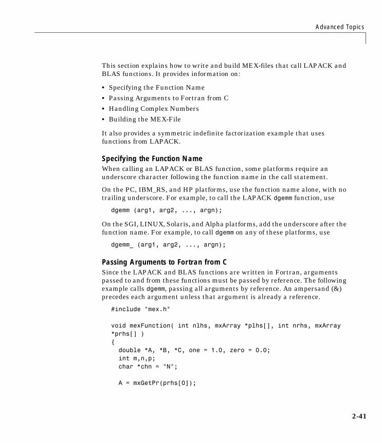
Advanced Topics
2-41
This section explains how to write and build MEX-files that call LAPACK and BLAS functions. It provides information on:
• Specifying the Function Name
• Passing Arguments to Fortran from C
• Handling Complex Numbers
• Building the MEX-File
It also provides a symmetric indefinite factorization example that uses functions from LAPACK.
Specifying the Function NameWhen calling an LAPACK or BLAS function, some platforms require an underscore character following the function name in the call statement.
On the PC, IBM_RS, and HP platforms, use the function name alone, with no trailing underscore. For example, to call the LAPACK dgemm function, use
dgemm (arg1, arg2, ..., argn);
On the SGI, LINUX, Solaris, and Alpha platforms, add the underscore after the function name. For example, to call dgemm on any of these platforms, use
dgemm_ (arg1, arg2, ..., argn);
Passing Arguments to Fortran from CSince the LAPACK and BLAS functions are written in Fortran, arguments passed to and from these functions must be passed by reference. The following example calls dgemm, passing all arguments by reference. An ampersand (&) precedes each argument unless that argument is already a reference.
#include "mex.h"
void mexFunction( int nlhs, mxArray *plhs[], int nrhs, mxArray *prhs[] ){ double *A, *B, *C, one = 1.0, zero = 0.0; int m,n,p; char *chn = "N";
A = mxGetPr(prhs[0]);
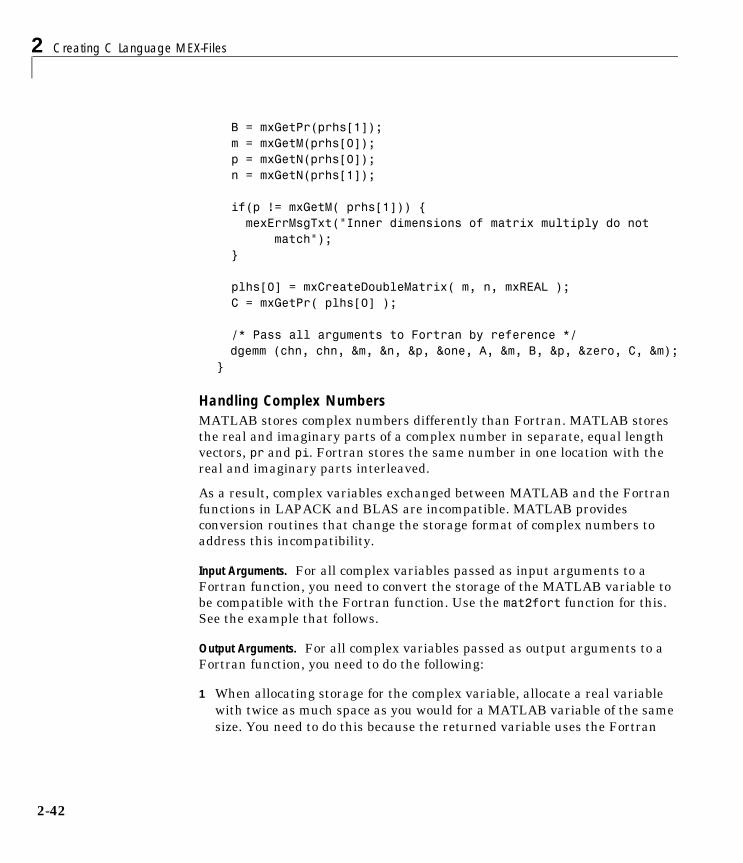
2 Creating C Language MEX-Files
2-42
B = mxGetPr(prhs[1]); m = mxGetM(prhs[0]); p = mxGetN(prhs[0]); n = mxGetN(prhs[1]);
if(p != mxGetM( prhs[1])) { mexErrMsgTxt("Inner dimensions of matrix multiply do not match"); }
plhs[0] = mxCreateDoubleMatrix( m, n, mxREAL ); C = mxGetPr( plhs[0] );
/* Pass all arguments to Fortran by reference */ dgemm (chn, chn, &m, &n, &p, &one, A, &m, B, &p, &zero, C, &m);}
Handling Complex NumbersMATLAB stores complex numbers differently than Fortran. MATLAB stores the real and imaginary parts of a complex number in separate, equal length vectors, pr and pi. Fortran stores the same number in one location with the real and imaginary parts interleaved.
As a result, complex variables exchanged between MATLAB and the Fortran functions in LAPACK and BLAS are incompatible. MATLAB provides conversion routines that change the storage format of complex numbers to address this incompatibility.
Input Arguments. For all complex variables passed as input arguments to a Fortran function, you need to convert the storage of the MATLAB variable to be compatible with the Fortran function. Use the mat2fort function for this. See the example that follows.
Output Arguments. For all complex variables passed as output arguments to a Fortran function, you need to do the following:
1 When allocating storage for the complex variable, allocate a real variable with twice as much space as you would for a MATLAB variable of the same size. You need to do this because the returned variable uses the Fortran
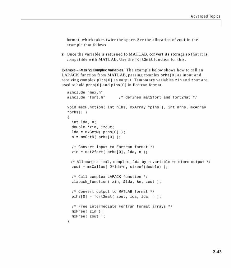
Advanced Topics
2-43
format, which takes twice the space. See the allocation of zout in the example that follows.
2 Once the variable is returned to MATLAB, convert its storage so that it is compatible with MATLAB. Use the fort2mat function for this.
Example – Passing Complex Variables. The example below shows how to call an LAPACK function from MATLAB, passing complex prhs[0] as input and receiving complex plhs[0] as output. Temporary variables zin and zout are used to hold prhs[0] and plhs[0] in Fortran format.
#include "mex.h" #include "fort.h" /* defines mat2fort and fort2mat */
void mexFunction( int nlhs, mxArray *plhs[], int nrhs, mxArray *prhs[] ) { int lda, n; double *zin, *zout; lda = mxGetM( prhs[0] ); n = mxGetN( prhs[0] );
/* Convert input to Fortran format */ zin = mat2fort( prhs[0], lda, n );
/* Allocate a real, complex, lda-by-n variable to store output */ zout = mxCalloc( 2*lda*n, sizeof(double) );
/* Call complex LAPACK function */ zlapack_function( zin, &lda, &n, zout );
/* Convert output to MATLAB format */ plhs[0] = fort2mat( zout, lda, lda, n );
/* Free intermediate Fortran format arrays */ mxFree( zin ); mxFree( zout ); }
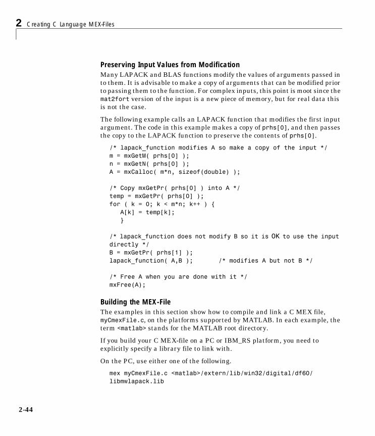
2 Creating C Language MEX-Files
2-44
Preserving Input Values from ModificationMany LAPACK and BLAS functions modify the values of arguments passed in to them. It is advisable to make a copy of arguments that can be modified prior to passing them to the function. For complex inputs, this point is moot since the mat2fort version of the input is a new piece of memory, but for real data this is not the case.
The following example calls an LAPACK function that modifies the first input argument. The code in this example makes a copy of prhs[0], and then passes the copy to the LAPACK function to preserve the contents of prhs[0].
/* lapack_function modifies A so make a copy of the input */ m = mxGetM( prhs[0] ); n = mxGetN( prhs[0] ); A = mxCalloc( m*n, sizeof(double) );
/* Copy mxGetPr( prhs[0] ) into A */ temp = mxGetPr( prhs[0] ); for ( k = 0; k < m*n; k++ ) { A[k] = temp[k]; }
/* lapack_function does not modify B so it is OK to use the input directly */ B = mxGetPr( prhs[1] );lapack_function( A,B ); /* modifies A but not B */
/* Free A when you are done with it */ mxFree(A);
Building the MEX-FileThe examples in this section show how to compile and link a C MEX file, myCmexFile.c, on the platforms supported by MATLAB. In each example, the term <matlab> stands for the MATLAB root directory.
If you build your C MEX-file on a PC or IBM_RS platform, you need to explicitly specify a library file to link with.
On the PC, use either one of the following.
mex myCmexFile.c <matlab>/extern/lib/win32/digital/df60/libmwlapack.lib
Advanced Topics
2-45
mex myCmexFile.c <matlab>/extern/lib/win32/microsoft/msvc60/libmwlapack.lib
For IBM_RS, use the following syntax.
mex myCmexFile.c -L<matlab>/bin/ibm_rs -lmwlapack
On all other platforms, you can build your MEX-file as you would any other C MEX-file. For example,
mex myCmexFile.c
MEX-Files That Perform Complex Number Conversion. MATLAB supplies the files fort.c and fort.h, which provide routines for conversion between MATLAB and FORTRAN complex data structures. These files define the mat2fort and fort2mat routines mentioned previously under “Handling Complex Numbers” on page 2-42.
If your program uses these routines, then you need to:
1 Include the fort.h file in your program, using, #include "fort.h". See the example above.
2 Build the fort.c file with your program. Specify the pathname, <matlab>/extern/examples/refbook for both fort.c and fort.h in the build command, (where <matlab> stands for the MATLAB root directory).
On the PC, use either one of the following.
mex myCmexFile.c <matlab>/extern/examples/refbook/fort.c -I<matlab>/extern/examples/refbook <matlab>/extern/lib/win32/digital/df60/libmwlapack.lib
mex myCmexFile.c <matlab>/extern/examples/refbook/fort.c -I<matlab>/extern/examples/refbook <matlab>/extern/lib/win32/microsoft/msvc60/libmwlapack.lib
For IBM_RS, use
mex myCmexFile.c <matlab>/extern/examples/refbook/fort.c -I<matlab>/extern/examples/refbook -L<matlab>/bin/ibm_rs -lmwlapack
For all other platforms, use
2 Creating C Language MEX-Files
2-46
mex myCmexFile.c <matlab>/extern/examples/refbook/fort.c -I<matlab>/extern/examples/refbook
Example – Symmetric Indefinite Factorization Using LAPACKYou will find an example C MEX-file that calls two LAPACK functions in the directory <matlab>/extern/examples/refbook, where <matlab> stands for the MATLAB root directory. There are two versions of this file:
• utdu_slv.c – calls functions zhesvx and dsysvx, and thus is compatible with the PC, HP, and IBM platforms.
• utdu_slv_.c – calls functions zhesvx_ and dsysvx_, and thus is compatible with the SGI, LINUX, Solaris, and Alpha platforms.
Debugging C Language MEX-Files
2-47
Debugging C Language MEX-FilesOn most platforms, it is now possible to debug MEX-files while they are running within MATLAB. Complete source code debugging, including setting breakpoints, examining variables, and stepping through the source code line-by-line, is now available.
Note The section entitled, “Troubleshooting” on page 1-32, provides additional information on isolating problems with MEX-files.
To debug a MEX-file from within MATLAB, you must first compile the MEX-file with the -g option to mex.
mex -g filename.c
Debugging on UNIXYou need to start MATLAB from within a debugger. To do this, specify the name of the debugger you want to use with the -D option when starting MATLAB.
This example shows how to debug yprime.c on Solaris using dbx, the UNIX debugger.
unix> mex -g yprime.cunix> matlab -Ddbx<dbx> stop dlopen <matlab>/extern/examples/mex/yprime.mexsol
Once the debugger loads MATLAB into memory, you can start it by issuing a run command.
<dbx> run
Now, run the MEX-file that you want to debug as you would ordinarily do (either directly or by means of some other function or script). Before executing the MEX-file, you will be returned to the debugger.
>> yprime(1,1:4)<dbx> stop in ‘yprime.mexsol‘mexFunction
2 Creating C Language MEX-Files
2-48
Note The tick marks used are back ticks (‘), not single quotes (').
You may need to tell the debugger where the MEX-file was loaded or the name of the MEX-file, in which case MATLAB will display the appropriate command for you to use. At this point, you are ready to start debugging. You can list the source code for your MEX-file and set breakpoints in it. It is often convenient to set one at mexFunction so that you stop at the beginning of the gateway routine. To proceed from the breakpoint, issue a continue command to the debugger.
<dbx> cont
Once you hit one of your breakpoints, you can make full use of any facilities that your debugger provides to examine variables, display memory, or inspect registers. Refer to the documentation provided with your debugger for information on its use.
Note For information on debugging on other UNIX platforms, access the MathWorks Technical Support Web site at http://www.mathworks.com/support.
Debugging on WindowsThe following sections provide instructions on how to debug on Microsoft Windows systems using various compilers.
Microsoft CompilerIf you are using the Microsoft compiler:
1 Start the Microsoft Visual Studio (Version 5 or 6) by typing at the DOS prompt
msdev filename.dll
2 In the Microsoft environment, from the Project menu, select Settings. In the window that opens, select the Debug tab. This options window contains
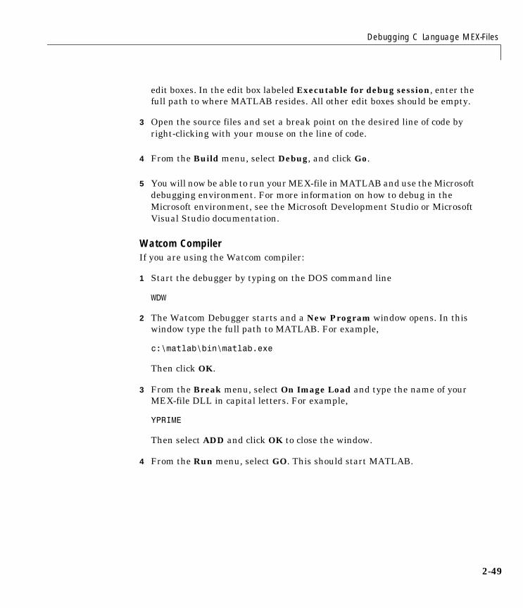
Debugging C Language MEX-Files
2-49
edit boxes. In the edit box labeled Executable for debug session, enter the full path to where MATLAB resides. All other edit boxes should be empty.
3 Open the source files and set a break point on the desired line of code by right-clicking with your mouse on the line of code.
4 From the Build menu, select Debug, and click Go.
5 You will now be able to run your MEX-file in MATLAB and use the Microsoft debugging environment. For more information on how to debug in the Microsoft environment, see the Microsoft Development Studio or Microsoft Visual Studio documentation.
Watcom CompilerIf you are using the Watcom compiler:
1 Start the debugger by typing on the DOS command line
WDW
2 The Watcom Debugger starts and a New Program window opens. In this window type the full path to MATLAB. For example,
c:\matlab\bin\matlab.exe
Then click OK.
3 From the Break menu, select On Image Load and type the name of your MEX-file DLL in capital letters. For example,
YPRIME
Then select ADD and click OK to close the window.
4 From the Run menu, select GO. This should start MATLAB.
2 Creating C Language MEX-Files
2-50
5 When MATLAB starts, in the command window change directories to where your MEX-file resides and run your MEX-file. If a message similar to the following appears, ignore the message and click OK.
LDR: Automatic DLL Relocation in matlab.exeLDR: DLL filename.dll base <number> relocated due to collision with matlab.exe
6 Open the file you want to debug and set breakpoints in the source code.
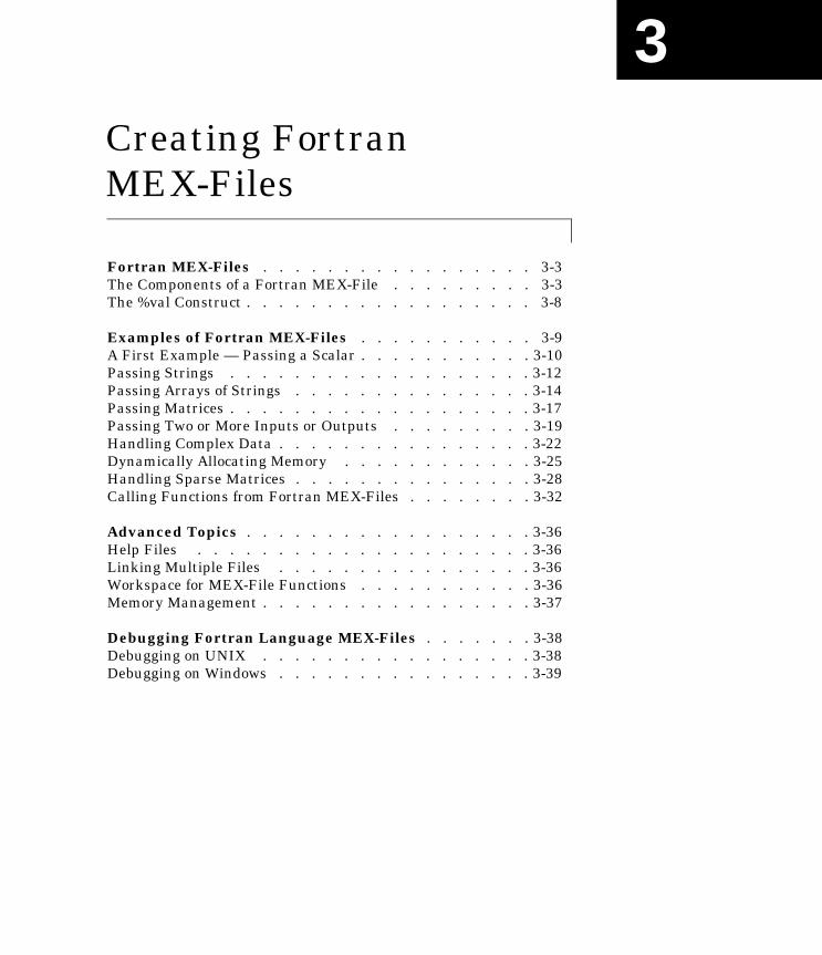
3Creating Fortran MEX-Files
Fortran MEX-Files . . . . . . . . . . . . . . . . . 3-3The Components of a Fortran MEX-File . . . . . . . . . 3-3The %val Construct . . . . . . . . . . . . . . . . . . 3-8
Examples of Fortran MEX-Files . . . . . . . . . . . 3-9A First Example — Passing a Scalar . . . . . . . . . . . 3-10Passing Strings . . . . . . . . . . . . . . . . . . . 3-12Passing Arrays of Strings . . . . . . . . . . . . . . . 3-14Passing Matrices . . . . . . . . . . . . . . . . . . . 3-17Passing Two or More Inputs or Outputs . . . . . . . . . 3-19Handling Complex Data . . . . . . . . . . . . . . . . 3-22Dynamically Allocating Memory . . . . . . . . . . . . 3-25Handling Sparse Matrices . . . . . . . . . . . . . . . 3-28Calling Functions from Fortran MEX-Files . . . . . . . . 3-32
Advanced Topics . . . . . . . . . . . . . . . . . . 3-36Help Files . . . . . . . . . . . . . . . . . . . . . 3-36Linking Multiple Files . . . . . . . . . . . . . . . . 3-36Workspace for MEX-File Functions . . . . . . . . . . . 3-36Memory Management . . . . . . . . . . . . . . . . . 3-37
Debugging Fortran Language MEX-Files . . . . . . . 3-38Debugging on UNIX . . . . . . . . . . . . . . . . . 3-38Debugging on Windows . . . . . . . . . . . . . . . . 3-39
3 Creating Fortran MEX-Files
3-2
This chapter describes how to write MEX-files in the Fortran programming language. It discusses the MEX-file itself, how these Fortran language files interact with MATLAB, how to pass and manipulate arguments of different data types, how to debug your MEX-file programs, and several other, more advanced topics.
The following list summarizes the contents of this chapter:
• “Fortran MEX-Files”
• “Examples of Fortran MEX-Files”
• “Advanced Topics”
• “Debugging Fortran Language MEX-Files”
Fortran MEX-Files
3-3
Fortran MEX-FilesFortran MEX-files are built by using the mex script to compile your Fortran source code with additional calls to API routines.
MEX-files in Fortran can only create double-precision data and strings, unlike their C counterparts, which can create any data type supported by MATLAB. You can treat Fortran MEX-files, once compiled, exactly like M-functions.
The Components of a Fortran MEX-FileThis section discusses the specific elements needed in a Fortran MEX-file. The source code for a Fortran MEX-file, like the C MEX-file, consists of two distinct parts:
• A computational routine that contains the code for performing the computations that you want implemented in the MEX-file. Computations can be numerical computations as well as inputting and outputting data.
• A gateway routine that interfaces the computational routine with MATLAB by the entry point mexFunction and its parameters prhs, nrhs, plhs, nlhs, where prhs is an array of right-hand input arguments, nrhs is the number of right-hand input arguments, plhs is an array of left-hand output arguments, and nlhs is the number of left-hand output arguments. The gateway calls the computational routine as a subroutine.
The computational and gateway routines may be separate or combined. The following figure, Fortran MEX Cycle, shows how inputs enter an API function, what functions the gateway routine performs, and how output returns to MATLAB.
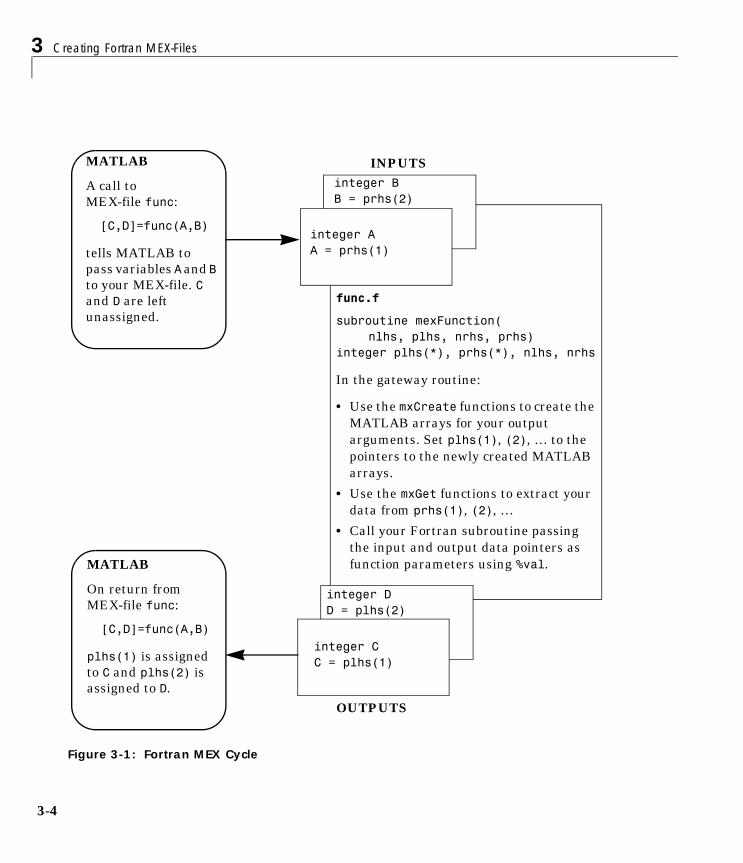
3 Creating Fortran MEX-Files
3-4
Figure 3-1: Fortran MEX Cycle
integer AA = prhs(1)
MATLAB
A call to MEX-file func:
[C,D]=func(A,B)
tells MATLAB to pass variables A and B to your MEX-file. C and D are left unassigned.
integer CC = plhs(1)
integer BB = prhs(2)
integer DD = plhs(2)
INPUTS
OUTPUTS
func.f
subroutine mexFunction(nlhs, plhs, nrhs, prhs)
integer plhs(*), prhs(*), nlhs, nrhs
In the gateway routine:
• Use the mxCreate functions to create the MATLAB arrays for your output arguments. Set plhs(1), (2), … to the pointers to the newly created MATLAB arrays.
• Use the mxGet functions to extract your data from prhs(1), (2), …
• Call your Fortran subroutine passing the input and output data pointers as function parameters using %val.MATLAB
On return fromMEX-file func:
[C,D]=func(A,B)
plhs(1) is assigned to C and plhs(2) is assigned to D.
Fortran MEX-Files
3-5
The Pointer ConceptThe MATLAB API works with a unique data type, the mxArray. Because there is no way to create a new data type in Fortran, MATLAB passes a special identifier, called a pointer, to a Fortran program. You can get information about an mxArray by passing this pointer to various API functions called Access Routines. These access routines allow you to get a native Fortran data type containing exactly the information you want, i.e., the size of the mxArray, whether or not it is a string, or its data contents.
There are several implications when using pointers in Fortran:
• The %val construct.
If your Fortran compiler supports the %val construct, then there is one type of pointer you can use without requiring an access routine, namely a pointer to data (i.e., the pointer returned by mxGetPr or mxGetPi). You can use %val to pass this pointer’s contents to a subroutine, where it is declared as a Fortran double-precision matrix.
If your Fortran compiler does not support the %val construct, you must use the mxCopy__ routines (e.g., mxCopyPtrToReal8) to access the contents of the pointer. For more information about the %val construct and an example, see the section, “The %val Construct” on page 3-8.
• Variable declarations.
To use pointers properly, you must declare them to be the correct size. On DEC Alpha machines, all pointers should be declared as integer*8. On all other platforms, pointers should be declared as integer*4.
If your Fortran compiler supports preprocessing with the C preprocessor, you can use the preprocessing stage to map pointers to the appropriate declaration. In UNIX, see the examples ending with .F in the examples directory for a possible approach.
Caution Declaring a pointer to be the incorrect size may cause your program to crash.
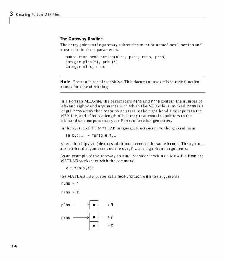
3 Creating Fortran MEX-Files
3-6
The Gateway RoutineThe entry point to the gateway subroutine must be named mexFunction and must contain these parameters.
subroutine mexFunction(nlhs, plhs, nrhs, prhs)integer plhs(*), prhs(*)integer nlhs, nrhs
Note Fortran is case-insensitive. This document uses mixed-case function names for ease of reading.
In a Fortran MEX-file, the parameters nlhs and nrhs contain the number of left- and right-hand arguments with which the MEX-file is invoked. prhs is a length nrhs array that contains pointers to the right-hand side inputs to the MEX-file, and plhs is a length nlhs array that contains pointers to the left-hand side outputs that your Fortran function generates.
In the syntax of the MATLAB language, functions have the general form
[a,b,c,…] = fun(d,e,f,…)
where the ellipsis (…) denotes additional terms of the same format. The a,b,c,… are left-hand arguments and the d,e,f,… are right-hand arguments.
As an example of the gateway routine, consider invoking a MEX-file from the MATLAB workspace with the command
x = fun(y,z);
the MATLAB interpreter calls mexFunction with the arguments
nlhs = 1
nrhs = 2
plhs
prhs
• Ø
• Y
• Z
Fortran MEX-Files
3-7
plhs is a 1-element C array where the single element is a null pointer. prhs is a 2-element C array where the first element is a pointer to an mxArray named Y and the second element is a pointer to an mxArray named Z.
The parameter plhs points at nothing because the output x is not created until the subroutine executes. It is the responsibility of the gateway routine to create an output array and to set a pointer to that array in plhs(1). If plhs(1) is left unassigned, MATLAB prints a warning message stating that no output has been assigned.
Note It is possible to return an output value even if nlhs = 0. This corresponds to returning the result in the ans variable.
The gateway routine should validate the input arguments and call mexErrMsgTxt if anything is amiss. This step includes checking the number, type, and size of the input arrays as well as examining the number of output arrays. The examples included later in this section illustrate this technique.
The mx functions provide a set of access methods (subroutines) for manipulating MATLAB arrays. These functions are fully documented in the online API reference pages. The mx prefix is shorthand for mxArray and it means that the function enables you to access and/or manipulate some of the information in the MATLAB array. For example, mxGetPr gets the real data from the MATLAB array. Additional routines are provided for transferring data between MATLAB arrays and Fortran arrays.
The gateway routine must call mxCreateFull, mxCreateSparse, or mxCreateString to create MATLAB arrays of the required sizes in which to return the results. The return values from these calls should be assigned to the appropriate elements of plhs.
The gateway routine may call mxCalloc to allocate temporary work arrays for the computational routine if it needs them.
The gateway routine should call the computational routine to perform the desired calculations or operations. There are a number of additional routines that MEX-files can use. These routines are distinguished by the initial characters mex, as in mexCallMATLAB and mexErrMsgTxt.
3 Creating Fortran MEX-Files
3-8
When a MEX-file completes its task, it returns control to MATLAB. Any MATLAB arrays that are created by the MEX-file that are not returned to MATLAB through the left-hand side arguments are automatically destroyed.
The %val ConstructThe %val construct is supported by most, but not all, Fortran compilers. DIGITAL Visual Fortran does support the construct. %val causes the value of the variable, rather than the address of the variable, to be passed to the subroutine. If you are using a Fortran compiler that does not support the %val construct, you must copy the array values into a temporary true Fortran array using special routines. For example, consider a gateway routine that calls its computational routine, yprime, by
call yprime(%val(yp), %val(t), %val(y))
If your Fortran compiler does not support the %val construct, you would replace the call to the computational subroutine with
C Copy array pointers to local arrays.call mxCopyPtrToReal8(t, tr, 1)call mxCopyPtrToReal8(y, yr, 4)
CC Call the computational subroutine.
call yprime(ypr, tr, yr)CC Copy local array to output array pointer.
call mxCopyReal8ToPtr(ypr, yp, 4)
You must also add the following declaration line to the top of the gateway routine.
real*8 ypr(4), tr, yr(4)
Note that if you use mxCopyPtrToReal8 or any of the other mxCopy__ routines, the size of the arrays declared in the Fortran gateway routine must be greater than or equal to the size of the inputs to the MEX-file coming in from MATLAB. Otherwise mxCopyPtrToReal8 will not work correctly.
Examples of Fortran MEX-Files
3-9
Examples of Fortran MEX-FilesThe following sections include information and examples describing how to pass and manipulate the different data types when working with MEX-files. These topics include:
• “A First Example — Passing a Scalar”
• “Passing Strings”
• “Passing Arrays of Strings”
• “Passing Matrices”
• “Passing Two or More Inputs or Outputs”
• “Handling Complex Data”
• “Dynamically Allocating Memory”
• “Handling Sparse Matrices”
• “Calling Functions from Fortran MEX-Files”
The MATLAB API provides a set of routines for Fortran that handle double-precision data and strings in MATLAB. For each data type, there is a specific set of functions that you can use for data manipulation.
Note to UNIX Users The example Fortran files in the directory <matlab>/extern/examples/refbook have extensions .F and .f. The distinction between these extensions is that the .F files need to be preprocessed.
Note You can find the most recent versions of the example programs from this chapter at the anonymous FTP server,
ftp://ftp.mathworks.com/pub/tech-support/docexamples/apiguide/R12/refbook
3 Creating Fortran MEX-Files
3-10
A First Example — Passing a ScalarLet’s look at a simple example of Fortran code and its MEX-file equivalent. Here is a Fortran computational routine that takes a scalar and doubles it.
subroutine timestwo(y, x) real*8 x, yC y = 2.0 * x return end
Below is the same function written in the MEX-file format.
C--------------------------------------------------------------C timestwo.fCC Multiply the input argument by 2. C This is a MEX-file for MATLAB.C Copyright (c) 1984-2000 The MathWorks, Inc.C $Revision: 1.11 $ subroutine mexFunction(nlhs, plhs, nrhs, prhs)C--------------------------------------------------------------C (pointer) Replace integer by integer*8 on the DEC Alpha C platform.C integer plhs(*), prhs(*) integer mxGetPr, mxCreateFull integer x_pr, y_prC--------------------------------------------------------------C
integer nlhs, nrhs integer mxGetM, mxGetN, mxIsNumeric integer m, n, size real*8 x, y
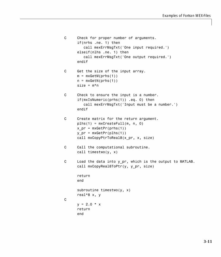
Examples of Fortran MEX-Files
3-11
C Check for proper number of arguments. if(nrhs .ne. 1) then call mexErrMsgTxt('One input required.') elseif(nlhs .ne. 1) then call mexErrMsgTxt('One output required.') endif
C Get the size of the input array. m = mxGetM(prhs(1)) n = mxGetN(prhs(1)) size = m*n
C Check to ensure the input is a number. if(mxIsNumeric(prhs(1)) .eq. 0) then call mexErrMsgTxt('Input must be a number.') endif
C Create matrix for the return argument. plhs(1) = mxCreateFull(m, n, 0) x_pr = mxGetPr(prhs(1)) y_pr = mxGetPr(plhs(1)) call mxCopyPtrToReal8(x_pr, x, size)
C Call the computational subroutine. call timestwo(y, x)
C Load the data into y_pr, which is the output to MATLAB. call mxCopyReal8ToPtr(y, y_pr, size)
return end
subroutine timestwo(y, x) real*8 x, yC y = 2.0 * x return end
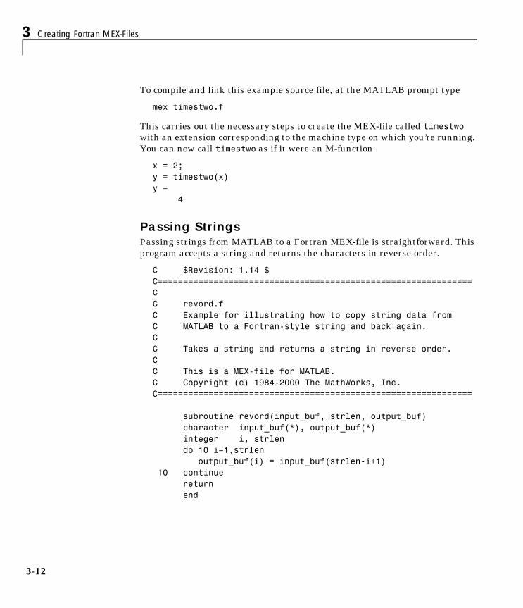
3 Creating Fortran MEX-Files
3-12
To compile and link this example source file, at the MATLAB prompt type
mex timestwo.f
This carries out the necessary steps to create the MEX-file called timestwo with an extension corresponding to the machine type on which you’re running. You can now call timestwo as if it were an M-function.
x = 2;y = timestwo(x)y = 4
Passing StringsPassing strings from MATLAB to a Fortran MEX-file is straightforward. This program accepts a string and returns the characters in reverse order.
C $Revision: 1.14 $C==============================================================C C revord.fC Example for illustrating how to copy string data from C MATLAB to a Fortran-style string and back again. CC Takes a string and returns a string in reverse order. CC This is a MEX-file for MATLAB.C Copyright (c) 1984-2000 The MathWorks, Inc.C==============================================================
subroutine revord(input_buf, strlen, output_buf) character input_buf(*), output_buf(*) integer i, strlen do 10 i=1,strlen output_buf(i) = input_buf(strlen-i+1) 10 continue return end
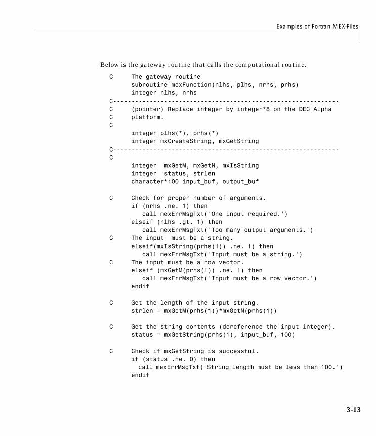
Examples of Fortran MEX-Files
3-13
Below is the gateway routine that calls the computational routine.
C The gateway routine subroutine mexFunction(nlhs, plhs, nrhs, prhs) integer nlhs, nrhsC--------------------------------------------------------------C (pointer) Replace integer by integer*8 on the DEC Alpha C platform.C integer plhs(*), prhs(*) integer mxCreateString, mxGetString C--------------------------------------------------------------C integer mxGetM, mxGetN, mxIsString integer status, strlen character*100 input_buf, output_buf
C Check for proper number of arguments. if (nrhs .ne. 1) then call mexErrMsgTxt('One input required.') elseif (nlhs .gt. 1) then call mexErrMsgTxt('Too many output arguments.')C The input must be a string. elseif(mxIsString(prhs(1)) .ne. 1) then call mexErrMsgTxt('Input must be a string.')C The input must be a row vector. elseif (mxGetM(prhs(1)) .ne. 1) then call mexErrMsgTxt('Input must be a row vector.') endif C Get the length of the input string. strlen = mxGetM(prhs(1))*mxGetN(prhs(1))
C Get the string contents (dereference the input integer). status = mxGetString(prhs(1), input_buf, 100)
C Check if mxGetString is successful. if (status .ne. 0) then call mexErrMsgTxt('String length must be less than 100.') endif
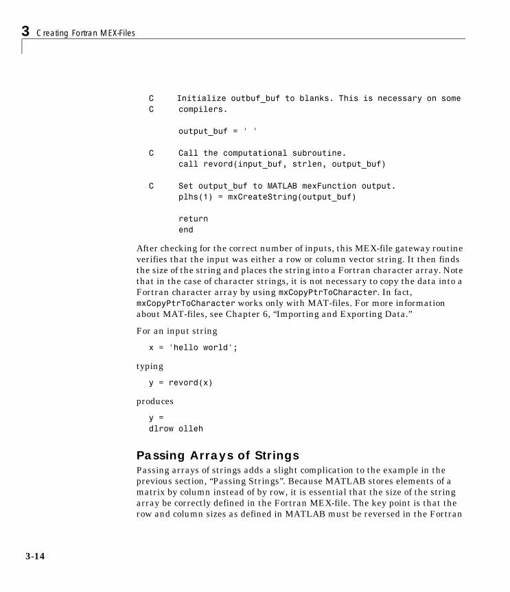
3 Creating Fortran MEX-Files
3-14
C Initialize outbuf_buf to blanks. This is necessary on some C compilers.
output_buf = ' '
C Call the computational subroutine. call revord(input_buf, strlen, output_buf) C Set output_buf to MATLAB mexFunction output. plhs(1) = mxCreateString(output_buf)
return end
After checking for the correct number of inputs, this MEX-file gateway routine verifies that the input was either a row or column vector string. It then finds the size of the string and places the string into a Fortran character array. Note that in the case of character strings, it is not necessary to copy the data into a Fortran character array by using mxCopyPtrToCharacter. In fact, mxCopyPtrToCharacter works only with MAT-files. For more information about MAT-files, see Chapter 6, “Importing and Exporting Data.”
For an input string
x = 'hello world';
typing
y = revord(x)
produces
y =dlrow olleh
Passing Arrays of StringsPassing arrays of strings adds a slight complication to the example in the previous section, “Passing Strings”. Because MATLAB stores elements of a matrix by column instead of by row, it is essential that the size of the string array be correctly defined in the Fortran MEX-file. The key point is that the row and column sizes as defined in MATLAB must be reversed in the Fortran
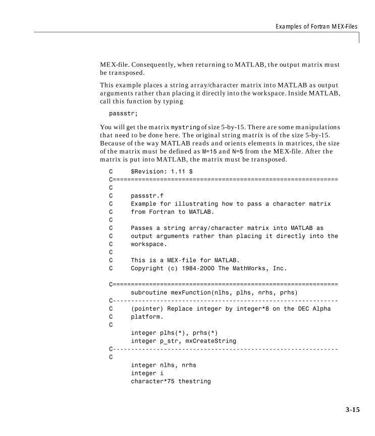
Examples of Fortran MEX-Files
3-15
MEX-file. Consequently, when returning to MATLAB, the output matrix must be transposed.
This example places a string array/character matrix into MATLAB as output arguments rather than placing it directly into the workspace. Inside MATLAB, call this function by typing
passstr;
You will get the matrix mystring of size 5-by-15. There are some manipulations that need to be done here. The original string matrix is of the size 5-by-15. Because of the way MATLAB reads and orients elements in matrices, the size of the matrix must be defined as M=15 and N=5 from the MEX-file. After the matrix is put into MATLAB, the matrix must be transposed.
C $Revision: 1.11 $C==============================================================C C passstr.fC Example for illustrating how to pass a character matrix C from Fortran to MATLAB.C C Passes a string array/character matrix into MATLAB as C output arguments rather than placing it directly into theC workspace.C C This is a MEX-file for MATLAB.C Copyright (c) 1984-2000 The MathWorks, Inc.
C============================================================== subroutine mexFunction(nlhs, plhs, nrhs, prhs)C--------------------------------------------------------------C (pointer) Replace integer by integer*8 on the DEC Alpha C platform.C integer plhs(*), prhs(*) integer p_str, mxCreateStringC--------------------------------------------------------------C integer nlhs, nrhs integer i character*75 thestring
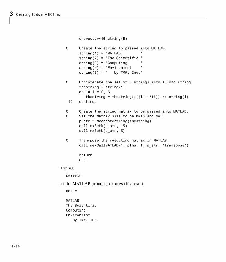
3 Creating Fortran MEX-Files
3-16
character*15 string(5)
C Create the string to passed into MATLAB. string(1) = 'MATLAB ' string(2) = 'The Scientific ' string(3) = 'Computing ' string(4) = 'Environment ' string(5) = ' by TMW, Inc.' C Concatenate the set of 5 strings into a long string. thestring = string(1) do 10 i = 2, 6 thestring = thestring(:((i-1)*15)) // string(i) 10 continue C Create the string matrix to be passed into MATLAB. C Set the matrix size to be M=15 and N=5. p_str = mxcreatestring(thestring) call mxSetM(p_str, 15) call mxSetN(p_str, 5) C Transpose the resulting matrix in MATLAB. call mexCallMATLAB(1, plhs, 1, p_str, 'transpose')
return end
Typing
passstr
at the MATLAB prompt produces this result
ans =
MATLAB The Scientific Computing Environment by TMW, Inc.
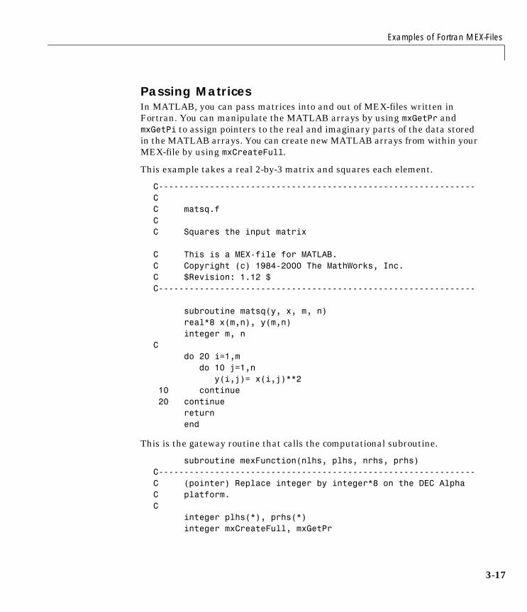
Examples of Fortran MEX-Files
3-17
Passing MatricesIn MATLAB, you can pass matrices into and out of MEX-files written in Fortran. You can manipulate the MATLAB arrays by using mxGetPr and mxGetPi to assign pointers to the real and imaginary parts of the data stored in the MATLAB arrays. You can create new MATLAB arrays from within your MEX-file by using mxCreateFull.
This example takes a real 2-by-3 matrix and squares each element.
C--------------------------------------------------------------C C matsq.fCC Squares the input matrix C This is a MEX-file for MATLAB.C Copyright (c) 1984-2000 The MathWorks, Inc.C $Revision: 1.12 $C--------------------------------------------------------------
subroutine matsq(y, x, m, n) real*8 x(m,n), y(m,n) integer m, nC do 20 i=1,m do 10 j=1,n y(i,j)= x(i,j)**2 10 continue 20 continue return end
This is the gateway routine that calls the computational subroutine.
subroutine mexFunction(nlhs, plhs, nrhs, prhs)C--------------------------------------------------------------C (pointer) Replace integer by integer*8 on the DEC Alpha C platform.C integer plhs(*), prhs(*) integer mxCreateFull, mxGetPr
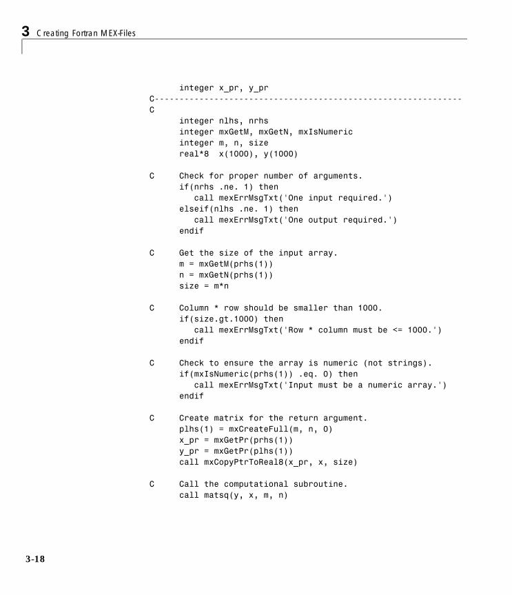
3 Creating Fortran MEX-Files
3-18
integer x_pr, y_prC--------------------------------------------------------------C integer nlhs, nrhs integer mxGetM, mxGetN, mxIsNumeric integer m, n, size real*8 x(1000), y(1000)
C Check for proper number of arguments. if(nrhs .ne. 1) then call mexErrMsgTxt('One input required.') elseif(nlhs .ne. 1) then call mexErrMsgTxt('One output required.') endif
C Get the size of the input array. m = mxGetM(prhs(1)) n = mxGetN(prhs(1)) size = m*n
C Column * row should be smaller than 1000. if(size.gt.1000) then call mexErrMsgTxt('Row * column must be <= 1000.') endif C Check to ensure the array is numeric (not strings). if(mxIsNumeric(prhs(1)) .eq. 0) then call mexErrMsgTxt('Input must be a numeric array.') endif
C Create matrix for the return argument. plhs(1) = mxCreateFull(m, n, 0) x_pr = mxGetPr(prhs(1)) y_pr = mxGetPr(plhs(1)) call mxCopyPtrToReal8(x_pr, x, size)
C Call the computational subroutine. call matsq(y, x, m, n)
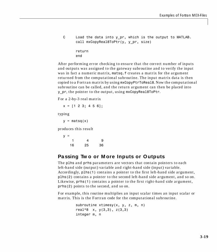
Examples of Fortran MEX-Files
3-19
C Load the data into y_pr, which is the output to MATLAB. call mxCopyReal8ToPtr(y, y_pr, size)
return end
After performing error checking to ensure that the correct number of inputs and outputs was assigned to the gateway subroutine and to verify the input was in fact a numeric matrix, matsq.f creates a matrix for the argument returned from the computational subroutine. The input matrix data is then copied to a Fortran matrix by using mxCopyPtrToReal8. Now the computational subroutine can be called, and the return argument can then be placed into y_pr, the pointer to the output, using mxCopyReal8ToPtr.
For a 2-by-3 real matrix
x = [1 2 3; 4 5 6];
typing
y = matsq(x)
produces this result
y =1 4 9
16 25 36
Passing Two or More Inputs or OutputsThe plhs and prhs parameters are vectors that contain pointers to each left-hand side (output) variable and right-hand side (input) variable. Accordingly, plhs(1) contains a pointer to the first left-hand side argument, plhs(2) contains a pointer to the second left-hand side argument, and so on. Likewise, prhs(1) contains a pointer to the first right-hand side argument, prhs(2) points to the second, and so on.
For example, this routine multiplies an input scalar times an input scalar or matrix. This is the Fortran code for the computational subroutine.
subroutine xtimesy(x, y, z, m, n) real*8 x, y(3,3), z(3,3) integer m, n
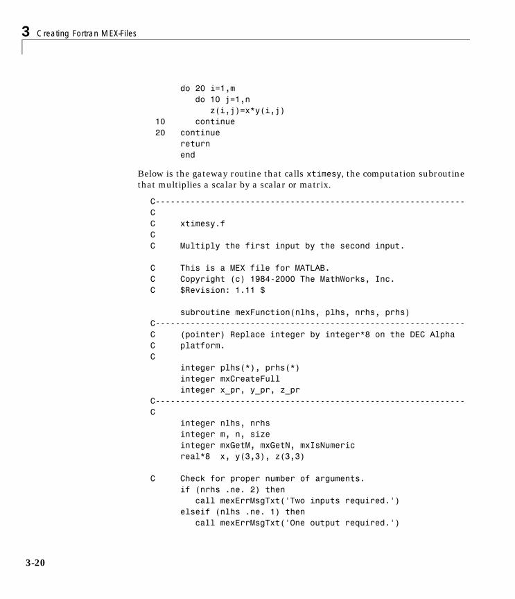
3 Creating Fortran MEX-Files
3-20
do 20 i=1,m do 10 j=1,n z(i,j)=x*y(i,j) 10 continue 20 continue return end
Below is the gateway routine that calls xtimesy, the computation subroutine that multiplies a scalar by a scalar or matrix.
C--------------------------------------------------------------CC xtimesy.fCC Multiply the first input by the second input. C This is a MEX file for MATLAB.C Copyright (c) 1984-2000 The MathWorks, Inc.C $Revision: 1.11 $ subroutine mexFunction(nlhs, plhs, nrhs, prhs)C--------------------------------------------------------------C (pointer) Replace integer by integer*8 on the DEC Alpha C platform.C integer plhs(*), prhs(*) integer mxCreateFull integer x_pr, y_pr, z_prC--------------------------------------------------------------C integer nlhs, nrhs integer m, n, size integer mxGetM, mxGetN, mxIsNumeric real*8 x, y(3,3), z(3,3)
C Check for proper number of arguments. if (nrhs .ne. 2) then call mexErrMsgTxt('Two inputs required.') elseif (nlhs .ne. 1) then call mexErrMsgTxt('One output required.')
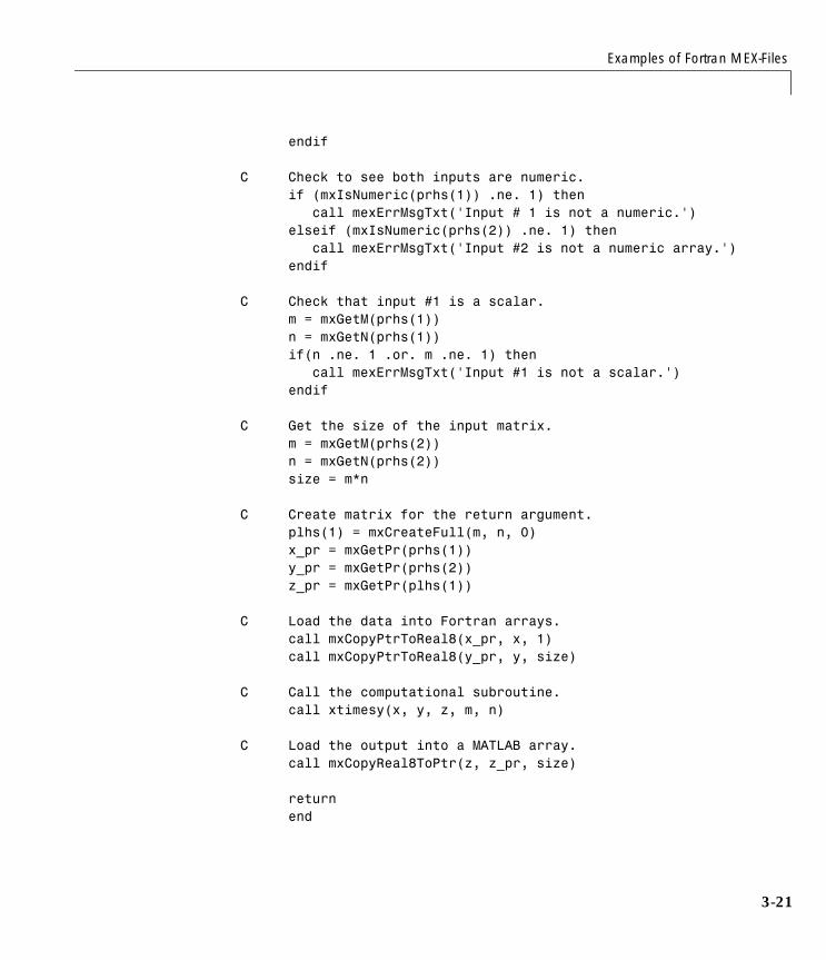
Examples of Fortran MEX-Files
3-21
endif
C Check to see both inputs are numeric. if (mxIsNumeric(prhs(1)) .ne. 1) then call mexErrMsgTxt('Input # 1 is not a numeric.') elseif (mxIsNumeric(prhs(2)) .ne. 1) then call mexErrMsgTxt('Input #2 is not a numeric array.') endif C Check that input #1 is a scalar. m = mxGetM(prhs(1)) n = mxGetN(prhs(1)) if(n .ne. 1 .or. m .ne. 1) then call mexErrMsgTxt('Input #1 is not a scalar.') endif
C Get the size of the input matrix. m = mxGetM(prhs(2)) n = mxGetN(prhs(2)) size = m*n
C Create matrix for the return argument. plhs(1) = mxCreateFull(m, n, 0) x_pr = mxGetPr(prhs(1)) y_pr = mxGetPr(prhs(2)) z_pr = mxGetPr(plhs(1))
C Load the data into Fortran arrays. call mxCopyPtrToReal8(x_pr, x, 1) call mxCopyPtrToReal8(y_pr, y, size)
C Call the computational subroutine. call xtimesy(x, y, z, m, n)
C Load the output into a MATLAB array. call mxCopyReal8ToPtr(z, z_pr, size)
return end
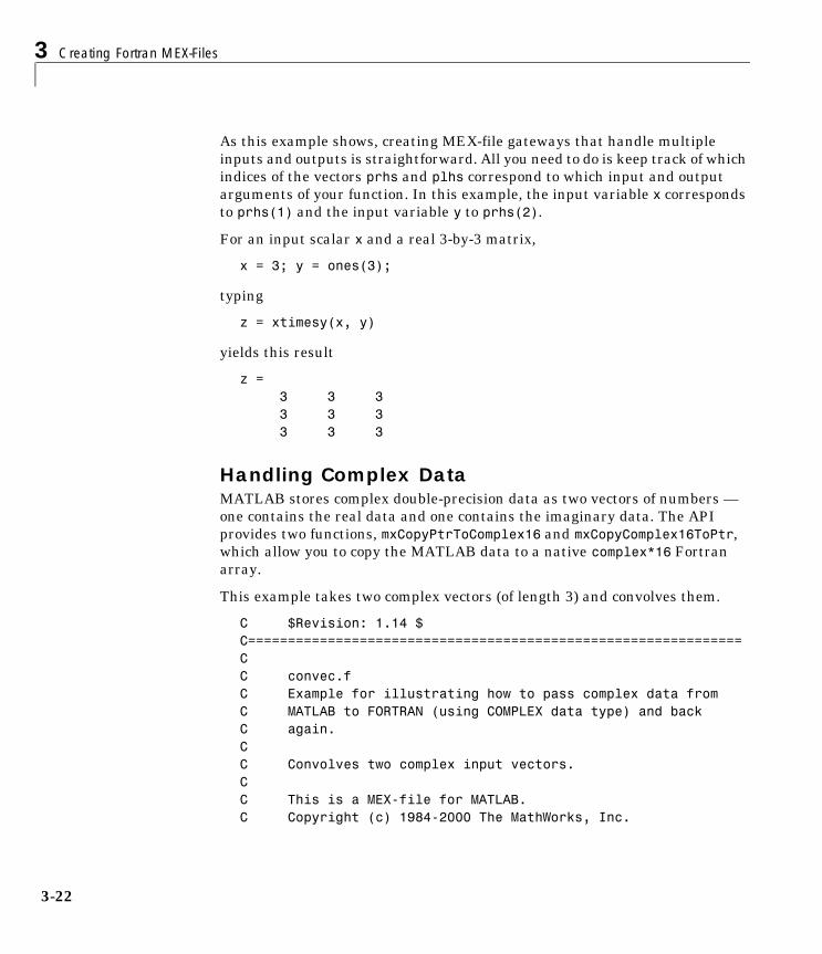
3 Creating Fortran MEX-Files
3-22
As this example shows, creating MEX-file gateways that handle multiple inputs and outputs is straightforward. All you need to do is keep track of which indices of the vectors prhs and plhs correspond to which input and output arguments of your function. In this example, the input variable x corresponds to prhs(1) and the input variable y to prhs(2).
For an input scalar x and a real 3-by-3 matrix,
x = 3; y = ones(3);
typing
z = xtimesy(x, y)
yields this result
z = 3 3 3 3 3 3 3 3 3
Handling Complex DataMATLAB stores complex double-precision data as two vectors of numbers — one contains the real data and one contains the imaginary data. The API provides two functions, mxCopyPtrToComplex16 and mxCopyComplex16ToPtr, which allow you to copy the MATLAB data to a native complex*16 Fortran array.
This example takes two complex vectors (of length 3) and convolves them.
C $Revision: 1.14 $C==============================================================CC convec.fC Example for illustrating how to pass complex data from C MATLAB to FORTRAN (using COMPLEX data type) and back C again.C C Convolves two complex input vectors.C C This is a MEX-file for MATLAB.C Copyright (c) 1984-2000 The MathWorks, Inc.
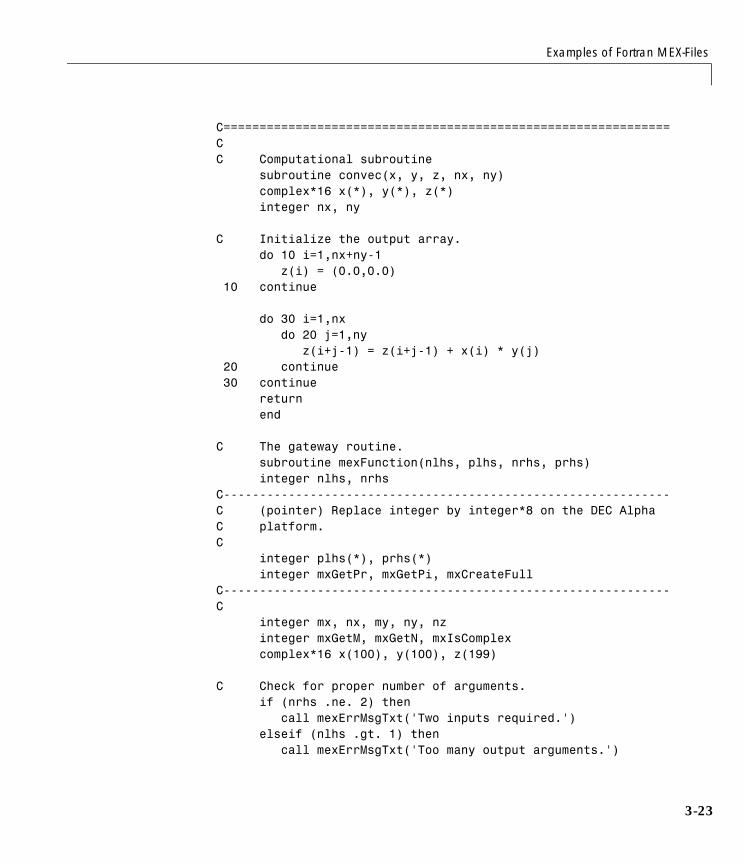
Examples of Fortran MEX-Files
3-23
C==============================================================CC Computational subroutine subroutine convec(x, y, z, nx, ny) complex*16 x(*), y(*), z(*) integer nx, ny
C Initialize the output array. do 10 i=1,nx+ny-1 z(i) = (0.0,0.0) 10 continue
do 30 i=1,nx do 20 j=1,ny z(i+j-1) = z(i+j-1) + x(i) * y(j) 20 continue 30 continue return end
C The gateway routine. subroutine mexFunction(nlhs, plhs, nrhs, prhs) integer nlhs, nrhsC--------------------------------------------------------------C (pointer) Replace integer by integer*8 on the DEC Alpha C platform.C integer plhs(*), prhs(*) integer mxGetPr, mxGetPi, mxCreateFullC--------------------------------------------------------------C integer mx, nx, my, ny, nz integer mxGetM, mxGetN, mxIsComplex complex*16 x(100), y(100), z(199)
C Check for proper number of arguments. if (nrhs .ne. 2) then call mexErrMsgTxt('Two inputs required.') elseif (nlhs .gt. 1) then call mexErrMsgTxt('Too many output arguments.')
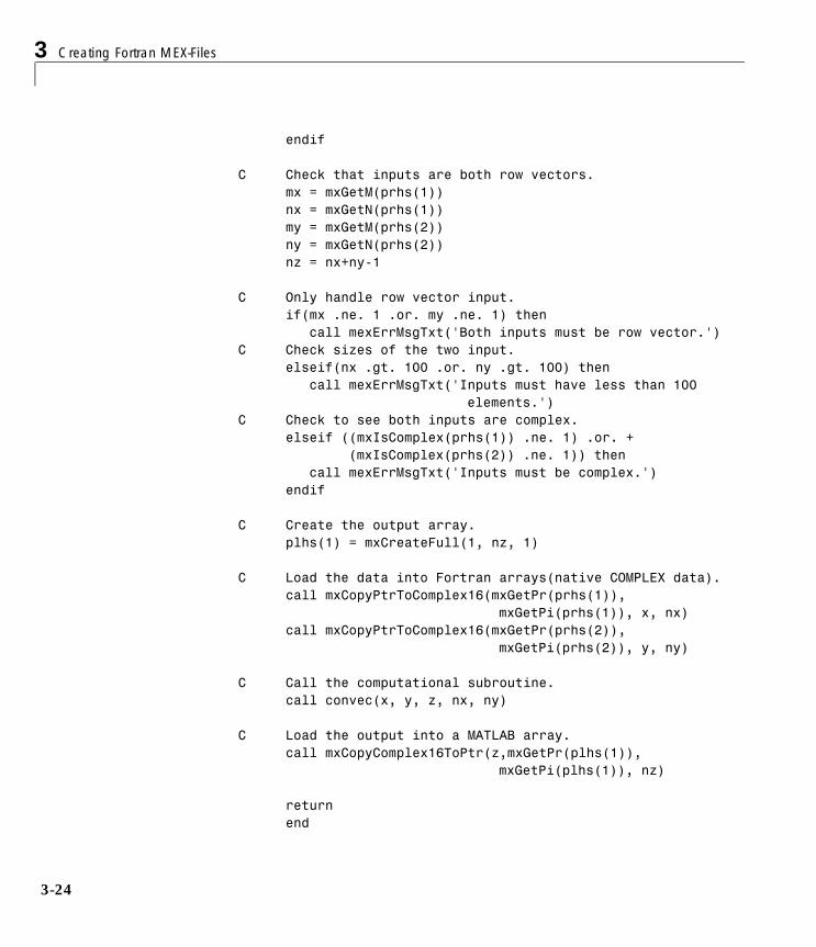
3 Creating Fortran MEX-Files
3-24
endif
C Check that inputs are both row vectors. mx = mxGetM(prhs(1)) nx = mxGetN(prhs(1)) my = mxGetM(prhs(2)) ny = mxGetN(prhs(2)) nz = nx+ny-1
C Only handle row vector input. if(mx .ne. 1 .or. my .ne. 1) then call mexErrMsgTxt('Both inputs must be row vector.')C Check sizes of the two input. elseif(nx .gt. 100 .or. ny .gt. 100) then call mexErrMsgTxt('Inputs must have less than 100 elements.')C Check to see both inputs are complex. elseif ((mxIsComplex(prhs(1)) .ne. 1) .or. + (mxIsComplex(prhs(2)) .ne. 1)) then call mexErrMsgTxt('Inputs must be complex.') endif
C Create the output array. plhs(1) = mxCreateFull(1, nz, 1)
C Load the data into Fortran arrays(native COMPLEX data). call mxCopyPtrToComplex16(mxGetPr(prhs(1)), mxGetPi(prhs(1)), x, nx) call mxCopyPtrToComplex16(mxGetPr(prhs(2)), mxGetPi(prhs(2)), y, ny)
C Call the computational subroutine. call convec(x, y, z, nx, ny)
C Load the output into a MATLAB array. call mxCopyComplex16ToPtr(z,mxGetPr(plhs(1)), mxGetPi(plhs(1)), nz)
return end
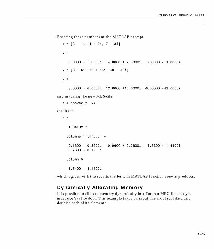
Examples of Fortran MEX-Files
3-25
Entering these numbers at the MATLAB prompt
x = [3 - 1i, 4 + 2i, 7 - 3i]
x =
3.0000 - 1.0000i 4.0000 + 2.0000i 7.0000 - 3.0000i
y = [8 - 6i, 12 + 16i, 40 - 42i]
y =
8.0000 - 6.0000i 12.0000 +16.0000i 40.0000 -42.0000i
and invoking the new MEX-file
z = convec(x, y)
results in
z =
1.0e+02 *
Columns 1 through 4
0.1800 - 0.2600i 0.9600 + 0.2800i 1.3200 - 1.4400i 3.7600 - 0.1200i
Column 5
1.5400 - 4.1400i
which agrees with the results the built-in MATLAB function conv.m produces.
Dynamically Allocating MemoryIt is possible to allocate memory dynamically in a Fortran MEX-file, but you must use %val to do it. This example takes an input matrix of real data and doubles each of its elements.
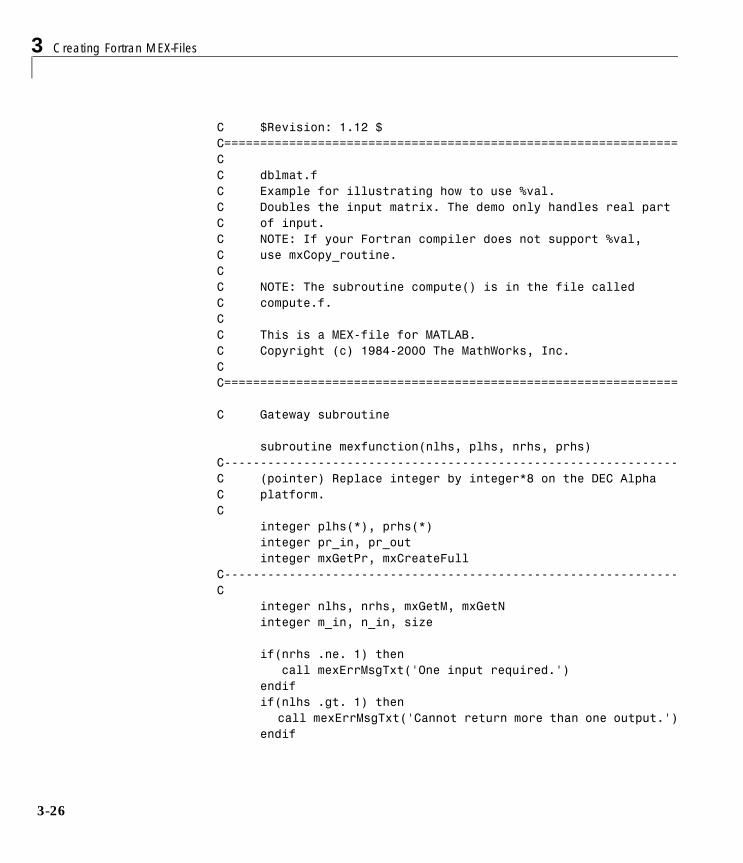
3 Creating Fortran MEX-Files
3-26
C $Revision: 1.12 $C===============================================================C C dblmat.fC Example for illustrating how to use %val.C Doubles the input matrix. The demo only handles real partC of input.C NOTE: If your Fortran compiler does not support %val, C use mxCopy_routine.CC NOTE: The subroutine compute() is in the file calledC compute.f. CC This is a MEX-file for MATLAB.C Copyright (c) 1984-2000 The MathWorks, Inc.C C===============================================================
C Gateway subroutine
subroutine mexfunction(nlhs, plhs, nrhs, prhs)C---------------------------------------------------------------C (pointer) Replace integer by integer*8 on the DEC Alpha C platform.C integer plhs(*), prhs(*) integer pr_in, pr_out integer mxGetPr, mxCreateFullC---------------------------------------------------------------C integer nlhs, nrhs, mxGetM, mxGetN integer m_in, n_in, size
if(nrhs .ne. 1) then call mexErrMsgTxt('One input required.') endif if(nlhs .gt. 1) then call mexErrMsgTxt('Cannot return more than one output.') endif
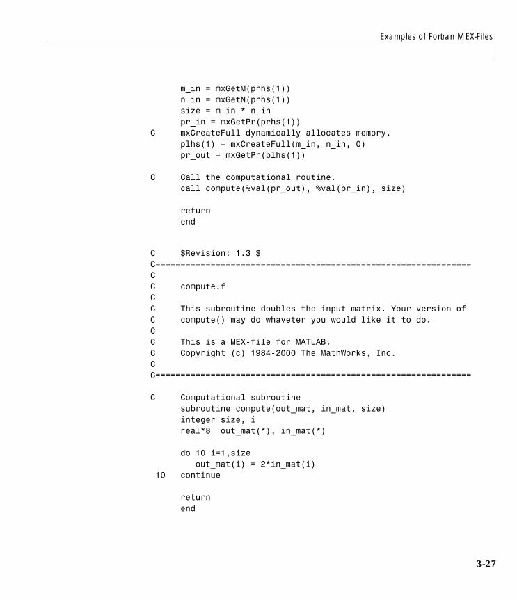
Examples of Fortran MEX-Files
3-27
m_in = mxGetM(prhs(1)) n_in = mxGetN(prhs(1)) size = m_in * n_in pr_in = mxGetPr(prhs(1))C mxCreateFull dynamically allocates memory. plhs(1) = mxCreateFull(m_in, n_in, 0) pr_out = mxGetPr(plhs(1))
C Call the computational routine. call compute(%val(pr_out), %val(pr_in), size)
return end
C $Revision: 1.3 $C===============================================================C C compute.fCC This subroutine doubles the input matrix. Your version of C compute() may do whaveter you would like it to do.CC This is a MEX-file for MATLAB.C Copyright (c) 1984-2000 The MathWorks, Inc. C C===============================================================
C Computational subroutine subroutine compute(out_mat, in_mat, size) integer size, i real*8 out_mat(*), in_mat(*)
do 10 i=1,size out_mat(i) = 2*in_mat(i) 10 continue
return end
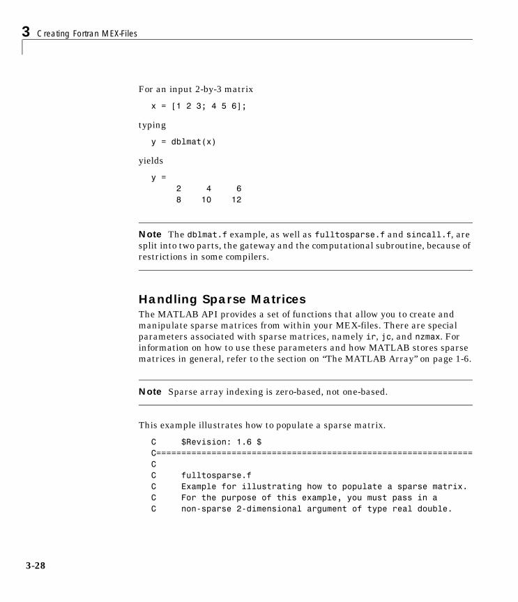
3 Creating Fortran MEX-Files
3-28
For an input 2-by-3 matrix
x = [1 2 3; 4 5 6];
typing
y = dblmat(x)
yields
y = 2 4 6 8 10 12
Note The dblmat.f example, as well as fulltosparse.f and sincall.f, are split into two parts, the gateway and the computational subroutine, because of restrictions in some compilers.
Handling Sparse Matrices The MATLAB API provides a set of functions that allow you to create and manipulate sparse matrices from within your MEX-files. There are special parameters associated with sparse matrices, namely ir, jc, and nzmax. For information on how to use these parameters and how MATLAB stores sparse matrices in general, refer to the section on “The MATLAB Array” on page 1-6.
Note Sparse array indexing is zero-based, not one-based.
This example illustrates how to populate a sparse matrix.
C $Revision: 1.6 $C===============================================================CC fulltosparse.fC Example for illustrating how to populate a sparse matrix.C For the purpose of this example, you must pass in aC non-sparse 2-dimensional argument of type real double.
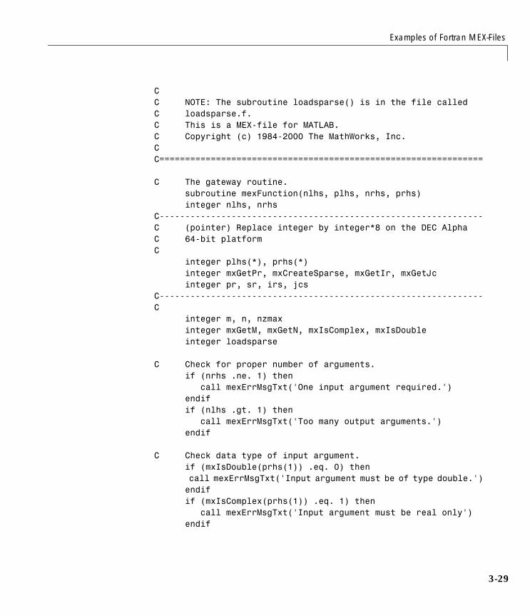
Examples of Fortran MEX-Files
3-29
CC NOTE: The subroutine loadsparse() is in the file called C loadsparse.f. C This is a MEX-file for MATLAB.C Copyright (c) 1984-2000 The MathWorks, Inc. C C===============================================================
C The gateway routine. subroutine mexFunction(nlhs, plhs, nrhs, prhs) integer nlhs, nrhsC---------------------------------------------------------------C (pointer) Replace integer by integer*8 on the DEC AlphaC 64-bit platformC integer plhs(*), prhs(*) integer mxGetPr, mxCreateSparse, mxGetIr, mxGetJc integer pr, sr, irs, jcsC---------------------------------------------------------------C integer m, n, nzmax integer mxGetM, mxGetN, mxIsComplex, mxIsDouble integer loadsparse
C Check for proper number of arguments. if (nrhs .ne. 1) then call mexErrMsgTxt('One input argument required.') endif if (nlhs .gt. 1) then call mexErrMsgTxt('Too many output arguments.') endif
C Check data type of input argument. if (mxIsDouble(prhs(1)) .eq. 0) then call mexErrMsgTxt('Input argument must be of type double.') endif if (mxIsComplex(prhs(1)) .eq. 1) then call mexErrMsgTxt('Input argument must be real only') endif
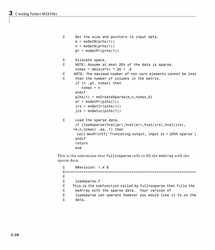
3 Creating Fortran MEX-Files
3-30
C Get the size and pointers to input data. m = mxGetM(prhs(1)) n = mxGetN(prhs(1)) pr = mxGetPr(prhs(1))
C Allocate space.C NOTE: Assume at most 20% of the data is sparse. nzmax = dble(m*n) *.20 + .5C NOTE: The maximum number of non-zero elements cannot be lessC than the number of columns in the matrix. if (n .gt. nzmax) then nzmax = n endif plhs(1) = mxCreateSparse(m,n,nzmax,0) sr = mxGetPr(plhs(1)) irs = mxGetIr(plhs(1)) jcs = mxGetJc(plhs(1))
C Load the sparse data. if (loadsparse(%val(pr),%val(sr),%val(irs),%val(jcs), +m,n,nzmax) .eq. 1) then call mexPrintf('Truncating output, input is > 20%% sparse') endif return end
This is the subroutine that fulltosparse calls to fill the mxArray with the sparse data.
C $Revision: 1.4 $C===============================================================C C loadsparse.fC This is the subfunction called by fulltosparse that fills the C mxArray with the sparse data. Your version ofC loadsparse can operate however you would like it to on theC data.
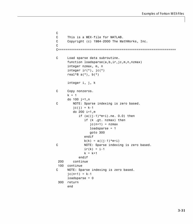
Examples of Fortran MEX-Files
3-31
CC This is a MEX-file for MATLAB.C Copyright (c) 1984-2000 The MathWorks, Inc. C C===============================================================
C Load sparse data subroutine. function loadsparse(a,b,ir,jc,m,n,nzmax) integer nzmax, m, n integer ir(*), jc(*) real*8 a(*), b(*)
integer i, j, k
C Copy nonzeros. k = 1 do 100 j=1,nC NOTE: Sparse indexing is zero based. jc(j) = k-1 do 200 i=1,m if (a((j-1)*m+i).ne. 0.0) then if (k .gt. nzmax) then jc(n+1) = nzmax loadsparse = 1 goto 300 endif b(k) = a((j-1)*m+i)C NOTE: Sparse indexing is zero based. ir(k) = i-1 k = k+1 endif 200 continue 100 continueC NOTE: Sparse indexing is zero based. jc(n+1) = k-1 loadsparse = 0 300 return end
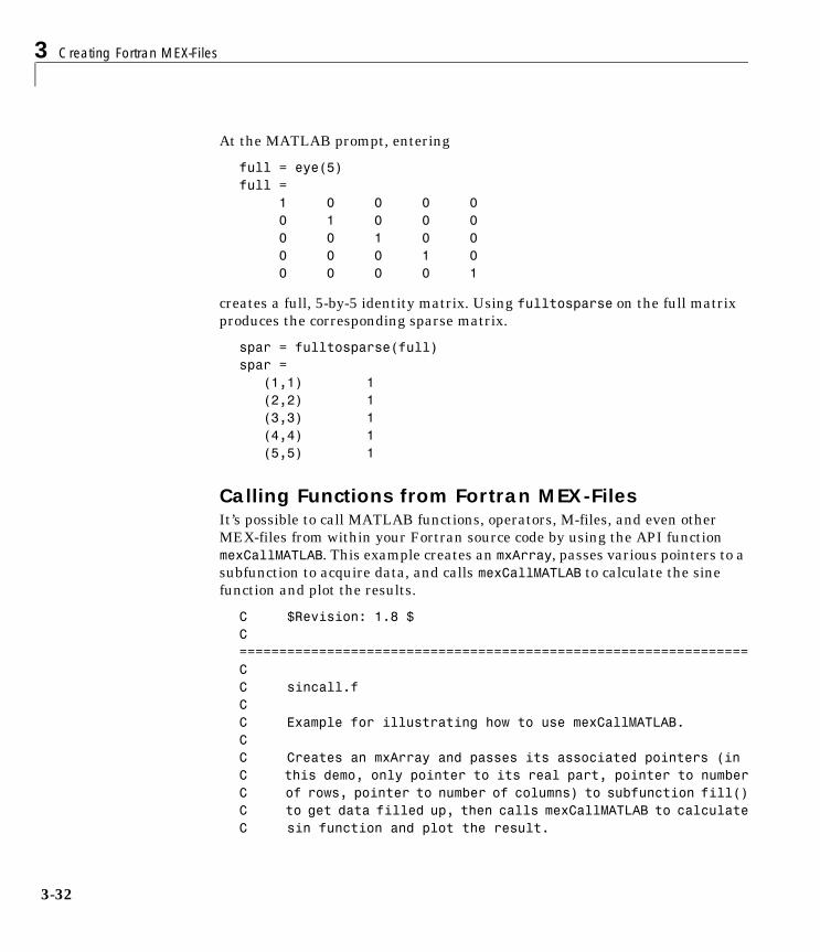
3 Creating Fortran MEX-Files
3-32
At the MATLAB prompt, entering
full = eye(5)full = 1 0 0 0 0 0 1 0 0 0 0 0 1 0 0 0 0 0 1 0 0 0 0 0 1
creates a full, 5-by-5 identity matrix. Using fulltosparse on the full matrix produces the corresponding sparse matrix.
spar = fulltosparse(full)spar = (1,1) 1 (2,2) 1 (3,3) 1 (4,4) 1 (5,5) 1
Calling Functions from Fortran MEX-FilesIt’s possible to call MATLAB functions, operators, M-files, and even other MEX-files from within your Fortran source code by using the API function mexCallMATLAB. This example creates an mxArray, passes various pointers to a subfunction to acquire data, and calls mexCallMATLAB to calculate the sine function and plot the results.
C $Revision: 1.8 $C ================================================================C C sincall.fCC Example for illustrating how to use mexCallMATLAB.C C Creates an mxArray and passes its associated pointers (inC this demo, only pointer to its real part, pointer to numberC of rows, pointer to number of columns) to subfunction fill()C to get data filled up, then calls mexCallMATLAB to calculateC sin function and plot the result.
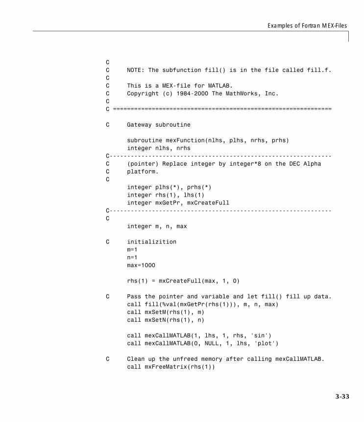
Examples of Fortran MEX-Files
3-33
CC NOTE: The subfunction fill() is in the file called fill.f.CC This is a MEX-file for MATLAB.C Copyright (c) 1984-2000 The MathWorks, Inc.C C ==============================================================
C Gateway subroutine
subroutine mexFunction(nlhs, plhs, nrhs, prhs) integer nlhs, nrhsC---------------------------------------------------------------C (pointer) Replace integer by integer*8 on the DEC Alpha C platform.C integer plhs(*), prhs(*) integer rhs(1), lhs(1) integer mxGetPr, mxCreateFullC---------------------------------------------------------------C integer m, n, max C initializition m=1 n=1 max=1000
rhs(1) = mxCreateFull(max, 1, 0) C Pass the pointer and variable and let fill() fill up data. call fill(%val(mxGetPr(rhs(1))), m, n, max) call mxSetM(rhs(1), m) call mxSetN(rhs(1), n)
call mexCallMATLAB(1, lhs, 1, rhs, 'sin') call mexCallMATLAB(0, NULL, 1, lhs, 'plot')
C Clean up the unfreed memory after calling mexCallMATLAB. call mxFreeMatrix(rhs(1))
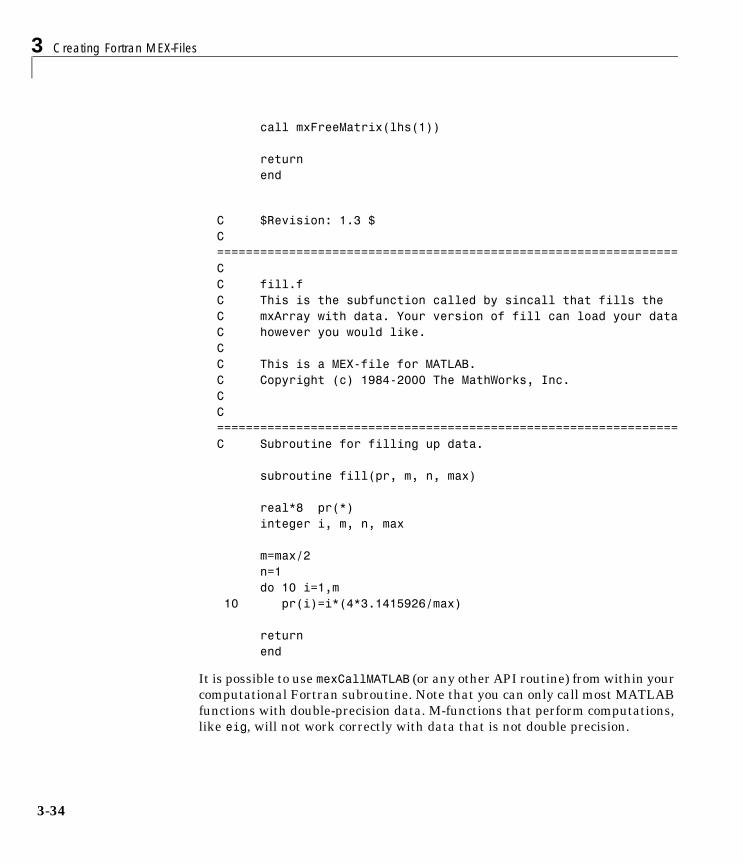
3 Creating Fortran MEX-Files
3-34
call mxFreeMatrix(lhs(1))
return end
C $Revision: 1.3 $C ================================================================C C fill.fC This is the subfunction called by sincall that fills the C mxArray with data. Your version of fill can load your dataC however you would like.CC This is a MEX-file for MATLAB.C Copyright (c) 1984-2000 The MathWorks, Inc. C C ================================================================C Subroutine for filling up data.
subroutine fill(pr, m, n, max) real*8 pr(*) integer i, m, n, max m=max/2 n=1 do 10 i=1,m 10 pr(i)=i*(4*3.1415926/max)
return end
It is possible to use mexCallMATLAB (or any other API routine) from within your computational Fortran subroutine. Note that you can only call most MATLAB functions with double-precision data. M-functions that perform computations, like eig, will not work correctly with data that is not double precision.
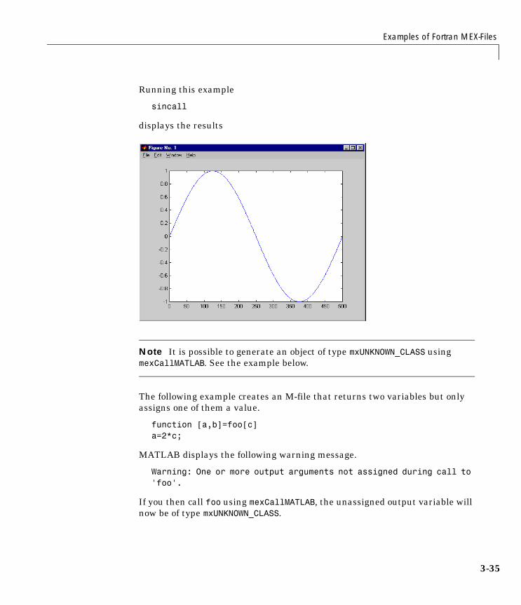
Examples of Fortran MEX-Files
3-35
Running this example
sincall
displays the results
Note It is possible to generate an object of type mxUNKNOWN_CLASS using mexCallMATLAB. See the example below.
The following example creates an M-file that returns two variables but only assigns one of them a value.
function [a,b]=foo[c]a=2*c;
MATLAB displays the following warning message.
Warning: One or more output arguments not assigned during call to 'foo'.
If you then call foo using mexCallMATLAB, the unassigned output variable will now be of type mxUNKNOWN_CLASS.
3 Creating Fortran MEX-Files
3-36
Advanced TopicsThese sections cover advanced features of MEX-files that you can use when your applications require sophisticated MEX-files.
Help FilesBecause the MATLAB interpreter chooses the MEX-file when both an M-file and a MEX-file with the same name are encountered in the same directory, it is possible to use M-files for documenting the behavior of your MEX-files. The MATLAB help command will automatically find and display the appropriate M-file when help is requested and the interpreter will find and execute the corresponding MEX-file when the function is actually invoked.
Linking Multiple FilesYou can combine several source files when building MEX-files. For example,
mex circle.f square.o rectangle.f shapes.o
is a legal command that operates on the .f and .o files to create a MEX-file called circle.ext, where ext is the extension corresponding to the MEX-file type. The name of the resulting MEX-file is taken from the first file in the list.
You may find it useful to use a software development tool like MAKE to manage MEX-file projects involving multiple source files. Simply create a MAKEFILE that contains a rule for producing object files from each of your source files and then invoke mex to combine your object files into a MEX-file. This way you can ensure that your source files are recompiled only when necessary.
Note On UNIX, you must use the -fortran switch to the mex script if you are linking Fortran objects.
Workspace for MEX-File FunctionsUnlike M-file functions, MEX-file functions do not have their own variable workspace. mexEvalString evaluates the string in the caller’s workspace. In addition, you can use the mexGetMatrix and mexPutMatrix routines to get and put variables into the caller’s workspace.
Advanced Topics
3-37
Memory ManagementAs of Version 5.2, MATLAB now implicitly destroys (by calling mxDestroyArray) any arrays created by a MEX-file that are not returned in the left-hand side list (plhs()). Consequently, any misconstructed arrays left over at the end of a MEX-file’s execution have the potential to cause memory errors.
In general, we recommend that MEX-files destroy their own temporary arrays and clean up their own temporary memory. For additional information on memory management techniques, see the sections “Memory Management” on page 2-38 and “Memory Management Compatibility Issues” on page 1-37.
3 Creating Fortran MEX-Files
3-38
Debugging Fortran Language MEX-FilesOn most platforms, it is now possible to debug MEX-files while they are running within MATLAB. Complete source code debugging, including setting breakpoints, examining variables, and stepping through the source code line-by-line, is now available.
Note The section on “Troubleshooting” on page 1-32 provides additional information on isolating problems with MEX-files.
To debug a MEX-file from within MATLAB, you must first compile the MEX-file with the -g option to mex.
mex -g filename.f
Debugging on UNIXYou must start MATLAB from within a debugger. To do this, specify the name of the debugger you want to use with the -D option when starting MATLAB. For example, to use dbx, the UNIX debugger, type
matlab -Ddbx
Once the debugger loads MATLAB into memory, you can start it by issuing a run command. Now, from within MATLAB, enable MEX-file debugging by typing
dbmex on
at the MATLAB prompt. Then run the MEX-file you want to debug as you would ordinarily (either directly or by means of some other function or script). Before executing the MEX-file, you will be returned to the debugger.
You may need to tell the debugger where the MEX-file was loaded or the name of the MEX-file, in which case MATLAB will display the appropriate command for you to use. At this point, you are ready to start debugging. You can list the source code for your MEX-file and set break points in it. It is often convenient to set one at mexFunction so that you stop at the beginning of the gateway routine.
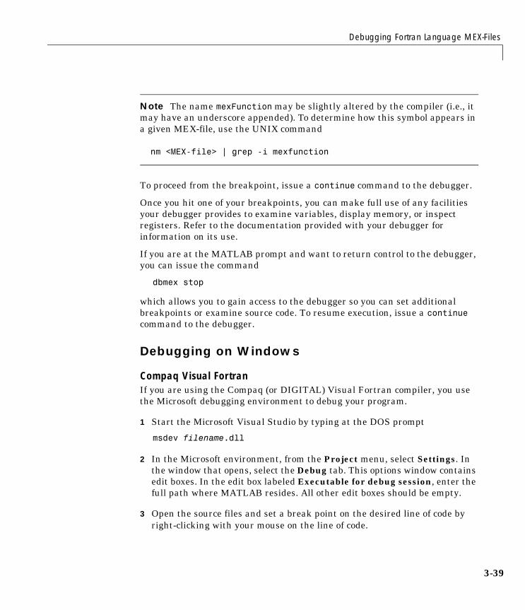
Debugging Fortran Language MEX-Files
3-39
Note The name mexFunction may be slightly altered by the compiler (i.e., it may have an underscore appended). To determine how this symbol appears in a given MEX-file, use the UNIX command
nm <MEX-file> | grep -i mexfunction
To proceed from the breakpoint, issue a continue command to the debugger.
Once you hit one of your breakpoints, you can make full use of any facilities your debugger provides to examine variables, display memory, or inspect registers. Refer to the documentation provided with your debugger for information on its use.
If you are at the MATLAB prompt and want to return control to the debugger, you can issue the command
dbmex stop
which allows you to gain access to the debugger so you can set additional breakpoints or examine source code. To resume execution, issue a continue command to the debugger.
Debugging on Windows
Compaq Visual FortranIf you are using the Compaq (or DIGITAL) Visual Fortran compiler, you use the Microsoft debugging environment to debug your program.
1 Start the Microsoft Visual Studio by typing at the DOS prompt
msdev filename.dll
2 In the Microsoft environment, from the Project menu, select Settings. In the window that opens, select the Debug tab. This options window contains edit boxes. In the edit box labeled Executable for debug session, enter the full path where MATLAB resides. All other edit boxes should be empty.
3 Open the source files and set a break point on the desired line of code by right-clicking with your mouse on the line of code.
3 Creating Fortran MEX-Files
3-40
4 From the Build menu, select Debug, and click Go.
5 You will now be able to run your MEX-file in MATLAB and use the Microsoft debugging environment. For more information on how to debug in the Microsoft environment, see the Microsoft Development Studio documentation.
4Calling MATLAB from C and Fortran Programs
Using the MATLAB Engine . . . . . . . . . . . . . 4-3The Engine Library . . . . . . . . . . . . . . . . . . 4-3GUI-Intensive Applications . . . . . . . . . . . . . . 4-5
Examples of Calling Engine Functions . . . . . . . . 4-6Calling MATLAB From a C Application . . . . . . . . . 4-6Calling MATLAB From a Fortran Application . . . . . . . 4-11Attaching to an Existing MATLAB Session . . . . . . . . 4-15
Compiling and Linking Engine Programs . . . . . . . 4-17Masking Floating-Point Exceptions . . . . . . . . . . . 4-17Compiling and Linking on UNIX . . . . . . . . . . . . 4-18Compiling and Linking on Windows . . . . . . . . . . . 4-19
4 Calling MATLAB from C and Fortran Programs
4-2
The MATLAB engine library is a set of routines that allows you to call MATLAB from your own programs, thereby employing MATLAB as a computation engine. MATLAB engine programs are C or Fortran programs that communicate with a separate MATLAB process via pipes (in UNIX) and through ActiveX on Windows. There is a library of functions provided with MATLAB that allows you to start and end the MATLAB process, send data to and from MATLAB, and send commands to be processed in MATLAB.
The following list summarizes the contents of this chapter:
• “Using the MATLAB Engine”
• “Examples of Calling Engine Functions”
• “Compiling and Linking Engine Programs”
For additional information and support in building your applications, see the section entitled “Additional Information” on page 1-42.
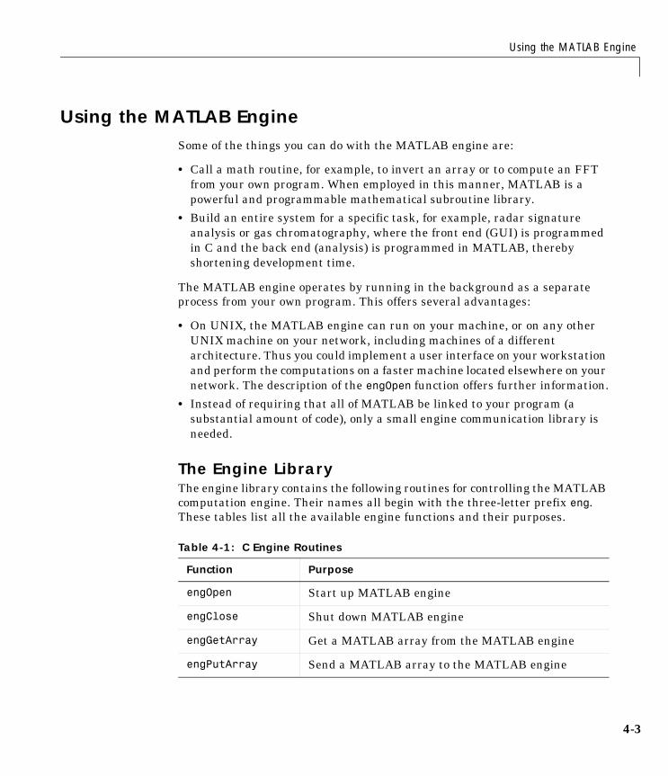
Using the MATLAB Engine
4-3
Using the MATLAB EngineSome of the things you can do with the MATLAB engine are:
• Call a math routine, for example, to invert an array or to compute an FFT from your own program. When employed in this manner, MATLAB is a powerful and programmable mathematical subroutine library.
• Build an entire system for a specific task, for example, radar signature analysis or gas chromatography, where the front end (GUI) is programmed in C and the back end (analysis) is programmed in MATLAB, thereby shortening development time.
The MATLAB engine operates by running in the background as a separate process from your own program. This offers several advantages:
• On UNIX, the MATLAB engine can run on your machine, or on any other UNIX machine on your network, including machines of a different architecture. Thus you could implement a user interface on your workstation and perform the computations on a faster machine located elsewhere on your network. The description of the engOpen function offers further information.
• Instead of requiring that all of MATLAB be linked to your program (a substantial amount of code), only a small engine communication library is needed.
The Engine LibraryThe engine library contains the following routines for controlling the MATLAB computation engine. Their names all begin with the three-letter prefix eng. These tables list all the available engine functions and their purposes.
Table 4-1: C Engine Routines
Function Purpose
engOpen Start up MATLAB engine
engClose Shut down MATLAB engine
engGetArray Get a MATLAB array from the MATLAB engine
engPutArray Send a MATLAB array to the MATLAB engine
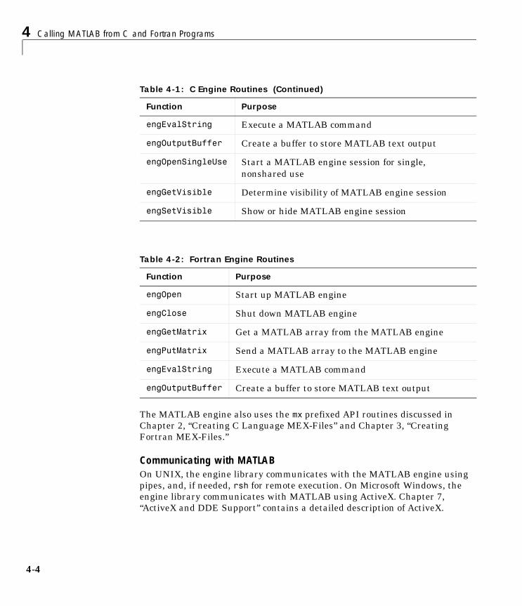
4 Calling MATLAB from C and Fortran Programs
4-4
The MATLAB engine also uses the mx prefixed API routines discussed in Chapter 2, “Creating C Language MEX-Files” and Chapter 3, “Creating Fortran MEX-Files.”
Communicating with MATLABOn UNIX, the engine library communicates with the MATLAB engine using pipes, and, if needed, rsh for remote execution. On Microsoft Windows, the engine library communicates with MATLAB using ActiveX. Chapter 7, “ActiveX and DDE Support” contains a detailed description of ActiveX.
engEvalString Execute a MATLAB command
engOutputBuffer Create a buffer to store MATLAB text output
engOpenSingleUse Start a MATLAB engine session for single, nonshared use
engGetVisible Determine visibility of MATLAB engine session
engSetVisible Show or hide MATLAB engine session
Table 4-2: Fortran Engine Routines
Function Purpose
engOpen Start up MATLAB engine
engClose Shut down MATLAB engine
engGetMatrix Get a MATLAB array from the MATLAB engine
engPutMatrix Send a MATLAB array to the MATLAB engine
engEvalString Execute a MATLAB command
engOutputBuffer Create a buffer to store MATLAB text output
Table 4-1: C Engine Routines (Continued)
Function Purpose
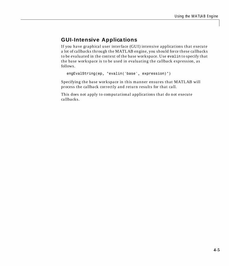
Using the MATLAB Engine
4-5
GUI-Intensive ApplicationsIf you have graphical user interface (GUI) intensive applications that execute a lot of callbacks through the MATLAB engine, you should force these callbacks to be evaluated in the context of the base workspace. Use evalin to specify that the base workspace is to be used in evaluating the callback expression, as follows.
engEvalString(ep, "evalin('base', expression)")
Specifying the base workspace in this manner ensures that MATLAB will process the callback correctly and return results for that call.
This does not apply to computational applications that do not execute callbacks.
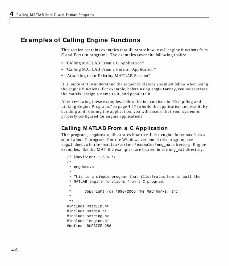
4 Calling MATLAB from C and Fortran Programs
4-6
Examples of Calling Engine FunctionsThis section contains examples that illustrate how to call engine functions from C and Fortran programs. The examples cover the following topics:
• “Calling MATLAB From a C Application”
• “Calling MATLAB From a Fortran Application”
• “Attaching to an Existing MATLAB Session”
It is important to understand the sequence of steps you must follow when using the engine functions. For example, before using engPutArray, you must create the matrix, assign a name to it, and populate it.
After reviewing these examples, follow the instructions in “Compiling and Linking Engine Programs” on page 4-17 to build the application and test it. By building and running the application, you will ensure that your system is properly configured for engine applications.
Calling MATLAB From a C ApplicationThis program, engdemo.c, illustrates how to call the engine functions from a stand-alone C program. For the Windows version of this program, see engwindemo.c in the <matlab>\extern\examples\eng_mat directory. Engine examples, like the MAT-file examples, are located in the eng_mat directory.
/* $Revision: 1.6 $ *//* * engdemo.c * * This is a simple program that illustrates how to call the * MATLAB engine functions from a C program. * * Copyright (c) 1996-2000 The MathWorks, Inc. * */#include <stdlib.h>#include <stdio.h>#include <string.h>#include "engine.h"#define BUFSIZE 256
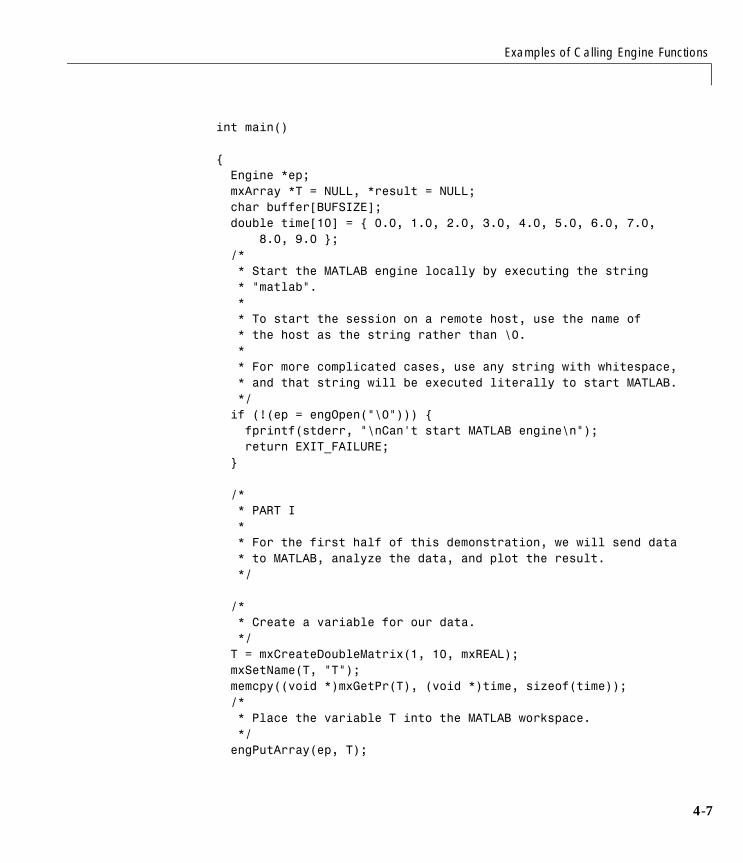
Examples of Calling Engine Functions
4-7
int main()
{ Engine *ep; mxArray *T = NULL, *result = NULL; char buffer[BUFSIZE]; double time[10] = { 0.0, 1.0, 2.0, 3.0, 4.0, 5.0, 6.0, 7.0, 8.0, 9.0 }; /* * Start the MATLAB engine locally by executing the string * "matlab". * * To start the session on a remote host, use the name of * the host as the string rather than \0. * * For more complicated cases, use any string with whitespace, * and that string will be executed literally to start MATLAB. */ if (!(ep = engOpen("\0"))) { fprintf(stderr, "\nCan't start MATLAB engine\n"); return EXIT_FAILURE; }
/* * PART I * * For the first half of this demonstration, we will send data * to MATLAB, analyze the data, and plot the result. */
/* * Create a variable for our data. */ T = mxCreateDoubleMatrix(1, 10, mxREAL); mxSetName(T, "T"); memcpy((void *)mxGetPr(T), (void *)time, sizeof(time)); /* * Place the variable T into the MATLAB workspace. */ engPutArray(ep, T);
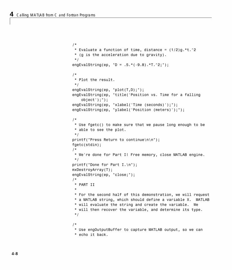
4 Calling MATLAB from C and Fortran Programs
4-8
/* * Evaluate a function of time, distance = (1/2)g.*t.^2 * (g is the acceleration due to gravity). */ engEvalString(ep, "D = .5.*(-9.8).*T.^2;");
/* * Plot the result. */ engEvalString(ep, "plot(T,D);"); engEvalString(ep, "title('Position vs. Time for a falling object');"); engEvalString(ep, "xlabel('Time (seconds)');"); engEvalString(ep, "ylabel('Position (meters)');");
/* * Use fgetc() to make sure that we pause long enough to be * able to see the plot. */ printf("Press Return to continue\n\n"); fgetc(stdin); /* * We're done for Part I! Free memory, close MATLAB engine. */ printf("Done for Part I.\n"); mxDestroyArray(T); engEvalString(ep, "close;"); /* * PART II * * For the second half of this demonstration, we will request * a MATLAB string, which should define a variable X. MATLAB * will evaluate the string and create the variable. We * will then recover the variable, and determine its type. */
/* * Use engOutputBuffer to capture MATLAB output, so we can * echo it back.
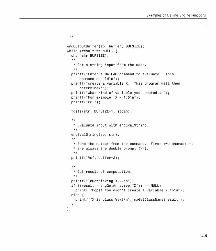
Examples of Calling Engine Functions
4-9
*/
engOutputBuffer(ep, buffer, BUFSIZE); while (result == NULL) { char str[BUFSIZE]; /* * Get a string input from the user. */ printf("Enter a MATLAB command to evaluate. This command should\n"); printf("create a variable X. This program will then determine\n"); printf("what kind of variable you created.\n"); printf("For example: X = 1:5\n"); printf(">> ");
fgets(str, BUFSIZE-1, stdin);
/* * Evaluate input with engEvalString. */ engEvalString(ep, str); /* * Echo the output from the command. First two characters * are always the double prompt (>>). */ printf("%s", buffer+2);
/* * Get result of computation. */ printf("\nRetrieving X...\n"); if ((result = engGetArray(ep,"X")) == NULL) printf("Oops! You didn't create a variable X.\n\n"); else { printf("X is class %s\t\n", mxGetClassName(result)); } }
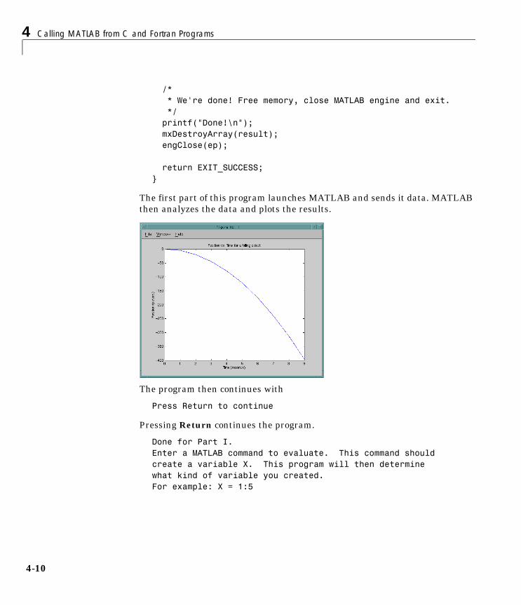
4 Calling MATLAB from C and Fortran Programs
4-10
/* * We're done! Free memory, close MATLAB engine and exit. */ printf("Done!\n"); mxDestroyArray(result); engClose(ep);
return EXIT_SUCCESS;}
The first part of this program launches MATLAB and sends it data. MATLAB then analyzes the data and plots the results.
The program then continues with
Press Return to continue
Pressing Return continues the program.
Done for Part I.Enter a MATLAB command to evaluate. This command shouldcreate a variable X. This program will then determinewhat kind of variable you created.For example: X = 1:5

Examples of Calling Engine Functions
4-11
Entering X = 17.5 continues the program execution.
X = 17.5 X = 17.5000 Retrieving X...X is class doubleDone!
Finally, the program frees memory, closes the MATLAB engine, and exits.
Calling MATLAB From a Fortran ApplicationThis program, fengdemo.f, illustrates how to call the engine functions from a stand-alone Fortran program.
CCC fengdemo.fCC This program illustrates how to call the MATLABC Engine functions from a Fortran program.CC Copyright (c) 1996-2000 by The MathWorks, Inc.C C===============================================================C $Revision: 1.7 $ program mainC---------------------------------------------------------------C (pointer) Replace integer by integer*8 on the DEC Alpha C platform.C integer engOpen, engGetMatrix, mxCreateFull, mxGetPr integer ep, T, D C---------------------------------------------------------------C

4 Calling MATLAB from C and Fortran Programs
4-12
C Other variable declarations here double precision time(10), dist(10) integer engPutMatrix, engEvalString, engClose integer temp, status data time / 1.0, 2.0, 3.0, 4.0, 5.0, 6.0, 7.0, 8.0, 9.0, 10.0 /C ep = engOpen('matlab ')C if (ep .eq. 0) then write(6,*) 'Can''t start MATLAB engine' stop endifC T = mxCreateFull(1, 10, 0) call mxSetName(T, 'T') call mxCopyReal8ToPtr(time, mxGetPr(T), 10)CCC Place the variable T into the MATLAB workspace.C status = engPutMatrix(ep, T)C if (status .ne. 0) then write(6,*) 'engPutMatrix failed' stop endifCCC Evaluate a function of time, distance = (1/2)g.*t.^2C (g is the acceleration due to gravity)C if (engEvalString(ep, 'D = .5.*(-9.8).*T.^2;') .ne. 0) then write(6,*) 'engEvalString failed' stop endifC
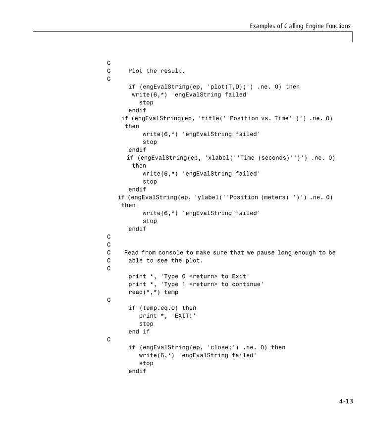
Examples of Calling Engine Functions
4-13
CC Plot the result.C if (engEvalString(ep, 'plot(T,D);') .ne. 0) then write(6,*) 'engEvalString failed' stop endif
if (engEvalString(ep, 'title(''Position vs. Time'')') .ne. 0) then
write(6,*) 'engEvalString failed' stop endif if (engEvalString(ep, 'xlabel(''Time (seconds)'')') .ne. 0)
then write(6,*) 'engEvalString failed' stop endif
if (engEvalString(ep, 'ylabel(''Position (meters)'')') .ne. 0) then
write(6,*) 'engEvalString failed' stop endifC C C Read from console to make sure that we pause long enough to beC able to see the plot.C print *, 'Type 0 <return> to Exit' print *, 'Type 1 <return> to continue' read(*,*) tempC if (temp.eq.0) then print *, 'EXIT!' stop end ifC if (engEvalString(ep, 'close;') .ne. 0) then write(6,*) 'engEvalString failed' stop endif
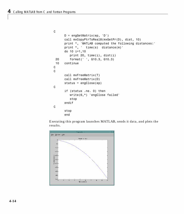
4 Calling MATLAB from C and Fortran Programs
4-14
C D = engGetMatrix(ep, 'D') call mxCopyPtrToReal8(mxGetPr(D), dist, 10) print *, 'MATLAB computed the following distances:' print *, ' time(s) distance(m)' do 10 i=1,10 print 20, time(i), dist(i) 20 format(' ', G10.3, G10.3) 10 continueCC call mxFreeMatrix(T) call mxFreeMatrix(D) status = engClose(ep)C if (status .ne. 0) then write(6,*) 'engClose failed' stop endifC stop end
Executing this program launches MATLAB, sends it data, and plots the results.
Examples of Calling Engine Functions
4-15
The program continues with
Type 0 <return> to ExitType 1 <return> to continue
Entering 1 at the prompt continues the program execution.
1 MATLAB computed the following distances: time(s) distance(m) 1.00 -4.90 2.00 -19.6 3.00 -44.1 4.00 -78.4 5.00 -123. 6.00 -176. 7.00 -240. 8.00 -314. 9.00 -397. 10.0 -490.
Finally, the program frees memory, closes the MATLAB engine, and exits.
Attaching to an Existing MATLAB SessionYou can make a MATLAB engine program attach to a MATLAB session that is already running by starting the MATLAB session with /Automation in the command line. When you make a call to engOpen, it will then connect to this existing session. You should only call engOpen once, as any engOpen calls will now connect to this one MATLAB session.
The /Automation option also causes the command window to be minimized. You must open it manually.
Note For more information on the /Automation command line argument and ActiveX in general, see “Introducing MATLAB ActiveX Integration” on page 7-3.
4 Calling MATLAB from C and Fortran Programs
4-16
For example:
1 Shut down any MATLAB sessions.
2 From the Start button on the Windows menu bar, click Run.
3 In the Open field, type
d:\matlab\bin\win32\matlab.exe /Automation
where d:\matlab\bin\win32 represents the path to the MATLAB executable.
4 Click OK. This starts MATLAB.
5 In MATLAB, change directories to $MATLAB/extern/examples/eng_mat, where $MATLAB is the MATLAB root directory.
6 Compile the engwindemo.c example.
7 Run the engwindemo program by typing at the MATLAB prompt
!engwindemo
This does not start another MATLAB session, but rather uses the MATLAB session that is already open.
Note On the UNIX platform, you cannot make a MATLAB engine program use a MATLAB session that is already running.
Compiling and Linking Engine Programs
4-17
Compiling and Linking Engine ProgramsTo produce an executable version of an engine program, you must compile it and link it with the appropriate library. This section describes the steps required to compile and link engine programs on UNIX and Windows systems. It begins by looking at a special consideration for compilers that do not mask floating-point exceptions. Topics covered are:
• “Masking Floating-Point Exceptions”
• “Compiling and Linking on UNIX”
• “Compiling and Linking on Windows”
Masking Floating-Point ExceptionsCertain mathematical operations can result in nonfinite values. For example, division by zero results in the nonfinite IEEE value, inf. A floating-point exception occurs when such an operation is performed. Because MATLAB uses an IEEE model that supports nonfinite values such as inf and NaN, MATLAB disables, or masks, floating-point exceptions.
Some compilers do not mask floating-point exceptions by default. This causes engine programs built with such compilers to terminate when a floating-point exception occurs. Consequently, you need to take special precautions when using these compilers to mask floating-point exceptions so that your engine application will perform properly.
Note MATLAB based applications should never get floating-point exceptions. If you do get a floating-point exception, verify that any third party libraries that you link against do not enable floating-point exception handling.
The only compiler and platform on which you need to mask floating-point exceptions is the Borland C++ compiler on Windows.
Borland C++ Compiler on WindowsTo mask floating-point exceptions when using the Borland C++ compiler on the Windows platform, you must add some code to your program. Include the following at the beginning of your main() or WinMain() function, before any calls to MATLAB API functions.
4 Calling MATLAB from C and Fortran Programs
4-18
#include <float.h>...
_control87(MCW_EM,MCW_EM);...
Compiling and Linking on UNIXUnder UNIX at runtime, you must tell the system where the API shared libraries reside. These sections provide the necessary UNIX commands depending on your shell and system architecture.
Setting Runtime Library PathIn C shell, the command to set the library path is
setenv LD_LIBRARY_PATH <matlab>/extern/lib/$Arch:$LD_LIBRARY_PATH
In Bourne shell, the commands to set the library path are
LD_LIBRARY_PATH=<matlab>/extern/lib/$Arch:$LD_LIBRARY_PATHexport LD_LIBRARY_PATH
where <matlab> is the MATLAB root directory and $Arch is your system architecture (alpha, glnx86, sgi, sol2, hp700, or ibm_rs).
Note that the environment variable (LD_LIBRARY_PATH in this example) varies on several platforms. This table lists the different environment variable names you should use on these systems.
It is convenient to place these commands in a startup script such as ~/.cshrc for C shell or ~/.profile for Bourne shell.
Table 4-3: Environment Variable Names
Architecture Environment Variable
HP700 SHLIB_PATH
IBM RS/6000 LIBPATH
Compiling and Linking Engine Programs
4-19
Compiling and LinkingMATLAB provides an options file, engopts.sh, that lets you use the mex script to easily compile and link engine applications. For example, to compile and link the engdemo.c example, you can use
mex -f <matlab>/bin/engopts.sh <pathname>/engdemo.c
where <pathname> specifies the complete path to the specified file.
If you need to modify the options file for your particular compiler or platform, use the -v switch to view the current compiler and linker settings and then make the appropriate changes in a local copy of the engopts.sh file.
Compiling and Linking on WindowsTo compile and link engine programs, use the mex script with an engine options file. Table 1-2, Options Files, on page 1-17 lists the engine options files included in this release. All of these options files are located in <matlab>\bin\win32\mexopts.
As an example, to compile and link the stand-alone engine application engwindemo.c on Windows using MSVC (Version 5.0), use
mex -f <matlab>\bin\win32\mexopts\msvc50engmatopts.bat ... <pathname>\engwindemo.c
where <pathname> specifies the complete path to the specified file. If you need to modify the options file for your particular compiler, use the -v switch to view the current compiler and linker settings and then make the appropriate changes in the options file.

4 Calling MATLAB from C and Fortran Programs
4-20
5Calling Java from MATLAB
Using Java from MATLAB: An Overview . . . . . . . 5-3
Bringing Java Classes into MATLAB . . . . . . . . . 5-5
Creating and Using Java Objects . . . . . . . . . . 5-10
Invoking Methods on Java Objects . . . . . . . . . . 5-19
Working with Java Arrays . . . . . . . . . . . . . 5-29
Passing Data to a Java Method . . . . . . . . . . . 5-46
Handling Data Returned from a Java Method . . . . . 5-56
Introduction to Programming Examples . . . . . . . 5-62
Example – Reading a URL . . . . . . . . . . . . . . 5-63
Example – Finding an Internet Protocol Address . . . 5-66
Example – Communicating Through a Serial Port . . . 5-68
Example – Creating and Using a Phone Book . . . . . 5-73
5 Calling Java from MATLAB
5-2
This chapter describes how to use the MATLAB interface to Java classes and objects. This MATLAB capability enables you to conveniently bring Java classes into the MATLAB environment, to construct objects from those classes, to call methods on the Java objects, and to save Java objects for later reloading — all accomplished with MATLAB functions and commands.
The following list summarizes the contents of this chapter:
• “Using Java from MATLAB: An Overview”
• “Bringing Java Classes into MATLAB”
• “Creating and Using Java Objects”
• “Invoking Methods on Java Objects”
• “Working with Java Arrays”
• “Passing Data to a Java Method”
• “Handling Data Returned from a Java Method”
• “Introduction to Programming Examples”
Using Java from MATLAB: An Overview
5-3
Using Java from MATLAB: An Overview
Java Interface Is Integral to MATLABEvery installation of MATLAB includes a Java Virtual Machine (JVM), so that you can use the Java interpreter via MATLAB commands, and you can create and run programs that create and access Java objects. For information on MATLAB installation, see the MATLAB installation documentation for your platform.
Benefits of the MATLAB Java InterfaceThe MATLAB Java interface enables you to:
• Access Java API (application programming interface) class packages that support essential activities such as I/O and networking. For example, the URL class provides convenient access to resources on the internet
• Access third-party Java classes
• Easily construct Java objects in MATLAB
• Call Java object methods, using either Java or MATLAB syntax
• Pass data between MATLAB variables and Java objects
Who Should Use the MATLAB Java InterfaceThe MATLAB Java interface is intended for all MATLAB users who want to take advantage of the special capabilities of the Java programming language. For example:
• You need to access, from MATLAB, the capabilities of available Java classes.
• You are familiar with object-oriented programming in Java or in another language, such as C++.
• You are familiar with MATLAB object-oriented classes, or with MATLAB MEX-files.
To Learn More About Java ProgrammingFor a complete description of the Java language and for guidance in object-oriented software design and programming, you’ll need to consult outside resources. For example, these recently published books may be helpful:

5 Calling Java from MATLAB
5-4
• Java in a Nutshell (Second Edition), by David Flanagan
• Teach Yourself Java in 21 Days, by Lemay and Perkins
Another place to find information is the JavaSoft Web site.
http://www.javasoft.com
For other suggestions on object-oriented programming resources, see:
• Object Oriented Software Construction, by Bertrand Meyer
• Object Oriented Analysis and Design with Applications, by Grady Booch
Platform Support for the Java Virtual MachineTo find out which version of the Java Virtual Machine (JVM) is being used by MATLAB on your platform, type the following at the MATLAB prompt.
version -java
Bringing Java Classes into MATLAB
5-5
Bringing Java Classes into MATLABYou can draw from an extensive collection of existing Java classes or create your own class definitions to use with MATLAB. This section explains how to go about finding the class definitions that you need or how to create classes of your own design. Once you have the classes you need, defined in either individual .class files, packages, or Java Archive files, you will see how to make them available within the MATLAB environment.
This section addresses the following topics:
• “Sources of Java Classes”
• “Defining New Java Classes”
• “Making Java Classes Available to MATLAB”
• “Loading Java Class Definitions”
• “Simplifying Java Class Names”
Sources of Java ClassesThere are three main sources of Java classes that you can use in MATLAB:
• Java built-in classes
The Java language includes general-purpose class packages, such as java.awt. See your Java language documentation for descriptions of these packages.
• Third-party classes
There are a number of packages of special-purpose Java classes that you can use.
• User-defined classes
You can define new Java classes or subclasses of existing classes. You need to use a Java development environment to do this, as explained in the following section.
Defining New Java ClassesTo define new Java classes and subclasses of existing classes, you must use a Java development environment, external to MATLAB, that supports Java version 1.1. You can download the development kit that supports the version
5 Calling Java from MATLAB
5-6
1.1.8 Java Virtual Machine from the web site at Sun Microsystems, (http://www.java.sun.com/jdk/). The Sun site also provides documentation for the Java language and classes that you will need for development.
After you create class definitions in .java files, use your Java compiler to produce .class files from them. The next step is to make the class definitions in those .class files available for you to use in MATLAB.
Making Java Classes Available to MATLABTo make your third-party and user-defined Java classes available in MATLAB, place them on your MATLAB path by adding their locations to the file classpath.txt. For more information on classpath.txt, see “Finding and Editing classpath.txt” on page 5-7.
Making Individual (Unpackaged) Classes AvailableTo make individual classes (classes not part of a package) available in MATLAB, add to classpath.txt an entry containing the full path to the directory you want to use for the .class file(s).
For example, to make available your compiled Java classes in the file d:\work\javaclasses\test.class, add the following entry to your classpath.txt file.
d:\work\javaclasses
Making Entire Packages AvailableTo access one or more classes belonging to a package, you need to make the entire package available to MATLAB. Do this by adding to classpath.txt the full path to the parent directory of the highest-level directory of the package path. This directory is the first component in the package name.
For example, if your Java class package com.mw.tbx.ini has its classes in directory d:\work\com\mw\tbx\ini, add the following entry to your classpath.txt.
d:\work
Making Classes in a JAR File AvailableYou can use the jar (Java Archive) tool to create a JAR file, containing multiple Java classes and packages in a compressed ZIP format. For information on jar
Bringing Java Classes into MATLAB
5-7
and JAR files, consult your Java development documentation or the JavaSoft web site. See also “To Learn More About Java Programming” on page 5-3.
To make the contents of a JAR file available for use in MATLAB, add to classpath.txt the full path, including full filename, for the JAR file.
Note Note that the classpath.txt requirement for JAR files is different than that for .class files and packages, for which you do not specify any filename.
For example, to make available the JAR file e:\java\classes\utilpkg.jar, add the following to your classpath.txt.
e:\java\classes\utilpkg.jar
Finding and Editing classpath.txtTo make your Java classes available, you can edit the default classpath.txt, which is in the directory toolbox/local. Or, you can copy the default classpath.txt from this directory to your own startup directory where the changes you make to it do not affect anyone else.
To find the classpath.txt that is used by your MATLAB environment, use the MATLAB which function.
which classpath.txt
To edit either the default file or the copy you have made in your own directory, enter the following command in MATLAB.
edit classpath.txt
MATLAB reads classpath.txt only upon startup. So, if you edit classpath.txt or change your .class files while MATLAB is running, you must restart MATLAB to put those changes into effect.
Loading Java Class DefinitionsNormally, MATLAB loads a Java class automatically when your code first uses it, (for example, when you call its constructor). However, there is one exception that you should be aware of.
5 Calling Java from MATLAB
5-8
When you use the which function on methods defined by Java classes, the function only acts on the classes currently loaded into the MATLAB working environment. In contrast, which always operates on MATLAB classes, whether or not they are loaded.
Determining Which Classes Are LoadedAt any time during a MATLAB session, you can obtain a listing of all the Java classes that are currently loaded. To do so, you use the inmem function, in the following form.
[M,X,J] = inmem
This function returns the list of Java classes in output argument J. (It also returns in M the names of all currently loaded M-files, and in X the names of all currently loaded MEX-files.)
Here’s a sample of output from the inmem function.
[m,x,j] = inmemm =
'isequal''isunix''fullfile''filesep'...'matlabrc'
x = 'getprofl'
j = 'java.awt.Frame''com.mathworks.ide.desktop.MLDesktop'
Simplifying Java Class NamesYour MATLAB commands can refer to any Java class by its fully qualified name, which includes its package name. For example, the following are fully qualified names:
Bringing Java Classes into MATLAB
5-9
• java.lang.String• java.util.Enumeration
A fully qualified name can be rather long, making commands and functions, such as constructors, cumbersome to edit and to read. You can refer to classes by the class name alone (without a package name) if you, first, import the fully qualified name into MATLAB.
The import command has the following forms.
import pkg_name.* % Import all classes in packageimport pkg_name1.* pkg_name2.* % Import multiple packagesimport class_name % Import one classimport % Display current import listL = import % Return current import list
MATLAB adds all classes that you import to a list called the import list. You can see what classes are on that list by typing import, without any arguments. Your code can refer to any class on the list by class name alone.
When called from a function, import adds the specified classes to the import list in effect for that function. When invoked at the command prompt, import uses the base import list for your MATLAB environment.
For example, suppose a function contains the following statements.
import java.lang.Stringimport java.util.* java.awt.*import java.util.Enumeration
Code that follows the import statements above can now refer to the String, Frame, and Enumeration classes without using the package names.
str = String('hello'); % Create java.lang.String objectfrm = Frame; % Create java.awt.Frame objectmethods Enumeration % List java.util.Enumeration methods
To clear the list of imported Java classes, invoke the command
clear import
5 Calling Java from MATLAB
5-10
Creating and Using Java ObjectsIn MATLAB, you create a Java object by calling one of the constructors of that class. You then use commands and programming statements to perform operations on these objects. You can also save your Java objects to a MAT-file and, in subsequent sessions, reload them into MATLAB.
This section addresses the following topics:
• “Constructing Java Objects”
• “Concatenating Java Objects”
• “Saving and Loading Java Objects to MAT-Files”
• “Finding the Public Data Fields of an Object”
• “Accessing Private and Public Data”
• “Determining the Class of an Object”
Constructing Java ObjectsYou construct Java objects in MATLAB by calling the Java class constructor, which has the same name as the class. For example, the following constructor creates a Frame object with the title 'Frame A' and the other properties with their default values.
frame = java.awt.Frame('Frame A');
Displaying the new object frame shows the following.
frame = java.awt.Frame[frame0,0,0,0x0,invalid,hidden,layout=java.awt.BorderLayout,resizable,title=Frame A]
All of the programming examples in this chapter contain Java object constructors. For example, the sample code for Reading a URL creates a java.net.URL object with the constructor
url = java.net.URL(... 'http://www.ncsa.uiuc.edu/demoweb/url-primer.html')
Using the javaObject FunctionUnder certain circumstances, you may need to use the javaObject function to construct a Java object. The following syntax invokes the Java constructor for

Creating and Using Java Objects
5-11
class, class_name, with the argument list that matches x1,...,xn, and returns a new object, J.
J = javaObject('class_name',x1,...,xn);
For example, to construct and return a Java object of class java.lang.String, you use
strObj = javaObject('java.lang.String','hello');
Using the javaObject function enables you to:
• Use classes having names with more than 31 consecutive characters
• Specify the class for an object at run-time, for example, as input from an application user
The default MATLAB constructor syntax requires that no segment of the input class name be longer than 31 characters. (A class name segment is any portion of the class name before, between, or after a dot. For example, there are three segments in class, java.lang.String.) Any class name segment that exceeds 31 characters is truncated by MATLAB. In the rare case where you need to use a class name of this length, you must use javaObject to instantiate the class.
The javaObject function also allows you to specify the Java class for the object being constructed at run-time. In this situation, you call javaObject with a string variable in place of the class name argument.
class = 'java.lang.String';text = 'hello';strObj = javaObject(class, text);
In the usual case, when the class to instantiate is known at development time, it is more convenient to use the MATLAB constructor syntax. For example, to create a java.lang.String object, you would use
strObj = java.lang.String('hello');
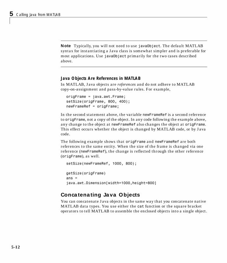
5 Calling Java from MATLAB
5-12
Note Typically, you will not need to use javaObject. The default MATLAB syntax for instantiating a Java class is somewhat simpler and is preferable for most applications. Use javaObject primarily for the two cases described above.
Java Objects Are References in MATLABIn MATLAB, Java objects are references and do not adhere to MATLAB copy-on-assignment and pass-by-value rules. For example,
origFrame = java.awt.Frame;setSize(origFrame, 800, 400);newFrameRef = origFrame;
In the second statement above, the variable newFrameRef is a second reference to origFrame, not a copy of the object. In any code following the example above, any change to the object at newFrameRef also changes the object at origFrame. This effect occurs whether the object is changed by MATLAB code, or by Java code.
The following example shows that origFrame and newFrameRef are both references to the same entity. When the size of the frame is changed via one reference (newFrameRef), the change is reflected through the other reference (origFrame), as well.
setSize(newFrameRef, 1000, 800);
getSize(origFrame)ans =java.awt.Dimension[width=1000,height=800]
Concatenating Java ObjectsYou can concatenate Java objects in the same way that you concatenate native MATLAB data types. You use either the cat function or the square bracket operators to tell MATLAB to assemble the enclosed objects into a single object.
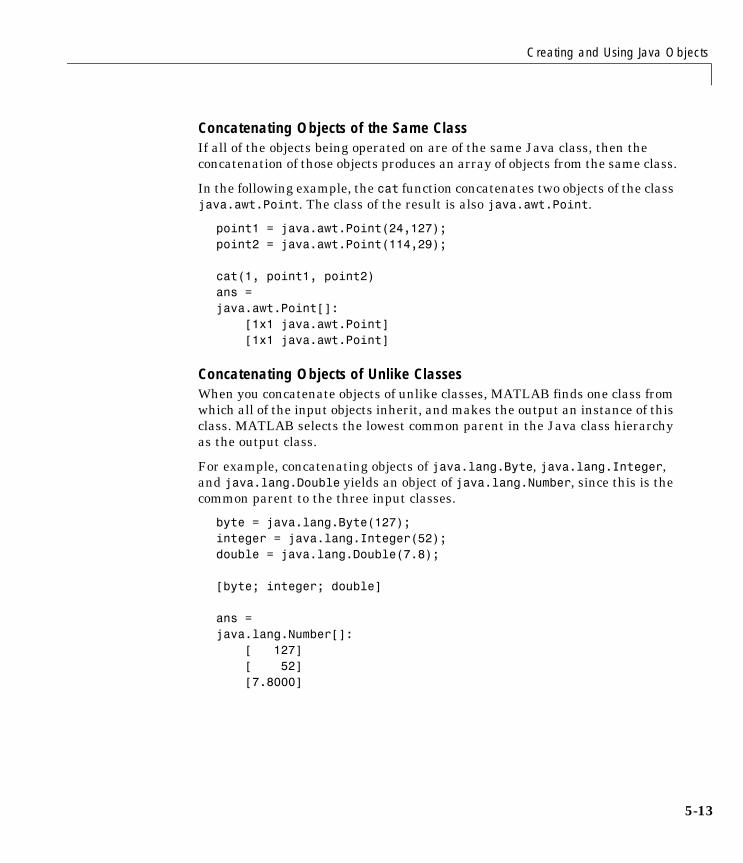
Creating and Using Java Objects
5-13
Concatenating Objects of the Same ClassIf all of the objects being operated on are of the same Java class, then the concatenation of those objects produces an array of objects from the same class.
In the following example, the cat function concatenates two objects of the class java.awt.Point. The class of the result is also java.awt.Point.
point1 = java.awt.Point(24,127);point2 = java.awt.Point(114,29);
cat(1, point1, point2)ans = java.awt.Point[]: [1x1 java.awt.Point] [1x1 java.awt.Point]
Concatenating Objects of Unlike ClassesWhen you concatenate objects of unlike classes, MATLAB finds one class from which all of the input objects inherit, and makes the output an instance of this class. MATLAB selects the lowest common parent in the Java class hierarchy as the output class.
For example, concatenating objects of java.lang.Byte, java.lang.Integer, and java.lang.Double yields an object of java.lang.Number, since this is the common parent to the three input classes.
byte = java.lang.Byte(127);integer = java.lang.Integer(52);double = java.lang.Double(7.8);
[byte; integer; double]
ans =java.lang.Number[]: [ 127] [ 52] [7.8000]
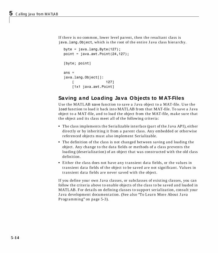
5 Calling Java from MATLAB
5-14
If there is no common, lower level parent, then the resultant class is java.lang.Object, which is the root of the entire Java class hierarchy.
byte = java.lang.Byte(127);point = java.awt.Point(24,127);
[byte; point]
ans =java.lang.Object[]: [ 127] [1x1 java.awt.Point]
Saving and Loading Java Objects to MAT-FilesUse the MATLAB save function to save a Java object to a MAT-file. Use the load function to load it back into MATLAB from that MAT-file. To save a Java object to a MAT-file, and to load the object from the MAT-file, make sure that the object and its class meet all of the following criteria:
• The class implements the Serializable interface (part of the Java API), either directly or by inheriting it from a parent class. Any embedded or otherwise referenced objects must also implement Serializable.
• The definition of the class is not changed between saving and loading the object. Any change to the data fields or methods of a class prevents the loading (deserialization) of an object that was constructed with the old class definition.
• Either the class does not have any transient data fields, or the values in transient data fields of the object to be saved are not significant. Values in transient data fields are never saved with the object.
If you define your own Java classes, or subclasses of existing classes, you can follow the criteria above to enable objects of the class to be saved and loaded in MATLAB. For details on defining classes to support serialization, consult your Java development documentation. (See also “To Learn More About Java Programming” on page 5-3).
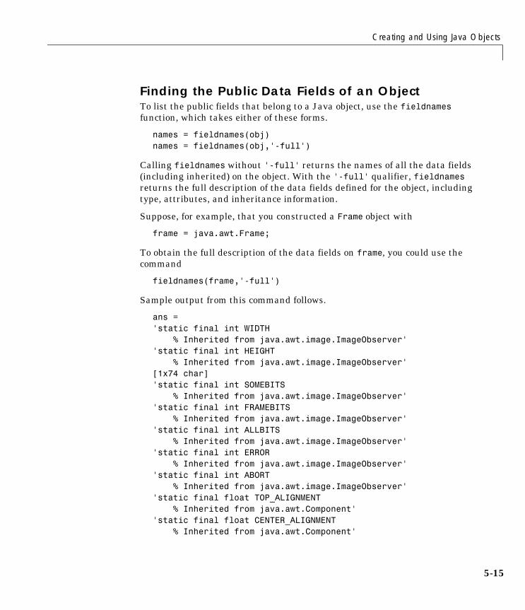
Creating and Using Java Objects
5-15
Finding the Public Data Fields of an ObjectTo list the public fields that belong to a Java object, use the fieldnames function, which takes either of these forms.
names = fieldnames(obj)names = fieldnames(obj,'-full')
Calling fieldnames without '-full' returns the names of all the data fields (including inherited) on the object. With the '-full' qualifier, fieldnames returns the full description of the data fields defined for the object, including type, attributes, and inheritance information.
Suppose, for example, that you constructed a Frame object with
frame = java.awt.Frame;
To obtain the full description of the data fields on frame, you could use the command
fieldnames(frame,'-full')
Sample output from this command follows.
ans = 'static final int WIDTH % Inherited from java.awt.image.ImageObserver''static final int HEIGHT % Inherited from java.awt.image.ImageObserver'[1x74 char]'static final int SOMEBITS % Inherited from java.awt.image.ImageObserver''static final int FRAMEBITS % Inherited from java.awt.image.ImageObserver''static final int ALLBITS % Inherited from java.awt.image.ImageObserver''static final int ERROR % Inherited from java.awt.image.ImageObserver''static final int ABORT % Inherited from java.awt.image.ImageObserver''static final float TOP_ALIGNMENT % Inherited from java.awt.Component''static final float CENTER_ALIGNMENT % Inherited from java.awt.Component'
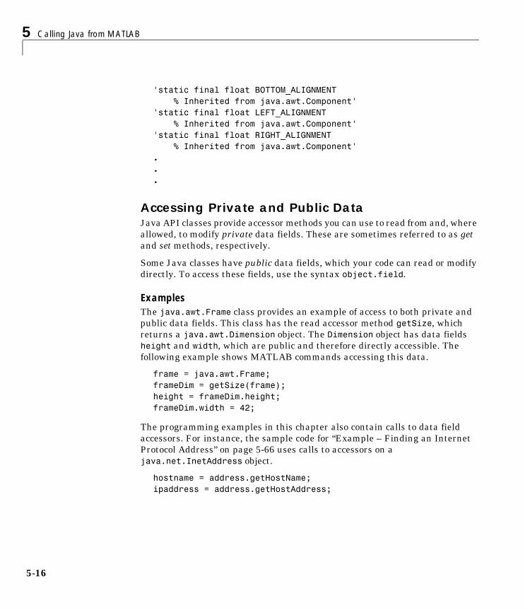
5 Calling Java from MATLAB
5-16
'static final float BOTTOM_ALIGNMENT % Inherited from java.awt.Component''static final float LEFT_ALIGNMENT % Inherited from java.awt.Component''static final float RIGHT_ALIGNMENT % Inherited from java.awt.Component'...
Accessing Private and Public DataJava API classes provide accessor methods you can use to read from and, where allowed, to modify private data fields. These are sometimes referred to as get and set methods, respectively.
Some Java classes have public data fields, which your code can read or modify directly. To access these fields, use the syntax object.field.
ExamplesThe java.awt.Frame class provides an example of access to both private and public data fields. This class has the read accessor method getSize, which returns a java.awt.Dimension object. The Dimension object has data fields height and width, which are public and therefore directly accessible. The following example shows MATLAB commands accessing this data.
frame = java.awt.Frame;frameDim = getSize(frame);height = frameDim.height;frameDim.width = 42;
The programming examples in this chapter also contain calls to data field accessors. For instance, the sample code for “Example – Finding an Internet Protocol Address” on page 5-66 uses calls to accessors on a java.net.InetAddress object.
hostname = address.getHostName; ipaddress = address.getHostAddress;
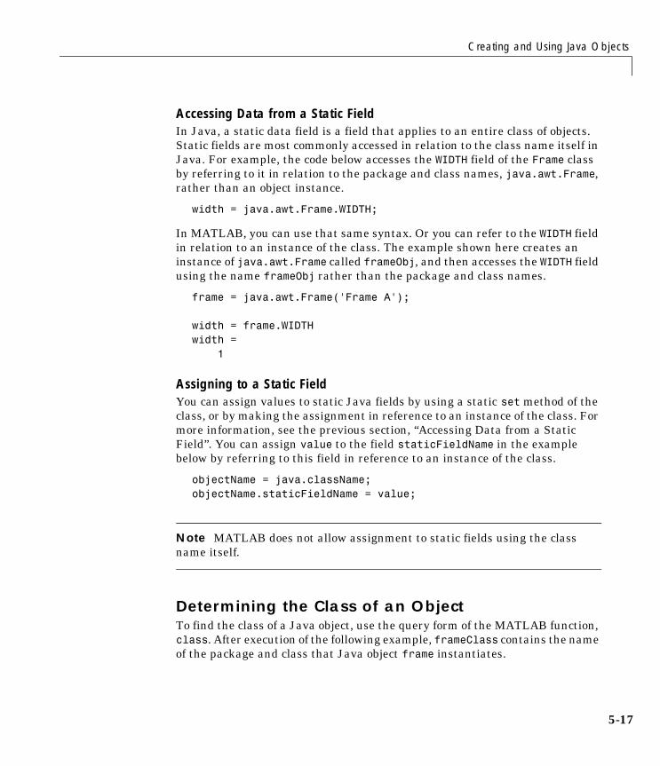
Creating and Using Java Objects
5-17
Accessing Data from a Static FieldIn Java, a static data field is a field that applies to an entire class of objects. Static fields are most commonly accessed in relation to the class name itself in Java. For example, the code below accesses the WIDTH field of the Frame class by referring to it in relation to the package and class names, java.awt.Frame, rather than an object instance.
width = java.awt.Frame.WIDTH;
In MATLAB, you can use that same syntax. Or you can refer to the WIDTH field in relation to an instance of the class. The example shown here creates an instance of java.awt.Frame called frameObj, and then accesses the WIDTH field using the name frameObj rather than the package and class names.
frame = java.awt.Frame('Frame A');
width = frame.WIDTHwidth = 1
Assigning to a Static FieldYou can assign values to static Java fields by using a static set method of the class, or by making the assignment in reference to an instance of the class. For more information, see the previous section, “Accessing Data from a Static Field”. You can assign value to the field staticFieldName in the example below by referring to this field in reference to an instance of the class.
objectName = java.className;objectName.staticFieldName = value;
Note MATLAB does not allow assignment to static fields using the class name itself.
Determining the Class of an ObjectTo find the class of a Java object, use the query form of the MATLAB function, class. After execution of the following example, frameClass contains the name of the package and class that Java object frame instantiates.
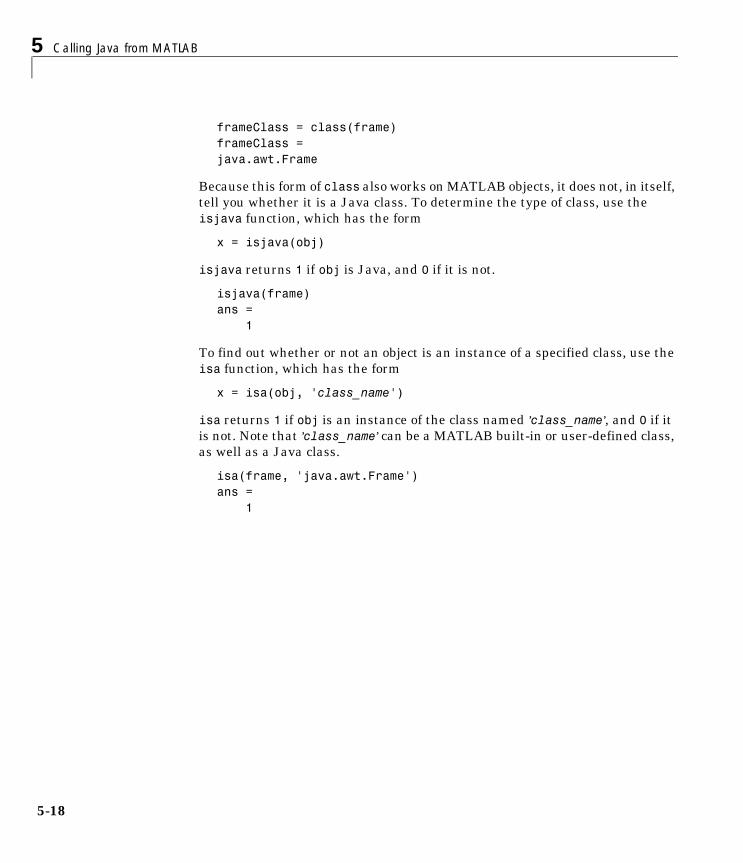
5 Calling Java from MATLAB
5-18
frameClass = class(frame)frameClass = java.awt.Frame
Because this form of class also works on MATLAB objects, it does not, in itself, tell you whether it is a Java class. To determine the type of class, use the isjava function, which has the form
x = isjava(obj)
isjava returns 1 if obj is Java, and 0 if it is not.
isjava(frame)ans = 1
To find out whether or not an object is an instance of a specified class, use the isa function, which has the form
x = isa(obj, 'class_name')
isa returns 1 if obj is an instance of the class named ’class_name’, and 0 if it is not. Note that ’class_name’ can be a MATLAB built-in or user-defined class, as well as a Java class.
isa(frame, 'java.awt.Frame')ans = 1
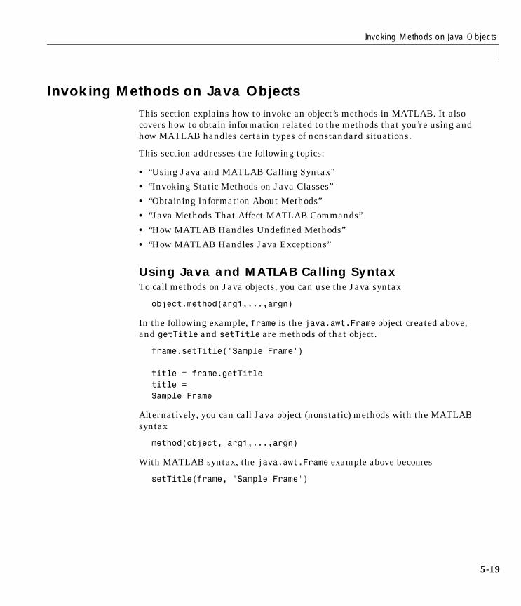
Invoking Methods on Java Objects
5-19
Invoking Methods on Java ObjectsThis section explains how to invoke an object’s methods in MATLAB. It also covers how to obtain information related to the methods that you’re using and how MATLAB handles certain types of nonstandard situations.
This section addresses the following topics:
• “Using Java and MATLAB Calling Syntax”
• “Invoking Static Methods on Java Classes”
• “Obtaining Information About Methods”
• “Java Methods That Affect MATLAB Commands”
• “How MATLAB Handles Undefined Methods”
• “How MATLAB Handles Java Exceptions”
Using Java and MATLAB Calling SyntaxTo call methods on Java objects, you can use the Java syntax
object.method(arg1,...,argn)
In the following example, frame is the java.awt.Frame object created above, and getTitle and setTitle are methods of that object.
frame.setTitle('Sample Frame')
title = frame.getTitletitle = Sample Frame
Alternatively, you can call Java object (nonstatic) methods with the MATLAB syntax
method(object, arg1,...,argn)
With MATLAB syntax, the java.awt.Frame example above becomes
setTitle(frame, 'Sample Frame')
5 Calling Java from MATLAB
5-20
title = getTitle(frame)title = Sample Frame
All of the programming examples in this chapter contain invocations of Java object methods. For example, the code for Reading a URL contains a call, using MATLAB syntax, to the openStream method on a java.net.URL object, url.
is = openStream(url)
In another example, the code for “Example – Creating and Using a Phone Book” on page 5-73 contains a call, using Java syntax, to the load method on a java.utils.Properties object, pb_htable.
pb_htable.load(FIS);
Using the javaMethod Function on Nonstatic MethodsUnder certain circumstances, you may need to use the javaMethod function to call a Java method. The following syntax invokes the method, method_name, on Java object J with the argument list that matches x1,...,xn. This returns the value X.
X = javaMethod('method_name',J,x1,...,xn);
For example, to call the startsWith method on a java.lang.String object passing one argument, use
gAddress = java.lang.String('Four score and seven years ago');str = java.lang.String('Four score');
javaMethod('startsWith', gAddress, str)ans = 1
Using the javaMethod function enables you to:
• Use methods having names longer than 31 characters
• Specify the method you want to invoke at run-time, for example, as input from an application user
The only way to invoke a method whose name is longer than 31 characters is to use javaMethod. The Java and MATLAB calling syntax does not accept method names of this length.
Invoking Methods on Java Objects
5-21
With javaMethod, you can also specify the method to be invoked at run-time. In this situation, your code calls javaMethod with a string variable in place of the method name argument. When you use javaMethod to invoke a static method, you can also use a string variable in place of the class name argument.
Note Typically, you will not need to use javaMethod. The default MATLAB syntax for invoking a Java method is somewhat simpler and is preferable for most applications. Use javaMethod primarily for the two cases described above.
Invoking Static Methods on Java ClassesTo invoke a static method on a Java class, use the Java invocation syntax
class.method(arg1,...,argn)
For example, call the isNaN static method on the java.lang.Double class.
java.lang.Double.isNaN(2.2)
Alternatively, you can apply static method names to instances of a class. In this example, the isNaN static method is referenced in relation to the dblObject instance of the java.lang.Double class.
dblObject = java.lang.Double(2.2);
dblObject.isNaNans = 0
Several of the programming examples in this chapter contain examples of static method invocation. For example, the code for Communicating Through a Serial Port contains a call to static method getPortIdentifier on Java class javax.comm.CommPortIdentifier.
commPort = javax.comm.CommPortIdentifier.getPortIdentifier('COM1');
5 Calling Java from MATLAB
5-22
Using the javaMethod Function on Static MethodsThe javaMethod function was introduced in section “Using the javaMethod Function on Nonstatic Methods” on page 5-20. You can also use this function to call static methods.
The following syntax invokes the static method, method_name, in class, class_name, with the argument list that matches x1,...,xn. This returns the value X.
X = javaMethod('method_name','class_name',x1,...,xn);
For example, to call the static isNaN method of the java.lang.Double class on a double value of 2.2, you use
javaMethod('isNaN','java.lang.Double',2.2);
Using the javaMethod function to call static methods enables you to:
• Use methods having names longer than 31 characters
• Specify method and class names at run-time, for example, as input from an application user
Obtaining Information About MethodsMATLAB offers several functions to help obtain information related to the Java methods you are working with. You can request a list of all of the methods that are implemented by any class. The list may be accompanied by other method information such as argument types and exceptions. You can also request a listing of every Java class that you loaded into MATLAB that implements a specified method.
Methodsview: Displaying a Listing of Java MethodsIf you want to know what methods are implemented by a particular Java (or MATLAB) class, use the methodsview function in MATLAB. Specify the class name (along with its package name, for Java classes) in the command line. If you have imported the package that defines this class, then the class name alone will suffice.
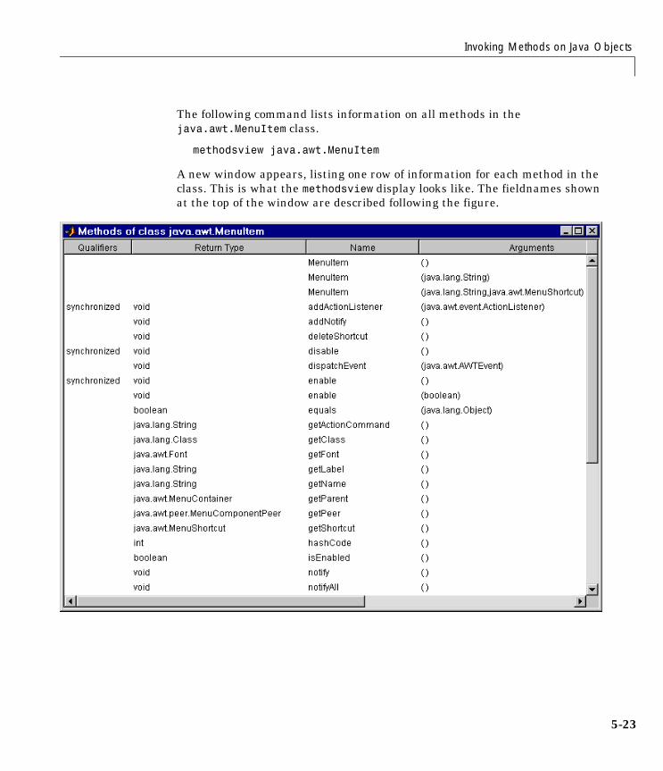
Invoking Methods on Java Objects
5-23
The following command lists information on all methods in the java.awt.MenuItem class.
methodsview java.awt.MenuItem
A new window appears, listing one row of information for each method in the class. This is what the methodsview display looks like. The fieldnames shown at the top of the window are described following the figure.
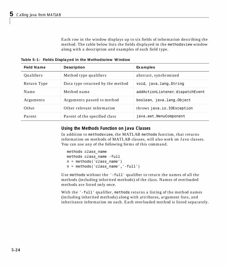
5 Calling Java from MATLAB
5-24
Each row in the window displays up to six fields of information describing the method. The table below lists the fields displayed in the methodsview window along with a description and examples of each field type.
Using the Methods Function on Java ClassesIn addition to methodsview, the MATLAB methods function, that returns information on methods of MATLAB classes, will also work on Java classes. You can use any of the following forms of this command.
methods class_namemethods class_name -fulln = methods('class_name')n = methods('class_name','-full')
Use methods without the '-full' qualifier to return the names of all the methods (including inherited methods) of the class. Names of overloaded methods are listed only once.
With the '-full' qualifier, methods returns a listing of the method names (including inherited methods) along with attributes, argument lists, and inheritance information on each. Each overloaded method is listed separately.
Table 5-1: Fields Displayed in the Methodsview Window
Field Name Description Examples
Qualifiers Method type qualifiers abstract, synchronized
Return Type Data type returned by the method void, java.lang.String
Name Method name addActionListener, dispatchEvent
Arguments Arguments passed to method boolean, java.lang.Object
Other Other relevant information throws java.io.IOException
Parent Parent of the specified class java.awt.MenuComponent
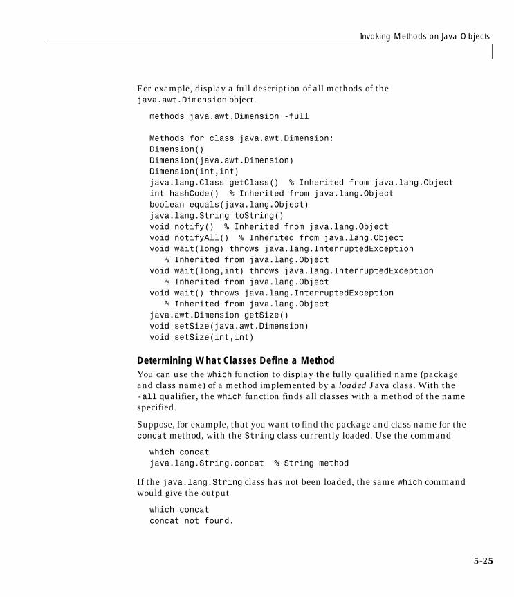
Invoking Methods on Java Objects
5-25
For example, display a full description of all methods of the java.awt.Dimension object.
methods java.awt.Dimension -full
Methods for class java.awt.Dimension:Dimension() Dimension(java.awt.Dimension) Dimension(int,int) java.lang.Class getClass() % Inherited from java.lang.Object int hashCode() % Inherited from java.lang.Object boolean equals(java.lang.Object) java.lang.String toString() void notify() % Inherited from java.lang.Object void notifyAll() % Inherited from java.lang.Object void wait(long) throws java.lang.InterruptedException % Inherited from java.lang.Objectvoid wait(long,int) throws java.lang.InterruptedException % Inherited from java.lang.Object void wait() throws java.lang.InterruptedException % Inherited from java.lang.Object java.awt.Dimension getSize() void setSize(java.awt.Dimension) void setSize(int,int)
Determining What Classes Define a MethodYou can use the which function to display the fully qualified name (package and class name) of a method implemented by a loaded Java class. With the -all qualifier, the which function finds all classes with a method of the name specified.
Suppose, for example, that you want to find the package and class name for the concat method, with the String class currently loaded. Use the command
which concatjava.lang.String.concat % String method
If the java.lang.String class has not been loaded, the same which command would give the output
which concatconcat not found.
5 Calling Java from MATLAB
5-26
If you use which -all for the method equals, with the String and java.awt.Frame classes loaded, you see the following display.
which -all equalsjava.lang.String.equals % String methodjava.awt.Frame.equals % Frame methodcom.mathworks.ide.desktop.MLDesktop.equals % MLDesktop method
The which function operates differently on Java classes than it does on MATLAB classes. MATLAB classes are always displayed by which, whether or not they are loaded. This is not true for Java classes. You can find out which Java classes are currently loaded by using the command [m,x,j]=inmem, described in “Determining Which Classes Are Loaded” on page 5-8.
For a description of how Java classes are loaded, see “Making Java Classes Available to MATLAB” on page 5-6.
Java Methods That Affect MATLAB CommandsMATLAB commands that operate on Java objects and arrays make use of the methods that are implemented within, or inherited by, these objects’ classes. There are some MATLAB commands that you can alter somewhat in behavior by changing the Java methods that they rely on.
Changing the Effect of disp and displayYou can use the disp function to display the value of a variable or an expression in MATLAB. Terminating a command line without a semicolon also calls the disp function. You can also use disp to display a Java object in MATLAB.
When disp operates on a Java object, MATLAB formats the output using the toString method of the class to which the object belongs. If the class does not implement this method, then an inherited toString method is used. If no intermediate ancestor classes define this method, it uses the toString method defined by the java.lang.Object class. You can override inherited toString methods in classes that you create by implementing such a method within your class definition. In this way, you can change the way MATLAB displays information regarding the objects of the class.
Invoking Methods on Java Objects
5-27
Changing the Effect of isequalThe MATLAB isequal function compares two or more arrays for equality in type, size, and contents. This function can also be used to test Java objects for equality.
When you compare two Java objects using isequal, MATLAB performs the comparison using the Java method, equals. MATLAB first determines the class of the objects specified in the command, and then uses the equals method implemented by that class. If it is not implemented in this class, then an inherited equals method is used. This will be the equals method defined by the java.lang.Object class if no intermediate ancestor classes define this method.
You can override inherited equals methods in classes that you create by implementing such a method within your class definition. In this way, you can change the way MATLAB performs comparison of the members of this class.
Changing the Effect of double and charYou can also define your own Java methods toDouble and toChar to change the output of the MATLAB double and char functions. For more information, see the sections entitled “Converting to the MATLAB double Data Type” and “Converting to the MATLAB char Data Type” on page 5-58.
How MATLAB Handles Undefined MethodsIf your MATLAB command invokes a nonexistent method on a Java object, MATLAB looks for a built-in function with the same name. If MATLAB finds a built-in function of that name, it attempts to invoke it. If MATLAB does not find a function with that name, it displays a message stating that it cannot find a method by that name for the class.
For example, MATLAB has a built-in method named size, and the Java API java.awt.Frame class also has a size method. If you call size on a Frame object, the size method defined by java.awt.Frame is executed. However, if you call size on an object of java.lang.String, MATLAB does not find a size method for this class. It executes the MATLAB size built-in instead.
string = java.lang.String('hello');
size(string)ans = 1 1
5 Calling Java from MATLAB
5-28
Note When you define a Java class for use in MATLAB, avoid giving any of its methods the same name as a MATLAB built-in function.
How MATLAB Handles Java ExceptionsIf invoking a Java method or constructor throws an exception, MATLAB catches the exception and transforms it into a MATLAB error. MATLAB puts the text of the Java error message into its own error message. Receiving an error from a Java method or constructor has the same appearance as receiving an error from an M-file.
Working with Java Arrays
5-29
Working with Java ArraysYou can pass singular Java objects to and from methods or you may pass them in an array, providing the method expects them in that form. This array must either be a Java array (returned from another method call or created within MATLAB) or, under certain circumstances, a MATLAB cell array. This section describes how to create and manipulate Java arrays in MATLAB. Later sections will describe how to use MATLAB cell arrays in calls to Java methods.
Note The term dimension here refers more to the number of subscripts required to address the elements of an array than to its length, width, and height characteristics. For example, a 5-by-1 array is referred to as being one-dimensional, as its individual elements can be indexed into using only one array subscript.
This section addresses the following topics:
• “How MATLAB Represents the Java Array”
• “Creating an Array of Objects Within MATLAB”
• “Accessing Elements of a Java Array”
• “Assigning to a Java Array”
• “Concatenating Java Arrays”
• “Creating a New Array Reference”
• “Creating a Copy of a Java Array”
5 Calling Java from MATLAB
5-30
How MATLAB Represents the Java ArrayThe term java array refers to any array of Java objects returned from a call to a Java class constructor or method. You may also construct a Java array within MATLAB using the javaArray function. The structure of a Java array is significantly different from that of a MATLAB matrix or array. MATLAB hides these differences whenever possible, allowing you to operate on the arrays using the usual MATLAB command syntax. Just the same, it may be helpful to keep the following differences in mind as you work with Java arrays.
Representing More Than One DimensionAn array in the Java language is strictly a one-dimensional structure because it is measured only in length. If you want to work with a two-dimensional array, you can create an equivalent structure using an array of arrays. To add further dimensions, you add more levels to the array, making it an array of arrays of arrays, and so on. You may want to use such multilevel arrays when working in MATLAB as it is a matrix and array-based programming language.
MATLAB makes it easy for you to work with multilevel Java arrays by treating them like the matrices and multidimensional arrays that are a part of the language itself. You access elements of an array of arrays using the same MATLAB syntax that you would use if you were handling a matrix. If you were to add more levels to the array, MATLAB would be able to access and operate on the structure as if it were a multidimensional MATLAB array.
The left side of the following figure shows Java arrays of one, two, and three dimensions. To the right of each is the way the same array is represented to you in MATLAB. Note that single-dimension arrays are represented as a column vector.
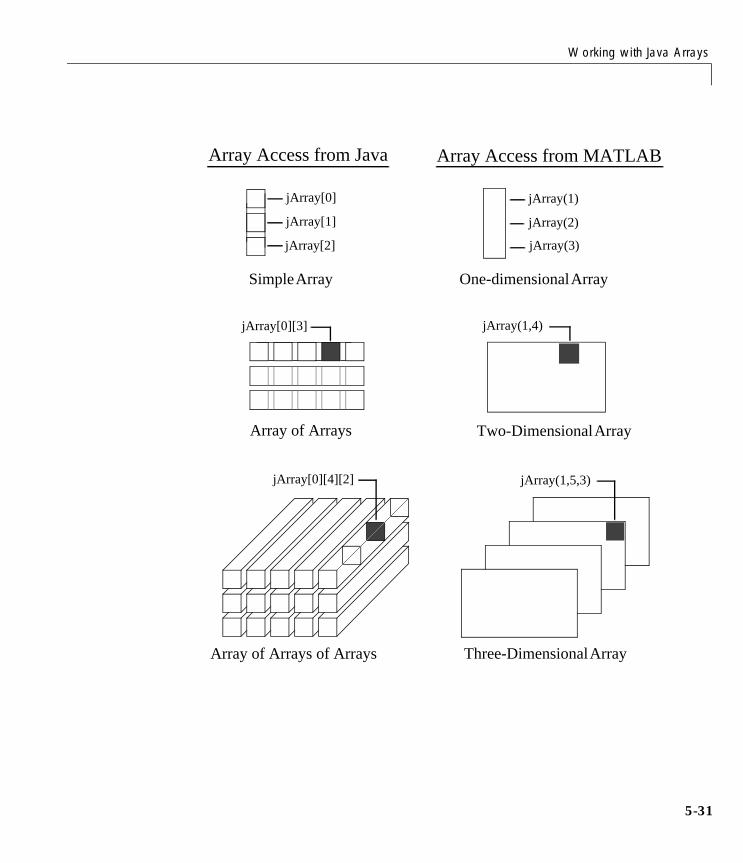
Working with Java Arrays
5-31
Array Access from Java Array Access from MATLAB
jArray[0][4][2] jArray(1,5,3)
jArray[0][3] jArray(1,4)
jArray[0]
jArray[1]
jArray[2]
jArray(1)
jArray(2)
jArray(3)
Array of Arrays Two-Dimensional Array
Simple Array One-dimensional Array
Array of Arrays of Arrays Three-Dimensional Array

5 Calling Java from MATLAB
5-32
Array IndexingJava array indexing is different than MATLAB array indexing. Java array indices are zero-based, MATLAB array indices are one-based. In Java programming, you access the elements of array y of length N using y[0] through y[N-1]. When working with this array in MATLAB, you access these same elements using the MATLAB indexing style of y(1) through y(N). Thus, if you have a Java array of 10 elements, the seventh element is obtained using y(7), and not y[6] as you would have used when writing a program in Java.
The Shape of the Java ArrayA Java array can be different from a MATLAB array in its overall shape. A two-dimensional MATLAB array maintains a rectangular shape, as each row is of equal length and each column of equal height. The Java counterpart of this, an array of arrays, does not necessarily hold to this rectangular form. Each individual lower level array may have a different length.
Such an array structure is pictured below. This is an array of three underlying arrays of different lengths. The term ragged is commonly used to describe this arrangement of array elements as the array ends do not match up evenly. When a Java method returns an array with this type of structure, it is stored in a cell array by MATLAB.
Interpreting the Size of a Java ArrayWhen the MATLAB size function is applied to a simple Java array, the number of rows returned is the length of the Java array and the number of columns is always 1.
Determining the size of a Java array of arrays is not so simple. The potentially ragged shape of an array returned from Java makes it impossible to size the array in the same way as for a rectangular matrix. In a ragged Java array, there is no one value that represents the size of the lower level arrays.
jArray[0] length = 5
jArray[1]
jArray[2]
length = 2
length = 3
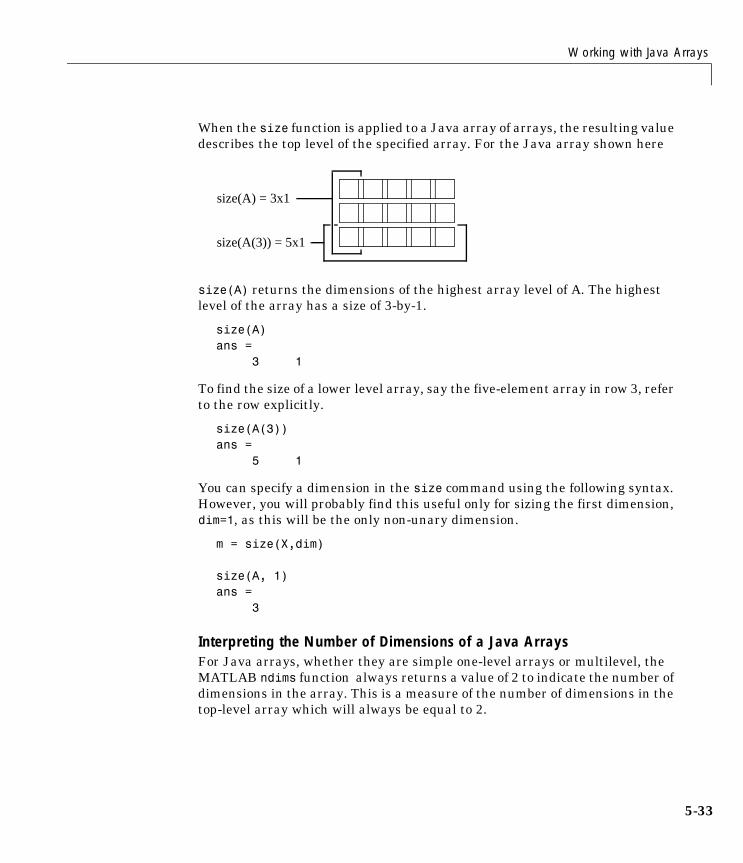
Working with Java Arrays
5-33
When the size function is applied to a Java array of arrays, the resulting value describes the top level of the specified array. For the Java array shown here
size(A) returns the dimensions of the highest array level of A. The highest level of the array has a size of 3-by-1.
size(A)ans = 3 1
To find the size of a lower level array, say the five-element array in row 3, refer to the row explicitly.
size(A(3))ans = 5 1
You can specify a dimension in the size command using the following syntax. However, you will probably find this useful only for sizing the first dimension, dim=1, as this will be the only non-unary dimension.
m = size(X,dim)
size(A, 1)ans = 3
Interpreting the Number of Dimensions of a Java ArraysFor Java arrays, whether they are simple one-level arrays or multilevel, the MATLAB ndims function always returns a value of 2 to indicate the number of dimensions in the array. This is a measure of the number of dimensions in the top-level array which will always be equal to 2.
size(A) = 3x1
size(A(3)) = 5x1
5 Calling Java from MATLAB
5-34
Creating an Array of Objects Within MATLABTo call a Java method that has one or more arguments defined as an array of Java objects, you must, under most circumstances, pass your objects in a Java array. You can construct an array of objects in a call to a Java method or constructor. Or you can create the array within MATLAB.
The MATLAB javaArray function lets you create a Java array structure that can be handled in MATLAB as a single multidimensional array. You specify the number and size of the array dimensions along with the class of objects you intend to store in it. Using the one-dimensional Java array as its primary building block, MATLAB then builds an array structure that satisfies the dimensions requested in the javaArray command.
Using the javaArray FunctionTo create a Java object array, use the MATLAB javaArray function, which has the following syntax.
A = javaArray('element_class', m, n, p, ...)
The first argument is the ’element_class’ string, which names the class of the elements in the array. You must specify the fully qualified name (package and class name). The remaining arguments (m, n, p, ...) are the number of elements in each dimension of the array.
An array that you create with javaArray is equivalent to the array that you would create with the Java code.
A = new element_class[m][n][p]...;
The following command builds a Java array of four lower level arrays, each capable of holding five objects of the java.lang.Double class. (You will probably be more likely to use primitive types of double than instances of the java.lang.Double class, but in this context, it affords us a simple example.)
dblArray = javaArray('java.lang.Double', 4, 5);
The javaArray function does not deposit any values into the array elements that it creates. You must do this separately. The following MATLAB code stores objects of the java.lang.Double type in the Java array dblArray that was just created.
Working with Java Arrays
5-35
for m = 1:4 for n = 1:5 dblArray(m,n) = java.lang.Double((m*10) + n); endend
dblArraydblArray =java.lang.Double[][]: [11] [12] [13] [14] [15] [21] [22] [23] [24] [25] [31] [32] [33] [34] [35] [41] [42] [43] [44] [45]
Another Way to Create a Java ArrayYou can also create an array of Java objects using syntax that is more typical to MATLAB. For example, the following syntax creates a 4-by-5 MATLAB array of type double and assigns zero to each element of the array.
matlabArray(4,5) = 0;
You use similar syntax to create a Java array in MATLAB, except that you must specify the Java class name. The value being assigned, 0 in this example, is stored in the final element of the array, javaArray(4,5). All other elements of the array receive the empty matrix.
javaArray(4,5) = java.lang.Double(0)javaArray =java.lang.Double[][]: [] [] [] [] [] [] [] [] [] [] [] [] [] [] [] [] [] [] [] [0]
Note You cannot change the dimensions of an existing Java array as you can with a MATLAB array. The same restriction exists when working with Java arrays in the Java language. See the example below.
5 Calling Java from MATLAB
5-36
This example first creates a scalar MATLAB array, and then successfully modifies it to be two-dimensional.
matlabArray = 0;matlabArray(4,5) = 0
matlabArray =
0 0 0 0 0 0 0 0 0 0 0 0 0 0 0 0 0 0 0 0
When you try this with a Java array, you get an error. Similarly, you cannot create an array of Java arrays from a Java array, and so forth.
javaArray = java.lang.Double(0);javaArray(4,5) = java.lang.Double(0);??? Index exceeds Java array dimensions.
Accessing Elements of a Java ArrayYou can access elements of a Java object array by using the MATLAB array indexing syntax, A(row,col). For example, to access the element of array dblArray located at row 3, column 4, use
row3_col4 = dblArray(3,4)row3_col4 = 34.0
In Java, this would be dblArray[2][3].
You can also use MATLAB array indexing syntax to access an element in an object’s data field. Suppose that myMenuObj is an instance of a window menu class. This user-supplied class has a data field, menuItemArray, which is a Java array of java.awt.menuItem. To get element 3 of this array, use the following command.
currentItem = myMenuObj.menuItemArray(3)
Using Single Subscript Indexing to Access ArraysElements of a MATLAB matrix are most commonly referenced using both row and column subscripts. For example, you use x(3,4) to reference the array
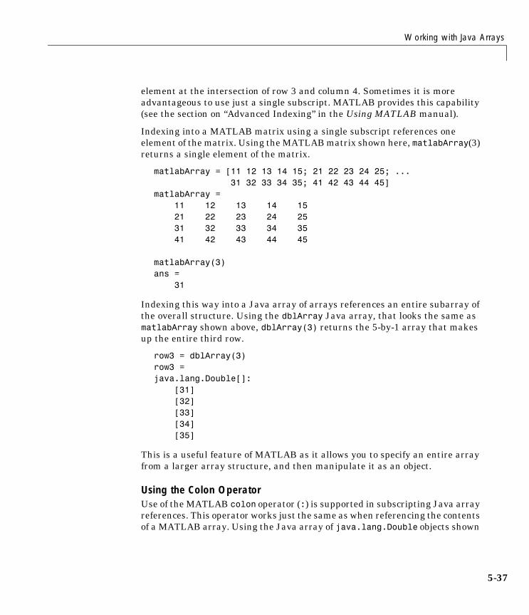
Working with Java Arrays
5-37
element at the intersection of row 3 and column 4. Sometimes it is more advantageous to use just a single subscript. MATLAB provides this capability (see the section on “Advanced Indexing” in the Using MATLAB manual).
Indexing into a MATLAB matrix using a single subscript references one element of the matrix. Using the MATLAB matrix shown here, matlabArray(3) returns a single element of the matrix.
matlabArray = [11 12 13 14 15; 21 22 23 24 25; ... 31 32 33 34 35; 41 42 43 44 45]matlabArray = 11 12 13 14 15 21 22 23 24 25 31 32 33 34 35 41 42 43 44 45
matlabArray(3)ans = 31
Indexing this way into a Java array of arrays references an entire subarray of the overall structure. Using the dblArray Java array, that looks the same as matlabArray shown above, dblArray(3) returns the 5-by-1 array that makes up the entire third row.
row3 = dblArray(3)row3 =java.lang.Double[]: [31] [32] [33] [34] [35]
This is a useful feature of MATLAB as it allows you to specify an entire array from a larger array structure, and then manipulate it as an object.
Using the Colon OperatorUse of the MATLAB colon operator (:) is supported in subscripting Java array references. This operator works just the same as when referencing the contents of a MATLAB array. Using the Java array of java.lang.Double objects shown
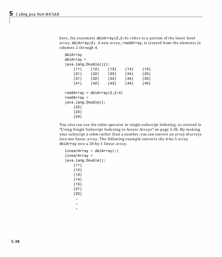
5 Calling Java from MATLAB
5-38
here, the statement dblArray(2,2:4) refers to a portion of the lower level array, dblArray(2). A new array, row2Array, is created from the elements in columns 2 through 4.
dblArraydblArray =java.lang.Double[][]: [11] [12] [13] [14] [15] [21] [22] [23] [24] [25] [31] [32] [33] [34] [35] [41] [42] [43] [44] [45]
row2Array = dblArray(2,2:4)row2Array =java.lang.Double[]: [22] [23] [24]
You also can use the colon operator in single-subscript indexing, as covered in “Using Single Subscript Indexing to Access Arrays” on page 5-36. By making your subscript a colon rather than a number, you can convert an array of arrays into one linear array. The following example converts the 4-by-5 array dblArray into a 20-by-1 linear array.
linearArray = dblArray(:)linearArray = java.lang.Double[]: [11] [12] [13] [14] [15] [21] [22] . . .
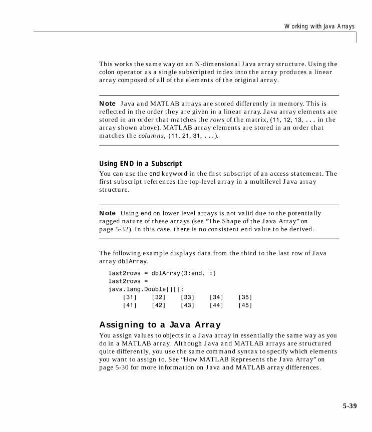
Working with Java Arrays
5-39
This works the same way on an N-dimensional Java array structure. Using the colon operator as a single subscripted index into the array produces a linear array composed of all of the elements of the original array.
Note Java and MATLAB arrays are stored differently in memory. This is reflected in the order they are given in a linear array. Java array elements are stored in an order that matches the rows of the matrix, (11, 12, 13, ... in the array shown above). MATLAB array elements are stored in an order that matches the columns, (11, 21, 31, ...).
Using END in a SubscriptYou can use the end keyword in the first subscript of an access statement. The first subscript references the top-level array in a multilevel Java array structure.
Note Using end on lower level arrays is not valid due to the potentially ragged nature of these arrays (see “The Shape of the Java Array” on page 5-32). In this case, there is no consistent end value to be derived.
The following example displays data from the third to the last row of Java array dblArray.
last2rows = dblArray(3:end, :)last2rows =java.lang.Double[][]: [31] [32] [33] [34] [35] [41] [42] [43] [44] [45]
Assigning to a Java ArrayYou assign values to objects in a Java array in essentially the same way as you do in a MATLAB array. Although Java and MATLAB arrays are structured quite differently, you use the same command syntax to specify which elements you want to assign to. See “How MATLAB Represents the Java Array” on page 5-30 for more information on Java and MATLAB array differences.
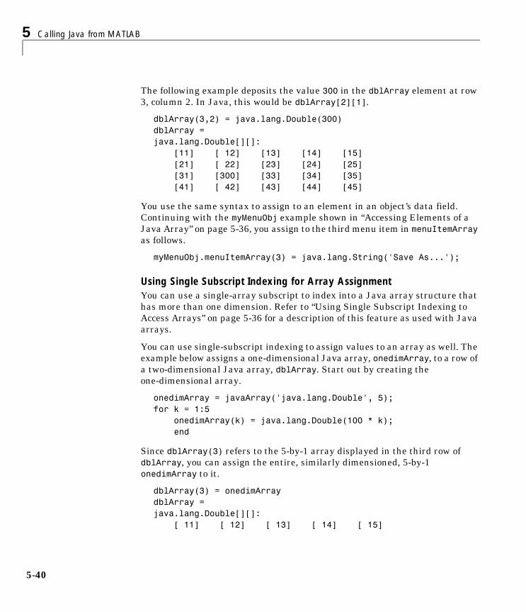
5 Calling Java from MATLAB
5-40
The following example deposits the value 300 in the dblArray element at row 3, column 2. In Java, this would be dblArray[2][1].
dblArray(3,2) = java.lang.Double(300)dblArray =java.lang.Double[][]: [11] [ 12] [13] [14] [15] [21] [ 22] [23] [24] [25] [31] [300] [33] [34] [35] [41] [ 42] [43] [44] [45]
You use the same syntax to assign to an element in an object’s data field. Continuing with the myMenuObj example shown in “Accessing Elements of a Java Array” on page 5-36, you assign to the third menu item in menuItemArray as follows.
myMenuObj.menuItemArray(3) = java.lang.String('Save As...');
Using Single Subscript Indexing for Array AssignmentYou can use a single-array subscript to index into a Java array structure that has more than one dimension. Refer to “Using Single Subscript Indexing to Access Arrays” on page 5-36 for a description of this feature as used with Java arrays.
You can use single-subscript indexing to assign values to an array as well. The example below assigns a one-dimensional Java array, onedimArray, to a row of a two-dimensional Java array, dblArray. Start out by creating the one-dimensional array.
onedimArray = javaArray('java.lang.Double', 5);for k = 1:5 onedimArray(k) = java.lang.Double(100 * k); end
Since dblArray(3) refers to the 5-by-1 array displayed in the third row of dblArray, you can assign the entire, similarly dimensioned, 5-by-1 onedimArray to it.
dblArray(3) = onedimArraydblArray =java.lang.Double[][]: [ 11] [ 12] [ 13] [ 14] [ 15]

Working with Java Arrays
5-41
[ 21] [ 22] [ 23] [ 24] [ 25] [100] [200] [300] [400] [500] [ 41] [ 42] [ 43] [ 44] [ 45]
Assigning to a Linear ArrayYou can assign a value to every element of a multidimensional Java array by treating the array structure as if it were a single linear array. This entails replacing the single, numerical subscript with the MATLAB colon operator. If you start with the dblArray array, you can initialize the contents of every object in the two-dimensional array with the following statement.
dblArray(:) = java.lang.Double(0)dblArray =java.lang.Double[][]: [0] [0] [0] [0] [0] [0] [0] [0] [0] [0] [0] [0] [0] [0] [0] [0] [0] [0] [0] [0]
Using the Colon Operator
You can use the MATLAB colon operator as you would when working with MATLAB arrays. The statements below assign given values to each of the four rows in the Java array, dblArray. Remember that each row actually represents a separate Java array in itself.
dblArray(1,:) = java.lang.Double(125);dblArray(2,:) = java.lang.Double(250);dblArray(3,:) = java.lang.Double(375);dblArray(4,:) = java.lang.Double(500)dblArray =java.lang.Double[][]: [125] [125] [125] [125] [125] [250] [250] [250] [250] [250] [375] [375] [375] [375] [375] [500] [500] [500] [500] [500]
Assigning the Empty MatrixWhen working with MATLAB arrays, you can assign the empty matrix, (i.e., the 0-by-0 array denoted by []) to an element of the array. For Java arrays, you
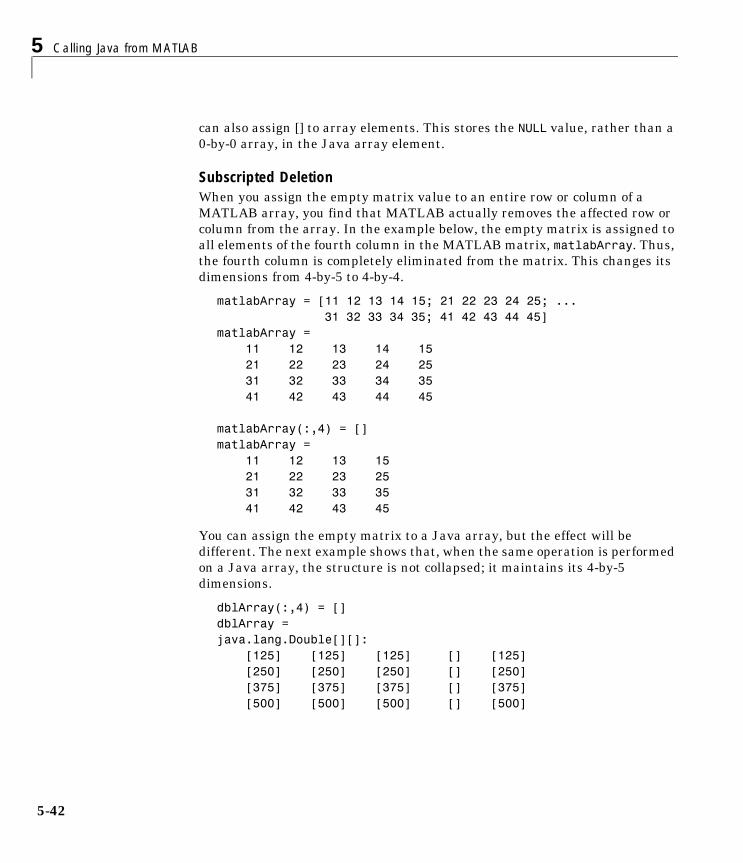
5 Calling Java from MATLAB
5-42
can also assign [] to array elements. This stores the NULL value, rather than a 0-by-0 array, in the Java array element.
Subscripted DeletionWhen you assign the empty matrix value to an entire row or column of a MATLAB array, you find that MATLAB actually removes the affected row or column from the array. In the example below, the empty matrix is assigned to all elements of the fourth column in the MATLAB matrix, matlabArray. Thus, the fourth column is completely eliminated from the matrix. This changes its dimensions from 4-by-5 to 4-by-4.
matlabArray = [11 12 13 14 15; 21 22 23 24 25; ... 31 32 33 34 35; 41 42 43 44 45]matlabArray = 11 12 13 14 15 21 22 23 24 25 31 32 33 34 35 41 42 43 44 45
matlabArray(:,4) = []matlabArray = 11 12 13 15 21 22 23 25 31 32 33 35 41 42 43 45
You can assign the empty matrix to a Java array, but the effect will be different. The next example shows that, when the same operation is performed on a Java array, the structure is not collapsed; it maintains its 4-by-5 dimensions.
dblArray(:,4) = []dblArray =java.lang.Double[][]: [125] [125] [125] [] [125] [250] [250] [250] [] [250] [375] [375] [375] [] [375] [500] [500] [500] [] [500]
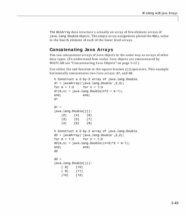
Working with Java Arrays
5-43
The dblArray data structure s actually an array of five-element arrays of java.lang.Double objects. The empty array assignment placed the NULL value in the fourth element of each of the lower level arrays.
Concatenating Java ArraysYou can concatenate arrays of Java objects in the same way as arrays of other data types. (To understand how scalar Java objects are concatenated by MATLAB see “Concatenating Java Objects” on page 5-12.)
Use either the cat function or the square bracket ([]) operators. This example horizontally concatenates two Java arrays: d1, and d2.
% Construct a 2-by-3 array of java.lang.Double.d1 = javaArray('java.lang.Double',2,3);for m = 1:3 for n = 1:3d1(m,n) = java.lang.Double(n*2 + m-1);end; end;d1
d1 =java.lang.Double[][]: [2] [4] [6] [3] [5] [7] [4] [6] [8]
% Construct a 2-by-2 array of java.lang.Double.d2 = javaArray('java.lang.Double',2,2);for m = 1:3 for n = 1:2d2(m,n) = java.lang.Double((n+3)*2 + m-1);end; end;d2
d2 =java.lang.Double[][]: [ 8] [10] [ 9] [11] [10] [12]

5 Calling Java from MATLAB
5-44
% Concatenate the two along the second dimension.d3 = cat(2,d1,d2)
d3 =java.lang.Double[][]: [2] [4] [6] [ 8] [10] [3] [5] [7] [ 9] [11] [4] [6] [8] [10] [12]
Creating a New Array ReferenceBecause Java arrays in MATLAB are references, assigning an array variable to another variable results in a second reference to the array.
Consider the following example where two separate array variables reference a common array. The original array, origArray, is created and initialized. The statement newArrayRef = origArray creates a copy of this array variable. Changes made to the array referred to by newArrayRef also show up in the original array.
origArray = javaArray('java.lang.Double', 3, 4);for m = 1:3 for n = 1:4 origArray(m,n) = java.lang.Double((m * 10) + n); endend
origArrayorigArray =java.lang.Double[][]: [11] [12] [13] [14] [21] [22] [23] [24] [31] [32] [33] [34]
% ----- Make a copy of the array reference -----newArrayRef = origArray;newArrayRef(3,:) = java.lang.Double(0);
origArrayorigArray =
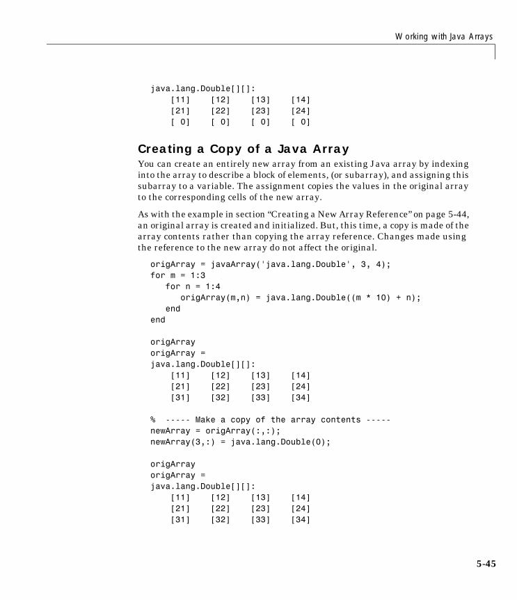
Working with Java Arrays
5-45
java.lang.Double[][]: [11] [12] [13] [14] [21] [22] [23] [24] [ 0] [ 0] [ 0] [ 0]
Creating a Copy of a Java ArrayYou can create an entirely new array from an existing Java array by indexing into the array to describe a block of elements, (or subarray), and assigning this subarray to a variable. The assignment copies the values in the original array to the corresponding cells of the new array.
As with the example in section “Creating a New Array Reference” on page 5-44, an original array is created and initialized. But, this time, a copy is made of the array contents rather than copying the array reference. Changes made using the reference to the new array do not affect the original.
origArray = javaArray('java.lang.Double', 3, 4);for m = 1:3 for n = 1:4 origArray(m,n) = java.lang.Double((m * 10) + n); endend
origArrayorigArray =java.lang.Double[][]: [11] [12] [13] [14] [21] [22] [23] [24] [31] [32] [33] [34]
% ----- Make a copy of the array contents -----newArray = origArray(:,:);newArray(3,:) = java.lang.Double(0);
origArrayorigArray = java.lang.Double[][]: [11] [12] [13] [14] [21] [22] [23] [24] [31] [32] [33] [34]
5 Calling Java from MATLAB
5-46
Passing Data to a Java MethodWhen you make a call from MATLAB to Java code, any MATLAB data types you pass in the call are converted to data types native to the Java language. MATLAB performs this conversion on each argument that is passed, except for those arguments that are already Java objects. This section describes the conversion that is performed on specific MATLAB data types and, at the end, also takes a look at how argument types affect calls made to overloaded methods.
If data is to be returned by the method being called, MATLAB receives this data and converts it to the appropriate MATLAB format wherever necessary. This process is covered in the next section entitled “Handling Data Returned from a Java Method” on page 5-56.
This section addresses the following topics:
• “Conversion of MATLAB Argument Data”
• “Passing Built-In Data Types”
• “Passing String Arguments”
• “Passing Java Objects”
• “Other Data Conversion Topics”
• “Passing Data to Overloaded Methods”
Conversion of MATLAB Argument DataMATLAB data, passed as arguments to Java methods, are converted by MATLAB into data types that best represent the data to the Java language. The table below shows all of the MATLAB base types for passed arguments and the Java base types defined for input arguments. Each row shows a MATLAB type followed by the possible Java argument matches, from left to right in order of closeness of the match. The MATLAB types (except cell arrays) can all be
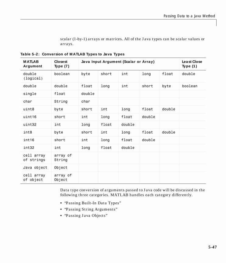
Passing Data to a Java Method
5-47
scalar (1-by-1) arrays or matrices. All of the Java types can be scalar values or arrays.
Data type conversion of arguments passed to Java code will be discussed in the following three categories. MATLAB handles each category differently.
• “Passing Built-In Data Types”
• “Passing String Arguments”
• “Passing Java Objects”
Table 5-2: Conversion of MATLAB Types to Java Types
MATLAB Argument
Closest Type (7)
Java Input Argument (Scalar or Array) Least Close Type (1)
double (logical)
boolean byte short int long float double
double double float long int short byte boolean
single float double
char String char
uint8 byte short int long float double
uint16 short int long float double
uint32 int long float double
int8 byte short int long float double
int16 short int long float double
int32 int long float double
cell array of strings
array of String
Java object Object
cell array of object
array of Object
5 Calling Java from MATLAB
5-48
Passing Built-In Data TypesJava has eight data types that are intrinsic to the language and are not represented as Java objects. These are often referred to as built-in, or elemental, data types and they include boolean, byte, short, long, int, double, float, and char. MATLAB converts its own data types to these Java built-in types according to the table, “Conversion of MATLAB Types to Java Types” on page 5-47. Built-in types are in the first 10 rows of the table.
When a Java method you are calling expects one of these data types, you can pass it the type of MATLAB argument shown in the left-most column of the table. If the method takes an array of one of these types, you can pass a MATLAB array of the data type. MATLAB converts the data type of the argument to the type assigned in the method declaration.
The MATLAB code shown below creates a top-level window frame and sets its dimensions. The call to setBounds passes four MATLAB scalars of the double type to the inherited Java Frame method, setBounds, that takes four arguments of the int type. MATLAB converts each 64-bit double data type to a 32-bit integer prior to making the call. Shown here is the setBounds method declaration followed by the MATLAB code that calls the method.
public void setBounds(int x, int y, int width, int height)
frame=java.awt.Frame;frame.setBounds(200,200,800,400);frame.setVisible(1);
Passing Built-In Types in an ArrayTo call a Java method with an argument defined as an array of a built-in type, you can create and pass a MATLAB matrix with a compatible base type. The following code defines a polygon by sending four x and y coordinates to the Polygon constructor. Two 1-by-4 MATLAB arrays of double are passed to java.awt.Polygon, which expects integer arrays in the first two arguments. Shown here is the Java method declaration followed by MATLAB code that calls the method, and then verifies the set coordinates.
public Polygon(int xpoints[], int ypoints[], int npoints)
poly = java.awt.Polygon([14 42 98 124], [55 12 -2 62], 4);
Passing Data to a Java Method
5-49
[poly.xpoints poly.ypoints] % Verify the coordinatesans =14 5542 1298 -2124 62
MATLAB Arrays Are Passed by ValueSince MATLAB arrays are passed by value, any changes that a Java method makes to them will not be visible to your MATLAB code. If you need to access changes that a Java method makes to an array, then, rather than passing a MATLAB array, you should create and pass a Java array, which is a reference. For a description of using Java arrays in MATLAB, see “Working with Java Arrays” on page 5-29.
Note Generally, it is preferable to have methods return data that has been modified using the return argument mechanism as opposed to passing a reference to that data in an argument list.
Passing String ArgumentsTo call a Java method that has an argument defined as an object of class java.lang.String, you can pass either a String object that was returned from an earlier Java call or a MATLAB 1-by-n character array. If you pass the character array, MATLAB converts the array to a Java object of java.lang.String for you.
For a programming example, see “Example – Reading a URL” on page 5-63. This shows a MATLAB character array that holds a URL being passed to the Java URL class constructor. The constructor, shown below, expects a Java String argument.
public URL(String spec) throws MalformedURLException
5 Calling Java from MATLAB
5-50
In the MATLAB call to this constructor, a character array specifying the URL is passed. MATLAB converts this array to a Java String object prior to calling the constructor.
url = java.net.URL(... 'http://www.ncsa.uiuc.edu/demoweb/url-primer.html')
Passing Strings in an ArrayWhen the method you are calling expects an argument of an array of type String, you can create such an array by packaging the strings together in a MATLAB cell array. The strings can be of varying lengths since you are storing them in different cells of the array. As part of the method call, MATLAB converts the cell array to a Java array of String objects.
In the following example, the echoPrompts method of a user-written class accepts a string array argument that MATLAB converted from its original format as a cell array of strings. The parameter list in the Java method appears as follows.
public String[] echoPrompts(String s[])
You create the input argument by storing both strings in a MATLAB cell array. MATLAB converts this structure to a Java array of String.
myaccount.echoPrompts({'Username: ','Password: '})ans = 'Username: ''Password: '
Passing Java ObjectsWhen calling a method that has an argument belonging to a particular Java class, you must pass an object that is an instance of that class. In the example below, the add method belonging to the java.awt.Menu class requires, as an argument, an object of the java.awt.MenuItem class. The method declaration for this is
public MenuItem add(MenuItem mi)
The example operates on the frame created in the previous example in “Passing Built-In Data Types” on page 5-48. The second, third, and fourth lines of code shown here add items to a menu to be attached to the existing window frame.
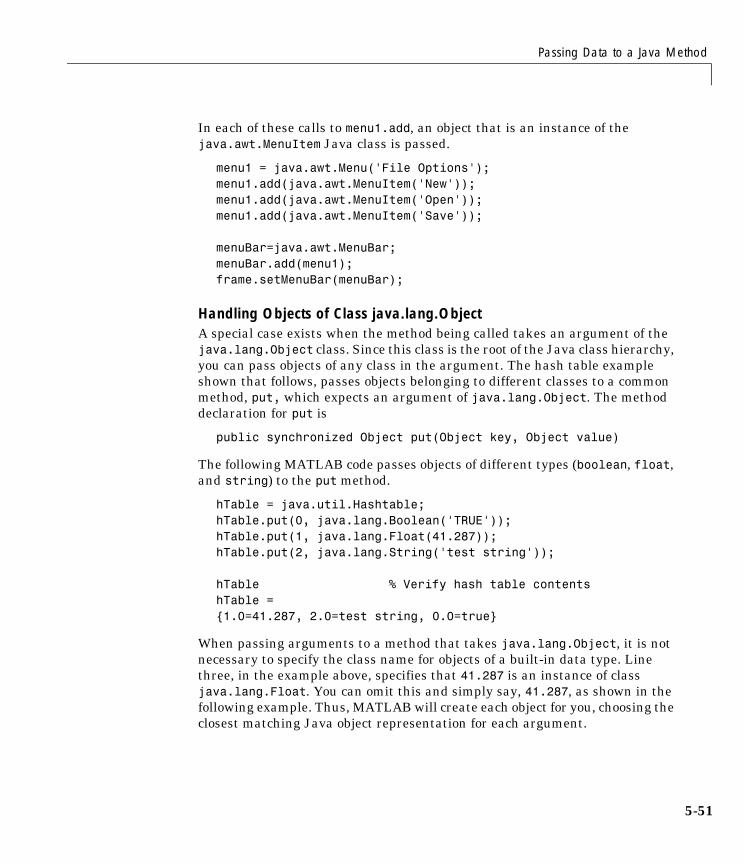
Passing Data to a Java Method
5-51
In each of these calls to menu1.add, an object that is an instance of the java.awt.MenuItem Java class is passed.
menu1 = java.awt.Menu('File Options');menu1.add(java.awt.MenuItem('New'));menu1.add(java.awt.MenuItem('Open'));menu1.add(java.awt.MenuItem('Save'));
menuBar=java.awt.MenuBar;menuBar.add(menu1);frame.setMenuBar(menuBar);
Handling Objects of Class java.lang.ObjectA special case exists when the method being called takes an argument of the java.lang.Object class. Since this class is the root of the Java class hierarchy, you can pass objects of any class in the argument. The hash table example shown that follows, passes objects belonging to different classes to a common method, put, which expects an argument of java.lang.Object. The method declaration for put is
public synchronized Object put(Object key, Object value)
The following MATLAB code passes objects of different types (boolean, float, and string) to the put method.
hTable = java.util.Hashtable;hTable.put(0, java.lang.Boolean('TRUE'));hTable.put(1, java.lang.Float(41.287));hTable.put(2, java.lang.String('test string'));
hTable % Verify hash table contentshTable ={1.0=41.287, 2.0=test string, 0.0=true}
When passing arguments to a method that takes java.lang.Object, it is not necessary to specify the class name for objects of a built-in data type. Line three, in the example above, specifies that 41.287 is an instance of class java.lang.Float. You can omit this and simply say, 41.287, as shown in the following example. Thus, MATLAB will create each object for you, choosing the closest matching Java object representation for each argument.
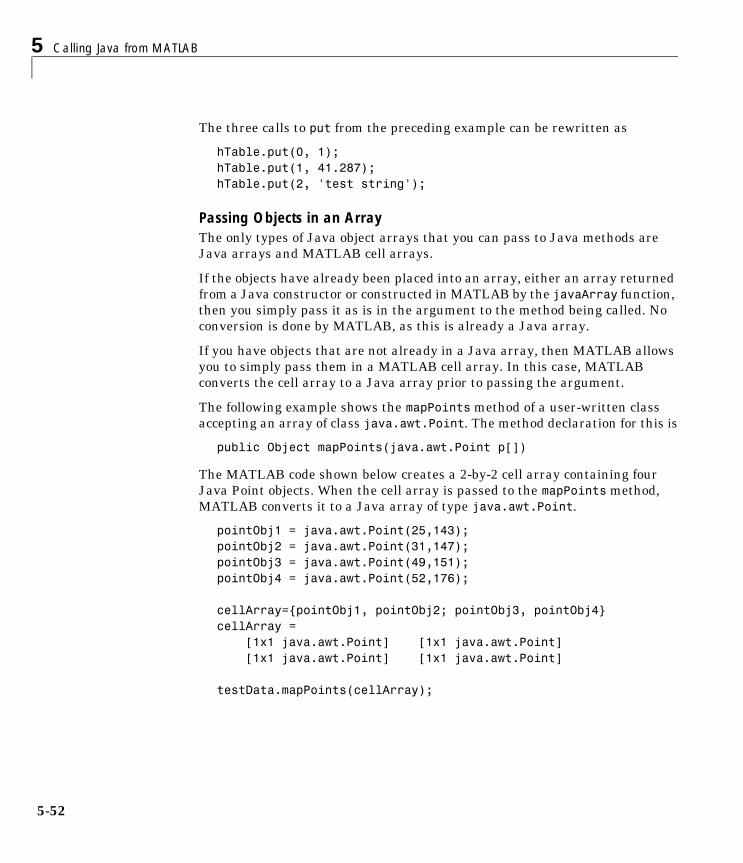
5 Calling Java from MATLAB
5-52
The three calls to put from the preceding example can be rewritten as
hTable.put(0, 1);hTable.put(1, 41.287);hTable.put(2, 'test string');
Passing Objects in an ArrayThe only types of Java object arrays that you can pass to Java methods are Java arrays and MATLAB cell arrays.
If the objects have already been placed into an array, either an array returned from a Java constructor or constructed in MATLAB by the javaArray function, then you simply pass it as is in the argument to the method being called. No conversion is done by MATLAB, as this is already a Java array.
If you have objects that are not already in a Java array, then MATLAB allows you to simply pass them in a MATLAB cell array. In this case, MATLAB converts the cell array to a Java array prior to passing the argument.
The following example shows the mapPoints method of a user-written class accepting an array of class java.awt.Point. The method declaration for this is
public Object mapPoints(java.awt.Point p[])
The MATLAB code shown below creates a 2-by-2 cell array containing four Java Point objects. When the cell array is passed to the mapPoints method, MATLAB converts it to a Java array of type java.awt.Point.
pointObj1 = java.awt.Point(25,143);pointObj2 = java.awt.Point(31,147);pointObj3 = java.awt.Point(49,151);pointObj4 = java.awt.Point(52,176);
cellArray={pointObj1, pointObj2; pointObj3, pointObj4}cellArray = [1x1 java.awt.Point] [1x1 java.awt.Point] [1x1 java.awt.Point] [1x1 java.awt.Point]
testData.mapPoints(cellArray);
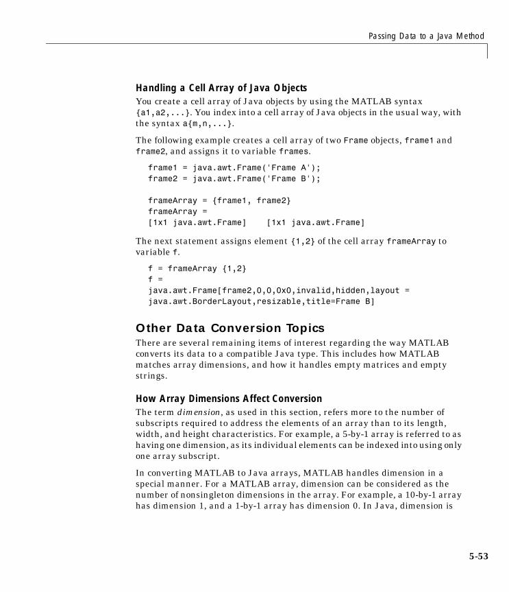
Passing Data to a Java Method
5-53
Handling a Cell Array of Java ObjectsYou create a cell array of Java objects by using the MATLAB syntax {a1,a2,...}. You index into a cell array of Java objects in the usual way, with the syntax a{m,n,...}.
The following example creates a cell array of two Frame objects, frame1 and frame2, and assigns it to variable frames.
frame1 = java.awt.Frame('Frame A');frame2 = java.awt.Frame('Frame B');
frameArray = {frame1, frame2}frameArray = [1x1 java.awt.Frame] [1x1 java.awt.Frame]
The next statement assigns element {1,2} of the cell array frameArray to variable f.
f = frameArray {1,2}f =java.awt.Frame[frame2,0,0,0x0,invalid,hidden,layout = java.awt.BorderLayout,resizable,title=Frame B]
Other Data Conversion TopicsThere are several remaining items of interest regarding the way MATLAB converts its data to a compatible Java type. This includes how MATLAB matches array dimensions, and how it handles empty matrices and empty strings.
How Array Dimensions Affect ConversionThe term dimension, as used in this section, refers more to the number of subscripts required to address the elements of an array than to its length, width, and height characteristics. For example, a 5-by-1 array is referred to as having one dimension, as its individual elements can be indexed into using only one array subscript.
In converting MATLAB to Java arrays, MATLAB handles dimension in a special manner. For a MATLAB array, dimension can be considered as the number of nonsingleton dimensions in the array. For example, a 10-by-1 array has dimension 1, and a 1-by-1 array has dimension 0. In Java, dimension is
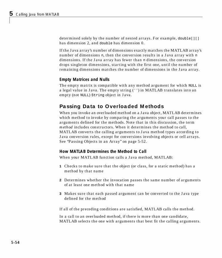
5 Calling Java from MATLAB
5-54
determined solely by the number of nested arrays. For example, double[][] has dimension 2, and double has dimension 0.
If the Java array’s number of dimensions exactly matches the MATLAB array’s number of dimensions n, then the conversion results in a Java array with n dimensions. If the Java array has fewer than n dimensions, the conversion drops singleton dimensions, starting with the first one, until the number of remaining dimensions matches the number of dimensions in the Java array.
Empty Matrices and NullsThe empty matrix is compatible with any method argument for which NULL is a legal value in Java. The empty string ('') in MATLAB translates into an empty (not NULL) String object in Java.
Passing Data to Overloaded MethodsWhen you invoke an overloaded method on a Java object, MATLAB determines which method to invoke by comparing the arguments your call passes to the arguments defined for the methods. Note that in this discussion, the term method includes constructors. When it determines the method to call, MATLAB converts the calling arguments to Java method types according to Java conversion rules, except for conversions involving objects or cell arrays. See “Passing Objects in an Array” on page 5-52.
How MATLAB Determines the Method to CallWhen your MATLAB function calls a Java method, MATLAB:
1 Checks to make sure that the object (or class, for a static method) has a method by that name
2 Determines whether the invocation passes the same number of arguments of at least one method with that name
3 Makes sure that each passed argument can be converted to the Java type defined for the method
If all of the preceding conditions are satisfied, MATLAB calls the method.
In a call to an overloaded method, if there is more than one candidate, MATLAB selects the one with arguments that best fit the calling arguments.
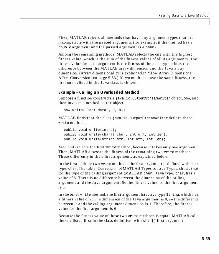
Passing Data to a Java Method
5-55
First, MATLAB rejects all methods that have any argument types that are incompatible with the passed arguments (for example, if the method has a double argument and the passed argument is a char).
Among the remaining methods, MATLAB selects the one with the highest fitness value, which is the sum of the fitness values of all its arguments. The fitness value for each argument is the fitness of the base type minus the difference between the MATLAB array dimension and the Java array dimension. (Array dimensionality is explained in “How Array Dimensions Affect Conversion” on page 5-53.) If two methods have the same fitness, the first one defined in the Java class is chosen.
Example - Calling an Overloaded MethodSuppose a function constructs a java.io.OutputStreamWriter object, osw, and then invokes a method on the object.
osw.write('Test data', 0, 9);
MATLAB finds that the class java.io.OutputStreamWriter defines three write methods.
public void write(int c);public void write(char[] cbuf, int off, int len);public void write(String str, int off, int len);
MATLAB rejects the first write method, because it takes only one argument. Then, MATLAB assesses the fitness of the remaining two write methods. These differ only in their first argument, as explained below.
In the first of these two write methods, the first argument is defined with base type, char. The table, Conversion of MATLAB Types to Java Types, shows that for the type of the calling argument (MATLAB char), Java type, char, has a value of 6. There is no difference between the dimension of the calling argument and the Java argument. So the fitness value for the first argument is 6.
In the other write method, the first argument has Java type String, which has a fitness value of 7. The dimension of the Java argument is 0, so the difference between it and the calling argument dimension is 1. Therefore, the fitness value for the first argument is 6.
Because the fitness value of those two write methods is equal, MATLAB calls the one listed first in the class definition, with char[] first argument.

5 Calling Java from MATLAB
5-56
Handling Data Returned from a Java MethodIn many cases, data returned from Java is incompatible with the data types operated on within MATLAB. When this is the case, MATLAB converts the returned value to a data type native to the MATLAB language. This section describes the conversion performed on the various data types that can be returned from a call to a Java method.
This section addresses the following topics:
• “Conversion of Java Return Data”
• “Built-In Data Types”
• “Java Objects”
• “Converting Objects to MATLAB Data Types”
Conversion of Java Return DataThe following table lists Java return types and the resulting MATLAB types. For some Java base return types, MATLAB treats scalar and array returns differently, as described following the table.
Table 5-3: Conversion of Java Types to MATLAB Types
Java Return Type If Scalar Return, Resulting MATLAB Type
If Array Return, Resulting MATLAB Type
boolean double (logical) double (logical)
byte double int8
short double int16
int double int32
long double double
float double single
double double double
char char char
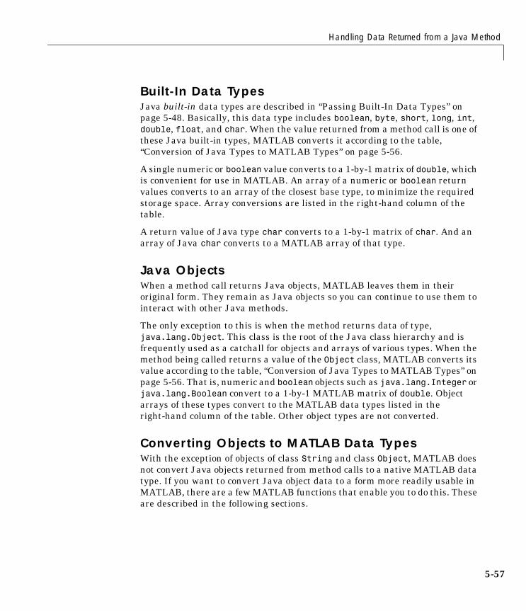
Handling Data Returned from a Java Method
5-57
Built-In Data TypesJava built-in data types are described in “Passing Built-In Data Types” on page 5-48. Basically, this data type includes boolean, byte, short, long, int, double, float, and char. When the value returned from a method call is one of these Java built-in types, MATLAB converts it according to the table, “Conversion of Java Types to MATLAB Types” on page 5-56.
A single numeric or boolean value converts to a 1-by-1 matrix of double, which is convenient for use in MATLAB. An array of a numeric or boolean return values converts to an array of the closest base type, to minimize the required storage space. Array conversions are listed in the right-hand column of the table.
A return value of Java type char converts to a 1-by-1 matrix of char. And an array of Java char converts to a MATLAB array of that type.
Java ObjectsWhen a method call returns Java objects, MATLAB leaves them in their original form. They remain as Java objects so you can continue to use them to interact with other Java methods.
The only exception to this is when the method returns data of type, java.lang.Object. This class is the root of the Java class hierarchy and is frequently used as a catchall for objects and arrays of various types. When the method being called returns a value of the Object class, MATLAB converts its value according to the table, “Conversion of Java Types to MATLAB Types” on page 5-56. That is, numeric and boolean objects such as java.lang.Integer or java.lang.Boolean convert to a 1-by-1 MATLAB matrix of double. Object arrays of these types convert to the MATLAB data types listed in the right-hand column of the table. Other object types are not converted.
Converting Objects to MATLAB Data TypesWith the exception of objects of class String and class Object, MATLAB does not convert Java objects returned from method calls to a native MATLAB data type. If you want to convert Java object data to a form more readily usable in MATLAB, there are a few MATLAB functions that enable you to do this. These are described in the following sections.

5 Calling Java from MATLAB
5-58
Converting to the MATLAB double Data TypeUsing the double function in MATLAB, you can convert any Java object or array of objects to the MATLAB double data type. The action taken by the double function depends on the class of the object you specify:
• If the object is an instance of a numeric class (java.lang.Number or one of the classes that inherit from that class), then MATLAB uses a preset conversion algorithm to convert the object to a MATLAB double.
• If the object is not an instance of a numeric class, MATLAB checks the class definition to see if it implements a method called toDouble. Note that MATLAB uses toDouble to perform its conversion of Java objects to the MATLAB double data type. If such a method is implemented for this class, MATLAB executes it to perform the conversion.
• If you are using a class of your own design, you can write your own toDouble method to perform conversions on objects of that class to a MATLAB double. This enables you to specify your own means of data type conversion for objects belonging to your own classes.
Note If the class of the specified object is not java.lang.Number, does not inherit from that java.lang.Number, and it does not implement a toDouble method, then an attempt to convert the object using the double function results in an error in MATLAB.
The syntax for the double command is as follows, where object is a Java object or Java array of objects.
double(object);
Converting to the MATLAB char Data TypeWith the MATLAB char function, you can convert java.lang.String objects and arrays to MATLAB data types. A single java.lang.String object converts to a MATLAB character array. An array of java.lang.String objects converts to a MATLAB cell array, with each cell holding a character array.
If the object specified in the char command is not an instance of the java.lang.String class, then MATLAB checks its class to see if it implements a method named toChar. If this is the case, then MATLAB executes the toChar
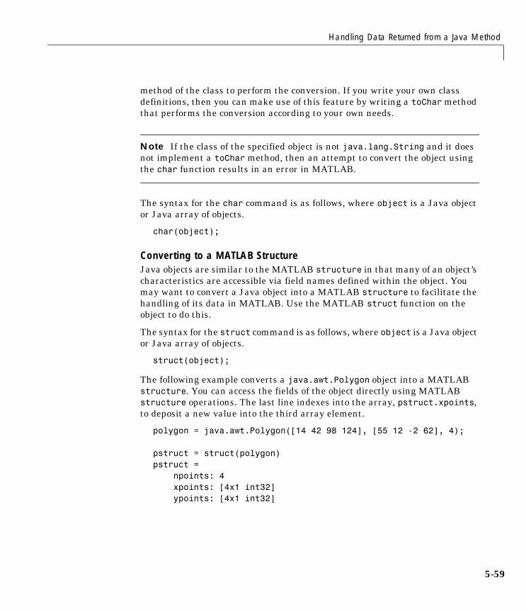
Handling Data Returned from a Java Method
5-59
method of the class to perform the conversion. If you write your own class definitions, then you can make use of this feature by writing a toChar method that performs the conversion according to your own needs.
Note If the class of the specified object is not java.lang.String and it does not implement a toChar method, then an attempt to convert the object using the char function results in an error in MATLAB.
The syntax for the char command is as follows, where object is a Java object or Java array of objects.
char(object);
Converting to a MATLAB StructureJava objects are similar to the MATLAB structure in that many of an object’s characteristics are accessible via field names defined within the object. You may want to convert a Java object into a MATLAB structure to facilitate the handling of its data in MATLAB. Use the MATLAB struct function on the object to do this.
The syntax for the struct command is as follows, where object is a Java object or Java array of objects.
struct(object);
The following example converts a java.awt.Polygon object into a MATLAB structure. You can access the fields of the object directly using MATLAB structure operations. The last line indexes into the array, pstruct.xpoints, to deposit a new value into the third array element.
polygon = java.awt.Polygon([14 42 98 124], [55 12 -2 62], 4);
pstruct = struct(polygon)pstruct = npoints: 4 xpoints: [4x1 int32] ypoints: [4x1 int32]
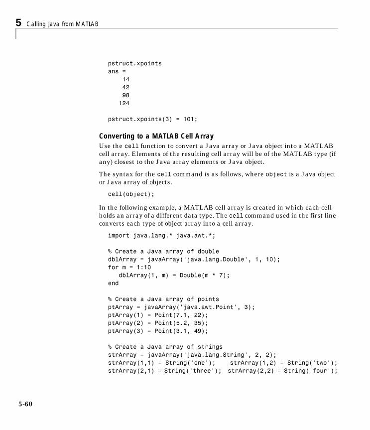
5 Calling Java from MATLAB
5-60
pstruct.xpointsans = 14 42 98 124
pstruct.xpoints(3) = 101;
Converting to a MATLAB Cell ArrayUse the cell function to convert a Java array or Java object into a MATLAB cell array. Elements of the resulting cell array will be of the MATLAB type (if any) closest to the Java array elements or Java object.
The syntax for the cell command is as follows, where object is a Java object or Java array of objects.
cell(object);
In the following example, a MATLAB cell array is created in which each cell holds an array of a different data type. The cell command used in the first line converts each type of object array into a cell array.
import java.lang.* java.awt.*;
% Create a Java array of doubledblArray = javaArray('java.lang.Double', 1, 10);for m = 1:10 dblArray(1, m) = Double(m * 7);end
% Create a Java array of pointsptArray = javaArray('java.awt.Point', 3);ptArray(1) = Point(7.1, 22);ptArray(2) = Point(5.2, 35);ptArray(3) = Point(3.1, 49);
% Create a Java array of stringsstrArray = javaArray('java.lang.String', 2, 2);strArray(1,1) = String('one'); strArray(1,2) = String('two');strArray(2,1) = String('three'); strArray(2,2) = String('four');
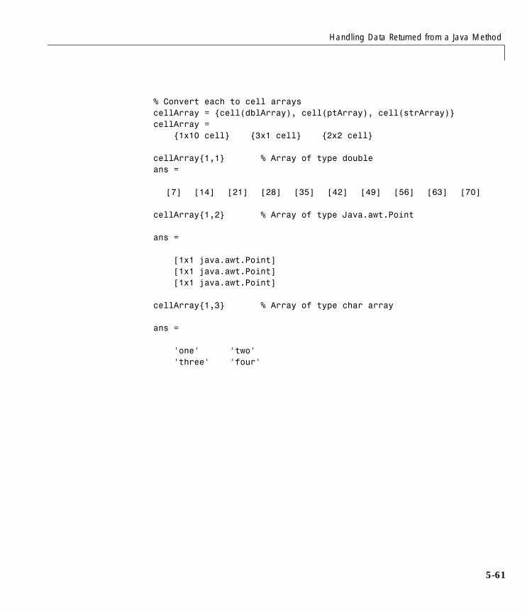
Handling Data Returned from a Java Method
5-61
% Convert each to cell arrayscellArray = {cell(dblArray), cell(ptArray), cell(strArray)}cellArray = {1x10 cell} {3x1 cell} {2x2 cell}
cellArray{1,1} % Array of type doubleans =
[7] [14] [21] [28] [35] [42] [49] [56] [63] [70]
cellArray{1,2} % Array of type Java.awt.Point
ans =
[1x1 java.awt.Point] [1x1 java.awt.Point] [1x1 java.awt.Point]
cellArray{1,3} % Array of type char array
ans =
'one' 'two' 'three' 'four'
5 Calling Java from MATLAB
5-62
Introduction to Programming ExamplesThe following programming examples demonstrate the MATLAB interface to Java classes and objects:
• “Example – Reading a URL”
• “Example – Finding an Internet Protocol Address”
• “Example – Communicating Through a Serial Port”
• “Example – Creating and Using a Phone Book”
Each example contains the following sections:
• Overview - Describes what the example does and how it uses the Java interface to accomplish it. Highlighted are the most important Java objects that are constructed and used in the example code.
• Description - provides a detailed description of all code in the example. For longer functions, the description is divided into functional sections that focus on a few statements.
• Running the Example - Shows a sample of the output from execution of the example code.
The example descriptions concentrate on the Java-related functions. For information on other MATLAB programming constructs, operators, and functions used in the examples, see the applicable sections in the MATLAB documentation.
Example – Reading a URL
5-63
Example – Reading a URLThis program, URLdemo, opens a connection to a web site specified by a URL (Uniform Resource Locator), for the purpose of reading text from a file at that site. It constructs an object of the Java API class, java.net.URL, which enables convenient handling of URLs. Then, it calls a method on the URL object, to open a connection.
To read and display the lines of text at the site, URLdemo uses classes from the Java I/O package java.io. It creates an InputStreamReader object, and then uses that object to construct a BufferedReader object. Finally, it calls a method on the BufferedReader object to read the specified number of lines from the site.
Description of URLdemoThe major tasks performed by URLdemo are:
1. Construct a URL ObjectThe example first calls a constructor on java.net.URL and assigns the resulting object to variable url. The URL constructor takes a single argument, the name of the URL to be accessed, as a string. The constructor checks whether the input URL has a valid form.
url = java.net.URL(... 'http://www.ncsa.uiuc.edu/demoweb/url-primer.html')
2. Open a Connection to the URLThe second statement of the example calls the method, openStream, on the URL object url, to establish a connection with the web site named by the object. The method returns an InputStream object to variable, is, for reading bytes from the site.
is = openStream(url)
3. Set Up a Buffered Stream ReaderThe next two lines create a buffered stream reader for characters. The java.io.InputStreamReader constructor is called with the input stream is, to return to variable isr an object that can read characters. Then, the java.io.BufferedReader constructor is called with isr, to return a
5 Calling Java from MATLAB
5-64
BufferedReader object to variable br. A buffered reader provides for efficient reading of characters, arrays, and lines.
isr = java.io.InputStreamReader(is)br = java.io.BufferedReader(isr)
4. Read and Display Lines of TextThe final statement reads and displays the first 10 lines of text from the site. Within a MATLAB for statement that iterates 10 times, the BufferedReader method readLine reads a line of text (terminated by a return and/or line feed character) from the site. To display the output in MATLAB, assign it to variable s, without terminating the statement with a semicolon.
for k = 1:10s = readLine(br)
end
Running the ExampleWhen you run this example, you see output similar to the following.
url =http://www.ncsa.uiuc.edu/demoweb/url-primer.htmlis =java.io.BufferedInputStream@62disr =java.io.InputStreamReader@67dbr =java.io.BufferedReader@644s =<TITLE>A Beginner's Guide to URLs</TITLE>s =<H1>A Beginner's Guide to URLs</H1>s = ''s =What is a URL? A URL is a <b>Uniform Resource Locator</b>. Think s =of it as a networked extension of the standard <i>filename</i>
Example – Reading a URL
5-65
s =concept: not only can you point to a file in a directory, but that s =file and that directory can exist on any machine on the network, s =can be served via any of several different methods, and might not s =even be something as simple as a file: URLs can also point to s =queries, documents stored deep within databases, the results of a s =<i>finger</i> or <i>archie</i>
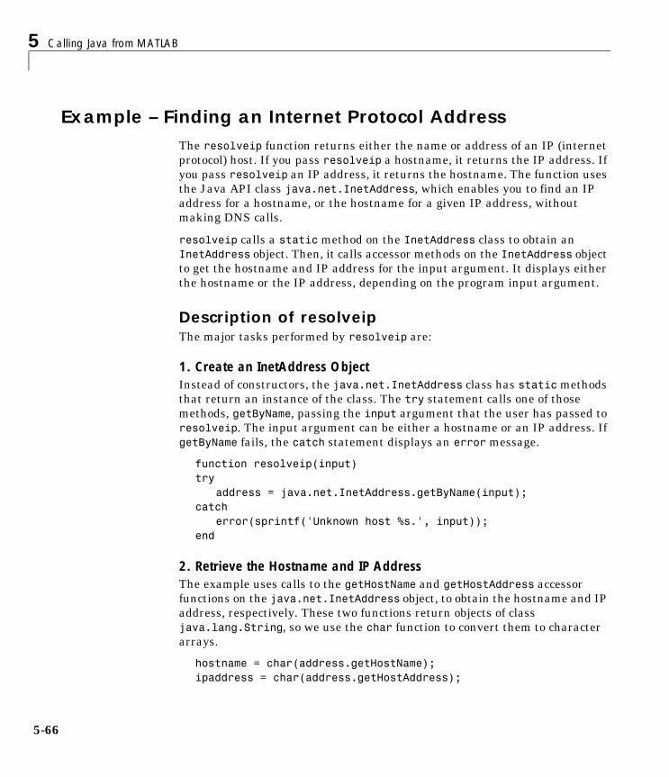
5 Calling Java from MATLAB
5-66
Example – Finding an Internet Protocol AddressThe resolveip function returns either the name or address of an IP (internet protocol) host. If you pass resolveip a hostname, it returns the IP address. If you pass resolveip an IP address, it returns the hostname. The function uses the Java API class java.net.InetAddress, which enables you to find an IP address for a hostname, or the hostname for a given IP address, without making DNS calls.
resolveip calls a static method on the InetAddress class to obtain an InetAddress object. Then, it calls accessor methods on the InetAddress object to get the hostname and IP address for the input argument. It displays either the hostname or the IP address, depending on the program input argument.
Description of resolveipThe major tasks performed by resolveip are:
1. Create an InetAddress ObjectInstead of constructors, the java.net.InetAddress class has static methods that return an instance of the class. The try statement calls one of those methods, getByName, passing the input argument that the user has passed to resolveip. The input argument can be either a hostname or an IP address. If getByName fails, the catch statement displays an error message.
function resolveip(input)try
address = java.net.InetAddress.getByName(input);catch
error(sprintf('Unknown host %s.', input));end
2. Retrieve the Hostname and IP AddressThe example uses calls to the getHostName and getHostAddress accessor functions on the java.net.InetAddress object, to obtain the hostname and IP address, respectively. These two functions return objects of class java.lang.String, so we use the char function to convert them to character arrays.
hostname = char(address.getHostName);ipaddress = char(address.getHostAddress);
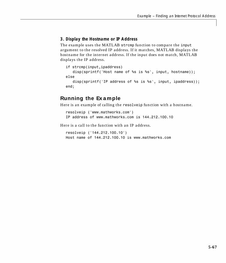
Example – Finding an Internet Protocol Address
5-67
3. Display the Hostname or IP AddressThe example uses the MATLAB strcmp function to compare the input argument to the resolved IP address. If it matches, MATLAB displays the hostname for the internet address. If the input does not match, MATLAB displays the IP address.
if strcmp(input,ipaddress)disp(sprintf('Host name of %s is %s', input, hostname));
else disp(sprintf('IP address of %s is %s', input, ipaddress));
end;
Running the ExampleHere is an example of calling the resolveip function with a hostname.
resolveip ('www.mathworks.com')IP address of www.mathworks.com is 144.212.100.10
Here is a call to the function with an IP address.
resolveip ('144.212.100.10')Host name of 144.212.100.10 is www.mathworks.com
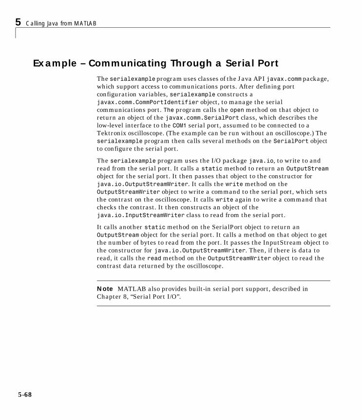
5 Calling Java from MATLAB
5-68
Example – Communicating Through a Serial PortThe serialexample program uses classes of the Java API javax.comm package, which support access to communications ports. After defining port configuration variables, serialexample constructs a javax.comm.CommPortIdentifier object, to manage the serial communications port. The program calls the open method on that object to return an object of the javax.comm.SerialPort class, which describes the low-level interface to the COM1 serial port, assumed to be connected to a Tektronix oscilloscope. (The example can be run without an oscilloscope.) The serialexample program then calls several methods on the SerialPort object to configure the serial port.
The serialexample program uses the I/O package java.io, to write to and read from the serial port. It calls a static method to return an OutputStream object for the serial port. It then passes that object to the constructor for java.io.OutputStreamWriter. It calls the write method on the OutputStreamWriter object to write a command to the serial port, which sets the contrast on the oscilloscope. It calls write again to write a command that checks the contrast. It then constructs an object of the java.io.InputStreamWriter class to read from the serial port.
It calls another static method on the SerialPort object to return an OutputStream object for the serial port. It calls a method on that object to get the number of bytes to read from the port. It passes the InputStream object to the constructor for java.io.OutputStreamWriter. Then, if there is data to read, it calls the read method on the OutputStreamWriter object to read the contrast data returned by the oscilloscope.
Note MATLAB also provides built-in serial port support, described in Chapter 8, “Serial Port I/O”.
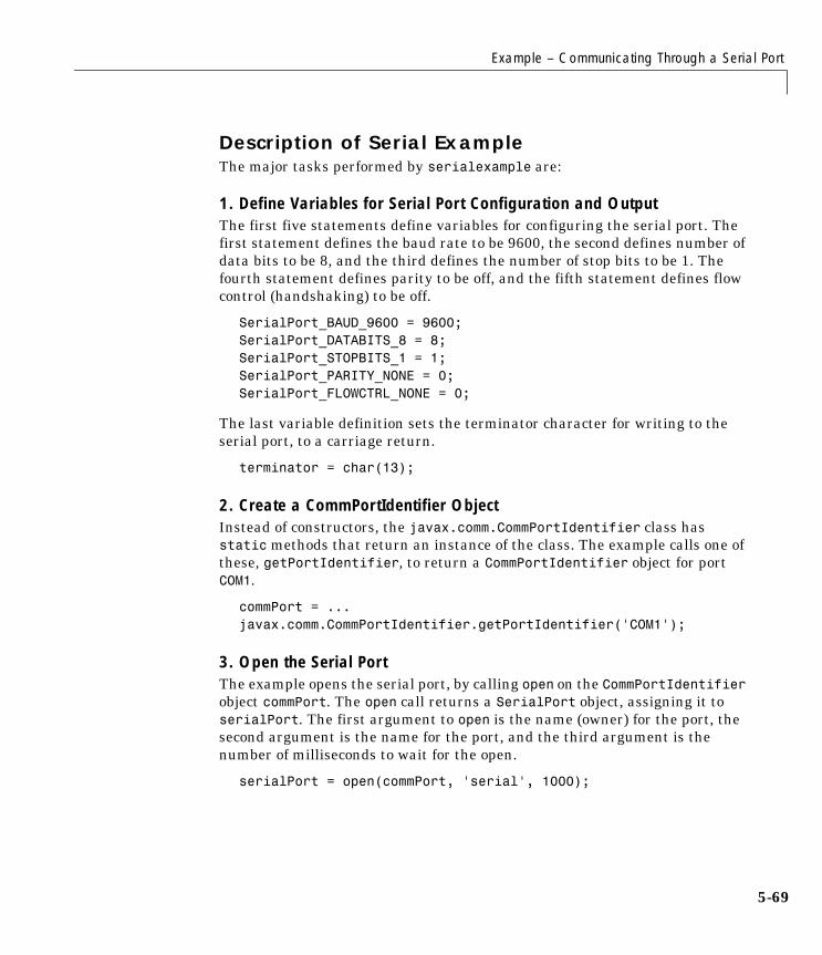
Example – Communicating Through a Serial Port
5-69
Description of Serial ExampleThe major tasks performed by serialexample are:
1. Define Variables for Serial Port Configuration and OutputThe first five statements define variables for configuring the serial port. The first statement defines the baud rate to be 9600, the second defines number of data bits to be 8, and the third defines the number of stop bits to be 1. The fourth statement defines parity to be off, and the fifth statement defines flow control (handshaking) to be off.
SerialPort_BAUD_9600 = 9600;SerialPort_DATABITS_8 = 8;SerialPort_STOPBITS_1 = 1;SerialPort_PARITY_NONE = 0;SerialPort_FLOWCTRL_NONE = 0;
The last variable definition sets the terminator character for writing to the serial port, to a carriage return.
terminator = char(13);
2. Create a CommPortIdentifier ObjectInstead of constructors, the javax.comm.CommPortIdentifier class has static methods that return an instance of the class. The example calls one of these, getPortIdentifier, to return a CommPortIdentifier object for port COM1.
commPort = ... javax.comm.CommPortIdentifier.getPortIdentifier('COM1');
3. Open the Serial PortThe example opens the serial port, by calling open on the CommPortIdentifier object commPort. The open call returns a SerialPort object, assigning it to serialPort. The first argument to open is the name (owner) for the port, the second argument is the name for the port, and the third argument is the number of milliseconds to wait for the open.
serialPort = open(commPort, 'serial', 1000);

5 Calling Java from MATLAB
5-70
4. Configure the Serial PortThe next three statements call configuration methods on the SerialPort object serialPort. The first statement calls setSerialPortParams to set the baud rate, data bits, stop bits, and parity. The next two statements call setFlowControlMode to set the flow control, and then enableReceiveTimeout to set the timeout for receiving data.
setSerialPortParams(serialPort, SerialPort_BAUD_9600,...SerialPort_DATABITS_8, SerialPort_STOPBITS_1,...SerialPort_PARITY_NONE);setFlowControlMode(serialPort, SerialPort_FLOWCTRL_NONE);enableReceiveTimeout(serialPort, 1000);
5. Set Up an Output Stream WriterThe example then calls a constructor to create and open a java.io.OutputStreamWriter object. The constructor call passes the java.io.OutputStream object, returned by a call to the getOutputStream method serialPort, and assigns the OutputStreamWriter object to out.
out = java.io.OutputStreamWriter(getOutputStream(serialPort));
6. Write Data to Serial Port and Close Output StreamThe example writes a string to the serial port, by calling write on the object out. The string is formed by concatenating (with MATLAB [ ] syntax) a command to set the oscilloscope’s contrast to 45, with the command terminator that is required by the instrument. The next statement calls flush on out to flush the output stream.
write(out, ['Display:Contrast 45' terminator]);flush(out);
Then, the example again calls write on out to send another string to the serial port. This string is a query command, to determine the oscilloscope’s contrast setting, concatenated with the command terminator. The example then calls close on the output stream.
write(out, ['Display:Contrast?' terminator]);close(out);

Example – Communicating Through a Serial Port
5-71
7. Open an Input Stream and Determine Number of Bytes to ReadTo read the data expected from the oscilloscope in response to the contrast query, the example opens an input stream by calling the static method, InputStream.getInputStream, to obtain an InputStream object for the serial port. Then, the example calls the method available on the InputStream object, in, and assigns the returned number of bytes to numAvail.
in = getInputStream(serialPort);numAvail = available(in);
8. Create an Input Stream Reader for the Serial PortThe example then calls a java.io.InputStreamReader constructor, with the InputStream object, in, and assigns the new object to reader.
reader = java.io.InputStreamReader(in);
9. Read Data from Serial Port and Close ReaderThe example reads from the serial port, by calling the read method on the InputStreamReader object reader for each available byte. The read statement uses MATLAB array concatenation to add each newly read byte to the array of bytes already read. After reading the data, the example calls close on reader to close the input stream reader.
result = [];for k = 1:numAvail
result = [result read(reader)];endclose(reader);
10. Close the Serial PortThe example closes the serial port, by calling close on the serialPort object.
close(serialPort);
11. Convert Input Argument to a MATLAB Character ArrayThe last statement of the example uses the MATLAB function, char, to convert the array input bytes (integers) to an array of characters:
result = char(result);
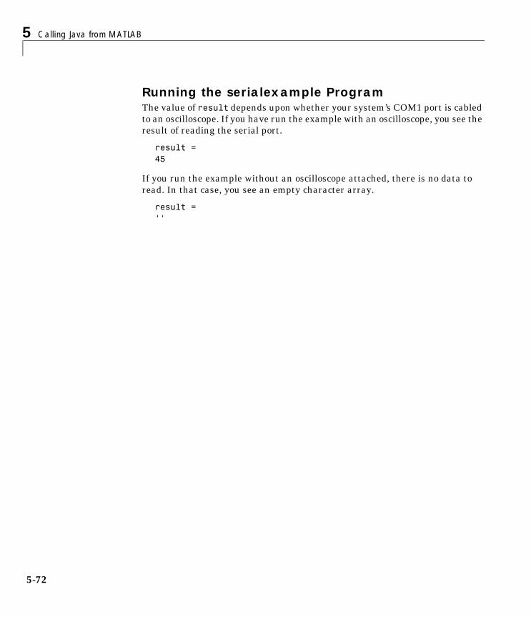
5 Calling Java from MATLAB
5-72
Running the serialexample ProgramThe value of result depends upon whether your system’s COM1 port is cabled to an oscilloscope. If you have run the example with an oscilloscope, you see the result of reading the serial port.
result =45
If you run the example without an oscilloscope attached, there is no data to read. In that case, you see an empty character array.
result =''
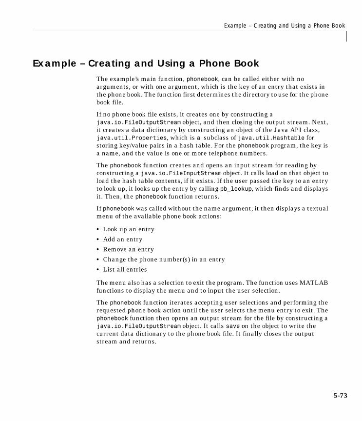
Example – Creating and Using a Phone Book
5-73
Example – Creating and Using a Phone BookThe example’s main function, phonebook, can be called either with no arguments, or with one argument, which is the key of an entry that exists in the phone book. The function first determines the directory to use for the phone book file.
If no phone book file exists, it creates one by constructing a java.io.FileOutputStream object, and then closing the output stream. Next, it creates a data dictionary by constructing an object of the Java API class, java.util.Properties, which is a subclass of java.util.Hashtable for storing key/value pairs in a hash table. For the phonebook program, the key is a name, and the value is one or more telephone numbers.
The phonebook function creates and opens an input stream for reading by constructing a java.io.FileInputStream object. It calls load on that object to load the hash table contents, if it exists. If the user passed the key to an entry to look up, it looks up the entry by calling pb_lookup, which finds and displays it. Then, the phonebook function returns.
If phonebook was called without the name argument, it then displays a textual menu of the available phone book actions:
• Look up an entry
• Add an entry
• Remove an entry
• Change the phone number(s) in an entry
• List all entries
The menu also has a selection to exit the program. The function uses MATLAB functions to display the menu and to input the user selection.
The phonebook function iterates accepting user selections and performing the requested phone book action until the user selects the menu entry to exit. The phonebook function then opens an output stream for the file by constructing a java.io.FileOutputStream object. It calls save on the object to write the current data dictionary to the phone book file. It finally closes the output stream and returns.
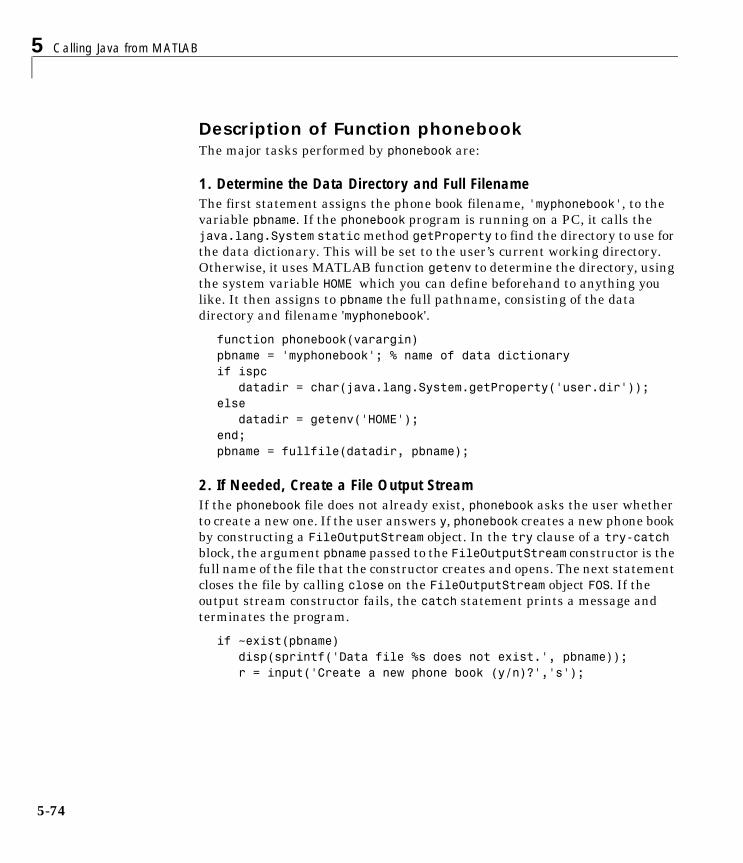
5 Calling Java from MATLAB
5-74
Description of Function phonebookThe major tasks performed by phonebook are:
1. Determine the Data Directory and Full FilenameThe first statement assigns the phone book filename, 'myphonebook', to the variable pbname. If the phonebook program is running on a PC, it calls the java.lang.System static method getProperty to find the directory to use for the data dictionary. This will be set to the user’s current working directory. Otherwise, it uses MATLAB function getenv to determine the directory, using the system variable HOME which you can define beforehand to anything you like. It then assigns to pbname the full pathname, consisting of the data directory and filename 'myphonebook'.
function phonebook(varargin)pbname = 'myphonebook'; % name of data dictionaryif ispc datadir = char(java.lang.System.getProperty('user.dir'));else datadir = getenv('HOME');end;pbname = fullfile(datadir, pbname);
2. If Needed, Create a File Output StreamIf the phonebook file does not already exist, phonebook asks the user whether to create a new one. If the user answers y, phonebook creates a new phone book by constructing a FileOutputStream object. In the try clause of a try-catch block, the argument pbname passed to the FileOutputStream constructor is the full name of the file that the constructor creates and opens. The next statement closes the file by calling close on the FileOutputStream object FOS. If the output stream constructor fails, the catch statement prints a message and terminates the program.
if ~exist(pbname) disp(sprintf('Data file %s does not exist.', pbname)); r = input('Create a new phone book (y/n)?','s');
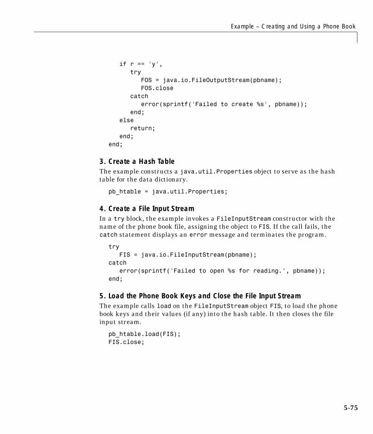
Example – Creating and Using a Phone Book
5-75
if r == 'y', try FOS = java.io.FileOutputStream(pbname); FOS.close catch error(sprintf('Failed to create %s', pbname)); end; else return; end;end;
3. Create a Hash TableThe example constructs a java.util.Properties object to serve as the hash table for the data dictionary.
pb_htable = java.util.Properties;
4. Create a File Input StreamIn a try block, the example invokes a FileInputStream constructor with the name of the phone book file, assigning the object to FIS. If the call fails, the catch statement displays an error message and terminates the program.
try FIS = java.io.FileInputStream(pbname);catch error(sprintf('Failed to open %s for reading.', pbname));end;
5. Load the Phone Book Keys and Close the File Input StreamThe example calls load on the FileInputStream object FIS, to load the phone book keys and their values (if any) into the hash table. It then closes the file input stream.
pb_htable.load(FIS);FIS.close;
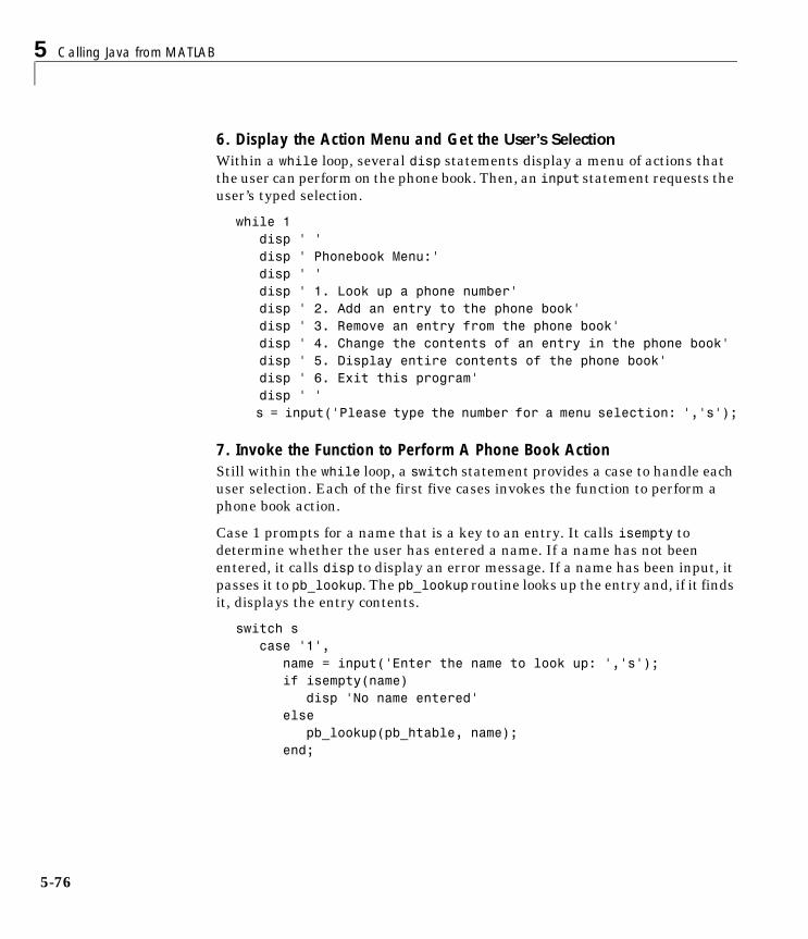
5 Calling Java from MATLAB
5-76
6. Display the Action Menu and Get the User’s SelectionWithin a while loop, several disp statements display a menu of actions that the user can perform on the phone book. Then, an input statement requests the user’s typed selection.
while 1 disp ' ' disp ' Phonebook Menu:' disp ' ' disp ' 1. Look up a phone number' disp ' 2. Add an entry to the phone book' disp ' 3. Remove an entry from the phone book' disp ' 4. Change the contents of an entry in the phone book' disp ' 5. Display entire contents of the phone book' disp ' 6. Exit this program' disp ' ' s = input('Please type the number for a menu selection: ','s');
7. Invoke the Function to Perform A Phone Book ActionStill within the while loop, a switch statement provides a case to handle each user selection. Each of the first five cases invokes the function to perform a phone book action.
Case 1 prompts for a name that is a key to an entry. It calls isempty to determine whether the user has entered a name. If a name has not been entered, it calls disp to display an error message. If a name has been input, it passes it to pb_lookup. The pb_lookup routine looks up the entry and, if it finds it, displays the entry contents.
switch s case '1', name = input('Enter the name to look up: ','s'); if isempty(name) disp 'No name entered' else pb_lookup(pb_htable, name); end;
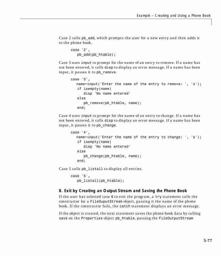
Example – Creating and Using a Phone Book
5-77
Case 2 calls pb_add, which prompts the user for a new entry and then adds it to the phone book.
case '2', pb_add(pb_htable);
Case 3 uses input to prompt for the name of an entry to remove. If a name has not been entered, it calls disp to display an error message. If a name has been input, it passes it to pb_remove.
case '3', name=input('Enter the name of the entry to remove: ', 's'); if isempty(name) disp 'No name entered' else pb_remove(pb_htable, name); end;
Case 4 uses input to prompt for the name of an entry to change. If a name has not been entered, it calls disp to display an error message. If a name has been input, it passes it to pb_change.
case '4', name=input('Enter the name of the entry to change: ', 's'); if isempty(name) disp 'No name entered' else pb_change(pb_htable, name); end;
Case 5 calls pb_listall to display all entries.
case '5', pb_listall(pb_htable);
8. Exit by Creating an Output Stream and Saving the Phone BookIf the user has selected case 6 to exit the program, a try statement calls the constructor for a FileOuputStream object, passing it the name of the phone book. If the constructor fails, the catch statement displays an error message.
If the object is created, the next statement saves the phone book data by calling save on the Properties object pb_htable, passing the FileOutputStream
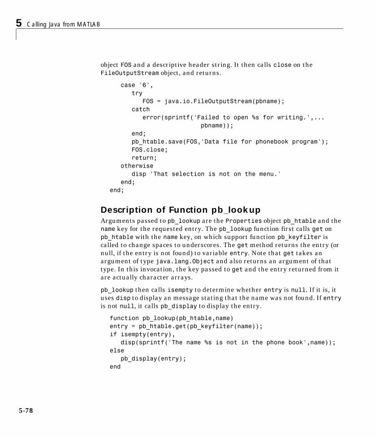
5 Calling Java from MATLAB
5-78
object FOS and a descriptive header string. It then calls close on the FileOutputStream object, and returns.
case '6', try FOS = java.io.FileOutputStream(pbname); catch error(sprintf('Failed to open %s for writing.',... pbname)); end; pb_htable.save(FOS,'Data file for phonebook program'); FOS.close; return; otherwise disp 'That selection is not on the menu.' end;end;
Description of Function pb_lookupArguments passed to pb_lookup are the Properties object pb_htable and the name key for the requested entry. The pb_lookup function first calls get on pb_htable with the name key, on which support function pb_keyfilter is called to change spaces to underscores. The get method returns the entry (or null, if the entry is not found) to variable entry. Note that get takes an argument of type java.lang.Object and also returns an argument of that type. In this invocation, the key passed to get and the entry returned from it are actually character arrays.
pb_lookup then calls isempty to determine whether entry is null. If it is, it uses disp to display an message stating that the name was not found. If entry is not null, it calls pb_display to display the entry.
function pb_lookup(pb_htable,name)entry = pb_htable.get(pb_keyfilter(name));if isempty(entry), disp(sprintf('The name %s is not in the phone book',name));else pb_display(entry);end
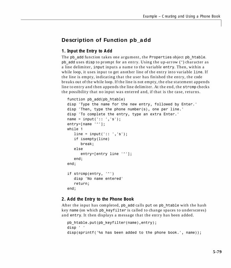
Example – Creating and Using a Phone Book
5-79
Description of Function pb_add
1. Input the Entry to AddThe pb_add function takes one argument, the Properties object pb_htable. pb_add uses disp to prompt for an entry. Using the up-arrow (^) character as a line delimiter, input inputs a name to the variable entry. Then, within a while loop, it uses input to get another line of the entry into variable line. If the line is empty, indicating that the user has finished the entry, the code breaks out of the while loop. If the line is not empty, the else statement appends line to entry and then appends the line delimiter. At the end, the strcmp checks the possibility that no input was entered and, if that is the case, returns.
function pb_add(pb_htable)disp 'Type the name for the new entry, followed by Enter.'disp 'Then, type the phone number(s), one per line.'disp 'To complete the entry, type an extra Enter.'name = input(':: ','s');entry=[name '^'];while 1 line = input(':: ','s'); if isempty(line) break; else entry=[entry line '^']; end;end;
if strcmp(entry, '^') disp 'No name entered' return;end;
2. Add the Entry to the Phone BookAfter the input has completed, pb_add calls put on pb_htable with the hash key name (on which pb_keyfilter is called to change spaces to underscores) and entry. It then displays a message that the entry has been added.
pb_htable.put(pb_keyfilter(name),entry);disp ' 'disp(sprintf('%s has been added to the phone book.', name));
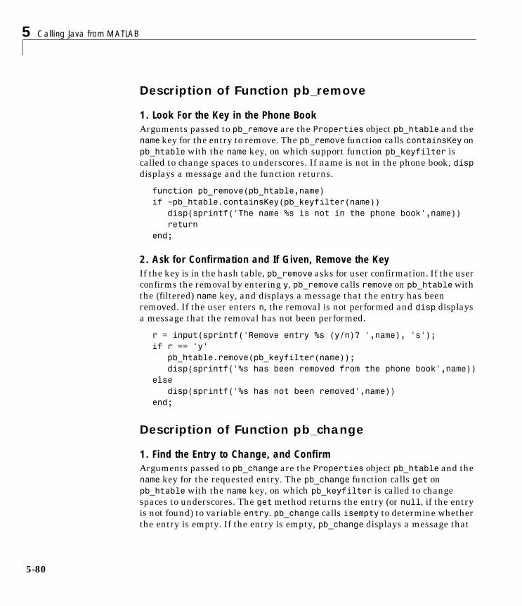
5 Calling Java from MATLAB
5-80
Description of Function pb_remove
1. Look For the Key in the Phone BookArguments passed to pb_remove are the Properties object pb_htable and the name key for the entry to remove. The pb_remove function calls containsKey on pb_htable with the name key, on which support function pb_keyfilter is called to change spaces to underscores. If name is not in the phone book, disp displays a message and the function returns.
function pb_remove(pb_htable,name)if ~pb_htable.containsKey(pb_keyfilter(name)) disp(sprintf('The name %s is not in the phone book',name)) returnend;
2. Ask for Confirmation and If Given, Remove the KeyIf the key is in the hash table, pb_remove asks for user confirmation. If the user confirms the removal by entering y, pb_remove calls remove on pb_htable with the (filtered) name key, and displays a message that the entry has been removed. If the user enters n, the removal is not performed and disp displays a message that the removal has not been performed.
r = input(sprintf('Remove entry %s (y/n)? ',name), 's');if r == 'y' pb_htable.remove(pb_keyfilter(name)); disp(sprintf('%s has been removed from the phone book',name))else disp(sprintf('%s has not been removed',name))end;
Description of Function pb_change
1. Find the Entry to Change, and ConfirmArguments passed to pb_change are the Properties object pb_htable and the name key for the requested entry. The pb_change function calls get on pb_htable with the name key, on which pb_keyfilter is called to change spaces to underscores. The get method returns the entry (or null, if the entry is not found) to variable entry. pb_change calls isempty to determine whether the entry is empty. If the entry is empty, pb_change displays a message that
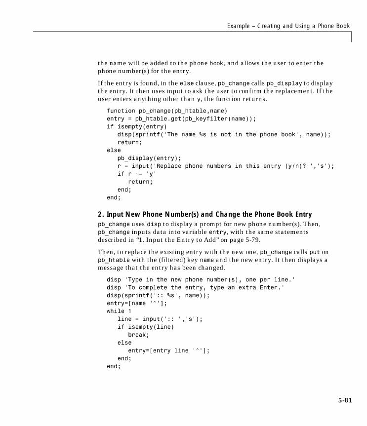
Example – Creating and Using a Phone Book
5-81
the name will be added to the phone book, and allows the user to enter the phone number(s) for the entry.
If the entry is found, in the else clause, pb_change calls pb_display to display the entry. It then uses input to ask the user to confirm the replacement. If the user enters anything other than y, the function returns.
function pb_change(pb_htable,name)entry = pb_htable.get(pb_keyfilter(name));if isempty(entry) disp(sprintf('The name %s is not in the phone book', name)); return;else pb_display(entry); r = input('Replace phone numbers in this entry (y/n)? ','s'); if r ~= 'y' return; end;end;
2. Input New Phone Number(s) and Change the Phone Book Entrypb_change uses disp to display a prompt for new phone number(s). Then, pb_change inputs data into variable entry, with the same statements described in “1. Input the Entry to Add” on page 5-79.
Then, to replace the existing entry with the new one, pb_change calls put on pb_htable with the (filtered) key name and the new entry. It then displays a message that the entry has been changed.
disp 'Type in the new phone number(s), one per line.'disp 'To complete the entry, type an extra Enter.'disp(sprintf(':: %s', name));entry=[name '^'];while 1 line = input(':: ','s'); if isempty(line) break; else entry=[entry line '^']; end;end;
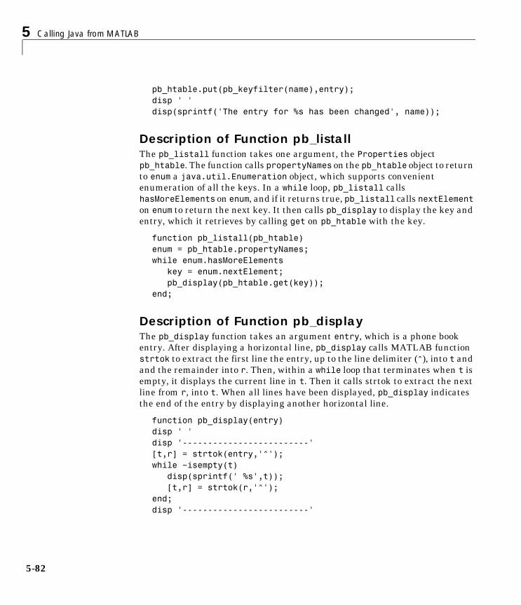
5 Calling Java from MATLAB
5-82
pb_htable.put(pb_keyfilter(name),entry);disp ' 'disp(sprintf('The entry for %s has been changed', name));
Description of Function pb_listallThe pb_listall function takes one argument, the Properties object pb_htable. The function calls propertyNames on the pb_htable object to return to enum a java.util.Enumeration object, which supports convenient enumeration of all the keys. In a while loop, pb_listall calls hasMoreElements on enum, and if it returns true, pb_listall calls nextElement on enum to return the next key. It then calls pb_display to display the key and entry, which it retrieves by calling get on pb_htable with the key.
function pb_listall(pb_htable)enum = pb_htable.propertyNames;while enum.hasMoreElements key = enum.nextElement; pb_display(pb_htable.get(key));end;
Description of Function pb_displayThe pb_display function takes an argument entry, which is a phone book entry. After displaying a horizontal line, pb_display calls MATLAB function strtok to extract the first line the entry, up to the line delimiter (^), into t and and the remainder into r. Then, within a while loop that terminates when t is empty, it displays the current line in t. Then it calls strtok to extract the next line from r, into t. When all lines have been displayed, pb_display indicates the end of the entry by displaying another horizontal line.
function pb_display(entry)disp ' 'disp '-------------------------'[t,r] = strtok(entry,'^');while ~isempty(t) disp(sprintf(' %s',t)); [t,r] = strtok(r,'^');end;disp '-------------------------'
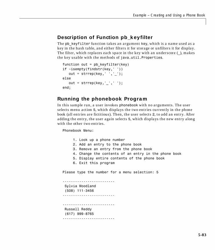
Example – Creating and Using a Phone Book
5-83
Description of Function pb_keyfilterThe pb_keyfilter function takes an argument key, which is a name used as a key in the hash table, and either filters it for storage or unfilters it for display. The filter, which replaces each space in the key with an underscore (_), makes the key usable with the methods of java.util.Properties.
function out = pb_keyfilter(key)if ~isempty(findstr(key,' ')) out = strrep(key,' ','_');else out = strrep(key,'_',' ');end;
Running the phonebook ProgramIn this sample run, a user invokes phonebook with no arguments. The user selects menu action 5, which displays the two entries currently in the phone book (all entries are fictitious). Then, the user selects 2, to add an entry. After adding the entry, the user again selects 5, which displays the new entry along with the other two entries.
Phonebook Menu: 1. Look up a phone number 2. Add an entry to the phone book 3. Remove an entry from the phone book 4. Change the contents of an entry in the phone book 5. Display entire contents of the phone book 6. Exit this program Please type the number for a menu selection: 5 ------------------------- Sylvia Woodland (508) 111-3456------------------------- ------------------------- Russell Reddy (617) 999-8765-------------------------
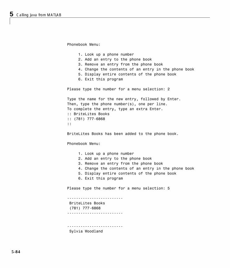
5 Calling Java from MATLAB
5-84
Phonebook Menu: 1. Look up a phone number 2. Add an entry to the phone book 3. Remove an entry from the phone book 4. Change the contents of an entry in the phone book 5. Display entire contents of the phone book 6. Exit this program Please type the number for a menu selection: 2 Type the name for the new entry, followed by Enter.Then, type the phone number(s), one per line.To complete the entry, type an extra Enter.:: BriteLites Books:: (781) 777-6868:: BriteLites Books has been added to the phone book.
Phonebook Menu: 1. Look up a phone number 2. Add an entry to the phone book 3. Remove an entry from the phone book 4. Change the contents of an entry in the phone book 5. Display entire contents of the phone book 6. Exit this program Please type the number for a menu selection: 5 ------------------------- BriteLites Books (781) 777-6868-------------------------
------------------------- Sylvia Woodland
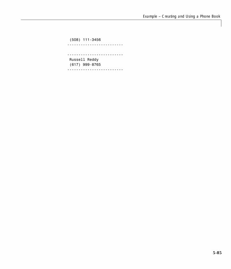
Example – Creating and Using a Phone Book
5-85
(508) 111-3456------------------------- ------------------------- Russell Reddy (617) 999-8765-------------------------

5 Calling Java from MATLAB
5-86
6Importing and Exporting Data
Using MAT-Files . . . . . . . . . . . . . . . . . . 6-3Importing Data to MATLAB . . . . . . . . . . . . . . 6-3Exporting Data from MATLAB . . . . . . . . . . . . . 6-4Exchanging Data Files Between Platforms . . . . . . . . 6-5Reading and Writing MAT-Files . . . . . . . . . . . . 6-6Finding Associated Files . . . . . . . . . . . . . . . . 6-8
Examples of MAT-Files . . . . . . . . . . . . . . . 6-11Creating a MAT-File in C . . . . . . . . . . . . . . . 6-11Reading a MAT-File in C . . . . . . . . . . . . . . . 6-16Creating a MAT-File in Fortran . . . . . . . . . . . . . 6-21Reading a MAT-File in Fortran . . . . . . . . . . . . . 6-24
Compiling and Linking MAT-File Programs . . . . . . 6-28Masking Floating Point Exceptions . . . . . . . . . . . 6-28Compiling and Linking on UNIX . . . . . . . . . . . . 6-29Compiling and Linking on Windows . . . . . . . . . . . 6-30
6 Importing and Exporting Data
6-2
You can use MAT-files, the data file format MATLAB uses for saving data to disk, to import data to and export data from the MATLAB environment. MAT-files provide a convenient mechanism for moving your MATLAB data between different platforms in a highly portable manner. In addition, they provide a means to import and export your data to other stand-alone MATLAB applications.
To simplify your use of MAT-files in applications outside of MATLAB, we provide a library of access routines that you can use in your own C or Fortran programs to read and write MAT-files. Programs that access MAT-files also use the mx API routines discussed in this book.
The following list summarizes the contents of this chapter:
• “Using MAT-Files”
• “Examples of MAT-Files”
• “Compiling and Linking MAT-File Programs”
For additional information and support in building your applications, see the section entitled, “Additional Information” on page 1-42.
Using MAT-Files
6-3
Using MAT-FilesThis section describes the various techniques for importing data to and exporting data from the MATLAB environment. The main topics that are discussed are:
• “Importing Data to MATLAB”
• “Exporting Data from MATLAB”
• “Exchanging Data Files Between Platforms”
• “Reading and Writing MAT-Files”
• “Finding Associated Files”
The most important approach to importing and exporting data involves the use of MAT-files, the data file format that MATLAB uses for saving data to your disk. MAT-files provide a convenient mechanism for moving your MATLAB data between different platforms and for importing and exporting your data to other stand-alone MATLAB applications.
To simplify your use of MAT-files in applications outside of MATLAB, we have developed a library of access routines with a mat prefix that you can use in your own C or Fortran programs to read and write MAT-files. Programs that access MAT-files also use the mx prefixed API routines discussed in Chapter 2, “Creating C Language MEX-Files” and Chapter 3, “Creating Fortran MEX-Files.”
Importing Data to MATLABYou can introduce data from other programs into MATLAB by several methods. The best method for importing data depends on how much data there is, whether the data is already in machine-readable form, and what format the data is in. Here are some choices. Select the one that best meets your needs.
• Enter the data as an explicit list of elements.
If you have a small amount of data, less than 10-15 elements, it is easy to type the data explicitly using brackets [ ]. This method is awkward for larger amounts of data because you can’t edit your input if you make a mistake.
• Create data in an M-file.
Use your text editor to create an M-file that enters your data as an explicit list of elements. This method is useful when the data isn’t already in
6 Importing and Exporting Data
6-4
computer-readable form and you have to type it in. Essentially the same as the first method, this method has the advantage of allowing you to use your editor to change the data and correct mistakes. You can then just rerun your M-file to re-enter the data.
• Load data from an ASCII flat file.
A flat file stores the data in ASCII form, with fixed-length rows terminated with new lines (carriage returns) and with spaces separating the numbers. You can edit ASCII flat files using a normal text editor. Flat files can be read directly into MATLAB using the load command. The result is to create a variable with the same name as the filename.
See the load function reference page for more information.
• Read data using MATLAB’s I/O functions.
You can read data using fopen, fread, and MATLAB’s other low-level I/O functions. This method is useful for loading data files from other applications that have their own established file formats.
• Write a MEX-file to read the data.
This is the method of choice if subroutines are already available for reading data files from other applications. See the section, “Introducing MEX-Files” on page 1-3, for more information.
• Write a program to translate your data.
You can write a program in C or Fortran to translate your data into MAT-file format. You can then read the MAT-file into MATLAB using the load command. Refer to the section, “Reading and Writing MAT-Files” on page 6-6, for more information.
Exporting Data from MATLABThere are several methods for getting MATLAB data back to the outside world:
• Create a diary file.
For small matrices, use the diary command to create a diary file and display the variables, echoing them into this file. You can use your text editor to manipulate the diary file at a later time. The output of diary includes the MATLAB commands used during the session, which is useful for inclusion into documents and reports.
Using MAT-Files
6-5
• Use the Save command.
Save the data in ASCII form using the save command with the -ascii option. For example,A = rand(4,3);
save temp.dat A -ascii
creates an ASCII file called temp.dat containing1.3889088e-001 2.7218792e-001 4.4509643e-0012.0276522e-001 1.9881427e-001 9.3181458e-0011.9872174e-001 1.5273927e-002 4.6599434e-0016.0379248e-001 7.4678568e-001 4.1864947e-001
The -ascii option supports two-dimensional double and character arrays only. Multidimensional arrays, cell arrays, and structures are not supported.
See the save function reference page for more information.
• Use MATLAB I/O functions.
Write the data in a special format using fopen, fwrite, and the other low-level I/O functions. This method is useful for writing data files in the file formats required by other applications.
• Develop a MEX-file to write the data.
You can develop a MEX-file to write the data. This is the method of choice if subroutines are already available for writing data files in the form needed by other applications. See the section, “Introducing MEX-Files” on page 1-3, for more information.
• Translate data from a MAT-file.
You can write out the data as a MAT-file using the save command. You can then write a program in C or Fortran to translate the MAT-file into your own special format. See the section, “Reading and Writing MAT-Files” on page 6-6, for more information.
Exchanging Data Files Between PlatformsYou may want to work with MATLAB implementations on several different computer systems, or need to transmit MATLAB applications to users on other systems. MATLAB applications consist of M-files containing functions and scripts, and MAT-files containing binary data.
6 Importing and Exporting Data
6-6
Both types of files can be transported directly between machines: M-files because they are platform independent and MAT-files because they contain a machine signature in the file header. MATLAB checks the signature when it loads a file and, if a signature indicates that a file is foreign, performs the necessary conversion.
Using MATLAB across several different machine architectures requires a facility for exchanging both binary and ASCII data between the various machines. Examples of this type of facility include FTP, NFS, Kermit, and other communication programs. When using these programs, be careful to transmit binary MAT-files in binary file mode and ASCII M-files in ASCII file mode. Failure to set these modes correctly corrupts the data.
Reading and Writing MAT-FilesThe save command in MATLAB saves the MATLAB arrays currently in memory to a binary disk file called a MAT-file. The term MAT-file is used because these files have the extension .mat. The load command performs the reverse operation. It reads the MATLAB arrays from a MAT-file on disk back into MATLAB’s workspace.
A MAT-file may contain one or more of any of the data types supported in MATLAB 5 or later, including strings, matrices, multidimensional arrays, structures, and cell arrays. MATLAB writes the data sequentially onto disk as a continuous byte stream.
MAT-File Interface LibraryThe MAT-file interface library contains a set of routines for reading and writing MAT-files. You can call these routines from within your own C and Fortran programs. We recommend that you use these routines, rather than attempt to write your own code, to perform these operations. By using the routines in this library, you will be insulated from future changes to the MAT-file structure.
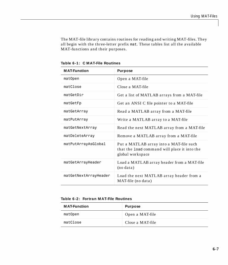
Using MAT-Files
6-7
The MAT-file library contains routines for reading and writing MAT-files. They all begin with the three-letter prefix mat. These tables list all the available MAT-functions and their purposes.
Table 6-1: C MAT-File Routines
MAT-Function Purpose
matOpen Open a MAT-file
matClose Close a MAT-file
matGetDir Get a list of MATLAB arrays from a MAT-file
matGetFp Get an ANSI C file pointer to a MAT-file
matGetArray Read a MATLAB array from a MAT-file
matPutArray Write a MATLAB array to a MAT-file
matGetNextArray Read the next MATLAB array from a MAT-file
matDeleteArray Remove a MATLAB array from a MAT-file
matPutArrayAsGlobal Put a MATLAB array into a MAT-file such that the load command will place it into the global workspace
matGetArrayHeader Load a MATLAB array header from a MAT-file (no data)
matGetNextArrayHeader Load the next MATLAB array header from a MAT-file (no data)
Table 6-2: Fortran MAT-File Routines
MAT-Function Purpose
matOpen Open a MAT-file
matClose Close a MAT-file
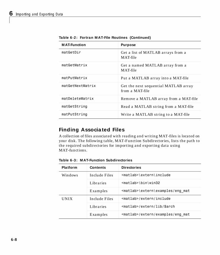
6 Importing and Exporting Data
6-8
Finding Associated FilesA collection of files associated with reading and writing MAT-files is located on your disk. The following table, MAT-Function Subdirectories, lists the path to the required subdirectories for importing and exporting data using MAT-functions.
matGetDir Get a list of MATLAB arrays from a MAT-file
matGetMatrix Get a named MATLAB array from a MAT-file
matPutMatrix Put a MATLAB array into a MAT-file
matGetNextMatrix Get the next sequential MATLAB array from a MAT-file
matDeleteMatrix Remove a MATLAB array from a MAT-file
matGetString Read a MATLAB string from a MAT-file
matPutString Write a MATLAB string to a MAT-file
Table 6-3: MAT-Function Subdirectories
Platform Contents Directories
Windows Include Files <matlab>\extern\include
Libraries <matlab>\bin\win32
Examples <matlab>\extern\examples/eng_mat
UNIX Include Files <matlab>/extern/include
Libraries <matlab>/extern/lib/$arch
Examples <matlab>/extern/examples/eng_mat
Table 6-2: Fortran MAT-File Routines (Continued)
MAT-Function Purpose
Using MAT-Files
6-9
Include FilesThe include directory holds header files containing function declarations with prototypes for the routines that you can access in the API Library. These files are the same for both Windows and UNIX. Included in the subdirectory are:
• matrix.h, the header file that defines MATLAB array access and creation methods
• mat.h, the header file that defines MAT-file access and creation methods
LibrariesThe subdirectory that contains shared (dynamically linkable) libraries for linking your programs is platform dependent.
Shared Libraries on Windows. The bin subdirectory contains the shared libraries for linking your programs:
• libmat.dll, the library of MAT-file routines (C and Fortran)
• libmx.dll, the library of array access and creation routines
Shared Libraries on UNIX. The extern/lib/$arch subdirectory, where $arch is your machine’s architecture, contains the shared libraries for linking your programs. For example, on sol2, the subdirectory is extern/lib/sol2:
• libmat.so, the library of MAT-file routines (C and Fortran)
• libmx.so, the library of array access and creation routines
Example FilesThe examples/eng_mat subdirectory contains C and Fortran source code for a number of example files that demonstrate how to use the MAT-file routines. The source code files are the same for both Windows and UNIX.
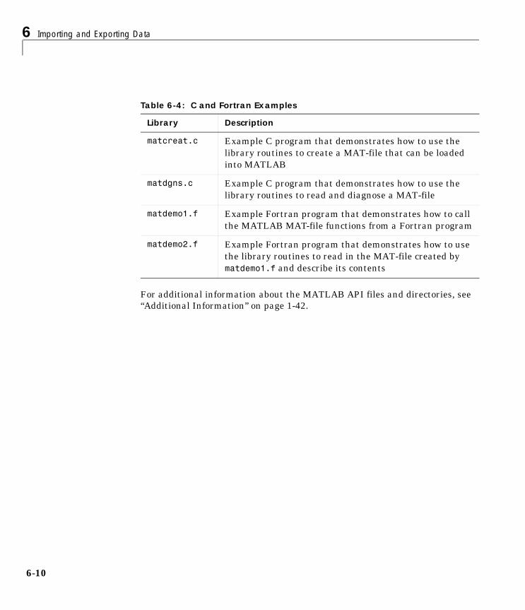
6 Importing and Exporting Data
6-10
For additional information about the MATLAB API files and directories, see “Additional Information” on page 1-42.
Table 6-4: C and Fortran Examples
Library Description
matcreat.c Example C program that demonstrates how to use the library routines to create a MAT-file that can be loaded into MATLAB
matdgns.c Example C program that demonstrates how to use the library routines to read and diagnose a MAT-file
matdemo1.f Example Fortran program that demonstrates how to call the MATLAB MAT-file functions from a Fortran program
matdemo2.f Example Fortran program that demonstrates how to use the library routines to read in the MAT-file created by matdemo1.f and describe its contents
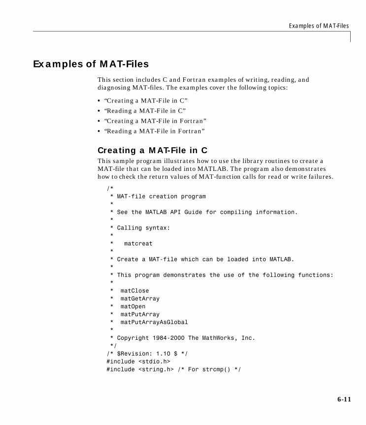
Examples of MAT-Files
6-11
Examples of MAT-FilesThis section includes C and Fortran examples of writing, reading, and diagnosing MAT-files. The examples cover the following topics:
• “Creating a MAT-File in C”
• “Reading a MAT-File in C”
• “Creating a MAT-File in Fortran”
• “Reading a MAT-File in Fortran”
Creating a MAT-File in CThis sample program illustrates how to use the library routines to create a MAT-file that can be loaded into MATLAB. The program also demonstrates how to check the return values of MAT-function calls for read or write failures.
/* * MAT-file creation program * * See the MATLAB API Guide for compiling information. * * Calling syntax: * * matcreat * * Create a MAT-file which can be loaded into MATLAB. * * This program demonstrates the use of the following functions: * * matClose * matGetArray * matOpen * matPutArray * matPutArrayAsGlobal * * Copyright 1984-2000 The MathWorks, Inc. *//* $Revision: 1.10 $ */#include <stdio.h>#include <string.h> /* For strcmp() */
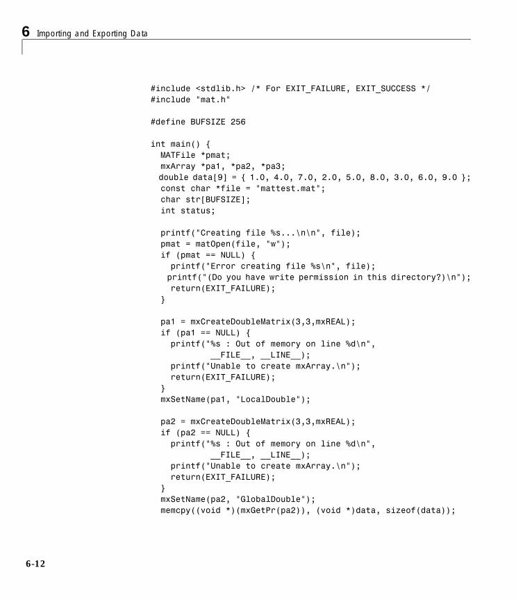
6 Importing and Exporting Data
6-12
#include <stdlib.h> /* For EXIT_FAILURE, EXIT_SUCCESS */#include "mat.h"
#define BUFSIZE 256
int main() { MATFile *pmat; mxArray *pa1, *pa2, *pa3; double data[9] = { 1.0, 4.0, 7.0, 2.0, 5.0, 8.0, 3.0, 6.0, 9.0 }; const char *file = "mattest.mat"; char str[BUFSIZE]; int status;
printf("Creating file %s...\n\n", file); pmat = matOpen(file, "w"); if (pmat == NULL) { printf("Error creating file %s\n", file); printf("(Do you have write permission in this directory?)\n"); return(EXIT_FAILURE); }
pa1 = mxCreateDoubleMatrix(3,3,mxREAL); if (pa1 == NULL) { printf("%s : Out of memory on line %d\n", __FILE__, __LINE__); printf("Unable to create mxArray.\n"); return(EXIT_FAILURE); } mxSetName(pa1, "LocalDouble");
pa2 = mxCreateDoubleMatrix(3,3,mxREAL); if (pa2 == NULL) { printf("%s : Out of memory on line %d\n", __FILE__, __LINE__); printf("Unable to create mxArray.\n"); return(EXIT_FAILURE); } mxSetName(pa2, "GlobalDouble"); memcpy((void *)(mxGetPr(pa2)), (void *)data, sizeof(data));
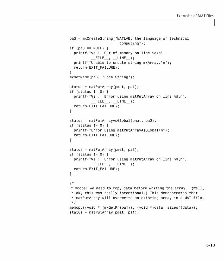
Examples of MAT-Files
6-13
pa3 = mxCreateString("MATLAB: the language of technical computing"); if (pa3 == NULL) { printf("%s : Out of memory on line %d\n", __FILE__, __LINE__); printf("Unable to create string mxArray.\n"); return(EXIT_FAILURE); } mxSetName(pa3, "LocalString");
status = matPutArray(pmat, pa1); if (status != 0) { printf("%s : Error using matPutArray on line %d\n", __FILE__, __LINE__); return(EXIT_FAILURE); } status = matPutArrayAsGlobal(pmat, pa2); if (status != 0) { printf("Error using matPutArrayAsGlobal\n"); return(EXIT_FAILURE); } status = matPutArray(pmat, pa3); if (status != 0) { printf("%s : Error using matPutArray on line %d\n", __FILE__, __LINE__); return(EXIT_FAILURE); } /* * Ooops! we need to copy data before writing the array. (Well, * ok, this was really intentional.) This demonstrates that * matPutArray will overwrite an existing array in a MAT-file. */ memcpy((void *)(mxGetPr(pa1)), (void *)data, sizeof(data)); status = matPutArray(pmat, pa1);
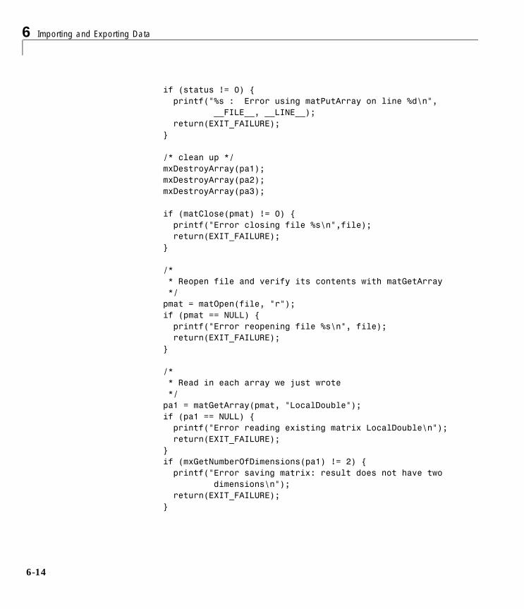
6 Importing and Exporting Data
6-14
if (status != 0) { printf("%s : Error using matPutArray on line %d\n", __FILE__, __LINE__); return(EXIT_FAILURE); } /* clean up */ mxDestroyArray(pa1); mxDestroyArray(pa2); mxDestroyArray(pa3);
if (matClose(pmat) != 0) { printf("Error closing file %s\n",file); return(EXIT_FAILURE); }
/* * Reopen file and verify its contents with matGetArray */ pmat = matOpen(file, "r"); if (pmat == NULL) { printf("Error reopening file %s\n", file); return(EXIT_FAILURE); }
/* * Read in each array we just wrote */ pa1 = matGetArray(pmat, "LocalDouble"); if (pa1 == NULL) { printf("Error reading existing matrix LocalDouble\n"); return(EXIT_FAILURE); } if (mxGetNumberOfDimensions(pa1) != 2) { printf("Error saving matrix: result does not have two dimensions\n"); return(EXIT_FAILURE); }
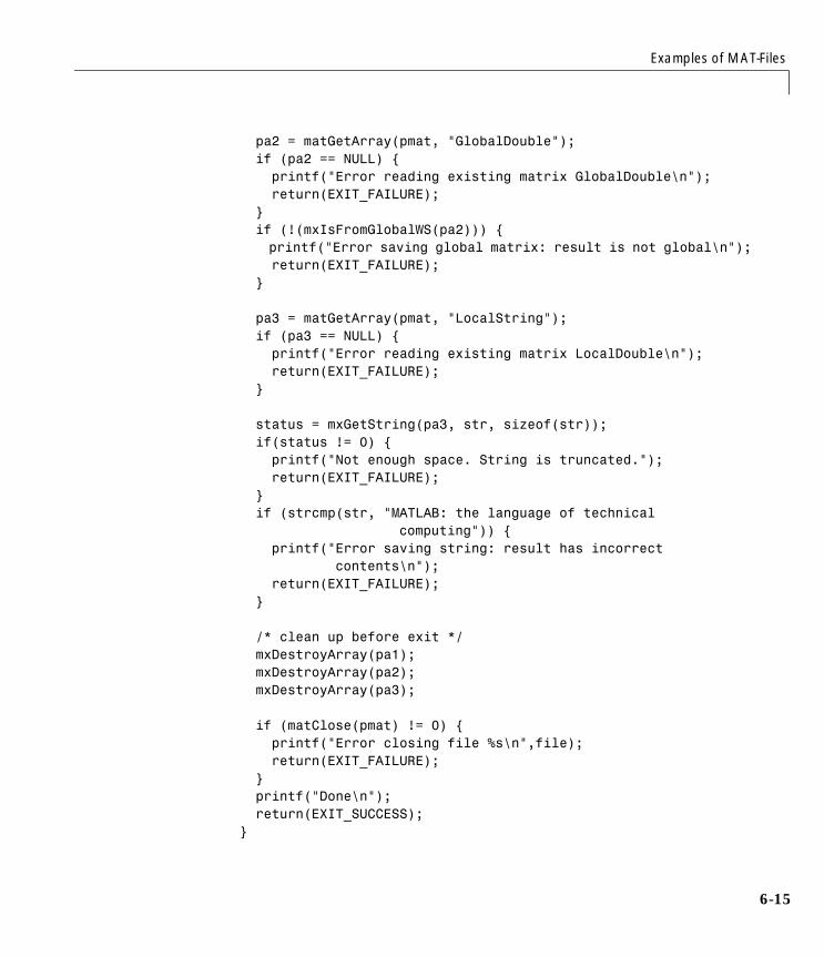
Examples of MAT-Files
6-15
pa2 = matGetArray(pmat, "GlobalDouble"); if (pa2 == NULL) { printf("Error reading existing matrix GlobalDouble\n"); return(EXIT_FAILURE); } if (!(mxIsFromGlobalWS(pa2))) { printf("Error saving global matrix: result is not global\n"); return(EXIT_FAILURE); }
pa3 = matGetArray(pmat, "LocalString"); if (pa3 == NULL) { printf("Error reading existing matrix LocalDouble\n"); return(EXIT_FAILURE); } status = mxGetString(pa3, str, sizeof(str)); if(status != 0) { printf("Not enough space. String is truncated."); return(EXIT_FAILURE); } if (strcmp(str, "MATLAB: the language of technical computing")) { printf("Error saving string: result has incorrect contents\n"); return(EXIT_FAILURE); }
/* clean up before exit */ mxDestroyArray(pa1); mxDestroyArray(pa2); mxDestroyArray(pa3);
if (matClose(pmat) != 0) { printf("Error closing file %s\n",file); return(EXIT_FAILURE); } printf("Done\n"); return(EXIT_SUCCESS);}
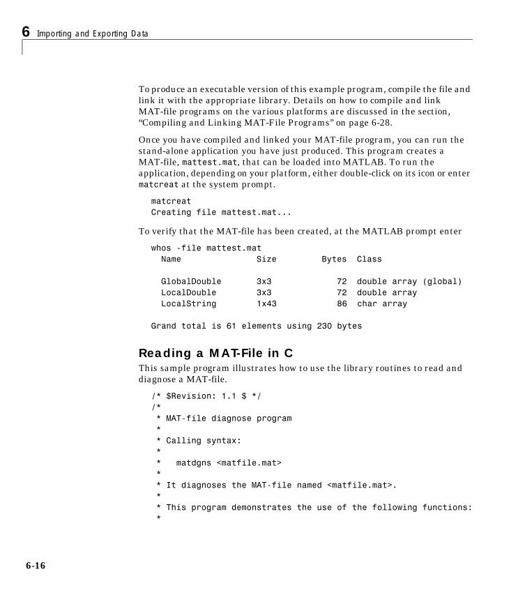
6 Importing and Exporting Data
6-16
To produce an executable version of this example program, compile the file and link it with the appropriate library. Details on how to compile and link MAT-file programs on the various platforms are discussed in the section, “Compiling and Linking MAT-File Programs” on page 6-28.
Once you have compiled and linked your MAT-file program, you can run the stand-alone application you have just produced. This program creates a MAT-file, mattest.mat, that can be loaded into MATLAB. To run the application, depending on your platform, either double-click on its icon or enter matcreat at the system prompt.
matcreatCreating file mattest.mat...
To verify that the MAT-file has been created, at the MATLAB prompt enter
whos -file mattest.mat Name Size Bytes Class
GlobalDouble 3x3 72 double array (global) LocalDouble 3x3 72 double array LocalString 1x43 86 char array
Grand total is 61 elements using 230 bytes
Reading a MAT-File in CThis sample program illustrates how to use the library routines to read and diagnose a MAT-file.
/* $Revision: 1.1 $ *//* * MAT-file diagnose program * * Calling syntax: * * matdgns <matfile.mat> * * It diagnoses the MAT-file named <matfile.mat>. * * This program demonstrates the use of the following functions: *
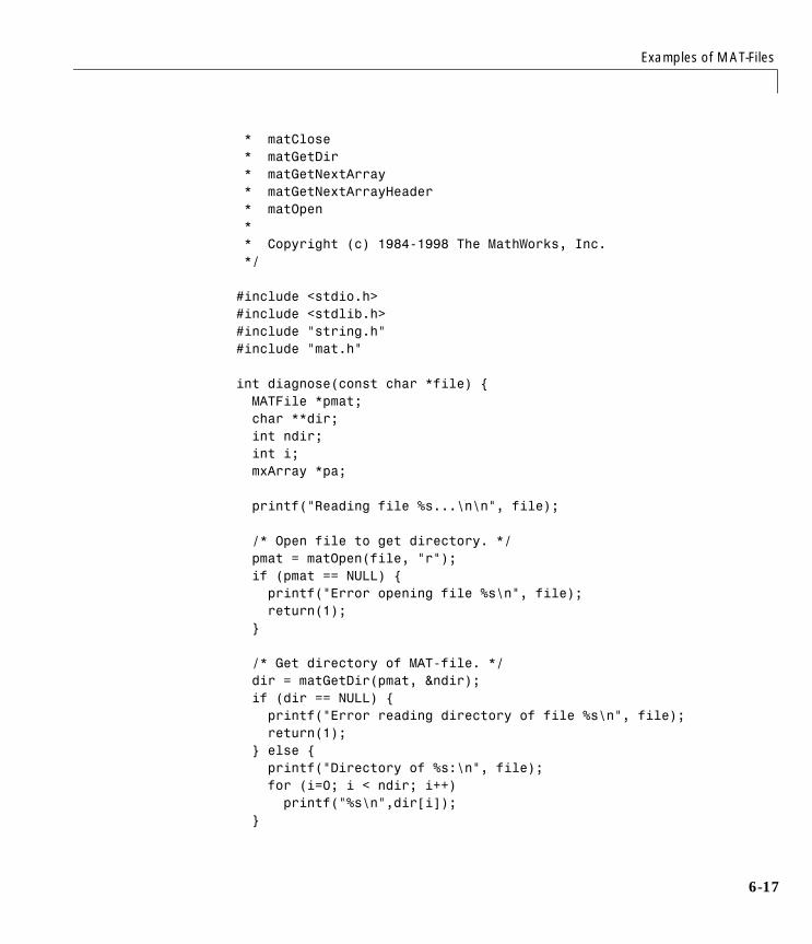
Examples of MAT-Files
6-17
* matClose * matGetDir * matGetNextArray * matGetNextArrayHeader * matOpen * * Copyright (c) 1984-1998 The MathWorks, Inc. */
#include <stdio.h>#include <stdlib.h>#include "string.h"#include "mat.h"
int diagnose(const char *file) { MATFile *pmat; char **dir; int ndir; int i; mxArray *pa; printf("Reading file %s...\n\n", file);
/* Open file to get directory. */ pmat = matOpen(file, "r"); if (pmat == NULL) { printf("Error opening file %s\n", file); return(1); } /* Get directory of MAT-file. */ dir = matGetDir(pmat, &ndir); if (dir == NULL) { printf("Error reading directory of file %s\n", file); return(1); } else { printf("Directory of %s:\n", file); for (i=0; i < ndir; i++) printf("%s\n",dir[i]); }
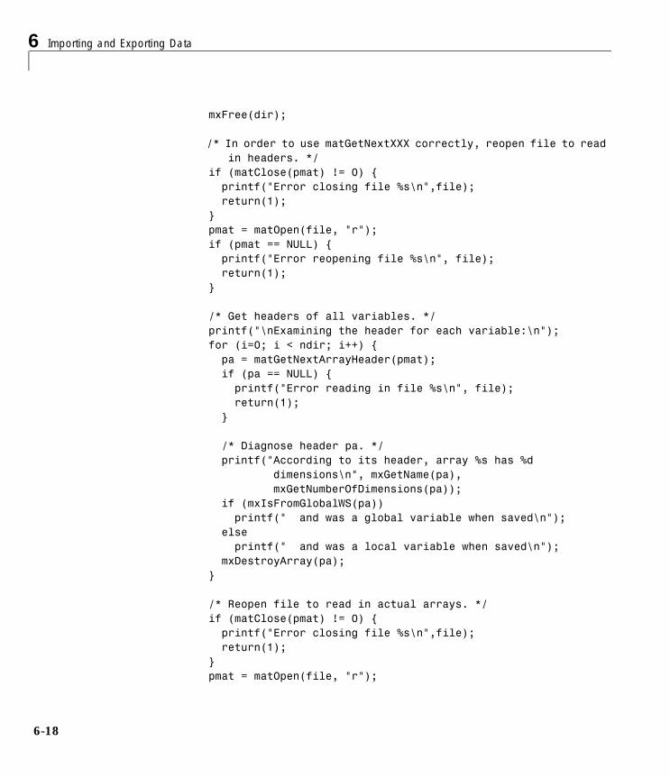
6 Importing and Exporting Data
6-18
mxFree(dir);
/* In order to use matGetNextXXX correctly, reopen file to read in headers. */ if (matClose(pmat) != 0) { printf("Error closing file %s\n",file); return(1); } pmat = matOpen(file, "r"); if (pmat == NULL) { printf("Error reopening file %s\n", file); return(1); }
/* Get headers of all variables. */ printf("\nExamining the header for each variable:\n"); for (i=0; i < ndir; i++) { pa = matGetNextArrayHeader(pmat); if (pa == NULL) { printf("Error reading in file %s\n", file); return(1); }
/* Diagnose header pa. */ printf("According to its header, array %s has %d dimensions\n", mxGetName(pa), mxGetNumberOfDimensions(pa)); if (mxIsFromGlobalWS(pa)) printf(" and was a global variable when saved\n"); else printf(" and was a local variable when saved\n"); mxDestroyArray(pa); }
/* Reopen file to read in actual arrays. */ if (matClose(pmat) != 0) { printf("Error closing file %s\n",file); return(1); } pmat = matOpen(file, "r");

Examples of MAT-Files
6-19
if (pmat == NULL) { printf("Error reopening file %s\n", file); return(1); }
/* Read in each array. */ printf("\nReading in the actual array contents:\n"); for (i=0; i<ndir; i++) { pa = matGetNextArray(pmat); if (pa == NULL) { printf("Error reading in file %s\n", file); return(1); }
/* Diagnose array pa. */ printf("According to its contents, array %s has %d dimensions\n", mxGetName(pa), mxGetNumberOfDimensions(pa)); if (mxIsFromGlobalWS(pa)) printf(" and was a global variable when saved\n"); else printf(" and was a local variable when saved\n"); mxDestroyArray(pa); }
if (matClose(pmat) != 0) { printf("Error closing file %s\n",file); return(1); } printf("Done\n"); return(0);}
int main(int argc, char **argv){ int result;
if (argc > 1) result = diagnose(argv[1]);
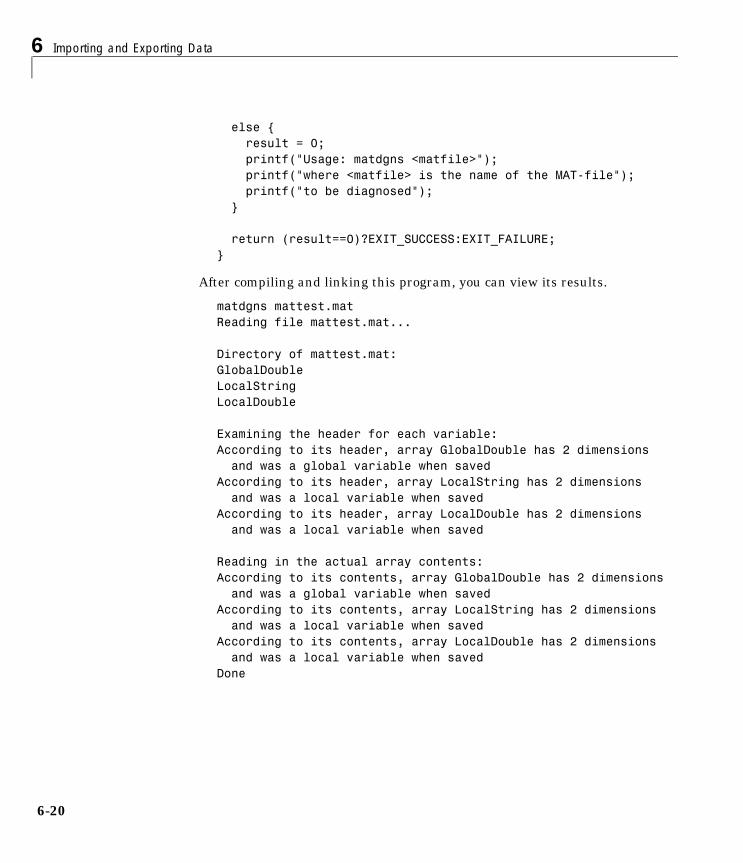
6 Importing and Exporting Data
6-20
else { result = 0; printf("Usage: matdgns <matfile>"); printf("where <matfile> is the name of the MAT-file"); printf("to be diagnosed"); }
return (result==0)?EXIT_SUCCESS:EXIT_FAILURE;}
After compiling and linking this program, you can view its results.
matdgns mattest.matReading file mattest.mat... Directory of mattest.mat:GlobalDoubleLocalStringLocalDouble Examining the header for each variable:According to its header, array GlobalDouble has 2 dimensions and was a global variable when savedAccording to its header, array LocalString has 2 dimensions and was a local variable when savedAccording to its header, array LocalDouble has 2 dimensions and was a local variable when saved Reading in the actual array contents:According to its contents, array GlobalDouble has 2 dimensions and was a global variable when savedAccording to its contents, array LocalString has 2 dimensions and was a local variable when savedAccording to its contents, array LocalDouble has 2 dimensions and was a local variable when savedDone
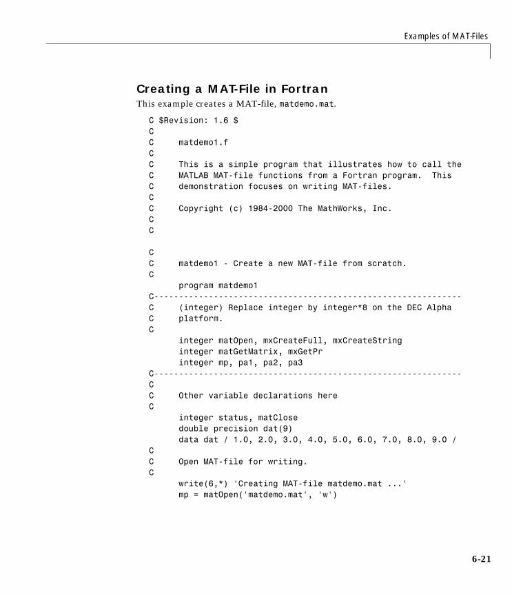
Examples of MAT-Files
6-21
Creating a MAT-File in FortranThis example creates a MAT-file, matdemo.mat.
C $Revision: 1.6 $CC matdemo1.fCC This is a simple program that illustrates how to call theC MATLAB MAT-file functions from a Fortran program. ThisC demonstration focuses on writing MAT-files.CC Copyright (c) 1984-2000 The MathWorks, Inc.C C
CC matdemo1 - Create a new MAT-file from scratch.C program matdemo1C--------------------------------------------------------------C (integer) Replace integer by integer*8 on the DEC Alpha C platform.C integer matOpen, mxCreateFull, mxCreateString integer matGetMatrix, mxGetPr integer mp, pa1, pa2, pa3C--------------------------------------------------------------CC Other variable declarations hereC integer status, matClose double precision dat(9) data dat / 1.0, 2.0, 3.0, 4.0, 5.0, 6.0, 7.0, 8.0, 9.0 /CC Open MAT-file for writing.C write(6,*) 'Creating MAT-file matdemo.mat ...' mp = matOpen('matdemo.mat', 'w')

6 Importing and Exporting Data
6-22
if (mp .eq. 0) then
write(6,*) 'Can''t open ''matdemo.mat'' for writing.' write(6,*) '(Do you have write permission in this directory?)'
stop end ifCC Create variables.C pa1 = mxCreateFull(3,3,0) call mxSetName(pa1, 'Numeric')C pa2 = mxCreateString('MATLAB: The language of computing') call mxSetName(pa2, 'String')C pa3 = mxCreateString('MATLAB: The language of computing') call mxSetName(pa3, 'String2')C call matPutMatrix(mp, pa1) call matPutMatrix(mp, pa2) call matPutMatrix(mp, pa3)CC Whoops! Forgot to copy the data into the first matrix -- C it's now blank. (Well, ok, this was deliberate.) This C demonstrates that matPutMatrix will overwrite existing C matrices.C call mxCopyReal8ToPtr(dat, mxGetPr(pa1), 9) call matPutMatrix(mp, pa1)CC Now, we'll delete String2 from the MAT-file.C call matDeleteMatrix(mp, 'String2')CC Finally, read back in MAT-file to make sure we know what we C put into it.C status = matClose(mp)
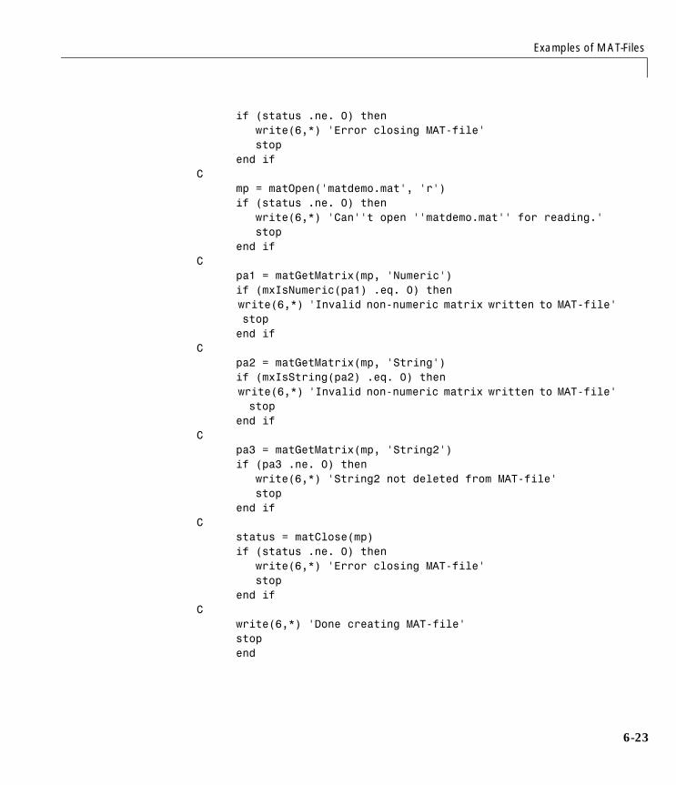
Examples of MAT-Files
6-23
if (status .ne. 0) then write(6,*) 'Error closing MAT-file' stop end ifC mp = matOpen('matdemo.mat', 'r') if (status .ne. 0) then write(6,*) 'Can''t open ''matdemo.mat'' for reading.' stop end ifC pa1 = matGetMatrix(mp, 'Numeric') if (mxIsNumeric(pa1) .eq. 0) then write(6,*) 'Invalid non-numeric matrix written to MAT-file' stop end ifC pa2 = matGetMatrix(mp, 'String') if (mxIsString(pa2) .eq. 0) then write(6,*) 'Invalid non-numeric matrix written to MAT-file' stop end ifC pa3 = matGetMatrix(mp, 'String2') if (pa3 .ne. 0) then write(6,*) 'String2 not deleted from MAT-file' stop end ifC status = matClose(mp) if (status .ne. 0) then write(6,*) 'Error closing MAT-file' stop end ifC write(6,*) 'Done creating MAT-file' stop end
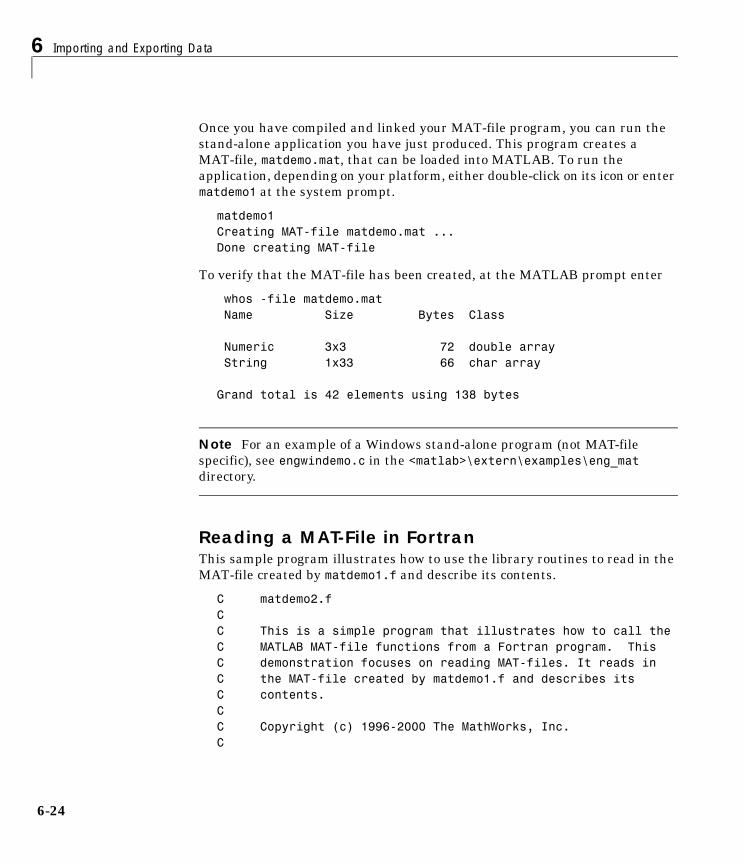
6 Importing and Exporting Data
6-24
Once you have compiled and linked your MAT-file program, you can run the stand-alone application you have just produced. This program creates a MAT-file, matdemo.mat, that can be loaded into MATLAB. To run the application, depending on your platform, either double-click on its icon or enter matdemo1 at the system prompt.
matdemo1Creating MAT-file matdemo.mat ...Done creating MAT-file
To verify that the MAT-file has been created, at the MATLAB prompt enter
whos -file matdemo.mat Name Size Bytes Class Numeric 3x3 72 double array String 1x33 66 char array Grand total is 42 elements using 138 bytes
Note For an example of a Windows stand-alone program (not MAT-file specific), see engwindemo.c in the <matlab>\extern\examples\eng_mat directory.
Reading a MAT-File in FortranThis sample program illustrates how to use the library routines to read in the MAT-file created by matdemo1.f and describe its contents.
C matdemo2.fCC This is a simple program that illustrates how to call theC MATLAB MAT-file functions from a Fortran program. ThisC demonstration focuses on reading MAT-files. It reads inC the MAT-file created by matdemo1.f and describes itsC contents.CC Copyright (c) 1996-2000 The MathWorks, Inc.C

Examples of MAT-Files
6-25
C--------------------------------------------------------------C $Revision: 1.7 $C program matdemo2C--------------------------------------------------------------C (integer) Replace integer by integer*8 on the DEC Alpha C platform.C integer matOpen, matGetDir, matGetNextMatrix integer mp, dir, adir(100), paC--------------------------------------------------------------CC Other variable declarations hereC integer mxGetM, mxGetN, matClose integer ndir, i, stat character*32 names(100), name, mxGetNameCC-------------------------------------------------------------C Open file and read directory.C-------------------------------------------------------------C mp = matOpen('matdemo.mat', 'r') if (mp .eq. 0) then write(6,*) 'Can''t open ''matdemo.mat''.' stop end ifCC Read directory.C dir = matgetdir(mp, ndir) if (dir .eq. 0) then write(6,*) 'Can''t read directory.' stop endifCC Copy integer into an array of pointers.C call mxCopyPtrToPtrArray(dir, adir, ndir)
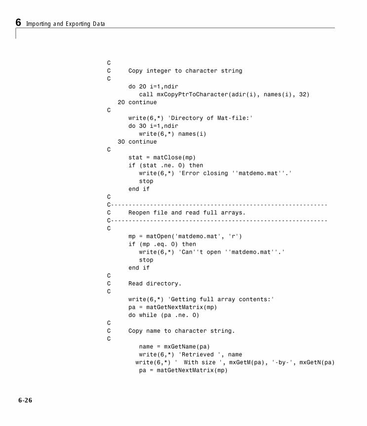
6 Importing and Exporting Data
6-26
CC Copy integer to character stringC do 20 i=1,ndir call mxCopyPtrToCharacter(adir(i), names(i), 32) 20 continueC write(6,*) 'Directory of Mat-file:' do 30 i=1,ndir write(6,*) names(i) 30 continueC stat = matClose(mp) if (stat .ne. 0) then write(6,*) 'Error closing ''matdemo.mat''.' stop end ifCC-------------------------------------------------------------C Reopen file and read full arrays.C-------------------------------------------------------------C mp = matOpen('matdemo.mat', 'r') if (mp .eq. 0) then write(6,*) 'Can''t open ''matdemo.mat''.' stop end ifCC Read directory.C write(6,*) 'Getting full array contents:' pa = matGetNextMatrix(mp) do while (pa .ne. 0)CC Copy name to character string.C name = mxGetName(pa) write(6,*) 'Retrieved ', name write(6,*) ' With size ', mxGetM(pa), '-by-', mxGetN(pa) pa = matGetNextMatrix(mp)
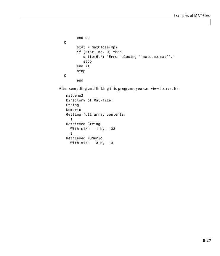
Examples of MAT-Files
6-27
end doC stat = matClose(mp) if (stat .ne. 0) then write(6,*) 'Error closing ''matdemo.mat''.' stop end if stopC end
After compiling and linking this program, you can view its results.
matdemo2 Directory of Mat-file: String Numeric Getting full array contents: 1 Retrieved String With size 1-by- 33 3 Retrieved Numeric With size 3-by- 3
6 Importing and Exporting Data
6-28
Compiling and Linking MAT-File ProgramsThis section describes the steps required to compile and link MAT-file programs on UNIX and Windows systems. It begins by looking at a special consideration for compilers that do not mask floating-point exceptions. Topics covered are:
• “Masking Floating Point Exceptions”
• “Compiling and Linking on UNIX”
• “Compiling and Linking on Windows”
Masking Floating Point ExceptionsCertain mathematical operations can result in nonfinite values. For example, division by zero results in the nonfinite IEEE value, inf. A floating-point exception occurs when such an operation is performed. Because MATLAB uses an IEEE model that supports nonfinite values such as inf and NaN, MATLAB disables, or masks, floating-point exceptions.
Some compilers do not mask floating-point exceptions by default. This causes MAT-file applications built with such compilers to terminate when a floating-point exception occurs. Consequently, you need to take special precautions when using these compilers to mask floating-point exceptions so that your MAT-file application will perform properly.
Note MATLAB-based applications should never get floating-point exceptions. If you do get a floating-point exception, verify that any third party libraries that you link against do not enable floating-point exception handling.
The only compiler and platform on which you need to mask floating-point exceptions is the Borland C++ compiler on Windows.
Borland C++ Compiler on WindowsTo mask floating-point exceptions when using the Borland C++ compiler on the Windows platform, you must add some code to your program. Include the following at the beginning of your main() or WinMain() function, before any calls to MATLAB API functions.

Compiling and Linking MAT-File Programs
6-29
#include <float.h> . . ._control87(MCW_EM,MCW_EM); . . .
Compiling and Linking on UNIXUnder UNIX at runtime, you must tell the system where the API shared libraries reside. These sections provide the necessary UNIX commands depending on your shell and system architecture.
Setting Runtime Library PathIn C shell, the command to set the library path is
setenv LD_LIBRARY_PATH <matlab>/extern/lib/$Arch:$LD_LIBRARY_PATH
In Bourne shell, the commands to set the library path are
LD_LIBRARY_PATH=<matlab>/extern/lib/$Arch:$LD_LIBRARY_PATHexport LD_LIBRARY_PATH
where <matlab> is the MATLAB root directory and $Arch is your system architecture (alpha, glnx86, sgi, sol2, hp700, or ibm_rs).
Note that the environment variable (LD_LIBRARY_PATH in this example) varies on several platforms. The following table lists the different environment variable names you should use on these systems.
It is convenient to place these commands in a startup script such as ~/.cshrc for C shell or ~/.profile for Bourne shell.
Table 6-5: Environment Variable Names
Architecture Environment Variable
HP700 SHLIB_PATH
IBM RS/6000 LIBPATH
6 Importing and Exporting Data
6-30
Using the Options FileMATLAB provides an options file, matopts.sh, that lets you use the mex script to easily compile and link MAT-file applications. For example, to compile and link the matcreat.c example, you can use
mex -f <matlab>/bin/matopts.sh <pathname>/matcreat.c
where <pathname> specifies the complete path to the specified file.
If you need to modify the options file for your particular compiler or platform, use the -v switch to view the current compiler and linker settings and then make the appropriate changes in a local copy of the matopts.sh file.
Compiling and Linking on WindowsTo compile and link Fortran or C MAT-file programs, use the mex script with a MAT options file. Table 1-2, Options Files, on page 1-17 lists the MAT options files included in this release. All of these options files are located in <matlab>\bin\win32\mexopts.
As an example, to compile and link the stand-alone MAT application matcreat.c on Windows using MSVC (Version 5.0), use
mex -f <matlab>\bin\win32\mexopts\msvc50engmatopts.bat <pathname>\matcreat.c
where <pathname> specifies the complete path to the specified file. If you need to modify the options file for your particular compiler, use the -v switch to view the current compiler and linker settings and then make the appropriate changes in a local copy of the options file.
7
ActiveX and DDE Support
Introducing MATLAB ActiveX Integration . . . . . . 7-3ActiveX Concepts and Terminology . . . . . . . . . . . 7-3MATLAB ActiveX Support Overview . . . . . . . . . . 7-4
MATLAB ActiveX Client Support . . . . . . . . . . 7-6Using ActiveX Objects . . . . . . . . . . . . . . . . 7-6
Writing Event Handlers . . . . . . . . . . . . . . . 7-8
Additional ActiveX Client Information . . . . . . . . 7-10Releasing Interfaces . . . . . . . . . . . . . . . . . 7-10Using ActiveX Collections . . . . . . . . . . . . . . . 7-10Converting Data . . . . . . . . . . . . . . . . . . . 7-11Using MATLAB As a DCOM Server Client . . . . . . . . 7-12MATLAB ActiveX Support Limitations . . . . . . . . . . 7-13MATLAB Sample Control . . . . . . . . . . . . . . . 7-13Using MATLAB As an Automation Client . . . . . . . . 7-13
MATLAB ActiveX Automation Server Support . . . . 7-16MATLAB ActiveX Automation Methods . . . . . . . . . 7-17MATLAB ActiveX Automation Properties . . . . . . . . . 7-20
Additional ActiveX Server Information . . . . . . . . 7-21Launching the MATLAB ActiveX Server . . . . . . . . . 7-21Specifying a Shared or Dedicated Server . . . . . . . . . 7-21Using MATLAB As a DCOM Server . . . . . . . . . . . 7-22
Dynamic Data Exchange (DDE) . . . . . . . . . . . 7-23DDE Concepts and Terminology . . . . . . . . . . . . 7-23Accessing MATLAB As a Server . . . . . . . . . . . . 7-25The DDE Name Hierarchy . . . . . . . . . . . . . . . 7-26Example: Using Visual Basic and the MATLAB DDE Server . 7-29Using MATLAB As a Client . . . . . . . . . . . . . . 7-31DDE Advisory Links . . . . . . . . . . . . . . . . . 7-32
7 ActiveX and DDE Support
7-2
ActiveX is a set of object-oriented technologies and tools that allow software developers to integrate application-specific components from different vendors into their own application solution. ActiveX Control components can be both visually and programmatically integrated into an ActiveX control container, such as a MATLAB figure window. ActiveX Automation allows MATLAB to both control and be controlled by other ActiveX components.
Dynamic Data Exchange, or DDE, is a feature of Windows that allows two programs to share data or send commands directly to each other. MATLAB provides functions that use this data exchange to enable access between MATLAB and other Windows applications in a wide range of contexts.
This chapter discusses the following topics:
• “Introducing MATLAB ActiveX Integration”
• “MATLAB ActiveX Client Support”
• “Writing Event Handlers”
• “Additional ActiveX Client Information”
• “MATLAB ActiveX Automation Server Support”
• “Additional ActiveX Server Information”
• “Dynamic Data Exchange (DDE)”
Introducing MATLAB ActiveX Integration
7-3
Introducing MATLAB ActiveX Integration ActiveX is a Microsoft Windows protocol for component integration. Using ActiveX, developers and end users can select application-specific, ActiveX components produced by different vendors and seamlessly integrate them into a complete application solution. For example, a single application may require database access, mathematical analysis, and presentation quality business graphs. Using ActiveX, a developer may choose a database access component by one vendor, a business graph component by another, and integrate these into a mathematical analysis package produced by yet a third.
ActiveX Concepts and Terminology
COMActiveX is a family of related object-oriented technologies that have a common root, called the Component Object Model, or COM. Each object-oriented language or environment has an object model that defines certain characteristics of objects in that environment, such as how objects are located, instantiated, or identified. COM defines the object model for all ActiveX objects.
ActiveX InterfacesEach ActiveX object supports one or more named interfaces. An interface is a logically related collection of methods, properties, and events. Methods are similar to function calls in that they are a request for the object to perform some action. Properties are state variables maintained by the object, such as the color of text, or the name of a file on which the control is acting. Events are notifications that the control forwards back to its client (similar to Handle Graphics® callbacks.)
For example, the sample control shipped with MATLAB has the following methods, properties, and events:
• MethodsRedraw - causes the control to redrawBeep - causes the control to beepAboutBox - display the control’s “About” dialog
7 ActiveX and DDE Support
7-4
• PropertiesRadius (integer) - sets the radius of the circle drawn by the controlLabel (string) - text to be drawn in the control
• Events
Click - fired when the user clicks on the control
One important characteristic of COM is that it defines an object model in which objects support multiple interfaces. Some interfaces are standard interfaces, which are defined by Microsoft and are part of ActiveX, and some interfaces are custom interfaces, which are defined by individual component vendors. In order to use any ActiveX object, you must learn about which custom interfaces it supports, and the interface’s methods, properties, and events. The ActiveX object’s vendor provides this information.
MATLAB ActiveX Support OverviewMATLAB supports two ActiveX technologies: ActiveX control containment and ActiveX Automation. ActiveX controls are application components that can be both visually and programmatically integrated into an ActiveX control container, such as MATLAB figure windows. Some examples of useful ActiveX controls are the Microsoft Internet Explorer Web Browser control, the Microsoft Windows Communications control for serial port access, and the graphical user interface controls delivered with the Visual Basic development environment.
ActiveX Automation allows MATLAB to both control and be controlled by other ActiveX components. When MATLAB is controlled by another component, it is acting as an automation server. When MATLAB controls another component, MATLAB is the automation client, and the other component is the automation server.
MATLAB automation server capabilities include the ability to execute commands in the MATLAB workspace, and to get and put matrices directly from and into the workspace. MATLAB automation client capabilities allow MATLAB, through M-code, to programmatically instantiate and manipulate automation servers. The MATLAB automation client capabilities are a subset of the MATLAB control containment support, since you use the automation client capabilities to manipulate controls as well as automation servers. In other words, all ActiveX controls are ActiveX automation servers, but not all automation servers are necessarily controls.
Introducing MATLAB ActiveX Integration
7-5
In general, servers that are not controls will not be physically or visually embedded in the client application. (MATLAB is a good example — MATLAB is not itself a control, but it is a server. So, MATLAB cannot be physically embedded within another client. However, since MATLAB is a control container, other ActiveX controls can be embedded within MATLAB.)
In addition, MATLAB ships with a very simple sample ActiveX control that draws a circle on the screen and displays some text. This allows MATLAB users to try out MATLAB’s ActiveX control support with a known control. For more information, see “MATLAB Sample Control” on page 7-13.
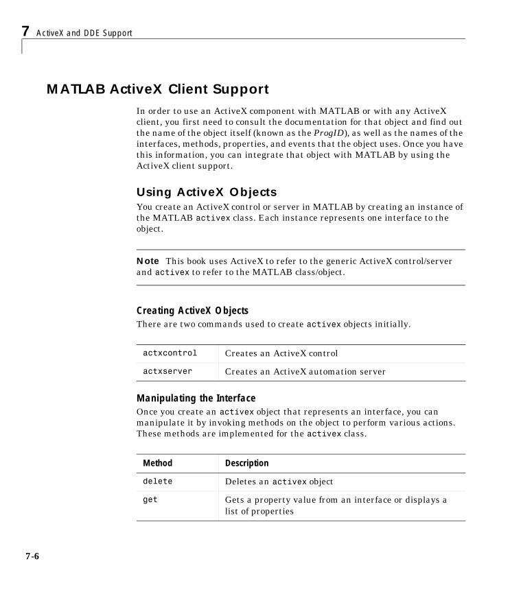
7 ActiveX and DDE Support
7-6
MATLAB ActiveX Client SupportIn order to use an ActiveX component with MATLAB or with any ActiveX client, you first need to consult the documentation for that object and find out the name of the object itself (known as the ProgID), as well as the names of the interfaces, methods, properties, and events that the object uses. Once you have this information, you can integrate that object with MATLAB by using the ActiveX client support.
Using ActiveX ObjectsYou create an ActiveX control or server in MATLAB by creating an instance of the MATLAB activex class. Each instance represents one interface to the object.
Note This book uses ActiveX to refer to the generic ActiveX control/server and activex to refer to the MATLAB class/object.
Creating ActiveX ObjectsThere are two commands used to create activex objects initially.
Manipulating the InterfaceOnce you create an activex object that represents an interface, you can manipulate it by invoking methods on the object to perform various actions. These methods are implemented for the activex class.
actxcontrol Creates an ActiveX control
actxserver Creates an ActiveX automation server
Method Description
delete Deletes an activex object
get Gets a property value from an interface or displays a list of properties
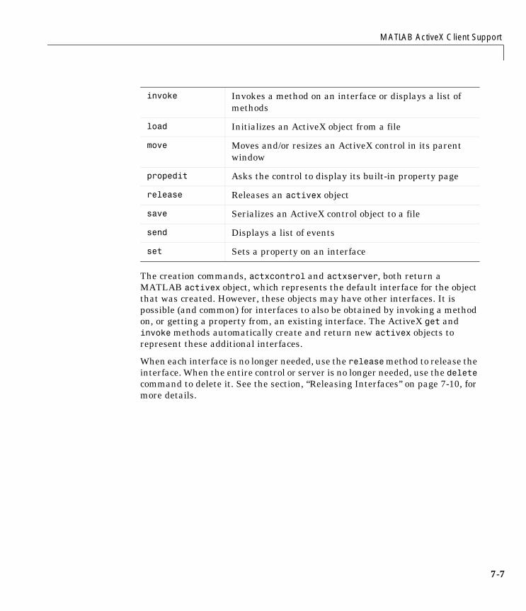
MATLAB ActiveX Client Support
7-7
The creation commands, actxcontrol and actxserver, both return a MATLAB activex object, which represents the default interface for the object that was created. However, these objects may have other interfaces. It is possible (and common) for interfaces to also be obtained by invoking a method on, or getting a property from, an existing interface. The ActiveX get and invoke methods automatically create and return new activex objects to represent these additional interfaces.
When each interface is no longer needed, use the release method to release the interface. When the entire control or server is no longer needed, use the delete command to delete it. See the section, “Releasing Interfaces” on page 7-10, for more details.
invoke Invokes a method on an interface or displays a list of methods
load Initializes an ActiveX object from a file
move Moves and/or resizes an ActiveX control in its parent window
propedit Asks the control to display its built-in property page
release Releases an activex object
save Serializes an ActiveX control object to a file
send Displays a list of events
set Sets a property on an interface
7 ActiveX and DDE Support
7-8
Writing Event HandlersActiveX events are invoked when a control wants to notify its container that something of interest has occurred. For example, many controls trigger an event when the user single-clicks on the control. In MATLAB, when a control is created, you may optionally supply a callback (also known as an event handler function) as the last argument to the actxcontrol command or a cell array that contains the event handlers.
h = actxcontrol (progid [, position [, handle ...[, callback | {event1 eventhandler1; event2 eventhandler2; …}]]])
The event handler function (callback) is called whenever the control triggers any event. The event handler function must be an M-function that accepts a variable number of arguments of the following form:
function event (varargin)if (str2num(vararg{1}) == -600) disp ('Click Event Fired');end
All arguments passed to this function are MATLAB strings. The first argument to the event handler is a string that represents the number of the event that caused the event handler to be called. The remaining arguments are the values passed by the control with the event. These values will vary with the particular event and control being used. The list of events that control invocations and their corresponding event numbers and parameters must be obtained from the control’s documentation. In order to use events with MATLAB, you will need to find out the numerical values that the control uses for each event so that you can use these in the event handler.
The event handlers that are used in the cell array style are slightly different than those used in the callback style. The first argument in the cell array style is a reference to the object itself. The second argument is the event number, which, unlike the callback style, is not a string that represents the number. (Subsequent arguments vary depending on the event.)
These sample event handlers, myclick.m, my2click.m, and mymoused.m correspond to the actxcontrol example.
Writing Event Handlers
7-9
function myclick(varargin)disp('Single click function')
function my2click(varargin)disp('Double click function')
function mymoused(varargin)disp('You have reached the mouse down function')disp('The X position is: ')varargin(5)disp('The Y position is: ')varargin(6)
You can use the same event handler for all the events you want to monitor using the cell array pairs. Response time will be better than using the callback style.
For instance
h = actxcontrol('SELECTOR.SelectorCtrl.1', [0 0 200 200], f, ...{'Click' 'allevents'; 'DblClick' 'allevents'; ...'MouseDown' 'allevents'})
and allevents.m is
function allevents(varargin)if (varargin{2} = -600)
disp ('Single Click Event Fired')elseif (varargin{2} = -601)
disp ('Double Click Event Fired')elseif (varargin{2} = -605)
disp ('Mousedown Event Fired')end
Note MATLAB does not support event arguments passed by reference or return values from events.
7 ActiveX and DDE Support
7-10
Additional ActiveX Client Information
Releasing InterfacesEach ActiveX object can support one or more interfaces. In MATLAB, an interface is represented by an instance of the activex class. There are three ways to get a valid interface object into the MATLAB workspace:
• Return value from actxcontrol/actxserver
• Return value from a property via get
• Return value from a method invocation via invoke
In each case, once the interface is represented by an activex object in the workspace, it must be released when you are finished using it. Failure to release interface handles results in memory and resources being consumed. Alternatively, you can use the delete command on any valid interface object, and all interfaces for that object are automatically released, and thus invalidated, and the ActiveX server or control itself is deleted.
MATLAB automatically releases all interfaces for an ActiveX control when the figure window that contains that control is deleted or closed. MATLAB also automatically releases all handles for an ActiveX automation server when MATLAB is shut down.
Using ActiveX CollectionsActiveX collections are a way to support groups of related ActiveX objects that can be iterated over. A collection is itself a special interface with a Count property (read only), which contains the number of items in the collection, and an Item method, which allows you to retrieve a single item from the collection.
The Item method is indexed, which means that it requires an argument that specifies which item in the collection is being requested. The data type of the index can be any data type that is appropriate for the particular collection and is specific to the control or server that supports the collection. Although integer indices are common, the index could just as easily be a string value. Often, the return value from the Item method is itself an interface. Like all interfaces, this interface should be released when you are finished with it.
This example iterates through the members of a collection. Each member of the collection is itself an interface (called Plot and represented by a MATLAB
Additional ActiveX Client Information
7-11
activex object called hPlot.) In particular, this example iterates through a collection of Plot interfaces, invokes the Redraw method for each interface, and then releases each interface.
hCollection = get (hControl, 'Plots');for i=1:get (hCollection, 'Count')hPlot = invoke (hCollection, 'Item', i);
invoke (hPlot, 'Redraw');release (hPlot);
end;release (hCollection);
Converting DataSince ActiveX defines a number of different data formats and types, you will need to know how MATLAB converts data from activex objects into variables in the MATLAB workspace. Data from activex objects must be converted:
• When a property value is retrieved
• When a value is returned from a method invocation
This chart shows how ActiveX data types are converted into variables in the MATLAB workspace.
ActiveX Data Type MATLAB Variable
StringFile TimeErrorDecimal Date
MATLAB String
CurrencyHresultInt/Unsigned (2, 4, 8)Bool
Scalar Double
Real (Single/Double
Null NaN
Precision)
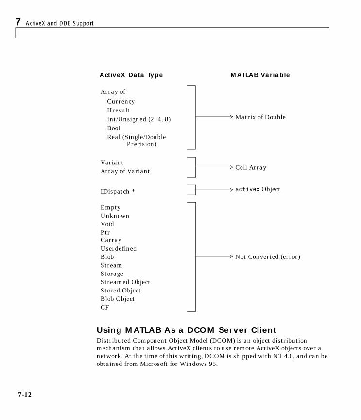
7 ActiveX and DDE Support
7-12
Using MATLAB As a DCOM Server ClientDistributed Component Object Model (DCOM) is an object distribution mechanism that allows ActiveX clients to use remote ActiveX objects over a network. At the time of this writing, DCOM is shipped with NT 4.0, and can be obtained from Microsoft for Windows 95.
ActiveX Data Type MATLAB Variable
EmptyUnknownVoid
Carray
Not Converted (error)UserdefinedBlobStreamStorageStreamed ObjectStored ObjectBlob ObjectCF
VariantCell ArrayArray of Variant
IDispatch * activex Object
CurrencyHresultInt/Unsigned (2, 4, 8)Bool
Matrix of Double
Real (Single/Double
Array of
Ptr
Precision)
Additional ActiveX Client Information
7-13
MATLAB has been tested as a DCOM server with Windows NT 4.0 only. Additionally, MATLAB can be used as a DCOM client with remote automation servers if the operating system on which MATLAB is running is DCOM enabled.
Note If you use MATLAB as a remote DCOM server, all MATLAB windows will appear on the remote machine.
MATLAB ActiveX Support LimitationsThe following is a list of limitations of MATLAB ActiveX support:
• MATLAB only supports indexed collections.
• ActiveX controls are not printed with figure windows.
• MATLAB does not support event arguments passed by reference.
• MATLAB does not support returning values from event handler functions.
• The position vector of a control cannot be changed or queried.
• MATLAB does not support method or event arguments passed by reference.
MATLAB Sample ControlMATLAB ships with a very simple example ActiveX control that draws a circle on the screen, displays some text, and fires a clicked event when the user clicks on the control. This control makes it easy to try out ActiveX control support with a known control. The control can be created by running the mwsamp file in the winfun directory.
The control is stored in the MATLAB bin, or executable, directory along with the control’s type library. The type library is a binary file used by ActiveX tools to decipher the control’s capabilities.
Using MATLAB As an Automation ClientThis example uses MATLAB as an automation client and Microsoft Excel as the server. It provides a good overview of typical functions. In addition, it is a good example of using the automation interface of another application.
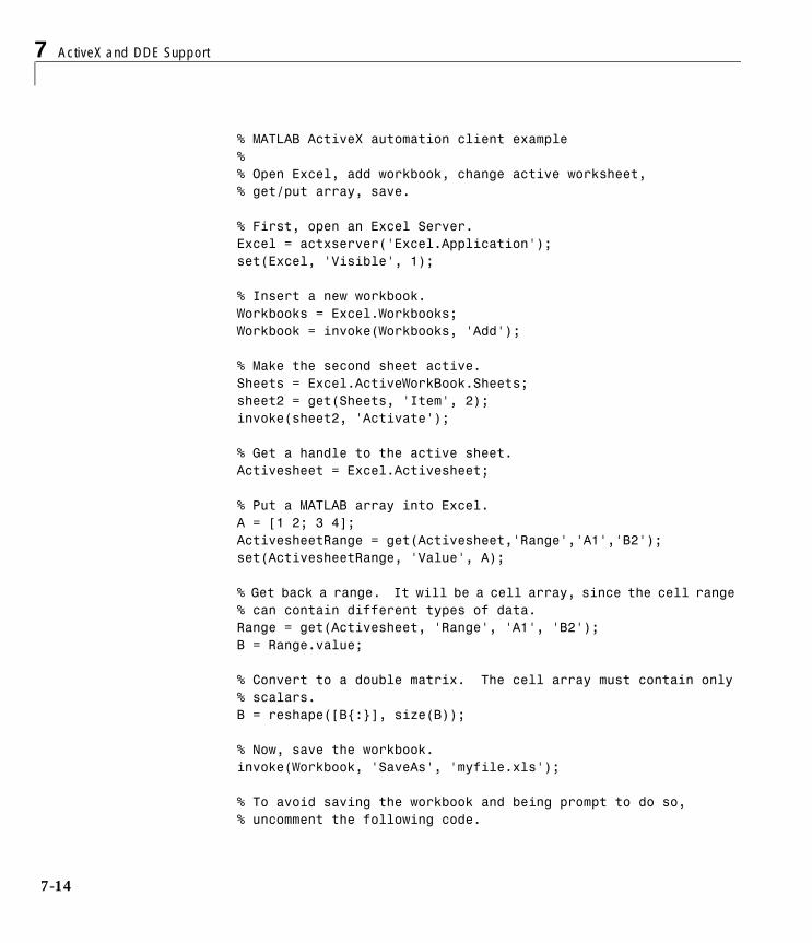
7 ActiveX and DDE Support
7-14
% MATLAB ActiveX automation client example %% Open Excel, add workbook, change active worksheet, % get/put array, save.
% First, open an Excel Server.Excel = actxserver('Excel.Application');set(Excel, 'Visible', 1);
% Insert a new workbook.Workbooks = Excel.Workbooks;Workbook = invoke(Workbooks, 'Add');
% Make the second sheet active.Sheets = Excel.ActiveWorkBook.Sheets;sheet2 = get(Sheets, 'Item', 2);invoke(sheet2, 'Activate');
% Get a handle to the active sheet.Activesheet = Excel.Activesheet;
% Put a MATLAB array into Excel.A = [1 2; 3 4]; ActivesheetRange = get(Activesheet,'Range','A1','B2');set(ActivesheetRange, 'Value', A);
% Get back a range. It will be a cell array, since the cell range % can contain different types of data.Range = get(Activesheet, 'Range', 'A1', 'B2');B = Range.value;
% Convert to a double matrix. The cell array must contain only% scalars.B = reshape([B{:}], size(B));
% Now, save the workbook.invoke(Workbook, 'SaveAs', 'myfile.xls');
% To avoid saving the workbook and being prompt to do so,% uncomment the following code.
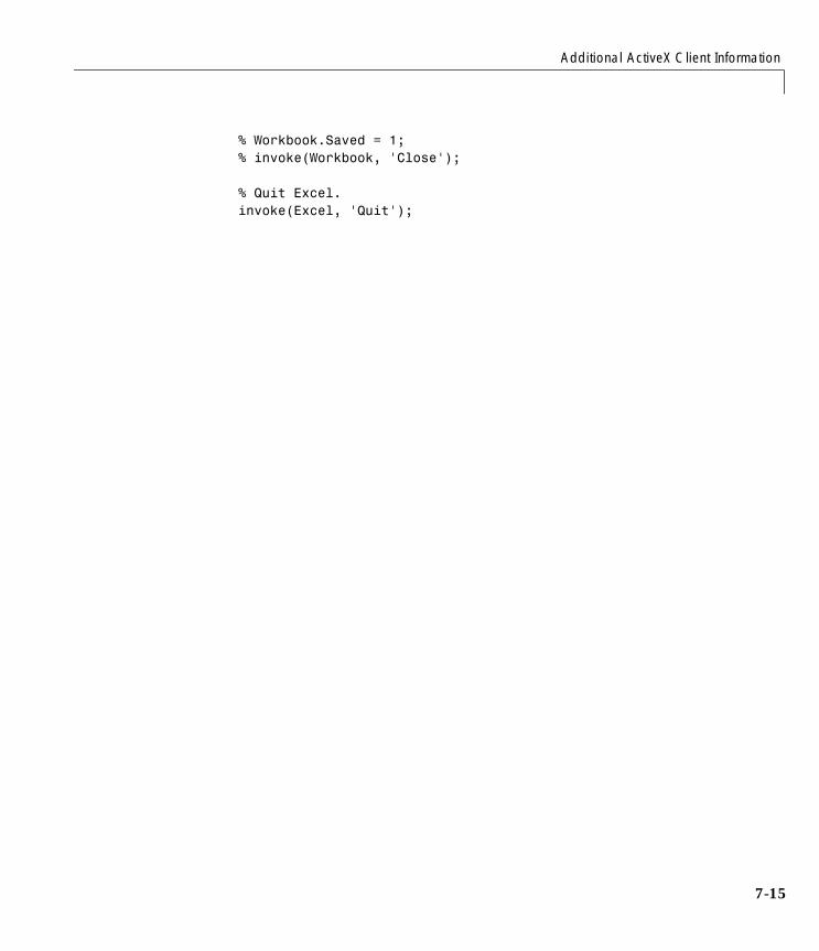
Additional ActiveX Client Information
7-15
% Workbook.Saved = 1;% invoke(Workbook, 'Close');
% Quit Excel.invoke(Excel, 'Quit');
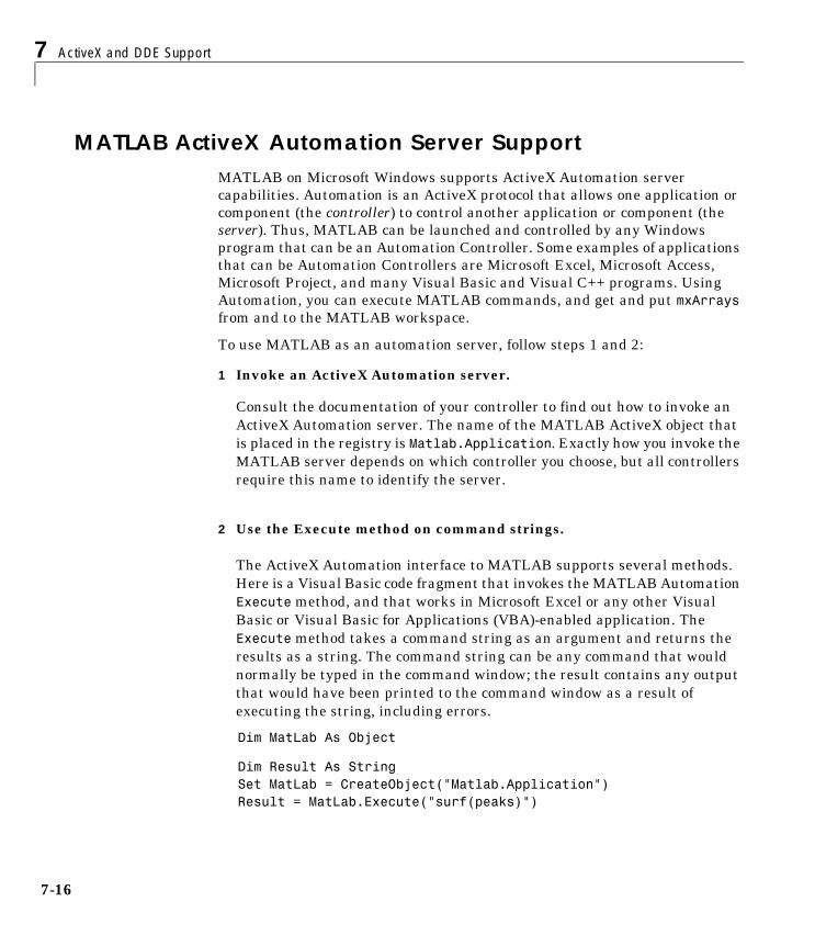
7 ActiveX and DDE Support
7-16
MATLAB ActiveX Automation Server SupportMATLAB on Microsoft Windows supports ActiveX Automation server capabilities. Automation is an ActiveX protocol that allows one application or component (the controller) to control another application or component (the server). Thus, MATLAB can be launched and controlled by any Windows program that can be an Automation Controller. Some examples of applications that can be Automation Controllers are Microsoft Excel, Microsoft Access, Microsoft Project, and many Visual Basic and Visual C++ programs. Using Automation, you can execute MATLAB commands, and get and put mxArrays from and to the MATLAB workspace.
To use MATLAB as an automation server, follow steps 1 and 2:
1 Invoke an ActiveX Automation server.
Consult the documentation of your controller to find out how to invoke an ActiveX Automation server. The name of the MATLAB ActiveX object that is placed in the registry is Matlab.Application. Exactly how you invoke the MATLAB server depends on which controller you choose, but all controllers require this name to identify the server.
2 Use the Execute method on command strings.
The ActiveX Automation interface to MATLAB supports several methods. Here is a Visual Basic code fragment that invokes the MATLAB Automation Execute method, and that works in Microsoft Excel or any other Visual Basic or Visual Basic for Applications (VBA)-enabled application. The Execute method takes a command string as an argument and returns the results as a string. The command string can be any command that would normally be typed in the command window; the result contains any output that would have been printed to the command window as a result of executing the string, including errors.
Dim MatLab As Object
Dim Result As StringSet MatLab = CreateObject("Matlab.Application")Result = MatLab.Execute("surf(peaks)")
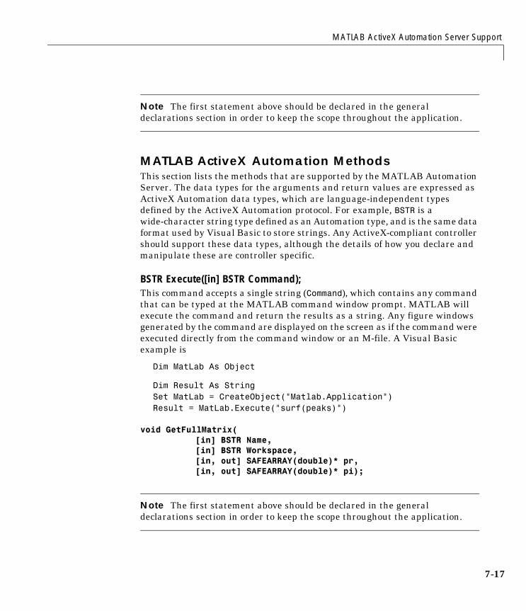
MATLAB ActiveX Automation Server Support
7-17
Note The first statement above should be declared in the general declarations section in order to keep the scope throughout the application.
MATLAB ActiveX Automation MethodsThis section lists the methods that are supported by the MATLAB Automation Server. The data types for the arguments and return values are expressed as ActiveX Automation data types, which are language-independent types defined by the ActiveX Automation protocol. For example, BSTR is a wide-character string type defined as an Automation type, and is the same data format used by Visual Basic to store strings. Any ActiveX-compliant controller should support these data types, although the details of how you declare and manipulate these are controller specific.
BSTR Execute([in] BSTR Command);This command accepts a single string (Command), which contains any command that can be typed at the MATLAB command window prompt. MATLAB will execute the command and return the results as a string. Any figure windows generated by the command are displayed on the screen as if the command were executed directly from the command window or an M-file. A Visual Basic example is
Dim MatLab As Object
Dim Result As StringSet MatLab = CreateObject("Matlab.Application")Result = MatLab.Execute("surf(peaks)")
void GetFullMatrix([in] BSTR Name,[in] BSTR Workspace,[in, out] SAFEARRAY(double)* pr, [in, out] SAFEARRAY(double)* pi);
Note The first statement above should be declared in the general declarations section in order to keep the scope throughout the application.
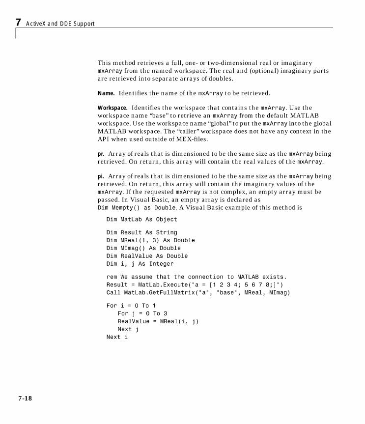
7 ActiveX and DDE Support
7-18
This method retrieves a full, one- or two-dimensional real or imaginary mxArray from the named workspace. The real and (optional) imaginary parts are retrieved into separate arrays of doubles.
Name. Identifies the name of the mxArray to be retrieved.
Workspace. Identifies the workspace that contains the mxArray. Use the workspace name “base” to retrieve an mxArray from the default MATLAB workspace. Use the workspace name “global” to put the mxArray into the global MATLAB workspace. The “caller” workspace does not have any context in the API when used outside of MEX-files.
pr. Array of reals that is dimensioned to be the same size as the mxArray being retrieved. On return, this array will contain the real values of the mxArray.
pi. Array of reals that is dimensioned to be the same size as the mxArray being retrieved. On return, this array will contain the imaginary values of the mxArray. If the requested mxArray is not complex, an empty array must be passed. In Visual Basic, an empty array is declared as Dim Mempty() as Double. A Visual Basic example of this method is
Dim MatLab As Object
Dim Result As StringDim MReal(1, 3) As DoubleDim MImag() As DoubleDim RealValue As DoubleDim i, j As Integer
rem We assume that the connection to MATLAB exists.Result = MatLab.Execute("a = [1 2 3 4; 5 6 7 8;]")Call MatLab.GetFullMatrix("a", "base", MReal, MImag)
For i = 0 To 1For j = 0 To 3RealValue = MReal(i, j) Next j
Next i
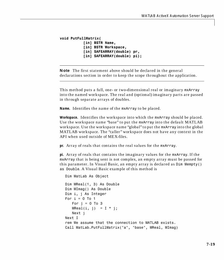
MATLAB ActiveX Automation Server Support
7-19
void PutFullMatrix([in] BSTR Name, [in] BSTR Workspace, [in] SAFEARRAY(double) pr, [in] SAFEARRAY(double) pi);
Note The first statement above should be declared in the general declarations section in order to keep the scope throughout the application.
This method puts a full, one- or two-dimensional real or imaginary mxArray into the named workspace. The real and (optional) imaginary parts are passed in through separate arrays of doubles.
Name. Identifies the name of the mxArray to be placed.
Workspace. Identifies the workspace into which the mxArray should be placed. Use the workspace name “base” to put the mxArray into the default MATLAB workspace. Use the workspace name “global” to put the mxArray into the global MATLAB workspace. The “caller” workspace does not have any context in the API when used outside of MEX-files.
pr. Array of reals that contains the real values for the mxArray.
pi. Array of reals that contains the imaginary values for the mxArray. If the mxArray that is being sent is not complex, an empty array must be passed for this parameter. In Visual Basic, an empty array is declared as Dim Mempty() as Double. A Visual Basic example of this method is
Dim MatLab As Object
Dim MReal(1, 3) As DoubleDim MImag() As DoubleDim i, j As IntegerFor i = 0 To 1
For j = 0 To 3MReal(i, j) = I * j;Next j
Next Irem We assume that the connection to MATLAB exists.Call MatLab.PutFullMatrix("a", "base", MReal, MImag)
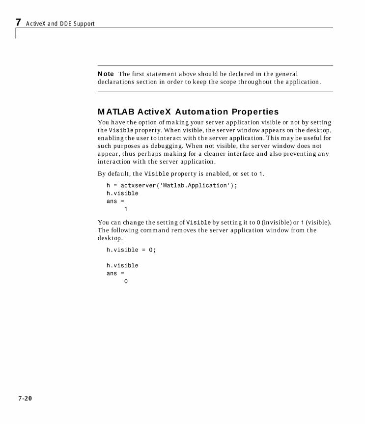
7 ActiveX and DDE Support
7-20
Note The first statement above should be declared in the general declarations section in order to keep the scope throughout the application.
MATLAB ActiveX Automation PropertiesYou have the option of making your server application visible or not by setting the Visible property. When visible, the server window appears on the desktop, enabling the user to interact with the server application. This may be useful for such purposes as debugging. When not visible, the server window does not appear, thus perhaps making for a cleaner interface and also preventing any interaction with the server application.
By default, the Visible property is enabled, or set to 1.
h = actxserver('Matlab.Application');h.visibleans = 1
You can change the setting of Visible by setting it to 0 (invisible) or 1 (visible). The following command removes the server application window from the desktop.
h.visible = 0;
h.visibleans = 0

Additional ActiveX Server Information
7-21
Additional ActiveX Server Information
Launching the MATLAB ActiveX ServerFor MATLAB to act as an automation server, it must be started with the /Automation command line argument. Microsoft Windows does this automatically when an ActiveX connection is established by a controller. However, if MATLAB is already running and was launched without this parameter, any request by an automation controller to connect to MATLAB as a server will cause Windows to launch another instance of MATLAB with the /Automation parameter. This protects controllers from interfering with any interactive MATLAB sessions that may be running.
Specifying a Shared or Dedicated ServerYou can launch the MATLAB Automation server in one of two modes — shared or dedicated. A dedicated server is dedicated to a single client; a shared server is shared by multiple clients.
The mode is determined by the Program ID (ProgID) used by the client to launch MATLAB. The ProgID, Matlab.Application, (or the version-specific ProgID, Matlab.Application.5) specifies the default mode, which is shared. To specify a dedicated server, use the ProgID, Matlab.Application.Single, (or the version-specific ProgID, Matlab.Application.Single.5). The term Single refers to the number of clients that may connect to this server.
Once MATLAB is launched as a shared server, all clients that request a connection to MATLAB by using the shared server ProgID will connect to the already running instance of MATLAB. In other words, there is never more than one instance of a shared server running, since it is shared by all clients that use the ProgID that specifies a shared server.
Note Clients will not connect to an interactive instance of MATLAB, that is, an instance of MATLAB that was launched manually and without the /Automation command line flag.
Each client that requests a connection to MATLAB using a dedicated ProgID will cause a separate instance of MATLAB to be launched, and that server will not be shared with any other client. Therefore, there can be several instances
7 ActiveX and DDE Support
7-22
of a dedicated server running simultaneously, since the dedicated server is not shared by multiple clients.
Using MATLAB As a DCOM ServerDCOM is a protocol that allows ActiveX connections to be established over a network. If you are using a version of Windows that supports DCOM (Windows NT 4.0 at the time of this writing) and a controller that supports DCOM, you can use the controller to launch MATLAB on a remote machine. To do this, DCOM must be configured properly, and MATLAB must be installed on each machine that is used as a client or server. (Even though the client machine will not be running MATLAB in such a configuration, the client machine must have a MATLAB installation because certain MATLAB components are required to establish the remote connection.) Consult the DCOM documentation for how to configure DCOM for your environment.
Dynamic Data Exchange (DDE)
7-23
Dynamic Data Exchange (DDE)MATLAB provides functions that enable MATLAB to access other Windows applications and for other Windows applications to access MATLAB in a wide range of contexts. These functions use dynamic data exchange (DDE), software that allows Microsoft Windows applications to communicate with each other by exchanging data.
This section describes using DDE in MATLAB:
• “DDE Concepts and Terminology”
• “Accessing MATLAB As a Server”
• “Using MATLAB As a Client”
• “DDE Advisory Links”
DDE Concepts and TerminologyApplications communicate with each other by establishing a DDE conversation. The application that initiates the conversation is called the client. The application that responds to the client application is called the server.
When a client application initiates a DDE conversation, it must identify two DDE parameters that are defined by the server:
• The name of the application it intends to have the conversation with, called the service name
• The subject of the conversation, called the topic
When a server application receives a request for a conversation involving a supported topic, it acknowledges the request, establishing a DDE conversation. The combination of a service and a topic identifies a conversation uniquely. The service or topic cannot be changed for the duration of the conversation, although the service can maintain more than one conversation.
During a DDE conversation, the client and server applications exchange data concerning items. An item is a reference to data that is meaningful to both applications in a conversation. Either application can change the item during a conversation. These concepts are discussed in more detail below.
7 ActiveX and DDE Support
7-24
The Service NameEvery application that can be a DDE server has a unique service name. The service name is usually the application’s executable filename without any extension. Service names are not case sensitive. Here are some commonly used service names:
• The service name for MATLAB is Matlab.
• The service name for Microsoft Word for Windows is WinWord.
• The service name for Microsoft Excel is Excel.
For the service names of other Windows applications, refer to the application documentation.
The TopicThe topic defines the subject of a DDE conversation and is usually meaningful to both the client and server applications. Topic names are not case sensitive. MATLAB topics are System and Engine and are discussed in “Accessing MATLAB As a Server” on page 7-25. Most applications support the System topic and at least one other topic. Consult your application documentation for information about supported topics.
The ItemEach topic supports one or more items. An item identifies the data being passed during the DDE conversation. Case sensitivity of items depends on the application. MATLAB Engine items are case sensitive if they refer to matrices because matrix names are case sensitive.
Clipboard FormatsDDE uses the Windows clipboard formats for formatting data sent between applications. As a client, MATLAB supports only Text format. As a server, MATLAB supports Text, Metafilepict, and XLTable formats, described below:
• Text – Data in Text format is a buffer of characters terminated by the null character. Lines of text in the buffer are delimited by a carriage return line-feed combination. If the buffer contains columns of data, those columns are delimited by the tab character. MATLAB supports Text format for obtaining the results of a remote EvalString command and requests for matrix data. Also, matrix data can be sent to MATLAB in Text format.
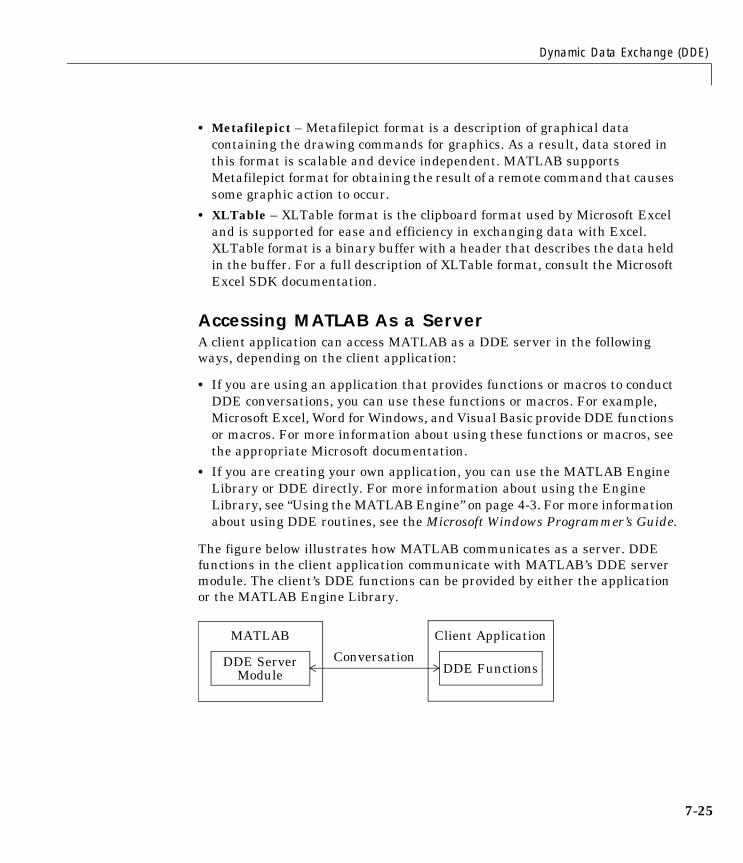
Dynamic Data Exchange (DDE)
7-25
• Metafilepict – Metafilepict format is a description of graphical data containing the drawing commands for graphics. As a result, data stored in this format is scalable and device independent. MATLAB supports Metafilepict format for obtaining the result of a remote command that causes some graphic action to occur.
• XLTable – XLTable format is the clipboard format used by Microsoft Excel and is supported for ease and efficiency in exchanging data with Excel. XLTable format is a binary buffer with a header that describes the data held in the buffer. For a full description of XLTable format, consult the Microsoft Excel SDK documentation.
Accessing MATLAB As a ServerA client application can access MATLAB as a DDE server in the following ways, depending on the client application:
• If you are using an application that provides functions or macros to conduct DDE conversations, you can use these functions or macros. For example, Microsoft Excel, Word for Windows, and Visual Basic provide DDE functions or macros. For more information about using these functions or macros, see the appropriate Microsoft documentation.
• If you are creating your own application, you can use the MATLAB Engine Library or DDE directly. For more information about using the Engine Library, see “Using the MATLAB Engine” on page 4-3. For more information about using DDE routines, see the Microsoft Windows Programmer’s Guide.
The figure below illustrates how MATLAB communicates as a server. DDE functions in the client application communicate with MATLAB’s DDE server module. The client’s DDE functions can be provided by either the application or the MATLAB Engine Library.
MATLAB
DDE ServerModule
Client Application
DDE FunctionsConversation

7 ActiveX and DDE Support
7-26
The DDE Name HierarchyWhen you access MATLAB as a server, you must specify its service name, topic, and item. The figure below illustrates the MATLAB DDE name hierarchy. Topics and items are described in more detail below.
The two MATLAB topics are System and Engine.
MATLAB System TopicThe System topic allows users to browse the list of topics provided by the server, the list of System topic items provided by the server, and the formats supported by the server.
The MATLAB System topic supports these items:
• SysItems
Provides a tab-delimited list of items supported under the System topic (this list).
MATLAB
System
Engine
SysItems
Format
Topics
EngEvalString
EngStringResult
EngFigureResult
<matrix name>
service
topics
items
Dynamic Data Exchange (DDE)
7-27
• Format
Provides a tab-delimited list of string names of all the formats supported by the server. MATLAB supports Text, Metafilepict, and XLTable. These formats are described in “Clipboard Formats” on page 7-24.
• Topics
Provides a tab-delimited list of the names of the topics supported by MATLAB.
MATLAB Engine TopicThe Engine topic allows users to use MATLAB as a server by passing it a command to execute, requesting data, or sending data.
The MATLAB Engine topic supports these items:
• EngEvalString
Specifies an item name, if required, when you send a command to MATLAB for evaluation.
• EngStringResult
Provides the string result of a DDE execute command when you request data from MATLAB.
• EngFigureResult
Provides the graphical result of a DDE execute command when you request data from MATLAB.
• <matrix name>
When requesting data from MATLAB, this is the name of the matrix for which data is being requested. When sending data to MATLAB, this is the name of the matrix to be created or updated.
The MATLAB Engine topic supports three operations that may be used by applications with a DDE client interface. These operations include sending commands to MATLAB for evaluation, requesting data from MATLAB, and sending data to MATLAB.
Sending Commands to MATLAB for EvaluationClients send commands to MATLAB using the DDE execute operation. The Engine topic supports DDE execute in two forms because some clients require that you specify the item name and the command to execute, while others
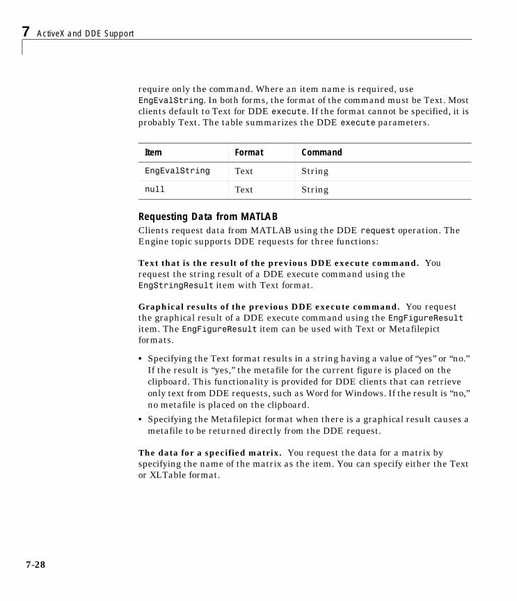
7 ActiveX and DDE Support
7-28
require only the command. Where an item name is required, use EngEvalString. In both forms, the format of the command must be Text. Most clients default to Text for DDE execute. If the format cannot be specified, it is probably Text. The table summarizes the DDE execute parameters.
Requesting Data from MATLABClients request data from MATLAB using the DDE request operation. The Engine topic supports DDE requests for three functions:
Text that is the result of the previous DDE execute command. You request the string result of a DDE execute command using the EngStringResult item with Text format.
Graphical results of the previous DDE execute command. You request the graphical result of a DDE execute command using the EngFigureResult item. The EngFigureResult item can be used with Text or Metafilepict formats.
• Specifying the Text format results in a string having a value of “yes” or “no.” If the result is “yes,” the metafile for the current figure is placed on the clipboard. This functionality is provided for DDE clients that can retrieve only text from DDE requests, such as Word for Windows. If the result is “no,” no metafile is placed on the clipboard.
• Specifying the Metafilepict format when there is a graphical result causes a metafile to be returned directly from the DDE request.
The data for a specified matrix. You request the data for a matrix by specifying the name of the matrix as the item. You can specify either the Text or XLTable format.
Item Format Command
EngEvalString Text String
null Text String
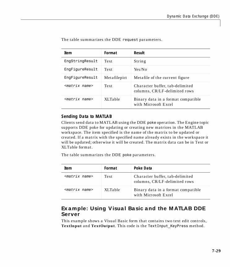
Dynamic Data Exchange (DDE)
7-29
The table summarizes the DDE request parameters.
Sending Data to MATLABClients send data to MATLAB using the DDE poke operation. The Engine topic supports DDE poke for updating or creating new matrices in the MATLAB workspace. The item specified is the name of the matrix to be updated or created. If a matrix with the specified name already exists in the workspace it will be updated; otherwise it will be created. The matrix data can be in Text or XLTable format.
The table summarizes the DDE poke parameters.
Example: Using Visual Basic and the MATLAB DDE ServerThis example shows a Visual Basic form that contains two text edit controls, TextInput and TextOutput. This code is the TextInput_KeyPress method.
Item Format Result
EngStringResult Text String
EngFigureResult Text Yes/No
EngFigureResult Metafilepict Metafile of the current figure
<matrix name> Text Character buffer, tab-delimited columns, CR/LF-delimited rows
<matrix name> XLTable Binary data in a format compatible with Microsoft Excel
Item Format Poke Data
<matrix name> Text Character buffer, tab-delimited columns, CR/LF-delimited rows
<matrix name> XLTable Binary data in a format compatible with Microsoft Excel
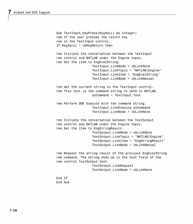
7 ActiveX and DDE Support
7-30
Sub TextInput_KeyPress(KeyAscii As Integer)rem If the user presses the return keyrem in the TextInput control.If KeyAscii = vbKeyReturn then
rem Initiate the conversation between the TextInputrem control and MATLAB under the Engine topic.rem Set the item to EngEvalString.
TextInput.LinkMode = vbLinkNoneTextInput.LinkTopic = "MATLAB|Engine"TextInput.LinkItem = "EngEvalString"TextInput.LinkMode = vbLinkManual
rem Get the current string in the TextInput control.rem This text is the command string to send to MATLAB.
szCommand = TextInput.Text
rem Perform DDE Execute with the command string.TextInput.LinkExecute szCommandTextInput.LinkMode = vbLinkNone
rem Initiate the conversation between the TextOutputrem control and MATLAB under the Engine topic.rem Set the item to EngStringResult.
TextOutput.LinkMode = vbLinkNoneTextOutput.LinkTopic = "MATLAB|Engine"TextOutput.LinkItem = "EngStringResult"TextOutput.LinkMode = vbLinkManual
rem Request the string result of the previous EngEvalStringrem command. The string ends up in the text field of therem control TextOutput.text.
TextOutput.LinkRequestTextOutput.LinkMode = vbLinkNone
End IfEnd Sub
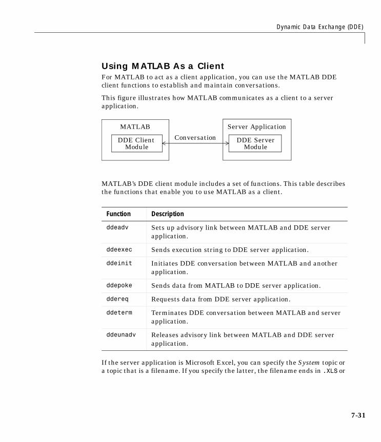
Dynamic Data Exchange (DDE)
7-31
Using MATLAB As a ClientFor MATLAB to act as a client application, you can use the MATLAB DDE client functions to establish and maintain conversations.
This figure illustrates how MATLAB communicates as a client to a server application.
MATLAB’s DDE client module includes a set of functions. This table describes the functions that enable you to use MATLAB as a client.
If the server application is Microsoft Excel, you can specify the System topic or a topic that is a filename. If you specify the latter, the filename ends in .XLS or
Function Description
ddeadv Sets up advisory link between MATLAB and DDE server application.
ddeexec Sends execution string to DDE server application.
ddeinit Initiates DDE conversation between MATLAB and another application.
ddepoke Sends data from MATLAB to DDE server application.
ddereq Requests data from DDE server application.
ddeterm Terminates DDE conversation between MATLAB and server application.
ddeunadv Releases advisory link between MATLAB and DDE server application.
MATLAB
DDE ClientModule
Server Application
Conversation DDE ServerModule
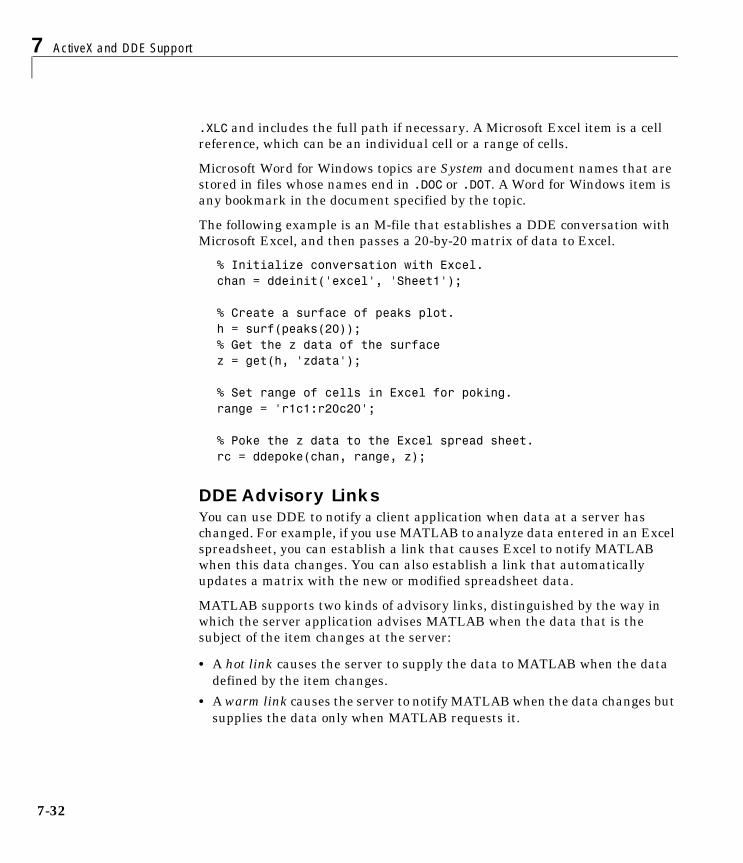
7 ActiveX and DDE Support
7-32
.XLC and includes the full path if necessary. A Microsoft Excel item is a cell reference, which can be an individual cell or a range of cells.
Microsoft Word for Windows topics are System and document names that are stored in files whose names end in .DOC or .DOT. A Word for Windows item is any bookmark in the document specified by the topic.
The following example is an M-file that establishes a DDE conversation with Microsoft Excel, and then passes a 20-by-20 matrix of data to Excel.
% Initialize conversation with Excel.chan = ddeinit('excel', 'Sheet1');
% Create a surface of peaks plot.h = surf(peaks(20));% Get the z data of the surfacez = get(h, 'zdata');
% Set range of cells in Excel for poking.range = 'r1c1:r20c20';
% Poke the z data to the Excel spread sheet.rc = ddepoke(chan, range, z);
DDE Advisory LinksYou can use DDE to notify a client application when data at a server has changed. For example, if you use MATLAB to analyze data entered in an Excel spreadsheet, you can establish a link that causes Excel to notify MATLAB when this data changes. You can also establish a link that automatically updates a matrix with the new or modified spreadsheet data.
MATLAB supports two kinds of advisory links, distinguished by the way in which the server application advises MATLAB when the data that is the subject of the item changes at the server:
• A hot link causes the server to supply the data to MATLAB when the data defined by the item changes.
• A warm link causes the server to notify MATLAB when the data changes but supplies the data only when MATLAB requests it.
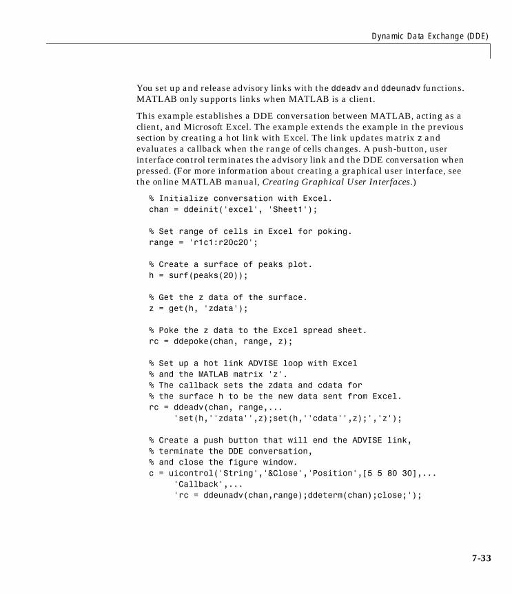
Dynamic Data Exchange (DDE)
7-33
You set up and release advisory links with the ddeadv and ddeunadv functions. MATLAB only supports links when MATLAB is a client.
This example establishes a DDE conversation between MATLAB, acting as a client, and Microsoft Excel. The example extends the example in the previous section by creating a hot link with Excel. The link updates matrix z and evaluates a callback when the range of cells changes. A push-button, user interface control terminates the advisory link and the DDE conversation when pressed. (For more information about creating a graphical user interface, see the online MATLAB manual, Creating Graphical User Interfaces.)
% Initialize conversation with Excel.chan = ddeinit('excel', 'Sheet1');
% Set range of cells in Excel for poking.range = 'r1c1:r20c20';
% Create a surface of peaks plot.h = surf(peaks(20));
% Get the z data of the surface.z = get(h, 'zdata');
% Poke the z data to the Excel spread sheet.rc = ddepoke(chan, range, z);
% Set up a hot link ADVISE loop with Excel% and the MATLAB matrix 'z'.% The callback sets the zdata and cdata for% the surface h to be the new data sent from Excel.rc = ddeadv(chan, range,...
'set(h,''zdata'',z);set(h,''cdata'',z);','z');
% Create a push button that will end the ADVISE link,% terminate the DDE conversation,% and close the figure window.c = uicontrol('String','&Close','Position',[5 5 80 30],...
'Callback',...'rc = ddeunadv(chan,range);ddeterm(chan);close;');

7 ActiveX and DDE Support
7-34

8
Serial Port I/O
Introduction . . . . . . . . . . . . . . . . . . . . 8-2
Overview of the Serial Port . . . . . . . . . . . . . 8-4
Getting Started with Serial I/O . . . . . . . . . . . 8-18
Creating a Serial Port Object . . . . . . . . . . . . 8-24
Connecting to the Device . . . . . . . . . . . . . . 8-27
Configuring Communication Settings . . . . . . . . 8-28
Writing and Reading Data . . . . . . . . . . . . . . 8-29
Events and Callbacks . . . . . . . . . . . . . . . . 8-48
Using Control Pins . . . . . . . . . . . . . . . . . 8-56
Debugging: Recording Information to Disk . . . . . . 8-62
Saving and Loading . . . . . . . . . . . . . . . . 8-68
Disconnecting and Cleaning Up . . . . . . . . . . . 8-69
Property Reference . . . . . . . . . . . . . . . . . 8-70
8 Serial Port I/O
8-2
Introduction
What Is MATLAB’s Serial Port Interface?MATLAB’s serial port interface provides direct access to peripheral devices such as modems, printers, and scientific instruments that you connect to your computer’s serial port. This interface is established through a serial port object. The serial port object supports functions and properties that allow you to:
• Configure serial port communications
• Use serial port control pins
• Write and read data
• Use events and callbacks
• Record information to disk
If you want to communicate with PC-compatible data acquisition hardware such as multifunction I/O boards, you need the Data Acquisition Toolbox. If you want to communicate with GPIB- or VISA-compatible instruments, you need the Instrument Control Toolbox.
For more information about these products, visit the MathWorks Web site at http://www.mathworks.com/products.
Supported Serial Port Interface StandardsOver the years, several serial port interface standards have been developed. These standards include RS-232, RS-422, and RS-485 – all of which are supported by MATLAB’s serial port object. Of these, the most widely used interface standard for connecting computers to peripheral devices is RS-232.
In this guide, it is assumed you are using the RS-232 standard, which is discussed in “Overview of the Serial Port” on page 8-4. Refer to your computer and device documentation to see which interface standard you can use.
Supported PlatformsMATLAB’s serial port interface is supported for Microsoft Windows 95, Windows 98, Windows 2000, Windows NT, Linux, and Sun Solaris platforms.
8-3
Using the Examples with Your DeviceMany of the examples in this section reflect specific peripheral devices connected to a PC serial port – in particular a Tektronix TDS 210 two-channel oscilloscope connected to the COM1 port. Therefore, many of the string commands are specific to this instrument.
If your peripheral device is connected to a different serial port, or if it accepts different commands, you should modify the examples accordingly.
8 Serial Port I/O
8-4
Overview of the Serial PortThis section provides an overview of the serial port. Topics include:
• What is Serial Communication?
• The Serial Port Interface Standard
• Connecting Two Devices with a Serial Cable
• Serial Port Signals and Pin Assignments
• Serial Data Format
• Finding Serial Port Information for Your Platform
For many serial port applications, you can communicate with your device without detailed knowledge of how the serial port works. If your application is straightforward, or if you are already familiar with the topics mentioned above, you may want to begin with “The Serial Port Session” on page 8-19 to see how to use your serial port device with MATLAB.
What Is Serial Communication?Serial communication is the most common low-level protocol for communicating between two or more devices. Normally, one device is a computer, while the other device can be a modem, a printer, another computer, or a scientific instrument such as an oscilloscope or a function generator.
As the name suggests, the serial port sends and receives bytes of information in a serial fashion – one bit at a time. These bytes are transmitted using either a binary (numerical) format or a text format.
The Serial Port Interface StandardThe serial port interface for connecting two devices is specified by the TIA/EIA-232C standard published by the Telecommunications Industry Association.
The original serial port interface standard was given by RS-232, which stands for Recommended Standard number 232. The term “RS-232” is still in popular use, and is used in this guide when referring to a serial communication port that follows the TIA/EIA-232 standard. RS-232 defines these serial port characteristics:
• The maximum bit transfer rate and cable length
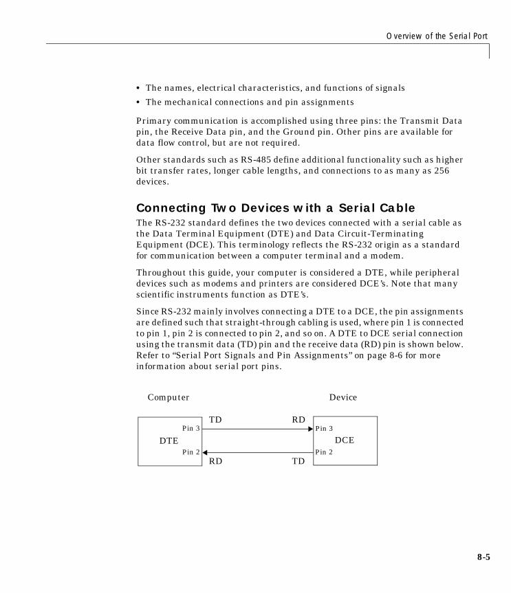
Overview of the Serial Port
8-5
• The names, electrical characteristics, and functions of signals
• The mechanical connections and pin assignments
Primary communication is accomplished using three pins: the Transmit Data pin, the Receive Data pin, and the Ground pin. Other pins are available for data flow control, but are not required.
Other standards such as RS-485 define additional functionality such as higher bit transfer rates, longer cable lengths, and connections to as many as 256 devices.
Connecting Two Devices with a Serial CableThe RS-232 standard defines the two devices connected with a serial cable as the Data Terminal Equipment (DTE) and Data Circuit-Terminating Equipment (DCE). This terminology reflects the RS-232 origin as a standard for communication between a computer terminal and a modem.
Throughout this guide, your computer is considered a DTE, while peripheral devices such as modems and printers are considered DCE’s. Note that many scientific instruments function as DTE’s.
Since RS-232 mainly involves connecting a DTE to a DCE, the pin assignments are defined such that straight-through cabling is used, where pin 1 is connected to pin 1, pin 2 is connected to pin 2, and so on. A DTE to DCE serial connection using the transmit data (TD) pin and the receive data (RD) pin is shown below. Refer to “Serial Port Signals and Pin Assignments” on page 8-6 for more information about serial port pins.
DTE DCEPin 2
Pin 3
Pin 2
Pin 3
RD TD
TD RD
Computer Device
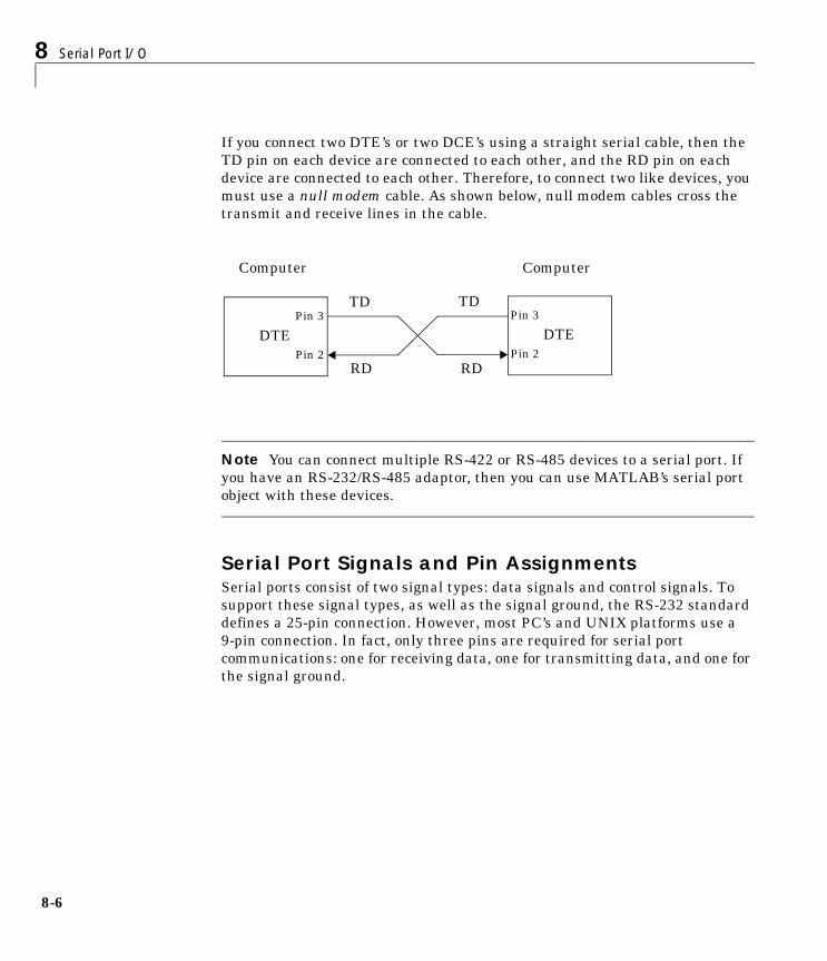
8 Serial Port I/O
8-6
If you connect two DTE’s or two DCE’s using a straight serial cable, then the TD pin on each device are connected to each other, and the RD pin on each device are connected to each other. Therefore, to connect two like devices, you must use a null modem cable. As shown below, null modem cables cross the transmit and receive lines in the cable.
Note You can connect multiple RS-422 or RS-485 devices to a serial port. If you have an RS-232/RS-485 adaptor, then you can use MATLAB’s serial port object with these devices.
Serial Port Signals and Pin AssignmentsSerial ports consist of two signal types: data signals and control signals. To support these signal types, as well as the signal ground, the RS-232 standard defines a 25-pin connection. However, most PC’s and UNIX platforms use a 9-pin connection. In fact, only three pins are required for serial port communications: one for receiving data, one for transmitting data, and one for the signal ground.
DTE DTE
TD
Pin 2
Pin 3
Pin 2
Pin 3TD
RDRD
Computer Computer
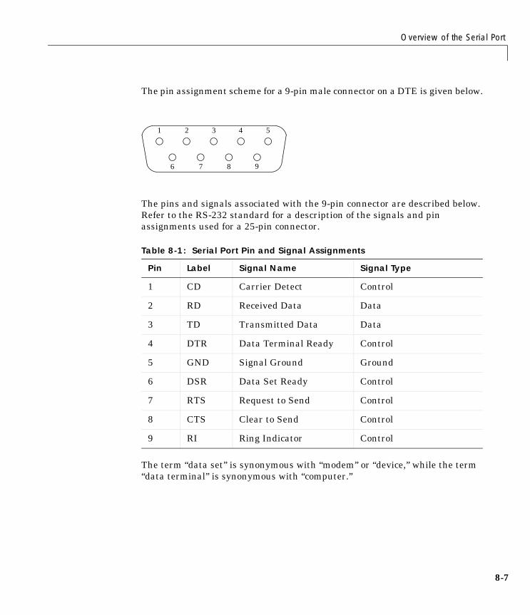
Overview of the Serial Port
8-7
The pin assignment scheme for a 9-pin male connector on a DTE is given below.
The pins and signals associated with the 9-pin connector are described below. Refer to the RS-232 standard for a description of the signals and pin assignments used for a 25-pin connector.
The term “data set” is synonymous with “modem” or “device,” while the term “data terminal” is synonymous with “computer.”
Table 8-1: Serial Port Pin and Signal Assignments
Pin Label Signal Name Signal Type
1 CD Carrier Detect Control
2 RD Received Data Data
3 TD Transmitted Data Data
4 DTR Data Terminal Ready Control
5 GND Signal Ground Ground
6 DSR Data Set Ready Control
7 RTS Request to Send Control
8 CTS Clear to Send Control
9 RI Ring Indicator Control
1 2 3 4 5
6 7 8 9
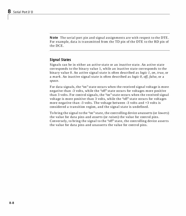
8 Serial Port I/O
8-8
Note The serial port pin and signal assignments are with respect to the DTE. For example, data is transmitted from the TD pin of the DTE to the RD pin of the DCE.
Signal StatesSignals can be in either an active state or an inactive state. An active state corresponds to the binary value 1, while an inactive state corresponds to the binary value 0. An active signal state is often described as logic 1, on, true, or a mark. An inactive signal state is often described as logic 0, off, false, or a space.
For data signals, the “on” state occurs when the received signal voltage is more negative than -3 volts, while the “off” state occurs for voltages more positive than 3 volts. For control signals, the “on” state occurs when the received signal voltage is more positive than 3 volts, while the “off” state occurs for voltages more negative than -3 volts. The voltage between -3 volts and +3 volts is considered a transition region, and the signal state is undefined.
To bring the signal to the “on” state, the controlling device unasserts (or lowers) the value for data pins and asserts (or raises) the value for control pins. Conversely, to bring the signal to the “off” state, the controlling device asserts the value for data pins and unasserts the value for control pins.
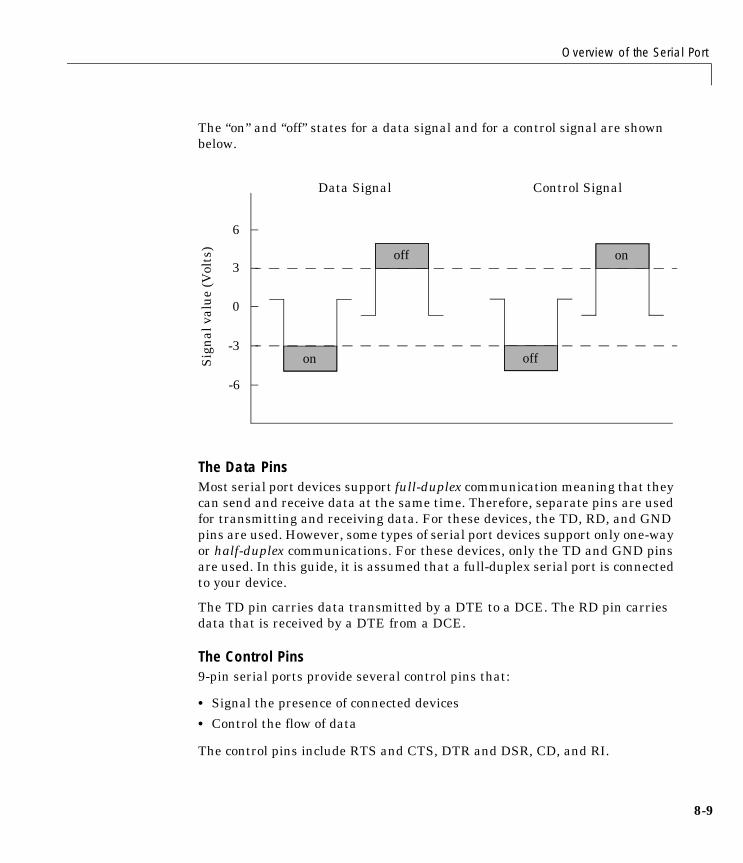
Overview of the Serial Port
8-9
The “on” and “off” states for a data signal and for a control signal are shown below.
The Data PinsMost serial port devices support full-duplex communication meaning that they can send and receive data at the same time. Therefore, separate pins are used for transmitting and receiving data. For these devices, the TD, RD, and GND pins are used. However, some types of serial port devices support only one-way or half-duplex communications. For these devices, only the TD and GND pins are used. In this guide, it is assumed that a full-duplex serial port is connected to your device.
The TD pin carries data transmitted by a DTE to a DCE. The RD pin carries data that is received by a DTE from a DCE.
The Control Pins9-pin serial ports provide several control pins that:
• Signal the presence of connected devices
• Control the flow of data
The control pins include RTS and CTS, DTR and DSR, CD, and RI.
-6
Sig
nal
val
ue
(Vol
ts)
-3
0
3
6
Data Signal Control Signal
on
off
off
on
8 Serial Port I/O
8-10
The RTS and CTS Pins. The RTS and CTS pins are used to signal whether the devices are ready to send or receive data. This type of data flow control – called hardware handshaking – is used to prevent data loss during transmission. When enabled for both the DTE and DCE, hardware handshaking using RTS and CTS follows these steps:
1 The DTE asserts the RTS pin to instruct the DCE that it is ready to receive data.
2 The DCE asserts the CTS pin indicating that it is clear to send data over the TD pin. If data can no longer be sent, the CTS pin is unasserted.
3 The data is transmitted to the DTE over the TD pin. If data can no longer be accepted, the RTS pin is unasserted by the DTE and the data transmission is stopped.
To enable hardware handshaking in MATLAB, refer to “Controlling the Flow of Data: Handshaking” on page 8-59.
The DTR and DSR Pins. Many devices use the DSR and DTR pins to signal if they are connected and powered. Signaling the presence of connected devices using DTR and DSR follows these steps:
1 The DTE asserts the DTR pin to request that the DCE connect to the communication line.
2 The DCE asserts the DSR pin to indicate it’s connected.
3 DCE unasserts the DSR pin when it’s disconnected from the communication line.
The DTR and DSR pins were originally designed to provide an alternative method of hardware handshaking. However, the RTS and CTS pins are usually used in this way, and not the DSR and DTR pins. However, you should refer to your device documentation to determine its specific pin behavior.
The CD and RI Pins. The CD and RI pins are typically used to indicate the presence of certain signals during modem-modem connections.
CD is used by a modem to signal that it has made a connection with another modem, or has detected a carrier tone. CD is asserted when the DCE is
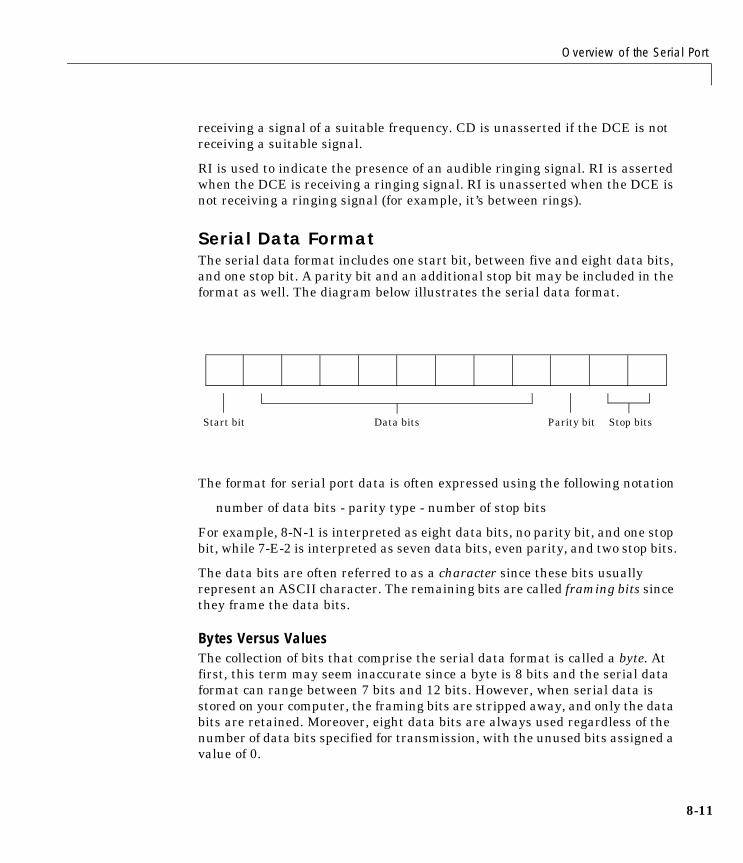
Overview of the Serial Port
8-11
receiving a signal of a suitable frequency. CD is unasserted if the DCE is not receiving a suitable signal.
RI is used to indicate the presence of an audible ringing signal. RI is asserted when the DCE is receiving a ringing signal. RI is unasserted when the DCE is not receiving a ringing signal (for example, it’s between rings).
Serial Data FormatThe serial data format includes one start bit, between five and eight data bits, and one stop bit. A parity bit and an additional stop bit may be included in the format as well. The diagram below illustrates the serial data format.
The format for serial port data is often expressed using the following notation
number of data bits - parity type - number of stop bits
For example, 8-N-1 is interpreted as eight data bits, no parity bit, and one stop bit, while 7-E-2 is interpreted as seven data bits, even parity, and two stop bits.
The data bits are often referred to as a character since these bits usually represent an ASCII character. The remaining bits are called framing bits since they frame the data bits.
Bytes Versus ValuesThe collection of bits that comprise the serial data format is called a byte. At first, this term may seem inaccurate since a byte is 8 bits and the serial data format can range between 7 bits and 12 bits. However, when serial data is stored on your computer, the framing bits are stripped away, and only the data bits are retained. Moreover, eight data bits are always used regardless of the number of data bits specified for transmission, with the unused bits assigned a value of 0.
Start bit Data bits Parity bit Stop bits
8 Serial Port I/O
8-12
When reading or writing data, you may need to specify a value, which can consist of one or more bytes. For example, if you read one value from a device using the int32 format, then that value consists of four bytes. For more information about reading and writing values, refer to “Writing and Reading Data” on page 8-29.
Synchronous and Asynchronous CommunicationThe RS-232 standard supports two types of communication protocols: synchronous and asynchronous.
Using the synchronous protocol, all transmitted bits are synchronized to a common clock signal. The two devices initially synchronize themselves to each other, and then continually send characters to stay synchronized. Even when actual data is not really being sent, a constant flow of bits allows each device to know where the other is at any given time. That is, each bit that is sent is either actual data or an idle character. Synchronous communications allows faster data transfer rates than asynchronous methods, because additional bits to mark the beginning and end of each data byte are not required.
Using the asynchronous protocol, each device uses its own internal clock resulting in bytes that are transferred at arbitrary times. So, instead of using time as a way to synchronize the bits, the data format is used.
In particular, the data transmission is synchronized using the start bit of the word, while one or more stop bits indicate the end of the word. The requirement to send these additional bits causes asynchronous communications to be slightly slower than synchronous. However, it has the advantage that the processor does not have to deal with the additional idle characters. Most serial ports operate asynchronously.
Note When used in this guide, the terms “synchronous” and “asynchronous” refer to whether read or write operations block access to the MATLAB command line. Refer to “Controlling Access to the MATLAB Command Line” on page 8-29 for more information.
How Are the Bits Transmitted?By definition, serial data is transmitted one bit at a time. The order in which the bits are transmitted is given below:

Overview of the Serial Port
8-13
1 The start bit is transmitted with a value of 0.
2 The data bits are transmitted. The first data bit corresponds to the least significant bit (LSB), while the last data bit corresponds to the most significant bit (MSB).
3 The parity bit (if defined) is transmitted.
4 One or two stop bits are transmitted, each with a value of 1.
The number of bits transferred per second is given by the baud rate. The transferred bits include the start bit, the data bits, the parity bit (if defined), and the stop bits.
Start and Stop BitsAs described in “Synchronous and Asynchronous Communication” on page 8-12, most serial ports operate asynchronously. This means that the transmitted byte must be identified by start and stop bits. The start bit indicates when the data byte is about to begin and the stop bit(s) indicates when the data byte has been transferred. The process of identifying bytes with the serial data format follows these steps:
1 When a serial port pin is idle (not transmitting data), then it is in an “on” state.
2 When data is about to be transmitted, the serial port pin switches to an “off” state due to the start bit.
3 The serial port pin switches back to an “on” state due to the stop bit(s). This indicates the end of the byte.
Data BitsThe data bits transferred through a serial port may represent device commands, sensor readings, error messages, and so on. The data can be transferred as either binary data or ASCII data.
Most serial ports use between five and eight data bits. Binary data is typically transmitted as eight bits. Text-based data is transmitted as either seven bits or eight bits. If the data is based on the ASCII character set, then a minimum of seven bits is required since there are 27 or 128 distinct characters. If an
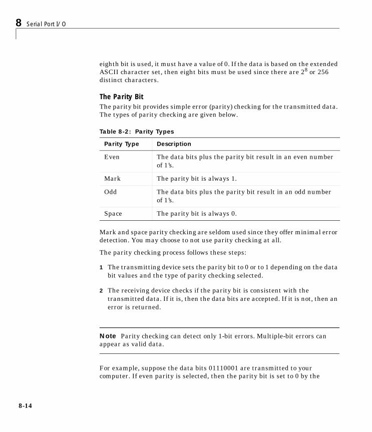
8 Serial Port I/O
8-14
eighth bit is used, it must have a value of 0. If the data is based on the extended ASCII character set, then eight bits must be used since there are 28 or 256 distinct characters.
The Parity BitThe parity bit provides simple error (parity) checking for the transmitted data. The types of parity checking are given below.
Mark and space parity checking are seldom used since they offer minimal error detection. You may choose to not use parity checking at all.
The parity checking process follows these steps:
1 The transmitting device sets the parity bit to 0 or to 1 depending on the data bit values and the type of parity checking selected.
2 The receiving device checks if the parity bit is consistent with the transmitted data. If it is, then the data bits are accepted. If it is not, then an error is returned.
Note Parity checking can detect only 1-bit errors. Multiple-bit errors can appear as valid data.
For example, suppose the data bits 01110001 are transmitted to your computer. If even parity is selected, then the parity bit is set to 0 by the
Table 8-2: Parity Types
Parity Type Description
Even The data bits plus the parity bit result in an even number of 1’s.
Mark The parity bit is always 1.
Odd The data bits plus the parity bit result in an odd number of 1’s.
Space The parity bit is always 0.
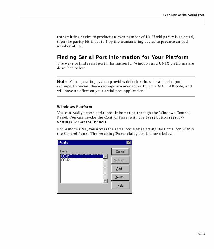
Overview of the Serial Port
8-15
transmitting device to produce an even number of 1’s. If odd parity is selected, then the parity bit is set to 1 by the transmitting device to produce an odd number of 1’s.
Finding Serial Port Information for Your PlatformThe ways to find serial port information for Windows and UNIX platforms are described below.
Note Your operating system provides default values for all serial port settings. However, these settings are overridden by your MATLAB code, and will have no effect on your serial port application.
Windows PlatformYou can easily access serial port information through the Windows Control Panel. You can invoke the Control Panel with the Start button (Start -> Settings -> Control Panel).
For Windows NT, you access the serial ports by selecting the Ports icon within the Control Panel. The resulting Ports dialog box is shown below.
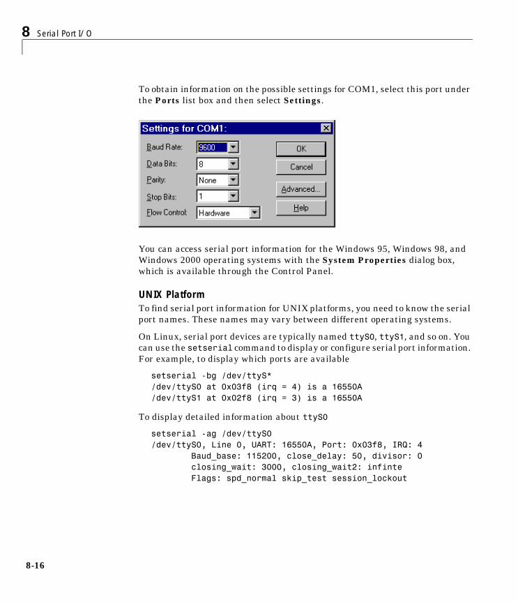
8 Serial Port I/O
8-16
To obtain information on the possible settings for COM1, select this port under the Ports list box and then select Settings.
You can access serial port information for the Windows 95, Windows 98, and Windows 2000 operating systems with the System Properties dialog box, which is available through the Control Panel.
UNIX PlatformTo find serial port information for UNIX platforms, you need to know the serial port names. These names may vary between different operating systems.
On Linux, serial port devices are typically named ttyS0, ttyS1, and so on. You can use the setserial command to display or configure serial port information. For example, to display which ports are available
setserial -bg /dev/ttyS*/dev/ttyS0 at 0x03f8 (irq = 4) is a 16550A/dev/ttyS1 at 0x02f8 (irq = 3) is a 16550A
To display detailed information about ttyS0
setserial -ag /dev/ttyS0/dev/ttyS0, Line 0, UART: 16550A, Port: 0x03f8, IRQ: 4 Baud_base: 115200, close_delay: 50, divisor: 0 closing_wait: 3000, closing_wait2: infinte Flags: spd_normal skip_test session_lockout
Overview of the Serial Port
8-17
Note If the setserial -ag command does not work, make sure that you have read and write permission for the port.
For all supported UNIX platforms, you can use the stty command to display or configure serial port information. For example, to display serial port properties for ttyS0
stty -a < /dev/ttyS0
To configure the baud rate to 4800 bits per second
stty speed 4800 < /dev/ttyS0 > /dev/ttyS0
Selected Bibliography
1 TIA/EIA-232-F, Interface Between Data Terminal Equipment and Data Circuit-Terminating Equipment Employing Serial Binary Data Interchange.
2 Jan Axelson, Serial Port Complete, Lakeview Research, Madison, WI, 1998.
3 Instrument Communication Handbook, IOTech, Inc., Cleveland, OH, 1991.
4 TDS 200-Series Two Channel Digital Oscilloscope Programmer Manual, Tektronix, Inc., Wilsonville, OR.
5 Courier High Speed Modems User’s Manual, U.S. Robotics, Inc., Skokie, IL, 1994.
6 Getting Started with Your AT Serial Hardware and Software for Windows 98/95, National Instruments, Inc., Austin, TX, 1998.
8 Serial Port I/O
8-18
Getting Started with Serial I/OTo get you started with MATLAB’s serial port interface, this section provides the following information:
• “Example: Getting Started” illustrates some basic serial port commands.
• “The Serial Port Session” describes the steps you use to perform any serial port task from beginning to end.
• “Configuring and Returning Properties” describes how you display serial port property names and property values, and how you assign values to properties.
Example: Getting StartedIf you have a device connected to the serial port COM1 and configured for a baud rate of 4800, you can execute the following complete example.
s = serial('COM1');set(s,'BaudRate',4800);fopen(s);fprintf(s,'*IDN?')out = fscanf(s);fclose(s)delete(s)clear s
The *IDN? command queries the device for identification information, which is returned to out. If your device does not support this command, or if it is connected to a different serial port, you should modify the above example accordingly.
Note *IDN? is one of the commands supported by the Standard Commands for Programmable Instruments (SCPI) language, which is used by many modern devices. Refer to your device documentation to see if it supports the SCPI language.
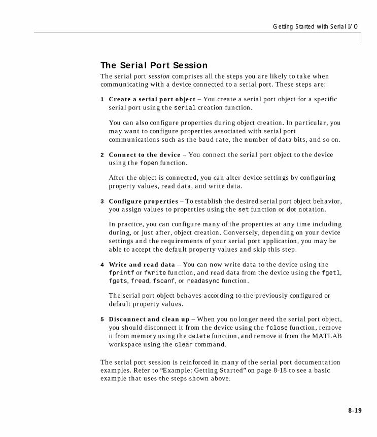
Getting Started with Serial I/O
8-19
The Serial Port SessionThe serial port session comprises all the steps you are likely to take when communicating with a device connected to a serial port. These steps are:
1 Create a serial port object – You create a serial port object for a specific serial port using the serial creation function.
You can also configure properties during object creation. In particular, you may want to configure properties associated with serial port communications such as the baud rate, the number of data bits, and so on.
2 Connect to the device – You connect the serial port object to the device using the fopen function.
After the object is connected, you can alter device settings by configuring property values, read data, and write data.
3 Configure properties – To establish the desired serial port object behavior, you assign values to properties using the set function or dot notation.
In practice, you can configure many of the properties at any time including during, or just after, object creation. Conversely, depending on your device settings and the requirements of your serial port application, you may be able to accept the default property values and skip this step.
4 Write and read data – You can now write data to the device using the fprintf or fwrite function, and read data from the device using the fgetl, fgets, fread, fscanf, or readasync function.
The serial port object behaves according to the previously configured or default property values.
5 Disconnect and clean up – When you no longer need the serial port object, you should disconnect it from the device using the fclose function, remove it from memory using the delete function, and remove it from the MATLAB workspace using the clear command.
The serial port session is reinforced in many of the serial port documentation examples. Refer to “Example: Getting Started” on page 8-18 to see a basic example that uses the steps shown above.
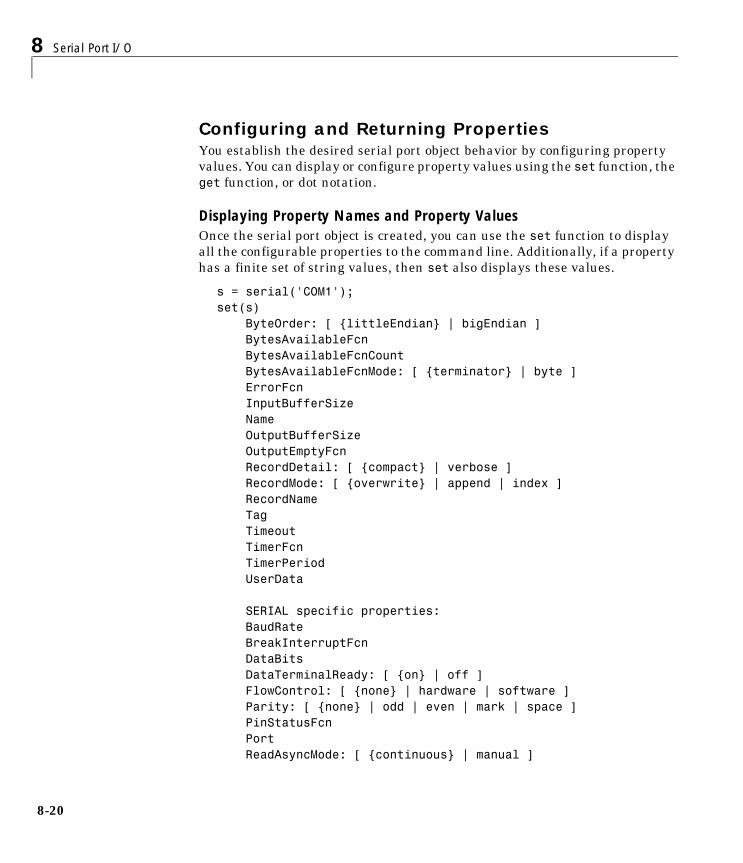
8 Serial Port I/O
8-20
Configuring and Returning PropertiesYou establish the desired serial port object behavior by configuring property values. You can display or configure property values using the set function, the get function, or dot notation.
Displaying Property Names and Property ValuesOnce the serial port object is created, you can use the set function to display all the configurable properties to the command line. Additionally, if a property has a finite set of string values, then set also displays these values.
s = serial('COM1');set(s)
ByteOrder: [ {littleEndian} | bigEndian ] BytesAvailableFcn BytesAvailableFcnCount BytesAvailableFcnMode: [ {terminator} | byte ] ErrorFcn InputBufferSize Name OutputBufferSize OutputEmptyFcn RecordDetail: [ {compact} | verbose ] RecordMode: [ {overwrite} | append | index ] RecordName Tag Timeout TimerFcn TimerPeriod UserData
SERIAL specific properties: BaudRate BreakInterruptFcn DataBits DataTerminalReady: [ {on} | off ] FlowControl: [ {none} | hardware | software ] Parity: [ {none} | odd | even | mark | space ] PinStatusFcn Port ReadAsyncMode: [ {continuous} | manual ]
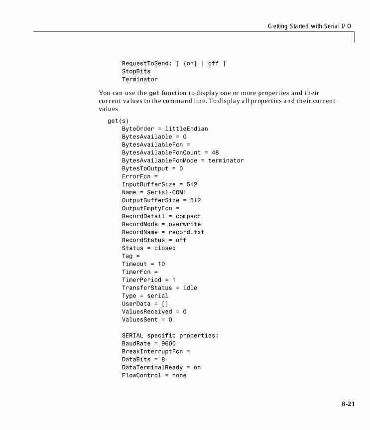
Getting Started with Serial I/O
8-21
RequestToSend: [ {on} | off ] StopBits Terminator
You can use the get function to display one or more properties and their current values to the command line. To display all properties and their current values
get(s)ByteOrder = littleEndian
BytesAvailable = 0 BytesAvailableFcn = BytesAvailableFcnCount = 48 BytesAvailableFcnMode = terminator BytesToOutput = 0 ErrorFcn = InputBufferSize = 512 Name = Serial-COM1 OutputBufferSize = 512 OutputEmptyFcn = RecordDetail = compact RecordMode = overwrite RecordName = record.txt RecordStatus = off Status = closed Tag = Timeout = 10 TimerFcn = TimerPeriod = 1 TransferStatus = idle Type = serial UserData = [] ValuesReceived = 0 ValuesSent = 0
SERIAL specific properties: BaudRate = 9600 BreakInterruptFcn = DataBits = 8 DataTerminalReady = on FlowControl = none

8 Serial Port I/O
8-22
Parity = none PinStatus = [1x1 struct] PinStatusFcn = Port = COM1 ReadAsyncMode = continuous RequestToSend = on StopBits = 1 Terminator = LF
To display the current value for one property, you supply the property name to get.
get(s,'OutputBufferSize')ans = 512
To display the current values for multiple properties, you must include the property names as elements of a cell array.
get(s,{'Parity','TransferStatus'})ans = 'none' 'idle'
You can also use the dot notation to display a single property value.
s.Parityans =none
Configuring Property ValuesYou can configure property values using the set function
set(s,'BaudRate',4800);
or the dot notation.
s.BaudRate = 4800;
To configure values for multiple properties, you can supply multiple property name/property value pairs to set.
set(s,'DataBits',7,'Name','Test1-serial')
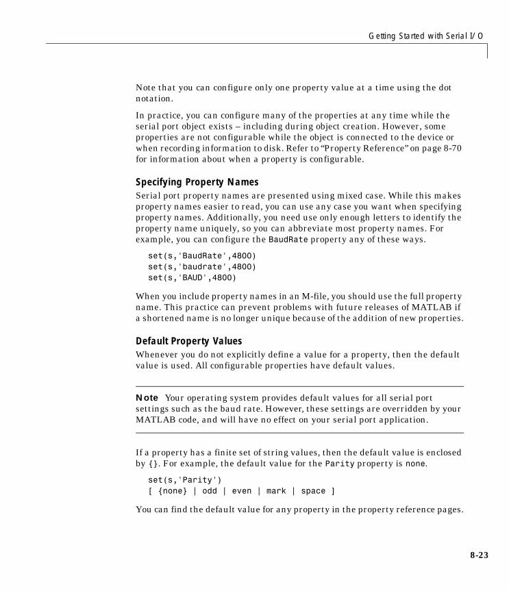
Getting Started with Serial I/O
8-23
Note that you can configure only one property value at a time using the dot notation.
In practice, you can configure many of the properties at any time while the serial port object exists – including during object creation. However, some properties are not configurable while the object is connected to the device or when recording information to disk. Refer to “Property Reference” on page 8-70 for information about when a property is configurable.
Specifying Property NamesSerial port property names are presented using mixed case. While this makes property names easier to read, you can use any case you want when specifying property names. Additionally, you need use only enough letters to identify the property name uniquely, so you can abbreviate most property names. For example, you can configure the BaudRate property any of these ways.
set(s,'BaudRate',4800)set(s,'baudrate',4800)set(s,'BAUD',4800)
When you include property names in an M-file, you should use the full property name. This practice can prevent problems with future releases of MATLAB if a shortened name is no longer unique because of the addition of new properties.
Default Property ValuesWhenever you do not explicitly define a value for a property, then the default value is used. All configurable properties have default values.
Note Your operating system provides default values for all serial port settings such as the baud rate. However, these settings are overridden by your MATLAB code, and will have no effect on your serial port application.
If a property has a finite set of string values, then the default value is enclosed by {}. For example, the default value for the Parity property is none.
set(s,'Parity')[ {none} | odd | even | mark | space ]
You can find the default value for any property in the property reference pages.
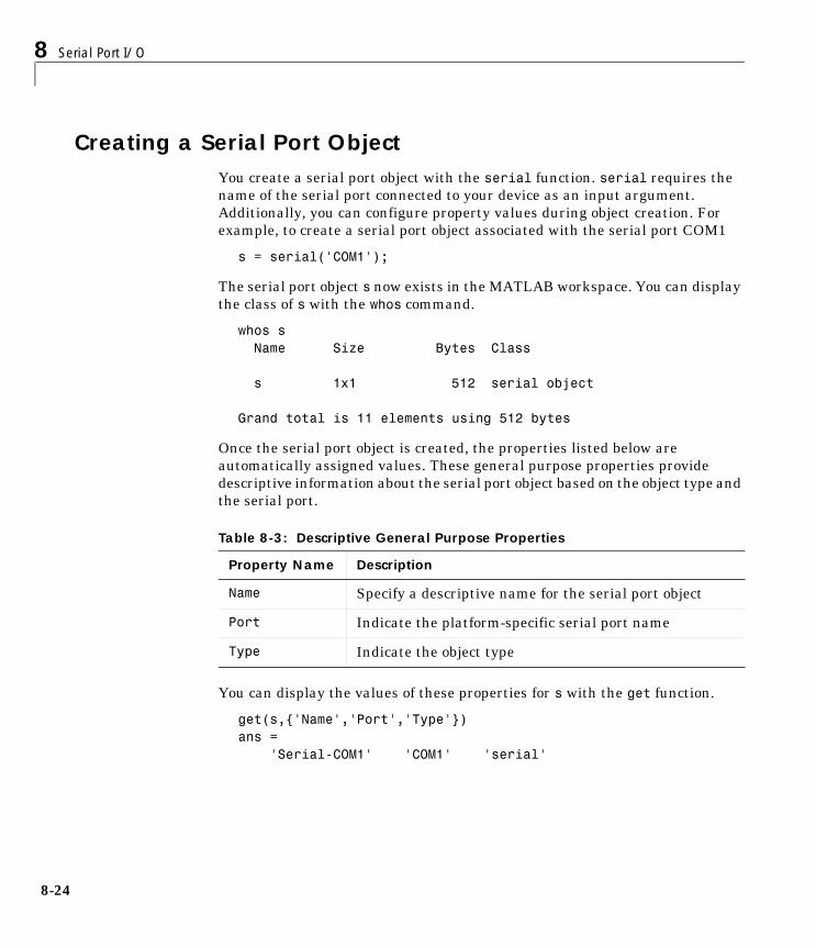
8 Serial Port I/O
8-24
Creating a Serial Port ObjectYou create a serial port object with the serial function. serial requires the name of the serial port connected to your device as an input argument. Additionally, you can configure property values during object creation. For example, to create a serial port object associated with the serial port COM1
s = serial('COM1');
The serial port object s now exists in the MATLAB workspace. You can display the class of s with the whos command.
whos s Name Size Bytes Class
s 1x1 512 serial object
Grand total is 11 elements using 512 bytes
Once the serial port object is created, the properties listed below are automatically assigned values. These general purpose properties provide descriptive information about the serial port object based on the object type and the serial port.
You can display the values of these properties for s with the get function.
get(s,{'Name','Port','Type'})ans = 'Serial-COM1' 'COM1' 'serial'
Table 8-3: Descriptive General Purpose Properties
Property Name Description
Name Specify a descriptive name for the serial port object
Port Indicate the platform-specific serial port name
Type Indicate the object type
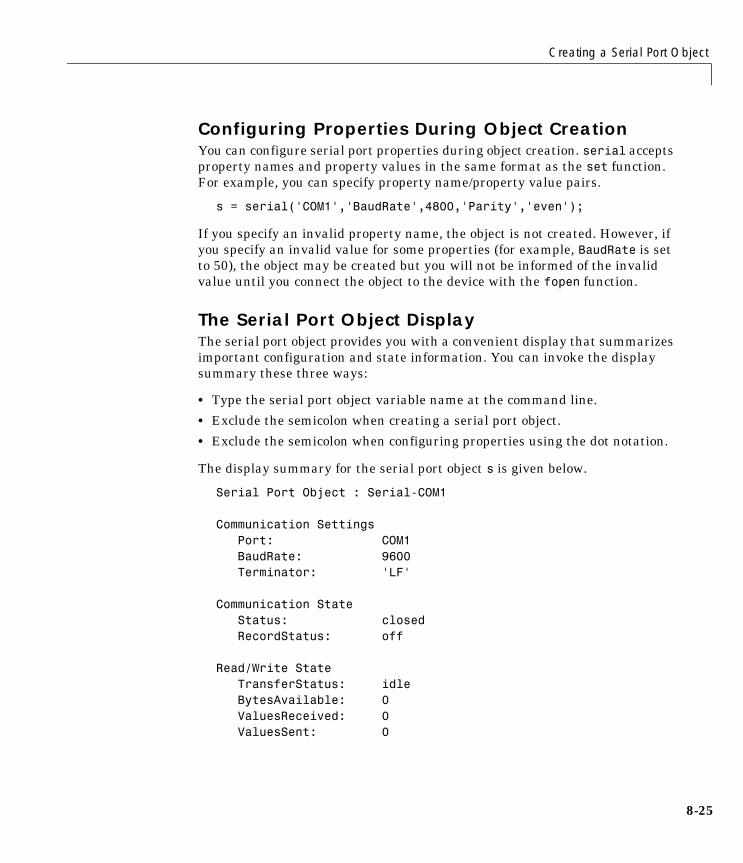
Creating a Serial Port Object
8-25
Configuring Properties During Object CreationYou can configure serial port properties during object creation. serial accepts property names and property values in the same format as the set function. For example, you can specify property name/property value pairs.
s = serial('COM1','BaudRate',4800,'Parity','even');
If you specify an invalid property name, the object is not created. However, if you specify an invalid value for some properties (for example, BaudRate is set to 50), the object may be created but you will not be informed of the invalid value until you connect the object to the device with the fopen function.
The Serial Port Object DisplayThe serial port object provides you with a convenient display that summarizes important configuration and state information. You can invoke the display summary these three ways:
• Type the serial port object variable name at the command line.
• Exclude the semicolon when creating a serial port object.
• Exclude the semicolon when configuring properties using the dot notation.
The display summary for the serial port object s is given below.
Serial Port Object : Serial-COM1
Communication Settings Port: COM1BaudRate: 9600Terminator: 'LF'
Communication State Status: closedRecordStatus: off
Read/Write State TransferStatus: idleBytesAvailable: 0ValuesReceived: 0ValuesSent: 0
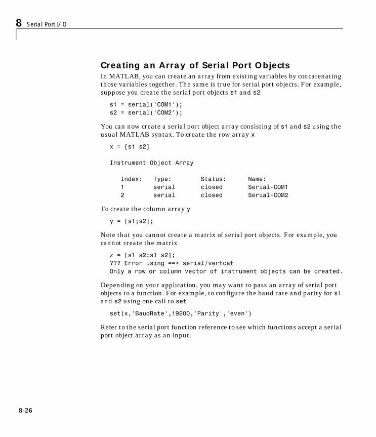
8 Serial Port I/O
8-26
Creating an Array of Serial Port ObjectsIn MATLAB, you can create an array from existing variables by concatenating those variables together. The same is true for serial port objects. For example, suppose you create the serial port objects s1 and s2
s1 = serial('COM1');s2 = serial('COM2');
You can now create a serial port object array consisting of s1 and s2 using the usual MATLAB syntax. To create the row array x
x = [s1 s2]
Instrument Object Array
Index: Type: Status: Name: 1 serial closed Serial-COM1 2 serial closed Serial-COM2
To create the column array y
y = [s1;s2];
Note that you cannot create a matrix of serial port objects. For example, you cannot create the matrix
z = [s1 s2;s1 s2];??? Error using ==> serial/vertcatOnly a row or column vector of instrument objects can be created.
Depending on your application, you may want to pass an array of serial port objects to a function. For example, to configure the baud rate and parity for s1 and s2 using one call to set
set(x,'BaudRate',19200,'Parity','even')
Refer to the serial port function reference to see which functions accept a serial port object array as an input.
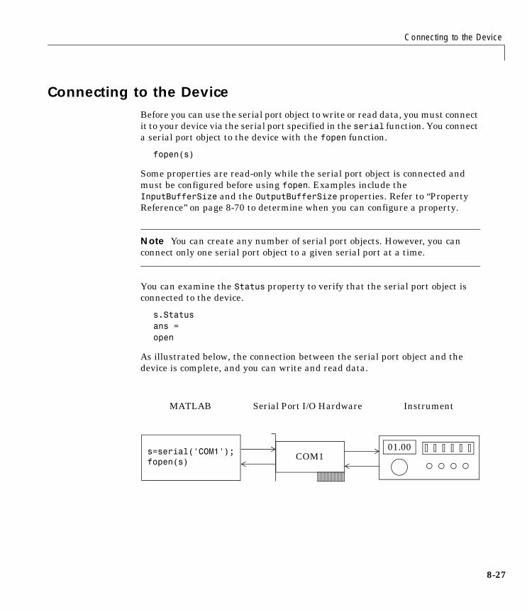
Connecting to the Device
8-27
Connecting to the DeviceBefore you can use the serial port object to write or read data, you must connect it to your device via the serial port specified in the serial function. You connect a serial port object to the device with the fopen function.
fopen(s)
Some properties are read-only while the serial port object is connected and must be configured before using fopen. Examples include the InputBufferSize and the OutputBufferSize properties. Refer to “Property Reference” on page 8-70 to determine when you can configure a property.
Note You can create any number of serial port objects. However, you can connect only one serial port object to a given serial port at a time.
You can examine the Status property to verify that the serial port object is connected to the device.
s.Statusans =open
As illustrated below, the connection between the serial port object and the device is complete, and you can write and read data.
Serial Port I/O Hardware
s=serial('COM1');fopen(s)
01.00COM1
InstrumentMATLAB
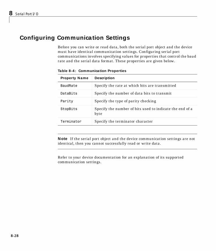
8 Serial Port I/O
8-28
Configuring Communication SettingsBefore you can write or read data, both the serial port object and the device must have identical communication settings. Configuring serial port communications involves specifying values for properties that control the baud rate and the serial data format. These properties are given below.
Note If the serial port object and the device communication settings are not identical, then you cannot successfully read or write data.
Refer to your device documentation for an explanation of its supported communication settings.
Table 8-4: Communication Properties
Property Name Description
BaudRate Specify the rate at which bits are transmitted
DataBits Specify the number of data bits to transmit
Parity Specify the type of parity checking
StopBits Specify the number of bits used to indicate the end of a byte
Terminator Specify the terminator character
Writing and Reading Data
8-29
Writing and Reading DataFor many serial port applications, there are three important questions that you should consider when writing or reading data:
• Will the read or write function block access to the MATLAB command line?
• Is the data to be transferred binary (numerical) or text?
• Under what conditions will the read or write operation complete?
For write operations, these questions are answered in “Writing Data” on page 8-31. For read operations, these questions are answered in “Reading Data” on page 8-36.
Example: Introduction to Writing and Reading DataSuppose you want to return identification information for a Tektronix TDS 210 two-channel oscilloscope connected to the serial port COM1. This requires writing the *IDN? command to the instrument using the fprintf function, and then reading back the result of that command using the fscanf function.
s = serial('COM1');fopen(s)fprintf(s,'*IDN?')out = fscanf(s)
The resulting identification information is shown below.
out =TEKTRONIX,TDS 210,0,CF:91.1CT FV:v1.16 TDS2CM:CMV:v1.04
End the serial port session.
fclose(s)delete(s)clear s
Controlling Access to the MATLAB Command LineYou control access to the MATLAB command line by specifying whether a read or write operation is synchronous or asynchronous.
A synchronous operation blocks access to the command line until the read or write function completes execution. An asynchronous operation does not block
8 Serial Port I/O
8-30
access to the command line, and you can issue additional commands while the read or write function executes in the background.
The terms “synchronous” and “asynchronous” are often used to describe how the serial port operates at the hardware level. The RS-232 standard supports an asynchronous communication protocol. Using this protocol, each device uses its own internal clock. The data transmission is synchronized using the start bit of the bytes, while one or more stop bits indicate the end of the byte. Refer to “Serial Data Format” on page 8-11 for more information on start bits and stop bits. The RS-232 standard also supports a synchronous mode where all transmitted bits are synchronized to a common clock signal.
At the hardware level, most serial ports operate asynchronously. However, using the default behavior for many of the read and write functions, you can mimic the operation of a synchronous serial port.
Note When used in this guide, the terms “synchronous” and “asynchronous” refer to whether read or write operations block access to the MATLAB command line. In other words, these terms describe how the software behaves, and not how the hardware behaves.
The two main advantages of writing or reading data asynchronously are:
• You can issue another command while the write or read function is executing.
• You can use all supported callback properties (see “Events and Callbacks” on page 8-48).
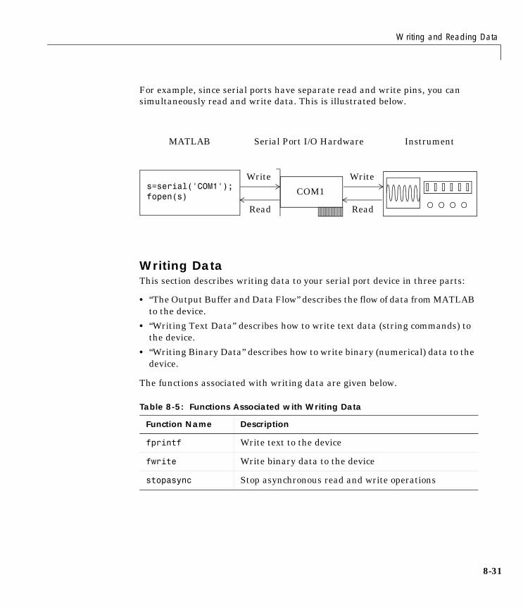
Writing and Reading Data
8-31
For example, since serial ports have separate read and write pins, you can simultaneously read and write data. This is illustrated below.
Writing DataThis section describes writing data to your serial port device in three parts:
• “The Output Buffer and Data Flow” describes the flow of data from MATLAB to the device.
• “Writing Text Data” describes how to write text data (string commands) to the device.
• “Writing Binary Data” describes how to write binary (numerical) data to the device.
The functions associated with writing data are given below.
Table 8-5: Functions Associated with Writing Data
Function Name Description
fprintf Write text to the device
fwrite Write binary data to the device
stopasync Stop asynchronous read and write operations
Serial Port I/O Hardware
s=serial('COM1');fopen(s) COM1
InstrumentMATLAB
Write
Read
Write
Read
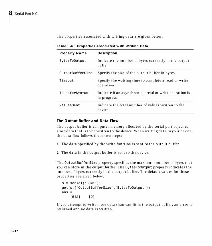
8 Serial Port I/O
8-32
The properties associated with writing data are given below.
The Output Buffer and Data FlowThe output buffer is computer memory allocated by the serial port object to store data that is to be written to the device. When writing data to your device, the data flow follows these two steps:
1 The data specified by the write function is sent to the output buffer.
2 The data in the output buffer is sent to the device.
The OutputBufferSize property specifies the maximum number of bytes that you can store in the output buffer. The BytesToOutput property indicates the number of bytes currently in the output buffer. The default values for these properties are given below.
s = serial('COM1');get(s,{'OutputBufferSize','BytesToOutput'})ans = [512] [0]
If you attempt to write more data than can fit in the output buffer, an error is returned and no data is written.
Table 8-6: Properties Associated with Writing Data
Property Name Description
BytesToOutput Indicate the number of bytes currently in the output buffer
OutputBufferSize Specify the size of the output buffer in bytes
Timeout Specify the waiting time to complete a read or write operation
TransferStatus Indicate if an asynchronous read or write operation is in progress
ValuesSent Indicate the total number of values written to the device
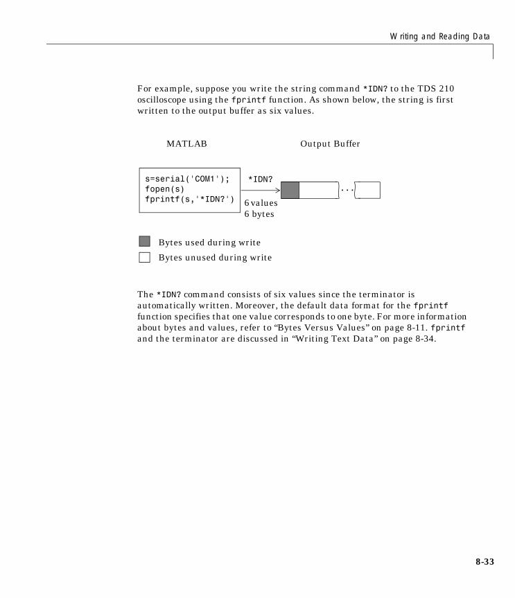
Writing and Reading Data
8-33
For example, suppose you write the string command *IDN? to the TDS 210 oscilloscope using the fprintf function. As shown below, the string is first written to the output buffer as six values.
The *IDN? command consists of six values since the terminator is automatically written. Moreover, the default data format for the fprintf function specifies that one value corresponds to one byte. For more information about bytes and values, refer to “Bytes Versus Values” on page 8-11. fprintf and the terminator are discussed in “Writing Text Data” on page 8-34.
s=serial('COM1');fopen(s)fprintf(s,'*IDN?')
...*IDN?
6 values 6 bytes
MATLAB Output Buffer
Bytes used during write
Bytes unused during write

8 Serial Port I/O
8-34
As shown below, after the string is written to the output buffer, it is then written to the device via the serial port.
Writing Text DataYou use the fprintf function to write text data to the device. For many devices, writing text data means writing string commands that change device settings, prepare the device to return data or status information, and so on.
For example, the Display:Contrast command changes the display contrast of the oscilloscope.
s = serial('COM1');fopen(s)fprintf(s,'Display:Contrast 45')
By default, fprintf writes data using the %s\n format since many serial port devices accept only text-based commands. However, you can specify many other formats as described in the fprintf reference pages.
You can verify the number of values sent to the device with the ValuesSent property.
s.ValuesSentans = 20
COM1...
Output Buffer
Bytes used during write
Bytes unused during write
6 values 6 bytes
Serial Port I/O Hardware Instrument
*IDN?
Writing and Reading Data
8-35
Note that the ValuesSent property value includes the terminator since each occurrence of \n in the command sent to the device is replaced with the Terminator property value.
s.Terminatorans =LF
The default value of Terminator is the line feed character. The terminator required by your device will be described in its documentation.
Synchronous Versus Asynchronous Write Operations. By default, fprintf operates synchronously and will block the MATLAB command line until execution completes. To write text data asynchronously to the device, you must specify async as the last input argument to fprintf.
fprintf(s,'Display:Contrast 45','async')
Asynchronous operations do not block access to the MATLAB command line. Additionally, while an asynchronous write operation is in progress, you can:
• Execute an asynchronous read operation since serial ports have separate pins for reading and writing
• Make use of all supported callback properties
You can determine which asynchronous operations are in progress with the TransferStatus property. If no asynchronous operations are in progress, then TransferStatus is idle.
s.TransferStatusans =idle
Rules for Completing a Write Operation with fprintf. A synchronous or asynchronous write operation using fprintf completes when:
• The specified data is written.
• The time specified by the Timeout property passes.
Additionally, you can stop an asynchronous write operation with the stopasync function.
8 Serial Port I/O
8-36
Writing Binary DataYou use the fwrite function to write binary data to the device. Writing binary data means writing numerical values. A typical application for writing binary data involves writing calibration data to an instrument such as an arbitrary waveform generator.
Note Some serial port devices accept only text-based commands. These commands may use the SCPI language or some other vendor-specific language. Therefore, you may need to use the fprintf function for all write operations.
By default, fwrite translates values using the uchar precision. However, you can specify many other precisions as described in the reference pages for this function.
By default, fwrite operates synchronously. To write binary data asynchronously to the device, you must specify async as the last input argument to fwrite. For more information about synchronous and asynchronous write operations, refer to the “Writing Text Data” on page 8-34. For a description of the rules used by fwrite to complete a write operation, refer to its reference pages.
Reading DataThis section describes reading data from your serial port device in three parts:
• “The Input Buffer and Data Flow” describes the flow of data from the device to MATLAB.
• “Reading Text Data” describes how to read from the device, and format the data as text.
• “Reading Binary Data” describes how to read binary (numerical) data from the device.
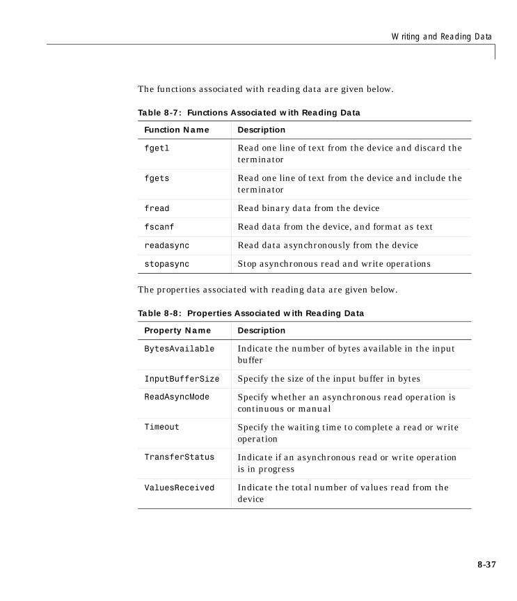
Writing and Reading Data
8-37
The functions associated with reading data are given below.
The properties associated with reading data are given below.
Table 8-7: Functions Associated with Reading Data
Function Name Description
fgetl Read one line of text from the device and discard the terminator
fgets Read one line of text from the device and include the terminator
fread Read binary data from the device
fscanf Read data from the device, and format as text
readasync Read data asynchronously from the device
stopasync Stop asynchronous read and write operations
Table 8-8: Properties Associated with Reading Data
Property Name Description
BytesAvailable Indicate the number of bytes available in the input buffer
InputBufferSize Specify the size of the input buffer in bytes
ReadAsyncMode Specify whether an asynchronous read operation is continuous or manual
Timeout Specify the waiting time to complete a read or write operation
TransferStatus Indicate if an asynchronous read or write operation is in progress
ValuesReceived Indicate the total number of values read from the device
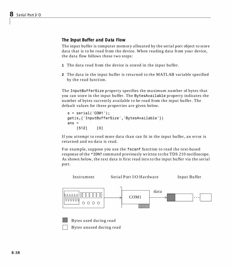
8 Serial Port I/O
8-38
The Input Buffer and Data FlowThe input buffer is computer memory allocated by the serial port object to store data that is to be read from the device. When reading data from your device, the data flow follows these two steps:
1 The data read from the device is stored in the input buffer.
2 The data in the input buffer is returned to the MATLAB variable specified by the read function.
The InputBufferSize property specifies the maximum number of bytes that you can store in the input buffer. The BytesAvailable property indicates the number of bytes currently available to be read from the input buffer. The default values for these properties are given below.
s = serial('COM1');get(s,{'InputBufferSize','BytesAvailable'})ans = [512] [0]
If you attempt to read more data than can fit in the input buffer, an error is returned and no data is read.
For example, suppose you use the fscanf function to read the text-based response of the *IDN? command previously written to the TDS 210 oscilloscope. As shown below, the text data is first read into to the input buffer via the serial port.
COM1 ...
Input Buffer
Bytes used during read
Bytes unused during read
Serial Port I/O HardwareInstrument
data
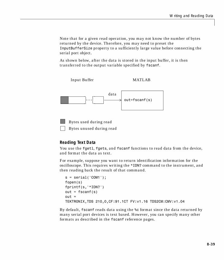
Writing and Reading Data
8-39
Note that for a given read operation, you may not know the number of bytes returned by the device. Therefore, you may need to preset the InputBufferSize property to a sufficiently large value before connecting the serial port object.
As shown below, after the data is stored in the input buffer, it is then transferred to the output variable specified by fscanf.
Reading Text DataYou use the fgetl, fgets, and fscanf functions to read data from the device, and format the data as text.
For example, suppose you want to return identification information for the oscilloscope. This requires writing the *IDN? command to the instrument, and then reading back the result of that command.
s = serial('COM1');fopen(s)fprintf(s,'*IDN?')out = fscanf(s)out =TEKTRONIX,TDS 210,0,CF:91.1CT FV:v1.16 TDS2CM:CMV:v1.04
By default, fscanf reads data using the %c format since the data returned by many serial port devices is text based. However, you can specify many other formats as described in the fscanf reference pages.
out=fscanf(s)...
MATLABInput Buffer
Bytes used during read
Bytes unused during read
data
8 Serial Port I/O
8-40
You can verify the number of values read from the device – including the terminator – with the ValuesReceived property.
s.ValuesReceivedans = 56
Synchronous Versus Asynchronous Read Operations. You specify whether read operations are synchronous or asynchronous with the ReadAsyncMode property. You can configure ReadAsyncMode to continuous or manual.
If ReadAsyncMode is continuous (the default value), the serial port object continuously queries the device to determine if data is available to be read. If data is available, it is asynchronously stored in the input buffer. To transfer the data from the input buffer to MATLAB, you use one of the synchronous (blocking) read functions such as fgetl or fscanf. If data is available in the input buffer, these functions will return quickly.
s.ReadAsyncMode = 'continuous';fprintf(s,'*IDN?')s.BytesAvailableans = 56out = fscanf(s);
If ReadAsyncMode is manual, the serial port object does not continuously query the device to determine if data is available to be read. To read data asynchronously, you use the readasync function.You then use one of the synchronous read functions to transfer data from the input buffer to MATLAB.
s.ReadAsyncMode = 'manual';fprintf(s,'*IDN?')s.BytesAvailableans = 0readasync(s)s.BytesAvailableans = 56out = fscanf(s);
Writing and Reading Data
8-41
Asynchronous operations do not block access to the MATLAB command line. Additionally, while an asynchronous read operation is in progress, you can:
• Execute an asynchronous write operation since serial ports have separate pins for reading and writing
• Make use of all supported callback properties
You can determine which asynchronous operations are in progress with the TransferStatus property. If no asynchronous operations are in progress, then TransferStatus is idle.
s.TransferStatusans =idle
Rules for Completing a Read Operation with fscanf. A read operation with fscanf blocks access to the MATLAB command line until:
• The terminator specified by the Terminator property is read.
• The time specified by the Timeout property passes.
• The specified number of values specified is read.
• The input buffer is filled.
Reading Binary DataYou use the fread function to read binary data from the device. Reading binary data means that you return numerical values to MATLAB.
For example, suppose you want to return the cursor and display settings for the oscilloscope. This requires writing the CURSOR? and DISPLAY? commands to the instrument, and then reading back the results of those commands.
s = serial('COM1');fopen(s)fprintf(s,'CURSOR?')fprintf(s,'DISPLAY?')
Since the default value for the ReadAsyncMode property is continuous, data is asynchronously returned to the input buffer as soon as it is available from the device. You can verify the number of values read with the BytesAvailable property.
8 Serial Port I/O
8-42
s.BytesAvailableans = 69
You can return the data to MATLAB using any of the synchronous read functions. However, if you use fgetl, fgets, or fscanf, then you must issue the function twice since there are two terminators stored in the input buffer. If you use fread, then you can return all the data to MATLAB in one function call.
out = fread(s,69);
By default, fread returns numerical values in double precision arrays. However, you can specify many other precisions as described in the fread reference pages. You can convert the numerical data to text using MATLAB’s char function.
val = char(out)'val =HBARS;CH1;SECONDS;-1.0E-3;1.0E-3;VOLTS;-6.56E-1;6.24E-1YT;DOTS;0;45
For more information about synchronous and asynchronous read operations, refer to “Reading Text Data” on page 8-39. For a description of the rules used by fread to complete a read operation, refer to its reference pages.
Example: Writing and Reading Text DataThis example illustrates how to communicate with a serial port instrument by writing and reading text data.
The instrument is a Tektronix TDS 210 two-channel oscilloscope connected to the serial port COM1. Therefore, many of the commands given below are specific to this instrument. A sine wave is input into channel 2 of the oscilloscope, and your job is to measure the peak-to-peak voltage of the input signal.
1. Create a serial port object – Create the serial port object s associated with serial port COM1.
s = serial('COM1');
2. Connect to the device – Connect s to the oscilloscope. Since the default value for the ReadAsyncMode property is continuous, data is asynchronously returned to the input buffer as soon as it is available from the instrument.
Writing and Reading Data
8-43
fopen(s)
3. Write and read data – Write the *IDN? command to the instrument using fprintf, and then read back the result of the command using fscanf.
fprintf(s,'*IDN?')idn = fscanf(s)idn =TEKTRONIX,TDS 210,0,CF:91.1CT FV:v1.16 TDS2CM:CMV:v1.04
You need to determine the measurement source. Possible measurement sources include channel 1 and channel 2 of the oscilloscope.
fprintf(s,'MEASUREMENT:IMMED:SOURCE?')source = fscanf(s)source =CH1
The scope is configured to return a measurement from channel 1. Since the input signal is connected to channel 2, you must configure the instrument to return a measurement from this channel.
fprintf(s,'MEASUREMENT:IMMED:SOURCE CH2')fprintf(s,'MEASUREMENT:IMMED:SOURCE?')source = fscanf(s)source =CH2
You can now configure the scope to return the peak-to-peak voltage, and then request the value of this measurement.
fprintf(s,'MEASUREMENT:MEAS1:TYPE PK2PK')fprintf(s,'MEASUREMENT:MEAS1:VALUE?')
Transfer data from the input buffer to MATLAB using fscanf.
ptop = fscanf(s,'%g')ptop =2.0199999809E0
4. Disconnect and clean up – When you no longer need s, you should disconnect it from the instrument, and remove it from memory and from the MATLAB workspace.
fclose(s)
8 Serial Port I/O
8-44
delete(s)clear s
Example: Parsing Input Data Using strreadThis example illustrates how to use the strread function to parse and format data that you read from a device. strread is particularly useful when you want to parse a string into one or more variables, where each variable has its own specified format.
The instrument is a Tektronix TDS 210 two-channel oscilloscope connected to the serial port COM1.
1. Create a serial port object – Create the serial port object s associated with serial port COM1.
s = serial('COM1');
2. Connect to the device – Connect s to the oscilloscope. Since the default value for the ReadAsyncMode property is continuous, data is asynchronously returned to the input buffer as soon as it is available from the instrument.
fopen(s)
3. Write and read data – Write the RS232? command to the instrument using fprintf, and then read back the result of the command using fscanf. RS232? queries the RS-232 settings and returns the baud rate, the software flow control setting, the hardware flow control setting, the parity type, and the terminator.
fprintf(s,'RS232?')data = fscanf(s)data =9600;0;0;NONE;LF
Use the strread function to parse and format the data variable into five new variables.
[br,sfc,hfc,par,tm] = strread(data,'%d%d%d%s%s','delimiter',';')
br = 9600sfc = 0
Writing and Reading Data
8-45
hfc = 0par = 'NONE'tm = 'LF'
4. Disconnect and clean up – When you no longer need s, you should disconnect it from the instrument, and remove it from memory and from the MATLAB workspace.
fclose(s)delete(s)clear s
Example: Reading Binary DataThis example illustrates how you can download the TDS 210 oscilloscope screen display to MATLAB. The screen display data is transferred and saved to disk using the Windows bitmap format. This data provides a permanent record of your work, and is an easy way to document important signal and scope parameters.
Since the amount of data transferred is expected to be fairly large, it is asynchronously returned to the input buffer as soon as it is available from the instrument. This allows you to perform other tasks as the transfer progresses. Additionally, the scope is configured to its highest baud rate of 19,200.
1. Create a serial port object – Create the serial port object s associated with serial port COM1.
s = serial('COM1');
2. Configure property values – Configure the input buffer to accept a reasonably large number of bytes, and configure the baud rate to the highest value supported by the scope.
s.InputBufferSize = 50000;s.BaudRate = 19200;
3. Connect to the device – Connect s to the oscilloscope. Since the default value for the ReadAsyncMode property is continuous, data is asynchronously returned to the input buffer as soon as it is available from the instrument.
8 Serial Port I/O
8-46
fopen(s)
4. Write and read data – Configure the scope to transfer the screen display as a bitmap.
fprintf(s,'HARDCOPY:PORT RS232')fprintf(s,'HARDCOPY:FORMAT BMP')fprintf(s,'HARDCOPY START')
Wait until all the data is sent to the input buffer, and then transfer the data to the MATLAB workspace as unsigned 8-bit integers.
out = fread(s,s.BytesAvailable,'uint8');
5. Disconnect and clean up – When you no longer need s, you should disconnect it from the instrument, and remove it from memory and from the MATLAB workspace.
fclose(s)delete(s)clear s
Viewing the Bitmap DataTo view the bitmap data, you should follow these steps:
1 Open a disk file.
2 Write the data to the disk file.
3 Close the disk file.
4 Read the data into MATLAB using the imread function.
5 Scale and display the data using the imagesc function.
Note that the file I/O versions of the fopen, fwrite, and fclose functions are used.
fid = fopen('test1.bmp','w');fwrite(fid,out,'uint8');fclose(fid)a = imread('test1.bmp','bmp');imagesc(a)

Writing and Reading Data
8-47
Since the scope returns the screen display data using only two colors, an appropriate colormap is selected.
mymap = [0 0 0; 1 1 1];colormap(mymap)
The resulting bitmap image is shown below.
8 Serial Port I/O
8-48
Events and CallbacksYou can enhance the power and flexibility of your serial port application by using events. An event occurs after a condition is met and may result in one or more callbacks.
While the serial port object is connected to the device, you can use events to display a message, display data, analyze data, and so on. Callbacks are controlled through callback properties and callback functions. All event types have an associated callback property. Callback functions are M-file functions that you construct to suit your specific application needs.
You execute a callback when a particular event occurs by specifying the name of the M-file callback function as the value for the associated callback property.
Example: Introduction to Events and CallbacksThis example uses the M-file callback function instrcallback to display a message to the command line when a bytes-available event occurs. The event is generated when the terminator is read.
s = serial('COM1');fopen(s)s.BytesAvailableFcnMode = 'terminator';s.BytesAvailableFcn = @instrcallback;fprintf(s,'*IDN?')out = fscanf(s);
The resulting display from instrcallback is shown below.
BytesAvailable event occurred at 17:01:29 for the object: Serial-COM1.
End the serial port session.
fclose(s)delete(s)clear s
You can use the type command to display instrcallback at the command line.
Events and Callbacks
8-49
Event Types and Callback PropertiesThe serial port event types and associated callback properties are described below.
Break-Interrupt Event. A break-interrupt event is generated immediately after a break interrupt is generated by the serial port. The serial port generates a break interrupt when the received data has been in an inactive state longer than the transmission time for one character.
This event executes the callback function specified for the BreakInterruptFcn property. It can be generated for both synchronous and asynchronous read and write operations.
Bytes-Available Event. A bytes-available event is generated immediately after a predetermined number of bytes are available in the input buffer or a terminator is read, as determined by the BytesAvailableFcnMode property.
If BytesAvailableFcnMode is byte, the bytes-available event executes the callback function specified for the BytesAvailableFcn property every time the number of bytes specified by BytesAvailableFcnCount is stored in the input
Table 8-9: Event Types and Callback Properties
Event Type Associated Properties
Break interrupt BreakInterruptFcn
Bytes available BytesAvailableFcn
BytesAvailableFcnCount
BytesAvailableFcnMode
Error ErrorFcn
Output empty OutputEmptyFcn
Pin status PinStatusFcn
Timer TimerFcn
TimerPeriod
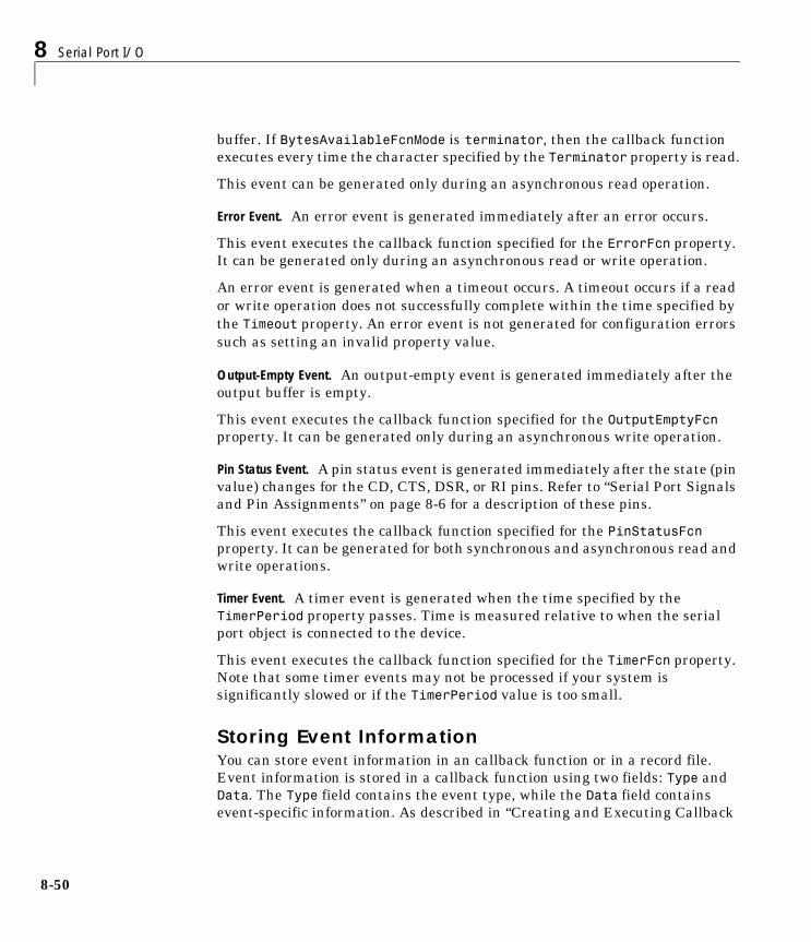
8 Serial Port I/O
8-50
buffer. If BytesAvailableFcnMode is terminator, then the callback function executes every time the character specified by the Terminator property is read.
This event can be generated only during an asynchronous read operation.
Error Event. An error event is generated immediately after an error occurs.
This event executes the callback function specified for the ErrorFcn property. It can be generated only during an asynchronous read or write operation.
An error event is generated when a timeout occurs. A timeout occurs if a read or write operation does not successfully complete within the time specified by the Timeout property. An error event is not generated for configuration errors such as setting an invalid property value.
Output-Empty Event. An output-empty event is generated immediately after the output buffer is empty.
This event executes the callback function specified for the OutputEmptyFcn property. It can be generated only during an asynchronous write operation.
Pin Status Event. A pin status event is generated immediately after the state (pin value) changes for the CD, CTS, DSR, or RI pins. Refer to “Serial Port Signals and Pin Assignments” on page 8-6 for a description of these pins.
This event executes the callback function specified for the PinStatusFcn property. It can be generated for both synchronous and asynchronous read and write operations.
Timer Event. A timer event is generated when the time specified by the TimerPeriod property passes. Time is measured relative to when the serial port object is connected to the device.
This event executes the callback function specified for the TimerFcn property. Note that some timer events may not be processed if your system is significantly slowed or if the TimerPeriod value is too small.
Storing Event InformationYou can store event information in an callback function or in a record file. Event information is stored in a callback function using two fields: Type and Data. The Type field contains the event type, while the Data field contains event-specific information. As described in “Creating and Executing Callback
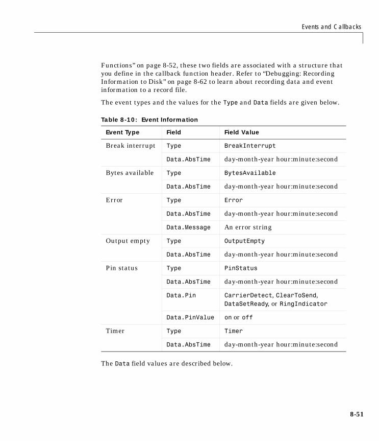
Events and Callbacks
8-51
Functions” on page 8-52, these two fields are associated with a structure that you define in the callback function header. Refer to “Debugging: Recording Information to Disk” on page 8-62 to learn about recording data and event information to a record file.
The event types and the values for the Type and Data fields are given below.
The Data field values are described below.
Table 8-10: Event Information
Event Type Field Field Value
Break interrupt Type BreakInterrupt
Data.AbsTime day-month-year hour:minute:second
Bytes available Type BytesAvailable
Data.AbsTime day-month-year hour:minute:second
Error Type Error
Data.AbsTime day-month-year hour:minute:second
Data.Message An error string
Output empty Type OutputEmpty
Data.AbsTime day-month-year hour:minute:second
Pin status Type PinStatus
Data.AbsTime day-month-year hour:minute:second
Data.Pin CarrierDetect, ClearToSend, DataSetReady, or RingIndicator
Data.PinValue on or off
Timer Type Timer
Data.AbsTime day-month-year hour:minute:second
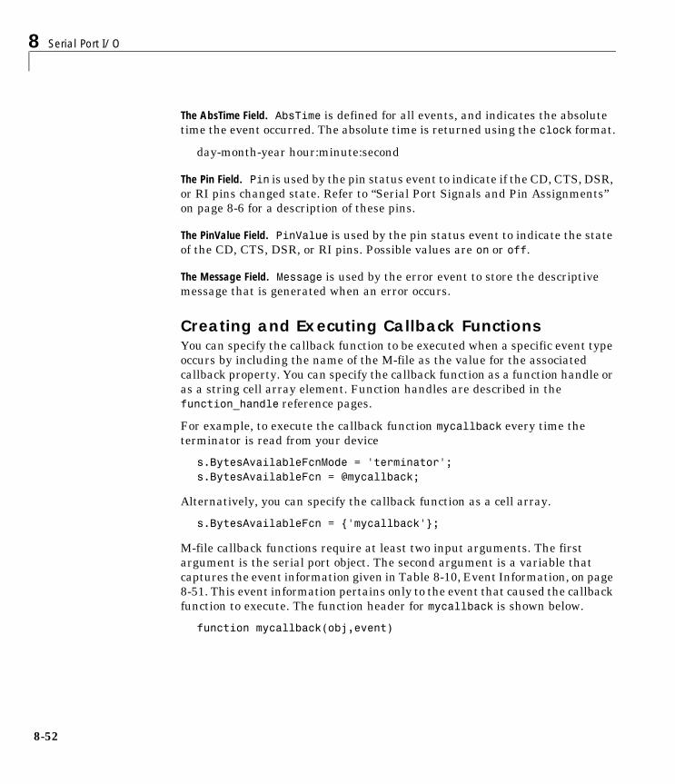
8 Serial Port I/O
8-52
The AbsTime Field. AbsTime is defined for all events, and indicates the absolute time the event occurred. The absolute time is returned using the clock format.
day-month-year hour:minute:second
The Pin Field. Pin is used by the pin status event to indicate if the CD, CTS, DSR, or RI pins changed state. Refer to “Serial Port Signals and Pin Assignments” on page 8-6 for a description of these pins.
The PinValue Field. PinValue is used by the pin status event to indicate the state of the CD, CTS, DSR, or RI pins. Possible values are on or off.
The Message Field. Message is used by the error event to store the descriptive message that is generated when an error occurs.
Creating and Executing Callback FunctionsYou can specify the callback function to be executed when a specific event type occurs by including the name of the M-file as the value for the associated callback property. You can specify the callback function as a function handle or as a string cell array element. Function handles are described in the function_handle reference pages.
For example, to execute the callback function mycallback every time the terminator is read from your device
s.BytesAvailableFcnMode = 'terminator';s.BytesAvailableFcn = @mycallback;
Alternatively, you can specify the callback function as a cell array.
s.BytesAvailableFcn = {'mycallback'};
M-file callback functions require at least two input arguments. The first argument is the serial port object. The second argument is a variable that captures the event information given in Table 8-10, Event Information, on page 8-51. This event information pertains only to the event that caused the callback function to execute. The function header for mycallback is shown below.
function mycallback(obj,event)
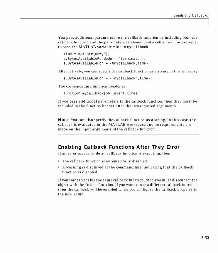
Events and Callbacks
8-53
You pass additional parameters to the callback function by including both the callback function and the parameters as elements of a cell array. For example, to pass the MATLAB variable time to mycallback
time = datestr(now,0);s.BytesAvailableFcnMode = 'terminator';s.BytesAvailableFcn = {@mycallback,time};
Alternatively, you can specify the callback function as a string in the cell array.
s.BytesAvailableFcn = {'mycallback',time};
The corresponding function header is
function mycallback(obj,event,time)
If you pass additional parameters to the callback function, then they must be included in the function header after the two required arguments.
Note You can also specify the callback function as a string. In this case, the callback is evaluated in the MATLAB workspace and no requirements are made on the input arguments of the callback function.
Enabling Callback Functions After They ErrorIf an error occurs while an callback function is executing, then:
• The callback function is automatically disabled.
• A warning is displayed at the command line, indicating that the callback function is disabled.
If you want to enable the same callback function, then you must disconnect the object with the fclose function. If you want to use a different callback function, then the callback will be enabled when you configure the callback property to the new value.
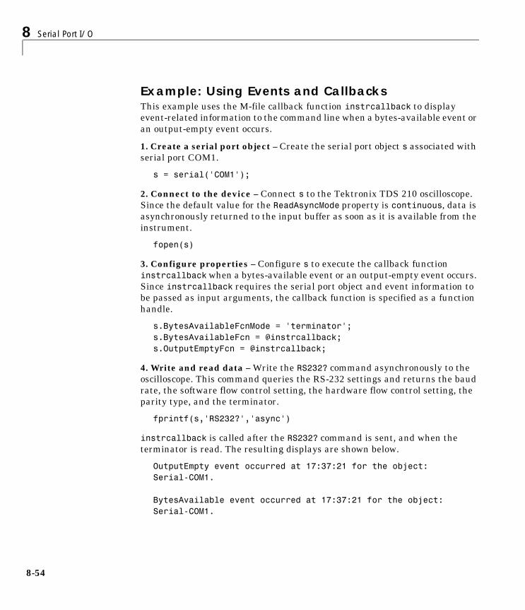
8 Serial Port I/O
8-54
Example: Using Events and CallbacksThis example uses the M-file callback function instrcallback to display event-related information to the command line when a bytes-available event or an output-empty event occurs.
1. Create a serial port object – Create the serial port object s associated with serial port COM1.
s = serial('COM1');
2. Connect to the device – Connect s to the Tektronix TDS 210 oscilloscope. Since the default value for the ReadAsyncMode property is continuous, data is asynchronously returned to the input buffer as soon as it is available from the instrument.
fopen(s)
3. Configure properties – Configure s to execute the callback function instrcallback when a bytes-available event or an output-empty event occurs. Since instrcallback requires the serial port object and event information to be passed as input arguments, the callback function is specified as a function handle.
s.BytesAvailableFcnMode = 'terminator';s.BytesAvailableFcn = @instrcallback;s.OutputEmptyFcn = @instrcallback;
4. Write and read data – Write the RS232? command asynchronously to the oscilloscope. This command queries the RS-232 settings and returns the baud rate, the software flow control setting, the hardware flow control setting, the parity type, and the terminator.
fprintf(s,'RS232?','async')
instrcallback is called after the RS232? command is sent, and when the terminator is read. The resulting displays are shown below.
OutputEmpty event occurred at 17:37:21 for the object: Serial-COM1.
BytesAvailable event occurred at 17:37:21 for the object: Serial-COM1.
Events and Callbacks
8-55
Read the data from the input buffer.
out = fscanf(s)out =9600;0;0;NONE;LF
5. Disconnect and clean up – When you no longer need s, you should disconnect it from the instrument, and remove it from memory and from the MATLAB workspace.
fclose(s)delete(s)clear s
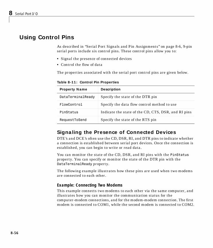
8 Serial Port I/O
8-56
Using Control PinsAs described in “Serial Port Signals and Pin Assignments” on page 8-6, 9-pin serial ports include six control pins. These control pins allow you to:
• Signal the presence of connected devices
• Control the flow of data
The properties associated with the serial port control pins are given below.
Signaling the Presence of Connected DevicesDTE’s and DCE’s often use the CD, DSR, RI, and DTR pins to indicate whether a connection is established between serial port devices. Once the connection is established, you can begin to write or read data.
You can monitor the state of the CD, DSR, and RI pins with the PinStatus property. You can specify or monitor the state of the DTR pin with the DataTerminalReady property.
The following example illustrates how these pins are used when two modems are connected to each other.
Example: Connecting Two ModemsThis example connects two modems to each other via the same computer, and illustrates how you can monitor the communication status for the computer-modem connections, and for the modem-modem connection. The first modem is connected to COM1, while the second modem is connected to COM2.
Table 8-11: Control Pin Properties
Property Name Description
DataTerminalReady Specify the state of the DTR pin
FlowControl Specify the data flow control method to use
PinStatus Indicate the state of the CD, CTS, DSR, and RI pins
RequestToSend Specify the state of the RTS pin
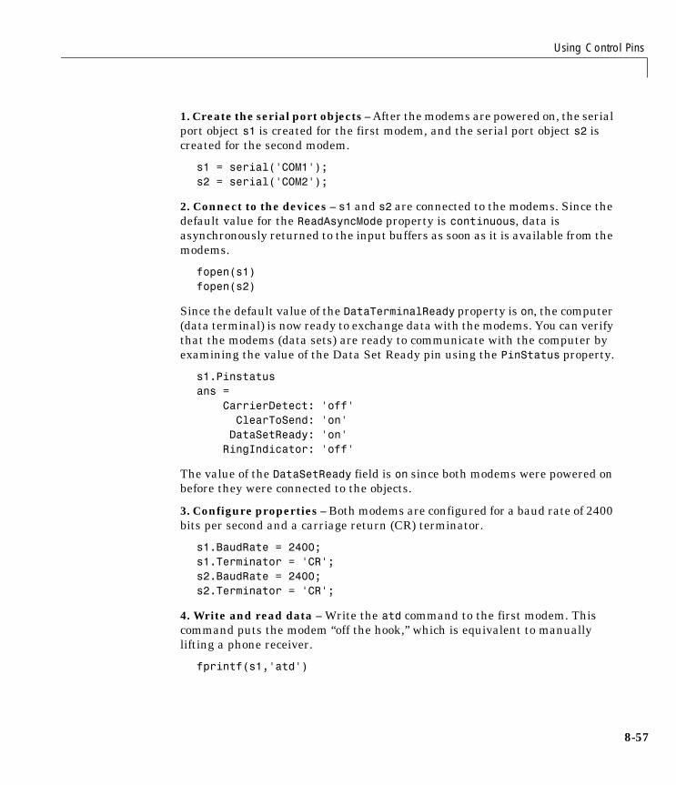
Using Control Pins
8-57
1. Create the serial port objects – After the modems are powered on, the serial port object s1 is created for the first modem, and the serial port object s2 is created for the second modem.
s1 = serial('COM1');s2 = serial('COM2');
2. Connect to the devices – s1 and s2 are connected to the modems. Since the default value for the ReadAsyncMode property is continuous, data is asynchronously returned to the input buffers as soon as it is available from the modems.
fopen(s1)fopen(s2)
Since the default value of the DataTerminalReady property is on, the computer (data terminal) is now ready to exchange data with the modems. You can verify that the modems (data sets) are ready to communicate with the computer by examining the value of the Data Set Ready pin using the PinStatus property.
s1.Pinstatusans = CarrierDetect: 'off' ClearToSend: 'on' DataSetReady: 'on' RingIndicator: 'off'
The value of the DataSetReady field is on since both modems were powered on before they were connected to the objects.
3. Configure properties – Both modems are configured for a baud rate of 2400 bits per second and a carriage return (CR) terminator.
s1.BaudRate = 2400;s1.Terminator = 'CR';s2.BaudRate = 2400;s2.Terminator = 'CR';
4. Write and read data – Write the atd command to the first modem. This command puts the modem “off the hook,” which is equivalent to manually lifting a phone receiver.
fprintf(s1,'atd')
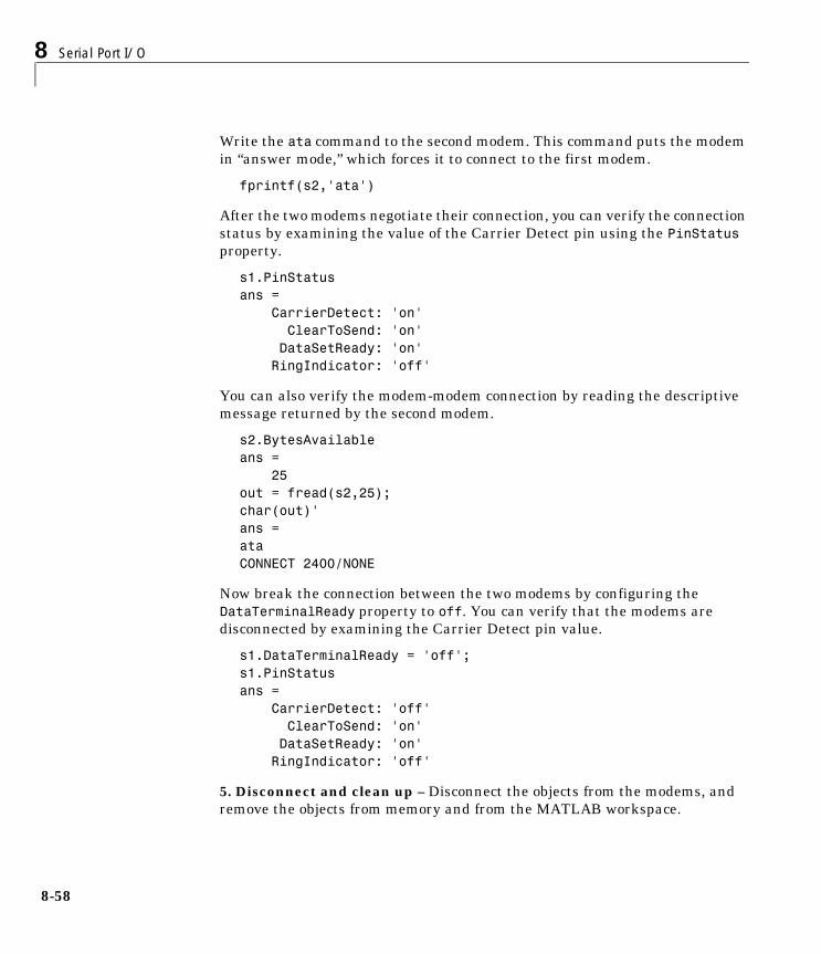
8 Serial Port I/O
8-58
Write the ata command to the second modem. This command puts the modem in “answer mode,” which forces it to connect to the first modem.
fprintf(s2,'ata')
After the two modems negotiate their connection, you can verify the connection status by examining the value of the Carrier Detect pin using the PinStatus property.
s1.PinStatusans = CarrierDetect: 'on' ClearToSend: 'on' DataSetReady: 'on' RingIndicator: 'off'
You can also verify the modem-modem connection by reading the descriptive message returned by the second modem.
s2.BytesAvailableans = 25out = fread(s2,25);char(out)'ans =ataCONNECT 2400/NONE
Now break the connection between the two modems by configuring the DataTerminalReady property to off. You can verify that the modems are disconnected by examining the Carrier Detect pin value.
s1.DataTerminalReady = 'off';s1.PinStatusans = CarrierDetect: 'off' ClearToSend: 'on' DataSetReady: 'on' RingIndicator: 'off'
5. Disconnect and clean up – Disconnect the objects from the modems, and remove the objects from memory and from the MATLAB workspace.
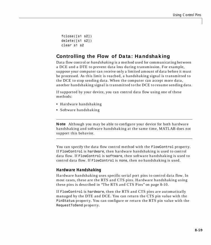
Using Control Pins
8-59
fclose([s1 s2])delete([s1 s2])clear s1 s2
Controlling the Flow of Data: HandshakingData flow control or handshaking is a method used for communicating between a DCE and a DTE to prevent data loss during transmission. For example, suppose your computer can receive only a limited amount of data before it must be processed. As this limit is reached, a handshaking signal is transmitted to the DCE to stop sending data. When the computer can accept more data, another handshaking signal is transmitted to the DCE to resume sending data.
If supported by your device, you can control data flow using one of these methods:
• Hardware handshaking
• Software handshaking
Note Although you may be able to configure your device for both hardware handshaking and software handshaking at the same time, MATLAB does not support this behavior.
You can specify the data flow control method with the FlowControl property. If FlowControl is hardware, then hardware handshaking is used to control data flow. If FlowControl is software, then software handshaking is used to control data flow. If FlowControl is none, then no handshaking is used.
Hardware HandshakingHardware handshaking uses specific serial port pins to control data flow. In most cases, these are the RTS and CTS pins. Hardware handshaking using these pins is described in “The RTS and CTS Pins” on page 8-10.
If FlowControl is hardware, then the RTS and CTS pins are automatically managed by the DTE and DCE. You can return the CTS pin value with the PinStatus property. You can configure or return the RTS pin value with the RequestToSend property.
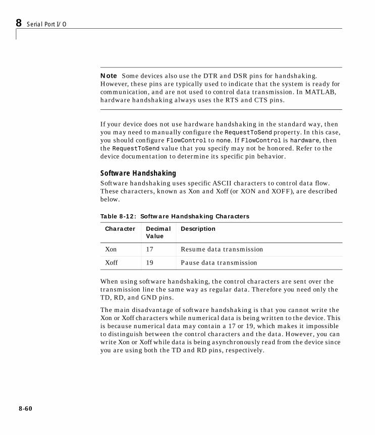
8 Serial Port I/O
8-60
Note Some devices also use the DTR and DSR pins for handshaking. However, these pins are typically used to indicate that the system is ready for communication, and are not used to control data transmission. In MATLAB, hardware handshaking always uses the RTS and CTS pins.
If your device does not use hardware handshaking in the standard way, then you may need to manually configure the RequestToSend property. In this case, you should configure FlowControl to none. If FlowControl is hardware, then the RequestToSend value that you specify may not be honored. Refer to the device documentation to determine its specific pin behavior.
Software HandshakingSoftware handshaking uses specific ASCII characters to control data flow. These characters, known as Xon and Xoff (or XON and XOFF), are described below.
When using software handshaking, the control characters are sent over the transmission line the same way as regular data. Therefore you need only the TD, RD, and GND pins.
The main disadvantage of software handshaking is that you cannot write the Xon or Xoff characters while numerical data is being written to the device. This is because numerical data may contain a 17 or 19, which makes it impossible to distinguish between the control characters and the data. However, you can write Xon or Xoff while data is being asynchronously read from the device since you are using both the TD and RD pins, respectively.
Table 8-12: Software Handshaking Characters
Character Decimal Value
Description
Xon 17 Resume data transmission
Xoff 19 Pause data transmission
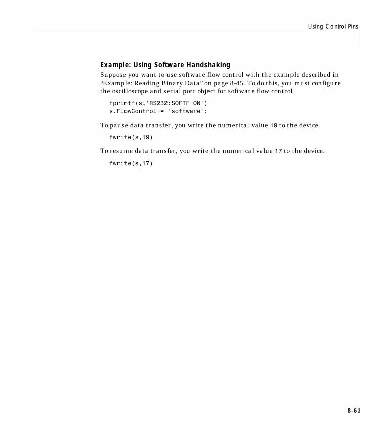
Using Control Pins
8-61
Example: Using Software HandshakingSuppose you want to use software flow control with the example described in “Example: Reading Binary Data” on page 8-45. To do this, you must configure the oscilloscope and serial port object for software flow control.
fprintf(s,'RS232:SOFTF ON')s.FlowControl = 'software';
To pause data transfer, you write the numerical value 19 to the device.
fwrite(s,19)
To resume data transfer, you write the numerical value 17 to the device.
fwrite(s,17)
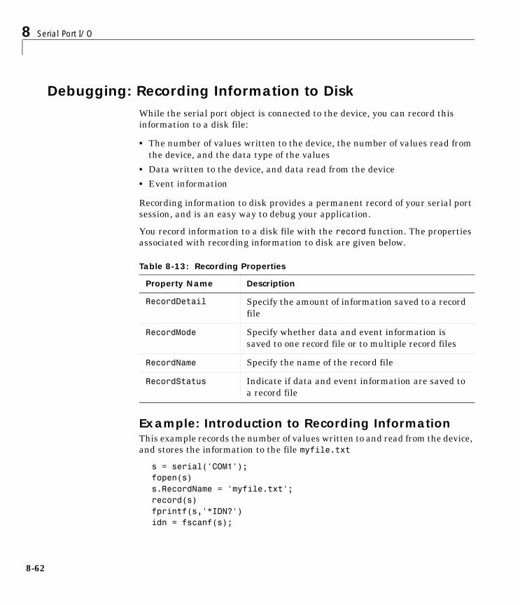
8 Serial Port I/O
8-62
Debugging: Recording Information to DiskWhile the serial port object is connected to the device, you can record this information to a disk file:
• The number of values written to the device, the number of values read from the device, and the data type of the values
• Data written to the device, and data read from the device
• Event information
Recording information to disk provides a permanent record of your serial port session, and is an easy way to debug your application.
You record information to a disk file with the record function. The properties associated with recording information to disk are given below.
Example: Introduction to Recording InformationThis example records the number of values written to and read from the device, and stores the information to the file myfile.txt
s = serial('COM1');fopen(s)s.RecordName = 'myfile.txt';record(s)fprintf(s,'*IDN?')idn = fscanf(s);
Table 8-13: Recording Properties
Property Name Description
RecordDetail Specify the amount of information saved to a record file
RecordMode Specify whether data and event information is saved to one record file or to multiple record files
RecordName Specify the name of the record file
RecordStatus Indicate if data and event information are saved to a record file
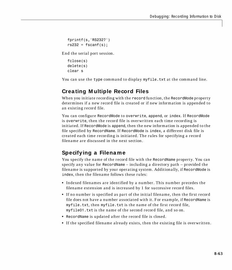
Debugging: Recording Information to Disk
8-63
fprintf(s,'RS232?')rs232 = fscanf(s);
End the serial port session.
fclose(s)delete(s)clear s
You can use the type command to display myfile.txt at the command line.
Creating Multiple Record FilesWhen you initiate recording with the record function, the RecordMode property determines if a new record file is created or if new information is appended to an existing record file.
You can configure RecordMode to overwrite, append, or index. If RecordMode is overwrite, then the record file is overwritten each time recording is initiated. If RecordMode is append, then the new information is appended to the file specified by RecordName. If RecordMode is index, a different disk file is created each time recording is initiated. The rules for specifying a record filename are discussed in the next section.
Specifying a FilenameYou specify the name of the record file with the RecordName property. You can specify any value for RecordName – including a directory path – provided the filename is supported by your operating system. Additionally, if RecordMode is index, then the filename follows these rules:
• Indexed filenames are identified by a number. This number precedes the filename extension and is increased by 1 for successive record files.
• If no number is specified as part of the initial filename, then the first record file does not have a number associated with it. For example, if RecordName is myfile.txt, then myfile.txt is the name of the first record file, myfile01.txt is the name of the second record file, and so on.
• RecordName is updated after the record file is closed.
• If the specified filename already exists, then the existing file is overwritten.
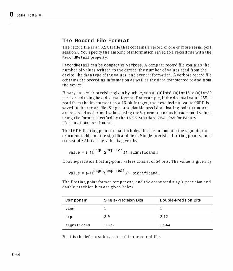
8 Serial Port I/O
8-64
The Record File FormatThe record file is an ASCII file that contains a record of one or more serial port sessions. You specify the amount of information saved to a record file with the RecordDetail property.
RecordDetail can be compact or verbose. A compact record file contains the number of values written to the device, the number of values read from the device, the data type of the values, and event information. A verbose record file contains the preceding information as well as the data transferred to and from the device.
Binary data with precision given by uchar, schar, (u)int8, (u)int16 or (u)int32 is recorded using hexadecimal format. For example, if the decimal value 255 is read from the instrument as a 16-bit integer, the hexadecimal value 00FF is saved in the record file. Single- and double-precision floating-point numbers are recorded as decimal values using the %g format, and as hexadecimal values using the format specified by the IEEE Standard 754-1985 for Binary Floating-Point Arithmetic.
The IEEE floating-point format includes three components: the sign bit, the exponent field, and the significand field. Single-precision floating-point values consist of 32 bits. The value is given by
Double-precision floating-point values consist of 64 bits. The value is given by
The floating-point format component, and the associated single-precision and double-precision bits are given below.
Bit 1 is the left-most bit as stored in the record file.
Component Single-Precision Bits Double-Precision Bits
sign 1 1
exp 2-9 2-12
significand 10-32 13-64
value 1–( )sign 2exp-127( ) 1.significand( )=
value 1–( )sign 2exp-1023( ) 1.significand( )=
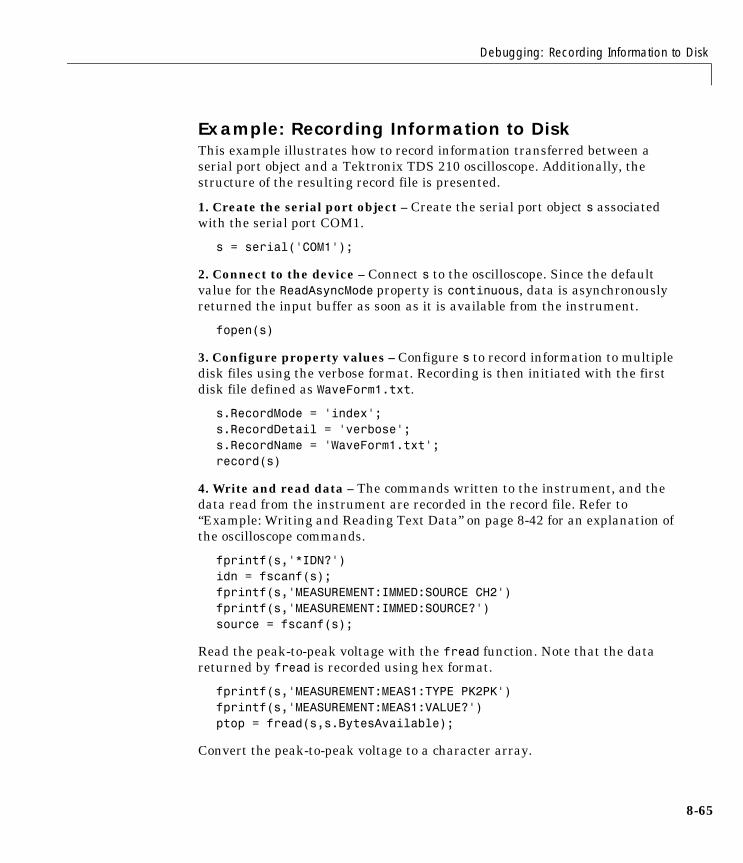
Debugging: Recording Information to Disk
8-65
Example: Recording Information to DiskThis example illustrates how to record information transferred between a serial port object and a Tektronix TDS 210 oscilloscope. Additionally, the structure of the resulting record file is presented.
1. Create the serial port object – Create the serial port object s associated with the serial port COM1.
s = serial('COM1');
2. Connect to the device – Connect s to the oscilloscope. Since the default value for the ReadAsyncMode property is continuous, data is asynchronously returned the input buffer as soon as it is available from the instrument.
fopen(s)
3. Configure property values – Configure s to record information to multiple disk files using the verbose format. Recording is then initiated with the first disk file defined as WaveForm1.txt.
s.RecordMode = 'index';s.RecordDetail = 'verbose';s.RecordName = 'WaveForm1.txt';record(s)
4. Write and read data – The commands written to the instrument, and the data read from the instrument are recorded in the record file. Refer to “Example: Writing and Reading Text Data” on page 8-42 for an explanation of the oscilloscope commands.
fprintf(s,'*IDN?')idn = fscanf(s);fprintf(s,'MEASUREMENT:IMMED:SOURCE CH2')fprintf(s,'MEASUREMENT:IMMED:SOURCE?')source = fscanf(s);
Read the peak-to-peak voltage with the fread function. Note that the data returned by fread is recorded using hex format.
fprintf(s,'MEASUREMENT:MEAS1:TYPE PK2PK')fprintf(s,'MEASUREMENT:MEAS1:VALUE?')ptop = fread(s,s.BytesAvailable);
Convert the peak-to-peak voltage to a character array.
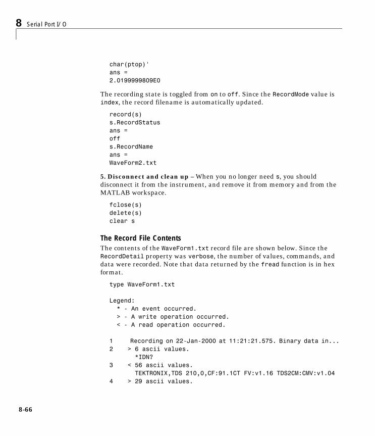
8 Serial Port I/O
8-66
char(ptop)'ans =2.0199999809E0
The recording state is toggled from on to off. Since the RecordMode value is index, the record filename is automatically updated.
record(s)s.RecordStatusans =offs.RecordNameans =WaveForm2.txt
5. Disconnect and clean up – When you no longer need s, you should disconnect it from the instrument, and remove it from memory and from the MATLAB workspace.
fclose(s)delete(s)clear s
The Record File ContentsThe contents of the WaveForm1.txt record file are shown below. Since the RecordDetail property was verbose, the number of values, commands, and data were recorded. Note that data returned by the fread function is in hex format.
type WaveForm1.txt
Legend: * - An event occurred. > - A write operation occurred. < - A read operation occurred. 1 Recording on 22-Jan-2000 at 11:21:21.575. Binary data in... 2 > 6 ascii values. *IDN?3 < 56 ascii values.
TEKTRONIX,TDS 210,0,CF:91.1CT FV:v1.16 TDS2CM:CMV:v1.044 > 29 ascii values.
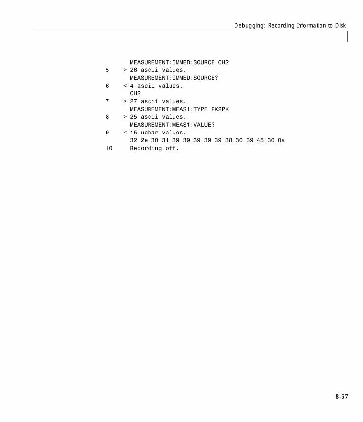
Debugging: Recording Information to Disk
8-67
MEASUREMENT:IMMED:SOURCE CH25 > 26 ascii values. MEASUREMENT:IMMED:SOURCE?6 < 4 ascii values. CH27 > 27 ascii values. MEASUREMENT:MEAS1:TYPE PK2PK8 > 25 ascii values. MEASUREMENT:MEAS1:VALUE?9 < 15 uchar values. 32 2e 30 31 39 39 39 39 39 38 30 39 45 30 0a 10 Recording off.
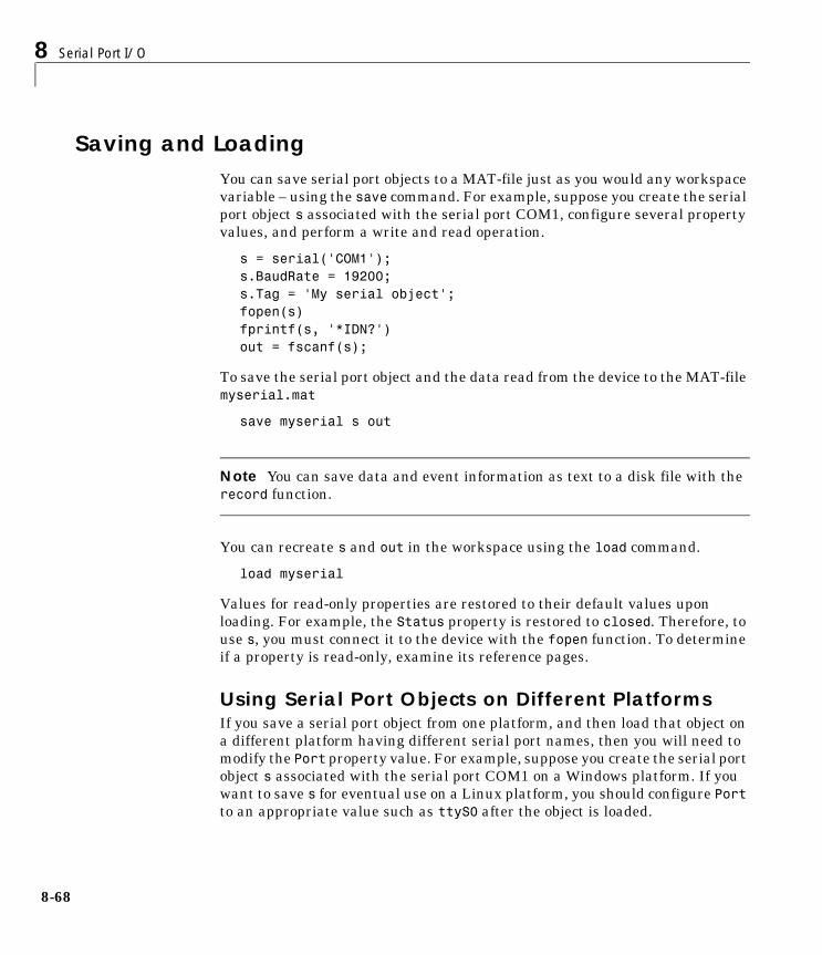
8 Serial Port I/O
8-68
Saving and LoadingYou can save serial port objects to a MAT-file just as you would any workspace variable – using the save command. For example, suppose you create the serial port object s associated with the serial port COM1, configure several property values, and perform a write and read operation.
s = serial('COM1');s.BaudRate = 19200;s.Tag = 'My serial object';fopen(s)fprintf(s, '*IDN?')out = fscanf(s);
To save the serial port object and the data read from the device to the MAT-file myserial.mat
save myserial s out
Note You can save data and event information as text to a disk file with the record function.
You can recreate s and out in the workspace using the load command.
load myserial
Values for read-only properties are restored to their default values upon loading. For example, the Status property is restored to closed. Therefore, to use s, you must connect it to the device with the fopen function. To determine if a property is read-only, examine its reference pages.
Using Serial Port Objects on Different PlatformsIf you save a serial port object from one platform, and then load that object on a different platform having different serial port names, then you will need to modify the Port property value. For example, suppose you create the serial port object s associated with the serial port COM1 on a Windows platform. If you want to save s for eventual use on a Linux platform, you should configure Port to an appropriate value such as ttyS0 after the object is loaded.
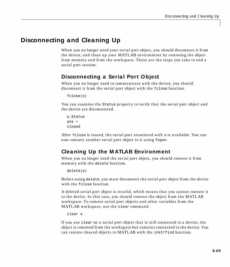
Disconnecting and Cleaning Up
8-69
Disconnecting and Cleaning UpWhen you no longer need your serial port object, you should disconnect it from the device, and clean up your MATLAB environment by removing the object from memory and from the workspace. These are the steps you take to end a serial port session.
Disconnecting a Serial Port ObjectWhen you no longer need to communicate with the device, you should disconnect it from the serial port object with the fclose function.
fclose(s)
You can examine the Status property to verify that the serial port object and the device are disconnected.
s.Statusans =closed
After fclose is issued, the serial port associated with s is available. You can now connect another serial port object to it using fopen.
Cleaning Up the MATLAB EnvironmentWhen you no longer need the serial port object, you should remove it from memory with the delete function.
delete(s)
Before using delete, you must disconnect the serial port object from the device with the fclose function.
A deleted serial port object is invalid, which means that you cannot connect it to the device. In this case, you should remove the object from the MATLAB workspace. To remove serial port objects and other variables from the MATLAB workspace, use the clear command.
clear s
If you use clear on a serial port object that is still connected to a device, the object is removed from the workspace but remains connected to the device. You can restore cleared objects to MATLAB with the instrfind function.
8 Serial Port I/O
8-70
Property ReferenceThis section includes information to help you learn about serial port properties. The information is organized using these topics:
• “The Property Reference Page Format” describes the organization of the property reference pages.
• “Serial Port Object Properties” summarizes the properties using several categories based on how they are used. Following this section, the properties are listed alphabetically and described in detail.
The Property Reference Page FormatEach serial port property description contains some or all of this information:
• The property name
• A description of the property
• The property characteristics, including:
- Read only – the condition under which the property is read only
A property can be read only always, never, while the serial port object is open, or while the serial port object is recording. You can configure a property value using the set function or dot notation. You can return the current property value using the get function or dot notation.
- Data type – the property data type
This is the data type you use when specifying a property value.
• Valid property values including the default value
When property values are given by a predefined list, the default value is usually indicated by {}.
• An example using the property
• Related properties and functions
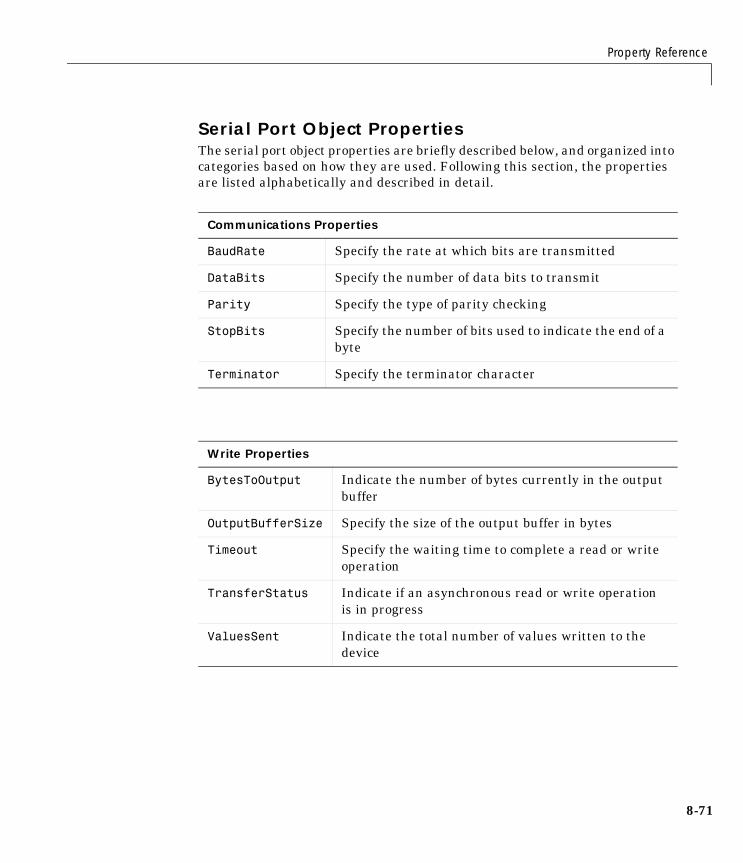
Property Reference
8-71
Serial Port Object PropertiesThe serial port object properties are briefly described below, and organized into categories based on how they are used. Following this section, the properties are listed alphabetically and described in detail.
Communications Properties
BaudRate Specify the rate at which bits are transmitted
DataBits Specify the number of data bits to transmit
Parity Specify the type of parity checking
StopBits Specify the number of bits used to indicate the end of a byte
Terminator Specify the terminator character
Write Properties
BytesToOutput Indicate the number of bytes currently in the output buffer
OutputBufferSize Specify the size of the output buffer in bytes
Timeout Specify the waiting time to complete a read or write operation
TransferStatus Indicate if an asynchronous read or write operation is in progress
ValuesSent Indicate the total number of values written to the device

8 Serial Port I/O
8-72
Read Properties
BytesAvailable Indicate the number of bytes available in the input buffer
InputBufferSize Specify the size of the input buffer in bytes
ReadAsyncMode Specify whether an asynchronous read operation is continuous or manual
Timeout Specify the waiting time to complete a read or write operation
TransferStatus Indicate if an asynchronous read or write operation is in progress
ValuesReceived Indicate the total number of values read from the device
Callback Properties
BreakInterruptFcn
Specify the M-file callback function to execute when a break-interrupt event occurs
BytesAvailableFcn
Specify the M-file callback function to execute when a specified number of bytes is available in the input buffer, or a terminator is read
BytesAvailableFcnCount
Specify the number of bytes that must be available in the input buffer to generate a bytes-available event
BytesAvailableFcnMode
Specify if the bytes-available event is generated after a specified number of bytes is available in the input buffer, or after a terminator is read
ErrorFcn Specify the M-file callback function to execute when an error event occurs
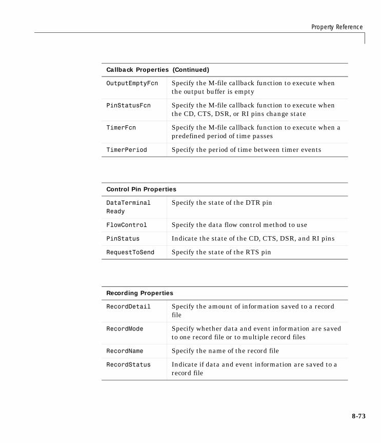
Property Reference
8-73
OutputEmptyFcn Specify the M-file callback function to execute when the output buffer is empty
PinStatusFcn Specify the M-file callback function to execute when the CD, CTS, DSR, or RI pins change state
TimerFcn Specify the M-file callback function to execute when a predefined period of time passes
TimerPeriod Specify the period of time between timer events
Control Pin Properties
DataTerminalReady
Specify the state of the DTR pin
FlowControl Specify the data flow control method to use
PinStatus Indicate the state of the CD, CTS, DSR, and RI pins
RequestToSend Specify the state of the RTS pin
Recording Properties
RecordDetail Specify the amount of information saved to a record file
RecordMode Specify whether data and event information are saved to one record file or to multiple record files
RecordName Specify the name of the record file
RecordStatus Indicate if data and event information are saved to a record file
Callback Properties (Continued)
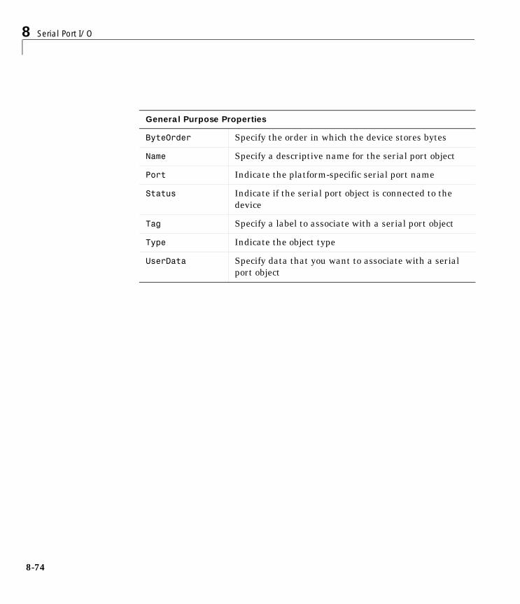
8 Serial Port I/O
8-74
General Purpose Properties
ByteOrder Specify the order in which the device stores bytes
Name Specify a descriptive name for the serial port object
Port Indicate the platform-specific serial port name
Status Indicate if the serial port object is connected to the device
Tag Specify a label to associate with a serial port object
Type Indicate the object type
UserData Specify data that you want to associate with a serial port object
I-1
Index
Symbols%val 3-5, 3-8
allocating memory 3-25DIGITAL Visual Fortran 3-8
AActiveX
automation client 7-4automation server 7-4, 7-16callback 7-8client support 7-6collections 7-10concepts 7-3control containment 7-4controller 7-16Count property 7-10event handler function 7-8events 7-3Execute method 7-16integration 7-3interface 7-3
custom 7-4standard 7-4
invoking event 7-8Item method 7-10launching server 7-21limitations of MATLAB support 7-13MATLAB as automation client 7-13methods 7-3object model 7-3ProgID 7-6properties 7-3server 7-16use in the MATLAB Engine 4-4
add-inMATLAB for Visual Studio 1-29
APIaccess methods 1-4memory management 1-37
argument checking 2-9argument passing, from Java methods
data conversion 5-56built-in data types 5-57conversions you can perform 5-57Java objects 5-57
argument passing, to Java methodsdata conversion 5-46
built-in arrays 5-48built-in data types 5-48Java object arrays 5-52Java object cell arrays 5-53Java objects 5-50objects of Object class 5-51string arrays 5-50string data types 5-49
effect of dimension on 5-53argument type, Java
effect on method dispatching 5-54array access methods 3-7
mat 6-3arrays
cell 1-8empty 1-9hybrid 2-40logical 1-9MATLAB 1-6multidimensional 1-8persistent 2-38serial port object 8-26sparse 2-29temporary 2-38, 3-37
arrays, Java
Index
I-2
accessing elements of 5-36assigning
the empty matrix 5-41values to 5-39with single subscripts 5-40
comparison with MATLAB arrays 5-30concatenation of 5-43creating a copy 5-45creating a reference 5-44creating in MATLAB 5-34creating with javaArray 5-34dimensionality of 5-30dimensions 5-33indexing 5-32
with colon operator 5-37with single subscripts 5-36, 5-38
linear arrays 5-41passed by reference 5-49representing in MATLAB 5-30sizing 5-32subscripted deletion 5-42using the end subscript 5-39
ASCII file mode 6-6ASCII flat file 6-4automation
client 7-13controller 7-16server 7-16
Bbcc53engmatopts.bat 1-18bcc53opts.bat 1-17bcc54engmatopts.bat 1-18bcc54opts.bat 1-17bcc55engmatopts.bat 1-18bcc55opts.bat 1-17
bccengmatopts.bat 1-18bccopts.bat 1-17binary data
reading from a device 8-41writing to a device 8-36
binary file mode 6-6BLAS and LAPACK functions 2-40
building MEX files for 2-44example of 2-46handling complex numbers 2-42passing arguments 2-41specifying the function name 2-41
BSTR 7-17buffer
input, serial port object 8-38output, serial port object 8-32
CC example
convec.c 2-21doubleelem.c 2-24findnz.c 2-26fulltosparse.c 2-29phonebook.c 2-17revord.c 2-11sincall.c 2-33timestwo.c 2-8timestwoalt.c 2-10xtimesy.c 2-14
C languagedata types 1-9debugging 2-47MEX-files 2-1
C language examplebasic 2-8calling MATLAB functions 2-33
Index
I-3
calling user-defined functions 2-33handling 8-, 16-, 32-bit data 2-23handling arrays 2-25handling complex data 2-21handling sparse arrays 2-29passing multiple values 2-13persistent array 2-39strings 2-11
callback 7-8serial port object 8-48
functions 8-52properties 8-49
caller workspace 2-37cat
using with Java arrays 5-43using with Java objects 5-12
cell 1-9using with Java objects 5-60
cell arrays 1-8, 2-16converting from Java object 5-60
char 1-9overloading toChar in Java 5-58
class
using in Java 5-17classes, Java 5-5
built-in 5-5defining 5-5identifying using which 5-25importing 5-8loading into workspace 5-7making available to MATLAB 5-6sources for 5-5third-party 5-5user-defined 5-5
classpath.txt
finding and editing 5-7using with Java archive files 5-6
using with Java classes 5-6using with Java packages 5-6
client (DDE) 7-23collections 7-10colon
using in Java array access 5-37using in Java array assignment 5-41
COM (component object model) 7-3object model 7-4
commands. See individual commands.Compaq Visual Fortran compiler
debugging 3-39compiler
changing on UNIX 1-12debugging
Compaq Visual Fortran 3-39Microsoft 2-48Watcom 2-49
preconfigured options file 1-17–1-19selecting on Windows 1-14supported 1-11
compilingengine application
UNIX 4-18–4-19Windows 4-19
MAT-file applicationUNIX 6-29Windows 6-30
complex datain Fortran 3-22
compopts.bat 1-23computational routine 2-3, 3-3concatenation
of Java arrays 5-43of Java objects 5-12
configuration 1-11problems 1-35

Index
I-4
UNIX 1-12Windows 1-14, 1-16
control pinsserial port object, using 8-56
convec.c 2-21convec.f 3-22conversation (DDE) 7-23conversion, data
in Java method arguments 5-46copying a Java array 5-45Count property 7-10cxxopts.sh 1-19
Ddata access
within Java objects 5-16data bits 8-13data format
serial port 8-11data storage 1-6data type 2-7
C language 1-9cell arrays 1-8checking 2-9complex double-precision nonsparse matrix
1-7empty arrays 1-9Fortran language 1-9logical arrays 1-9MAT-file 6-6MATLAB 1-9MATLAB string 1-7multidimensional arrays 1-8numeric matrix 1-7objects 1-8sparse arrays 2-29
sparse matrices 1-7structures 1-8
data, MATLAB 1-6exporting from 6-4–6-5importing to 6-3–6-4
dblmat.f 3-25dbmex 3-38DCE 8-5DCOM (distributed component object model) 7-22
using MATLAB as a server 7-22DDE (dynamic data exchange) 7-23
accessing MATLAB as server 7-25advisory links 7-32client 7-23conversation 7-23hot link 7-32item 7-24MATLAB
requesting data from 7-28sending commands to 7-27sending data to 7-29using as client 7-31
name hierarchy 7-26notifying when data changes 7-32server 7-23service name 7-24topic 7-24, 7-26–7-30
engine 7-27system 7-26
warm link 7-32Windows clipboard formats 7-24–7-25
ddeadv 7-31ddeexec 7-31ddeinit 7-31ddepoke 7-31ddereq 7-31ddeterm 7-31
Index
I-5
ddeunadv 7-31debugging C language MEX-files 2-47
UNIX 2-47Windows 2-48
debugging Fortran language MEX-filesUNIX 3-38Windows 3-39
DEC Alphadeclaring pointers 3-5
df50engmatopts.bat 1-19df50opts.bat 1-18df60engmatopts.bat 1-19df60opts.bat 1-18diary 6-4diary file 6-4DIGITAL Visual Fortran compiler
debugging 3-39directory
eng_mat 1-47mex 1-47mx 1-47refbook 1-46
directory organizationMAT-file application 6-8Microsoft Windows 1-44UNIX 1-42
directory pathconvention 1-2
displayserial port object 8-25
display functionoverloading toString in Java 5-26
distributed component object model. See DCOM.dll extension 1-4DLLs 1-11
locating 1-32documenting MEX-file 2-37, 3-36
double 1-9overloading toDouble in Java 5-58
doubleelem.c 2-24DTE 8-5dynamic data exchange. See DDE.dynamic memory allocation
in Fortran 3-25mxCalloc 2-11
dynamically linked subroutines 1-3
Eempty arrays 1-9empty matrix
conversion to Java NULL 5-54in Java array assignment 5-41
empty stringconversion to Java object 5-54
enduse with Java arrays 5-39
eng_mat directory 1-47, 4-6engClose 4-3, 4-4engdemo.c 4-6engEvalString 4-4engGetArray 4-3engGetMatrix 4-4engGetVisible 4-4engine
compiling 4-17linking 4-17UNIX 4-18windows 4-19
engine applicationWindows 4-19
engine examplecalling MATLAB
from C program 4-6
Index
I-6
from Fortran program 4-11engine functions 4-3–4-4engine library 4-2
communicating with MATLABUNIX 4-4Windows 4-4
engOpen 4-3, 4-4engOpenSingleUse 4-4engopts.sh 1-19engOutputBuffer 4-4engPutArray 4-3engPutMatrix 4-4engSetVisible 4-4engwindemo.c 4-6, 6-24event handler
function 7-8writing 7-8
eventsserial port object 8-48
storing information 8-50types 8-49
examples, Java programmingcommunicating through a serial port 5-68creating and using a phone book 5-73finding an internet protocol address 5-66reading a URL 5-63
exceptionfloating-point 4-17, 6-28
exceptions, Javahandling 5-28
explore example 1-9extension
MEX-file 1-3
F-f option 1-17
fengdemo.f 4-11fieldnames
using with Java objects 5-15file mode
ASCII 6-6binary 6-6
filesflat 6-4linking multiple 2-37, 3-36
findnz.c 2-26floating-point exceptions
Borland C++ Compiler on Windows 4-17, 6-28engine applications 4-17masking 4-17, 6-28MAT-file applications 6-28
fopen 6-4, 6-5Fortran
case in 3-6data types 1-9pointers
concept 3-5, 3-17declaring 3-5
Fortran examplesconvec.f 3-22dblmat.f 3-25fulltosparse.f 3-28matsq.f 3-17passstr.f 3-15revord.f 3-12sincall.f 3-32timestwo.f 3-10xtimesy.f 3-19
Fortran language examplescalling MATLAB functions 3-32handling complex data 3-22handling sparse matrices 3-28passing arrays of strings 3-14
Index
I-7
passing matrices 3-17passing multiple values 3-19passing scalar 2-7, 3-10passing strings 3-12
Fortran language MEX-files 3-3components 3-3
fread 6-4fulltosparse.c 2-29fulltosparse.f 3-28function handles
serial port object callback 8-52fwrite 6-5
G-g option 2-47gateway routine 2-3, 3-3, 3-6
accessing mxArray data 2-3gccopts.sh 1-19GetFullMatrix 7-17
Hhandshaking
serial port object 8-59help 2-37, 3-36help files 2-37, 3-36hybrid array
persistent 2-40temporary 2-40
hybrid arrays 2-40
IIDE
building MEX-files 1-20IEEE routines 1-4
import
using with Java classes 5-8include directory 6-9indexing Java arrays
using single colon subscripting 5-38using single subscripting 5-36
internet protocol addressJava example 5-66
ir 1-7, 2-29, 3-28isa
using with Java objects 5-18isjava
using with Java objects 5-18Item method 7-10
JJava
API class packages 5-3archive (JAR) files 5-6development kit 5-5Java Virtual Machine (JVM) 5-3packages 5-6
Java, MATLAB interface toarguments passed to Java methods 5-46arguments returned from Java methods 5-56arrays, working with 5-29benefits of 5-3classes, using 5-5examples 5-62methods, invoking 5-19objects, creating and using 5-10overview 5-3
javaArray function 5-34jc 1-7, 2-29, 3-28
Index
I-8
LLAPACK and BLAS functions 2-40
building MEX files for 2-44example of 2-46handling complex numbers 2-42passing arguments 2-41specifying the function name 2-41
lccengmatopts.bat 1-18lccopts.bat 1-17library path
setting on UNIX 4-18, 6-29linking DLLs to MEX-files 1-28linking multiple files 2-37, 3-36load 6-4, 6-6
using with Java objects 5-14loading
serial port objects 8-68locating DLLs 1-32logical arrays 1-9
Mmat.h 6-9matClose 6-7matDeleteArray 6-7matDeleteMatrix 6-8matdemo1.f 6-21matdemo2.f 6-24MAT-file
C languagereading 6-16
compiling 6-28data types 6-6examples 6-9Fortran language
creating 6-21reading 6-24
linking 6-28overview 6-2subroutines 6-6UNIX libraries 6-9using 6-3Windows libraries 6-9
MAT-file applicationUNIX 6-29Windows 6-30
MAT-file examplecreating
C language 6-11Fortran language 6-21
readingC language 6-16Fortran language 6-24
MAT-functions 6-7–6-8matGetArray 6-7matGetArrayHeader 6-7matGetDir 6-7, 6-8matGetFp 6-7matGetMatrix 6-8matGetNextArray 6-7matGetNextArrayHeader 6-7matGetNextMatrix 6-8matGetString 6-8MATLAB
ActiveX interface 7-10arrays 1-6as DCOM server client 7-12data 1-6data file format 6-3data storage 1-6data type 1-9engine 4-2exporting data 6-3–6-5importing data 6-3–6-4
Index
I-9
MAT-file 6-6reading arrays from 6-6saving arrays to 6-6
moving data between platforms 6-5–6-6stand-alone applications 6-2, 6-3string 1-7using as a computation engine 4-2variables 1-6
MATLAB add-in for Visual Studioconfiguring on Windows 95 and 98 1-30configuring on Windows ME 1-30
MATLAB Automation Serversupported methods 7-17
MATLAB for Visual Studio add-in 1-29matOpen 6-7matopts.sh 1-19matPutArray 6-7matPutArrayAsGlobal 6-7matPutMatrix 6-8matPutString 6-8matrix
complex double-precision nonsparse 1-7numeric 1-7sparse 1-7, 3-28
matrix.h 6-9matsq.f 3-17memory
allocation 2-11leak 1-40, 2-38temporary 3-37
memory management 1-37, 2-38, 3-37API 1-37compatibility 1-37routines 1-4special considerations 2-38
methods
using with Java methods 5-24
methods, Javacalling syntax 5-19converting input arguments 5-46displaying 5-24displaying information about 5-22finding the defining class 5-25overloading 5-54passing data to 5-46static 5-21undefined 5-27
methodsview 5-22output fields 5-24
mex
<ENV_VAR>#<val> 1-22-g 2-47, 3-38
mex build script 1-20, 2-9default options file, UNIX 1-22default options file, Windows 1-23switches 1-21
<name>#<def> 1-22<name>=<def> 1-22@<rsp_file> 1-21-argcheck 1-21-c 1-21-D<name>[#<def>] 1-21-f <file> 1-21-fortran 3-36-g 1-21-h[elp] 1-21-I<pathname> 1-21-inline 1-21-l<file> 1-21-L<pathname> 1-21-O 1-22-outdir <name> 1-22-output <name> 1-22-setup 1-14, 1-22
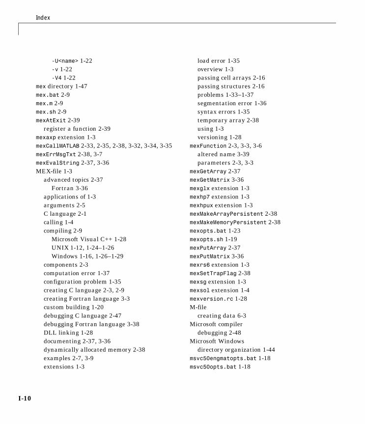
Index
I-10
-U<name> 1-22-v 1-22-V4 1-22
mex directory 1-47mex.bat 2-9mex.m 2-9mex.sh 2-9mexAtExit 2-39
register a function 2-39mexaxp extension 1-3mexCallMATLAB 2-33, 2-35, 2-38, 3-32, 3-34, 3-35mexErrMsgTxt 2-38, 3-7mexEvalString 2-37, 3-36MEX-file 1-3
advanced topics 2-37Fortran 3-36
applications of 1-3arguments 2-5C language 2-1calling 1-4compiling 2-9
Microsoft Visual C++ 1-28UNIX 1-12, 1-24–1-26Windows 1-16, 1-26–1-29
components 2-3computation error 1-37configuration problem 1-35creating C language 2-3, 2-9creating Fortran language 3-3custom building 1-20debugging C language 2-47debugging Fortran language 3-38DLL linking 1-28documenting 2-37, 3-36dynamically allocated memory 2-38examples 2-7, 3-9extensions 1-3
load error 1-35overview 1-3passing cell arrays 2-16passing structures 2-16problems 1-33–1-37segmentation error 1-36syntax errors 1-35temporary array 2-38using 1-3versioning 1-28
mexFunction 2-3, 3-3, 3-6altered name 3-39parameters 2-3, 3-3
mexGetArray 2-37mexGetMatrix 3-36mexglx extension 1-3mexhp7 extension 1-3mexhpux extension 1-3mexMakeArrayPersistent 2-38mexMakeMemoryPersistent 2-38mexopts.bat 1-23mexopts.sh 1-19mexPutArray 2-37mexPutMatrix 3-36mexrs6 extension 1-3mexSetTrapFlag 2-38mexsg extension 1-3mexsol extension 1-4mexversion.rc 1-28M-file
creating data 6-3Microsoft compiler
debugging 2-48Microsoft Windows
directory organization 1-44msvc50engmatopts.bat 1-18msvc50opts.bat 1-18
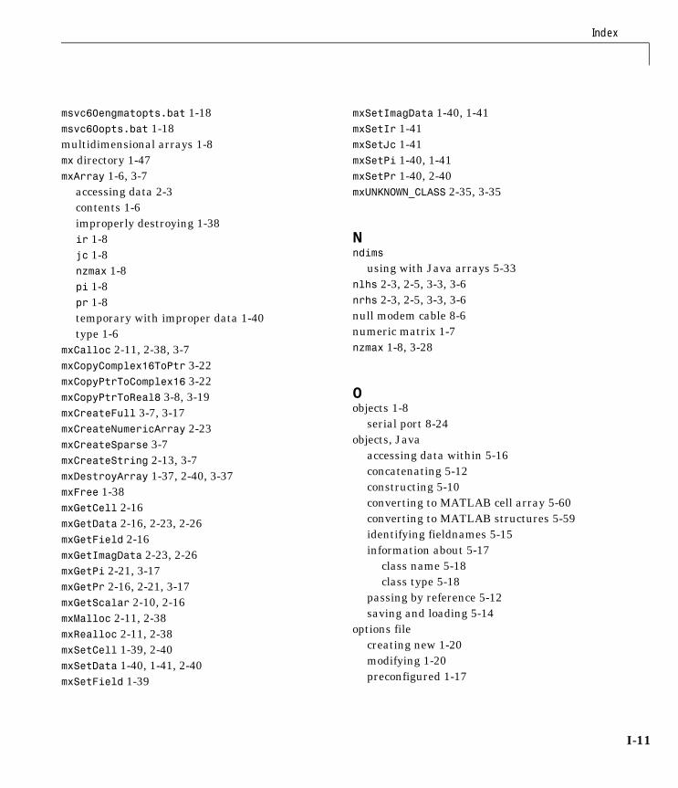
Index
I-11
msvc60engmatopts.bat 1-18msvc60opts.bat 1-18multidimensional arrays 1-8mx directory 1-47mxArray 1-6, 3-7
accessing data 2-3contents 1-6improperly destroying 1-38ir 1-8jc 1-8nzmax 1-8pi 1-8pr 1-8temporary with improper data 1-40type 1-6
mxCalloc 2-11, 2-38, 3-7mxCopyComplex16ToPtr 3-22mxCopyPtrToComplex16 3-22mxCopyPtrToReal8 3-8, 3-19mxCreateFull 3-7, 3-17mxCreateNumericArray 2-23mxCreateSparse 3-7mxCreateString 2-13, 3-7mxDestroyArray 1-37, 2-40, 3-37mxFree 1-38mxGetCell 2-16mxGetData 2-16, 2-23, 2-26mxGetField 2-16mxGetImagData 2-23, 2-26mxGetPi 2-21, 3-17mxGetPr 2-16, 2-21, 3-17mxGetScalar 2-10, 2-16mxMalloc 2-11, 2-38mxRealloc 2-11, 2-38mxSetCell 1-39, 2-40mxSetData 1-40, 1-41, 2-40mxSetField 1-39
mxSetImagData 1-40, 1-41mxSetIr 1-41mxSetJc 1-41mxSetPi 1-40, 1-41mxSetPr 1-40, 2-40mxUNKNOWN_CLASS 2-35, 3-35
Nndims
using with Java arrays 5-33nlhs 2-3, 2-5, 3-3, 3-6nrhs 2-3, 2-5, 3-3, 3-6null modem cable 8-6numeric matrix 1-7nzmax 1-8, 3-28
Oobjects 1-8
serial port 8-24objects, Java
accessing data within 5-16concatenating 5-12constructing 5-10converting to MATLAB cell array 5-60converting to MATLAB structures 5-59identifying fieldnames 5-15information about 5-17
class name 5-18class type 5-18
passing by reference 5-12saving and loading 5-14
options filecreating new 1-20modifying 1-20preconfigured 1-17
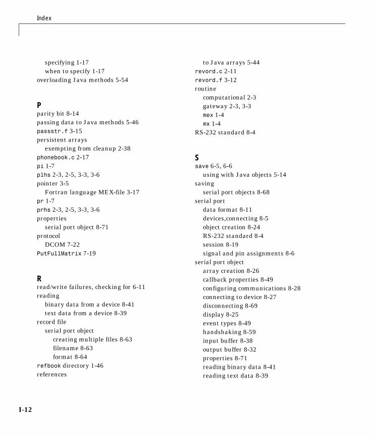
Index
I-12
specifying 1-17when to specify 1-17
overloading Java methods 5-54
Pparity bit 8-14passing data to Java methods 5-46passstr.f 3-15persistent arrays
exempting from cleanup 2-38phonebook.c 2-17pi 1-7plhs 2-3, 2-5, 3-3, 3-6pointer 3-5
Fortran language MEX-file 3-17pr 1-7prhs 2-3, 2-5, 3-3, 3-6properties
serial port object 8-71protocol
DCOM 7-22PutFullMatrix 7-19
Rread/write failures, checking for 6-11reading
binary data from a device 8-41text data from a device 8-39
record fileserial port object
creating multiple files 8-63filename 8-63format 8-64
refbook directory 1-46references
to Java arrays 5-44revord.c 2-11revord.f 3-12routine
computational 2-3gateway 2-3, 3-3mex 1-4mx 1-4
RS-232 standard 8-4
Ssave 6-5, 6-6
using with Java objects 5-14saving
serial port objects 8-68serial port
data format 8-11devices,connecting 8-5object creation 8-24RS-232 standard 8-4session 8-19signal and pin assignments 8-6
serial port objectarray creation 8-26callback properties 8-49configuring communications 8-28connecting to device 8-27disconnecting 8-69display 8-25event types 8-49handshaking 8-59input buffer 8-38output buffer 8-32properties 8-71reading binary data 8-41reading text data 8-39
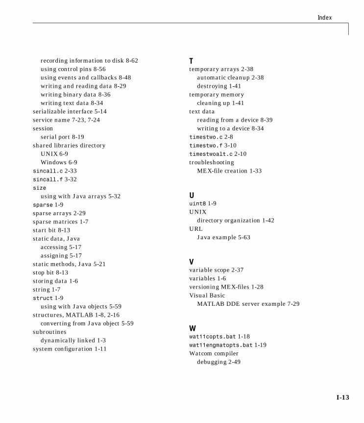
Index
I-13
recording information to disk 8-62using control pins 8-56using events and callbacks 8-48writing and reading data 8-29writing binary data 8-36writing text data 8-34
serializable interface 5-14service name 7-23, 7-24session
serial port 8-19shared libraries directory
UNIX 6-9Windows 6-9
sincall.c 2-33sincall.f 3-32size
using with Java arrays 5-32sparse 1-9sparse arrays 2-29sparse matrices 1-7start bit 8-13static data, Java
accessing 5-17assigning 5-17
static methods, Java 5-21stop bit 8-13storing data 1-6string 1-7struct 1-9
using with Java objects 5-59structures, MATLAB 1-8, 2-16
converting from Java object 5-59subroutines
dynamically linked 1-3system configuration 1-11
Ttemporary arrays 2-38
automatic cleanup 2-38destroying 1-41
temporary memorycleaning up 1-41
text datareading from a device 8-39writing to a device 8-34
timestwo.c 2-8timestwo.f 3-10timestwoalt.c 2-10troubleshooting
MEX-file creation 1-33
Uuint8 1-9UNIX
directory organization 1-42URL
Java example 5-63
Vvariable scope 2-37variables 1-6versioning MEX-files 1-28Visual Basic
MATLAB DDE server example 7-29
Wwat11copts.bat 1-18wat11engmatopts.bat 1-19Watcom compiler
debugging 2-49
Index
I-14
watcopts.bat 1-18watengmatopts.bat 1-19which
using with Java methods 5-25Windows
ActiveX 7-16automation 7-16directory organization 1-44mex -setup 1-14selecting compiler 1-14
Windows clipboard formatMetafilepict 7-25text 7-24XLTable 7-25
workspacecaller 2-37, 3-36MEX-file function 2-37, 3-36
write/read failures, checking for 6-11writing
binary data to a device 8-36text data to a device 8-34
writing event handlers 7-8
Xxtimesy.c 2-14xtimesy.f 3-19
Yyprime.c 1-12, 1-16yprimef.F 1-12yprimef.f 1-16yprimefg.F 1-12yprimefg.f 1-16