Embed Size (px)
Citation preview

Honours Year Project Report
Computational analysis of genotypes
produced by fluoMEP
By
Rashmi Sukumaran
Department of Computer Science
School of Computing
National University of Singapore
2007/2008

Honours Year Project Report
Computational analysis of genotypes
produced by fluoMEP
By
Rashmi Sukumaran
Department of Computer Science
School of Computing
National University of Singapore
2007/2008
Project No: H114140
Project Advisor: Prof. Wong Lim Soon
Dr. Laszlo Orban, TLL (Adjunct Assoc. Prof. to DBS/NUS)
Deliverables:
Report: 1 Volume
Program: 1 Diskette

ii
Abstract FluoMEP, a mass genotyping method combining the advantages of RAPD and AFLP, was developed recently in the host lab at TLL. It allows for automatic detection of labeled amplified fragments as peaks by a scanner. However analysis of the enormous amount of data generated is currently done by manually scoring the peaks as present or absent, which is tedious. Furthermore manual analysis is prone to human error due to differences in peak intensities and positions. Thus there is a need to automate the data analysis process which is also able to screen for differences by comparison of peak heights and shifts. Existing softwares for analyzing AFLP data are not suited for fluoMEP experimental design. In this project, I created a new software called FluoMEP Marker Finder (FMF) for analyzing fluoMEP data. For assessment, seven Nile tilapia fluoMEP datasets, where sex markers were identified previously by manual analysis, were re-analyzed using the newly developed software. FMF finds 13% more markers than manual analysis, shortens time for analysis by 6000 times and improves sensitivity and precision by at least 3 folds. FMF is the first automation developed for analysis of fluoMEP data and can be used for future datasets of any kind. Subject Descriptors: I.5 Pattern Recognition J.3 Life and Medical Sciences Keywords: FluoMEP, Genotyping, Analysis tool Implementation Software: Java and Windows XP

iii
Acknowledgement I would like to express my deepest gratitude to both my supervisors – Dr. Laszlo Orban,
(Temasek Life Sciences Laboratory; Adjunct Assoc. Prof. to DBS/NUS) and Prof. Wong
Lim Soon (SOC/NUS) – for their valuable guidance in this project. They have supported
and helped me in every way, for the successful completion of this project.
I am also grateful to Mr. Liew Woei Chang (TLL), for being a wonderful mentor, who
provided constructive inputs and numerous suggestions, which helped improve my
understanding of the whole project and thus, improve the quality of implementation.
I am also thankful to Mr. Lin Qifeng (NUS/TLL), for his constant support throughout the
project. He provided me with technical help in understanding the fluoMEP procedure and
the data produced, which was crucial for the development phase of the implementation.
I am also grateful to Ms. Jolly M Saju (TLL), for providing me with ‘real-life’ datasets to
evaluate my software. I also thank her students Ms. Aziemah and Ms. Jeanette, for
producing the datasets.

iv
Table of Contents
Title Page i
Abstract ii
Acknowledgement iii
1 Introduction 1
1.1 Background 1
1.1.1 Randomly Amplified Polymorphic DNA 2
1.1.2 Amplified Fragment Length Polymorphism 3
1.2 FluoMEP 4
1.2.1 Current applications of fluoMEP 6
1.2.2 Current problem 7
1.3 Aim of my Honours project 8
2 Materials and Methods 9
2.1 Experimental Data used 9
2.2 FluoMEP screening 10
2.3 Software development 11
2.4 Software Evaluation 11
3 Implementation 11
3.1 Overview of the FMF architecture 11
3.2 Input Data Format 12
3.3 Application Logic of the software 13
3.3.1 Issues during analysis 14
3.3.2 Application Logic of FMF 15
3.4 Output Data Format 20
3.5 Graphical User Interface (GUI) 21
4 Results and Discussion 23
4.1 Evaluation of FMF 23
4.1.1 Number of potential male markers obtained 24
4.1.2 Agreements and disagreements on the potential markers found 25

v
4.2 Performance of FMF 29
4.3 Benefits of FMF 31
4.3.1 Immediate benefits 31
4.3.2 Long-term benefits 31
4.4 Drawbacks of FMF 31
5 Related Work 32
6 Future Work 35
7 Conclusion 35
References iv
Appendix A vi

1
1 Introduction Genotyping is the process of determining the whole or partial genotype (i.e. DNA
sequence) of an individual using a biological assay.
One main application of genotyping is to study the differences between the DNA
sequence of individuals of a species, accounting for one or more observable traits, like,
sex of the individual or a disease. These differences closely linked to different variations
of a particular trait are called polymorphic molecular markers or DNA markers. In
bisexual species, markers seen in the genotype of only one sex are called sex-specific
markers.
1.1 Background
Most current genotyping methods involve Polymerase Chain Reaction (PCR;
Mullis and Faloona, 1987; Saiki, et al. 1985), a molecular biology technique used to
amplify a DNA template. In traditional PCR, primers (short oligonucleotides) are
designed to be complementary to the start / end of template to be amplified. During the
reaction the primers bind to the DNA template and DNA polymerase proceeds to
duplicate the portion of the template enclosed by the primers, as shown in Figure 1. Thus,
traditional PCR requires the preliminary information about the DNA template to design
the primers.
However, this preliminary sequence information is not always available during
genotyping. Over the past two decades, researchers have developed various methods to
derive information from unknown genomes. Most of these methods are based on PCR.
PCR Product
Primer
DNA Template
Figure 1: Schematic representation of traditional PCR. The primers (green arrows) bind to the part of the template complementary to it (green) and DNA polymerase duplicates the remaining part of the template (black). The PCR product obtained is exactly same as the template used and thus can be used as a template in the next cycle of PCR.

2
Two popular PCR-based genotyping methods are Randomly Amplified Polymorphic
DNA (RAPD) and Amplified Fragment Length Polymorphism (AFLP).
1.1.1 Randomly Amplified Polymorphic DNA
RAPD is a specialized PCR reaction where the template to be amplified is
unknown. RAPD uses short (8-12mer) oligonucleotide primer, created arbitrarily, to
amplify fragments from a long template of genomic DNA (Williams, Kubelik, Livak,
Rafalski and Tingey, 1990; Welsh and McClelland, 1990). The primers used may bind to
the DNA template at multiple locations, depending on positions on the template
complementary to the primers. When the amplified products are separated on a gel, a set
of bands is seen, as shown in Figure 2. Each fragment of template amplified would be
seen as a band. If, for example, polymorphism occurs in the region of the template
previously complementary to the primer, no band would be seen. Thus, RAPD products
from two different DNA samples can be compared to find the markers.
The main advantage of RAPD is its user-friendliness. It is easy to setup and
relatively simple to use. However, certain shortcomings like (i) non-reproducibility
across different labs due to sensitivity to reagents (de Vicente and Fulton, 2003); (ii)
ambiguity in the interpretation of results as absence of a band due to lack of target
sequence cannot be differentiated from that due to other reasons like poor quality DNA
RAPD Products
RAPD Primer
Genomic DNA
Figure 2: Schematic representation of RAPD. The several copies of the arbitrary primer (green arrows) bind to the different parts of the template complementary to it (green) and DNA polymerase proceeds to amplify the bound region of the template if possible. The products obtained are amplified fragments of the template used. Each amplified fragment would be seen as a single band on the gel, during electrophoresis. Thus, a set of bands formed from every genomic DNA template amplified by RAPD as seen in the gel picture (Williams, et al, 1990).
3
(de Vicente, et al. 2003); and (iii) incompatibility to high-throughput methods due to the
gel electrophoresis separation method (Chang, et al. 2007) limit the use of RAPD. Thus,
the more robust AFLP has replaced RAPD in many applications.
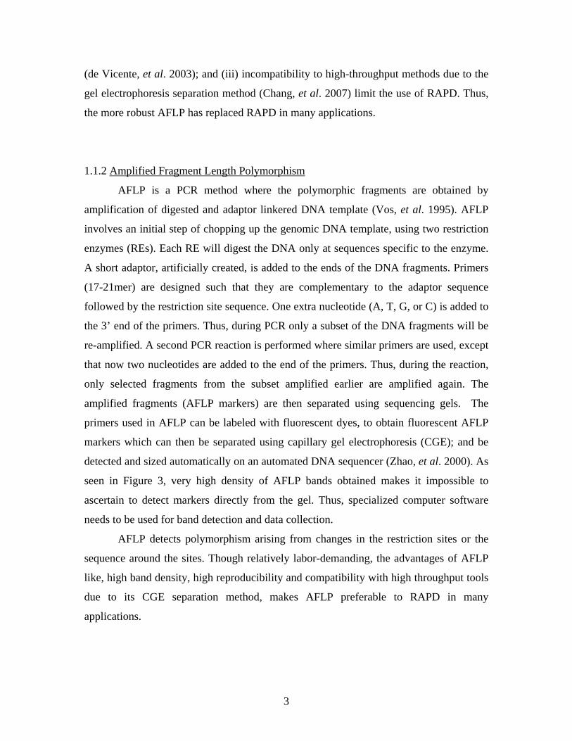
1.1.2 Amplified Fragment Length Polymorphism
AFLP is a PCR method where the polymorphic fragments are obtained by
amplification of digested and adaptor linkered DNA template (Vos, et al. 1995). AFLP
involves an initial step of chopping up the genomic DNA template, using two restriction
enzymes (REs). Each RE will digest the DNA only at sequences specific to the enzyme.
A short adaptor, artificially created, is added to the ends of the DNA fragments. Primers
(17-21mer) are designed such that they are complementary to the adaptor sequence
followed by the restriction site sequence. One extra nucleotide (A, T, G, or C) is added to
the 3’ end of the primers. Thus, during PCR only a subset of the DNA fragments will be
re-amplified. A second PCR reaction is performed where similar primers are used, except
that now two nucleotides are added to the end of the primers. Thus, during the reaction,
only selected fragments from the subset amplified earlier are amplified again. The
amplified fragments (AFLP markers) are then separated using sequencing gels. The
primers used in AFLP can be labeled with fluorescent dyes, to obtain fluorescent AFLP
markers which can then be separated using capillary gel electrophoresis (CGE); and be
detected and sized automatically on an automated DNA sequencer (Zhao, et al. 2000). As
seen in Figure 3, very high density of AFLP bands obtained makes it impossible to
ascertain to detect markers directly from the gel. Thus, specialized computer software
needs to be used for band detection and data collection.
AFLP detects polymorphism arising from changes in the restriction sites or the
sequence around the sites. Though relatively labor-demanding, the advantages of AFLP
like, high band density, high reproducibility and compatibility with high throughput tools
due to its CGE separation method, makes AFLP preferable to RAPD in many
applications.

4
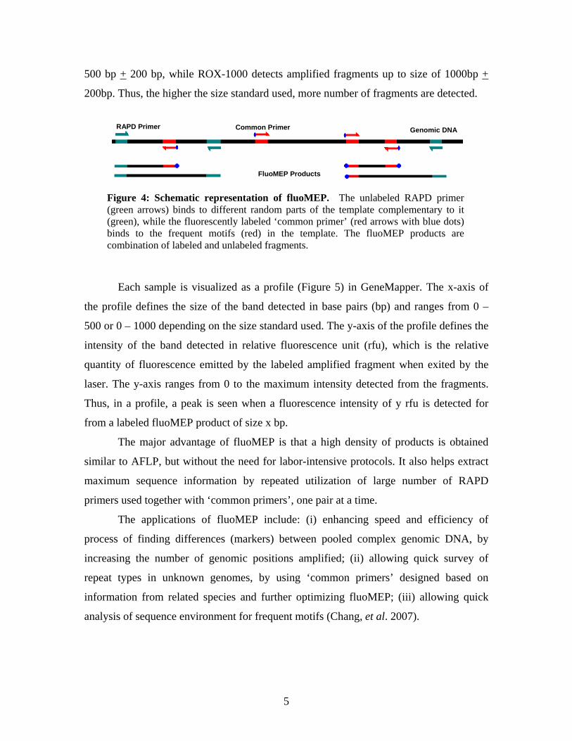
1.2 FluoMEP
A new genotyping method, combining the advantages of RAPD and AFLP, was
recently developed in the host lab Reproductive Genomics Group (RGG) at Temasek Life
Sciences Laboratory (TLL). Fluorescent Motif Enhanced Polymorphism (fluoMEP) is
based on RAPD assay, but draws in the advantage of large-scale use of commercial
RAPD primers and the power of automated CGE devices used in AFLP, with the addition
of fluorescently labeled primers (Chang, et al. 2007). FluoMEP is a PCR reaction which
uses a combination of two-types of primers – unlabeled RAPD primers (~10 nucleotides)
and fluorescently labeled ‘common primers’ – to amplify genomic DNA template. A
schematic representation of fluoMEP is shown in Figure 4. ‘Common primers’ are so
named because they target the repeats and frequently occurring motifs in the genome.
Thus, by screening the template with one ‘common primer’ and a series of RAPD
primers, the template can be analyzed effectively (Chang, et al. 2007).
FluoMEP has two types of products – labeled and unlabeled. The labeled
fluoMEP products are separated by CGE run on an automatic sequencer. Similar to
AFLP, a high density of bands is obtained for fluoMEP as well. Thus, band detection,
data collection and visualization are done with the help of specialized software
GeneMapper. A size standard is a size reference used by GeneMapper, similar to the size
marker used in gel electrophoresis analysis of DNA. Different size standards are used to
detect fragments. The size standard also restricts the maximum size of the amplified
fragment detected. For example, ROX-500 detects amplified fragments up to the size of
Figure 3: AFLP pattern separated by an automatic sequencer (de Vicente, et al. 2003). The samples are labeled with one of three fluorescent dyes – yellow, blue or green. A control sample labeled in red is also seen. Due to the high density of the bands, it is impossible to ascertain the presence or absence of AFLP markers directly from the gel. Thus, band detection and data collection needs to be done with the help of specialized software.
5
500 bp + 200 bp, while ROX-1000 detects amplified fragments up to size of 1000bp +
200bp. Thus, the higher the size standard used, more number of fragments are detected.
Each sample is visualized as a profile (Figure 5) in GeneMapper. The x-axis of
the profile defines the size of the band detected in base pairs (bp) and ranges from 0 –
500 or 0 – 1000 depending on the size standard used. The y-axis of the profile defines the
intensity of the band detected in relative fluorescence unit (rfu), which is the relative
quantity of fluorescence emitted by the labeled amplified fragment when exited by the
laser. The y-axis ranges from 0 to the maximum intensity detected from the fragments.
Thus, in a profile, a peak is seen when a fluorescence intensity of y rfu is detected for
from a labeled fluoMEP product of size x bp.
The major advantage of fluoMEP is that a high density of products is obtained
similar to AFLP, but without the need for labor-intensive protocols. It also helps extract
maximum sequence information by repeated utilization of large number of RAPD
primers used together with ‘common primers’, one pair at a time.
The applications of fluoMEP include: (i) enhancing speed and efficiency of
process of finding differences (markers) between pooled complex genomic DNA, by
increasing the number of genomic positions amplified; (ii) allowing quick survey of
repeat types in unknown genomes, by using ‘common primers’ designed based on
information from related species and further optimizing fluoMEP; (iii) allowing quick
analysis of sequence environment for frequent motifs (Chang, et al. 2007).
FluoMEP Products
Genomic DNA RAPD Primer Common Primer
Figure 4: Schematic representation of fluoMEP. The unlabeled RAPD primer (green arrows) binds to different random parts of the template complementary to it (green), while the fluorescently labeled ‘common primer’ (red arrows with blue dots) binds to the frequent motifs (red) in the template. The fluoMEP products are combination of labeled and unlabeled fragments.

6
1.2.1 Current applications of fluoMEP
FluoMEP is being currently used for the isolation of sex-specific markers from
the genome of various fish species, including Nile tilapia. The latter project is
collaboration between GenoMar and TLL. GenoMar is among world leaders in life
science based breeding of marine and aquatic species. This commercial project aims to
improve the aquaculture production of GenoMar’s farm fish Nile tilapia (Oreochromis
niloticus).
Nile tilapia has differential growth rate and maturation time between the two
sexes – males tend to grow faster and produce more meat than the females. Thus, for
commercial purposes, monosex populations of males must be generated. Currently, all
populations are treated with male steroid hormone to achieve hormonal sex reversal of
females into males. Alternative, hormone-less or hormone-free methods are required and
(B)
1 2 3 4 5
3
5
4
2 1
(A)
Figure 5: Visualization of fluoMEP profiles in GeneMapper. (A) shows profile of a single sample amplified with one combination of primers, analyzed and visualized in GeneMapper. Each vertical line is a peak representing one labeled fluoMEP product. (B) shows a schematic representation of how the peaks seen in a fluoMEP profile are analogous to bands seen on a gel. The five bands seen in the schematic gel picture are in increasing order of size from the bottom and have varying intensities. This is reflected in the fluoMEP profile. The peaks are arranged in their increasing order of size from left to right. The height of the peaks corresponds to the intensity of the bands seen in the gel. Though bands one, three and five have the same intensity in the gel, band five is slightly thicker than the rest and thus, has a larger area under the curve in the profile.

7
they would benefit from the early identification of the sexes by using molecular sexing
methods.
However, finding sex-specific markers in Nile tilapia, whose genome has not yet
been sequenced, has to be done with the help of a genotyping method, like fluoMEP. Sex
chromosomes in Nile tilapia are not divergent enough to be recognized by direct
molecular methods. Through indirect methods, it has been suggested that, like humans,
Nile tilapia has an XX/XY-type sex determination system – XX females and XY males
(Mair, Scott, Penman, Beardmore, and Skibinski, 1991; Carrasco, Penman, and Bromage,
1999). Theoretically, sex-specific markers found in males would be absent in females.
Nile Tilapia project aims to create an all-male population with the help of
fluoMEP male markers (Y-specific markers). This is done in four stages: (i) determine
the Y-specific markers in adult Nile Tilapia using large-scale fluoMEP screening; (ii)
hormonally sex-reverse wild type male (XY) and identify the sex-reversed neo-females
(with XY genotype) by using the markers found; (iii) cross these neo-females (XY) with
wild type male (XY) and identify the YY males from the offsprings by testing their
babies with Y-specific molecular sex markers and (iv) cross these YY males with wild
type females (XX) to create an all-male population.
1.2.2 Current problem
First stage of the sexing process is currently on-going at the RGG lab. A list of
male-specific markers in Nile Tilapia is being determined with a series of fluoMEP
screening. Fin-clip samples from adult males are pooled together, usually, into one to two
groups. Samples from adult females are also pooled the same way. The male and female
pools are genotyped together, using a series of combinations of fluoMEP primers
(common primer + RAPD primer). GeneMapper profiles are obtained for each pool and
manually compared by eye, to find differences in the pattern of peaks between males and
females in each primer combination and thus, to find robust male-specific markers. For
pool screening, a male marker is considered robust if a significant peak is present in all
male pools and absent in all female pools, in that particular primer combination or if there
is a female peak, the male peak must be significantly larger than the female peak present.

8
Once a male marker is spotted, the individual samples (male and female) that
formed the pool are screened individually using the same fluoMEP primer combination.
Again, profiles are obtained and manually compared by eye, to verify if the male marker
spotted earlier is robust. For individual screening, a male marker is considered robust if a
significant peak is present in >80% of the male samples and absent in <80% of the
female samples.
Usually, one fluoMEP run is done in a 96-well plate. Depending on the number of
male and female in one primer combination, there are ‘n’ numbers of visual comparison
of profiles to be done. For example, if there are two male pools and one female pool
being amplified, there would be 32 (96 / 3) primer combinations being run in one-plate
and thus, 32 visual comparisons to be done manually. This can be quite time-consuming
and tedious. Also, it is prone to manual errors. Thus, the need for automation of the
process of comparison arises.
Existing software capable of similar analysis for AFLP data are not suitable to
analyze fluoMEP profiles, as they do not meet one or more requirements needed. Most of
the softwares convert profile data into binary data – i.e. peaks present or absent. If peaks
are present in both male and female, and the male peak is significantly larger than the
female peak, it could be a potential marker. However, in such a case, during the
conversion, both male and female would indicate peak present in binary and thus,
information loss occurs. Also, certain softwares are compatible only with Linux. Most
biologists being more familiar with Windows OS prefer windows compatible softwares.
1.3 Aim of my Honours project
Thus, in this Honours project, I aim to develop software capable of
computationally analyzing the genotype profiles produced by fluoMEP from two
different class of samples (e.g. male vs female, diseased vs normal) to detect markers
present in one class. The software must be able to satisfy the following conditions:
1. Able to report the size and intensity of robust markers
− For pooled samples, significant peak present in one class of samples and absent
in other class of samples in one primer combination

9
− For pooled samples, peak present in one class of samples significantly larger (~
3 times) than peaks present in other class
− For individual samples, significant peak present in a percentage of one class and
absent in a percentage of the other class
2. Provide a goodness measure for the markers reported
3. Output the report in user-friendly and easy to understand format
4. Provide a user-friendly interface.
2 Materials and Methods Experimental data used to evaluate the software is described in section 2.1. The
materials and methods used to generate the experimental data are briefly described in
section 2.2.
2.1 Experimental Data used
The fluoMEP datasets used to test the software were “real life” datasets from the
Nile tilapia project. All the datasets used in this project were kind contributions of Ms
Jolly M Saju (ARO, RGG) and her students.
A total of 7 datasets were analyzed. Five of the seven datasets contained data
from male and female pooled samples, while the remaining two contained data from
individual male and female samples.
Dataset 1 contained data of a total of 96 pooled samples. Each primer
combination in the dataset consisted of one male pool sample and one female pool
sample. Thus, dataset 1 contained 48 primer combinations to be analyzed.
Dataset 2 to dataset 5, each contained data of a total of 96 samples. Each primer
combination in all the four datasets consisted of two male pool samples and one female
pool sample. Thus, datasets 2-5 contained 32 primer combinations each, to be analyzed.
Dataset 6 and dataset 7 contained data of a total of 81 individual samples. Each
primer combination in the dataset consisted of seventeen male samples and ten female
pool samples. Thus, dataset 6 and 7 contained 3 primer combinations each, to be
analyzed.

10
Thus, a total of 642 samples in 182 primer combinations were analyzed for
evaluation.
2.2 FluoMEP screening
The source of DNA samples in the datasets used for fluoMEP screening for male-
specific markers was fin clips from adult male and female Nile tilapia (Oreochromis
niloticus), provided by GenoMar fish farm (Sembawang field station)
‘Common primers’ were designed using sequences from motifs that frequently
occur in the genome, like conserved splices sites, GATA/ GACA repeats and vertebrate
short interspersed nuclear elements (V-SINE) sequences (Chang, et al. 2007). The
primers (9 – 12 nucleotides) were designed using Primer Premier 5 software (Premier
Biosoft International, Palo Alto, CA, USA). The primers were synthesized and labeled
with either Fam or Hex fluorescent dyes by 1stBase Pte Ltd(Singapore).
RAPD primers (10 nucleotides) used were commercial primers from Operon
Biotechnologies (Cologne, Germany). The RAPD primers used in the datasets come in
batches of 20.
The fluoMEP assay was performed as described in Chang, et al. 2007. Dataset 1
was from 10 males and 10 females. The 10 males were pooled into one pool and 10
females were pooled into one pool. Each of the dataset 2-5 was from 17 males and 10
females. Out of the 17 males, nine were pooled into one pool and the remaining to
another pool. The 10 females were pooled together as one pool. Dataset 6 and 7 was from
27 individuals – 17 individual males and 10 individual females.
The labeled fluoMEP products were separated by CGE on 3730xl DNA Analyzer
(ABI, Foster City, CA, USA) sequencing machine using 50 cm long 96-well capillaries
filled with Pop-7 DNA analyzer polymer (ABI) gel matrix. Prior separation, the samples
were denatured (separation of double-stranded DNA) by addition of Hi-Di Formamide
(ABI) at 95°C. Peaks were detected by the GeneMapper v3.5 software (ABI). The size
standards for size reference for GeneMapper were labeled with 6-carboxy-X-rhodamine
(ROX). Dataset 1 was sized using ROX-500, while all other datasets were sized using
ROX-1000. The sizing table for each dataset was exported from GeneMapper as comma
separated values (csv) file, to be used as input for the software.

11
2.3 Software development
The software was developed in Java programming language, using NetBeans
Integrated Development Environment (IDE) v5.5 platform (Sun Microsystems, Santa
Clara, CA, USA).
2.4 Software Evaluation
The datasets were analyzed with the default settings: Male threshold = 300 rfu;
Female threshold = 0 rfu; Percentage of males required to show expression = 100
(pooled), 80 (individual); Percentage of females required not to show expression = 100
(pooled), 80 (individual); No. of folds = 3.
3 Implementation A new software called FluoMEP Marker Finder (FMF) was developed in this
project to analyze fluoMEP genotypes of two class of samples and to find markers
present in one of them. The details of the implementation are described in the following
sections.
3.1 Overview of the FMF architecture
The software FMF uses two-tier architecture: user-interface tier and the
application logic tier (Figure 6). The interface-tier offers the user a simple and convenient
way to communicate with the system. The application logic tier performs the
manipulation of the information. Thus, this architecture helps hide the technical details
and internal workings of the system from the user.
The input file and input parameters for analysis is set by the user using the
graphical user interface (GUI). The analysis is carried out by FMF and an output file
containing the results is created in the same folder or directory as the input file.

12
3.2 Input Data Format
FMF supports only comma separated values (csv) file formats. CSV files are text
documents with data values separated by commas. They are compatible with Microsoft
Excel as well.
The fluoMEP profiles from GeneMapper can be converted into numeric values,
using the ‘Sizing Table’ feature in GeneMapper. They can then be exported as CSV files.
An excerpt of an input file is shown in Figure 7.
Each file contains a separate dataset. Each dataset has data from at most 96
fluoMEP profiles, which belong to a number of fluoMEP-primer combinations. Each
primer combination is carried out on ‘m’ number of class 1 and ‘n’ number of class 2; m
and n being consistent for the whole dataset. Thus, one dataset contains at most 96 / (m +
n) primer combinations. In the input file, data from the primer combinations follow one
after another, and data from the class 1 profiles precede the data from the class 2 profiles
for each primer combination.
Application Logic
Input Parameters
Input Data Output
Graphical User Interface
Figure 6: Overview of FMF architecture. The software FMF has two-tier architecture: user-interface tier and application logic tier. The input data file exported from GeneMapper is input through the GUI of the software. The input parameters are set by the user in the GUI. The application logic makes use of the input parameters to analyze the input data and produces an output file at the same destination as the input file
13
Each row in the file gives the different values for the headers for one peak
observed in a profile. In the input file, the column ‘Dye/Sample Peak’ gives the peak ID;
‘Sample File Name’ shows the identity of the profile the peak belongs to – the first three
letters differentiate the profiles; ‘Marker’ gives the name of internal marker generated by
GeneMapper during analysis; ‘Allele’ shows the translation of peak height into binary
according to conditions set during analysis; ‘Size’ gives the size of the associated peak in
bp; ‘Height’ gives the height of the associated peak in rfu; ‘Area’ shows the calculated
area under the peak and ‘Data Point’ represents the centre of the peak. GeneMapper has
an option for the user to choose which columns to be generated.
FMF uses data only from the columns ‘Sample File Name’, ‘Size’, and ‘Height’
for the analysis. It warns the user of an invalid file if the input file does not contain any
one of these three columns.
3.3 Application Logic of the software
FMF aims to find the size of the marker peaks present in class 1 profiles and
either absent in class 2 profiles or significantly lower in their intensity in class 2 profiles
compared to the class 1 profiles, for a given primer combination.
Figure 7: An excerpt of an input CSV file when opened in Excel. One row in the file contains data about one peak in a profile. The headers Dye/Sample Peak, Sample File Name, Marker, Allele, Size, Height, Area and Data Point give the peak ID, identity of the profile the peak belongs to, internal marker generated during analysis, translation of peak height into binary, size of the associated peak in bp, height of the associated peak in rfu, calculated area under the peak and centre of the peak respectively.

14
3.3.1 Issues during analysis
There are certain issues to be taken care of during the analysis of fluoMEP
profiles. They are as follows:
(i) Varying number of profiles in primer combinations
The number of class 1 and class 2 profiles per primer combination varies
across datasets. For example, dataset 1 may have two male and two females
profiles for each of its primer combination, whereas, dataset 2 may have three
male profiles, but only two female profiles per primer combinations.
(ii) Shifts in peak size across profiles
Through manual observation, shifts in peaks corresponding to each other
across profiles have been noted. For example, in a primer combination, a peak in
male 1 is observed at x bp size, while its corresponding peak in male 2 is
observed at x+1 bp. The shifts are observed by comparing the size of the peaks
with those of reference peaks that align with each other across the profiles. The
shifts have been observed within male profiles with a range of + 1 bp; and
between male and female profiles with a range of + 2 bp. Thus, if not catered for,
the shifted peaks may give rise to false positives or false negatives during
analysis. An example of a peak shift seen in female profile is shown in Figure 8.
(iii)Size too close together for binning
Theoretically, only integral size should be detected for an amplified
product. However, the size markers used for sequencing, calibration of the
scanner and settings in GeneMapper often give rise to fractional sizes. The sizes
range from x.00 to x.99 bp within a profile and fluctuate across profiles within
the same primer combination. Thus, the sizes detected in a profile are too close
together for binning.

15
3.3.2 Application Logic of FMF
The logic used in the application takes into consideration the issues involved in
analyzing fluoMEP profiles. For each primer combination, the software manipulates the
data using the following methodology:
(i) For each peak size (bp) produced by a given primer combination, the median of
the height values of associated peaks present in all the class 1 profiles and those
present in all the class 2 profiles in the combination are obtained.
(ii) For each peak size (bp), the median height in the class 1 profiles is compared with
that in class 2 profiles, checking for significant difference in the height value. If
the median height of the class 1 peak is substantially larger than that of the class 2
peak, the peak is flagged as a potential marker.
(iii) For each potential marker, a p-value is obtained using t-test statistics.
Figure 8: Peak size shifts across profiles. The figure shows the peak size shift observed in female profile compared to male profiles in one primer combination. The peak in solid blue colour in the female profile is the shifted peak. The peaks are observed at size 194 bp in the male profiles, while it is observed at size 196 bp in the female profile. The remaining peaks that align with each other across the profiles provide a relative reference for comparison. The dashed line provides an easy visual reference for observing the shift
Male 1
Male 2
Female 1
BP 194
BP 194
BP 196

16
Data pre-processing: The data is pre-processed before analyzing. Only data for size 100
bp and above is considered during analysis. This is because any potential marker found in
the size range 1 – 100 bp would be very difficult to reproduce successfully for further
testing as they are too short. Also, the data is pre-processed to contain only peak heights
greater than a threshold set by the user, to eliminate noise peaks. The threshold is usually
set 300 rfu.
The sizes of the peaks in the input data are fractional numbers and range from
x.00 to x.99. Thus, they were too close to be binned. They are rounded off to the nearest
integer and used as an index to store the associated height values of the peaks. The simple
rounding has a possibility of cancelling out informative peaks; but, on observation, the
average occurrence of two fractional numbers rounding off to the same nearest integer is
only three percent in an entire dataset. Most of these occurrences (about 99%) have a
very low peak height of less than 100 rfu, i.e. these peaks are noise peaks.
The variability in the number of class 1 and class 2 profiles in a primer
combination is catered to by the use of dynamic sized arrays to store the height values
during comparison.
Finding the median: The associated peaks in class 1 (class 2) of one primer combination
is obtained by comparing the value pair (bp X, height Y) in one class 1 (class 2) profile
with value pairs (bp X, height Y1), (bp X+1, height Y2) and (bp X-1, height Y3) in all
other class 1 (class 2) profiles in the combination. The height that gives a quotient that
falls within the range 0.5 – 3 (0.3 – 3 for class 2) and is closest to integer one, on division
with Y is considered having highest association with Y. The range and association factor
have been confirmed by visual observations and manual calculations. The median of
these associated height values is obtained and stored as the median height for bp x for the
class 1 (class 2) in a primer combination. Figure 9 shows a worked out example of
establishing association between three male samples. The use of median as a measure of
central tendency, ensures robustness against outliers of very high or very low peak
height.
For pooled samples, the median of the heights for class 1 profiles for a particular
peak size (bp) is obtained only if there is an associated peak present in all the class 1

17
profile in the primer combination for the size; else the median is set to zero. For class 2,
the median of heights is set to zero if there is no associated peak found in all the class 2
profiles in the primer combination; else the median of the associated peaks found is
obtained.
For individual samples, the median of the heights for class 1 for a particular peak
size (bp) is obtained only if there is an associated peak present in more than X % of the
class 1 profiles in the primer combination for the particular bp; else the median is set to
zero. X is specified by the user. For class 2, the median of heights is set to zero if the
number of associated peaks found in all the class 2 profiles in the primer combination is
less than Y % of the class 2 profiles, as specified by the user; else the median of the
associated peaks found is obtained.
Finding potential male markers: For each bp A in a primer combination, median height
value M for class 1 is compared with median height value F for bp A, A+1, A-1, A+2, A-
2 in class 2. If M is non-zero and the values in F (bp A and A+2) are zero, the peak is a
potential class 1 marker and is reported. If M and any value in F (bp A and A+2) is non-
zero, and M is x-folds greater than F, then the peak is also a potential class 1 marker.
Number of folds to be checked is specified by the user.
Shifts in size of the peaks, if not catered for, may give rise to false negatives and
false positives. The comparison of class 1(class 2) profiles to find associated peaks – bp
X of one class 1 (class 2) with bp X, X-1, X+1 of all other class 1 (class 2) - caters for the
+1 bp shift seen among class 1 (class 2) profiles. The comparison of class 1 median
heights against class 2 median heights to find potential markers – bp X in class 1 against
bp X, X-1, X-2, X+1, X+2 in class 2 – caters for the +2 bp shift seen between class 1 and
class 2 profiles.

18
Base Pair …. 250 251 252 253 254 …. Male 1 Male 2 Male 3 Median
Comparison At BP = 251
÷by height of male 1 at BP
Within range 0.5 -3
Closest to 1 among all the ratios Association
Height at BP-1
825 / 1376 = 0.599
Yes No
Height at BP
1565 / 1376 = 1.137 Yes Yes Established
Male 1 vs
Male 2 Height at
BP+1 0 / 1376
= 0 No No
Height at BP-1
0 / 1376 = 0
No No
Height at BP
0 / 1376 = 0 No No
Male 1 vs
Male 3 Height at
BP+1 1098 / 1376
= 0.798 Yes Yes Established
Comparison At BP = 253
÷by height of male 1 at BP
Within range 0.5 -3
Closest to 1 among all the ratios Association
Height at BP-1
0 / 230 = 0
No No
Height at BP
143 / 230 = 0.622
Yes Yes Established Male 1
vs Male 2
Height at BP+1
0 / 230 = 0
No No
Height at BP-1
1098 / 230 = 4.77
No No
Height at BP
235 / 230 =1.02
Yes Yes Established Male 1
vs Male 3
Height at BP+1
0 / 230 = 0
No No
… 150 1376 0 230 78 …
… 825 1565 0 143 0 …
… 0 0 1098 235 0 …
… … 1376 … 230 … …
Figure 9: A worked out example on associating peaks between samples. For male 2, the peak heights at bp 251 and 254 have the highest association with the height at bp 251 and 253 respectively for male 1. Similarly, for male 3, the peak heights at bp 252 and 253 have the highest association with the height at bp 251 and 253 respectively for male 1. The red arrows shows the association established

19
Start
Input Data
Data Preprocessing Size > 100 bp; Height > threshold
Find associated peaks in class 1 Compare (bp X, height Y) of one class 1 with (X, Y1), (X+1, Y2) and (X-1, Y3) of all other class 1
Find associated peaks in class 2 Compare (bp X, height Y) of one class 2 with (X, Y1), (X+1, Y2) and (X-1, Y3) of all other class 2
Calculate median height value from the associated peak
heights for each bp
Calculate median height value from the associated peak
heights for each bp
Find potential class 1markers Compare (bp X, median height Y) in class 1 with (X, Y1), (X+1, Y2), (X+2, Y3), (X-1, Y4) and (X-2, Y5) in class 2
Potential Marker found?
End
Calculate p-value
Yes
No
Output Data
Figure 10: Flowchart depicting the overall process of analyzing the data by FMF

20
t-test statistics: Substituting median for mean in the t-test equations, a t-value is
calculated for each potential marker obtained, as follows:
T-value = difference between group medians
variability of the groups
= Median Height class 1– Median Height class 2
Standard Error
A p-value corresponding to the t-value is obtained from the t-test table. The p-value
provided gives the user a measure of goodness for the potential marker found. A smaller
p-value implies that the potential marker found is less likely to be found by chance.
A flowchart of the overview of the entire process is shown in Figure 10.
3.4 Output Data Format
FMF outputs the results as a .csv file into the same folder or directory as the input
file for easy access. The output file retains the name of the input file for easy
identification. The name of the output files is ‘input filename_malemarkers.csv’,
One output file contains the results from one dataset. Each row gives the values
for one potential marker obtained. The column ‘Profiles’ gives the names of the first and
last profile in the primer combination the potential marker belongs to; ‘BP’ shows the
rounded size of the potential marker obtained; ‘Class 1 median intensity’ gives the
median intensity of the peaks that represent the potential marker in the class 1 profiles
calculated, ‘Remarks’ gives the p-value of the potential marker obtained.
The last five lines in the output file show the input parameters set by the user.
They indicate the number of class 1 and class 2 profiles in one combination; the
percentage of class 1 required showing expression and percentage of class 2 not required
showing expression; the threshold and fold setting. This provides the user with an easy
reference to the input parameters used to obtain the results. Figure 11 shows a screenshot
of a typical output file.
The output file provides a concise and easy to understand representation of the
results found. By providing the profile names and bp of the potential markers, it also
provides information for easy referencing to the profiles for cross-checking, if necessary.

21
3.5 Graphical User Interface (GUI)
FMF’s GUI provides the user a convenient way to input the data and parameters
for analysis. The screenshot of the GUI is shown in Figure 12.
There are two tabbed panels in the GUI. The first panel is for submitting the input
data file to the software. The ‘Open’ button pops out a file chooser for the user to choose
the appropriate file. The second panel is for setting the input parameters required. The
input parameters required are: (i) number of male profiles and number of female profiles
in one primer combination; (ii) the percentage of male profiles required to show
expression and percentage of female profiles not required to show expression for
individual screening data; (iii) whether the data is from pooled samples or individual
Figure 11: An excerpt of an output CSV file when opened in Excel. One row in the file contains data about one potential male marker found in a primer combination. The headers, Profiles, BP, Male Median Intensity and Remarks, give the names of the first and last profile in the primer combination that the potential marker belongs to, size of the potential marker, median intensity of the male marker found and p-value from the t-test statistics respectively. The last four lines show the input parameters set by the user for reference.

22
samples; (iv) the threshold for peak height for pre-processing the data; and (v) fold-
criteria to check for potential male markers.
Figure 12: Screenshots of GUI of the FMF. The GUI has two tabbed panels – first for input data and second for input parameters. The input parameters required are (i) whether the data is from pooled samples or individual samples – pooled samples do not have the option of modifying the percentage required as it is set to 100; (ii) number of male profiles and number of female profiles in one primer combination; (iii) the percentage of male profiles required to show expression and percentage of female profiles not required to show expression for individual screening data; (iv) the threshold for peak height for pre-processing the data; and (v) fold-criteria to check for potential male markers.

23
The user-friendly GUI provides an easy and convenient way for the user to
communicate with the system. The GUI helps to hide the internal workings of the
software from the user and instead provide an easy visual interface for the user to
interact. The separation of the two tiers enables flexibility and abstraction. The interface
can easily be changed, if needed, to better suit the user’s needs, without affecting the
internal workings of the software, and vice versa.
4 Results and Discussion
4.1 Evaluation of FMF
There is no gold standard or a golden dataset for measuring the software’s
performance. Thus, FMF was evaluated using real experimental data from Nile tilapia
project and comparing the software’s performance against manual analysis. Table 1
shows the statistics obtained during manual analysis and FMF analysis of the datasets
used.
Seven datasets containing data from male and female Nile Tilapia adults were
used for evaluation – datasets 1-7. Each of the first five datasets contained data from 96
pooled samples and each of the two datasets contained data from 81 individual samples.
Dataset 1 contained 48 primer combinations. Dataset 2 to 5 contained 32 primer
combinations in each of them. Dataset 6 and 7 contained 3 primer combinations each.
Thus, a total of 182 primer combinations were evaluated.
During manual analysis, the profiles are printed out and scored by eye to find
potential markers. The profiles are zoomed to a height of 1000 – 1500 rfu, depending on
the preference of the biologist analyzing the profiles; and regardless of the maximum rfu
observed in the profiles. The sizes are not zoomed and kept in default setting, to fit the
entire profile in one row of the printout. The print settings are thus set for the ease of
visual scoring. Alternatively, the peak heights can be checked one at a time by zooming
to the appropriate level needed to assess the peak accurately. However, this can be very
time-consuming and tedious process.
24
4.1.1 Number of potential male markers obtained
The size standard determines the maximum size of the amplified fragments
detected by fluoMEP. Thus, higher the size standard, more number of fragments detected
and theoretically, more markers should be found. This is observed in both the methods of
analysis.
For the size standard ROX-500, on average, 6 potential male markers were found
for each dataset during manual analysis and 16 potential male markers during analysis by
software. For the size standard ROX-1000, on average, 17 potential male markers were
found for each dataset during manual analysis and 22 potential male markers during
analysis by software. The software is able to pick up more number of potential markers
(with default settings) – nearly 13% more for each dataset – than those picked up
manually, for datasets from pooled screening (datasets 1 -5). For individual screening
(datasets 6-7), the number of potential markers found for each dataset was nearly the
same for manual analysis and analysis by software. Figure 13 shows the comparison of
the number of potential male markers obtained by both methods of analysis.
No. of potential male markers found Dataset
No. No. of primer combinations
Software Manual
No. of agreements
No. of disagreements
1 48 16 6 3 16 2 32 6 6 0 12 3 32 36 38 15 44 4 32 26 9 5 25 5 32 25 29 2 50 6 3 1 1 1 0 7 3 1 0 0 1
Table 1: Statistics of potential male markers found manually and computationally by FMF. The datasets were analyzed with the default settings. The headers Dataset No., No. of primer combinations, No. of potential markers found, No. of agreements and No. of disagreements show the identity of the dataset analyzed, number of primer combinations analyzed in the dataset, number of potential male markers found in the entire dataset manually and by the software, number of potential markers agreed upon by the software and manual analysis and number of markers disagreed upon by manual and software analysis.

25
4.1.2 Agreements and disagreements on the potential markers found
A potential marker is agreed upon by both methods, when the peak is flagged as a
marker both by manual analysis and software. These flagged peaks are clearly visible as
markers due to significant difference in their peak heights. An example of a potential
male marker obtained both by manual and software analysis is shown in Figure 14.
On comparing the potential markers located by both methods, there are, on
average, four agreements between the markers found by both methods.
The low number of agreements is due to the different types of disagreements. A
disagreement is of two types: (i) when a peak is flagged as a marker by manual analysis
but not by the software; and (ii) when a peak is flagged as a marker by software but not
by the manual analysis. The zoom settings of profiles printed out during manual analysis
are the main cause of the disagreements between manual analysis and that by the
software.
05
10152025
rox-500 rox-1000Size standard used
Aver
age
num
ber o
f pot
entia
l m
arke
rsmanual software
Figure 13: Number of potential male markers obtained by both methods. The datasets were analyzed using default settings. More markers are picked up by both the methods when a higher size standard is used. However, the software picks up more number of potential markers than manual analysis, in case of both size standards

26
Type 1 disagreement: A peak is flagged as a marker by manual analysis but not by the
software. This disagreement happens when it is not visibly clear whether a peak fulfills
the criteria to be a marker and thus is mis-flagged during manual analysis. The criteria for
a peak to be a male marker are (i) peak height is greater than the threshold set by user and
(ii) peak height is atleast X-folds greater than female peak height (X is set by the user).
When the height of a male peak is very close to the threshold set, it is hard to
judge visually whether the peak is a noise peak or signal peak during manual analysis,
because of the zoom settings used. Thus, sometimes, male peaks with heights lesser than
the threshold are flagged as markers during manual analysis; and thus, the disagreement
arises. Figure 15 A shows an example of a male peak with height less than threshold set
but was flagged as a marker during manual analysis but was not picked up by the
software.
Male 1
Male 2
Female 1
Female 2
Figure 14: Potential male marker picked up in one primer combination by both manual and software analysis. The peak for bp 114 is present in both the male and female profile. It is clearly visible that the peaks in the male profiles are both significantly larger than the peaks present in the female profiles. Thus, it is flagged as a marker both manually and by software.

27
For a male peak which is not visibly larger than the female peak, it is hard to
assess just by eye whether the peak height is X-folds greater than the female peak height.
Thus, sometimes, male peaks with heights that are not X-folds greater than that of female
peaks are flagged as markers during manual analysis; and thus, the disagreement arises.
Figure 15 B shows an example of a male peak not X-folds greater than female peaks, but
was flagged as a marker by manual analysis but was not picked up by the software.
Male 1
Male 2
Female 1
296
546
114
480
896
257
(B) (A)
Figure 15: Peaks flagged as a marker manually but not by software. The height values of the peaks in context are indicated in red. In this example, the threshold set is 300 rfu and the number of folds set is at least 3-folds. (A) The peak indicated has a height of 296 rfu – less than the threshold set. This peak was flagged as a marker during manual analysis, as the peak seems to fulfill the threshold criteria of a marker. It was not picked up by the software, as the first male did not meet the threshold criteria. (B) Both the male peaks have heights above the set threshold. Thus, their median height 688 rfu ((480 + 896) / 2) is compared against female median height 257 rfu. 688 rfu does not meet the 3-fold criteria, 688 < 257*3. This peak was flagged as a marker during manual analysis as it seems to be sufficiently high visually. The peak was not picked up by the software as it did not meet the 3-folds criteria.

28
Type 2 disagreement: A peak is flagged as a marker by the software but not during
manual analysis. This disagreement happens when the zoom settings used cause
information loss – peaks fulfilling the criteria to be a marker are lost and are not flagged
as markers – during manual analysis. There are two cases: (i) when the height of the male
peak is much greater than 1500 rfu (zoom cut-off for manual analysis) and female peak
height is near 1000 rfu; and (ii) two male peaks with sufficient height are very near in
size (+10 bp).
Male 1
Male 2
Female 1
1304
1399
418
(B) (A) 4549
4601
889
384
1164
1187 At BP 646 At BP 648
Figure 16: Peaks flagged as a marker by software but not manually. The height values of the peaks in context are indicated in red. In this example, the threshold set is 300 rfu and the number of folds set is at least 3-folds. (A) Both male peaks have heights much greater than 1500 rfu – 4549 and 4601 rfu. The female peak has a height of 889 rfu. Due to the zoom settings shown, the male peaks visually do not seem significantly higher than the female peak. Thus, during manual analysis, it was not flagged as a marker. However, the software picked it up. (B) Two sets of male peaks appear as one because of the zoom settings. Both the set of male peaks fulfill the criteria to be a marker; but only the first set appearing at bp 646 is picked up during manual analysis. The software picks up both the set of male markers.

29
When the male peak height is much greater than 1500 rfu (zoom cut-off for
manual analysis) and female peak height is near 1000 rfu, the female peak visually seems
large enough to disqualify the corresponding male peak as a marker. Thus, during manual
analysis, these male peaks are not flagged as male markers. However, since the male
peak height is much greater than 1500 rfu, it possibly could be a male marker. Figure 16
A shows an example of a male peak with height much greater than 1500 rfu – a potential
marker – not flagged as a marker during manual analysis but was picked up by the
software.
When two male peaks, both of sufficient height to be flagged as a marker, are
very close to each other in size (+10 bp), the zoom settings used during manual analysis
makes the peaks look merged as one. Thus, only one marker is flagged while the other
marker is lost during manual analysis. Figure 16 B shows an example of two male peaks
that look merged as one, and both fulfill the criteria to be a marker, but only one was
picked by manual analysis, while both were picked up by the software.
On comparing the potential markers located by both methods, there are, on
average, 21 disagreements between the markers found. Type 2 disagreement was found to
be more frequent. On manually re-scoring the disagreed peaks, biologists agree with the
results produced by the software. A peak that was not flagged as a marker by software,
but was disagreed by manual analysis, was re-scored manually as being not a marker. A
peak that was flagged as a marker by the software, but was disagreed by manual analysis,
was re-scored manually as being a marker.
4.2 Performance of FMF
The performance of the software was evaluated by measuring the execution time
required by FMF to analyze all the primer combinations in a dataset. The time obtained
was compared to average time taken to manually analyze the same dataset. Figure 17
shows the comparison of the execution time taken to analyze a dataset both by manual
and computational methods.

30
On average, manual analysis takes about 21.43 minutes. The software analysis
takes about 0.00313 minutes (0.187s), on average. Thus, FMF is faster than manual
analysis by ~6000 times.
As the number of samples to be compared in each primer combination increased,
the time taken to manually analyze a dataset also increased. However, the time taken for
the software to analyze it remained constant, as seen from the graph in Figure 17.
The sensitivity and precision has also improved using software analysis. As a
result of the manual analysis being in agreement with the software analysis, sensitivity
has improved 4 folds – on average, 26 markers, fulfilling all the criteria of a marker,
identified manually and 111 by FMF analysis. The precision has improved 3 folds – 30%
manually (No. of agreements / Total markers found manually) to 100% by the software,
as the disagreements were agreed upon on re-scoring.
-1
4
9
14
19
24
29
dataset1
dataset2
dataset3
dataset4
dataset5
dataset6
dataset7
Datasets
Tim
e (in
min
utes
)
manualsoftware
Figure 17: Comparison of execution time for both methods of analysis. The time required to analyze all primer combinations in one dataset was measured during manual analysis and calculated during analysis by the FMF software. The software analysis was approximately 6000 times faster than manual one. Also, as the number of samples to be compared in one primer combination increased, the time taken for manual analysis of the whole dataset also increased. During analysis by FMF, time taken to analyze all primer combinations in a dataset remained constant regardless of the number of samples to be compared in each primer combination.

31
4.3 Benefits of FMF
The main aim of this project was to provide researchers with an automated tool
for fluoMEP analysis. There are several benefits derived from the software. They can
be classified as immediate benefits and long-term benefits.
4.3.1 Immediate benefits
(i) Propel the Nile tilapia sex markers project, by speeding up the process of large-
scale screening.
(ii) Results from the software have been used by researchers in RGG to find
additional markers, i.e. those missed by manual analysis.
4.3.2 Long-term benefits
(i) Our computational method will efficiently analyze future fluoMEP datasets for
any application
(ii) Speeding up the process of analyzing fluoMEP datasets about 6000 times, and
thus help save time for the researchers to proceed further with the results
obtained
(iii) Ease the tedious and error-prone process of analyzing fluoMEP datasets and
thus, making the life of researchers easier.
(iv) Can be potentially applied to similar datasets, like AFLP etc.
(v) A simple and convenient interface provides effortless interaction with the
system for the user.
(vi) A simple output file which includes a goodness measure helps in the
straightforward interpretation of the results obtained.
(vii) OS independence
4.4 Drawbacks of FMF
Although the software efficiently automates the process of analyzing fluoMEP
profiles, the current version of FMF does have some drawbacks to it. They are as follows:
(i) FMF accepts only CSV file formats.
(ii) It can analyze only up to 96 samples at a time.

32
(iii)Though the software caters for all scenarios observed till date in fluoMEP profiles,
there are possible scenarios which may occur in future datasets that have not been
catered for. One such scenario is shown in Figure 18. When a possible shift in peaks
(profile 2) makes it ambiguous to determine to which peaks in other profiles (profile
1) they correspond to, when the peaks are of similar height.
5 Related Work As there are no prior softwares or tools available for the analysis of fluoMEP
profiles, we compare softwares used for the analysis of AFLP profiles, whose data is very
similar to that of fluoMEP data.
There are various softwares or tools available for the analysis of AFLP profiles.
Two of the softwares are discussed here. The first software, Hong and Chuah, 2003, was
co-developed by one of the second authors for fluoMEP (Chang et al. 2007). The second
software, Whitlock, Hipperson, Mannarelli, Butlin, and Burke (2008), was recently
developed for scoring AFLP profiles.
Hong and Chuah (2003) developed a software package titled Public Ampsig Peak
Analysis (PAPA) for databasing and comparing AFLP profiles. PAPA accepts tab-
delimited files containing AFLP profile data. The text files, if generated via GeneMapper,
will contain the same information as a fluoMEP profile data described in this report.
Profile 1
Profile 2
Figure 18: Possible future scenario not catered for in current version of the software. A possible shift is observed in profile 2. However, since they all the peaks seen are of similar height, it is difficult to determined which set of peaks in profile 1 does the shifted peaks correspond to, using the current method of computational analysis.

33
PAPA represents an AFLP profile as a nucleotide sequence-like format called
Amplified-type signature or Ampsig format. The conversion is done as follows: (i) the
peaks in an AFLP profile are normalized against the average peak height of the profile
and categorized into 5 scales of intensity – A (very strong), B (moderately strong), C
(moderately weak), D (very weak) and [.] (absence of peak); (ii) the sizes of normalized
peaks are then binned using a spring and rubberband model. The model maintains the
relative distance between peaks and pulls peak’s real-valued size to integral values.
Under this model, consecutive peaks less than 2.5 units from each other are clustered
together. (One unit = average peak height in profile / Size range of profile).
The profiles converted to Ampsig format are then compared for similarity using
reward-penalty concept used in BLAST sequence comparison. A reward is given for
matching peaks and a penalty for mismatched peaks.
PAPA had been customized later to find the information necessary from fluoMEP
profiles. A fluoMEP profile is converted into binary data – 1 (presence of peak) and 0
(absence of peak). Male and female profiles are converted into binary information, but
comparison is not done to find potential markers. The output presents a list of sizes (bp)
and its corresponding binary data for peak presence or absence. Data from male profiles
and female profiles in a primer combination are presented side by side, but not
necessarily size aligned. Thus, it is still strenuous for the researches to find the markers,
as they still have to visually score the binary information themselves.
Also, PAPA uses only the size and height information from the files, and thus is
unable to provide the user with the profile IDs for easy reference. Being Linux
compatible, PAPA is currently inaccessible to the researchers in RGG.
Recently, Whitlock, et al. (2008) developed software called AFLPScore recently
for scoring AFLP profiles. AFLPScore uses AFLP data that have been manually
preprocessed. AFLP data is binned using bin settings in GeneMapper. However,
misaligned bins were then manually adjusted. The data have also been manipulated
manually to remove bins contains peaks whose sizes were continuous with other bins, i.e.
overlapping bins. Profiles considered failed (with very low peak heights throughout the
profile or low peak size compared to the size standards used) or partially failed were

34
removed. Also, profiles considered having many unique peaks compared to other profiles
were also removed. AFLPScore accepts tab-delimited text files containing raw data of
non-normalized peak heights- by-bin position of the peak matrix.
The peaks are normalized against a normalization factor – ratio of total peak
height in each sample to median of the total peak height across all samples in the dataset.
This normalization assumes that the total peak heights are invariant.
Bin-position selection is done to remove those bins that are unlikely to be
repeatable genotypes. For each bin position, the mean height of the peaks across all
samples is obtained. Lower mean heights below a set threshold are removed as they
indicated lower repeatability.
The peak heights are then converted into binary information using two methods:
absolute and relative peak calling. Absolute peak calling converts the peak heights into
binary information as follows – 1 (peak with height equal or above user-set threshold)
and 0 (peak with height below user-set threshold or absence of peaks). Relative peak
calling converts the peak heights into binary information by comparing them against a
relative threshold for each bin position (mean peak height for a particular bin position *
user-specified percentage). Thus, the binary information is as follows – 1 (peak with
height equal or above relative threshold) and 0 (peak with height below relative threshold
or absence of peaks).
For purposes of fluoMEP, the binary information produced could then be scored
manually to find markers. However, this method assumes that each band or peak detected
carries equal amount of information, which is not the case with fluoMEP profiles.
Both the methods described convert the data into binary information. As
mentioned in section 1.2.2, this conversion causes information loss in regard to fluoMEP
data. Male peaks significantly higher than a female peak present, should be considered as
a potential marker. During conversion, both the male and female peaks would be
converted to 1 in binary, in both the methods; and thus, this information is lost.
There are various other softwares and tools available for analyzing AFLP profiles.
Most use commonly used methods of calculating genetic distances, like Jaccard and
35
Pearson, to find genetic variations. However, these methods also assume that each band
or peak detected carries equal amount of information, which is not the case with fluoMEP
profiles. Also, most of the methods require the information of marker locus for their
calculations, which is unknown in fluoMEP data.
6 Future Work Though FMF caters to the current requirements of fluoMEP analysis, there are
possible future scenarios, like described in section 4.4, that are not catered for by the
software. To adapt to such situation, one possible improvement to the software is to use a
method similar to multiple sequence alignment. By adapting the Needleman-Wusch
algorithm, the size or height, or both, of the peaks can be multiple aligned. Once aligned,
comparisons can be made to detect potential markers.
7 Conclusion The software, FluoMEP Marker Finder, described in this report is the first
implementation for the analysis of fluoMEP data to find potential markers. It helps
researchers in the host lab RGG, who developed the fluoMEP method, to now quickly
and efficiently analyze their data to obtain the required results. Thus, it saves time and
effort required and helps researchers to proceed further with their results.
The experience in developing this implementation was wonderful. This project
helped me understand the development process of a full-fledged software project. The
first-hand experience of the entire software engineering cycle – from user specification
study to algorithm development to implementation of the system – was very beneficial.
As a student of Computational Biology, this project has given me very valuable
knowledge and experience in regards to the field. This project offered the experience of
handling ‘real-life’ biological data, and catering to the specification of biologists, which
is very important to the field itself. Applying computer skills learned, to comply with the
variability in the biological data was a challenge, but, I enjoyed every moment of it.

36
Overall, this project has helped me gain experience and confidence in entering the
field of Computational Biology.

iv
References Carrasco, L.A.P., Penman, D.J. and Bromage, N. (1999). Evidence for the presence of
sex chromosomes in the Nile tilapia (Oreochromis niloticus) from synaptonemal
complex analysis of XX, XY and YY genotypes. Aquaculture, Vol. 173, No.1-4,
March 1999, pp. 207-218.
Chang, A., Liew, W.C., Chuah, A., Lim, Z., Lin, Q. and Orban, L. (2007). FluoMEP: A
new genotyping method combining the advantages of randomly amplified
polymorphic DNA and amplified fragment length polymorphism. Electrophoresis,
Vol. 28, No. 4, February 2007, pp. 525–534.
de Vicente, C. and Fulton, T. (2003). Molecular Marker Learning Modules – Volume 1.
IPGRI, Rome, Italy and Institute for Genetic Diversity, Ithaca, New York, USA
Hong, Y and Chuah, A. (2003). A format for databasing and comparison of AFLP
fingerprint profiles. BMC Bioinformatics, Vol. 4, No. 7, February 2003, doi:
10.1186/1471-2105-4-7.
JavaTM 2 Platform, Standard Edition, v 1.4.2 API Specification. URL:
http://java.sun.com/j2se/1.4.2/docs/api/index.html
Mair, G.C., Scott, A.G., Penman, D.J., Beardmore, J.A. and Skibinski, D.O.E. (1991).
Sex determination in the genus Oreochromis. Theoretical and Applied Genetics, Vol.
82, No. 2, August 1991, pp. 144-152.
Mullis, K.B., Faloona, F. (1987). Specific synthesis of DNA in vitro via a polymerase-
catalyzed chain reaction. Methods in Enzymology, Vol. 155, 1987, pp. 335-350.

v
Saiki, R.K., Scharf, S., Faloona, F., Mullis, K. B., Horn, G.T., Erlich, H.A., and Arnheim,
N. (1985). Enzymatic amplification of beta-globin genomic sequences and restriction
site analysis for diagnosis of sickle cell anemia. Science, Vol. 230, No. 4732,
December 1985, pp. 1350-1354.
Vos, P., Hogers, R., Bleeker, M., Reijans, M., van de Lee, T., Hornes, M., Frijters, A.,
Pot, J., Peleman, J., Kuiper, M. and Zabeau, M. (1995). AFLP: a new technique for
DNA fingerprinting. Nucleic Acids Research, Vol. 23, No. 21, November 1990, pp.
4407–4414.
Welsh, J., McClelland, M. (1990). Fingerprinting genomes using PCR with arbitrary
primers. Nucleic Acid Research, Vol. 18, No. 24, December 1990, pp. 7213-7218.
Whitlock, R., Hipperson, H., Mannarelli, M., Butlin, R.K. and Burke, T. (2008). An
objective, rapid and reproducible method for scoring AFLP peak-height data that
minimizes genotyping error. Molecular Ecology Resources, OnlineEarly Articles,
February 2008, doi:10.1111/j.1471-8286.2007.02073.
Williams, J.G., Kubelik, A.R., Livak, K.J., Rafalski, J.A. and Tingey, S.V. (1990). DNA
polymorphisms amplified by arbitrary primers are useful as genetic markers. Nucleic
Acids Research, Vol. 18, No. 22, November 1990, pp. 6531–6535.
Zhao, S., Mitchell, S.E, Meng, J., Kresovich, S., Doyle, M.P., Dean, R.E., Casa, A.M.
and Weller, J.W. (2000). Genomic typing of Escherichia coli 0157:H7 by semi-
automated fluorescent AFLP analysis. Microbes and Infection, Vol. 2, No.2, February
2000, pp. 107-113.
vi
Appendix A – User Manual
System Requirements
1. Windows, Linux, Solaris or Mac OS
2. Java Runtime Environment (JRE) or J2SE - can be downloaded from
http://java.sun.com/
Installation of FMF in Windows
1. Download ‘FluoMEP_Marker_Finder_1.0.zip’ and save the file in desired
location.
2. Extract the files in the zip folder. NOTE: Make sure all the files in the zip folder
are extracted to the same location.
3. Double-click ‘FluoMEP_Marker_Finder_1.0.jar’ to start the application
User Manual for FMF
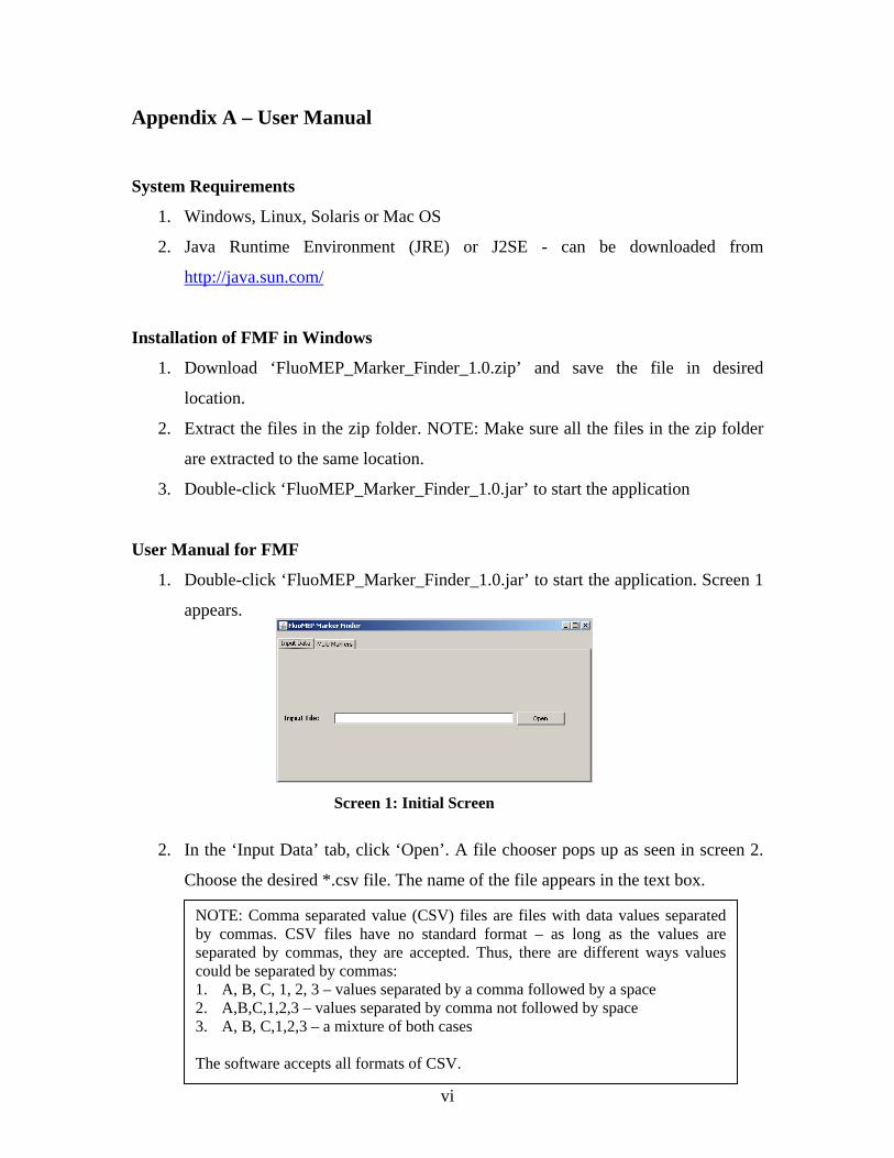
1. Double-click ‘FluoMEP_Marker_Finder_1.0.jar’ to start the application. Screen 1
appears.
2. In the ‘Input Data’ tab, click ‘Open’. A file chooser pops up as seen in screen 2.
Choose the desired *.csv file. The name of the file appears in the text box.
Screen 1: Initial Screen
NOTE: Comma separated value (CSV) files are files with data values separated by commas. CSV files have no standard format – as long as the values are separated by commas, they are accepted. Thus, there are different ways values could be separated by commas: 1. A, B, C, 1, 2, 3 – values separated by a comma followed by a space 2. A,B,C,1,2,3 – values separated by comma not followed by space 3. A, B, C,1,2,3 – a mixture of both cases The software accepts all formats of CSV.
vii
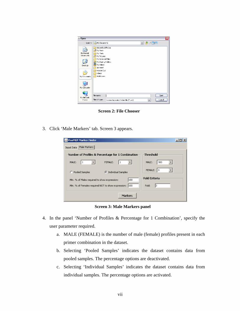
3. Click ‘Male Markers’ tab. Screen 3 appears.
4. In the panel ‘Number of Profiles & Percentage for 1 Combination’, specify the
user parameter required.
a. MALE (FEMALE) is the number of male (female) profiles present in each
primer combination in the dataset.
b. Selecting ‘Pooled Samples’ indicates the dataset contains data from
pooled samples. The percentage options are deactivated.
c. Selecting ‘Individual Samples’ indicates the dataset contains data from
individual samples. The percentage options are activated.
Screen 2: File Chooser
Screen 3: Male Markers panel

viii
d. Min. percentage of males required to show expression is the minimum
number of male samples required (in percentage) to show presence of a
peak, for the peak to be considered a male marker. For pooled samples,
this option is deactivated and a default value of 100% is used.
e. Min. percentage of females required not to show expression is the
minimum number of female samples not required (in percentage) to show
presence of a peak, for the peak to be considered a male marker. For
pooled samples, this option is deactivated and a default value of 100% is
used.
5. In the ‘Threshold’ panel, the minimum peak height filter is set. For males, a
default of 300 rfu is set. Thus, male peaks below height of 300 rfu are rejected.
For females, a default of 0 rfu is set as all female peaks are considered for
comparison against males.
6. In the ‘Fold’ panel, the minimum factor the male peak heights must be greater
than the female peak heights to be considered a marker. The default setting is 3,
i.e. a male peak height must be at least 3 times higher than the corresponding
female peak height to be considered a marker.
7. Click Markers to analyze. Output file appears in same destination as input file
with name: input_filename_malemarkers.csv.
Things to Note
1. All input files must contain the three columns ‘Sample File Name’, ‘Size’ and
‘Height’. If the other columns (Dye/Sample Peak, Marker, Allele, Area and Data
Point) are present in the file, then they must appear in the following order:
Dye/Sample Peak, Sample File Name, Marker, Allele, Size, Height, Area, Data
point.
2. Troubleshooting for JAR files: http://www.netbeans.org/kb/articles/javase-
deploy.html