Computational Mechanics Research and Support for ... · Computational Mechanics Research and Support for Aerodynamics and Hydraulics at TFHRC, Year 3 Quarter 1 Progress Report by

Computational Mechanics Research and Support

for Aerodynamics and Hydraulics at TFHRC

ANL/ESD/13-2

Year 3 Quarter 1 Progress Report

Disclaimer This report was prepared as an account of work sponsored by an agency of the United States Government. Neither the United States Government nor any agency thereof, nor UChicago Argonne, LLC, nor any of their employees or officers, makes any warranty, express or implied, or assumes any legal liability or responsibility for the accuracy, completeness, or usefulness of any information, apparatus, product, or process disclosed, or represents that its use would not infringe privately owned rights. Reference herein to any specific commercial product, process, or service by trade name, trademark, manufacturer, or otherwise, does not necessarily constitute or imply its endorsement, recommendation, or favoring by the United States Government or any agency thereof. The views and opinions of document authors expressed herein do not necessarily state or reflect those of the United States Government or any agency thereof, Argonne National Laboratory, or UChicago Argonne, LLC.

Availability of This Report This report is available, at no cost, at http://www.osti.gov/bridge. It is also available on paper to the U.S. Department of Energy and its contractors, for a processing fee, from:

U.S. Department of Energy Office of Scientific and Technical Information P.O. Box 62 Oak Ridge, TN 37831-0062 phone (865) 576-8401 fax (865) 576-5728

[email protected]

About Argonne National Laboratory

Argonne is a U.S. Department of Energy laboratory managed by UChicago Argonne, LLC

under contract DE-AC02-06CH11357. The Laboratory’s main facility is outside Chicago,

at 9700 South Cass Avenue, Argonne, Illinois 60439. For information about Argonne

and its pioneering science and technology programs, see www.anl.gov.

Computational Mechanics Research and Support for Aerodynamics and Hydraulics at TFHRC, Year 3 Quarter 1 Progress Report

by S.A. Lottes1, C. Bojanowski1 1 Transportation Research and Analysis Computing Center (TRACC) Energy Systems Division, Argonne National Laboratory submitted to Kornel Kerenyi1 and Harold Bosch1 1 Turner-Fairbank Highway Research Center May 2013

ANL/ESD/13-2

TRACC/TFHRC Y3Q1 Page 3

Table of Contents

1. Introduction and Objectives ................................................................................................................. 8

1.1. Hydraulics Modeling and Analysis Summary ................................................................................... 9

1.2. Wind Engineering Modeling and Analysis Summary ....................................................................... 9

1.3. Weathering Steel Modeling and Analysis Summary ...................................................................... 10

1.4. Technology Transfer and Facility and User Support ...................................................................... 10

2. Hydraulics Modeling and Analysis ...................................................................................................... 11

2.1. Modeling of Flow through Grates .................................................................................................. 11

2.2. Modeling of Flow through Slots in Highway Road Barriers ........................................................... 19

2.3. Onset of Rip-Rap Motion using STAR-CCM+ Coupled with LS-DYNA............................................. 23

3. Wind Engineering Modeling and Analysis........................................................................................... 26

3.1. Analysis of Sign Vibration Due to Passing Trucks ........................................................................... 26

4. Weathering Steel Truck Spray Modeling and Analysis ....................................................................... 35

4.1. Depressed Grade Approach Effect Study ....................................................................................... 35

5. Technology Transfer ........................................................................................................................... 38

6. TRACC Facility and User Support for TFHRC ....................................................................................... 39


List of Figures

Figure 2.1 Grate design without vanes ....................................................................................................... 11

Figure 2.2 Grate design with vanes ............................................................................................................. 11

Figure 2.3 Computational domain for testing flow interception by grate .................................................. 12

Figure 2.4 Cross section of the computational mesh for grate with vanes model ..................................... 12

Figure 2.5 Water volume fraction showing free surface location on vertical slice through grate without

vanes at 7s .................................................................................................................................................. 13

Figure 2.6 Water volume fraction showing free surface location on vertical slice through grate with

vanes at 7 s .................................................................................................................................................. 13

Figure 2.7 3-D visualization of water free surface over grate without vanes at 7 s ................................... 13

Figure 2.8 3-D visualization of water free surface over grate with vanes at 7 s ......................................... 14

Figure 2.9 Development of volume flow past the grates ........................................................................... 14

Figure 2.10 Development of volume flow captured by the grates ............................................................. 15

Figure 2.11 Exaggerated simple street cross section geometry ................................................................. 16

Figure 2.12 Cross section of street and gutter with different slopes ......................................................... 16

Figure 2.13 Volume fraction of water on two slices along and across street ............................................. 18

Figure 2.14 Velocity on two slices along and across street ........................................................................ 19

Figure 2.15 Road barrier schematic ............................................................................................................ 19

Figure 2.16 Computational domain for road barrier drainage analysis ...................................................... 20

Figure 2.17 Stream wise and cross stream vertical slices through the domain showing the computational

mesh ............................................................................................................................................................ 21

Figure 2.18 Flow rate of water through openings in a road barrier when there is no water in the street

initially and the 0.13 m (5 in) deep, 2 m/s water flow is started at time zero ........................................... 21

Figure 2.19 3D visualization of free surface at three times as water moves past street barrier ............... 22

Figure 2.20 Point cloud and triangulated surface of scanned rock ............................................................ 23


Figure 2.21 Different rock shapes created in MeshLab; The green rock was scanned others were derived

from it ......................................................................................................................................................... 23

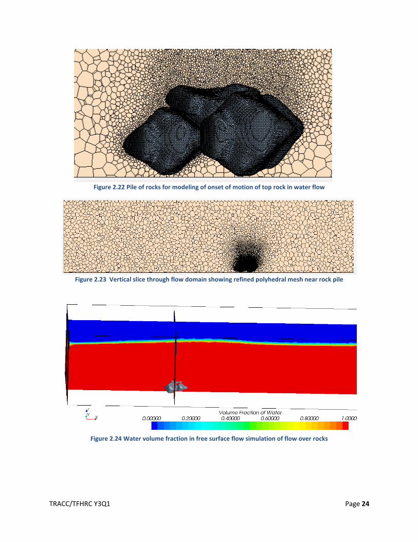
Figure 2.22 Pile of rocks for modeling of onset of motion of top rock in water flow ................................ 24

Figure 2.23 Vertical slice through flow domain showing refined polyhedral mesh near rock pile ........... 24

Figure 2.24 Water volume fraction in free surface flow simulation of flow over rocks ............................. 24

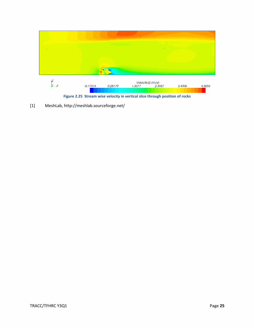
Figure 2.25 Stream wise velocity in vertical slice through position of rocks ............................................. 25

Figure 3.1 Modeled over highway sign support structure and sign enclosure ........................................... 26

Figure 3.2 A slice through the computational domain ............................................................................... 27

Figure 3.3 Pressure distribution on sign during passage of a truck ............................................................ 28

Figure 3.4 Close up view on the sign with pressure distribution during passage of a truck ...................... 28

Figure 3.5 Pressure plot at point of maximum pressure ............................................................................ 29

Figure 3.6 Vibration of the sign due to the passage of one truck measured at the point farthest out over

the road ....................................................................................................................................................... 29

Figure 3.7 Maximum pressure signature of a string of 20 trucks passing .................................................. 30

Figure 3.8 Trucks without and with over cab flow diverter ........................................................................ 30

Figure 3.9 Elements monitored for pressure history .................................................................................. 31

Figure 3.10 Pressure at front monitor point for truck with aerodynamic cab ........................................... 31

Figure 3.11 Pressure at bottom monitoring point for truck with aerodynamic cab .................................. 32

Figure 3.12 Pressure at front monitor point for truck with non-aerodynamic cab .................................... 32

Figure 3.13 Pressure at bottom monitoring point for truck with non-aerodynamic cab ........................... 33

Figure 3.14 Vertical vibration due to the passage of 3 old style trucks with non-aerodynamic cabs ........ 33

Figure 3.15 Vertical vibration due to the passage of 20 old style trucks with non-aerodynamic cabs ...... 34

Figure 4.1: Depressed grade bridge approach with vertical abutments .................................................... 35

Figure 4.2: An example of a long depressed grade approach to a bridge with vertical walls .................... 35

Figure 4.3: Geometry of the bridge with extreme depressed approach with vertical walls on both sides of

the roadway creating a cavity in the terrain near the bridge ..................................................................... 36


Figure 4.4: Cumulative plot presenting number of parcels at the bridge girder level for simulations with

tunnel conditions ........................................................................................................................................ 37

Figure 4.5: Flow induced in the tunnel causing transport of increased number of salt spray parcels to the

bridge girder level ....................................................................................................................................... 37


List of Tables

Table 2.1 Street Flow Test Conditions ........................................................................................................ 18


1. Introduction and Objectives

The computational fluid dynamics (CFD) and computational structural mechanics (CSM) focus areas at

Argonne’s Transportation Research and Analysis Computing Center (TRACC) initiated a project to

support and compliment the experimental programs at the Turner-Fairbank Highway Research Center

(TFHRC) with high performance computing based analysis capabilities in August 2010. The project was

established with a new interagency agreement between the Department of Energy and the Department

of Transportation to provide collaborative research, development, and benchmarking of advanced

three-dimensional computational mechanics analysis methods to the aerodynamics and hydraulics

laboratories at TFHRC for a period of five years, beginning in October 2010. The analysis methods

employ well benchmarked and supported commercial computational mechanics software.

Computational mechanics encompasses the areas of Computational Fluid Dynamics (CFD),

Computational Wind Engineering (CWE), Computational Structural Mechanics (CSM), and Computational

Multiphysics Mechanics (CMM) applied in Fluid-Structure Interaction (FSI) problems.

The major areas of focus of the project are wind and water effects on bridges — superstructure, deck,

cables, and substructure (including soil), primarily during storms and flood events — and the risks that

these loads pose to structural failure. For flood events at bridges, another major focus of the work is

assessment of the risk to bridges caused by scour of stream and riverbed material away from the

foundations of a bridge. Other areas of current research include modeling of the salt spray transport

into bridge girders to address suitability of using weathering steel in bridges, CFD analysis of the

operation of the wind tunnel in the TFHRC wind engineering laboratory, and coupling of CFD and CSM

software to solve fluid structure interaction problems, primarily analysis of bridge cables in wind.

This quarterly report documents technical progress on the project tasks for the period of October

through December 2012.


1.1. Hydraulics Modeling and Analysis Summary

The primary Computational Fluid Dynamics (CFD) activities during the quarter focused on new modeling

efforts including calculating the fraction street storm water intercepted by two different drain grate

designs, modeling of storm water past and through the slots in temporary street barriers, and the onset

of motion of large pieces of rip-rap. Modeling the fraction of flow intercepted by drain grates was done

as a test of capability of the VOF free surface model and use of pressure outlet boundary conditions to

allow the computation of the flow split among multiple outlets. The free surface of the street level flow

is well broken up when a portion of the flow is pulled by gravity through the grate. The VOF model loses

accuracy when the free surface is not intact, however the tests confirmed that mass balance is still well

preserved in this model, and consequently the fraction of the flow intercepted by the drain can be

computed with engineering accuracy. Details are provided in Section 2.1. Modeling of flow intercepted

by the slots on the bottom of temporary street barriers was tested at the request of a state DOT and is

covered in Section 2.2. The model was built from the street drain model by replacing the drain and catch

basin with a street barrier. This model appears to function well.

The development of a methodology to model the onset of motion of large irregular rocks in rip-rap was

begun. The model was designed to have a high fidelity and include the force distribution of the surface

of a rock. STAR-CCM+ has the capability to model dynamic fluid body interaction (DFBI) problems when

the bodies are not in contact with each other. In the case of rip-rap, the rocks on the top are in contact

with the underlying layer of rocks and therefore the DFBI model cannot be used. The fluid structure

interaction (FSI) capability recently in development between STAR-CCM+ and LS-DYNA was chosen for

development of this model. LS-DYNA can compute rigid body motion based on the flow generated force

distribution passed to it from CFD computation. Then LS-DYNA can pass back displacements of the rock

surface to STAR-CCM+ for mesh morphing. LS-DYNA is also used to compute collisions of rock surfaces

and prevents rock boundaries from intersecting other solid boundaries. Additional details can be found

in Section 2.3.

1.2. Wind Engineering Modeling and Analysis Summary

The effort in wind engineering began model development for analysis of truck passing induced

vibrations in over highway Variable Message Signs (VMS). Large vibrations have been observed in some

existing signs and a model that can be used to investigate causes and conditions for excessive sign

vibration is desired. This model can use previous efforts in modeling trucks passing under bridges using

the sliding mesh capabilities of STAR-CCM+ CFD software and the FSI capabilities being developed to

model bridge cable vibration. Details of the effort to build the model and initial testing are in Section

3.1.


1.3. Weathering Steel Modeling and Analysis Summary

An additional case geometry was analyzed for salt laden droplet transport from trucks to bridge girders

to assess corrosion risk for weathering steel bridges. The geometry is that of long depressed grade

approach with vertical retaining walls flanking the road on both sides. This type of approach forms a slot

cavity in the terrain, and when wind blows across it at the level of the surrounding terrain, recirculation

zones with wind up drafts can be generated in the depressed approach cavity. Simulations with 10 mph

and 30 mph cross winds indicate that with this geometry and the tested wind conditions large numbers

of droplet parcels can be transported to girder level.

1.4. Technology Transfer and Facility and User Support

Plans were made for visiting TFHRC during TRB week in January, allowing for both a project meeting

with updates on the experimental facilities at TFHRC and attendance at hydraulic committee meetings

during the TRB meeting. The new Zephyr cluster became available for general production use, and

procedures for using it were added to the TRACC wiki. Bi-weekly videoconferences with TFHRC and

other collaborators were continued through the quarter.


2. Hydraulics Modeling and Analysis

2.1. Modeling of Flow through Grates

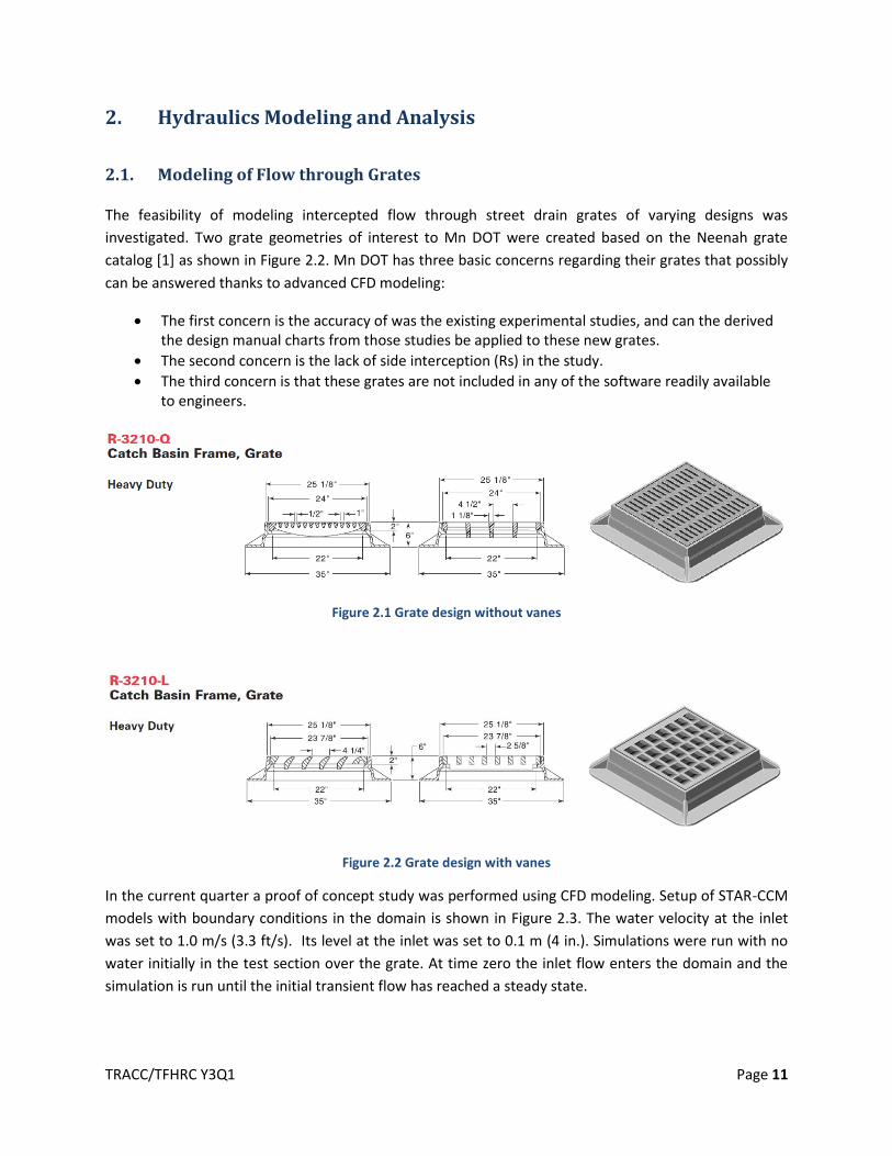
The feasibility of modeling intercepted flow through street drain grates of varying designs was

investigated. Two grate geometries of interest to Mn DOT were created based on the Neenah grate

catalog [1] as shown in Figure 2.2. Mn DOT has three basic concerns regarding their grates that possibly

can be answered thanks to advanced CFD modeling:

The first concern is the accuracy of was the existing experimental studies, and can the derived the design manual charts from those studies be applied to these new grates.

The second concern is the lack of side interception (Rs) in the study.

The third concern is that these grates are not included in any of the software readily available to engineers.

Figure 2.1 Grate design without vanes

Figure 2.2 Grate design with vanes

In the current quarter a proof of concept study was performed using CFD modeling. Setup of STAR-CCM

models with boundary conditions in the domain is shown in Figure 2.3. The water velocity at the inlet

was set to 1.0 m/s (3.3 ft/s). Its level at the inlet was set to 0.1 m (4 in.). Simulations were run with no

water initially in the test section over the grate. At time zero the inlet flow enters the domain and the

simulation is run until the initial transient flow has reached a steady state.


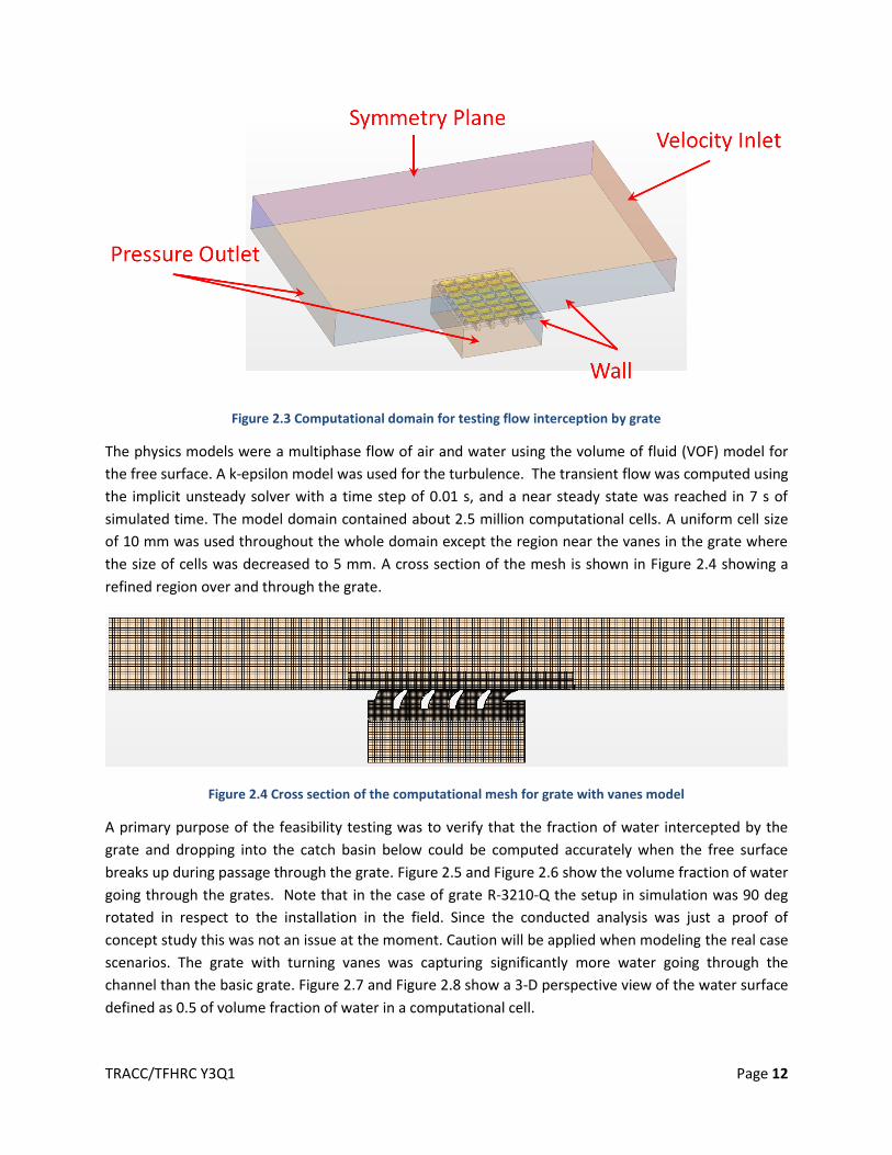
Figure 2.3 Computational domain for testing flow interception by grate

The physics models were a multiphase flow of air and water using the volume of fluid (VOF) model for

the free surface. A k-epsilon model was used for the turbulence. The transient flow was computed using

the implicit unsteady solver with a time step of 0.01 s, and a near steady state was reached in 7 s of

simulated time. The model domain contained about 2.5 million computational cells. A uniform cell size

of 10 mm was used throughout the whole domain except the region near the vanes in the grate where

the size of cells was decreased to 5 mm. A cross section of the mesh is shown in Figure 2.4 showing a

refined region over and through the grate.

Figure 2.4 Cross section of the computational mesh for grate with vanes model

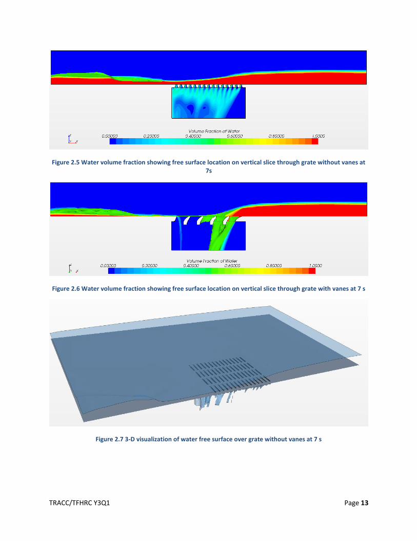
A primary purpose of the feasibility testing was to verify that the fraction of water intercepted by the

grate and dropping into the catch basin below could be computed accurately when the free surface

breaks up during passage through the grate. Figure 2.5 and Figure 2.6 show the volume fraction of water

going through the grates. Note that in the case of grate R-3210-Q the setup in simulation was 90 deg

rotated in respect to the installation in the field. Since the conducted analysis was just a proof of

concept study this was not an issue at the moment. Caution will be applied when modeling the real case

scenarios. The grate with turning vanes was capturing significantly more water going through the

channel than the basic grate. Figure 2.7 and Figure 2.8 show a 3-D perspective view of the water surface

defined as 0.5 of volume fraction of water in a computational cell.


Figure 2.5 Water volume fraction showing free surface location on vertical slice through grate without vanes at 7s

Figure 2.6 Water volume fraction showing free surface location on vertical slice through grate with vanes at 7 s

Figure 2.7 3-D visualization of water free surface over grate without vanes at 7 s


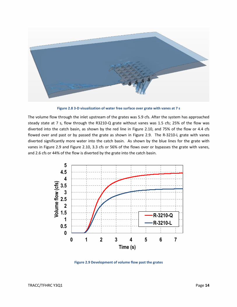
Figure 2.8 3-D visualization of water free surface over grate with vanes at 7 s

The volume flow through the inlet upstream of the grates was 5.9 cfs. After the system has approached

steady state at 7 s, flow through the R3210-Q grate without vanes was 1.5 cfs; 25% of the flow was

diverted into the catch basin, as shown by the red line in Figure 2.10, and 75% of the flow or 4.4 cfs

flowed over and past or by passed the grate as shown in Figure 2.9. The R-3210-L grate with vanes

diverted significantly more water into the catch basin. As shown by the blue lines for the grate with

vanes in Figure 2.9 and Figure 2.10, 3.3 cfs or 56% of the flows over or bypasses the grate with vanes,

and 2.6 cfs or 44% of the flow is diverted by the grate into the catch basin.

Figure 2.9 Development of volume flow past the grates

0

0.5

1

1.5

2

2.5

3

3.5

4

4.5

5

0 1 2 3 4 5 6 7

Vo

lum

e fl

ow

(cf

s)

Time (s)

R-3210-Q

R-3210-L


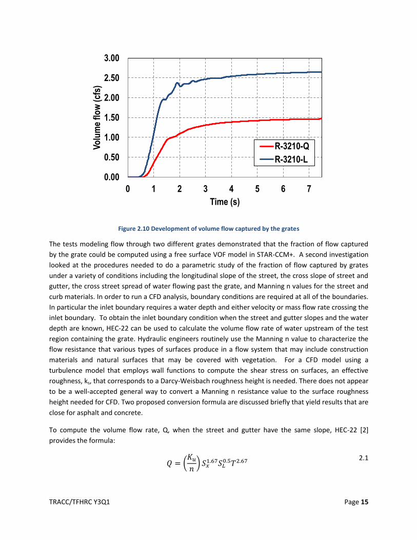
Figure 2.10 Development of volume flow captured by the grates

The tests modeling flow through two different grates demonstrated that the fraction of flow captured

by the grate could be computed using a free surface VOF model in STAR-CCM+. A second investigation

looked at the procedures needed to do a parametric study of the fraction of flow captured by grates

under a variety of conditions including the longitudinal slope of the street, the cross slope of street and

gutter, the cross street spread of water flowing past the grate, and Manning n values for the street and

curb materials. In order to run a CFD analysis, boundary conditions are required at all of the boundaries.

In particular the inlet boundary requires a water depth and either velocity or mass flow rate crossing the

inlet boundary. To obtain the inlet boundary condition when the street and gutter slopes and the water

depth are known, HEC-22 can be used to calculate the volume flow rate of water upstream of the test

region containing the grate. Hydraulic engineers routinely use the Manning n value to characterize the

flow resistance that various types of surfaces produce in a flow system that may include construction

materials and natural surfaces that may be covered with vegetation. For a CFD model using a

turbulence model that employs wall functions to compute the shear stress on surfaces, an effective

roughness, ks, that corresponds to a Darcy-Weisbach roughness height is needed. There does not appear

to be a well-accepted general way to convert a Manning n resistance value to the surface roughness

height needed for CFD. Two proposed conversion formula are discussed briefly that yield results that are

close for asphalt and concrete.

To compute the volume flow rate, Q, when the street and gutter have the same slope, HEC-22 [2]

provides the formula:

(

)

2.1

0.00

0.50

1.00

1.50

2.00

2.50

3.00

0 1 2 3 4 5 6 7

Vo

lum

e fl

ow

(cf

s)

Time (s)

R-3210-Q

R-3210-L


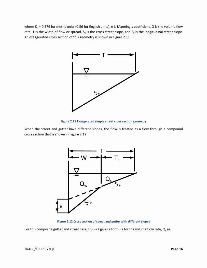
where Ku = 0.376 for metric units (0.56 for English units), n is Manning’s coefficient, Q is the volume flow

rate, T is the width of flow or spread, Sx is the cross street slope, and SL is the longitudinal street slope.

An exaggerated cross section of this geometry is shown in Figure 2.11

Figure 2.11 Exaggerated simple street cross section geometry

When the street and gutter have different slopes, the flow is treated as a flow through a compound

cross section that is shown in Figure 2.12.

Figure 2.12 Cross section of street and gutter with different slopes

For this composite gutter and street case, HEC-22 gives a formula for the volume flow rate, Q, as:

Ts

Qs Qw

W

a

T

T


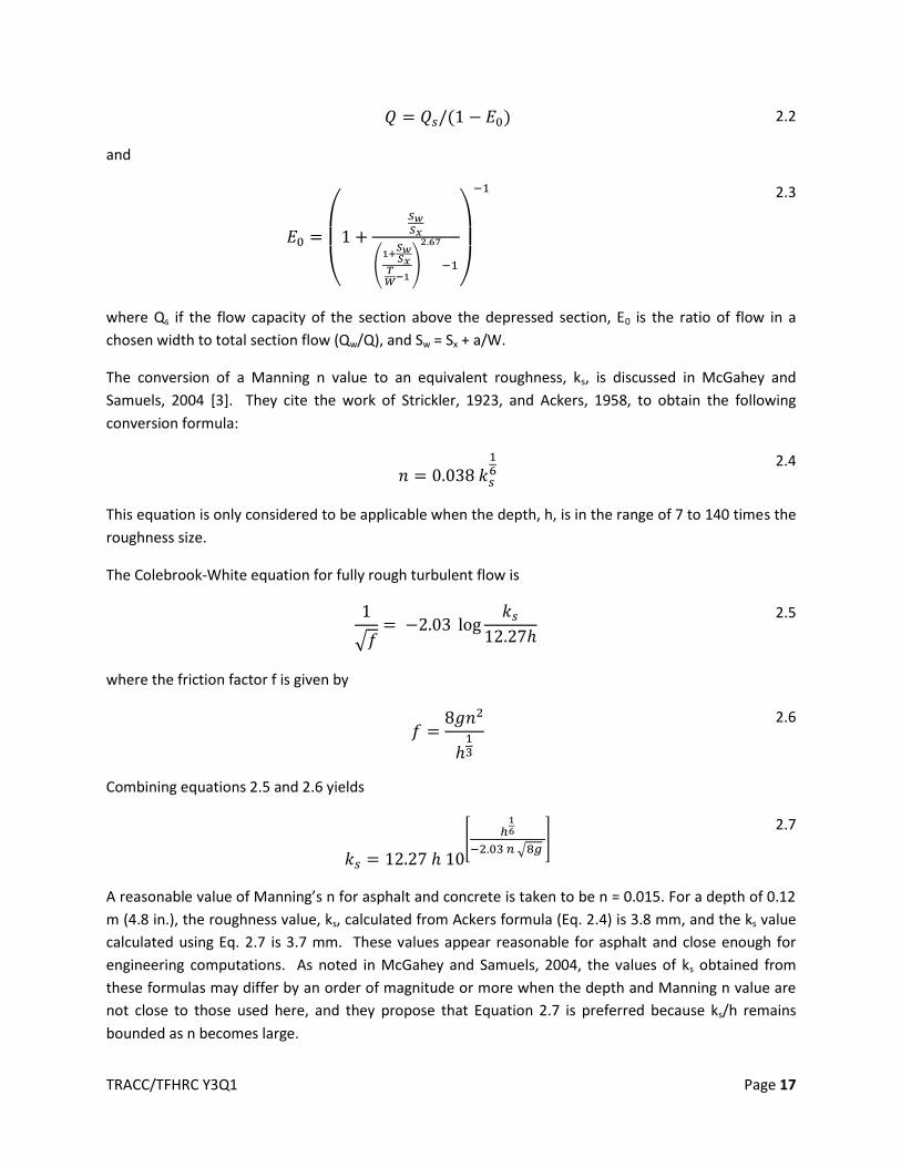
2.2

and

(

(

)

)

2.3

where Qs if the flow capacity of the section above the depressed section, E0 is the ratio of flow in a

chosen width to total section flow (Qw/Q), and Sw = Sx + a/W.

The conversion of a Manning n value to an equivalent roughness, ks, is discussed in McGahey and

Samuels, 2004 [3]. They cite the work of Strickler, 1923, and Ackers, 1958, to obtain the following

conversion formula:

2.4

This equation is only considered to be applicable when the depth, h, is in the range of 7 to 140 times the

roughness size.

The Colebrook-White equation for fully rough turbulent flow is

√

2.5

where the friction factor f is given by

2.6

Combining equations 2.5 and 2.6 yields

[

√ ]

2.7

A reasonable value of Manning’s n for asphalt and concrete is taken to be n = 0.015. For a depth of 0.12

m (4.8 in.), the roughness value, ks, calculated from Ackers formula (Eq. 2.4) is 3.8 mm, and the ks value

calculated using Eq. 2.7 is 3.7 mm. These values appear reasonable for asphalt and close enough for

engineering computations. As noted in McGahey and Samuels, 2004, the values of ks obtained from

these formulas may differ by an order of magnitude or more when the depth and Manning n value are

not close to those used here, and they propose that Equation 2.7 is preferred because ks/h remains

bounded as n becomes large.


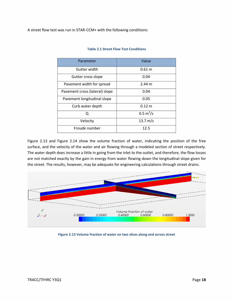
A street flow test was run in STAR-CCM+ with the following conditions:

Table 2.1 Street Flow Test Conditions

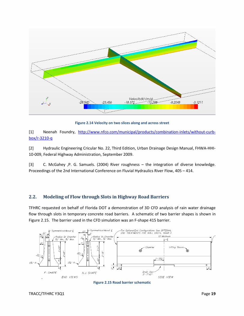
Figure 2.13 and Figure 2.14 show the volume fraction of water, indicating the position of the free

surface, and the velocity of the water and air flowing through a modeled section of street respectively.

The water depth does increase a little in going from the inlet to the outlet, and therefore, the flow losses

are not matched exactly by the gain in energy from water flowing down the longitudinal slope given for

the street. The results, however, may be adequate for engineering calculations through street drains.

Figure 2.13 Volume fraction of water on two slices along and across street

Parameter Value

Gutter width 0.61 m

Gutter cross slope 0.04

Pavement width for spread 2.44 m

Pavement cross (lateral) slope 0.04

Pavement longitudinal slope 0.05

Curb water depth 0.12 m

Q 0.5 m3/s

Velocity 13.7 m/s

Froude number 12.5


Figure 2.14 Velocity on two slices along and across street

[1] Neenah Foundry, http://www.nfco.com/municipal/products/combination-inlets/without-curb-

box/r-3210-q

[2] Hydraulic Engineering Cricular No. 22, Third Edition, Urban Drainage Design Manual, FHWA-HHI-

10-009, Federal Highway Administration, September 2009.

[3] C. McGahey ,P. G. Samuels. (2004) River roughness – the integration of diverse knowledge.

Proceedings of the 2nd International Conference on Fluvial Hydraulics River Flow, 405 – 414.

2.2. Modeling of Flow through Slots in Highway Road Barriers

TFHRC requested on behalf of Florida DOT a demonstration of 3D CFD analysis of rain water drainage

flow through slots in temporary concrete road barriers. A schematic of two barrier shapes is shown in

Figure 2.15. The barrier used in the CFD simulation was an F-shape 415 barrier.

Figure 2.15 Road barrier schematic

http://www.nfco.com/municipal/products/combination-inlets/without-curb-box/r-3210-q

http://www.nfco.com/municipal/products/combination-inlets/without-curb-box/r-3210-q


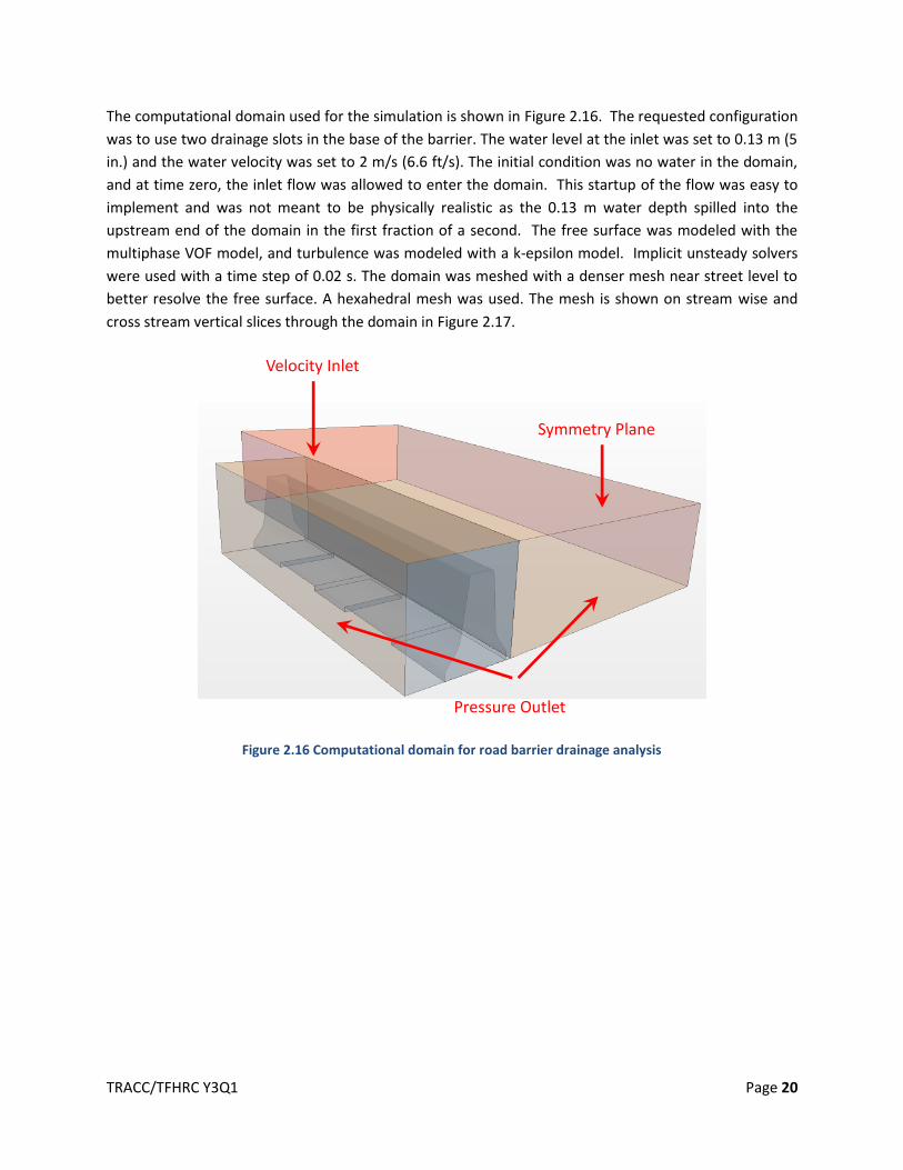
The computational domain used for the simulation is shown in Figure 2.16. The requested configuration

was to use two drainage slots in the base of the barrier. The water level at the inlet was set to 0.13 m (5

in.) and the water velocity was set to 2 m/s (6.6 ft/s). The initial condition was no water in the domain,

and at time zero, the inlet flow was allowed to enter the domain. This startup of the flow was easy to

implement and was not meant to be physically realistic as the 0.13 m water depth spilled into the

upstream end of the domain in the first fraction of a second. The free surface was modeled with the

multiphase VOF model, and turbulence was modeled with a k-epsilon model. Implicit unsteady solvers

were used with a time step of 0.02 s. The domain was meshed with a denser mesh near street level to

better resolve the free surface. A hexahedral mesh was used. The mesh is shown on stream wise and

cross stream vertical slices through the domain in Figure 2.17.

Figure 2.16 Computational domain for road barrier drainage analysis

Velocity Inlet

Symmetry Plane

Pressure Outlet


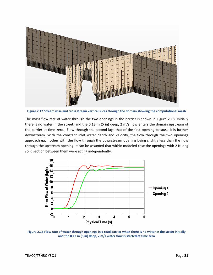
Figure 2.17 Stream wise and cross stream vertical slices through the domain showing the computational mesh

The mass flow rate of water through the two openings in the barrier is shown in Figure 2.18. Initially

there is no water in the street, and the 0.13 m (5 in) deep, 2 m/s flow enters the domain upstream of

the barrier at time zero. Flow through the second lags that of the first opening because it is further

downstream. With the constant inlet water depth and velocity, the flow through the two openings

approach each other with the flow through the downstream opening being slightly less than the flow

through the upstream opening. It can be assumed that within modeled case the openings with 2 ft long

solid section between them were acting independently.

Figure 2.18 Flow rate of water through openings in a road barrier when there is no water in the street initially and the 0.13 m (5 in) deep, 2 m/s water flow is started at time zero


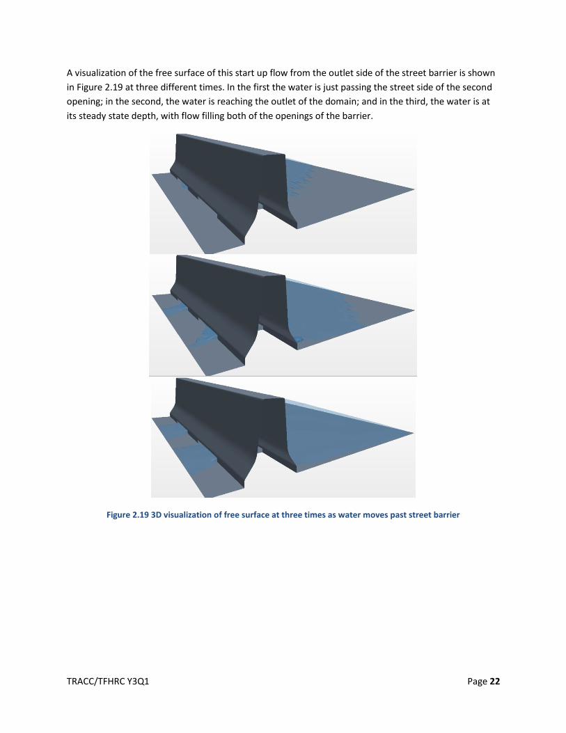
A visualization of the free surface of this start up flow from the outlet side of the street barrier is shown

in Figure 2.19 at three different times. In the first the water is just passing the street side of the second

opening; in the second, the water is reaching the outlet of the domain; and in the third, the water is at

its steady state depth, with flow filling both of the openings of the barrier.

Figure 2.19 3D visualization of free surface at three times as water moves past street barrier


2.3. Onset of Rip-Rap Motion using STAR-CCM+ Coupled with LS-DYNA

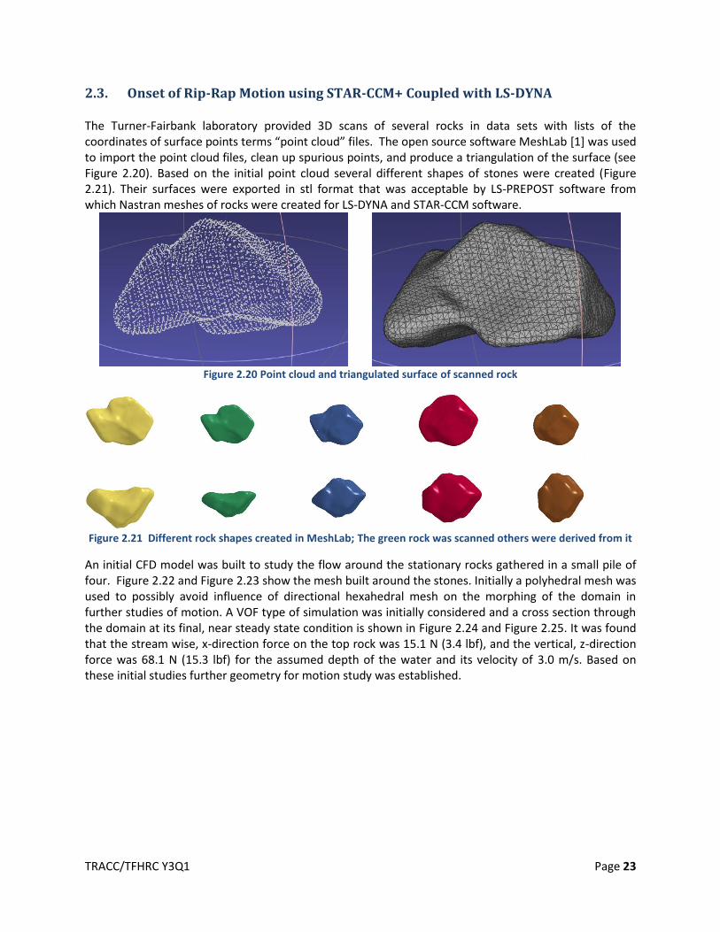
The Turner-Fairbank laboratory provided 3D scans of several rocks in data sets with lists of the coordinates of surface points terms “point cloud” files. The open source software MeshLab [1] was used to import the point cloud files, clean up spurious points, and produce a triangulation of the surface (see Figure 2.20). Based on the initial point cloud several different shapes of stones were created (Figure 2.21). Their surfaces were exported in stl format that was acceptable by LS-PREPOST software from which Nastran meshes of rocks were created for LS-DYNA and STAR-CCM software.

Figure 2.20 Point cloud and triangulated surface of scanned rock

Figure 2.21 Different rock shapes created in MeshLab; The green rock was scanned others were derived from it

An initial CFD model was built to study the flow around the stationary rocks gathered in a small pile of four. Figure 2.22 and Figure 2.23 show the mesh built around the stones. Initially a polyhedral mesh was used to possibly avoid influence of directional hexahedral mesh on the morphing of the domain in further studies of motion. A VOF type of simulation was initially considered and a cross section through the domain at its final, near steady state condition is shown in Figure 2.24 and Figure 2.25. It was found that the stream wise, x-direction force on the top rock was 15.1 N (3.4 lbf), and the vertical, z-direction force was 68.1 N (15.3 lbf) for the assumed depth of the water and its velocity of 3.0 m/s. Based on these initial studies further geometry for motion study was established.


Figure 2.22 Pile of rocks for modeling of onset of motion of top rock in water flow

Figure 2.23 Vertical slice through flow domain showing refined polyhedral mesh near rock pile

Figure 2.24 Water volume fraction in free surface flow simulation of flow over rocks


Figure 2.25 Stream wise velocity in vertical slice through position of rocks

[1] MeshLab, http://meshlab.sourceforge.net/


3. Wind Engineering Modeling and Analysis

3.1. Analysis of Sign Vibration Due to Passing Trucks

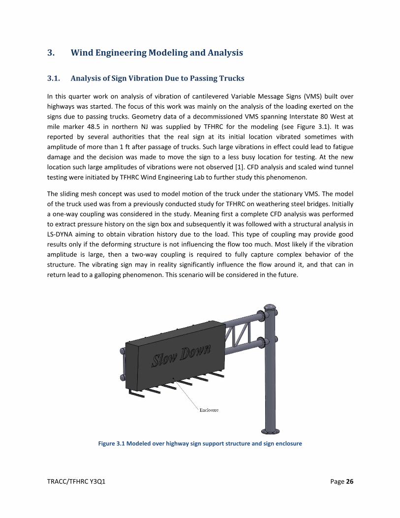
In this quarter work on analysis of vibration of cantilevered Variable Message Signs (VMS) built over

highways was started. The focus of this work was mainly on the analysis of the loading exerted on the

signs due to passing trucks. Geometry data of a decommissioned VMS spanning Interstate 80 West at

mile marker 48.5 in northern NJ was supplied by TFHRC for the modeling (see Figure 3.1). It was

reported by several authorities that the real sign at its initial location vibrated sometimes with

amplitude of more than 1 ft after passage of trucks. Such large vibrations in effect could lead to fatigue

damage and the decision was made to move the sign to a less busy location for testing. At the new

location such large amplitudes of vibrations were not observed [1]. CFD analysis and scaled wind tunnel

testing were initiated by TFHRC Wind Engineering Lab to further study this phenomenon.

The sliding mesh concept was used to model motion of the truck under the stationary VMS. The model

of the truck used was from a previously conducted study for TFHRC on weathering steel bridges. Initially

a one-way coupling was considered in the study. Meaning first a complete CFD analysis was performed

to extract pressure history on the sign box and subsequently it was followed with a structural analysis in

LS-DYNA aiming to obtain vibration history due to the load. This type of coupling may provide good

results only if the deforming structure is not influencing the flow too much. Most likely if the vibration

amplitude is large, then a two-way coupling is required to fully capture complex behavior of the

structure. The vibrating sign may in reality significantly influence the flow around it, and that can in

return lead to a galloping phenomenon. This scenario will be considered in the future.

Figure 3.1 Modeled over highway sign support structure and sign enclosure


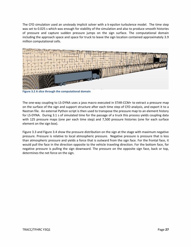
The CFD simulation used an unsteady implicit solver with a k-epsilon turbulence model. The time step was set to 0.025 s which was enough for stability of the simulation and also to produce smooth histories of pressure and capture sudden pressure jumps on the sign surface. The computational domain including the approach space and space for truck to leave the sign location contained approximately 3.9 million computational cells.

Figure 3.2 A slice through the computational domain

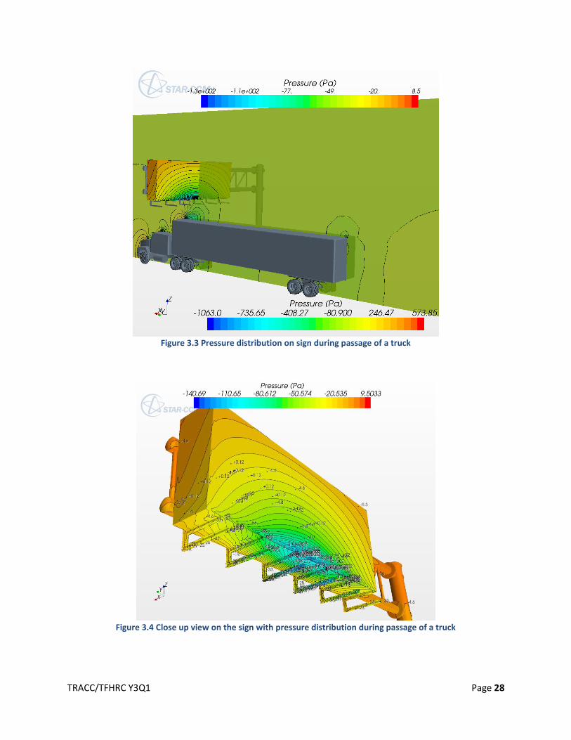
The one-way coupling to LS-DYNA uses a java macro executed in STAR-CCM+ to extract a pressure map on the surface of the sign and support structure after each time step of CFD analysis, and export it to a Nastran file. An external Python script is then used to transpose the pressure map to an element history for LS-DYNA. During 3.1 s of simulated time for the passage of a truck this process yields coupling data with 125 pressure maps (one per each time step) and 7,500 pressure histories (one for each surface element on the sign box). Figure 3.3 and Figure 3.4 show the pressure distribution on the sign at the stage with maximum negative pressure. Pressure is relative to local atmospheric pressure. Negative pressure is pressure that is less than atmospheric pressure and yields a force that is outward from the sign face. For the frontal face, it would pull the face in the direction opposite to the vehicle traveling direction. For the bottom face, for negative pressure is pulling the sign downward. The pressure on the opposite sign face, back or top, determines the net force on the sign.


Figure 3.3 Pressure distribution on sign during passage of a truck

Figure 3.4 Close up view on the sign with pressure distribution during passage of a truck


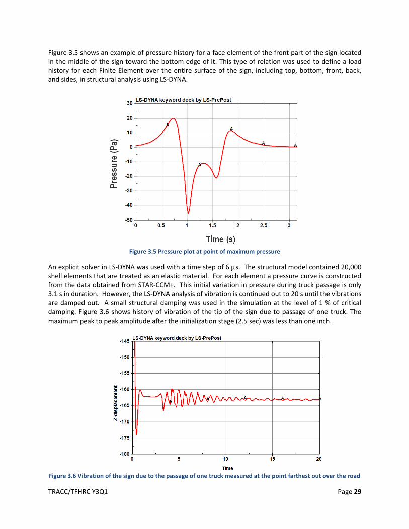
Figure 3.5 shows an example of pressure history for a face element of the front part of the sign located in the middle of the sign toward the bottom edge of it. This type of relation was used to define a load history for each Finite Element over the entire surface of the sign, including top, bottom, front, back, and sides, in structural analysis using LS-DYNA.

Figure 3.5 Pressure plot at point of maximum pressure

An explicit solver in LS-DYNA was used with a time step of 6 s. The structural model contained 20,000 shell elements that are treated as an elastic material. For each element a pressure curve is constructed from the data obtained from STAR-CCM+. This initial variation in pressure during truck passage is only 3.1 s in duration. However, the LS-DYNA analysis of vibration is continued out to 20 s until the vibrations are damped out. A small structural damping was used in the simulation at the level of 1 % of critical damping. Figure 3.6 shows history of vibration of the tip of the sign due to passage of one truck. The maximum peak to peak amplitude after the initialization stage (2.5 sec) was less than one inch.

Figure 3.6 Vibration of the sign due to the passage of one truck measured at the point farthest out over the road


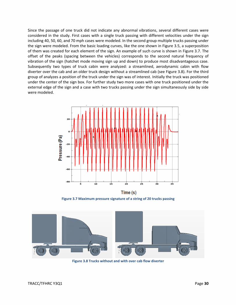
Since the passage of one truck did not indicate any abnormal vibrations, several different cases were considered in the study. First cases with a single truck passing with different velocities under the sign including 40, 50, 60, and 70 mph cases were modeled. In the second group multiple trucks passing under the sign were modeled. From the basic loading curves, like the one shown in Figure 3.5, a superposition of them was created for each element of the sign. An example of such curve is shown in Figure 3.7. The offset of the peaks (spacing between the vehicles) corresponds to the second natural frequency of vibration of the sign (hatchet mode moving sign up and down) to produce most disadvantageous case. Subsequently two types of truck cabin were analyzed: a streamlined, aerodynamic cabin with flow diverter over the cab and an older truck design without a streamlined cab (see Figure 3.8). For the third group of analyzes a position of the truck under the sign was of interest. Initially the truck was positioned under the center of the sign box. For further study two more cases with one truck positioned under the external edge of the sign and a case with two trucks passing under the sign simultaneously side by side were modeled.

Figure 3.7 Maximum pressure signature of a string of 20 trucks passing

Figure 3.8 Trucks without and with over cab flow diverter


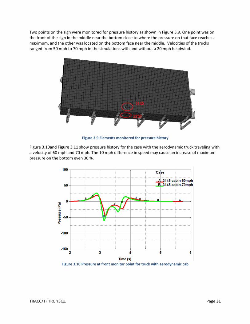
Two points on the sign were monitored for pressure history as shown in Figure 3.9. One point was on the front of the sign in the middle near the bottom close to where the pressure on that face reaches a maximum, and the other was located on the bottom face near the middle. Velocities of the trucks ranged from 50 mph to 70 mph in the simulations with and without a 20 mph headwind.

Figure 3.9 Elements monitored for pressure history

Figure 3.10and Figure 3.11 show pressure history for the case with the aerodynamic truck traveling with a velocity of 60 mph and 70 mph. The 10 mph difference in speed may cause an increase of maximum pressure on the bottom even 30 %.

Figure 3.10 Pressure at front monitor point for truck with aerodynamic cab


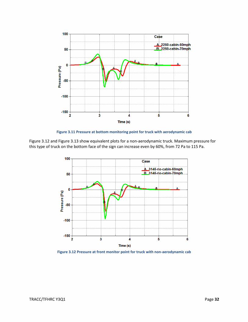
Figure 3.11 Pressure at bottom monitoring point for truck with aerodynamic cab

Figure 3.12 and Figure 3.13 show equivalent plots for a non-aerodynamic truck. Maximum pressure for this type of truck on the bottom face of the sign can increase even by 60%, from 72 Pa to 115 Pa.

Figure 3.12 Pressure at front monitor point for truck with non-aerodynamic cab


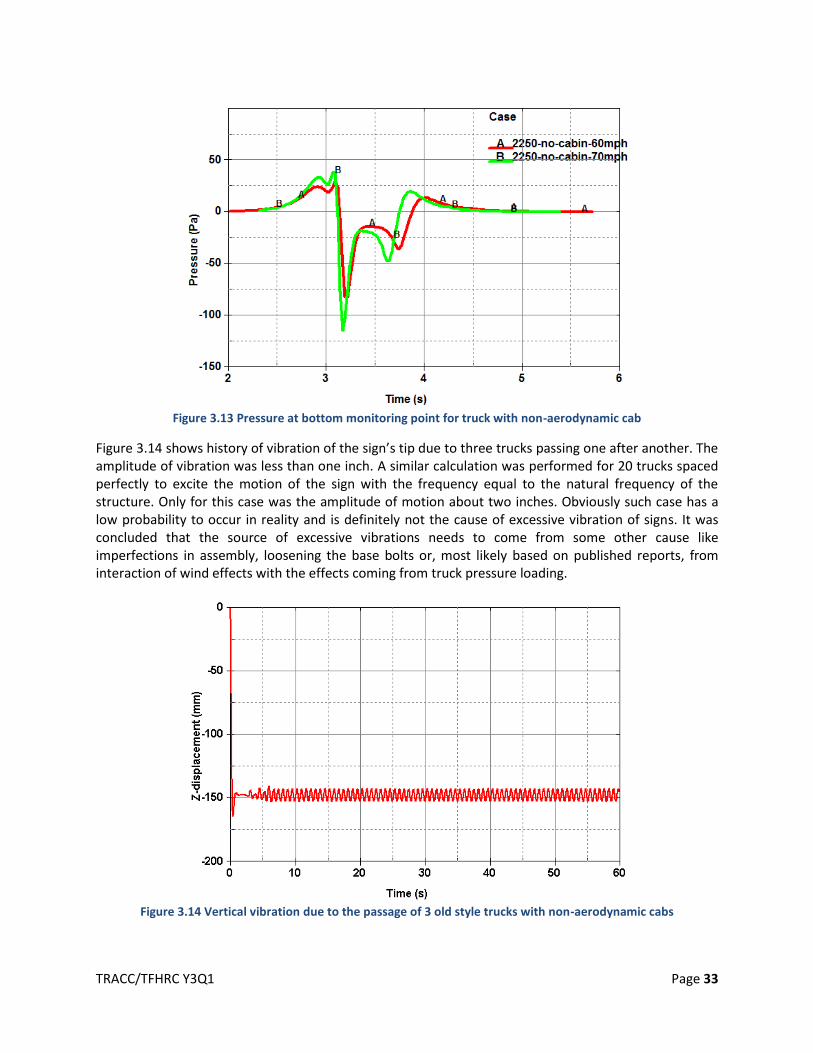
Figure 3.13 Pressure at bottom monitoring point for truck with non-aerodynamic cab

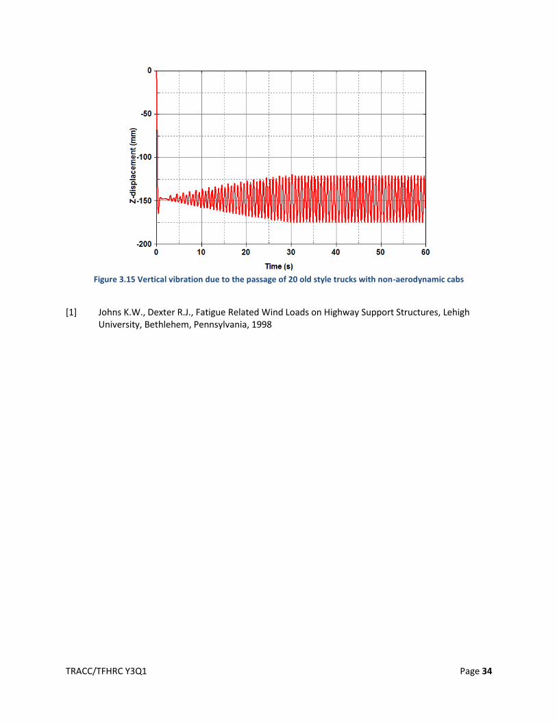
Figure 3.14 shows history of vibration of the sign’s tip due to three trucks passing one after another. The amplitude of vibration was less than one inch. A similar calculation was performed for 20 trucks spaced perfectly to excite the motion of the sign with the frequency equal to the natural frequency of the structure. Only for this case was the amplitude of motion about two inches. Obviously such case has a low probability to occur in reality and is definitely not the cause of excessive vibration of signs. It was concluded that the source of excessive vibrations needs to come from some other cause like imperfections in assembly, loosening the base bolts or, most likely based on published reports, from interaction of wind effects with the effects coming from truck pressure loading.

Figure 3.14 Vertical vibration due to the passage of 3 old style trucks with non-aerodynamic cabs


Figure 3.15 Vertical vibration due to the passage of 20 old style trucks with non-aerodynamic cabs

[1] Johns K.W., Dexter R.J., Fatigue Related Wind Loads on Highway Support Structures, Lehigh

University, Bethlehem, Pennsylvania, 1998


4. Weathering Steel Truck Spray Modeling and Analysis

In the current quarter the simulation work on weathering steel truck spray modeling has finished and

the final report was written. Several final simulations were run to test the extreme case of a very steep

wall below grade long approach that acts like a cavity when there is wind at the grade surface level.

4.1. Depressed Grade Approach Effect Study

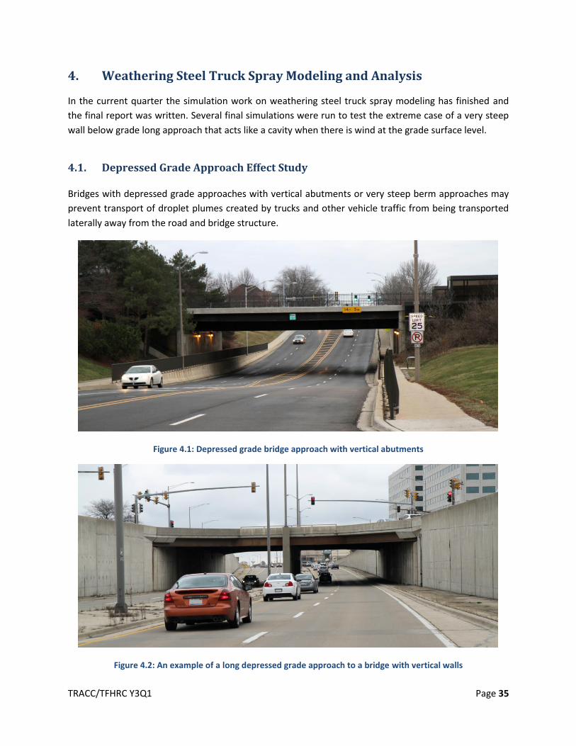
Bridges with depressed grade approaches with vertical abutments or very steep berm approaches may

prevent transport of droplet plumes created by trucks and other vehicle traffic from being transported

laterally away from the road and bridge structure.

Figure 4.1: Depressed grade bridge approach with vertical abutments

Figure 4.2: An example of a long depressed grade approach to a bridge with vertical walls


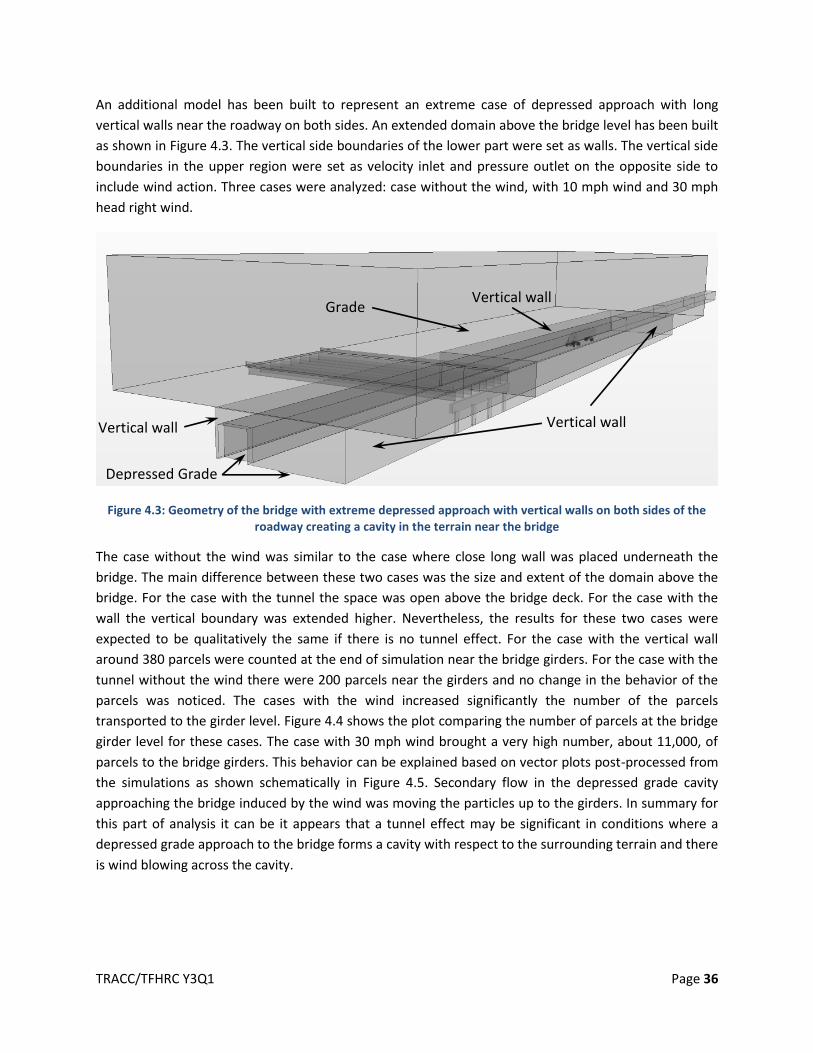
An additional model has been built to represent an extreme case of depressed approach with long

vertical walls near the roadway on both sides. An extended domain above the bridge level has been built

as shown in Figure 4.3. The vertical side boundaries of the lower part were set as walls. The vertical side

boundaries in the upper region were set as velocity inlet and pressure outlet on the opposite side to

include wind action. Three cases were analyzed: case without the wind, with 10 mph wind and 30 mph

head right wind.

Figure 4.3: Geometry of the bridge with extreme depressed approach with vertical walls on both sides of the roadway creating a cavity in the terrain near the bridge

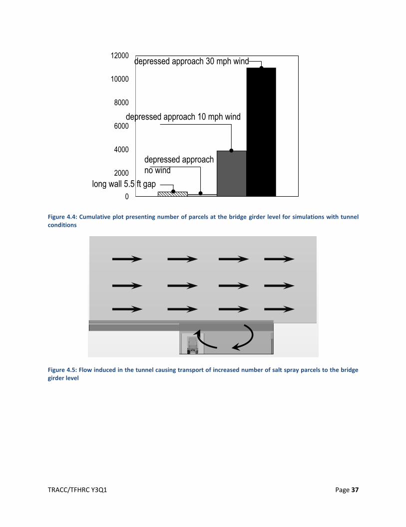
The case without the wind was similar to the case where close long wall was placed underneath the

bridge. The main difference between these two cases was the size and extent of the domain above the

bridge. For the case with the tunnel the space was open above the bridge deck. For the case with the

wall the vertical boundary was extended higher. Nevertheless, the results for these two cases were

expected to be qualitatively the same if there is no tunnel effect. For the case with the vertical wall

around 380 parcels were counted at the end of simulation near the bridge girders. For the case with the

tunnel without the wind there were 200 parcels near the girders and no change in the behavior of the

parcels was noticed. The cases with the wind increased significantly the number of the parcels

transported to the girder level. Figure 4.4 shows the plot comparing the number of parcels at the bridge

girder level for these cases. The case with 30 mph wind brought a very high number, about 11,000, of

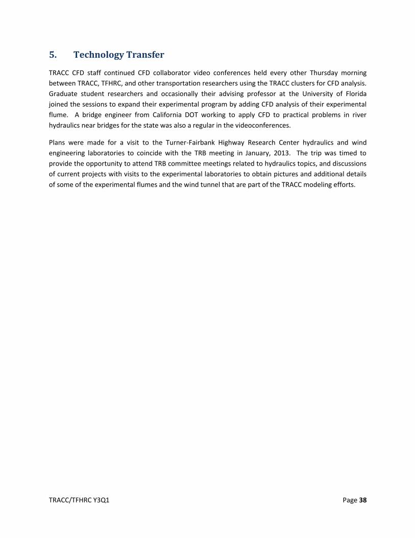
parcels to the bridge girders. This behavior can be explained based on vector plots post-processed from

the simulations as shown schematically in Figure 4.5. Secondary flow in the depressed grade cavity

approaching the bridge induced by the wind was moving the particles up to the girders. In summary for

this part of analysis it can be it appears that a tunnel effect may be significant in conditions where a

depressed grade approach to the bridge forms a cavity with respect to the surrounding terrain and there

is wind blowing across the cavity.

Vertical wall Vertical wall

Grade Vertical wall

Depressed Grade


Figure 4.4: Cumulative plot presenting number of parcels at the bridge girder level for simulations with tunnel conditions

Figure 4.5: Flow induced in the tunnel causing transport of increased number of salt spray parcels to the bridge girder level

0

2000

4000

6000

8000

10000

12000

long wall 5.5 ft gap

depressed approach no wind

depressed approach 10 mph wind

depressed approach 30 mph wind


5. Technology Transfer

TRACC CFD staff continued CFD collaborator video conferences held every other Thursday morning

between TRACC, TFHRC, and other transportation researchers using the TRACC clusters for CFD analysis.

Graduate student researchers and occasionally their advising professor at the University of Florida

joined the sessions to expand their experimental program by adding CFD analysis of their experimental

flume. A bridge engineer from California DOT working to apply CFD to practical problems in river

hydraulics near bridges for the state was also a regular in the videoconferences.

Plans were made for a visit to the Turner-Fairbank Highway Research Center hydraulics and wind

engineering laboratories to coincide with the TRB meeting in January, 2013. The trip was timed to

provide the opportunity to attend TRB committee meetings related to hydraulics topics, and discussions

of current projects with visits to the experimental laboratories to obtain pictures and additional details

of some of the experimental flumes and the wind tunnel that are part of the TRACC modeling efforts.


6. TRACC Facility and User Support for TFHRC

The new Zephyr cluster is now in production mode and TRACC users in the CFD and CSM application

areas are being encouraged to use it. The TRACC Wiki has been updated to include changes needed for

users to run on either of the TRACC clusters. The application notes for STAR-CCM+ and the LS-DYNA

related software have been updated to include information for the new Zephyr cluster.

Energy Systems Division Argonne National Laboratory 9700 South Cass Avenue, Bldg. 362 Argonne, IL 60439-4815 www.anl.gov Argonne National Laboratory is a U.S. Department of Energy laboratory managed by UChicago Argonne, LLC

http://www.anl.gov/

Documents

Computational Mechanics Research and Support for ... · Computational Mechanics Research and Support for Aerodynamics and Hydraulics at TFHRC, Year 3 Quarter 1 Progress Report by