Embed Size (px)
Citation preview
Computational Models and Complexities of Tarski’s
Fixed Points∗
Chuangyin DangDept. of Systems Engineering & Engineering Management
City University of Hong KongKowloon, Hong Kong
E-Mail: [email protected]
Qi QiDept. of Management Science & Engineering
Stanford UniversityStanford, CA 94305-4026
E-Mail: [email protected]
Yinyu YeDept. of Management Science & Engineering
Stanford UniversityStanford, CA 94305-4026
E-Mail: [email protected]
Abstract
We consider two models of computation for Tarski’s order preserving function f related to fixedpoints in a complete lattice: the oracle function model and the polynomial function model. Wedevelop a complete understanding under the oracle function model for finding a Tarski’s fixed pointas well as determining the uniqueness of Tarski’s fixed point in both the lexicographic orderingand the componentwise ordering lattices. Moreover, we present a polynomial-time reduction ofan integer program to an order preserving mapping f from a lattice L into itself. As a result ofthis reduction, we prove that, when f is given as a polynomial function, determining whether ornot f has a unique fixed point is Co-NP hard.
Keywords: Lexicographic Ordering, Componentwise Ordering, Lattice, Finite Lattice, OrderPreserving Mapping, Fixed Point, Integer Programming, Co-NP Completeness, Co-NP Hardness
1 Introduction
A partially order set L is defined with ¹ as a binary relation on the set L such that ¹ is reflexive,transitive, and anti-symmetric. A lattice is a partially ordered set (L,¹), in which any two elements
∗This work was partially supported by GRF: CityU 113308 of the Government of Hong Kong SAR.
x and y have a least upper bound (supremum), supL(x,y) = infz ∈ L | x ¹ z and y ¹ z, and agreatest lower bound (infimum), infL(x,y) = supz ∈ L | z ¹ x and z ¹ y, in the set. A lattice(L,¹) is complete if every nonempty subset of L has a supremum and an infimum in L. Let f be amapping from L to itself. f is order-preserving if f(x) ¹ f(y) for any x and y of L with x ¹ y.
The well-known Tarski’s fixed point theorem (Tarski)[23] asserts that, if (L,¹) is a completelattice and f is order-preserving from L into itself, then there exists some x∗ ∈ L such that f(x∗) =x∗. This theorem plays a crucial role in the study of supermodular games (or games with strategiccomplementarities) for economic analysis. Supermodular games were formalized in Topkis [24] andhave been extensively applied in the literature such as Bernstein and Federgruen [2][3], Cachon [6],Cachon and Lariviere [7], Fudenberg and Tirole [15], Lippman and McCardle [19], Milgrom andRoberts [20][21], Milgrom and Shannon [22], Topkis [25], and Vives [26][27]. To compute a Nashequilibrium of a supermodular game, a generic approach is to convert it into the computation of afixed point of an order preserving mapping. Recently, an algorithm has been proposed in Echenique[14] to find all pure strategy Nash equilibria of a supermodular game, which motivated to the studyin this paper.
An efficient computational algorithm for the fixed point has been a recognized important technicaladvantage in applications. Further, it is sometimes desirable to know if an already-found fixed pointfor such applications is unique or not, for the decision whether additional resource should be spentto improve the already found solution. There were some interesting complexity results in algorithmicgame theory research along this line, on determining whether or not a game has a unique equilibriumpoint. For the bimatrix game, Gilboa and Zemel [16] showed that it is NP-hard to determine whetheror not there is a second Nash equilibrium. For this problem, computing even one equilibrium (whichis know to exist), is already difficult and no polynomial time algorithms are known: Nash equilibriumfor the bimatrix game is known to be PPAD-complete [11]. Similar cases are known for other problemssuch as the market equilibrium computation (Codenotti et al.)[5].
In this work, we consider the fixed point computation of order preserving functions over a completelattice, both for finding a solution and for determining the uniqueness of an already-found solution.We are interested in both the oracle function model and polynomial function model. For the fixedpoint problem, the domain space is usually huge. As we are considering a discrete version with thelattice, the search space is well-defined. For an instance of the problem, we would need an orderpreserving function and functions for lattice operations. For those functions, one or two latticepoints are given as the input and another lattice point will be returned as the output. Therefore, themost succinct representation of the lattice (L,¹) will be those enough to represent a lattice pointwhich requires O(log |L|) bits. That observation has been the main motivation in most interestingdiscussions restricting the input size to log |L|. It is enough for the representation of a variable in alattice of size |L|. Both the oracle function model and the polynomial time function model returnthe function value f(x) on a lattice node x where x is of size log |L|. They differ in the ways thefunctions are computed. The polynomial time function model computes f(x) by an explicitly givenalgorithm, in time polynomial of log |L|. The oracle model, on the other hand, always returns thevalue in one oracle step. More details on comparing the two models can be found in Section 2.2.
1.1 Main Results
We focus on the componentwise ordering and lexicographic ordering finite lattices. Let Ld = x ∈Zd | a ≤ x ≤ b, where a and b are two finite vectors of Zd with a < b. We denote the compo-
2
nentwise ordering and the lexicographic ordering as ≤c and ≤l, respectively. Clearly, (Ld,≤c) is afinite lattice with the componentwise ordering and (Ld,≤l) is a finite lattice with the lexicographicordering.
Let fc and fl be an order preserving mapping from Ld into itself under the componentwiseordering and the lexicographic ordering, respectively.
1.1.1 Oracle Function Model
When fl(·) and fc(·) are given as oracle functions, we develop a complete understanding for findinga Tarski’s fixed point as well as determining the uniqueness of Tarski’s fixed point in both thelexicographic ordering and the componentwise ordering lattices.
We develop an algorithm of time complexity O((log |L|)d) to find a Tarski’s fixed point on thecomponentwise ordering lattice (L,≤c), for any dimension d. This algorithm is based on the binarysearch method. We first present the algorithm when d = 2. Following a similar principle, thisalgorithm can be generalized to any constant dimension. This is the first known polynomial timealgorithm for finding a Tarski’s fixed point in terms of the componentwise ordering. In the literatures,a polynomial time algorithm was only known for the total order lattices (Chang et al.) [8], whereany pair of lattice points are comparable.
On the other hand, given a general lattice (L,¹) with one already known fixed point, to find outwhether it is unique will take Ω(|L|) time for any algorithm. For a componentwise ordering lattice,we derive a Θ(N1 + N2 + · · ·+ Nd) matching bound for determining the uniqueness of Tarski’s fixedpoint, where L = x ∈ Zd | a ≤ x ≤ b and Ni = bi−ai. In addition, we prove this matching boundfor both deterministic algorithm and randomized algorithm.
For a lexicographic ordering lattice, it can be viewed as a componentwise ordering lattice withdimension one by an appropriate polynomial time transformation to change the oracle function forthe d-dimension space to an oracle function on the 1-dimension space. All the above results can betransplanted onto the lexicographic ordering lattice with a set of related parameters.
1.1.2 Polynomial Function Model
Under the polynomial time function model, our polynomial time algorithm applies when the dimen-sion is any finite constant. When the dimension is used as a part of the input size in unary, we firstpresent a polynomial-time reduction of integer programming to an order preserving mapping f froma componentwise ordering lattice L into itself. As a result of this reduction, we obtain that, given fas a polynomial time function, determining whether f has a unique fixed point in L is a Co-NP hardproblem. Furthermore, even when the dimension is one, we also find a polynomial-time reductionof determining the feasibility of an integer programming to the uniqueness of Tarski’s fixed pointin a lexicographic lattice. This shows that determining the uniqueness of Tarski’s fixed point in alexicographic lattice is Co-NP hard though there exists a polynomial-time algorithm for computinga Tarski’s fixed point in a lexicographic lattice in any dimension.
1.2 Related Work
For the oracle function model, when the lattice (L,¹) has a total order, i.e., all the point in thelattice is comparable, there is a matching bound of θ(log |L|) in Chang et al.[8]. It is a special case of
3
our result for the oracle function model since a total order lattice is equivalent to a componentwiseordering lattice of dimension one.
1.3 Organization
The rest of the paper is organized as follows. First, in Section 2, we present definitions as well as thedifference of the polynomial function model and the oracle function model. We develop polynomialtime algorithms in oracle function model for componentwise ordering and lexicographic ordering inSection 3. In Section 4, we derive the matching bound for determining the uniqueness of Tarski’s fixedpoint under the oracle function model. We prove co-NP hardness for determining the uniqueness ofTarski’s fixed point under the polynomial function model in Section 5. We conclude with discussionand remarks on our results and open problems in Section 6.
2 Preliminaries
In this section, we first introduce formal definitions of some relevant concepts as well as Tarski’sfixed point theorem. We then compare the difference between the oracle function model and thepolynomial function model.
2.1 Definitions and Theorems
Definition 1. (Partial Order vs. Total Order) A relationship ¹ on a set L is a partial order if itsatisfies reflexivity (∀a ∈ L : a ¹ a); antisymmetry (a ¹ b and b ¹ a implies a = b); transitivity(a ¹ b and b ¹ c implies a ¹ c). It is a total order if ∀a,b ∈ L: either a ¹ b or b ¹ a.
Definition 2. (Lattice) (L,¹) is a lattice if
1. L is a partial ordered set;
2. There are two operations: meet ∧ and join ∨ on any pair of elements a,b of L such thata,b ¹ a ∨ b and a ∧ b ¹ a,b
The lattice is complete if, for any subset A = a1,a2, · · · ,ak ⊆ L, there is a unique meet and aunique join:
∧A = (a1 ∧ a2 ∧ · · · ∧ ak) and
∨A = (a1 ∨ a2 ∨ · · · ∨ ak).
For simplicity, we use L for a lattice when no ambiguity exists on ¹. We should specify ¹whenever it is necessary.
Definition 3. (Order Preserving Function) A function f on a lattice (L,¹) is order preserving ifa ¹ b implies f(a) ¹ f(b).
Theorem 1. (Tarski’s Fixed Point Theorem)[23]. If L is a complete lattice and f an increasingfrom L to itself, there exists some x∗ ∈ L such that f(x∗) = x∗, which is a fixed point of f .
This theorem guarantees the existence of fixed points of any order-preserving function f : L → Lon any nonempty complete lattice.
Definition 4. (Lexicographic Ordering Function). Given a set of points on a d-dimensional spaceRd, the lexicographic ordering function ≤l is defined as:
∀x,y ∈ Rd, x ≤l y if either x = y or xi = yi, i = 1, 2, . . . , k − 1, and xk < yk for some k ≤ d.
4
Definition 5. (Componentwise Ordering Function). Given a set of points on a d-dimensional space,the componentwise ordering function ≤c is defined as:
∀x,y ∈ Rd, x ≤c y if ∀i ∈ 1, 2, · · · , d : xi ≤ yi.
2.2 The oracle function model versus the polynomial time function model.
In recent years, the computational complexities of the fixed point computation has received intensiveexaminations, under both the oracle function model and the polynomial time function model.
The differences of these two models have an impact on the computational complexities of them.For the oracle function model, the function value f(x) is revealed only if the value x is specifiedto the oracle. The oracle is restricted to be consistent in that the answer has to be consistent inthe returned values, i.e., the returned values of the same input x in different queries must be thesame. However, it still has the flexibility in the choices of function values dependent on the algorithmdesigned to find the guaranteed fixed point. In this sense, the oracle has a huge range of functions tochoose from, and hence makes it difficult for an algorithm to deal with all the answer sequences withrespect to its query sequences. The oracle model allows for any function to be used and thereforeoften demands a large complexity to handle every case. The polynomial time function model, on theother hand, provides, a prior, a function computable in polynomial time with respect to the inputsize, such as a circuit of AND/OR/NOT gates of size polynomial in the input size. It is possible thatthe algorithmic designer could utilize the knowledge of the polynomial time computable functionto design a fast fixed point computation procedure though there has no universal framework to tellus how to do it. Therefore, the polynomial time function model can only accommodate a muchless number of functions than the oracle function model. Hence, one may only need to consider asmaller set of functions than that in the oracle function model. Hence, the oracle function modeloften demands a large computational complexity. More details on comparing these two models inthe general fixed point computation can be found in (Deng et al.)[13].
3 Polynomial Time Algorithm under Oracle Function Model
In this section, we consider the complexity of finding a Tarski’s fixed point in any constant dimensiond with the function value f given by an oracle. Chang et al. [8] proved that a fixed point can befound in time polynomial when the given lattice is total order.
Define L = x ∈ Zd | a ≤ x ≤ b, where a and b are two finite vectors of Zd with a < b.
Theorem 2. (Chang et al.)[8] When (L,¹) is given as input and the order preserving function f isgiven as oracles, a Tarski’s fixed point can be found in time O(log |L|) on a finite lattice when ¹ isa total order on L.
Since any two vectors in the lexicographic ordering is comparable, the lexicographic ordering isa total order. We have
Corollary 1. When (L,¹) is given as input and the order preserving function f is given as oracles,a Tarski’s fixed point can be found in time O(log |L|) on a finite lattice when ¹ is the lexicographicordering on L.
The proof is rather standard utilizing the total order property of the lexicographic ordering.As the componentwise ordering lattice cannot be modeled as a total order, it leaves open the oracle
5
complexity of finding a fixed point in componentwise ordering lattice. Here we show that this problemis also polynomial time solvable, by designing a polynomial algorithm to find a fixed point of f intime O((log |L|)d) given componentwise ordering lattice L.
The algorithm exploits the order properties of the componentwise lattice and applying the binarysearch method with a dimension reduction technique. To illustrate the main ideas, we first considerthe 2D case before moving on to the general case.
Without loss of generality (WLOG), we assume L is an N × N square centered at point (0, 0).The componentwise ordering is denoted as ≤c.
Algorithm 3.1. Point check() (A polynomial algorithm for 2D lattice)
• Input:
2-dimensional lattice (L,≤c), |L| = N2 (Input size to the oracle is 2 log N since the input sizefor both dimensions to the oracle is log N . )
Oracle function f . f is an order preserving function. ∀x ∈ L, f(x) ∈ L and f(x) ≤c f(y) ifx ≤c y, ∀x,y ∈ L
• Point check(L, f)
Let x0 be the center point in L. Let xL be the left most point in L such that xL2 = x0
2. Let xR
be the right most point in L such that xR2 = x0
2.
1. If f(x0) = x0,return(x0);end;2. If f(x0) ≥c x0,L′ = x|x ≥c x0,x ∈ L. Point check(L′, f);3. If f(x0) ≤c x0, L′′ = x|x ≤c x0,x ∈ L. Point check(L′′, f);4. If f(x0)1 < x0
1 and f(x0)2 > x02, Binary Search(xL,x0);
5. If f(x0)1 > x01 and f(x0)2 < x0
2, Binary Search(x0,xR);
• Binary Search(x,y)
Let xm = b1/2(x + y)c1. If f(xm) = xm,return(xm);end;2. If f(xm) ≥c xm, L′ = x|x ≥c xm,x ∈ L. Point check(L′, f);3. If f(xm) ≤c xm, L′′ = x|x ≤c xm,x ∈ L. Point check(L′′, f);4. If f(xm)1 < xm
1 and f(xm)2 > xm2 , Binary Search(x,xm);
5. If f(xm)1 > xm1 and f(xm)2 < xm
2 , Binary Search(xm,y);
Theorem 3. When the order preserving function f is given as an oracle, a Tarski’s fixed point canbe found in time O(log2 N) on a finite 2D lattice formed by integer points of a box with side lengthN by using Algorithm 3.1 Point check.
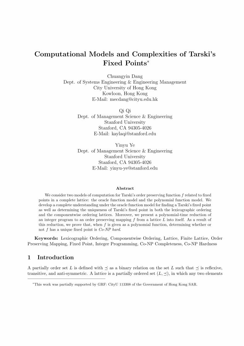
Proof. Start from a lattice of size |L|, we first prove that in at most O(log N) steps the abovealgorithm either finds the fixed point or reduces the input lattice to size |L|/2.
6
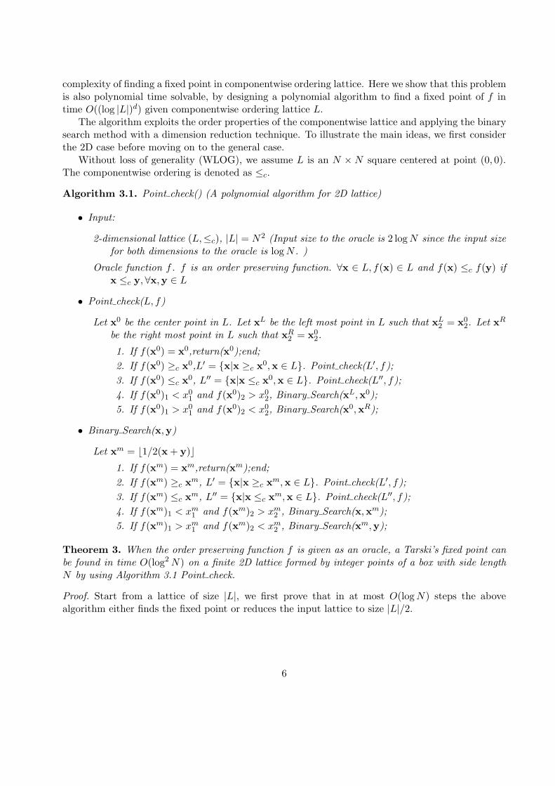
(a) Point check() (b) Binary Search()
Figure 1: A polynomial algorithm for 2D Lattice
Consider the algorithm Point check(L, f).
1. Case I: If f(x0) = x0, x0 is the fixed point which is found in 1 step.
2. Case II: If f(x0) ≥c x0, since f is an order preserving function, ∀y ≥c x0, we have f(y) ≥c
f(x0) ≥c x0. Let L′ = x|x ≥c x0,x ∈ L. Define f ′(x) = f(x), ∀x ∈ L′. Then f ′ : L′ → L′ isa order preserving function on the complete lattice L′. By Tarski’s fixed point theorem, theremust exist a fixed point in L′. Next we only need to check L′ which is only 1/4 size of |L|.
3. Case III: If f(x0) ≤c x0, similar to the analysis in Case II, we only need to consider L′′ =x|x ≤c x0,x ∈ L which is only 1/4 size of |L| in the next step.
4. Case IV: If f(x0)1 < x01 and f(x0)2 > x0
2, we prove that Binary Search(xL,x0) finds a fixedpoint or reduce the size of the lattice by half in log N
2 steps. Since f is an order preservingfunction, ∀ adjacent points u ≤c v ∈ L (i.e., ||u − v||∞ = 1), it is impossible that f(u)1 > u1
and f(v)1 < v1. Thus, on a line segment [x,y] where x2 = y2, if f(x)1 ≥ x1 and f(y)1 < y1,there must exist a point z such that f(z)1 = z1. On the other hand, we have f(x0)1 < x0
1
and by the boundary condition f(xL)1 ≥ xL1 , therefore, there must exist a point x′ ∈ [xL, x0)
such that f(x′)1 = x′1. This point x′ can be found in time log N2 by using binary search. If
f(x′)2 > x′2, similar to the analysis in Case II, we only need to consider L′ = x|x ≥c x′,x ∈ Lwhich is at most 1/2 size of |L| in the next step. If f(x′)2 < x′2, we only need to considerL′′ = x|x ≤c x′,x ∈ L which is at most 1/4 size of |L| in the next step. If f(x′)2 = x′2, thenx′ is the fixed point.
5. Case V: If f(x0)1 > x01 and f(x0)2 < x0
2, similarly, we can prove that Binary Search(x0,xR)findsa fixed point or reduce the size of the lattice by half in log N
2 steps.
7
The size of the lattice is reduced by half in every O(log N) steps. Therefore, the algorithm findsa fixed point in at most O(log N × log L) = O(log2 N) steps.
The above algorithm can be generalized to any constant dimensional lattice with L = x ∈Zd | a ≤ x ≤ b, where a and b are two finite vectors of Zd with a < b. We reduce a (d + 1)-dimension problem to a d-dimension one. Assume we have an algorithm for a d-dimensional problemwith time complexity O(logd |L|). Let the algorithm be Ad(L, f).
Consider a d+1-dimensional lattice (L,≤c). Choose the central point in L, and denote it by O =(O1, O2, · · · , Od+1)T . Take the section of L by a hyperplane parallel to xd+1 = 0 passing through O.Denote it as Ld. Clearly, it is a d-dimensional lattice. We define a new oracle function fd on Ld, basedon the oracle function f on L. Define fd(x1, x2, · · · , xd) = (y1, y2, · · · , yd), if f(x1, x2, · · · , xd, Od+1) =(y1, y2, · · · , yd, yd+1). We apply the algorithm Ad(Ld, fd) to obtain a Tarski’s fixed point in time(log |L|)d. Let the fixed point be denoted by x∗. Therefore, f(x∗) = (x∗, Od+1) + aed+1 or f(x∗) =(x∗, Od+1)− aed+1, where a is some constant, ed+1 is a d + 1 dimensional unit vector with 1 on itsd + 1th position.
In either case, we obtain a new box B with size no more than half of the original box definedby [a,b], such that f(·) maps all points in B into B and is order preserving. We can apply thealgorithm recursively on B. The base case can be handled easily. Therefore the total time is
T (|L|d+1) ≤ T (|L|d+1
2) + O(logd |L|).
It follows that T (|L|d+1) = O(logd |L|).Algorithm 3.2. Fixed point() (A polynomial algorithm for any constant dimensional lattice)
• Input:
d dimensional lattice Ld, WLOG, |Ld| = Nd (Input size to the oracle is d log N since the inputsize for both dimensions to the oracle is log N . )
Oracle function fd. fd is an order preserving function. ∀x ∈ Ld, fd(x) ∈ Ld and fd(x) ≤c
fd(y) if x ≤c y, ∀x,y ∈ Ld
• Fixed point(Ld)
1. If d > 1
(a) Let x0 be the center point in Ld.(b) Let Ld−1 = x = (x1, x2, · · · , xd−1)|(x, x0
d) ∈ Ld.(c) Let fd−1(x) = (fd(x, x0
d)1, fd(x, x0
d)2, · · · , fd(x, x0d)d−1).
(d) x∗ =Fixed point(Ld−1).(e) If fd(x∗, x0
d)d > x0d, Ld = x|x ≥ (x∗, x0
d); Fixed point(Ld);(f) If fd(x∗, x0
d)d < x0d, Ld = x|x ≤ (x∗, x0
d); Fixed point(Ld);(g) If fd(x∗, x0
d)d = x0d, return (x∗, x0
d); end;
2. If d = 1, let xL be the left end point and xR be the right end point. binary search(xL,xR, fd).
• binary search(x,y, f)
8
1. If f(xL) = 0, output xL;
2. else if f(xR) = 0, output xR;
3. else
(a) If f(b1/2(xL + xR)c) < b1/2(xL + xR)c, binary search(xL, b1/2(xL + xR)c, f);(b) If f(b1/2(xL + xR)c) > b1/2(xL + xR)c, binary search(b1/2(xL + xR)c,xR, f);(c) else output x∗.
Theorem 4. When the order preserving function f is given as an oracle, a Tarski’s fixed point canbe found in time O(logd |L|) on a componentwise ordering lattice (L,≤c).
4 Determining the Uniqueness under Oracle Function Model
It has been a natural question to check whether there is another fixed point after finding the firstone, such as in the applications for finding a Nash equilibrium (Echenique)[14] . In this section wedevelop a lower bound that, given a general lattice L with one already known fixed point, determiningwhether it is unique will take Ω(|L|) time for any algorithm. Even for the componentwise orderinglattice, we also derive a Θ(N1 + N2 + · · · + Nd) matching bound for determining the uniqueness offixed points even for randomized algorithms. The technique builds on and further reveals crucialproperties of mathematical structures for fixed points.
Theorem 5. Given a lattice (L,¹), an order preserving function f and a fixed point x0, it takestime Ω(|L|) for any deterministic algorithm to decide whether there is a unique fixed point.
Proof. Consider the lattice on a real line: 0 ≺ 1 ≺ 2 ≺ · · · ≺ L− 1. Let x0 = 0, define f(0) = 0 andf(x) = x−1 for all x ≥ 1 except a possible fixed point x∗. f(x∗) = x∗ or f(x∗) = x∗−1 which is notknown until we query x∗. Given a deterministic algorithm A, define yj be the j-th item A queriedin its effort to find x∗. Our adversary will answer x− 1 whenever A asks for f(x) until the last itemwhen the adversary answers x. Clearly this derives a lower bound of L.
For a randomized algorithm R, let pij be the probability R queries x = i on its j-th query. Letk be the total number of queries R makes. We have:
k∑
j=1
|L|−1∑
i=0
pij = k.
Therefore, there exists i∗ such thatk∑
j=1
pi∗j ≤ k
|L| .
The adversary will place f(i∗) = i∗, which is queried with probability k|L| < 1/2 when we choose
k = |L|−12 . Therefore, we have
Theorem 6. Given a lattice (L,¹), an order preserving function f and a fixed point x0, it takes timeΩ(|L|) for any randomized algorithm to decide whether there is a unique fixed point with probabilityat least 1/2.
9
As we noted before, for a lexicographic ordering lattice, it can be viewed as a total orderinglattice or componentwise ordering lattice with dimension one by an appropriate polynomial timetransformation to change the oracle function for the d-dimension space to an oracle function on the1-dimension space. Therefore,
Corollary 2. Given a lattice (L,≤l), an order preserving function f and a fixed point x0, it takestime Ω(|L|) both for any deterministic algorithm and for any randomized algorithm to decide whetherthere is a unique fixed point with probability at least 1/2.
Next we consider a componentwise ordering lattice.
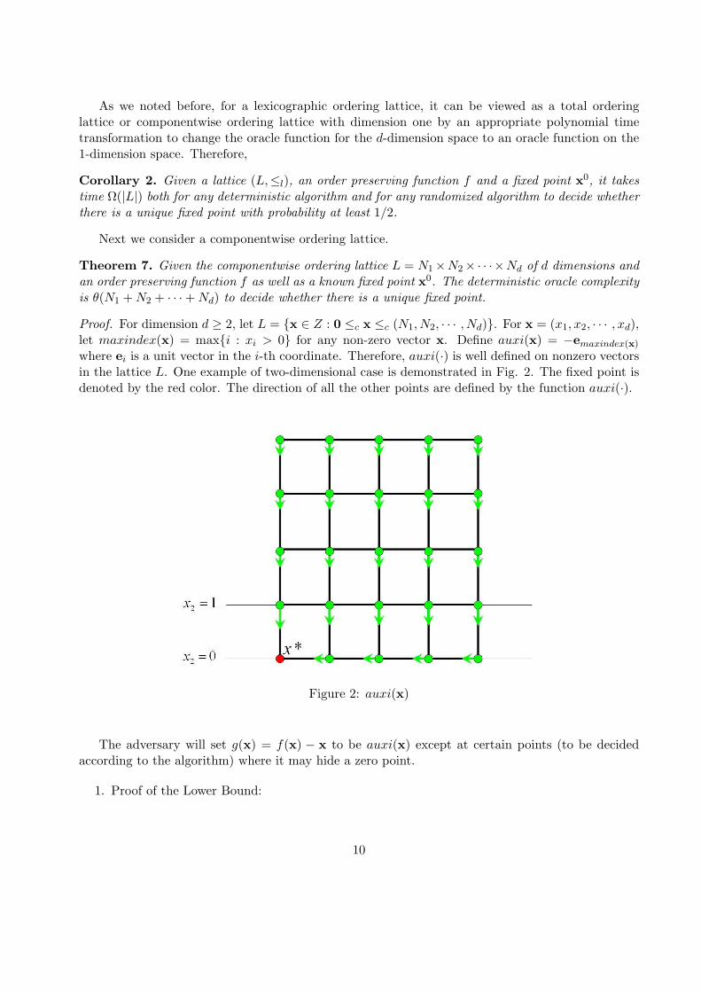
Theorem 7. Given the componentwise ordering lattice L = N1×N2×· · ·×Nd of d dimensions andan order preserving function f as well as a known fixed point x0. The deterministic oracle complexityis θ(N1 + N2 + · · ·+ Nd) to decide whether there is a unique fixed point.
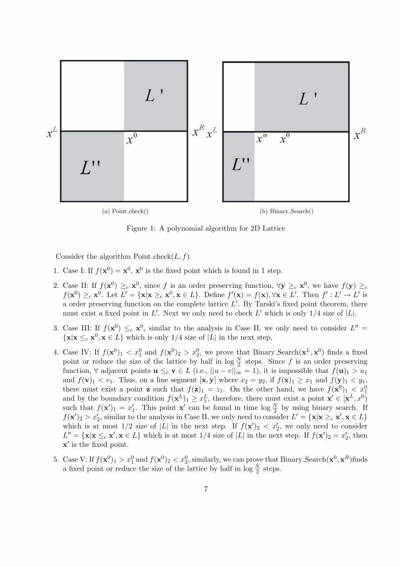
Proof. For dimension d ≥ 2, let L = x ∈ Z : 0 ≤c x ≤c (N1, N2, · · · , Nd). For x = (x1, x2, · · · , xd),let maxindex(x) = maxi : xi > 0 for any non-zero vector x. Define auxi(x) = −emaxindex(x)
where ei is a unit vector in the i-th coordinate. Therefore, auxi(·) is well defined on nonzero vectorsin the lattice L. One example of two-dimensional case is demonstrated in Fig. 2. The fixed point isdenoted by the red color. The direction of all the other points are defined by the function auxi(·).
Figure 2: auxi(x)
The adversary will set g(x) = f(x) − x to be auxi(x) except at certain points (to be decidedaccording to the algorithm) where it may hide a zero point.
1. Proof of the Lower Bound:
10
First consider x such that xd = 0. It constitutes a solution of d− 1 dimensions. By inductivehypothesis, it requires time N1 + N2 + · · · + Nd−1 to decide whether or not there is one zeropoint at xd = 0.
Second, when there is no such zero point, we need to decide if there is a zero point at x withxd > 0. Fixing any i > 0, we will set, for all x with xd = i, g(x) = 0 whenever none of such xis queried, and set g(x) = −ei otherwise. This will take Nd queries.
One may note that the adversary always answers a non-zero value. In fact, for any pairi = maxindex(x) and j = xi not queried, the adversary can make g(x) = 0 without violatingthe order preserving property.
2. Proof of the Upper Bound:
We design an algorithm which always queries the componentwise maximum point of the latticexmax = (N1, N2, · · · , Nd). We should have g(xmax) ≤c 0. We are done if it is zero. Otherwise,there must exist some i, such that g(xmax)i < 0. The problem is reduced to a smaller latticeL′ = x ∈ Z : 0 ≤c x ≤c (N1, N2, · · · , Ni−1, Ni − 1, Ni+1, · · · , Nd) which has a total sum ofside lengths at most N1 + N2 + · · ·+ Nd − 1. The claim follows.
For the randomized lower bound, it follows in the same way as in the one-dimensional case for ageneral lattice. We can always set f(x) = 0 for all x with i = maxindex(x) and j = xi if none ofsuch x is queried.
Corollary 3. Given the componentwise ordering lattice L = N1×N2×· · ·×Nd of d dimensions andan order preserving function f as well as a known fixed point x0. It takes time θ(N1 +N2 + · · ·+Nd)for any randomized algorithm to decide whether there is a unique fixed point with probability at least1/2.
5 Determining Uniqueness under Polynomial Function Model
In this section, we consider the dimension as a part of the input size in unary and develop a hardnessproof for the polynomial function model for determining the uniqueness of a given fixed point. Westart with a polynomial-time reduction from a special class of integer programming which is NP-complete to one of finding a second Tarski’s fixed point, by deriving an order preserving mapping ffrom a componentwise ordering lattice L into itself, with a given fixed point. Therefore, given f as apolynomial time function with a known fixed point, determining whether f has another fixed pointin L is an NP-hard problem. In other words, determining the uniqueness of a Tarski’s fixed point isco-NP-hard.
Furthermore, even for the case when the dimension is one, the uniqueness problem is still co-NP-hard. This can be done by designing a polynomial-time reduction of determining the feasibility ofan integer programming to the uniqueness of Tarski’s fixed point in a lexicographic lattice. As thelexicographic order defines a total order, it can be reduced to a one dimensional problem by findinga polynomial time algorithm for the order function calculation. It then follows that determiningthe uniqueness of Tarski’s fixed point in a lexicographic lattice is Co-NP hard though there exists
11
a polynomial-time algorithm for finding one Tarski’s fixed point in a lexicographic lattice in anydimension.
Let P = x ∈ Rn | Ax ≤ b be a full-dimensional polytope, where A is an m×n rational matrixsatisfying that each row of A has at most one positive entry and b a rational vector of Rm. It hasbeen shown in (Lagarias)[18] that
Theorem 8. [18] Determining whether there is an integer point in P is an NP-complete problem.
5.1 Co-NP-hard in Componentwise Ordering
Let N = 1, 2, . . . , n. For any real number α, let bαc denote the greatest integer less than or equal toα and dαe the smallest integer greater than or equal to α. For any vector x = (x1, x2, . . . , xn)> ∈ Rn,let bxc = (bx1c, bx2c, . . . , bxnc)> and dxe = (dx1e, dx2e, . . . , dxne)>. Given these notations, wepresent a polynomial-time reduction of integer programming, which is as follows.
For any x ∈ Rn, let P (x) = y ∈ P | y ≤c x. Then, as a direct result of the property of thematrix A, one can easily obtain that
Lemma 1. For any given x ∈ Rn, if x1 = (x11, x
12, . . . , x
1n)> ∈ P (x) and x2 = (x2
1, x22, . . . , x
2n)> ∈
P (x), then
x = max(x1,x2) = (maxx11, x
21,maxx1
2, x22, . . . , maxx1
n, x2n)> ∈ P (x).
Let e = (1, 1, . . . , 1)> ∈ Rn. For any given v ∈ Rn, if P (v) 6= ∅, Lemma 1 implies thatmaxx∈P (v) e>x has a unique solution, which we denote by xv = (xv
1 , xv2 , . . . , xv
n)>.
Lemma 2. x ≤c xv for all x ∈ P (v).
Proof. Suppose that there is a point x0 = (x01, x
02, . . . , x
0n)> ∈ P (v) with x0
k > xvk for some
k ∈ N . Then, Lemma 1 implies that
xv0 = (maxx01, x
v1,maxx0
2, xv2, . . . ,maxx0
n, xvn)> ∈ P (v).
Thus, e>x0v > e>xv = maxx∈P (v) e>x. A contradiction arises. This completes the proof.Let xmax = (xmax
1 , xmax2 , . . . , xmax
n )> be the unique solution of maxx∈P e>x and xmin = (xmin1 , xmin
2 ,. . . , xmin
n )> with xminj = minx∈P xj , j = 1, 2, . . . , n. Then, xmin ≤c x ≤c xmax for all x ∈ P . Let
D(P ) = x ∈ Zn | xl ≤c x ≤c xu,
where xu = bxmaxc and xl = bxminc. Thus, D(P ) contains all integer points in P . Without loss ofgenerality, we assume that xl <c xmin (Let xl
i = xmini − 1 if xl
i = xmini for some i ∈ N). Obviously,
the sizes of both xl and xu are bounded by polynomials of the sizes of the matrix A and the vectorb since xl and xu are obtained from the solutions of linear programs with rational data.
For x ∈ Rn, we define h(x) = bd(x)c with
d(x) =
xl if P (x) = ∅,argmaxy∈P (x)e
>y otherwise.
It follows from Lemma 2 that d(x) is well defined.
12
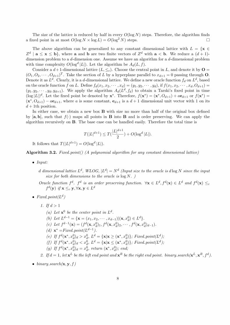
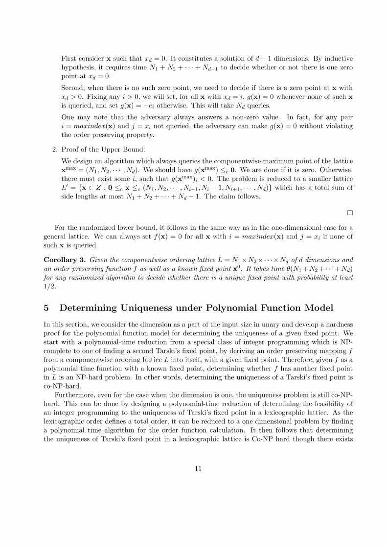
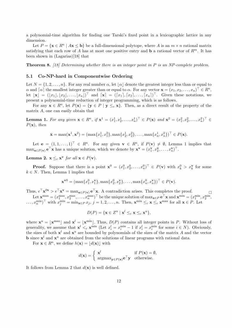
Example 1. Consider P = x ∈ R3 | Ax ≤c b, where
A =
2 −1 0−1 3 00 0 20 −1 −1
and b = (0,−10, 10, 0)>. For y = (−3,−4, 5)>, h(y) = (−3,−5, 5)>. An illustration of h can befound in Fig.3.
−5
−4
−3
−2
−5
−4.5
−43
3.5
4
4.5
5
h(y)
xu
xl
y
Figure 3: An Illustration of h
Lemma 3. h is an order preserving mapping from Rn to D(P ). Moreover, h(x∗) = x∗ 6= xl if andonly if x∗ is an integer point in P .
Proof. Let x1 and x2 be two different points of Rn with x1 ≤c x2. Then, P (x1) ⊆ P (x2). Thus,from the definition of d(x), we obtain that xmin ≤c d(x1) ≤c d(x2) ≤c xmax. The first part of thelemma follows immediately.
Let x∗ be an integer point in P . Then,
d(x∗) = argmaxy∈P (x∗)e>y = x∗.
Thus, h(x∗) = x∗ 6= xl.Let x∗ be a point in Rn satisfying that h(x∗) = x∗ 6= xl. Suppose that P (x∗) = ∅. Then,
d(x∗) = xl. Thus,x∗ = h(x∗) = bxlc = xl.
A contradiction occurs. Therefore, P (x∗) 6= ∅ and, consequently, d(x∗) ∈ P . Since
x∗ ≥c d(x∗) ≥c bd(x∗)c = h(x∗) = x∗,
13
hence, d(x∗) = bd(x∗)c = x∗. This completes the proof.Let (L,≤c) be a finite lattice and f an order preserving mapping from L into itself. As a corollary
of Theorem 8 and Lemma 3, we obtain that
Corollary 4. Given lattice (L,≤c) and an order preserving mapping f as a polynomial function,determining that f has a unique fixed point in L is a Co-NP hard problem.
It is a remark that the result can also be applied to derive a fixed-point iterative method fordetermining wether there is an integer point in such a polytope.
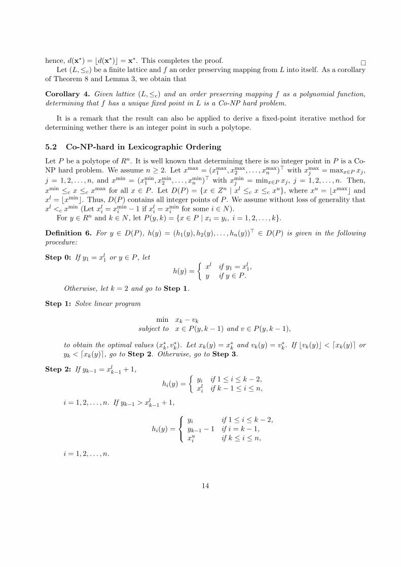
5.2 Co-NP-hard in Lexicographic Ordering
Let P be a polytope of Rn. It is well known that determining there is no integer point in P is a Co-NP hard problem. We assume n ≥ 2. Let xmax = (xmax
1 , xmax2 , . . . , xmax
n )> with xmaxj = maxx∈P xj ,
j = 1, 2, . . . , n, and xmin = (xmin1 , xmin
2 , . . . , xminn )> with xmin
j = minx∈P xj , j = 1, 2, . . . , n. Then,xmin ≤c x ≤c xmax for all x ∈ P . Let D(P ) = x ∈ Zn | xl ≤c x ≤c xu, where xu = bxmaxc andxl = bxminc. Thus, D(P ) contains all integer points of P . We assume without loss of generality thatxl <c xmin (Let xl
i = xmini − 1 if xl
i = xmini for some i ∈ N).
For y ∈ Rn and k ∈ N , let P (y, k) = x ∈ P | xi = yi, i = 1, 2, . . . , k.Definition 6. For y ∈ D(P ), h(y) = (h1(y), h2(y), . . . , hn(y))> ∈ D(P ) is given in the followingprocedure:
Step 0: If y1 = xl1 or y ∈ P , let
h(y) =
xl if y1 = xl1,
y if y ∈ P .
Otherwise, let k = 2 and go to Step 1.
Step 1: Solve linear program
min xk − vk
subject to x ∈ P (y, k − 1) and v ∈ P (y, k − 1),
to obtain the optimal values (x∗k, v∗k). Let xk(y) = x∗k and vk(y) = v∗k. If bvk(y)c < dxk(y)e or
yk < dxk(y)e, go to Step 2. Otherwise, go to Step 3.
Step 2: If yk−1 = xlk−1 + 1,
hi(y) =
yi if 1 ≤ i ≤ k − 2,xl
i if k − 1 ≤ i ≤ n,
i = 1, 2, . . . , n. If yk−1 > xlk−1 + 1,
hi(y) =
yi if 1 ≤ i ≤ k − 2,yk−1 − 1 if i = k − 1,xu
i if k ≤ i ≤ n,
i = 1, 2, . . . , n.
14
−1−0.5
00.5
1
−2
−1
0
1−2
−1.5
−1
−0.5
0
0.5 xu
h(y)
xl
y
Figure 4: An Illustration of h
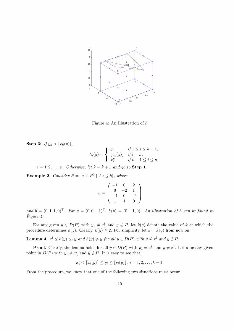
Step 3: If yk > bvk(y)c,
hi(y) =
yi if 1 ≤ i ≤ k − 1,bvk(y)c if i = k,xu
i if k + 1 ≤ i ≤ n,
i = 1, 2, . . . , n. Otherwise, let k = k + 1 and go to Step 1.
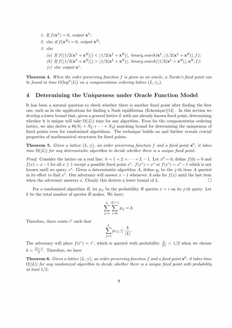
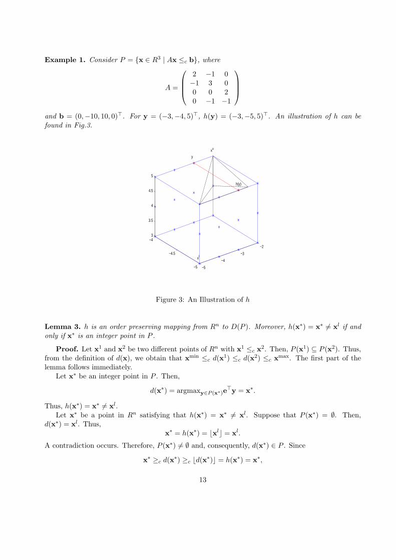
Example 2. Consider P = x ∈ R3 | Ax ≤ b, where
A =
−1 0 20 −2 1−1 0 −21 1 0
and b = (0, 1, 1, 0)>. For y = (0, 0,−1)>, h(y) = (0,−1, 0). An illustration of h can be found inFigure 4.
For any given y ∈ D(P ) with y1 6= xl1 and y /∈ P , let k(y) denote the value of k at which the
procedure determines h(y). Clearly, k(y) ≥ 2. For simplicity, let k = k(y) from now on.
Lemma 4. xl ≤ h(y) ≤l y and h(y) 6= y for all y ∈ D(P ) with y 6= xl and y /∈ P .
Proof. Clearly, the lemma holds for all y ∈ D(P ) with y1 = xl1 and y 6= xl. Let y be any given
point in D(P ) with y1 6= xl1 and y /∈ P . It is easy to see that
xli < dxi(y)e ≤ yi ≤ bvi(y)c, i = 1, 2, . . . , k − 1.
From the procedure, we know that one of the following two situations must occur.
15
Situation 1: Consider that bvk(y)c < dxk(y)e or yk < dxk(y)e.1. Suppose that yk−1 = xl
k−1 + 1. Then, from Step 2, we find that
hi(y) =
yi if 1 ≤ i ≤ k − 2,xl
i if k − 1 ≤ i ≤ n,
i = 1, 2, . . . , n. Thus, it follows from yk−1 > xlk−1 that xl ≤ h(y) ≤ y and h(y) 6= y.
2. Suppose that yk−1 > xlk−1 + 1. Then, from Step 2, we find that
hi(y) =
yi if 1 ≤ i ≤ k − 2,yk−1 − 1 if i = k − 1,xu
i if k ≤ i ≤ n,
i = 1, 2, . . . , n. Thus, it follows from yk−1 − 1 < yk−1 that xl ≤ h(y) ≤l y and h(y) 6= y.
Situation 2: Consider that bvk(y)c ≥ dxk(y)e and yk > bvk(y)c. From Step 3, we find that
hi(y) =
yi if 1 ≤ i ≤ k − 1,bvk(y)c if i = k,xu
i if k + 1 ≤ i ≤ n,
i = 1, 2, . . . , n. Thus, it follows from yk > bvk(y)c that xl ≤ h(y) ≤l y and h(y) 6= y.
These two situations show that xl ≤ h(y) ≤l y and h(y) 6= y always hold no matter which occurs.Therefore, the lemma follows immediately.
As a corollary of Lemma 4, we obtain that
Corollary 5. For any given x∗ ∈ D(P ), x∗ ∈ P if and only if h(x∗) = x∗ and x∗ 6= xl.
Theorem 9. In terms of the lexicographic ordering, h is an increasing mapping from D(P ) to itself.
Proof. Let y1 and y2 be any given two different points in D(P ) with y1 ≤l y2. Let q be theindex in N satisfying that y1
i = y2i , i = 1, 2, . . . , q − 1, and y1
q < y2q . From the definition of h, we
obtain that h(y1) = xl if y11 = xl
1 and that h(y2) = y2 if y2 ∈ P . Thus, when y11 = xl
1 or y2 ∈ P , itfollows from Lemma 4 that h(y1) ≤l h(y2).
Suppose that y11 6= xl
1 and y2 /∈ P . Let k1 = k(y1) and k2 = k(y2). From the procedure, we knowthat k2 is well defined and k2 ≥ 2. In the following, we show under four different cases of k2 thath(y1) ≤l h(y2).
Case 1: Consider that 2 ≤ k2 ≤ q − 1. The procedure together with y1i = y2
i , i = 1, 2, . . . , q − 1,implies that k1 = k2. Thus, h(y1) = h(y2).
Case 2: Consider that 2 ≤ k2 = q. It is easy to see that
xli < dxi(y2)e ≤ y2
i ≤ bvi(y2)c, i = 1, 2, . . . , q − 1.
Since y1i = y2
i , i = 1, 2, . . . , q − 1, hence,
dxi(y1)e = dxi(y2)e and bvi(y1)c = bvi(y2)c, i = 1, 2, . . . , q,
16
andxl
i < dxi(y1)e ≤ y1i ≤ bvi(y1)c, i = 1, 2, . . . , q − 1.
From the procedure, we know that one of the following two situations must occur:
Situation 1: Consider that bvq(y2)c < dxq(y2)e or y2q < dxq(y2)e. From bvq(y2)c <
dxq(y2)e, dxq(y1)e = dxq(y2)e and bvq(y1)c = bvq(y2)c, we derive that k1 = k2 = q.
1. Suppose that y2q−1 = xl
q−1 + 1. Since y1q−1 = y2
q−1, hence, from Step 2, we find that
hi(y2) =
y2i if 1 ≤ i ≤ q − 2,
xli if q − 1 ≤ i ≤ n,
i = 1, 2, . . . , n, and
hi(y1) =
y1i if 1 ≤ i ≤ q − 2,
xli if q − 1 ≤ i ≤ n,
i = 1, 2, . . . , n. Therefore, h(y1) = h(y2).
2. Suppose that y2q−1 > xl
q−1 + 1. Since y1q−1 = y2
q−1, hence, from Step 2, we find that
hi(y2) =
y2i if 1 ≤ i ≤ q − 2,
y2q−1 − 1 if i = q − 1,
xui if q ≤ i ≤ n,
i = 1, 2, . . . , n, and
hi(y1) =
y1i if 1 ≤ i ≤ q − 2,
y1q−1 − 1 if i = q − 1,
xui if q ≤ i ≤ n,
i = 1, 2, . . . , n. Therefore, h(y1) = h(y2).
Situation 2: Consider that bvq(y2)c ≥ dxq(y2)e and y2q > bvq(y2)c. From Step 3, we find
that
hi(y2) =
y2i if 1 ≤ i ≤ q − 1,bvq(y2)c if i = q,xu
i if q + 1 ≤ i ≤ n,
i = 1, 2, . . . , n.
• Suppose that y1 ∈ P . Then, h(y1) = y1 and
dxi(y1)e ≤ y1i ≤ bvi(y1)c, i = 1, 2, . . . , n.
Thus, from bvq(y1)c = bvq(y2)c, we obtain that
hq(y1) = y1q ≤ bvq(y2)c = hq(y2).
Therefore, h(y1) ≤ h(y2).
• Suppose that y1 /∈ P . From y1i = y2
i , i = 1, 2, . . . , q−1, and k2 = q, we derive that k1 ≥ q.
1. Assume that k1 = q. Since bvq(y1)c ≥ dxq(y1)e, hence, either y1q > bvq(y1)c or
y1q < dxq(y1)e.
17
(a) Suppose that y1q > bvq(y1)c. Then, from Step 3, we obtain that
hi(y1) =
y1i if 1 ≤ i ≤ q − 1,bvq(y1)c if i = q,xu
i if q + 1 ≤ i ≤ n,
i = 1, 2, . . . , n. Therefore, h(y1) = h(y2).(b) Suppose that y1
q < dxq(y1)e. From Step 2, we obtain that, if y1q−1 = xl
q−1 + 1,then
hi(y1) =
y1i if 1 ≤ i ≤ q − 2,
xli otheriwse,
i = 1, 2, . . . , n; and if y1q−1 > xl
q−1 + 1, then
hi(y1) =
y1i if 1 ≤ i ≤ q − 2,
y1q−1 − 1 if i = q − 1,
xui if q ≤ i ≤ n,
i = 1, 2, . . . , n. Therefore, if y1q−1 = xl
q−1 + 1, then h(y1) ≤ h(y2); and if y1q−1 >
xlq−1 +1, then h(y1) ≤l h(y2) follows from hi(y1) = hi(y2), i = 1, 2, . . . , q− 2, and
hq−1(y1) = y1q−1 − 1 < y1
q−1 = y2q−1 = hq−1(y2).
2. Assume that k1 > q. Then, k1 − 1 ≥ q and
dxi(y1)e ≤ y1i ≤ bvi(y1)c, i = 1, 2, . . . , k1 − 1.
Thus, from the procedure, we obtain that hi(y1) = y1i = y2
i = hi(y2), i = 1, 2, . . . , q−1,hq(y1) ≤ y1
q ≤ bvq(y1)c = bvq(y2)c = hq(y2), and hi(y1) ≤ xui = hi(y2), i = q + 1, q +
2, . . . , n. Therefore, h(y1) ≤ h(y2).
Case 3: Consider that 2 ≤ k2 = q + 1. It is easy to see that
xli < dxi(y2)e ≤ y2
i ≤ bvi(y2)c, i = 1, 2, . . . , q.
Since y1i = y2
i , i = 1, 2, . . . , q − 1, hence,
dxi(y1)e = dxi(y2)e and bvi(y1)c = bvi(y2)c, i = 1, 2, . . . , q,
xli < dxi(y1)e ≤ y1
i ≤ bvi(y1)c, i = 1, 2, . . . , q − 1,
anddxq(y1)e ≤ bvq(y1)c.
From the procedure, we know that one of the following two situations must occur:
Situation 1: Consider that bvq+1(y2)c < dxq+1(y2)e or y2q+1 < dxq+1(y2)e.
1. Suppose that y2q = xl
q + 1. From Step 2, we find that
hi(y2) =
y2i if 1 ≤ i ≤ q − 1,
xli if q ≤ i ≤ n,
18
i = 1, 2, . . . , n. From y1q < y2
q = xlq + 1, we get that y1
q = xlq and k1 = q ≥ 2 because
y11 6= xl
1. Thus, it follows from y1q = xl
q < dxq(y1)e and Step 2 that, if y1q−1 = xl
q−1 + 1,then
hi(y1) =
y1i if 1 ≤ i ≤ q − 2,
xli if q − 1 ≤ i ≤ n,
i = 1, 2, . . . , n; and if y1q−1 > xl
q−1 + 1, then
hi(y1) =
y1i if 1 ≤ i ≤ q − 2,
y1q−1 − 1 if i = q − 1,
xui if q ≤ i ≤ n,
i = 1, 2, . . . , n. Therefore, if y1q−1 = xl
q−1 + 1, then h(y1) ≤ h(y2); and if y1q−1 > xl
q−1 + 1,then h(y1) ≤l h(y2) follows from hi(y1) = hi(y2), i = 1, 2, . . . , q − 2, and hq−1(y1) =y1
q−1 − 1 < y2q−1 = hq−1(y2).
2. Suppose that y2q > xl
q + 1. From Step 2, we find that
hi(y2) =
y2i if 1 ≤ i ≤ q − 1,
y2q − 1 if i = q,
xui if q + 1 ≤ i ≤ n,
i = 1, 2, . . . , n.
• Suppose that y1 ∈ P . Then, h(y1) = y1. Thus, h(y1) ≤ h(y2).• Suppose that y1 /∈ P . Then, k1 ≥ q.
(a) Assume that k1 = q. Since dxq(y1)e ≤ bvq(y1)c, hence, either y1q > bvq(y1)c or
y1q < dxq(y1)e.
i. Suppose that y1q > bvq(y1)c. Then, from Step 3, we obtain that
hi(y1) =
y1i if 1 ≤ i ≤ q − 1,bvq(y1)c if i = q,xu
i if q + 1 ≤ i ≤ n,
i = 1, 2, . . . , n. Thus, hq(y1) < y1q . Therefore, h(y1) ≤ h(y2) because y1
q < y2q .
ii. Suppose that y1q < dxq(y1)e. From Step 2, we obtain that, if y1
q−1 = xlq−1 + 1,
then
hi(y1) =
y1i if 1 ≤ i ≤ q − 2,
xli otheriwse,
i = 1, 2, . . . , n; and if y1q−1 > xl
q−1 + 1, then
hi(y1) =
y1i if 1 ≤ i ≤ q − 2,
y1q−1 − 1 if i = q − 1,
xui if q ≤ i ≤ n,
i = 1, 2, . . . , n. Therefore, if y1q−1 = xl
q−1 +1, then h(y1) ≤ h(y2); and if y1q−1 >
xlq−1 + 1, then h(y1) ≤l h(y2) follows from hi(y1) = hi(y2), i = 1, 2, . . . , q − 2,
and hq−1(y1) = y1q−1 − 1 < y2
q−1 = hq−1(y2).
19
(b) Assume that k1 > q. From the procedure, we derive that hi(y1) = y1i , i =
1, 2, . . . , q − 1, and hq(y1) ≤ y1q . Thus, h(y1) ≤ h(y2) because y1
q < y2q .
Situation 2: Consider that bvq+1(y2)c ≥ dxq+1(y2)e and y2q+1 > bvq+1(y2)c. From Step 3,
we find that
hi(y2) =
y2i if 1 ≤ i ≤ q,bvq+1(y2)c if i = q + 1,xu
i if q + 2 ≤ i ≤ n,
i = 1, 2, . . . , n.
• Suppose that y1 ∈ P . Then, h(y1) = y1. Thus, from y1q < y2
q , we obtain that hq(y1) <y2
q = hq(y2). Therefore, h(y1) ≤l h(y2) follows immediately from hi(y1) = hi(y2), i =1, 2, . . . , q − 1, and hq(y1) < hq(y2).
• Suppose that y1 /∈ P . Then, k1 ≥ q.
1. Assume that k1 = q. Since dxq(y1)e ≤ bvq(y1)c, hence, either y1q > bvq(y1)c or
y1q < dxq(y1)e.
(a) Suppose that y1q > bvq(y1)c. From Step 3, we obtain that
hi(y1) =
y1i if 1 ≤ i ≤ q − 1,bvq(y1)c if i = q,xu
i if q + 1 ≤ i ≤ n,
i = 1, 2, . . . , n. Thus, hq(y1) < y1q . Therefore, h(y1) ≤l h(y2) follows from
hi(y1) = hi(y2), i = 1, 2, . . . , q − 1, and hq(y1) < y1q < y2
q = hq(y2).
(b) Suppose that y1q < dxq(y1)e. From Step 2, we obtain that, if y1
q−1 = xlq−1 + 1,
then
hi(y1) =
y1i if 1 ≤ i ≤ q − 2,
xli otheriwse,
i = 1, 2, . . . , n; and if y1q−1 > xl
q−1 + 1, then
hi(y1) =
y1i if 1 ≤ i ≤ q − 2,
y1q−1 − 1 if i = q − 1,
xui if q ≤ i ≤ n,
i = 1, 2, . . . , n. Therefore, if y1q−1 = xl
q−1 + 1, then h(y1) ≤ h(y2); and if y1q−1 >
xlq−1 +1, then h(y1) ≤l h(y2) follows from hi(y1) = hi(y2), i = 1, 2, . . . , q− 2, and
hq−1(y1) = y1q−1 − 1 < y1
q−1 = y2q−1 = hq−1(y2).
2. Assume that k1 > q. From the procedure, we derive that hi(y1) = y1i , i = 1, 2, . . . , q−
1, and hq(y1) ≤ y1q . Thus, h(y1) ≤l h(y2) follows immediately from hi(y1) = hi(y2),
i = 1, 2, . . . , q − 1, and hq(y1) ≤ y1q < y2
q = hq(y2).
Case 4: Consider that k2 > q + 1. From k2 − 1 > q, we obtain that hi(y2) = y2i , i = 1, 2, . . . , q.
Thus, y1 ≤l h(y2) since y1i = y2
i , i = 1, 2, . . . , q − 1, and y1q < y2
q . Therefore, it followsimmediately from Lemma 4 that h(y1) ≤l h(y2).
20
The above four cases show that h(y1) ≤l h(y2) always holds no matter which occurs. This completesthe proof.
From Definition 6, one can see that, for each y ∈ D(P ), it takes at most n linear programs todetermine h(y). Therefore, h(y) is polynomial-time defined for any given y ∈ D(P ).
As a corollary of Theorem 9, we obtain that
Corollary 6. Given lattice (L,≤l) and an order preserving mapping f as a polynomial function,determining that f has a unique fixed point in L is a Co-NP hard problem.
We remark that the result can also be used to obtain a fixed-point iterative method for deter-mining whether there is an integer point in a polytope.
Next, we give a simple but naive reduction.
Definition 7. For z ∈ D(P ), h(z) = (h1(z), h2(z), . . . , hn(z))> ∈ D(P ) is given as follows:
Step 0: If z ∈ P or z = xl, let h(z) = z. Otherwise, let k = n and go to Step 1.
Step 1: If zk > xlk, let h(z) = (h1(z), h2(z), . . . , hn(z))> with
hi(z) =
zi if i < k,zk − 1 if i = k,xu
i if i > k,
i = 1, 2, . . . , n. Otherwise, go to Step 2.
Step 2: Let k = k − 1 and go to Step 1.
Clearly, h(z) is polynomial-time defined for any z ∈ D(P ). Furthermore, it is easy to see that
Theorem 10. In terms of the lexicographic ordering, h is an increasing mapping from D(P ) toitself. Moreover, h(z∗) = z∗ 6= xl if and only if z∗ ∈ P .
6 Conclusion and Open Problems
Results on the Tarski’s fixed points contrast with the past results for the general fixed point computa-tion in several ways. First, in the oracle function model, several fixed point computational problemsare known to require an exponential number of queries for constant dimensions, including the twodimensional case (Chen et al., Deng et al. and Hirsch et al.)[10, 13, 17]. Our results prove theTarski’s fixed point to be polynomial in the oracle function model with constant dimensions. Theyalso show that it is so for the polynomial function model, which is also different from those fixed pointcomputational problems which are known to be PPAD-complete for constant dimensions, includingthe two dimensional case (Chen et al. and Deng et al.)[9, 13]. In the polynomial function model, wehave proved that determining the uniqueness is co-NP-complete. In comparison, the uniqueness ofNash equilibrium is known to be co-NP-complete but its existence is in PPAD.
The above comparisons with the previous work leave the following outstanding open problem:Is it PPAD-complete to find a Tarski’s fixed point in the variable dimension n for the polynomialfunction model ? This problem is known to be true for finding a Sperner simplex in dimension nwith n as a variable. We conjecture that this is also true for finding a Tarski’s fixed point.
21
References
[1] A. Blum, J. Jackson, T. Sandholm, M. Zinkevich (2004). Preference elicitation and query learn-ing. Journal of Machine Learning Research (JMLR), 5:649–667.
[2] F. Bernstein and A. Federgruen (2005). Decentralized supply chains with competing retailersunder demand uncertainty, Management Science 51: 18-29.
[3] F. Bernstein and A. Federgruen (2004). A general equilibrium model for industries with priceand service competition, Operations Research 52: 868-886.
[4] L. Blumrosen, N. Nisan. Combinatorial Auctions (2007). In Algorithmic Game Theory (N.Nisan, T. Roughgarden, E. Tardos, V. Vazirani, eds.), Cambridge University Press, London.
[5] B. Codenotti, A. Saberi, K. R. Varadarajan and Y. Ye (2008). The complexity of equilibria:Hardness results for economies via a correspondence with games. Theor. Comput. Sci. 408(2-3):188-198.
[6] G.P. Cachon (2001). Stcok wars: inventory competition in a two echelon supply chain, Opera-tions Research 49: 658-674.
[7] G.P. Cachon and M.A. Lariviere (1999). Capacity choice and allocation: strategic behavior andsupply chain performance, Management Sceince 45: 1091-1108.
[8] C.L. Chang, Y.D. Lyuu and Y.W. Ti (2008). The complexity of Tarski’s fixed point theorem,Theoretical Computer Science 401: 228-235.
[9] X. Chen and X. Deng (2009). On the Complexity of 2D Discrete Fixed Point Problem, Theo-retical Computer Science 410(44), 4448–4456.
[10] X. Chen and X. Deng (2008). Matching algorithmic bounds for finding a Brouwer fixed point,Journal of the ACM 55(3), 13:1–13:26.
[11] X. Chen, X. Deng and S. Teng (2008). Settling the computational complexity of two player Nashequilibrium, Journal of the ACM (JACM) 56(3).
[12] S. Dobzinski, N. Nisan, M. Schapira (2010). Approximation Algorithms for Combinatorial Auc-tions with Complement-Free Bidders. Mathematics of Operations Research, February; 35: 1–13.
[13] X. Deng, Q. Qi, A. Saberi, J. Zhang (2011). Discrete Fixed Points: Models, Complexities andApplications, accepted by MOR
[14] F. Echenique (2007). Finding all equilibria in games of strategic complements, Journal of Eco-nomic Theory 135: 514-532.
[15] D. Fudenberg and J. Tirole (1991). Game Theory, MIT Press.
[16] I. Gilboa and E. Zemmel (1989). Nash and Correlated Equilibria: Some Complexity Consider-ations, Games and Economic Behavior 1: 80-93.
22
[17] M.D. Hirsch, C.H. Papadimitriou and S. Vavasis (1989). Exponential Lower Bounds for FindingBrouwer Fixed Points, Journal of Complexity, Vol. 5, pp.379–416.
[18] J.C. Lagarias (1985). The computational complexity of simultaneous Diophantine approximationproblems, SIAM Journal on Computing 14: 196-209.
[19] S.A. Lippman and K.F. McCardle (1997). The competitive newsboy, Operations Research 45:54-65.
[20] P. Milgrom and J. Roberts (1990). Rationalizability, learning, and equilibrium in games withstrategic complementarities, Econometrica 58: 155-1277.
[21] P. Milgrom and J. Roberts (1994). Comparing equilibria, American Economic Review 84: 441-459.
[22] P. Milgrom and C. Shannon (1994). Monotone comparative statics, Econometrica 62: 157-180.
[23] A. Tarski (1955). A lattice-theoretical fixpoint theorem and its applications, Pacific Journal ofMathematics 5: 285-308.
[24] D.M. Topkis (1979). Equilibrium points in nonzero-sum n-person submodular games, SIAMJournal on Control and Optimization 17: 773-787.
[25] D.M. Topkis (1998). Supermodularity and Complementarity, Princeton University Press.
[26] X. Vives (1990). Nash equilibrium with strategic complementarities, Journal of MathematicalEconomics 19: 305-321.
[27] X. Vives (2005). Complemetarities and games: new developments, Journal of Economic Litera-ture XLIII: 437-479.
23