Embed Size (px)
Citation preview
© 2013. Tousif Ahmed, Mohammad Tanjin Amin, S.M. Rafiul Islam & Shabbir Ahmed. This is a research/review paper, distributed under the terms of the Creative Commons Attribution-Noncommercial 3.0 Unported License http://creativecommons.org/licenses/by-nc/3.0/), permitting all non commercial use, distribution, and reproduction in any medium, provided the original work is properly cited.
Global Journal of Researches in Engineering General Engineering Volume 13 Issue 4 Version 1.0 Year 2013 Type: Double Blind Peer Reviewed International Research Journal Publisher: Global Journals Inc. (USA) Online ISSN: 2249-4596 Print ISSN: 0975-5861
Computational Study of Flow Around a NACA 0012 Wing Flapped at Different Flap Angles with Varying Mach Numbers
& Shabbir Ahmed University of Engineering and Technology, Bangladesh
Abstract- The analysis of two dimensional (2D) flow over NACA 0012 airfoil is validated with NASA Langley Research Center validation cases. The k-ω
shear stress transport (SST) model is
utilized to predict the flow accurately along with turbulence intensities 1% and 5% at velocity inlet and pressure outlet respectively. The computational domain is composed of 120000 structured cells. In order to enclose the boundary layer method the enhancement of the grid near the airfoil is taken care off. This validated simulation technique is further used to analyse aerodynamic characteristics of plain flapped NACA 0012 airfoil subjected to different flap angles and Mach number. The calculation of lift coefficients (CL), drag coefficients (CD) and CL/CD ratio at different operating conditions show that with increasing Mach number (M) CL increases but CD remains somewhat constant. Moreover, a rapid drastic decrease is observed for CL and an abrupt upsurge is observed for Cd with velocity approaching to the sonic velocity. In all cases range and endurance are decreased, as both values of CL/CD and √CL/CD are declined.
Keywords: NACA 0012 airfoil; lift coefficient (CL); drag coefficient (CD); lift curve; drag polar; flap
angle (δ); range (R); endurance (E); mach number (M); k-ω shear stress transport (SST) model.
GJRE-J Classification : FOR Code: 09 139 9
ComputationalStudyofFlowAroundaNACA0012WingFlappedatDifferentFlapAngleswithVarying MachNumbers
Strictly as per the compliance and regulations of :
By Tousif Ahmed, Md. Tanjin Amin, S.M. Rafiul Islam
Computational Study of Flow Around a NACA 0012 Wing Flapped at Different Flap Angles with
Varying Mach Numbers
Authors
α
σ
ρ
Ѡ:
Department of Mechanical Engineering, Bangladesh University of Engineering and Technology, Dhaka, 1000, Bangladesh.
e-mail:
Abstract-
The analysis of two dimensional (2D) flow over NACA 0012 airfoil is validated with NASA Langley Research Center validation cases. The k-ω
shear stress transport (SST) model is utilized to predict the flow accurately along with turbulence intensities 1% and 5% at velocity inlet and pressure outlet respectively. The computational domain is composed of 120000 structured cells. In order to enclose the boundary layer method the enhancement of the grid near the airfoil is taken care off. This validated simulation technique is further used to analyse aerodynamic characteristics of plain flapped NACA 0012 airfoil subjected to different flap angles and Mach number. The calculation of lift coefficients (CL), drag coefficients (CD) and CL/CD ratio at different operating conditions show that with increasing Mach number (M) CL increases but CD remains somewhat constant. Moreover, a rapid drastic decrease is observed for CL and an abrupt upsurge is observed for Cd with velocity approaching to the sonic velocity. In all cases range and endurance are decreased, as both values of CL/CD and √CL/CD are declined.
Keywords:
NACA 0012 airfoil; lift coefficient (CL); drag coefficient (CD); lift curve; drag polar; flap angle (δ); range
(R); endurance
(E); mach number (M); k-ω
shear stress transport (SST) model.
•
Nomenclature
CL
Lift coefficient
W1
Final weight of plane
CD
Drag coefficient
W0
Initial weight of plane
δ
Flap angle
Ct
Thrust-specific fuel consumption
L
Lift
α
Angle of Attack (AoA)
D
Drag
M
Mach Number
W
Plane weight
E
Endurance
S
Frontal area
R
Range
ρ∞
Density
V∞
Free-stream velocity
I.
Introduction
FD study of airfoils to predict its lift and drag characteristics, visualisation and surveillance of flow field pattern around the body, before the
endeavour of the experimental study is almost patent. In
the present study aerodynamic characteristics of a well-documented airfoil, NACA 0012, equipped with plain flap is investigated. Wing with flap is usually known as high lift device. This ancillary device is fundamentally a movable element that supports the pilot to change the geometry and aerodynamic characteristics of the wing sections to control the motion of the airplane or to improve the performance in some anticipated way. CFD facilitates to envisage the behavior of geometry subjected to any sort of fluid flow field. This fast progression of computational fluid dynamics (CFD) has been driven by the necessity for more rapid and more exact methods for the calculations of flow fields around very complicated structural configurations of practical attention. CFD has been demonstrated as an economically viable method of preference in the field of numerous aerospace, automotive and industrial components and processes in which a major role is played by fluid or gas flows. In the fluid dynamics, For modelling flow in or around objects many commercial and open source CFD packages are available. The computer simulations can model features and details that are tough, expensive or impossible to measure or visualize experimentally.
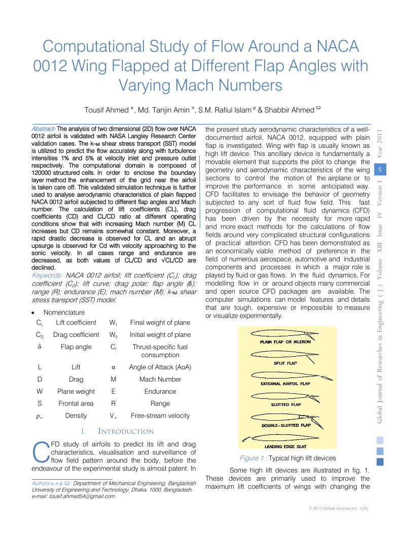
Figure 1 : Typical high lift devices
Some high lift devices are illustrated in fig. 1. These devices are primarily used to improve the maximum lift coefficients of wings with changing the
C
© 2013 Global Journals Inc. (US)
Volum
e X
III Issue
IV
Version
I
5
Year
013
2Globa
l Jo
urna
l of R
esea
rche
s in E
nginee
ring
(DDDD)
J
Tousif Ahmed α , Md. Tanjin Amin σ, S.M. Rafiul Islam ρ & Shabbir Ahmed Ѡ
characteristics for the cruising and high-speed flight
conditions. As a result, it is very important to understand the characteristics of the wing having different flap angles (δ) at different Mach number (M). Operating the aircraft at optimum flap angle at optimum velocity may result significant amount of fuel saving. The B-17 Flying Fortress, Cessna 152 and the helicopter Sikorsky S-61 SH-3 Sea King as well as horizontal and vertical axis wind turbines use NACA 0012 airfoil which place this specific airfoil under extensive research and study.
This study does not provide any experimental data for the flow over the flapped airfoil. Therefore, to reduce the scepticism associated the results obtained, the simulation process for the study is
validated instead.
In the validation course the results for flow over no flapped NACA 0012 is compared with published standard data by NASA [1], as nearly same computational method is used to study flapped NACA 0012 airfoil. Many researchers have studied aerodynamic characteristics of NACA 0012 using different methods and operating conditions. The Abbott and von Doenhoff data [7] were not tripped. The Gregory and O'Reilly data [10] were tripped, but were at a lower Re
of 3 million. Lift data are not affected too
significantly between 3 million and 6 million, but drag data are [11].
Selecting a proper turbulence model, the structure and use of a model to forecast the effects of turbulence, is
a crucial undertaking to study any sorts of
fluid flow. It should model the whole flow condition very accurately to get satisfactory results. Selection of wrong turbulence model often results worthless outcomes, as wrong model may not represent the actual physics of the flow. Turbulent flow dictates most flows of pragmatic engineering interest. Turbulence acts a key part in the determination of many relevant engineering parameters, for instance frictional drag, heat transfer, flow separation, transition from laminar to turbulent flow, thickness of boundary layers and wakes. Turbulence usually dominates all other flow phenomena and results in increasing energy dissipation, mixing, heat transfer, and
drag. In present study flow is
fully
developed turbulent and Reynolds number (Re) is set to
6×10⁶. Spallart-Allmaras, k-ε realizable, k-ω
standard
and k-ω Shear Stress Transport (SST) are primarily used
to model viscous turbulent model. However, these specific models are suitable for specific flow cases. Douvi C. Eleni [2] studied variation of lift and drag coefficients for different viscous turbulent model. His study shows that for flow around NACA 0012 airfoil k-ω
Shear Stress Transport (SST) model is the most accurate.
II.
Theoretical Background
Lowest flight velocities are encountered by an
airplane at takeoff or landing, two phases
that are most
perilous
for aircraft safety. The stalling speed Vstallis defined asthe slowest speed at which an airplane can fly in straight and level flight. Therefore, the calculation of Vstall, as well as aerodynamic methods of making Vstall
as
small as possible, is of vital importance.
The stalling velocity is readily obtained in terms of the maximum lift coefficient, as follows. From the definition of CL,
L= q∞SCL
= 1
2
ρ𝑉𝑉∞2SCL
Thus, V∞ =�2𝑊𝑊
𝜌𝜌∞𝑆𝑆𝐶𝐶𝐿𝐿 (1) [In case of steady level
flight, L=W]
Examining Eq. (1), we find that the
only alternative
to minimize V∞
is by maximizing
CLfor an
airplane of given weight and size at a given altitude. Therefore, stalling speed resembles
to the angle of
attack that yieldsCL,max:
Vstall =�2𝑊𝑊
𝜌𝜌∞𝑆𝑆𝐶𝐶𝐿𝐿 ,𝑚𝑚𝑚𝑚𝑚𝑚
(2)
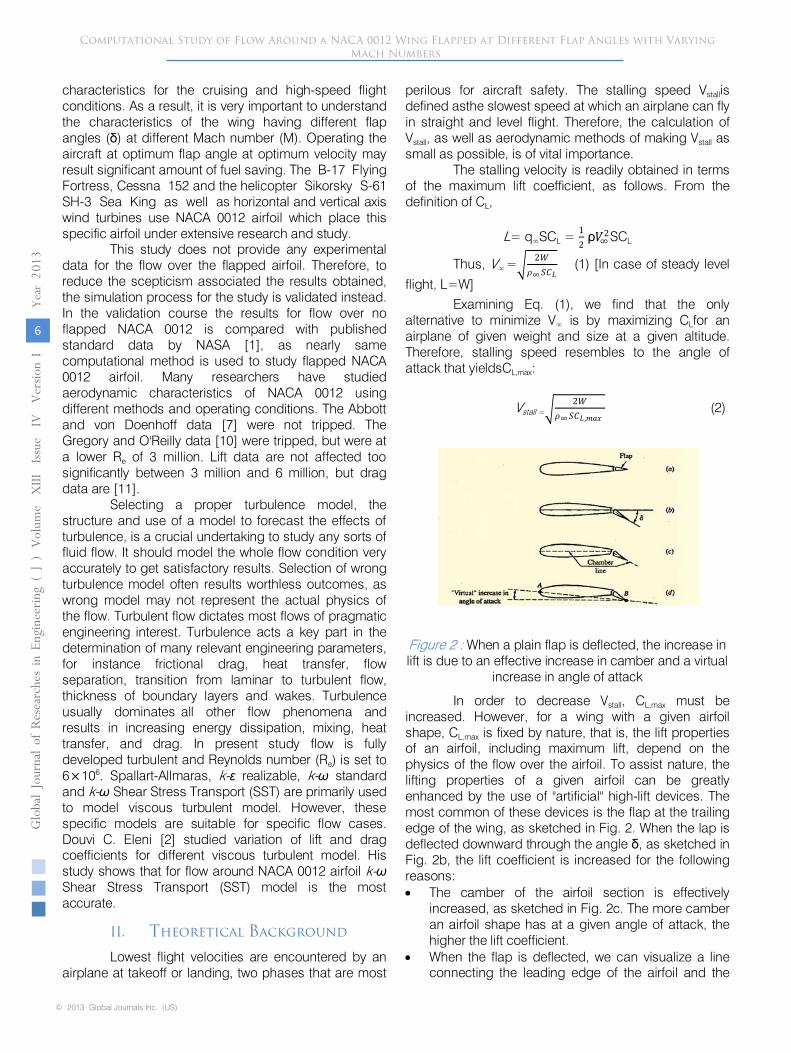
Figure 2 : When a plain flap is deflected, the increase in
lift is due to an effective increase in camber and a virtual increase in angle of attack
In order to decrease Vstall, CL,max
must be
increased. However, for a wing with a given airfoil shape, CL,max
is fixed by nature, that is, the lift properties
of an airfoil, including maximum lift, depend on the physics of the flow over the airfoil. To assist nature, the lifting properties of a given airfoil can be greatly enhanced by the use of "artificial" high-lift devices. The most common of these devices is the flap at the trailing edge of the wing, as sketched in Fig. 2. When the lap is deflected downward through the angle δ, as sketched in Fig. 2b, the lift coefficient is increased for the following reasons:
•
The camber of the airfoil section is effectively increased, as sketched in Fig. 2c. The more camber an airfoil shape has at a given angle of attack, the higher the lift coefficient.
•
When the flap is deflected, we can visualize a line connecting the leading edge of the airfoil and the
Computational Study of Flow Around a NACA 0012 Wing Flapped at Different Flap Angles with Varying Mach Numbers
© 2013 Global Journals Inc. (US)
Volum
e X
III Issue
IV
Version
I
6
Year
013
2Globa
l Jo
urna
l of R
esea
rche
s in E
nginee
ring
(DDDD)
J
trailing edge of the lap, points A and B, respectively, in Fig. 2d. Line AB constitutes a virtual chord line, rotated clockwise relative to the actual chord line of the airfoil, making the airfoil section with the deflected lap see a "virtual" increase in angle of attack. Hence, the lift coefficient is increased.
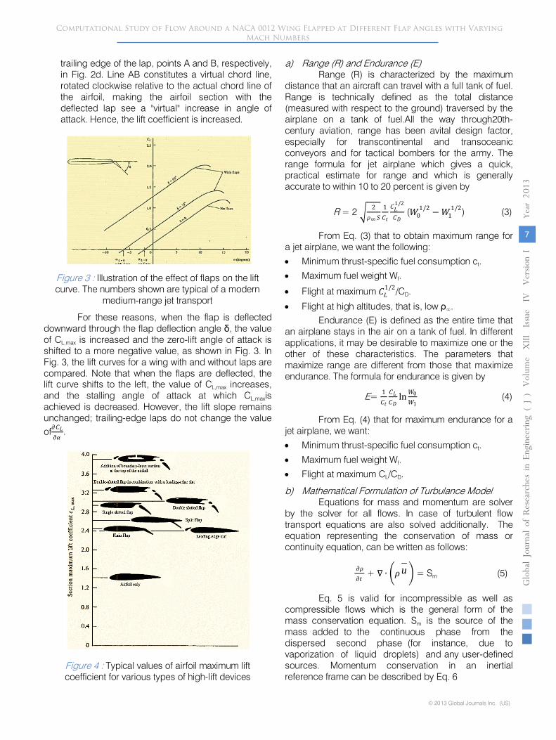
Figure 3 : Illustration of the effect of flaps on the lift
curve. The numbers shown are typical of a modern medium-range jet transport
For these reasons, when the flap is deflected downward through the flap deflection angle δ, the value of CL,max
is increased and the zero-lift angle of attack is
shifted to a more negative value, as shown in Fig. 3. In Fig. 3, the lift curves for a wing with and without laps are compared. Note that when the flaps are deflected, the lift curve shifts to the left, the value of CL,max
increases,
and the stalling angle of attack at which CL,maxis achieved is decreased. However, the lift slope remains unchanged; trailing-edge laps do not change the value of𝜕𝜕𝐶𝐶𝐿𝐿
𝜕𝜕𝜕𝜕.
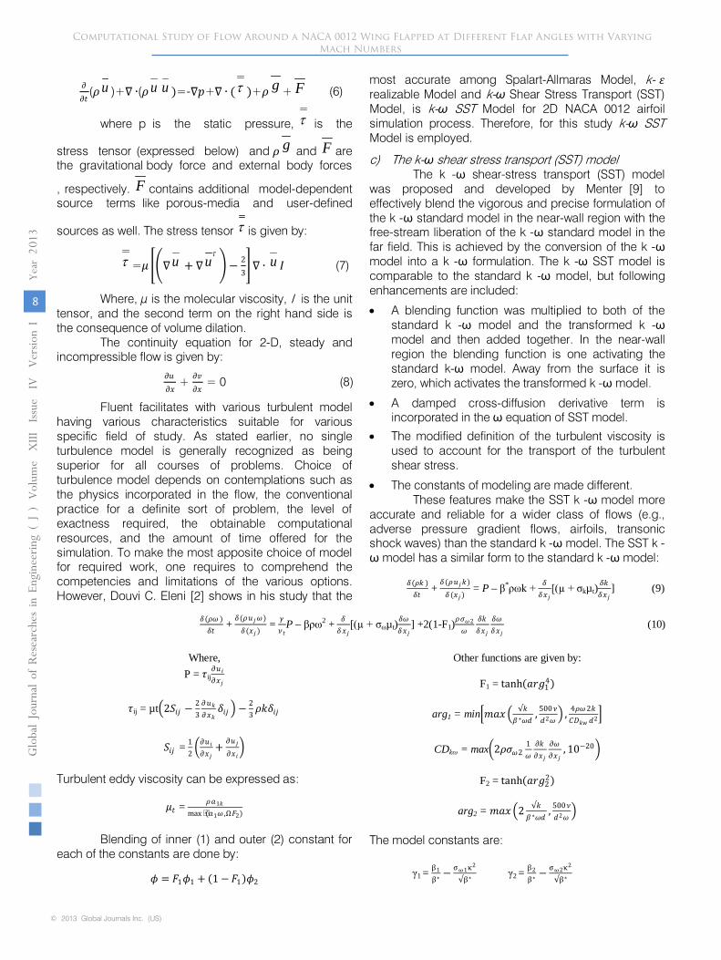
Figure 4 : Typical values of airfoil maximum lift coefficient for various types of high-lift devices
a)
Range (R) and Endurance (E)
Range (R) is characterized by the maximum distance that an aircraft can travel with a full tank
of fuel.
Range is technically defined as the total distance (measured with respect to the ground) traversed by the airplane on a tank of fuel.All the way through20th-century aviation, range has been avital
design factor,
especially for transcontinental and transoceanic conveyors
and for tactical
bombers for the army. The
range formula for jet airplane which gives a quick, practical estimate for range and which is generally accurate to within 10 to 20 percent is given by
R
= 2 � 2𝜌𝜌∞𝑆𝑆
1𝐶𝐶𝑡𝑡
𝐶𝐶𝐿𝐿1/2
𝐶𝐶𝐷𝐷
(𝑊𝑊0
1/2 −𝑊𝑊11/2) (3)
From Eq. (3) that to obtain maximum range for a jet airplane, we want the following:
•
Minimum thrust-specific fuel consumption ct.
•
Maximum fuel weight Wf.
•
Flight at maximum 𝐶𝐶𝐿𝐿1/2/CD.
•
Flight at high altitudes, that is, low ρ∞.
Endurance (E) is defined as the entire
time that
an airplane stays in the air on a tank of fuel. In different applications, it may be desirable to maximize one or the other of these characteristics. The parameters that maximize range are different from those that maximize endurance. The formula for endurance is given by
E= 1𝐶𝐶𝑡𝑡
𝐶𝐶𝐿𝐿𝐶𝐶𝐷𝐷
ln𝑊𝑊0𝑊𝑊1
(4)
From Eq. (4) that for maximum endurance for a jet airplane, we want:
•
Minimum thrust-specific fuel consumption ct.
•
Maximum fuel weight Wf.
•
Flight at maximum CL/CD.
b)
Mathematical Formulation of Turbulance Model
Equations for mass and momentum are solver by the solver for all flows. In case of turbulent flow transport equations are also solved additionally. The equation representing the conservation of mass or continuity equation, can be written as follows:
𝜕𝜕𝜌𝜌𝜕𝜕𝑡𝑡
+ ∇ ∙ �𝜌𝜌u �
= Sm
(5)
Eq. 5 is valid for incompressible as well as compressible flows which is the general form of the mass conservation equation. Sm
is the source of the mass added to the continuous phase from the dispersed second phase (for instance, due to vaporization of liquid droplets) and any user-defined sources. Momentum conservation in an inertial reference frame can be described by Eq. 6
Computational Study of Flow Around a NACA 0012 Wing Flapped at Different Flap Angles with Varying Mach Numbers
© 2013 Global Journals Inc. (US)
Volum
e X
III Issue
IV
Version
I
7
Year
013
2Globa
l Jo
urna
l of R
esea
rche
s in E
nginee
ring
(DDDD)
J
Computational Study of Flow Around a NACA 0012 Wing Flapped at Different Flap Angles with Varying Mach Numbers
© 2013 Global Journals Inc. (US)
Volum
e X
III Issue
IV
Version
I
8
Year
013
2Globa
l Jo
urna
l of R
esea
rche
s in E
nginee
ring
(DDDD)
J
𝜕𝜕𝜕𝜕𝑡𝑡
(𝜌𝜌u )+∇ ∙(𝜌𝜌u u )=-∇𝑝𝑝+∇ ∙ (τ )+𝜌𝜌 g + F (6)
where p is the static pressure, τ is the
stress tensor (expressed below) and 𝜌𝜌 g and F are the gravitational body force and external body forces
, respectively. F contains additional model-dependent source terms like porous-media and user-defined
sources as well. The stress tensor τ is given by:
τ =𝜇𝜇 ��∇u + ∇uτ�− 2
3�∇ ∙ u 𝐼𝐼 (7)
Where, µ is the molecular viscosity, I is the unit tensor, and the second term on the right hand side is the consequence of volume dilation.
The continuity equation for 2-D, steady and incompressible flow is given by:
𝜕𝜕𝜕𝜕𝜕𝜕𝑚𝑚
+ 𝜕𝜕𝜕𝜕𝜕𝜕𝑚𝑚
= 0 (8)
Fluent facilitates with various turbulent model having various characteristics suitable for various specific field of study. As stated earlier, no single turbulence model is generally recognized as being superior for all courses of problems. Choice of turbulence model depends on contemplations such as the physics incorporated in the flow, the conventional practice for a definite sort of problem, the level of exactness required, the obtainable computational resources, and the amount of time offered for the simulation. To make the most apposite choice of model for required work, one requires to comprehend the competencies and limitations of the various options. However, Douvi C. Eleni [2] shows in his study that the
most accurate among Spalart-Allmaras Model, k- 𝜀𝜀realizable Model and k-ω Shear Stress Transport (SST) Model, is k-ω SST Model for 2D NACA 0012 airfoil simulation process. Therefore, for this study k-ω SST Model is employed.
c) The k-ω shear stress transport (SST) modelThe k -ω shear-stress transport (SST) model
was proposed and developed by Menter [9] to effectively blend the vigorous and precise formulation of the k -ω standard model in the near-wall region with the free-stream liberation of the k -ω standard model in the far field. This is achieved by the conversion of the k -ωmodel into a k -ω formulation. The k -ω SST model is comparable to the standard k -ω model, but following enhancements are included:
• A blending function was multiplied to both of the standard k -ω model and the transformed k -ωmodel and then added together. In the near-wall region the blending function is one activating the standard k-ω model. Away from the surface it is zero, which activates the transformed k -ω model.
• A damped cross-diffusion derivative term is incorporated in the ω equation of SST model.
• The modified definition of the turbulent viscosity is used to account for the transport of the turbulent shear stress.
• The constants of modeling are made different. These features make the SST k -ω model more
accurate and reliable for a wider class of flows (e.g., adverse pressure gradient flows, airfoils, transonic shock waves) than the standard k -ω model. The SST k -ω model has a similar form to the standard k -ω model:
𝛿𝛿(𝜌𝜌𝜌𝜌 )𝛿𝛿𝑡𝑡
+ 𝛿𝛿(𝜌𝜌𝜕𝜕𝑗𝑗𝜌𝜌)𝛿𝛿 (𝑚𝑚𝑗𝑗 )
= P – β*ρωk + 𝛿𝛿𝛿𝛿𝑚𝑚𝑗𝑗
[(µ + σkµt)𝛿𝛿𝜌𝜌𝛿𝛿𝑚𝑚𝑗𝑗
] (9)
𝛿𝛿(𝜌𝜌𝜌𝜌 )𝛿𝛿𝑡𝑡
+ 𝛿𝛿(𝜌𝜌𝜕𝜕𝑗𝑗𝜌𝜌)𝛿𝛿(𝑚𝑚𝑗𝑗 )
= 𝛾𝛾𝜈𝜈𝑡𝑡
P – βρω2 + 𝛿𝛿𝛿𝛿𝑚𝑚𝑗𝑗
[(µ + σωµt)𝛿𝛿𝜌𝜌𝛿𝛿𝑚𝑚𝑗𝑗
] +2(1-F1)𝜌𝜌𝜎𝜎𝜌𝜌2𝜌𝜌
𝛿𝛿𝜌𝜌𝛿𝛿𝑚𝑚𝑗𝑗
𝛿𝛿𝜌𝜌𝛿𝛿𝑚𝑚𝑗𝑗
(10)
Where,P = 𝜏𝜏ij
𝜕𝜕𝜕𝜕𝑖𝑖𝜕𝜕𝑚𝑚𝑗𝑗
𝜏𝜏ij = µt�2𝑆𝑆𝑖𝑖𝑗𝑗 −23𝜕𝜕𝜕𝜕𝜌𝜌𝜕𝜕𝑚𝑚𝜌𝜌
𝛿𝛿𝑖𝑖𝑗𝑗 � −23𝜌𝜌𝜌𝜌𝛿𝛿𝑖𝑖𝑗𝑗
𝑆𝑆𝑖𝑖𝑗𝑗 = 12�𝜕𝜕𝜕𝜕𝑖𝑖𝜕𝜕𝑚𝑚𝑗𝑗
+ 𝜕𝜕𝜕𝜕𝑗𝑗𝜕𝜕𝑚𝑚𝑖𝑖�
Turbulent eddy viscosity can be expressed as:
𝜇𝜇𝑡𝑡 = 𝜌𝜌𝑚𝑚1𝜌𝜌max (𝑚𝑚1𝜌𝜌 ,Ω𝐹𝐹2)
Blending of inner (1) and outer (2) constant for each of the constants are done by:
𝜙𝜙 = 𝐹𝐹1𝜙𝜙1 + (1−𝐹𝐹1)𝜙𝜙2
Other functions are given by:
F1 = tanh(𝑚𝑚𝑎𝑎𝑎𝑎14)
arg1 = min�𝑚𝑚𝑚𝑚𝑚𝑚� √𝜌𝜌𝛽𝛽∗𝜌𝜌𝜔𝜔
, 500𝜈𝜈𝜔𝜔2𝜌𝜌
� , 4𝜌𝜌𝜌𝜌2𝜌𝜌𝐶𝐶𝐷𝐷𝜌𝜌𝑘𝑘 𝜔𝜔2�
CDkω = max�2𝜌𝜌𝜎𝜎𝜌𝜌21𝜌𝜌
𝜕𝜕𝜌𝜌𝜕𝜕𝑚𝑚𝑗𝑗
𝜕𝜕𝜌𝜌𝜕𝜕𝑚𝑚𝑗𝑗
, 10−20�
F2 = tanh(𝑚𝑚𝑎𝑎𝑎𝑎22)
arg2 = 𝑚𝑚𝑚𝑚𝑚𝑚�2 √𝜌𝜌𝛽𝛽∗𝜌𝜌𝜔𝜔
, 500𝜈𝜈𝜔𝜔2𝜌𝜌
�
The model constants are:
γ1 = β1β∗− σω1κ2
√β∗γ2 = β2
β∗− σω2κ2
√β∗
III.
Computational
Method
The well documented airfoil, NACA 0012, is utilized in this study. As NACA 0012
airfoil is symmetrical, theoretical lift at zero angle of attack, AoA (α) is zero. In order to validate the present simulation process, the operating conditions are mimicked to match the operating conditions of NASA
Langley Research Center validation cases [1].
Reynolds number for the simulations is Re=6x10⁶, the free
stream temperature is 300 K, which is the same as the ambient temperature. The density of the air at the given temperature is ρ
= 1.225kg/m3
and the viscosity is μ=1.7894×10⁻⁵ kg/ms. Flow for this Reynolds number can be labelled as incompressible. This is a supposition close to reality and there is no necessity to resolve the energy equation. A segregated, implicit solver, ANSYS Fluent 12, is utilized to simulate the problem. The airfoil profile is engendered in the Design Modeler and boundary conditions, meshes are created in the pre-processor ICEM-CFD. Pre-processor is a computer program that can be employed to generate 2D and 3D models, structured or unstructured meshes consisting of quadrilateral, triangular or tetrahedral elements. The resolution and density of the mesh is greater in regions where superior computational accuracy is needed, such as the near wall region of the airfoil.
As the first step of accomplishing a CFD simulation the influence of the mesh size on the solution results should be investigated. Mostly, more accurate numerical solution is obtained as more nodes are used, then again using added nodes also escalates the requisite computer memory and computational time. The determination of the proper number of nodes can be done by increasing the number of nodes until the mesh is satisfactorily fine so that further refinement does not change the results. Fig. 5 depicts the variation of coefficient of lift with number of grid cells at stall angle of attack (16°).
Figure 5 : Variation of lift coefficient with number of grid
cells [2]
120000 quadrilateral cells with C-type grid topology is
applied to establish a grid independent solution (Fig 6). From fig. 4 it is evident that 120000 cells are quite sufficient to get a stable and accurate result. Moreover, Douvi C. Eleni [2] was able to generate accurate results using only 80000 cells. The domain height and length is
set to approximately 25 chord lengths. This computational model is very small compared to that of NASA’s validation cases (fig. 7). Tominimize problems concomitant with the effect of far-field boundary (which can particularly influence drag and lift levels at high lift conditions), the far-field boundary in the grids provided have been located almost 500 chords away from the airfoil. But then again, simulation of NASA’s specification of the large computational domain requires very high computer memory. Furthermore, far-field boundary contributes very little on the result.
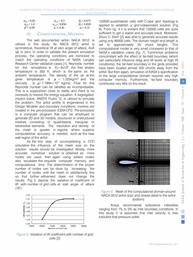
:
Mesh of the computational domain around NACA
0012 airfoil (top) and closed detail
to the airfoil (bottom)
Ansys recommends turbulence intensities ranging from 1% to 5% as inlet boundary conditions. In this study it is
assumed that inlet velocity is less turbulent that pressure outlet.
Computational Study of Flow Around a NACA 0012 Wing Flapped at Different Flap Angles with Varying Mach Numbers
© 2013 Global Journals Inc. (US)
Volum
e X
III Issue
IV
Version
I
9
Year
013
2Globa
l Jo
urna
l of R
esea
rche
s in E
nginee
ring
(DDDD)
J
𝜎𝜎𝜌𝜌1= 0.85 𝜎𝜎𝜌𝜌1= 0.5 𝛽𝛽1= 0.075𝜎𝜎𝜌𝜌2= 1.0 𝜎𝜎𝜌𝜌2= 0.856 𝛽𝛽2= 0.828𝛽𝛽∗= 0.09 𝜅𝜅 = 0.41 α1= 0.31
Figure 6
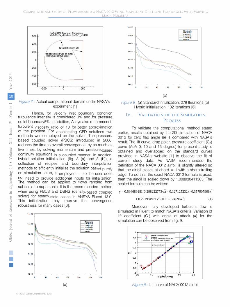
Figure 7 :
Actual computational domain under NASA’s experiment [1]
Hence, for velocity inlet boundary condition turbulence intensity is considered 1% and for pressure outlet boundary5%. In addition, Ansys also recommends turbulent
viscosity
ratio
of
10
for better approximation of the problem. For accelerating CFD solutions two methods were employed on the solver. The pressure-based coupled solver (PBCS) introduced in 2006, reduces the time to overall convergence, by as much as five times, by solving momentum and pressure-based continuity equations in a coupled manner. In addition, hybrid solution initialization (fig. 8 (a) and 8 (b)), a collection of recipes and boundary interpolation methods to efficiently initialize the solution based purely on simulation setup, is
employed —
so the user does not need to provide additional inputs for initialization. The method can be applied to flows ranging from subsonic to supersonic. It is the recommended method when using PBCS and DBNS (density-based coupled solver) for steady-state cases in ANSYS Fluent 13.0. This initialization may improve the convergence robustness for many cases [6].
(a)
(b)
Figure
8
:
(a) Standard Initialization, 279 Iterations (b) Hybrid Initialization, 102 Iterations [6]
IV.
Validation
of
the
Simulation
Process
To validate the computational method stated earlier, results obtained by the 2D simulation of NACA 0012 for zero flap angle (δ) is compared with NASA’s result. The lift curve, drag polar, pressure coefficient (CP) curve (AoA 0, 10 and 15 degree) for present study is
obtained and overlapped on the standard curves provided in NASA’s website [1] to observe the fit of current study data. As NASA recommended the definition of the NACA 0012 airfoil is slightly
altered so that the airfoil closes at chord = 1 with a sharp trailing edge. To do this, the exact NACA 0012 formula is used, then the airfoil is scaled down by 1.008930411365. The scaled formula can be written:
y = 0.594689181[0.298222773√𝑚𝑚
-
0.127125232x -0.357907906x2
+ 0.291984971x3
-
0.105174696x4] (1)
Computational Study of Flow Around a NACA 0012 Wing Flapped at Different Flap Angles with Varying Mach Numbers
© 2013 Global Journals Inc. (US)
Volum
e X
III Issue
IV
Version
I
10
Year
013
2Globa
l Jo
urna
l of R
esea
rche
s in E
nginee
ring
(DDDD)
J
Moreover, fully developed turbulent flow issimulated in Fluent to match NASA’s criteria. Variation of lift coefficient (CL) with angle of attack (α) for the simulation can be observed from fig. 9.
Figure 9 : Lift curve of NACA 0012 airfoil
From
-16 degree AoA to 16 degree AoA the lift curve is almost linear. Throughout this regime no separation occurs and flow remains attached to the airfoil. At stall AoA lift coefficient is reduced drastically due to intense flow separation generation. Slight
deviation from Abbott and Von Doenhoff’s [7] unstripped experimental results occurs (almost 3%), as the computational
domain of the current study is
nearly 1/20th
of the original computational domain under experiment of NASA.
Fig. 10 depicts the conformation of drag polar of current validation study with NASA’s validation cases. Present study results tie reasonably well with Abbott and Von Doenhoff’s [7] unstripped experimental results.
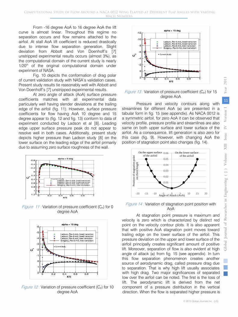
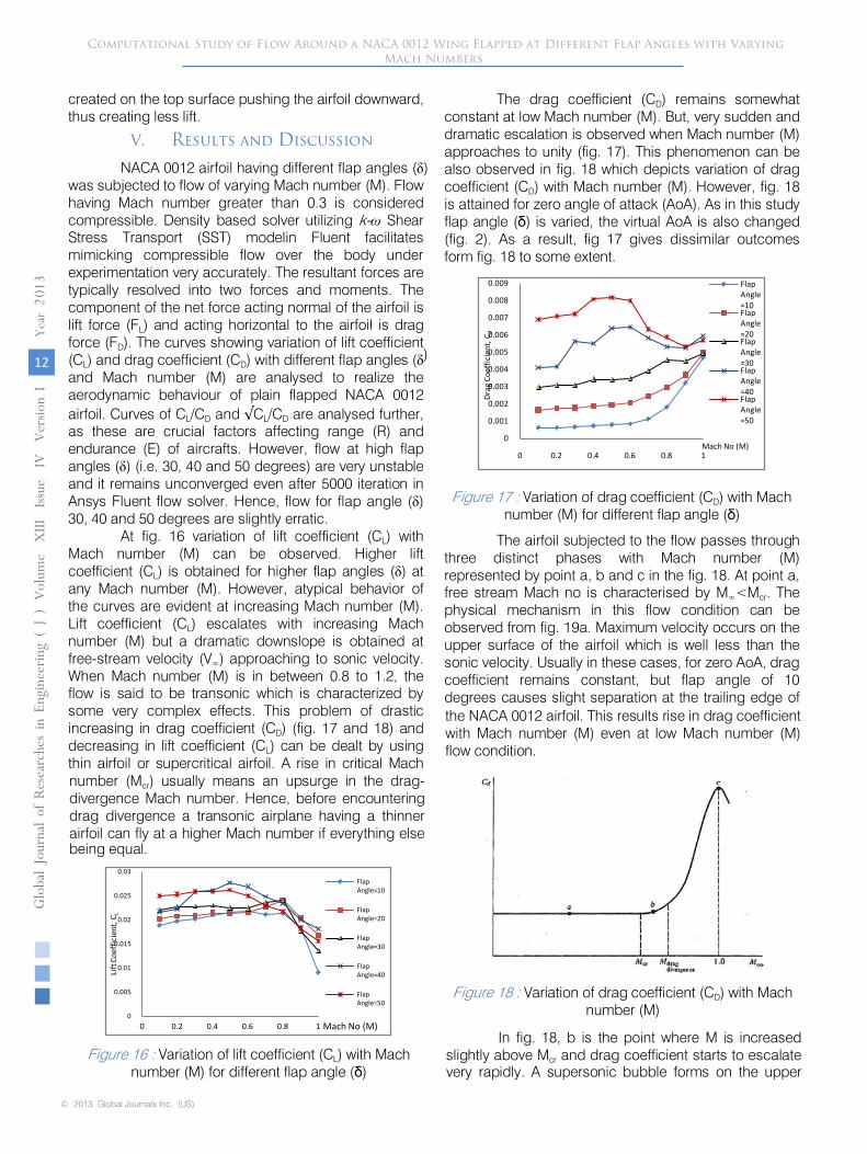
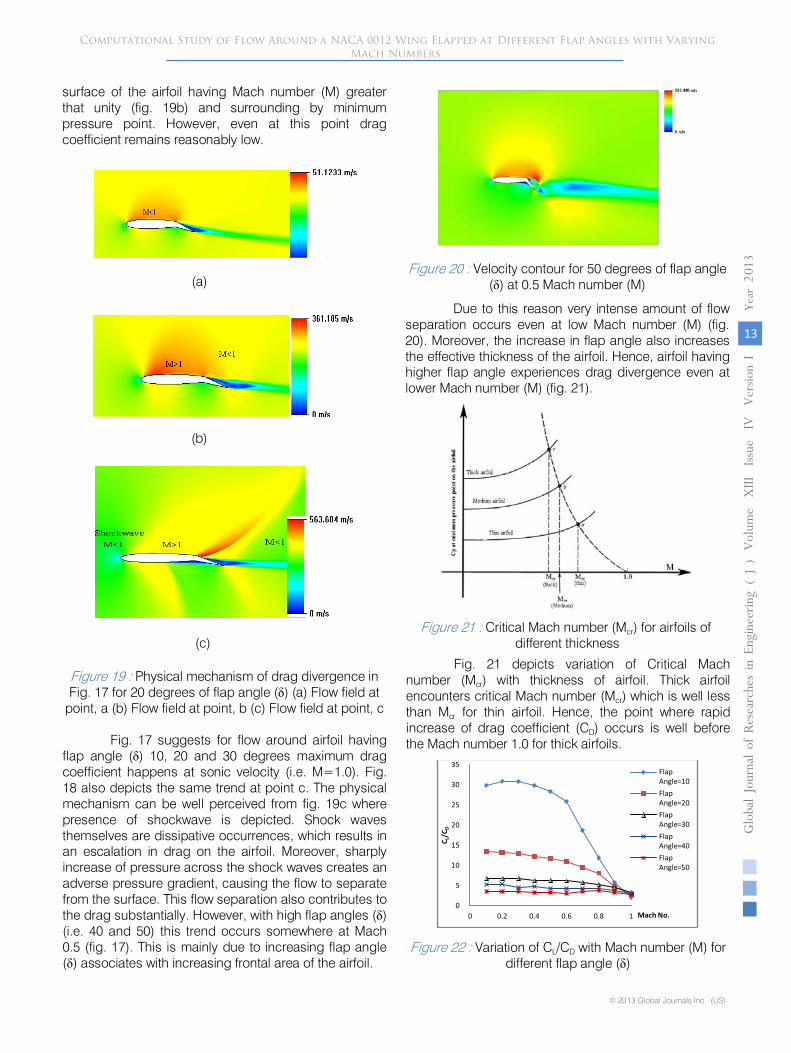
At zero angle of attack (AoA) surface pressure coefficients matches with all experimental data particularly well having slender deviations at the trailing edge of the airfoil (fig. 11). However, surface pressure coefficients for flow having AoA 10 degree and 15 degree appear to (fig. 12 and fig. 13) conform to data of experiment conducted by Ladson et al [8]. Leading edge upper surface pressure peak do not appear to resolve well in both cases. Additionally, present study depicts higher pressure than Ladson study [8] on the lower surface on the leading edge of the airfoil primarily due to assuming zero surface roughness of the wall.
Figure
11
:
Variation of pressure coefficient (CP) for 0 degree AoA
Figure
12
:
Variation of pressure coefficient (CP) for 10 degree AoA
Figure
13
:
Variation of pressure coefficient (CP) for 15 degree AoA
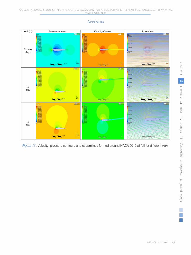
Pressure and velocity contours along with streamlines for different AoA (α) are presented in a tabular form in fig. 15
(see
appendix). As NACA 0012 is a symmetric airfoil, for zero AoA it can be
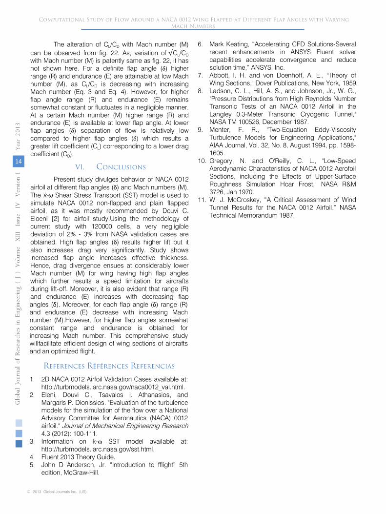
observed that velocity profile, pressure profile and streamlines are also same on both upper surface and lower surface of the airfoil. As a consequence, lift generation is also zero for this case (fig. 9). However, with changing AoA the position of stagnation point also changes (fig. 14).
Figure 14
:
Variation of stagnation point position with AoA
0
0.01
0.02
0.03
0.04
0.05
0.06
-20 -15 -10 -5 0 5 10 15 20
Posit
ion
of st
agna
ti on
poin
ton
chor
d le
ngth
Angle of Attack (AoA)
On the lower surfaceof the airfoil
On the upper surfaceof the airfoil
Computational Study of Flow Around a NACA 0012 Wing Flapped at Different Flap Angles with Varying Mach Numbers
© 2013 Global Journals Inc. (US)
Volum
e X
III Issue
IV
Version
I
11
Year
013
2Globa
l Jo
urna
l of R
esea
rche
s in E
nginee
ring
(DDDD)
J
At stagnation point pressure is maximum and velocity is zero which is characterized by distinct red point on the velocity contour plots. It is also apparent that with positive AoA stagnation point moves toward trailing edge on the lower surface of the airfoil. This pressure deviation on the upper and lower surface of the airfoil principally creates significant amount of positive lift. Moreover, separation of flow is also evident at high angle of attack (α) from fig. 15 (see appendix). In turn this flow separation phenomenon creates another source of aerodynamic drag, called pressure drag due to separation. That is why high lift usually associates with high drag. Two major significances of separated low over the airfoil can be noted. The first is the loss of lift. The aerodynamic lift is derived from the net component of a pressure distribution in the vertical direction. When the flow is separated higher pressure is
created on the top surface pushing the airfoil downward, thus creating less lift.
V.
Results
and
Discussion
NACA 0012 airfoil having different flap angles (δ) was subjected to flow of varying Mach number (M). Flow having Mach number greater than 0.3 is
considered compressible. Density based solver utilizing k-ω
Shear Stress Transport (SST) modelin Fluent facilitates mimicking compressible flow over the body under experimentation very accurately. The resultant forces are typically resolved into two forces and moments. The component of the net force acting normal of the airfoil is lift force (FL) and acting horizontal to the airfoil is drag force (FD).
The curves showing variation of lift coefficient (CL) and drag coefficient (CD) with different flap angles (δ)
and Mach number (M) are analysed to realize the aerodynamic behaviour of plain flapped NACA 0012 airfoil. Curves of CL/CD
and √CL/CD
are analysed further, as these are crucial factors affecting range (R) and endurance (E) of aircrafts. However, flow at high flap angles (δ) (i.e. 30, 40 and 50 degrees) are very unstable and it remains unconverged even after 5000 iteration in Ansys Fluent flow solver. Hence, flow for flap angle (δ) 30, 40 and 50 degrees are slightly erratic.
At fig. 16 variation of lift coefficient (CL) with Mach number (M) can be observed. Higher lift coefficient (CL) is obtained for higher flap angles (δ) at any Mach number (M). However, atypical behavior of the curves are evident at increasing Mach number (M). Lift coefficient (CL) escalates with increasing Mach number (M) but a dramatic downslope is obtained at free-stream velocity (V∞) approaching to sonic velocity. When Mach number (M) is in between 0.8 to 1.2, the flow is said to be transonic which is characterized by some very complex effects. This problem of drastic increasing in drag coefficient (CD)
(fig. 17 and 18) and decreasing in lift coefficient (CL) can be dealt by using thin airfoil or supercritical airfoil. A rise in critical Mach number (Mcr) usually means an upsurge in the drag-divergence Mach number. Hence, before encountering drag divergence a transonic airplane having a thinner airfoil can fly at a higher Mach number if everything else being equal.
The drag coefficient (CD)
remains somewhat constant at low Mach number (M). But, very sudden and dramatic escalation is observed when Mach number (M) approaches to unity (fig. 17). This phenomenon can be also observed in fig. 18 which depicts variation of drag coefficient (CD) with Mach number (M). However, fig. 18 is attained for zero angle of attack (AoA). As in this study flap angle (δ) is varied, the virtual AoA is also changed (fig. 2). As a result, fig 17 gives
dissimilar outcomes form fig. 18 to some extent.
Figure
17
:
Variation of drag coefficient (CD) with Mach number (M) for different flap angle (δ)
The airfoil subjected to the flow passes through three distinct phases with Mach number (M) represented by point a, b and c in the fig. 18. At point a, free stream Mach no is characterised by M∞<Mcr. The physical mechanism in this flow condition can be observed from fig. 19a. Maximum velocity occurs on the upper surface of the airfoil which is well less than the sonic velocity. Usually in these cases, for zero AoA, drag coefficient remains constant, but flap angle of 10
degrees causes slight separation at the trailing edge of
0
0.001
0.002
0.003
0.004
0.005
0.006
0.007
0.008
0.009
0 0.2 0.4 0.6 0.8 1
Flap Angle=10Flap Angle=20Flap Angle=30Flap Angle=40Flap Angle=50
Mach No (M)
Drag
Coef
ficie
nt, C
d
Computational Study of Flow Around a NACA 0012 Wing Flapped at Different Flap Angles with Varying Mach Numbers
© 2013 Global Journals Inc. (US)
Volum
e X
III Issue
IV
Version
I
12
Year
013
2Globa
l Jo
urna
l of R
esea
rche
s in E
nginee
ring
(DDDD)
J
Figure 16 : Variation of lift coefficient (CL) with Mach number (M) for different flap angle (δ)
0
0.005
0.01
0.015
0.02
0.025
0.03
0 0.2 0.4 0.6 0.8 1
Lift
Coe
ffic
ient
, CL
Mach No (M)
Flap Angle=10
Flap Angle=20
Flap Angle=30
Flap Angle=40
Flap Angle=50
the NACA 0012 airfoil. This results rise in drag coefficient with Mach number (M) even at low Mach number (M) flow condition.
Figure 18 : Variation of drag coefficient (CD) with Mach number (M)
In fig. 18, b is the point where M is increased slightly above Mcr and drag coefficient starts to escalate very rapidly. A supersonic bubble forms on the upper
surface of the airfoil having Mach number (M) greater that unity (fig. 19b) and surrounding by minimum pressure point. However, even at this point drag coefficient remains reasonably low.
(a)
(b)
(c)
Figure
19
:
Physical mechanism of drag divergence in Fig. 17 for 20 degrees of flap angle (δ) (a) Flow field at
point, a (b) Flow field at point, b (c) Flow field at point, c
Fig. 17 suggests for flow around airfoil having flap angle (δ) 10, 20 and 30 degrees maximum drag coefficient happens at sonic velocity (i.e. M=1.0). Fig. 18 also depicts the same trend at point c. The physical mechanism can be well perceived from fig. 19c where presence of shockwave is depicted. Shock waves themselves are dissipative occurrences, which results in an escalation in drag on the airfoil. Moreover, sharply increase of pressure across the shock waves creates an adverse pressure gradient, causing the flow to separate from
the surface. This flow separation also contributes to the drag substantially. However, with high flap angles (δ) (i.e. 40 and 50) this trend occurs somewhere at Mach 0.5 (fig. 17). This is mainly due to increasing flap angle (δ) associates with increasing
frontal area of the airfoil.
Figure 20
:
Velocity contour for 50 degrees of flap angle (δ) at 0.5 Mach number (M)
Due to this reason very intense amount of flow separation occurs even at low Mach number (M) (fig. 20). Moreover, the increase in flap angle
also increases the effective thickness of the airfoil. Hence, airfoil having higher flap angle experiences drag divergence even at lower Mach number (M) (fig. 21).
Figure
21 :
Critical Mach number (Mcr) for airfoils of different thickness
Computational Study of Flow Around a NACA 0012 Wing Flapped at Different Flap Angles with Varying Mach Numbers
© 2013 Global Journals Inc. (US)
Volum
e X
III Issue
IV
Version
I
13
Year
013
2Globa
l Jo
urna
l of R
esea
rche
s in E
nginee
ring
(DDDD)
J
Fig. 21 depicts variation of Critical Mach number (Mcr) with thickness of airfoil. Thick airfoil encounters critical Mach number (Mcr) which is well less than Mcr for thin airfoil. Hence, the point where rapid increase of drag coefficient (CD) occurs is well before the Mach number 1.0 for thick airfoils.
Figure 22 : Variation of CL/CD with Mach number (M) for different flap angle (δ)
0
5
10
15
20
25
30
35
0 0.2 0.4 0.6 0.8 1
C L/C
D
Mach No.
Flap Angle=10Flap Angle=20Flap Angle=30Flap Angle=40Flap Angle=50
The alteration of CL/CD
with Mach number (M) can be observed from fig. 22. As, variation of √CL/CD
with Mach number (M) is patently same as fig. 22, it has not shown here. For a definite flap angle (δ) higher range (R) and endurance (E) are attainable at low Mach number (M), as CL/CD
is decreasing with increasing Mach number (Eq. 3 and Eq. 4). However,
for higher flap angle range (R) and endurance (E) remains somewhat constant or fluctuates in a negligible manner. At a certain Mach number (M) higher range (R) and endurance (E) is available at lower flap angle. At lower flap angles (δ) separation of flow
is relatively low compared to higher flap angles (δ) which results a greater lift coefficient (CL) corresponding to a lower drag coefficient (CD).
VI.
Conclusions
Present
study divulges
behavior of NACA 0012 airfoil at different flap angles (δ) and Mach numbers
(M).
The k-ω
Shear Stress Transport (SST) model
is used to simulate NACA 0012 non-flapped and plain flapped airfoil, as it was mostly recommended by Douvi C. Eloeni
[2]
for airfoil study.Using the methodology of current study
with 120000 cells,
a very negligible deviation of 2% -
3% from NASA validation cases are obtained. High flap angles (δ) results higher lift but it also increases drag very significantly. Study shows increased flap angle increases effective thickness. Hence, drag divergence ensues at considerably lower Mach number (M)
for wing
having high flap angles
which further results a speed limitation for aircrafts during lift-off. Moreover, it is
also evident that range (R) and endurance (E) increases with decreasing flap
angles
(δ). Moreover, for each flap angle (δ) range (R) and endurance (E) decrease with increasing Mach number (M).However, for higher flap angles somewhat constant range and endurance is obtained for increasing Mach number. This comprehensive study willfacilitate
efficient design of wing sections
of aircrafts
and an optimized flight.
References Références Referencias
1.
2D NACA 0012 Airfoil Validation Cases available at: http://turbmodels.larc.nasa.gov/naca0012_val.html.
2.
Eleni, Douvi C., Tsavalos I. Athanasios, and Margaris P. Dionissios. "Evaluation of the turbulence models for the simulation of the flow over a National Advisory Committee for Aeronautics (NACA) 0012 airfoil." Journal of Mechanical Engineering Research
4.3 (2012): 100-111.
3.
Information on k-ω
SST model available at: http://turbmodels.larc.nasa.gov/sst.html.
4.
Fluent 2013 Theory Guide.
5.
John D Anderson, Jr. “Introduction to fflight” 5th edition, McGraw-Hill.
6.
Mark Keating, “Accelerating CFD Solutions-Several recent enhancements in ANSYS Fluent solver capabilities accelerate convergence and reduce solution time,” ANSYS, Inc.
7.
Abbott, I. H. and von Doenhoff, A. E., "Theory of Wing Sections," Dover Publications, New York, 1959.
8.
Ladson, C. L., Hill, A. S., and Johnson, Jr., W.
G., "Pressure Distributions from High Reynolds Number Transonic Tests of an NACA 0012 Airfoil in the Langley 0.3-Meter Transonic Cryogenic Tunnel," NASA TM 100526, December 1987.
9.
Menter, F. R., "Two-Equation Eddy-Viscosity Turbulence Models for Engineering
Applications," AIAA Journal, Vol. 32, No. 8, August 1994, pp. 1598-1605.
10.
Gregory, N. and O'Reilly, C. L., "Low-Speed Aerodynamic Characteristics of NACA 0012 Aerofoil Sections, including the Effects of Upper-Surface Roughness Simulation Hoar Frost," NASA R&M 3726, Jan 1970.
11.
W. J. McCroskey, “A Critical Assessment of Wind Tunnel Results for the NACA 0012 Airfoil.” NASA Technical Memorandum 1987.
Computational Study of Flow Around a NACA 0012 Wing Flapped at Different Flap Angles with Varying Mach Numbers
© 2013 Global Journals Inc. (US)
Volum
e X
III Issue
IV
Version
I
14
Year
013
2Globa
l Jo
urna
l of R
esea
rche
s in E
nginee
ring
(DDDD)
J
Computational Study of Flow Around a NACA 0012 Wing Flapped at Different Flap Angles with Varying Mach Numbers
© 2013 Global Journals Inc. (US)
Volum
e X
III Issue
IV
Version
I
15
Year
013
2Globa
l Jo
urna
l of R
esea
rche
s in E
nginee
ring
(DDDD)
J
Appendix
AoA (α) Pressure contour Velocity Contour Streamlines
0 (zero)deg.
10deg.
15deg.
Figure 15 : Velocity, pressure contours and streamlines formed around NACA 0012 airfoil for different AoA

This page is intentionally left blank
Computational Study of Flow Around a NACA 0012 Wing Flapped at Different Flap Angles with Varying Mach Numbers
© 2013 Global Journals Inc. (US)
Volum
e X
III Issue
IV
Version
I
16
Year
013
2Globa
l Jo
urna
l of R
esea
rche
s in E
nginee
ring
(DD DD)
J

![ANALISIS 2D AIRFOIL NACA 4412 MENGGUNAKAN1].pdfthe airfoil NACA 4412. At the stall angle subsonic flow has a higher lift coefficient value of 1,17290 compared with supersonic flow](https://img.pdfslide.net/doc/110x75/61329c48dfd10f4dd73a8fdb/analisis-2d-airfoil-naca-4412-menggunakan-1pdf-the-airfoil-naca-4412-at-the-stall.jpg)