MCAT Institute

Final Report94-003

Computational Study Of GenericHypersonic Vehicle Flow Field

Johnny R. Narayan

May 1994 NCC2-715

MCAT Institute3933 Blue Gum Drive

San Jose, CA 95127

https://ntrs.nasa.gov/search.jsp?R=19940029771 2018-06-27T20:59:46+00:00Z

WORK STATEMENT

gllllllt MUllS

The co-operative agreement was initiated for achieving the following:

1. Carry out a tip-to-tail computation of the flow field of a generic hypersonic vehicle in the

power-on configuration. The main focus of the task was to establish and demonstrate a solution

procedure/strategy that would be useful for solving the entire flow field associated with an

airbreathing hypersonic vehicle. The plan was to utilize available Computational Fluid

Dynamics (CFD) codes for this purpose rather than generating a new specialized CFD solver.

This would need modifications to the codes to enhance their capabilities in terms of accurate

models for physical features such as turbulence, finite rate chemistry, improved boundary

conditions etc.

2. Develop and demonstrate a turbulence-chemistry interactions model applicable for high-

speed reacting flows involving finite rate chemistry.

The following sections describe the milestones achieved, work in progress and

suggestions for future work pertaining to the items described above. In this report,

bibliographical references to the physical models such as the turbulence models, thermodynamic

models, finite rate chemistry models etc. and CFD codes used are omitted. However, these

references can easily be obtained from the attached publications pertaining to the present task.

HYPERSONIC TIP-TO.TAIL COMPUTATION

The geometry of the generic hypersonic vehicle configuration was provided by Dr. Tom

Edwards of the Computational Aerosciences Branch, Fluid Dynamics Division at NASA Ames

Research Center. The geometric data included body definitions and preliminary grids for the

forebody (nose cone excluded), midsection (propulsion system excluded) and afterbody sections.

This data was to be augmented by the nose section geometry (blunt conical section mated with

the non circular cross section of the forebody initial plane) along with a grid and a detailed

supersonic combustion ramjet (scramjet) geometry (inlet and combustor) which should be

merged with the nozzle portion of the afterbody geometry. The solutions were to be obtained by

using a Navier-Stokes (NS) code such as TUFF for the nose portion, a Parabolized Navier

Stokes (PNS) solver such as the UPS and STUFF codes for the forebody, a NS solver with

finite rate hydrogen-air chemistry capability such as TUFF and SPARK for the scramjet and a

suitable solver (NS or PNS) for the afterbody and external nozzle flows. Proper interfacing was

to be maintained between the solutions of the different sections.

NOSE SECTION

The nose is assumed to be a blunt one in the present computations in keeping with the

accepted designs for an airbreathing hypersonic vehicle. As mentioned above, the nose section is

a blunt-nosed cone at zero angle of attack. An axisymmetric grid was generated for the nose

section using the graphic utility VG available on workstation win35. The TUFF code was used

to solve the flow field upto the axial location corresponding to the fin'st plane of the forebody

geometry. Finite rate nonequilibrium air-chemistry model was used along with a two-equation

turbulence (k-epsilon) model. The flow Mach number was 15 and the Reynolds number based on

unit length was 1,700,000. The surface of the body was assumed to be maintained at a constant

temperature of 243.4 K. No-slip boundary conditions were used at the body surface. The

solutions were then interpolated onto the first plane of the forebody grid.

FOREBODY

Computations were carried out using the PNS solvers STUFF and UPS in order to

ascertain that these codes were equivalent as for as the present application was concerned. The

nose-section solution was used along with the forebody grid for this purpose. The solutions were

obtained for the flow field around the entire forebody upto the inlet location. Baldwin-Lomax

turbulence model was used since the version of the UPS code used does not have the two-

equationturbulencemodelcapability. Thesolutionswerecompared(temperature,velocitiesandpressure)and found to be in excellentagreement. Sincethe TUFF and STUFF codeshave

similar structure and physical models, it was decided to use them for the NS and PNS

applications,respectively,unlessconditionsdictatedtheutilization of a different code suchasSPARK. This would beextremelyusefulin interfacingsolutionsbetweendifferent sectionsofthevehicle.

Sincethenosesectionwasaconical bodywith circularcrosssection,it wasnecessarytogenerateaseriesof crosssectionsatdesignatedintervalswhichchangedin shapefrom acircle to

that of thefirst crosssectionof theforebodygrid. A threedimensionalgrid that bridgedthe last

planeof the nosesectionwith the first planeof the forebodywas then generatedusing thesesurfacedefinitions (crosssections)andwascombinedwith the given forebodygrid to form thenewthreedimensionalgrid for theforebodyflow field solutions. ThesesolutionswereobtainedbyusingthespacemarchingPNSsolverSTUFF. Thenose-sectionsolutionswereusedasinitial

data for this purpose.The two-equation(k-epsilon)turbulencemodel including low-Reynolds

numbertermsto accountfor thenear-wall flow field wasusedandthe finite rate air-chemistrymodelof the nosesectionwasmaintained. Eventhoughthe turbulencefield wasnot oneof the

primary targets in thesecomputations, turbulencemodeling at the two-equation level wasmaintainedin anticipationof the inlet/combustorflow simulationswhich require the useof the

physically more realistic two-equationmodel ratherthan the simpleand easyto usealgebraicBaldwin-Lomax model. As a result, the computationsrequired more computerresources.Typical results(compositesincethe full computationaldataat all the x-locationscould not be

stored)are shown in the figures at the end of the report. Computationally, there were no

unforeseendifficulties in obtainingthesesolutions. This task was completedin September,1992.

INLET

The inlet computations represent the critical (bottleneck) part of the entire tip-to-tail

solutions. The difficulty was associated with the proper choice of a realistic inlet configuration

at the same time minimizing the computational effort which utilized the available resources in an

efficient manner. The geometric restrictions imposed by the limited length of the entire scramjet

propulsion system to achieve the power requirements for the hypersonic flight is a major factor

to be considered here. The mixing between the incoming airflow and the injected fuel dominates

the flow field and the mixing efficiency plays a major role in determining the dimensions and

geometry of the inlet. Also, physical aspects of the flow such as inlet unstart, flow spillage at

thecowl locationto maintaintheproperair flow etc.arekeyfactorsthatmustbedealtwith in the

solutions. The solutions are computationally intensive, requiring an enormousamount of

computationalresources.Sincethe incomingforebodyflow is threedimensional,the inlet flowsolutionsalsorequirefully threedimensionalanalyses.

The computational effort was divided into a series of tasks. First, an inlet

configurationhadbeselected.Sincethepresentwork was meant to be a demonstration type with

the purpose of establishing a solution procedure/strategy for carrying out tip-to-tail

computations, it was decided to use a multi-module scramjet inlet for the present task. This

would conform to the widely accepted inlet configurations being used in research and

development efforts carried out at a majority of establishments working in the area of hypersonic

flight. In order to reduce the computational effort thus minimizing the demand for computational

resources, a three-module configuration that spans the entire undersurface of the vehicle was

chosen for the present task. The next task was concerned with the selection of the geometric

configuration of each inlet module. Once again, taking into account the realistic configurations

and keeping with the aim of minimizing computational effort, a swept-back twin strutted module

with side-wall compression was chosen for the present task. A sweep angle of 30 degrees was

chosen along with a strut angle of 6 degrees. A schematic view of the inlet module is given in

the figures.

The above mentioned choice for the inlet geometry immediately introduced a new

problem. This problem was associated with the choice of the particular CFD solver to be used

for the solutions. The multiple-module configuration with the cowl plate located downstream of

the strut tip introduced a variety of boundary conditions at different locations in the flow field.

For example, a typical module has solid walls on three of the six boundary surfaces that define

its geometry (omitting for the time being factors such as injection at solid walls). The inlet and

exit boundaries pose no serious problems also. However, the fourth boundary that is aligned

with the cowl plate surface involves both no-slip and flow-through conditions which are not easy

to implement in the CFD codes under consideration. Also, due to the presence of the struts

inside the flow region, an enormous grid (single, 3-D) would be required to have any chance at

obtaining a realistic solution. The grid needed would be impractical to be used with a NS solver.

As a result, a multi-block NS solver that includes all the physical models used for the computing

the flow field around the forebody was needed. The multi-block version of the TUFF code

became available at that time and hence was selected as the CFD solver for the inlet flow

analysis. However, the problems associated with mixed boundary conditions, alluded to earlier,

still remained requiring modification of the multi-block TUFF code to account for mixed

boundary conditions. These modifications were incorporated in the solver which required

considerableresourcesin termsof manpower as well as computational resources for validation.

The changes led to a system by which different boundary conditions (from among the original

options provided in the solver) could be specified at every grid point on the six boundary

surfaces.

The fuel of choice for the present case is hydrogen. However, the chemistry model in the

TUFF code was for hydrocarbon-air combustion. This led to further modifications to the code

whereby a hydrogen-air (finite rate) chemistry model involving nine species (hydrogen, oxygen,

water, OH, H, O and nitrogen) and 20 reaction steps (suggested by the NASP Technical

Committee) was incorporated. Also, thermodynamic models valid over a wider range of

temperature than before was incorporated (by the author of the code). Even though chemical

reactions involving combustion are not expected in the inlet, the chemistry model is included for

the inlet flow solutions so as to be consistent with the combustor solutions which would follow.

The solution domain is divided into adjoining blocks/zones with distinct boundary

conditions. This is done in such a way that the occurrence of mixed boundary conditions along

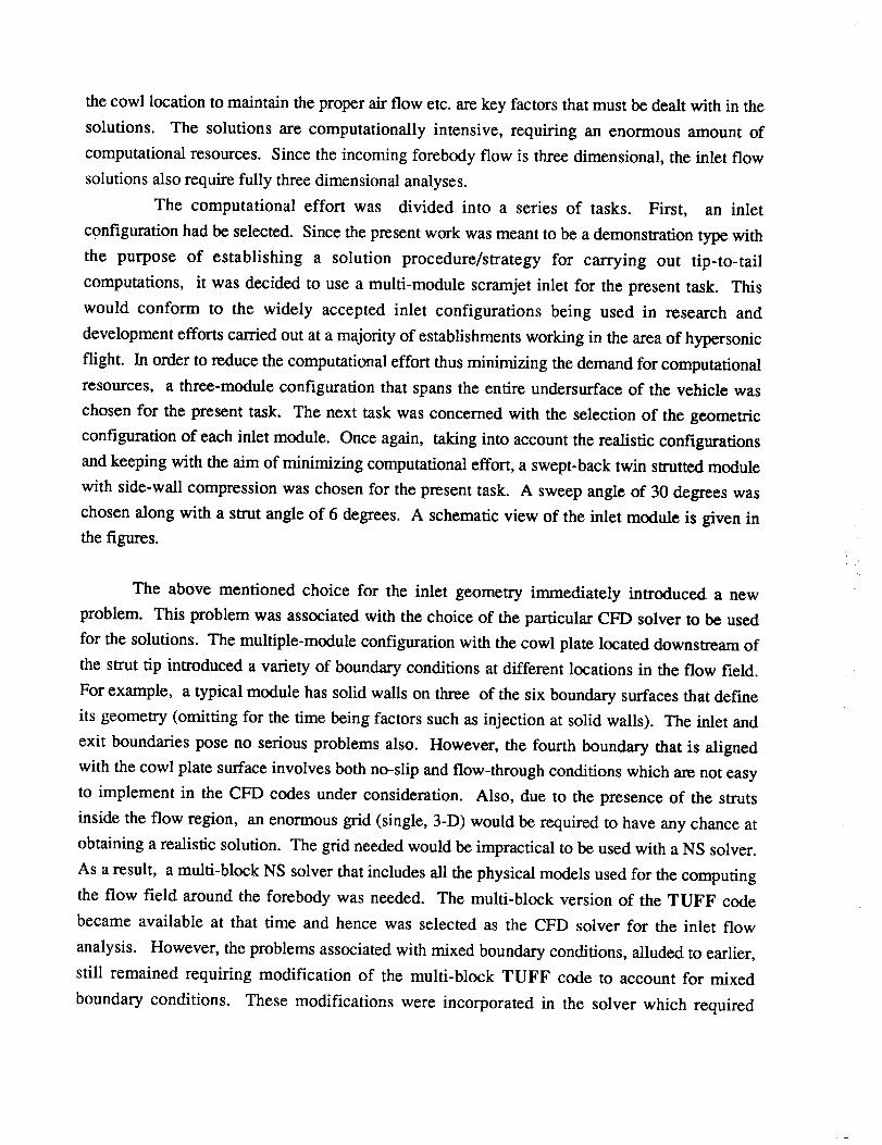
the boundaries is kept to a minimum. A multi-block grid involving 7 blocks was generated for

the solutions. A schematic of the block arrangement is shown in the figures along with a

representation of the grid system. The solution of the flow in the inlet represents the most

computationally intensive part of the entire solution process. The flow is both external and

internal involving strong and weak shocks/expansions in the domain. The precompressed air

from the forebody (undersurface, mainly) enters the multiple module inlet and undergoes further

changes due to the geometry of the inlet. There is flow spillage at the cowl requiring to pay

extra attention to the grid there.

Solution of the inlet flow was carded out over a long period of real time. One of the

reasons for this was the fact that the computer resources ran out in 1992 about four months

before the start of the next account year, virtually stopping the computationally intensive inlet

flow solutions for about four months. Only peripheral work could be done at that time. The

solutions were finally completed by July 1993. Representative results are included at the end of

the report.

COMBUSTOR

The outflow from the inlet were to be used for the solution of the flow field beyond the

cowl lip location (all internal flow, wall bounded ) into the combustor. The grid for this section

(throat+combustor)is already generated. In order to save computational resources, it was

decided to carry out the solution corresponding to only one of the modules (rather than all the

three). However, the grid for all the three modules has already been generated in case a full

configuration solution is needed. The throat flow solution is completed and is to be used for the

combustor flow solution.

The combustor geometry involves a backward facing step at the end of the strut wall

extension in order to facilitate injection of hydrogen into the air flow. A 7-species, 7-reaction

steps finite rate chemistry model will be used for the combustor flow simulations. The

turbulence model is still the two-equation model described before.

TURBULENCE -CHEMISTRY INTERACTION MODEL

The numerical simulation of the hypersonic propulsion system for the generic hypersonic

vehicle is the major focus of this entire work. Supersonic combustion ramjet (scramjet) is such a

propulsion system as mentioned in the previous section. Hence the main thrust of the present

task has been to establish a solution procedure for the scramjet flow. The scramjet flow is

compressible, turbulent and reacting. The fuel used is hydrogen and the combustion process

proceeds at a finite rate. As a result, the solution procedure must be capable of addressing such

flows. The codes chosen for the present work are the TUFF and the SPARK codes. The

modifications done to the codes (by the principal investigator on SPARK and TUFF and by Dr.

Gregory Molvik on TUFF) are: 1) added the two-equation k-epsilon turbulence model (with

low-Re correction terms), 2) added two-equation k-omega turbulence model, 3) added two

compressibility correction models for high-speed applications, 4) added a 9-species, 20-reaction

steps finite rate hydrogen-air chemistry model and 5) developed and incorporated a turbulence-

chemistry interaction model (SPARK only at present). These modifications were carried out

over the duration of the period mentioned in the beginning. So far, six technical papers have

been presented (OR to be presented in the near future) in national and interrlational meetings and

one journal publication has been completed based on the work done under this section of the

task. Copies of the important publications ( not all of them because the paper presented at two

international meetings were already published in USA ) are attached at the end of this report.

Since these publications contain all the relevant technical details of the models, test cases etc.

those details will not be given in the main body of the report.

Sincethereaction mechanismin the scramjetis highly dependentuponthemixing betweenthe

fuel and oxidizer streamsand the reaction zoneis mainly confined (initially) to this mixingregion, it is logical to validate the solutionprocedureon reactingmixing layer configurations.

This is the strategyfollowed in thepresentstudy. First a two-dimensional nonreactingmixing

layer configurationwascomputedusingall therelevantcodes. Theyproducednearly identical

results thusproving the basicconsistencyof the solutionprocedures.The samegeometrywasusedfor themixing andreactionbetweenthefuel andoxidizer streamsat high speeds.Sinceanyvalidation proceduremust include comparisonwith experimentaldata,a searchwas madeto

securethis data. Useful experimentaldatain theareaof high speedreactingflows is extremelyrareand availabledatasetsarenowherenearbeingadequatefor a thoroughvalidation effort.

Available experimental data correspond to two basic configurations: 1) two-dimensional

(Burrows-Kurkov experiment)and2) Coaxialjet casewheretwo coflowing jets (inner oneishydrogen and the outer one is vitiated air). Both these cases were used for the validation effort

as detailed in the attached publications. Representative figures are given in this regard.

The flow field in the combustor is extremely complex. There are interactions between

the many different physical aspects of the flow, such as the interaction between the turbulence

field and the mean flow, interaction between heat release and mean flow and the interactions

between turbulence and chemistry. Of these, the last one forms the basis for the present work. A

turbulence-chemistry interactions model was developed in cooperation with the scientists at

NASA Langley research center (please see attached publications) and this model was

demonstrated by means of the two-dimensional reacting mixing layer case mentioned in the

beginning of this section. This model represents the ftrst step in the effort to achieve an accurate

model for depicting the turbulence-chemistry interactions. The mixing rate is heavily dependent

upon the turbulence field and if the turbulence field is affected by the chemistry, then it will

affect the physical aspects of the flow such as ignition (since mixing is affected). Also, from a

practical point of view, the length of the combustor is a very important parameter in the design of

the hypersonic vehicle because the propulsion system is highly integrated with the vehicle

airframe. If the mixing process is affected by the interactions mentioned above, then it could

lead to impractical dimensions of the combustor. On the other hand, these interactions may have

a positive effect and help to come up with a more compact geometry for the propulsion system

than before. The main point here is the fact that the solution procedure must have the capability

to include these interactions in the computations. The present work provides such a capability

and the model is being improved.

Thetaskunder thecooperativeagreementwasdesignedto last a longerperiodof time thanthe

durationcorrespondingto thisreport. As aresult,thefull tip-to-tail computationaldemonstration

on a realistic configuration could not be completed. For example, the combustor flow

calculationsarejust beginningandthe nozzleflow computationsareyet to begin. Sothis final

reportrefersonly to thework completedby theprincipal investigatorduring thepastthreeyears.However, the solution strategyis in placeand the tools (e.g..TUFF, grid) are identified and

readied. Should the needarise,it shouldbe a straightforward processto go from wherethe

current work is today to the completion of the full tip-to-tail computations. The principalinvestigatorextendstheoffer to help in initiating suchataskshouldtheneedarise.

ACKNOWLEDGMENTS

The PI would like to acknowledge the invaluable contributions (suggestions, code

development and computations) from Dr. Gregory A. Molvik during this task. Also, the

contributions from Dr. Thomas Edwards, Dr. Scott Lawrence (both of NASA Ames) and

Dr.Ganesh Wadawadigi of U.of Texas at Arlington are acknowledged and appreciated. The PI is

grateful to the MCAT Institute for providing the vehicle to carry out this research effort. Finally,

the PI would like to acknowledge the opportunity and assistance provided by the Applied

Computational Aerosciences branch (Dr.Terry Hoist, branch chief) of the Fluid Dynamics

division at NASA Ames Research Center.

E00m

Eo_J

c-.,--,

.I--4

c-Ot_

c-

O4-

-,--0

LL

c/)

(1)

v)

0

"-s

0

a_

cO

LL

APPENDIX- A

AIAA-94-2311

Effect of Turbulence - ChemistryInteractions In Compressible Reacting Flows

Johnny R. NarayanMCAT InstituteMoffett FieldCalifornia

EFFECT OF TURBULENCE-CHEMISTRY INTERACTIONS IN COMPRESSIBLEREACTING FLOWS

J.R,. Narayan"

MCAT Institute, NASA ARC, Moffett Field, CA.

ABSTRACT

The objective of this work is to investigate the ef-fect of the interactions between the turbulent scalar

field and chemistry in compressible, reacting turbu-lent flows. A model for these interactions has been

proposed. In the thermochemistry model, the effectsof temperature and species concentration fluctuations

on the species mass production rates are decoupled.The effect of temperature fluctutations is modelledvia a moment model and the effect of concentration

fluctuations is accounted for using an assumed fl-pdf

model. A two equation (k-w) model with compress-ibility correction is used to calculate the turbulent

velocity field. Preliminary results for the case of a

two-dimensional reacting mixing layer are presented.

Computations are carried out using the Navier-Stokessolver SPARK, with a finite rate chemistry model forhydrogen-air combustion.

NOMENCLATURE

A,b

C1,C2E

/.gHH

h

k

k/,kbL

M.lVI,N

Pr,Prt

PRe,ReTRk ,tL,Sc,Sc_T

t

coefficients in Arrhenius rate equationturbulence model constants

total internal energymass fraction of species n

scalar variance (enthalpy, mass fraction)source vector

total enthalpy

static enthalpy

turbulent kinetic energyforward and backward reaction rate constants

number of reaction steps

Molecular weight of species nTurbulent Mach number

number of chemical specieslaminar and turbulent Prandtl numbers

pressureturbulence model coefficients

turbulence model coefficients

laminar and turbulent Schmidt numbers

temperatureActivation Temperaturetime

*Senior Research Scientist, Senior Member AIAA.

At

U

0

;g

zjY

_c

_g

77

7

I/

P

O'd_O'k, 0"_

rij

Subscriptst

time step

dependent variable vector

velocity vector

production rate of species nstreamwise coordinate

j_h coordinate

transverse coordinate

turbulence model coefficients

turbulence model coefficientsKronecker delta

turbulence energy dissipation ratecompressible dissipation rate

dissipation rate in g-equation

compressibility correction coefficient

ratio of specific heats

specific dissipation rate

laminar viscosityturbulent viscosity

kinematic viscosity

densityturbulence model constants

stress tensor

flux vector in j_h direction

turbulent quantity

INTRODUCTION

Advanced air-breathing propulsion systems such as

the supersonic combustion ramjet (scramjet) have

been studied for a long time as candidates for high-speed propulsion. Mixing between fuel and oxidizer,heat release, presence of shocks and the chemical re-

actions are some of the major aspects of such flows.

Computations and experiments of the flow fields in

the combustors of such systems reveal a complex in-

terplay of these physical phenomena. The effect of

turbulent mixing on chemical reaction is an example

of such an effect which must be addressed in design-

ing such a propulsion system. One such effect, theturbulence-chemistry interaction, is the subject of our

present study. Design parameters such as the mode of

fuel injection, flame stabilization, ignition delay, com-

bustion efficiency etc. may be influenced by these in-teractions.

Therearemanyfactorsthat affectthe successfulevaluationofthecombustorflow.Theflowfieldin thecombustoris turbulentandcompressible.A furthercomplicationis introducedby the highheatreleasein thecombustor.Today,anidealprocedurefor thestudyof suchproblems(in theabsenceofexactana-lyticalsolutionsto thegoverningequations)will beacombinationof anaccuratenumericalsolvercoupledwith experimentaldatato (i) validatethenumericalsolverand(ii) toprovidevaluablecomparisondatafortheparticularcombustorconfigurationbeingstudied.Thecalculationmethodmustbecapableof address-inghigh-speed,turbulent,reacting,compressiblefluidflowsinvolvinghighenergyrelease.Thereis a glutof useful numerical solvers applicable for a wide vari-

ety of flows including all speed regimes. The capabili-

ties of the computational fluid dynamics (CFD) codesdepend upon the sophistication and accuracy of the

models used to simulate the various physical processes

involved. There has been a lot of progress made in thedevelopment of accurate turbulence models in the re-

cent years. Finite rate chemistry including nonequilib-rium thermodynamics is another area where significant

progress has been made. Computational algorithms

which are fast and accurate are being improved every-day. Computers which can run these codes are also

being improved. However, every one of these areas

is still under development and as a result there is no

single CFD code which includes the accurate modelsand algorithms in all the areas. Limitations such as

the maximum grid size, temperature range of applica-

bility of thermodynamics models, number of steps in

a finite rate reaction model, near-wall applicability ofthe turbulence model etc. still affect the usefulness of

these CFD codes. On the other hand, experimentalstudy of such problems is not possible at present due

to the lack of adequate facilities. Fortunately, many of

the major issues can be addressed using current CFDtools.

The focus of the present work is on the turbulence

model(s) used for reacting, compressible flows. Specif-ically, the interaction between the turbulence field and

the chemical kinetics is of interest. The effect of tur-

bulence on phenomena such as mixing between two

streams, boundary layer etc. has been studied exten-

sively and it is an ongoing process. However, thereis not enough work done in the area of turbulence-

chemistry interactions to either emphasize or neglectthe importance of such interactions. The main reason

for this is the fact that it is extremely difficult to mea-

sure these interactions quantitatively. Recently, there

have been efforts aimed at establishing pdf-based mod-

els for coupling the turbulence field with the thermo-

chemical field in numerical simulations. References [1],[2], [3J, [4] and [5] are just a few of the many reports

available in this area. There has also been a concerted

effort to generate validation data bases through direct

numerical simulations. Even though there is a lot ofpublications in this area, this effort is still in its early

stages.

In a computational analysis of flow fields the choice

of turbulence model(s) is dictated by two conflicting

requirements. The model should (i) be reasonably ac-

curate with good physical justification; and, (ii) be

computationally feasible for complex flow geometries.The turbulence model used in the present instance is

a two-equation (k- ¢v) model [6, 7], modified to ac-count for compressibility. The effect of compressibil-

ity in turbulent flows is an important aspect of highspeed turbulent flows. There has been a significant ef-

fort aimed at developing models to account for these

effects [8, 10]. These models have been used to predict

shear layer growth rates with some success [11, 12].The model used in the present computations is the

one developed by Zemen [10]. On the thermochemistryfront, the effects of temperature and species fluctua-

tions are decoupled. For the temperature-turbulence

interaction, a moment model is used [1]. The chemical

species fluctations are accounted for using an assumed

multivariate-_-pdf model [1, 2, 3]. The thermochem-

istry models used here are independent of the model

for the turbulent velocity field. These models requirethe solution of the evolution equations for all the mean

flow thermo-chemicai variables, turbulent kinetic en-

ergy (k), specific dissipation rate (w), enthalpy vari-

ance and turbulent scalar energy (sum of all the species

variances). The CFD code used is SPARK [13], devel-oped at NASA Langley Research Center.

Mixing plays a major role in high speed combustor

flows. The reaction zone is mainly confined to mixinglayers that exist between fuel and oxidizer streams.

Efficient mixing of fuel and oxidizer is very importantfor the design of combustor size. Mixing layers rangingfrom subsonic to supersonic speeds have been studied

extensively over the years [1, 11, 14, 15, 16, 17, 18, 19,

20]. However, most of those studies use oversimplified

models for turbulence-chemistry interactions. In the

present work, a two-dimensional, compressible, react-ing, mixing layer (hydrogen-air) is computed with the

aforementioned, more realistic turbulence-chemistry

interaction model. The reaction model (hydrogen-air)used is described in Ref. [21] (9 species and 20 reac-

tion steps) and is given in Table 1. Experimental data

from compressible, reacting mixing layers is still scarce

which hinders the validation of the calculation proce-dure. As a consequence, the comparison of results is

confined to those obtained with and without the inter-action model.

The governing and secondary equations used in the

computationshaveall beendescribedin detailin thereferencescitedabove.Onlyanabreviatedequationsetwill begivenin thepresentpaper.Thecomputa-tionswereperformedon thesupercomputersof NASandNASAAmesResearchCenter (C-90).

GOVERNING EQUATIONS

The continuity equation, Navier-Stokes equations,

energy equation and species continuity equations gov-ern the instantaneous evolution of the flow vari-

ables [1, 15, 22]. Density-weighted averaging [23] is

used to derive the mean flow equations from these

equations. The dependent variables, with the excep-tion of density and pressure, are written as

¢ = $ + ¢" (i)

where the ¢" is the fluctuating component of the vari-

able under consideration and its Favre-mean ¢ is de-fined as

_" = _ (2)

In this equation, the overbar indicates conventional

time-averaging. Density and pressure are split in theconventional sense as,

p = _ + p' and p = p + p' (3)

The averaged continuity and momentum equations are

O_" + Oz_ - 0 (4)

" " Orli#_u_ O_u_u_ O_ Opu_ui + (5)Y + Oz i - cgzi Ozj Oz i

where

• Oui Oui . 2 Oukni = "_-_i + 8-;7*,) - 3 _ s,i (6)

with repeated indices indicating summation.

The two turbulence variables for which we carry evo-

lution equations are the turbulent kinetic energy (k)and the specific dissipation rate (w) [6] defined as

I! I!

k =_ pui ui(71

where

with

and

_kReT = --= (10)

wp

P Oz i Ozi

-- _ (11)

The constant Re--6.

Closure of the averaged equations is achieved byinvoking the Boussinesq approximation which relates

the turbulent stresses to the mean strain rate. The

Reynolds stress tensor is written as,

2

- puTu_'= _ sq - ] _k6q

Sq - OUi OU1 20U_, 6_i (12)Oz i + Ozi 30zk

where/_ is the turbulent/eddy viscosity defined as

with

and

._kfit = ot p-- (13)

Cd

_;+Or* -- Rk

1 + _ (14)R_

_; =Cd3, Rk =S, C_ =3 (15)

The mean continuity equation (4) does not require

any modeling. The modelled momentum equation is,

Ot + Oz i " Ox_ + ] 0_---/6q0

- 0_--7[ (_ + _') s,j 06)

There has been a considerable amount of activity in

the area of modeling the compressibility effects [8, 10].In these models, the compressible dissipation terms are

expressed ms functions of the turbulent kinetic energydissipation rate and the local turbulent Mach number.

The compressibility effects are represented by a com-

ponent of the dissipation rate (¢_) given as

= _/(c:_) (s) Ko

t_49 _8 +x Re )

C_- I00 I+_R= zr___:_4 (g)

_, = [i'ce

- 0F(M,)

2k

M, -- --ft. (17)

where a is the local speed of sound and F(M,) is afunction of the local turbulent Mach number (M_). As

mentionedbefore,themodelusedin thepresentworkwasproposedbyZemen[10]where F(M=) is given by

-- MtoF(M,) = 1- ezp[-(M'0.6 )2], ;v/, > M,o

= 0, Mt < M,o (18)

with Mto=0.1 and ,7=0.75. The modelled turbulent

kinetic energy equation is [1, 9]

o_k o_kui0--7" + Oaj - P_ - _k(l + Kc)

0 fit. Ok.

+ + (lo)

where

d _

(20)

The modelled w-equation used in the present anal-

ysis [6] is given below. This equation does not include

any compressibility corrections.

0_.,JO---i-+ O_UJozj = c,-_Pk - C1_ _ + _a£D_,o

0 fit) Of -+ (21)

where

Ok Ow

D_,_ - Ozj Ox i (22)

and

1 _o+ -&_R_

- (23)

The turbulence constants are

c_0=0.1, R_ =2.2, ak = 1.0, o',o = 1.67,

Pr=0.72, Prt = 1.0, Sc=0.22, Sc= = 1.0

and

o'a = 0.0, D_,,<0

= 0.3, D_,,,>0

The mass-averaged total energy can be written in

terms of the total enthalpy as

_" = _r__ (24)

The correlations between the fluctuating velocity and

tI_e scalar fluctuations are modelled using a gradient-diffusion hypothesis. A typical model is of the form

puT¢,, f, 0_"- = --: (25)

where _ is a coefficient which, normally, is a constant.

For ¢ = Jr, (n represents the species) , _¢_ = Sct, and

for the static enthalpy, (¢ = h), _¢, = Prt.

Using the above definition, and omitting the bodyforce contribution, the time-averaged and modelled en-

ergy equation [1] is

Ot + 0_j - 0z_ (r-ZT- _ 6u - puTu_')u_

o p ,a, ) O_ _,) _k..26

where ¢_ is a coefficient that appears in the turbulent

kinetic energy equation. The modeled species continu-ity equation is

oz]. oz]. _ -.- o [ f, )o]..Ot + 0zj w,-_ (_cc +_c_ -_iJ(27 )

In the above, the mean species production rate dueto chemical reaction (tb'--_) needs to be modelled. This

term is a function of both the temperature and speciesconcentrations. In the absence of a model for the

interaction between the turbulent temperature and

concentration fields, this term is evaluated using themean values of local temperature and species concen-

trations. In a finite-rate system involving L reaction

steps and N species, the instantaneous production rate

of a species n can be represented (law of mass action)in the following general form:

L

iS. -" Mn Z_._, ,at- v,a_) x (28)1=t

N f, , N ,yl'r/, v,,',_{kllP'_' H(M)"" - kbIP'_' J.J.'M " _'

$=1 $ $=1 $

where

N N

E' E"_,----1 s=l

In the above equations, u_t and u_] are the number ofmolecules of the scalar s involved in the l-th reaction

step in the forward and backward directions, respec-tively. The forward and backward rate-constants of

the reaction l are given by klt and kbt respectively.

The reaction rates are usually strong functions of thetemperature:

kit = ArT _' ezp[ T=t]---_-_ (29)

where At, bt and Ta, are numerical constants specific

to the given reaction step l.

Turbulence-chemistry interaction model

4

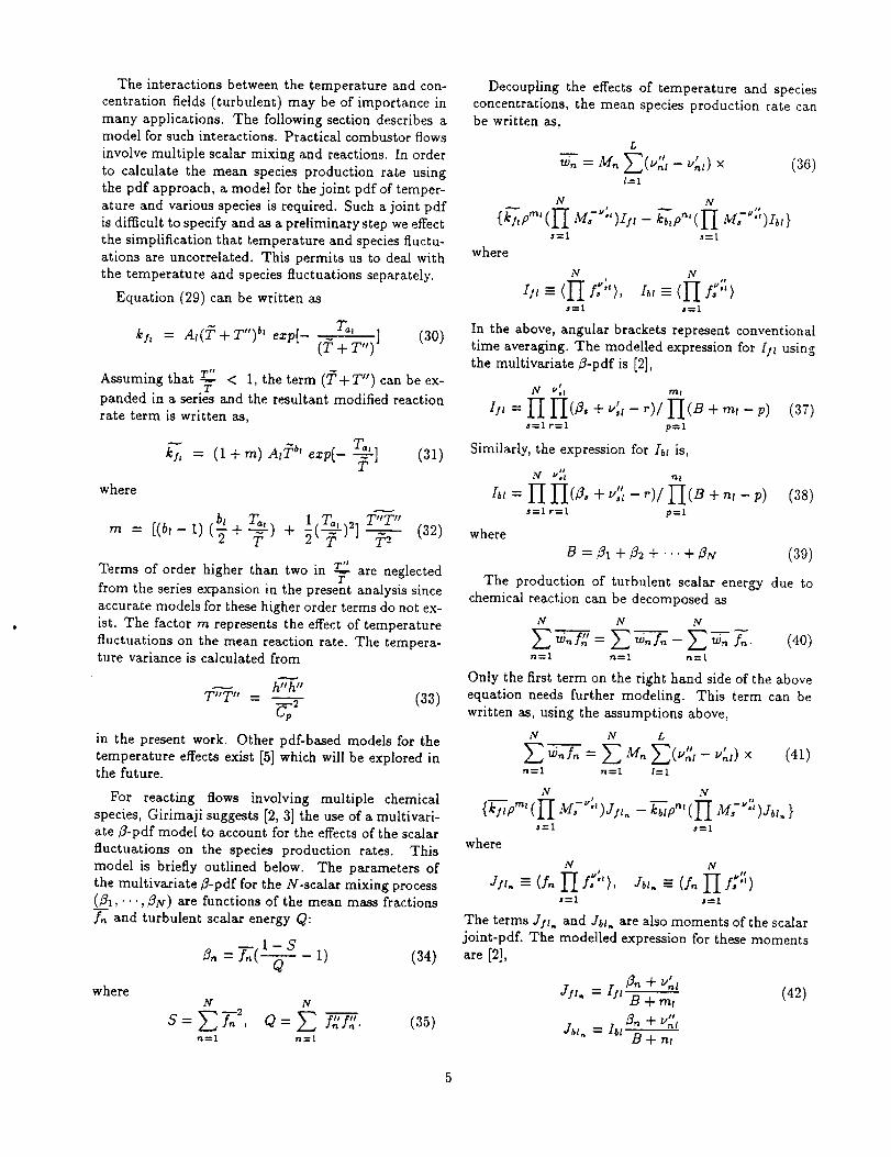
The interactions between the temperature and con-

centration fields (turbulent) may be of importance in

many applications. The following section describes a

model for such interactions. Practical combustor flows

involve multiple scalar mixing and reactions. In order

to calculate the mean species production rate using

the pdf approach, a model for the joint pdf of temper-

ature and various species is required. Such a joint pdf

is difficult to specify and as a preliminary step we effect

the simplification that temperature and species fluctu-

ations are uncorrelated. This permits us to deal with

the temperature and species fluctuations separately.

Equation (29) can be written as

kf, = At(_' + T") b' ezp[- (_ + T,)] (30)

Assuming that T"---- < 1, the term (T+T") can be ex-T

panded in a series and the resultant modified reaction

rate term is written as,

kl"_, = (1 + m) At:_ b_ ex.p[- Ta,.-_-] (31)

where

bl Ta,. i T_, )_ T"T"m = [(b,-i)(7+ -}-)+ _(-_-] f,. (32)

Terms of order higher than two in T"---- are neglectedT

from the series expansion in the present analysis since

accurate models for these higher order terms do not ex-

ist. The factor m represents the effect of temperature

fluctuations on the mean reaction rate. The tempera-

ture variance is calculated from

T,_T,, h'_,= _ (33)

in the present work. Other pdf-based models for the

temperature effects exist [5] which will be explored inthe future.

For reacting flows involving multiple chemical

species, Girimaji suggests [2, 3] the use of a multivari-

ate 8-pdf model to account for the effects of the scalar

fluctuations on the species production rates. This

model is briefly outlined below. The parameters of

the multivariate 8-pdf for the N-scalar mixing process

(81," • ", 8N) are functions of the mean mass fractions

f,_ and turbulent scalar energy Q:

8,=_(1_3 I) (34)

whereN N

s= r o= (35)r_=l n=1

Decoupling the effects of temperature and species

concentrations, the mean species production rate can

be written as,

L

'/)_: Mr Z_.,< at - i%l) x (36)I----1

N N

{gPm'( H M:V"')I;t- ;¢bZpa'(H MZ"")Ia,}

s=1 s----I

where

N N

b,--<l--Is::'>,_,- <l-Is;;">s=l s=l

In the above, angular brackets represent conventional

time averaging. The modelled expression for/'fz using

the multivariate 8-pdf is [2],

t

b,= I-Il-I(_.+ 4,- ,)II]:(B+ m,_ p) (ans----I r----i p=l

Similarly, the expression for Ibl is,

is1_tr b'sl _l

a,= I-[_(Z.+d_-,)/_(B+_,-p) (3s)s----1 r=l p----I

where

B = 81 + 8._ + -" + 8_¢ (39)

The production of turbulent scalar energy due to

chemical reaction can be decomposed as

N N N

woJ"= w./o- F.. (40)n=l n=l n=l

Only the firstterm on the right hand side of the above

equation needs further modeling. This term can be

written as, using the assumptions above,

N N L

_"{I/' -- 'Z w'_f'_ -" Z M, A.._' "' u,_,)x (41)

n=l n=l I=i

N N

{Vp_" (rI M;':, )jr,. -_r,(rI M;<,)j_,. }s=l s=l

where

N N

h,. = (A I-Iff:'>.J_,. = (AlI/::")s=l s=l

The terms Jlt_ and Jbl. are also moments of the scalar

joint-pdf. The modelled expression for these moments

are [2],

JI',, - b' ,6. + _'_l (42)B+mt

nl

B+n_

Substitution of equation (42) into equation (41) leadsto the model for the source/sink of turbulent scalar

energy. The main advantage of this choice of the

assumed-pdf model is that the chemistry related mod-

els are obtained analytically and no numerical inter-

gration in the species space is necessary.

The turbulence-thermochemistry interaction models

require the enthalpy variance and the turbulent scalar

energy distributions. The modeled equations for en-

thalpy variance (h'h t') and turbulent scalar energy(Q)are of a form similar to that of the turbulent kinetic

energy:

+ Ox I - 2pu_'G" Oz i 2fie_

+ b 7 jC( + + +. (43)

For g = h"h', G = h, ffJ=0, _r = Pr and o'g = Pr_.

v "_ t,,';7-,7,,G=.f,,,+= _,,__tw,,/_,o.=Forg = L_n=ljnjn, 2 N • ,!

Sc and _g = Set. The dissipation term in the aboveequation is assumed to be

eg --- Cg kg -- CgC2wg (44)

The model for _---n=IV'N_'_J,;';'r'', is given in equations (40)-(42). The constants C_ are assigned a value of 0.5.

Solution of the modeled governing equations

The equations are discretized and integrated in

space and time to obtain steady state solutions using

an elliptic solver SPARK [13]. The governing equa-tions are written in vector form as follows.

bU b_ i

_- + Oz--7 = H (45)

where U is the vector of dependent variables, _i areflux vectors containing convective and diffusive terms

(repeated indices indicate summation), and H is the

source vector containing production/dissipation terms.

The temporally discrete form of equation (45) is

u "+1 = u" - _xt [0+;' _ H.+I ] (46)0z i

where n is the old time level and n + 1 is the new timelevel.

The source terms in the k- and w-equations are de-

coupled by suitable manipulation of the w term in the

present analysis in order to alleviate the computationalstiffness introduced by these terms. For example, in

the k-equation, the dissipation term is written as,

C_.fiwk = C2fik _" (47)

The term w* is taken from the most recent calcula-

tion step. The source terms of the w-equation arealso manipulated in a similar manner. These nonlin-

ear turbulence source terms are treated in a pointwise-implicit manner while solving the turbulence equations

by rewriting equation (46) as,

(I OH 0+ 7- At_U) (r-r "÷I - u") = - At [-_- - H"] (48)

The discretized equations are solved by means of afourth-order compact scheme.

RESULTS AND DISCUSSION

Choosing a flow configuration to demonstrate the ef-

fect of turbulence-chemistry interactions is a difficult

task due to the lack of guidelines based on prior data(experimental or otherwise). Since the present work

is part of a larger task of establishing a solution pro-

cedure for high speed propulsion systems (scramjets),the initial choice fell on a two-dimensional high speed

reacting mixing layer. Non-reacting and reacting high

speed mixing layers have already been computed us-

ing the computational procedure described above [14].Available experimental data were used to validate the

prediction procedure. The fl-pdf model to account forthe effect of species concentration fluctuations on the

mean production rate of species was also introduced in

conjunction with the k- e turbulence model before [1].The main aim of the present work is to introduce the

results obtained by coupling the fl-pdf model with an

improved version of the k- w model [6].

A schematic of the flow problem is given in Figure 1.

The two streams are, air (U =1606 m/see, T =1600 K

with fH2=0.0, fo==0.267 and fN2=0.733) and hy-

drogen (U =1250 m/see, T =254 K with fH_=l.O,

fo_=0.0 and fY2=O.O). The two streams are super-sonic with the air stream Mach number of 2.07 and

hydrogen stream Mach number of 1.03. The inlet mean

velocity is assumed to have a hyperbolic tangent pro-file, thus imitating the flow that exists downstream of

the splitter plate trailing edge. A constant turbulence

intensity level is used in the free stream for arriving

at the initial distribution of turbulent kinetic energy

and the specific dissipation rate. The pressures are

matched between the two streams (P =1 atm.). A 13-

step, 8-species H2 - Air reaction model (Table 1) hasbeen used for the finite-rate chemistry system consid-ered here. A 101 X 81 grid (101 points in flow direc-

tion, 81 points in the transverse direction) was usedfor the calculations. The length of the flow domain

is 0.25 m and its width is 0.05 m. In all the figuresshown in this report, y refers to the lateral distance

measured from the outer edge of the lower stream. Thetitle g refers to calculations that include the interac-tion model.

6

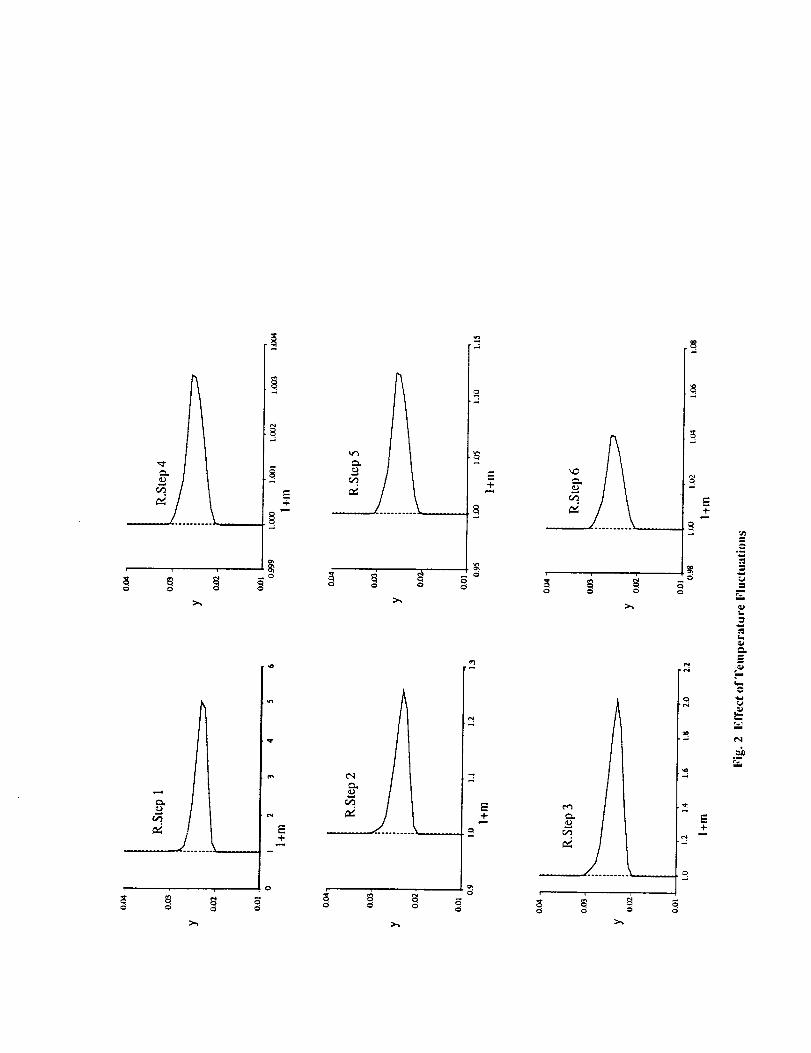
Asa first step,thedifferencemadeby thetemper-aturefluctuationsmodel(28) isexplored.Figure2showsthefactor(1+ m) as a function of y for repre-sentative reaction steps at the exit plane of the flow

domain. The need for including the temperature fluc-

tuations is evident in the figure. The forward reac-

tion rate changes by as much as 400 percent (reaction

step 1) due to the effect of this model. The speciesproduction rate is a strong function of the reaction

rate (32) and hence will be affected by the inclusionof this model.

The effect of the turbulence-chemistry interactions

model on the species production rate is shown in the

next few figures. Figure 3 shows the production rates

of the major species involved (H2, O,., H20, OH)

as functions of y at the exit plane. Computational

results obtained with (k-w-g) and without (k-w) the

effect of these interactions are shown in the figure. Itis seen that the net change in the production rate in

the shear layer/reaction zone is reduced by the effect

of these interactions for the species H2, 02 and H20.For the species OH, the effect of these interactions

seems to be to reverse the rate of production from thecase where the interactions are not included. While

it is not conclusive whether the turbulence-chemistry

interactions increase or decrease the production ratesof individual species, it is important to note that these

interactions do have a significant effect on progress ofthe chemical reactions.

Figures 4 show the distribution of the streamwise

velocity and static temperature as a function of y atthe exit plane. The effect of the interactions seems to

be felt more at the edges of the mixing layer/reaction

zone than anywhere else. In the Going back to fig-ure 3, the production rate seems to be sensitive to the

temperature gradients rather than the temperature it-

self. Turbulence affects the distribution of tempera-

ture both directly (thermodynamic energy equation)and indirectly (via the shear layer effect). This effectis transmitted through the interactions model and is

seen in the chemical production rate profiles. Figure 5shows the effect of the interactions on the species dis-

tributions. The effect seems to be more pronounced in

the case of the products (H20, OH) than the primaryreactants (Hu, On). The changes are larger in regions

of higher gradients (on the fuel stream side for H2 and

air stream side for 02, for example).

One of the unknown yet crucial factors associated

with the present work is the lack of prior knowledgeas to the effect of turbulence on chemical reactions

and the reverse effect of the chemical reactons (heat

release, concentration change) on the turbulent field.Which of these effects is dominant is a debatable is-

sue. Based on the results shown in this report as well

as other similar computations (not shown) carried outby the author, it is not possible to come up with a def-

inite answer to this question. It is also not established

whether the type of flow configuration (mixing layer,

jet, boundary layer) has any significance in this dis-

cussion. So far, all computations using the proposed

model have been done for reacting mixing layer (2-D and coaxial jets) involving the mixing and reactionbetween fuel and oxidizer streams. It is not certain

whether a premixed reacting flow configuration willshow a amore pronounced effect of these interactions

than the non-premixed cases studied so far. Also theeffect of the interactions near a solid wall is an area

worth exploring.

An interesting aspect of the analysis is that the par-

ticular turbulence model chosen (k - e as opposed tok -w, for example) seems to have an effect on the

overall predictions [1]. Since the g-equations, whichprovide the variances needed to construct the interac-

tions model, are strongly coupled (via their produc-tion terms) with the turbulence model equations it isalso essential to differentiate between the effects of the

turbulence model and the turbulence-chemistry inter-

action model. This brings up the importance of theaccuracy of the turbulence model which was one of

the main reasons for carrying out this task using the

k-w turbulence model. It is crucial to keep the short-

comings of the model in perspective while attemptingto validate the results. The assumptions made in ar-

riving at the model, such as the decoupling of temper-

ature and concentration effects, are as important asthe model itself in some cases.

On the positive side, this effort represents a signifi-

cant push in the right direction in this very important

area of turbulent reacting flows. The model is simple

to use and is easily adaptable to other types of tur-bulence closures such as the Reynolds stress models.

More improvements can certainly be done in terms of

using more realistic models for the temperature andconcentration fluctuations such as a pdf-based model

for temperature effects (as opposed to the moment

model employed here), a joint-pdf model to representthe effects of both the temperature and the concen-

tration fields etc. However, in order for the model to

be useful for practical applications, it must be kept in

a form which promotes ease of use as well as compu-tational economy. This is the main reason for resort-

ing to a two-equation level turbulence model in thepresent work. A concerted validation effort is crucial

to ensure the success of the modelling efforts. Onedebilitating factor in this regard is the nonexistence

of useful experimental data. It is extremely difficult,

if not almost impossible, to obtain such experimen-

tal data using present day equipment. An alternative

seems to be direct numerical simulations (DNS) which

hasshownpromisingsignsin relativelysimplerflow

configurations. Inspite of the major advances madein the area of DNS in recent years, it still is a devel-

oping field and is far from providing useful data for

validation purposes in cases such as the present work.

CONCLUSIONS

A turbulence-chemistry interaction model has beenproposed in conjunction with a recent version of the

two-equation k- w model of turbulence for use in

chemically reacting flows. Preliminary computationscarried out with the model for the case of a two-

dimesional, high speed, reacting mixing layer indicatethat these interactions have a significant effect on the

flow predictions. The species production rates of in-

dividual species seem to be affected by these interac-

tions. It is not possible, yet, to quantify the effectsof these interactions based on available data. More

detailed analysis of the various aspects of the model

developmental process need to be done.

ACKNOWLEDGMENTS

[6]

[7]

[8]

[9]

[lO]

[11]

This work was supported by the Applied Computa-

tional Fluids Branch of the Fluid Dynamics Division

at NASA Ames Research Center under Cooperative [12]agreement number NCC 2-715. The author would like

to acknowledge the valuable role played by Dr.S.S. Gir-imaji of ICASE, NASA Langley Research Center in the [13]development of the model.

References [14]

[1] Narayan, J. R. and Girimaji, S. S., "Tur-

bulent Reacting Flow Computations IncludingTurbulence-Chemistry Interactions." AIAA-92-0342, 1992.

[2] Girimaji, S. S., "A Simple Recipe for Mod- [15]

cling Reaction-rates in Flows with Turbulent-

Combustion", AIAA-91-1792, 1991.

[3] Girimaji, S. S., "Assumed 13-pdf model for turbu-

lent mixing: Validation and Extension to MultipleScalar Mixing", Combustion Science 8J Technol-

ogy, Vol.78, 1991, pp 177-196.[16]

[4] Pope, S. B., "Computations of Turbulent Com-

bustion: Progress and Challenges", Proc. 23rd

Symposium (Int.) on Combustion, The combus-

tion Institute, Pittsburgh, PA, 1990, pp 591-612.

[5] Frankel, S.H., Drummond, J.P. and Hassan,

H.A., "A Hybrid Reynolds Averaged/pall Clo- [18]sure Model for Supersonic "I_urbulent Combus-tion", AIAA-90-1573, 1990.

Wilcox, D.C., "A Two-Equation Turbulence

Model for Wall-Bounded and Free-Shear Flows",AIAA Paper 93-2905, 1993.

Mentor, F. R., "Zonal Two Equation k-_,. Tur-

bulence Models for Aerodynamic Flows", AIAAPaper 93-2906, 1993.

Sarkar, S., Erlebacher, G., Hussaini, M. Y., and

Kreiss, FI. O., "The Analysis and Modeling of

Dilatational Terms in Compressible Turbulence",NASA CR 181959, 1989.

Jones, W.P. and Launder, B.E., "The Prediction

of Laminarization with a Two-Equation Model of

Turbulence", Int. J. Heat Mass Transfer, Vol.15,

1972, pp 301-314.

Zeman, O., "Compressible Turbulence Subjected

to Shear and Rapid Compression", Eighth Sym-posium on Turbulent Shear Flows, Munich, Ger-many, 1991.

Narayan, J. R., "A Two-Equation Turbulence

Model for Compressible Reacting Flows." AIAA-91-0755, 1991.

Wilcox, D.C., "Progress in Hypersonic Turbu-lence Modeling", AIAA-91-1785, 1991.

Carpenter, M. H., "Three-Dimensional Computa-tions of Cross-Flow Injection and Combustion in

a Supersonic Flow", AIAA-89-1870, 1989.

Narayan, J. R., Sekar, B., "Computation of Tur-

bulent High Speed Mixing Layers Using a Two-

Equation Turbulence Model." Proceedings of theCFD Symposium on Aeropropulsion, NASA Lewis

Research Center, Cleveland, Ohio, April 24-26,1990.

Drummond, J. P., Carpenter, M. H. and Riggins,D. W., "Mixing and Mixing Enhancement in Su-

personic Reacting Flows", High Speed Propulsion

Systems: Contributions to Thermodynamic Anal-ysis, ed. E. T. Curran and S. N. B. Murthy, Amer-

ican Institute of Astronautics and Aeronautics,Washington, D. C., 1990.

Drummond, J. P.,"A Two-Dimensional Numeri-

cal Simulation of a Supersonic, Chemically Re-

acting ML'dng Layer", NASA TM 4055, 1988.

[17] "Free Turbulent Shear Flows", NASA SP-321,

Vol.1, 1972.

Brown, G. L. and Roshko, A., "On Density Effects

and Large Structure in Turbulent Mixing Layers",]. Fluid Mech., vol. 64, pt. 4, 1974, pp. 775-816.

[19]Papamoschou,D. andRoshko,A., "The Com-pressibleTurbulentShearLayer: An Experi-mentalStudy", J.Fluid Mechanics, v.197, 1988,

pp 453-477.

[20] "Seventh Symposium on Turbulent Shear Flows",Vol.1 and 2, Stanford University, Stanford, Cali-

fornia, 1989.

[21] Oldenborg, 1%.et al., "Hypersonic Combustion Ki-netics - Status Report of the Rate Constant Com-

mittee, NASP High-Speed Propulsion TechnologyTeam", NASA TM 1107, 1990.

[22] Williams, F. A., Combustion Theory. Addison-

Wesley Publishing Company, Inc., Reading, MA,pp. 358-429, 1965.

[23] Favre, A., "Statistical Equations of Turbulent

Gases", Ins_itut de Mechanique Siatis_ique de laTurbulence, Marseille.

Table 1. H2 - Air Reaction System

No. Reaction

1 H+O2=O+OH

2 OH + H2 _---H20 + H

3 O+H2=OH+H

4 OH+ OH ---H_O + 0

5 H+OH+M=H20+M

6 H+H+M_H2+M

7 O+O+M,=O2+M8 H+O+M=OH+M

9 H+O2+M=HO2+M

I0 OH + H02 = H_O + 02

II H + H O_ = H_ + 02

12 H + H02 = OH +OH

13 0 + H02 = OH + O_

14 H02 + H02 _- H202 + 02

15 H + H_O_ = H2 + H02

16 OH + H_02 = H20 + H02

17 H + H20_ = H20 + OH

18 0 + H_02 = H02 + OH

19 OH + OH + M _- H202 + M

20 OH + OH _ H__ + 02

Species : H2, 02, H20, OH, H, O, HOz, H202 and

N_(inert)

M is a third body (all species included)

U

Air_-....-H 2 ---

Fig. 1 Mixing Layer. schematic

cD

-T-

°jo

Ln

-.,4

o

_ _ _ _°

E4-

_t

#

°°o _

_L

r_

f!-T-

,,o

E÷

v_°_

_J

i

t..

Tu

imu

_o

3_

3_

ss

_3

_ o

c_

©

©

LI

°_

L

&=_ °_

qm _'_ °__b

°_

",0

II

E-

_ 3

i

t_...i

im

=

f._

.4 ._

"s

33

f'3 3

c_

_o

c5

c_

i

3_

I

3 _

©

rj}

o__o

u

o_

_N

APPENDIX- B

AIAA-94-Z313

Computation Of High Speed TurbulentReacting Flows Relevent To Scramjet

Combusters

Johnny Narayan and Gregory MolvikMCAT Institute

Moffett Field, California

and

G.WadawadigiUniversity of Texas at ArlingtonArlington, Texas

COMPUTATION OF HIGH-SPEED TURBULENT REACTING FLOWS RELEVANT TO

SCRAM JET COMBUSTORS

J.R. Narayan"

MCAT Institute, Moffett Field, CA.

G. Wadawadigi?

U. of Texas at Arlington, Arlington , Texas.

and

G. Molvik t

MCAT Institute, Moffett Field, CA.

ABSTRACT

Computations are done on flow configurations thatresemble the reaction zone in the scramjet combus-

tor flows. Compressible, reacting, turbulent flow so-

lutions are obtained. A two equation (k-e) modelwith compressibility correction is used to calculate the

flow field. A finite rate (8-species, 13-reaction steps)chemistry model for hydrogen-air combustion has been

used. Computations are carried out using the Navier-

Stokes solver TUFF. Predictions are compared withavailable experimental data and also those obtained

by using the code UPS.

NOMENCLATURE

A,b

C1,C_.,C.E

f.H

h

k

]¢f ,kb

L

Mn

M,N

Pr,Pr_

PSc,SctT

T=t

0

coefficients in Arrhenius rate equationturbulence model constants

total internal energymass fraction of species n

total enthalpy

static enthalpy

turbulent kinetic energyforward and backward reaction rate constants

number of reaction steps

Molecular weight of species nTurbulent Mach number

number of chemical specieslaminar and turbulent Prandtl numbers

pressurelaminar and turbulent Schmidt numbers

temperature

Activation Temperaturetime

velocity vector

production rate of species nstreamwise coordinate

* Senior Research Scientist, Senior Member AIAA.

t PostDoctorla Fellow, Member AIAA.

*'Senior Research Scientist, Member AIAA.

zjY

61iff

%

rl

7

V

PO"k , 0"_

rii

Subscriptst

j_h coordinatetransverse coordinate

Kronecker delta

turbulence energy dissipation ratecompressible dissipation rate

compressibility correction coefficient

ratio of specific heats

specific dissipation rate

laminar viscosityturbulent viscosity

kinematic viscositydensityturbulence model constants

stress tensor

flux vector in j,h direction

turbulent quantity

INTRODUCTION

Hypersonic travel requires propulsion systems whichare different from the conventional ones used in most

of the modern aircraft. The supersonic combustion

ramjet (scramjet) is a system considered to be suit-

able for high speed applications. There has been a

tremendous amount of activity in the area of scramjet

research in recent years ( [1]- [11]). Some of the re-lated topics include inlet configuration, mbdng layers,

mixing enhancement, combustor configuration, finiterate chemistry models and chemical kinetics. The fuel

used in the scramjet varies depending upon the ap-

plication. For example, hypersonic waveriders using

hydrocarbon fuels have been designed [12] for applica-tions in the moderate hypersonic speed regimes. For

Mach numbers of the order of 15 and above, hydro-

gen is generally considered to be the fuel of choice.

In the present work, hydrogen is the fuel used in thecomputations.

The present work represents a computational el-

fort inestablishingasolution procedure for _hypersonicpropulsion applications. The entire task of establish-

ing the solutions procedure must then be divided into

smaller tasks dealing with subsets such as turbulence

modelling, chemical kinetics, geometry etc. One such

task is the topic for the present study. Here, the rele-

vant flow features of the combustor, namely the mixingand chemical reaction between the fuel and oxidizer

streams, is addressed. The flow field in a scramjet is

complex. It is turbulent and compressible involvinghigh heat release. The solution procedure should ad-

dress all aspects of the flow field adequately. It should

be capable of accurately modelling the turbulent field,

taking into account the effects of compressibility, andaddressing the changes associated with heat release.

Also, the interactions between the distinct physicalaspects of the flow such as the effect of heat release

on turbulence, the interaction between turbulence and

chemistry etc. must be properly addressed. Signifi-

cant progress has been made in addressing these areas

via accurate and realistic modelling in recent years [6].

Remarkable advances have been made in the area

of turbulence modelling, accounting for a variety of

factors that affect the flow field. Compressibility cor-

rection models to account for the effects of compress-ibility, near-wall turbulence models to deal with the

transition from fully turbulent to zero turbulence, vis-

cous dominated flow field near no-slip boundaries andmodifications to models to account for flow curvature

are some examples. A wide variety of turbulence mod-

els, including algebraic (zero-equation), one-equation,

two-equation, Reynolds stress and large eddy simula-

tion models, are available (for example references [13] -[15]) depending upon the sophistication and accuracy

desired and the limits imposed by numerical solutionprocedures.

Thermodynamic and chemical kinetic models [16]

applicable to the scramjet flows have been undergoingcontinuous improvements in recent years. Accuratemodelling of thermodynamic variables as functions of

temperature which are valid over a wide range of tem-peratures is an example. In flows such as the oneassociated with the scramjet, the time scales associ-

ated with fluid dynamics and chemical reaction (not tomention the turbulence scales) require that the com-bustion process be modelled via a finite rate chem-istry mechanism. Such a mechanism should account

not only for the major species (reactants and prod-ucts) involved in the chemical reactions but also the

intermediate transient ones which play a vital role inthe reaction progress process. Accurate models for the

chemical reactions in the scramjet combustor, thus, is

a crucial aspect of the solution procedure.

The design of the combustor is strongly dependent

upon factors such as the mixing between fuel and ox-idizer streams, presence of shocks in the flow field,

boundary layer effects, flow separation, extent of chem-ical reaction within the combustor and so on. The nu-

merical solution procedure should have the capability

of addressing all of these factors while maintaining the

required accuracy and robustness. There is a glut ofuseful numerical solvers applicable for a wide variety

of flows including all speed regimes. Computational

algorithms which are fast and accurate are being im-proved everyday.

Even though there are a wide variety of sophisti-cated and physically accurate thermodynamic, chem-ical kinetic and turbulence models available it is not

always possible to use the most accurate and elabo-rate versions in a numerical simulation due to the lim-

itations imposed by computer memory requirements,

computational economy, ease of use and adaptability

to practical problems. Solutions often are required,

especially in ihe engineering industry which is the end

user for such solvers, in a short time using comput-

ers that may not be the fastest available. As a result,

compromises must be struck between physical accu-

racy and computational feasibility and it is this aspectwhich differentiates between various solvers that exist

today.

In the present study, an attempt is made to es-

tablish a solution procedure for scramjet combustor

flow predictions from the perspective of the discus-

sion above. The models chosen to represent the tur-

bulent and chemistry fields reflect the compromise be-

tween physical accuracy and computational economymentioned above. The code chosen for the computa-

tions is the TUFF [17] code and the solutions are com-

pared with those obtained with the UPS [18, 20] code.The turbulence model chosen is the two-equation k - eturbulence model with low Reynolds number modifi-

cations [13]. However, the Baldwin-Lomax algebraic

model is also available as an option. The compress-ibility effects are included via the compressibility cor-

rection model proposed by Zeman [19]. The fuel used

is hydrogen although the numerical solver can easily

be modified for hydrocarbon fuels. A 9-species, 20-

reaction steps chemical kinetics model for hydrogen-air combustion [16] is available. For the computations

presented in this report, an abbreviated version (8-species, 13-steps) of this model has been used.

Mixing plays a major role in high speed combus-

tor flows. The reaction zone is mainly confined to

mixing layers that exist between fuel and oxidizer

streams. Two flow configurations are chosen for thestudy. The first is the well known Burrows-Kurkov

experiment [21] in which hydrogen and vitiated air

streams (two-dimensional) mL_ and react. The second

easeis that of anaxisymmetricconfiguration[22,23]wheretwocoaxialjets (fuelandoxidizer)mixandre-act. Experimentaldatafrom compressible,reactingmixinglayersisstill scarcewhichhindersthevalida-tionof thecalculationprocedure.Theavailabledatafromtheabovetwoexperimentsareusedto comparewith the predictions.Thegoverningandsecondaryequationsusedin thecomputationshaveallbeende-scribedin detailin thereferencescitedabove.Onlyanabreviatedequationsetwillbegivenin thepresentpa-per.Thecomputationswereperformedonthesuper-computersof NASandNASAAmesResearchCenter(C-90).

GOVERNING EQUATIONS

The equations used for computations are described

in detail in references [6, 7, 10] and [24]. Only the

forms of the modelled equations used in the present

study are given here. Density-weighted averaging isused to derive the mean flow equations from the in-

stantaneous coservation equations. The dependent

variables, with the exception of density and pressure,are written as

¢ = ¢ + ¢" (I)

where the ¢" is the fluctuating component of the vari-• able under consideration and its Favre-mean ¢ is de-fined as

_-_(2)

In this equation, the overbar indicates conventional

time-averaging. Density and pressure are split in theconventional sense as,

p = _ + p' and p = _ + p' (3)

The averaged continuity and momentum equations are

_- + 0_ - 0 (4)

o_u, _u, ujT + oz i -

where

_,_ = _¢_-- +ozj

o_, a_s + _ (5)

-_x_)bus" 32 cgxkcgu_6ii (6)

with repeated indices indicating summation.

In the two-equation turbulence model, the two tur-

bulence variables are the turbulent kinetic energy (k)and the dissipation rate (e) [13] defined as

k - pu_'u_'2_ (7)

and

0U.'l 0t_zn

= (8)

Boussinesq approximation is used to obtain closure

of the averaged equations. Here the Reynolds stresstensor is written as,

. /"_"'_ 2pui us = -_ Sis - "_"#k6#

OU_ OUs 20U_ ,hiO:ci + Ozi 30zk (9)

turbulent/eddy viscosity defined as

k 2

#, = G#-- (1o)

with Cu=0.09.

The modelled momentum equation, then, is,

O-_U_ _r_u_uj _Y_ 20_k

o--T + O_ - az_ + 3 az---T6_so

- a_:7[ (# + _,) s,] (11)

The effects of compressibility are included via the

model proposed by Zemaa [19]. Here, the compress-ible dissipation terms are expressed as functions of the

turbulent kinetic energy dissipation rate and the local

turbulent Mach number. The compressibility effects

are represented by a component of the dissipation rate(¢e) given as

¢, = Kce

K_ = ,TF(M,)

2kM, = a_ (12)

where a is the local speed of sound and F(Mt) is a

function of the local turbulent Mach number (Mr).F(Mt) is given by

= 1_ezp[_(Mt.o),],--M, M, > MtoF(M,)

= O, M_<M_o

with M,0=0.1 and 7/=0.75. The modelled turbulent

kinetic energy equation is [6, 13]

a#_ op_usa--i- + Ozs -- P_ - fie(1 + K¢)

+ _. [(_ + G _._.]#, ) a_ (13)

.

where

---- -- pu i uj(14)

The modelled e-equation used (no compressibility

corrections) in the present analysis [13] is given below.

0 fi_) 0¢.+ + 7, 1 (is)

where P_ is the production term in the turbulent

kinetic energy equation. The model constants used

in the analysis are C1-1.44, 6"2=1.92, _r,=l.0,_=1.3, Pr=0.72, Pr,=l.0, Sc=0.22and Set=l.0.

The mass-averaged total energy can be written in

terms of the total enthalpy as

P (16)

The correlations between the fluctuating velocity and

the scalar fluctuations are modelled using a gradient-diffusion hypothesis..4 typical model is of the form

- = A o86r, (_zi) (17)

where _r_sis a coefficient which, normally, is a constant.

For ¢ = fa (n represents the species) , _r_ = Sc,, and

for the static enthalpy, (_ = h), o'¢ = Prt. Using the

above definition, and omitting the body force contri-

bution, the time-averaged and modelled energy equa-tion [6] is

o [ f, f,, ) o'_ f,,) ok 18

where _rk comes from the turbulent kinetic energyequation. The modeled species continuity equation is

__ 0+ - TM (19)

The modelled form of the mean species production

rate due to chemical reaction (w"_n)is given, for a finite-

rate system involving L reaction steps and N species,in the following general form:

UJr_

L

Z( It iM. v._ - v,.) x (20)I----1

N , N

s=l s ,_----i

where

N N

ml=Z ' Z "I/M, nl -- !./._I

' and " are the number of molecules of thewhere, u_t u_t

scalar s involved in the/-th reaction step in the forwardand backward directions, respectively. The forward

and backward rate-constants of the reaction l are givenby k/_ and k_t respectively.

k/_ = A_T _' ezp[ T_t.---f-] (21)

where A_, bt and Ta_ are numerical constants specificto the given reaction step I. k_ is determined from the

equilibrium constant for the/-th reaction step and kit.

Solution of the modeled equations

The equations are discretized and integrated in

space and time to obtain steady state solutions using

the finite-volume based numerical solver TUFF [17].The TUFF code contains many desirable features for

the computation of three-dimensional, hypersonic flow

fields. It has non-equilibrium, equilibrium and perfect

gas capabilities along with an incompressible option.It employs a finite-volume philosophy to ensure that

the schemes are fully conservative. The upwind in-

viscid fluxes are obtained by employing a new tem-

poral lZiemann solver that fully accounts for the gasmodel used. This property allows the flow field dis-continuities such as shocks and contact surfaces to be

captured by the numerical scheme without smearing.Total Variation Diminishing (TVD) techniques are in-

cluded to allow extension of the schemes to higher or-

ders of accuracy without introducing spurious oscilla-

tions. The schemes employ a strong coupling betweenthe fluid dynamic and species conservation equations

and are made fully implicit to eliminate the step-size

restriction of explicit schemes. This is necessary since

step-sizes in a viscous, chemically reacting calculationcan be excessively small for an explicit scheme, and

the resulting computer times prohibitively large. A

fully conservative zonal scheme has been implemented

to allow solutions of very complex problems. The

schemes are made implicit by fully linearizing all of

the fluxes and source terms and by employing a mod-ified Newton iteration to eliminate any linearization

and approximate factorization errors that might oc-

cur. Approximate factorization is then employed toavoid solving many enormous banded matrices. As

mentioned before, the options for turbulence models

include both zero and two equation models (both k - eand k - _). For more details about the solution pro-cedure the reader is directed to the reference cited

above [1]].

RESULTS AND DISCUSSION

Two reacting flow configurations have been chosen

for the present study. As mentioned before, the Navier

Stokes solver TUFF has been used for the computa-

tions. The first one is the case of coaxial jets [22, 23]

where a hydrogen jet flows (inner jet) coaxially with

an outer vitiated air (mass fractions: oxygen=0.246,water=0.209 and nitrogen=0.545) jet. A schematic of

the flow problem is given in Figure 1. The two streams

are, air (U=1380 m/sec, T=l180 K with p=107000N/m2) and hydrogen (U=1774 m/sec, T=545 K with

p=112000 N/m2)., The air stream is supersonic with a

Mach number of 1.97 and the hydrogen stream Mach

number is 1.00. The inlet mean velocity is assumed

to have a step profile with the two jets having uni-form speeds at the specified values (no experimental

data available). The velocity in the lip region of the

inner jet tube wall (finite wall thickness) is assumedto be zero. The inlet temperature profile is derived

based on the experimental data given for a location

just downstream of it (shown later). The inlet speciesmass fraction distributions are also chosen based on

the experimental data provided at the same down-

stream location. A constant turbulence intensity level

is used in the free stream for arriving at the initialdistribution of turbulent kinetic energy and the dis-

sipation rate. A 13-step, 8-species H2- Air reactionmodel (Table 1) has been used for the finite-rate chem-

istry system considered here. A 81 X 91 grid (81 points

in flow direction, 91 points in the radial direction) wasused for the calculations. The inner jet/tube diameter

(D=0.00236 m) is used as a reference length. The to-tal length of the flow domain is equal to 43.1 D. The

outer boundary (radial) of the flow domain is taken to

be at y=17 D. A more detailed description of the flow

parameters is given in Table 2. The region outside thelimits of the air jet is assumed to be still air at a tem-

perature of 273 K. The two-equation (k-e) turbulencemodel is used along with the finite rate H2-Air chem-

istry model mentioned above. In all the figures shownin this report, y refers to the radial distance measured

• from the axis of the coaxial system of jets.

Figures 2 - 3 show the results of the computations.Figure 2 shows the computed and experimental distri-

butions of species mole fractions. The figure is de-signed in a two-column format. The left side col-

umn represents the inlet (first x-location) data and

the right side column is the data at the exit plane

(z/D=43.1 D). As seen in these figures, the inlet

data agreement between the computations and exper-

iment is not perfect, especially around the jet edges,and this might affect the computed distributions at

downstream locations. The comparison between pre-dictions and experiment at the downstream location

(z/D=43.1 D) is good given the above mismatch be-

tween the two data at the inlet. The development

of the reaction zone after ignition is not predictedwell. The experimental data indicates that the reac-

tion zone (depicted by the water mole fraction distri-

bution) spreads more quickly than the predictions in-dicate. The predictions show the reaction zone to be

off-center whereas the experimental data shows the re-

cation zone to be closer to the axis of symmetry. How-

ever, there is very good qualitative agreement between

the data with the peak values of the reaction prod-ucts predicted very well. The flow domain was seen

to have a wave-like structure as shown by the pre-

dicted profiles. The worst agreement seems to be for

the case of oxygen. However, when the initial pro-files of oxygen are compared one finds that there too

is the worst agreement between computations and ex-

periment which may be reason for the problem down-stream. Figure 3 shows the comparison of static tem-

perature data. The agreement between predictions

and experiment is good qualitatively displaying similartrends. The uncertainty associated with the accuracyof the experimental data is unknown. There are con-

siderable differences between the data presented by the

two references [22, 23], especially in the temperature

profiles. Overall, there is good qualitative agreementbetween the predictions and experiment.

The second test case considered is the Burrows-

Kurkov experiment [21]. The flow configuration is two-

dimensional. A schematic diagram of the configuration

is given in figure 4. No-slip walls bound both the upperand lower regions (y=0 and y=yma_). The lower wall

is inclined to form an expansion surface. Hydrogen isinjected along this surface into a vitiated air stream.The two streams mix and react downstream of the

injection location (inlet). The hydrogen stream is in-

jected at a velocity of 1216 m/sec and a temperatureof 254 K. The airstream comes in at a speed of 1764m/sec and a temperature of 1270 K. Full details about

the flow parameters and geometry are given in Table 3.

In this case, the reference length used in the hydrogen

jet width at inlet, h (h=0.004 m). The models for tur-bulence and chemistry are identical to the ones used

for the coaxial jet case. The grid size is 81 X 121

(81 grid points in the axial (z) direction and 121 grid

points in the transverse direction). The total length

of the solution domain is 0.356 m (z/h=89). Avail-

able inlet data have been used for the first-plane pro-files which improved the predictions remarkably over

the solutions obtained with uniform profiles. The so-

lutions are compared with the available experimental

data at this location (exit) in figures 5-7. The solu-

tions carried out with the space marching PNS codeUPS [20] using the Baldwin-Lomax turbulence model

are also given for comparison.

Figure5 showsthe compariosnbetweenthe pre-dicteddistributionsof thespeciesmolefractionsandthe correspondingexperimentaldata. As seeninthesefigures,thereisexcellentagreementbetweentheTUFFpredictionsandexperiment.ThepredictionsbytheUPScodedonotagreeverywellbutstill thereisverygoodqualitativeagreementwiththeexperimentaldata.Figure6 comparesthepredictedprofilesof exitplanetotal temperatureandMuchnumberwith the [1]experimentaldata. Thereis goodqualitativeagree-mentin thecaseoftemperatureandverygoodoverallagreementin thecaseof theMuchnumberdistribu-tion.Figure7showsthecomparisonbetweenthepre- [2]dictionsandexperimentof the lowerwall (hydrogenjet side)pressure.Ignitioncausesthepressureriseintheprofile. Ignitionseemsto bedelayedin thecaseofthepredictionsaccompaniedbyamorepronounced [3]pressurerise.

Highspeedreactingflowssuchasthetwocasesstud-iedherearecomplexinspiteof their simplegeome-tries. The interactionsbetweenthedifferentaspects [4]of theflowsuchasturbulence,chemicalkinetics,heatreleaseetc. areverydifficultto understandand,toa largeextent,impossibleto modelaccurately.Mod-erndayexperimentalfacilitiesstill cannotmakecom-pletemeasurementsin suchflows.Onlymeanvalues [5]of temperature,velocity,pressure,speciesconcentra-tionsetc. areavailable,if any. Eventhen,the un-certaintiesassociatedwith thedataforceoneto ac-ceptthemonlywithcertainreservations.Given that, [6]there is almost never a chance for perfect agreement

between predictions and experiment in all the areas.

While the advances made in measurement techniquesimprove every day, the fruits of these advancements

(ie. accurate measurements) are not realized imme- [7]

diately. As a result, today's computations will have

only old data for validation (in the present case, the

best data is already four years old) purposes which iscertainly the case here. Unless more accurate experi- [8]

mental data with minimum uncertainties are available,

the best a computational effort can hope for, in terms

of validation, is probably what is seen here. [9]

CONCLUSIONS

Computation of the flow fields of two high-speed, [10]turbulent, reacting flow configurations involving finite-rate chemical kinetics for hydrogen-air combustion

have been carried out. A two-equation (k - e) turbu-lence model with compressibility corrections has been

used. The predictions are compared with available

experimental data. Good qualitative agreement is

present between computations and experiment. Moredetailed experimental data is necessary. [11]

ACKNOWLEDGMENTS

This work was supported by the Applied Computa-tional Fluids Branch of the Fluid Dynamics Division at

NASA Ames Research Center under the Cooperativeagreement number NCC 2-715.

References

Marvin, J. G., "A CFD Validation Roadmap ForHypersonic Flows", NASA Technical Memoran-

dum 103935, 1992.

Ebrahimi, H. B., "CFD Validation For ScramjetCombustor and Nozzle Flows, Part I", AIAA-93-1840, 1993.

Vitt, P. H., Riggins, D. W. and McClinton, C.R., "The Validation and Application of Numeri-

cal Modelling to Supersonic Mixing and ReactingFlows", AIAA-92-0626, 1992.

Pdggins, D. W. and McClinton, C. R., "A Com-

putational Investigation of Mixing and React-ing Flows in Supersonic Combustors", AIAA-92-

0626, 1992.

Eklund, D. R. and Northam, G. B., "A Numeri-

cal Study of the Effects of Geometry on the Per-formance of a Supersonic Combustor." AIAA-92-0624, 1992.

Narayan, J. R. and Girimaji, S. S., "Tur-

bulent Reacting Flow Computations IncludingTurbulence-Chemistry Interactions." AIAA-92-0342, 1992.

Narayan, J. R., "A Two-Equation Turbulence

Model for Compressible Reacting Flows." AIAA-91-0755, 1991.

Eklund, D. R., "Calculation of Supersonic Tur-bulent Reacting Coaxial Jets." AIAA Journal,

Vol.28, No.9, 1990, pp 1633-1641.

Carpenter, M. H., "Three-Dimensional Computa-

tions of Cross-Flow Injection and Combustion in

a Supersonic Flow", AIAA-89-1870, 1989.

Drummond, J. P., Carpenter, M. I=I. and Riggins,

D. W., "MLxing and MLxing Enhancement in Su-

personic Reacting Flows", High Speed PropulsionSystems: Contributions to Thermodynamic Anal-

ysis, ed. E. T. Curran and S. N. B. Murthy, Amer-

ican Institute of Astronautics and Aeronautics,

Washington, D. C., 1990.

Drummond, J. P.,"A Two-Dimensional Numeri-

cal Simulation of a Supersonic, Chemically Re-

acting Mixing Layer", NASA TM 4055, 1988.

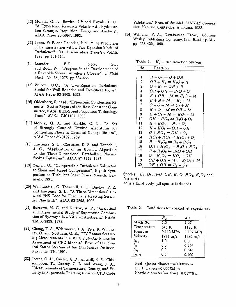
[12]Molvik, G. A. Bowles,J.V.andHuynh,L. C.,"A HypersonicResearchVehiclewithHydrocar-bonScramjetPropulsion:DesignandAnalysis",AIAA Paper93-5097,1993.

[13]Jones,W.P.andLaunder,B.E.,"ThePredictionof Laminarization with a Two-Equation Model of

Turbulence", Int. J. Heat Mass Transfer, Vol.15,1972, pp 301-314.

[14] Launder, B.E., Reece, G.J.

and Rodi, W., "Progress in the Development of

a Reynolds Stress Turbulence Closure", J. FluidMech., Vol.68, 1975, pp 537-566.

[15] Wilcox, D.C., "A Two-Equation Turbulence

Model for Wall-Bounded and Free-Shear Flows",AIAA Paper 93-2905, 1993.

[16] Oldenborg, R. et al., "Hypersonic Combustion Ki-

netics - Status Report of the Rate Constant Com-

mittee, NASP High-Speed Propulsion TechnologyTeam", NASA TM 1107, 1990.

[17] Molvik, G. A. and Merkle, C. L., "A Set

of Strongly Coupled Upwind Algorithms for

Computing Flows in Chemical Nonequilibrium",AIAA Paper 89-0199, 1989.

[18] Lawrence, S. L., Chaussee, D. S. and Tannehill,

J. C., "Application of an Upwind Algorithmto the Three-Dimensional Parabolized Navier-

Stokes Equations", AIAA 87-1112, 1987.

[19] Zeman, O., "Compressible Turbulence Subjected

to Shear and Rapid Compression", Eighth Sym-posium on Turbulent Shear Flows, Munich, Ger-many, 1991.

[20] Wadawadigi, G. Tannehill, J. C., Buelow, P. E.

and Lawrence, S. L., "A Three-Dimensional Up-

wind PNS Code for Chemically Reacting Scram-jet Flowfields", AIAA 92-2898, 1992.

[21] Burrows, M. C. and Kurkov, A. P., "Analytical

and Experimental Study of Supersonic Combus-tion of Hydrogen in a Vitiated Airstream." NASA

TM X-2828, 1973.

[22] Cheng, T. S., Wehrmeyer, J. A., Pitz, R. W., Jar-

ret, O. and Northam, G. B., "UV Raman Scatter-

ing Measurements in a Mach 2 H2-Air Flame forAssessment of CFD Models." Proc. of the Cen-

tral States Meeting of the Combustion Institute,Nashville, TN, 1991.

[23] Jarret, O. Jr., Cutler, A. D., Antcliff, R. R., Chit-

somboon, T., Daneey, C. L. and Wang, J. A.,

"Measurements of Temperature, Density, and Ve-

locity in Supersonic Reacting Flow for CFD Code

Validation." Proc. of the 25th JANNAF Combus-

tion Meeting, Huntsville, Alabama, 1988.

[24] Williams, F. A., Combustion Theory. Addison-

Wesley Publishing Company, Inc., Reading, MA,pp. 358-429, 1965.

Table 1. H2 -- Air Reaction System

No. Reaction

1 H+O2,-_-O+OH

2 OH + H2 = H20 + H

3 O+H_=OH+H

4 OH+ OH = H20 + 0

5 H+OH+Mr"---H20+M

6 H+H+M=_-H2+M

7 O+O+M,_--O2+M8 H+O+M._-OH+M

9 H+O2+Mr'---HO2+M

10 OH + HO_ _ H20 + 0211 H + HO_ _-- H2 + 02

12 H + H02 _ OH + OH

13 0 + H02 _ OH + 02

14 H 02 + H 02 = H202 + 02

15 H + H202 = H2 + H02

16 OH + H202 _ H20 + H0217 H + H20_ = H20 + OH

18 0 + H202 _- H02 + OH

19 OH + OH + M ,_- H202 + M

20 OH + OH = H2 + 02

Species : H2, 02, H20, OH, H, O, HO_., H202 andN2(inert)

M is a third body (all species included)

Table 2. Conditions for coaxial jet experiment

H2 AirMach No. 1.0 1.97

Temperature 545 K 1180 KPressure 0.112 MPa 0.107 MPa

Velocity 1774 m/s 1380 m/sfH2 1.0 0.0

fo2 0.0 0.246

fN, 0.0 0.545fH_o 0.0 0.209

Fuel injector diameter=0.00236 m

Lip thickness=0.000725 m

Nozzle diameter(air flow)=0.01778 m

Table3. ConditionsforBurrows-KurkovExperiment

H2 AirMach No. 1.0 2.44

Temperature 254 K 1270 KPressure 0.1 MPa 0.1 MPa

Velocity 1216 m/s 1764 m/s

fI_ 1.0 0.0fo, 0.0 0.258

fN, 0.0 0.486

fH_o 0.0 0.256

Fuel injector height=0.004 m

Duct height at inlet=0.0938 m

Duct height at exit=0.1048 m

I I---" H2

Uai r --- 1380 m/s Tai r = 1180 K Pair = 107000 N/m 2

UH2 = 1774 m/s TH2 = 545 K PH2= 112000 N/m 2

Fig. 1 Coaxial jet case : schematic

I.

aJ

o

m

Z

, ,o

I-

r

J •

o

I •

©

o

o

I.

:-_o

o _ _

I-

o

o

I-

Z

e I 0

.=

r_

I!

r_

)<

t_O0

IIr_

I.,.J

.'/

_p

Lrl

I" o

,CIoF,

i-.

0,

=4,)

0,

_S

v.

_-- ._-_r_

,-' C_

It U

C_I

II II

I°°

L.

L.

r_

I

a _ 0

o_

fT. °

I ! "

_ _ o oq

©

v.I

o

II

_ o

C_

z

o

li •

4

c_ aa g'_

0

r"

C_

C_

°°

t-

O

t4r_

I-

c__C

C_

II

i

o

L.

L

t_

Q,

[-i,

@

t...

!

@t_.L.

_ .

i _-. _

IIi-.

_ _ _ _ o,I) c_

c_

II

tu

_L

_4

°o

L.

L,t.,

r"

_L

APPENDIX- C

AIAA-94-2948j_ / J

/ r

Prediction Of Turbulent Reacting FlowsRelated To Hypersonic Airbreathing

Propulsion Systems

Johnny NarayanMCAT InstituteMoffett FieldCalifornia

PREDICTION OF TURBULENT REACTING FLOWS RELATED TO HYPERSONIC

AIRBREATHING PROPULSION SYSTEMS

J.R. Narayan °

MCAT Institute, Moffett Field, CA.

ABSTRACT 0

Computation of scramjet combustor flows is the z

main thrust of this work. Computations are done on xiflow configurations that resemble the reaction zone in Y

the scramjet combustors. Compressible, reacting, tur- _,_"

bulent flow solutions are obtained. A two equation o_0,o_(k-e) model with compressibility correction is used to cd, _,,

calculate the flow field. A finite rate (9-species, 20- 61i

reaction steps) chemistry model for hydrogen-air com- ebustion has been used. Computations are carried out _c

using the Navier-Stokes solver TUFF. Predictions are _?

compared with available experimental data and also 7

those obtained by using the codes UPS and SPARK.A turbulence-chemistry interaction model is included. #

This model represents the first step in the effort to in- Pt

clude these interactions in high-speed reacting flows, vA two-dimensional reacting mixing layer has been used Pfor demonstration, o'k, o'_

r_j

NOMENCLATURE

A,b

Cl,C:,C.Cs,C6E

f.gH

h

k

kl ,kbL

M_

M,N

Pr,Pr_

PRc,ReTR_ ,tL,Sc,SctT

T_t

coefficients in Arrhenius rate equationturbulence model constants

turbulence model constants

total internal energy

mass fraction of species n

scalar variance (enthalpy, mass fraction)total enthalpy

static enthalpy

turbulent kinetic energyforward and backward reaction rate constants

number of reaction steps

Molecular weight of species nTurbulent Mach number

number of chemical specieslaminar and turbulent Prandtl numbers

pressureturbulence model coefficients

turbulence model coefficients

laminar and turbulent Schmidt numbers

temperature

Activation Temperaturetime

*Senior Research Scientist, Senior Member AIAA.

velocity vector

production rate of species nstreamwise coordinate

jth coordinatetransverse coordinate

turbulence model coefficientsturbulence model coefficients

turbulence model constants

Kronecker delta

turbulence energy dissipation rate

compressible dissipation rate

compressibility correction coefficient

ratio of specific heatsspecific dissipation rate

laminar viscosity

turbulent viscosity

kinematic viscosity

densityturbulence model constants

stress tensor

Subscripts

t turbulent quantity

INTRODUCTION

Propulsion systems for hypersonic applications are

required to use the supersonic combustion ramjet(scramjet) due to the flight regime involved. Due to

the advent of the National Aerospace Plane (NASP)proposed over a decade ago, there has been a consider-

able amount of effort directed at developing a scram-jet based propulsion system for a number of years.

Even though interest in the NASP is waning at presentdue to various reasons, the research effort in the area

of high speed propulsion systems such as the scram-

jet still is going strong as evidenced by the enormous

number of reports published in the literature and na-

tional and international meetings. It is not within thescope of the present report to list and describe all the

work going on in the area of high speed propulsion.

However, references [1] to [11] are some examples ofthe vast amount of work in this area. The area of

high speed propulsion, especially for hypersonic appli-

cations, is a complex one encompassing a wide vari-

ety of related topics such as inlet configuration, mix-

ing layers,mixingenhancement,combustorconfigu-ration,finite ratechemistrymodelsandchemicalki-netics.Bothhydrocarbonsandhydrogenareconsid-eredasfuelsdependingupontheapplication.Forex-ample,hypersonicwaveridersusinghydrocarbonfuelshavebeendesigned[1]forapplicationsin themoderatehypersonicspeedregimes.ForMachnumbersof theorderof15andabove,hydrogenisgenerallyconsideredto bethefuelofchoice.Thepresentworkrepresentsacomputationaleffortin establishinga solutionproce-dureforhighspeedpropulsioningeneralandscramjetflowsinparicular.

The flow field in a scramjetis complex. It isturbulentand compressibleinvolvinghigh heatre-lease.Thesolutionprocedureshouldaddressall as-pectsof theflow field adequately.It shouldbeca-pableofaccuratelymodellingtheturbulentfield,tak-ingintoaccounttheeffectsof compressibility,addressthechangesassociatedwith heat release and accuar-

rely describe the chemical kinetics mechanism which

is vital in high speed combustion. Also, the inter-actions between the distinct physical aspects of theflow such as the effect of heat release on turbulence,

the interaction between turbulence and chemistry etc.

must be properly addressed. Progress has been made

in addressing these areas via accurate and realistic

modelling in recent years [6]. However, a significantamount of work remains to be done before any real-istic claims for accurate models in these areas can be

made. There have been remarkable advances made

in the area of turbulence modelling, accounting fora variety of factors that affect the flow field. Com-

pressibility correction models to account for the ef-

fects of compressibility, near-wall turbulence modelsto deal with the transition from fully turbulent to zero

turbulence, viscous dominated flow field near no-slipboundaries and modifications to models to account for

flow curvature are some examples. A wide variety of

turbulence models, ranging from the algebraic (zero-

equation) models to Reynolds stress and large eddy

simulation models are available (references [12]= [14]

are some examples) depending upon the sophistica-tion and accuracy desired and the limits imposed by

numerical solution procedures.

Thermodynamic and chemical kinetic models [15,

16] applicable to the scramjet flows have been under-

going continuous improvements in recent years. Ac-curate modelling of thermodynamic variables as func-

tions of temperature which are valid over a wide range

of temperatures is an example. The design of the com-

bustor is strongly dependent upon factors such as the

mixing between fuel and oxidizer streams, presence of

shocks in the flow field, boundary layer effects, flow

separation, extent of chemical reaction within the com-

bustor and so on. The numerical solution procedure

should have the capability of addressing all of thesefactors while maintaining the required accuracy and

robustness. Computational algorithms which are fast

and accurate are being improved everyday and beingadapted in present day numerical solvers applicable for

a wide variety of flows including all speed regimes. In-

spite of the existence of a wide variety of sophisticatedand physically accurate models in many of the areas

associated with high speed propulsion, it is not always

possible to use the best models in a numerical sim-

ulation due to the limitations imposed by computerresources, computational economy and adaptability to

practical problems. Fast turnaround is a key factor

in the success of any solver in practical problem solv-

ing situations. Compromises must be struck between

physical accuracy and computational feasibility.

The present work represents the effort made to es-

tablish a solution procedure for high speed propulsion

related flows. The models chosen to represent theturbulent and chemistry fields reflect the compromise

between physical accuracy and computational econ-

omy mentioned above. The code chosen for the com-

putations are the TUFF [17] code and the SPARK

code [6, 9]. The solutions are compared with those ob-

tained with the UPS [18, 19] code and available exper-imental data. The turbulence model chosen is the two-

equation (k - e) turbulence model with low Reynolds

number modifications [12]. The compressibility effectsare included via the compressibility correction model

proposed by Zeman [20]. The fuel used is hydrogen and

a 9-species, 20-reaction steps chemical kinetics model

for hydrogen-air combustion [15] (Table 1) is used (inits abbreviated version).

In the present task, major emphasis is on the turbu-

lence model(s) used for reacting, compressible flows.

Specifically, the interaction between the turbulencefield and the chemical kinetics is of interest. The effect

of turbulence on phenomena such as mixing betweentwo streams, boundary layer etc. has been studied ex-

tensively and it is an ongoing process. However, there

is not enough work done in the area of turbulence-

chemistry interactions in order to either emphasize or

neglect the importance of such interactions. The mainreason for this is the fact that it is extremely difficult to

quantify these interactions experimentally. There have

been efforts aimed at establishing pdf-based models for

coupling the turbulence field with the thermochemi-

cai fieldin numerical simulations. References [6], [21]

and [22] are just a few of the many reports availablein this area. There has also been a concerted effort to

generate validation data bases through direct numeri-

cal simulations which is still in its early stages.

In the present work, on the thermochemistry front,

the effects of temperature and species the effects of

temperatureandspeciesfluctuationsaredecoupled.Forthetemperature-turbulenceinteraction,amomentmodelis used[6]. Thechemicalspeciesfluctationsareaccountedforusinganassumedmultivariate-fl-pdfmodel[6, 21,22].Thethermochemistrymodelsusedhereareindependentof themodelfor theturbulentvelocityfield. Thesemodelsrequirethe solutionoftheevolutionequationsfor allthemeanflowthermo-chemicalvariables,turbulencevariables(k andeitherw or e), enthalpy variance and turbulent scalar energy 0"_Ui

(sum of all the species variances). The CFD code used Ot

is SPARK [9]. where

Mixing plays a major role in high speed combustor

flows. The reaction zone is mainly confined to mixinglayers that exist between fuel and oxidizer streams.

Efficient mixing of fuel and oxidizer is very impor-

tant for the design of combustor size. Mixing lay-ers ranging from subsonic to supersonic speeds have

been studied extensively over the years. In the present

work, a two-dimensional and axisymmetric compress-

ible, reacting, mixing layer (hydrogen-air) is computedwith the aforementioned codes. Experimental data

from compressible, reacting mixing layers is still scarce

which hinders the validation of the calculation pro-cedure. Three flow configurations are chosen for the

study. The first two are chosen to demonstrate the

solution procedure without the turbulence-chemistryinteraction model and the last case is used exclu-

sively to demonstrate the effect of this model. The

first case is the well known Burrows-Kurkov experi-ment [23] in which hydrogen and vitiated air streams

(two-dimensional) mix and react. The second case is

that of an axisymmetric configuration [24, 25] where

two coaxial jets (fuel and oxidizer) mix and react. The

two-equation, (k-e) turbulence model is used for theseapplications. Available data from the above two ex-

periments are used to compare with the predictions.

The last case considered is a two-dimensional, react-ing, mixing layer problem. Here, the two-equation, where

(k-w) turbulence model [14] has been used. The gov-

erning and secondary equations used in the computa-tions have all been described in detail in the references

cited above. Only an abreviated equation set will be

given in the present paper. The computations were

performed on the supereomputers of NAS and NASAAmes Research Center.

GOVERNING EQUATIONS

The equations used for computations are described

in detail in references [6, 7, 10] and [26]. Only the

forms of the modelled equations used in the present

study are given here. Density-weighted averaging isused to derive the mean flow equations from the in-

stantaneous coservation equations. In the following,

a tilde represents Favre (density-weighted) averagingand a simple overbar represents conventional time

averaging. The averaged continuity and momentumequations are

0-7 + 0z_ = 0 (1)

_u_ ui _ Opui uj 0_-_+ Ozi - Oz_ Oz_ + _ (2)

2 0u_ &_ (3)3 0z_

with repeated indices indicating summation.

In the two-equation turbulence model, the two tur-

bulence variables are the turbulent kinetic energy (k)

and either the dissipation rate e [12] or the specific dis-sipation rate w [14]. The definitions of these variables

can be found in the cited references. Boussinesq ap-

proximation is used to obtain closure of the averagedequations. The Reynolds stress tensor is written as,

2

Ou_ OUj 20UkSij = _ + Ozi 3 Ozk _<i

(4)

where/_t is the turbulent/eddy viscosity defined as

]¢2d, = C.5--

6(5)

with C_,=0.09, or, with w defined as,

(6)

(/:_eT )49 _ +', RoC5 =

100 1+_ R° J(7)

with R¢=6 and

_kRe T = ---:_

wp(s)

/_t is given as

_r, = _-Z_Ld

(9)

with

{:]¢_R_

I+K_:R,.

(10)

and

3=_=c6/3, R_=8, c6=_ (11)

The modelled momentum equation, then, is,

0

- a_---T[ (# + #') s,j (12)

The effects of compressibility are included via the

model proposed by Zeman [20]. Here, the compress-

ible dissipation terms are expressed as functions of the

turbulent kinetic energy dissipation rate and the localturbulent Mach number. The compressibility effects

are represented by a component of the dissipation rate

(e_) given as

ec = Kce

K_ = rlF(Ms)2k

M, = a--"7 (13)

where a is the local speed of sound and F(Ms) is a

function of the local turbulent Mach number (Mr).

F(Mt) is given by

A/L

F(lVlt) = 1- ezp[-(M*_._"'°)e], Ms _M, o

= 0, Mt < Mto (14)

with Mso=0.1 and 0=0.75.

kinetic energy equation is [6, 12]

The modelled turbulent

O#k O#kUy+ - Pk - #_,(1+ Ko)

Ot cgzi

O #s) ak,+ _-_C(_+ _ _-_J (15)

where _ is either e or wk and

OU_ (16)P_ = _ p_;,u_,_T_j

The modelled e-equation used (no compressibilitycorrections) in the present analysis [12] is given below.

O#e O#eUy"-_ + Ozj

6

= (G Pk-C2Ze)

a #, ) at .+ b-_j[(#+ 7, b_l (171

where P_ is the production term in the turbulent ki-

netic energy equation. The modelled w-equation [14]

is given below.

Or" + Ozj

where

and

a} P_- C6_ 2+ _£ D_W

a #,) ae+ b-_jC(z+ _ _] (18)

Ok c3_

Dk,_ = (3zj Oz I (19)

1 a0+ -_-z=c, - n_ (20)

2a* 1+ R--_R_

The turbulence constants are c_0=0.1, /_:2.2,_=1.67, Ct=1.44, C__=1.92, _r_=l.0, _r_=l.3,

Pr=0.72, Prr=l.0, Sc=0.22 and Sc_=l.0. and

o'd = 0.0, D_,<0

= 0.3, D_ >0

The mass-averaged total energy can be written in

terms of the total enthalpy as

_=_ P (21)

The correlations between the fluctuating velocity and

the scalar fluctuations are modelled using a gradient-diffusion hypothesis. A typical model is of the form

,,,, #, o_)- _,,__ = -- (-_-- (22)¢7Z_

where o'_ is a coefficient which, normally, is a constant.

For ¢ = fn (n represents the species) , _¢_ =Sct, andfor the static enthalpy, (¢ = h), o'_ = Prt. Using the

above definition, and omitting the body force contri-

bution, the time-averaged and modelled energy equa-tion [6] is

It It .

Ot + a_ - Ox---_.(_'_ - _ _ - pu, u¢ )u_

+ _ _+_ T;7_+(_+_ _I_31

where _r_ comes from the turbulent kinetic energyequation. The modeled species continuity equation is

+ -- _bn - "W:-'_] (24)c,zi

The modelled form of the mean species production

rate due to chemical reaction (_b,_) is given, for a finite-rate system involving L reaction steps and N species,

in thefollowinggeneralform:L

_"lu" ' (25)uL_ = M,_/__,t ,_l - v,_l) x

{kl,p",._._-:-.-k,,o"'I-I( )""},

where

N N

Z' E"rnl -- lgsl, rll --" Psi

s=l s=l

where, v_t and v_ are the number of molecules of thescalar s involved in the l-th reaction step in the forwardand backward directions, respectively. The forward

and backward rate-constants of the reaction I are given

by kit and kbl respectively.

klt = ArT _'' ezp[ T_tl---_-j (26)

where At, bt and Ta, are numerical constants specificto the given reaction step I. kbl is determined from the

equilibrium constant for the/-th reaction step and kit.

Turbulence-chemistry interaction model

Practical combustor flows involve multiple scalarmixing and reactions. In order to calculate the mean

species production rate using the probability density

function (pdf) approach, a model for the joint pdf of

temperature and various species is required. Such a

joint pdf is difficult to specify and as a preliminarystep we effect the simplification that temperature and

species fluctuations are uncorrelated. This permits us

to deal with the temperature and species fluctuations

separately. Equation (26) can be written as

To,_ ] (27/ki, = At(T + T") b' ezp[- (_ + T")

Assuming that T" (_< 1, the term +T") can be ex-T

panded in a series and the resultant modified reaction

rate term is written as,

k]-'_ = (1 + m) A,T b' ezp[- T_,--_-I (281

where

b_ Ta,. I Ta, 2 T"T"

rn= [(b,-I)(_-+ -_--)+ _(T) ] _ (29)

Terms of order higher than two in T"--_ are neglectedT

from the series expansion in the present analysis since

accurate models for these higher order terms do not

exist. The factor rn represents the effect of tempera-ture fluctuations on the mean reaction rate. The tem-

perature variance is calculated from the enthalpy vari-ance [6].

For reacting flows involving multiple chemicalspecies, a multivariate _-pdf model is used to ac-count for the effects of the scalar fluctuations on the

species production rates [6]. Relevant features of this

model are briefly outlined below. The parameters of

the multivariate _-pdf for the N-scalar mixing process

(ill,'", fiN) are functions of the mean mass fractionsm

f,_ and turbulent scalar energy Q:

where

--- I) (30)

N N

s= ]_E2, Q= _/z/z. (3_)n=l n:l

Decoupling the effects of temperature and species

concentrations, the mean species production rate canbe written as,

L--r- _-'_¢v" 'wn - Mn A.._ nt - v,zl) x (32)

l---I

N N

{'_hpm'(H M;-":')II,_ kb"_pm(H M;"ld;)Ib,}$=I $=i

where

N N

#,- <I-I/5,>,r,, = <II.f::_>s=i s=l

In the above, angular brackets represent conventional

time averaging. The modelled expression for I/r using

the multivariate _-pdf is [21],

N v',_ rnE

Ij,= HH(il, +v:,-r)/H(B-Fmt-p ) (33)J:l r:l p=l

Similarly, the expression for [bt is,

Ibl = HH(19, +v'i-rl/H(B+nt-p) (34)$:I r:l p¼l

where

B = #t +f12 +...+#iv (35)

The production of turbulent scalar energy due tochemical reaction can be decomposed as

N N N

= wo/o-E T.. (36)n=l n=l rt:[

Only the first term on the right hand side of the

above equation needs further modeling and details

can be found in reference [6]. The turbulence-

thermochemistry interaction models require the en-

thaipy variance and the turbulent scalar energy distri-

butions. The modeled equations for enthalpy variance

(h"h") and turbulent scalar energy(Q) are of a form

similar to that of the turbulent kinetic energy:

ozg azg 0--Y + 0xi - _ 2/_e9

+ [(g + + fi (37)

For g = h"h", G = h, fi=0, o" = Pr and era = Prt.Iv _, Jv

For g -- _-_,=1 G " "fg f_:, Y.,fi== 2_.=1 w./:_, _ =Sc and u9 = Sct. The dissipation term in the aboveequation is assumed to be

eg = Cg_g = C_Czwg (38)

Solution of the modeled equations

The equations are discretized and integrated in

space and time to obtain steady state solutions us-ing either the finite-volume based numerical solver

TUFF [17] (for the first two test cases) or the fi-

nite difference solver SPARK [9] (for the last case).The TUFF code contains many desirable features for

the computation of three-dimensional, hypersonic flow

fields. It has non-equilibrium, equilibrium and perfect

gas capabilities along with an incompressible option.It employs a finite-volume philosophy to ensure that

the schemes are fully conservative. The upwind in-

viscid fluxes are obtained by employing a new tem-

poral Riemann solver that fully accounts for the gasmodel used. This property allows the flow field dis-continuities such as shocks and contact surfaces to be

captured by the numerical scheme without smearing.Total Variation Diminishing (TVD) techniques are in-

cluded to allow extension of the schemes to higher or-ders of accuracy without introducing spurious oscilla-

tions. The schemes employ a strong coupling between

the fluid dynamic and species conservation equations

and are made fully implicit to eliminate the step-sizerestriction of explicit schemes. This is necessary since

step-sizes in a viscous, chemically reacting calculation

can be excessively small for an explicit scheme, and

the resulting computer times prohibitively large. Afully conservative zonal scheme has been implemented

to allow solutions of very complex problems. The

schemes are made implicit by fully linearizing all of

the fluxes and source terms and by employing a mod-ified Newton iteration to eliminate any linearization

and approximate factorization errors that might oc-

cur. Approximate factorization is then employed to

avoid solving many enormous banded matrices. As

mentioned before, the options for turbulence models

include both zero and two equation models (both k -e

and k - w). For more details about the solution pro-cedure the reader is directed to the reference cited

above [17]. The SPARK solver is a finite difference el-

liptic solver using a hybrid McCormack scheme. More

details about the solution procedure can be found in

references [6] and [9].

RESULTS AND DISCUSSION

The computational effort is divided into two parts.The first part deals with the demonstration and valida-

tion process for the solution procedure by application

to high speed turbulent reacting flows involving finite

rate hydrogen-air chemistry. As mentioned before, theNavier Stokes solver TUFF has been used for the com-

putations. Two reacting flow configurations have beenchosen for this part. The first test case considered is

the Burrows-Kurkov experiment [23]. The flow con-

figuration is two-dimensional. A schematic diagram of

the configuration is given in figure 1. No-slip walls

bound both the upper and lower regions (y=O and

y--yrna_). The lower wall is inclined to form an expan-sion surface. Hydrogen is injected into a vitiated airstream. The two streams mix and react downstream of

the injection location (inlet). The hydrogen stream is

injected at a velocity of 1216 m/see and a temperatureof 254 K. The airstream comes in at a speed of 1764m/sec and a temperature of 1270 K. Full details about

the flow parameters and geometry are given in Table 2.

In this case, the reference length used in the hydrogenjet width at inlet, h (h=0.004 m). A constant turbu-

lence intensity level is used for arriving at the initial

distribution of turbulent kinetic energy and the dis-sipation rate. A 13-step, 8-species H_. - Air reaction

model (Table 1) has been used for the finite-rate chem-

istry system considered here. The grid size is 81 X 121

(81 grid points in the axial (z) direction and 121 grid

points in the transverse direction). The total lengthof the solution domain is 0.356 m (z/h=89). Avail-

able inlet data have been used for the first-plane pro-

files which improved the predictions remarkably overthe solutions obtained with uniform profiles. The so-

lutions are compared with the available experimentaldata at this location (exit) in figures 2-4. The solu-

tions carried out with the space marching PNS codeUPS [19] using the Baldwin-Lomax turbulence model

are also given for comparison.

Figure 2 shows the comparison between the pre-dicted distributions of the species mole fractions andthe corresponding experimental data. As seen in

these figures, there is excellent agreement between the

TUFF predictions and experiment. The predictions by

theUPSandSPARKcodesdonotagree very well butstill there is very good qualitative agreement with the

experimental data. Figure 3 compares the predicted

profiles of exit plane total temperature with the ex-

perimental data. There is good qualitative agreement

here. Figure 4 shows the comparison between the pre-

dictions and experiment of the lower wall (hydrogen jetside) pressure. Ignition causes the pressure rise in the

profile. Ignition seems to be delayed in the case of the

TUFF predictions accompanied by a more pronounced

pressure rise. A point to note here is the fact that the

SPARK, UPS and TUFF codes produced nearly iden-

tical results for nonreacting mixing layers which is not

the case in the present reacting flow simulations.

The second case is that of coaxial jets [24, 25] wherea hydrogen jet flows (inner jet) coaxially with an

outer vitiated air (mass fractions: oxygen=0.246, wa-

ter=0.209 and nitrogen=0.545) jet. A schematic of the

flow problem is given in Figure 5. The two streamsare, air (U=1380 m/sec, T=l180 K with p=107000

N/m2) and hydrogen (U=1774 m/sec, T=545 K with

p=l12000 N/m2)., The air stream is supersonic with a

Much number of 1.97 and the hydrogen stream Muchnumber is 1.00. The inlet mean velocity is assumed to

have a step profile with the two jets having uniformspeeds at the specified values (no experimental data

available). The velocity in the lip region of the innerjet tube wall (finite wall thickness) is assumed to be

zero. The inlet temperature profile is derived based on

the experimental data given for a location just down-

stream of it (shown later). The inlet species mass frac-tion distributions are also chosen based on the exper-imental data provided at the same downstream loca-

tion. The models for turbulence and chemistry areidentical to the ones used for the first test case. A

81 X 91 grid (81 points in flow direction, 91 pointsin the radial direction) was used for the calculations.

The inner jet/tube diameter (D=0.00236 m) is used

as a reference length. The total length of the flow do-

main is equal to 43.1 D. The outer boundary (radial)of the flow domain is taken to be at y=17 D. A more

detailed description of the flow parameters is given in

Table 3. The region outside the limits of the air jet isassumed to be still air at a temperature of 273 K. The

two-equation (k - e) turbulence model is used alongwith the finite rate H2-Air chemistry model mentioned

above. In all the figures shown for this case, y refersto the radial distance measured from the axis of the

coaxial system of jets.

Figures 6 - 7 show the results of the computations.

Figure 6 shows the computed and experimental distri-

• butions of species mole fractions. The figure is de-signed in a two-column format. The left side col-

umn represents the inlet (first x-location) data and

the right side column is the data at the exit plane

(z/D=43.1 D). As seen in these figures, the inlet

data agreement between the computations and exper-

iment is not perfect, especially around the jet edges,and this might affect the computed distributions at

downstream locations. The comparison between pre-dictions and experiment at the downstream location

(_:/D=43.1 D) is good given the above mismatch be-

tween the computational and experimental data at the

inlet. The development of the reaction zone after igni-tion is not predicted well by the TUFF code whereas

the SPARK code fares better. The experimental data

indicates that the reaction zone (depicted by the water

mole fraction distribution) spreads more quickly than

the predictions indicate. There seems to be a discrep-

ancy between the locations of peak reaction activity

between the predictions (off the axis) and the exper-

iment (closer to axis). However, there is very goodqualitative agreement between the data with the peak

values of the reaction products predicted very well.The flow domain was seen to have a wave-like structure

as shown by the predicted profiles. Figure 7 shows the

comparison of static temperature data. The agreementbetween predictions and experiment is good qualita-

tively displaying similar trends. The uncertainty as-

sociated with the accuracy of the experimental datais unknown. There are considerable differences be-

tween the data presented by the two references [24, 25],especially in the temperature profiles. Overall, there

is good qualitative agreement between the predictionsand experiment.

In the second part, the turbulence-chemistry inter-action model is demonstrated using a two-dimensional

mixing layer configuration. A schematic of the flow

problem is given in figure 8. The two streamsare, air (U =1606 m/sec, T =1600 K with

f_z2=0.0, fo2=0.267 and f_¢_=0.733) and hydrogen

(U =1250 m/sec, T =254 K with fH_=l.0, fo_=O.Oand f_2=O.O). The two streams are supersonic with

the air stream Much number of 2.07 and hydrogenstream Much number of 1.03. The inlet mean veloc-

ity is assumed to have a hyperbolic tangent profile. Aconstant turbulence intensity level is used in the free

stream for arriving at the initial distribution of tur-

bulent kinetic energy and the specific dissipation rate.The pressures are matched between the two streams

(P =1 atm.). A 13-step, 8-species H2- Air reaction

model (Table 1) has been used for the finite-rate chem-

istry system considered here. A 101 X 81 grid (101points in flow direction, 81 points in the transverse di-

rection) was used for the calculations. The length ofthe flow domain is 0.25 m and its width is 0.05 m. In

the figures the title g refers to calculations that includethe interaction model.

The difference made by the temperature fluctuations

model is shown in figure 9. Here the factor (1 + m) is

7

plotted as a function of y for the firstthree reaction

steps at the exit plane of the flow domain. The need

for including the temperature fluctuations is evident

in the figure. The forward reaction rate changes byas much as 400 percent (reaction step 1) due to the

effect of this model. The species production rate is a

strong function of the reaction rate (29) and hencewill be affected by the inclusion of this model. The

effect of the turbulence-chemistry interactions model

on the species production rate is shown in the next few

figures. Figure 10 shows the production rates of the

major species involved (H2, 02, H20, OH) as func-tions of y at the exit plane. Computational results

obtained with (k-w-g) and without (k-w) the effect ofthese interactions are shown in the figure. It is seen

that the interaction between turbulence and chemistry

has a significant effect on the net production rate of

chemical species. While it is not conclusive whetherthe turbulence-chemistry interactions increase or de-

crease the production rates of individual species, it

is important to note that these interactions do have

a significant effect on progress of the chemical reac-

tions. Figure 11 shows the effect of the interactions onthe species distributions. The effect seems to be more

pronounced in the case of the products (H20, OH)

than the primary reactants (H2, 02). The changesare larger in regions of higher gradients (on the fuel

stream side for H2 and air stream side for 02, for ex-

ample).

This effort represents a significant push in the right

direction in this very important area of turbulent re-

acting flows. The model is simple to use and is easilyadaptable to other types of turbulence closures such

as the Reynolds stress models. More improvements

can certainly be done in terms of using more realistic

models for the temperature and concentration fluctua-tions such as a pdf-based model for temperature effects

(as opposed to the moment model employed here), ajoint-pdf model to represent the effects of both the

temperature and the concentration fields etc. How-ever, in order for the model to be useful for practical

applications, it must be kept in a form which promotes

ease of use as well as computational economy. This isthe main reason for resorting to a two-equation level

turbulence model in the present work. A concertedvalidation effort is crucial to ensure the success of the

modelling efforts. One debilitating factor in this re-gard is the nonexistence of useful experimental data.

It is extremely difficult, if not almost impossible, to ob-

tain such experimental data using present day equip-meat. An alternative seems to be direct numerical

simulations (DNS) which has shown promising signsin relatively simpler flow configurations.

CONCLUSIONS

A numerical solution procedure applicable to highspeed reacting flows has been demonstrated. In the

first part, computation of the flow fields of two high-speed, turbulent, reacting flow configurations involv-

ing finite-rate chemical kinetics for hydrogen-air com-

bustion have been carried out. A two-equation (k - e)turbulence model with compressibility corrections has

been used. The predictions are compared with avail-

able experimental data. Good qualitative agreement is

present between computations and experiment. Moredetailed experimental data is necessary. In the sec-

ond part, a turbulence-chemistry interaction model isintroduced and its effect is demonstrated via a two-

dimensional turbulent reacting flow problem. The

interactions seem to have a significant effect on the

species production rate. More detailed analysis is nec-

essary.

ACKNOWLEDGMENTS

This work was supported by the Applied Computa-tional Fluids Branch of the Fluid Dynamics Division at

NASA Ames Research Center under the Cooperative

agreement number NCC 2-715. The author wishes to

acknowledge the contributions of Dr.Gregory Molvik

of MCAT Institute, NASA Ames Research Center,

California and Dr. Ganesh Wadawadigi of Univer-

sity of Texas at Arlington, Texas. Also, the invaluable

contribution to the interaction model by Dr. Sharath

Girimaji of ICASE, NASA Langley Research Center is

acknowledged and appreciated.

References

[1] Molvik, G. A. Bowles, J.V.and Huynh, L. C.,

"A Hypersonic Research Vehicle with Hydrocar-

bon Scramjet Propulsion: Design and Analysis",AIAA Paper 93-5097, 1993.

[2] Ebrahimi, H. B., "CFD Validation For ScramjetCombustor and Nozzle Flows, Part I", AIAA-93-

1840, 1993.

[3] Vitt, P. H., Riggins, D. W. and McClinton, C.

R., "The Validation and Application of Numeri-

cal Modelling to Supersonic Mixing and ReactingFlows", AIAA-92-0626, 1992.

[4] Riggins, D. W. and McClinton, C. R., "A Com-

putational Investigation of Mixing and React-

ing Flows in Supersonic Combustors", AIAA-92-0626, 1992.

[5] Eklund, D. R. and Northam, G. B., "A Numeri-cal Study of the Effects of Geometry on the Per-

formance of a Supersonic Combustor." AIAA-92-

0624, 1992.

[6]

[7]

[8]

[9]

[10]

[11]

[12]

[13]

[14]

[15]

'[16]

Narayan, J. R. and Girimaji, S. S., "Tur-

bulent Reacting Flow Computations Including

Turbulence-Chemistry Interactions." AIAA-92-0342, 1992.

[17]

Narayan, J. R., "A Two-Equation Turbulence

Model for Compressible Reacting Flows." AIAA-91-0755, 1991.

Eklund, D. R., "Calculation of Supersonic Tur-

bulent Reacting Coaxial Jets." AIAA Journal,

Vol.28, No.9, 1990, pp 1633-1641.

Carpenter, M. H., "Three-Dimensional Computa-

tions of Cross-Flow Injection and Combustion in

a Supersonic Flow", AIAA-89-1870, 1989.

Drummond, J. P., Carpenter, M. H. and Riggins,

D. W., "Mixing and Mixing Enhancement in Su-personic Reacting Flows", High Speed Propulsion

Systems: Contributions to Thermodynamic Anal-

ysis, ed. E. T. Curran and S. N. B. Murthy, Amer-ican Institute of Astronautics and Aeronautics,

Washington, D. C., 1990.

Drummond, J. P.,"A Two-Dimensional Numeri-

cal Simulation of a Supersonic, Chemically Re-

acting Mixing Layer", NASA TM 4055, 1988.

Jones, W.P. and Launder, B.E., "The Prediction

of Laminarization with a Two-Equation Model of

Turbulence", Int. J. Heat Mass Transfer, Vol.15,1972, pp 301-314.

Launder, B.E., Reece, G.J.

and Rodi, W., "Progress in the Development of

a Reynolds Stress Turbulence Closure", 3". Fluid

Mech., Vol.68, 1975, pp 537-566.

Wilcox, D.C., "A Two-Equation TurbulenceModel for Wall-Bounded and Free-Shear Flows",

AIAA Paper 93-2905, 1993.

Oldenborg, R. et al., "Hypersonic Combustion Ki-

netics - Status Report of the Rate Constant Com-

mittee, NASP High-Speed Propulsion TechnologyTeam", NASA TM 1107, 1990.

Jachimowski, C. J., "An Analytical Study of the

Hydrogen-Air Reaction Mechanism with Applica-tion to Scarmjet Combustion", NASA TP 2791,1988.

Molvik, G. A. and Merkle, C. L., "A Set

of Strongly Coupled Upwind Algorithms for

Computing Flows in Chemical Nonequilibrium",

AIAA Paper 89-0199, 1989.

[18] Lawrence, S. L., Chaussee, D. S. and Tannehill,

J. C., "Application of an Upwind Algorithmto the Three-Dimensional Parabolized Navier-

Stokes Equations", AIAA 87-1112, 1987.

[19] Wadawadigi, G. Tannehill, J. C., Buelow, P. E.

and Lawrence, S. L., "A Three-Dimensional Up-

wind PNS Code for Chemically Reacting Scram-jet Flowfields", AIAA 92-2898, 1992.

[20] Zeman, O., "Compressible Turbulence Subjectedto Shear and Rapid Compression", Eighth Sym-

posium on Turbulent Shear Flows, Munich, Ger-

many, 1991.

[21] Girimaji, S. S., "A Simple Recipe for Mod-

eling Reaction-rates in Flows with Turbulent-Combustion", AIAA-91-1792, 1991.

[22] Girimaji, S. S., "Assumed fl-pdf model for turbu-lent mixing: Validation and Extension to Multiple

Scalar Mixing", Combustion Science _ Technol-

ogy, Vol.78, 1991, pp 177-196.

[23] Burrows, M. C. and Kurkov, A. P., "Analytical

and Experimental Study of Supersonic Combus-

tion of Hydrogen in a Vitiated Airstream." NASATM X-2828, 1973.

[24] Cheng, T. S., Wehrmeyer, J. A., Pitz, R. W., Jar-ret, O. and Northam, G. B., "UV Roman Scatter-

ing Measurements in a Much 2 H2-Air Flame forAssessment of CFD Models." Proc. of the Cen-

tral States Meeting of _he Combustion Institute,

Nashville, TN, 1991.

[25] Jarret, O. Jr., Cutler, A. D., Antcliff, R. R., Chit-somboon, T., Dancey, C. L. and Wang, J. A.,

"Measurements of Temperature, Density, and Ve-

locity in Supersonic Reacting Flow for CFD CodeValidation." Proe. of the 25th JANNAF Combus-

tion Meeting, Huntsville, Alabama, 1988.

[26] Williams, F. A., Combustion Theory. Addison-Wesley Publishing Company, Inc., Reading, MA,

pp. 358-429, 1965.

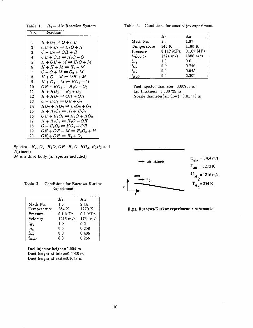
Table 1. H2 - Air Reaction System Table 3. Conditions for coaxial jet experiment

No. Reaction

1 H+O2_O+OH

2 OH+H2_---H20+H3 O+H2-----OH+H

4 OH + OH _ H20 + 0

5 H+OH+M_-_-H20+M

6 H+H+M=H2+M

7 O+O+M_O2+M8 H+O+M_--OH+M

9 H+O2+M_HO2+Mi0 OH + H02 = H20 + 02

ii H + H02 = H2 + 02

12 H + H02 = OH + OH

13 0 + H02 _ OH + 02

14 H 02 + H 02 = H202 + 02

15 H + H202 _- H2 + H02

16 OH+ H202 = H20 + H02

17 H + H202 _- H20 + OH

18 0 + H202 = H02 + OH

19 OH + OH + M = H202 + M

20 0 K+ OH = H2 + 02

Species : H2, 02, H20, OH, H, O, H02, H202 and

N2(inert)

M is a third body (all species included)

Table 2. Conditions for Burrows-Kurkov

Experiment

H2 Air

Mach No. 1.0 2.44

Temperature 254 K 1270 KPressure 0.1 MPa 0.1 MPa

Velocity 1216 m/s 1764 m/s

fH= 1.0 0.0fo_ 0.0 0.258

fN: 0.0 0.486

fargo 0.0 0.256

Fuel injector height=0.004 m

Duct height at inlet=0.0938 m

Duct height at exit=0.1048 m

H2 AirMach No. 1.0 1.97

Temperature 545 K 1180 KPressure 0.112 MPa 0.107 MPa

Velocity 1774 m/s 1380 m/s

fH_ 1.0 0.0fo, 0.0 0.246

fN, 0.0 0.545faqo 0.0 0.209

Fuel injector diameter=0.00236 m

Lip thickness=0.000725 m

Nozzle diameter(air flow)=0.01778 m

Air (vitiated)

i

X

Uai r = 1764 m/s

Tai r = 1270 K

UH2= 1216 m/s

TH = 254 K2

Fig.1 Burrows-Kurkov experiment : schematic

10

I •: J

, i

I '0:

%Z

o

II

! •: o

i

•i ! •

: i

I

i %, • •

t'N

_o

e-

°_

°°

e_

L.t_

u

r=

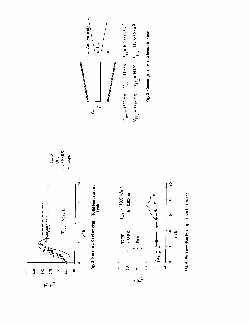
ii ii

.o

._.

m i_

II II

I •: I

oct

C4It

o

o_

°:

_L

e_

"_"

II II

I

41"

$

t--

L--

II

o*

t--

d_

@

!

o

©

?

©

C,

i

III

I'I

e

J

41

iJ

I'

o

oN

l i.

j,

q_

d o _'

Z

l i-

Z

r.

,.

m

m

-&°_

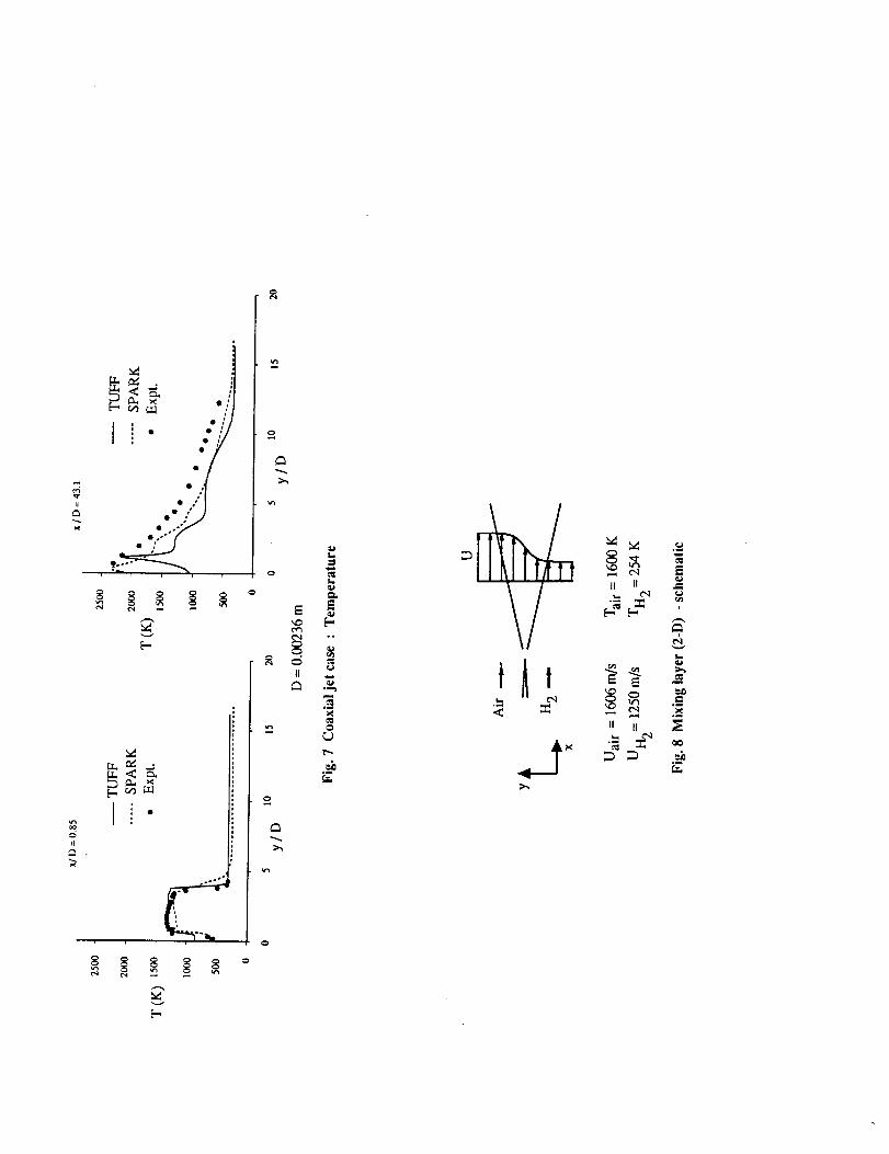
II

lio

_d

E-

CJ

L

f.,

II

r_

_At

o_

II II _--

o_ _

___ ,

_ _ o_

II II _

• _ _1_

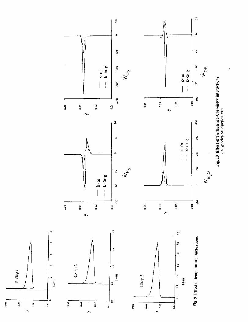
i

3_

_Q

3 3

>..,

o

° _

d

©

©

_J

L.

._=

L.

i N

_ .--i

r,i

E+

,:r

o--

i--i

-i

mm

o--r_J,u

33

3 3

I:

,I

.o

o

33

I

3 _

_Q

l. c_

©

_m

A

L

u_°_

_b

APPENDIX- D

Two-Equa!ionTurbu!enceModel forCompressible Reacting FlowsJ. R. Narayan

Reprinted from

AIAAJoumalVolume31, Number2, February1993,Pages398-401

IIA/AA_A publication of the

American Institute of Aeronautics and Astronautics, Inc.The AerospaceCenter, 370 L'Enfant Promenade,SWWashington, DC20024-2518

398 AIAA JOURNAL, VOL. 31, NO. 2: TECHNICAL NOTES

lieGE BI.ANK NOT FtLME_._

Two-Equation Turbulence Model for

Compressible Reacting Flows

J. R. Narayan*

NASA Ames Research Center,

Moffett Field, California 94035

Introduction

NE of the major areas of current interest where compu-tational fluid dynamics (CFD) is used extensively is the

development of advanced air-breathing propulsion systems forhypersonic vehicles. A hydrogen-fueled supersonic combus-

Received Jan. 13, 1992; revision received July 9, 1992; accepted forpublication July 10, 1992. Copyright © 1992 by the American Insti-tute of Aeronautics and Astronautics, Inc. All rights reserved.

*Research Scientist, MCAT Institute. Member AIAA.

400 AIAAJOURNAL, VOL. 31, NO. 2: TECHNICAL NOTES

comparison between the predictions and representative experi-mental data. 6,7 Here, C_ is defined as

d_ U_ + UEC,-

dx UI - U 2

and C_0 is its value for incompressible flow. KEPSI refers tothe predictions with compressibility correction included, and

KEPS2 refers to the predictions without the correction. RS

refers to the Reynolds stress closure predictions) The scatter

among the experimental data is indicative of the nature of

available data. The effect of compressibility on the mixing-

layer growth rate is to reduce the growth rate with increasingconvective Much number. The two-equation model without

the compressibility correction does not predict the reduced

growth rate with increasing compressibility. However, the

compressible two-equation model does predict this trend verywell. The close comparison between the Reynolds stress clo-

sure and the k-¢ model is important because for complicated

flowfields, such as that in the scramjet combustor, the higher-

order Reynolds stress closure may be very expensive to use.

The predictions agree well with experiment within the scatter in

the available data. It must be pointed out that there are other

compressibility correction models, similar to the one used

here, available today. However, a detailed comparison be-

tween such models is beyond the scope of this report.

Mixing between fuel and air and the ensuing chemical reac-tion is the main focus of study for a configuration such as the

scramjet combustor. The presence of turbulence and its effect

on the flowfield, especially the mixing aspect of it, is an impor-

tant part of such studies. A representative mixing dominated

reacting flow (hydrogen and air) is considered here. A seven-

step, seven-species HE-Air reaction model (Table 1) has beenused for the finite rate chemistry system considered here.

The test case studied is the reacting coaxial jet problem

(Figs. 3) for which the experimental data was obtained by

• , , G: , - G: -" ,0.0 0.5 1.0 0.0 0.5 0.0 0.5

/s,

0_' 0o.o s_, o15 o o.o 0.5 oo o15

V/D 1 •

0.0 ..t.H_° 0.5 0,0 0.5 0.0 0.5

0_ r I , , ,

o.o & 0.5 o.o o.5 o.o o15

a) Species mass fractions Hi, 02, HEO, and N2

1.50-- Pr*dictions

1.25 • Expermmtt

1.00 _..._ m,

/'8, 0.75

0,50

0.25

0.0010 20 30

z/D

b) Centeriine Hi distribution

Fig. 3 Reacting flow: co_Aal Jets.

Evans et al. s In the experiment, hydrogen at a temperature of251 K was injected (Much number = 2.0 and velocity = 2418

m/s) along the axis of a supersonic jet (Much number 1.9,

velocity= 1510 m/s) of vitiated air (temperature= 1495 K).

The species mass fractions in the alrstream are nitrogen =0.478, oxygen = 0.241, and water = 0.281. The fuel injector has

an inner diameter of 0.6525 cm and outer diameter of 0.9525

cm. The outer jet (air) diameter is 6.53 cm. The predicted

centerline distribution of hydrogen and the profiles of the

major species mass fractions (H 2, O2, HEO, NE) at three axiallocations are compared with experimental data in Figs. 3. In

these figures, D is the fuel injector outer diameter. The predic-

tions agree well with experiment in the region where the mixing

effects dominate. The discrepancy between the predictions and

experiment immediately downstream of the injector exit maybe due to the fact that the conditions set at the inlet location

(boundary condition for computations) in the calculations

may not match the exact experimental conditions. These con-ditions are unknown and, hence, could not be used for the

calculations. The predicted profiles of water vapor, which is anindication of the extent of reaction, agree reasonably well with

the experiment. The location of the peak in the profile isfarther into the airstream for the predictions than the experi-

ment indicates. This may be because the interaction betweenturbulence and chemistry is not fully accounted for in the

calculations. As mentioned earlier, the calculations account

for only the effect of temperature fluctuations on the reactionrate. In addition, correlations of order higher than 2 were

dropped from the model. Also, the experimental data itself

may not be very accurate. Given that, the compressible turbu-

lence model used here performs very well in predicting the

turbulent reacting flow.

Conclusions

A two-equation turbulence model (k-O has been modified to

be applicable for compressible flows by adapting a compress-

ibility correction model. Computation of compressible mixing

layers indicate that the decrease in the growth rate of the

mixing layer with increasing convective Mach number is well

predicted by the model. Comparisons of the predictions agree

very well with available experimental data and the predictionsof a compressible Reynolds stress closure. Preliminary studies

of reacting mixing problems involving dissimilar gases indicatethat the model is well suited for application to such flows. Thecomputations use a model for the effect of temperature fluctu-ations on the reaction rate in the finite rate chemistry model.

Further improvement to the model, especially the effect ofturbulent fluctuations in species concentrations on the produc-

tion rate, is necessary.

Acknowledgments

This work was supported by Theoretical Flow Physics

Branch, Fluid Mechanics Division, NASA Langley ResearchCenter under Contract NAS1-18599. The Technical Monitorwas J. P. Drummond.

References

ICarpenter, M. H., "Three-Dimensional Computations of Cross-Flow Injection and Combustion in a Supersonic Flow," AIAA Paper89-1870, June 1989.

2Narayan, J.R., "A Two-Equation Turbulence Model for Com-pressible Reacting Flows," AIAA Paper 91-0755, 29th Aerospace Sci-ences Meeting, Reno, NV, Jan. 1991.

3Narayan, J. R., and Sekar, B., "Computation of Turbulent HighSpeed Mixing Layers Using a Two-Equation Turbulence Model,"Proceedings of the CFD Symposium on Aeropropulsion, NASA LewisResearch Center, Cleveland, OH, April 1990.

4Sarkar, S., Erlebacher, G., Hussalni, M. Y., and Kreiss, H. O.,

"The Analysis and Modeling of Dilatational Terms in CompressibleTurbulence," NASA CR 181959, Dec. 1989.

5Jachimowski, C. J., "An Analytical Study of the Hydrogen-AirReaction Mechanism with Application to Scramjet Combustion,"NASA TP 2791, 1988.